1

Correlating Market Models Bruce Choy∗ , Tim Dun∗  and Erik Schlogl  

 

In  recent  years  the  LIBOR Market Model  (LMM)  (Brace, Gatarek & Musiela  (BGM)  1997, 

Jamshidian  1997,  Miltersen,  Sandmann  &  Sondermann  1997)  has  gained  acceptance  as  a 

practical and versatile model of  interest  rate dynamics. Based within a HJM  (Heath, Jarrow & 

Morton,  1992)  framework,  the model  concentrates  on  describing market  observable  forward 

LIBORs,  rather  than  the  mathematically  abstract  instantaneous  forward  rates,  and  has  the 

advantage of pricing interest rate caps and floors in a manner consistent with the popular Black 

(1976) formula. Though not strictly consistent from a theoretical viewpoint, pricing swaptions by 

application of  the Black  formula  is  also  standard practice  and has been  shown  to be  a highly 

accurate approximation within the LMM framework (see eg. Brace, Dun & Barton 2001). 

 

The key task for any practical implementation of an interest rate model is the calibration of the 

model to market prices, i.e. one requires that the LMM model parameters be consistent with 

liquid prices for at-the-money caps and swaptions. The main feature differentiating approaches 

to calibration of the LMM is how they treat correlation between forward LIBORs of different 

maturities.  

 

In theory, swaption prices carry information about correlation between forward LIBORs. 

However, calibration techniques in which correlation is an output typically struggle to 

simultaneously fit the caps and swaptions as well as produce reasonable yield curve correlations 

(eg BGM 1997, Gatarek 2000, Hull 2000, Dun 2000 and the methods described in the book by 

Brigo and Mercurio 2001). On the other hand, approaches which take the correlations explicitly 

as an input to the calibration (eg. Pedersen 1998, Wu 2002) report very encouraging results. 

Brace & Womersley (2000) use a semidefinite programming technique to simultaneously 

calibrate volatilities and correlations to swaption and caplet prices. However, they recognise that 

the problem is highly underdetermined and resolve this by optimising to select the closest 

possible fit to historically estimated correlations. Rebonato (1999) attributes this indeterminacy 

to the fact that volatilities can depend on both calendar and maturity time. Unfortunately, this 

                                                  ∗  ANZ  Investment Bank. Bruce Choy has since moved  to Commonwealth Bank of Australia. The views presented here are do not necessarily reflect the views of either organisation. ∗  ANZ  Investment Bank. Bruce Choy has since moved  to Commonwealth Bank of Australia. The views presented here are do not necessarily reflect the views of either organisation.  School of Finance and Economics, University of Technology, Sydney. 

  2

cannot be resolved by making volatilities depend solely on time to maturity, since under this 

assumption one cannot even fit observed prices for at-the-money caps on days when the implied 

volatilities are sloping steeply downward with respect to cap length.  

 

Given the current state of the literature, the question of which is the most appropriate way to 

calibrate the LMM thus hinges on how the calibration method should deal with correlation. The 

aim of the present paper is to answer this question by exploring two points:  

 

1.  Is there sufficient information contained in swaption prices to calibrate correlation? 

2.  What are the consequences of the calibration problem being highly underdetermined? 

In particular, does it mean that the prices calculated using a calibrated LMM, e.g. for 

Bermudan swaptions or for spread options, are arbitrary and unreliable? 

 

To this end, we conduct a series of experiments using the Pedersen (1998) calibration approach. 

After briefly summarising this method, we review the different concepts of correlation relevant 

to the LMM. The potential inconsistency between historical and implied correlation is found not 

to be an issue. We analyse the sensitivity of swaption prices and the calibrated volatility levels to 

correlations, and also study the trade-off between fitting correlations and fitting a calendar-time 

dependence of volatility. Subsequently, we discuss the effects of calibration ambiguity on 

derivatives priced off the calibrated model. 

 

Pedersen Calibration 

 

In the LMM, volatility and correlation are described via the vector volatility function  ( )Tt,γ , 

dependent on calendar time  t  and maturity time T . The Pedersen calibration method employs a 

completely non-parametric description of this volatility, where the ith factor is given by 

( ) ( ) kjiii xtTt ,,',', γγγ ==  for  [ )jj ttt ,1−∈ ,  [ )kk xxx ,1−∈  

where  tTx −=  is forward time and  jt ,  calnj ,...,1= , and  kx ,  fornk ,...,1=  define respectively 

the calendar and forward time intervals for which the piece-wise constant volatility applies. For a 

model containing  facn  factors, this approach requires  forcalfac nnn ..  parameters to fully define the 

volatility, a number which can soon become computationally cumbersome for reasonable choices 

of the number of factors and the granularity of calendar and forward time.  

 

  3

Pedersen reduces the number of parameters by specifying the volatility in terms of a  forcal nn ×  

matrix (termed the volatility grid) and a  forfor nn ×  matrix of yield curve correlations. Thus the 

volatility grid allows for the specification of both calendar and forward time dependence, while 

correlation is assumed to be constant. The correlations are exogenous inputs, typically 

determined via analysis of historical data, and the Pedersen volatility  kji ,,'γ  is derived from the 

volatility grid and the correlation matrix via principal components analysis (PCA). This approach 

has the advantage that multi-factor calibrations are straightforward to determine, with the 

number of factors in the volatility function simply equal to the number of dominant eigenvectors 

extracted from the PCA. 

 

The Pedersen calibration applies a numerical optimisation technique to the volatility grid until a 

sufficiently close fit is obtained between the market-observed and model-implied prices of 

vanilla interest rate caps and swaptions. Additional smoothness constraints are applied to the grid 

(in both the calendar and forward time dimensions) in order to further reduce the degrees of 

freedom in the optimisation, as well as promote a more reasonable form of the solution. With 

such a large number of parameters available, smoothing also reduces the likelihood of the 

calibration over-fitting the input data. 

 

Yield Curve Correlation 

 

In practice, yield curve correlation is described in terms of correlations between forward 

LIBORs, where it is assumed that these rates follow a joint lognormal distribution (that is, the 

natural logarithm of the forward rates is jointly normally distributed). Assuming both this and 

that the distribution is constant in time allows the yield curve correlations to be determined from 

a time series of historical yield curve data. The result of such an analysis on AUD data is shown 

in Figure 1. 

Correlations in the LMM can be approximated from the volatility function via an analysis of the 

quadratic covariation of the forward LIBORs. For a series of consecutive LIBORs running 

between equi-spaced maturity points  iT , such an analysis reveals that at any one instant  t , the jth 

and kth LIBORs are correlated as 

( ) ( )( ) ( )kj

kjkj TtTt

TtTt,,

,,, γγ

γγρ

⋅= . 

  4

This is termed instantaneous correlation and needs to be integrated over time before we can 

obtain something that has any intuitive meaning or practical use. The integration can be 

performed in two ways; the first keeps the LIBOR maturity points constant, leading to the 

expression 

( ) ( )

( ) ( ) dsTsdsTs

dsTsTs

T

k

T

j

T

kjkj 2

00

2

0,

,,

,,

∫∫

∫ ⋅=

γγ

γγρ . (1) 

 

This is called terminal correlation and while it is important in the pricing of derivatives such as 

European spread options, it cannot be determined easily from historical correlation. Terms of this 

type also enter into the calculation of swaption prices, thus theoretically market prices for 

swaptions carry information about terminal correlation. If one were to speak of implied 

correlation, this would be the appropriate correlation concept. 

 

The second way to integrate instantaneous correlation moves the LIBOR maturity points along 

with calendar time 

( ) ( )

( ) ( ) dssTsdssTs

dssTssTs

T

k

T

j

T

kjkj 2

00

2

0,

,,

,,

∫∫

∫++

+⋅+=

γγ

γγρ   (2) 

 

and thus represents correlations between LIBORs with a fixed time to maturity. This is 

analogous to what is happening when we calculate historical correlations from past yield curve 

data, and for this reason we term this pseudo-historical correlation. 

 

Equations (1) and (2) are only approximations to the correlation as they assume the contribution 

of the level dependent drift term in the stochastic differential equation (SDE) for the LIBORs to 

be negligible. 

 

Correlation in the Pedersen Calibration 

 

Calibration involves fitting market prices, implying that we require terminal correlations. Using 

a calibration method which takes correlation estimated from historical data as an input thus raises 

the question whether the distinction between (1) and (2) has any significant impact on 

correlations in a calibrated model. One would say that this is not the case if the pseudo-historical 

  5

correlations generated by a calibrated model closely match the (historical) correlations, which 

were input into the calibration. In passing, this would also resolve the issue whether the 

contribution of the level dependent drift term is indeed negligible for purposes of calibration. 

 

Consider Figure 2, which displays pseudo-historical correlations resulting from calibration to 

AUD cap and swaption data from the 4th January 2002. The historical correlations of Figure 1 

were employed as inputs to the calibration, and 1, 3 and 8 factor volatility functions produced. 

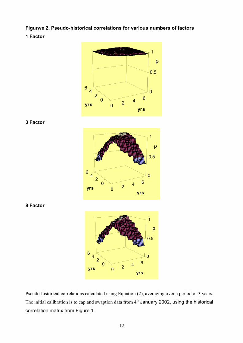
Equation (2) was used to calculate the correlations. As could be expected, a single factor model 

implies almost perfect correlation between all parts of the yield curve, while 3 and 8 factor 

models are not only successful in producing correlation of a plausible shape, but also closely 

match the shape and magnitude of the input historical correlations. This thus gives us the 

comforting result that historical correlations fed into the Pedersen calibration method can be 

successfully recovered as output from the other end of the model. This is not a trivial 

observation, since the estimation of historical correlations assumes time homogeneity (i.e. 

dependence of volatilities only on time to maturity, not calendar time), while calibrated 

volatilities typically violate this assumption. 

 

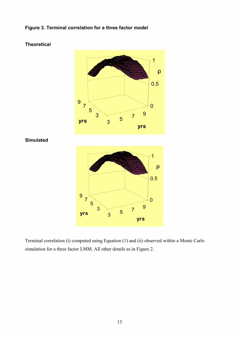
To analyse the terminal correlations as defined by Equation (1), consider Figure 3. The 

correlations for a point 3 years in the future are displayed, calculated analytically for a calibrated 

3 factor model. The results are compared against the correlations observed within a Monte Carlo 

simulation of the model with the same volatility function, and can be seen to agree favourably, 

providing further evidence that the influence of the level dependent drift can be ignored. We also 

see that compared to the historical correlation, terminal correlations show greater 

interdependence, with all the values shifted closer towards perfect correlation.  

 

While not shown in this article, all these results can also be extended to swap rate correlations, 

with terminal correlations showing values closer to unity, and model predicted pseudo-historical 

correlations matching those contained in the historical yield curve data. This is noteworthy in 

that historical swap rate correlations are matched even though it is the LIBOR correlations that 

are fed into the model. While these results were produced on AUD data, they are equally 

applicable to USD data. 

 

 

 

  6

Swaption Sensitivity 

 

It is commonly known that swaptions are dependent on correlations within the yield curve, but 

there is little in the academic literature about how strong this dependence really is. To test this, 

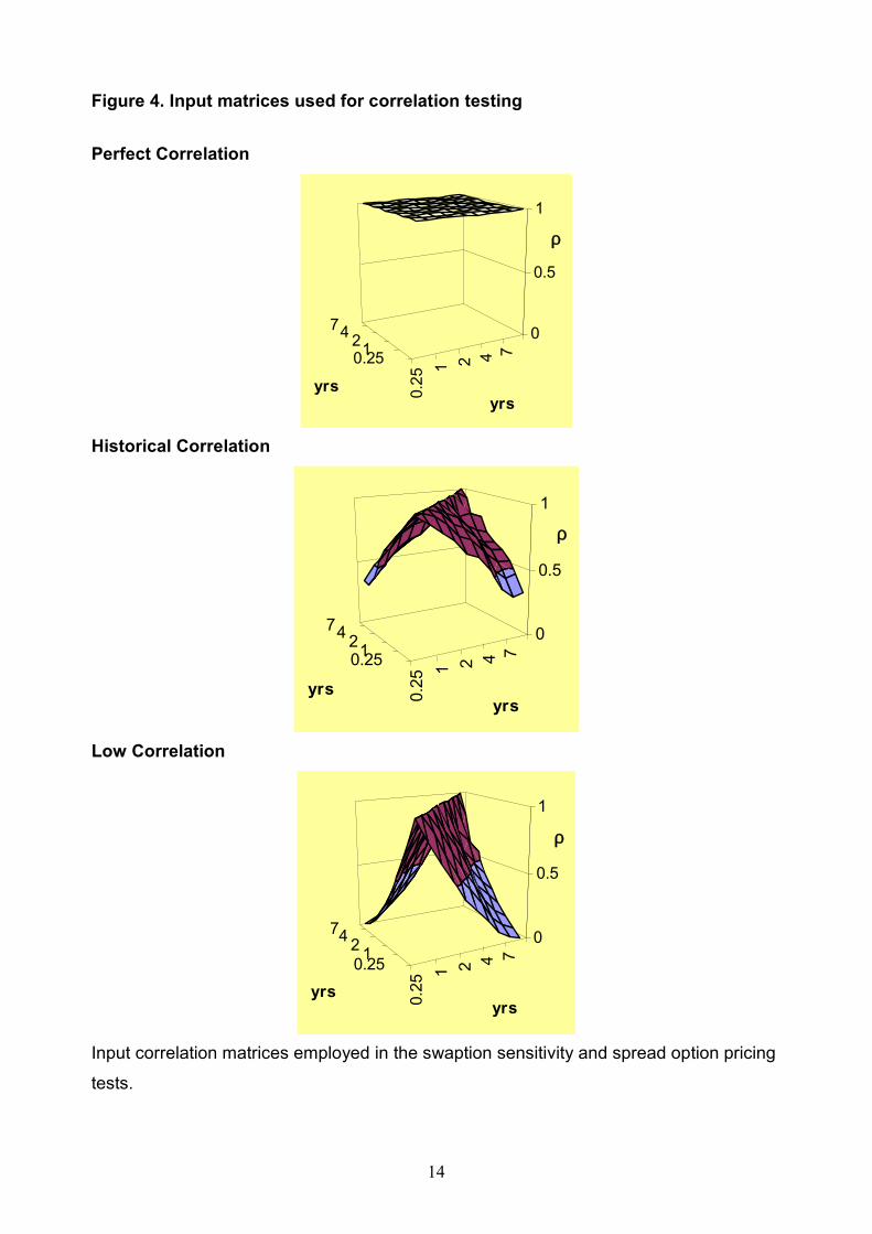
we have chosen three significantly different matrices representing a spectrum of possible yield 

curve correlations, as shown in Figure 4. The matrices include one implying perfect correlation, 

the historical matrix used previously, and an altered version of the historical matrix implying low 

correlations between rates. 

 

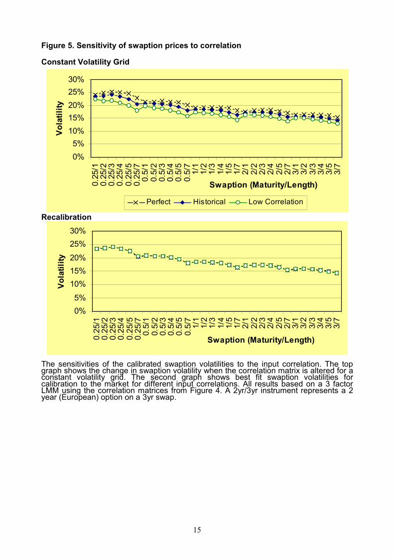
The effect of these correlation matrices on swaption prices is displayed in the upper graph in 

Figure 5 where, in each case, the correlation is altered while holding the Pedersen volatility grid 

constant. For clarity, we represent swaption prices in terms of their Black implied volatilities. 

From the graph is it evident that even large changes in correlation lead to only minor adjustments 

in the swaption volatility, suggesting that correlation has only a second order effect on swaption 

prices. If anything, these results are an exaggeration of the true effect, as we have not corrected 

for the effect of the scaling of the Pedersen volatility function that occurs during the PCA. As a 

consequence of this, it is evident that swaptions do not contain much correlation information. 

This has previously been observed by Brigo/Mercurio (2001). However, in the calibration 

method applied here, we do not see the difficulties they encountered when fixing correlations 

and adjusting volatility levels to calibrate cap and swaption prices. Here, the fit to market prices 

is good (see Table A) and the correlation structure (Figures 2 and 3) and volatility grid (Figure 6) 

appear reasonable. We achieve results of similar quality when running the Pedersen calibration 

on the data from Chapter 7 of Brigo & Mercurio, as well as for the case of steeply downward 

sloping volatility considered problematic in Brace & Womersley (2000). 

 

The second graph in Figure 5 shows the effect of using identical vanilla instruments yet different 

correlation matrices as inputs to the calibration routine. In each case the swaptions are calibrated 

equally well, demonstrating that the Pedersen routine is flexible enough to fit all the swaptions 

regardless of the correlation specified. While this indicates the significant power of the routine, it 

also means that it is extremely important to get the input correlation right in the first place, as the 

calibration wonít tell us if our correlation is unreasonable.  

 

 

 

  7

Correlation vs Calendar Time Dependence 

 

In addition to the observation that swaption prices are not very sensitive to correlation, the trade-

off between fitting correlations and fitting a calendar-time dependence of volatility, to which 

Rebonato alludes in his 1999 book, is another potential explanation of why one can reconcile 

nearly any arbitrary correlation structure with market prices for caps and swaptions. Taking this 

a step further, one might suggest that there is a choice to either hold the correlation fixed and 

achieve the fit by adjusting the calendar-time dependence of volatility, or vice versa. This would 

mean that not only is there some uncertainty about the correct price of correlation-dependent 

exotics relative to the market prices of vanilla products, but also about the correct price of 

instruments which are sensitive to how total volatility to a given time horizon is distributed over 

calendar time. The latter consequence is potentially far more important, since it affects 

Bermudan swaptions. 

 

However, it turns out that even radically varying the input correlation matrix does not result in a 

substantial change in the calendar-time dependence of the calibrated volatilities, as can be seen 

in Figure 6. Unsurprisingly, this also means that Bermudan swaption prices are not much 

affected, see Figure 7. It would appear that the calendar-time dependence of the calibrated 

volatilities is more driven by the volatility levels implicit in observed prices, rather than the need 

to reconcile these prices with a given correlation structure. This is quite natural considering that 

on some days cap prices alone (which do not depend on correlation) force a calendar-time 

dependence of volatility in order to achieve a fit. 

 

This also goes to explain why practical experience with calibration on market data rarely is in 

line with the intuitive result that more factors (i.e. permitting a higher rank for the forward 

LIBOR covariance matrix) reduces the calendar-time dependence of calibrated volatilities. This 

expected effect can be demonstrated on simulated data (i.e. volatilities will be time-dependent in 

a two-factor model calibrated to prices generated from a four-factor model without time-

dependence), however, real data appear to have a certain level of intrinsic calendar-time 

dependence of volatility levels. Another version of the calibration procedure, where time 

dependence (or the lack thereof) is an input and the correlation structure is determined by the 

calibration, would therefore be quite unstable. 

 

 

  8

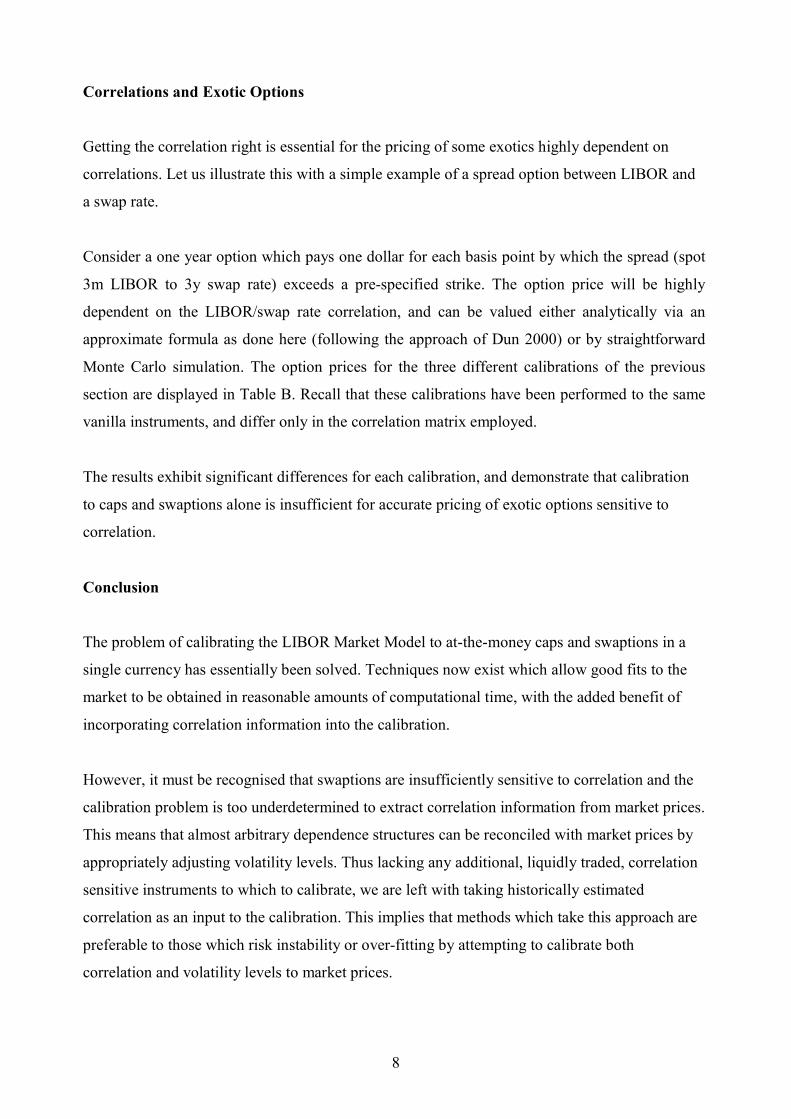
Correlations and Exotic Options 

 

Getting the correlation right is essential for the pricing of some exotics highly dependent on 

correlations. Let us illustrate this with a simple example of a spread option between LIBOR and 

a swap rate.  

 

Consider a one year option which pays one dollar for each basis point by which the spread (spot 

3m  LIBOR  to  3y  swap  rate)  exceeds  a  pre-specified  strike.  The  option  price will  be  highly 

dependent  on  the  LIBOR/swap  rate  correlation,  and  can  be  valued  either  analytically  via  an 

approximate formula as done here (following  the approach of Dun 2000) or by straightforward 

Monte Carlo  simulation. The  option  prices  for  the  three  different  calibrations  of  the  previous 

section are displayed in Table B. Recall that these calibrations have been performed to the same 

vanilla instruments, and differ only in the correlation matrix employed. 

 

The results exhibit significant differences for each calibration, and demonstrate that calibration 

to caps and swaptions alone is insufficient for accurate pricing of exotic options sensitive to 

correlation. 

 

Conclusion 

 

The problem of calibrating the LIBOR Market Model to at-the-money caps and swaptions in a 

single currency has essentially been solved. Techniques now exist which allow good fits to the 

market to be obtained in reasonable amounts of computational time, with the added benefit of 

incorporating correlation information into the calibration. 

 

However, it must be recognised that swaptions are insufficiently sensitive to correlation and the 

calibration problem is too underdetermined to extract correlation information from market prices. 

This means that almost arbitrary dependence structures can be reconciled with market prices by 

appropriately adjusting volatility levels. Thus lacking any additional, liquidly traded, correlation 

sensitive instruments to which to calibrate, we are left with taking historically estimated 

correlation as an input to the calibration. This implies that methods which take this approach are 

preferable to those which risk instability or over-fitting by attempting to calibrate both 

correlation and volatility levels to market prices. 

 

  9

Specifically, the Pedersen (1998) calibration method studied here shows remarkable robustness, 

achieving satisfactory results against Brigo & Mercurioís criteria (cf.  their Chapter 7.5): Small 

calibration  error,  regular  correlation  structures  and  a  relatively  smooth  evolution  of  the  term 

structure  of  volatilities  over  time.  In  addition,  it  is  encouraging  that  historically  estimated 

correlations fed  into  the model are faithfully reproduced  in  the model output. The fact  that  the 

calendar  time dependence  is not quite  as  stable  as one might wish  from a  theoretical point of 

view appears to be a feature of the data and the LMM itself, rather than the calibration method, 

since  the  input correlation structure and  the number of factors has  little  impact on  the calendar 

time dependence of calibrated volatilities. This is perhaps most akin to the calibration of the drift 

in an interest rate term structure model of the Hull/White (1990) type to observed bond prices ñ 

there,  too,  the  time  dependence  is  simply  driven  by  the  data without  any  further  qualitative 

justification. 

 

The fact that we cannot reliably extract the ì marketís viewî  of correlation from liquidly traded 

instruments means that pricing exotic derivatives off a calibrated LMM is subject to an important 

caveat: For exotics very sensitive to correlation, such as spread options, one is effectively 

calculating the price on the basis of a historical estimate. This should be treated with the same 

amount of caution as one would a Black/Scholes price calculated using historical volatility. 

Fortunately, by transaction volume, the most important type of non-standard interest rate 

derivative is not affected by this: Bermudan swaption prices do not react significantly when the 

LMM is calibrated to a different correlation structure. 

 

References 

 

Brace A, T Dun and G Barton, 2001, Towards a Central Interest Rate Model.In: Jouini, E, J 

Cvitanic and M Musiela (eds.) Option Pricing, Interest Rates and Risk Management, 

Cambridge University Press. 

Brace A, D Gatarek and M Musiela, 1997, The market model of interest rate dynamics. 

Mathematical Finance 7, pages 127-154. 

Brace A and R Womersley, 2000, Exact fit to the swaption volatility matrix using semi-definite 

programming. Working paper, National Australia Bank and University of New South 

Wales 

Brigo D and F Mercurio, 2001, Interest Rate Models: Theory and Practice. Springer-Verlag. 

  10

Dun T, 2000, Numerical studies on the lognormal forward interest rate model. Ph.D thesis, 

University of Sydney. 

Gatarek D, 2000, Modelling without tears. Risk September 2002, pages S20-S24. 

Heath D, R Jarrow and A Morton, 1992, Bond pricing and the term structure of interest rates: A 

new methodology for contingent claim valuation. Econometrica 60 (1), pages 77-105. 

Hull J, 2000, The essentials of the LMM. Risk December 2002, pages 126-129. 

Hull J and A White 1990, Pricing Interest Rate Derivative Securities. Review of Financial 

Studies, pages 573-592. 

Jamshidian F, 1997, Libor and swap market models and measures. Finance and Stochastics 1 

(4), pages 293-330. 

Miltersen K, K Sandmann and D Sondermann, 1997, Closed form solutions for term structure 

derivatives with lognormal interest rates. Journal of Finance 52, pages 409-430. 

Pedersen M, 1998, Calibrating Libor market models. Working paper, Financial Research 

Department, Simcorp A/S. 

Rebonato R, 1999, Volatility and correlation in the pricing of equity, FX and Interest-rate 

options. John Wiley & Sons. 

Wu L, 2002, Fast at-the-money calibration of the LIBOR market model through Lagrange 

multipliers. Journal of Computational Finance 6 Winter (2002/3), pages 39-77. 

 

 

  11

 

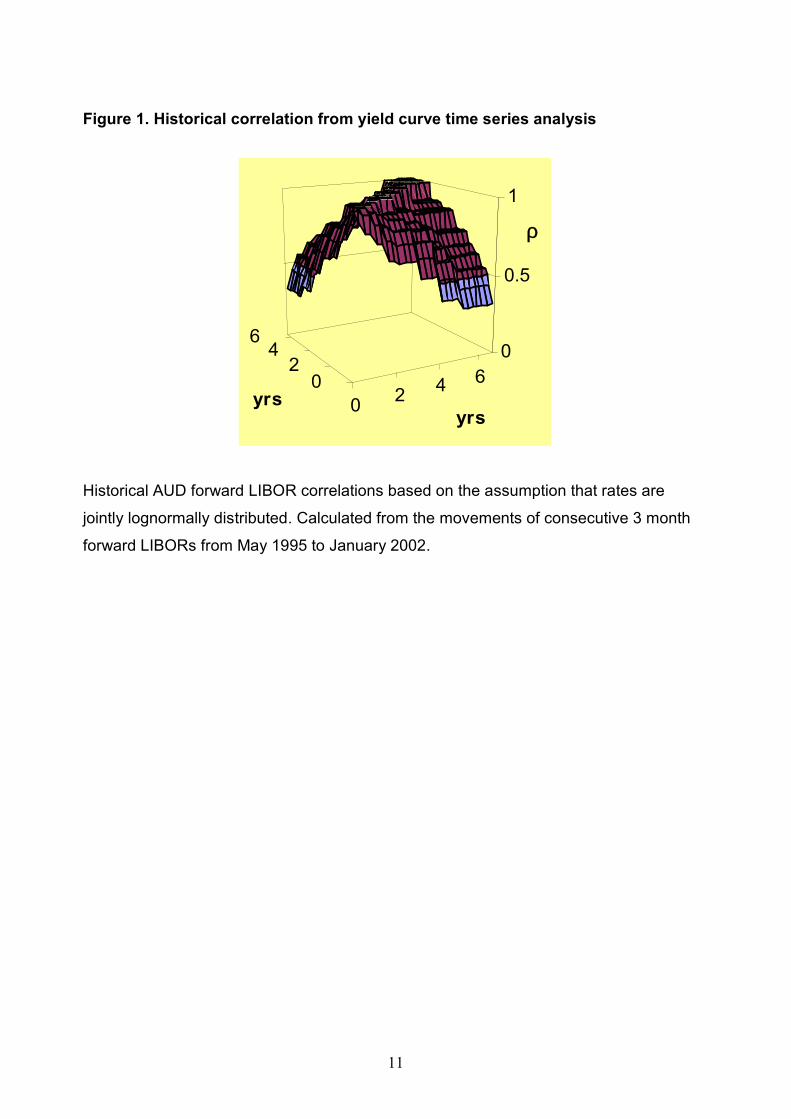
Figure 1. Historical correlation from yield curve time series analysis  

0 2 4 602

46

0

0.5

1

ρ

yrsyrs

 

 

Historical AUD forward LIBOR correlations based on the assumption that rates are 

jointly lognormally distributed. Calculated from the movements of consecutive 3 month 

forward LIBORs from May 1995 to January 2002.  

  

  12

Figurwe 2. Pseudo-historical correlations for various numbers of factors 1 Factor 

0 2 4 602

46

0

0.5

1

ρ

yrsyrs

 3 Factor 

0 2 4 602

46

0

0.5

1

ρ

yrsyrs

 8 Factor 

0 2 4 602

46

0

0.5

1

ρ

yrsyrs

  

Pseudo-historical correlations calculated using Equation (2), averaging over a period of 3 years. 

The initial calibration is to cap and swaption data from 4th January 2002, using the historical 

correlation matrix from Figure 1.

  13

Figure 3. Terminal correlation for a three factor model  

Theoretical 

3 5 7 935

79

0

0.5

1

ρ

yrsyrs

 Simulated 

3 5 7 935

79

0

0.5

1

ρ

yrsyrs

  

Terminal correlation (i) computed using Equation (1) and (ii) observed within a Monte Carlo 

simulation for a three factor LMM. All other details as in Figure 2. 

 

  14

Figure 4. Input matrices used for correlation testing  

Perfect Correlation 

0.251 2 4 70.251

247 0

0.5

1

ρ

yrsyrs

 

Historical Correlation 0.251 2 4 70.251

247 0

0.5

1

ρ

yrsyrs

 

Low Correlation 

0.251 2 4 70.251

247 0

0.5

1

ρ

yrsyrs

 

Input correlation matrices employed in the swaption sensitivity and spread option pricing 

tests.  

  15

Figure 5. Sensitivity of swaption prices to correlation  Constant Volatility Grid 

0%5%10%15%20%25%30%

0.25/1

0.25/2

0.25/3

0.25/4

0.25/5

0.25/7

0.5/1

0.5/2

0.5/3

0.5/4

0.5/5

0.5/7

1/1

1/2

1/3

1/4

1/5

1/7

2/1

2/2

2/3

2/4

2/5

2/7

3/1

3/2

3/3

3/4

3/5

3/7

Swaption (Maturity/Length) 

Volatility

Perfect Historical Low Correlation  Recalibration 

0%5%10%15%20%25%30%

0.25/1

0.25/2

0.25/3

0.25/4

0.25/5

0.25/7

0.5/1

0.5/2

0.5/3

0.5/4

0.5/5

0.5/7

1/1

1/2

1/3

1/4

1/5

1/7

2/1

2/2

2/3

2/4

2/5

2/7

3/1

3/2

3/3

3/4

3/5

3/7

Swaption (Maturity/Length) 

Volatility

   The  sensitivities of  the  calibrated  swaption  volatilities  to  the  input  correlation. The  top graph shows the change in swaption volatility when the correlation matrix is altered for a constant  volatility  grid.  The  second  graph  shows  best  fit  swaption  volatilities  for calibration  to  the market  for different  input correlations. All  results based on a 3  factor LMM using  the correlation matrices  from Figure 4. A 2yr/3yr  instrument represents a 2 year (European) option on a 3yr swap.  

 

  16

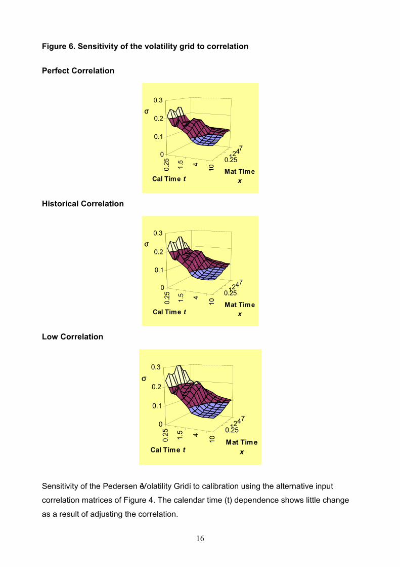
Figure 6. Sensitivity of the volatility grid to correlation  

Perfect Correlation 

0.251247

0.25 1.5 4

10

0

0.1

0.2

0.3σ

Mat TimexCal Time  t

 

Historical Correlation 

0.251247

0.25 1.5 4

10

0

0.1

0.2

0.3σ

Mat TimexCal Time  t

 

Low Correlation 

0.251247

0.25 1.5 4

10

0

0.1

0.2

0.3σ

Mat TimexCal Time t

  

Sensitivity of the Pedersen ëVolatility Gridí to calibration using the alternative input 

correlation matrices of Figure 4. The calendar time (t) dependence shows little change 

as a result of adjusting the correlation. 

  17

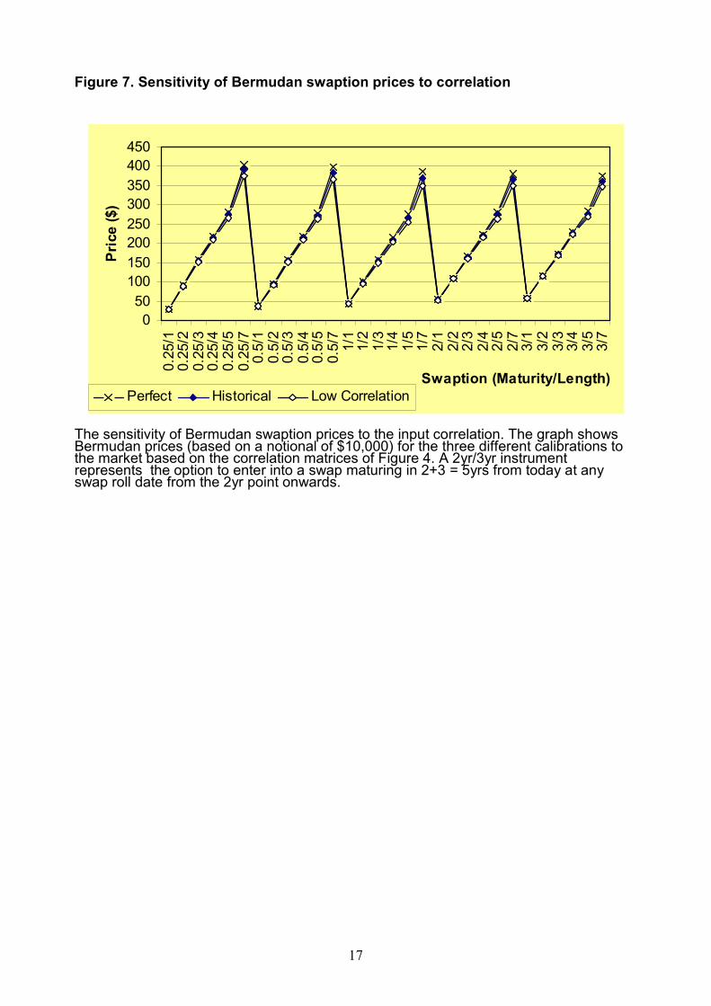
Figure 7. Sensitivity of Bermudan swaption prices to correlation   

050100150200250300350400450

0.25/1

0.25/2

0.25/3

0.25/4

0.25/5

0.25/7

0.5/1

0.5/2

0.5/3

0.5/4

0.5/5

0.5/7

1/1

1/2

1/3

1/4

1/5

1/7

2/1

2/2

2/3

2/4

2/5

2/7

3/1

3/2

3/3

3/4

3/5

3/7

Swaption (Maturity/Length)

Price ($)

Perfect Historical Low Correlation  

The sensitivity of Bermudan swaption prices to the input correlation. The graph shows Bermudan prices (based on a notional of $10,000) for the three different calibrations to the market based on the correlation matrices of Figure 4. A 2yr/3yr instrument represents  the option to enter into a swap maturing in 2+3 = 5yrs from today at any swap roll date from the 2yr point onwards.  

 

  18

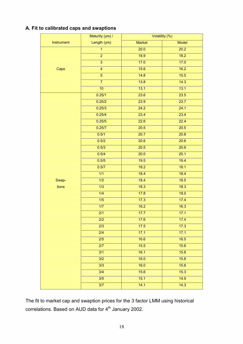
A. Fit to calibrated caps and swaptions Volatility (%)  

Instrument 

Maturity (yrs) / 

Length (yrs)  Market  Model 

  1  20.0  20.2 

  2  18.9  18.2 

  3  17.0  17.0 

Caps  4  15.6  16.2 

  5  14.8  15.5 

  7  13.8  14.3 

  10  13.1  13.1 

  0.25/1  23.6  23.5 

  0.25/2  23.9  23.7 

  0.25/3  24.2  24.1 

  0.25/4  23.4  23.4 

  0.25/5  22.6  22.4 

  0.25/7  20.5  20.5 

  0.5/1  20.7  20.8 

  0.5/2  20.6  20.6 

  0.5/3  20.5  20.6 

  0.5/4  20.0  20.1 

  0.5/5  19.5  19.4 

  0.5/7  18.2  18.1 

  1/1  18.4  18.4 

Swap-  1/2  18.4  18.5 

tions  1/3  18.3  18.3 

  1/4  17.8  18.0 

  1/5  17.3  17.4 

  1/7  16.2  16.3 

  2/1  17.7  17.1 

  2/2  17.6  17.4 

  2/3  17.5  17.3 

  2/4  17.1  17.1 

  2/5  16.6  16.5 

  2/7  15.5  15.6 

  3/1  16.1  15.8 

  3/2  16.0  15.8 

  3/3  16.0  15.6 

  3/4  15.6  15.3 

  3/5  15.1  14.9 

  3/7  14.1  14.3 

 

The fit to market cap and swaption prices for the 3 factor LMM using historical 

correlations. Based on AUD data for 4th January 2002. 

  19

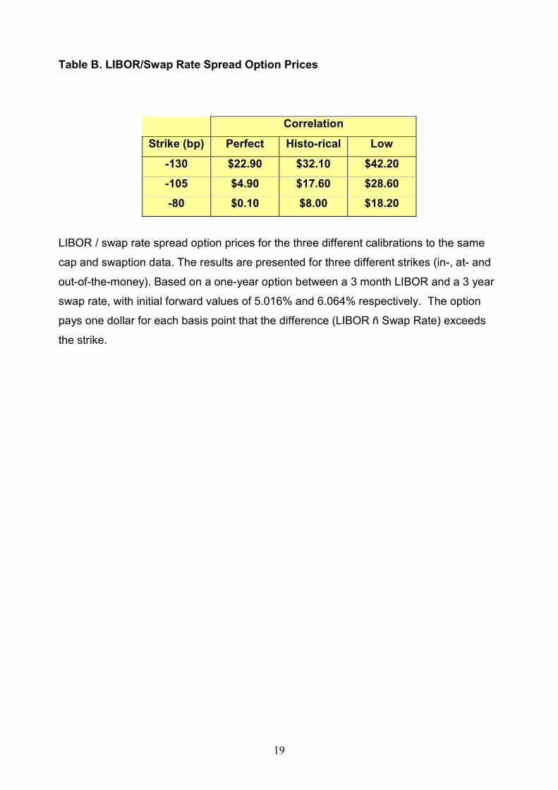
Table B. LIBOR/Swap Rate Spread Option Prices  

 

  Correlation 

Strike (bp)  Perfect  Histo-rical  Low 

-130  $22.90  $32.10  $42.20 -105  $4.90  $17.60  $28.60 -80  $0.10  $8.00  $18.20 

 

LIBOR / swap rate spread option prices for the three different calibrations to the same 

cap and swaption data. The results are presented for three different strikes (in-, at- and 

out-of-the-money). Based on a one-year option between a 3 month LIBOR and a 3 year 

swap rate, with initial forward values of 5.016% and 6.064% respectively.  The option 

pays one dollar for each basis point that the difference (LIBOR ñ Swap Rate) exceeds 

the strike.