Corporate Investment and Asset Price Dynamics ...faculty.haas.berkeley.edu/garleanu/ReadingGroup_AP_Sp2012/Carlson... · Corporate Investment and Asset Price Dynamics: ... Robert

THE JOURNAL OF FINANCE • VOL. LIX, NO. 6 • DECEMBER 2004

Corporate Investment and Asset Price Dynamics:Implications for the Cross-section of Returns

MURRAY CARLSON, ADLAI FISHER, and RON GIAMMARINO∗

ABSTRACT

We show that corporate investment decisions can explain the conditional dynamicsin expected asset returns. Our approach is similar in spirit to Berk, Green, and Naik(1999), but we introduce to the investment problem operating leverage, reversible realoptions, fixed adjustment costs, and finite growth opportunities. Asset betas vary overtime with historical investment decisions and the current product market demand.Book-to-market effects emerge and relate to operating leverage, while size capturesthe residual importance of growth options relative to assets in place. We estimateand test the model using simulation methods and reproduce portfolio excess returnscomparable to the data.

CORPORATE INVESTMENT DECISIONS are often evaluated in a real options context,1

and option exercise can change the riskiness of a firm in various ways. Forexample, if growth opportunities are finite, the decision to invest changes theratio of growth options to assets in place. Additionally, the resulting increasein physical capital may generate operating leverage through long-term obliga-tions, including the fixed operating costs of a larger plant, wage contracts, andcommitments to suppliers. It is natural to conclude that expected returns mightbe related to current and historical investment decisions of the firm.

The empirical literature has long recognized a need to account for thedynamic structure of risk when testing asset pricing models.2 A small butgrowing literature that endogenizes expected returns through firm-level

∗Sauder School of Business, University of British Columbia. We appreciate helpful commentsfrom Jonathan Berk, Peter Christoffersen, Lorenzo Garlappi, the editor Rick Green, the refereeJoao Gomes, Rob Heinkel, Burton Hollifield, Leonid Kogan, Ali Lazrak, Eduardo Schwartz, RamanUppal, Tan Wang, Yong Wang, Robert Whitelaw, and seminar participants at the University ofAlberta, UBC, the 2003 conference on Simulation Based and Finite Sample Inference in Financeat Laval University, the 2003 Phillips Hager and North Summer Finance Conference at UBC,the 2003 Northern Finance Association meetings, and the 2004 American Finance AssociationMeetings in San Diego. Support for this project from the Bureau of Asset Management at UBC andthe Social Sciences and Humanities Research Council of Canada (grant number 410-2003-0741) isgratefully acknowledged.

1 This approach was pioneered by McDonald and Siegel (1985, 1986) and Brennan and Schwartz(1985), and has been extended in many directions. See Dixit and Pindyck (1994) for a detailedanalysis of the literature.

2 Hansen and Richard (1987) make this point theoretically. To address the issue, typical ap-plications use empirically or theoretically motivated instruments as conditioning variables. Twoexamples are Jagannathan and Wang (1996) and Ferson and Harvey (1999).

2577

2578 The Journal of Finance

decisions has begun to provide theoretical structure for risk and return dy-namics. Motivated by asset price anomalies,3 Berk, Green, and Naik (1999,hereafter BGN) were among the first to establish a link between investmentdecisions, the riskiness of assets-in-place, and expected returns.4 Their modelassumes that investment opportunities are heterogeneous in risk. This wouldtypically make a complete description of firm assets cumbersome, but theirmodel simplifies so that size and book-to-market are sufficient statistics forthe aggregate risk of assets in place.

We contribute to this line of research by developing two dynamic models.These differ in their technical details, but rely on the same economic forcesto relate endogenous firm investment to expected return. We arrive at a neweconomic role for operating leverage in explaining the book-to-market effect.When demand for a firm’s product decreases, equity value falls relative to thecapital stock, proxied by book value. Assuming that fixed operating costs areproportional to capital, the riskiness of returns increases due to greater oper-ating leverage. We also incorporate limits to growth in both our models, andshow that this is important for obtaining an independent size effect. Our firstmodel permits closed-form solutions in a stylized setting, allowing us to ex-amine the relationship between size and book-to-market for a single firm. Thesecond uses more realistic assumptions and gives stationary dynamics for across-section of firms. This permits structural estimation using the simulatedmethod of moments.

In the first model, a single all-equity firm faces stochastic iso-elastic demandin its output market. The unique exogenous state variable is the demand level,driven by a lognormal diffusion. The firm may expand the capacity a finitenumber of times, and a fixed adjustment cost is incurred each time operationsare expanded. Operating leverage results from per-period fixed operating coststhat increase in the capital level. The underlying revenue betas are assumed tobe constant, but firm betas are nonetheless time-varying and reflect historicalinvestment as well as current demand.

Our second model is based on more general assumptions, chosen to yield astructural empirical model of a cross-section of firms in a stationary, dynamicenvironment. We again model monopolistic firms, but stochastic demand nowhas both systematic and idiosyncratic components. We prohibit demand fromreaching arbitrarily high levels by using reflecting barriers. This assumptionreflects the economic intuition that growth becomes more difficult as firms be-come larger.5 During each period, firms: (1) set output at monopoly levels, withthe restriction that output not exceed capacity; (2) generate revenues and payfixed operating costs that are proportional to the amount of capital currentlyemployed; (3) make a decision to expand or reduce capacity, and in so doing,

3 Fama and French (1992) provide summary evidence on the ability of size and book-to-marketto explain returns. There is some debate as to whether this is due to factor risks (Fama and French(1993)) or priced characteristics (Daniel and Titman (1997)).

4 Further work in this area includes Gomes, Kogan, and Zhang (2003), Zhang (2003), and Cooper(2003).

5 Evans (1987) and Hall (1987) give evidence that firm growth rates decline with size.

Corporate Investment and Asset Price Dynamics 2579

pay a two-part adjustment cost, one part fixed and the other proportional to thechange in capital, or (4) exercise, at no cost, a one-time abandonment option todiscontinue all future operations. The economy is made stationary by allowingentry of new firms when existing firms exit. In this setting, adjustment costsgive rise to lumpy investment and firms build plants that may be larger orsmaller than they currently need in order to reduce adjustment costs. Fixedoperating costs reduce incentives to invest and motivate downsizing when de-mand falls. Firm risk is again related to firm size and book-to-market ratios,and these effects appear unconditionally in portfolios that are formed using thestandard sorting procedures.

We use numerical solution techniques to solve the model and simulatedmethod of moments for estimation. This approach provides statistical measuresof the significance of estimated parameters. The structural model generatesindependent size and book-to-market effects for portfolios, with magnitudesequivalent to those in actual monthly returns from the past 40 years. Parame-ter estimates from the model indicate statistically significant fixed costs, capitalacquisition costs, and demand volatility in explaining actual returns. This pro-vides a quantitative measure of the importance of operating leverage and realoptions within the model.

Our theoretical model of the firm adds to the existing literature by expandingthe description of the firm’s operating environment in an important way. Ourspecification gives rise to book-to-market and size effects even when there is nocross-sectional dispersion in new project betas. The book-to-market ratio relatesto operating leverage, while firm size captures the importance of growth optionsrelative to assets in place. By contrast, in BGN, heterogeneity in project betasis required, and size and book-to-market describe the value and riskiness ofassets in place, but provide no new information about growth opportunities.

One can view the two models as strongly complementary. Our approach holdsproject revenue risks constant and instead focuses on the “numerator” of val-uation expressions, in particular the decomposition among fixed costs, asset-in-place revenues, and growth options. By contrast, BGN hold expected cashflows constant and focus on exogenous heterogeneity and consequent selectionbiases in the risks or “denominator” of valuation equations. Another view isthat in our paper book-to-market reflects the state of product market demandconditions relative to invested capital, taking risky discount rates as fixed. InBGN, book-to-market helps to describe the state of the discount rate while ex-pected cash flows are constant. It is natural to expect that both of these effectswould be relevant in the real world, and that their effects would work together.

There are several other important contributions to this literature. Gomes,Kogan, and Zhang (2003, hereafter GKZ) relax the partial equilibrium restric-tions in BGN and analyze a related problem in a general equilibrium setting.Zhang (2003) addresses the difficult issues associated with equilibrium in com-petitive product markets. Further, he demonstrates that the value premiumshould be sensitive to the business cycle. Cooper (2003) develops a model inthe style of Caballero and Engle (1999), who demonstrate the empirical rele-vance of fixed adjustment costs. His work provides empirical confirmation of a


significant link between investment spikes and expected returns.6 We providemore detailed discussion of the relation between our work and the existingliterature throughout the paper.

Section I develops our basic intuition in a stylized model with analytic so-lutions. While this permits clear presentation of our main theoretical points,empirical support requires that the model be given an empirically appropriatestructure. This motivates the more realistic model developed in Sections II to V.Section II develops the environment faced by a single firm. Section III solves thefirm-level optimization problem. Section IV develops the cross-sectional settingand the dynamics of the aggregate economy. Section V presents the estimationmethod and results. Section VI concludes.

I. A Real Option Model with Analytic Solutions

We develop a simple model that provides clear economic intuition for size andbook-to-market effects. This section is entirely self-contained and develops ina simple fashion all of the economic intuition for Sections II to V.

A. The Firm and Investment Opportunities

A value-maximizing monopolist produces a commodity with downward-sloping iso-elastic demand, given by

Pt = Xt Qγ−1t , (1)

where 0 < γ < 1, and Xt is an exogenous state variable. We specify

dXt = g Xt dt + σ Xt dzt , (2)

where zt is a standard Brownian motion, and g and σ are, respectively, the meanand volatility of the growth rate of Xt.

The firm gains access to the product market through irreversible investment.We make a considerable simplifying assumption by allowing only three capitallevels, K0 < K1 < K2. Firms with these capital levels will be described as juve-nile, adolescent, and mature, respectively. The required investments to advanceto each capital level are I1 = K1 − K0 and I2 = K2 − K1, and the costs associatedwith these investments are λ1 > 0 and λ2 > 0, respectively. These costs can beinterpreted as adjustment costs as well as the price of new capital. In eachperiod, the firm has fixed operating costs f (Ki) > 0 that strictly increase in thecapital level. For convenience, denote fi = f (Ki).7 There are no variable costs,and the firm has a strictly increasing production function Q(K).

6 Related work explores how models of the firm can explain other anomalies. For example,Clementi (2003) addresses the operating underperformance of IPO firms, Gomes and Livdan (2004)develop a model of optimal diversification and the diversification discount, and Johnson (2002) pro-vides a rational explanation of momentum.

7 We deliberately make minimal assumptions about the form of fixed costs and adjustmentcosts in this section. Our results therefore accommodate numerous special cases. For example, inSections II–V, we assume that fixed costs are proportional to capital, i.e., fi = f Ki for a positiveconstant f . Indexing each component of the model by the capital level at first appears cumbersome,but in the valuation equations we derive, this notation turns out to be natural and appealing.


The lumpiness of investment can be motivated by fixed adjustment costs.An explicit model of these costs could endogenize K1 and K2, but at the costof analytical tractability. On the other hand, assuming finite options to ex-pand is not without loss of generality. One of the primary goals of this sec-tion is to demonstrate the impact on returns of limited growth opportuni-ties, and the most direct way to do this is to exogenously restrict capitallevels.

It aids valuation to permit traded assets that can hedge demand uncer-tainty. Let Bt denote the price of a riskless bond with dynamics dBt = rBt dt,and let St be a risky asset with dynamics dSt = µSt dt + σSt dzt. Note that Shas transitions identical to X except for the difference δ = µ − g > 0 in theirdrifts. Thus, returns on S are perfectly correlated with percentage changesin the demand state variable. We can now construct a portfolio with pos-sibly time-varying weights in S and B that exactly reproduces the dynam-ics of firm value. This combination is called a replicating or hedging port-folio. It is natural to think of S as having a beta of one, so that the pro-portion of S held in the replicating portfolio determines the beta of theportfolio.

The traded assets S and B allow us to define a new measure under whichthe process z t = zt + µ−r

σt is a standard Brownian motion. For this risk-neutral

measure, demand dynamics satisfy dXt = (r − δ)Xt dt + σ Xt dzt . This greatlysimplifies firm valuation.

B. Valuation

Operating profits before fixed costs are QP (Q) = XQγ , increasing in Q. Thefirm thus produces at full capacity, denoted by Qi = Q(Ki), i = 0, 1, 2. Also de-note for each stage i an operating profit function πi(Xt) = XtQ

γ

i − fi. We nowcalculate firm value Vi (Xt) for capital level i and demand state Xt.

A mature firm requires only that we discount operating profits π2(Xt) underthe risk-neutral measure. This gives V2(X t) = Et{

∫ ∞0 e−rsπ2 (X t+s) ds} or

V2(X t) = Qγ

2

δXt − f2

r. (3)

This is the present value of a risky, growing perpetuity, less the present valueof a riskless perpetuity.8

Prior to maturity, the firm holds either one real option to expand (i = 1), oran option to increase capacity and become a firm with one option to expand(i = 0). The first case is a simple option, and the latter a compound option.Optimal exercise requires the firm to choose when to invest. Let x1 denote thedemand level at which a juvenile becomes adolescent, and let x2 denote thedemand level at which an adolescent becomes mature. The choice of x1 and x2completely describes the dynamic strategy of the firm, and an optimally chosenstrategy maximizes firm value at any point in time.

Using backward recursion, we prove the following in the Appendix.

8 Substitute δ = µ − g to recognize the Gordon growth formula.


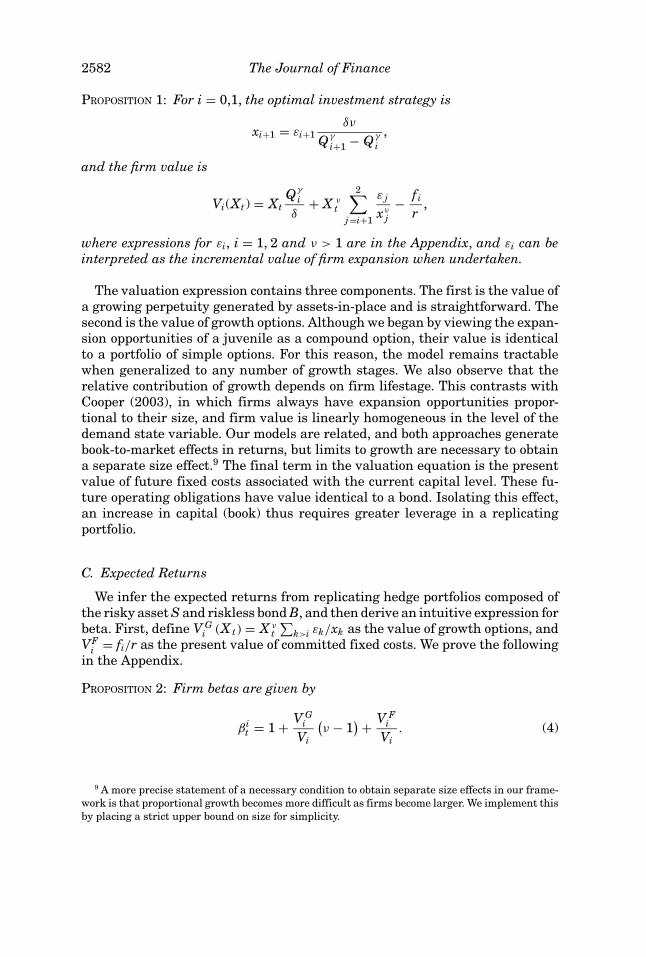
PROPOSITION 1: For i = 0,1, the optimal investment strategy is

xi+1 = εi+1δν

Qγ

i+1 − Qγ

i,

and the firm value is

Vi(Xt) = XtQγ

i

δ+ X ν

t

2∑j=i+1

ε j

xνj

− fi

r,

where expressions for εi, i = 1, 2 and ν > 1 are in the Appendix, and εi can beinterpreted as the incremental value of firm expansion when undertaken.

The valuation expression contains three components. The first is the value ofa growing perpetuity generated by assets-in-place and is straightforward. Thesecond is the value of growth options. Although we began by viewing the expan-sion opportunities of a juvenile as a compound option, their value is identicalto a portfolio of simple options. For this reason, the model remains tractablewhen generalized to any number of growth stages. We also observe that therelative contribution of growth depends on firm lifestage. This contrasts withCooper (2003), in which firms always have expansion opportunities propor-tional to their size, and firm value is linearly homogeneous in the level of thedemand state variable. Our models are related, and both approaches generatebook-to-market effects in returns, but limits to growth are necessary to obtaina separate size effect.9 The final term in the valuation equation is the presentvalue of future fixed costs associated with the current capital level. These fu-ture operating obligations have value identical to a bond. Isolating this effect,an increase in capital (book) thus requires greater leverage in a replicatingportfolio.

C. Expected Returns

We infer the expected returns from replicating hedge portfolios composed ofthe risky asset S and riskless bond B, and then derive an intuitive expression forbeta. First, define V G

i (X t) = X νt∑

k>i εk/xk as the value of growth options, andVF

i = fi/r as the present value of committed fixed costs. We prove the followingin the Appendix.

PROPOSITION 2: Firm betas are given by

βit = 1 + V G

i

Vi

(ν − 1

) + V Fi

Vi. (4)

9 A more precise statement of a necessary condition to obtain separate size effects in our frame-work is that proportional growth becomes more difficult as firms become larger. We implement thisby placing a strict upper bound on size for simplicity.


The interpretation of this formula parallels our intuition from the valuationexpression in Proposition 1. The first term is the firm’s revenue beta, or theriskiness of unlevered assets in place. This value was previously normalizedto one.10 The second term captures the leverage effect from growth options.The ratio V G

i /Vi gives the percentage of firm value in growth, and ν − 1 > 0 isthe excess riskiness of growth relative to assets in place. The decomposition ofthe first two terms between assets in place and growth can also be observed byrewriting these as the weighted average VA

i /Vi + (V Gi /Vi)ν, where VA

i = Vi − V Gi

is the value of assets in place. Finally, the third term in the equation derivesfrom operating leverage. The quantity VF

i is the present value of future commit-ments associated with the previous capital investment. Such obligations couldinclude the fixed operating costs of a plant, wage contracts, and long-term sup-ply arrangements. Their effect on firm risk is identical to financial leverage,although the economic mechanism is distinct and can be related to physicalcapital and thus to book value.

The analysis of two special cases serves to further clarify the determinants ofexpected returns. First, consider a mature firm that has no growth options. Inthis case only operating leverage affects the return beta, and β2

t = 1 + V F2 /V2.

Beta then monotonically decreases in firm value (for V2 > 0) and asymptoticallyapproaches one. Next, consider a firm that has no current cash flows, only oneoption to expand, and no postexpansion fixed costs. Beta is then constant atβ0

t = ν > 1 until the firm invests and drops to β1t = 1 after expansion.

D. Size and Book-to-Market Effects

Size and book-to-market are sufficient statistics for the underlying state vari-ables Xt and Kt. To verify this, observe that size (market value) and book-to-market uniquely identify book, or the installed capital level Kt. Holding thecapital-level constant, market value strictly increases in demand, allowing Xtto be recovered as well. The firm beta in equation (4) thus relates to observablesize and book-to-market characteristics.

We previously developed intuition suggesting that size in our model relates tothe ratio of growth options to assets in place, while book-to-market correspondsto operating leverage. This intuition is useful, but approximate. First, observethat the third term of equation (4) can be written as VF

i /Vi = r−1f (Ki)/Vi. Book-to-market thus describes the operating leverage component of risk up to a first-order approximation, and this characterization is complete when f (K) is lin-ear. Conditioning on book-to-market, the incremental information in size thenuniquely identifies the second component of equation (4), which is linear in theratio of growth options to assets-in-place.

Although closely related, the source of the size and book-to-market effects inour model is distinct from those in BGN and GKZ. In both of these previous mod-els, the value and riskiness of growth options do not vary across firms, and cross-sectional dispersion in beta is driven solely by differences in assets-in-place.

10 When the revenue beta is not one, it multiplies the entire right-hand side of equation (4).


0 2.5 5 7.5 10 12.5 150

500

1000

1500A: Firm Value

Xt

V(X

t)

3 3.5 4 4.5 5 5.5 6 6.5 7 7.51

1.5

2

2.5B: Beta vs. Size

ln(Vti)

β t

mature

adolescent

juvenile

mature adolescent

juvenile

x1 x

2

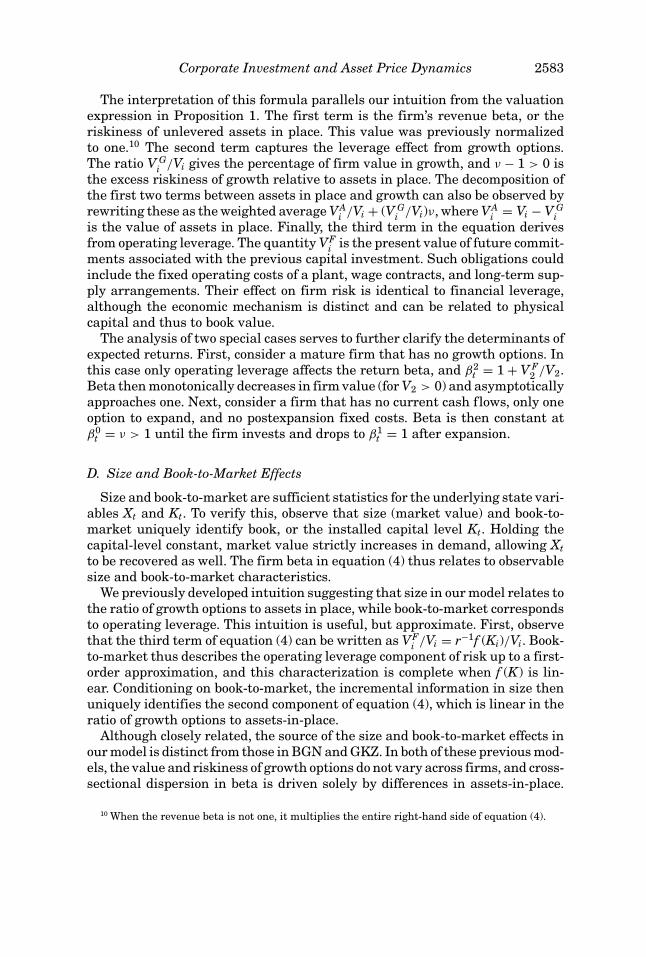
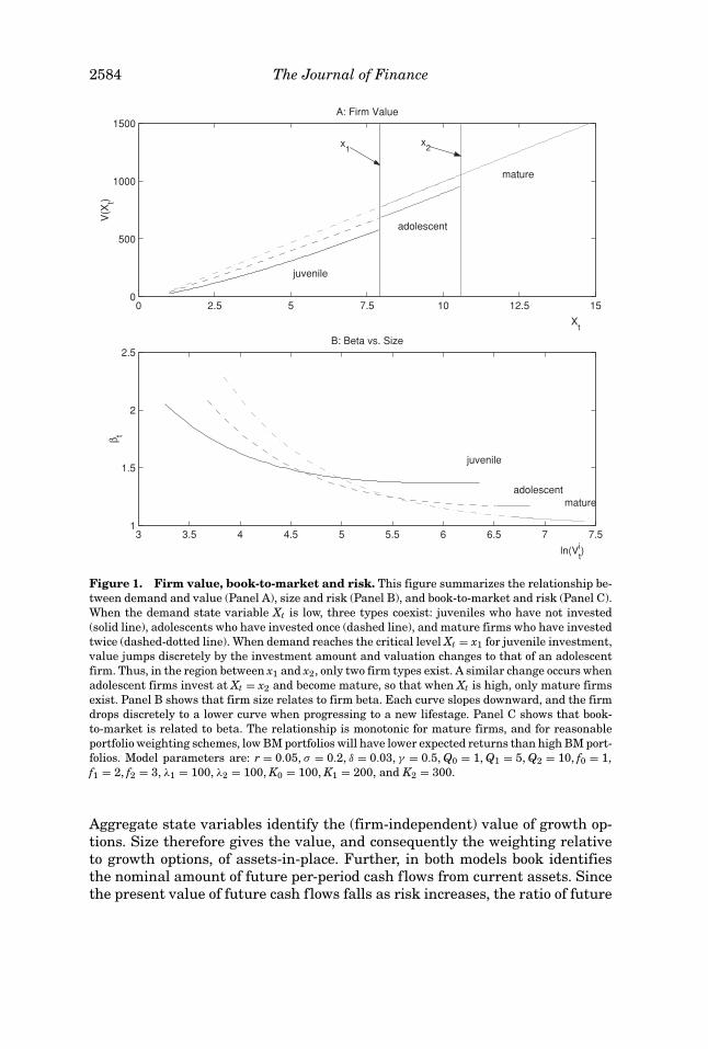
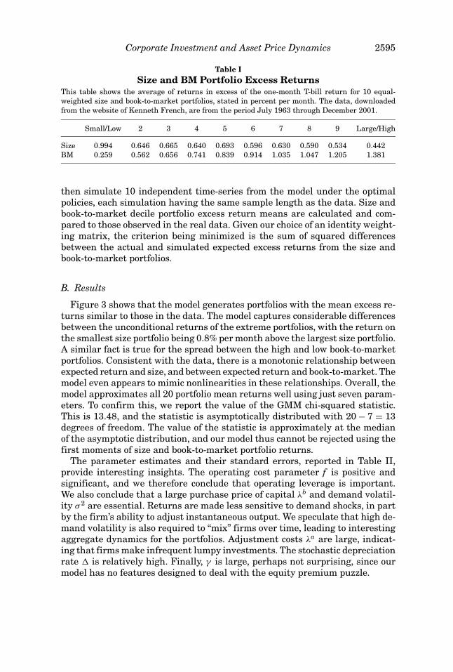
Figure 1. Firm value, book-to-market and risk. This figure summarizes the relationship be-tween demand and value (Panel A), size and risk (Panel B), and book-to-market and risk (Panel C).When the demand state variable Xt is low, three types coexist: juveniles who have not invested(solid line), adolescents who have invested once (dashed line), and mature firms who have investedtwice (dashed-dotted line). When demand reaches the critical level Xt = x1 for juvenile investment,value jumps discretely by the investment amount and valuation changes to that of an adolescentfirm. Thus, in the region between x1 and x2, only two firm types exist. A similar change occurs whenadolescent firms invest at Xt = x2 and become mature, so that when Xt is high, only mature firmsexist. Panel B shows that firm size relates to firm beta. Each curve slopes downward, and the firmdrops discretely to a lower curve when progressing to a new lifestage. Panel C shows that book-to-market is related to beta. The relationship is monotonic for mature firms, and for reasonableportfolio weighting schemes, low BM portfolios will have lower expected returns than high BM port-folios. Model parameters are: r = 0.05, σ = 0.2, δ = 0.03, γ = 0.5, Q0 = 1, Q1 = 5, Q2 = 10, f0 = 1,f1 = 2, f2 = 3, λ1 = 100, λ2 = 100, K0 = 100, K1 = 200, and K2 = 300.

Aggregate state variables identify the (firm-independent) value of growth op-tions. Size therefore gives the value, and consequently the weighting relativeto growth options, of assets-in-place. Further, in both models book identifiesthe nominal amount of future per-period cash flows from current assets. Sincethe present value of future cash flows falls as risk increases, the ratio of future


0 1 2 3 4 5 6 71

1.5

2

2.5C: Beta vs. Book–to–Market

Book–to–Market

β t

juvenile

adolescent mature

Figure 1.—Continued

cash flows (book) relative to their value (market) reveals the risk of assets inplace.11 Thus, an approximate intuition for BGN and GKZ is that size identifiesthe weighting of growth relative to assets-in-place, while book-to-market givesthe riskiness of assets-in-place.

Comparing these effects in BGN and GKZ with our model, we see that sizeplays a similar role in all three, and each has a critical assumption consistentwith empirical evidence that proportional growth becomes more difficult asmarket value increases. By contrast, the book-to-market effects in BGN andGKZ are different from those in our model. At some level, there is a commonality,as in all three cases book-to-market relates to the risk of assets-in-place. ForBGN and GKZ, however, this cross-sectional variation is driven by exogenousheterogeneity in the risks of previously accepted projects. Our model identifiesoperating leverage as a complementary economic mechanism. This is appealingbecause it applies even when projects are homogeneous in risk, and derives froman endogenous choice of scale.

Another interesting similarity between our model and the one in GKZ is thatboth size and book-to-market effects are generated with only one source of ag-gregate risk.12 Thus, if conditional beta were observable without error, size andbook-to-market would be redundant. In dynamic environments where measur-ing risk is difficult, these characteristics may nonetheless play an importantpractical role.

Figure 1 provides a numerical example of the size and book-to-market effectsin our model. Panel A relates firm value to the level of demand Xt for each pos-sible level of capital (and book value) Ki, i = 0, 1, 2. The lowest line in the panelcorresponds to the valuation function for a juvenile firm, and the highest is for

11 This intuition relates to arguments in Berk (1995).12 BGN focus on a model with two sources of aggregate risk, so conditional beta does not make

size and book-to-market redundant. In their special case with constant riskless rates, however,conditional beta is a sufficient statistic for risk and the above discussion applies.


a mature firm. Juvenile firm values are relevant only when Xt is between 0 andx1. For values larger than x1, the firm is either adolescent or mature, becausea juvenile firm will optimally invest as soon as demand reaches x1. Similarly,an adolescent firm optimally invests and becomes mature as soon as demandreaches x2. When investment occurs, the value of the firm jumps discretely, asnew equity is brought in to pay for new capital. The change in firm value isequal to the amount of new equity financing, preventing discontinuity in theshare price. Low values of the demand state variable Xt < x1 are compatiblewith any of the three capital levels. For example, a firm that once faced highdemand and invested must keep a high capital level even when demand de-creases, due to irreversible investment. Firm value monotonically increases indemand for any level of capital. This relationship is exactly linear for maturefirms, which have no remaining option value, and most nonlinear for juvenilefirms.

Figure 1 (Panel B) shows the relationship between firm value and beta. Fora given capital level, as firm value increases operating leverage drops, causingrisk to decrease. On the other hand, the proportion of growth options in totalfirm value also increases, causing risk to increase. For mature firms, only theoperating leverage effect is present and beta monotonically decreases in size.For juvenile and adolescent firms, the growth option effect becomes dominantin a small range just before investment occurs, when the relationship betweenfirm size and risk is reversed.

Focusing now on Panel C, firm risk monotonically increases in the book-to-market ratio for mature firms. Risk is generally increasing in book-to-marketfor juvenile and adolescent firms, but there is a small region of decreasingrisk for very low book-to-market ratios. Again, this corresponds to the re-gion just before the firm invests. Note that there is an independent size ef-fect: holding book-to-market constant, higher market values (mechanically,higher book values) are associated with the lower expected returns. This neednot necessarily be the case (e.g., Cooper (2003)). Limitations on the growthoptions of firms are sufficient to deliver separate size and book-to-marketeffects.

Our model thus provides an appealing economic intuition for size and book-to-market effects. In a partial equilibrium setting, finite growth opportunities andoperating leverage generate these effects in a model with closed-form solutions.The simple model developed in this section can now serve as the basis for astationary dynamic model that is empirically implementable.

II. A Model with Stationary Dynamics

This section relaxes some of the restrictive assumptions that are necessary toyield closed-form solutions, but retains the economics driving expected returns.We consider optimal production, investment, and shutdown policies for a value-maximizing all-equity firm in a discrete-time, infinite horizon setting. The firmfaces stochastic demand and adjustment costs in capital accumulation. The firmis again assumed to be a monopolist, which abstracts from strategic competition


in the product market and allows us to focus our analysis on the financialmarket for the firm’s securities.

By modeling a monopolist, we differ from Zhang (2003) and avoid the dif-ficult step of determining competitive goods market prices. The benefit of ourapproach is a significant reduction in computational complexity. This is of prac-tical importance, since our goal is to estimate this model using the simulatedmethod of moments, a process that requires the model to be solved hundreds oftimes. One limitation is that different goods are implicitly assumed to be nei-ther compliments nor substitutes. This makes extending the model to generalequilibrium a potentially difficult but interesting issue for the future research.

A. Demand Dynamics

We specify our model in discrete time so that it can be taken directly to thedata. During each period t = 1, 2, . . . , the monopolist faces downward slopinginverse demand,

Pt = Dt − bQt .

The intercept Dt is stochastic, the slope b is a fixed parameter, and Pt and Qtspecify price and quantity, respectively. We further specify

ln(Dt) = αXt + (1 − α)Zt . (5)

The state variable Xt reflects aggregate demand conditions that affect all firms,while Zt is firm-specific. (We defer indexing Zt by firm until we consider a cross-section in Section IV.) We restrict X and Z to have constant variances σx andσz. The logarithmic specification in equation (5) then ensures that demandgrowth has constant variance as well. Thus, any size effects that arise will beendogenous.

Section I highlighted the importance of limits to growth in generating sep-arate size and book-to-market effects. We now seek to achieve the same effectin a model with stationary dynamics that can be taken to the data. There areseveral ways to accomplish this. We choose a very simple specification withdemand state variables, Xt and Zt, assumed to be random walks without drifton a finite lattice.13 This is a convenient way of capturing the empirical evi-dence that larger firms have fewer growth opportunities (Evans (1987), Hall(1987)).14

B. Production and Capital Accumulation

The firm may produce one unit of output in each period for each unit ofcapital, with free disposal, giving 0 ≤ Qt ≤ Kt. For simplicity and without loss

13 When step size and lattice increments go to zero at appropriate rates, sequences of theseprocesses weakly converge to a Brownian motion with reflecting barriers.

14 We also implemented a specification that combined AR(1) dynamics with reflecting barriers,and found the autoregressive parameter to be insignificant.


of generality, we assume zero marginal costs of production. Operating leverageis introduced by assuming that in each period the firm pays a fixed cost of fper unit of currently outstanding capital. Thus, the current capital level affectsoperating cash flows both through a direct effect on fixed costs and through anindirect effect on output.

Current investment It affects the one period ahead capital level, and there isno depreciation. Thus,

Kt+1 = Kt + It . (6)

The firm can buy or sell capital at any time for a cost of λb per unit whenbuying, and a price of λs per unit when selling. It is thus natural to view λbKtas book value. When the firm changes the size of its capital stock, it also paysan adjustment cost λa. This amount is the same whether the firm is investingor disinvesting, and is independent of the size of the investment. Investmentrelated costs in period t are thus

λ (It) =

λa + λbIt if It > 0λa + λs It if It < 0

0 if It = 0.

Note that when −∞ < λs < λb, investment is reversible at some implicit cost.Hopenhayn (1992) and Ericson and Pakes (1995) make similar assumptions inrelated settings.

We require a minimum capital level k for active firms. This prevents “moth-balling” at zero capital and costlessly waiting for demand to improve. An al-ternative is to have an additional fixed operating cost that is independent ofcapital. These approaches are essentially equivalent, requiring ongoing expen-ditures to maintain exclusive access to a product market. We set the level ofk equal to the static optimal output for a firm at the minimum demand level,thereby avoiding the need to estimate an additional parameter.

C. Limited Liability and Shutdown

To reflect limited liability, the firm chooses ζt = 1 to continue operations andζt = 0 to shut down. The decision to shut down is irreversible, results in a firmvalue of zero, and is tracked by a state variable,

Y0 = 1, Yt = Yt−1ζt . (7)

Transition to the shutdown state may also result from stochastic obsolescence.This is assumed to occur with probability e−� per period.

D. The Pricing Kernel

We assume a stochastic discount factor {mt} that follows

mt+1 = mt exp[−r − γ (X t+1 − Et X t+1)],


where r and γ are positive constants. This pricing kernel captures the intuitionthat states associated with positive shocks are more heavily discounted thanthose associated with negative shocks. Unlike in BGN, there is no predictablevariation in this specification, and our pricing kernel does not admit a stochasticriskless interest rate or a time-varying risk premium. Our specification is closerto Zhang (2003), but more parsimonious in that the level of the state variableplays no role.15

III. Optimal Firm Policies and Valuation

We now define the optimal policies and derive firm value in different states.It is useful to distinguish between the economy-wide state variable Xt and thefirm-level state variables Zt, Kt, and Yt−1. The firm-level state space can be par-titioned into active states SA ≡ {Zt , Kt , Yt−1 : Yt−1 = 1} and a single absorbingstate SD for defunct firms with Yt−1 = 0.

A. The Static Production Decision

The unconstrained optimal quantity for the firm is Q∗t = Dt/2b. Given

its production constraints, the firm chooses Qt = min[Q∗, Kt] with operatingprofits

π (Dt , Kt) = Qt[Dt − bQt] − f Kt .

Operating profits do not include fixed adjustment costs or asset purchases andsales.

B. Firm Value and the Investment Decision

We first define feasible strategies in investment and the shutdown policy,which are for any St ∈ SA mappings

I : {Xt , St} → [k¯

− Kt , ∞)

ζ : {Xt , St} → {0, 1}.Firm value is

V (Xt , St) ≡ maxI (·),ζ (·)

Et

[ ∞∑τ=t

e−�mτ

mtC (Iτ , ζτ ; X τ , Sτ )

], (8)

where

C(It , ζt ; X t , St) = [π (Dt , Kt) − λ(It)]Yt−1ζt

15 Level effects in the state variable are used in Zhang (2003) to generate predictable variationin risk premia. This allows further study of the relation between business cycles and the valuepremium.


is the single period cash flow. The Bellman equation is

V (Xt , St) = maxIt ,ζt

Et

[C(It , ζt ; X t , St) + e−�mt+1

mtV (X t+1, St+1)

],

subject to the demand specification (5), capital accumulation (6), shutdownirreversibility (7), and transition equations for the state variables X and Z.

C. Optimal Investment and Shutdown

To describe optimal policies, it is convenient to define two mappings from{Xt, Zt} into target values of Kt+1. For i ∈ {b, s}, define the target capital levels

K i(Xt , Zt) ≡ argmaxKt+1

{Et

[e−�mt+1

mtV (X t+1, Zt+1, Kt+1, 1)

]− λi Kt+1

}.

These two functions give the optimal capital level at unit prices of λb and λs,respectively, ignoring fixed adjustment costs. The levels K b and Ks are inde-pendent of Kt and depend only on the demand state variables Zt and Xt. Weknow that if the firm chooses to pay fixed adjustment costs λa, it will optimallymove to one of these two capital levels.

We now determine whether the firm will pay the fixed adjustment cost andchange its capital level. The continuation value of the firm is

V (X t , Zt , K ) ≡ Et

[e−�mt+1

mtV (Xt+1, Zt+1, K , 1)

].

The firm will buy capital if K b(Xt, Zt) > Kt and

V(X t , Zt , K b(X t , Zt)

) − λ(K b(X t , Zt) − Kt

)> V (X t , Zt , Kt).

The firm will sell capital if Ks(Xt, Zt) < Kt and

V(X t , Zt , K s(X t , Zt)

) − λ(K s(X t , Zt) − Kt

)> V (X t , Zt , Kt).

Denote the triplets of (Xt, Zt, Kt) for which the firm buys capital by b and thosefor which it sells by s. Also denote the boundaries of these regions by φb andφs, respectively. The optimal investment policy I is now

I (Xt , Zt , Kt) =

K b(Xt , Zt) − Kt if (X t , Zt , Kt) ∈ b

K s(Xt , Zt) − Kt if (X t , Zt , Kt) ∈ s

0 otherwise.

The firm chooses to shut down (ζt = 0) if and only if

π (Dt , Kt) − λ(I (Xt , Zt , Kt))

+ Et

[e−�mt+1

mtV (Xt+1, Zt+1, Kt + I (Xt , Zt , Kt), 1)

]< 0.


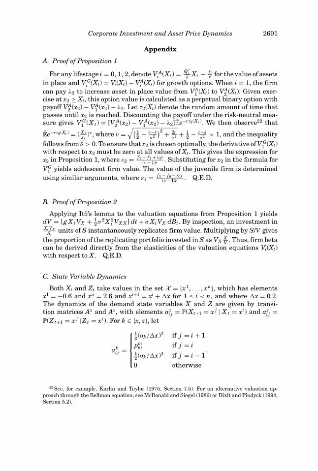
shutdown

Capital

Demand

Kb

Ks

φs

φb

XA XB XCXD

KA

KB

KC

KD

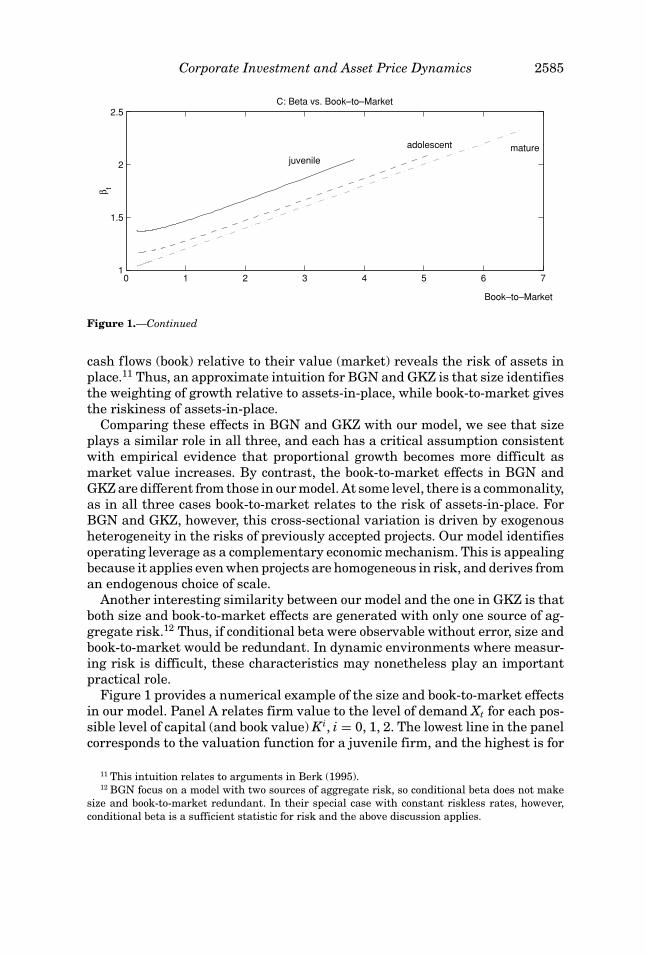
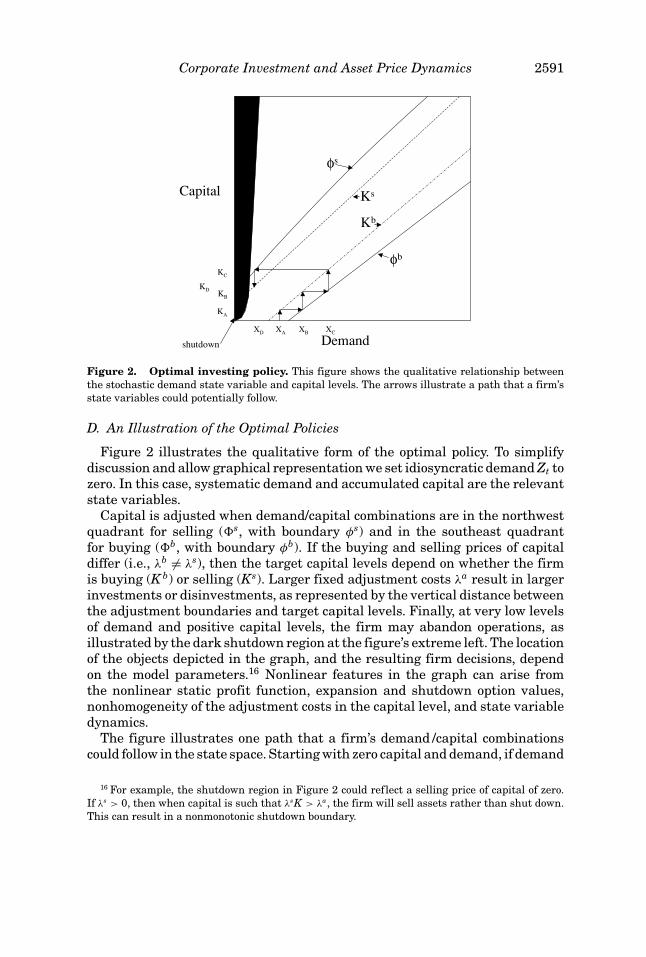
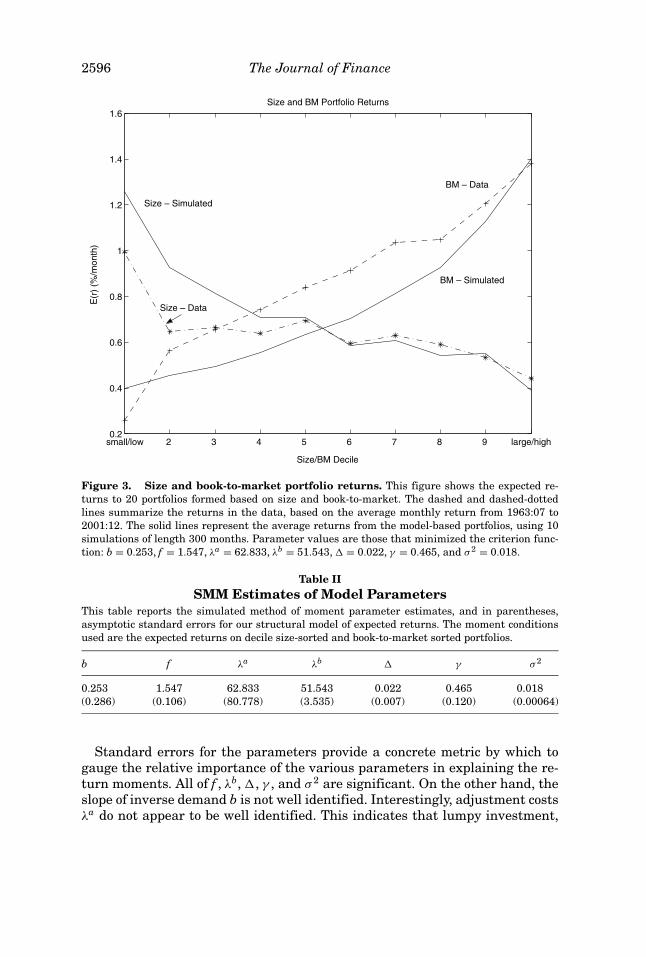
Figure 2. Optimal investing policy. This figure shows the qualitative relationship betweenthe stochastic demand state variable and capital levels. The arrows illustrate a path that a firm’sstate variables could potentially follow.

D. An Illustration of the Optimal Policies

Figure 2 illustrates the qualitative form of the optimal policy. To simplifydiscussion and allow graphical representation we set idiosyncratic demand Zt tozero. In this case, systematic demand and accumulated capital are the relevantstate variables.

Capital is adjusted when demand/capital combinations are in the northwestquadrant for selling ( s, with boundary φs) and in the southeast quadrantfor buying ( b, with boundary φb). If the buying and selling prices of capitaldiffer (i.e., λb �= λs), then the target capital levels depend on whether the firmis buying (K b) or selling (Ks). Larger fixed adjustment costs λa result in largerinvestments or disinvestments, as represented by the vertical distance betweenthe adjustment boundaries and target capital levels. Finally, at very low levelsof demand and positive capital levels, the firm may abandon operations, asillustrated by the dark shutdown region at the figure’s extreme left. The locationof the objects depicted in the graph, and the resulting firm decisions, dependon the model parameters.16 Nonlinear features in the graph can arise fromthe nonlinear static profit function, expansion and shutdown option values,nonhomogeneity of the adjustment costs in the capital level, and state variabledynamics.

The figure illustrates one path that a firm’s demand /capital combinationscould follow in the state space. Starting with zero capital and demand, if demand

16 For example, the shutdown region in Figure 2 could reflect a selling price of capital of zero.If λs > 0, then when capital is such that λsK > λa, the firm will sell assets rather than shut down.This can result in a nonmonotonic shutdown boundary.


increases to XA, then capital of KA will be bought. If demand increases furtherto XB, a second expansion from KA to KB takes place. Further investment will beundertaken whenever the investing boundary is reached. Conversely, if demandfalls from XC, there will be no adjustment until demand falls to XD. At that pointthe physical plant is reduced from KC to KD as the firm sells capital.

IV. Aggregate Economy Dynamics

Having solved the dynamic optimization problem of a single firm, we generatethe return dynamics of a cross-section of firms and estimate the model usingmoments of the data. The economy consists of a continuum of monopolistic firmsdistributed over the firm-level state space. Each faces the demand dynamicsset out in Sections II and III. In particular, the demand for each monopolist’sproduct is affected by the common systematic component Xt. Indexing the firmsby i, each firm has an independent and identically distributed idiosyncraticcomponent to their demand, given by Z i

t . Each of the firms makes independentdecisions about its optimal investment I i

t and hence the level of its capital stockK i

t+1.

A. Entry

Our model incorporates exit through limited liability and shutdown or ob-solescence. Since shutdown is irreversible, we must also permit entry or therewould eventually be no firms. We take a simple but economically intuitive ap-proach, which is to assume that entry opportunities are created by the exitof existing firms. We represent firms as infinitesimals, and while the mass ofpreviously shut down firms accumulates stochastically, the combined mass ofactive firms and potential entrants is held constant. This assumption is appro-priate for an economy with fixed investment opportunities.

A.1. Potential Entrants

To formalize this approach, let

SE ≡ {Zt , Kt , Yt−1 : Zt ∈ X , Kt = 0, Yt−1 = 1}be the partition of the firm-level state space reserved for new entrants. We notethat potential entrants are the only firms permitted to have zero capital.

Firms must belong to one of the three partitions corresponding to activeincumbent states SA, previously shutdown states SD, and potential entrantstates SE . Let S∗ denote the union of these partitions, and for any s ⊆ S∗, letψ∗

t (s) denote the measure of firms in states belonging to s at date t.Firms that exit prior to any date t are not relevant to the cross-section of

future returns. Thus, define S ≡ SA ∪ SE , and let ψt denote the restrictionof the measure ψ∗

t to S. Imposing that the measure of active firms and po-tential entrants is constant over time, and for convenience normalizing this


level to unity, we have ψt (S) = 1 for all t ≥ 0. The mass of potential entrantscan now be determined by the mass of active firms at the end of the previousperiod

ψt(SE ) = 1 − ψt(SA). (9)

Each potential entrant is given an independent draw for its idiosyncratic de-mand level Z i

t from the unconditional distribution of Z. Thus, for any idiosyn-cratic demand level z, potential entrants are fully characterized by ψt(Z i

t = z,K i

t = 0) = P(Z = z)ψt(SE ).

A.2. The Entry Decision

Each potential entrant has a single opportunity to begin operations. A firmthat does not enter is assigned the abandonment value of zero, and in the nextperiod a new potential entrant takes its place. There is thus no option valuein waiting to enter. The model could be extended to accommodate this featurewithout difficulty, but we seek to keep the entry decision as simple as possible,since our concern in this paper is about the cross-section of returns for publiclytraded firms.

The firm enters with capital level K b(Xt, Z it ) if

Et

[e−�mt+1

mtV

(Xt+1, Z i

t+1, K b(Xt , Z it

))] − λbK b(Xt , Z it

) − λa ≥ 0.

This requires that firm value upon entry exceed the cost of purchasing newcapital plus fixed adjustment costs.

B. Simulating the Cross-section of Returns

Aggregate economy transition dynamics are now fully specified, subject toinitial conditions. The risks in the firm-level state variables Z i

t integrate outcompletely due to our assumption that each firm is of infinitesimal size. Theprocess {Xt} is thus the only exogenous state variable at the aggregate level.The distribution of firms ψt summarizes information relevant to the currentand future cross-section of returns that derives from the initial distribution ψ0as well as the history X0, . . . , Xt−1 of demand. The aggregate state variables arethus Xt and the measure ψt on the firm-level state space S.

Assume initial conditions (X0, ψ0) where X 0 ∈ X and ψ0 is a measure onS satisfying ψ0 (S) = 1. The dynamics of {Xt} are first-order Markov and theAppendix shows that ψt+1 is fully determined by ψt and Xt, updated recursively.By then combining the time-series of firm cross-sections with numerically de-termined expected returns, calculated using the value function, portfolios canbe formed and returns generated for any given set of model parameters.


V. Empirical Implementation

A. Methodology

We estimate the model using simulated method of moments, as in Ingram andLee (1991) and Duffie and Singleton (1993). Our estimator can also be viewed asa special case of indirect inference (Gourieroux, Monfort, and Renault (1993)).An excellent discussion of these methods is in Gourieroux, Renault, and Touzi(2000).

The procedure is described in the Appendix, and we outline it here. Estimatesof a vector θ0 of true model parameters are desired. Given a candidate vector,data are simulated, and a set of moments is calculated. An objective function isused to compare these moments to those in the data, and the parameter vectoris updated to improve the fit. The simulated method of moments estimatorminimizes the objective function.

In order to keep the estimation computationally tractable and to aid in iden-tification, it is necessary to place a priori restrictions on some parameters andto estimate others. In deciding which parameters to estimate, we are guidedby our primary motivation to understand how lumpy investment options, irre-versibility, and operating leverage interact to generate return characteristics.Hence, we estimate the level f of fixed operating costs per unit capital, thefixed cost λa of capital adjustment, and the per-unit purchase price λb of capi-tal. The option to invest is also driven by the variance of both systematic andidiosyncratic demand shocks. We estimate σ 2 ≡ σ 2

z = σ 2x to capture this effect

in a parsimonious manner. We also estimate the demand parameter b becauseit provides a role for operating flexibility, which should affect operating lever-age. Finally, we estimate �, the rate of stochastic obsolescence, and γ , whichdetermines risk premia.

The remaining parameters are fixed. The model roughly scales in costs anddemands, and since we estimate several cost parameters, upper and lowerboundaries for X and Z are imposed exogenously.17 We also set the system-atic proportion of demand to be α = 0.5. We let r = 0.005 in order to yield areasonable riskless interest rate. Finally, to capture the intuition that someirreversibility in investment is economically relevant, we fix λs = 0. We thusestimate a restricted version of the model with a vector

θ = [b, f , λa, λb, �, γ , σ 2]

of seven parameters.We use as moment conditions the mean return on decile portfolios of size-

sorted and book-to-market-sorted returns. The data are for the period July1963 through December 2001.18 Table I provides summary statistics for thesereturns. Following Cochrane (1996), we choose an identity weighting matrix.

Recalling the specific estimation strategy, for each potential set of parame-ters, optimal Markov investment policies under the model are calculated. We

17 The Appendix describes the lattice for these state variables.18 These data were downloaded from the Website of Kenneth French.


Table ISize and BM Portfolio Excess Returns

This table shows the average of returns in excess of the one-month T-bill return for 10 equal-weighted size and book-to-market portfolios, stated in percent per month. The data, downloadedfrom the website of Kenneth French, are from the period July 1963 through December 2001.

Small/Low 2 3 4 5 6 7 8 9 Large/High

Size 0.994 0.646 0.665 0.640 0.693 0.596 0.630 0.590 0.534 0.442BM 0.259 0.562 0.656 0.741 0.839 0.914 1.035 1.047 1.205 1.381

then simulate 10 independent time-series from the model under the optimalpolicies, each simulation having the same sample length as the data. Size andbook-to-market decile portfolio excess return means are calculated and com-pared to those observed in the real data. Given our choice of an identity weight-ing matrix, the criterion being minimized is the sum of squared differencesbetween the actual and simulated expected excess returns from the size andbook-to-market portfolios.

B. Results

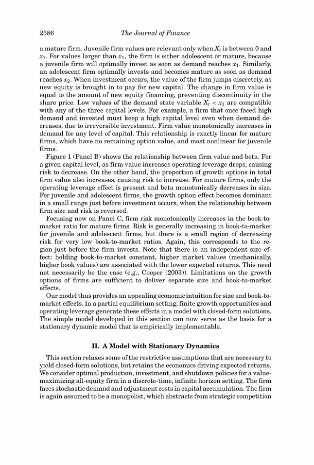
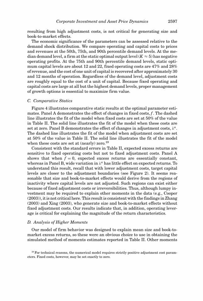
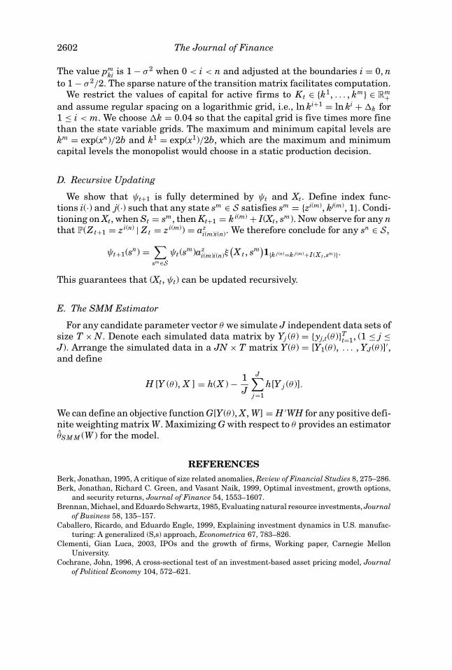
Figure 3 shows that the model generates portfolios with the mean excess re-turns similar to those in the data. The model captures considerable differencesbetween the unconditional returns of the extreme portfolios, with the return onthe smallest size portfolio being 0.8% per month above the largest size portfolio.A similar fact is true for the spread between the high and low book-to-marketportfolios. Consistent with the data, there is a monotonic relationship betweenexpected return and size, and between expected return and book-to-market. Themodel even appears to mimic nonlinearities in these relationships. Overall, themodel approximates all 20 portfolio mean returns well using just seven param-eters. To confirm this, we report the value of the GMM chi-squared statistic.This is 13.48, and the statistic is asymptotically distributed with 20 − 7 = 13degrees of freedom. The value of the statistic is approximately at the medianof the asymptotic distribution, and our model thus cannot be rejected using thefirst moments of size and book-to-market portfolio returns.

The parameter estimates and their standard errors, reported in Table II,provide interesting insights. The operating cost parameter f is positive andsignificant, and we therefore conclude that operating leverage is important.We also conclude that a large purchase price of capital λb and demand volatil-ity σ 2 are essential. Returns are made less sensitive to demand shocks, in partby the firm’s ability to adjust instantaneous output. We speculate that high de-mand volatility is also required to “mix” firms over time, leading to interestingaggregate dynamics for the portfolios. Adjustment costs λa are large, indicat-ing that firms make infrequent lumpy investments. The stochastic depreciationrate � is relatively high. Finally, γ is large, perhaps not surprising, since ourmodel has no features designed to deal with the equity premium puzzle.


small/low 2 3 4 5 6 7 8 9 large/high0.2

0.4

0.6

0.8

1

1.2

1.4

1.6

Size/BM Decile

E(r

) (%

/mon

th)

Size and BM Portfolio Returns

BM – Data

BM – Simulated

Size – Simulated

Size – Data

Figure 3. Size and book-to-market portfolio returns. This figure shows the expected re-turns to 20 portfolios formed based on size and book-to-market. The dashed and dashed-dottedlines summarize the returns in the data, based on the average monthly return from 1963:07 to2001:12. The solid lines represent the average returns from the model-based portfolios, using 10simulations of length 300 months. Parameter values are those that minimized the criterion func-tion: b = 0.253, f = 1.547, λa = 62.833, λb = 51.543, � = 0.022, γ = 0.465, and σ 2 = 0.018.

Table IISMM Estimates of Model Parameters

This table reports the simulated method of moment parameter estimates, and in parentheses,asymptotic standard errors for our structural model of expected returns. The moment conditionsused are the expected returns on decile size-sorted and book-to-market sorted portfolios.

b f λa λb � γ σ 2

0.253 1.547 62.833 51.543 0.022 0.465 0.018(0.286) (0.106) (80.778) (3.535) (0.007) (0.120) (0.00064)

Standard errors for the parameters provide a concrete metric by which togauge the relative importance of the various parameters in explaining the re-turn moments. All of f , λb, �, γ , and σ 2 are significant. On the other hand, theslope of inverse demand b is not well identified. Interestingly, adjustment costsλa do not appear to be well identified. This indicates that lumpy investment,


resulting from high adjustment costs, is not critical for generating size andbook-to-market effects.

The economic significance of the parameters can be assessed relative to thedemand shock distribution. We compare operating and capital costs to pricesand revenues at the 50th, 75th, and 90th percentile demand levels. At the me-dian demand level, a firm at the static optimal output level (K ≈ 5) has negativeoperating profits. At the 75th and 90th percentile demand levels, static opti-mum capital levels are about 12 and 22, fixed operating costs are 47% and 28%of revenue, and the cost of one unit of capital is recovered after approximately 30and 12 months of operation. Regardless of the demand level, adjustment costsare roughly equal to the cost of a unit of capital. Because fixed operating andcapital costs are large at all but the highest demand levels, proper managementof growth options is essential to maximize firm value.

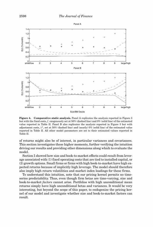
C. Comparative Statics

Figure 4 illustrates comparative static results at the optimal parameter esti-mates. Panel A demonstrates the effect of changes in fixed costs, f . The dashedline illustrates the fit of the model when fixed costs are set at 50% of the valuein Table II. The solid line illustrates the fit of the model when these costs areset at zero. Panel B demonstrates the effect of changes in adjustment costs, λa.The dashed line illustrates the fit of the model when adjustment costs are setat 50% of the value in Table II. The solid line illustrates the fit of the modelwhen these costs are set at (nearly) zero.19

Consistent with the standard errors in Table II, expected excess returns aresensitive to fixed operating costs but not to fixed adjustment costs. Panel Ashows that when f = 0, expected excess returns are essentially constant,whereas in Panel B, wide variation in λa has little effect on expected returns. Tounderstand this result, recall that with lower adjustment costs, target capitallevels are closer to the adjustment boundaries (see Figure 2). It seems rea-sonable that size and book-to-market effects would derive from the regions ofinactivity where capital levels are not adjusted. Such regions can exist eitherbecause of fixed adjustment costs or irreversibilities. Thus, although lumpy in-vestment may be required to explain other moments in the data (e.g., Cooper(2003)), it is not critical here. This result is consistent with the findings in Zhang(2003) and Xing (2003), who generate size and book-to-market effects withoutfixed adjustment costs. Our results indicate that, in addition, operating lever-age is critical for explaining the magnitude of the return characteristics.

D. Analysis of Higher Moments

Our model of firm behavior was designed to explain mean size and book-to-market excess returns, so these were an obvious choice to use in obtaining thesimulated method of moments estimates reported in Table II. Other moments

19 For technical reasons, the numerical model requires strictly positive adjustment cost param-eters. Fixed costs, however, may be set exactly to zero.


small/low 2 3 4 5 6 7 8 9 large/high0

0.2

0.4

0.6

0.8

1

1.2

1.4

Panel B

Size/BM Decile

E(r

) (%

/mon

th)

small/low 2 3 4 5 6 7 8 9 large/high0

0.2

0.4

0.6

0.8

1

1.2

1.4

Panel AE

(r)

(%/m

onth

)

Figure 4. Comparative static analysis. Panel A replicates the analysis reported in Figure 3but with the fixed costs, f , exogenously set at 50% (dashed line) and 0% (solid line) of the estimatedvalue reported in Table II. Panel B also replicates the analysis reported in Figure 3 but withadjustment costs, λa, set at 50% (dashed line) and (nearly) 0% (solid line) of the estimated valuereported in Table II. All other model parameters are set to their estimated values reported inTable II.

of returns might also be of interest, in particular variances and covariances.This section investigates these higher moments, further verifying the intuitiondriving our results and providing other dimensions along which to evaluate themodel.

Section I showed how size and book-to-market effects could result from lever-age associated with (1) fixed operating costs that are tied to installed capital, or(2) growth options. Small firms or firms with high book-to-market have high ex-pected returns because of implicitly high leverage. The model should thereforealso imply high return volatilities and market index loadings for these firms.

To understand this intuition, note that our pricing kernel permits no time-series predictability. Thus, even though firm betas are time-varying, size andbook-to-market factors cannot arise. Portfolios with high unconditional meanreturns simply have high unconditional betas and variances. It would be veryinteresting, but beyond the scope of this paper, to endogenize the pricing ker-nel of our model and investigate whether size and book-to-market factors canresult.


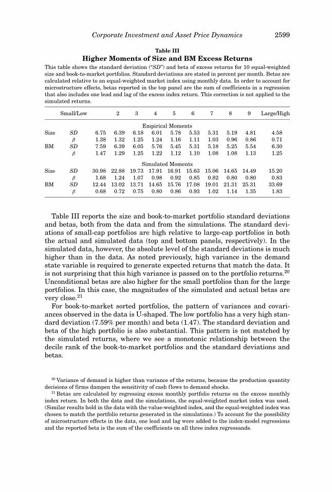
Table IIIHigher Moments of Size and BM Excess Returns

This table shows the standard deviation (“SD”) and beta of excess returns for 10 equal-weightedsize and book-to-market portfolios. Standard deviations are stated in percent per month. Betas arecalculated relative to an equal-weighted market index using monthly data. In order to account formicrostructure effects, betas reported in the top panel are the sum of coefficients in a regressionthat also includes one lead and lag of the excess index return. This correction is not applied to thesimulated returns.

Small/Low 2 3 4 5 6 7 8 9 Large/High

Empirical MomentsSize SD 6.75 6.39 6.18 6.01 5.78 5.53 5.31 5.19 4.81 4.58

β 1.38 1.32 1.25 1.24 1.16 1.11 1.03 0.96 0.86 0.71BM SD 7.59 6.39 6.05 5.76 5.45 5.31 5.18 5.25 5.54 6.30

β 1.47 1.29 1.25 1.22 1.12 1.10 1.08 1.08 1.13 1.25

Simulated MomentsSize SD 30.98 22.88 19.73 17.91 16.91 15.63 15.06 14.65 14.49 15.20

β 1.68 1.24 1.07 0.98 0.92 0.85 0.82 0.80 0.80 0.83BM SD 12.44 13.02 13.71 14.65 15.76 17.08 19.01 21.31 25.31 33.69

β 0.68 0.72 0.75 0.80 0.86 0.93 1.02 1.14 1.35 1.83

Table III reports the size and book-to-market portfolio standard deviationsand betas, both from the data and from the simulations. The standard devi-ations of small-cap portfolios are high relative to large-cap portfolios in boththe actual and simulated data (top and bottom panels, respectively). In thesimulated data, however, the absolute level of the standard deviations is muchhigher than in the data. As noted previously, high variance in the demandstate variable is required to generate expected returns that match the data. Itis not surprising that this high variance is passed on to the portfolio returns.20

Unconditional betas are also higher for the small portfolios than for the largeportfolios. In this case, the magnitudes of the simulated and actual betas arevery close.21

For book-to-market sorted portfolios, the pattern of variances and covari-ances observed in the data is U-shaped. The low portfolio has a very high stan-dard deviation (7.59% per month) and beta (1.47). The standard deviation andbeta of the high portfolio is also substantial. This pattern is not matched bythe simulated returns, where we see a monotonic relationship between thedecile rank of the book-to-market portfolios and the standard deviations andbetas.

20 Variance of demand is higher than variance of the returns, because the production quantitydecisions of firms dampen the sensitivity of cash flows to demand shocks.

21 Betas are calculated by regressing excess monthly portfolio returns on the excess monthlyindex return. In both the data and the simulations, the equal-weighted market index was used.(Similar results hold in the data with the value-weighted index, and the equal-weighted index waschosen to match the portfolio returns generated in the simulations.) To account for the possibilityof microstructure effects in the data, one lead and lag were added to the index-model regressionsand the reported beta is the sum of the coefficients on all three index regressands.


To summarize, when using the estimated parameters from Table II, the modelproduces size portfolio betas that are consistent with those found in the data.However, portfolio standard deviations are much too high. This result may berelated to our pricing kernel, which like many stochastic discount factors hasdifficulty addressing the equity premium puzzle. More difficult to explain arethe actual relationships between book-to-market portfolio standard deviationsand betas. The U-shaped pattern in these higher moments is not capturedby our current specification. It is interesting to speculate what other sourcesof return variation might be useful to help reproduce these features of thedata.

VI. Conclusion

We develop two models of the relation between expected returns and endoge-nous corporate investment decisions. We obtain a new economic explanation forthe book-to-market effect as driven by operating leverage. When demand for afirm’s product decreases, equity value falls relative to book value, which is equalto the size of the capital stock. With fixed operating costs that increase in thesize of the capital stock, risk rises due to higher operating leverage. The modelsalso highlight the importance of limits to proportional growth in generating asize effect.

Our first model supposes a firm-facing stochastic iso-elastic demand drivenby a lognormal diffusion. Firms have finite opportunities to irreversibly expandtheir capital base, and must pay fixed operating costs that vary with the level ofaccumulated capital. We derive closed-form expressions for expected returns,and show that the firm beta is linear in the ratio of growth opportunities toassets in place, as well as the ratio of fixed costs to total firm value. We then showthat book-to-market and size are sufficient statistics for operating leverage andthe ratio of growth opportunities to assets in place. We are thus able to relatesize and book-to-market effects to sensible economic causes in a single-factormodel with closed-form solutions.

The second model incorporates this basic intuition in a more realistic settingwith stationary dynamics. Our goal is to obtain a structural model that can beestimated using standard methods. We suppose that a cross-sectional contin-uum of monopolistic firms have demand dynamics composed of one commoncomponent, and that for each firm there is a unique idiosyncratic component.The common and idiosyncratic components are modeled as independent butstatistically identical stationary processes. We add realistic features, includingcapital adjustment costs, costly reversibility of investment, limited liability andshutdown, and entry. We find an optimal Markov strategy for each firm that is afunction of the common and idiosyncratic demand components and the existingcapital level of the firm. We estimate the model using the simulated method ofmoments. As moment conditions, we choose the mean excess returns on decilesize and book-to-market portfolios. We find that the estimation method workswell, and that the model accounts both qualitatively and quantitatively for thesize and book-to-market effects observed in the data.


Appendix

A. Proof of Proposition 1

For any lifestage i = 0, 1, 2, denote V Ai (Xt) = Qγ

iδ

Xt − fir for the value of assets

in place and V Gi (Xt) = Vi(Xt) − VA

i (Xt) for growth options. When i = 1, the firmcan pay λ2 to increase asset in place value from VA

1 (Xt) to VA2 (Xt). Given exer-

cise at x2 ≥ Xt, this option value is calculated as a perpetual binary option withpayoff VA

2 (x2) − VA1 (x2) − λ2. Let τ2(Xt) denote the random amount of time that

passes until x2 is reached. Discounting the payoff under the risk-neutral mea-sure gives V G

1 (X t) = [V A2 (x2) − V A

1 (x2) − λ2]Ee−rτ2(X t ). We then observe22 that

Ee−rτ2(Xt ) = ( X tx2

)ν , where ν =√( 1

2 − r−δ

σ 2

)2 + 2rσ 2 + 1

2 − r−δ

σ 2 > 1, and the inequalityfollows from δ > 0. To ensure that x2 is chosen optimally, the derivative of V G

1 (Xt)with respect to x2 must be zero at all values of Xt. This gives the expression forx2 in Proposition 1, where ε2 = f2 − f1 + λ2r

(ν − 1)r . Substituting for x2 in the formula forVG

1 yields adolescent firm value. The value of the juvenile firm is determinedusing similar arguments, where ε1 = f1 − f0 + λ1r

(ν − 1)r . Q.E.D.

B. Proof of Proposition 2

Applying Ito’s lemma to the valuation equations from Proposition 1 yieldsdV = [g X t VX + 1

2σ 2 X 2t VX X ] dt + σ Xt VX dBt . By inspection, an investment in

Xt VXSt

units of S instantaneously replicates firm value. Multiplying by S/V givesthe proportion of the replicating portfolio invested in S as VX

XV . Thus, firm beta

can be derived directly from the elasticities of the valuation equations Vi(Xt)with respect to X. Q.E.D.

C. State Variable Dynamics

Both Xt and Zt take values in the set X = {x1, . . . , xn}, which has elementsx1 = −0.6 and xn = 2.6 and xi+1 = xi + �x for 1 ≤ i < n, and where �x = 0.2.The dynamics of the demand state variables X and Z are given by transi-tion matrices Ax and Az, with elements ax

i j = P(Xt+1 = x j | X t = xi) and azi j =

P(Zt+1 = x j |Zt = xi). For k ∈ {x, z}, let

aki j =

12 (σk/�x)2 if j = i + 1pm

ki if j = i12 (σk/�x)2 if j = i − 10 otherwise

.

22 See, for example, Karlin and Taylor (1975, Section 7.5). For an alternative valuation ap-proach through the Bellman equation, see McDonald and Siegel (1986) or Dixit and Pindyck (1994,Section 5.2).


The value pmki is 1 − σ 2 when 0 < i < n and adjusted at the boundaries i = 0, n

to 1 − σ 2/2. The sparse nature of the transition matrix facilitates computation.We restrict the values of capital for active firms to Kt ∈ {k1, . . . , km} ∈ R

m+

and assume regular spacing on a logarithmic grid, i.e., ln ki+1 = ln ki + �k for1 ≤ i < m. We choose �k = 0.04 so that the capital grid is five times more finethan the state variable grids. The maximum and minimum capital levels arekm = exp(xn)/2b and k1 = exp(x1)/2b, which are the maximum and minimumcapital levels the monopolist would choose in a static production decision.

D. Recursive Updating

We show that ψt+1 is fully determined by ψt and Xt. Define index func-tions i(·) and j(·) such that any state sm ∈ S satisfies sm = {zi(m), kj(m), 1}. Condi-tioning on Xt, when St = sm, then Kt+1 = ki(m) + I(Xt, sm). Now observe for any nthat P(Zt+1 = zi(n) | Zt = zi(m)) = az

i(m)i(n). We therefore conclude for any sn ∈ S,

ψt+1(sn) =∑sm∈S

ψt(sm)azi(m)i(n)ξ

(X t , sm)

1{k j (n)=k j (m)+I (X t ,sm)}.

This guarantees that (Xt, ψt) can be updated recursively.

E. The SMM Estimator

For any candidate parameter vector θ we simulate J independent data sets ofsize T × N. Denote each simulated data matrix by Yj (θ ) = {yj,t(θ )}T

t=1, (1 ≤ j ≤J). Arrange the simulated data in a JN × T matrix Y(θ ) = [Y1(θ ), . . . , YJ(θ )]′,and define

H [Y (θ ), X ] = h(X ) − 1J

J∑j=1

h[Y j (θ )].

We can define an objective function G[Y(θ ), X, W] = H ′WH for any positive defi-nite weighting matrix W. Maximizing G with respect to θ provides an estimatorθSM M (W ) for the model.

REFERENCESBerk, Jonathan, 1995, A critique of size related anomalies, Review of Financial Studies 8, 275–286.Berk, Jonathan, Richard C. Green, and Vasant Naik, 1999, Optimal investment, growth options,

and security returns, Journal of Finance 54, 1553–1607.Brennan, Michael, and Eduardo Schwartz, 1985, Evaluating natural resource investments, Journal

of Business 58, 135–157.Caballero, Ricardo, and Eduardo Engle, 1999, Explaining investment dynamics in U.S. manufac-

turing: A generalized (S,s) approach, Econometrica 67, 783–826.Clementi, Gian Luca, 2003, IPOs and the growth of firms, Working paper, Carnegie Mellon

University.Cochrane, John, 1996, A cross-sectional test of an investment-based asset pricing model, Journal

of Political Economy 104, 572–621.


Cooper, Ilan, 2003, Asset pricing implications of non-convex adjustment costs of investment, Work-ing paper, Norwegian School of Management.

Daniel, Kent D., and Sheridan Titman, 1997, Evidence on the characteristics of cross sectionalvariation in stock returns, Journal of Finance 52, 572–621.

Dixit, Avinash K., and Robert S. Pindyck, 1994, Investment under Uncertainty (Princeton UniversityPress, Princeton).

Duffie, Darrell, and Kenneth Singleton, 1993, Simulated moments estimation of Markov modelsof asset prices, Econometrica 61, 929–952.

Ericson, Richard, and Ariel Pakes, 1995, Markov-perfect industry dynamics: A framework for em-pirical work, Review of Economic Studies 62, 53–82.

Evans, David, 1987, The relationship between firm growth, size, and age: Estimates for 100 man-ufacturing industries, Journal of Industrial Economics 35, 567–581.

Fama, Eugene, and Kenneth French, 1992, The cross-section of expected stock returns, Journal ofFinance 47, 427–465.

Fama, Eugene, and Kenneth French, 1993, Common risk factors in the returns on stocks and bonds,Journal of Financial Economics 33, 3–56.

Ferson, Wayne, and Campbell Harvey, 1999, Conditioning variables and the cross-section of stockreturns, Journal of Finance 54, 1325–1360.

Gomes, Joao, Leonid Kogan, and Lu Zhang, 2003, Equilibrium cross-section of returns, Journal ofPolitical Economy 111, 693–732.

Gomes, Joao, and Dmitry Livdan, 2002, Optimal diversification: Reconciling theory and evidence,Journal of Finance 59, 507–535.

Gourieroux, Christian, Alain Monfort, and Eric Renault, 1993, Indirect inference, Journal of Ap-plied Econometrics 8, S85–S118.

Gourieroux, Christian, Eric Renault, and Nizar Touzi, 2000, Calibration by simulation for smallsample bias correction, in Roberto Mariano, Til Schuermann, and Melvyn Weeks, eds.:Simulation-based Inference in Econometrics (Cambridge University Press, Cambridge, Mass).

Hall, Bronwyn H., 1987, The relationship between firm size and firm growth in the U.S. manufac-turing sector, Journal of Industrial Economics 35, 583–606.

Hansen, Lars, and Scott F. Richard, 1987, The role of conditioning information in deducing testablerestrictions implied by dynamic asset pricing models, Econometrica 55, 587–613.

Hopenhayn, Hugo A., 1992, Entry, exit, and firm dynamics in long run equilibrium, Econometrica60, 1127–1150.

Ingram, Beth F., and Bong-Soo Lee, 1991, Simulation estimation of time series models, Journal ofEconometrics 47, 197–205.

Jagannathan, Ravi, and Zhenyu Wang, 1996, The conditional CAPM and the cross-section of ex-pected returns, Journal of Finance 51, 3–53.

Johnson, Timothy C., 2002, Rational momentum effects, Journal of Finance 57, 585–608.Karlin, Samuel, and Howard M. Taylor, 1975, A First Course in Stochastic Processes, Second edition

(Academic Press, San Diego).McDonald, Robert, and Daniel Siegel, 1985, Investment and the valuation of firms when there is

an option to shut down, International Economic Review 26, 331–349.McDonald, Robert, and Daniel Siegel, 1986, The value of waiting to invest, Quarterly Journal of

Economics 101, 707–727.Xing, Yuhang, 2003, Firm investments and expected equity returns, Working paper, Columbia

University.Zhang, Lu, 2003, The value premium, Journal of Finance, forthcoming.

Documents

Corporate Investment and Asset Price Dynamics ...faculty.haas.berkeley.edu/garleanu/ReadingGroup_AP_Sp2012/Carlson... · Corporate Investment and Asset Price Dynamics: ... Robert