Asset price dynamics with heterogeneous groups

Physica D 225 (2007) 43–54www.elsevier.com/locate/physd

Asset price dynamics with heterogeneous groups

G. Caginalpa, H. Merdanb,∗

a Mathematics Department, University of Pittsburgh, Pittsburgh, PA 15260, USAb Mathematics Department, TOBB Economics and Technology University, Ankara, Turkey

Received 2 May 2006; accepted 28 September 2006Available online 17 November 2006

Communicated by Y. Nishiura

Abstract

A system of ordinary differential equations is used to study the price dynamics of an asset under various conditions. One of these involves theintroduction of new information that is interpreted differently by two groups. Another studies the price change due to a change in the number ofshares. The steady state is examined under these conditions to determine the changes in the price due to these phenomena. Numerical studies arealso performed to understand the transition between the regimes. The differential equations naturally incorporate the effects due to the finiteness ofassets (rather than assuming unbounded arbitrage) in addition to investment strategies that are based on either price momentum (trend) or valuationconsiderations. The numerical studies are compared with closed-end funds that issue additional shares, and offers insight into the strategies ofinvestors.c© 2006 Elsevier B.V. All rights reserved.

Keywords: Ordinary differential equations for asset pricing; Steady states of asset prices; Dynamical system approach to mathematical finance; Secondary issuesand stock buybacks; Closed-end funds

1. Introduction

Classical economics stipulates that an equilibrium price isattained when supply and demand are equal. The neoclassicalapproach to the dynamics of asset prices assumes that pricesreturn to equilibrium at a rate that is proportional to the extentto which they are out of equilibrium. There are three tacitassumptions in the classical and neoclassical descriptions ofasset prices: (i) the supply and demand are based upon the valueof the asset; (ii) there is a general agreement on the valuationof an asset among market participants since the information ispublic; and (iii) there is a huge amount of capital that wouldquickly take advantage of any discrepancies from a realisticvalue of the asset. While these classical academic theoriesare sometimes a useful idealization of asset market dynamics,they neglect several key aspects that are routinely examined bypractitioners.

∗ Corresponding author. Tel.: +90 312 2924146; fax: +90 312 2924326.E-mail addresses: [email protected] (G. Caginalp), [email protected]

(H. Merdan).

0167-2789/$ - see front matter c© 2006 Elsevier B.V. All rights reserved.doi:10.1016/j.physd.2006.09.036

First, it has been known for some time that diverse moti-vations underlie the buying and selling of shares. An impor-tant motivation is often due to the price trend that is evident totraders. Sometimes called the momentum effect, this has com-plex origins in terms of trader psychology and strategy. For ex-ample, it may be purely rational self-interest in the case of amoney manager who had previously minimized his portfolio ina sector where prices are rising rapidly. As his portfolio lagsthe averages, he would find it difficult to maintain his investors,or even his job, by ignoring the trend. The motivation couldbe regret avoidance on the part of an individual investor whodoes not want to sell a rising stock in anticipation of the regrethe would feel upon observing his stock at a higher price afterhe has sold it. As a stock is declining in price, the motivation tosell could arise in a purely rational way if the investor receives amargin call, i.e., the broker informs him that he must send morefunds to cover borrowed money to avoid liquidation of the po-sition, otherwise the position will be liquidated. Alternatively,the selling could arise from fear of further declines in price, orthe attempt to avoid the regret of not having sold sooner.

Secondly, the concept of a unique price determined by theset of all available information is an interesting idealization. It

http://www.elsevier.com/locate/physd

mailto:[email protected]

mailto:[email protected]

http://dx.doi.org/10.1016/j.physd.2006.09.036

44 G. Caginalp, H. Merdan / Physica D 225 (2007) 43–54

is based on the idea of each trader realizing that other tradersknow what he knows, etc. This game theoretic analysis isassumed to be iterated indefinitely and to lead to a unique fixedpoint. Of course this is an oversimplification both theoreticallyand practically. At the theoretical level, there are many simplegames for which there are many equilibrium fixed points [6].Furthermore, the analysis is based not only upon the self-optimization of participants, but on the premise that theywill rely on the self-optimization of others. When testedexperimentally, this premise has failed to hold [1,2]. On thepractical level, we see each day that differing views are heldby different market participants. Even for currencies, large anddominant players such as the major money center banks oftenmaintain substantially divergent views on the levels they expectto prevail. Of course, they are aware of one another’s viewsand resources, and place their trades accordingly. Nevertheless,the trading price is more aptly described as a tenuous steadystate due to a temporary balancing of forces between twoparties, than a stable equilibrium characterized by a return toa particular level upon perturbation. The difference between a“comfortable”, stable equilibrium and an uneasy steady state ismore than an academic issue. In the former, one expects that abrief imbalance of the asset will quickly return to equilibrium.In the latter, such a disturbance could lead to participantschanging positions as they react to new and perhaps ambiguousinformation. The change in positions (e.g., selling the asset)leads to an acceleration in the same direction, which in turnis interpreted as new information, etc. Thus an important aspectof price dynamics involves the interaction between two or moregroups with differing valuations of the asset, and differentstrategies or motivations, as well as their resources.

The third assumption in classical efficient market theory isthat there is – for all practical purposes – an infinite amount of“arbitrage” capital that is ready to exploit any deviations fromthe realistic price. On a practical level there is ample evidencethat practitioners have no faith in this assumption. For example,in the initial or secondary public offering market there is alwaysanalysis and speculation as to whether there is enough demandfor the shares. In particular, closed-end funds (see Section 5)that specialize in a single country or region, for example,typically would be eager to issue more shares without bound,since the fees of the parent company are based upon the totalassets under management. If they believed that arbitrage capitalwere adequate to maintain a trading price that is not too farbelow the net asset value, they would not hesitate to issue sharesrelentlessly. We will return to this important example afterpresenting our model, and derive a key quantitative relationship.

The high-tech bubble of 1998–2000 is a good illustrationof the issues discussed above. A wide gulf erupted betweenpractitioners who measured valuation carefully and others whoclaimed that these “old fashioned metrics” were outdated in thisnew era. The two groups often differed by a factor of 100 interms of the price per share that they were willing to pay forthe stocks. The assets of the latter group far exceeded the fewlonely voices for value-based investments, and prices soared. Inreality the capital available for selling short the shares was verylimited compared to the huge supply of cash that was generated

by a public eager to participate. Eventually, the supply of cashof this group of investors – while not exhausted – diminishedto the point at which the selling (due to a number of factors,including insiders who sought to limit their holdings) eclipsedthe buying. Once prices started to decline, they accelerateddue to two reasons. (i) The downward trend led to selling bythose focusing on the trend — for essentially the same reasonthat they bought when prices were rising. (ii) Under mostcircumstances, as prices fall, there are different groups who arebuying at the lower prices. However, the huge divergence ofopinion on the internet/high-tech stocks meant that value-basedbuyers would not consider these stocks a bargain at even halfprice. Hence, prices eventually plummeted to a tiny fractionof their peak prices. This great bubble remains as a seriouschallenge to the efficient market theorists, particularly sinceit occurred at a time and place where so much informationwas readily available — unlike other great bubbles such as theDutch tulip bulb craze and the English South Sea Bubble of the16th and 17th centuries.

The model we present is based on basic microeconomic prin-ciples of adjustment to supply and demand. Unlike the neo-classical models, however, the supply and demand may dependupon the price trend in addition to the valuation. Also, there isthe assumption of a finite supply of cash so unlimited arbitrageis not possible. This model generalizes the equations presentedin [4] (which has its roots in [3]) by assuming the existenceof two or more groups with disparate motivations and assess-ments of fundamental value. After deriving this generalization,we study the price dynamics analytically and numerically inorder to understand the price dynamics when two groups assessthe value of a stock differently upon receiving new information.

2. The mathematical model for conserved systems

We consider a system in which a single asset is tradedby any number of groups of investors. For simplicity, wediscuss two groups, and the generalization to more groups isnearly identical. Each group will be characterized by its ownparameters and assessments of valuation. We let N1(t) andN2(t) be the number of shares owned at time t by groups 1and 2, respectively. Similarly, M1(t) and M2(t) denote the cashpositions. In the simplest case of conserved cash and shares inthe system one would have the identities

M1(t) + M2(t) = M0 (2.1)

N1(t) + N2(t) = N0 (2.2)

where M0 and N0 are constants. In other situations one canconsider the issuing of new shares or influx of new cash so thatthere is a net change in the total shares or cash in the system.This “conserved” approach differs from the original equationsin which the shares and cash are not conserved. The differencebetween the two approaches can be illustrated by an analogywith the thermodynamics of fluid in a bottle. If the bottle isan ideal thermos, so no heat is lost or gained, then there isconservation of energy within the bottle. This corresponds toour current approach. On the other hand, one can have, forexample, a warm closed bottle that is placed in a large pool

G. Caginalp, H. Merdan / Physica D 225 (2007) 43–54 45

of water. Then energy is no longer conserved within the bottle(although it is conserved for the larger system including thepool), but the temperature on the surface of the bottle equals thatof the pool. In this case there is an exchange of energy betweenthe fluids inside and outside the bottle. This is analogous to theasset price model presented in [5].

Using the same formalism as in [4] we assume that relativeprice change is proportional to the excess demand, or anincreasing function of excess demand:

τ01P

dP

dt=

D

S− 1, or τ0

1P

dP

dt= f (D/S), (2.3)

where D is demand and S is supply of the asset, and f isan increasing function such that f (1) = 0 and f ′(1) = 1;e.g., f (x) = log x . In the simplest case where no additionalcash or shares are introduced into the system (i.e., when (2.1)and (2.2) apply), one has

D = k1 M1 + k2 M2, (2.4)

where k1 and k2 are transition rates or probabilities for Groups 1and 2, respectively. In other words, k1 represents the probabilitythat a dollar of cash belonging to Group 1 is submitted to themarket for purchase of the asset. Similarly, the supply of assetoffered for sale, S, satisfies

S = (1 − k1)N1 P + (1 − k2)N2 P. (2.5)

In other words the probability of a dollar of asset being soldby Group 1, for example, is (1 − k1), the complement of theprobability that a dollar of cash is submitted for purchase,namely, k1. Using (2.1), (2.2), (2.4) and (2.5) in (2.3) we obtain

τ01P

dP

dt=

k1 M1 + k2(M0 − M1)

(1 − k1)N1 P + (1 − k2)(N0 − N1)P− 1. (2.6)

In the absence of shares added or subtracted from the system,a change in their number can occur only through buying orselling, which occur at the rates ki and (1 − ki ) respectivelyfor each group, yielding,

PdNi

dt= ki Mi − (1 − ki )Ni P (2.7)

dMi

dt= −ki Mi + (1 − ki )Ni P. (2.8)

The conditions (2.1) and (2.2) when differentiated yieldddt (M1 + M2) = 0 and d

dt (N1 + N2) = 0, so that summingeither of the two Eqs. (2.7) or (2.8) over i = 1, 2 implies theidentity

P =k1 M1 + k2 M2

(1 − k1)N1 + (1 − k2)N2. (2.9)

While this equation is valid as P(t), Mi (t) and Ni (t) varyin time, it also yields a steady state price that satisfies (2.6)and establishes this price level in terms of the assets of eachgroup and the basic transition probabilities or flow rates, ki .Note that (2.6) is just the assertion that the rate of change ofprice is proportional to the magnitude of the deviation fromthis identity, and that the direction of the change is towardrestoring (2.6).

Continuing to use the assumption that there is no influx ofshares or cash, we see that the right hand sides of Eqs. (2.7) and(2.8) are identical except for the sign, and we can write

dMi (t)

dt= −P(t)

dNi

dt. (2.10)

This means that N1 and M1 can only change at one another’sexpense (and similarly for N2 and M2). In other words, thechange in the amount of cash for each group is due solelyto purchasing shares. Note that this equation, like (2.7) and(2.8), does not involve the time scale τ0. Eq. (2.10) also followsdirectly from the basic assumption of the model that each tradercan only exchange cash for asset at the current price.

The motivations and strategies of the traders are representedthroughout the transition rates, ki , which need to be specified.In principle these quantities can describe a broad range ofinvestor strategies and motivations. For example, the ki coulddepend upon (a) the deviation of the price from a calculatedfundamental value; (b) the price history, particularly the overallprice trend in accordance with the investor group’s time scale;(c) the price and trading history, e.g., the price at which theasset was purchased, or the high or low price within a timeframe such as one year; (d) inherent behavioral biases, such asthe overweighting of small probabilities of negative outcomes(fear), or positive outcomes (hope); (e) a utility function thatis either risk neutral, risk averse or risk seeking, so that thefunction is linear, concave or convex.

Of these motivations, (a) is standard in economics andconventional finance, while traders have long acknowledgedthe importance of (b), the price trend. In particular, even ifone is entirely “fundamentalist” so that only value of the assetmotivates decisions, there are practical constraints that wouldforce one to close a position due to the price trend. If onehas bought stocks on margin (i.e., partly on borrowed money)and the stock price drops below a certain level, the positionmust be liquidated (by Federal regulations in the US) unlessthe investor provides additional cash. Similarly, if an investorhas a short position then the position would be similarly closedif the price rises above a particular mandated level. In additionto these practical considerations, there are also motivations forboth individuals and professionals. As prices rise, for examplethe investor anticipates further increases in wealth and wishes toavoid the regret of selling too early. In this paper we will modelthe motivations (a) and (b). However, the model is sufficientlygeneral to incorporate other motivations and behavioral effectssuch as (c), (d) and (e). The motivation associated with (c)will be considered in a future work and is also closely relatedto regret avoidance. The motivations related to (d) have beendiscussed in behavioral finance by Lopes [8] and others. Theutility function and various nonlinearities have been suggestedby Kahneman and Tversky [7] and others (see Shefrin [9]).An early mathematical model [5] discussed incorporating sucheffects into a system of differential equations.

We define the functions ki as in earlier papers with eachgroup now having its own rate. The ki is defined in terms of thesentiment functions, ζ

(i)1 and ζ

(i)2 , that quantify the i th investor

group’s sentiment toward the price trend and deviation from


fundamental value, respectively:

ζ(i)1 (t) := q(i)

1 c(i)1

∫ t

−∞

1P(τ )

dP(τ )

dτe−c(i)

1 (t−τ)dτ (2.11)

ζ(i)2 (t) := q(i)

2 c(i)2

∫ t

−∞

P(i)a (τ ) − P(τ )

P(i)a (τ )

e−c(i)2 (t−τ)dτ. (2.12)

Here the parameters c(i)1 and c(i)

2 are the inverses of the time

scales for the two motivations, while the q(i)1 and q(i)

2 scale the

magnitudes. The functions P(i)a represent the fundamental value

that Group i assigns to the asset. In other words, the differentgroups may view the valuation differently. Differentiating theseexpressions, one can write the differential equations

dζ(i)1

dt= c(i)

1

{q(i)

1

P

dP

dt− ζ

(i)1

}(2.13)

dζ(i)2

dt= c(i)

2

{q(i)

2P(i)

a (t) − P(t)

P(i)a (t)

− ζ(i)2

}. (2.14)

The transition rate functions ki are specified by mappingthe sums ζ (i)(t) := ζ

(i)1 (t) + ζ

(i)2 (t) which take on values on

(−∞, ∞) to (−1, 1) through the function

ki :=12

{1 + tanh(ζ

(i)1 + ζ

(i)2 )

}(2.15)

which provides the simplest vehicle for accomplishing this.As discussed above, other motivations can be incorporated

into (2.15). As the paradigm of behavioral finance advances,it is likely that decision theory research will find evidence foradditional terms ζ

(i)j , j = 3, 4, . . . , in the general sentiment

function,

ζ (i)(t) =

m∑j=1

ζ(i)j (t). (2.16)

Furthermore, the structure of the sentiment function couldbe nonlinear rather than simply linear additive. Also, while(2.11) and (2.12) are symmetric (in the interest of simplicity)with respect to gains and losses, or overvaluation andundervaluation, the functions can readily be modified toaccount for asymmetry.

Within this general structure, we can write down a systemof differential and algebraic equations that can be solvednumerically. Since (2.1) and (2.2) express M2 and N2 in termsof M1 and N1 we need only solve the differential equations forGroup 1. One can consider the system consisting of (2.1) and(2.2) plus (2.6), (2.7), (2.10) and (2.13)–(2.15) for Group 1. Amore general price equation based upon (2.3) can be used inplace of the simpler (2.6).

3. Systems with influx of cash or shares

We now generalize this system of equations to incorporateexogenous cash or share influx or outflow. As in the equationsof Section 2, the trading is assumed to conserve cash and shares.However, there may be cash gained or lost by a particular group

of investors outside of the trading mechanism due to exogenousreasons. Similarly we consider changes in the number of sharestraded, a situation that occurs when a corporation decides tobuy back some of its own shares, or issues more shares in orderto finance additional investment. The change in the numberof shares has an immediate impact on the fundamentals, forexample, a stock buyback by an industrial company raisesthe earnings per share, so that the fundamental valuationparameters such as the P/E ratio (price per share/earningsper share) improves immediately. On the other hand, there issometimes the criticism – reflected in the analysts’ estimates oflong term growth – that the company is unable to use its extracash toward improving the business and its gross earnings.

In order to incorporate the exogenous changes to the cashand share holdings of each group in our system of equations wewrite

M0(t) = Morig0 + Madd

1 (t) + Madd2 (t) (3.1)

N0(t) = N orig0 + N add

1 (t) + N add2 (t) (3.2)

so (2.1) and (2.2) remain valid, but with M0(t) and N0(t) bothdepending on time. Here we assume that Morig

0 and N orig0 are the

constant values of total cash and shares that are available at theinitial time. The remaining terms such as Madd

i are functions oft that define the exogenous changes to the cash supply of groupi , and analogously the additional shares for N add

i . For example,if this group receives an additional amount of cash (excludingthe cash proceeds of the sale of stock) at time t1 then we define

Maddi (t) :=

{0 if t < t1Madd

i (t1) if t ≥ t1.

Accordingly, we need to modify (2.7) and (2.8) as

dMi

dt= −ki Mi + (1 − ki )Ni P +

dMaddi

dt(3.3)

PdNi

dt= ki Mi − (1 − ki )Ni P + P

dN addi

dt(3.4)

in order to account for the changes in cash and shares that aredue to the exogenous changes.

Note that M0(t), N0(t), Maddi (t) and N add

i (t) can beregarded as known functions of t . Hence, even though M0 andN0 are no longer constants, we can still use (2.1) and (2.2) todetermine M2(t) from M1(t) and N2(t) from N1(t). Also, bysumming (3.3) and (3.4) we see that

dMi

dt+ P

dNi

dt=

dMaddi

dt+ P

dN addi

dt(3.5)

so that we can eliminate computation of either Mi or Nifor each i . The set of equations (2.6), (3.1)–(3.3), (3.5) and(2.13)–(2.15) then provide a complete system that can bestudied subject to initial conditions with M0(t) and N0(t)depending on time.

Example 1. We consider an asset that is traded by two groups,both of which initially assess the value of the asset at Pa(t) =

P0 = Constant. At time t1 there is an announcement by the


company that is interpreted differently by the two groups. Onebelieves there is no change in the value, yielding

P(1)a (t) := P0

for the first group. The other group believes that it lowersPa(t) perhaps by a factor b such as two-thirds, so the functionrepresenting their valuation of the asset is given by

P(2)a (t) :=

{P0 if t < t1bP0 if t ≥ t1.

This poses two questions. First, suppose that we know theresources of both groups (i.e., cash and share position) as wellas their parameters c(i)

j and q(i)j . What is the equilibrium (more

properly the steady state) price that evolves from the differentialequations? Note that there is no exogenous change in the sharesor cash, so that the equations of Section 2 apply.

A second question is an inverse problem. Suppose that weobserve the steady state price, P0, before the announcement,and the steady state price, P1, afterwards. What can we deduceabout the resources of the two groups under the assumptionthat the groups are similar in characteristics such as trend andfundamentals orientation (i.e., their parameters c(i)

j and q(i)j are

similar)?

Example 2. Suppose there are two groups of investors duringa secondary issue that adds a significant number of shares.Group 1 consists of current shareholders who already have,for example, 80% of the available resources in the asset. Theyhave an assessment of value that is unchanged by the additionalshares. Group 2 consists of potential investors who have theiravailable resources in cash, but also have an assessment of valuethat is based on the liquidity price. Thus with the addition ofshares, they are not willing to buy until the price is close totheirs. If we know the relative resources of the two groups, canwe determine the new steady state price? How quickly doesit attain that new price? These are the questions addressed inthe following section. A practical application of these problemsinvolves the “rights offerings” of closed-end funds that arediscussed below. More generally, this is a problem for manycompanies issuing a significant number of new shares as asecondary offering.

In this and many other examples, the standard economicsand finance solution is that the price is unchanged as a result ofthe additional shares. For example, in the event of a secondaryissue, the classical argument would be, first, that a secondaryoffering would be raising capital that would attain the samerate of return. Consequently, there would be no change inthe value per share of the company’s stock. Secondly, oncethe announcement is made that the secondary offering will bemade, the actual issuing of shares is a widely anticipated event,so by an efficient market or arbitrage argument, there is noreason for the stock price to change. In the case of a closed-end fund, these arguments would be even stronger, since thecompany uses the new cash to simply buy more of what theyalready have, and the percentage return is identical to what itwould be without the new cash and shares. Reality, however,

contradicts both of these arguments, as we will see in theexample at the end of Section 4.

4. Two groups with different valuations

We consider a situation similar to Example 1 above andassume that the two groups are characterized by parameters c(i)

j

and q(i)j with the superscripts denoting the different groups as

above. For times t < t1 suppose that the valuations of the twogroups are identical (P(i)

a = P(1)a for i = 1, 2) and that the price

P0 has been constant for a long time. At time t1 a companyannouncement occurs. We suppose that Group 1 continues tomaintain its valuation while Group 2 changes its valuation toP(2)

a . After a transitional time, the price will approach a newequilibrium price, P1. We study this issue first analytically inthis section to determine P1, and numerically in the next sectionto calculate the transition in price between P0 and P1 under avariety of parameter choices.

We now determine the equation satisfied by P1 and theparameters in the system. (The steady state price, P0, thatis attained prior to the announcement will also follow as aconsequence.) Since the price is not changing in time, one hasζ

(i)1 (t) = 0 by (2.11). Similarly, (2.12) implies

ζ(i)2 = q(i)

2 (1 − P/P(i)a ) (4.1)

so that the two inverse time scales, c(i)2 , along with the

parameters c(i)1 and q(i)

1 are irrelevant for this calculation. Using(4.1) in (2.15) together with the approximation tanh x =̃ x forsmall x , we can write,

ki =̃12

+q(i)

2

2

(1 −

P1

P(i)a

). (4.2)

We use the notation L := M0/N0, M0 = M1(t)+ M2(t), N0 =

N1(t) + N2(t), and

Ai := q(i)2

(1 −

P1

P(i)a

), xi :=

Mi

M1 + M2,

yi :=Ni

N1 + N2.

(4.3)

One has then x1 + x2 = 1 and y1 + y2 = 1. Using (2.9) we canexpress P1 as

P1

L=

(1 + A1)x1 + (1 + A2)x2

(1 − A1)y1 + (1 − A2)y2=

1 + A1x1 + A2x2

1 − A1 y1 − A2 y2(4.4)

yielding a quadratic that one can solve for P1. However, if Ai �

1 (e.g. the equilibrium price is not far from the fundamentalvalue) we can write the first terms in the Taylor series and obtaina simpler expression,

P1

L=̃ 1 + (A1z1 + A2z2) (4.5)

where zi := xi + yi (so that z1 + z2 = 2). Note that in the eventthat the second group has no assets (i.e., does not exist), then


(4.5) can be solved for P1 to yield the equation for the singlegroup given by (2.15) of [4], namely,

P0

L=

1 + 2q

1 + 2q L/Pa(4.6)

where we use P0 for the steady state price for a single group,analogous to P1 for the two group case.

Rewriting (4.5) by expanding Ai we have

P1

L=

1 +∑i

q(i)2 zi

1 +∑i

q(i)2 zi L/P(i)

a

. (4.7)

If the two groups differ in their assessments of valuation by afactor b, i.e., P(1)

a = Pa and P(2)a = bPa , but both groups have

the same coefficient q(i)2 =: q , so that they are similar in terms

of their emphasis on value, then (4.7) reduces to

P1

L=

1 + 2q

1 + q 2LPa

{1 +12 ( 1

b − 1)z2}(4.8)

so that the term 12 ( 1

b − 1)z2 expresses the deviation from thesingle group model.

The quantity L := M0/N0 which was introduced in [4]is a significant quantity in terms of asset price dynamics.Along with the trading price and the fundamental value ofa share, L also has units of dollars per share. It has beenargued that whenever there is little focus on value, prices tendnaturally toward L . In the case of a single group, formula (4.6)establishes a steady state price P0 as an interpolation betweenthe fundamental value, Pa , and the liquidity price, L , withq (which is an abbreviation for the value coefficient q2) asthe interpolation parameter. When q approaches zero (i.e., noattention to value), the steady state price, P0, approaches theliquidity price, L . In the limit q → ∞, it approaches thefundamental value, Pa . For the two (or more) groups situationwe have the analogous result expressed in (4.7).

We consider now a situation that is similar to the one abovein that the two groups have a different assessment of value aftera particular announcement. Once again, both groups initiallyestimate the same valuation Pa . After the announcement onestill has P(1)

a = Pa for the first group. However, in a situationinvolving a secondary issue (i.e., an increase in the number ofshares) or stock buyback, there may be another group that feelsthat the liquidity (which we are defining as L) is the dominantforce in the market. Hence we write P(2)

a = L and assume thatboth groups pay the same level of attention to their respectivevaluation, so q(i)

2 = q again. Then we have, from the relationsabove, the identity

P1

L=

1 + 2q

1 + qz1L/Pa + qz2. (4.9)

Note that as z2 approaches zero, z1 approaches 2, leading to thesingle group price once again (with valuation at Pa). Similarly,as z1 approaches zero, the second group is the entire investorbody, and Pa = L , leading to P1 = L . Hence the relative size

of this second group interpolates between Pa and L through thescaling function given by (4.9).

Prior to the announcement at time t1, the two groups bothvalued the asset at P(i)

a = Pa . Assuming the same coefficientq(i)

2 = q for both groups, we have the steady state price, P0,given by

P0

L=

1 + 2q

1 + 2q L/Pa. (4.10)

Hence the ratio of the steady state price attained prior to theannouncement to the price later is given by the ratio of the righthand sides of (4.9) to (4.10):

P1

P0=

1 + 2q L/Pa

1 + qz1L/Pa + qz2

=1 + 2q L/Pa

1 + 2q L/Pa + qz2(1 − L/Pa). (4.11)

An evaluation of these parameters in a practical situationcan be implemented as follows. Using optimization techniques,one can determine the q1 (which we do not need to determinethe values P0 and P1 but only for the transition between them)and q2 from the data using the system of differential equations.Note that the function Pa(t) is assumed to be exogenous (asdiscussed in the closed-end fund example in Section 5 below).Using q2 := q we see that (4.10) allows us to evaluate L as afunction of q provided Pa(t) = Pa and P(t) = P0 have reacheda steady state, yielding

L = P0{1 + 2q(1 − P0/Pa)}−1. (4.12)

Some time after the announcement at time t1 we can evaluatez2 once the price has settled into a steady state. Alternatively,we can estimate P1 with an exogenous estimate of z2.

An immediate application of these methods is to closed-endfunds. Unlike open-end funds, whose prices are equal to the netasset value (and redeemable as such), closed-end funds tradeon the exchanges like ordinary shares of individual companies.Hence the fund could trade at a discount or premium relative tothe net asset value. These funds report weekly their net assetvalue per share, which may be regarded as Pa(t), althoughthe situation may be complicated by other factors such as taxliabilities, for example. Meanwhile the trading price constitutesthe P(t) in our models. In recent years, a plethora of “exchangetraded funds” that are similarly traded has also been introduced.Thus these funds provide an important testing ground fortheories and ideas on price movements.

For open-end funds, the purchase or redemption of fundsleads to the increasing or decreasing in the number of shares.Closed-end funds begin with a particular number of shares soldto a group of investors. In some cases the fund managementchooses to increase the number of shares. If the market werecompletely efficient (thereby assuming an infinite amount ofcapital for arbitrage) there would be no change in the discountfrom net asset value. In practice the discount typically widens.The management’s fees are usually proportional to the total netasset value of all shares. Hence the shareholders lose somemarket value, while the management enjoys an increase in


Fig. 1. P1/P0 as a function of the relative assets z2 (left), and as a function of q (right).

fees. Furthermore, they use the shareholders’ money to payfor the cost of issuing the shares! To some shareholders thisseems to be an obvious violation of the management company’s“fiduciary duty” in that shareholders lose while managementgains, but the Securities and Exchange Commission routinelygives approval to such actions. To make the situation slightlymore palatable, the fund’s management typically issues a“rights offering” that allows current shareholders to purchaseat a discount from the trading price or net asset value.Nevertheless, there is the announcement at a particular timethat there will be an increase of a significant number of shares,which from our perspective means a lower liquidity price, L .

Let t1 be the time of the announcement. We model the periodbetween the announcement and before the issuing of the newshares. (Below we will model the later time period.) Prior to theannouncement we assume that the investors can be described inan averaged sense as a single group characterized by a singleset of parameters, with Pa(t) = Pa assumed to be the netasset value that is constant during the time of our analysis.We assume that the parameter q2 = q can be calculatedfrom optimization of parameters using the data prior to theannouncement. We assume that the price is in a steady stateP0. Hence, we can calculate the liquidity price, L , using (4.12).

Now consider the time period after t1. At this point there maybe some investors, denoted Group 1, who feel that the valuationis unchanged. However, other investors, namely Group 2,anticipate the added number of shares weighing on the market,and readjust their assessment of the valuation to the new L .Thus we can regard Group 1 as investors who believe that theparticular market is sufficiently efficient to adjust quickly to thenew shares and retain the true fundamental value, namely, Pa .Meanwhile, Group 2 is skeptical and believes that there is alimited amount of money for this investment and that addingnew shares will simply lower the price proportionately, so thatthey assess the value as the new liquidity value. Let P1 denotethe new steady state price. We consider two problems. First, canwe predict P1 from the information already obtained if we havean estimate of the relative sizes of the two groups, and theirq = q(i)

2 ? Second, once we know the new steady state price,P1, can we obtain the relative sizes of the two groups?

Fig. 2. P1/P0 as a function of z2 and q.

Using (4.11) we address the first of these questions. Supposethat in the rights offerings the management increased thenumber of shares by 1/2. Assuming that the liquidity value wasnear Pa prior to the new shares (i.e., the original L and Pa werecomparable before the new shares) one has L/Pa = 2/3. Ifwe use, for example, q = 1/3 along with z1 = z2 = 1, thenP1/P0 = 0.93. For q = 1 it is P1/P0 = 0.87. If one has anidea of the ranges of q and the relative assets of the group thatbelieves that the fundamental value has shifted to the liquidityvalue then we obtain a range of values for the emerging steadystate price P1. For L/Pa = 2/3 and q = 1, one has the graphshown in Fig. 1 (left) for P1/P0 as a function of z2.

For L/Pa = 2/3 and z1 = z2 = 1, one has the graph inFig. 1 (right) for P1/P0 as a function of q. Note that in the limitq → ∞ this approaches 4/5.

Substituting the value L/Pa = 2/3 we can plot (4.11), i.e.,

P1

P0=

1 + 4q/31 + 4q/3 + qz2/3

as a function of q and z2 as shown in Fig. 2.Typically, the announcement is made several weeks prior to

the actual issuing of shares. We examine below the effect of thisevent which occurs at time t2.

Before performing an analysis of this second event, wecompare the results above with data from the specific case of


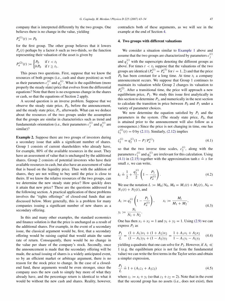
Fig. 3. The CEE discount graph.

the closed-end fund Central Europe and Russia (CEE) in 2004.In early January 2004, the net asset value and trading price wereapproximately equal. In keeping with our theory we assume thatthe liquidity price, L , was also similar. On January 9, 2004 anannouncement was made that a new rights offering would add1/3 more shares. The trading price (and the discount) beganto decline immediately. Although the actual shares would notbe issued until March 29, 2004, the “rights” were distributedto the shareholders on February 19, 2004. For every threeshares an investor held, he was given one transferable right. OnFebruary 19 these rights began trading, so that for all practicalpurposes the new shares had entered the market on this date.Fig. 3 shows the percentage discount, (P(t) − Pa(t))/Pa(t),during this period. In this example, the discount moved from0% to about 10% almost immediately after the announcement.This seems to indicate that a significant percentage of investorshad shifted their valuation to the liquidity price. When theadditional shares began trading on February 19, 2004, it waswidely anticipated, and any efficient market analysis would leadto the conclusion that it should not affect the trading price.Yet the data shows a sharp drop soon after this date. Elevendays after this date, the discount exceeded 20%, despite the factthat all of the information had been previously disseminated.This second drop is a demonstration of the importance of the“liquidity” price of an asset, a concept that is central to ourdifferential equations approach. On March 29, 2004 it appearsthat the discount narrows from about 20% to 10%. However,this is largely due to the fact that the cost and dilution effect ofthe new shares – which are known in advance – have been takenfrom the shareholders’ assets on this day. So the narrowing ofthe discount at this stage offers no benefit to the shareholders.A number of closed-end funds experienced similar events.

5. Change in number of shares

Using the example above as motivation (the actual situationhas several additional features), we consider the influx of shares

(in exchange for cash) at a particular time t2 which is notaccompanied by any announcement. We assume two groupsinitially, with Group 1 valuing the asset at Pa while Group2 values the asset at bPa (with b < 1). The total number ofshares and cash, respectively, is N0 and M0, so L0 := M0/N0.We assume that the price, P(t) = P0 is at a steady state priorto t1 and that q(i)

2 = q for both groups. Using (4.6) one cancalculate L0 if q has already been calibrated from the prior data.We assume for simplicity that L0 = Pa = P0.

Next, we suppose that at time t2, a total of N0/3 shares havebeen added to the system. We assume that Group 1 rebalancesits portfolio, but there are nevertheless N0/3 more shares in thesystem, without the addition of any new money. In other words,if US investors had, say, $200 million for investment toward thispurpose, they do not have any more after the announcement orthe issuing of new shares. Then we can write

x1 =M1

M0, y1 =

N1

4N0/3,

x2 =M2

M0, y2 =

N2

4N0/3(5.1)

and let Lnew be the new liquidity price given by the newcash/(number of shares):

Lnew =M0

4N0/3=

34

L0. (5.2)

Hence, the new liquidity value is only three-quarters of theprevious, due to the influx of new shares. We can now use (4.8)with Lnew in place of L to obtain the new equilibrium price, P1:

P1

0.75L0=

1 + 2q

1 + 2(0.75)q{1 +12 ( 1

b − 1)z2}. (5.3)

Note that for q = 1 and z2 = 0 we have from (5.3) thatP1 = 0.9L0. For q = 1, z2 = 1 and b = 0.8 (i.e., the assetsof the two groups are comparable and the second group has avaluation of 80% of the first group) we have P1 = 0.837 L0.


Fig. 4. The ratio P1/Pa as a function of the relative assets z2 for the values of q = 1 (left), and q = 1/3 (right).

Fig. 5. The price P(t) as a function of t for times t < t2 with qi2 = 0.3.

Hence, if the group that holds the cash, and is looking for abargain price, has about half of the total assets, then the pricedrops from the fundamental value to just under 84% of its value.For q = 1 and different values of z2 the ratio P1/Pa is shown inthe graph on the left in Fig. 4. For q = 1/3 we obtain the graphon the right in Fig. 4.

These calculations suggest that the influx of additionalshares in significant quantities is very likely to suppress theprice by a large amount, even if there is no change in thevaluation or the perception of value. In other words, theclosed-end fund loses up to 25% of its trading price dueto the additional influx of shares, even though both groupsperceive the valuation to be much higher. This result highlightsthe key advantage of this methodology. Methods of classicalfinance are not useful in this situation as they predict thata discount of zero percent would continue regardless of thenumber of shares issued by the management. This is due tothe concept of infinite arbitrage that indicates any discountwould be immediately eliminated as investors quickly buyup shares that were at a discount from net asset value. Ourmethodology, however, allows one to determine the discountas a function of a limited number of parameters that can be

calibrated through optimization from previous data, and fromother related situations (e.g., similar closed-end funds).

6. Numerical computations

In this section we perform numerical computations on theproblems discussed in Sections 4 and 5. Also, using thenumerical methodology we can calculate the price dynamicsthat include both of the effects: the announcement of moreshares and, later, the influx of the actual shares, and thetransition between these steady states. Hence we assume thatan announcement is made at time t1 that there will be 1/3 moreshares that are to be distributed at time t2. Prior to t1 we assume(as above) that L0 = P0 = P(i)

a =: Pa . For t1 < t < t2Group 1 continues to value the asset at Pa while Group 2 valuesit at the anticipated new liquidity price, Lnew = 3L0/4 (see(5.2) above). At time t2 the additional shares are distributed intothe system so that the new total number of shares increases to4/3N0.

In terms of initial conditions we assume that ζ1 = 0 sincethe price is assumed to be constant prior to the announcement,and ζ2 = 0 since the price is assumed to be at the fundamentalvalue. Both groups are assumed to have the same q1 and q2which we vary in the range (0,1). Also, we vary the assets ofeach group initially, ranging from Group 2 owning all of theassets to just 1/3 of the assets.

In each of the computer runs below, Eqs. (2.1), (2.2), (2.6),(2.7), (2.10) and (2.13)–(2.15) were used, and we define t1 := 9as the announcement time and t2 := 18 as the time at which thenew shares enter the market. We used the Matlab ODE packagefor these computations. The ODE package can solve problemsM(t, y) ∗ y′

= F(t, y) with mass matrix M that is nonsingular,or singular. More details can be obtained from the help menu inMatlab.

In Fig. 5, we calculate the time evolution of the price untilthe new shares are distributed into the system, i.e., P(t) iscalculated as a function of t for times t < t2. Recall thatboth groups value the asset at Pa := P(i)

a = L0 prior to theannouncement made at t = t1. Once the announcement is made,the first group continues the same valuation while the second


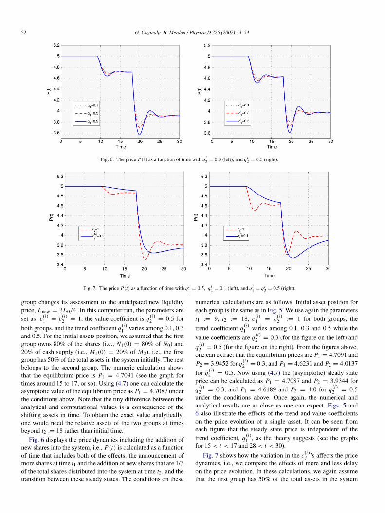
Fig. 6. The price P(t) as a function of time with qi2 = 0.3 (left), and qi

2 = 0.5 (right).

Fig. 7. The price P(t) as a function of time with qi1 = 0.5, qi

2 = 0.1 (left), and qi1 = qi

2 = 0.5 (right).

group changes its assessment to the anticipated new liquidityprice, Lnew = 3L0/4. In this computer run, the parameters areset as c(i)

1 = c(i)2 = 1, the value coefficient is q(i)

2 = 0.5 for

both groups, and the trend coefficient q(i)1 varies among 0.1, 0.3

and 0.5. For the initial assets position, we assumed that the firstgroup owns 80% of the shares (i.e., N1(0) = 80% of N0) and20% of cash supply (i.e., M1(0) = 20% of M0), i.e., the firstgroup has 50% of the total assets in the system initially. The restbelongs to the second group. The numeric calculation showsthat the equilibrium price is P1 = 4.7091 (see the graph fortimes around 15 to 17, or so). Using (4.7) one can calculate theasymptotic value of the equilibrium price as P1 = 4.7087 underthe conditions above. Note that the tiny difference between theanalytical and computational values is a consequence of theshifting assets in time. To obtain the exact value analytically,one would need the relative assets of the two groups at timesbeyond t2 := 18 rather than initial time.

Fig. 6 displays the price dynamics including the addition ofnew shares into the system, i.e., P(t) is calculated as a functionof time that includes both of the effects: the announcement ofmore shares at time t1 and the addition of new shares that are 1/3of the total shares distributed into the system at time t2, and thetransition between these steady states. The conditions on these

numerical calculations are as follows. Initial asset position foreach group is the same as in Fig. 5. We use again the parameterst1 := 9, t2 := 18, c(i)

1 = c(i)2 := 1 for both groups, the

trend coefficient q(i)1 varies among 0.1, 0.3 and 0.5 while the

value coefficients are q(i)2 = 0.3 (for the figure on the left) and

q(i)2 = 0.5 (for the figure on the right). From the figures above,

one can extract that the equilibrium prices are P1 = 4.7091 andP2 = 3.9452 for q(i)

2 = 0.3, and P1 = 4.6231 and P2 = 4.0137

for q(i)2 = 0.5. Now using (4.7) the (asymptotic) steady state

price can be calculated as P1 = 4.7087 and P2 = 3.9344 forq(i)

2 = 0.3, and P1 = 4.6189 and P2 = 4.0 for q(i)2 = 0.5

under the conditions above. Once again, the numerical andanalytical results are as close as one can expect. Figs. 5 and6 also illustrate the effects of the trend and value coefficientson the price evolution of a single asset. It can be seen fromeach figure that the steady state price is independent of thetrend coefficient, q(i)

1 , as the theory suggests (see the graphsfor 15 < t < 17 and 28 < t < 30).

Fig. 7 shows how the variation in the c(i)j ’s affects the price

dynamics, i.e., we compare the effects of more and less delayon the price evolution. In these calculations, we again assumethat the first group has 50% of the total assets in the system


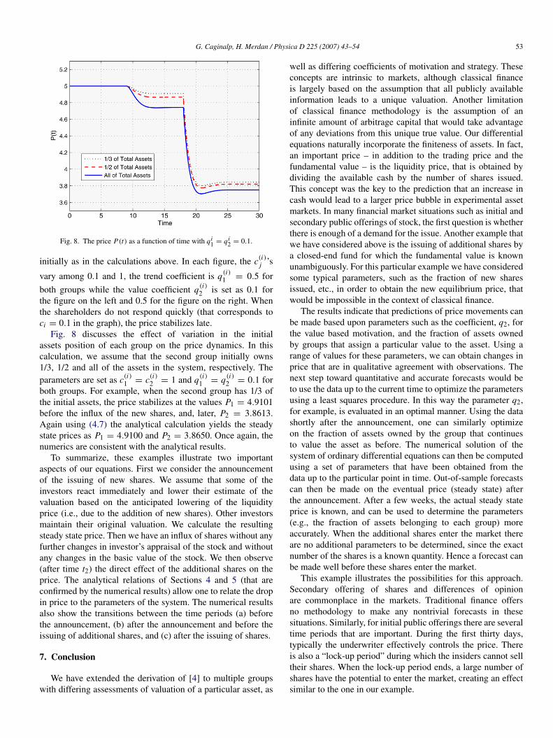
Fig. 8. The price P(t) as a function of time with qi1 = qi

2 = 0.1.

initially as in the calculations above. In each figure, the c(i)j ’s

vary among 0.1 and 1, the trend coefficient is q(i)1 = 0.5 for

both groups while the value coefficient q(i)2 is set as 0.1 for

the figure on the left and 0.5 for the figure on the right. Whenthe shareholders do not respond quickly (that corresponds toci = 0.1 in the graph), the price stabilizes late.

Fig. 8 discusses the effect of variation in the initialassets position of each group on the price dynamics. In thiscalculation, we assume that the second group initially owns1/3, 1/2 and all of the assets in the system, respectively. Theparameters are set as c(i)

1 = c(i)2 = 1 and q(i)

1 = q(i)2 = 0.1 for

both groups. For example, when the second group has 1/3 ofthe initial assets, the price stabilizes at the values P1 = 4.9101before the influx of the new shares, and, later, P2 = 3.8613.Again using (4.7) the analytical calculation yields the steadystate prices as P1 = 4.9100 and P2 = 3.8650. Once again, thenumerics are consistent with the analytical results.

To summarize, these examples illustrate two importantaspects of our equations. First we consider the announcementof the issuing of new shares. We assume that some of theinvestors react immediately and lower their estimate of thevaluation based on the anticipated lowering of the liquidityprice (i.e., due to the addition of new shares). Other investorsmaintain their original valuation. We calculate the resultingsteady state price. Then we have an influx of shares without anyfurther changes in investor’s appraisal of the stock and withoutany changes in the basic value of the stock. We then observe(after time t2) the direct effect of the additional shares on theprice. The analytical relations of Sections 4 and 5 (that areconfirmed by the numerical results) allow one to relate the dropin price to the parameters of the system. The numerical resultsalso show the transitions between the time periods (a) beforethe announcement, (b) after the announcement and before theissuing of additional shares, and (c) after the issuing of shares.

7. Conclusion

We have extended the derivation of [4] to multiple groupswith differing assessments of valuation of a particular asset, as

well as differing coefficients of motivation and strategy. Theseconcepts are intrinsic to markets, although classical financeis largely based on the assumption that all publicly availableinformation leads to a unique valuation. Another limitationof classical finance methodology is the assumption of aninfinite amount of arbitrage capital that would take advantageof any deviations from this unique true value. Our differentialequations naturally incorporate the finiteness of assets. In fact,an important price – in addition to the trading price and thefundamental value – is the liquidity price, that is obtained bydividing the available cash by the number of shares issued.This concept was the key to the prediction that an increase incash would lead to a larger price bubble in experimental assetmarkets. In many financial market situations such as initial andsecondary public offerings of stock, the first question is whetherthere is enough of a demand for the issue. Another example thatwe have considered above is the issuing of additional shares bya closed-end fund for which the fundamental value is knownunambiguously. For this particular example we have consideredsome typical parameters, such as the fraction of new sharesissued, etc., in order to obtain the new equilibrium price, thatwould be impossible in the context of classical finance.

The results indicate that predictions of price movements canbe made based upon parameters such as the coefficient, q2, forthe value based motivation, and the fraction of assets ownedby groups that assign a particular value to the asset. Using arange of values for these parameters, we can obtain changes inprice that are in qualitative agreement with observations. Thenext step toward quantitative and accurate forecasts would beto use the data up to the current time to optimize the parametersusing a least squares procedure. In this way the parameter q2,for example, is evaluated in an optimal manner. Using the datashortly after the announcement, one can similarly optimizeon the fraction of assets owned by the group that continuesto value the asset as before. The numerical solution of thesystem of ordinary differential equations can then be computedusing a set of parameters that have been obtained from thedata up to the particular point in time. Out-of-sample forecastscan then be made on the eventual price (steady state) afterthe announcement. After a few weeks, the actual steady stateprice is known, and can be used to determine the parameters(e.g., the fraction of assets belonging to each group) moreaccurately. When the additional shares enter the market thereare no additional parameters to be determined, since the exactnumber of the shares is a known quantity. Hence a forecast canbe made well before these shares enter the market.

This example illustrates the possibilities for this approach.Secondary offering of shares and differences of opinionare commonplace in the markets. Traditional finance offersno methodology to make any nontrivial forecasts in thesesituations. Similarly, for initial public offerings there are severaltime periods that are important. During the first thirty days,typically the underwriter effectively controls the price. Thereis also a “lock-up period” during which the insiders cannot selltheir shares. When the lock-up period ends, a large number ofshares have the potential to enter the market, creating an effectsimilar to the one in our example.


Even in the absence of additional shares, there is often theissue of different groups having very different views on thevalue of an asset. In some cases the differences in valuationare extreme. For example in the internet/high-tech bubble,there were shares trading for $200 that fundamental investorsvalued at $5. Since investors buying at $200 were oftenmomentum players, falling prices usually induced selling ratherthan buying. But with the value investors not interested untilthe price fell to a few percent of the former levels, the declinebecame a free fall. Thus, the approach we develop has thepotential to address quantitatively the issues that are trivializedin classical economics and finance.

Acknowledgement

This research was supported by LGT Asset Management.The authors may have long or short positions on securitiesdiscussed in the paper.

References

[1] T. Beard, B. Beil, Do people rely on the self-interested maximization ofothers? An experimental test, Manag. Sci. 40 (1994) 252–262.

[2] D. Davis, C. Holt, Experimental Economics, Princeton University Press,Princeton, NJ, 1993.

[3] G. Caginalp, G.B. Ermentrout, A kinetic thermodynamics approach to thepsychology of fluctuations in financial markets, Appl. Math. Lett. 4 (1990)17–19.

[4] G. Caginalp, D. Balenovich, Asset flow and momentum: Deterministicand stochastic equations, Philos. Trans. R. Soc. Lond. Ser. A 357 (1999)2119–2133.

[5] G. Caginalp, D. Balenovich, Market oscillations induced by thecompetition between value-based and trend-based investment strategies,Appl. Math. Financ. 1 (1994) 129–164.

[6] D. Fudenberg, J. Tirole, Game Theory, MIT Press, Cambridge, MA, 1993.[7] D. Kahneman, A. Tversky, Prospect theory: An analysis of decision making

under risk, Econometrica 47 (1979) 263–291.[8] L. Lopes, Between hope and fear: The psychology of risk, Adv. Exp. Soc.

Psychol. 20 (1987) 255–295.[9] H. Shefrin, A Behavioral Approach to Asset Pricing, Elsevier, 2005.

Documents

Asset price dynamics with heterogeneous groups