Embed Size (px)
Citation preview

Copyright © 2002, by the author(s). All rights reserved.
Permission to make digital or hard copies of all or part of this work for personal or
classroom use is granted without fee provided that copies are not made or distributed for profit or commercial advantage and that copies bear this notice and the full citation
on the first page. To copy otherwise, to republish, to post on servers or to redistribute to lists, requires prior specific permission.

COULOMB INTERACTIONS
IN HIGH THROUGHPUT
ELECTRON BEAM LITHOGRAPHY
by
Bo Wu
Memorandum No. UCB/ERL M02/4
26 February 2002
COULOMB INTERACTIONS
IN HIGH THROUGHPUT
ELECTRON BEAM LITHOGRAPHY
by
BoWu
Memorandum No. UCB/ERL M02/4
26 February 2002
ELECTRONICS RESEARCH LABORATORY
College ofEngineeringUniversity ofCalifornia, Berkeley
94720
Coulomb Interactions in High Throughput Electron Beam Lithography
by
BoWu
B.A. (University ofRochester) 1992M.S. (University ofMichigan, Ann Arbor) 1994
A dissertation submitted in partial satisfaction ofthe
requirements for the degree of
Doctor ofPhilosophyin
Physics
in the
GRADUATE DIVISION
ofthe
University ofCalifornia at Berkeley
Committee in charge
Professor Andrew R. Neureuther, ChairProfessor Jonathan Wurtele, Cochair
Professor W. Oldham
Professor Roger Felcone
Spring 2002

The dissertation ofBo Wu is approved:
Chair Date
Cochair Date
Date
Date
University ofCalifornia, Berkeley
Spring 2002
Coulomb Interactions in High ThroughputElectron Beam Lithography
Copyright 2002
by
Bo Wu

Abstract
Coulomb Interactions in High Throughput Electron Beam Lithography
by
BoWu
Doctor ofPhilosophy in Physics
University ofCalifornia at Berkeley
Professor Andrew R. Neureuther, Chair
Professor Jonathan Wurtele, Cochair
High throughput electron beam lithography systems have been viewed as
promising candidates for sub-lOOnm wafer writing tools. This thesis extends previous
work in the study of electron Coulomb interactions and the study of electron interactions
with photo-resists. Both of these interactions contribute to image blur and the studies in
this thesis provide physical insight, quantitative characterization and suggestmethods of
reducing blur.
The Berkeley Electron Beam Simulator (BEBS) is a collection of software tools
developed by the author to study the charged particle interactions in beam columns.
BEBS employs the Fast Multi-pole Method (FMM) for rigorous force calculations. It
takes about one hour with ten 500MHzprocessors to simulate a 30pA beam current in a.
typical 4x demagnification system usinga packetof 13,000 particles. The accuracy ofthe
force calculation algorithm is benchmarked with that ofMunro's electron beam simulator.
BEBS provides many optionsfor observing forces and trajectorychanges, and improving
beam spot size. These options have been successfully applied and proved especially
useful in studying stochastic interactions affecting beam blur.
The influence of space charge on the electron dynamics is investigated with
simulations.The primary consequenceof space charge is beam blur. Beam blur reduction
techniques are examined using both neutralizing ions and lens aberrations. Results show
that around 80% of the space charge blur is eliminated at 30pA beam current and that the
total beam blur is reduced by nearly 30%. Further beam blur reduction would be
formidable unless the stochastic blur is also reduced.
The basic assumptions of Mkrtchyan's Nearest Neighbor Theory are tested. It is
demonstrated that for typical e-beam lithography applications, electron interaction with
multiple neighbors rather than the nearest neighbors is the norm other than exception in a
typical electron beam system. The simulation shows that the randomized correlation
length is a fimction of the beam diameter and that correlated interactions occur at other
axial positions due to symmetry with respect to the beam crossover. The structures of
stochastic Coulomb interactions have been analyzed in probe-forming systems through a
novel approach that combines algebraic analysis of forces and simulation of relocated
trajectory displacements. This approach is able to explain why a crossover beam and a
homocentric parallel beam with the same beam angle produce the same beam blur in spite
ofthe high electron densities that occur in the crossover case.
Scaling laws for stochastic blur are developed. In a beam projection or multi^
emitter array system, the stochastic blur is proportional to beam current raised to the
power of 0.62, which roughly agrees with Jansen's prediction of 0.67. The scaling laws
of the stochastic blur are also formulated with respect to column length, beam
convergence angle, emitter spacing and beam voltage.

Professor Andrew R. Neureuther
Dissertation Committee Chair
Professor Jonathan Wurtele
Dissertation Committee Cochair
Table ofContents
CHAPTER 1. Introduction 1
1.0 Tools 11.1 Thesis 2
1.2 Academic contributions 4
CHAPTER 2. Background 8
2.0 Challenges 82.1 Stochastic effect 9
2.2 Space charge effect 102.3 Simulation tools 11
2.4 Electron-resist interactions 13
CHAPTER 3. Beam Electron Beam Simulator - algorithms and characteristics15
3.0 Introduction 15
3.1 Force computations in BEBS 153.1.0 Pbody library 153.1.1 Electron bunch 17
3.1.2 Lorentz transformations 18
3.2 Time iteration 20
3.3 Post-processing ofdata 233.4 Special options in BEBS 253.5 Comparison with Munro's Software 273.5.1 Barnes-Hut algorithm 273.5.2 Accuracy and speed comparison 28
CHAPTER 4. Beam Blur Contributions in Multi-emitter Array Systems 34
4.0 Introduction 34
4.1 Blur contribution along the optical axis 344.2 Inter-beamlet, intra-beamlet electron interactions and the
summation rule 39
4.2.0 Mask configurations 394.2.1 Summation rule for beam blur contributions , 404.2.2 Inter-beamlet and intra-beamlet blur contributions 41
4.2.3 Inter-beamlet blur contribution and emitter spacing on the mask 434.3 Conclusions 46
CHAPTER 5. Stochastic Coulomb Interactions and Neighboring Electrons 47
5.0 Introduction 47
5.1 System setup 47
5.2 Numbers ofneighboring electrons 495.3 Effect ofneighboring electrons upon the transverse forces 525.4 Conclusions 55
CHAPTER 6. Structure Of Stochastic Coulomb Interactions 56
6.0 Introduction 566.1 Stochastic interactions in a probe-forming beam with a crossover 586.1.0 Stochastic force upon a single electron 586.1.1 Averaged stochastic force 606.1.2 Blur contribution along the optical axis 646.2 Stochastic interactions in a homocentric parallel beam 696.3 Other probe forming beam configurations 726.4 Stochasticinteractionsin a systemwith multi-emitterarray 736.5 Conclusions 75
CHAPTER 7. Scaling Laws for Stochastic Coulomb Interactions 76
7.0 Introduction 767.1 Theory 787.2 Scaling laws 807.2.0 Comparison with Jansen's Theory 807.2.1 Scaling laws for a 25-emitter array system 81
CHAPTER 8. Impact of Positive Ions and Effect of Lens Aberrations 86
8.0 Introduction 868.1 Impact ofpositive ions 878.2 Effect of lens aberrations 928.3 Summary and conclusions 95
CHAPTER 9. Electron Interaction with Photo-resist 96
9.0 • Introduction 96
9.1 Schematics ofERIM 979.2 Secondary electron emission process 999.3 Exposure process 1029.4 Spatial profile ofexposure events 1059.5 Exposure dose 1069.6 Conclusions and discussion 107
CHAPTER 10. Conclusions 110
10.0 Numerical and analytical tools 11010.1 Mechanism studies and beam blur reductions Ill
10.2 Future work 114
Bibliography 117
11
Acknowledgements
I would like to thank my advisor, Professor Andrew R. Neureuther for helping me
make this transition to application oriented research. Without his guidance and support, I
would not have been able to complete my thesis project within three years. He is a role
model for me with his enthusiasm, diligence, and uncompromising standards.
I would like to thank my physics co-advisor. Professor Jonathan Wurtele, for his
consistent support. His insight and outlook as a physicist makes my thesis a physics one.
Thanks are due to Professor Roger Falcone, former Chair of the physics department, for
his understanding and steady support. I would also like to thank Professor William
Oldham for serving on my qualifying and thesis committees. I am gratefiil to Professor
Wulf Kunkel for serving on my qualifying committee.
I had the good fortune of working with my colleagues and friends. Dr. Mosong
Cheng, Dr. Ebo Croffie, Lei Yuan, Michael Williamson, Yunfei Deng, Yashesh Shroff,
Mr. Junwei Bao, Yijian Chen, Jason Cain, Garth Robins, Dr. Liqun Han and Dr. Gil
Vinograd for their friendship to support. Mosong and Ebo were especially helpful during
the initial stage of this research project. They helped me more than they probably ever
realized.
Ill
I would like to thank my immediate and extended families for their support
throughout my education. Last but not least, I thank the Lord for answering my prayers
and for helping me all the way through this incredible journey.
IV

1 Introduction
High throughput electron beam systems, such as SCALPEL [1] and PREVEAIL
[2], have been used as potential candidates for sub-lOOnm lithographic tools. The
ultimate resolution in high throughput electron beam lithography is strongly limited by
the electron-electron interactions in the beam column [3] [4] and the electron interactions
with photo-resist [5]. A thorough understandingof these interactions is vital to the design
ofany high throughput electron beam systems.
1.0. Thesis
The contents of this thesis are classified into two categories: (a) analytical and
simulation tools, including the characteristics of the Berkeley Electron Beam Simulator
(BEBS) developed by this author and its algorithms, and (b) scientific contributions in the
study of electron interactions in beam columns and the study of electron interaction with
photo-resist. This chapter highlights the thesis contribution and provides a few key
references. The general background is provided in Chapter 2 with more complete
references.

1.1. Tools
Experimenting with high throughput electron beam systems is very costly and
timeconsuming. System modeling gives insight to the physical mechanisms and provides
general guidelines for the design. A large number of theoretical works have been
dedicated to the study of the electron stochastic interactions [6] [7] and the global space
charge effect [3] in electron beam columns. Among these, simulation techniques provide
a powerful tool for the study of the collective behavior of a large number of charged
particles in the beamcolumn. All the beamand column parameters canbe easily tuned in
simulations. The simulation approach is particularly useful in the study of the electron
stochastic blurs when the analytical approach is formidable.
A serious drawback of some existing electron beam simulators is that the
computation time is proportional to the square of number of electrons, which makes the
highbeam current simulation intractable. Munro et al. have been developing conunercial
software for the design of electron beam lithographic systems [8] [9]. Since the initiation
of this thesis work, Munro uses the Bames-Hut method [10] in his commercial electron
beam simulator to reduce the amount of computation required [11]. A detailed
comparison between BEBS and Munro's simulator is provided in Section 3.6 of this
thesis. Han and Winograd [12] [13] developed an electron beam simulator at Stanford
University to study the global space charge effect. Its force computations, however, are
based on an unverified approximation of"test" electrons and "field" electrons.
The force computations in the BEBS are performed with Pbody [14] [15], which
is a parallel libraryrunning on multiple processors. It employs the Fast MultipoleMethod
(FMM) [16] [17] for fast and rigorous force calculations. The computation time is
roughly proportional to the number of electrons and inversely proportional to the number
ofprocessors.
Compared with other existing electron beam simulators, BEBS provides a number
of special options for the study of beam blur production mechanisms. These options
include identifying the neighboring electrons of an arbitrary electron of concern, directly
generating stochastic blurs in simulations through the use of positrons, etc. Each option
has been successfully applied in the academic contributions of this thesis. Chapter 3 will
discuss the details ofBEBS' computational algorithms and special options.
Facing many body problems, analytical approaches often lead to algebraic
expressions that are not solvable. Simulation techniques avoid this problem. Yet, the
imderl}dng physical principles may be hidden. To address these shortcomings, the author
developed an approach [18] which combines analytical approach and simulation
technique and uses the strength of both. This new approach is successftilly applied to the
study of the structure ofelectron stochastic interactions in Chapter 6.
Some early work on electron-resist interactions owes to Greeneich [19] [20] and
Shimizu [21] on the modeling of electron-resist interaction. In 1980's Murata et al [22]
[23] developed the hybrid model to study energy deposition in photo-resist. Murata's

model, however, is based onthe assumption that ail forms ofdeposited energy contribute
equally to the exposure events and the detailed mechanisms of exposure reactions were
not considered.
The Electron-Resist Interaction Model (BRIM) presented in Chapter 9 of this
thesis is the first of its kind to study the electron resist interaction mechanisms using
reaction cross sections [24]. BRIM is a pure analytical model, which gives an algebraic
expression for the spatial distribution ofexposure events.
1.2. Academic contributions
This thesis first examines the beam blur contributions in terms of axialpositions,
and inter- and intra-beamlet electron interactions [25]. The results are presented in
Chapter 4. The chapter also presents the summation rule of inter- and intra-beamlet
interactions.
The electron statistical interactions create image blurs that are not correctable
through conventionaloptical system compensation. Theoristsdeveloped differentmodels
to predict the beam blur caused by the electron-electron stochastic interactions in various
beam configurations. Mkrtchyan [6] formulated an analytical model based on the nearest-
neighbor approximation. Jansen [7] [26] developed the Extended Two-Particle model for
high throughput electron beam systems. Both model also require a series of
approximations and untested assumptions.

In Chapter 5 of this thesis, the nearest-neighbor assumption of Mkrtchyan's is
tested via simulations. Analysis of a basic crossover showed that interactions with
multiple rather than nearest-neighbor electrons almost immediately became the nonn
rather than the exception.
Jansen's Extended Two-Particle model predicts that a crossover beam and a
homocentric parallel beam can produce the same beam blur as long as they share the
same beam angle [27]. However, the physical insight is completely buried in the
mathematical complexity ofhis analysis.
Chapter 6 of this thesis provides physical insight and quantitative explanation of
Jansen's above prediction. The chapter reveals the rich structures of stochastic
interactions in different beam geometries [18], which can be further explored for possible
beam blur reduction.
Chapter 7 presents a stochastic effect simulator, which is the first of its kind to
produce stochastic blur directly in simulation. It is effectively used to develop the scaling
laws for the stochastic blur and the scaling laws for the space charge blur. The chapter
also provides the theoretical foundation for the stochastic effect simulator.
Han and Winograd [3] [12] demonstrated that the aberrations induced by the
lensing action of global space charge of the electrons result in beam blur that increases
with beam current. The space charge effect seriously limits the performance of high

throughput electron beam lithography systems. It was demonstrated in experiments that
the spherical aberrations of a focused ion beam can becorrected via electron clouds [28]
[29]. However, it was not clear whether the neutralization scheme would be applicable
for a high throughput e-beam lithography system due to the scattering of small-mass
electrons. Xiu [30] [31] studied the effect ofspace charge coils and a multi-pole projector
in electron beam columns and tried to reduce field curvature and on-axis aberrations.
Nevertheless, no quantitative results have been given on beam blur reductions.
Chapter 8 of this thesis discusses the impactofpositive ions in beam columns and
the effect of lens aberrations as potential techniques to reduce space charge blurs. Results
demonstrate that total beam blur can be considerably reduced with either technique in
high throughput electron beam systems [32].
The hybrid model developed by Murata [22] is a Monte Carlo program used to
simulate the exposure profile of e-beam resist. This model, however, is based on the
assumption that all forms of deposited energy contribute equally to the exposure events,
which hasno physical basis. Theexposure mechanisms are beyond the scope of Murata's
model.
Chapter 9 of this thesis examines the mechanisms.of electron-resist interactions.
The chapter reveals the parameter dependencies of the miniTnnm exposure dose and the
roles of secondary electrons with the ERIM model [24]. The author derives an analytical
expression for the spatial distribution of exposure events, which is suitable for numerical
solution.

2 Background
High throughput electron beam lithography systems are viewed as promising
candidates for the next generation of wafer writing tools. In contrast to optical
lithography, the resolution of electron beam lithography is no longer limited by
wavelength. Several different types of high throughput electron beam systems have been
proposed or developed with the goal of producing sub-lOOnm wafer-writing tools. In a
projectionelectron beam system, such as SCALPEL [1] and PREVAIL [2], developed by
Lucent and IBM, respectively, the mask is flood-illuminated by a beam of electrons, and
the image is projected on the surface of the wafer. In a multiple emitter array system,
each individual emitter can be tuned on or off and patterns on the emitter array are
projected onto the wafer.
2.0. Challenges
The disadvantage of electron beam lithography is that the demands for high
resolution and high throughput are contradictory due to the repelling forces between
electrons in the beam column [33] [34]. Meanwhile, the interaction of an electron beam
with photo-resist films produces a spatial distribution of exposure reactions, which
imposes another limitation to the resolution of electron beam lithography [35] [36].
8
Numerous efforts have been made to reduce beam blur at high beam currents to meet a
given resolution and throughput requirement.
2.1. Stochastic effect
The electron statistical interactions create image blur that is not correctable
through conventional optical system compensation. Different theoretical models have
been developed to predict the beam blur caused by the electron-electron stochastic
interactions. Berger et al tried to investigate the trajectory displacement effects using
Monte Carlo methods [33]. However, the stochastic effect is always convoluted with the
spacechargeeffect in his studies. The stochasticeffect was never isolated. Weidenhausen
et al first introduced the nearest-neighbor (N-N) approach to study the electron
stochastic effect in probe-forming systems [37] [38]. Based on the N-N approach,
Mkrtchyan et al developed a new model to examine the stochastic interactions in high
throughput e-beam systems [6] [39]. Both models are based on consideration of the
nearest-neighbor electrons and on the concept of a randomized length, over which
interactions are correlated. Mkrtchyan was then able to get agreement with the limited
experimental data for a wide range of beam currents. Meanwhile, Van Leeuwen and
Jansen proposed the Multiple Independent Collision Approach (MICA) for probe-
forming systems [40]. To isolate the stochastic effects the model only considers the
collisions of the electrons on the trajectory that runs through the center of a circular
beam. Jansen refined the above approach and developed the extended two-particle model
for projection e-beam systems [7]. Jansen's model still requires either a first order
approximation or a strong- single-collision approximation. Jansen predicts that a

crossover beam and a homocentric parallel beam produce the same beam blur as longas
they share the same beam angle [27]. This prediction was later confirmed in simulation
results by Brodie et al [41] and Han [42]. Nevertheless, the sophisticated mathematical
formulation of his model failed to give convincing physical insight into this problemand
the structure of electron stochastic interactions remains hidden.
2.2. Space charge effect
The aberrations induced by the lensing action of global space charge of the
electrons also result in beam blur that increases with beam current. Han and Winograd
[3][12] have demonstrated through simulations that the allowable current in a high
throughput electron beam projection system is strongly limited by these aberrations. In
particular, beam-induced space curvature and astigmatism have been recognized as the
major contributors to the beam blur. The space charge effect was later observed and
studied in the SCAPEL system [43] [44].
Techniques that effectively reduce the space charge effect are vital to the
realization of high throughput electron beam lithography tools. The space charge
neutralization of electron beams using positive ions has been investigated since 1920's
when cathode ray tube was a main focus of the study [45] [46]. In the mid 20*** century,
topics which involved neutralization were beam transport phenomena, plasma physics
and elementary particle physics. The space charge neutralization of ion beams using
electrons was demonstrated [47]. In 1997 Chao [28] et al and Orloff [29] show that the
10
spherical aberrations in ion beams can be corrected via electron clouds. However, it was
not clear whether the neutralizationscheme would be applicable for a high throughput e-
beam system due to the scattering of electrons. Xiu [30] [31] later studiedthe impact of
space charge coils and a multi-pole projector in electron beam systems trying to reduce
the field curvature the other space charge induced aberrations in the SCALPEL system.
Nevertheless, no quantitativeresults havebeen givenon beamblur reductions.
2.3. Simulation tool
Simulationtechniques serveas a powerful tool for the studyof electron Coulomb
interactions in the beam column. It is particularly usefiil in the study of the electron
stochastic blur when the analytical approach is formidable. In comparison with
experimental techniques, all the beam and column parameters can be easily tuned in
simulations.
The largest computational obstacle in the simulation of electron beams is the
calculation of the forces exerted on each electron by the other electrons. Calculating this
directly is prohibitively time consuming as the computation time grows as the square of
the number of particles. A great deal of literature has been devoted to the study of
reducing the amount of computation time by allowing the use of approximations. For
calculations where high accuracy is not essential, the method of Bames and Hut [10] is a
possible choice, which is used in Munro's commercial electron beam simulation software
[11]. The amount of work required by the Bames-Hut method to perform the force
calculation for N particles is proportional to AHogA^.
11
Jansen developed the Fast Monte Carlo Simulation (FMCS), which combine the
Monte Carlo approach with his Extended Two-particle theory [48]. The accuracy of the
simulation, however, is limited by the unverified assumptions and approximations in
Jansen's theory. Moreover, the detailed mechanisms of electron-electron interactions can
no longer be examined due to these approximations.
The Stanford electron beam simulator, uses "field electrons" and "test electrons"
to avoid the large amount of calculations [12] [13]. In this model, all the field electrons
follow completely straight trajectories and only provide background electric field for the
test electrons. This approximation tends to overestimate the effect of Coulomb
interactions in the column. The simulator was mainly used for the study of global space
charge effect in beam projection systems.
For simulations that require more accuracy, the Fast Multipole Method (FMM) of
Greegard, Carrier and Rokhin [16] is an appropriate choice. Here the amount of work
required to perform the calculation is proportional to the number of particles. For a high
level of accuracy, it is more efficient than the Bames-Hut algorithm. Carmichael [49] and
Wen at al [50] employs a fidly rigorous Fast Multipole Method (FMM) using the
DPMTA code firom Duke [51] to perform the force calculations, for his electron beam
simulator. Wen's implementation of FMM does not include local refinement in spatial
divisions, which limits its efficiency for highly non-uniform electron distributions, such
as a crossover beam.
12

2.4. Electron-resist interactions
In 1968Reimerpublished the single scattering Monte Carlo model [52], in which
electron scatterings in solids are simplified by separating the effects of elastic and
inelastic scattering events. The angular deflection of an electron is determined by the
elastic scattering based on the Rutherford cross section and the energy loss between
scatterings is calculated by the continuous slowing down approximation of the Bethe law
[53]. The single scattering model has been refined by Reimer et al [54], Curgenven and
Duncumb [55], Murata el al [56]. Based on these past studies the Monte Carlo
simulation with single scattering was applied to fundamentals of electron beam
lithography. The reports by Shimizu and Everhart [21] and Shimizu et al [57] were
concerned with energy deposition in bulk PMMA targets. Nevertheless, the single
scattering model does not include inelastic collisions or secondary electron productions,
which cause spreading ofenergy absorption.
Based on the single scattering model, Murata et al [22] [58] later developed a
hybrid model for lithography applications, which includes discrete energy processes and
fast secondary electron productions. The hybrid model provides the profile for the
electron energy deposited in the photo-resists. Vriens cross section [59] and the modified
Bethe formula by Joy and Luo [60] were used to describe the discrete energy processes.
Both models, however, are based on the assumption that all forms of deposited energy
contribute equally to the exposure events, which has no physical basis. The detailed
mechanisms of exposure reactions are beyond the scope of these models.
13
In 1992 Lutwyche [61] proposed a semi-classical model to study the resolution of
e-beam lithography. G. Han and F. Cerrina [62] later developed an analytical model
based on the theory of \drtual quanta. In these models, all the exposure events were
attributed to the high energy primary electrons. The impact of secondary electrons was
not included in the discussions. Moreover, they use overly simplified models for the
resist molecules, which overlooks most ofthe exposure mechanisms
14
3 Berkeley Electron Beam Simulator -
Algorithms and Characteristics
3.0. Introduction
The Berkeley Electron Beam Simulator (BEBS) is a collection of software tools
developed by the author to study the electron Coulomb interactions in beam columns.
This chapter discusses the force computations in BEBS in section 3.1. The time iteration
algorithm is presented in Section 3.2. Section 3.3 addresses the issue of post-processing
of data. Section 3.4 presents BEBS' special options for mechanism studies. Section 3.5
gives a comparison is given between BEBS and Munro's simulation software.
3.1. Force computations in BEBS
3.1.0. Pbody library
The force computations in BEBSare perfonnedwith the Pbodylibrary, which is a
parallel adaptive N-body solver developed by Blackston and Demmel [14] [15]. Pbody
employs a novel locally refinable Fast Multipole Method (FMM) [16] to achieve high
efficiency and accuracy. FMM reduces the amount of computation by using spherical
harmonics to approximate the effects of sets of particles rather than resorting to direct
calculation. The computation time is roughly proportional to the number of charge
15
particles, and inversely proportional to the number of processors, which is usually
between two to fifteen. Currently Pbodyis available on two clusters: the NOW(Network
ofWorkstations) [63] and the Millennium [64] both at UC Berkeley.
Theperformance of Pbody depends on the settings of four parameters: expansion
size P, MAXBN, SEPARATION, and the use ofsupemodes [65]. Pbody includes up to S***
order terms in its spherical harmonics expansions, namely P-5. To improve the
efficiency of the code, Pbody uses an adaptive apprpach where the regions that are
populated more densely by particles are subdivided more finely cells. Figure 3-1 is a
schematic diagram for cell divisions with at most two particles in each cell. In e-beam
applications, typically, each cell holds up to MAXBN=50 particles. A large MAXBN
results in higher accuracy at the expense of run time. Pbody directly calculates the
Coulomb forces for each pair of electrons that belong to the same cell or adjacent cells.
These direct calculations become particularly important when the neighboring particles
are from different cells [66].SEPARATION is a parameter defined in Pbody to extend the
direct calculation zone beyond adjacent cells [67] to produce a more accurate result.
SEPARATI0N=2 is chosen for BEBS. Pbody allows the use of supemodes, first
described by Zhao [68] to reduce the amount of computation with only a small cost in
accuracy. A typical 30pA current simulation (-13,000 particles) in a 40cm long colunm
takes about one hour with ten 500MHz processors. Please refer to reference [15] for a
more detailed discussion of the Pbody library. A background introduction to FMM used
in the simulation ofe-beam can be found in Chapter 2.
16

(a) Adaptive (b) Non-Adaptive
Figure 3-1. The adaptive and the non-adaptive Division of space in FMM.
3.1.1. Electron bunch
Instead offilling the entire simulation column with electrons, BEBS uses single or
multiple electron bimches to reduce the computation time. Each electron bunch is 12mm
long. In order to avoid the 'tail" effect, only the 4mm part in the middle is used to
produce image on the target plane as shown Figure 3-2. This method is discussed in
reference [13] [69] and is used both by Munro's simulation software and by the Stanford
simulator. The projection lenses, whose focal lengths are independent of electron energy,
provide a means of directly observing beam blur due to electron-electron Coulomb
interactions. These achromatic imaging lenses are appropriate for investigating effects in
electron beam lithography systems where the space charge effect and the stochastic effect
are expected to dominate image quality such as in SCALPEL.
17
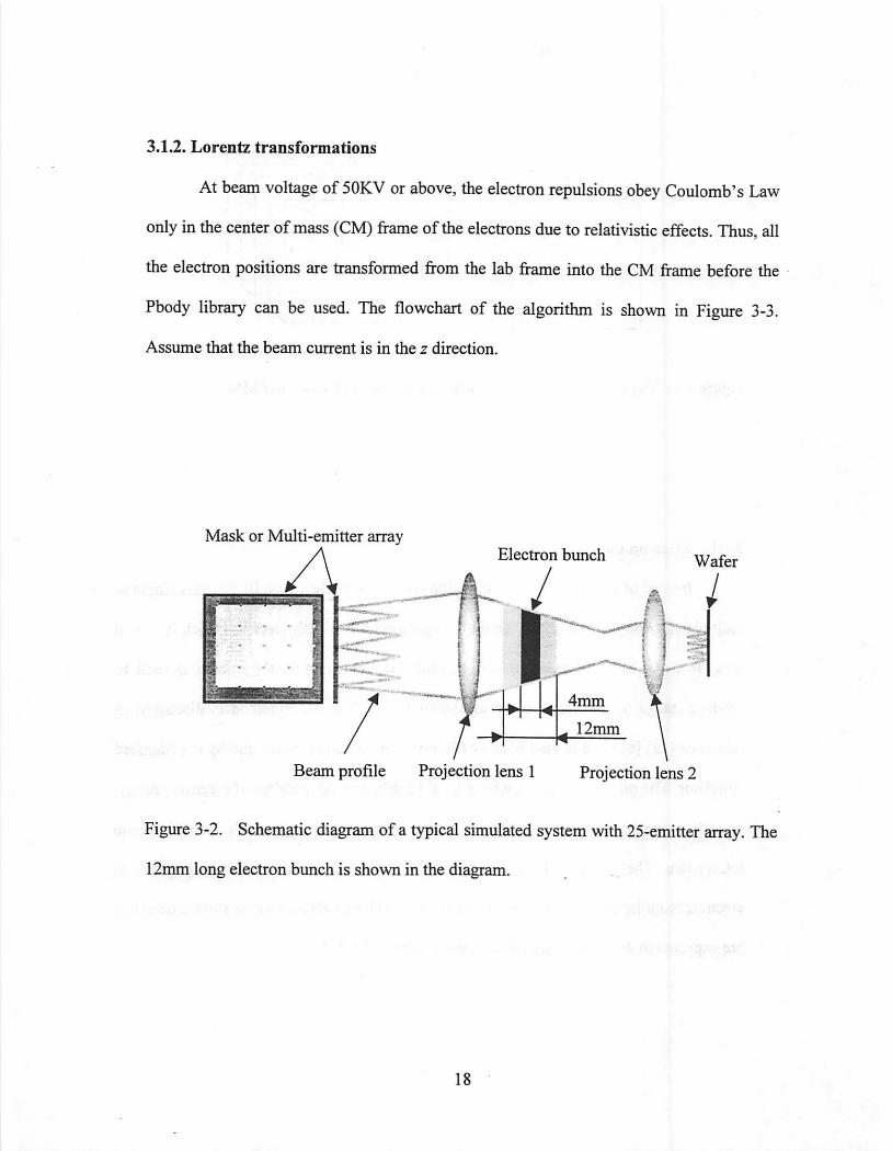
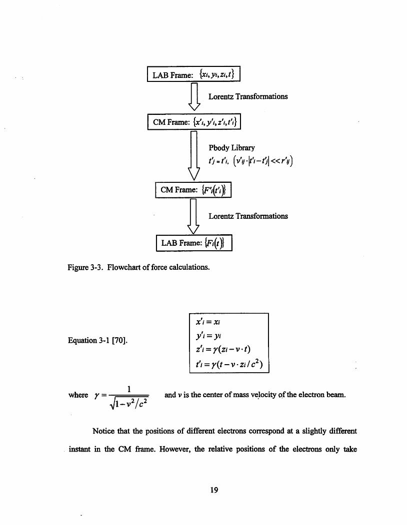
3.1.2. Lorentz transformations
At beam voltage of 50KV or above, the electron repulsions obey Coulomb's Law
only in the center of mass (CM) frame of theelectrons dueto relativistic effects. Thus, all
the electron positions are transformed from the lab frame into the CM frame before the
Pbody library can be used. The flowchart of the algorithm is shown in Figure 3-3.
Assume that the beam current is in the z direction.
Mask or Multi-emitter array
AElectron bunch
4mm
. 12mm
Wafer
Beamprofile Projection lens 1 Projection lens 2
Figure 3-2. Schematic diagram of a typical simulated system with 25-emitter array. The
12mm long electron bunch is shown in the diagram.
LAB Frame: yhzi, t}
Lorentz Transformations
V
CM Frame: {x'/, y't, z'i, t'l]
V
Pbody Library
t'j «t'i, ^vV •|/'| — « r'ijj
CM Frame:
Lorentz Transformations
LAB Frame: {F/(r)!
Figure 3-3. Flowchart of force calculations.
Equation 3-1 [70].
where y =
X i = Xi
yi = yi
z'i = y{zi-V't)
t'i = y{t-V'Zi/ c^)
and Vis the center ofmass velocity ofthe electron beam.
Notice that the positions of different electrons correspond at a slightly different
instant in the CM frame. However, the relative positions of the electrons only take
19

negligible changes withinthesetimedifferences, as indicated by Equation3-2. Therefore,
simultaneousness is a good approximation in calculating forces. The forces are
transformed back to the LAB frame before Pbody is called.
Equation 3-2 [71].Fxi= F'xi/ y
Fyi= F'yi/ y
Fzi = F'zi
3.2. Time iteration
BEES updates the positions of the electrons through a special iteration algorithm
of its own. There are two distinguished features of BEB's time iteration algorithm. First,
it uses the time steps adaptively to reduce the amount of computations needed. Second,
BEBS uses continuouslyinterpolated forces to calculateending positions.
Figure 3-4 shows the flowchart of time iteration. BEBS uses a trial time step /df
based on the result of the last time step. This sectiononly discusses movements along the
Xdirection. The movements alongy and z are treated in the same way. As an example, the
solid curve in Figure 3-4 shows the real trajectory of an electron i from t to At. The force
Fxi(t) experienced by this electron varies with time. BEBS approximates Fxift) with Fxi(t),
which would be experienced by this electron if there were no Coulomb forces and all the
electrons in the colunm traveled along straight lines, as shown in Figure 3-4. Fxi(t) is
further approximated with parabolic function Fxi(T) »Axi(T't)^+Bxi(T-t)+Cxi9 where the
coefficients Axh Bxi and Cxi are solutions from the relations given by Equation 3-3.
20

Equation 3-3.
Therefore,
Equation 3-4.
C,i=Fxi{t)
Axi(At/2) ^+Bxi(At/2)+Cxi— Fxi(jt+A/ /2)
Axi(At) ^+Bxi(At)+Cxi- Fxi{t +At)
Fxi(T) WFxi(r) « Axi(T'tf+Bxi(T-t)+Cxi, t<T<t +At
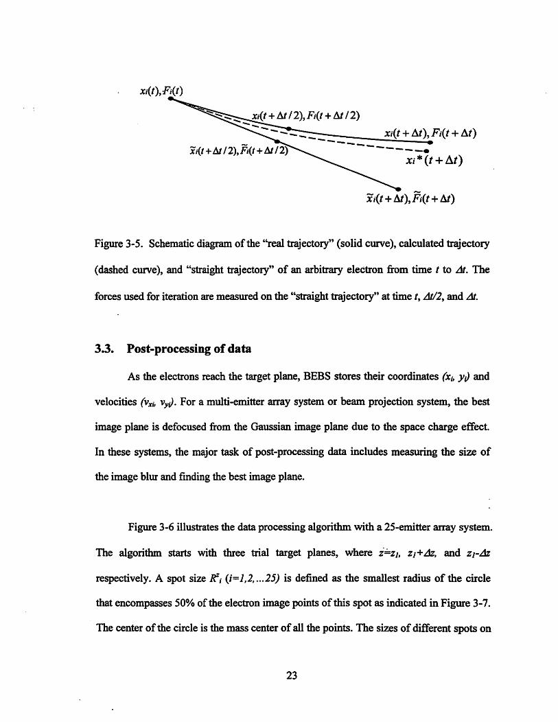
The dashed curve in Figure 3-5 is the trajectory of electron / calculated with the
above force. Its ending point is
Equation 3-5. xi*(t+At) » xi(t+At).
The validity of the above approximations are based on the assumption that all the
electron trajectories are "straight enough" within time At, in other words,
|ri(t+At) - ri{t+At)\<=threshold for every electron in the column. A larger value of
threshold will speed up the simulation with lower accuracy. On the other hand, a smaller
threshold tends to increase the accuracy at the expense of simulation time. The optimal
threshold at each beam current is obtained by lowering the threshold value until the spot,
size stops changing. For instance, threshold=le'6 is an appropriate choice for 30pA
beam current. It takes 200 to 400 times steps for an electron to travel through the column.
In the last step of each iteration, BEBS performs the threshold check. If the result is
negative for some electron. At will be halved to make the approximation more accurate.
On the other hand, if it works for two consecutive iterations. At will be double to speed
21
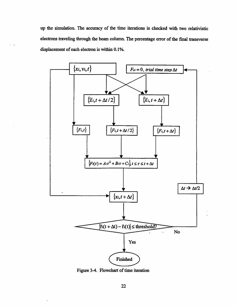
up the simulation. The accuracy of the time iterations is checked with two relativistic
electrons traveling through the beam column. The percentage error ofthe final transverse
displacement ofeach electron is within 0.1%.
Fxi = 0, trial time step At
{3c/,/ +A//2} {jci, t +A/}
y r
{Fut+At/2} {/'«,/+A/}
1 r y f \ r
{Fi(r) =AiT^ +BiT+Ci\ r<r</+A/
threshold?
Yes
^^F^shed^^Figure 3-4. Flowchart oftime iteration
22
At A//2
+ At / 2), Fi(t + At / 2)
_ Xi(t + At), Fi{t + A/)xi{t-¥Atl2),Fi{t+. , _
Xi *(t-\- At)
Xi{t + A/), Fi{t + At)
Figure 3-5. Schematic diagram ofthe "real trajectory" (solid curve), calculated trajectory
(dashed curve), and "straight trajectory" of an arbitrary electron from time t to At. The
forces used for iteration are measured on the "straight trajectory" at time t, At/2, and At.
3.3. Post-processing of data
As the electrons reach the target plane, BEBS stores their coordinates (Xi, yi) and
velocities (Vxb Vyi). For a multi-emitter array system or beam projection system, the best
image plane is defocused from the Gaussian image plane due to the space charge effect.
In these systems, the major task of post-processing data includes measuring the size of
the image blur and frnding the best image plane.
Figure 3-6 illustrates the data processing algorithm with a 25-emitter array system.
The algorithm starts with three trial target planes, where z=Z], zj+Az, and zj-Az
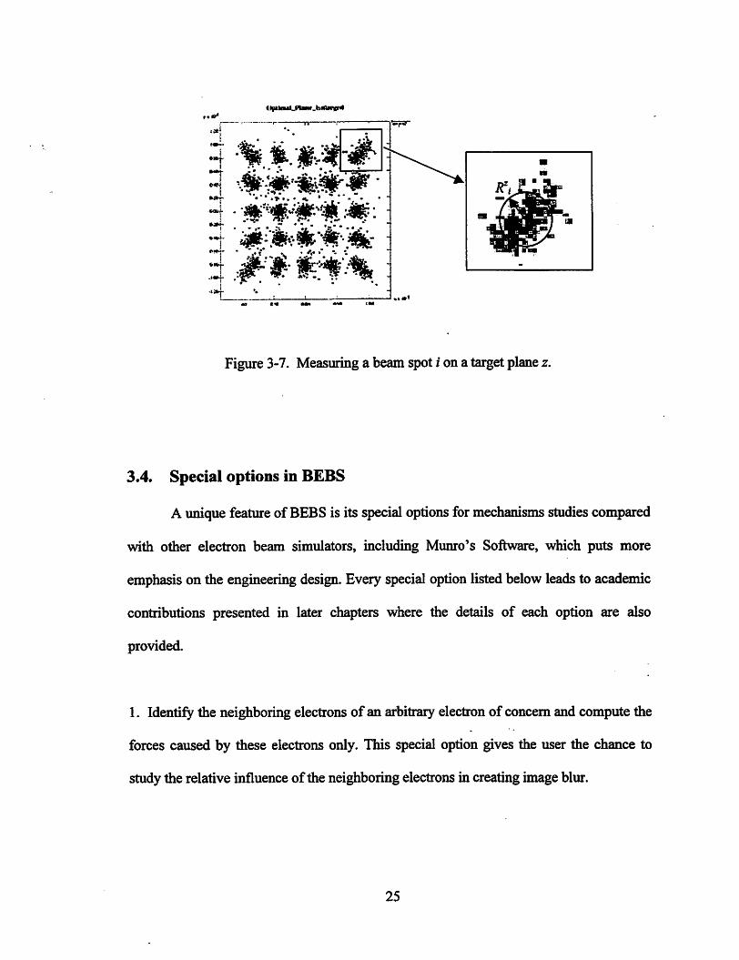
respectively. A spot size (i=l,2,...25) is defined as the smallest radius of the circle
that encompasses 50% of the electron image points of this spot as indicated in Figure 3-7.
The center of the circle is the mass center ofall the points. The sizes of different spots on
23
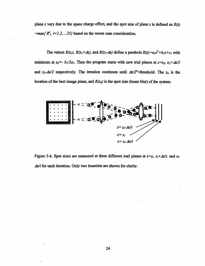
planez vary due to the spacecharge effect, and the spot size of plane z is defined as R(z)
=max{i=l,2, ,..25} based on the worse case consideration.
The values R(zj), R(zi-^Az), andR(z]-Az) define a parabola R(z)=a]Z^+bjz+cj with
minimum at Z2=- b]/2a]. Then the program starts with new trial planes at z=Z2, Z2+Az/2
and Z2-Az/2 respectively. The iteration continues until zl2/2"<threshold. The is the
locationofthe best image plane, and R(zi) is the spot size (beam blur) ofthe system.
z= ZrAz/i
z= Zi-Az/i
Figure 3-6. Spot sizes are measured at three different trail planes at z=Zi, Zi+Az/i, and zr
Az/i for each iteration. Only two beamlets are shown for clarity.
24
<l^li»aljnaMr_biAar)cnl
#"#• i!4'%mm
Figure 3-7. Measuring a beam spot i on a target planez.
3.4. Special options in BEBS
A unique feature of BEBSis its special options for mechanisms studies compared
with other electron beam simulators, including Munro's Software, which puts more
emphasis on the engineering design. Every special option listed below leads to academic
contributions presented in later chapters where the details of each option are also
provided.
1. Identify the neighboring electrons of an arbitrary electron of concern and compute the
forces caused by these electrons only. This special option gives the user the chance to
study the relative influence ofthe neighboring electrons in creating image blur.
25

2. Directly generate stochastic beam blurs insimulation through theuseof positrons. The
space blurs are completely eliminated in this case. This option is the first of its kind
among electron beam simulators and it gives users the capability to directly study the
stochastic blurs in any beam configurations. The details of this option together with
applications are covered on Chapter 5.
3. Separatethe beam blurs causedby electron trajectorydisplacements and those caused
by the electron velocity shifts through particle relocations. This option helps identify and
compare the blurs of the two causes.
4. Switch on/offCoulomb interactions indifferent regions in the beam column. Although
impossible to run in practice, these Gedanken experiments provide the chance to study
the blur contributions from different regions in the beam column.
5. Introduce lens aberration in either of the projection lenses to study their effects. The
choices of aberrations include astigmatism, axial astigmatism, coma, field curvature,
distortion, and spherical aberration.
6. Introduce positive ions in the beam column to study their influence on the beam blur.
Due to their large mass compared with electrons, the ions in the.colunm are assumed to
be stationary throughout the simulation.
26

3.5. Comparison with Munro's Software
In addition to the special options discussed in the previous section, a different
force computation algorithm is the other major difference between BEBS and Munro's
electron beam simulator. Instead of the FMM, Munro employs the Barnes-Hut (BH)
method.
3.5.1.^Bames-Hut algorithm
The BH algorithm involves two steps [69]. In the first step, all the particles in the
bunch are surrounded by a cubic box called the "root cell". This is subdivided into 8
smaller cells, until each particle has been assigned to a unique cell, as shown in Figure 3-
8. In the second step, the inter-particle forces are computed. To compute the force upon
particle P (see Figure 3-9), one starts from the root cell. Let L be its side length, and D
the distance from the centroid C of the particles in the cell to particle P. In Munro's
implementation of BH, if D>=L (as in Figure 3-9a), one computes the total force upon P
by assuming that all the charge in the cell is located at the centroid C. On the other hand,
if D<L (as in Figure 3-9b), then the cell is resolved into eight sub-cells and the procedure
is repeated recursively. To obtain the force upon each particle, the above procedure is
repeated for each point P where the particle is located. We will refer to this version ofBH
as the Munro type implementation.
27
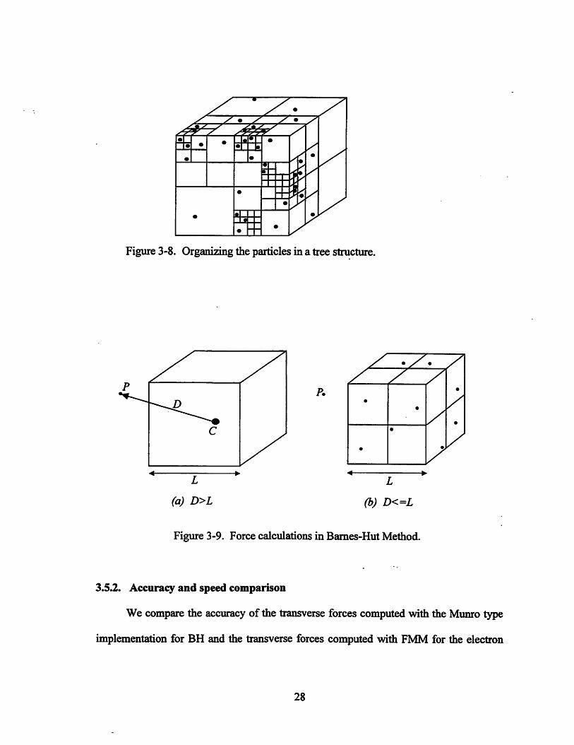
Figure 3-8. Organizing the particles in a tree structure.
L
(a) D>L
P.
L
(b) D<=L
Figure 3-9. Force calculations in Barnes-Hut Method.
3.5.2. Accuracy and speed comparison
We compare the accuracy of the transverse forces computed with the Munro type
implementation for BH and the transverse forces computed vrith FMM for the electron
28

bunch given in Figure 3-10. The electron bunch has the same geometry as the electron
bunchpassingthe crossover regionin Figure3-1 if the beam convergence angleis l.SmR,
AR
\1
7X~'L/3 •
n- • . \
y. •_j
Figure 3-10. The electron bunch used in the accuracy comparison between Barnes-Hut
and FMM. R=240fm and L=12mm.
The simulation computes the transverse forces Fx and Fy on an arbitrary electron
located in the 4mm part in the middle of the electron bimch with (a) FMM, (b) BH, and
(c) direct calculation of forces from every other electron in the bunch. The forces
computed with FMM and BH are compared with forces calculated directly and the
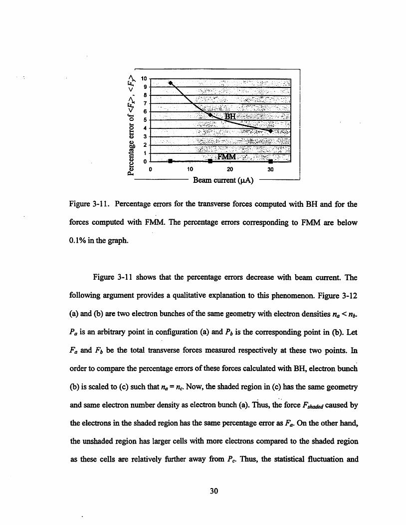
percentage errors for FMM and BH are presented in Figure 3-11.
The simulation shows that the transverse forces computed with BH on average
have 9% errors compared the forces predicted by direct calculations at 5pA beam current.
The percentage error tends to decrease as the beam current increases. The error for the
forces calculated with FMM, on the other hand, is always within 0.1% for SpA to 30pA.
29
V
*-
2V
4)
§>"Sa>
2a> 10 20 30
- Beam current ()iA)
Figure 3-11. Percentage errors for the transverse forces computed with BH and for the
forces computed with FMM. The percentage errors corresponding to FMM are below
0.1% in the graph.
Figure 3-11 shows that the percentage errors decrease with beam current. The
following argument provides a qualitative explanation to this phenomenon. Figure 3-12
(a) and (b) are two electron bunches of the same geometry with electron densities ria< ni,.
Pa is an arbitrary point in configuration (a) and Pb is the corresponding point in (b). Let
Fa and Fb be the total transverse forces measured respectively at these two points. In
order to compare the percentage errors of these forces calculated with BH, electron bimch
(b) is scaled to (c) such that Ha - ric. Now, the shaded region in (c) has the same geometry
and same electron number density as electron bunch (a). Thus, the force Fshaded caused by
the electrons in the shaded region has the same percentage error as Fa- On the other hand,
the unshaded region has larger cells with more electrons compared to the shaded region
as these cells are relatively further away from Pc. Thus, the statistical fluctuation and
30

percentage error of Fumhaded calculated with BH is smaller thanthatof Fshaded- Therefore,
The total transverse force Fc = Fshaded + Fu„shaded has less percentage errors than Fa. In
otherwords, the percentage errors of forces decrease at highercurrent density.
• •
• •• •
(a)\
Pa
• • • •* • •• • • •»*.. • • .* »•».«>v*»
(b) Pi
•• ••
• •
• •• • • •
• • • I
• • •• • •
• •
• • • •
• •
• •
• •
(c)
Figure 3-12. Electron bunch (a) and bunch (b) with electron densities ria < ny and the
scaled electron bunch (c) with ric - ria.
Errors in the force calculations certainly influence the accuracies of the final beam
blur. The following back-of-the-envelope calculation provides a rough estimate of the
percentage error for the corresponding beam blurs based on physical intuition. The
accuracy ofthe estimates requires more rigorous studies.
Results given in the next chaptershow that 90% ofthe beam blur is caused by the
transverse forces in the region within 200mm of the crossover at 5|iA beam current. The
31
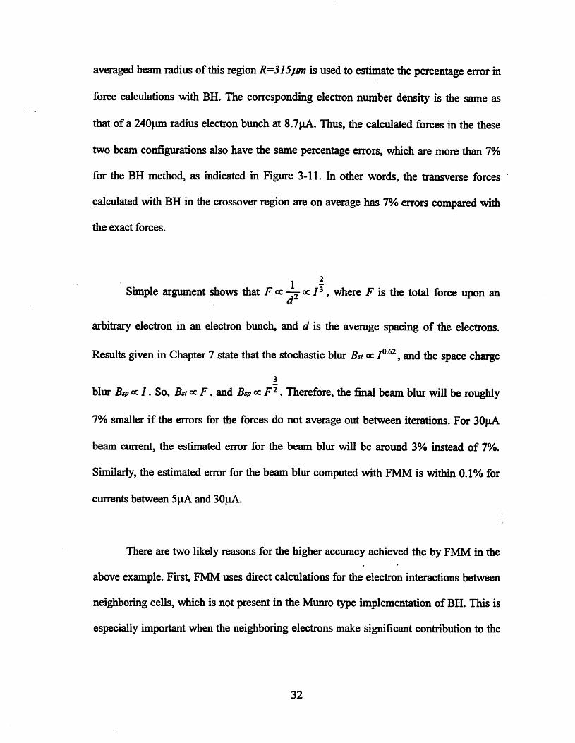
averaged beam radius of this region R=315jLmi is used to estimate the percentage error in
force calculations with BH. The corresponding electron number density is the same as
that of a 240|jm radius electron bunch at 8.7pA. Thus, the calculated forces in the these
two beam configurations also have the same percentage errors, which are more than 7%
for the BH method, as indicated in Figure 3-11. In other words, the transverse forces
calculated with BH in the crossover region are on average has 7% errors compared with
the exact forces.
1 -Simple argument shows that Fcc—^qc P, where F is the total force upon an
d
arbitrary electron in an electron bunch, and d is the average spacing of the electrons.
Results given in Chapter 7 state that the stochastic blur Bst oc 7®^^, and the space charge
3
blur BspfXil. So, BstccF, and BspccF^. Therefore, the final beam blur will be roughly
7% smaller if the errors for the forces do not average out between iterations. For 30|iA
beam current, the estimated error for the beam blur will be around 3% instead of 7%.
Similarly, the estimated error for the beam blur computed with FMM is within 0.1% for
currents between 5pA and 30pA.
There are two likely reasons for the higher accuracy achieved the by FMM in the
above example. First, FMM uses direct calculations for the electron interactions between
neighboring cells, which is not present in the Munro type implementation of BH. This is
especially important when the neighboring electrons make significant contribution to the
32
total transverse force. Secondly, FMM includes up to the 5^ term in the spherical
harmonic expansion whilethe BH implemented aboveonly uses the monopole term.
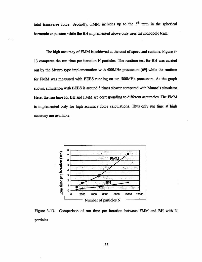
The high accuracy of FMMis achieved at the cost ofspeedandruntime. Figure3-
13 compares the run time per iteration N particles. The runtime test for BH was carried
out by the Munro type implementation with 400MHzprocessors [69] while the runtime
for FMM was measured with BEBS running on ten 500MHz processors. As the graph
shows, simulation with BEBS is around 5 times slower compared with Mimro's simulator.
Here, the run time for BH and FMM are corresponding to different accuracies. The FMM
is implemented only for high accuracy force calculations. Thus only run time at high
accuracy are available.
o0)C/3
GO
"eS
a>
^ 0 2000 4000 6000 8000 10000 12000
Number ofparticles N ^ '
Figure 3-13. Comparison of run time per iteration between FMM and BH with N
particles.
33

4 Beam Blur Contributions in Multi-emitter Array
Systems
4.0. Introduction
This chapter first presents how beam blur contributions vary along the optical axis
in Section 4.1. Next it will discuss how the electrons from the same beamlet and electrons
from different beamlets interact and produce beam blur in Section 4.2. The summation
rule of the blur contributions will also be presented in this section. The topics covered in
this chapter were first investigated by the author and Neureuther [25].
4.1. Blur contribution along the optical axis
Studying how Coulomb interactions in different regions contribute to the final
spot size helps identify the regions producing most of the beam blur. This will provide
insight to new strategies for beam-blur reduction. Figure 4-1 shows the schematic
diagram for the simulated 4X demagnification system. The emitter array consists of
twenty-five emitters with 200{im spacing. The illumination convergence angle of each
beamlet is Gaussian distributed with standard deviation equal to a. The whole colurrm is
divided into eleven labeled regions.
34
10 11
320 360 400
z(mm)
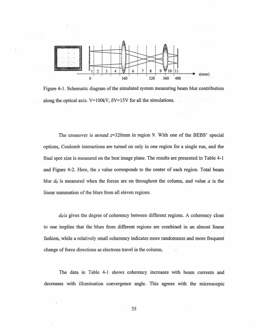
Figure 4-1. Schematic diagram of the simulated system measuring beam blur contribution
along the optical axis. V=100kV, 5V=15V for all the simulations.
The crossover is around z=320mm in region 9. With one of the BEBS' special
options, Coulomb interactions are turned on only in one region for a single run, and the
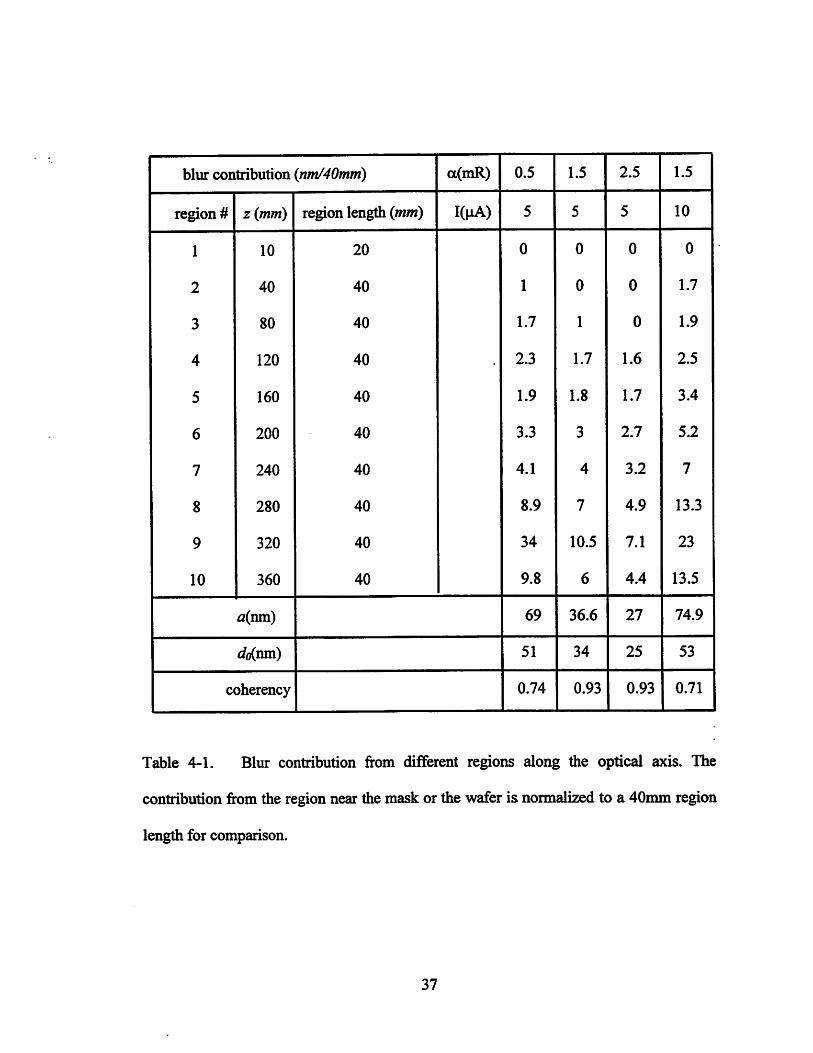
final spot size is measured on the best image plane. The results are presented in Table 4-1
and Figure 4-2. Here, the z value corresponds to the center of each region. Total beam
blur do is measured when the forces are on throughout the column, and value a is the
linear summation of the blurs from all eleven regions.
dt^a gives the degree of coherency between different regions. A coherency close
to one implies that the blurs from different regions are combined in an almost linear
fashion, while a relatively small coherency indicates more randomness and more frequent
change of force directions as electrons travel in the column.
The data in Table 4-1 shows coherency increases with beam currents and
decreases with illumination convergence angle. This agrees with the microscopic

interpretation that the stochastic forces make more directional changes at higher electron
densities.
Figure 4-2 and Figure 4-3 show that the contribution from the crossover region
(region 9) becomes more significant at smaller convergence angles and at higher current
beam currents. Numerically, this contribution is roughlyproportional to I/a. On the other
hand, the regions near the mask and the wafer contribute little, in spite of the high
electron densities.
36
blur contribution {nm/40mm) a(mR) 0.5 1.5 2.5 1.5
region # z {mrri) region length {mm) I(pA) 5 5 5 10
1 10 20 0 0 0 0
2 40 40 1 0 0 1.7
3 80 40 1.7 1 0 1.9
4 120 40 2.3 1.7 1.6 2.5
5 160 40 1.9 1.8 1.7 3.4
6 200 40 3.3 3 2.7 5.2
7 240 40 4.1 4 3.2 7
8 280 40 8.9 7 4.9 13.3
9 320 40 34 10.5 7.1 23
10 360 40 9.8 6 4.4 13.5
a(nm) 69 36.6 27 74.9
</o(nm) 51 34 25 53
coherency 0.74 0.93 0.93 0.71
Table 4-1. Blur contribution from different regions along the optical axis. The
contribution from the region near the mask or the wafer is normalized to a 40mm region
length for comparison.
37

35
30
e25^ 20s2 153
ffi 10
5
0
100 200 300
z(mm)
400
•alpha=0.5mR
'alpha=1.5mR
alpha=2.5mR
Figure4-2. Beam blur contributionalong the optical axis at different convergence angles.
Here I = 5/jA.
I=10liA
z(mm)
Figure 4-3. Beam blur contribution along the optical axis at different beam currents.
Here beam convergence angle a=L5mR.
38
4.2. Inter-beamlet, intra-beamlet electron interactions and the
summation rule
4.2.0. Mask configurations
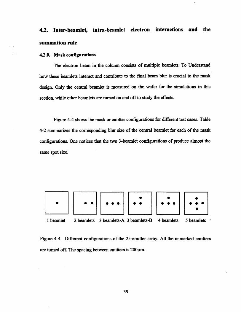
The electron beam in the column consists of multiple beamlets. To Understand
how these beamlets interact and contribute to the final beam blur is crucial to the mask
design. Only the central beamlet is measured on the wafer for the simulations in this
section, while other beamlets are tumed on and off to study the effects.
Figure 4-4 shows the mask or emitterconfigurations for different test cases. Table
4-2 summarizes the corresponding blur size of the central beamlet for each of the mask
configurations. One notices that the two 3-beamlet configurations of produce almost the
same spot size.
1 beamlet 2 beamlets 3 beamlets-A 3 beamlets-B 4 beamlets 5 beamlets '
Figure 4-4. Different configurations of the 25-emitter array. All the unmarked emitters
are tumed off. The spacing between emitters is 200pm.
39
alpha(mR) beamlets 1 2 3-A 3-B 4 5
0.5 26 46 60 61 69 78
spot size D (nm)1.5 10 22 30 30 35 40
2.5 5 15 20 22 25.5 28
0.5 676 2116 3600 4761 6084
spot area D^(nm^)1.5 100 484 900 1225 1600
2.5 25 225 400 650.3 784
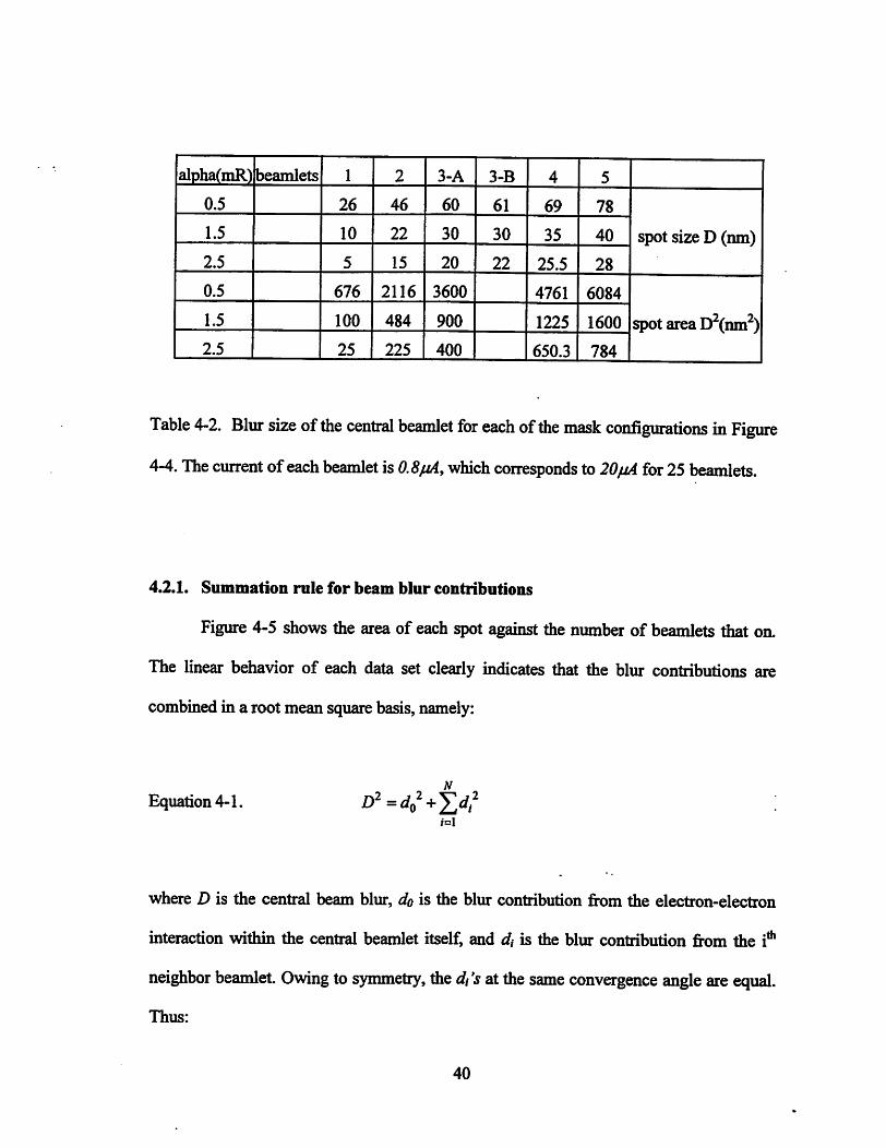
Table 4-2. Blur size ofthe central beamlet for each ofthe mask configurations inFigure
4-4. The current of each beamlet is which corresponds to 20^ for25 beamlets.
4.2.1. Summation rule for beam blur contributions
Figure 4-5 shows the area of each spot against the number of beamlets that on.
The linear behavior of each data set clearly indicates that the blur contributions are
combinedin a root mean square basis, namely:
Equation 4-1.n
2 . j2
i=I
where D is the central beam blur, do is the blur contribution from the electron-electron
interaction within the central beamlet itself, and di is the blur contribution from the i***
neighbor beamlet. Owing to symmetry, the dis at the same convergence angle are equal.
Thus:
40
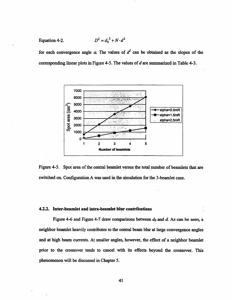
Equation 4-2. =dQ +N'
for each convergence angle a The values of (f can be obtained as the slopes of the
corresponding linear plots in Figure 4-5. The values ofd are summarized in Table 4-3.
6000
S 3000
O 2000
- 1000
2 3 4
Number of beamlets
'alpha=0.5mR
•alpha=1.5mR
alpha=2.5mR
Figure 4-5. Spot area of the central beamlet versus the total number ofbeamlets that are
switched on. Configuration A was used in the simulation for the 3-beamlet case.
4.2.2. Inter-beamlet and intra-beamlet blur contributions
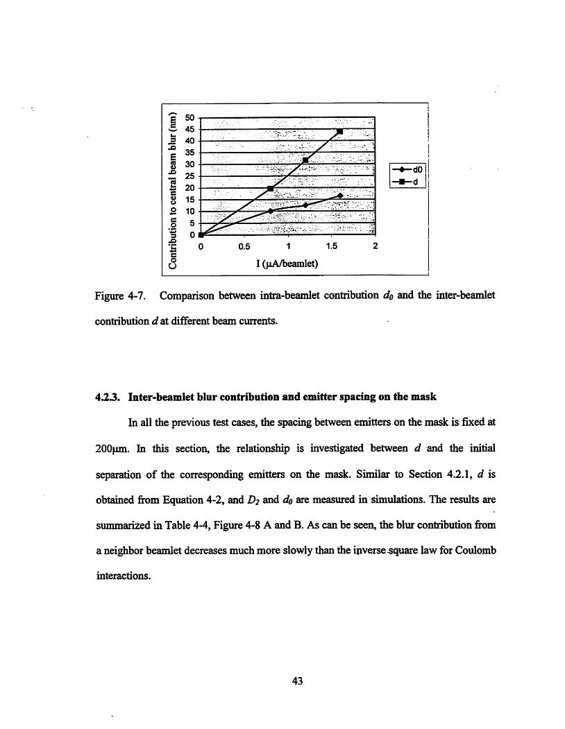
Figure 4-6 and Figure 4-7 draw comparisons between do and d. As can be seen, a
neighbor beamlet heavily contributesto the central beam blur at large convergence angles
and at high beam currents. At smaller angles, however, the effect of a neighbor beamlet
prior to the crossover tends to cancel with its effects beyond the crossover. This
phenomenon will be discussed in Chapter 5.
41

1=0.8
CuA/beamlet) alDha=1.5 CmR^
aloha fmR) dftfnm) d fnm) I CuA/beamlefi dnTmn^ dfnm'l
0.5 26 38 0.8 10 19.6
1.5 10 19.6 1.2 12.5 31.6
2.5 5 14 1.6 16.5 43.8
Table 4-3. Beam blur contribution d from a neighbor beamlet and the blur contribution
do from the central beamlet itself, d is obtained from Equation 4-2.
40 jECBO 35
1 30 •
eo 25 •
o E" 20
3 3 15 -•C -Oo33
10 ••
A 5 •
Co 0 f
o0 0.5 1 1.5 2
alpha (mR)
2.5
•d
-do
Figure 4-6. Comparison between intra-beamlet contribution do and the inter-beamlet
contribution d at different convergence angles.
42
S 30
is 20
B 10
0.5 1 1.5
I (^A/beamlet)
-dOl!
Figure 4-7. Comparison between intra-beamlet contribution do and the inter-beamlet
contribution d at different beam currents.
4J23. Inter-beamlet blur contribution and emitter spacing on the mask
In all the previous test cases, the spacing between emitters on the mask is fixed at
200pm. In this section, the relationship is investigated between d and the initial
separation of the corresponding emitters on the mask. Similar to Section 4.2.1, d is
obtained fi'om Equation 4-2, and D2 and do are measured in simulations. The results are
summarized in Table 4-4, Figure 4-8 A and B. As can be seen, the blur contribution firom
a neighbor beamlet decreases much more slowly than the inverse-square law for Coulomb
interactions.
43

Distance
(grid) 0.5
I=0.8|xA/beamlet
1 2
, a=1.5mR
3 4 5 6 7
D2 (nm) 24 22 21.5 21 20 18.5 17 16
dO (nm) 10 10 10 10 10 10 10 10
d (nm) 21.8 19.6 19 18.5 17.3 15.6 13.7 12.5
Distance
(grid) 0.5
I=0.8|xA/beamlet, a=2.5mR
1 2 3 4 5 6 7
D2 (nm) 16 15 14 13.5 13 12 11.5 11
dO (nm) 4 5 5 5 5 5 5 5
d (nm) 15 14 13 12.5 12 11 10.4 9.8
Distance
(grid) 0.5
I=1.2^A^eamlet, a=1.5mR
12 3 4 5 6 7
D2 (nm) 37.5 34 30 27.5 26 25 24 23
dO (nm) 12.5 12.5 12.5 12.5 12.5 12.5 12.5 12.5
d (nm) 35.4 35.4 27.3 24.5 22.8 21.7 20.5 19.3
Table 4-4. Beam blur contribution d caused by inter-beamlet electron interactions varies
with the distance between the emitters on the mask. A grid here equals 200|jm.
44

25
» 20
»(0
E 150
B§ 10O)c
1 5&
(A) I=0.8|iA/beainlet
—alpha=1.5mR
• alpha=2.5mR
4
d (nm)
(B) a=1.5mR
2 4 6
Spacing on the mask (grid)
l=0.8uA/beamlet
1=1.2uA/beamlet
Figure 4-8. Beam blur contribution d from a neighbor beamlet decreases with the
corresponding emitter spacing on the mask. One grid equals 200)xm separation on the
mask.
45

4.3. Conclusions
Studies showthatbeamblur is mostlyproduced in the crossover region in a multi-
emitter array system, which implies that blur reduction techniques should focus on
interactions in this region. Meanwhile, the blur contributions caused by inter-beamlet
electron interactions dominate over those caused by intra-beamlet electron interactions,
especially at large convergence angles. Further study is needed in order to find efficient
ways to isolateand manipulate inter-beamlet interactions in an experimental setup.
Simulation results demonstrate that the beam blur contributions from different beamlets
can be combined on a root mean square basis.
46
5 Stochastic Goulomb Interactions and
Neighboring Electrons
5.0. Introduction
Mkrtchyan's Nearest-Neighbor Theory [6] is one of the analytical models used to
study stochastic interactions in e-beam lithography. This chapter provides the
methodology to verify one of Mkrtchyan's basic assumptions, namely that the stochastic
force upon each electron in a beam column is dominated by the contribution from the
nearest neighbor electron. Section 5.1 introduces the basic setup of the test system.
Section 5.2 discusses the number of neighboring electrons in different regions along the
optical axis. Section 5.3 addresses the issue of how the number of neighboring electrons
affects the transverse stochastic forces. The reader may refer to Chapter 2 for a brief
introduction to the analytical models on the electron stochastic effects.
5.1. System setup
A basic test geometry of a crossover in a lens free region equidistant between two
lenses was used to explore the nature of the electron-electron interactions. The test beam
geometry is shown in Figure 5-1. The crossover is midway (at 100mm) in the 200mm
lens free analysis domain. The electron emitter for this study was idealized to inject
47

electrons withall the same energy (6E= 0) andthe angle wascomputed from the random
lateral position so that each electron if undeflected by others would pass through the
mathematical crossover (6a = 0). An ideal lens was assumed to follow the simulation
domain, which focused the crossover to a point on an image plane 100mm beyond the
simulation domain. This lens, whose focal length is independent of electron energy,
provides a means of directly observing beam blur due to electron-electron Coulomb
interactions. For the studies shown below, the beam energy was lOOkV and the radius of
the initial beam was 1mm. The simulation domain was a 200mm cylindrical tube with a
1mm radius.
Ideal Emitter
Beam profile
Interaction region
Ideal lens
Force free region
100mm 100mm 100mm
Figure 5-1. Test beam geometry. The systemparameters are: V=l00kV, AE=0, r= Imm,
femUKr^l00mm,f^^=50mm.
48
Image plane
/
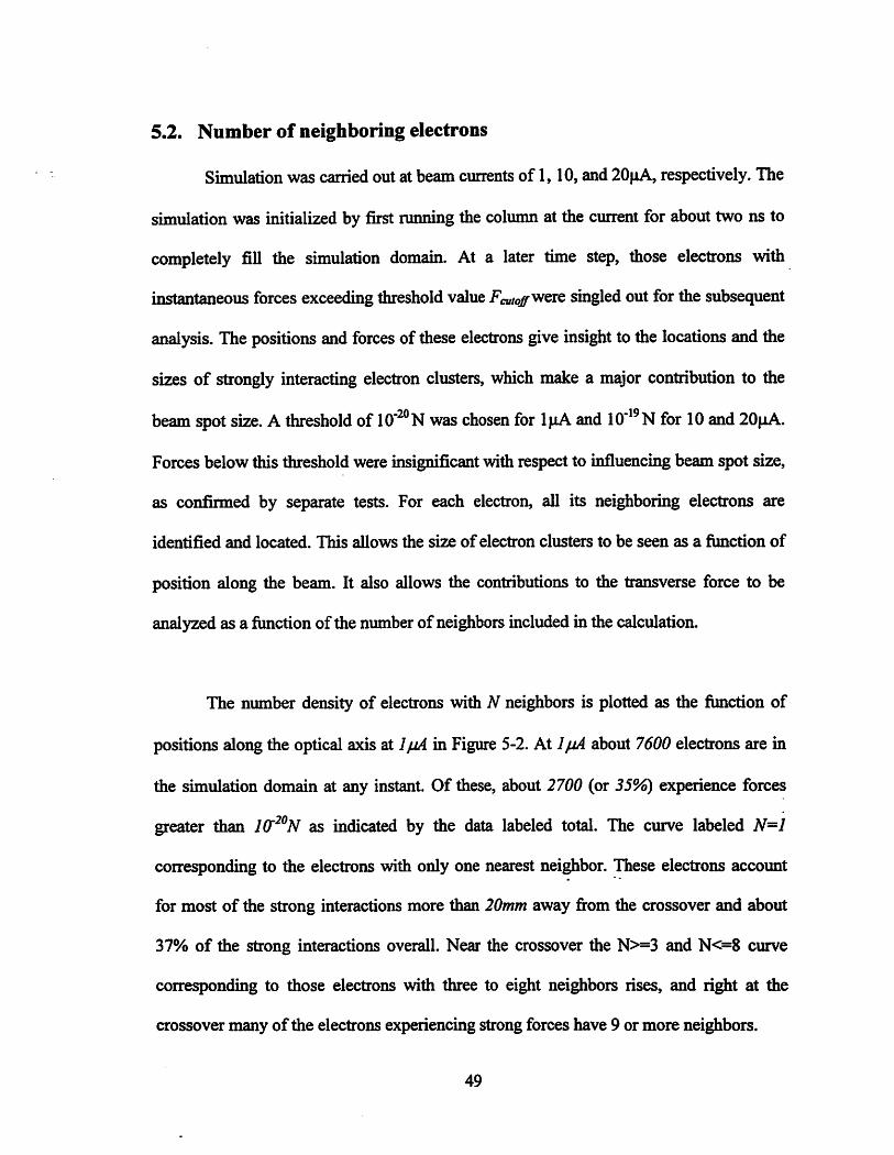
5.2. Number of neighboring electrons
Simulation was carried out at beam currentsof 1,10, and 20fiA, respectively. The
simulation was initialized by first running the column at the current for about two ns to
completely fill the simulation domain. At a later time step, those electrons with
instantaneous forces exceeding thresholdvalue Fcato#were singled out for the subsequent
analysis. The positions and forces of these electrons give insight to the locations and the
sizes of strongly interacting electron clusters, which make a major contribution to the
beam spot size. Athreshold of10*^®Nwas chosen for IpA and 10"^^Nfor 10 and 20pA.
Forces below this threshold were insignificant with respect to infiuencingbeam spot size,
as confirmed by separate tests. For each electron, all its neighboring electrons are
identified and located. This allows the size ofelectron clusters to be seen as a fimction of
position along the beam. It also allows the contributions to the transverse force to be
analyzed as a fimctionof the numberof neighbors includedin the calculation.
The number density of electrons with N neighbors is plotted as the fimction of
positions along the optical axis at 7/Z/4 in Figure 5-2. At about 7600 electrons are in
the simulation domain at any instant. Of these, about 2700 (or 35%) experience forces
greater than as indicated by the data labeled total. The curve labeled N=^l
corresponding to the electrons with only one nearest neighbor. These electrons accoimt
for most of the strong interactions more than 20mm away fi:om the crossover and about
37% of the strong interactions overall. Near the crossover the N>=3 and N<=8 curve
corresponding to those electrons with three to eight neighbors rises, and right at the
crossover many of the electrons experiencing strong forces have 9 or more neighbors.
49

s£
oo.M
so
N>=9
N>=3 and N<=8
S 20
4>
E
0 0.02 0.04 0.06 0.08 0.1 0.12 0.14 0.16 0.18 0.2
2(m)
Figure 5-2.Number of neighbors electrons vs. axial position for 1=1pA and Fcutoff=10'̂ °N.
Figures 5-3 and 5-4 showthe number density of electrons with N neighbors along
the column for beam current increasing to 10 and 20juA, The curves are quite similar in
shape to that for 1 pA. However, note that the vertical axis has been scaled proportional
to beam current. The area is about 9,062 electrons or 12% of the 76,000 electrons in a
lOjuA beam. The decrease in the cases with less than 9 neighbors at the crossover is quite
noticeable. As might be expected, the shape of these curves generally follows the number
of electrons expected to be within a sphere with a radius of 48 um. Fortunately, this also
indicates that the observed trends are likely scaleable to slightly lower force thresholds at
which as much as 30% of the electrons undergo transverse-displacements and produce
beam blur.
50

400
g 350
tM300
0)
m 250(3OUU 200
Cm 150OM
JD 100
2 50
0
1 r/N>=9
N=1 / \ . N>=3andN<s=8
A
0.02 0.04 0.06 O.OS 0.1 0.12 0.14 0.16 0.18 0.2z(m)
Figure 5-3. Number ofelectrons with N neighbors vs. axial position for I=10|xA and
Fa„<ff=10r"N.
800•
700 4 I\ •
I Total600
500 r ^ N>=9400
fI ✓ N>=3 andN<=S
300 N=lv / \/200
J
100
0
y AW
a.M
G
so
"oCm
o
a>
BG
2
0 0.02 0.04 0.06 0.08 0.1 0.12 0.14 0.16 0.18 0.2z(m)
Figure 5-4. Number of electrons with N neighbors vs. axial position for I=20|iA and
Fa.usr=i(r"N.
51
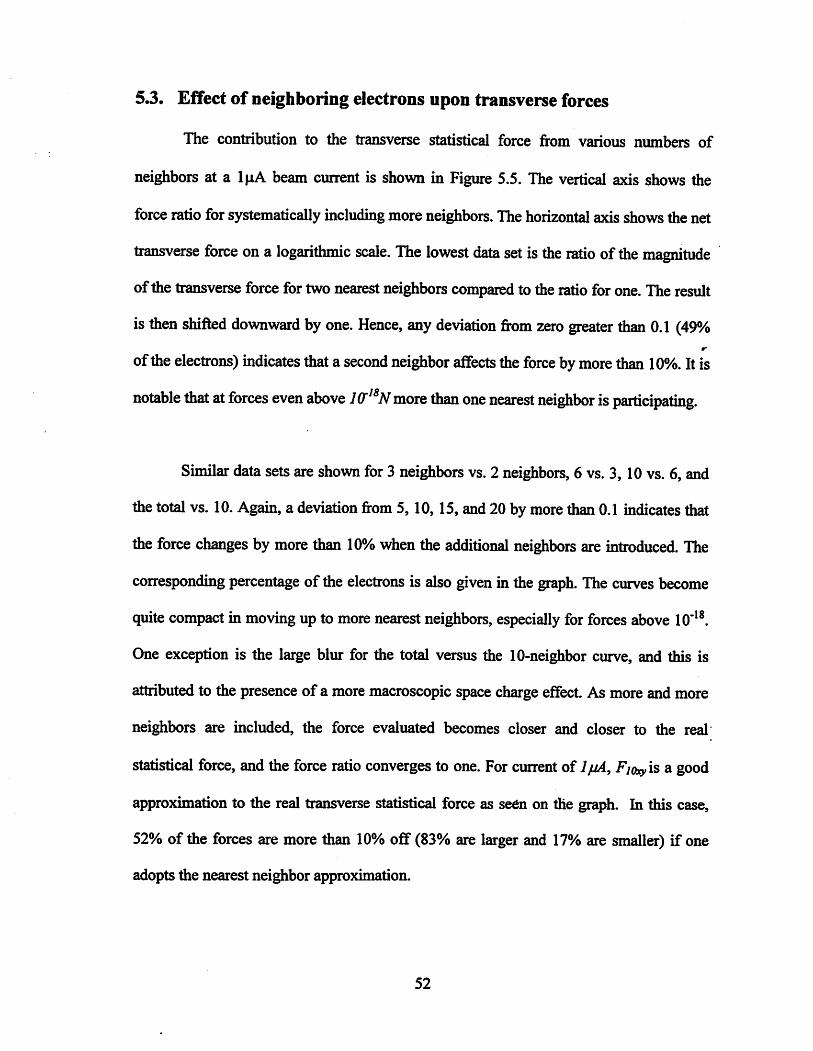
5.3. Effect of neighboring electrons upon transverse forces
The contribution to the transverse statistical force from various numbers of
neighbors at a IjiA beam current is shown in Figure 5.5. The vertical axis shows the
force ratio for systematically includingmore neighbors.Hie horizontal axis shows the net
transverse force on a logarithmic scale. The lowest data set is the ratio of the magnitude
ofthe transverse force for two nearest neighbors compared to the ratio for one. The result
is then shifted downward by one. Hence, any deviation from zero greater than 0.1 (49%r
of the electrons) indicates that a second neighbor affects the force bymore than 10%. It is
notable that at forces even above 1(T^^Nmore than one nearest neighbor is participating.
Similar data sets are shown for 3 neighbors vs. 2 neighbors, 6 vs. 3,10 vs. 6, and
the total vs. 10.Again, a deviation from 5,10,15, and 20 by more than 0.1 indicates that
the force changes by more than 10% when the additional neighbors are introduced. The
corresponding percentage of the electrons is also given in the graph. The curves become
quite compact in moving up to more nearest neighbors, especially for forces above 10"'®.
One exception is the large blur for the total versus the 10-neighbor curve, and this is
attributed to the presence of a more macroscopic space charge effect. As more and more
neighbors are included, the force evaluated becomes closer and closer to the real
statistical force, and the force ratio converges to one. For current of 7/z4, Fioxyis a good
approximation to the real transverse statistical force as seen on the graph. In this case,
52% of the forces are more than 10% off (83% are larger and 17% are smaller) if one
adopts the nearest neighbor approximation.
52

2u
2o
Fxy/F,0xy+19 •
FlOxj/F^xy .(11%)
^exy^licy-^^(27%)F3xy^2xy + 4(32%)
F2xy^xy+ 1(49%)
-20 -19.S -19 -18.5 -18 -17.5 -17 -16.5 -IB -15.5 -15LOG,o{/VW)
Figure 5-5. Effectof neighboring electrons upontiansverse forces for 1=1|xA and
/^««.#=10- '̂'N.
Figures 5-6 and Figure 5-7 show the contribution to the transverse statistical force
from various numbers of neighbors at 10 to 20 \iA. An order of magnitude increase in
beam current causes a two order ofmagnitude translation of the data set to higher forces.
This is because the tenfold increase in beam current causes a tenfold decrease in the
average spacing, which results in a two order of magnitude increase in the typical force.
The spread in the data beyond a deviation of 0.1 is now much greater, and the increased
spread becomes particularly noticeable even when 6 and 10 neighbors are added. At
lOpA it is likely the norm rather than the exception to have several nearest neighbors
contributing to the force when passing through the crossover. Since multiple neighbors
become important about 10mm prior to the ideal crossover where the lOjuA current
corresponds toa current density of30mA/cm^, this current density might serve asa rule of
thumb for when multiple neighbor contributions are completely dominating.
53

-:A?-
FVF,(„,+ 19
F|0xy/F6xy+14(22%)
F6VF3xy+930%)
i4% ♦«*» ♦
F3xy^2xy +4
^ '*2x/l*lxy"'" 1
-19 -18.5 -18 -17.5 -17 -18.5 -IB -15.5J LOG,o(F^;
Figure 5-6. Effect of neighboring electrons upon transverse forces for 1=1OpA and
-19 -1B.S -18 -17.5 -17 -1B.S -IB -15.5 -IS
Px/^lOxy"^
M0xy^6xy'̂ 1^
1 ii.i:r.-j<rn€»<ir<rr Wl^3xy + 9
LOG,o(F;^W)
Figure 5-7. Effect of neighboring electrons upon transverse forces for I=20pA and
iW=10-"N.
54
5.4. Conclusions
Analysis of a basic crossovershowedthat strong transverse-deflection forces were
associated with high particle density. More importantly, interactions with multiple rather
than nearest neighbors almost immediatelybecame the norm rather than the exception. In
practical systems where crossovers are not ideal, the current density might be used as a
guide, with strong multiple neighbor interactions being observed at lOmA/cm^ and clearly
dominant at SOmAJcrrf. The corresponding typical electron inter-particle spacings are
62fm and 43respectively.
55

6 Structure ofStochastic Coulomb Interactions
6.0. Introduction
Traditionally, the stochastic beam blurs have been considered as random and
uncorrectable, until a puzzling result was discovered. Jansen [26] predicted that the
homocentric beam with a crossover and the homocentric parallel beam in Figure 6-1
produce the same spot size in spite of the high electron densities in the crossoverregions.
The prediction was later confirmed in simulations [41] [42]. To explain this puzzling
result, Jansen suggested that some cancellation mechanism in stochastic interactions
reduces the final beam blur in the configuration with a crossover. Nevertheless, the
sophisticated mathematical formulation of his model failed to give convincing physical
insight into this problem.
56
ElectronWafers
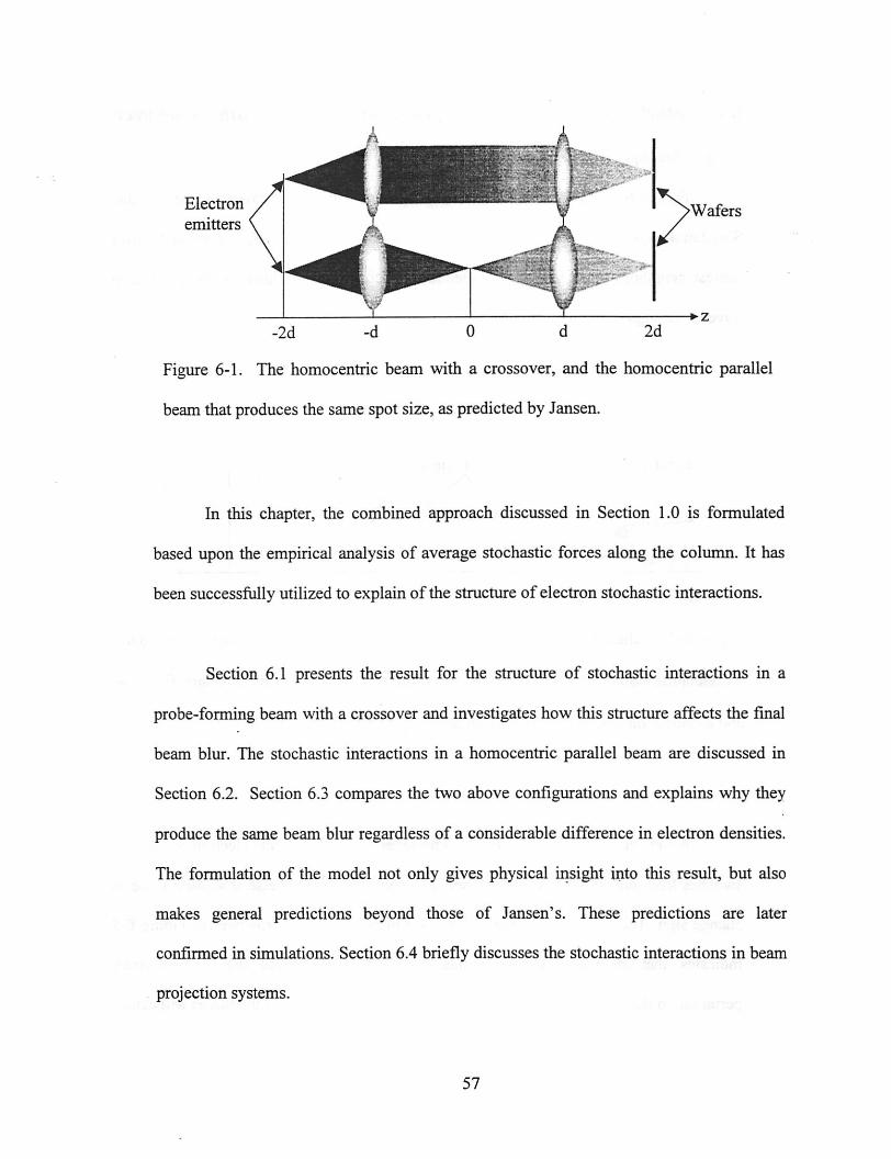
Figure 6-1. The homocentric beam with a crossover, and the homocentric parallel
beam that produces the same spot size, as predicted by Jansen.
In this chapter, the combined approach discussed in Section 1.0 is formulated
based upon the empirical analysis of average stochastic forces along the column. It has
been successfully utilized to explain of the structure ofelectron stochastic interactions.
Section 6.1 presents the result for the structure of stochastic interactions in a
probe-forming beam with a crossover and investigates how this structure affects the final
beam blur. The stochastic interactions in a homocentric parallel beam are discussed in
Section 6.2. Section 6.3 compares the two above configurations and explains why they
produce the same beam blur regardless of a considerable difference in electron densities.
The formulation of the model not only gives physical iiisight into this result, but also
makes general predictions beyond those of Jansen's. These predictions are later
confirmed in simulations. Section 6.4 briefly discusses the stochastic interactions in beam
projection systems.
6.1. Stochastic interactions in a probe-forming beam with a crossover
6.1.0. Stochastic force upon a single electron
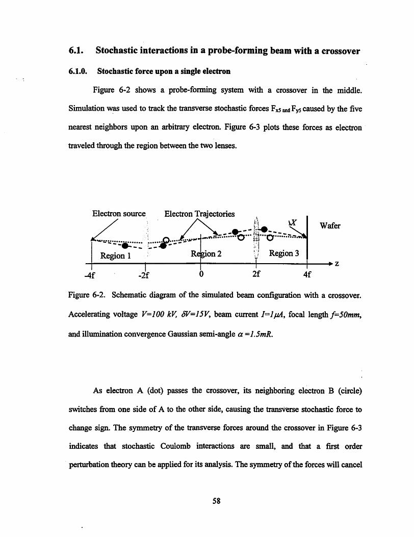
Figure 6-2 shows a probe-forming system with a crossover in the middle.
Simulation was used to track the transverse stochastic forces Fxs and Fys caused by the five
nearest neighbors upon an arbitrary electron. Figure 6-3 plots these forces as electron
traveled through the region between the two lenses.
Electron source
\X
ElectronTrajectories ,Wafer
Region 1 Region 2 Region 3
-4f -2f 0 2f 4f
Figure 6-2. Schematic diagram of the simulated beam configuration with a crossover.
Accelerating voltage V=100 kV, SV=15V, beam current 1=1ptA, focal lengthf=50mm,
and illumination convergence Gaussian semi-angle a =L5mR,
As electron A (dot) passes the crossover, its neighboring electron B (circle)
switches from one side of A to the other side, causing the transverse stochastic force to
change sign. The symmetry of the transverse forces around the crossover in Figure 6-3
indicates that stochastic Coulomb interactions are small, and that a first order
perturbation theory can be applied for its analysis. The symmetry of the forces will cancel
58
out the blur contribution caused by velocity shift only while the blur caused by trajectory
shift survives.
8
6
*
1^mP 0
X to*
[ ffi
L/ V\
1 Fys
(%%
^%
A-j
•0.1 •0.05 0Z|m)
0.05 0.1
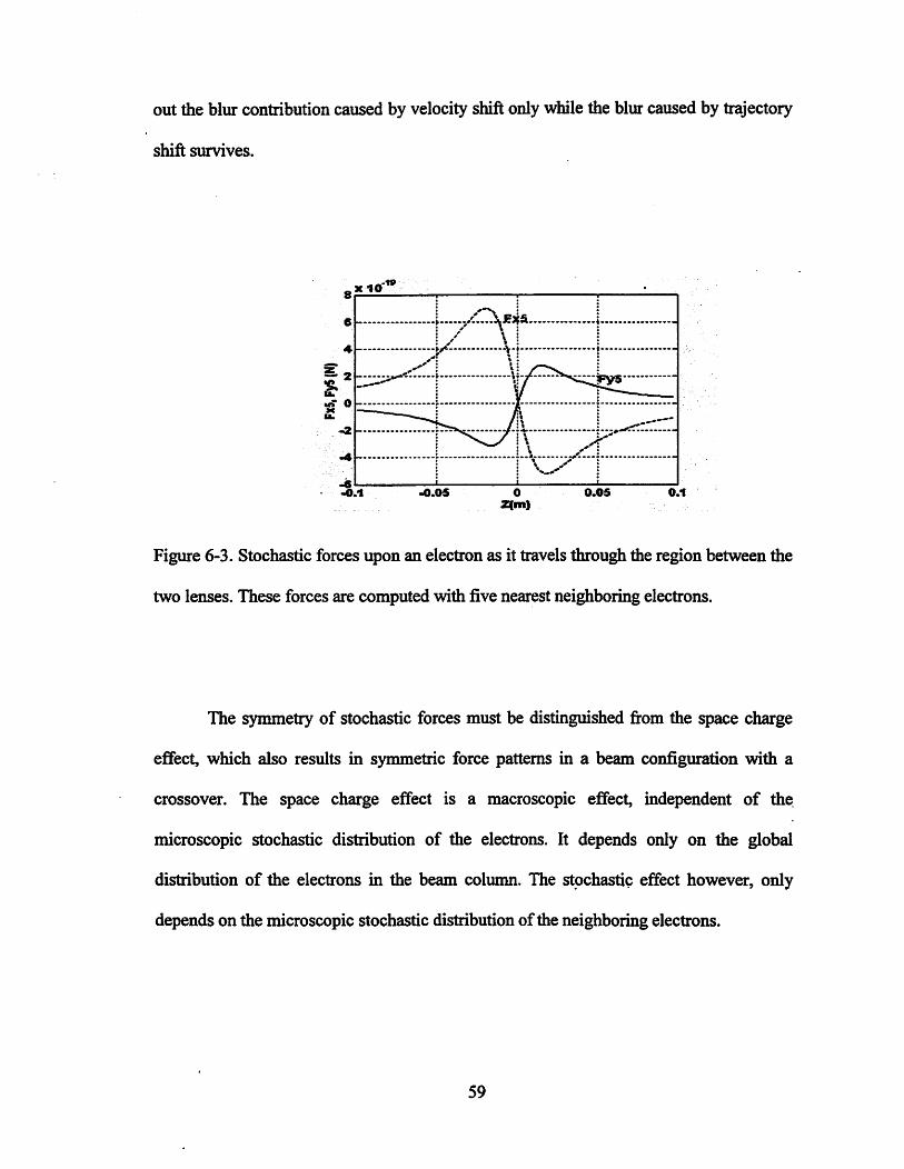
Figure 6-3. Stochastic forces upon an electron as it travels through the region between the
two lenses. These forces are computed with five nearest neighboring electrons.
The symmetry of stochastic forces must be distinguished from the space charge
effect, which also results in symmetric force patterns in a beam configuration with a
crossover. The space charge effect is a macroscopic effect, independent of the
microscopic stochastic distribution of the electrons. It depends only on the global
distribution of the electrons in the beam column. The stochastic effect however, only
depends on the microscopic stochastic distribution of the neighboring electrons.
59

6.1.1. Averaged stochastic force
In addition to the stochastic forces upon an individual electron, one is also
interested in averaging the stochastic forces upon different electrons as they travel
through the beam column. In order to characterize the averaged stochastic force,
Coulomb interactions were tumed on only in a thin region [z, z^dz] for one simulation
run, as shown in Figure 6-4. This is another application of the special options discussed
in Chapter2. The assumption is that each electronexperiences a constant stochastic force
as it travels through this thin region. The assumption is appropriate because the relative
positionsof the electrons takeveryminorchanges in such a short period.
Electron
emitter^dz Region of
interactions dX
Figure 6-4. The average stochastic forces are measured in simulations. Accelerating
voltage is V=100 kV, 5V=15V, beam current is 1=1pA, focal length is f^SOmm, and
illumination convergence Gaussian semi-angle is a =1.5.
60
Electron spot
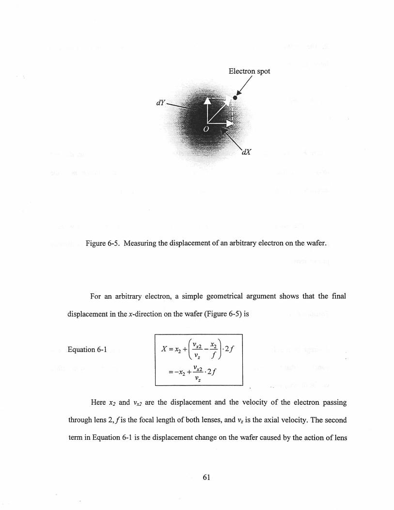
Figure 6-5. Measuring the displacement of an arbitrary electron on the wafer.
For an arbitrary electron, a simple geometrical argument shows that the final
displacement in the x-direction on the wafer (Figure 6-5) is
Equation 6-1
= -X2+ — •2/
Here X2 and Vx2 are the displacement and the velocity of the electron passing
through lens 2,/is the focal length of both lenses, and is the axial velocity. The second
term in Equation 6-1 is the displacement change on the wafer caused by the action of lens
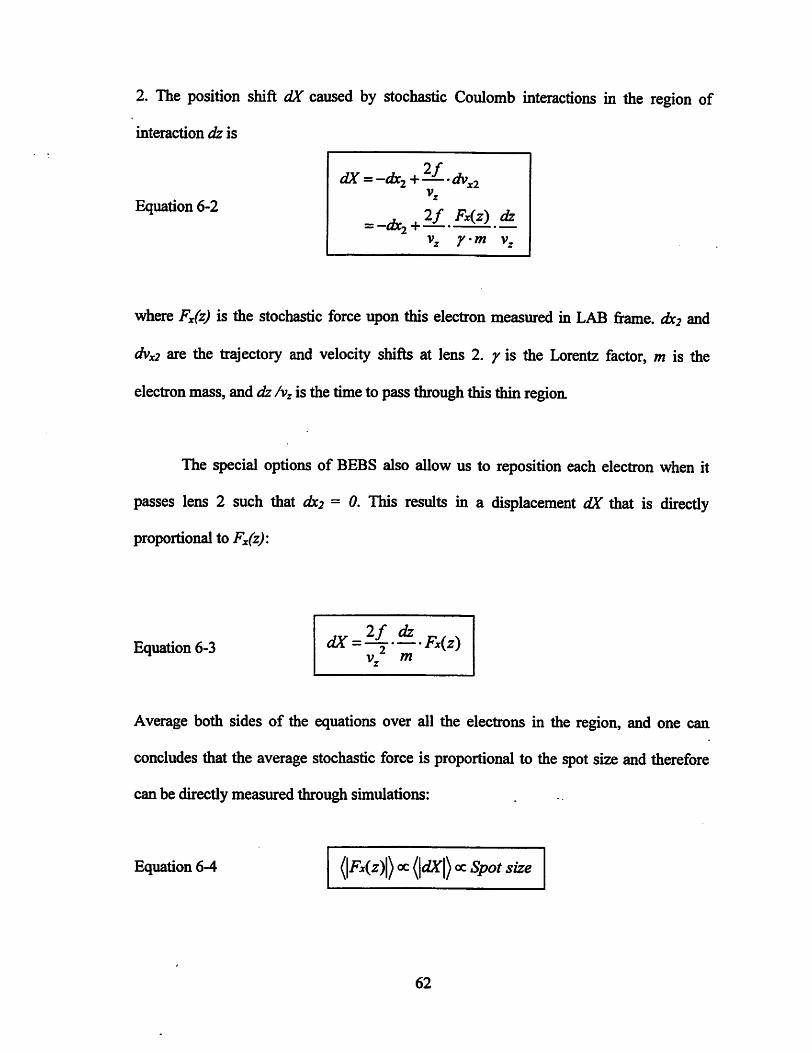
2. The position shift dX caused by stochastic Coulomb interactions in the region of
interaction dz is
Equation 6-2
dX =-dx^+^-dv,.
y-m
where Fx(z) is the stochastic force upon this electron measured in LAB frame. dx2 and
dvx2 are the trajectory and velocity shifts at lens 2. y is the Lorentz factor, m is the
electron mass,and dzhz is the timeto pass through this thin region
The special options of BEBS also allow us to reposition each electron when it
passes lens 2 such that dx2 = 0. This results in a displacement dX that is directly
proportional to Fx(z)'.
Equation 6-3
Average both sides of the equations over all the electrons in the region, and one can
concludes that the average stochastic force is proportional to the spot size and therefore
can be directly measured through simulations:
Equation 6-4 OC OC Spot size
62

The spot size is measured for each 4mm long interaction region along the beam
column. The inverse of the beam blur is plotted against the axial position z in Figure 6-6.
oo.
CO
1.2
1 o• ♦ l.U
♦ Oft♦
^ u.o
* ♦ Of;
♦
♦
U*U
ft n ii
♦ ♦
• V.Hi♦
K *%
{ • Q
•X♦
z{mm)-100 -50 50 100
Figure 6-6. Inverse of the spot size versus the axial position ofthe region of interaction.
The linear relation in Figure 6-5 indicates that spot-size(z) is inversely
proportional to z except in the region around the crossover. Thus, the average force
Equation 6-5
where the forces are still finite as the electron density is finite. Here ^ is a constant-
independent of2.
The relation in Equation 6-4 is derived for region 2. Yet, a similar argument and
result can be applied to region 1 and region 3 as long as the origin of the z-axis is moved
to the location of the emitter or the location of the wafer. The constant k, however.
63
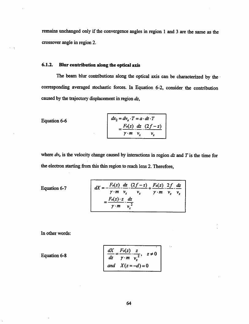
remains unchanged only if the convergence angles in region 1 and 3 are the same as the
crossover angle in region 2.
6.1.2. Blur contribution along the optical axis
The beam blur contributions along the optical axis can be characterized by the
corresponding averaged stochastic forces. In Equation 6-2, consider the contribxition
caused by the trajectory displacement in region dz.
Equation 6-6 dx2 = dVx'T = a-dt-T
_ Fx{z) dz (2f -z)y-m V,
wheredvx is the velocity change caused by interactions in regiondz and T is the time for
the electron starting from this thin regionto reach lens 2. Therefore,
Equation 6-7
In other words:
Equation 6-8
Fx(z) dz (2/-Z) ^Fx{z) 2/ dzy m Vx
_ Fx{z)'z dzym
ym Vx
dX Fx{z) z—= 2'dz y-m V/
and J!f(z= -t/) = 0
64

The boundaiy condition comes from the assumption that Coulomb interactions
only occur in the region between the two lenses where -d < z <d. Now we will prove
that
Equation 6-9I) _ <|f^(z)i)
dz m vzz
Figure 6-3 shows that Fx(z) only changes its sign at the crossover where z=0.
Therefore the proof can be shown in two separate cases.
65
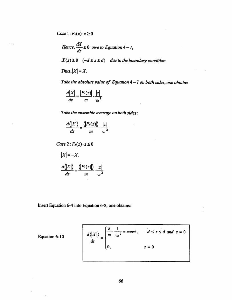
Case 1: Fx(z) •z > 0
(DCHence, — >0 owe to Equation A-1,
ck
X(z)>0 (-d <z<d) due to the boundary condition.
Thus,\X\ =X.
Take the absolute value of Equation A-1 on both sides, one obtains
d\x\ |Fx(z)| |z|<h m vz^
Take the ensemble average on both sides:
d{\X\) (|Fx(z)|) |z|dz m vz^
Case 2: Fx{z) •z < 0
|jr|=-x.
^(|X|) (|F.(z)|)dz m vz
Insert Equation 6-4 into Equation 6-8, one obtains:
Equation 6-10
r k 1z- = const,
m Vz-d < z ^ d and z ^ 0
dz
[o. z = 0
66
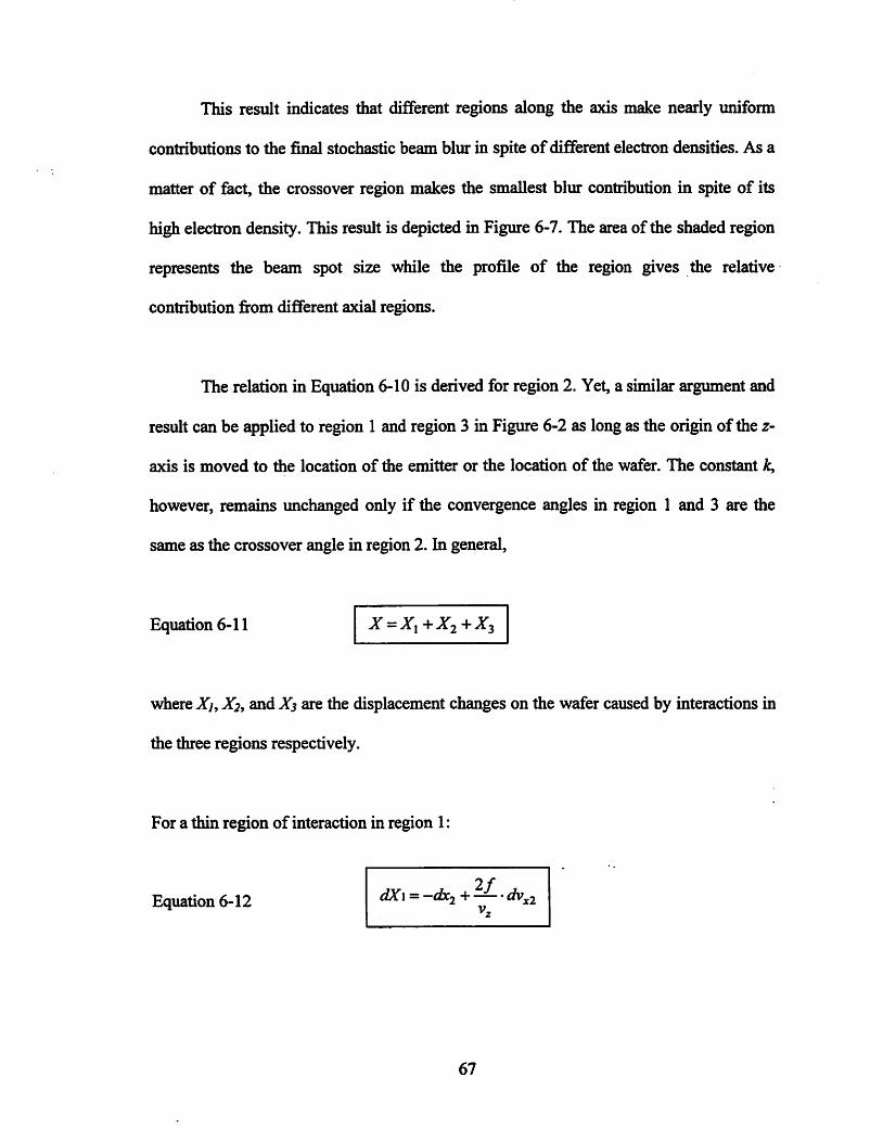
This result indicates that different regions along the axis make nearly uniform
contributions to the final stochastic beam blur in spite ofdifferent electron densities. As a
matter of fact, the crossover region makes the smallest blur contribution in spite of its
high electron density. This result is depicted in Figure 6-7. The area of the shaded region
represents the beam spot size while the profile of the region gives the relative
contribution from different axial regions.
The relation in Equation 6-10 is derived for region 2. Yet, a similar argument and
result can be applied to region 1 and region 3 in Figure 6-2 as long as the origin of the z-
axis is moved to the location of the emitter or the location of the wafer. The constant
however, remains unchanged only if the convergence angles in region 1 and 3 are the
same as the crossover angle in region 2. In general.
Equation 6-11
where Xj, X2, and X3 are the displacement changes on the wafer caused by interactions in
the three regions respectively.
For a thin region of interaction in region 1:
Equation 6-12 dX\ = -dX', + •dv
67

where dx2 and dvx2 are still the displacement and velocity changes at lens 2 but they are
caused by interactions in dz oi region 1 instead of region 2. Simple geometrical
arguments show that:
Equation 6-13
4fdx2 =-3d5cj
where dxj and dvxi are the displacement and the velocity changes at lens 1 due to the
interactions in thin region dz . Substitute Equation 6-13 into Equation 6-12, and one
obtains:
dX\ = -{r^dx^ + ^xi)+—
Equation 6-14
Using the same argument as the one used in the derivation of Equation 6-10, it can be
shown that
Equation 6-15 7 = const, -2d<z<-dm V
68

In the above derivation, we have used the fact that k remains the same for region 1 as it
shares the same beam angle as region 2. Similarly,
Equation 6-16 rf(iX3|) _^ 1 ^2 ~consty a <2 <2d
z = 2d
The differential blur contributions in all three regions are depicted in Figure 6-7. Notice
that the regions near the electron source or the wafer make little blur contribution similar
to the crossover region.
Beam with a crossover
Homocentric parallel beam
/
Figure 6-7. Beam-blur contributions along the optical axis for a crossover beam and a
homocentric parallel beam that share the same beam angle.
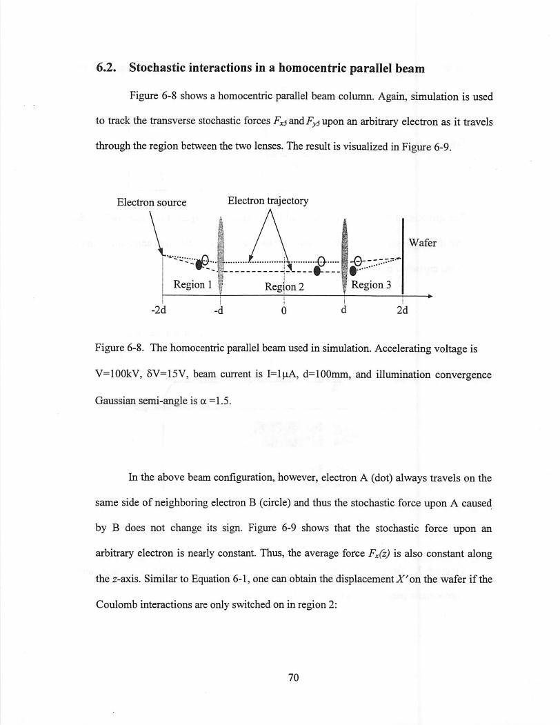
6.2. Stochastic interactions in a homocentric parallel beam
Figure 6-8 shows a homocentric parallel beam column. Again, simulation is used
to track the transverse stochastic forces Fxs andFys upon an arbitrary electron as it travels
through the region between the two lenses. Theresult is visualized in Figure 6-9.
Electron source
Region 1
Electron trajectory
k Q1^—
Region 2 Region 3
Wafer
Figure 6-8. The homocentric parallel beamused in simulation. Accelerating voltage is
V=100kV, 6V=15V, beam current is I=l|aA, d=100mm, and illumination convergence
Gaussian semi-angle is a =1.5.
In the above beam configuration, however, electron A (dot) always travels on the
same side of neighboring electron B (circle) and thus the stochastic force upon A caused
by B does not change its sign. Figure 6-9 shows that the stochastic force upon an
arbitrary electron is nearly constant. Thus, the average force Fx(z) is also constant along
the 2-axis. Similar to Equation 6-1, one can obtain the displacement X'on the wafer if the
Coulomb interactions are only switched on in region 2:

Equation 6-17 r =:c2+f^\
^2
f)•f
=Zx2./Vz
-0.05 0.05
Figure 6-9. Stochastic forces upon an arbitrary electron as it travels through region 2. The
forces are computed with the five nearest neighboring electrons.
Analogously to the derivation ofEquation 6-7 and Equation 6-8, one obtains
Equation 6-18
Equation 6-19/_
~ = consU -d^z<ddz y-m V.
71

The analysis of region 1 and 3 are similar to that of the crossover beam and the
expressions are the sameas Equation 6-15andEquation 6-16. Thus, the blurcontribution
is nearlyuniform except in the regions near the electron source and the wafer. It can be
shown that this constant is the same as the constant in the crossover beam as long as the
two configurations share the same beam angle. The result is visualized inFigure 6-7.
6.3. Other probe forming beam configurations
The model used in the above analysis can be applied to other probe-forming
beams as well. As an example, this model predicts that the three beam columns inFigure
6-10 produce the same beam blur as long as the beam angle a remains constant. The
distance between the two lenses is always L/2 2&2i result of constant beam angle. This
prediction has been confirmed with simulations. The blur is42nm atbeam current 7=1^.
Figure 6-10. Threebeamconfigurations withthe samecolumnlength andthe same
beamangle. V=100 kV, SV=15V, L=400mm, andGaussian semi-angle a =1.5.
12
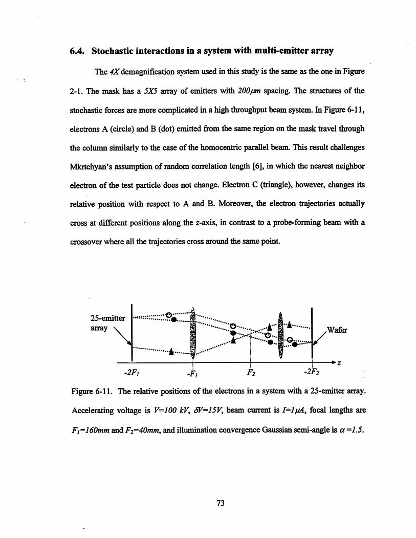
6.4. Stochastic interactions in a system with multi-emitter array
The 4Xdemagnification system used in this study is the same as the one in Figure
2-1. The mask has a 5X5 array of emitters with 200pan spacing. The structures of the
stochastic forces are more complicated in a high throughput beam system. In Figure 6-11,
electrons A (circle) and B (dot) emitted from the same region on the mask travel through
the column similarly to the case of the homocentric parallel beam. This result challenges
Mkrtchyan's assumption of random correlation length [6], in which the nearest neighbor
electron of the test particle does not change. Electron C (triangle), however, changes its
relative position with respect to A and B. Moreover, the electron trajectories actually
cross at different positions along the z-axis, in contrast to a probe-forming beam with a
crossover where all the trajectories cross around the same point.
25-emitter
array
kk
.....a-1 ir i »..j
Wafer
/
73
!
'2Fi .Fi F2 -2F2
Figure 6-11. The relative positions of the electrons in a system with a 25-emitter array.
Accelerating voltage is V=100 kV, 5F=15V, beam current is I-lpiA, focal lengths are
F 1=160mm and F2=40mm, and illumination convergence Gaussian semi-angle is a =1.5.
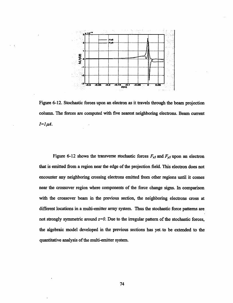
£•0mT
£
: 1
1 1
FxS
Fyfr
j
_ ^ 1
X ii f
L t i
1i
1
i 1
1 :t :
X 1 f i1 i /j
/ i1 t
1 \X X
! 11 x
1
ii
1X
1 1
1 :[t
1-OA -OAS -OA -0.1a -0.1 -OAS
Figure 6-12. Stochastic forces upon an electron as it travels through the beam projection
column. The forces are computed with five nearest neighboring electrons. Beam current
1=1^.
Figure 6-12 shows the transverse stochastic forces and upon an electron
that is emitted fi-om a region near the edge of the projection field. This electron does not
encounter any neighboring crossing electrons emitted firom other regions until it comes
near the crossover region where components of the force change signs. In comparison
with the crossover beam in the previous section, the neighboring electrons cross at
different locations in a multi-emitter array system. Thus the stochastic force patterns are
not strongly symmetric around z=0. Due to the irregular pattern of the stochastic forces,
the algebraic model developed in the previous sections has yet to be extended to the
quantitative analysis ofthe multi-emitter system.
74

6.5. Conclusions
The structures of stochastic Coulomb interactions have been revealed both in
probe-forming beams and in multi-spot projection electron beam columns. A technique
combiningan algebraic approach and simulations has been developedfor the analysis and
comparison of the stochastic Coulomb interactions and the stochastic blur. It has been
shown that in a crossover configuration where the beam angles are equal, the blur
yr
contribution is nearly constant along the column, very sunilar to a parallel beam. The
randomized correlation length assumption of Mkrtchyan's Nearest Neighbor Theory
needs modification to include symmetry around the crossover. The simulation shows that
the randomized correlation length is a function of the beam diameter and that correlated
interactions occur at other axial positions due to symmetry with respect to the beam
crossover. Further study is needed to investigate the possibility of reducing the stochastic
blur through manipulating its rich structures.
75
7 Scaling Laws of Stochastic Coulomb Interactions
7.0. Introduction
The previous chapter presented a combined approach to study the beam blur
contribution along the optical axis. Nevertheless, this method is no longer applicable if
one wants to rescale an electron beam system and compare the blur sizes. In contrast to
the space charge effect, the theoretical analysis of the stochastic effect is much more
sophisticated. Different theoretical models have been developed to predict the beam blur
caused by the electron-electron stochastic interactions in various beam configurations.
These theories, which are briefly introduced in Chapter 2, are based on a series of
unverified assumptions or approximations. Heretofore in simulation studies the stochastic
blur contributions have always been convolved with those of the space charge and can
only be isolated through approximation. This section describes a stochastic effect
simulator that directly measures the stochastic blur.
Figure 7-1 shows the schematic diagram of the stochastic effect simulator. BEBS
use moving positrons to eliminate the space blurs. A positron has the same mass but
opposite charge as an electron. In the simulation, the positrons in the column share the
76
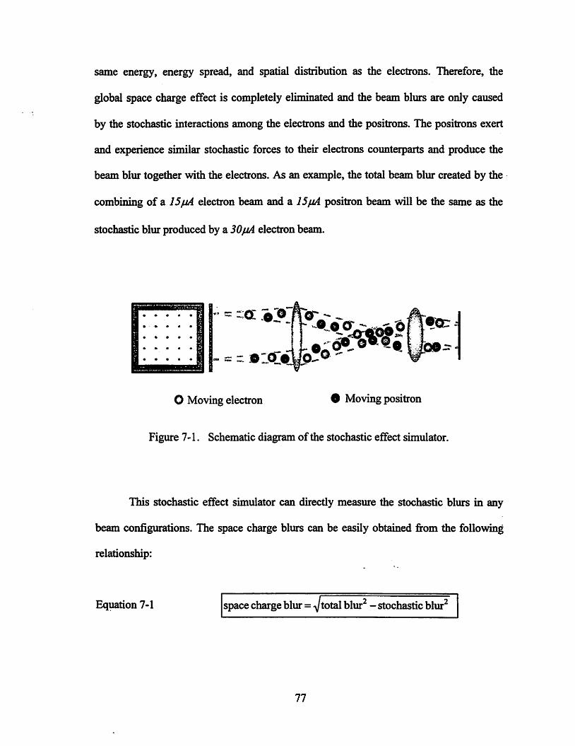
same energy, energy spread, and spatial distribution as the electrons. Therefore, the
global space charge effect is completely eliminated and the beam blurs are only caused
by the stochastic interactions among the electrons and the positrons. The positrons exert
and experience similar stochastic forces to their electrons counterparts and produce the
beam blur together with the electrons. As an example, the total beam blur created by the
combining of a ISfjA electron beam and a 15fjA positron beam will be the same as the
stochastic blur produced by a SO^A electron beam.
- =r zCSL .o"®
O Moving electron 9 Moving positron
Figure 7-1. Schematic diagram of the stochastic effect simulator.
This stochastic effect simulator can directly measure the stochastic blurs in any
beam configurations. The space charge blurs can be easily obtained from the following
relationship:
Equation 7-1 space charge blur =-Jtotal blur^ - stochastic blur^
77

7.1. Theory
This section provides a preliminary proof of the validity of the stochastic effect
simulator. Figure 7-2 shows the cross sections of two identical beam columns A and B,
one for an ordinary electron beam simulator and the other for the corresponding
stochastic effect simulator. Assume that the particle locations in either of the columns
follow identical and independent distributions. Two test electrons are at identical
positions of the two columns as shown in the figure. Fx, Fy, F*x and F*y are the total
forces upon them caused by other electrons in the column. Now we claim:
Equation 7-2 Vanance{F^)=Variance{Fj^)
Equation 7-3 Variance{Fy)=Variance[Fy)
Without losing generality, it is sufficient to show:
Equation 7-4 e{f^)-E^{F)= e{f^)
Remember that £^Fj=0 due to the effect of positrons. HereF =^FJ, F =^^Ff,/=! /=1
where F) and F^ are the forces caused by particle i in the respective columns. Moreover,
all the FjS follow the same statistical distribution, i.e., /(f;)=/{Fj), /(^)=/(^) if
particles iis positive and/(- Ff)= /{Fj) ifparticles iis negative.
In order to show Equation 7-4, we first show
Equation 7-5 e{(F, +F^f)- +F2)= +fJI
78

where particle 1 and 2 carry oppositecharges in the stochastic effect simulator column B.
LHS =e{f^ + +2• •Fj)- E^{Fi)-E^{F2)-2•E{Fi)-^(Fj)=2-Far(F,)
RHS =f((F, - F2)')= f(f,' +Fj^ - 2•F, •F2)
=f(f,')+ f(f2')- 2•F{F,)- E(F2)- F'(F,)- E^{F2)+ £'(F,)+ £'(Fj)=2Far(F|)
= LHS
Now, all the particles with opposite charges in column B can be paired. Similarly, all the
electrons in column A are also paired. Each pair ofparticles produces a total force, which
conforms to similar independent distribution in two columns. Analogous to the derivation
ofEquation 7-5, it can be shown that E^{f)= N•Var{Fi)=
Remember that the position of the test electron in each coluirm is arbitrary. The
variance of the force is actually a good measurement of the magnitude of the stochastic
force. Hence, the stochastic forces at identical positions in the two columns are roughly
equal. Therefore, the stochastic effect simulator produces the same stochastic blur as the
original electron beam column.
79
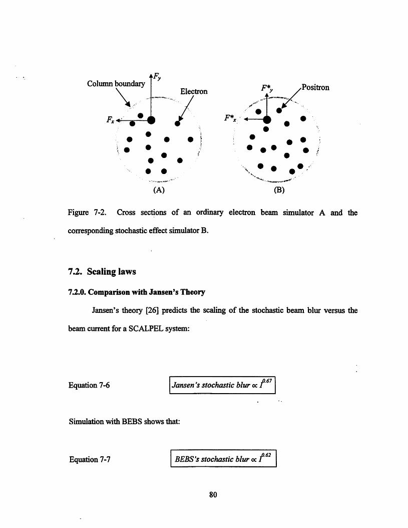
Column boundaryElectron
F* .Positron
F*X
(A) (B)
Figure 7-2. Cross sections of an ordinary electron beam simulator A and the
corresponding stochastic effect simulator B.
7.2. Scaling laws
7.2.0. Comparison with Jansen's Theory
Jansen's theory [26] predicts the scaling of the stochastic beam blur versus the
beam current for a SCALPEL system:
Equation 7-6 Jansen'sstochastic blur oc f
Simulation with BEES shows that:
Equation 7-7 BEBS's stochastic blur oc f
80

The simulation results roughly agree with Jansen's prediction. Nevertheless, the
spot size is larger than Jansen's prediction at each current as shown in Figure 7-3. Jansen
made a series of approximations and assumptions, which includes: (1) each electron only
being involved in one or no strong collisions in a beam segment, and (2) the interactions
being fully correlated in one beam segment and fully uncorrelated between beam
segments. These approximations all contribute to the above discrepancy.
SCALPEL
Jansen^s analysis
l^tA)
' t I
10.1 12.1 14.1
Figure 7-3. Comparison between the stochastic blur measured with BEBS and the blur
from Jansen's prediction.
7.2.1. Scaling laws for a 25-emitter array system
The applications of Jansen's theoretical model are restricted by the beam
configurations due to its complexity. The stochastic effect simulator, however, can be
81
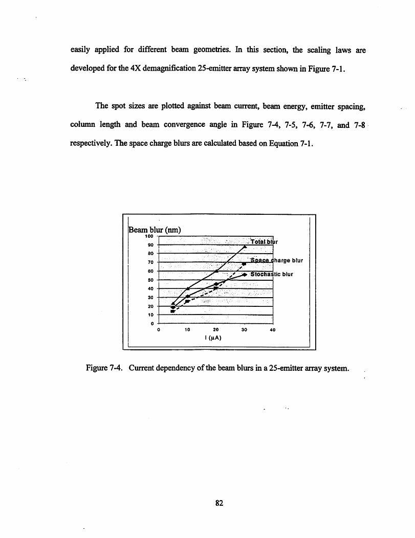
easily applied for different beam geometries. In this section, the scaling laws are
developed for the 4X demagnification 25-emitter arraysystem shown in Figure 7-1.
The spot sizes are plotted against beam current, beam energy, emitter spacing,
column length and beam convergence angle in Figure 7-4, 7-5, 7-6, 7-7, and 7-8
respectively. The space charge blurs are calculated based on Equation 7-1.
Beam blur (nm)100 T
I(mA)
Total bl ur
Spflgft fjhargft blur
Stocha! tic blur
Figure 7-4. Current dependency ofthe beam blurs in a 25-emitter array system.
82

i Beam blur (nm)! 120
300E(keV)
Figure 7-5. Beam energy dependency ofthe stochastic blur and the space charge blur.
Beam blur (nm)
80
70
I 60I 50i 40I 30
20
I 10
i 0
^ charge blig
Stochastichlur
02 0.3 0.4 0.5
Emitter spacing (pm)0.6
Figure 7-6. Emitter spacing dependency ofthe stochastic blur and the space charge blur.
83
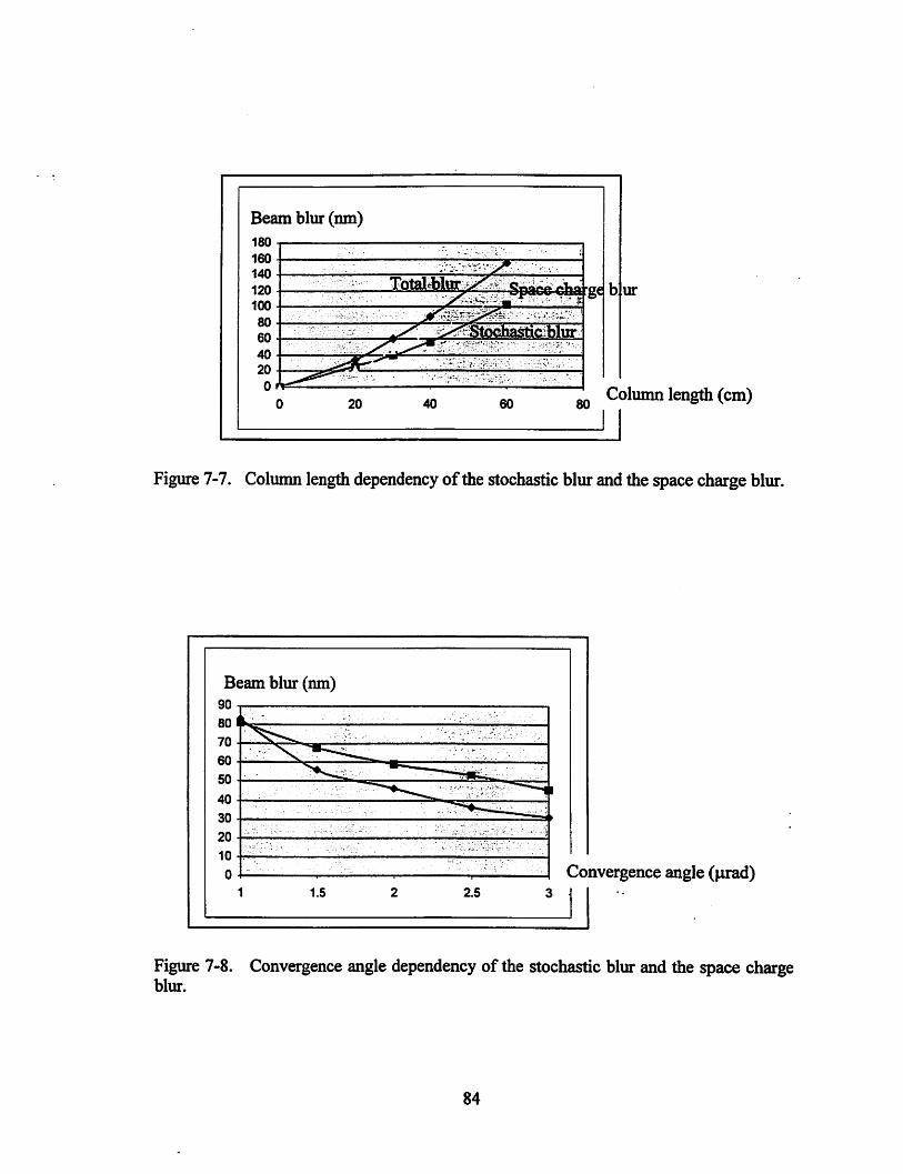
Beam blur (mn)180
180
140
120
100
80
60
40
20
0
20
Totaleblur
40
Space elm :ge ur
60 80Column length (cm)
Figure 7-7. Column length dependency ofthe stochastic blur and the spacecharge blur.
Beam blur (nm)
Convergence angle (prad)
Figure 7-8. Convergence angle dependency of the stochastic blur and the space chargeblur.
84
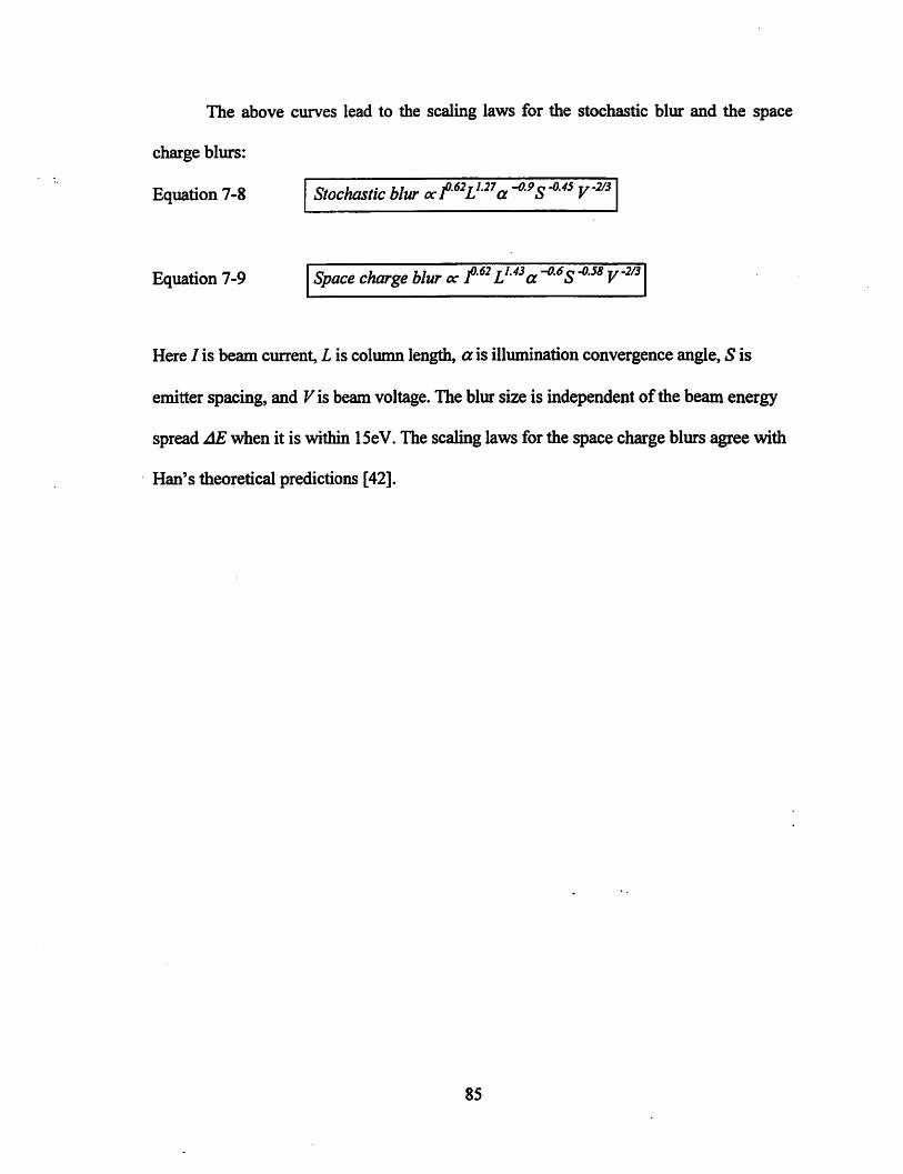
The above curves lead to the scaling laws for the stochastic blur and the space
charge blurs:
Equation 7-8 Stochastic blur ccfH'^a -"'S V"'
Equation 7-9 Space charge blur oc f
Here I is beam current, L is column length, a is illumination convergence angle, S is
emitter spacing, and Vis beamvoltage.The blur size is independent ofthe beam energy
spread AE when it is within 15eV.The scaling laws for the space charge blurs agree with
Han's theoretical predictions [42].
85
8 Impact ofPositive Ions and Effect ofLens
Aberrations
8.0. Introduction
The aberrations induced by the lensing action of global space charge of the
electrons result in beam blur that increases with beam current, as first demonstrated by
Han et al [3]. There are a lot of papers which deal with space charge neutralizations in
various systems such as cathode ray tube (CRT) and focused ion beams [45] [47].
However, it is not clear whether the neutralization scheme would be effective for the high
throughput e-beam due to the light mass of electrons. Xiu [30] [31] studied the effect of
space charge coils and a multi-pole projector in electron beam columns and tried to
reduce field curvature and on-axis aberrations. Nevertheless, no quantitative results have
been given on the beam blur reductions. This chapter discusses techniques that
effectively reduce the space charge effect Section 8.1 investigates the feasibility of
reducing the global space charge with stationary neutralizing ions in electron beam
columns. Section 8.2 explores the feasibility of reducing space charge effect with induced
lens aberration. The summary and conclusions are given in Section 8.3.
86

8.1. Impact of positive ions
The beam blur produced in an electron beam system can be decomposed into
stochastic blur and space charge blur, which are caused respectively by the stochastic
Coulomb interactions and the global space charge effect. Introducing a cloud of positive
ions in the electron beam column can reduce the global net charge and thus decrease
space charge blur. However, this will cause a considerable increase in stochastic blur
contribution due to the increased opportunity for collisions. Changes of the total beam
blur depend on the trade-off between these two competing tendencies. The schematic
diagram is shown in Figure 8-1.
Total beam blur
tStochastic beam blur Space charge blur
Electron - electron
interactions.
tElectron-ion I I Ion spaceinteractions. I I charge
lonization state
Electron spacecharge
Figure 8-1. Effect ofneutralizing ions upon electron beam blurs.
87

Figure 8-2 shows the simulated multi-emitter array system with both projection
electrons and positive ions in the column. The ions are assumed to be stationary
compared to fast moving electrons because of their large masses. To find the most
favorable configuration, ion distributionA and distribution B are tested. In configuration
the relation between the ion number densities and the electron number densities are
given by:
Equation8-1 fix,y,z) -f^,y,z)ly
throughout the beam column. The space charge effect is completely eliminated in this
case, y is caused by the relativistic effect. In configuration 5, however, ions are
introduced only in the region between the two lenses where their distributions follow
Equation 1. The space charge effect is partially eliminated here. In our initial studies,
each ion is assumed to have only one positive charge (such as
88
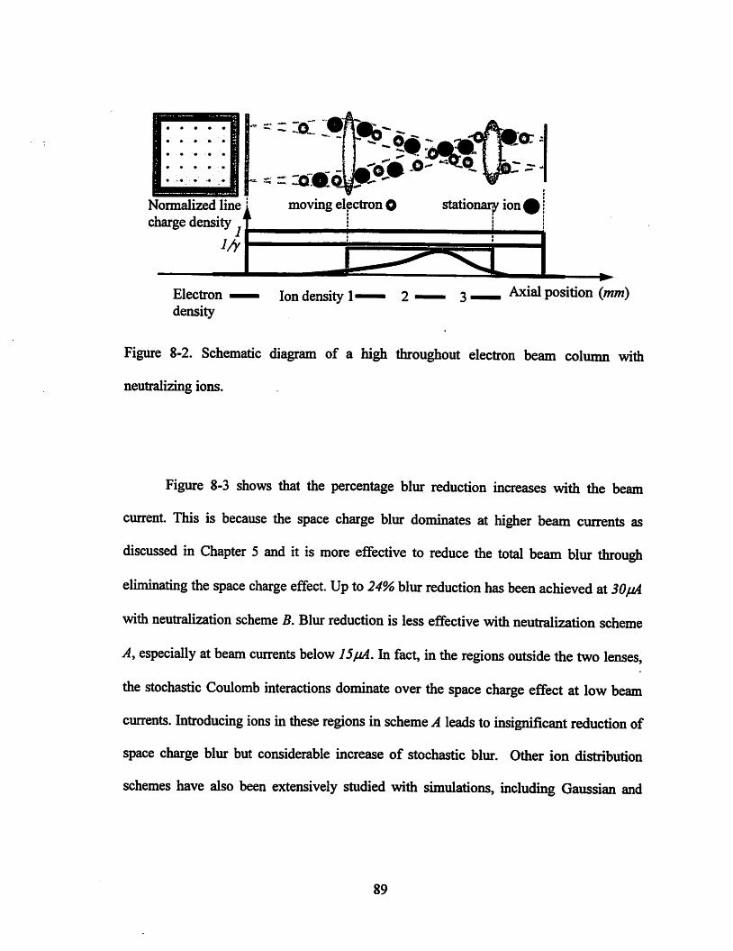
Nonnalized line 1
charge density
Electron
density
- ZQl J
moving electron O
Ion density 1'
stationaiy ioni
Axial position (mm)
Figure 8-2. Schematic diagram of a high throughout electron beam column with
neutralizing ions.
Figure 8-3 shows that the percentage blur reduction increases with the beam
current. This is because the space charge blur dominates at higher beam currents as
discussed in Chapter 5 and it is more effective to reduce the total beam blur through
eliminating the space charge effect. Up to 24% blur reduction has been achieved atSOjuA
with neutralization scheme B. Blur reduction is less effective with neutralization scheme
A, especially at beam currents below I5juA. In fact, in the regions outside the two lenses,
the stochastic Coulomb interactions dominate over the space charge effect at low beam
currents. Introducing ions in these regions in scheme A leads to insignificant reduction of
space charge blur but considerable increase of stochastic blur. Other ion distribution
schemes have also been extensively studied with simulations, including Gaussian and
89

Lorentzian distributions along the optical axis. Scheme B gives the best blur reduction
found to date.
100
90
80
70
E'S 500)
•S 40
1ST20
10
0
25 EmitterArr^
•^no neutralization
'neutralizationtlirough out thecolumn
>neutralization only inthe region betweenthe tMO lenses
Figure 8-3. Beam current dependency of spot sizes for differentneutralization schemes.
Figure 8-4 shows the point spreads on the optimal target plane without
neutralizing ions (left) and with neutralization scheme B (right). With the presence of
ions, the beam spots near the edge of the field are smaller and much more symmetric.
Some residual aberration still appears to be present in the image on the right because only
electrons in the region between the lenses are neutralized.
90
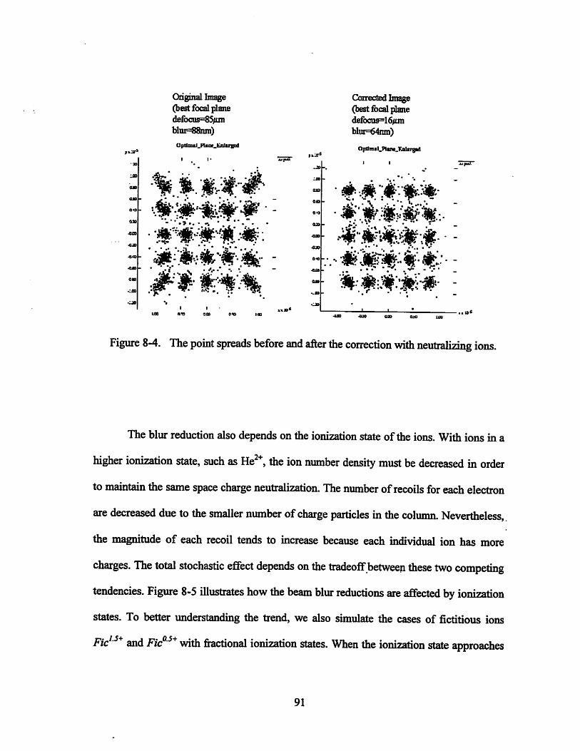
*»
OJO
OiO
040
oao
•om
•a»
on
'.CO
Qdginal Image(best focalplanedefi>cu8=€S/un1diu=SSnm)
OptliBftl.Ksar.E&IuieccI
t I
Ltt 0*0 on on loa
CU0
on -
0*0
0l2» -
•on -
•on
on -'
nn -
on -
-.00 -
CorrectedImage(bestfocalplanedefociiSF=16^blm=64nm)
Opdmal.PteM.Kaltrgid
•UD •OHO QOO QsO UXI•*»(
Figure 8-4. The point spreads before and after the correction with neutralizing ions.
The blur reductionalso depends on the ionization state of the ions. With ions in a
higher ionization state, such as He^^, the ion number density must be decreased in order
to maintainthe same spacecharge neutralization. The numberof recoils for each electron
are decreased due to the smaller number of charge particles in the column. Nevertheless,
the magnitude of each recoil tends to increase because each individual ion has more
charges. The total stochastic effect depends on the tradeoff between these two competing
tendencies. Figure 8-5 illustrates how the beam blur reductions are affected by ionization
states. To better understanding the trend, we also simulate the cases of fictitious ions
and with fractional ionization states. When the ionization state approaches
91
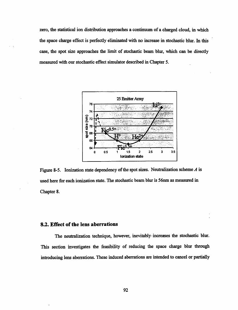
zero, the statistical ion distribution approaches a continuum ofa charged cloud, in which
the space charge effect is perfectly eliminated with no increase in stochastic blur. In this
case, the spot size approaches the limit of stochastic beam blur, which can be directly
measured with our stochastic effect simulator described in Chapter 5.
25 Emitter Array
1 1.5 2 2.5
lonization state
Figure 8-5. lonization state dependency ofthespot sizes. Neutralization scheme A is
used here for each ionization state. The stochastic beam blur is 56nm as measured in
Chapter 8.
8.2. Effect of the lens aberrations
The neutralization technique, however, inevitably increases the stochastic blur.
This section investigates the feasibility of reducing the space charge blur through
introducing lens aberrations. These induced aberrations are intended to cancelor partially
92
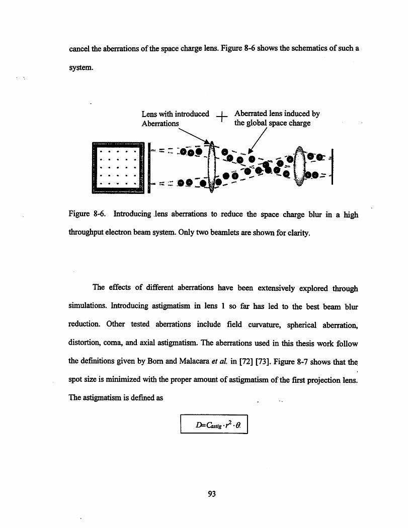
cancelthe aberrations of the spacechargelens. Figure 8-6 shows the schematicsofsuch a
system.
Lens with introduced _[_ Aberrated lens induced byAberrations the global space charge
09
A A "Af w 0r^ A wf- %
Figure 8-6. Introducing lens aberrations to reduce the space charge blur in a high
throughput electron beam system. Only two beamlets are shownfor clarity.
The effects of different aberrations have been extensively explored through
simulations. Introducing astigmatism in lens 1 so far has led to the best beam blur
reduction. Other tested aberrations include field curvature, spherical aberration,
distortion, coma, and axial astigmatism. The aberrations used in this thesis work follow
the definitions given by Bom and Malacara et al. in [72] [73]. Figure 8-7 shows that the
spot sizeis minimized withthe properamount of astigmatism of the first projection lens.
The astigmatism is defined as
I^Castig't^ '0.
93

where r is the radial distance measured on the first projection lens, ^is the incident angle
ofthe electron on the lens, and D is the corresponding position change on the target plane
caused by the aberration.
25 EmittErArr^, I=30/tA
Total Wurte
-V •
Stochastic blur size
66 132 198 264 330 396
Figure 8-7. Beam blur reduction depends on the magnitude ofthe induced astigmatism.
The beam spot reaches its minimum of61nm with 330m"^ astigmatism in the first
lens. The percentage blur reduction is about 31%. The spot size increases when the
astigmatism caused by the space charge effect is either under-compensated or
overcompensated. As one can see, the reduced beam blur closely approaches the
stochastic blur limit, which is around 56nm. Figure 8-8 shows the point spreads at the
best focal plane before and after the correction. The spots near the edge of the field are
significantly improved. Similar to neutralizing ions, the blur reduction technique with
lens aberrations is more effective at higher beam currents when the space charge blur
dominates.
94
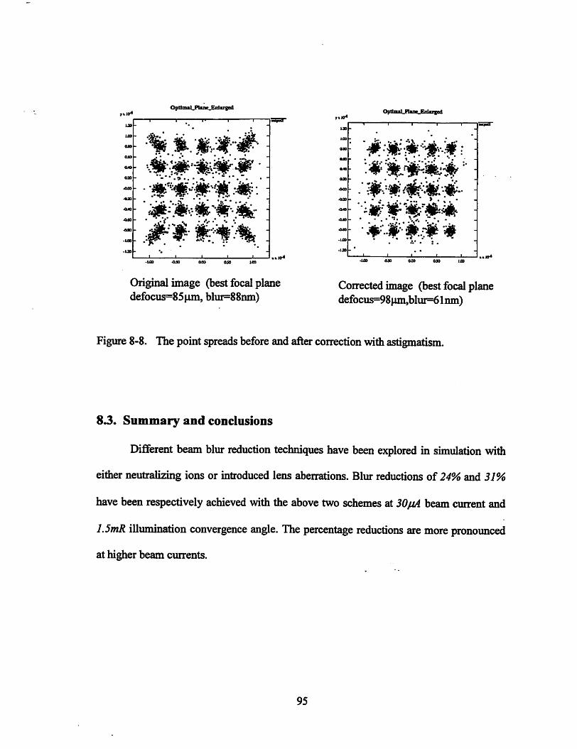
OIO
CM
CM
CM
•OflO
-CM
OptimmLPUneJBnlix^ed
OjOO 4l30 on 050 JjQO
Original image (best focal planedefocus=85pm, bliii=88nm)
f *10^
cm
aao
mac
mm
OptizBaLFUncLEnUriBed
I r 1 1 1—
.:'$•• MM ¥• •%•<•• •
•ue 4M oas «» iffl
Correctedimage (best focal planedefociis=98pm,blur=61nm)
Figure 8-8. The point spreads before and after correction withastigmatism.
8.3. Summary and conclusions
Different beam blur reduction techniques have been explored in simulation with
either neutralizing ions or introduced lens aberrations. Blur reductions of 24% and 31%
have been respectively achieved with the above two schemes at SOfiA beam current and
L5mR illumination convergence angle. The percentage reductions are more pronounced
at higher beam currents.
95
9 Electron Interaction with Photo-resist
9.0. Introduction
Since 1960s a series of Monte Carlo models have been proposed and refined to
examine the electron interactions with solids. Among these models, the hybrid model was
developed by Murata et al [22] to simulate the electron energy deposition in the photo
resist. The hybrid, however, is based on the unverified assumption that all forms of
deposited energy contribute equallyto the exposure events. The detailed mechanisms of
exposure reactions are beyondthe scope ofthis model.
The analytical Electron-Resist Interaction Model (BRIM) developed at UC
Berkeley is a recommended approach to studythe details of the electron-resist interaction
process through reaction cross sections. Section 9.1 gives the schematics of the BRIM.
Section 9.2 discusses the secondary electron emission process. Section 9.3 investigates
the exposure process using the reaction cross-sectionapproach. All of the components are
linked together in Section 9.4 and the algebraic expression describing the spatial
distribution ofthe exposure events is presented.
96

9.1. Schematics of ERIM
Figure 9-1 shows the schematic diagram of the ERIM model. The high-energy
primary electrons are emitted from a point source. Low energy secondary electrons are
emitted along the primary electron path and cause most of the exposure events, as will be
discussed in later sections. The deflection process of primary electrons caused by elastic
scattering can be separated from the secondary electron emission process for the purpose
ofanalysis.
Primary election pdnt source (lOOKeV) Photo-resist\ Exposure event
Lowenergy secondary electron(<400eV)
I
9
^ 1O-
' /1.^ / ^ ^
Real physicd Piimaiy election Secondaiy electrons productionpK)c®SB deflection andresisterqxisures
Figure 9-1. Schematic diagram of the secondary electron productions and the exposure
process.
97
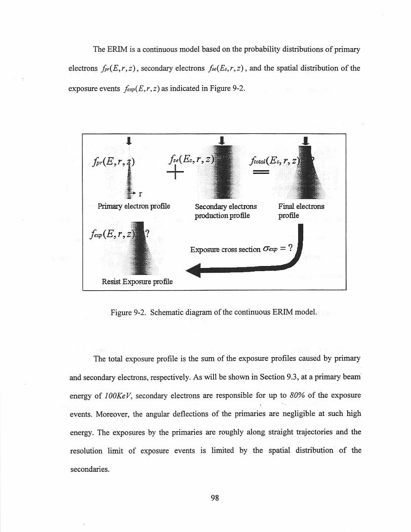
The ERIM is a continuous model based on the probability distributions of primary
electrons fpr{E^r,z), secondary electrons fse{Es^r^z), and the spatial distribution of the
exposure events fexp{E^r,z) as indicated in Figure 9-2.
fpr(E,r,s) r, z ftotai{Es, r, z
Primary electron profile
Resist Exposure profile
Secondary elections Final electionsproduction profile profile
Exposure cross section Oop —?
Figure 9-2. Schematicdiagram ofthe continuous BRIM model.
The total exposure profile is the sum of the exposure profiles caused by primary
and secondaryelectrons, respectively. As will be shown in Section 9.3, at a primary beam
energy of lOOKeV, secondary electrons are responsible for up to 80% of the exposure
events. Moreover, the angular deflections of the primaries are negligible at such high
energy. The exposures by the primaries are roughly along straight trajectories and the
resolution limit of exposure events is limited by the spatial distribution of the
secondaries.
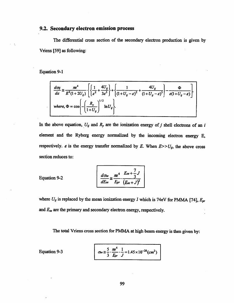
9.2. Secondary electron emission process
The differential cross section of the secondary electron production is given by
Vriens [59] as following:
Equation 9-1
day ^ 1 417, 4C/. O
+ (i+Uy-sYj e(\+U,j-€)
^ pwhere, <S> = cos \nU,
In the above equation, Uy and Ry are the ionization energy ofj shell electrons of an /
element and the Ryberg energy normalized by the incoming electron energy E,
respectively. € is the energy transfer normalized by E. When E»Uij, the above cross
section reduces to:
Equation 9-2dEse Epr (Ese-^-jy
where Uy is replaced by the mean ionization energy J which is 74eV for PMMA [74], Epr
and Ese are the primary and secondary electron energy,respectively.
Thetotal Vrienscrosssection forPMMA at highbeamenergy is thengivenby:
Equation 9-3 o&e =—• •—=1.45 X10"^®(cw^)3 Epr J
99
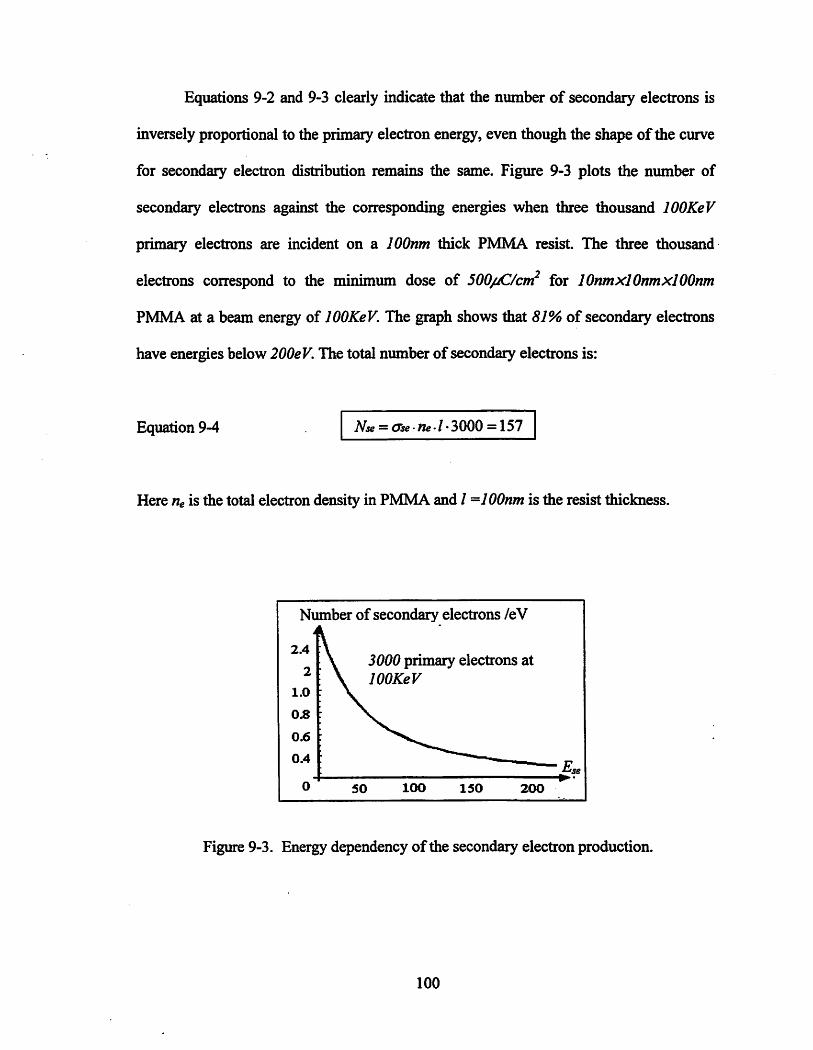
Equations 9-2 and 9-3 clearly indicate that the number of secondary electrons is
inversely proportional to the primary electron energy, even though the shape of the curve
for secondary electron distribution remains the same. Figure 9-3 plots the number of
secondary electrons against the corresponding energies when three thousand lOOKeV
primary electrons are incident on a lOOnm thick PMMA resist. The three thousand
electrons correspond to the minimum dose of 500//C/cm^ for lOnmxlOnmxlOOnm
PMMA at a beam energy of lOOKeV. The graph shows that 81% of secondary electrons
have energies below 200eV. The total number of secondary electrons is:
Equation 9-4 Nse = asene'l' 3000 = 157
Here rie is the total electron density in PMMA and 1 =100nm is the resist thickness.
Number ofsecondary electrons /eV
3000 primary electrons atlOOKeV
Figure 9-3. Energy dependency ofthe secondary electron production.
100

The number of further cascade electrons is less than ten. This number has been
evaluated using the secondary electrons at energies of 400eV or less. The effect of the
cascade electrons is not considered in later discussions due to their small number.
The modified Bethe formula by Joy and Luo [60] is used to describe the energy
loss of the secondaries along their paths:
Equation 9-5 -785-^.Inds EA
1.166(£ + 0.85J)
J
where Z, A and p are the atomic number, atomic weight and density of the photo resist
respectively. Figure 9-4 shows that 90% of the secondary electrons whose energies are
below 400eVcan only travel less than 12nm in PMMA resist Meanwhile, 81% of the
secondaries whose energies are below 200eV can only travel less than 5nm. This agrees
with the experimental result that the resolution limit for lOOnm PMMA is aroimd lOnm
[75].
Es(eV)1000
lOOeV
=1000eV
Es=4.9eV''s(nm)0 10 20 30 40 60
Figure 9-4. Energy losses ofsecondaryelectronsalong
101
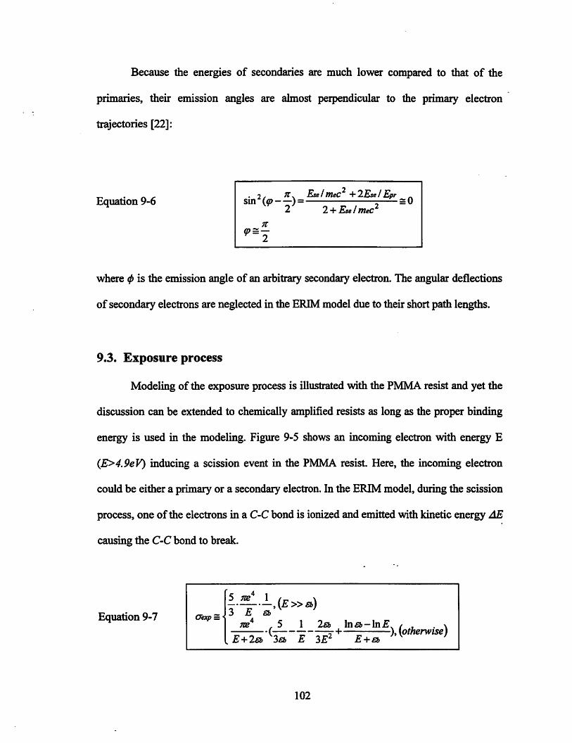
Because the energies of secondaries are much lower compared to that of the
primaries, their emission angles are almost perpendicular to the primary electron
trajectories [22]:
Equation 9-62, /T. Rse!tneC^ •\-'2.EselEpr ^
sm
TV(p = —
2
where 0 is the emission angle of an arbitrary secondary electron. The angular deflections
of secondary electrons are neglected in the ERIM model due to their short path lengths.
9.3. Exposure process
Modeling of the exposure process is illustrated with the PMMA resist and yet the
discussion can be extended to chemically amplified resists as long as the proper binding
energy is used in the modeling. Figure 9-5 shows an incoming electron with energy E
{E>4.9eV) inducing a scission event in the PMMA resist. Here, the incoming electron
could be either a primary or a secondary electron. In the ERIM model, during the scission
process, one of the electrons in a C-C bond is ionized and emitted with kinetic energy AE
causing the C-C bond to break.
Equation 9-7 Cexp =
a)3 E £b
,5 1 2a. lna.-ln£. / , . \( 7 H ), {otherwise}
E + lsb 3£b E 3E^ E + £b ^ '
102

Since a secondary electron emission is involved, Vriens cross section is used to
calculate the scission cross section:
Equation 9-8Oexp =
—,(£»£6)3 E €b
;ie'̂ , 5 I Isb ln£&-ln£^ / , ^( 7 H ), [otherwise)
£+2a 3a. E 3E^ E + a ^ '
where €b is the C-C binding energy of 4.9eV.
E-AE- &
Figure 9-5. Schematic diagram of a scission event in PMMA.
Figure 9-6 shows how the exposure cross section changes with the electron
energy E. The cross section is maximal when the electron energy is close to the C-C bond
energy and decreases at large energies.
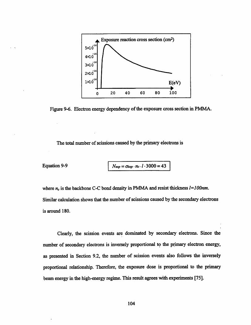
k Exposure reactioncross section (cm^)-16
5x10
-16
4x10 /-16
3X10
-16
2X10 ^—.-16
1X10 E(eV)
()
w
20 40 60 80 100
Figure 9-6. Electronenergydependency ofthe exposure cross sectionin PMMA.
The total number ofscissions caused by the primary electrons is
Equation 9-9 Nexp —Oaq) -TlC'l •3000 —43
where ric is the backbone C-C bond density in PMMA and resist thickness l=100nm.
Similar calculation shows that the number ofscissions caused by the secondary electrons
is around 180.
Clearly, the scission events are dominated by secondary electrons. Since the
number of secondary electrons is inversely proportional to the primary electron energy,
as presented in Section 9.2, the number of scission events also follows the inversely
proportional relationship. Therefore, the exposure dose is proportional to the primary
beamenergy in the high-energy regime.This result agrees with experiments[75].
104

9.4. Spatial profile of exposure events
After the detailed investigation ofsecondary electron production and exposure
mechanisms, we develop a formulation to describe the global distribution ofthe exposure
events. The number ofexposure events per unit distance along a secondary electron path
can be evaluated based on the modified Bethe formula and the exposure cross section in
the previous sections:
Equation 9-10
Ga^Ese\nb- Gex^Ese{Eso,r '̂ rib
where, Gap=m
(5 1 2a lna-ln£r
Ese 4* 2a 3a Ese 3Ese^ Ese + Sb
The number of secondary electrons emitted per unit energy is:
Equation 9-11das Tva^rie
-ru^
dEso Epr{Eso +*/)^
Combining Equation 9-9 and Equation 9-10, one obtains the spatial distributions
ofthe exposure events caused by the secondary electrons when a single primary electron
incidents on the resist:
Equation 9-12aexp\Ese{E5o, r)\ rib das
105
(8)
(9)
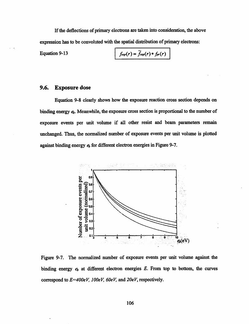
If the deflections ofprimary electrons are taken into consideration,the above
expression has to be convoluted withthe spatialdistribution of primary electrons:
Equation 9-13 I fejv{r) =fcxp{r)*fpr{r)
9.6. Exposure dose
Equation 9-8 clearly shows how the exposure reaction cross section depends on
binding energy €b. Meanwhile, the exposurecross sectionis proportional to the numberof
exposure events per unit volume if all other resist and beam parameters remain
unchanged. Thus, the normalized number of exposure events per unit volume is plotted
against binding energy €b for differentelectron energiesin Figure9-7.
iS *0 08c g
il"^ Bq£
sw GO ^^05CL, 4}
^(eV)
Figure 9-7. The normalized number of exposure events per unit volume against the
binding energy eb at different electron energies E. From top to bottom, the curves
correspond to E=400eV, lOOeV, 60eV, and 20eV,respectively.
106
As discussed in Section9.2 and Section9.3, the exposure reactions are dominated
by the secondary electrons at energies of400eVor below. Figure 9-6 shows thatat energy
E=400eV, the number of exposures perunit volume is inversely proportional to binding
energy ei, if other resist and beam parameters remain unchanged. For energy below
400eV, the number ofexposures decreases even faster. In order to maintain the minimum
number of exposures per unit volume, one must increase the exposure dose and thus
increase the numberof secondary electrons. The exposure dose follows the conventional
definition, which is the amount of charges incident on a unit area of the photo-resist.
Therefore, the ERIM model predicts that the minimal exposure dose is a super-linear
fimction of the binding energy et. Ontheother hand, a larger binding energy will leadto
smaller line width if the exposure dose is held constant. These results are beyond the
firework ofMurata's Hybrid model, which only considers total deposited energy rather
than exposure cross sections.
9.7. Conclusions and discussion
An analytical electron resist interaction model BRIM has been developed to study
the detailed mechanisms of the exposure events. It has been found that secondary
electrons are responsible for up to 80% of the exposure events. The model predicts that
the minimum exposure dose ijjC/cnf) is proportional to the primary electron energy in
the high-energy regime, which agrees with experiments. The BRIM model also predicts
that the minimal exposure dose is a super-linear fimction of the binding energy for
exposures ifother resist and beamparameters remainunchanged. This result is still to be
107
confirmed in experiments. The above results are beyond the scope of the hybrid model
developed by Murata, which only considers the total energy deposited in the resist.
An algebraic expression is derived for the spatial distribution of the exposure
events. The expression is suitable for numerical solution. The ERIM model can be
extended to chemically amplified resists by adjusting the binding energy.
There are still some open questions regarding the resist exposure process and the
BRIM model. According to the predictionofthe ERIM model, only aroimd 22.3 exposure
events occur in a lOnmxlOnmxlOnm volume of PMMA at the minimum exposure dose
of500^/cm^.The average spacing between adjacent exposures is3.5nm. For chemically
amplified resist,the minimumexposure dose is usually five times smaller and the spacing
between adjacent exposures would be around 6nm. This inhomogeneity of exposures can
be smoothed out during the post exposure bake.
Experimental results by Shultz [76] and Greeneich [77] show respectively 0.0169
scissions/eV and 0.019 scissions/eV in PMMA polymer. This number is roughly nine
times as large as the prediction by ERIM. One possible explanation for the discrepancy is.
that the ERIM model so far only includes exposure events that are directly caused by
electron interactions with the C-C bond in the main chain. As a matter of fact, primary
and secondary electrons also interact with other chemical bonds in PMMA and produce
different kinds of radicals. Shultz [76] [78], Alexander [79], and Kircher [80] suggest that
some of these radicals can rupture the main chain by disproportionation, which may
108

explain the ease of PMMA backbone rupture. There is still no consensus on the detailed
mechanisms. If all the exposures caused by the radicals were included, the total number
of exposure events would be considerably larger than the number predicted by ERIM.
Nevertheless, the basic approach of BRIM can be extended to include the effect of
radicals. The main conclusions given earlier in this section would still be valid since the
binding energies for the backbone scissionand for the radicalproductions are roughly the
same.
The accuracy of the BRIM model also depends on the accuracy of the physical
models such as the modified Bethe formula by Joy and Luo at energies below lOOeV
whenthe exposurecross section is very large. Further investigations are required in order
to explain the discrepancies and to improve the BRIM model.
109

10 Conclusions
10.0. Numerical and analytical tools
In this thesis, three simulation and analytical tools are developed to study the
electron Coulomb interactions in beam columns and electron interactions with photo
resist.
The Berkeley Electron Beam Simulator (BEBS), developed by the author, is a
software program used to simulate the electron interactions in beam columns. It employs
adaptive Fast Multipole Method and parallel codes for efficient and rigorous calculation
of Coulomb forces. It also uses continuous-force interpolation and adaptive time steps to
speed up time iteration. BEBS provides a series of options specific for studying the
mechanisms ofbeam blur production. All of these special options have been successfiilly
used to produce the academic contribution of this thesis. As one of the options, BEBS
enables the stochastic effect simulator using positrons in the beam column, which directly
produce the stochastic blur on the target plane.
110
There are two versions of BEBS running on the Network of Workstations (NOW)
and the Millennium Cluster, respectively. A typical 30pA current simulation in a 40cm
long column takes about one hourwith ten 500MHz processors. Comparedwith Munro's
electron beam simulator that has 9 to 4 percent errors in force calculation at a beam
current of 5 to 30|xA, BEBS can achieve up to 4-digit accuracy in forces with 3 to 5 times
longer simulation time.
In order to study the structure of stochastic Coulomb interactions, the author
developed a novel approach that combines simulation techniques and algebraic analysis.
It not only avoids the sophisticated algebra and approximations of a conventional
analytical approach but also reveals the structure of stochastic Coulomb interactions in
certain beam configurations. This new approach has been successfully applied to the
analysis ofa crossover configuration and a homocentric parallel beam.
The BerkeleyElectron-Resist Interaction Model (ERIM) has been investigated as
an analytical approach to study electron resist interaction mechanisms based on reaction
cross sections. This model provides an algebraic expression for the spatialdistributionof
exposure events in the photo resist.
10.1. Mechanism studies and beam blur reductions
This thesis discusses different mechanisms that cause beam blur in beam columns
and in photo-resist. Severalpotential techniques for blur reductionsare also proposed.
Ill
Studies show that beam blur is mostly produced in the region around the
crossover in a multi-emitter array system. Thus, any blur reduction technique only need
to focus on its effect on this region. Meanwhile, the blur contributions caused by inter-
beamlet electron interactions dominate over those caused by intra-beaiiilet electron
interactions, especially at large convergence angles. Effective ways are still to be foimd
to isolate and reduce the inter-beamlet blur contributions. The beam blur contributions
from different beamlets can be combined on a root mean square basis.
Mechanism that causes stochastic blur is examined from different perspectives.
Unlike the space charge blur, stochastic blurs can not be easily reduced with conventional
optics. Further studies are required in order to fully utilize the structure of stochastic
interactions for possible blur reductions.
Although the stochastic effect has long been observed, it has never been directly
measured in experiments and or in simulations. The Stochastic Effect Simulator enables
the direct measurement of stochastic blur and demonstrates the '^stochastic limif for any
technique that reduces space charge blur only. Simulations show that in 4x
demagnifrcation electron beam systems, the stochastic blur is proportional to beam
current raised to the power of 0.62, column length raised to the power of 1.27, beam
convergence angle raised to the power of -0.9, emitter spacing raised to the power of -
0.45, and beam voltage raised to the power of-2/3. The scaling exponent 0.62 for beam
current roughly agrees with Jansen's prediction of 0.67. The blur size is independent of
the beam energy spread AE when it is within ISeV. Scaling laws for space charge blurs
112

are also developed. The scaling exponents agree with Han's simulation and experimental
results [3] [42].
Simulations are used to test the basic assumptions of Mkrtchyan's theory on
electron stochastic interaction in a beam column: (1) consideration of nearest-neighbors
only, and (2) a randomized length, over which interactions are correlated. Analysis of a
basic crossover beam shows that interactions with multiple rather than nearest
neighboring electrons almost immediately become the norm rather than the exception as
proposed by Mkrtchyan. Thesimulation shows that the randomized correlation length is a
function of the beam diameter and that correlated interactions occur at other axial
positions due to symmetry with respect to the beam crossover. The randomized
coirelation length assumption of Mkrtchyan's theory needs modification to take the
symmetry into consideration.
The structures of stochastic Coulomb interactions have been revealed both in
probe-forming beams and in multi-spot projection electron beam columns. It has been
demonstrated that in a crossover configuration where the beam angles are equal, the blur
contribution is nearly constant along the column, very similar to a parallel beam. The
stmctureof the stochastic Coulombinteractions also implies possibilitiesin the reduction
of stochastic beam blurs.
Different techniques that reduce the space charge blurs have been explored in
simulation with either neutralizing ions or lens aberrations introduced in the projection
113

lenses. Blur reductions of 24% and 31% have been respectively achieved with the above
two schemes at 30beam current and l.SmR illumination convergence angle. The
percentage reductions are more pronounced at higherbeam currents. Future experimental
works are required to test these ideas in high throughput e-beam systems.
ERIM is a recommended approach to study the detailed process of the exposure
events. It is shown that secondary electrons are responsible for up to 80% ofthe exposure
events. The model predicts that the exposure dose is proportional to the primary electron
energy in the high-energy regime, which agrees with experimental results. An algebraic
expression for the spatial distribution ofthe exposure events is derived and is suitable for
numerical solution. The ERIM model also predicts that the minimal exposure dose is a
super-linear function of the bond energy for exposure. The model can be potentially
extendedto chemically amplified resists throughadjusting the binding energy.
10.2. Future work
The aberration compensationand beam neutralization techniques suggested in this
thesis are subject to dynamic changes in projected pattern and pattern displacement.
These effects can be viewed as transient effects and demand further investigations. For
the space charge neutralization technique, the ion cloud reaches the optimal distribution
duringthe transient period after the beam current changes. The introducedaberration also
takes a transient period to reach its desired magnitude. The length of the transient time
will directly influence the throughput ofan e-beam system.
114

Even without these beam blur compensation techniques, there are a number of
interesting transient questions, such as the resolution ofthe initial burst ofelectrons down
the column. At present, e-beam systems suggest that these effects are, however, small
compared to the overall exposures.
Simulations show about 30% beam blur reduction at 30^ beam current in a 25-
emitter array system with space charge blur reduction techniques. The blur size has been
reduced from 88nm to around 60nm, which is close to ibe 56nm stochastic blur limit. The
reduced spot size would satisfy the 70nm resolution requirement in high-throughput e-
beam lithogr^hy. However, these results are based on either ideal ion distributions or
ideal lens aberrations and the blurreductions would be smaller in experimental systems.
The future work in this area should focus on the experimental implementation of these
techniques.
The potential application of the structure of stochastic Coulomb interactions
requires further investigations. The structure suggests the possibility of reducing
stochastic blurs through manipulating the electron trajectories, which could improve the
ultimate resolution ofe-beam systems.
The BRIM model canbe extended to chemically amplified resists by adjustingthe
binding energy. The accuracy of the model needs to be improved by including the
indirect exposures through radicals and quantifying all the energy transfer pathways.
Experimental work is required to test the relationship between the bindingenergy and the
115
minimal exposure dose, as predicted by ERIM. It will also be interesting to look at
creation ofexposure events when resist molecules are modeled as dipoles.
116

Bibliography
1. J.A. Liddle, S. D. Berger, "High throughput projection electron-beam lithography
employing SCAPEL", SPIEProc, vol. 2014 Charged-Particle Optics, 1993.
2. H.C. Pfeiffer et al., "Projection reduction exposure with variable axis immersion
lenses: Next generation lithography", J. Vac. Set Technol B,Nov/Dec. 1999.
3. L. Han, W.D. Meisburger, R.F. Pease, G.I. Winograd, "The Global Space Charge
Effects in High Throughput Electron Beam Lithography", Private communication,
1999.
4. S.T. Stanton, J.A. Liddle, W.K. Waskiewicz, M.M. Mkrtchyan, A.E. Novembre and
L.R. Harriott, "Critical issues for developing a high-throughput SCALPEL system for
sub-0.18micron lithography generations", SPIE Proc. vol. 3331, pp.673, 1998.
5. D.F. Kyser and K. Murata, Proc. Of the Sixth International Conference on Electron
and Ion Beam Science and Technology (Electrochemical Society, Priceton, N.J.,
1974), pp. 205.
6. M. M. Mkrtchyan, J.A. Liddle and S.D. Berger, "Stochastic-Scattering in Charged
Particle Projection System: A Nearest Neighbor Approach", J. Appl. Phys. 78(12),
pp. 6888,1995.
117

7. G. H. Jansen, "Coulomb Interactions in Particle Beams", J. Vac. Set Technol B,
Nov/Dec. 1988.
8. E. Munro and H.C. Chu, '̂ Numerical analysis of electron beam lithography systems.
I. Computation of fields in magnetic deflectors", Optik, vol.60, no.4, p.371, March
1982.
9. B. Munro, "Electron and ion optical design software for integrated circuit
manufacturing equipment", J. of Vacuum Sciences & TechnologyB, vol. 15, pp.2692,
1997.
10. J. Barnes and P. Hut, "A Heirarchical 0(NlogN) Force-Calculation Algorithm",
Nature, vol. 324, pp. 446-449,1986.
11. E. Munro, "Simulation of discrete Coulomb interactions in high-current projection
and multi-beam columns", SPIE Proc. vol. 3777, Denver, 1999.
12. G. I. Winograd, "Space Charge Induced Aberrations", J. of Vacuum Sciences &
Technology B, vol. 17, pp.2803-07,1999.
13. G. I. Winograd,communications, 1999.
14. D.T. Blackston, J. Demmel, A.R. Neureuther and B. Wu, "On the Integration of an
Adaptive Parallel N-Body Solver into a Particle by Particle Electron Beam Interaction
Simulator", SPIE Proc. vol. 3777, Denver, 1999.
15. B. Blackston, "Pbody: a parallel N-body library", Ph.D. Thesis, University of
California, Berkeley, May 2000.
16. J. Carrier, L. Greengard and V. Rokhlin, "A fast adaptive algorithm for particle
simulations", iS7i4My. on Set andStat. Comp., vol.9, pp.669,1988.
118

17.J. Singer, The parallel fast multipole method in molecular dynamics, Ph.D. Thesis,
University ofHouston, Aug. 1995.
18. B. Wu and A. R. Neureuther, "Structure of stochastic Coulomb interactions in
electron beam columns", J. Vac. Set Technol. B, Nov/Dec. 2000.
19. J. S. Greeneich and T. Van Duzer, "An Approximate Formula for Electron Energy
Versus Path Length", IEEE Trans, on Electron Devices, 1973.
20. J. S. Greeneich and T. Van Duzer, "An exposure model for electron sensitive resists",
IEEE Trans, on Electron Devices, 1974.
21. R. Shimizu and T. E. Everhart, "Monte Carlo simulation of the energy dissipation of
an electron beamin an organic specimen", Optik, vol. 36, pp.59,1972.
22. K. Murata, "Monte Carlo simulation of electron scattering in resist film/substrate
targets". Electron beam interaction with solids (AMP O'Hare, Chicago 1988), pp311.
23. K. Murata, M. Yasuda and H. Kawata, "Effects of the introduction of the descrete
energy loss process into Monte Carlo Simulation of electron scattering". Scanning,
vol. 17, pp. 228-234(1995).
24. B. Wu and A. R. Neureuther, "Energy Deposition and Transfer in Electron Beam
Lithography",Vac. Set Technol. B, Nov/Dec. 2001.
25. B. Wu and A. R. Neureuther, "Coulomb interactions and the effect of compensating
lens aberration in projection electron-beam systems", SPIE Proc. vol. 3997, Santa
Clara, 2000.
26. G.H. Jansen, "Trajectory displacement effect in particle projection lithography
systems: modifications to the extended two-particle theory and Monte Carlo
simulation technique", J. ofApplied Physics, vol. 84,no. 8, pp. 4549-4567, 1998.
119
27. G. H. Jansen, Coulomb Interactions in Particle Beams, Academic Press, New York,
1990.
28. L.C. Chao, J. Orloffand L. Wang, J. Vac. Sci. Technol, Vol.15, pp.2732,1997.
29. J. Orloff, "Spherical aberration correction of a focused ion beam with space charge",
SPIEProc., vol. 3155, pp.216,1997.
30. K. Xiu, "Electron Optics Research on SCALPEL", SRC Contract Review Task
629.001,2000.
31. K. Xiu, J.M. Gibson, "Correction of the field curvature in SCALPEL projection
systems", J. Vac. Sci. Technol. B, Nov. 2000.
32. B. Wu and A. R. Neureuther, "Impact ofpositive ions and effect of lens aberrations in
projection electron-beam systems", SPIE Proc. vol. 4343, Santa Clara, 2001.
33. S.D. Berger, D.J. Eaglesham, R.C. Farrow, R.R. Freeman, J.S. Kraus and J.A. Liddle,
"Particle-particle interaction effects in image projection lithography systems", J. Vac.
Sci. Technol. R, Nov/Dec. 1993.
34. W. Stickel, "Coulomb interactions in particle beam systems", SPIE Proc. vol.2522,
San Diego, 1995.
35. D.F. Kyser, "Spatial resolution limits in electron beam nanolithography", J. Vac. Sci.
Technol. B, Oct/Dec. 1983.
36. D.C. joy, "The spatial resolution limit of electron lithography". Microelectronic
Engineering 7, pp. 103-109,1983.
37. A. Weidenhausen, R. Spehr and H. Rose, "Stochastic ray deflections in focused
charged particle beams", Optik, vol. 69, no. 3, pp.126,1985.
120
38. H. Rose and R. Spehr, "On the theory of the Boersch effect", Optik, vol. 57, no. 3,
pp.339,1980.
39. M. M. Mkrtchyan, J.A. Liddle, S.D. Berger, L.R. Harriot, A.V. Schwartz and J.M.
Gibson, "An analytical model of stochastic interaction effects in projection systems
using a nearest-neighbor approach", J. Vac. Set Technol. B, Nov/Dec. 1994.
40. J.M.J. van Leeuwen and O.K. Jansen, "Statistical limitations in electron beam
lithography", Optik, vol. 65, no. 3, pp.179,1983.
41.A.D. Brodie and W.D. Meisburger, "Conceptual models for understanding and
minimizing Coulomb interactions". Microelectronic Engineering, voll7, pp.399,
1992.
42. L. Han, private communications, 1999.
43. J.A. Liddle, M.I. Blakey, C.S. Knurek, M.M. Mkrtchyan, A.E. Novembre, L. Ocola,
T. Saunders and W.K. Waskiewicz, "Space-charge limitations to throughput in
projection electron-beam lithography (SCALPEL)", Microelectronic Engineering,
vol.41-42, pp.155, March 1998.
44. M. Mkrtchyan, J.A. Liddle, L.R. Harriott, E. Munro, "Space charge effects in e-beam
projection lithography". SolidState Technology, vol.43,no.7, pp.241,July 2000.
45. J.B. Johnson, "A low voltage cathode ray oscillography", J. Opt. Soc. Am., vol.6,.
pp.701,1922.
46. E.G. Linder and K.G. Hemqvist, "Space charge efifecte in electron beams and their
reduction by positive ion trapping",J. Appl. Phys., vol21, pp.1088,1950.
47. M.V. Nezlin, "Plasma instabilities and the compensation of space charge in an ion
beam". Plasma Phys., vollO, pp.337,1968.
121
48. G.H. Jansen, "Fast Monte Carlo simulation of charged particle beams", J. of Vacuum
Sciences & Technology B, vol.5, pp.146, Jan/Feb 1987.
49. A.R. Neureuther and O. Carmichael, "Computer Intensive Problems in Simulation of
Integrated Circuit Lithography and Topography," Proceedings of NASA Workshop,
pp. XXX, March 1996.
50. V.S.H. Wen, O.T. Carmichael, H. Yamashita and A.R. Neureuther, "Rigorous
simulation of statistical electron-electron interactions with fast multipole acceleration
and a network of workstations", J. of Vacuum Sciences & Technology B, vol. 16,
pp.3221,1998.
51. W.T. Rankin and J.B. Board Jr., "A portable distributed implementation of the
parallel multi-pole tree algorithm", http://ftp.ee.duke.edu/pub/SciComD/Dapers/TR95-
002.DS.Z. 1995
52. L. Reimer, H. Glide, "Monte Carlo rechnungen zur elektronen-dififiision", Optik,
vol.27, pp.86,1968.
53. H.A. Bethe and J. Ashkin, Experimental Nuclear Physics, vol. 1 (ed. by E. Segre,
Wiley, New York, 1953), pp. 166-357.
54. L. Reimer, H. Glide and K.H. Sommer, "The broadening of an electron beam (17-
2000keV by multiple scattering)", Optik, vol.30, pp.590,1970.
55. L. Curgenven and P. Duncumb, "Simulation of electron trajectories in a solid target
by a simple Monte Carlo technique". Tube investments research report N. 303,
Saffron Walden, Essex, England, 1971.
56. K. Murata, T. Matsukawa R. Shimizu, "Monte Carlo calculations on electron
scattering in a solid target", Jpn.. Appl Phys. vol.10, pp.678,1971.
122

57. R. Shimizu, T. Ikuta, T.E. Everhart, W.J. DeVore, "Experimental and theoretical
study of energy dissipation profiles of keV electron in polymethyl methacrylate", J.
Appl Phys. vol.46, pp.1581,1975.
58. K. Murata, D.F. Kyser and C.H. Ting, "Monte Carlo simulation of fast secondary
electronproduction in electron beam resists", J. Appl Phys, vol. 52, July 1981.
59. L. Vriens, Proc. Phys. Soc. vol. 89, pp.13-21,1966.
60.D.C. Joy and S. Luo, "An empirical stopping power relationship for low-energy
electrons". Scanning, vol. 11, pp.176-180,1989.
61.M.I. Lutwyche, "The resolution of electron beam lithography". Microelectronic
Engineering, vol.17, pp.17, 1992.
62. G. Han and F. Cerrina, "Energy transfer between electrons and photoresist: its
relation to resolution", J. Vac. Sci. Technol B, Nov/Dec. 2000.
63. http://now.cs.berkeley.edu.
64. http://www.millennium.berkeley.edu.
65. B. Blackston, "Pbody: a parallel N-body library", Ph.D. Thesis, University of
California,Berkeley, pp.88. May 2000.
66. J.K. Salmon, "Skeletons fi^om the treecode closet", J. ofComp. Phys., March 1993.
67.B. Blackston, "Pbody: a parallel N-body library", Ph.D. Thesis, University of
California, Berkeley, pp.39. May 2000.
68. F. Zhao, "An 0(N) algorithm for three-dimensional N-body.simulations". Technical
report. Artificial intelligence lab, MIT, Cambridge, Oct. 1987.
69. E. yimao, private communications, 1999.
70. Grifhths, Introduction to Electrodynamics (21^ Ed),Prentice-Hall, Inc., pp.462,1989.
123

71. Griffiths, Introduction to Electrodynamics (T^Ed), Prentice-Hall, Inc., pp.487, 1989.
72. M. Bom and E. Wolf, Principle of optics: electromagnetic theory ofpropagation,
interference and diffraction oflight, Cambridge University Press, 1999.
73. D. Malacara and Z. Malacara, Handbook oflens design. Marcel Dekker, 1994
74. D.C. Joy, Monte Carlo Modeling for Electron Microscopy and Microanalysis
(Oxford University Press, 1995), pp.33.
75. J. Kedzierski,communications, 2001.
76. A.R. Shultz, P.I. Roth and G.B. Rathmann, "Light scattering and viscosity study of
electron-irradiation polystyrene and polymethacrylates", J. of Poly. Set vol. 35,
pp369,1956.
77. J.S. Greeneich, Electron-beam technology in microelectronic fabrication, Ed. by G.
Brewer, Academic Press, Inc., 1980.
78. A.R. Shultz, "High energy radiation effects on polyacrylates and polymethacrylates",
J. ofPoly. Set vol. 22, pp.369,1959.
79. P. Alexander, A. Charlesby, M. Ross, "The degradationof solid
polymethylmethacrylate by ionizing radiation", Proc. Roy. Soc. (London), vol.223,
pp.392,1954.
80. J.F. Kircher, F.A. Sliemers, R.A. Markle, W.B. Gager, and R.I. Leininger, "On the
degradation and electron spin resonance spectra of irradiated methacrylate polymers",
J. Phys. Chem., vol.69, pp.189,1965.
124


![Copyright © [2002]. Roger L. Costello. All Rights Reserved. 1 XML Schemas (Primer)](https://img.pdfslide.us/doc/110x75/5514d99455034640138b64b5/copyright-2002-roger-l-costello-all-rights-reserved-1-xml-schemas-httpwwww3orgtrxmlschema-0-primer-httpwwww3orgtrxmlschema-1.jpg)