20 September 1999

Ž .Physics Letters A 260 1999 345–351www.elsevier.nlrlocaterphysleta

Controlling spatio-temporal chaos via small external forces

Shunguang Wu a,b, Kaifen He a,b, Zuqia Huang b

a ( )CCAST World Laboratory , P.O. Box 8730, 100080 Beijing, Chinab Institute of Low Energy Nuclear Physics, Beijing Normal UniÕersity, 100875 Beijing, China

Received 25 June 1999; accepted 4 August 1999Communicated by A.R. Bishop

Abstract

The spatio-temporal chaos in the system described by a one-dimensional nonlinear-drift wave equation is controlled bydirectly adding a periodic force with appropriately chosen frequencies. By dividing the solution of the system into a carriersteady wave and its perturbation, we find that the controlling mechanism can be explained by a slaving principle. The criticalcontrolling time for a perturbation mode increases exponentially with its wave number. q 1999 Elsevier Science B.V. Allrights reserved.

PACS: 05.45.qb; 52.35.Kt; 52.35.-g

1. Introduction

Ž .Spatio-temporal chaos STC can appear in alarge variety of systems such as hydrodynamic sys-tems, plasma devices, laser systems, chemical reac-tions, Josephson junction arrays and biological sys-tems. Because of the potential applications, control-ling STC in these systems has been given muchattention by scientists and technologists in recently

w xyears 1–12 . Generally speaking, there are two kindsof methods to control STC: the feedback controlw x w x1–8 and the non-feedback one 9–12 . For theformer one, it needs a fast responding feedbacksystem that produces an external signal in responseto the system’s dynamics. On the contrary, for thelater one, the form and the amplitude of the externalcontrol signal can be adjusted numerically or experi-mentally by directly observing the response of thesystem to the applied signal. The advantages anddisadvantages of the two kinds of methods are: for

the feedback one, the reference state is always anunstable trajectory locating in the chaotic attractors,the controlling input is very small if the system canbe well controlled, in this way, however, one mustknow some prior knowledge of the system beforecontrolling; In contrast, for the non-feedback one, itdoes not need any prior knowledge of the system, itis very easy in practice, and particularly convenientfor experimentalist, but the target states are not theunstable periodic orbits of the chaotic attractors,hence, the controlling input does not vanish when thesystem is under control.

In this Letter, we will give an example of control-ling STC by adding a small external force on asystem and discuss the mechanism. In fact, the meth-ods of adding a pre-determined driving force ormodifying an accessible parameter in a pre-de-termined way on the system to control chaos might

w xbe firstly used by Alekseev and Loskutov 13 , whostudied how to control a chaotic model of a water

0375-9601r99r$ - see front matter q 1999 Elsevier Science B.V. All rights reserved.Ž .PII: S0375-9601 99 00539-3

( )S. Wu et al.rPhysics Letters A 260 1999 345–351346

ecosystem by small periodic perturbations. Afterw xAlekseev and Loskutov, Lima and Pettini 14 suc-

cessfully used the parametric perturbation method toeliminate chaos in Duffing–Holmes oscillator. Someexperimental works about the method have been

w x w x w xdone by Azevedo 15 , Fronzoni 16 , Ding 17 andw x w xCiofini 18 . Moreover, Braiman and Goldhirsch 19

directly added a weak external periodic force toJosephson junction system to suppress chaos even innonresonant circumstance. Recently, the method hasbeen intensively and extensively used to controlchaos not only for nonautonomous systems but also

w xfor autonomous systems and iterated maps 20 .However, within our knowledge, the method has notever been used to control STC. This Letter will givethe first example to use the method to control STC ina partial differential equation systems, and find forthe first time that the mechanism can be explainedby the slaving principle.

This Letter is organized as follows. First, we willbriefly introduce the driven-damped nonlinear drift-wave equation which we used as the model equation.Then, the control method and the numerical simula-tion results will be given. Next, we will analyze thecontrolling mechanism. Finally, a discussion andconclusion will be given.

2. Model

The model we used in this Letter is a one-dimen-sional nonlinear drift-wave equation driven by a

w xsinusoidal wave. It reads 21

Ef E 3f Ef Efqa qc q ff2E t E x E xE tE x

sygfye sin xyV t , 1Ž . Ž .Žwhere the 2p-periodic boundary condition,f xq

. Ž .2p ,t sf x,t , is applied. In this study, we fix theparameters asy0.2871, gs0.1, cs1.0 and fsy6.0, only the forcing strength e and phase speedV of the sinucoidal wave are the control parameters.

ŽWithout the dissipation and driving terms gs0, es. Ž .0 , Eq. 1 describes the nonlinear drift-wave in

w xmagnetized plasmas 22 . After introducing the driv-ing and dissipation terms, the competition amongdispersion, dissipation, driving and nonlinearitymakes the system display rich dynamic phenomenaw x21,23 .

Ž .In plasma physics, an integral quantity E t , whichis well known as the ‘energy’ of the system,

21 1 Ef2p 2E t s f x ,t ya dz , 2Ž . Ž . Ž .H ž /2p 2 E z0

is conveniently used to monitor the dynamics of theŽ .system. E t is a positive constant at esgs0 and

monotonously decreases to zero by the dissipation ifes0 and g)0.

In the present paper, we focus on STC states. Onthe parameter plane eyV , the dynamic behavior ofthe system has been extensively studied by one ofŽ . w x Ž . w xus He 21,23 . According to Fig. 6 b in Ref. 23 ,

one can find that in certain regions of V , when thedriving e is strong enough the system displays aSTC state. It is necessary to point out that so calledspace-time chaos is an ambiguous terminology. Thereis evidence to show that the spatial incoherence maybe caused by different physical effects. In previous

w xwork 24 , Hu and He reported an example of con-trolling one type of STC states by feedback method,its erratic spatial behavior is due to the overlappingof the regimes of the Hopf instability of differentmodes. In the present work, we will focus our atten-tion on a STC state, e.g. at es0.22,Vs0.65, the

w xtransition to STC is caused by a crisis 23 .

3. Methods and numerical simulation results

For controlling STC in the system, we directlyadd a small temporally periodic signal on the right

Ž . Ž .hand side of Eq. 1 . Thus Eq. 1 is changed to

Ef E 3f Ef Efqa qc q ff2E t E x E xE tE x

sygfye sin xyV t qhcos v t , 3Ž . Ž . Ž .where h and v are the control parameters.

w xThe pseudospectral method 25 is used to simu-Ž .late Eq. 3 . In the numerical simulation, we divide

the space into 128 points. 256 and 512 points havealso been used, the results do not show qualitativedifference. Therefore, the 128 points are used in ourwork.

In order to find suitable h and v to control STC,Ž .we first calculate the power spectrum of f x ,t ,0

Ž .denoted by S v , at a fixed point xsx in space.0Ž .From the power spectrum S v one can find the

( )S. Wu et al.rPhysics Letters A 260 1999 345–351 347

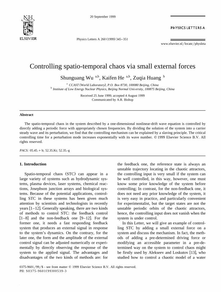
Ž . Ž .Fig. 1. Power spectrum of potential at fixed z zsp before aŽ .and after b control. The time interval, Dt, between consecutive

samples is 0.5, 1024 points are used to do the FFT, the totalnumber of sample points are 4096.

characteristic frequency region of the chaotic attrac-Ž .tor. For example, Fig. 1 a shows the spectrum of the

STC state to be controlled, from this figure one canŽsee that except for the frequency of driving wave V

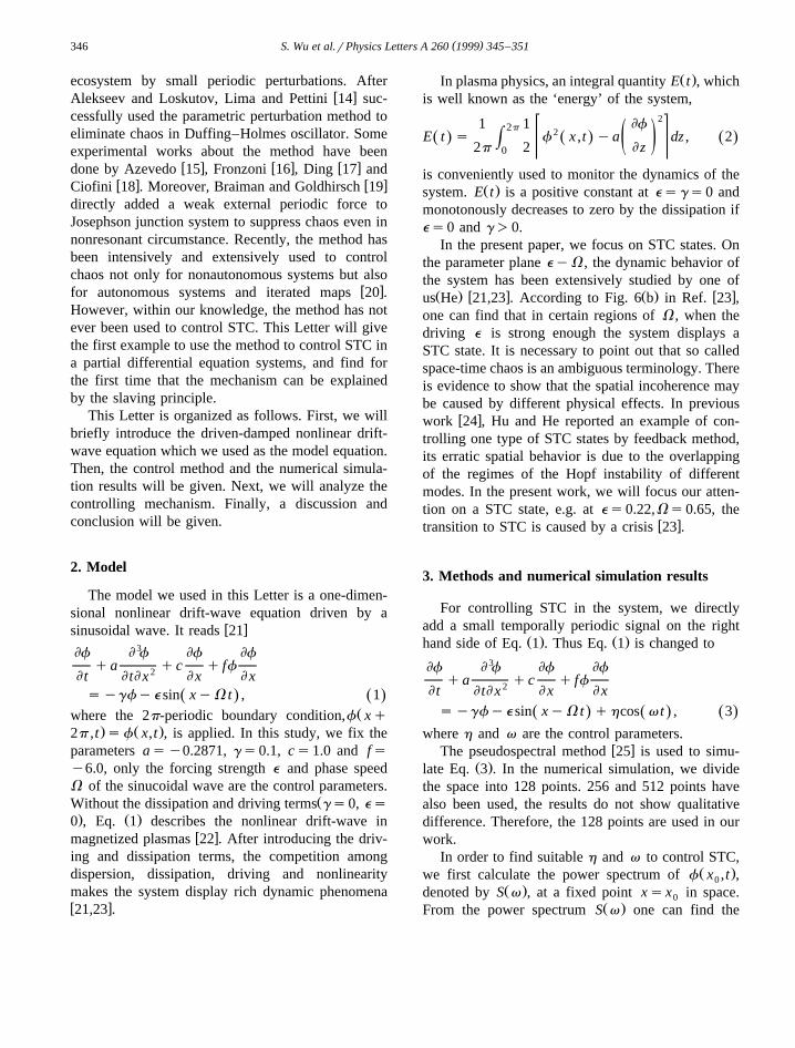
.s0.65 , there are many peaks in the region vgw x0.2,0.9 . Our experience shows that the appropriatev for a successful control should be chosen in thisregion. Now, fix an v in this region, one can try tofind a suitable h. We find some windows in v–h

plane, with which parameters the turbulent motion ofthe STC state can be successfully suppressed. Theresults are given in Fig. 2, in which the circles standfor the suitable parameter points for controlling STC

Ž .in system 1 , while the crosses indicate the parame-

Fig. 2. Global view of control parameters on the plane v –h.Points ` and = stand for the suitable and unsuitable parameter

Ž .points for controlling STC in system 1 , respectively.

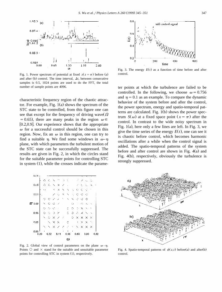
Ž .Fig. 3. The energy E t as a function of time before and aftercontrol.

ter points at which the turbulence are failed to becontrolled. In the following, we choose vs0.756and hs0.1 as an example. To compare the dynamicbehavior of the system before and after the control,the power spectrum, energy and spatio-temporal pat-

Ž .terns are calculated. Fig. 1 b shows the power spec-Ž . Ž .trum S v at a fixed space point xsp after the

control. In contrast to the wide noisy spectrum inŽ .Fig. 1 a , here only a few lines are left. In Fig. 3, we

Ž .give the time series of the energy E t , one can see itis chaotic before control, which becomes harmonicoscillations after a while when the control signal isadded. The spatio-temporal patterns of the system

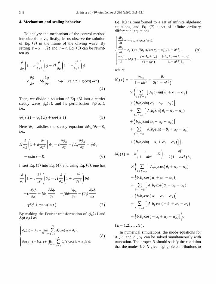
Ž .before and after control are shown in Fig. 4 a andŽ .Fig. 4 b , respectively, obviously the turbulence is

strongly suppressed.

Ž . Ž . Ž .Fig. 4. Spatio-temporal patterns of f z,t before a and after bcontrol.

( )S. Wu et al.rPhysics Letters A 260 1999 345–351348

4. Mechanism and scaling behavior

To analyze the mechanism of the control methodintroduced above, firstly, let us observe the solution

Ž .of Eq. 3 in the frame of the driving wave. ByŽ .setting zsxyV t and ts t, Eq. 3 can be rewrit-

ten as

E E 2 E E 2

1qa fsV 1qa f2 2ž / ž /Et E zE z E z

Ef Efyc y ff ygfye sin zqhcos vt .Ž .

E z E z4Ž .

Ž .Then, we divide a solution of Eq. 3 into a carrierŽ . Ž .steady wave f z , and its perturbation df z,t ,0

i.e.,

f z ,t sf z qdf z ,t . 5Ž . Ž . Ž . Ž .0

Here f satisfies the steady equation Ef rEts0,0 0

i.e.,

E E 2 Ef Ef0 0V 1qa f yc y ff ygf0 0 02ž /E z E z E zE z

ye sin zs0. 6Ž .

Ž . Ž . Ž .Insert Eq. 5 into Eq. 4 , and using Eq. 6 , one has

E E 2 E E 2

1qa dfsV 1qa df2 2ž / ž /Et E zE z E z

Edf Edf Ef Edf0yc y ff yfdf y fdf0E z E z E z E z

ygdfqhcos vt . 7Ž . Ž .

Ž .By making the Fourier transformation of f z and0Ž .df z,t as

N°Ž . Ž .f z s A q lim A cos kzqu ,Ý0 0 k k

N™` k s1~ 8Ž .N

Ž . Ž . Ž . Ž .df z ,t s b t q lim b t cos kzq a t ,Ž .Ý0 k k¢ N™` k s1

Ž .Eq. 6 is transformed to a set of infinite algebraicŽ .equations, and Eq. 7 a set of infinite ordinary

differential equations

db0° Ž .syg b qhcos v t ,0dtdbk 2~ Ž . Ž .Ž .s N t q f kb A sin u y a r 1y ak , 9Ž .k 0 k k kdt

Ž . Ž .da f k A q b f kb A cos u y ak 0 0 0 k k kŽ .s M t y y ,k¢ 2 2dt Ž . Ž .1y ak 1y ak bk

where

g b fkkN t sy qŽ .k 2 21yak 2 1yakŽ .

= X XA b sin u qa yaŽ .Ý l l l l k½Xlql sk

1X Xq b b sin a qa yaŽ .l l l l k2

X Xq A b sin u ya yaŽ .Ý l l l l kXlyl sk

1X Xq b b sin a ya yaŽ .l l l l k2

X Xq A b sin yu qa yaŽ .Ý l l l l kXl ylsk

1X Xq b b sin ya qa ya ,Ž .l l l l k2 5

c kfM t syk yV yŽ .k 2 2ž /1yak 2 1yak bŽ . k

= X XA b cos u qa yaŽ .Ý l l l l k½Xlql sk

1X Xq b b cos a qa yaŽ .l l l l k2

X Xq A b cos u ya yaŽ .Ý l l l l kXlyl sk

1X Xq b b cos a ya yaŽ .l l l l k2

X Xq A b cos yu qa yaŽ .Ý l l l l kXl ylsk

1X Xq b b cos ya qa ya ,Ž .l l l l k2 5

ks1,2, . . . , N .Ž .In numerical simulations, the mode equations for

A ,u and b ,a can be solved simultaneously withk k k k

truncation. The proper N should satisfy the conditionthat the modes k)N give negligible contributions to

( )S. Wu et al.rPhysics Letters A 260 1999 345–351 349

w xthe actual solution of the equation 24 . For thepresent parameters we use Ns13, i.e., the 27-di-mensional ordinary differential equations will besolved. With these mode equations one can obtainqualitatively the same results as the direct simulating

Ž .Eq. 3 .Now let us analyze the numerical results of the

Ž .solution of Eq. 9 . From the time evolution curvesof b , one can see that, for every mode k, therek

exists a turning point t ) , before which b showsk k

chaotic motion with larger amplitude, while after

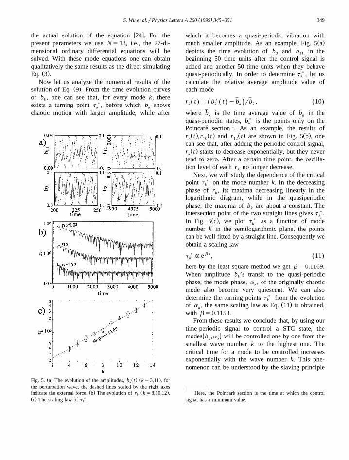
Ž . Ž . Ž .Fig. 5. a The evolution of the amplitudes, b t ks3,11 , fork

the perturbation wave, the dashed lines scaled by the right axesŽ . Ž .indicate the external force. b The evolution of r ks8,10,12 .k

Ž . )c The scaling law of t .k

which it becomes a quasi-periodic vibration withŽ .much smaller amplitude. As an example, Fig. 5 a

depicts the time evolution of b and b in the3 11

beginning 50 time units after the control signal isadded and another 50 time units when they behavequasi-periodically. In order to determine t ) , let usk

calculate the relative average amplitude value ofeach mode

)r t s b t yb rb , 10Ž . Ž . Ž .Ž .k k k k

where b is the time average value of b in thek k

quasi-periodic states, b) is the points only on thek

Poincare section 1. As an example, the results of´Ž . Ž . Ž . Ž .r t ,r t and r t are shown in Fig. 5 b , one8 10 12

can see that, after adding the periodic control signal,Ž .r t starts to decrease exponentially, but they neverk

tend to zero. After a certain time point, the oscilla-tion level of each r no longer decrease.k

Next, we will study the dependence of the criticalpoint t ) on the mode number k. In the decreasingk

phase of r , its maxima decreasing linearly in thek

logarithmic diagram, while in the quasiperiodicphase, the maxima of b are about a constant. Thek

intersection point of the two straight lines gives t ).kŽ . )In Fig. 5 c , we plot t as a function of modek

number k in the semilogarithmic plane, the pointscan be well fitted by a straight line. Consequently weobtain a scaling law

t ) Ae b k , 11Ž .k

here by the least square method we get bs0.1169.When amplitude b ’s transit to the quasi-periodick

phase, the mode phase, a , of the originally chaotick

mode also become very quiescent. We can alsodetermine the turning points t ) from the evolutionk

Ž .of a , the same scaling law as Eq. 11 is obtained,k

with bs0.1158.From these results we conclude that, by using our

time-periodic signal to control a STC state, the� 4modes b ,a will be controlled one by one from thek k

smallest wave number k to the highest one. Thecritical time for a mode to be controlled increasesexponentially with the wave number k. This phe-nomenon can be understood by the slaving principle

1 Here, the Poincare section is the time at which the control´signal has a minimum value.

( )S. Wu et al.rPhysics Letters A 260 1999 345–351350

w xin synergetics 26 . From the first equation of Eq.Ž .9 , one can see that, in fact, the external force isadded on the mode ks0, the evolution of b is0

uniquely determined by the applied control signaland the dissipation rate g . Its motion does not influ-enced by the other k/0 modes. The motion of b is0

adjusted to periodic one very quickly after the con-trol signal is added. Then the other modes k/0 are

Ž .slaved by b . This fact can be seen from Eq. 9 for0

k/0. In both equations for b and a , there is ak k

term depending on b , which is the contribution of0� 4the mode-mode couplings between b , A ,u and0 k k

� 4b ,a . Through these terms b plays the slavingk k 0

role. Meanwhile, since the modes of the steady waveŽ . � 4 � 4f z , A ,u are constants in the frame of z,t .0 k k

� 4the modes b ,a also play a significant role in thek k

solving process. Moreover, the numerical results tellus that b is a slowly relaxing variable and the other0

modes are fast ones in the beginning stage when thecontrol signal is just added. Thus, b plays an0

important role as an order parameter in the system,and it is affected by the control force. When thecontrol signal is added, b and a are immediately1 1

� 4slaved by b . Since the effect of b on b ,a is0 0 k k� 4through A ,u and A decrease with k™`, thek k k

slaving intensity is not unform for different modes.Ž .From Eq. 9 , one can see that the smaller the mode

k, the higher the slaving intensity it has. So the modeks1 can be controlled firstly. Then, it starts to slavethe modes ks2,3, . . . , until all the modes are tamed.In the whole process, the system changes from an

Ž .extremely disordered a STC state into an orderedone by the self-organization principle.

5. Conclusion and discussion

In conclusion, we have successfully suppressedvery turbulent STC states by directly adding a tem-porally periodic force on the system. The appropriateinput frequency can be chosen by analyzing thespectrum of the turbulence. In contrast to the feed-back method for which one needs the knowledge ofthe target state, the present method is easy to berealized in practical experiments. The controllingmechanism is studied by investigating the evolutionof perturbation wave to the carrier steady wave. Wefind that the perturbation modes are controlled one-

by-one from long to short wave length by a slavingprinciple, and the critical controlling time for themode increases exponentially with its wave numberk. Since the slaving effect is very important innonlinear science, these results may be interested inby scientists and engineers. The schemes of how toselect the controlling frequency may also be helpfulfor the experimentalists.

Acknowledgements

Ž .The first author S.W. would like to thank Drs.Baisong Xie and Luqun Zhou for useful discussions.This work is supported by the National NaturalScience Foundation of China under grant No.19675006, No. 19835020 and the Research Fundsfor the Doctoral Program of Higher Education underthe grant No. 98002713.

References

w x Ž .1 G. Hu, Z. Qu, Phys. Rev. Lett. 72 1994 68.w x Ž .2 D. Auerbach, Phys. Rev. Lett. 72 1994 1184.w x Ž .3 F. Qin, E.E. Wolf, H.-C. Chang, Phys. Rev. Lett. 72 1994

1459.w x Ž .4 G. Hu, Z. Qu, K. He, Int. J. Bifurc. Chaos 5 1995 901.w x Ž .5 W. Lu, D. Yu, R.G. Harrison, Phys. Rev. Lett. 76 1996

3316.w x6 E. Tziperman, H. Scher, S.E. Zebiak, M.A. Cane, Phys. Rev.

Ž .Lett. 79 1997 1034.w x7 R.O. Grigoriev, M.C. Cross, H.G. Schuster, Phys. Rev. Lett.

Ž .79 1997 2795.w x Ž .8 P. Parmananda, Yu. Jiang, Phys. Lett. A 231 1997 159.w x9 I. Aranson, H. Levine, L. Tsimring, Phys. Rev. Lett. 72

Ž .1994 2561.w x Ž .10 Y. Braiman, J.F. Lindner, W.L. Ditto, Nature London 378

Ž .1995 465.w x11 N. Parekh, S. Parthasarathy, S. Sinha, Phys. Rev. Lett. 81

Ž .1998 1401.w x Ž .12 R. Montagne, P. Colet, Int. J. Bifurc. Chaos 8 1998 1849.w x Ž .13 V.V. Alekseev, A.Y. Loskutov, Soviet Phys. Dokl. 32 1987

1346.w x Ž .14 R. Lima, M. Pettini, Phys. Rev. A 41 1989 726.w x Ž .15 A. Azevedo, S.M. Rezende, Phys. Rev. Lett. 66 1991 1342.w x16 L. Fronzoni, M. Giocondo, M. Pettini, Phys. Rev. A 43

Ž .1991 6483.w x17 W.X. Ding, H.Q. She, W. Huang, C.X. Yu, Phys. Rev. Lett.

Ž .72 1994 96.w x Ž .18 M. Ciofini, R. Meucci, F.T. Arecchi, Phys. Rev. E 52 1995

94.w x Ž .19 Y. Braiman, I. Goldhirsch, Phys. Rev. Lett. 66 1991 2545.

( )S. Wu et al.rPhysics Letters A 260 1999 345–351 351

w x20 D. Cai, A.R. Bishop, N. Gronbech-Jensen, B.A. Malomed,Ž .Phys. Rev. E 49 1994 1000; G. Cicogna, L. Fronzoni, Phys.

Ž .Rev. E 47 1993 4585; D. Iracane, P. Bamas, Phys. Rev.Ž .Lett. 67 1991 3086; Y.S. Kivshar, F. Rodelsperger, H.

Ž .Benner, Phys. Rev. E 49 1994 319; Z.L. Qu, G. Hu, G.J.Ž .Yang, G.R. Qin, Phys. Rev. Lett. 74 1994 1736; E.F.

Ž .Stone, Phys. Lett. A 163 1992 367; S.T. Vohra, L. Fabiny,Ž .K. Wiesenfeld, Phys. Rev. Lett. 72 1994 1333; Y. Liu,

Ž .J.R.R. Leite, Phys. Lett. A 185 1994 35; R.-R. Hsu, H.-T.Ž .Su, J.-L. Chern, C.-C. Chen, Phys. Rev. Lett. 78 1997

2936.

w x21 K. He, A. Salat, Plasma Phys. and Controlled Fusion 31Ž .1989 123.

w x22 V. Oraevskii, H. Tasso, H. Wobig, in: Proc. 3rd Int. Conf.Plasma Physics and Controlled Nuclear Fusion Research,

Ž .Novosibirsk, 1968 IAEA, Vienna, 1969 vol. 1, p. 167.w x Ž .23 K. He, Phys. Rev. Lett. 80 1998 696.w x Ž .24 G. Hu, K. He, Phys. Rev. Lett. 71 1993 3794.w x Ž . Ž .25 S.A. Orszag, Studies in Applied Mathematics L 4 1971

293.w x26 H. Haken, Synergetics, An Introduction, 2nd Ed. Springer-

Verlag, BerlinrHeidelbergrNew York, 1978.