770

Spatio-Temporal Complexity in Nonlinear Image Processing

JAMES P. CRUTCHFIELD

Ahsfruct -This is a pictorial survey of pattern dynamics in video feed- back and in related numerical models. After a short introduction to video feedback apparatus and concepts from dynamical systems theory, a range of phenomena are presented, from simple attractor types to homogeneous video turbulence. Examples of complex behavior include symmet~y-locking chaos, spatial amplification of fluctuations in open flows, dislocations, phyllotaxis, spiral waves, and noise-driven oscillations. Video experiment5 on nonlinear transformations of the plane are also described. The suney closes with a discussion of the relationship between dgnamical systems and nonlinear, iterative image processing.

Keywords - Attractor, basin, chaos, coherence, complexity, dimension, dislocations, entropy, flows, image processing. lattice dynamical system\, limit cycle, mappings, partial differential equations, phyllotaxi5. reaction- diffusion, spatially extended systems, spiral waves, transients, turbulence, video feedback.

I . INTRODUCTION HAOS is now the most notorious [l] and well-studied C [2], [ 3 ] source of complex behavior arising in nonlin-

ear deterministic processes. The specific complexity-gener- ating mechanisms referred to under this rubric are not the entire story, however. As the following pictorial survey will demonstrate, complexity in spatio-temporal systems de- mands substantial generalizations to the basic theory of dynamical systems and to our present appreciation of the diverse forms manifested by the interplay of randomness and order. Although chaos is only one of many complex phenomena, the rapid progress made in its understanding gives hope that the diversity of spatio-temporal behavior will also yield to a similar “experimental mathematical” approach [4].

Indeed, the particular spatial systems presented in the following, video feedback [SI and lattice dynamical systems [6], were taken up in order to address the larger questions of just how dynamical systems theory, as developed for understanding low-dimensional chaos, could be applied to a wider range of physical processes, viz. those whose behavior depends on time and on space. Along the way a number of new phenomena and connections with well- known behavior were discovered. This pictorial survey is concerned with this phenomenology as it appears in two

Manuscript received September 10. 1987. This work wab supported in part by the Office of Naval Research under Grant N00014-86-K-0154. The numencal simulations were performed on a Cray X/MP and o n ;L

Sun Microsvstem workstation with a Mercun Computer Systems ZIP 3232 array processor. The former was fundcd by the Cray-Sponsored University Research and Development Grant Program

The author is with the Physics Department. University of California. Berkeley, CA 94720.

IEEE Log Number 8821323.

spatial dimensions. First, though, basic notions from dy- namical systems and the apparatus of video feedback must be introduced. After presenting a range of different phe- nomena in video feedback and related numerical models, the discussion closes by addressing several general ques- tions of interest to enginecring. Specifically, the last section considers the relevance of the experimental-mathematical approach to the “engineering” of nonlinear image pro- cessing systems.

11. VIIEO FEEDBACK Space does not allow a detailed introduction to the

topics covered in the following sections (the reader is referred to a paper [SI and references therein. and to a videotape [7] for this). I n the former, a more complete discussion of the experiment5 and related video physics is presented. In the latter. excerpts from various experiments can be seen evolving in time. Since one of the major focal points is the complexity of time-dependent behavior, the videotape is a substantid improvement over the static images required by a conventional publication format. An even better approach is for the reader to experiment with video feedback directly. which is highly encouraged. Al- though scientific experimi:nt.ition requires careful calibra- tion and instrumentation quality equipment. most of the phenomena described below can be observed in consumer grade video equipment M ith patient investigation. For an introduction to luttice d lwm;cu l systrnis, a class of numeri- cal models that evolved out of the video feedback investi- gations. see [6].

The basic configuratioil of a video feedback system is quite simple. When a vidvo camera is directed at a display monitor, to which it is connected, a feedback loop is closed. Two-dimensional images I( x. JI) from the monitor screen impinge on the camera’s photodetector after passing through space and optical processing elements. The camera dissects the image into ai1 electronic signal V ( t ) by ruster scanning the intensity profile on the photodetector into a temporal sequence of horizontal lines. The video signal V ( t ) gives the intensity of a point, or pixel, along a raster scan line at time t . The signal arrives at the monitor after electronic processing and is reconstructed as a two-dimen- sional image on its screcn. Thus as i t flows around the loop, there are two dom;iins in which the image informa- tion can be processed: optic;il and electronic.

Optical image processing often consists passing the image through various lens s, stems that control the light inten-

0098-4094/S8/0700-0770$01 .OO ‘ 1988 IEEE

CRIJTCHFILLD: COMPLEXITY IN NONLINEAR IMAGE PROCESSING 771

sity gain (iris), image focus, and spatial magnification and filtering. There might also be nonlocal image processing, such as image translation or rotation. The latter can be effected by mounting the camera so that it rotates about its optical axis. Electronic processing provides spatially local image processing as it operates directly on the in- stantaneous intensity signal V( t ) , that is, on horizontal and possibly vertical pixel neighborhoods. Electronic image processors provide modules to handle the basic video frame and line~synchronization, to add and multiply images point by point, and to perform nonlinear pixel and pixel neighborhood transformations [8]. Spatially nonlocal elec- tronic image processing can be performed by manipulating the raster geometry itself and displaying the result on a suitably modified monitor [9].

A question that frequently arises in using electronic systems to investigate theoretical problems of complexity is whether the process involved is a simulation or an experiment. The distinction is somewhat moot as long as science is served. Nonetheless, it should be said that once the functional elements are well characterized, video feed- back as an experiment becomes video feedback as simula- tion. This is simply a change in the experimenter’s attitude rather than in the apparatus or the phenomena observed. Speaking broadly, as a simulator video feedback allows one to study the class of systems, called reaction-diffusion partial differential equations introduced by Alan Turing [lo]. It can do much more than this, though, such as simulate spin glasses, neutral networks, delay-partial-dif- ferential equations, multi-species chemical reactions, and so on. Discussion of these systems is beyond this survey’s scope.

111. DYNAMICAL SYSTEMS A central motivation in studying video feedback has

been to understand how the geometric picture and statisti- cal methods of dynamical systems theory can be gen- eralized to explain the complexity observed in time- dependent pattern generating systems. Thus to put the investigation in the proper framework, the following sec- tion introduces a few notions from dynamical systems theory [2], [3] that will be used later on.

The primary abstraction of dynamical systems theory is that the instantaneous configuration of a process is repre- sented as a point, or state, in a space of states. The dimension of the space is the number of numbers required to uniquely specify the configuration of the process at each instant. With this, the temporal evolution of the process becomes the motion from state to state along an orbit or trajectory in the state space.

For video feedback the space of states is the space of two-spatial-dimension patterns I ( x, y ). For a mono- chrome system I ( x , y ) is the intensity at a point (x, y ) on the screen; for color, I consists of a vector of red, green, and blue intensity components. The dimension of the equivalent dynamical system is given by the effective num- ber of pixels. For the behavior described below a (rough) upper bound of the dimension of the state space is

250 000 ( = 5122). The temporal evolution of patterns is thus abstractly associated with a trajectory in this high-di- mensional state space. If the behavior is simple, however, then the trajectory can be pictured as moving in a much lower dimensional subspace.

If a temporal sequence of patterns is observed to be stable under perturbations, then we assume that the trajectory lies on some attractor in pattern space. One of the main contributions of dynamical systems theory’ is the categorization of all long-term behavior into three attrac- tor classes: fixed point, limit cycle, and chaotic attractors. A fixed point attractor is a single, isolated state toward whch all neighboring states evolve. A limit cycle is a sequence of states that are repetitively visited. One can also have a “product” of limit cycle oscillators, called a torus and denoted T“ where n is the number of con- stituent cycles. These attractors describe predictable be- havior: two nearby states on such an attractor stay close as they evolve. Unpredictable behavior, for which the latter property is not true, is described by chaotic attractors. These are often defined negatively as attractors that are neither fixed points, limit c!cles, nor tori.

Aside from attractor classification, another significant contribution of dynamical systems theory is a geometric picture of how transients relax onto the attractors. An attractor’s basin of attraction is the set of all points that evolve onto the attractor. There can be multiple basins and attractors, so that radically different behavior may be seen depending on the initial Configuration. The complete cata- log of attractors and their basins for a given dynamical system is called its attractor-basin portrait.

Finally, dynamical systems theory is also the study of how attractors and basin structures change with the varia- tion of external control parameters. A bifurcation occurs if , with the smooth variation of a control, the attractor-basin portrait changes qualitatively.

To summarize, dynamical systems theory is a language that describes how complexity arises in (i) asymptotic behavior, (ii) basin structure, and (iii) bifurcations. I t forms a natural framework with which to explore the complex spatio-temporal dlnamics of video feedback. The pictorial essay which follows is organized along the par- ticular phenomena that ha\e been observed in video feed- back. The sections are mort: or less independent.

IV. BASIC SPATIO-TEMPORAL ATTRACTOR TYPES This section demonstrates the basic attractor types: fixed

points as time-independent equilibrium patterns, limit cycles as periodic image sequences, and a chaotic attractor arising from the competition of marginally stable symme- tries.

Photo 1 shows a time-independent and stable pattern. The dynamical system description of this is a fixed point in the space of patterns. Although there are very simple fixed point patterns, such AS an entirely dark image, the one shown is complex. This emphasizes an important

Only dissipative dynamical systi’ms will be described here.

772 ILEE TRANSACTIONS ON CIKCUITS A N I ) S Y S I t M S , ”01~. 35, NO 7. 1IJI.Y 19x8

distinction with conventional theory in whch one does not associate any intrinsic complexity with a fixed point. In the case of spatially-extended systems, measuring the com- plexity even of fixed points is clearly desirable. Quantifica- tion of spatial complexity, however, is fraught with diffi- culties at present.

Photos 2, 3 and 4 give three snapshots during one cycle of a periodic sequence of patterns. This is a limit cycle in pattern space and is stable under small perturbations.

Photos 5 through 8 show a sequence of snapshots from an aperiodic image sequence. Here there are two marginal- ly stable patterns of fourfold and 21-fold symmetries. The trajectory visits neighborhoods of these patterns intermit- tently. Analysis of the time-dependent Fourier amplitudes of the underlying symmetric pattern shows the behavior is described by low-dimensional dynamics and is globally stable, and that starting from nearby patterns orbits sep- arate rapidly. Thus, the behavior is most likely described by a chaotic attractor, although the (necessary) measure- ment of the metric entropy has yet to be carried out.

V. DISLOCATION DYNAMICS Photos 9 and 10 show the interdigitated light and dark

fingers of video dislocations. Similar patterns occur in a wide range of physical and biological systems, such as:

convection cell patterns found in Rayleigh-BCnard and Couette fluid flows and in liquid crystal flows; domains in two-dimensional (anisotropic) spin sys- tems, such as thin magnets used for magnetic bubble devices; labyrinthine patterns in ferrofluids; flux patterns in type I1 superconductors; and the ocular dominance pattern in the visual cortex.

While the particular mechanisms responsible for disloca- tions in these examples differ greatly, there is a common element. In each there is an “order parameter” that alter- nates between saturation extremes over some fixed spatial length scale. The order parameter in each of the examples above is (1) the direction of fluid flow, charge transport, or (2) local magnetization; (3) the existence or absence of ferrofluid; (4) the local conductivity, and ( 5 ) the variation of left or right visual field associated with cortex columns.

The diversity of examples calls for a general definition of dislocations. They can be defined as the localized de- fects arising from the breaking of a pattern’s underlying spatial symmetry. The patterns that exhibit the exact sym- metry are the “ground” or “ vacuum” states. The lowest energy perturbations from these equilibrium states are dislocations.

A wide range of dislocation dynamics is readily ob- served. In the typical evolution from a random initial pattern, the system first establishes the characteristic spa- tial wavelength and produces a tangle of “frustrated” fingers with many dislocations. The dislocations collide and annihilate and the pattern becomes more regular. At this point the system may continue to evolve toward less

complex patterns or it may begin to spontaneously create dislocations. In the former case, the attractor is a fixed point reached by a complex transient. In the latter case, the attractor manifests itself as a pattern sequence of a ‘‘gas’’ of capriciously-moving dislocations, whose creation and annihilation rates balance. One of the interesting questions here is how to describe the underlying state space structures [ll].

Dislocations result from the interplay of two processes. The first is the local bistability of the order parameter. Values of the order parameter intermediate between the saturation extremes are unstable. The second is “lateral inhibition”, to borrow a phrase from neurophysiology. This imposes the spatial length scale over which the order parameter alternates by forcing neighbors bordering a region into the opposite xaturation state from the region itself.

In video feedback, dislocations are found when using photoconductor-based cameras at high beam current. I t appears that secondary electrons are scattered from the beam spot to neighboring regions. In a relative sense, this reduces photosensitivity in those regions when the beam scans illuminated photoconductor and increases it when the beam scans dark photoconductor.

A simple numerical model of dislocations that embodies these processes is given by the following discrete time and space lattice dynamical .spteni [6]:

f ( x > = x - k sin(2nx)

is the state a site ?at time n ; indexes the site in a d-dimensional lattice; is a relatiyeendex to the neighbor- ing sites N ( i ) ; are the coupling kernel coefficients which control the lateral inhibition- and set the finger width. For site i and possibly its near neighbors, the coefficients are positive. This gives a diffusive coupling. For sites fur- ther away, the coefficients are negative which gives inhibitory coupling;

for k > 0 gives the stable satura- tion values of x = 0 and x = 1. This function is related to the widely studied map of the circle [2].

Photos 11, 12, and 13 show the relaxation from a random initial pattern in a d = 2 lattice after 20, 100, and 1100 iterations. Here a 90” rotation of the image is per- formed on eackiteration by a suitably chosen nonlocal neighborhood N . The system ultimately relaxes, through

CRUTCHFIELD: COMPLEXITY IN NONLINEAR I .WGt PROCESSING 173

the collision and annihilation of dislocations, onto a fixed point attractor consisting of concentric rings.

VI. COUPLED RELAXATION OSCILLATORS Many physical, chemical, biological, and engineering

systems can be described as coupled relaxation oscillators. Each oscillator plays the role of a local clock: counting up and resetting to some reference state. While the coupling communicates the local phase information to accelerate or retard neighboring oscillators. This section illustrates some of the spatio-temporal patterns that can emerge from this combination: spiral waves and transient spatial chaos.

Spiral waves occur in an active medium with periodic local dynamics diffusively coupled. The most famous ex- ample of this behavior is the Belousov-Zhabotinsky chem- ical reaction [12]. Photos 14, 15, and 16 show the center of three different spiral waves with one, two, and three spiral arms [13] found in video feedback experiments. Dynami- cally every point in the pattern has a well-defined oscilla- tion phase except for the spiral center where there is a phase singularity. In each photo the distinct colors label stages of the local oscillations.

The second example is a model of a water layer dripping from a flat surface. The equations of motion are similar to that for the dislocation model, except there is simple spatial averaging (all c, = constant) and the local piece- wise-linear dynamics is f( x) = w + sx (mod 1). The param- eter o gives the increment in the local variable on each iteration. T h s determines, if s =1, the clock’s period. The parameter s controls the slope which determines the clock’s stability: if s < 1 the cycles will be stable. The (modl) operation performs the resetting or dripping of a thick region of the water layer.

Photos 17 and 18 show the patterns after 310 and 492 steps starting from a uniform pattern with the center site slightly perturbed. and from a random initial pattern, respectively. Although these patterns appear complex, eventually both decay to simple periodic behavior. Thus the observed complexity is only a transient. The surprising result is that for this very simple system the length of the transients grows hyper-exponentially with increasing sys- tem size [ I l l . This is somewhat disturbing since one would have to wait, for the examples shown here, many universe lifetimes to observe the system’s attractor. This is a clear example of spatio-temporal complexity that is not de- scribed by a chaotic attractor.

VII. LOGARITHMIC SPIRALS A N D PHYLLOTAXIS A common large-scale symmetry found in video feed-

back patterns is the logarithmic spiral illustrated by Photo 19. This is a natural consequence of camera rotation and optical demagnification. On each circuit of the feedback loop the image is rotated and reduced in size, leading to a sea-shell-like self-similarity.

Biological patterns appear in other regimes as well. Photos 20 and 21 show “crystalline” lattices of stable, isolated dots. In the first the dots at the center fall into a phyllotaxic symmetry. Phyllotaxis refers to the arrange-

ment of leaves on a stem or florets in a composite flower, such as a sunflower, along logarithmic spirals. The second photo (21) illustrates a more complex lattice with domains of simple symmetries separated by walls.

VIII. OPEN FLOWS A N D THE SPATIAL AMPLIFICATIOPI OF FLUCTUATIONS

There is a wide class of physical phenomena in which material transport through a system leads to the spatial magnification of small fluctuations. This in turn results in complex macroscopic structure downstream. Open flows, such as pipe flow, are the most well-known examples of this [14]. The structures forrned downstream, such as vortex streets or turbulent plugs, are supported in a sense only by the fluctuations: the ideal noiseless systems admit regular flows.

This class of systems is (easily studied with video feed- back by simply offsetting the camera and monitor centers. With the camera unrotated and offset upwards, for exam- ple, successive images are seen displaced downwards on the monitor. When nonlinear electronic processing is add- ed and the local dynamics becomes unstable small fluctua- tions at the screen top are magnified and propagate down the screen. Photos 22, 23, and 24 show a “waterfall” where perturbations propagate down the screen. The first photo 22 shows the initial development from a small fluctuation on the photo’s right side. The second (23) and third (24) photos show its growth and propagation’ downscreen.

Photos 25 and 26 illustrate another example of how small fluctuations are filtered into manifesting themselves as structured macroscopic patterns. In this situation noise drives relaxation-type oscillations. Here large spatial mag- nification and light gain make the video system sensitive to small fluctuations. If of sufficient size, the fluctuations are amplified and filtered spatially and temporally to macro- scopic observable patterns. Typically, only a few “amplifi- cation” pathways are seen; two of which are shown in the photos.

Ix. BIFURCATIONS

The foregoing survey has concentrated on the wealth of pattern dynamics arising at particular control settings. Video feedback, much like any analog computer, does not reveal its unique benefits as a real-time investigative tool until one realizes all this phenomenology can be interac- tively changed and the results immediately seen. This leads to the study of bifurcations through which qualitative changes in the dynamics occur with the smooth variation of control parameters.

9.1. Symmetry Locking and Chuos The majority of patterns seen so far have exhibited

azimuthal symmetry which has been imposed on the image by camera rotation. The ninefold symmetry seen in the video dislocation photos corresponds to a camera rotation of 40 degrees. The effect camera rotation has on behavior can be studied in isolation in the following way. First, the

I14

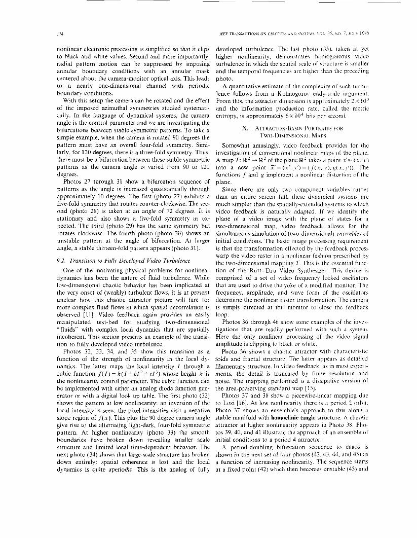
nonlinear electronic processing is simplified so that it clips to black and whte values. Second and more importantly, radial pattern motion can be suppressed by imposing annular boundary conditions with an annular mask centered about the camera-monitor optical axis. T h s leads to a nearly one-dimensional channel with periodic boundary conditions.

With t h s setup the camera can be rotated and the effect of the imposed azimuthal symmetries studied systemati- cally. In the language of dynamical systems, the camera angle is the control parameter and we are investigating the bifurcations between stable symmetric patterns. To take a simple example, when the camera is rotated 90 degrees the pattern must have an overall four-fold symmetry. Simi- larly, for 120 degrees, there is a three-fold symmetry. Thus, there must be a bifurcation between these stable symmetric patterns as the camera angle is varied from 90 to 120 degrees.

Photos 27 through 31 show a bifurcation sequence of patterns as the angle is increased quasistatically through approximately 10 degrees. The first (photo 27) exhibits a five-fold symmetry that rotates counter-clockwise. The sec- ond (photo 28) is taken at an angle of 72 degrees. It is stationary and also shows a five-fold symmetry as ex- pected. The third (photo 29) has the same symmetry but rotates clockwise. The fourth photo (photo 30) shows an unstable pattern at the angle of bifurcation. At larger angle, a stable thirteen-fold pattern appears (photo 31).

9.2. Transition to Fully Developed Video Turbulence One of the motivating physical problems for nonlinear

dynamics has been the nature of fluid turbulence. Whle low-dimensional chaotic behavior has been implicated at the very onset of (weakly) turbulent flows, it is at present unclear how this chaotic attractor picture will fare for more complex fluid flows in whch spatial decorrelation is observed [ l l ] . Video feedback again provides an easily manipulated test-bed for studying two-dimensional “ fluids” with complex local dynamics that are spatially incoherent. This section presents an example of the transi- tion to fully developed video turbulence.

Photos 32, 33, 34, and 35 show this transition as a function of the strength of nonlinearity in the local dy- namics. The latter maps the local intensity Z through a cubic function f ( Z ) = h ( Z + bZ2 + cZ3) whose height h is the nonlinearity control parameter. The cubic function can be implemented with either an analog diode function gen- erator or with a digital look up table. The first photo (32) shows the pattern at low nonlinearity: an inversion of the local intensity is seen; the pixel intensities visit a negative slope region of f ( x ) . T h s plus the 90 degree camera angle give rise to the alternating light-dark, four-fold symmetric pattern. At higher nonlinearity (photo 33) the smooth boundaries have broken down revealing smaller scale structure and limited local time-dependent behavior. The next photo (34) shows that large-scale structure has broken down entirely: spatial coherence is lost and the local dynamics is quite aperiodic. This is the analog of fully

developed turbulence. The last photo (35). taken at yet hgher nonlinearity, demonstrates homogeneous video turbulence in whch the spatial scale of structure is smaller and the temporal frequencies are higher than the preceding photo.

A quantitative estimate of the complexity of such turbu- lence follows from a Kolmogorov eddy-scale argument. From ths , the attractor dimension is approximately 2 x 10’ and the information production rate, called the metric entropy, is approximately 6 X l o4 bits per second.

X. ATTRACTOR-BASIN PORTRAITS FOR TWO-DIMENSIONAL MAPS

Somewhat amusingly, video feedback provides for the investigation of conventional nonlinear maps of the plane. A map T: R * + R * of the plane R ’ takes a point x’= ( x . J ) into a new point 2’ = (x’, y’) = ( f ( x, y ) , g( x, y )). The functions f and g implement a nonlinear distortion of the plane.

Since there are only two component variables rather than an entire screen full, these dynamical systems are much simpler than the spatially-extended systems to which video feedback is naturally adapted. If we identify the plane of a video image with the plane of states for a two-dimensional map, \ideo feedback allows for the simultaneous simulation of (two-dimensional) en.ret~~11le.s of initial conditions. The basic image processing requirement is that the transformation effected by the feedback process warp the video raster in a nonlinear fashion prescribed by the two-dimensional mapping T. This is the essential func- tion of the Rutt-Etra Video Synthesizer. This device is comprised of a set of video frequency locked oscillators that are used to drive the yoke of a modified monitor. The frequency, amplitude, and wave form of the oscillators determine the nonlinear raster transformation. The camera is simply directed at this monitor to close the feedback

Photos 36 through 46 show some examples of the invea- tigations that are readily performed with such a system. Here the only nonlinear processing of the video signal amplitude is clipping to black or white.

Photo 36 shows a chaotic attractor with characteristic folds and fractal structure. The latter appears as detailed filamentary structure. In \-ideo feedback, as i n most experi- ments, the detail is truncated by finite resolution and noise. The mapping performed is a dissipative version of the area-preserving standard map [15).

Photos 37 and 38 show a piecewise-linear mapping due to Lozi [16]. At low nonlinearity there is a period 2 orbit. Photo 37 shows an ensemble’s approach to this along a stable manifold with homoclinic tangle structure. A chaotic attractor at hgher nonlinearity appears in Photo 38. Pho- tos 39, 40, and 41 illustrate the approach of an ensemble of initial conditions to a period 4 attractor.

A period-doubling bifurcation sequence to chaos is shown in the next set of four photos (42, 43. 44, and 45) as a function of increasing nonlinearity. The sequence starts at a fixed point (42) which then becomes unstable (43) and

loop.

CKtITCHI I tLD: COMPLLXIIY IN NONLINEAR IMAGE PROCESSING 775

relaxes onto a period two limit cycle (44). Photo 45 shows a two “band” chaotic attractor later in the bifurcation sequence.

Finally, with constant illumination, rather than a brief initial burst of light, the basin of attraction can be investi- gated. Photo 46 demonstrates the basin for a simple period 2 limit cycle.

XI. NONLINEAR IMAGE PROCESSING This survey has given only a brief introduction to the

contemporary study of spatially extended nonlinear dy- namical systems. In t h s endeavor, video feedback is seen to be a flexible, high-speed simulator, on the one hand, and a source of diverse spatio-temporal experimental data, on the other. The survey has not described many other types of complex behavior, such as, how video feedback can be used to implement neural networks, spin glasses, and multiple-species chemical reactions. Space has also not allowed for a discussion of the theoretical relationshp between information and dynamical systems theories that are so important in the analysis of this complexity [17]. We will close with a discussion of the relationship of this work to future directions in nonlinear image processing.

Some similarities with image processing systems are clear from the mathematical formulation of the models and from the video apparatus. The systems we have studied here are nonlinear iterative image processing systems. The diversity of behavior seen in video feedback indicates that incorporating both nonlinearity and iteration will lead to many new image processing techniques and to a broader theoretical framework for image processing based on dy- namical systems theory. From the point of view of dy- namical systems, image processing tasks suggest questions of how to design the attractors and basin structures of spatially extended dynamical systems to perform specific computation and image processing tasks and how to do these efficiently.

From a slightly different perspective, video feedback as presented here is an experimental exploration of the poten- tials of optical computing. The camera-monitor system is employed essentially as an image operational amplifier. As far as the methodology and the phenomena are concerned any technology could be used for this function. To date there appear to be no reasonable alternative optical op amps. If such an instrumentation-quality device were to become available, especially one that was truly parallel in operation then, for the investigation of two- and higher dimensional spatial dynamics, feedback optical computing would vastly outstrip digital computers of any architecture in speed and ease-of-use. The potential impact on the simulation of very complex scientific problems is hard to overestimate. Even with current video technology substan- tial progress along these lines could be made. The manu- facturers of broadcast quality and high definition televi- sion (HDTV) video equipment are in unique positions to establish laboratories for video feedback investigations of nonlinear spatially extended dynamics.

It is somewhat sobering to realize that the diversity of phenomena presented here could have been as easily in- vestigated thirty years ago as now. The basic technology for video feedback has been available since the 1950’s. If history is any indication. then, the alternative approach advocated here may be a route not taken. Despite their potential for scientific simulation, video feedback and re- lated image processing techniques could very well continue to be eclipsed by expensive multiple-processor su- percomputers. The resurgence in interest in optical computing, in distributed processing, and in parallel com- putational archtectures, however, are hopeful signs that interactive, high-speed machines for the experimental mathematical investigation of complexity may be widely available in the next decade. The next few years will tell if image processing and video feedback contribute directly to t h s line of technological development.

ACKNOWLEDGMENT This work has benefited greatly from the expertise of

Donald Day of the California College of Arts and Crafts. The two-dimensional mapping work was done in CCAC’s Video Department.

REF1 RENCES J. Gleick. Cliuos, Mukrrig i h ’ e ~ Scicric.c. Ne- York: Viking. 1987. P. Berge, Y . Pomeau, and C Vidal. Order II itliiri Cliuo,: Toitwd\ U Deterministic Approuch to Turhulenw. J. P. Crutchfield, N. H. Packard, J . D Farmer. and R. S Shaw, “Chaos,” Sci. A m . 255, vol. 46. Dec. 1986. D. Campbell, J. P. Crutchfie d. J . D. Farmer. and E. Jcn, “Expcri- mental mathematics: The rolt of computation in nonlinear studies.” Comm. A C M , vol. 28, p. 374. 1985. J. P. Crutchfield, “Space-tirnc dynamics in video fccdback.” PliL.situ vol. 10D, p. 229, 1984. J. P. Crutchfield and K. Kaneko, “ Phenorncnology of spatio-tem- poral chaos” in Direction.! in Chu0.s. (Hao Bai-Lin, Ed.) Singa- pore: World Scientific Publishers. 1087. J. P. Crutchfield, Spuce- T/rw D~ynuniic.\ it1 Video Ffwlbuc h und Chuotic Attructors of Driivn Osullurors. vidco tape, Aerial Prcsa. P.O. Box 1360, Santa Cruz. (TA 95064. 19x4. Pixel processing was perfoimed hv an analog irnagc processor designed by Dan Sandin o’ the Univcrsitb of Illinois. Chicago Circle, and by a max video digital image processor manufactured by Datacube, Inc. (Peabody, MA). For this we have used a Rutl-Etra Video Synthesizer While these are no longer manufactured, motlern digital video effects machines d o incorporate similar rast1.r nianrpulation functions. Quantel’h Miruge, Ampex’s ADO. and the more rccent Sony Reul-Time Texture-Mupping System x e examples. For the latter sec M. Oka. K. Tsutsui, A. Ohba, Y . Kur.iuchi, and T. Tago, “Real-time mani- pulation of texture-mapped surfaces,” Conip. Grcrphic..s, vol. 21. 181. 1987. A. M. Turing, “The chemical basis of morphogcncsis,” Trun\. Ror Soc., Series B . vol. 237, p. 5, 1952. J. Crutchfield and K. Kanebo, ”Arc attractors rclcvant to turhu- lence?,” submitted to P/iys l k , . /.err.. 19x8 For this and other examples. see A. T. Winfrec. T/ie (;coni Biologicul Time, Berlin: Springer-Verlag. 1980. cf. K. I. Agladze and V I Krinsky, “Multi-armed vortices in an active chemical medium,” .Y~irure. vol. 296. p. 242. 1982. D . J. Tritton, Physicul Fluid Q ~ ~ ~ i u m i c ~ . ~ . New York: Van Nostrand Reinhold, 1977. A. J. Lieberman and M. A. Lichtenberg. Hc,qtr/cir ui id Srochu.sfic, Motion. New York: Springer-Vcrlag. 1983. R. Lozi, J . Ph.ps., vol. 39, C.cs-Y, 1978. J. P. Crutchfield and B. S. Mt:Namara, “Equations of motion from a data series,” Complex Sl. i t tnis . vol 1. p. 417. 19x7.

New York: Wiley, 19x4.

776 IEEE TRANSACTIONS ON CIRCULTS A N D SYSILMS, VOL. 35. NO. 7, JULY 1988

Photo 1. A fixed point attractor. Photo 2. Snapshot of a limit cycle attractor

Photo 3. A snapshot at a later time; the central region has grown, Photo 4. A snapshot of the limit cycle attractor as the state collapses back to a uniform pattern.

Photo 5 . Chaotic attractor in a symmetry-loclung repime: a snapshot when the state is near a fourfold symmetric pattern.

Photo 6. Transit from a four- to twenty-one-fold symmetric pattern.

J

t' i

Photo 7. Another intermediate state in the transition.

Q i

Photo 8. Near the twenty-onefold symmetric, unstable fixed point pattern.

CRUTCHFIELD: COMPLEXITY IN NONLINEAR IMAGE PROCESSING

Photo 9. Snapshot of a gas of video dislocations. Photo 10. Dislocations are created at the center and move out into the laminar region where they are annihilated.

Photo l l . Numerical model of Photo 12. At 200 time steps do- Photo 13. At 1100 steps the do- dislocations: 20 steps after starting mains of parallel fingers appear. mains have increased in size and from a random initial pattern. begin to organize into concentric

rings.

Photo 15. Two-armed spiral wave. Photo 16. Three-armed spiral wave. Photo 14. One-armed spiral wave.

Photo 17. Transient spatial chaos 310 steps after a single-site perturbed Photo 18. Transient spatial chaos 492 steps after a random initial initial pattern. p:i ttern.

118 IEEE TRANSAC'IIONS ON CIRCIJI IS ANI) 5YSTEMS. V o l . 35. NO. 7, JULY 1988

Photo 19. Logarithmic spiral Photo 20. Phyllotaxic symmetry in a crystalline dot-lattice.

Photo 21. Crystalline dot-lattice with locally symmetric domains sep- Photo 22. Spatial amplification of fluctuations in a video waterfall. arated by walls.

Photo 23. Growth of a small perturbation at the photo's right side. Photo 24. Downscreen propagation of the now macroscopic structure

Photo 25. One amplification pathway for a noise-driven relaxation oscil- Photo 26. Another amplification pathway for the same oscillator. lator.

CKCJTCHF1EI.D: COMPLEXITY IN NONLINLAK IAMAGE PKOCESSING 779

Photo 27. Symmetry-locking bifurca- P h o t o 28. A t slightly increased Photo 29. The fivefold pattern be- tion: countcrclockuise rotating. five- camera angle: a stationary fivefold gins to move clockwise at increabed fold slmmtric pattern. pattern. angle

1) b* 0'

Photo 30 In\tabilit! at the bifurcation to thirteenfold symmetry

Photo 32. Below, the transition to video turbulence: a stable fixed point pattern.

Photo 31. The thrteentold. stable fixed point pattern.

Photo 33. At the transition to turbulence.

Photo 34. Spatial coherence is lost at hgher nonlinearity: fully devel- Photo 35. Homogeneous video turbulence with very small eddy size. oped video turbulence sets in.

780 IEEk TRANSACTIONS ON CIRCUIlS I N D SYST!,US. VOL 35. NO 7 , JCJLY 1988

Photo 36. Chaotic attractor in two dimensions.

Photo 39. Initial stage of a relaxation to a period-four limit cycle.

Photo 37. Transients flow along a stable manifold exhibiting “ homoclinic tangle” s tmcture.

Photo 38. Piecewise-linear chaotic attractor.

Photo 40. Later in the relaxation process. Photo 41. Relaxation almost complete: the points on the period-four limit cycle are discernihle.

Photo 42. The period-doubling bifurcation to chaos starts at a fixed point.

Photo 43. The fixed-point looses stability and the system relaxes onto a stable period two limit cycle.

Photo 45. A two-band chaotic attractor later in the bifurcation sequence.

Photo 44. The period two limit cycle

Photo 46. Basin of attraction for period-two limit cycle