Controllability mechanical control systems - mast.queensu.caandrew/talks/pdf/1995a.pdfSlide0 Controllability of mechanical control systems Andrew D. Lewis∗ 21/04/1995 ∗Advisor:

Slide 0

Controllability

of

mechanical control systems

Andrew D. Lewis∗

21/04/1995

∗Advisor: Richard M. Murray

Notes for Slide 0

Although there has been some work done on control of mechanical systems, a fundamental,systematic study of these systems has not been undertaken. Much of the existing work hasrelied on the presence of specific structure. The most common examples of the types of structureassumed are symmetry (conservation laws) and constraints. While it may seem counter-intuitivethat constraints may help in control theory, this is sometimes in fact the case. The reason isthat the constraints provide extra forces (forces of constraint) which can be used to advantage.

In our work, we begin a program to understand the factors which might go into a controltheory for general mechanical systems. The most interesting work is done from the Lagrangianperspective where we study systems whose Lagrangians are “kinetic energy minus potentialenergy.” For such systems, the controllability questions are different than those typically askedin nonlinear control theory. In particular, one is often more interested in what happens toconfigurations rather than states (which are configurations and velocities for these systems).We precisely formulate a new controllability problem, then obtain computable conditions for thisnew form of controllability in terms of the given structure for the system.

We also have some results for Hamiltonian control systems. These are very clean mathemat-ically, but the restrictions placed on the systems we study in the Hamiltonian setting makes thetheory of limited practical value. Nevertheless, it may be possible to combine the Lagrangianand Hamiltonian results to obtain a deeper understanding of each.

Andrew D. Lewis California Institute of Technology

Slide 1

Outline

1. A motivating example

2. Background in nonlinear control theory

3. Naive control theory for mechanical systems

4. Lagrangian control systems

5. Examples

6. Hamiltonian control systems


Slide 2

1. A motivating example

The Robotic Leg:

• Inputs are relative torque and leg extension.

• System is “controllable” in the sense that, starting from rest, one

can reach any configuration from a given initial configuration.

• As a traditional control system, it is not controllable because of

conservation of angular momentum.

• Need a way to account for this “contradiction.”

Notes for Slide 2

This simple example exhibits much of the subtle behaviour seen in mechanical control systems.To test one’s intuition, it is instructive to look at this example and see if you can predict thestructure of the reachable set. Do this with the system starting at rest in some configurationand consider the cases:

1. all inputs are available,

2. only the leg extension is available, and

3. only the relative torque is available.

Is the reachable set of configurations open in Q? Does it contain a neighbourhood of the initialconfiguration?


Slide 3

2. Background in nonlinear control theory

Consider systems of the form:

x = f(x) + uaga(x), x ∈M. (NCS)

• f is the drift vector field and g1, . . . , gm are the control vector fields.

• The reachable set from x0 in time T is

R(x0,T ) = x | ∃ c : [0, T ] →M and

u : [0, T ] → Rm satisfying (NCS)

with c(0) = x0 and c(T ) = x.

• Also R(x0,≤ T ) =⋃

0<t≤T

R(x0, t).

Notes for Slide 3

The drift vector field describes how the system would evolve in the absence of any inputs. Eachcontrol vector field specifies a direction in which you can supply actuation.

Observe that since the systems have drift, when we reach the point c(T ) we will not remainthere if this is not an equilibrium point for f .


Slide 4

2.1. Forms of controllability

• (NCS) is locally accessible at x0 if R(x0,≤ T ) contains a

neighbourhood of M for each T > 0.

• (NCS) is strongly locally accessible at x0 if R(x0, T ) contains a

neighbourhood of M for each T > 0.

• (NCS) is small-time locally controllable (STLC) at x0 if R(x0,≤ T )

contains a neighbourhood of x0.

Notes for Slide 4

We have not been quite precise with our definitions here. The word local appear in thesedefinitions for a reason. In the precise definitions for reachable sets, one needs to add therestriction that one not leave a given neighbourhood of the initial point. This has been omittedhere for simplicity.

The reason that local accessibility and small-time local controllability are not the same is thatthe drift may always cause the system to move steadily along in a certain direction, thus neverallowing us to get back to the point from which we started. This will be seen in an example onthe next slide.


Slide 5

• Example in R2:

x = u

y = 1

System is locally accessible, but neither strongly locally accessible

nor STLC.

Notes for Slide 5

This example, while simple, captures in a fairly precise way the differences between local accessi-bility, strong local accessibility, and small-time local controllability. To be exact, every nonlinearcontrol system (satisfying regularity conditions) which is locally accessible, but not strongly lo-cally accessible, may be flattened out so that it looks like this example in principle. We also seehow the drift term causes the loss of small-time local controllability.


Slide 6

2.2. Distributions and foliations

• A distribution, D, on a manifold, M , is a selection of a subspace of

possible directions at each point.

• A foliation, F, of a manifold, M , is a partitioning of M into

disjoint submanifolds. Each disjoint component is called a leaf.

• A distribution is integrable if the directions selected at each point

are tangent to some leaf of a foliation. Denote the foliation by FD.

• Denote the set of leaves by M/FD. Call it the leaf space.

Slide 7

• Example in R2: Foliation by circles.

Note that M/FD ≃ R+.


Slide 8

2.3. Lie brackets

• For two vector fields X,Y , their Lie bracket, [X,Y ], measures the

infinitesimal amount that their flows do not commute.

• For the purposes of control theory, Lie brackets of the control and

input vector fields generate new “directions” the system may go.

• Sometimes we will speak of a bracket not as a vector field, but as a

formal object. This can be done using free Lie algebras.

• If V is a family of vector fields, Lie(V) will denote the set of all

iterated Lie brackets of elements of V. Call this the involutive

closure of V.

• The distribution defined by Lie(V) is integrable by Frobenius’

Theorem.

Notes for Slide 8

A good example of a control system which uses Lie brackets to generate extra motion is a car.Although the only inputs are steering and propulsion, it is nevertheless possible to position thecar anywhere in the plane in any orientation. Thus, with two inputs we can generate threedirections. The extra direction is a Lie bracket motion.

The free Lie algebra in indeterminants X0, . . . , Xm may be loosely regarded as the associa-tive polynomial algebra in these indeterminants modulo the relations of satisfying skew-symmetryand Jacobi’s identity. The point is that there is a well-defined algebraic structure to the set ofbrackets so that it makes sense to speak of, for example, [f, ga] as a bracket rather than as avector field. This is often convenient and is sometimes necessary to be precise.


Slide 9

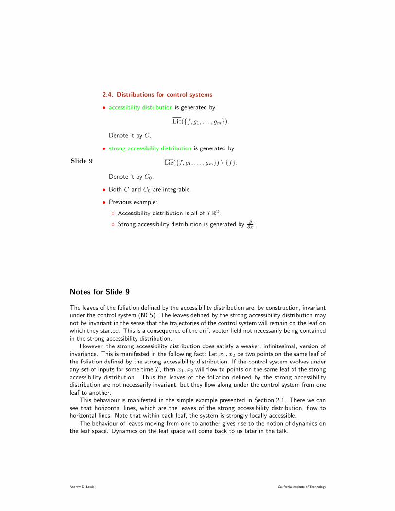
2.4. Distributions for control systems

• accessibility distribution is generated by

Lie(f, g1, . . . , gm).

Denote it by C.

• strong accessibility distribution is generated by

Lie(f, g1, . . . , gm) \ f.

Denote it by C0.

• Both C and C0 are integrable.

• Previous example:

Accessibility distribution is all of TR2.

Strong accessibility distribution is generated by ∂∂x

.

Notes for Slide 9

The leaves of the foliation defined by the accessibility distribution are, by construction, invariantunder the control system (NCS). The leaves defined by the strong accessibility distribution maynot be invariant in the sense that the trajectories of the control system will remain on the leaf onwhich they started. This is a consequence of the drift vector field not necessarily being containedin the strong accessibility distribution.

However, the strong accessibility distribution does satisfy a weaker, infinitesimal, version ofinvariance. This is manifested in the following fact: Let x1, x2 be two points on the same leaf ofthe foliation defined by the strong accessibility distribution. If the control system evolves underany set of inputs for some time T , then x1, x2 will flow to points on the same leaf of the strongaccessibility distribution. Thus the leaves of the foliation defined by the strong accessibilitydistribution are not necessarily invariant, but they flow along under the control system from oneleaf to another.

This behaviour is manifested in the simple example presented in Section 2.1. There we cansee that horizontal lines, which are the leaves of the strong accessibility distribution, flow tohorizontal lines. Note that within each leaf, the system is strongly locally accessible.

The behaviour of leaves moving from one to another gives rise to the notion of dynamics onthe leaf space. Dynamics on the leaf space will come back to us later in the talk.


Slide 10

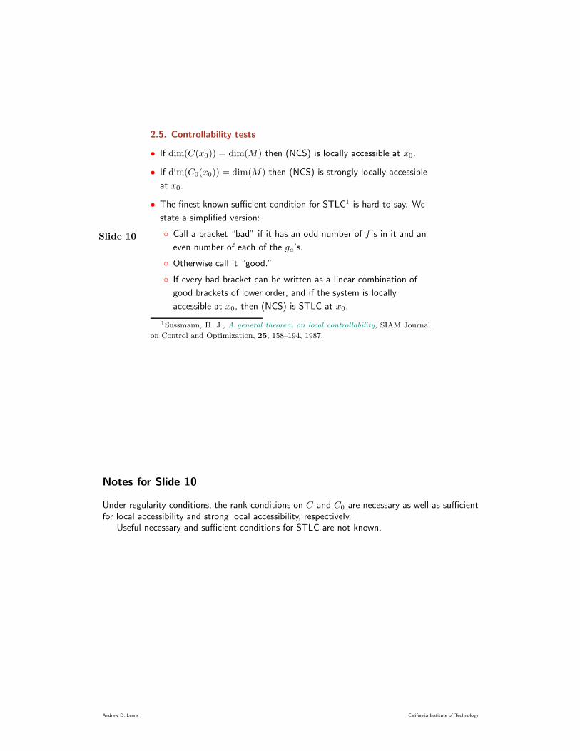
2.5. Controllability tests

• If dim(C(x0)) = dim(M) then (NCS) is locally accessible at x0.

• If dim(C0(x0)) = dim(M) then (NCS) is strongly locally accessible

at x0.

• The finest known sufficient condition for STLC1 is hard to say. We

state a simplified version:

Call a bracket “bad” if it has an odd number of f ’s in it and an

even number of each of the ga’s.

Otherwise call it “good.”

If every bad bracket can be written as a linear combination of

good brackets of lower order, and if the system is locally

accessible at x0, then (NCS) is STLC at x0.

1Sussmann, H. J., A general theorem on local controllability, SIAM Journal

on Control and Optimization, 25, 158–194, 1987.

Notes for Slide 10

Under regularity conditions, the rank conditions on C and C0 are necessary as well as sufficientfor local accessibility and strong local accessibility, respectively.

Useful necessary and sufficient conditions for STLC are not known.


Slide 11

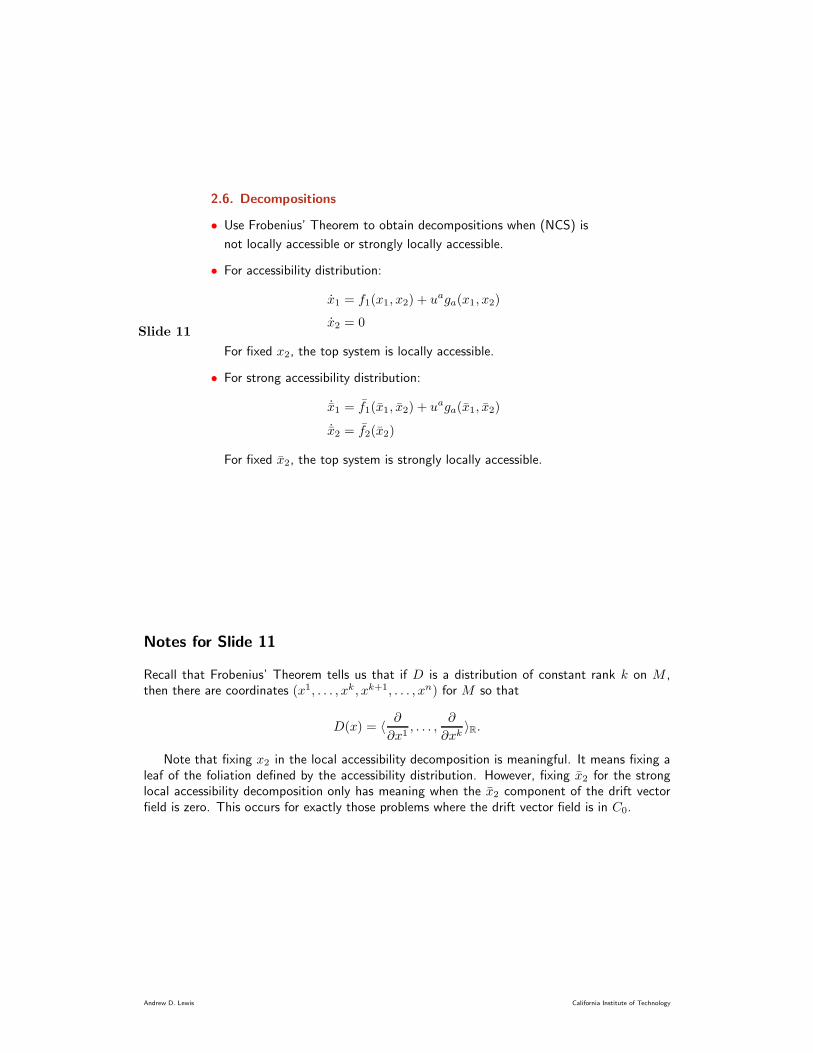
2.6. Decompositions

• Use Frobenius’ Theorem to obtain decompositions when (NCS) is

not locally accessible or strongly locally accessible.

• For accessibility distribution:

x1 = f1(x1, x2) + uaga(x1, x2)

x2 = 0

For fixed x2, the top system is locally accessible.

• For strong accessibility distribution:

˙x1 = f1(x1, x2) + uaga(x1, x2)

˙x2 = f2(x2)

For fixed x2, the top system is strongly locally accessible.

Notes for Slide 11

Recall that Frobenius’ Theorem tells us that if D is a distribution of constant rank k on M ,then there are coordinates (x1, . . . , xk, xk+1, . . . , xn) for M so that

D(x) = 〈∂

∂x1, . . . ,

∂

∂xk〉R.

Note that fixing x2 in the local accessibility decomposition is meaningful. It means fixing aleaf of the foliation defined by the accessibility distribution. However, fixing x2 for the stronglocal accessibility decomposition only has meaning when the x2 component of the drift vectorfield is zero. This occurs for exactly those problems where the drift vector field is in C0.


Slide 12

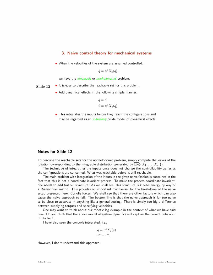
3. Naive control theory for mechanical systems

• When the velocities of the system are assumed controlled:

q = uaXa(q),

we have the kinematic or nonholonomic problem.

• It is easy to describe the reachable set for this problem.

• Add dynamical effects in the following simple manner:

q = v

v = uaXa(q).

• This integrates the inputs before they reach the configurations and

may be regarded as an extremely crude model of dynamical effects.

Notes for Slide 12

To describe the reachable sets for the nonholonomic problem, simply compute the leaves of thefoliation corresponding to the integrable distribution generated by Lie(X1, . . . , Xm).

The technique of integrating the inputs once does not change the controllability as far asthe configurations are concerned. What was reachable before is still reachable.

The main problem with integration of the inputs in the given naive fashion is contained in thefact that this is not a coordinate invariant process. To make the process coordinate invariant,one needs to add further structure. As we shall see, this structure is kinetic energy by way ofa Riemannian metric. This provides an important mechanism for the breakdown of the naivesetup presented here: Coriolis forces. We shall see that there are other factors which can alsocause the naive approach to fail. The bottom line is that the naive approach is far too naiveto be close to accurate in anything like a general setting. There is simply too big a differencebetween supplying torques and specifying velocities.

One may want to think about our robotic leg example in the context of what we have saidhere. Do you think that the above model of system dynamics will capture the correct behaviourof the leg?

I have also seen the controls integrated, i.e.,

q = vaXa(q)

va = ua.

However, I don’t understand this approach.


Slide 13

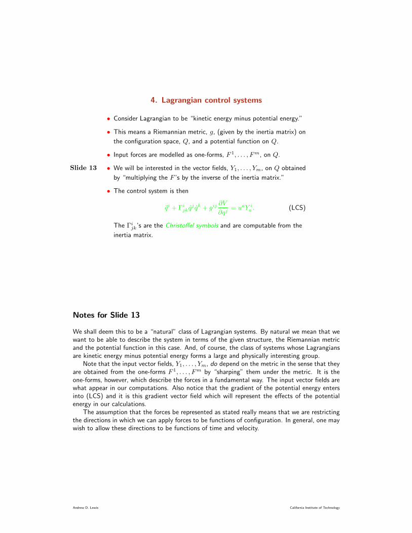
4. Lagrangian control systems

• Consider Lagrangian to be “kinetic energy minus potential energy.”

• This means a Riemannian metric, g, (given by the inertia matrix) on

the configuration space, Q, and a potential function on Q.

• Input forces are modelled as one-forms, F 1, . . . , Fm, on Q.

• We will be interested in the vector fields, Y1, . . . , Ym, on Q obtained

by “multiplying the F ’s by the inverse of the inertia matrix.”

• The control system is then

qi + Γijk qj qk + gij

∂V

∂qj= uaY ia . (LCS)

The Γijk’s are the Christoffel symbols and are computable from the

inertia matrix.

Notes for Slide 13

We shall deem this to be a “natural” class of Lagrangian systems. By natural we mean that wewant to be able to describe the system in terms of the given structure, the Riemannian metricand the potential function in this case. And, of course, the class of systems whose Lagrangiansare kinetic energy minus potential energy forms a large and physically interesting group.

Note that the input vector fields, Y1, . . . , Ym, do depend on the metric in the sense that theyare obtained from the one-forms F 1, . . . , Fm by “sharping” them under the metric. It is theone-forms, however, which describe the forces in a fundamental way. The input vector fields arewhat appear in our computations. Also notice that the gradient of the potential energy entersinto (LCS) and it is this gradient vector field which will represent the effects of the potentialenergy in our calculations.

The assumption that the forces be represented as stated really means that we are restrictingthe directions in which we can apply forces to be functions of configuration. In general, one maywish to allow these directions to be functions of time and velocity.


Slide 14

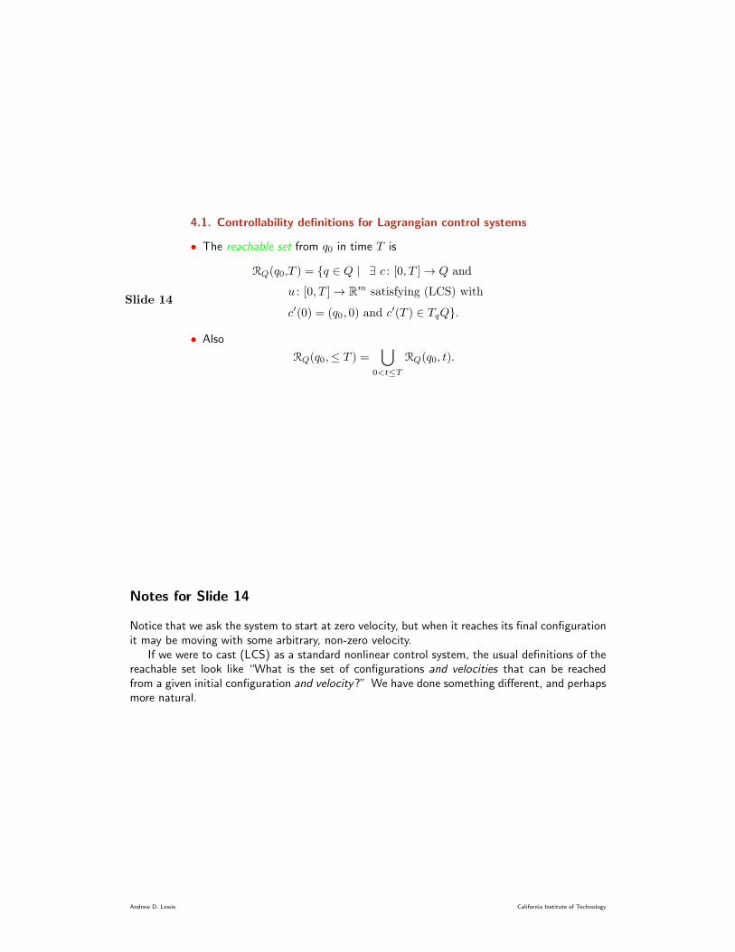
4.1. Controllability definitions for Lagrangian control systems

• The reachable set from q0 in time T is

RQ(q0,T ) = q ∈ Q | ∃ c : [0, T ] → Q and

u : [0, T ] → Rm satisfying (LCS) with

c′(0) = (q0, 0) and c′(T ) ∈ TqQ.

• Also

RQ(q0,≤ T ) =⋃

0<t≤T

RQ(q0, t).

Notes for Slide 14

Notice that we ask the system to start at zero velocity, but when it reaches its final configurationit may be moving with some arbitrary, non-zero velocity.

If we were to cast (LCS) as a standard nonlinear control system, the usual definitions of thereachable set look like “What is the set of configurations and velocities that can be reachedfrom a given initial configuration and velocity?” We have done something different, and perhapsmore natural.


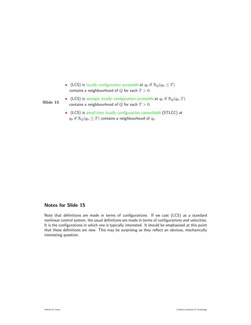
Slide 15

• (LCS) is locally configuration accessible at q0 if RQ(q0,≤ T )

contains a neighbourhood of Q for each T > 0.

• (LCS) is strongly locally configuration accessible at q0 if RQ(q0, T )

contains a neighbourhood of Q for each T > 0.

• (LCS) is small-time locally configuration controllable (STLCC) at

q0 if RQ(q0,≤ T ) contains a neighbourhood of q0.

Notes for Slide 15

Note that definitions are made in terms of configurations. If we cast (LCS) as a standardnonlinear control system, the usual definitions are made in terms of configurations and velocities.It is the configurations in which one is typically interested. It should be emphasised at this pointthat these definitions are new. This may be surprising as they reflect an obvious, mechanicallyinteresting question.


Slide 16

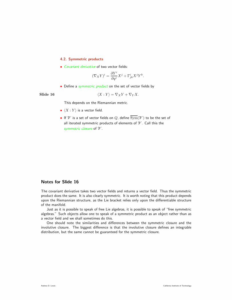
4.2. Symmetric products

• Covariant derivative of two vector fields:

(∇XY )i =∂Y i

∂qjXj + ΓijkX

jY k.

• Define a symmetric product on the set of vector fields by

〈X : Y 〉 = ∇XY +∇YX.

This depends on the Riemannian metric.

• 〈X : Y 〉 is a vector field.

• If V is a set of vector fields on Q, define Sym(V) to be the set of

all iterated symmetric products of elements of V. Call this the

symmetric closure of V.

Notes for Slide 16

The covariant derivative takes two vector fields and returns a vector field. Thus the symmetricproduct does the same. It is also clearly symmetric. It is worth noting that this product dependsupon the Riemannian structure, as the Lie bracket relies only upon the differentiable structureof the manifold.

Just as it is possible to speak of free Lie algebras, it is possible to speak of “free symmetricalgebras.” Such objects allow one to speak of a symmetric product as an object rather than asa vector field and we shall sometimes do this.

One should note the similarities and differences between the symmetric closure and theinvolutive closure. The biggest difference is that the involutive closure defines an integrabledistribution, but the same cannot be guaranteed for the symmetric closure.


Slide 17

4.3. Distributions of symmetric products and Lie brackets

• We wish to compute the accessibility distribution, C, at points of

zero velocity, denoted (q, 0).

• At (q, 0) define horizontal to be in the “q-direction” and vertical to

be in the “v-direction.”

Notes for Slide 17

The reason that we are interested in the accessibility distribution at points of zero velocity is thatthese are the initial conditions in our versions of controllability. Thus the distribution evaluatedat these points will be tangent to the reachable set.

We shall describe the accessibility distribution in terms of two distributions on Q. Onedistribution will represent the vertical directions in the figure, and the other the horizontaldirections.

Please note that the decomposition into horizontal and vertical as described above does not,in general, make sense except at points where the velocity is zero. Other decompositions maybe made at points of non-zero velocity, but we shall not go into that here.


Slide 18

• Denote Y = Y1, . . . , Ym.

• All vertical directions for C are generated by R-linear combinations

of vector fields from Sym(Y ∪ gradV ).

• All horizontal directions for C are generated by R-linear

combinations of vector fields from Lie(Sym(Y ∪ gradV )).

• An algorithm determines which R-linear combinations to choose.

• Define two distributions on Q,

Cver(Y, V ),

Chor(Y, V )

as the vertical and horizontal directions, respectively, for C.

Notes for Slide 18

Although we have an algorithm for computing which vector fields from Sym(Y ∪ gradV )and Lie(Sym(Y ∪ gradV )) are present in the accessibility distribution, it would be nice tocompute an inductive formula for these vector fields. This seems to be quite difficult.


Slide 19

• It is easy to show that Chor(Y, V ) is an integrable distribution.

• Special Case of V = 0:

The vertical directions are generated by Sym(Y).

The horizontal directions are generated by Lie(Sym(Y)).

Cver(Y, V ) ⊂ Chor(Y, V ).

Notes for Slide 19

The integrability of Chor(Y, V ) is important in our decompositions we state later.The fact that Cver(Y, V ) ⊂ Chor(Y, V ) means that solutions starting with zero velocity

will remain on leaves of the foliation defined by Chor(Y, V ). Note that this only happens ingeneral if V = 0. There are other special cases when the solutions will remain on the leaves ofChor(Y, V ). This is discussed further when we present decompositions for Lagrangian controlsystems.


Slide 20

4.4. Controllability tests for mechanical control systems

• If dim(Chor(Y, V )(q0)) = dim(Q) then (LCS) is locally

configuration accessible at q0.

• Conditions for STLCC are similar to those for STLC in (NCS).

We shall call a symmetric product in Sym(Y ∪ gradV ) “bad”

if the number of times that each vector field Ya appears is even.

Otherwise the symmetric product is called “good.”

If each bad symmetric product can be written as a linear

combination of good symmetric products of lower order, and if

the system is locally configuration accessible at q0, then (LCS) is

STLCC at q0.

Notes for Slide 20

Notice that we do not bother with strong local configuration accessibility. This is somethingthat we would like to understand better.

The conditions for STLCC actually give more than is implied. It is, in fact, possible to gofrom a configuration q0 at rest to a neighbourhood of q0 at rest. This allows us to define thenotion of “equilibrium controllability” whereby one can steer between two equilibrium points atrest.


Slide 21

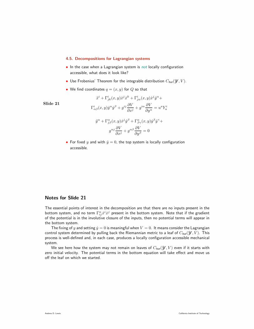
4.5. Decompositions for Lagrangian systems

• In the case when a Lagrangian system is not locally configuration

accessible, what does it look like?

• Use Frobenius’ Theorem for the integrable distribution Chor(Y, V ).

• We find coordinates q = (x, y) for Q so that

xi + Γijk(x, y)xj xk + Γijα(x, y)x

j yα+

Γiαβ(x, y)yαyβ + gij

∂V

∂xj+ giα

∂V

∂yα= uaY ia

yα + Γαjβ(x, y)xj yβ + Γαβγ(x, y)y

β yγ+

gαj∂V

∂xj+ gαβ

∂V

∂yβ= 0

• For fixed y and with y = 0, the top system is locally configuration

accessible.

Notes for Slide 21

The essential points of interest in the decomposition are that there are no inputs present in thebottom system, and no term Γαij x

ixj present in the bottom system. Note that if the gradientof the potential is in the involutive closure of the inputs, then no potential terms will appear inthe bottom system.

The fixing of y and setting y = 0 is meaningful when V = 0. It means consider the Lagrangiancontrol system determined by pulling back the Riemannian metric to a leaf of Chor(Y, V ). Thisprocess is well-defined and, in each case, produces a locally configuration accessible mechanicalsystem.

We see here how the system may not remain on leaves of Chor(Y, V ) even if it starts withzero initial velocity. The potential terms in the bottom equation will take effect and move usoff the leaf on which we started.


Slide 22

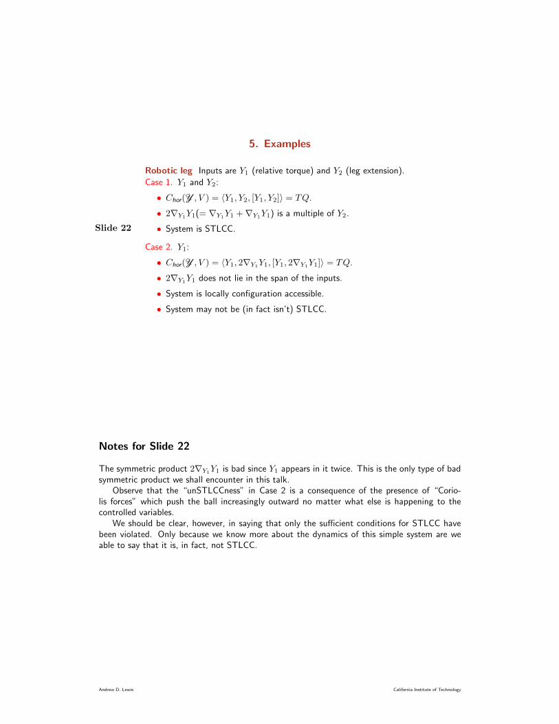
5. Examples

Robotic leg Inputs are Y1 (relative torque) and Y2 (leg extension).

Case 1. Y1 and Y2:

• Chor(Y, V ) = 〈Y1, Y2, [Y1, Y2]〉 = TQ.

• 2∇Y1Y1(= ∇Y1

Y1 +∇Y1Y1) is a multiple of Y2.

• System is STLCC.

Case 2. Y1:

• Chor(Y, V ) = 〈Y1, 2∇Y1Y1, [Y1, 2∇Y1

Y1]〉 = TQ.

• 2∇Y1Y1 does not lie in the span of the inputs.

• System is locally configuration accessible.

• System may not be (in fact isn’t) STLCC.

Notes for Slide 22

The symmetric product 2∇Y1Y1 is bad since Y1 appears in it twice. This is the only type of bad

symmetric product we shall encounter in this talk.Observe that the “unSTLCCness” in Case 2 is a consequence of the presence of “Corio-

lis forces” which push the ball increasingly outward no matter what else is happening to thecontrolled variables.

We should be clear, however, in saying that only the sufficient conditions for STLCC havebeen violated. Only because we know more about the dynamics of this simple system are weable to say that it is, in fact, not STLCC.


Slide 23

Case 3. Y2:

• Chor(Y, V ) = 〈Y2〉 ( TQ.

• System is not locally configuration accessible.

• The local configuration accessibility decomposition of the system

is given by

r − rψ2 =1

mu1

θ = 0

ψ +2

rrψ = 0.

Notes for Slide 23

The readers should assure themselves that the decomposition has the advertised properties: Noinputs appear in the bottom system and there are no terms quadratic in r in the bottom system.In this case, since the potential energy is zero, this means that θ and ψ remain at their initialvalues if θ(0) and ψ(0) are both zero.


Slide 24

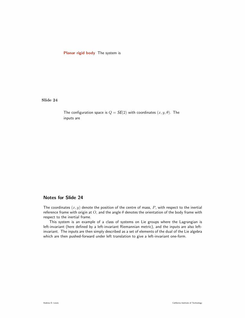
Planar rigid body The system is

The configuration space is Q = SE(2) with coordinates (x, y, θ). The

inputs are

Notes for Slide 24

The coordinates (x, y) denote the position of the centre of mass, P , with respect to the inertialreference frame with origin at O, and the angle θ denotes the orientation of the body frame withrespect to the inertial frame.

This system is an example of a class of systems on Lie groups where the Lagrangian isleft-invariant (here defined by a left-invariant Riemannian metric), and the inputs are also left-invariant. The inputs are then simply described as a set of elements of the dual of the Lie algebrawhich are then pushed-forward under left translation to give a left-invariant one-form.


Slide 25

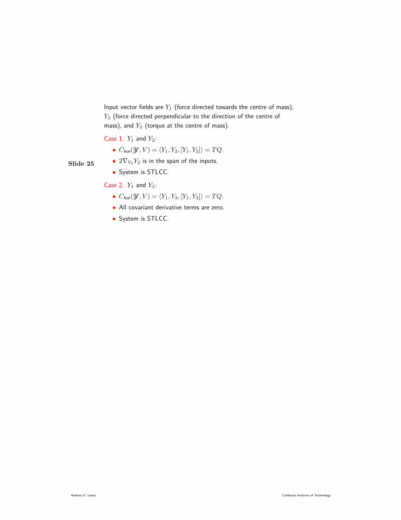
Input vector fields are Y1 (force directed towards the centre of mass),

Y2 (force directed perpendicular to the direction of the centre of

mass), and Y3 (torque at the centre of mass).

Case 1. Y1 and Y2:

• Chor(Y, V ) = 〈Y1, Y2, [Y1, Y2]〉 = TQ.

• 2∇Y2Y2 is in the span of the inputs.


Case 2. Y1 and Y3:

• Chor(Y, V ) = 〈Y1, Y3, [Y1, Y3]〉 = TQ.

• All covariant derivative terms are zero.



Slide 26

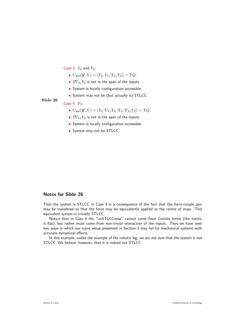
Case 3. Y2 and Y3:

• Chor(Y, V ) = 〈Y2, Y3, [Y2, Y3]〉 = TQ.

• 2∇Y2Y2 is not in the span of the inputs.


• System may not be (but actually is) STLCC.

Case 4. Y2:

• Chor(Y, V ) = 〈Y2,∇Y2Y2, [Y2,∇Y2

Y2]〉 = TQ.

• 2∇Y2Y2 is not in the span of the inputs.


• System may not be STLCC.

Notes for Slide 26

That the system is STLCC in Case 3 is a consequence of the fact that the force-couple pairmay be transfered so that the force may be equivalently applied at the centre of mass. Thisequivalent system is trivially STLCC.

Notice that in Case 4 the “unSTLCCness” cannot come from Coriolis terms (the metricis flat), but rather must come from non-trivial interaction of the inputs. Thus we have seentwo ways in which our naive setup presented in Section 3 may fail for mechanical systems withaccurate dynamical effects.

In this example, unlike the example of the robotic leg, we are not sure that the system is notSTLCC. We believe, however, that it is indeed not STLCC.


Slide 27

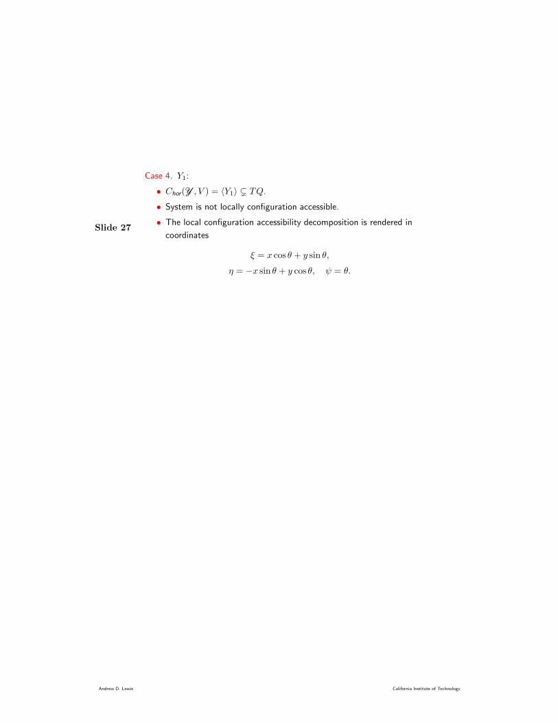
Case 4. Y1:

• Chor(Y, V ) = 〈Y1〉 ( TQ.

• System is not locally configuration accessible.

• The local configuration accessibility decomposition is rendered in

coordinates

ξ = x cos θ + y sin θ,

η = −x sin θ + y cos θ, ψ = θ.


Slide 28

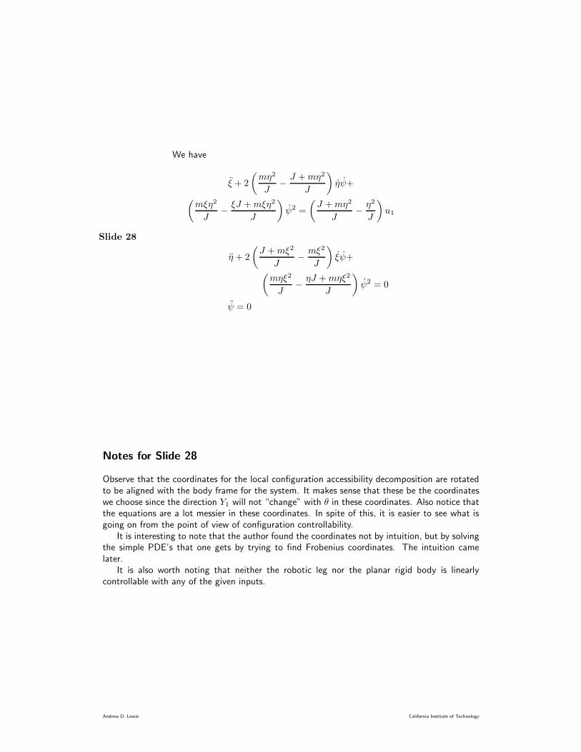
We have

ξ + 2

(

mη2

J−J +mη2

J

)

ηψ+

(

mξη2

J−ξJ +mξη2

J

)

ψ2 =

(

J +mη2

J−η2

J

)

u1

η + 2

(

J +mξ2

J−mξ2

J

)

ξψ+

(

mηξ2

J−ηJ +mηξ2

J

)

ψ2 = 0

ψ = 0

Notes for Slide 28

Observe that the coordinates for the local configuration accessibility decomposition are rotatedto be aligned with the body frame for the system. It makes sense that these be the coordinateswe choose since the direction Y1 will not “change” with θ in these coordinates. Also notice thatthe equations are a lot messier in these coordinates. In spite of this, it is easier to see what isgoing on from the point of view of configuration controllability.

It is interesting to note that the author found the coordinates not by intuition, but by solvingthe simple PDE’s that one gets by trying to find Frobenius coordinates. The intuition camelater.

It is also worth noting that neither the robotic leg nor the planar rigid body is linearlycontrollable with any of the given inputs.


Slide 29

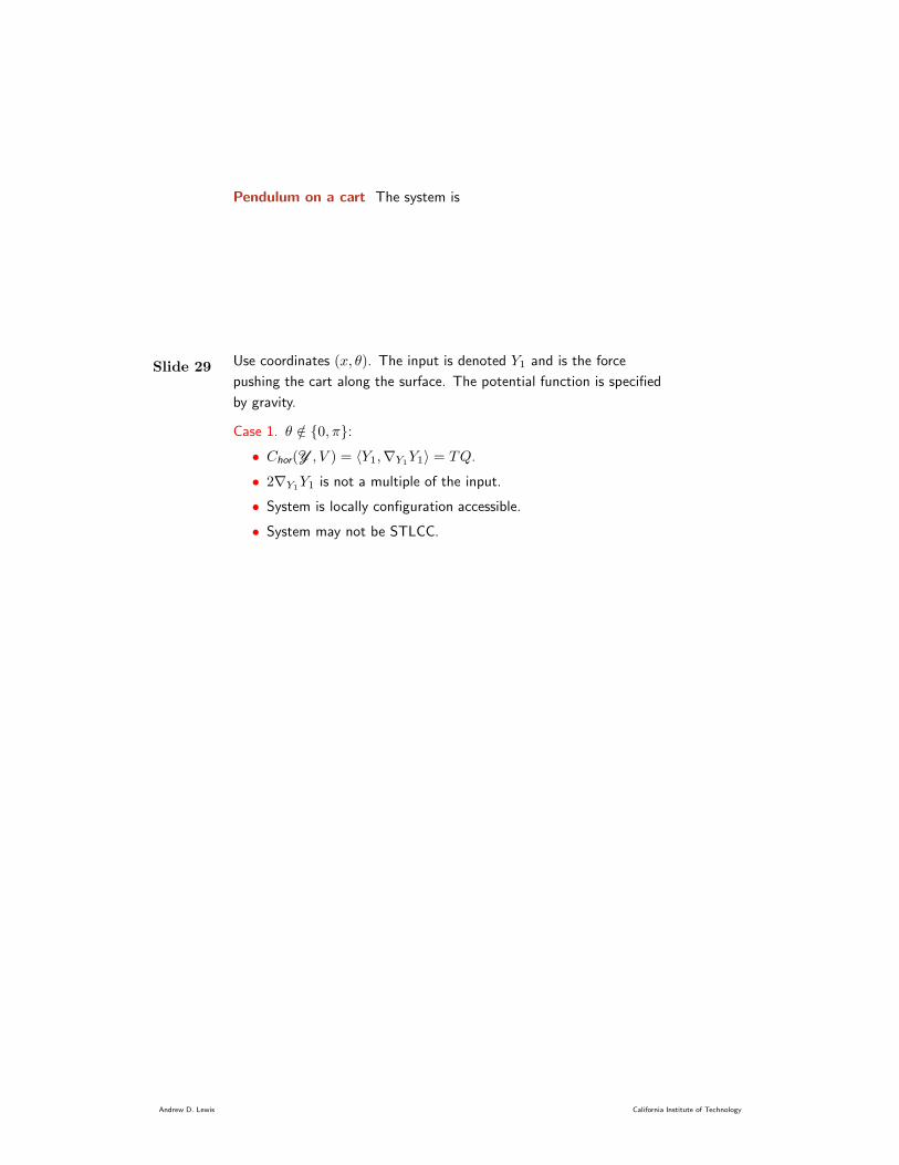
Pendulum on a cart The system is

Use coordinates (x, θ). The input is denoted Y1 and is the force

pushing the cart along the surface. The potential function is specified

by gravity.

Case 1. θ /∈ 0, π:

• Chor(Y, V ) = 〈Y1,∇Y1Y1〉 = TQ.

• 2∇Y1Y1 is not a multiple of the input.


• System may not be STLCC.


Slide 30

Case 2. θ ∈ 0, π:

• Chor(Y, V ) = 〈Y1,∇gradV Y1 +∇Y1gradV 〉 = TQ.

• 2∇Y1Y1 = 0.


Notes for Slide 30

At the points where θ ∈ 0, π, the linearisation is controllable so it must be that the nonlinearsystem is STLC, and hence STLCC.


Slide 31

5.1. Wrap up for Lagrangian control theory

• Conclusions:

New and meaningful definitions of controllability for simple

mechanical control systems.

Computable conditions for these new notions of controllability in

terms of data defined on Q.

Surprising geometric insight.

• Future explorations:

Why covariant derivatives?

Find a smaller generating set.

What about non-zero initial velocities?

More general Lagrangians.

Better conditions for STLCC.

Synthesis.

Notes for Slide 31

It cannot be emphasised enough that the definitions for controllability we present, while naturalenough, have not appeared in the literature. This is especially interesting as we are able to derivefairly nice conditions for checking these definitions of controllability.

We say that the geometric insights gained by this work are surprising since the appearanceof the covariant derivative is not something which was expected at the outset. Although wehave seen a little of what the covariant derivative terms give us with the centrifugal effects inthe robotic leg, we still do not fully understand why they are present.

Notice that in the definitions of Cver(Y, V ) and Chor(Y, V ), we added all covariant deriva-tives and Lie brackets. In fact we do not need all of them since they will not be linearlyindependent in general. It would be helpful to determine a way of computing a generating setwhich requires the computation of fewer covariant derivatives and Lie brackets. This is relatedto finding Philip Hall bases for free Lie algebras.


Slide 32

6. Hamiltonian control systems

• A Hamiltonian system is specified by a Hamiltonian function (plus

things described later) which is the energy of the system.

• A Hamiltonian control system is specified by the system

Hamiltonian H0 plus control Hamiltonians, H1, . . . , Hm.

• Associated with a Hamiltonian function H is the Hamiltonian vector

field XH . A Hamiltonian control system has the form

x = XH0+ uaXHa

. (HCS)

Notes for Slide 32

As with Lagrangian systems, we choose a “natural” structure for Hamiltonian control systems.While it is fairly clear that the Lagrangian setup represents a lot of interesting systems, the samecannot so easily be said of the Hamiltonian control framework we present. It is, however, truethat a lot of systems fall into the given framework, at least locally. The reason for this is that,for many systems, the control Hamiltonians are simply coordinate functions in some chart andso the corresponding vector field is, by construction, locally Hamiltonian. The global issues ofthis vector field not being properly Hamiltonian are not so important to us since we are in thebusiness of presenting local decomposition theorems.


Slide 33

6.1. Geometry of Hamiltonian systems (Poisson manifolds)

• The general setting for Hamiltonian mechanics is a Poisson

manifold.

• A Poisson manifold may (loosely) be characterised as a manifold

having local coordinates (q1, . . . , qn, p1, . . . , pn, c1, . . . , cs) so that

the Hamiltonian vector field with Hamiltonian H is given by

qi =∂H

∂pi

pi = −∂H

∂qi

ca = 0

• The surfaces defined by ca = const . are invariant under all

Hamiltonian vector fields.

• A Poisson manifold P is symplectic if dim(P ) = 2n. Thus a

symplectic manifold is a “nondegenerate” Poisson manifold.

Notes for Slide 33

Our “definition” of a Poisson manifold is backwards. The real definition defines a tensor field onP of a certain type. With this structure, one may move on to define Hamiltonian vector fields.However, the picture of a Poisson manifold being the disjoint union of a bunch of symplecticmanifolds is a general one.

When we define a Hamiltonian control system we shall assume that it evolves on a symplectic

manifold. Poisson manifolds come up later in the analysis.


Slide 34

6.2. Decompositions for Hamiltonian control systems

• Let C be the accessibility distribution and let C0 be the strong

accessibility distribution. Denote the corresponding foliations by FC

and FC0.

• Study dynamics on the leaves and on the leaf space.

• On each leaf of FC the symplectic structure is degenerate.

“Quotienting out” the degeneracy gives a “reduced” symplectic

manifold.

• The system (HCS) drops to this reduced manifold and there gives a

locally accessible Hamiltonian control system.

• There is one such reduced control system for each leaf of FC .

• The reduced dynamics may be regarded as the “locally accessible

dynamics.”

Notes for Slide 34

The distributions C and C0 are computed in the usual manner described above for generalnonlinear systems. Because the drift and control vector fields are Hamiltonian, there is a lot ofstructure to their involutive closure.

This “quotienting out” procedure is very much the same as the reduction of the level sets ofthe momentum map in classical Hamiltonian reduction. In fact, in many examples it is exactlythis procedure: the control system leaves some conservation law undisturbed and so restricts tothe level sets of the conserved quantities. The reduction then follows the classical methods.

Observe that we get many sets of locally accessible dynamics, one for each leaf of FC .


Slide 35

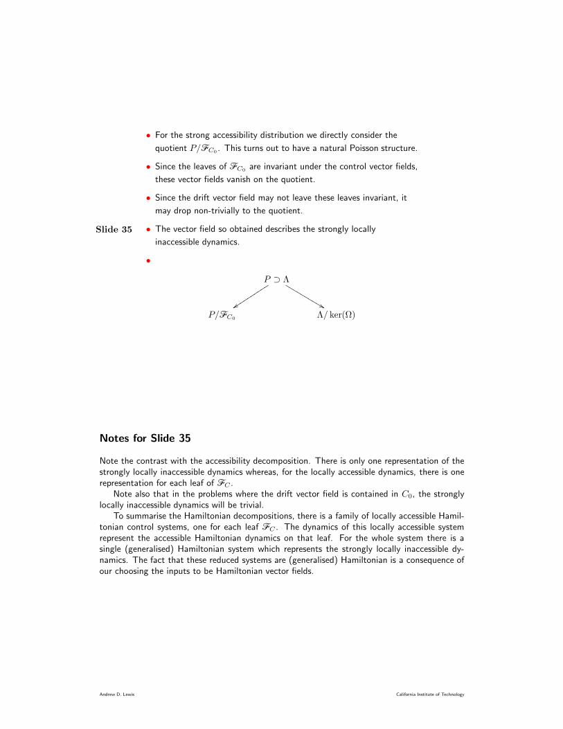
• For the strong accessibility distribution we directly consider the

quotient P/FC0. This turns out to have a natural Poisson structure.

• Since the leaves of FC0are invariant under the control vector fields,

these vector fields vanish on the quotient.

• Since the drift vector field may not leave these leaves invariant, it

may drop non-trivially to the quotient.

• The vector field so obtained describes the strongly locally

inaccessible dynamics.

•

P ⊃ Λ

yytttttttttt

&&

P/FC0Λ/ ker(Ω)

Notes for Slide 35

Note the contrast with the accessibility decomposition. There is only one representation of thestrongly locally inaccessible dynamics whereas, for the locally accessible dynamics, there is onerepresentation for each leaf of FC .

Note also that in the problems where the drift vector field is contained in C0, the stronglylocally inaccessible dynamics will be trivial.

To summarise the Hamiltonian decompositions, there is a family of locally accessible Hamil-tonian control systems, one for each leaf FC . The dynamics of this locally accessible systemrepresent the accessible Hamiltonian dynamics on that leaf. For the whole system there is asingle (generalised) Hamiltonian system which represents the strongly locally inaccessible dy-namics. The fact that these reduced systems are (generalised) Hamiltonian is a consequence ofour choosing the inputs to be Hamiltonian vector fields.


Slide 36

The examples as Hamiltonian control systems

Robotic leg with both inputs

• Hamiltonian is

H =1

2Jp2θ +

1

2m

(

p2r + r−2p2ψ)

.

• Control Hamiltonians are H1 = θ − ψ and H2 = r.

• Leaves of C are given by ang. mom. = pθ + pψ = const . = µ.

• Reduced manifold is described by coordinates

(r, φ = θ − ψ, pr, pφ = pθ − pψ).

Notes for Slide 36

The calculations for Hamiltonian control systems need much more information than we havepresented here. Therefore, we shall present just the “answers” and not go into how to computethem in any detail.

Note that θ − ψ is not really a function on Q and so XH1is only locally Hamiltonian.

The reduced control system lives on T ∗(S1×R) with its canonical symplectic structure. Onecan obtain this reduction by classical methods of group reduction.


Slide 37

• Reduced Hamiltonian is

Hµ =1

2mp2r +

(

1

8J+

1

8mr2

)

p2φ+

(

1

4mr2−

1

4J

)

µpφ +

(

1

8J+

1

8mr2

)

µ2.

• Reduced control Hamiltonians are H1,µ = φ and H2,µ = 0.

• Strongly inaccessible dynamics are trivial.

Robotic leg with torque between bodies

• Same as both inputs.

Notes for Slide 37

It may be verified that the Hamiltonian control system on T ∗(S1×R) with Hamiltonian Hµ andcontrol Hamiltonian H1,µ is indeed locally accessible.


Slide 38

Robotic leg with leg extension

• Leaves of C are given by pθ = const . = µ and pψ = const . = ν.

• Reduced manifold is described by coordinates (r, pr).

• Reduced Hamiltonian is

Hµ,ν =1

2mp2r +

1

2mr2ν2 +

1

2Jµ2.

• Reduced control Hamiltonian is H2,µ,ν = r.

• The strongly inaccessible dynamics live on a Poisson manifold with

coordinates (θ, pθ, pψ).

• The Hamiltonian is H =1

2Jp2θ.

Notes for Slide 38

In this case, the angular momentum of the body and of the leg are both conserved by the input.For the other inputs, only their sum is conserved. The reduction in the case of the leg extensioninput can also be accomplished using group methods, this time with the group T2.

The coordinates (θ, pθ, pψ) are coordinates for a Poisson manifold where q1 = θ, p1 = pθ,and c1 = pψ. The strongly locally inaccessible dynamics represent the fact that, with this input,the rigid body part of the system moves unaffected by the inputs.


Slide 39

Planar rigid body

• Cannot be represented as a Hamiltonian control system.

Pendulum on a cart

• Can be represented as a Hamiltonian control system but it is trivial

since the system is strongly locally accessible.

Notes for Slide 39

The planar rigid body cannot be represented as a Hamiltonian control system since the inputvector fields Y1 and Y2 are not even locally Hamiltonian. The vector field Y3 is locally Hamiltonianso the system can be locally represented as a Hamiltonian system with only this input. But thisis the most uninteresting input.

For the pendulum on the cart, the system is strongly locally accessible so the locally accessibledynamics are the original dynamics and the strongly locally inaccessible dynamics are trivial.


Slide 40

6.3. Wrap up for Hamiltonian control theory

• Conclusions:

The “controllable” dynamics are Hamiltonian.

The “uncontrollable” dynamics are Hamiltonian.

• Future explorations:

Make connections with Lagrangian results.

More general inputs.

Notes for Slide 40

Although this Hamiltonian picture is very attractive, it may not offer so much from a practicalviewpoint. The first restriction is that it needs input vector fields which are Hamiltonian. Thisis a large restriction. If this could be fixed up somehow it would be very interesting. Also,for Hamiltonian control systems on cotangent bundles, this presentation does not address theimportant mechanical issues, some of which are touched upon in the Lagrangian control theorywe presented.


Documents

Controllability mechanical control systems - mast.queensu.caandrew/talks/pdf/1995a.pdfSlide0 Controllability of mechanical control systems Andrew D. Lewis∗ 21/04/1995 ∗Advisor: