Embed Size (px)
Citation preview
The Bloch equationLinearized system
Non exact controllability with a priori bounded controlsApproximate controllability with unbounded controls
Explicit controls for the asymptotic exact controllabilityFeedback stabilization
Control and stabilization of the Bloch equation
Karine Beauchard (CNRS, CMLS, Ecole Polytechnique)
joint works with
Jean-Michel Coron (LJLL, Paris 6)
Pierre Rouchon (CAS, Mines de Paris)
Paulo Sergio Pereira da Silva (Escola Politecnica Sao Polo)
QUAINT, Dijon, April, 9, 2013K. Beauchard
The Bloch equationLinearized system
Non exact controllability with a priori bounded controlsApproximate controllability with unbounded controls
Explicit controls for the asymptotic exact controllabilityFeedback stabilization
Plan
1 The Bloch equation
2 Linearized system
3 Non exact controllability with a priori bounded controls
4 Approximate controllability with unbounded controls
5 Explicit controls for the asymptotic exact controllability
6 Feedback stabilization
K. Beauchard
The Bloch equationLinearized system
Non exact controllability with a priori bounded controlsApproximate controllability with unbounded controls
Explicit controls for the asymptotic exact controllabilityFeedback stabilization
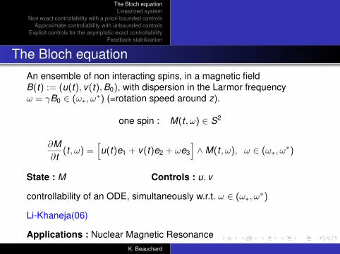
The Bloch equationAn ensemble of non interacting spins, in a magnetic fieldB(t) := (u(t), v(t),B0), with dispersion in the Larmor frequencyω = γB0 ∈ (ω∗, ω
∗) (=rotation speed around z).
one spin : M(t , ω) ∈ S2
∂M∂t
(t , ω) =[u(t)e1 + v(t)e2 + ωe3
]∧M(t , ω), ω ∈ (ω∗, ω
∗)
State : M Controls : u, v
controllability of an ODE, simultaneously w.r.t. ω ∈ (ω∗, ω∗)
Li-Khaneja(06)
Applications : Nuclear Magnetic ResonanceK. Beauchard
The Bloch equationLinearized system
Non exact controllability with a priori bounded controlsApproximate controllability with unbounded controls
Explicit controls for the asymptotic exact controllabilityFeedback stabilization
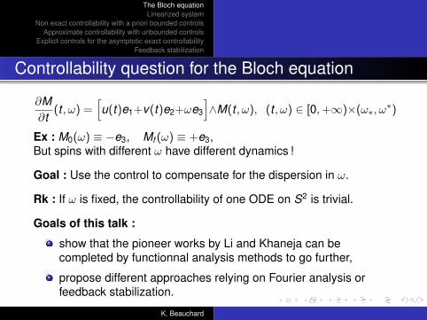
Controllability question for the Bloch equation
∂M∂t
(t , ω) =[u(t)e1+v(t)e2+ωe3
]∧M(t , ω), (t , ω) ∈ [0,+∞)×(ω∗, ω
∗)
Ex : M0(ω) ≡ −e3, Mf (ω) ≡ +e3,But spins with different ω have different dynamics !
Goal : Use the control to compensate for the dispersion in ω.
Rk : If ω is fixed, the controllability of one ODE on S2 is trivial.
Goals of this talk :
show that the pioneer works by Li and Khaneja can becompleted by functionnal analysis methods to go further,
propose different approaches relying on Fourier analysis orfeedback stabilization.
K. Beauchard
The Bloch equationLinearized system
Non exact controllability with a priori bounded controlsApproximate controllability with unbounded controls
Explicit controls for the asymptotic exact controllabilityFeedback stabilization
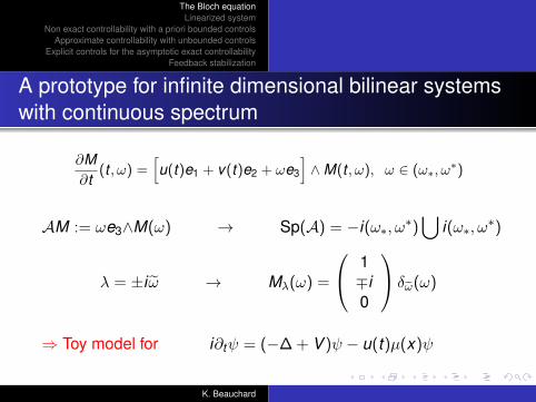
A prototype for infinite dimensional bilinear systemswith continuous spectrum
∂M∂t
(t , ω) =[u(t)e1 + v(t)e2 + ωe3
]∧M(t , ω), ω ∈ (ω∗, ω
∗)
AM := ωe3∧M(ω) → Sp(A) = −i(ω∗, ω∗)⋃
i(ω∗, ω∗)
λ = ±iω → Mλ(ω) =
1∓i0
δω(ω)
⇒ Toy model for i∂tψ = (−∆ + V )ψ − u(t)µ(x)ψ
K. Beauchard
The Bloch equationLinearized system
Non exact controllability with a priori bounded controlsApproximate controllability with unbounded controls
Explicit controls for the asymptotic exact controllabilityFeedback stabilization
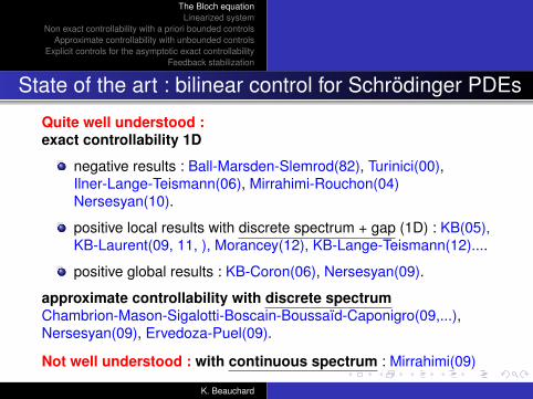
State of the art : bilinear control for Schrödinger PDEs
Quite well understood :exact controllability 1D
negative results : Ball-Marsden-Slemrod(82), Turinici(00),Ilner-Lange-Teismann(06), Mirrahimi-Rouchon(04)Nersesyan(10).
positive local results with discrete spectrum + gap (1D) : KB(05),KB-Laurent(09, 11, ), Morancey(12), KB-Lange-Teismann(12)....
positive global results : KB-Coron(06), Nersesyan(09).
approximate controllability with discrete spectrumChambrion-Mason-Sigalotti-Boscain-Boussaïd-Caponigro(09,...),Nersesyan(09), Ervedoza-Puel(09).
Not well understood : with continuous spectrum : Mirrahimi(09)
K. Beauchard
The Bloch equationLinearized system
Non exact controllability with a priori bounded controlsApproximate controllability with unbounded controls
Explicit controls for the asymptotic exact controllabilityFeedback stabilization
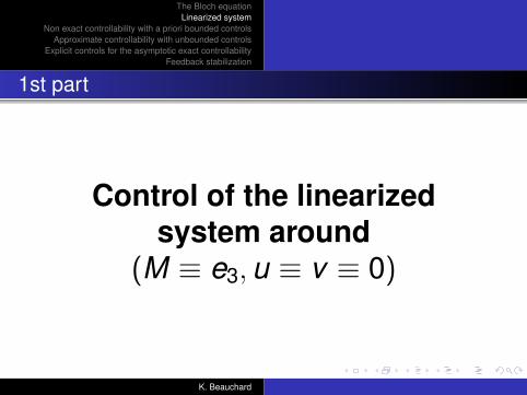
1st part
Control of the linearizedsystem around
(M ≡ e3,u ≡ v ≡ 0)
K. Beauchard
The Bloch equationLinearized system
Non exact controllability with a priori bounded controlsApproximate controllability with unbounded controls
Explicit controls for the asymptotic exact controllabilityFeedback stabilization
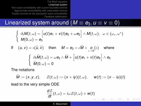
Linearized system around (M ≡ e3,u ≡ v ≡ 0)∂tM(t , ω) =
[u(t)e1 + v(t)e2 + ωe3
]∧M(t , ω), ω ∈ (ω∗, ω
∗)
M(0, ω) = e3
If (u, v) = ε(u, v) then M = e3 + εM + oε→0
(ε) where∂tM(t , ω) = ωe3 ∧ M +
[u(t)e1 + v(t)e2
]∧ e3
M(0, ω) = 0
The notations
M := (x , y , z), Z(t , ω) := (x + iy)(t , ω), w(t) := (v − iu)(t)
lead to the very simple ODE
dZdt
(t , ω) = iωZ(t , ω) + w(t)
K. Beauchard
The Bloch equationLinearized system
Non exact controllability with a priori bounded controlsApproximate controllability with unbounded controls
Explicit controls for the asymptotic exact controllabilityFeedback stabilization
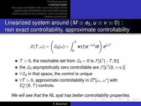
Linearized system around (M ≡ e3,u ≡ v ≡ 0) :non exact controllability, approximate controllability
Z(T , ω) =
(Z0(ω) +
∫ T
0w(t)e−iωtdt
)eiωT
T > 0, the reachable set from Z0 = 0 is F [L1(−T ,0)]
the Z0 asymptotically zero controllable are F [L1(0,+∞)]
∀Z0 in that space, the control is unique∀T > 0, approximate controllability in C0[ω∗, ω
∗] withC∞c (0,T )-controls.
We will see that the NL syst has better controllability properties.
K. Beauchard
The Bloch equationLinearized system
Non exact controllability with a priori bounded controlsApproximate controllability with unbounded controls
Explicit controls for the asymptotic exact controllabilityFeedback stabilization
2nd part
Nonlinear system :no exact controllability with a
priori bounded controls
K. Beauchard
The Bloch equationLinearized system
Non exact controllability with a priori bounded controlsApproximate controllability with unbounded controls
Explicit controls for the asymptotic exact controllabilityFeedback stabilization
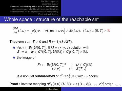
Whole space : structure of the reachable set
∂M∂t
(t , ω) =[u(t)e1 + v(t)e2 + ωe3
]∧M(t , ω), (t , ω) ∈ (0,T )× R
Theorem : Let T > 0 and R := 1/(8√
3T ).
∀u, v ∈ BR[L2(0,T )],∃!M = (x , y , z) solution withZ := x + iy ∈ C0([0,T ],L2(R)) ∩ C0
b ([0,T ]× R),
the image of
FT : BR[L2(0,T )]2 → L2 ∩ C0b (R)
(u, v) 7→ Z(T , .)
is a non flat submanifold of L2 ∩ C0b (R), with∞ codim.
Proof : Inverse mapping dFT (0,0).(U,V ) ∼ F(U + iV ) + 2nd orderK. Beauchard
The Bloch equationLinearized system
Non exact controllability with a priori bounded controlsApproximate controllability with unbounded controls
Explicit controls for the asymptotic exact controllabilityFeedback stabilization
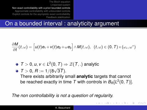
On a bounded interval : analyticity argument
∂M∂t
(t , ω) =[u(t)e1 +v(t)e2 +ωe3
]∧M(t , ω), (t , ω) ∈ (0,T )×(ω∗, ω
∗)
T > 0,u, v ∈ L2(0,T )⇒ Z(T , .) analyticT > 0, R := 1/(8
√3T ).
There exists arbitrarily small analytic targets that cannotbe reached exactly in time T with controls in BR[L2(0,T )].
The non controllability is not a question of regularity.
K. Beauchard
The Bloch equationLinearized system
Non exact controllability with a priori bounded controlsApproximate controllability with unbounded controls
Explicit controls for the asymptotic exact controllabilityFeedback stabilization
3rd part
Nonlinear system :approximate controllabilitywith unbounded controls
K. Beauchard
The Bloch equationLinearized system
Non exact controllability with a priori bounded controlsApproximate controllability with unbounded controls
Explicit controls for the asymptotic exact controllabilityFeedback stabilization
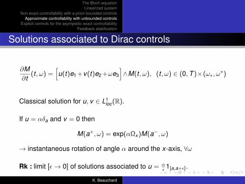
Solutions associated to Dirac controls
∂M∂t
(t , ω) =[u(t)e1 +v(t)e2 +ωe3
]∧M(t , ω), (t , ω) ∈ (0,T )×(ω∗, ω
∗)
Classical solution for u, v ∈ L1loc(R).
If u = αδa and v = 0 then
M(a+, ω) = exp(αΩx )M(a−, ω)
→ instantaneous rotation of angle α around the x-axis, ∀ω
Rk : limit [ε→ 0] of solutions associated to u = αε 1[a,a+ε].
K. Beauchard
The Bloch equationLinearized system
Non exact controllability with a priori bounded controlsApproximate controllability with unbounded controls
Explicit controls for the asymptotic exact controllabilityFeedback stabilization
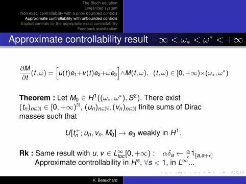
Approximate controllability result −∞ < ω∗ < ω∗ < +∞
∂M∂t
(t , ω) =[u(t)e1+v(t)e2+ωe3
]∧M(t , ω), (t , ω) ∈ [0,+∞)×(ω∗, ω
∗)
Theorem : Let M0 ∈ H1((ω∗, ω∗),S2). There exist
(tn)n∈N ∈ [0,+∞)N, (un)n∈N, (vn)n∈N finite sums of Diracmasses such that
U[t+n ; un, vn,M0]→ e3 weakly in H1.
Rk : Same result with u, v ∈ L∞loc[0,+∞) : αδa ← αε 1[a,a+ε]
Approximate controllability in Hs, ∀s < 1, in L∞...
K. Beauchard
The Bloch equationLinearized system
Non exact controllability with a priori bounded controlsApproximate controllability with unbounded controls
Explicit controls for the asymptotic exact controllabilityFeedback stabilization
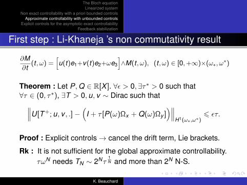
First step : Li-Khaneja ’s non commutativity result
∂M∂t
(t , ω) =[u(t)e1+v(t)e2+ωe3
]∧M(t , ω), (t , ω) ∈ [0,+∞)×(ω∗, ω
∗)
Theorem : Let P,Q ∈ R[X ]. ∀ε > 0,∃τ∗ > 0 such that∀τ ∈ (0, τ∗), ∃T > 0,u, v ∼ Dirac such that∥∥∥U[T+; u, v , .]−
(I + τ [P(ω)Ωx + Q(ω)Ωy ]
)∥∥∥H1(ω∗,ω∗)
6 ετ.
Proof : Explicit controls→ cancel the drift term, Lie brackets.
Rk : It is not sufficient for the global approximate controllability.τωN needs TN ∼ 2Nτ
1N and more than 2N N-S.
K. Beauchard
The Bloch equationLinearized system
Non exact controllability with a priori bounded controlsApproximate controllability with unbounded controls
Explicit controls for the asymptotic exact controllabilityFeedback stabilization
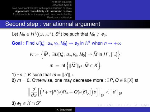
Second step : variationnal argument
Let M0 ∈ H1((ω∗, ω∗),S2) be such that M0 6= e3.
Goal : Find U[t+n ; un, vn,M0] e3 in H1 when n→ +∞
K :=
M ; ∃U[t+n ; un, vn,M0] M in H1, [...]
m := inf‖M ′‖L2 ; M ∈ K
1) ∃e ∈ K such that m = ‖e′‖L2
2) m = 0. Otherwise, one may decrease more : ∃P,Q ∈ R[X ] st∥∥∥ ddω
[(I + τ [P(ω)Ωx + Q(ω)Ωy ]
)e]∥∥∥
L2< ‖e′‖L2
3) e3 ∈ K ∩ S2
K. Beauchard
The Bloch equationLinearized system
Non exact controllability with a priori bounded controlsApproximate controllability with unbounded controls
Explicit controls for the asymptotic exact controllabilityFeedback stabilization
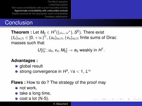
Conclusion
Theorem : Let M0 ∈ H1((ω∗, ω∗),S2). There exist
(tn)n∈N ∈ [0,+∞)N, (un)n∈N, (vn)n∈N finite sums of Diracmasses such that
U[t+n ; un, vn,M0]→ e3 weakly in H1.
Advantages :global resultstrong convergence in Hs, ∀s < 1, L∞
Flaws : How to do ? The strategy of the proof maynot work,take a long time,cost a lot (N-S).
K. Beauchard
The Bloch equationLinearized system
Non exact controllability with a priori bounded controlsApproximate controllability with unbounded controls
Explicit controls for the asymptotic exact controllabilityFeedback stabilization
4th part
Nonlinear system :explicit controls for the
asymptotic exactcontrollability
K. Beauchard
The Bloch equationLinearized system
Non exact controllability with a priori bounded controlsApproximate controllability with unbounded controls
Explicit controls for the asymptotic exact controllabilityFeedback stabilization
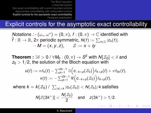
Explicit controls for the asymptotic exact controllability
Notations : - (ω∗, ω∗) = (0, π), f : (0, π)→ C identified with
f : R→ R, 2π periodic symmetric, N(f ) :=∑
n∈Z |cn(f )|.- M = (x , y , z), Z := x + iy
Theorem : ∃δ > 0 / ∀M0 : (0, π)→ S2 with N[Z0] < δ andz0 > 1/2, the solution of the Bloch equation with
u(t) := πδk (t)−∑2k−1
p=1 =(
c−k+p(Z0))δk+p(t) + πδ3k (t),
v(t) := −∑2k−1
p=1 <(
c−k+p(Z0))δk+p(t),
where k = k(Z0) /∑|n|>k |cn(Z0)| < N(Z0)/4 satisfies
N[Z(3k+)] <N(Z0)
2and z(3k+) > 1/2.
K. Beauchard
The Bloch equationLinearized system
Non exact controllability with a priori bounded controlsApproximate controllability with unbounded controls
Explicit controls for the asymptotic exact controllabilityFeedback stabilization
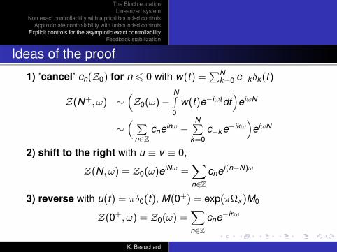
Ideas of the proof
1) ’cancel’ cn(Z0) for n 6 0 with w(t) =∑N
k=0 c−kδk (t)
Z(N+, ω) ∼(Z0(ω)−
N∫0
w(t)e−iωtdt)
eiωN
∼( ∑
n∈Zcneinω −
N∑k=0
c−ke−ikω)
eiωN
2) shift to the right with u ≡ v ≡ 0,
Z(N, ω) = Z0(ω)eiNω =∑n∈Z
cnei(n+N)ω
3) reverse with u(t) = πδ0(t), M(0+) = exp(πΩx )M0
Z(0+, ω) = Z0(ω) =∑n∈Z
cne−inω
K. Beauchard
The Bloch equationLinearized system
Non exact controllability with a priori bounded controlsApproximate controllability with unbounded controls
Explicit controls for the asymptotic exact controllabilityFeedback stabilization
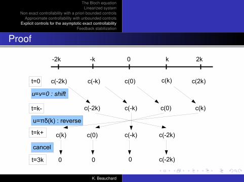
Proof
0-k-2k k 2k
t=0 c(-2k) c(-k) c(0) c(k) c(2k)
u=v=0 : shift
t=k- c(-2k) c(-k) c(0) c(k)
u=πδ(k) : reverse
t=k+ c(k) c(0) c(-k) c(-2k)
cancel
t=3k 0 0 0 c(-2k)
K. Beauchard
The Bloch equationLinearized system
Non exact controllability with a priori bounded controlsApproximate controllability with unbounded controls
Explicit controls for the asymptotic exact controllabilityFeedback stabilization
5th part
Nonlinear system :feedback stabilization
K. Beauchard
The Bloch equationLinearized system
Non exact controllability with a priori bounded controlsApproximate controllability with unbounded controls
Explicit controls for the asymptotic exact controllabilityFeedback stabilization
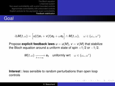
Goal
∂tM(t , ω) =[u(t)e1 + v(t)e2 + ωe3
]∧M(t , ω), ω ∈ (ω∗, ω
∗)
Propose explicit feedback laws u = u(M), v = v(M) that stabilizethe Bloch equation around a uniform state of spin +1/2 or −1/2.
M(t , ω) −−−−→t→+∞
e3 uniformly wrt ω ∈ (ω∗, ω∗)
Interest : less sensible to random perturbations than open loopcontrols
K. Beauchard
The Bloch equationLinearized system
Non exact controllability with a priori bounded controlsApproximate controllability with unbounded controls
Explicit controls for the asymptotic exact controllabilityFeedback stabilization
Strategy
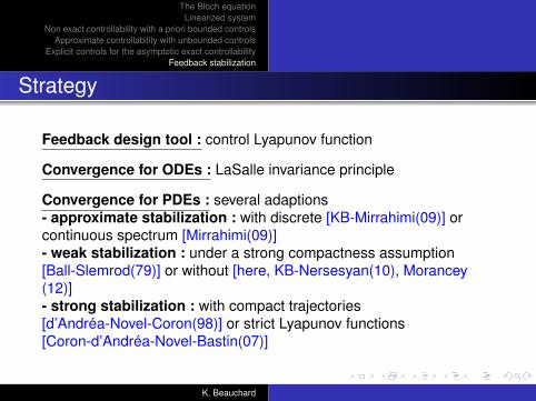
Feedback design tool : control Lyapunov function
Convergence for ODEs : LaSalle invariance principle
Convergence for PDEs : several adaptions- approximate stabilization : with discrete [KB-Mirrahimi(09)] orcontinuous spectrum [Mirrahimi(09)]- weak stabilization : under a strong compactness assumption[Ball-Slemrod(79)] or without [here, KB-Nersesyan(10), Morancey(12)]- strong stabilization : with compact trajectories[d’Andréa-Novel-Coron(98)] or strict Lyapunov functions[Coron-d’Andréa-Novel-Bastin(07)]
K. Beauchard
The Bloch equationLinearized system
Non exact controllability with a priori bounded controlsApproximate controllability with unbounded controls
Explicit controls for the asymptotic exact controllabilityFeedback stabilization
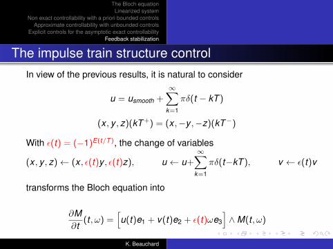
The impulse train structure controlIn view of the previous results, it is natural to consider
u = usmooth +∞∑
k=1
πδ(t − kT )
(x , y , z)(kT+) = (x ,−y ,−z)(kT−)
With ε(t) = (−1)E(t/T ), the change of variables
(x , y , z)← (x , ε(t)y , ε(t)z), u ← u+∞∑
k=1
πδ(t−kT ), v ← ε(t)v
transforms the Bloch equation into
∂M∂t
(t , ω) =[u(t)e1 + v(t)e2 + ε(t)ωe3
]∧M(t , ω)
K. Beauchard
The Bloch equationLinearized system
Non exact controllability with a priori bounded controlsApproximate controllability with unbounded controls
Explicit controls for the asymptotic exact controllabilityFeedback stabilization
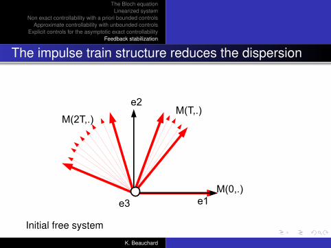
The impulse train structure reduces the dispersion
e1M(0,.)
M(T,.)M(2T,.)
e2
e3
Initial free system
∂M∂t
(t , ω) = ωe3 ∧M(t , ω), M(0, ω) = e1K. Beauchard
The Bloch equationLinearized system
Non exact controllability with a priori bounded controlsApproximate controllability with unbounded controls
Explicit controls for the asymptotic exact controllabilityFeedback stabilization
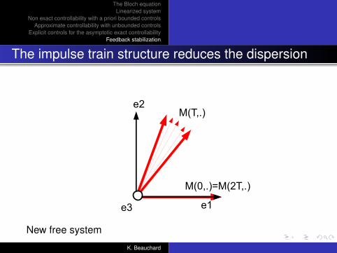
The impulse train structure reduces the dispersion
e1
M(T,.)e2
e3
M(0,.)=M(2T,.)
New free system
∂M∂t
(t , ω) = ε(t)ωe3 ∧M(t , ω), M(0, ω) = e1K. Beauchard
The Bloch equationLinearized system
Non exact controllability with a priori bounded controlsApproximate controllability with unbounded controls
Explicit controls for the asymptotic exact controllabilityFeedback stabilization
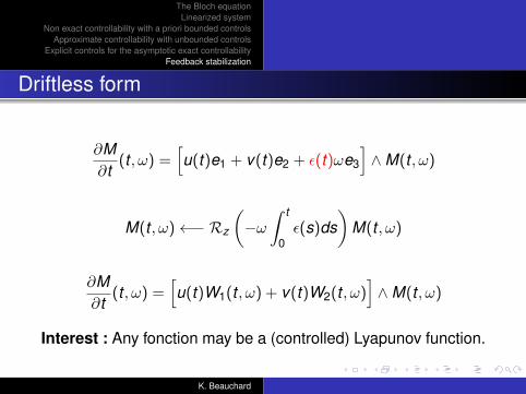
Driftless form
∂M∂t
(t , ω) =[u(t)e1 + v(t)e2 + ε(t)ωe3
]∧M(t , ω)
M(t , ω)←− Rz
(−ω
∫ t
0ε(s)ds
)M(t , ω)
∂M∂t
(t , ω) =[u(t)W1(t , ω) + v(t)W2(t , ω)
]∧M(t , ω)
Interest : Any fonction may be a (controlled) Lyapunov function.
K. Beauchard
The Bloch equationLinearized system
Non exact controllability with a priori bounded controlsApproximate controllability with unbounded controls
Explicit controls for the asymptotic exact controllabilityFeedback stabilization
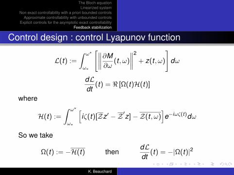
Control design : control Lyapunov function
L(t) :=
∫ ω∗
ω∗
[∥∥∥∥∂M∂ω
(t , ω)
∥∥∥∥2
+ z(t , ω)
]dω
dLdt
(t) = < [Ω(t)H(t)]
where
H(t) :=
∫ ω∗
ω∗
[iζ(t)[Zz ′ −Z ′z]−Z(t , ω)
]e−iωζ(t)dω
So we take
Ω(t) := −H(t) thendLdt
(t) = −|Ω(t)|2
K. Beauchard
The Bloch equationLinearized system
Non exact controllability with a priori bounded controlsApproximate controllability with unbounded controls
Explicit controls for the asymptotic exact controllabilityFeedback stabilization
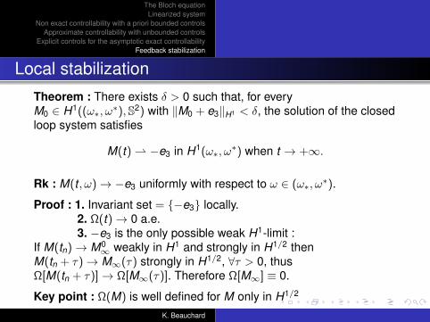
Local stabilizationTheorem : There exists δ > 0 such that, for everyM0 ∈ H1((ω∗, ω
∗),S2) with ‖M0 + e3‖H1 < δ, the solution of the closedloop system satisfies
M(t) −e3 in H1(ω∗, ω∗) when t → +∞.
Rk : M(t , ω)→ −e3 uniformly with respect to ω ∈ (ω∗, ω∗).
Proof : 1. Invariant set = −e3 locally.2. Ω(t)→ 0 a.e.3. −e3 is the only possible weak H1-limit :
If M(tn)→ M0∞ weakly in H1 and strongly in H1/2 then
M(tn + τ)→ M∞(τ) strongly in H1/2, ∀τ > 0, thusΩ[M(tn + τ)]→ Ω[M∞(τ)]. Therefore Ω[M∞] ≡ 0.
Key point : Ω(M) is well defined for M only in H1/2
K. Beauchard
The Bloch equationLinearized system
Non exact controllability with a priori bounded controlsApproximate controllability with unbounded controls
Explicit controls for the asymptotic exact controllabilityFeedback stabilization
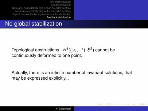
No global stabilization
Topological obstructions : H1((ω∗, ω∗),S2) cannot be
continuously deformed to one point.
Actually, there is an infinite number of invariant solutions, thatmay be expressed explicitly...
K. Beauchard
The Bloch equationLinearized system
Non exact controllability with a priori bounded controlsApproximate controllability with unbounded controls
Explicit controls for the asymptotic exact controllabilityFeedback stabilization
Numerical simulations
Parameters : (ω∗, ω∗) = (0,1), T = 2π, G := 1/(2T 2) x0(ω)
y0(ω)z0(ω)
:=
cos(π, ω)√
1− z0(ω)2
sin(π, ω)√
1− z0(ω)2
0.8− 0.1 sin(4πω)
.
Simulation until Tf = 50T
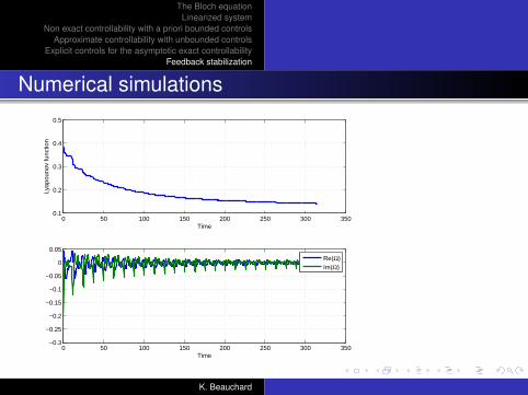
Conclusion : The convergence speed is rapid at the beginningbut decreases at the end.
K. Beauchard
The Bloch equationLinearized system
Non exact controllability with a priori bounded controlsApproximate controllability with unbounded controls
Explicit controls for the asymptotic exact controllabilityFeedback stabilization
Numerical simulations
0 50 100 150 200 250 300 3500.1
0.2
0.3
0.4
0.5
Time
Lyap
ouno
v fu
nctio
n
0 50 100 150 200 250 300 350−0.3
−0.25
−0.2
−0.15
−0.1
−0.05
0
0.05
Time
Re(Ω)Im(Ω)
K. Beauchard
The Bloch equationLinearized system
Non exact controllability with a priori bounded controlsApproximate controllability with unbounded controls
Explicit controls for the asymptotic exact controllabilityFeedback stabilization
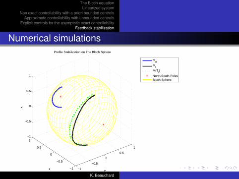
Adaptation to stabilize a variable profile
Target : Mf (ω)
Find R(ω) ∈ SO3 such that R(ω)Mf (ω) = −e3.Force N(t , ω) := R(ω)M(t , ω)→ −e3 when t → +∞(same strategy).
Proof OK forMf ∈ H1((ω∗, ω
∗), S2) with 〈Mf (ω),e3〉 6= 0, ∀ω ∈ (ω∗, ω∗),
‖M0 −Mf‖H1 small enough.
K. Beauchard
The Bloch equationLinearized system
Non exact controllability with a priori bounded controlsApproximate controllability with unbounded controls
Explicit controls for the asymptotic exact controllabilityFeedback stabilization
Numerical simulations
Parameters : ω∗ = 0, ω∗ = 1, T = 2π x0(ω)y0(ω)z0(ω)
:=
−0.35 sin(0.9πω − π/2)−0.35 cos(πω − π/2)√
1− x0(ω)2 − y0(ω)2
xf (ω)
yf (ω)zf (ω)
:=
−0.79 sin(πω − π/2)−0.79 cos(0.9πω − π/2)
−√
1− xf (ω)2 − yf (ω)2
Simulation until Tf = 80T
K. Beauchard
The Bloch equationLinearized system
Non exact controllability with a priori bounded controlsApproximate controllability with unbounded controls
Explicit controls for the asymptotic exact controllabilityFeedback stabilization
Numerical simulations
−1
−0.5
0
0.5
1
−1
−0.5
0
0.5
1−1
−0.5
0
0.5
1
y
Profile Stabilization on The Bloch Sphere
z
x
M0
Mf
M(Tf)
North/South PolesBloch Sphere
K. Beauchard
The Bloch equationLinearized system
Non exact controllability with a priori bounded controlsApproximate controllability with unbounded controls
Explicit controls for the asymptotic exact controllabilityFeedback stabilization
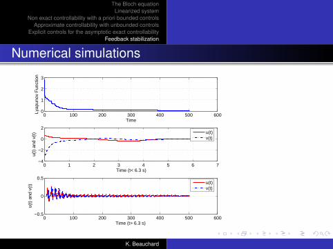
Numerical simulations
0 100 200 300 400 500 6000
1
2
3
Time
Lyap
unov
Fun
ctio
n
0 1 2 3 4 5 6 7−4
−2
0
2
Time (t< 6.3 s)
u(t)
and
v(t
) u(t)v(t)
0 100 200 300 400 500 600−0.5
0
0.5
Time (t> 6.3 s)
u(t)
and
v(t
) u(t)v(t)
K. Beauchard
The Bloch equationLinearized system
Non exact controllability with a priori bounded controlsApproximate controllability with unbounded controls
Explicit controls for the asymptotic exact controllabilityFeedback stabilization
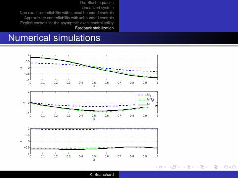
Numerical simulations
0 0.1 0.2 0.3 0.4 0.5 0.6 0.7 0.8 0.9 1−1
−0.5
0
0.5
1
ω
x
0 0.1 0.2 0.3 0.4 0.5 0.6 0.7 0.8 0.9 1−1
0
1
ω
y
M0
M(Tf)
Mf
0 0.1 0.2 0.3 0.4 0.5 0.6 0.7 0.8 0.9 1−1
−0.5
0
0.5
1
ω
z
K. Beauchard
The Bloch equationLinearized system
Non exact controllability with a priori bounded controlsApproximate controllability with unbounded controls
Explicit controls for the asymptotic exact controllabilityFeedback stabilization
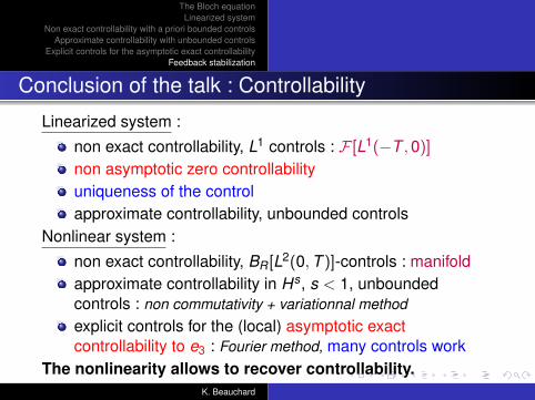
Conclusion of the talk : Controllability
Linearized system :
non exact controllability, L1 controls : F [L1(−T ,0)]
non asymptotic zero controllabilityuniqueness of the controlapproximate controllability, unbounded controls
Nonlinear system :
non exact controllability, BR[L2(0,T )]-controls : manifoldapproximate controllability in Hs, s < 1, unboundedcontrols : non commutativity + variationnal methodexplicit controls for the (local) asymptotic exactcontrollability to e3 : Fourier method, many controls work
The nonlinearity allows to recover controllability.K. Beauchard
The Bloch equationLinearized system
Non exact controllability with a priori bounded controlsApproximate controllability with unbounded controls
Explicit controls for the asymptotic exact controllabilityFeedback stabilization
Conclusion of the talk : Stabilization
impulse train controldriftless formcontrol Lyapunov function : H1-distance to the targetexplicit damping feedback lawsweak H1 local stabilization
K. Beauchard
The Bloch equationLinearized system
Non exact controllability with a priori bounded controlsApproximate controllability with unbounded controls
Explicit controls for the asymptotic exact controllabilityFeedback stabilization
Open problems, perspectives
exact controllability in finite time with unboundedcontrols ?strong stabilization with the same feedback laws ?explicit feedbacks for the semi-global stabilizationconvergence rates ? arbitrarily fast stabilization ?
K. Beauchard
The Bloch equationLinearized system
Non exact controllability with a priori bounded controlsApproximate controllability with unbounded controls
Explicit controls for the asymptotic exact controllabilityFeedback stabilization
References
1 K. Beauchard, J.-M. Coron and P. Rouchon. Controllabilityissues for continuous-spectrum systems and ensemblecontrollability of Bloch equations. CMP, 296, 2, June 2010,p.525-557.
2 K. Beauchard, P. Pereira da Silva and P. Rouchon. Stabilizationand motion planning for an ensemble of half spin systems.Automatica 48, pp.68-76, 2012.
3 K. Beauchard, P. Pereira da Silva and P. Rouchon. Stabilizationof an arbitrary profile for an ensemble of half-spin systems.Automatica (to appear).
K. Beauchard