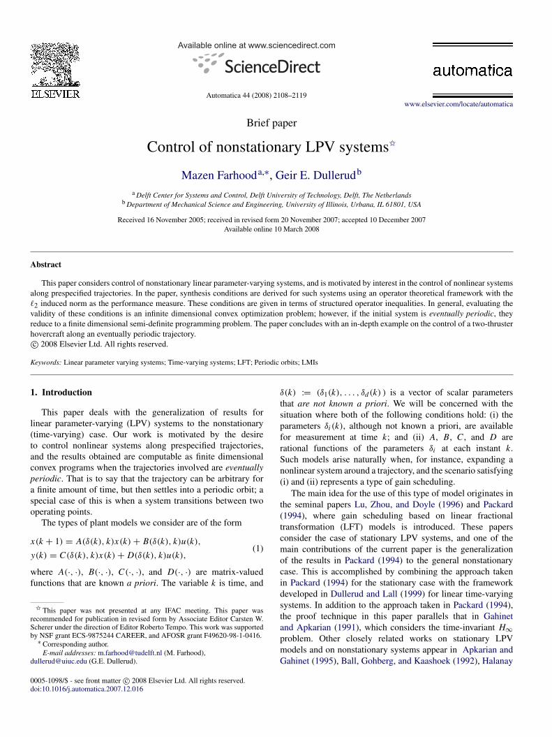
Automatica 44 (2008) 2108–2119www.elsevier.com/locate/automatica

Brief paper

Control of nonstationary LPV systemsI

Mazen Farhooda,∗, Geir E. Dullerudb

a Delft Center for Systems and Control, Delft University of Technology, Delft, The Netherlandsb Department of Mechanical Science and Engineering, University of Illinois, Urbana, IL 61801, USA

Received 16 November 2005; received in revised form 20 November 2007; accepted 10 December 2007Available online 10 March 2008

Abstract

This paper considers control of nonstationary linear parameter-varying systems, and is motivated by interest in the control of nonlinear systemsalong prespecified trajectories. In the paper, synthesis conditions are derived for such systems using an operator theoretical framework with the`2 induced norm as the performance measure. These conditions are given in terms of structured operator inequalities. In general, evaluating thevalidity of these conditions is an infinite dimensional convex optimization problem; however, if the initial system is eventually periodic, theyreduce to a finite dimensional semi-definite programming problem. The paper concludes with an in-depth example on the control of a two-thrusterhovercraft along an eventually periodic trajectory.c© 2008 Elsevier Ltd. All rights reserved.

Keywords: Linear parameter varying systems; Time-varying systems; LFT; Periodic orbits; LMIs

1. Introduction

This paper deals with the generalization of results forlinear parameter-varying (LPV) systems to the nonstationary(time-varying) case. Our work is motivated by the desireto control nonlinear systems along prespecified trajectories,and the results obtained are computable as finite dimensionalconvex programs when the trajectories involved are eventuallyperiodic. That is to say that the trajectory can be arbitrary fora finite amount of time, but then settles into a periodic orbit; aspecial case of this is when a system transitions between twooperating points.

The types of plant models we consider are of the form

x(k + 1) = A(δ(k), k)x(k)+ B(δ(k), k)u(k),

y(k) = C(δ(k), k)x(k)+ D(δ(k), k)u(k),(1)

where A(·, ·), B(·, ·), C(·, ·), and D(·, ·) are matrix-valuedfunctions that are known a priori. The variable k is time, and

I This paper was not presented at any IFAC meeting. This paper wasrecommended for publication in revised form by Associate Editor Carsten W.Scherer under the direction of Editor Roberto Tempo. This work was supportedby NSF grant ECS-9875244 CAREER, and AFOSR grant F49620-98-1-0416.

∗ Corresponding author.E-mail addresses: m.farhood@tudelft.nl (M. Farhood),

dullerud@uiuc.edu (G.E. Dullerud).

0005-1098/$ - see front matter c© 2008 Elsevier Ltd. All rights reserved.doi:10.1016/j.automatica.2007.12.016

δ(k) := (δ1(k), . . . , δd(k) ) is a vector of scalar parametersthat are not known a priori. We will be concerned with thesituation where both of the following conditions hold: (i) theparameters δi (k), although not known a priori, are availablefor measurement at time k; and (ii) A, B, C , and D arerational functions of the parameters δi at each instant k.Such models arise naturally when, for instance, expanding anonlinear system around a trajectory, and the scenario satisfying(i) and (ii) represents a type of gain scheduling.

The main idea for the use of this type of model originates inthe seminal papers Lu, Zhou, and Doyle (1996) and Packard(1994), where gain scheduling based on linear fractionaltransformation (LFT) models is introduced. These papersconsider the case of stationary LPV systems, and one of themain contributions of the current paper is the generalizationof the results in Packard (1994) to the general nonstationarycase. This is accomplished by combining the approach takenin Packard (1994) for the stationary case with the frameworkdeveloped in Dullerud and Lall (1999) for linear time-varyingsystems. In addition to the approach taken in Packard (1994),the proof technique in this paper parallels that in Gahinetand Apkarian (1991), which considers the time-invariant H∞

problem. Other closely related works on stationary LPVmodels and on nonstationary systems appear in Apkarian andGahinet (1995), Ball, Gohberg, and Kaashoek (1992), Halanay

M. Farhood, G.E. Dullerud / Automatica 44 (2008) 2108–2119 2109

and Ionescu (1994), Helmersson (1995), Iglesias (1996), Lee(1997), Lu et al. (1996), Wu (2001) and Wu, Packard, andBecker (1996) respectively.

We remark that in many cases, when deriving anonstationary linear parameter-varying (NSLPV) model suchas (1) along a trajectory, it is possible to find a stationary LPVmodel that also parameterizes the nonlinear system along thetrajectory. The main advantages that a nonstationary model willtypically have are: (a) from an algebraic point of view, onecan easily construct situations in which the stationary LPVsystem is not stabilizable, but the nonstationary one is; and(b) the set of systems parameterized by the stationary modelwill typically be much larger than that by the correspondingnonstationary one, and thus may needlessly limit the closed-loop performance of the model. Indeed, the situation in (a) canbe viewed as an extreme version of type (b) conservatism. Intime-varying systems, it is well known that systems can bestabilizable even though the state space matrices, pointwise intime, are not stabilizable; this serves as an analogy for (a) in thecase of standard systems.

The main contributions of this paper are:

• The development of general synthesis conditions for controlof NSLPV systems; these conditions are infinite dimensionaland convex. As with the stationary case, the conditions weobtain are only sufficient for an LPV synthesis to exist, butare necessary and sufficient for the case where there are noparameters δi ; that is, the nominal system is a standard time-varying system. When the model in (1) is stationary, theconditions derived are exactly the ones in Packard (1994).

• The introduction of the concept of an eventually periodicLPV system, and results showing that, for these systems, thegeneral synthesis conditions obtained become linear matrixinequalities (LMIs), thus making them readily computable.Eventually periodic systems contain both finite horizonand periodic systems as special cases. In addition to theapplication already mentioned of trajectories that eventuallysettle into a periodic orbit, eventually periodic systemsnaturally arise when considering problems in which the planthas an uncertain initial state.

The paper is based on Farhood (2005) and is organized asfollows. In Section 2, we define our notation and introducesome useful machinery. We formulate the LPV problem ofinterest in Section 3, and develop analysis and synthesis resultsin Section 4. In Section 5, we consider eventually periodic LPVsystems, and we conclude in Section 6 with an example on thecontrol of a two-thruster hovercraft along an eventually periodicpath.

2. Preliminaries

The set of real n × m matrices is denoted by Rn×m . Thelinear space of elements x = (x(0), x(1), x(2), . . .), withx(k) ∈ Rn(k), is denoted by `(Rn). We define the Hilbertspace `2(Rn) as the subspace of `(Rn) consisting of elementsx ∈ `(Rn) such that ‖x‖

2=

∑∞

k=0 x(k)∗x(k) < ∞. Whenthe spatial dimensions n(k) are either evident or irrelevant to

the discussion, we will simply use the abbreviations `2 and `.We denote the space of bounded linear operators mapping `2to `2 by L(`2), and the `2 to `2 induced norm of an operatorX by ‖X‖. The adjoint of X is written X∗. When an operatorX ∈ L(`2) is self-adjoint, we use X ≺ 0 to mean it is negativedefinite; that is there exists a number α > 0 such that, for allnonzero x ∈ `2, the inequality 〈x, X x〉 < −α‖x‖

2 holds, where〈·, ·〉 denotes the inner product. Given a sequence of dimensionsn1(k), n2(k), . . . , n p(k), we define the Hilbert space direct sum

`(n1,...,n p)

2 := `2(Rn1)⊕ `2(Rn2)⊕ · · · ⊕ `2(Rn p ). Let 0i× j andI j denote an i × j zero matrix and a j × j identity matrixrespectively. Other notations used in this paper are

I n`2

:= diag(In(0), In(1), In(2), . . .),

I(n1,...,n p)

`2:= diag(I n1

`2, I n2`2, . . . , I

n p`2),

0n×m`2

:= diag(0n(0)×m(0), 0n(1)×m(1), . . .),

and

0(n1,...,n p)×(m1,...,mq )

`2:=

[01×n1`2

· · · 01×n p`2

]∗

×

[01×m1`2

· · · 01×mq`2

].

A key operator used in the paper is the unilateral shift Z , definedas follows:

Z : `2

(Rn(1),Rn(2), . . .

)→ `2

(Rn(0),Rn(1),Rn(2), . . .

)(a(1), a(2), . . .)

Z7−→ (0, a(1), a(2), . . .).

Clearly this definition is extendable to `, and in the sequel,we will not distinguish between these mappings.

Following the notation and approach in Dullerud and Lall(1999), we make the following definitions. First, we say a linearoperator Q mapping `(Rm(0),Rm(1), . . .) to `(Rn(0),Rn(1), . . .)

is block-diagonal if there exists a sequence of matricesQ(k) in Rn(k)×m(k) such that, for all w, z, if z = Qw,then z(k) = Q(k)w(k). Then Q has the representationdiag(Q(0), Q(1), Q(2), . . .).

Suppose F , G, R and S are block-diagonal operators, and let

A be a partitioned operator of the form A =

[F GR S

]. Then we

define

[[A]] := diag([

F(0) G(0)R(0) S(0)

],

[F(1) G(1)R(1) S(1)

], . . .

).

Clearly, [[A]] is simply A with the rows and columns permuted

appropriately so that [[A ]]k =

[F(k) G(k)R(k) S(k)

]. It is easy to see

that [[A + B]] = [[A]] + [[B]] and [[AC]] = [[A]][[C]] hold forappropriately dimensioned operators, and that A ≺ β I holds ifand only if [[A]] ≺ β I , where β is a scalar. Namely, the [[•]]

operation is a homomorphism from partitioned operators withblock-diagonal entries to block-diagonal operators.

3. Problem formulation

We will be concerned with a particular subclass of modelsof the form in (1), where the dependence of the state-space

2110 M. Farhood, G.E. Dullerud / Automatica 44 (2008) 2108–2119

matrices on the parameters δi is given in terms of a feedbackcoupling. These types of systems are commonly referredto as LFT systems, in which the state-space dependenceon the parameters is rational. Models of this subclass arethe straightforward generalization of the LPV systems firstintroduced in Lu et al. (1996) and Packard (1994).

3.1. NSLPV plant

Let Gδ be a discrete-time LFT system defined by thefollowing state-space equations:

x(k + 1)α(k)z(k)y(k)

=

Ass(k) Asp(k) B1s(k) B2s(k)Aps(k) App(k) B1p(k) B2p(k)C1s(k) C1p(k) D11(k) D12(k)C2s(k) C2p(k) D21(k) 0

×

x(k)β(k)w(k)u(k)

, (2)

β(k) = diag(δ1(k)In1(k), . . . , δd(k)Ind (k))α(k)= ∆(k)α(k),

x(0) = 0, for w ∈ `2. The signals w(k) and z(k) denote theexogenous disturbances and errors, respectively, whereas u(k)denotes the applied control and y(k) the measurements. Thevectors x(k), α(k), β(k), z(k),w(k), y(k), and u(k) are real andhave time-varying dimensions, denoted by n0(k), n(k), n(k),nz(k), nw(k), ny(k), and nu(k) respectively. The parametersδi (k) are real scalars such that |δi (k)| ≤ 1 for all k ≥ 0and i = 1, 2, . . . , d , and the associated dimensions ni (k)satisfy

∑di=1 ni (k) = n(k). We assume that I − App(k)∆(k)

is invertible for all k ≥ 0 so that this LFT system is well posed,and thus there are unique solutions in ` to (2). Also, we assumeall the state-space matrices are uniformly bounded functionsof time.

Using the previously defined notation, clearly the matrixsequences Ass(k), B1s(k), B2s(k), C1s(k), C2s(k), D11(k),D12(k), and D21(k) define bounded block-diagonal operators.The blocks of matrix ∆(k) naturally partition α(k) and β(k)into d separate vector-valued channels, conformably withwhich we partition the following state-space matrices:

Asp(k) =

[A1

sp(k) A2sp(k) · · · Ad

sp(k)]

C1p(k) =

[C1

1p(k) C21p(k) · · · Cd

1p(k)]

C2p(k) =

[C1

2p(k) C22p(k) · · · Cd

2p(k)]

App(k) =

A11pp(k) · · · A1d

pp(k)...

. . ....

Ad1pp(k) · · · Add

pp(k)

Aps(k) =

A1

ps(k)A2

ps(k)...

Adps(k)

(3)

B1p(k) =

B1

1p(k)B2

1p(k)...

Bd1p(k)

B2p(k) =

B1

2p(k)B2

2p(k)...

Bd2p(k)

,where Ai

sp(k) ∈ Rn0(k+1)×ni (k), Ai jpp(k) ∈ Rni (k)×n j (k),

Aips(k) ∈ Rni (k)×n0(k), Bi

1p(k) ∈ Rni (k)×nw(k), Bi2p(k) ∈

Rni (k)×nu(k), C i1p(k) ∈ Rnz(k)×ni (k), and C i

2p(k) ∈ Rny(k)×ni (k).The matrix sequence of each of the elements of the state-spacematrices in (3) defines a bounded block-diagonal operator; andso we construct from the sequence of each of these state-space matrices a partitioned operator, each of whose elementsis block diagonal and defined in the obvious way. For instance,the matrix sequences A1

sp(k), . . . , Adsp(k) define block-diagonal

operators that compose the partitioned operator Asp. With Zbeing the shift, we can rewrite our system equations as

xα

zy

=

Z Ass Z Asp Z B1s Z B2sAps App B1p B2pC1s C1p D11 D12C2s C2p D21 0

xβ

w

u

,[

xβ

]= diag(I n0

`2,∆1, . . . ,∆d)

[xα

]= ∆

[xα

],

(4)

where x ∈ `(Rn0), w ∈ `2(Rnw ), q ∈ `(Rnq ) for q = u, z, y,

β = (β1, . . . , βd), α = (α1, . . . , αd), βi , αi ∈ `(Rni ), and∆i = diag(δi (0)Ini (0), δi (1)Ini (1), δi (2)Ini (2), . . .).

We now introduce some convenient definitions andnotations. To start, we define

A :=

[Ass AspAps App

], B1 :=

[B1sB1p

], B2 :=

[B2sB2p

],

C1 :=[C1s C1p

], C2 :=

[C2s C2p

].

We also define Z = diag(Z , I ), which is partitioned similarlyto A. This partitioning is clearly conformable to that of ∆ =

diag(∆s,∆p), where ∆s = I`2 and ∆p = diag(∆1, . . . ,∆d).Notice that [[∆p ]]k = ∆(k). Moreover, we define 1 := {∆ ∈

L(`(n0,...,nd )2 ) : ∆ is partitioned as in (4), ‖∆‖ ≤ 1}. The set of

systems Gδ for all ∆ ∈ 1 defines an NSLPV model Gδ , namelyGδ = {Gδ : ∆ ∈ 1}.

We now define the basic notions of well-posedness andstability for NSLPV models.

Definition 1. An NSLPV model Gδ is

(i) well posed if I − ∆p App has an algebraic inverse (notnecessarily bounded) for all ∆ ∈ 1;

(ii) `2-stable if I − ∆Z A has a bounded inverse for all ∆ ∈ 1.

It follows from (ii) that, when a system is `2-stable, thereexists a unique (x, β) ∈ `

(n0,...,nd )2 satisfying (4). We refer the

reader to Farhood and Dullerud (2007) for an in-depth treatmentof well-posedness and stability for NSLPV systems.

The parameters δi are not uncertain, and while not known apriori, they are available for measurement at each k. Next weincorporate these plant parameters into the control design.

M. Farhood, G.E. Dullerud / Automatica 44 (2008) 2108–2119 2111

3.2. Controller and closed-loop system

Given an operator ∆ ∈ 1 and an associated system Gδ , wesuppose this system is being controlled by a controller Kδ thathas a similar structure as Gδ . The controller is defined by thestate-space equationsx K

αK

u

=

Z AKss Z AK

sp Z BKs

AKps AK

pp BKp

C Ks C K

p DK

x K

βK

y

,[

x K

βK

]= diag(I r0

`2,∆K

1 , . . . ,∆Kd )

[x K

αK

]= ∆K

[x K

αK

],

(5)

where x K∈ `(Rm0), βK

= (βK1 , . . . , β

Kd ), α

K=

(αK1 , . . . , α

Kd ), β

Ki , αK

i ∈ `(Rmi ), and the block-diagonaloperator ∆K

i = diag(δi (0)Imi (0), δi (1)Imi (1), . . .). We willderive the proper values for the controller dimensions in thenext section. Note that the parameters δ that affect the controllerare the same as those that affect the plant. The well-posednessof this LFT can always be guaranteed by slightly perturbing∆K , if necessary, to ensure that I − AK

pp∆K is invertible.

We write the realization of the closed-loop system as

xcl = ∆cl Z2 Acl xcl + ∆cl Z2 Bclw, z = Ccl xcl + Dclw,

where xcl is the column vector (x, β, x K , βK ), ∆cl =

diag(∆,∆K ), Z2 = diag(Z , Z), and the remaining operatorsare defined in the obvious way. We denote this realization bySδ , and hence the closed-loop NSLPV system Sδ is given bySδ = {Sδ : ∆ ∈ 1}. Note that, for NSLPV systems, thestandard form of ∆ is the one given in (4) and (5). It is obviousthat ∆cl is not of the standard form, but this can be remediedeasily by a change of basis via a permutation. Specifically, thereexists a unique permutation P such that

P∗∆cl P = ∆L= diag(I s0

`2,∆L

1 , . . . ,∆Ld ), (6)

where si = ni + mi , ∆Li = diag(δi (0)Isi (0), δi (1)Isi (1), . . .);

clearly, ∆L conforms with the standard form. Then, for all∆ ∈ 1, an equivalent realization for Sδ is given by[

x L

αL

]z

=

[Z AL Z BL

C L DL

] [x L

βL

]w

,[

x L

βL

]= ∆L

[x L

αL

],

where x L∈ `(Rs0), αL

= (αL1 , . . . , α

Ld ), β

L= (βL

1 , . . . , βLd ),

αLi , β

Li ∈ `(Rsi ), and AL

= (Z∗ P∗ Z2)Acl P ,

BL= (Z∗ P∗ Z2)Bcl , C L

= Ccl P, DL= Dcl . (7)

Notice that Z AL= Z Z∗(P∗ Z2 Acl P) = P∗ Z2 Acl P and

Z BL= P∗ Z2 Bcl . For convenience, we define 1L

:= {∆L∈

L(`(s0,...,sd )2 ) : ∆L is partitioned as in (6),

∥∥∆L∥∥ ≤ 1}.

We will denote the NSLPV controller by Kδ , instead of Kδ ,to emphasize that the controller parameters are not arbitrary butrather they are the same as those of the plant.

4. Synthesis

The following definition expresses our synthesis goal.

Definition 2. A controller Kδ is an admissible synthesis for anNSLPV plant Gδ if the closed-loop NSLPV system Sδ is `2-stable and the input-output mapping w 7→ z satisfies

‖w 7→ z‖ =

∥∥∥C L(I − ∆L Z AL)−1∆L Z BL+ DL

∥∥∥ < 1

for all ∆L∈ 1L .

Lemma 3. The closed-loop NSLPV system Sδ is `2-stable andthe performance inequality ‖w 7→ z‖ < 1 is satisfied for all∆ ∈ 1 if there exists a positive definite operator X L in thecommutant of 1L such that[

Z AL Z BL

C L DL

]∗ [X L 00 I

] [Z AL Z BL

C L DL

]−

[X L 00 I

]≺ 0. (8)

This is a generalization of the sufficiency part of the Kalman-Yakubovich-Popov Lemma. Its proof is routine and so isomitted. Note that inequality (8) is necessary and sufficient inthe purely time-varying case (Yacubovich, 1975); but, in ourcase, it is in general only sufficient, and thus this may introduceconservatism into our approach.

At this point, we define the set X L to consist of positivedefinite operators X L of the form

X L= diag(X L

0 , X L1 , . . . , X L

d ) � 0,

where each X Li is block diagonal, namely

X Li = diag(X L

i (0), X Li (1), . . .), with X L

i (k) ∈ Rsi (k)×si (k).

Proposition 4. A positive definite solution X L , belonging tothe commutant of 1L , exists to inequality (8) if and only if asolution X L

∈ X L exists.

Proof. The proof of the “if” direction is immediate since X L isclearly a subset of the commutant of 1L .

We now prove the “only if” direction. Suppose X L is apositive definite operator in the commutant of 1L satisfying (8).Then X L has the form X L

= diag(X L0 , X L

1 , . . . , X Ld ) �

0, where, for i = 1, 2, . . . , d, each operator X Li is block

diagonal with [[X Li ]]k = X L

i (k) ∈ Rsi (k)×si (k), whereas X L0 ∈

L(`2(Rs0)) and is not necessarily block diagonal. Followinga very similar argument to that used in the proof of Dullerudand Lall (1999, Theorem 11), we can construct from X L anoperator X L

= diag(X L0 , X L

1 , . . . , X Ld ) ∈ X L that also solves

(8) such that X L0 is a block-diagonal operator whose elements

are the blocks on the diagonal of X L0 and X L

i = X Li for

i = 1, . . . , d. �

The procedure henceforth is very similar to the ones givenin Dullerud and Lall (1999) and Gahinet and Apkarian (1991)for LTI and LTV systems respectively, and so we present it

2112 M. Farhood, G.E. Dullerud / Automatica 44 (2008) 2108–2119

very briefly. Before proceeding, it is convenient to define thenotations n = (n0, . . . , nd) and m = (m0, . . . ,md). Now,consider the following closed-loop parametrization:

Acl = A + B JC, Bcl = B + B J D21,

Ccl = C + D12 JC, Dcl = D11 + D12 J D21,(9)

where operator J describes the controller realization, namely

J :=

AKss AK

sp BKs

AKps AK

pp BKp

C Ks C K

p DK

,and the other operators are defined as follows:

C :=

[C1 0nz×m

`2

], D12 :=

[0nz×m`2

D12

],

A :=

[A 00 0m×m

`2

], B :=

[B1

0m×nw`2

],

B :=

[0 B2

I m`2

0

],

C :=

[0 I m

`2C2 0

], D21 :=

[0m×nw`2D21

].

Lemma 5. The controller Kδ described by the operator J is anadmissible synthesis if there exists X L

∈ X L such that

HX LP

+ Q∗ J ∗ R + R∗ J Q ≺ 0, (10)

where R =

[B∗ 0(m,nu)×(n,m)

`20(m,nu)×nw`2

D∗

12

],

Q =

[0(m,ny)×(n,m)`2

C D21 0(m,ny)×nz`2

],

HX LP

=

−Z∗

2(XLP )

−1 Z2 A B 0A∗

−X LP 0 C∗

B∗ 0 −I D∗

110 C D11 −I

,X L

P = P X L P∗,

and the permutation P is as defined in (6).

Proof. The controller is admissible if there exists a solutionX L

∈ X L to inequality (8). Pre- and post-multiplying (8) bydiag(P, I ) and diag(P∗, I ) respectively and then substitutingthe definitions from (7), we get the equivalent inequality[

Acl BclCcl Dcl

]∗ [Z∗

2 P X L P∗ Z2 00 I

] [Acl BclCcl Dcl

]−

[P X L P∗ 0

0 I

]≺ 0.

Applying the Schur complement formula twice and thensubstituting expressions (9) give the desired result. �

Lemma 6. There exists a partitioned operator J satisfyinginequality (10) if and only if

W ∗

R HX LP

WR ≺ 0 and W ∗

Q HX LP

WQ ≺ 0, (11)

where Im WR = Ker R, Im WQ = Ker Q, W ∗

R WR = I , andW ∗

Q WQ = I .

This lemma is a generalization of a similar result in Gahinetand Apkarian (1991). Its proof is nearly identical to the onepresented in Dullerud and Lall (1999) and so we omit it.

One problem with the preceding result is that inequalities(11) are not affine in X L

P , since both X LP and (X L

P )−1 appear in

HX LP

. To remedy this, given X L= diag(X L

0 , . . . , X Ld ) ∈ X L ,

we conveniently partition the matrix blocks as

X Li (k) =

[X i (k) Xb

i (k)Xb

i (k)∗ X c

i (k)

],

where the matrices X i (k) ∈ Rni (k)×ni (k), Xbi (k) ∈ Rni (k)×mi (k)

and X ci (k) ∈ Rmi (k)×mi (k). Note that the sequences X i (k),

Xbi (k), and X c

i (k) define block-diagonal operators X i , Xbi and

X ci respectively. With X L

P = P X L P∗, it is straightforward toverify that

X LP =

[X Xb

(Xb)∗ X c

],

where X = diag(X0, . . . , Xd), and Xb and X c are definedsimilarly. Clearly, since (X L

P )−1

= P(X L)−1 P∗, then (X LP )

−1

has the same form as X LP , namely

X LP =

[X Xb

(Xb)∗ X c

], (X L

P )−1

=

[Y Y b

(Y b)∗ Y c

]. (12)

We define the set X to consist of positive definite operatorsX = diag(X0, . . . , Xd), where each X i ∈ L(`ni

2 ) is blockdiagonal. Then, X and Y from (12) are elements of X .

Lemma 7. Suppose X, Y ∈ X and mi is a positive integer forall i = 0, 1, . . . , d. Then there exists an operator X L

P � 0satisfying (12) if and only if, for all k ≥ 0, i = 0, 1, . . . , d,[

Y II X

]� 0 and rank

[Yi (k) I

I X i (k)

]≤ ni (k)+ mi (k).

The proof of this is nearly identical to its matrix versionfound in Packard (1994) and so we do not include it here.

The next theorem transforms (11) into convex conditions.

Theorem 8. There exists an admissible synthesis Kδ forNSLPV plant Gδ , with dimensions mi ≤ ni for all i =

0, 1, . . . , d, if there exist operators X, Y ∈ X such that

N∗

Y

{F

[Y

I

]F∗

−

[Z∗Y Z

I

]}NY ≺ 0,

N∗

X

{F∗

[Z∗ X Z

I

]F −

[X

I

]}NX ≺ 0,[

Y II X

]� 0, with F =

[A B1

C1 D11

],

(13)

where the operators NY , NX satisfy

Im NY = Ker[B∗

2 D∗

12

], N∗

Y NY = I,

Im NX = Ker[C2 D21

], N∗

X NX = I.

M. Farhood, G.E. Dullerud / Automatica 44 (2008) 2108–2119 2113

Proof. Suppose there exist operators X and Y satisfying theconditions in (13). Then by invoking Lemma 7, for somepositive integers mi ≤ ni , there exists an operator X L

P thatsatisfies (12). Set N∗

Y =[V ∗

1 V ∗

2

], where V2 is block diagonal

with V2(k) ∈ Rnz(k)×?, and V1 is a partitioned operator,each of whose elements is block diagonal, namely V1 =[V 0

1∗

V 11

∗· · · V d

1∗]∗

with V i1 (k) ∈ Rni (k)×?. Then, the

first condition in the theorem statement is equivalent to[H V ∗

1 B1 + V ∗

2 D11B∗

1 V1 + D∗

11V2 −I

]≺ 0,

where H = V ∗

1 (AY A∗− Z∗Y Z)V1 + V ∗

1 AY C∗

1 V2 +

V ∗

2 C1Y A∗V1 + V ∗

2 (C1Y C∗

1 − I )V2. Applying the Schurcomplement formula to this condition, we equivalently get

−V ∗

1 Z∗Y Z V1 − V ∗

2 V2 +[V ∗

1 A + V ∗

2 C1 0 V ∗

1 B1 + V ∗

2 D11]

×

Y Y b 0(Y b)∗ Y c 0

0 0 I

A∗V1 + C∗

1 V20

B∗

1 V1 + D∗

11V2

≺ 0.

In order to invert (X LP )

−1=

[Y Y b

(Y b)∗ Y c

], we apply the Schur

complement formula again and so the last inequality holds ifand only if the following operator

−V ∗

1 Z∗Y Z V1 − V ∗

2 V2 V ∗

1 A + V ∗

2 C1 0 V ∗

1 B1 + V ∗

2 D11

A∗V1 + C∗

1 V2 −X −Xb 00 −(Xb)∗ −X c 0

B∗

1 V1 + D∗

11V2 0 0 −I

is negative definite. Setting WR =

[V ∗

1 0 0 V ∗2

0 0 I (n,m,nw)`2

0

]∗

, it is not

difficult to see that the preceding negative definite operator isexactly W ∗

R HX LP

WR . Observe that, given R from (10), Im WR =

Ker R and W ∗

R WR = I . A similar argument starting withthe second condition in the theorem statement shows that thecondition W ∗

Q HX LP

WQ ≺ 0 from (11) holds. Thus, we have

shown that conditions (13) hold if and only if there exists an X LP

satisfying (12) such that W ∗

R HX LP

WR ≺ 0 and W ∗

Q HX LP

WQ ≺

0. Therefore, by Lemma 6, there exists an admissible synthesisfor Gδ . �

Note that if we partition Y and X as: Y = diag(Ys, Yp) andX = diag(Xs, X p), where Ys = Y0, Yp = diag(Y1, . . . , Yd),with Xs and X p defined similarly, and if we define

Im [[NY ]]k = Ker[[[B∗

2 ]]k D∗

12(k)],

Im [[NX ]]k = Ker[[[C2 ]]k D21(k)

],

which are directly related to NY and NX , then the conditions ofTheorem 8 are clearly equivalent to the existence of β > 0 suchthat, for all k ≥ 0, we have

(S1) [[NY ]]∗

k

{[[F ]]k diag

(Ys(k), [[Yp ]]k, I

)[[F ]]

∗

k

−diag(Ys(k + 1), [[Yp ]]k, I

)}[[NY ]]k ≺ −β I,

(S2) [[NX ]]∗

k

{[[F ]]

∗

k diag(Xs(k + 1), [[X p ]]k, I

)[[F ]]k

−diag(Xs(k), [[X p ]]k, I

)}[[NX ]]k ≺ −β I,

(S3)[[[Y ]]k I

I [[X ]]k

]� 0, where F =

[A B1

C1 D11

].

This gives a recursive matrix form of the solution.We now briefly outline the procedure for constructing a

controller from the solutions X and Y . To start, define mi (k) :=

rank ([[X i ]]k −[[Yi ]]k) ≤ ni (k) for i = 0, 1, . . . , d. UsingLemma 7, construct an operator X L

P satisfying (12). Then,solve inequality (10) for the controller realization J . Allof the preceding steps are convex but infinite-dimensionalcomputations. See Gahinet and Apkarian (1991) or Packard(1994) for more details on this procedure.

5. Eventually periodic systems

We start by defining an eventually periodic operator.

Definition 9. A block-diagonal mapping P on `2 is (h, q)-eventually periodic if, for some integers h ≥ 0, q ≥ 1, wehave Zq((Z∗)h P Zh) = ((Z∗)h P Zh)Zq , that is P is q-periodicafter an initial transient behaviour up to time h. Moreover,a partitioned operator, whose elements are block diagonal, is(h, q)-eventually periodic if each of its block-diagonal elementsis (h, q)-eventually periodic.

Note that if h = 0, then P is simply q-periodic. An NSLPVsystem is (h, q)-eventually periodic if each of its state spacesystem operators is (h, q)-eventually periodic.

Proposition 10. The following hold:

(i) If AL , BL , C L , and DL are (h, q)-eventually periodic, thenthere exists a solution in X L to inequality (8) if and only ifthere exists an (N , q)-eventually periodic solution in X L

for some integer N ≥ h;(ii) If the NSLPV plant Gδ is (h, q)-eventually periodic, then

there exist solutions in X to inequalities (13) if and onlyif there exist (N , q)-eventually periodic solutions in X forsome integer N ≥ h.

The proofs of Parts (i) and (ii) are very similar to thoseof Farhood and Dullerud (2002, Lemma 7) and Farhood andDullerud (2005, Theorem 8), respectively. Note that, in thestandard LTV case, the finite horizon length N in Part (i) canbe chosen equal to h, as shown in Farhood and Dullerud (2002,2005). This however is not necessarily true in the NSLPVcase, and it is not difficult to construct counter examples toverify this. Moreover, even in the standard LTV case, N is notnecessarily equal to h in Part (ii). In the case of q-periodicoperators and systems (h = 0), N in both parts can be chosenequal to zero; this follows by a similar averaging technique tothat used in the proof of Dullerud and Lall (1999, Theorem 20).

So, given an eventually periodic LPV system, it follows fromLemma 3 and Propositions 4 and 10 that inequality (8) reducesto a finite dimensional convex condition for determining anupper bound on the `2-induced norm of the system. The nextresult stems from Theorem 8 and Proposition 10.

Corollary 11. Suppose the NSLPV plant Gδ is (h, q)-eventuallyperiodic. Then, for some integer N ≥ h, there exists anadmissible (N , q)-eventually periodic synthesis Kδ for Gδ , withdimensions mi ≤ ni for all i = 0, 1, . . . , d, if there exist

2114 M. Farhood, G.E. Dullerud / Automatica 44 (2008) 2108–2119

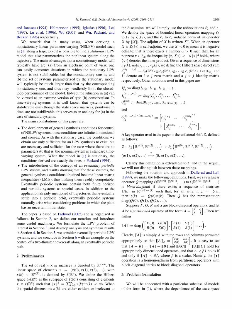
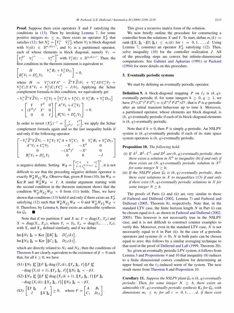
Fig. 1. Two Thruster Hovercraft.

positive definite solutions satisfying the synthesis conditions(S1–S3) for all k = 0, 1, . . . , N + q − 1, with Xs(N + q) =

Xs(N ) and Ys(N + q) = Ys(N ).

Solutions X and Y can be used to construct an (N , q)-eventually periodic controller Kδ . We remark that it may bepossible to construct from these solutions an (M, q)-eventuallyperiodic controller, where h ≤ M ≤ N , as suggested byPart (i) of Proposition 10. Note that generally we seek a γ -admissible synthesis, namely one that guarantees closed-loopstability as well as the norm condition ‖w 7→ z‖ < γ for someγ . Clearly, a γ -admissible synthesis for Gδ is a 1-admissiblesynthesis for Gδ , where Gδ has the same realization as Gδexcept that C1s =

1γ

C1s , C1p =1γ

C1p, D11 =1γ

D11, and

D12 =1γ

D12, and so, the previous synthesis results are stillapplicable in this case. Furthermore, by employing the Schurcomplement formula, it is possible to ensure that the synthesisconditions are also linear in γ (or γ 2 as in Farhood and Dullerud(2005, Problem (16))) and hence transform the synthesisfeasibility problem into a convex optimization one to find theminimum γ .

6. Example: Control of a two-thruster hovercraft

We now apply the NSLPV approach to control a two-thruster hovercraft along an eventually periodic trajectory. Thishovercraft, shown in Fig. 1, floats on an air cushion caused by acontinuous air flow through a perforated sheet underneath it.This causes the hovercraft to glide on an almost frictionlesssurface. The two thrusters are positioned equidistantly from thecentral axis of the craft, where L = 0.15 m. These thrusterscan only push in the forward direction, and each can exert aforce of at most 2.5 Newtons. Following are the translationaland rotational data for this system: mass m = 1.731 kg,translational friction bt = 3.7×10−3 N s/m, rotational frictionbr = 3.65 × 10−4 N s m/rad, and polar moment of inertiaI = 2.36328 × 10−2kg m2.

6.1. Nonlinear model and reference trajectory

Appealing to the free-body diagram in Fig. 1, the equationsof motion for the hovercraft are given by

mx + bt x = (u1 + u2) cos θ, (14)

my + bt y = (u1 + u2) sin θ, (15)

I θ + br θ = (u2 − u1)L . (16)

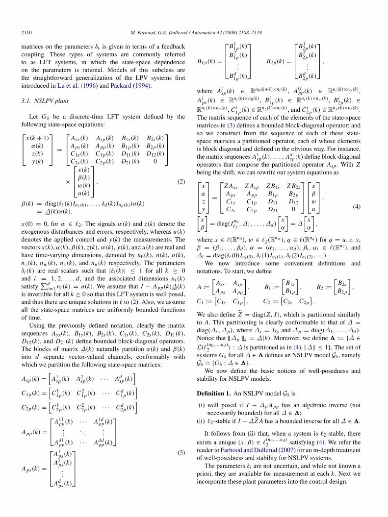
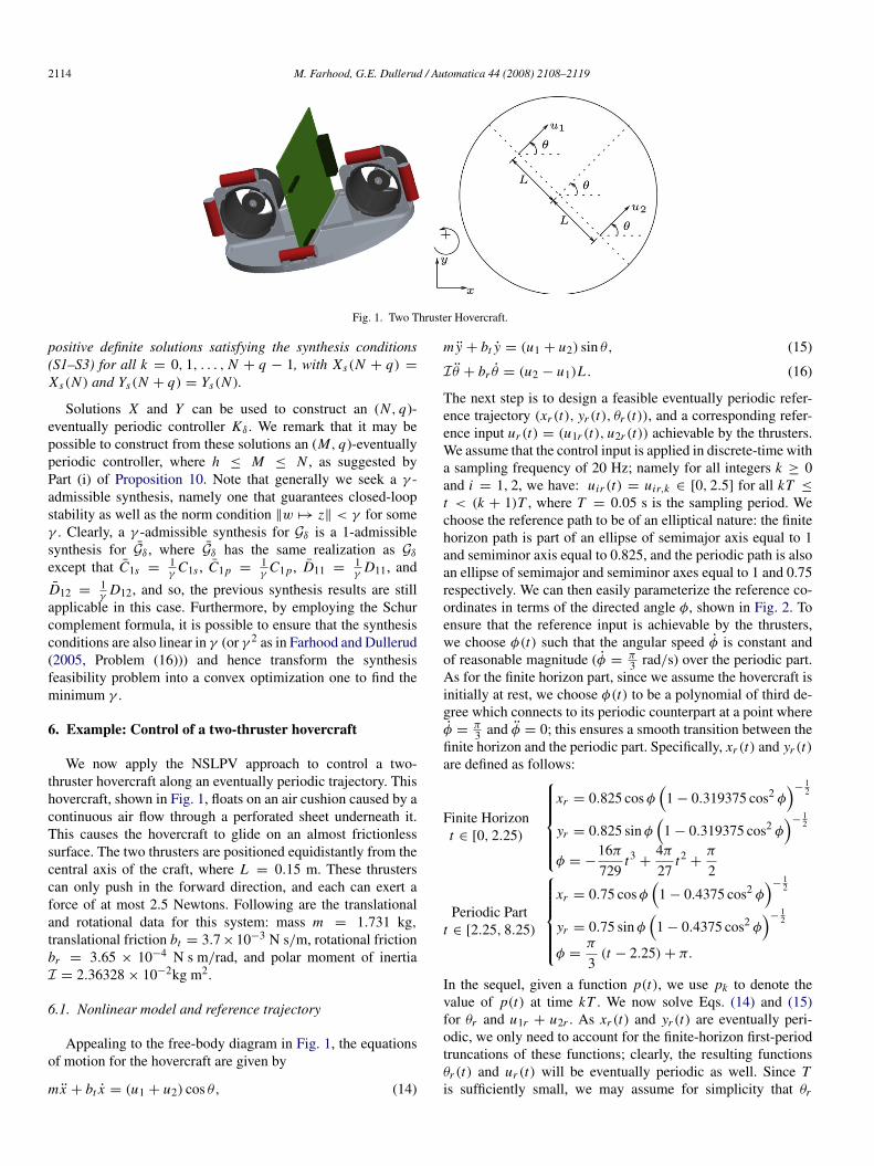
The next step is to design a feasible eventually periodic refer-ence trajectory (xr (t), yr (t), θr (t)), and a corresponding refer-ence input ur (t) = (u1r (t), u2r (t)) achievable by the thrusters.We assume that the control input is applied in discrete-time witha sampling frequency of 20 Hz; namely for all integers k ≥ 0and i = 1, 2, we have: uir (t) = uir,k ∈ [0, 2.5] for all kT ≤

t < (k + 1)T , where T = 0.05 s is the sampling period. Wechoose the reference path to be of an elliptical nature: the finitehorizon path is part of an ellipse of semimajor axis equal to 1and semiminor axis equal to 0.825, and the periodic path is alsoan ellipse of semimajor and semiminor axes equal to 1 and 0.75respectively. We can then easily parameterize the reference co-ordinates in terms of the directed angle φ, shown in Fig. 2. Toensure that the reference input is achievable by the thrusters,we choose φ(t) such that the angular speed φ is constant andof reasonable magnitude (φ =

π3 rad/s) over the periodic part.

As for the finite horizon part, since we assume the hovercraft isinitially at rest, we choose φ(t) to be a polynomial of third de-gree which connects to its periodic counterpart at a point whereφ =

π3 and φ = 0; this ensures a smooth transition between the

finite horizon and the periodic part. Specifically, xr (t) and yr (t)are defined as follows:

Finite Horizont ∈ [0, 2.25)

xr = 0.825 cosφ

(1 − 0.319375 cos2 φ

)−12

yr = 0.825 sinφ(

1 − 0.319375 cos2 φ)−

12

φ = −16π729

t3+

4π27

t2+π

2

Periodic Partt ∈ [2.25, 8.25)

xr = 0.75 cosφ

(1 − 0.4375 cos2 φ

)−12

yr = 0.75 sinφ(

1 − 0.4375 cos2 φ)−

12

φ =π

3(t − 2.25)+ π.

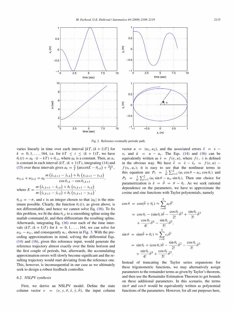
In the sequel, given a function p(t), we use pk to denote thevalue of p(t) at time kT . We now solve Eqs. (14) and (15)for θr and u1r + u2r . As xr (t) and yr (t) are eventually peri-odic, we only need to account for the finite-horizon first-periodtruncations of these functions; clearly, the resulting functionsθr (t) and ur (t) will be eventually periodic as well. Since Tis sufficiently small, we may assume for simplicity that θr

M. Farhood, G.E. Dullerud / Automatica 44 (2008) 2108–2119 2115

Fig. 2. Reference eventually periodic path.

varies linearly in time over each interval [kT, (k + 1)T ] fork = 0, 1, . . . , 164, i.e. for kT ≤ t ≤ (k + 1)T , we haveθr (t) = ak · (t − kT )+ θr,k , where ak is a constant. Then, as uris constant in each interval (kT, (k + 1)T ), integrating (14) and(15) over these intervals gives ak =

2T

(arccotE − θr,k

)+

2επT ,

u1r,k + u2r,k = akm

(yr,k+1 − yr,k

)+ bt

(yr,k+1 − yr,k

)cos θr,k − cos θr,k+1

,

where E =m

(xr,k+1 − xr,k

)+ bt

(xr,k+1 − xr,k

)m

(yr,k+1 − yr,k

)+ bt

(yr,k+1 − yr,k

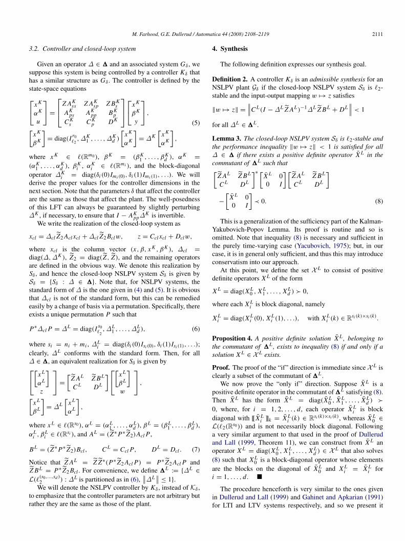
) ,θr,0 = −π , and ε is an integer chosen so that |ak | is the min-imum possible. Clearly, the function θr (t), as given above, isnot differentiable, and hence we cannot solve Eq. (16). To fixthis problem, we fit the data θr,k to a smoothing spline using thematlab command fit, and then differentiate the resulting spline.Afterwards, integrating Eq. (16) over each of the time inter-vals (kT, (k + 1)T ) for k = 0, 1, . . . , 164, we can solve foru2r − u1r , and consequently ur , shown in Fig. 3. With the pre-ceding approximations in mind, solving the differential Eqs.(14) and (16), given this reference input, would generate thereference trajectory almost exactly over the finite horizon andthe first couple of periods, but, afterwards, the accumulatingapproximation errors will slowly become significant and the re-sulting trajectory would start deviating from the reference one.This, however, is inconsequential in our case as we ultimatelyseek to design a robust feedback controller.

6.2. NSLPV synthesis

First, we derive an NSLPV model. Define the statecolumn vector v = (x, y, θ, x, y, θ ), the input column

vector u = (u1, u2), and the associated errors v = v −

vr and u = u − ur . The Eqs. (14) and (16) can beequivalently written as v = f (v, u), where f (·, ·) is definedin the obvious way. We have ˙v = v − vr = f (v, u) −

f (vr , ur ); it is easy to see that the nonlinear terms inthis equation are P1 =

1m

∑2i=1 (ui cos θ − uir cos θr ) and

P2 =1m

∑2i=1 (ui sin θ − uir sin θr ). Then one choice for

parametrization is δ = θ = θ − θr . As we seek rationaldependence on the parameters, we have to approximate thecosine and sine functions with Taylor polynomials, namely

cos θ = cos(θ + θr ) ≈

5∑i=0

ai θi

= cos θr − (sin θr )θ −cos θr

2!θ2

+sin θr

3!θ3

+cos θr

4!θ4

−sin θr

5!θ5,

sin θ = sin(θ + θr ) ≈

5∑i=0

ci θi

= sin θr + (cos θr )θ −sin θr

2!θ2

−cos θr

3!θ3

+sin θr

4!θ4

+cos θr

5!θ5.

Instead of truncating the Taylor series expansions forthese trigonometric functions, we may alternatively assignparameters to the remainder terms as given by Taylor’s theorem,and then use the Remainder Estimation Theorem to get boundson these additional parameters. In this scenario, the termssin θ and cos θ would be equivalently written as polynomialfunctions of the parameters. However, for all our purposes here,

2116 M. Farhood, G.E. Dullerud / Automatica 44 (2008) 2108–2119

Fig. 3. Reference angle θ and control input.

such a parametrization needlessly complicates the resultingNSLPV model. Now, some algebra leads to

P1 ≈ ψ1(θ , t)θ +[ψ2(θ , t) ψ2(θ , t)

]u,

P2 ≈ ρ1(θ , t)θ +[ρ2(θ , t) ρ2(θ , t)

]u,

where ψ1(θ , t) =∑4

j=0 κ j θj , ψ2(θ , t) =

∑5j=0 λ j θ

j ,

ρ1(θ , t) =∑4

j=0 µ j θj , ρ2(θ , t) =

∑5j=0 ξ j θ

j , λ j =a jm ,

κ j =u1r +u2r

m a j+1, ξ j =c jm , and µ j =

u1r +u2rm c j+1.

As a result, we get the continuous-time state-space equation:

˙v = A(θ , t)v + B(θ , t)u, (17)

where A(θ , t) and B(θ , t) are equal to

03×3 I30 0 ψ1(θ , t)0 0 ρ1(θ , t)0 0 0

−bt

m0 0

0 −bt

m0

0 0 −br

I

and

03×2ψ2(θ , t) ψ2(θ , t)

ρ2(θ , t) ρ2(θ , t)

−L

IL

I

,

respectively. Next, we formulate this equation in an LFTframework. We will find the following notation convenient:

δ I ?M = M21(I − δM11)−1δM12 +M22,

where M = .

Our goal is to equivalently present state-space equation (17) inthe following LFT format:

˙v = Acss(t)v + Ac

sp(t)βc + Bc2s(t)u,

αc = Acps(t)v + Ac

pp(t)βc + Bc2p(t)u, βc = θαc.

In other words, we need to write the matrix-valued functionsA(θ , t) and B(θ , t) as

θ I ? and θ I ? , (18)

respectively. It is not difficult to see that

A(θ , t) = θ I4 ? = θ I4 ?

and B(θ , t) = θ I5 ? = θ I5 ? ,

where E0 =[0 0 1 0 0 0

], F0 =

[1 1

],

E1 =

κ1 κ2 κ3 κ4µ1 µ2 µ3 µ40 0 0 0

,

M. Farhood, G.E. Dullerud / Automatica 44 (2008) 2108–2119 2117

E2 =

0 0 κ0 −

bt

m0 0

0 0 µ0 0 −bt

m0

0 0 0 0 0 −br

I

,

F1 =

λ1 λ2 λ3 λ4 λ5ξ1 ξ2 ξ3 ξ4 ξ50 0 0 0 0

, F2 =

λ0 λ0ξ0 ξ0

−L

IL

I

.It is obvious from the preceding that the matrix-valued systemfunctions in (18) can be chosen as follows:

Acpp =

[A11 0

0 B11

], Ac

ps =

[A12

0

], Bc

2p =

[0B12

],

Acsp(t) =

[A21 B21

],

Acss(t) = A22, Bc

2s(t) = B22.

In order to simplify the discretization of the continuous-timeLFT model, and since the sampling period T is sufficientlysmall, it is reasonable to assume that the scheduled parameter δvaries very slowly in time interval [kT, (k +1)T ) that its valueson this interval can be approximated by δk = θ (kT ). Then,we can use zero-order hold sampling to obtain the followingdiscrete-time state-space equation:

vk+1 = Ass,k vk + Asp,kβk + B1s,kwk + B2s,k uk,

where Ass,k = Φss ((k + 1)T, kT ), Φss being the statetransition matrix associated with Ac

ss(t), vk = v(kT ), βk =

βc(kT ), Asp,k =∫ (k+1)T

kT Φss ((k + 1)T, τ ) Acsp(τ )dτ , Bis,k =∫ (k+1)T

kT Φss ((k + 1)T, τ ) Bcis(τ )dτ for i = 1, 2, with Bc

1s =[03×3 I3

]∗ (i.e. the disturbances w are in the form of torquesas well as forces in the x and y directions, applied like theinput in discrete time with a sampling frequency of 20 Hz).Alternatively, as proposed in Apkarian (1997), we can use abilinear transformation to obtain a discrete-time trapezoidalapproximation.

We assume that the parameter δ = θ is such that |δ| ≤π6 .

Then, this bound is absorbed into the plant so that the newscaled parameter δ satisfies |δ| ≤ 1, where δ =

π6 δ. Also, due to

this scaling, we get Aps =π6 Ac

ps , App =π6 Ac

pp, B1p =π6 Bc

1p,B2p =

π6 Bc

2p. We assume that the states x , y, and θ are exactlymeasurable, and as for the exogenous errors to be controlled,we choose to equally penalize x , y, θ , u1, and u2. Then, weget the discrete-time (45, 120)-eventually periodic LPV model:βk = δkαk, |δk | ≤ 1,vk+1αkzkpk

=

Ass,k Asp,k B1s,k B2s,kAps App B1p B2pC1s C1p D11 D12C2s C2p D21 D22

vkβkwkuk

, (19)

where w ∈ `2, v(0) = 0, B1p, C1p, C2p, D11, D21, D22 are allzero matrices, and C1s = diag(I3, 02×3),

C2s =[I3 03×3

], D12 =

[02×3 I2

]∗.

The LFT formulation has significantly increased the modeldimensions; we now have six states as well as nine copies of

the parameter δ. Clearly, a model reduction theory for such LFTmodels is important, and this is treated in-depth in Farhood andDullerud (2007). In this case, however, since the minimalitytheory for transfer functions in a single complex variable isidentical to that for rational functions in a single real variable,we can reduce the model dimensions pointwise in time at nocost. Specifically, appealing to (19), we have

vk+1 =

vkwkuk

,and so, at each k, we can reduce the dimensions of the modelby eliminating any uncontrollable or unobservable states of thereal variable “transfer function” H

(δk

), and hence obtaining

the minimal realization of H(δk

). Doing so, we end up with a

reduced LFT model with six states and five copies of δ at eachtime instant.

Appealing to Corollary 11 and its subsequent discussion, wecan solve for a γmin-admissible (45, 120)-eventually periodicLPV synthesis Kδ , where γmin is the minimum achievable γ bysuch a synthesis. Using SeDuMi (Sturm, 1999), we find that,in this case, γmin ≈ 2.57, whereas in the counterpart LTVcase (i.e. no parameters) its value would be about 2. Clearly,as the bound on the parameter θ decreases, the value of γminpotentially decreases too, but it may not in general converge tothe corresponding LTV value.

6.3. Simulation

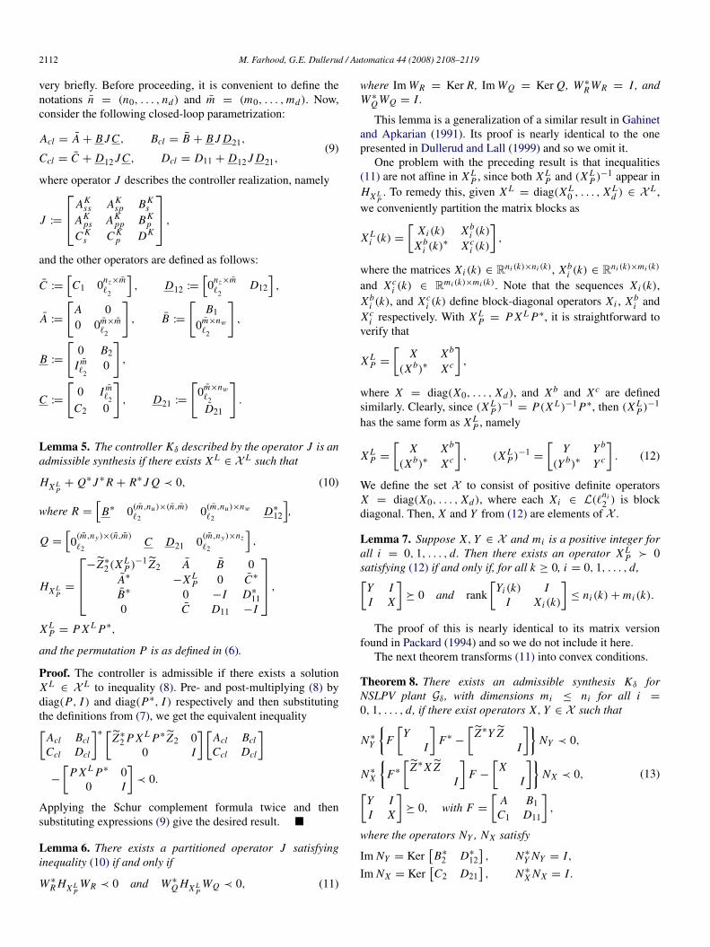
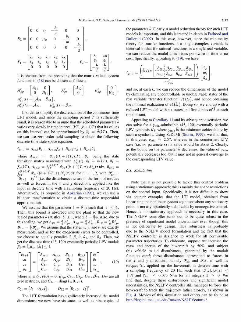
Note that it is not possible to tackle this control problemusing a stationary approach; this is mainly due to the restrictionson the control input. Specifically, it is not difficult to showvia counter examples that the LTI model, obtained fromlinearizing the nonlinear system equations about any stationarypoint, is not asymptotically stabilizable by nonnegative control.Hence, a nonstationary approach is necessary in this case.The NSLPV controller turns out to be quite robust in thepresence of significant model uncertainties even though thisis not deliberate by design. This robustness is probablydue to the NSLPV model formulation and the fact that theNSLPV controller is designed to work for all permissibleparameter trajectories. To elaborate, suppose we increase themass and inertia of the hovercraft by 50%, and subjectthis vehicle to iid disturbances, generated by the matlabfunction rand; these disturbances correspond to forces inthe x and y directions, namely Fxk and Fyk , as well astorques Tk , applied on the hovercraft in discrete-time witha sampling frequency of 20 Hz, such that |Fxk |, |Fyk | ≤

1 N and |Tk | ≤ 0.075 N m for all integers k ≥ 0. Wefind that, despite these disturbances and significant modeluncertainties, the NSLPV controller still manages to force thehovercraft to track the trajectory rather closely, as shown inFig. 4. Movies of this simulation and others can be found athttp://legend.me.uiuc.edu/˜mazen/NSLPVcontrol/.

2118 M. Farhood, G.E. Dullerud / Automatica 44 (2008) 2108–2119

Fig. 4. NSLPV simulation (dashed curves correspond to reference).

7. Conclusions

This paper gives results for the control of nonstationaryLPV systems, which are analogous to those for stationary LPVsystems. The motivation for this work is a systematic methodfor gain scheduling of systems controlled along prespecifiedtrajectories. In this context a benefit of using a nonstationarymodel is to reduce the conservatism introduced when capturingthe behaviour of a nonlinear system in an LPV model.

References

Apkarian, P. (1997). On the discretization of LMI-synthesized linear parameter-varying controllers. Automatica, 33, 655–661.

Apkarian, P., & Gahinet, P. (1995). A convex characterization of gain-scheduled H∞ controllers. IEEE Transactions on Automatic Control, 40,853–864.

Ball, J. A., Gohberg, I., & Kaashoek, M. A. (1992). Nevanlinna-pickinterpolation for time-varying input-output maps: The discrete case.In Operator theory: Advances and applications: Vol. 56. Time-variantsystems and interpolation (pp. 1–51). Basel: Birkhauser.

Dullerud, G. E., & Lall, S. G. (1999). A new approach to analysis and synthesisof time-varying systems. IEEE Transactions on Automatic Control, 44(8),1486–1497.

Farhood, M. (2005). A semidefinite programming approach for control ofsystems along trajectories. Ph.D. thesis, Department of Mechanical andIndustrial Engineering, University of Illinois at Urbana-Champaign.

Farhood, M., & Dullerud, G. E. (2002). LMI tools for eventually periodicsystems. Systems and Control Letters, 47(5), 417–432.

Farhood, M., & Dullerud, G. E. (2005). Duality and eventually periodicsystems. International Journal of Robust and Nonlinear Control, 15(13),575–599.

Farhood, M., & Dullerud, G. E. (2007). Model reduction of nonstationary LPVsystems. IEEE Transactions on Automatic Control, 52(2), 181–196.

Gahinet, P., & Apkarian, P. (1991). A linear matrix inequality approach toH∞ control. International Journal of Robust and Nonlinear Control, 4,421–448.

Halanay, A., & Ionescu, V. (1994). Time-varying discrete linear systems.Birkhauser.

Helmersson, A. (1995). Methods for robust gain scheduling. Ph.D. thesis,Department of Electrical Engineering, Linkoping University, Linkoping,Sweden.

Iglesias, P. A. (1996). An entropy formula for time-varying discrete-time control systems. SIAM Journal on Control and Optimization, 34,1691–1706.

Lee, L. H. (1997). Identification and robust control of linear parameter-varyingsystems. Ph.D. thesis, Department of Mechanical Engineering, Universityof California at Berkeley.

Lu, W. M., Zhou, K., & Doyle, J. C. (1996). Stabilization of uncertain linearsystems: An LFT approach. IEEE Transactions on Automatic Control, 41,50–65.

Packard, A. (1994). Gain scheduling via linear fractional transformations.Systems and Control Letters, 22, 79–92.

Sturm, J. F. (1999). Using SeDuMi 1.02, a MATLAB toolbox for optimizationover symmetric cones. Optimization Methods and Software, 11–12,625–653.

Wu, F. (2001). A generalized LPV system analysis and control synthesisframework. International Journal of Control, 74(7), 745–759.

Wu, F., Packard, A., & Becker, G. (1996). Induced L2-norm control for LPVsystems with bounded parameter variation rates. International Journal ofRobust and Nonlinear Control, 6, 983–998.

Yacubovich, V. A. (1975). A frequency theorem for the case in which the stateand control spaces are Hilbert spaces with an application to some problemsof synthesis of optimal controls. Sibirskii Matematicheskii Zhurnal, 15,639–668. English translation in Siberian Mathematics Journal.

Mazen Farhood received his bachelor’s degree inMechanical Engineering from the American Universityof Beirut, Lebanon, in 1999. He received the M.S.degree in 2001, and the Ph.D. degree in 2005, both inMechanical Engineering from the University of Illinoisat Urbana-Champaign. From Sept. 2006 to Oct. 2007,he was a postdoctoral fellow in the School of AerospaceEngineering at Georgia Institute of Technology. He iscurrently a scientific researcher in the Delft Center forSystems and Control, Delft University of Technology,

The Netherlands. His areas of current research interest include distributedcontrol, controlled maneuvers and tracking along trajectories, semidefiniteprogramming, model reduction and control of agile aerial vehicles.

M. Farhood, G.E. Dullerud / Automatica 44 (2008) 2108–2119 2119

Geir E. Dullerud was born in Oslo, Norway, in1966. He received the BASc degree in EngineeringScience, in 1988, and the MASc degree in ElectricalEngineering, in 1990, both from the University ofToronto, Canada. In 1994 he received his Ph.D.in Engineering from the University of Cambridge,England.

Since 1998 he has been a faculty member inMechanical Engineering at the University of Illinois,Urbana-Champaign, where he is currently Professor.

From 1996 to 1998 he was an assistant professor in Applied Mathematics atthe University of Waterloo, Canada. During 1994 and 1995 he was a ResearchFellow and Lecturer at the California Institute of Technology, in the Controland Dynamic Systems Department. He has published two books: Control ofUncertain Sampled-data Systems, Birkhauser 1996, and A Course in RobustControl Theory (with F. Paganini), Texts in Applied Mathematics, Springer,2000. His areas of current research interest include networks, complex andhybrid dynamic systems, and control of distributed robotic systems. He receivedthe Xerox Award at UIUC in 2005, and the National Science FoundationCAREER Award in 1999.