Embed Size (px)
Citation preview

Nonparametric Nonstationary
Regression
Inauguraldissertation
zur Erlangung des akademischen Grades
eines Doktors der Wirtschaftswissenschaften
der Universitat Mannheim
vorgelegt von
Melanie Schienle
Marz 2008

Abteilungssprecher: Prof. Hans-Peter Gruner, Ph.D.
Referent: Prof. Dr. Enno Mammen
Korreferent: Prof. Oliver Linton, Ph.D.
Tag der Verteidigung: Freitag, 13.06.2008

Acknowledgements
First of all, I wish to thank my advisor Enno Mammen for his guidance and su-
pervision of my thesis. He introduced me to the topic of nonparametric regression
and my research has benefited a lot from his broad statistical knowledge. I am
very grateful for his support and confidence in me.
I also wish to thank Oliver Linton for advice on my thesis and beyond. I benefited
a lot from three very encouraging and insightful months in London. Numerous dis-
cussions not only broadened my perspective on my own topic but on econometrics
in general.
Kyusang Yu was an invaluable support in my struggle with technical details. I
benefited a lot not only from his experience with nonparametric statistics but also
from uncountably many lunch box apples and clementines.
During the time at the Chair of Statistics I have enjoyed working with my col-
leagues Christian Conrad, Berthold Haag, Christoph Rothe and Christoph Nagel.
It was always pleasant and fruitful to discuss scientific questions or anything else.
I also wish to thank my fellows at the CDSEM – in particular the mensa crew. I
enjoyed the lively atmosphere and the stimulating research environment.
I am especially grateful to my Stephan for still liking me.
Mannheim, March 28th, 2008
Melanie Schienle


Contents
1 Introduction 1
1.1 Relevance and Literature . . . . . . . . . . . . . . . . . . . . . . . . 1
1.2 Model and Approach . . . . . . . . . . . . . . . . . . . . . . . . . . 4
1.3 Main Results . . . . . . . . . . . . . . . . . . . . . . . . . . . . . . 5
1.4 Outline . . . . . . . . . . . . . . . . . . . . . . . . . . . . . . . . . . 8
2 Motivation and Basic Framework 11
2.1 Motivation, Intuition and Some Notation . . . . . . . . . . . . . . . 11
2.1.1 Small Sets and Feller Chains . . . . . . . . . . . . . . . . . . 12
2.1.2 β–null Harris Recurrence . . . . . . . . . . . . . . . . . . . . 14
2.1.3 Nonparametric Curse of Dimensionality . . . . . . . . . . . . 20
2.2 Nonparametric Kernel Estimators . . . . . . . . . . . . . . . . . . . 21
3 Estimation 29
3.1 Choice of the Type of Estimation Technique . . . . . . . . . . . . . 29
3.2 Standard Smooth Backfitting for Nonstationary Covariates . . . . . 31
3.3 Generalized Smooth Backfitting (GSBE) . . . . . . . . . . . . . . . 33
3.3.1 GSBE for Pairwise β–null Harris Recurrent Covariates . . . 33
3.3.2 Adapted GSBE for γ–wise β–null Harris Recurrent Covariates 36
4 Asymptotic Results 39
4.1 Standard Smooth Backfitting for Nonstationary Covariates . . . . . 40
4.2 GSBE . . . . . . . . . . . . . . . . . . . . . . . . . . . . . . . . . . 48
vi CONTENTS
4.3 Extensions . . . . . . . . . . . . . . . . . . . . . . . . . . . . . . . . 54
4.3.1 Adapted GSBE to γ–wise β–null Harris Recurrence . . . . . 54
4.3.2 Asymptotic Independence . . . . . . . . . . . . . . . . . . . 57
4.4 Remarks on Oracle Efficiency . . . . . . . . . . . . . . . . . . . . . 63
5 Finite Sample Behavior: A Simple Simulation Study 67
6 Conclusion 75
6.1 Summary . . . . . . . . . . . . . . . . . . . . . . . . . . . . . . . . 75
6.2 Outlook . . . . . . . . . . . . . . . . . . . . . . . . . . . . . . . . . 76
A Appendix 79
A.1 Markov Theory . . . . . . . . . . . . . . . . . . . . . . . . . . . . . 79
A.1.1 Split Chain and Invariant Measure . . . . . . . . . . . . . . 79
A.1.2 β–null Harris recurrence . . . . . . . . . . . . . . . . . . . . 81
A.1.3 The Quotient Limit Theorem . . . . . . . . . . . . . . . . . 82
A.2 Proofs . . . . . . . . . . . . . . . . . . . . . . . . . . . . . . . . . . 82
A.2.1 On the Structural Form of Generalized Smooth Backfitting . 82
A.2.2 Preliminary Lemmata . . . . . . . . . . . . . . . . . . . . . 85
A.2.3 Proofs of the Theorems . . . . . . . . . . . . . . . . . . . . . 99
Bibliography 112
Chapter 1
Introduction
This thesis studies nonparametric estimation techniques for a general regression
set–up under very weak conditions on the covariate process. In particular, regres-
sors are allowed to be high–dimensional stochastically nonstationary processes.
The concept of nonstationarity comprises time series observations of random walk
or long memory type. Admissible processes might “wander off”, but recur any
time they do so. We introduce the first kernel type estimation method for such
nonstationary regressors without restricting their dimension. This set–up is moti-
vated by and generalizes approaches in parametric econometric time series analysis
with nonstationary components. It offers a possible way to extend and test for
linear cointegration.
1.1 Relevance and Literature
There is substantial empirical evidence that many important economic factors
without a deterministic time trend such as real consumer prices, individual con-
sumption, exchange rates, and real GDP are stochastically nonstationary (See e.g.
Meese and Singleton [1982], Kwiatkowski et al. [1992], or Sun and Phillips [2004]).
In Econometric time series literature, though, the study of such nonstationary
time series has been dominated by parametric models. Most commonly, stochasti-
cally nonstationary processes are modeled as integrated or fractionally integrated
2 Chapter 1. Introduction
(see the extensive literature on unit root processes started with Dickey and Fuller
[1979] for purely integrated and Phillips [1987] for general ARIMA models; for
fractionally integrated models see Baillie [1996] for a survey and e.g. Diebold and
Rudebusch [1999] among others). For valid inference, though, the decision for a
nonstationary model as opposed to a stationary one must be correct (tests for
unit root can be found in Dickey and Fuller [1981], Phillips and Perron [1988]
or for stationarity against unit root in Kwiatkowski et al. [1992]). In regression
models, structural relationships between nonstationary variables have been exten-
sively studied in the context of cointegration. Introduced in Engle and Granger
[1987], stochastically nonstationary time series are cointegrated if there exists a
linear combination such that the residual is I(0) an thus mostly stationary. This
linear type of cointegration can be easily tested for , e.g. as proposed by Johansen
[1991]. Nonlinear extensions as e.g. in Granger and Hallman [1991], Park and
Phillips [1999], Park and Phillips [2001], or de Jong and Wang [2005] are still rare
in the applied literature as they appear restrictive in fitting a specific parametric
relationship which is hard to test for (see Hong and Phillips [2005]). While eco-
nomic theory often suggests nonlinear responses (see e.g Lewbel and Ng [2005] in
demand), it is often not explicit regarding the functional form (see e.g.Meese and
Rose [1991] for exchange rates). Therefore the simplicity of econometric analysis
so far is not due to simple true models but due to lack of respective more general
tools. There is need for appropriate nonparametric methods in this general setting.
In nonparametric regression the full form of the functional relation between a
response variable and observables is determined from the data. This is in contrast
to parametric models where a global parametric form is prespecified up to a finite
dimensional parameter which is obtained by estimation. In particular, for kernel
type nonparametric estimation techniques we derive point estimates of the struc-
tural relationship by local weighted averages of observations in the neighborhood of
the point of interest. Though for nonparametric estimation to be possible, the vast
class of nonstationary processes is too wide and general comprising deterministic
trends as well as stochastic nonstationarities. In order to apply local smoothing
techniques in the state space, however, the processes cannot “wander off for good”
1.1 Relevance and Literature 3
with a deterministic trend, but they must recur to any point in their range almost
surely guaranteeing sufficiently many observations for inference. This intuitive
and natural property can be formalized as Harris recurrence – a concept from
Markov chain literature. It relaxes usual stationarity and ergodicity assumptions
but allows for stochastic nonstationarity as of random walk type. Therefore it is
the appropriate framework for nonstationary kernel type inference. While Harris
recurrence puts a restriction on the behavior of the time series in the state domain,
it is more general than assumptions in the time domain such as local stationarity
or mixing, which require a certain alignment of the observed processes in time (For
nonparametric nonstationary estimation in the class locally stationary processes
via spectral density approximations see Dahlhaus [1997] and the rich literature
thereafter)
The idea of Harris recurrence as the key minimal assumption for valid kernel re-
gression techniques with Markov processes was first suggested by Yakowitz [1989].
His analysis, though, was restricted to the positive recurrent case and provided only
consistency results for nearest neighbor estimates in this setting. Phillips and Park
[1998] were the first to move towards possibly null recurrent processes. They used
local time arguments, but their results only applied to one dimensional first order
unit autoregressions. Independently Moloche [2001] and Karlsen and Tjøstheim
[2001] have introduced an estimation framework for regression with general null
Harris recurrent Markov processes. While the first uses embedding techniques,
that require restrictive assumptions and employs existing results from probability
theory literature, the later is more general with different direct techniques. Within
the imperceptibly smaller class of β–null Harris recurrent processes, Karlsen and
Tjøstheim [2001] provide results on consistency and derive asymptotic normality
by inverting a stable recurrence time process. The type of nonstationarity of the
data is captured by a single parameter β, the degree of regular variation in the
tails of the recurrence time process. It also represents the polynomial degree of
the expected stochastic rates of convergence and therefore offers an important way
to compare the nonstationary results to well–known stationary theorems. A com-
parison of the two strains of literature is contained in Bandi [2004]. In general,
4 Chapter 1. Introduction
the literature on nonparametric nonstationary estimation is still quite new and
therefore scarce. Lately there are some papers following the local time approach
such as Bandi and Phillips [2003] and Bandi [2004] studying nonstationary dif-
fusions and Wang and Phillips [2006] with general cointegration type estimation.
Though a partial linear model is examined in Chen et al. [2007] under β–null Harris
recurrence. We also employ the β–null Harris recurrence framework.
In general, however, high–dimensional nonparametric estimation suffers from
standard curse of dimensionality (COD). The more regressors are included the
worse the finite sample behavior. For nonstationary data, in particular, this can
lead to extremely slow rates of convergence, requiring very large sample sizes
for significant results. Furthermore in the nonstationary setting, an additional
even more severe nonstationary curse of dimensionality complicates nonparametric
estimation. For dimensions larger than two, Harris recurrence of joint regressors
is restrictive. In fact, the more regressors are added, the more “unlikely” it is
for the compound process to still fit the framework of Harris recurrence. Most
prominently, a random walk is Harris recurrent only up to dimension two and
transient for any higher dimension. In such cases, the performance of existing
procedures of Karlsen et al. [2007] and Moloche [2001] does not only deteriorate,
but none of them can be applied at all. There is no existing nonparametric method
for such high–dimensional regression in this general setting.
1.2 Model and Approach
In this work, we provide an estimation method which countervails both curses
of dimensionality. To overcome the first, ordinary COD, an additive model is
estimated. In the stationary mixing case, additive models have provided a powerful
technique to overcome this problem and to still maintain high model flexibility.
Denote observations by subscripts and dimension components by superscripts. In
the entire thesis we use the short–hand notation Xjk = (Xj, Xk). Then given a
random design of n joint observations of (X, Y ) ∈ Rd×R, we estimate an additive
conditional mean function m : Rd → R with component functions mj : R → R for
1.3 Main Results 5
j = 1, . . . , d and scalar m0 by
Yi = m0 +d∑
j=1
mj(Xji ) + εi for all i ∈ {1, . . . , n} (1.1)
under suitable identification conditions for mj, j = 1, . . . , d. We always assume
there is no concurvity, i.e. for m1, . . . ,md nontrivial we cannot have m1(x1) +
· · ·+md(xd) = 0 for all (x1, . . . , xd). The response Y and at least all univariate Xj
and pairs of bivariate marginal components Xjk of the covariate vector X belong
to a specific class of Markov processes, β–null Harris recurrent processes, which
is wide and general enough to include stationary and a wide range nonstationary
processes.
In order to tackle the second nonstationary COD, however, an estimation method
for the additive model must rely on low dimensional components only - at best only
univariate and bivariate ones to include the widest possible class of processes. In a
stationary setting, smooth backfitting introduced by Mammen et al. [1999] fulfills
these requirements as it does not need a full–dimensional estimate in any step
of the method. On this basis, we develop and introduce the generalized smooth
backfitting procedure for a general nonstationary setting.
1.3 Main Results
The main contributions of this thesis are the following. They are stated in order
of importance which does not correspond to their order of appearance in the text.
First nonparametric technique for high–dimensional nonstationary re-
gression
With generalized smooth backfitting we introduce the first valid nonparametric es-
timation method under weakest assumptions on multidimensional covariates. The
essential requirement is only pairwise β–null Harris recurrence which comprises
a significantly larger class of important practical processes than the class of full
β–null Harris recurrent processes where other existing estimation procedures are
6 Chapter 1. Introduction
restricted to (see Karlsen et al. [2007]). Therefore it offers a first way to countervail
both, the standard curse of dimensionality but also the more severe nonstation-
ary curse of dimensionality. The generality in type of underlying data, however,
restricts admissible model classes to at most pairwise additive. This implies that
generalized smooth backfitting only yields the best additive fit if the true model is
additive or pairwise additive as in (3.9). For more general true models this is not
guaranteed. In the most general setting, identification is obtained under general-
ized conditional independence assumptions where the residual can also contain a
certain type of stochastic nonstationarity. The exact conditions are stated in As-
sumptions 4.4 and the most general residual form is mentioned in Remark 4 after
Theorem 4.3. We derive the asymptotic expansion of the generalized smooth back-
fitting estimators in Theorem 4.3. This is the main technical result of this thesis.
Components have a rate of convergence and variance of univariate type but gov-
erned by the worst case bivariate nonstationary type. Therefore convergence also
holds jointly for all component functions. In order to achieve asymptotic normal-
ity, the speed of convergence is stochastic due to the nonstationarity of the data.
Section 4.4 contains some considerations on oracle efficiency of the procedure.
First nonparametric estimation method for an additive conditional
mean function with nonstationary data
Depending on the degree of nonstationarity in the covariate vector, we introduce
estimation techniques for additive regression models in this general setting. The
more regressors are compoundly β–null Harris recurrent , say γ with 2 ≤ γ ≤ d
of them, the more general can the true underlying model be, to still obtain the
best additive fit in a projection sense via adapted generalized smooth backfitting.
Thus allowing for higher model generality, rates of convergence and variances are
governed by the worst case γ–wise nonstationary type in each component. The re-
spective method is presented in Section 3.3.2 and its asymptotic expansion is stated
in Theorem 4.5 under the weakest assumptions on the spacial correlation structure
of covariates and residual. It contains standard smooth backfitting (for γ = d) and
generalized smooth backfitting (for γ = 2) as extreme subcases. Adapted gener-
1.3 Main Results 7
alized smooth backfitting can yield the closest additive approximation to a fully
general true model only under full β–null Harris recurrence and standard smooth
backfitting. Asymptotic results for this case are stated in Section 3.2. Though
for generality in the fitted model class, the respective procedures lose in efficiency
with methods for increasing γ, by scaling according to higher dimensional types
of nonstationary data. This is briefly discussed in Section 4.4.
First nonparametric generalization of cointegration type models without
restricting the number of covariates
In the special subcase of ε being stationary mixing in (1.1), we estimate an additive
cointegration type relationship. In contrast to the existing more general nonpara-
metric approaches in Karlsen et al. [2007] and in Wang and Phillips [2006], however,
the number of cointegrated regressors is not restricted. Furthermore in order to
obtain the asymptotic results in Theorem 4.4 and Theorem 4.2 only structurally
simple and familiar moment type conditions must be satisfied, if covariates and
residual process satisfy a generalized spacial independence assumption.
These are the fundamental contributions of this thesis. Important secondary
aspects or extensions of the above results are highlighted in the following.
Stationary and nonstationary processes treated with same procedure
In the chosen framework, the presented estimation methods work irrespective of
underlying stationarity or not. While they are stated in the most general form
for nonstationary data, they contain the stationary case as a subcase. Thus other
than in parametric models, there is no pretesting for stationarity required. Our
methods are adaptive to stationarity or nonstationary data. Therefore in this
respect, there is no risk of model misspecification causing invalid inference.
Tailored Procedure for Stationary and Nonstationary covariates
In some high–dimensional economic models, in fact only one of the regressors ap-
pears as nonstationary while all others can be safely assumed as stationary (See e.g.
8 Chapter 1. Introduction
the study of Gil-Alana and Robinson [1997]). With such pre–knowledge about the
type of each regressor, we can improve on the efficiency of the general procedures
as suggested in Section 3.2 and 3.3. With an adapted method, we can estimate
stationary components at stationary rates. Therefore in finite sample studies and
in practice, the suggested tailored method offers a significant improvement under
feasibility aspects.
Uniform convergence results for β–null Harris recurrent processes
In order to show statistical properties of the generalized smooth backfitting estima-
tor, we establish uniform convergence results for density estimators and regression
estimators under the minimal assumption of β–null Harris recurrence. Due to the
lack of exponential inequalities of Bernstein or Hoeffding type in this general set-
ting, the proof of exponential tightness is quite lengthy and involved. As they are
new to the probability literature, Corollaries A.2.2 and A.3 deserve some attention
and might be of interest on their own.
1.4 Outline
This thesis is structured as follows. The second chapter presents the fundamental
framework for estimation and the basic form of local smoothers in this general set-
ting. In order to provide a thorough picture of the considered class of processes,
certain concepts and notations of Markov theory must be introduced. Though
the emphasis is on motivation and intuition how they facilitate our problem, while
some technical properties are included only in the Appendix. The focus is on β–null
Harris recurrence as the appropriate framework for kernel smoothing. Furthermore
form and properties of general multidimensional kernel estimators are discussed,
where features and specifics of the nonstationary setting are highlighted. With the
basic notions at hand, the subsequent third chapter introduces the new estimation
techniques. Depending on the degree of nonstationarity in the covariate process
and on how close an additive model is to true model, respective estimation strate-
gies are introduced. With generalized smooth backfitting we provide an estimation
1.4 Outline 9
procedure under the weakest assumptions on the covariates. Since it requires only
pairwise β–null Harris recurrence as minimal assumption, it is the first valid esti-
mation method for a vast class of high dimensional time series models. Chapter 4
contains the major convergence and asymptotic results. The focus is on the most
interesting asymptotic expansions in the case of full β–null Harris recurrence and
pairwise β–null Harris recurrence of the covariate vector. For completeness, inter-
mediate cases are briefly treated under Extensions. Furthermore two practically
interesting special cases are studied. We conclude the chapter by remarks on effi-
ciency. In the Chapter 5, a simple simulation study shows that the method works
in finite samples. the estimated five dimensional random walk model could not be
estimated by general existing methods. The last chapter sums up. As the studied
field of research is quite new, we conclude with an outlook for further research.
All proofs as well as major technicalities are contained in the Appendix, which
also comprises the formal statement of some basic notions and tools from Markov
theory.

10 Chapter 1. Introduction
Chapter 2
Motivation and Basic Framework
In this chapter we introduce necessary tools and concepts for conducting non-
parametric kernel type smoothing with stochastically nonstationary processes. In
particular, in the first section we study β–null Harris recurrent processes as the
appropriate framework for estimation. Series of discrete observations in this class
of processes comprise all strictly and weakly stationary as well as nonstationary
time series with potentially infinite, time dependent variance of unit root or long
memory type. For deriving certain stochastic properties and for a thorough un-
derstanding, some notions and results from Markov theory are needed. These are
presented with an emphasis on meaning and role of the employed techniques, while
technical details and exact definitions of most of the Markov chain properties can
be found in the Appendix. Comprehensive references for notions from Markov
theory are Meyn and Tweedie [1993] and Nummelin [1984]. Furthermore in the
second section, form and peculiarities of kernel estimators in this general setting
are examined. These are fundamental in Chapter 3 for establishing estimation
methods for an additive structural relationship as in (1.1).
2.1 Motivation, Intuition and Some Notation
Let {Xi}ni=1 be an aperiodic φ–irreducible Markov chain on the state space
(R,Bd
)with transition probability P . Let the region of estimation G = G1×. . .×Gd ⊆ R =
12 Chapter 2. Motivation and Basic Framework
R1× . . .×Rd ⊆ Rd be compact. Irreducibility essentially ensures that the Markov
chain does not degenerate to a subspace of the original space R. Technically it
implies that for any set A ∈ R with φ(A) > 0 it is∑
n P n(x, A) > 0 for any
starting point x ∈ R. Hence φ indicates, if a set can be reached by the process
or not. For inference, only sets of positive φ measure are of interest. Throughout
the paper, we assume that supp(φ) has non–empty interior1. Denote the class of
non–negative measurable functions with φ–positive support by E+. Then also a
set A ∈ R is in E+ if for the indicator function it is 1A ∈ E+.
It is not intrinsically natural that the process lives in a bounded set - though this
is inevitable for technical reasons in the estimation procedure. Note that G can
be chosen sufficiently large such that there are a sufficiently many data points
for nonparametric inference in G. Denote by ∂Gh the h ring boundary of G in
the following sense x ∈ ∂Gh iff ‖x− c‖ ≤ hC1 for any c from the boundary ∂G.
Furthermore write for the h ring interior Gh = inth(G) := G\∂Gh.
2.1.1 Small Sets and Feller Chains
To ease notation, we use the following short–hand notation: For any non–negative
measurable function η and any measure λ the operator kernel η⊗ λ is defined by:
η⊗ λ(x, A) := η(x)λ(A), for all (x, A) ∈ (Rn,Bn). For some general operator ker-
nel P denote: Pη(x) :=∫
AP (x, dy)η(y) is a function, λP (A) :=
∫Rn λ(dx)P (x, A)
is a measure and λPη(x, A) :=∫
A
∫Rn λ(dx)P (x, dy)η(y) is a real number. Before
we can introduce the concept of β–null Harris recurrence, we need some basic
notions from Markov theory.
Definition 2.1 (Small Sets and Functions). A function η ∈ E+ is small if there
exist a measure λ, a positive constant b > 0 and an integer m ≥ 1 such that:
Pm ≥ bη ⊗ λ . (2.1)
A set A is small if 1A is small. Then every φ–positive subset of this set will also
1This condition is formally required to ensure that every Feller chain is a T-chain [Meyn andTweedie, 1993] Theorem 6.0.1 (iii)
2.1 Motivation, Intuition and Some Notation 13
be small. If the measure λ satisfies (2.1) for some η, b and m, then we call λ a
small measure.
Every φ–irreducible Markov chain has at least one small set (and see (A.1)).
Small sets play an important role in describing the stability structure of a Markov
chain. In the following, they will be essential for operationalizing estimation proce-
dures. Small sets exist in abundance, in fact the entire R can be covered by small
sets. Though in general for estimation, size and form of small sets are a–priori
unknown but depend on the observed but unknown underlying process. And all
interesting properties of one small set are not specific to it but also hold for all
other small sets. This has been shown in Chen [1999b]. In practice, however, we
need to know how to identify small sets, in particular when they come up explicitly
in an estimation procedure. For a random walk any compact set is small, but in
general this is not the case. However, if X is assumed to be Feller, then every
small set is compact2.
Definition 2.2 (Feller Chains). A chain is called Feller, if Ph(x) =∫
P (x, dy)h(y)
is continuous for all h continuous.
Thus Feller processes satisfy a continuity assumption for the transition probabil-
ity operator. This constraint offers a minimal way of establishing a link between
stability of the chain and topology of the space. The Feller property guarantees
small sets which are compact - hence “manageable” in practice. Most processes
of practical interest in fact satisfy the Feller property. In particular, the random
walk or α–stable processes are within the class of Feller processes (see Feller [1971]
and Jakob [2001]).
2Since the support of the irreducibility measure of the chain is assumed to have non–emptyinterior, every Feller chain is also a T-chain. The exact definition of a T–chain is not importantfor our purpose (see Meyn and Tweedie [1993] chapter 6, page 127 ff.), however, we just profitfrom one important property: For a T-chain every compact set is petite(Theorem 6.2.5.ii in Meynand Tweedie [1993]), where petite is a generalization of small.
14 Chapter 2. Motivation and Basic Framework
2.1.2 β–null Harris Recurrence
Kernel type estimators consist of weighted local averages yielding pointwise esti-
mates. Therefore intuitively there must be “sufficiently many” observations avail-
able in the neighborhood of any point in the range G to conduct consistent non-
parametric inference. More precisely, as sample size increases, locally the number
of data points should also grow to infinity at a certain rate. Obviously for evanes-
cent processes, which eventually “wander off to infinity” this is not the case - they
cannot be treated with local nonparametric estimation concepts. Thus data from
time series with a deterministic trend must be correctly de–trended first to be
admissible. An appropriate framework excludes cases of evanescence, but is still
general enough to allow for processes having some kind of stochastic nonstationar-
ity. In the Markov chain literature the concept of Harris recurrence captures these
desired properties.
Definition 2.3 (Harris Recurrence). A process X is Harris recurrent, if it returns
almost surely to any neighborhood Nx,h = {y | ‖y − x‖ ≤ h} of any x ∈ Rd for
any h with φ(Nx,h) > 0.
The classes of non-evanescent and Harris recurrent processes are identical. See
[Meyn and Tweedie, 1993] Theorem 9.2.2.ii for a formal proof of equivalence be-
tween the two concepts. In this sense, Harris recurrence is a minimal requirement
for nonparametric Kernel type inference. Note that Harris recurrence only implies
that with probability one, the process will recur to any point in its range. The
expectation of this recurrence time, however, can be and generally is infinite. In
a diffusion setting, Harris recurrence is essentially equivalent to the nonpositivity
of the generator of the diffusion semigroup. This is shown in Bandi and Phillips
[2004].
Furthermore Harris recurrent processes come with some useful additional prop-
erties we will exploit in the following. Harris recurrence allows to construct a
split chain which decomposes the original Markov chain into blocks of indepen-
dent identically distributed parts (see Appendix A.1). The number of these in-
dependent parts T (n) corresponds to how often the process regenerates. These
2.1 Motivation, Intuition and Some Notation 15
resulting blocks U1, . . . , UT (n) play the role of iid observations in sums for asymp-
totic central limit theorem arguments. Thus for any type of estimation procedure,
their stochastic number T (n)a.s.→ ∞ plays the central role of the effective sam-
ple size in asymptotic considerations. Hence rates of convergence are generally
path–dependent stochastic determined by T (n) compared to deterministic n for
stationary data. Since with probability one, it is T (n) ≤ n, estimators for nonsta-
tionary data will converge slower than in the stationary case, where the relation
holds with equality. Though generally, the number of regenerations T (n) of an
underlying process is not observable. To compensate for this, we introduce the
observable quantity
TC(n) :=n∑
i=0
1C(Xi) (2.2)
for C ∈ E+, which counts the number of times the process hits a set C. Further-
more for an irreducible Markov chain, small sets play the role of a pseudo–atom,
where the process recurs and (3.4) holds with equality and b = 1. Therefore if C
is small, TC(n) and T (n) are asymptotically equivalent in the following sense
TC(n)
T (n)
a.s.−→ c (2.3)
with c > 0 constant (Remark 3.5. in [Karlsen and Tjøstheim, 2001]).
A general Harris recurrent process is nonstationary. Therefore it has no station-
ary distribution or density function to be estimated nonparametrically. But Harris
recurrence ensures the existence of a unique (up to a multiplicative constant) in-
variant measure π to which the transition probabilities converge to in a certain
sense (See Appendix A.1 for its formal construction). If this invariant measure has
a density function, it is the object which can be estimated by a kernel type density
estimator. It should be noted the invariant measure π and the irreducibility mea-
sure φ are equivalent in the sense that φ = aπ for a ∈ R+. Distinguish between
two fundamentally different cases: X is positive recurrent if the invariant measure
is finite and with some appropriate scaling can be transformed into a probability
measure. If the invariant measure is no longer finite but only σ–finite the process
is only null recurrent. The later case is technically more intricate. Restricted to
16 Chapter 2. Motivation and Basic Framework
a small set C, however, the invariant measure is always finite, i.e. π(C) < ∞(See [Meyn and Tweedie, 1993], Proposition 5.6.page 73). Therefore the invariant
measure density on small sets πC(x) := π(x)π1C
is well defined and the exact form of c
in (2.3) is determined as π1C . It is assumed throughout the paper that any invari-
ant measure is absolutely continuous with respect to Lebesgue measure. And for
convenience, the Radon-Nikodym derivatives are also called densities in the null
recurrent case. Furthermore in the following, any support is with respect to the
respective invariant measure.
Simple Harris recurrence only yields stochastic rates of convergence for estima-
tors, where distribution and size of T (n) have no a priori known structure but
fully depend on the underlying process. Though by imposing a slight regularity
condition on the regeneration structure of the process, we get a much simpler and
more familiar polynomial form.
Definition 2.4 (β–null Harris recurrence). The chain (Xi) is β–null recurrent
if there exists a small non–negative function f , an initial measure λ, a constant
0 < β ≤ 1 and a slowly varying at infinity3 function Lf such that
Eλ
[n∑
i=0
f(Xi)
]∼ 1
Γ(1 + β)nβLf (n) for n −→∞ , (2.4)
where Eλ denotes the conditional expectation given that the initial distribution of
X0 is λ.
Note that β is a global parameter characterizing the type of nonstationarity of
the chain (Xi). In particular it is not specific to the choice of the small function
f . This is a simple consequence of Orey’s theorem. A detailed proof is given in
Karlsen and Tjøstheim [2001] Lemma 3.1. In practice, β–null Harris recurrence
does not appear to be a severe constraint, since examples of Harris recurrent but
not β–null Harris recurrent processes are still to be found (See Chen [2000] and
Darling and Kac [1957]). But the gain of the assumption is substantial. For a small
set C and a β–null Harris recurrent chain, we have the asymptotic equivalence
Eλ(T (n)) � Eλ(TC(n)) � nβL(n) , (2.5)
3A function L is slowly varying at infinity if limλ→∞L(λx)L(λ) = 1 for all x
2.1 Motivation, Intuition and Some Notation 17
with f = 1C in the above definition. Thus effective sample sizes in estimation
are on average of order nβL(n). Furthermore β–null Harris recurrence allows to
capture the entire degree of nonstationarity in a single parameter 0 < β ≤ 1,
where β decreases with increasing nonstationarity of the process. If a process is
stationary or positive recurrent, β is 1, for a univariate random walk β is 1/2,
and for two independent random walks the compound β is zero (See Kallianpur
and Robbins [1954] and Resnick and Greenwood [1979]). In any higher dimension
d ≥ 2 a random walk is transient.
Assuming β–null Harris recurrence restricts the tail behavior of the recurrence
time of the process to be a regular varying function. Therefore β–null Harris
recurrence can be equivalently defined as below.
Definition 2.5. Let τ0 be the recurrence time of the process X. Then X is β–null
Harris recurrent if
Pλ (τ0 > n) =1
Γ(1− β)nβLs(n)(1 + o(1)) , (2.6)
where Ls is a slowly varying at infinity function depending on s, the function part
of the atom kernel in (A.1). The initial measure λ is a dirac point mass at an
arbitrary point of regeneration X0 = x.
Furthermore if (2.6) holds, then it is:
sup (p ≥ 0 : Eλτp0 < ∞) = β , (2.7)
with λ as in (2.6). This is an easy consequence of the definition above (See Proof
of Lemma 3.4. in Karlsen and Tjøstheim [2001]). Thus other than for β = 1,
the expectation of the recurrence time is not finite. Though generally for p small
enough, Eλτp0 is finite.
If the tail of the recurrence time is a regular varying at infinity function fulfilling
(2.6), this implies the recurrence time process to be a stable increasing process
with index β. Inversion yields the asymptotic distribution of T (n). Hopfner and
Locherbach [2000] show, if X is β–null Harris recurrent, we have the asymptotic
distribution
T (n)D−−→ nβL(n) gβ (2.8)
18 Chapter 2. Motivation and Basic Framework
where gβ is distributed according to a Mittag–Leffler distribution Mβ. The dis-
tribution family Mβ generalizes the exponential distribution and is discussed in
detail e.g. in Jayakumar and Suresh [2003]. Thus according to the split chain con-
siderations before, it is not surprising that additive functionals of β–null Harris
recurrent processes converge to Brownian motion subject to an independent time
change according to Mβ (See (A.10) and Hopfner and Locherbach [2000]).
Examples. Besides the random walk up to dimension two, the class of β–null
Harris recurrent processes contains other important classes of processes. Lin-
ear stationary ARMA and but also ARIMA models fit into the framework. But
also nonlinear autoregressive time series are β–null Harris recurrent under certain
conditions (See e.g. example 3.1 in Karlsen and Tjøstheim [2001] for a specific
case). Furthermore long memory models like all types of fractionally integrated
ARFIMA(d) models are contained, irrespective of if they are stationary or nonsta-
tionary, i.e. d ∈ [0, 1] is admissible (see Wang and Phillips [2006]). And general
infinitely divisible processes like α–stable processes for 1 < α ≤ 2 and dimension
less or equal than α, are β–null Harris recurrent with β = 1− 1α
(See Sato [1999]).
These include α–stable processes with fat tails and thus infinite variance but finite
mean plus Brownian motion. Certain Feller processes as generalizations thereof
are also in the considered class (See Schilling [1998]). Another β–null Harris re-
current class of processes of interest for modeling exchange rates or real prices in
bubble periods is given by
Xt = 1{|Xt−1|≤M}g(Xt−1) + 1{|Xt−1|>M}Xt−1 + et (2.9)
for some finite M > 0 and some measurable function g finite on |x| ≤ M . This
process behaves like a random walk for large Xt’s. Furthermore mean reverting
processes like the Ornstein–Uhlenbeck process dXt = −aXt dt+ dWt for a ≥ 0 are
β–null Harris recurrent. Conditions on diffusion models satisfying β–null Harris
recurrence are discussed in Hopfner and Locherbach [2000], Examples 3.5. and
Bandi and Phillips [2004]. Other examples of β–null recurrent processes are the
first order threshold model studied in Meyn and Tweedie [1993], page 503ff and
the exponential autoregressive process looked at in Cline and Pu [1999].
2.1 Motivation, Intuition and Some Notation 19
Remarks. Like for standard α–mixing, also β–null Harris recurrence is hard to
test for formally. Though as common in time series analysis some plausibility
checks, e.g. for no trend, might undermine that β–null Harris recurrence is an
appropriate framework for given observations. But essentially it has to be assumed
as the minimal abstract framework for nonparametric kernel estimation. Though
within the class of β–null Harris recurrent processes, it might sometimes be of
interest to determine the type of nonstationarity β from the data. A direct way
to estimate β can be derived from the asymptotic equivalence (2.8). For Feller
processes, small sets are compact. Thus setting
β =ln(TC(n))
ln(n)
with C small yields a strongly consistent estimator (See Karlsen and Tjøstheim
[1998] Lemma 3.1 for a proof). The rate of convergence, however, is quite slow
requiring large finite sample sizes for meaningful results. Furthermore according
to (2.8), the asymptotic distribution is of log–transformed Mittag–Leffler type
Mβ depending on the estimated parameter of interest β. Alternatively, since β
is the polynomial order of a regular varying function for some tail distribution, a
standard Hill estimator (see Hill [1975]) may be applied to estimate β. However, as
in its usual domain of application extreme value theory, convergence is extremely
slow. This is not improved by the fact that for n observations (Yi, Xi) there are
effectively only TC(n) ' nβL(n) observations for the recurrence time process. Thus
unless sample size is huge, such attempts might be of limited practical use. As a
third way to estimate β, an empirical version of the expectation in (2.7) could be
checked for finiteness with varying values of p.
It should be noted here, that in our estimation methods and their asymptotic
expansions in Chapter 3 and 4, the parameter of nonstationarity β does not enter
results explicitly. It only appears in the asymptotic choice of bandwidth. But in
finite samples, a local choice of bandwidth might be more favorable anyway which
requires no pre–knowledge of β (See Chapter 5 for details).
20 Chapter 2. Motivation and Basic Framework
2.1.3 Nonparametric Curse of Dimensionality
As seen in the examples above and in general, with an increasing number of co-
variates, the compound process becomes transient and is very unlikely to fit the
framework of Harris recurrence for d ≥ 2. Hence in these cases the existing results
of Karlsen and Tjøstheim [2001], Karlsen et al. [2007] and Moloche [2001] can no
longer be applied and there is no existing method of estimation. So in contrast
to the standard curse of dimensionality in nonparametric estimation, this second
nonstationary curse of dimensionality does not only deteriorate the performance
of nonparametric estimation but does in fact prevent any estimation at all for high
dimensional problems. Why local smoothing techniques suffer from the standard
curse of dimensionality can be illustratively explained. When increasing the di-
mensionality of the problem, the kernel windows must be made wider to offset
the exponentially sparser density of the data points. This causes slower rates of
convergence with increasing d. The nonstationary more severe curse of dimension-
ality, however, is due to generality in the type of underlying data and not a result
of the generality in the applied method of estimation. When adding degrees of
freedom by increasing dimensionality for a process without a fixed stationary law,
the process can cluster for a very long time in a specific region of the space while
leaving others more or less empty. Thus for very low dimensions already, regener-
ation can no longer be guaranteed almost surely. Thus β–null Harris recurrence
cannot be fulfilled anymore. While the standard curse of dimensionality can be
circumvented by restricting the structural model class as additive, dealing with the
nonstationary curse of dimensionality is rather new to the econometric time series
literature. In order to countervail the nonparametric curse of dimensionality, an
estimation method should avoid full–dimensional objects. If it is solely built of
one–and two dimensional marginal objects, we only need β–null Harris recurrence
in these components which is by far less restrictive than requiring β–null Harris
recurrence for the full dimensional vector of covariates. This is why pairwise β–null
Harris recurrence plays an important role in Chapter 3 and 4.
2.2 Nonparametric Kernel Estimators 21
2.2 Nonparametric Kernel Estimators and Pecu-
liarities for Nonstationary Data
When observing a multivariate nonstationary process X on a fixed bounded set
G, available data points of different marginal component processes within G are
generally different - in particular the amount of data points and the actual elements
differ asymptotically depending on the type of nonstationarity of the marginal
processes. Set
Jj ={i ∈ {1, . . . , n} |Xj
i ∈ Gj
}and Jjk =
{i ∈ {1, . . . , n} |Xjk
i ∈ Gjk
}(2.10)
and Jf analogously for the full dimensional process X ∈ G. Then in general
|Jf | ≤ |Jjk| ≤ |Jj| ≤ n and Jj 6= Jk and Jjk 6= Jjk′ for j 6= k 6= k′. Thus the
amount of data points decreases with increasing dimension and when a Xjki is in
Gjk for i ∈ Jjk this does not at all imply that also Xjli is in Gjl for i ∈ Jjk. This
will be important for balancing bias terms in the generalized backfitting procedure
presented later on. See Figure A.1 in the Appendix for an illustration. Generally
we aim to choose G large enough – in applications containing as much of the
empirical support as possible. If βj = βk, then it is asymptotically |Jj| � |Jk| if Gj
and Gk are small. Actual elements of |Jj| and |Jk|, however might in general not
coincide. If types of nonstationarities differ, not even the amount of observations
will asymptotically be the same. In a stationary setting such complication does not
arise since asymptotically speeds for different components are all of the same order
n. Hence there it is not problematic to use the index set of the full dimensional
process X for all marginal component processes. In our setting this is generally too
restrictive as will be explained below. Denote nj = T jGj
(n) = |J j| and njk and nf
analogously. If Gj is small for Xj, then nj � nβjasymptotically and πj(1Gj
) < ∞.
Furthermore for a multivariate β–null Harris recurrent process X on G, the re-
currence frequency can still vary across each univariate component and generally
decreases from univariate to bivariate to multivariate subcomponents. This is even
true if G is small, since only asymptotically TG(n) � nf � T (n) (See (2.3)).Thus
generally, the number of independent blocks of observations and hence the effec-
tive asymptotic samples size varies for each one–dimensional direction and tends
22 Chapter 2. Motivation and Basic Framework
to infinity at slower rates for higher dimensions (See Subsection 2.1.2 and the
Appendix A.1 for details). Denote by T (n), T j(n) and T jk(n) the number of re-
currence times of the processes X ∈ G, Xj ∈ Gj and Xjk ∈ Gjk. Set (τ jl )
T j(n)l=1 the
sequence of recurrence times for the marginal process Xj, and (τ jkl )
T jk(n)l=1 for Xjk
and (τ fl )
T (n)l=1 for X respectively. Denote τ j
T j(n)+1= n. Then define the index sets
Ij(Xj) = Jj(X
j) and
Ijk(Xj) =
T jk(n)⋃l=1
{i ∈ Jjk|τ jk
l = τ jη ≤ i ≤ τ j
η+1 ≤ τ jkl+1, for the smallest η ≥ l
}If (X
j) =
T (n)⋃l=1
{i ∈ Jf |τ f
l = τ jη ≤ i ≤ τ j
η+1 ≤ τ fl+1, for the smallest η ≥ l
}(2.11)
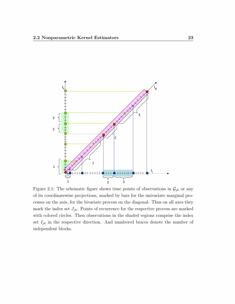
While the formal definitions look quite complicated, the main points are illustrated
in Figure 2.1. If type of index set and type of process coincide, the definition of
the index sets keeps all observations. Thus for Xj the index set Ij comprises all
observations i = 1, . . . , nj. Tough if the types do not match, some observations
might be omitted for coordinating speeds among the involved dimensions. In
summations the involved processes for the index set appear as summands - thus
for ease of notion we can leave them out in the following. Generally for a fixed
process Xj it is If ⊆ Ijk ⊆ Ij, and Ij 6= Ik and Ijk 6= Ijk′ for j 6= k 6= k′. If
βj = βk, then it is asymptotically |Ij| = |Ik|. Since in practice recurrence times
are not observable, operationalize the choice of index sets by the asymptotically
equivalent hitting times T jCj
(n) for a small set Cj ⊆ Gj. Then T jCj
(n) � T j(n)
asymptotically. The same holds for all other directions and dimensions. If G is
small for X then any of its coordinatewise projections Gfj or Gf
jk are small for
respective component directions and generally Gfj ⊆ Gj. If we choose G according
to the data, the easiest choice is according to the full dimensional X
Gf = Gf1 ⊗ . . .⊗ Gf
d . (2.12)
Selecting G is a tradeoff: Choose it big enough not to miss many observations,
choose it small enough such that still πj(1Gj) < ∞. In the sequel, there will be
the prominent case, where only pairwise properties between covariates are used
2.2 Nonparametric Kernel Estimators 23
2
1
11
2
3
2
3
3
IjkIk
Ij
Figure 2.1: The schematic figure shows time points of observations in Gjk or any
of its coordinatewise projections, marked by bars for the univariate marginal pro-
cesses on the axis, for the bivariate process on the diagonal. Thus on all axes they
mark the index set Jjk. Points of recurrence for the respective process are marked
with colored circles. Then observations in the shaded regions comprise the index
set Ijk in the respective direction. And numbered braces denote the number of
independent blocks.
24 Chapter 2. Motivation and Basic Framework
and known. For generalized smooth backfitting we work with only pairwise β–null
Harris recurrent processes, where recurrence of higher dimensional components of
or the full covariate vector is generally not the case. For this, we need to work in
pairwise adapted sets for each j = 1, . . . , d
G(j) = G(j)1 ⊗ . . .⊗ G(j)
j−1 ⊗ Gj ⊗ G(j)j+1 ⊗ . . .⊗ G(j)
d , (2.13)
where Gjk is chosen according to Xjk, and G(j)k is its coordinate projection in
direction k on Gk with k 6= j. Set Gjk = G(j)k = Gj for j = k. Here the scaling
occurs according to the highest dimensional available object where the amount of
data grows to infinity with increasing sample size. A full dimensional G with this
property is in this general setting not available.
The basic underlying estimation technique will be kernel smoothing with product
kernels. Denote
Kh (Xi − x) =1
hd
d∏j=1
K
(Xj
i − xj
h
)(2.14)
where Xi = (X1i , . . . , Xd
i ) and K is a standard kernel function. The bandwidth h
depends on the recurrence frequency of X. It is generally larger than the marginal
bandwidth choices hj for Xj. Due to possible different recurrence structures, not
only each univariate direction has in general a different bandwidth hj 6= hk for
j 6= k, but also bivariate and higher components need special bandwidth choices
different from the usual product of involved single dimensional bandwidths i.e.,
hjk 6= hjhk in general.
Assumption 2.1. 1. The univariate kernel K is symmetric about 0 and
bounded. It has compact support on Sj = [−cj, cj] with Sj ⊆ Gj. So
the Kernel can in fact depend on j, which, however, will subsequently be
suppressed in notation.
2. Furthermore K as well as K(u) ·uk has to be Lipschitz-continuous for any x
and any power k < 2p + 1 with Lipschitz constant L > 0, where p indicates
the number of partial derivatives possible for the conditional mean function
m.
2.2 Nonparametric Kernel Estimators 25
Since for general β–Harris recurrent processes no such thing as a stationary den-
sity exists, kernel density estimators converge to the corresponding more general
object, the density of the invariant measure under suitable assumptions (See The-
orem 5.1. Karlsen and Tjøstheim [2001] for exact conditions). In this sense the
unique invariant measure serves as a generalization of a stationary distribution.
Following the reasoning in the previous section, the appropriate scaling of the
usual marginal kernel density estimator πj(xj) has to be slightly modified. Paying
for the potentially nonstationary character of the marginal process Xj, the appro-
priate scaling in contrast to the usual kernel density estimate is to be adaptively
stochastic by the number of effective iid observations, thus by the number of regen-
erations (T j(n))−1
instead of the usual (n)−1. For β–Harris recurrent processes the
usual law of large numbers cannot hold anymore, but there exists a more general
analogue in the quotient limit theorem (A.11), which guarantees convergence of a
quotient of two stochastic components under quite general assumptions.
Kernel density and conditional mean estimators are defined on Gj, Gjk or Gf
bounded as
π(x) =1
T (nf )
∑i∈If
Kh(Xi − x) (2.15)
πj(xj) =
1
T j(nj)
∑i∈Ij
Khj(Xj
i − xj) (2.16)
mj(xj) =
∑i∈Ij
Khj(Xj
i − xj)Yi∑i∈Ij
Khj(Xj
i − xj)=
1
T j(nj)·∑
i∈IjKhj
(Xji − xj)Yi
πj(xj),(2.17)
where the norming function depends on the recurrence frequency of the respec-
tive processes. The above definitions can be operationalized according to (2.2)
with appropriate small sets. In the univariate case the numerator of the kernel
density estimator (2.16) can be regarded as a local time estimator. In higher
dimensions local time does not exist any more, but the numerator can still be
interpreted as an occupation time like object (see [Phillips and Park, 1998]).
Thus occupation time quantities are defined as Lj(xj) =
∑i∈Ij
Kxj ,hj(Xji ) and
26 Chapter 2. Motivation and Basic Framework
Ljk(x) =∑
i∈IjkKxjk,hjk
(Xjki ). Since it is in general
π(k)j (xj) =
∫G(j)
k
πjk(xjk)dxk 6= πj(x
j) (2.18)
πfj (xj) =
∫G(f)
k
π(x)dx−j 6= πj(xj) , (2.19)
Define π(k)j = πjk = πj for j = k. We also need to introduce
π(k)j (xj) =
1
T jk(njk)
∑i∈Ijk
Khjk(Xj
i − xj) =L
(k)j (xj)
T jk(njk)=
∫G(j)
k
πjk(xjk) dxk (2.20)
m(k)j (xj) =
∑i∈Ijk
Khjk(Xj
i − xj)Yi∑i∈Ijk
Khjk(Xj
i − xj)=
1
T jk(njk)·∑
i∈IjkKhjk
(Xji − xj)Yi
π(k)j (xj)
=∑i∈Ijk
Khjk(Xj
i − xj)Yi
L(k)j (xj)
. (2.21)
Set π(k)j = πjk = πj for j = k. Analogously derive πf
j (xj)) and mfj (x
j) from the
full dimensional process X
πfj (xj)) =
1
T (nf )
∑i∈If
Kh(Xji − xj) =
Lfj (x)
T (nf )=
∫Gf−j
πf (x) dx−j (2.22)
mfj (x
j) =
∑i∈If
Kh(Xji − xj)Yi∑
i∈IfKh(X
ji − xj)
. (2.23)
Note that the nonstationary character for the estimators in (2.20) and (2.21) is
determined by the two–dimensional type βjk. The estimators in (2.20) and (2.21)
have nonstationary type β = βf . Hence in their asymptotic behavior the first bi-
variately governed pair has a univariate rate with bivariate nonstationary character
from the data, i.e. π(k)j (xj)) − π
(k)j (xj) = bias + OP ((T jk(njk)hjk)
−1/2) + oP (h2jk)
where the bias vanishes under suitable technical assumptions with order h2jk in the
interior (See Karlsen and Tjøstheim [2001]). For (2.20) and (2.21) the statement
holds with nonstationary with rate (T (nf )h)1/2 � (nβfh)1/2 and bias of order h2.
For the rest of the paper we will suppress indices in n when appearing in recurrence
2.2 Nonparametric Kernel Estimators 27
times and hitting numbers of small sets, e.g. we write T j(n) instead T j(nj) for
ease of notation.
As in a stationary setting, since G or all G(j) are bounded, near the boundary of
the support the standard kernel estimator is poor and has considerable boundary
specific bias. This is because the kernel density estimator has no knowledge of
the boundary and may, in general, assign probability mass outside the support.
Therefore we need to slightly modify the usual kernel without harming its essential
nonnegativity. This is common practice in kernel estimation on compact sets. We
introduce the modified kernel
Kv,h(u) =Kh(u− v)∫
GjKh(w − v)dw
(2.24)
Note that for the use of modified kernels, extra attention has to be paid to the
kernel moments. It is∫Gj
Kxj ,hj(uj)duj = 1 for all xj ∈ Gj
2cjhj(2.25)
and depends on xj otherwise. Thus the corresponding Kernel constants are defined
as
κl(u) =
∫Gj
(u− v)l Khj(u− v)∫
GjKhj
(w − v) dwdv.
Easy calculations show that there are three different cases
κl(u) =
∫Gj
vlK(v) dv for u ∈ Gj,2cjhj∫Gj
vlK(v) dv + O(hjl+1) for u ∈ ∂Gj,2cjhj
\∂Gj,cjhj∫Gj
(u− v)lKhj(u− v) dv + O(hj
l+1) for u ∈ ∂Gj,cjhj
.
From now on denote by Gj,hj= Gj,2cjh the interior of interest and by ∂Gj,hj
=
∂Gj,2cjh. The modified kernels only have an influence at boundary points u ∈∂Gj,2cjh, where they differ from usual kernel constants. Analogously, kernel con-
stants κ2l =
∫Gj
(u − v)l(Khj(u, v))2 dv are defined. For the rest of this paper all
kernels are modified kernels.

28 Chapter 2. Motivation and Basic Framework
Chapter 3
Estimation
In this chapter we introduce nonparametric estimation techniques for a structural
additive model (1.1) in a β–null Harris recurrent framework. Countervailing the
standard curse of dimensionality, we impose additivity of the unknown function.
Aiming to circumvent the nonstationary curse of dimensionality, developed esti-
mation techniques are of smooth backfitting type (See Mammen et al. [1999]). The
appropriate estimation method for a given problem must be selected according to
the degree of nonstationarity in the covariate vector and according to how close
the true model is to an additive structural relationship. From standard smooth
backfitting in Section 3.2. to generalized smooth backfitting in Section 3.3 minimal
requirements on the compound covariate process can be relaxed remarkably, but
also the admissible generality in the true model decreases.
3.1 Choice of the Type of Estimation Technique
To overcome the ordinary curse of dimensionality in nonparametric statistics, the
problem is modeled additively. In a usual stationary mixing setting, there are
several kernel based techniques how to fit additive models: classical backfitting in
Buja et al. [1989] and Tibshirani and Hastie [1990], marginal integration by Linton
and Nielsen [1995] and Tjøstheim and Auestad [1994], smooth backfitting by Mam-
men et al. [1999], and the two–step local partitioned regression (LPR) approach by

30 Chapter 3. Estimation
Christopeit and Hoderlein [2006]. Though apart from backfitting type estimators,
all other procedures are based on a full–dimensional nonparametric regression pi-
lot estimate. In our setting in particular, this would require the full dimensional
process X to be Harris recurrent, which is generally too restrictive. In contrast and
with hope to countervail the nonparametric course of dimensionality, backfitting
avoids fitting a full dimensional regression estimate. The estimation procedure is
iterative where for classical backfitting in each step only one component is updated
while all others remain fixed. Therefore in fact, only one–dimensional smoothing
is applied. Asymptotic theory for classical backfitting, however, suffers from the
difficulty that the estimate is defined as the limit of the iterative backfitting al-
gorithm for which there is no explicit closed form available. Although Opsomer
and Ruppert [1997] and Opsomer [2000] could show some theoretical results under
restrictive conditions on the design densities, asymptotic inference under general
assumptions is still an open issue. Furthermore classical backfitting fails to reach
the oracle efficiency bound i.e., additive components are not estimated with the
same accuracy as if the other components were known. The bias of one additive
component depends strongly on all other directions. Even some moderate corre-
lation between covariates may cause the estimator to collapse and diverge. And
for classical backfitting to work, rather strong conditions have to be fulfilled. In
total, for general β–null Harris recurrent data, it seems more advisible to chose a
more robust technique as a starting point for estimation.
Smooth backfitting estimates (SBE) are defined as minimizers of a smoothed
least squares criterion. From this, the backfitting iteration algorithm can be de-
rived, according to which the estimates are calculated. Thus asymptotic analysis
is simplified, since the estimate is explicitly defined. In view of Mammen et al.
[2001], the SBE can also be seen as an orthogonal projection of the data vector
onto the space of additive functions. Furthermore, under weak assumptions the
SBE reaches efficiency and is furthermore robust, easy to calculate and fast (see
Mammen and Park [2005], Haag [2006] and Yu et al. [2007]). As with classical
backfitting, the SBE does not need full–dimensional estimates. But in contrast
smoothing occurs with respect to all other covariates resulting in a more robust
3.2 Standard Smooth Backfitting for Nonstationary Covariates 31
estimator. Therefore it avoids not only the ordinary stationary curse of dimension-
ality but also offers a way to countervail the nonstationary curse of dimensionality.
Since it requires only one and two–dimensional marginal processes to be pairwise
Harris recurrent, a smooth backfitting type estimator appears to be the most suit-
able choice for a recurrent setting.
3.2 Standard Smooth Backfitting for Nonsta-
tionary Covariates
Assume throughout this section that the regression model has additive form as
in (1.1). Furthermore all mentioned densities of invariant measures exist and are
finite on G or any of its subspaces. And the regression functions mj are in the
respective weighted L2πj
(Gk) spaces.
For all stationary data processes identifiability in population is achieved by∫Gj
mj(xj)πj(x
j)dxj = 0 , (3.1)
for all j = 1, . . . , d. In this standard stationary case, the smooth backfitting esti-
mators (SBE) for component functions (m0, . . . , md) are then obtained as solutions
of the following system of integral equations
mj(xj) = mj(x
j)− m0,j −∑k 6=j
∫Gk
mk(xk)
πj,k(xj, xk)
πj(xj)dxk (3.2)
m0,j =
∫Gj
mj(xj)πj(x
j)dxj∫Gj
πj(xj)dxj=
1
n
n∑i=1
Yi (3.3)
where mj is a marginal Nadaraya–Watson pilot estimator as defined in (2.17) and
πjk and πj are standard Kernel density estimators of the respective stationary
densities. The form of m0,j is determined such that (m1, . . . , md) satisfy sam-
ple analogue versions of the norming conditions in (3.1). Note that estimates
are obtained from univariate and bivariate quantities only. Contrary to ordinary
backfitting, smooth backfitting involves some additional smoothing which makes
32 Chapter 3. Estimation
it more robust. In particular, no restriction on the correlation structure of the
covariates is needed in order to obtain estimates with a well–determined asymp-
totic distribution. In the stationary case, the form of (3.2) can be additionally
motivated via a projection argument as the corresponding first order conditions
for obtaining the best additive fit to the data in a suitably π–weighted empirical
L2 norm. Smooth backfitting estimates are the best additive locally weighted least
squares approximation to the data
(mj)dj=0 = arg min
f0,...,fd
∑i∈I
∫G
(Yi − f0 − f1(x
1)− . . .− fd(xd))2
Kx,h(Xi)dx(3.4)
under the operationalized version of the norming constraint (3.1)
n∑i=1
∫Gj
mj(xj)Kxj ,h(X
ji )) dxj = 0 for j = 1, . . . , d . (3.5)
Solving (3.4) under (3.5) leads to a first order conditions of the following form∑i∈I
∫G−j
(Yi − m0 − m1(x
1)− . . .− md(xd))Kx,h(Xi)dx−j = 0 ,
for each component function mj, j = 1, . . . , d at xj ∈ Gj. With this and standard
kernel calculations, the backfitting equations (3.2) are easily derived. Detailed
calculations are shown in Mammen et al. [1999].
In a nonstationary setting, however, generally the number of data points in a
fixed bounded set is of different order for different covariates of different directions
and dimensions. However, if the full–dimensional process X is β–null Harris re-
current, we can restrict the space to Gf and its coordinatewise projections and still
have sufficiently many data points for inference. Then accordingly, all marginal
and estimated objects should be constructed from the scale of corresponding full–
dimensional objects as in (2.22) and (2.23). When replacing πj by πfj , πjk by πf
jk
and mj by mfj , we can use standard backfitting (3.2). In this setting, the projection
character remains valid as a projection on the space of functions
Hf ={
m ∈ L2π(Gf )| ∃(m1, . . . ,md) ∈ L2
πf1
(Gf1 )× . . .× L2
πfd
(Gfd ) :
m(x) = m1(x1) + · · ·+ md(x
d) for all x ∈ Gf}
3.3 Generalized Smooth Backfitting (GSBE) 33
Though it comes at a cost of neglecting a substantial amount of data not in Gf .
Furthermore, we will see, that obtained rates of convergence are slow.
3.3 Generalized Smooth Backfitting (GSBE)
If we weaken the assumption on the covariates to only pairwise pairwise β–null
Harris recurrence, the class of processes admissible for estimation is substantially
larger than the one of full β–null Harris recurrent processes, required for a fully
nonparametric regression or standard smooth backfitting. In order to construct a
general nonparametric backfitting type procedure, (3.2) shows that β–null Harris
recurrence must at least hold for all two–dimensional components. While for all
classes of γ–wise β–null Harris recurrent processes with 2 ≤ γ ≤ d a smooth
backfitting procedure can be introduced, the weakest and most general setting
of γ = 2, pairwise β–null Harris recurrence, is the most interesting setting and
deserves the main focus.
3.3.1 Generalized Smooth Backfitting for at least Pairwise
β–null Harris Recurrent Covariates
Under pairwise β–null Harris recurrence, only univariate and bivariate components
have an invariant measure, higher dimensional objects are generally not recurrent
anymore. In order to obtain smooth backfitting type estimates in this setting, we
take a corresponding suitable adaptation of the defining integral equations (3.2)
as starting point. Then the generalized smooth backfitting estimates (mj)dj=1 are
defined as solutions to
mj(xj) =
∑k 6=j
(1
d− 1
(m
(k)j (xj)− m
(k)0,j
)−∫G(j)
k
mk(xk)
πj,k(xj, xk)
π(k)j (xj)
dxk
)(3.6)
m(k)0,j =
∫Gj
m(k)j (xj)π
(k)j (xj)dxj =
1
T jk(n)
∑i∈Ijk
Yi (3.7)
where π(k)j , m
(k)j and πj,k have the same type of nonstationarity βjk and therefore
the same bandwidth and speed of convergence as defined in (2.20), (2.21) and in

34 Chapter 3. Estimation
the bivariate jk version of (2.16). For component j, the estimation relevant region
is G(j), the product of coordinatewise projections of relevant pairs, defined in (2.13)
which might be different for each j. For any k 6= j it still is m(k)j (xj)
P→ mj(xj)
under suitable additional assumptions with speed of bivariate nonstationary type
(nβjkh)−1/2. The matching norming conditions in population are∑k 6=j
∫Gj
mj(xj)π
(k)j (xj)dxj = 0 , (3.8)
for all j = 1, . . . , d. Since the estimator is constructed on the basis of pairwise
data, the asymptotic results will confirm the intuition that bivariate types of non-
stationarity govern the large sample behavior. Therefore speeds of convergence
are significantly faster then in the standard backfitting case. But in general on the
other hand, generalized smooth backfitting estimates can no longer yield the best
overall additive fit as obtained from (3.4). Since recurrence is only guaranteed for
only univariate and bivariate components, the projection character of SBE can
only prevail in a weakened pairwise sense. This is not a deficit of the estimator
but due to the difficulty of the underlying data. Therefore the underlying model
must truly at least be additive in pairs of components, i.e. of the form
Yi =∑j 6=k
mjk(Xjki ) + εi , (3.9)
for SBE to still yield a sensible approximation to the truth. Then SBE produces the
best pairwise additive approximation to (3.9) for each component j by projecting
orthogonally via
[µk|jmjk](xj) =
∫G(j)
k
mjk(xjk)
πjk(xjk)
π(k)j (xj)
dxk , (3.10)
for j 6= k on
Hjk =
{m ∈ L2
πjk(Gjk)| ∃(mj, mk) ∈ L2
π(k)j
(G(k)j )× L2
π(j)k
(G(j)k ) :
m(x) = mj(xj) + mk(x
k) for all x ∈ Gjk
}(3.11)
3.3 Generalized Smooth Backfitting (GSBE) 35
for each k, where in the case k = j it is Hjj = Hj = L2πj
(Gj), and adding up the
results. The corresponding system of population equations to this approximation
are for j = 1, . . . , d
E(Yi|Xji ) = mj(X
ji ) +
∑k 6=j
E(mjk(Xjki )|Xj
i ) . (3.12)
Therefore, since a best fit is merely achieved in a pairwise sense (3.10), in general,
correlation structures beyond pairwise correlation cannot be captured within the
estimation procedure and must be regulated through additional assumptions. If
all regressors are stationary, (3.6) reduces to (3.2) and the norming constraint (3.8)
to (3.1). Thus standard smooth backfitting equations are a subcase of generalized
smooth backfitting.
We obtain the backfitting estimates as solution to (3.6) via iteration. Start at
an arbitrary initial guess m[0]j , e.g. the Nadaraya–Watson estimator m
[0]j = mj.
Then denote the rth step iterate of the jth component with m[r]j . Hence iterate
according to
m[r]j (xj) =
1
d− 1
∑k 6=j
(m
(k)j (xj)− m
(k)0,j
)−∑k<j
∫G(j)
k
m[r]k (xk)
πj,k(xj, xk)
π(k)j (xj)
dxk −
−∑k>j
∫G(j)
k
m[r−1]k (xk)
πj,k(xj, xk)
π(k)j (xj)
dxk (3.13)
until a convergence criterion is fulfilled. In the simulation study we employ a
standard quotient condition for termination.
Note that∑
k 6=j m(k)0,j is only different from zero, when the norming condition
(3.8) is violated. If we set directly
m0 =d∑
j=1
1
d− 1
∑k 6=j
1
T jk(n)
∑i∈Ijk
Yi , (3.14)
an appropriate sample mean type expression, the centering term m(k)0,j can be omit-
ted from the algorithm.
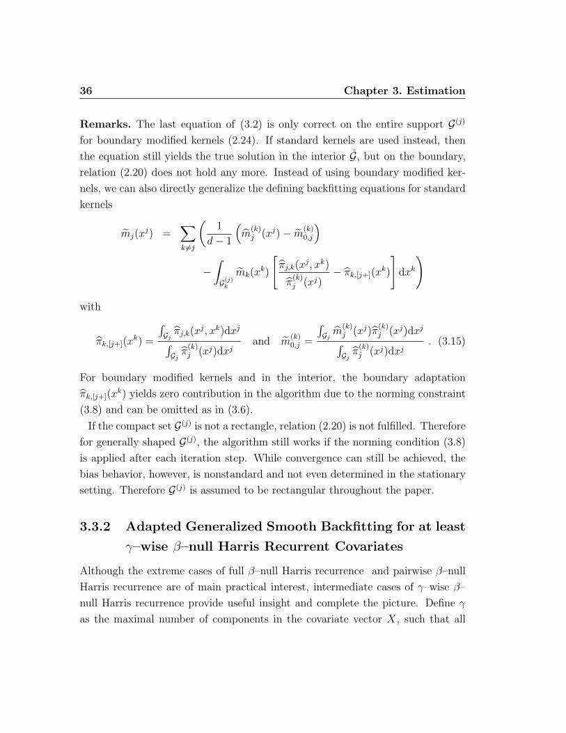
36 Chapter 3. Estimation
Remarks. The last equation of (3.2) is only correct on the entire support G(j)
for boundary modified kernels (2.24). If standard kernels are used instead, then
the equation still yields the true solution in the interior G, but on the boundary,
relation (2.20) does not hold any more. Instead of using boundary modified ker-
nels, we can also directly generalize the defining backfitting equations for standard
kernels
mj(xj) =
∑k 6=j
(1
d− 1
(m
(k)j (xj)− m
(k)0,j
)−∫G(j)
k
mk(xk)
[πj,k(x
j, xk)
π(k)j (xj)
− πk,[j+](xk)
]dxk
)
with
πk,[j+](xk) =
∫Gj
πj,k(xj, xk)dxj∫
Gjπ
(k)j (xj)dxj
and m(k)0,j =
∫Gj
m(k)j (xj)π
(k)j (xj)dxj∫
Gjπ
(k)j (xj)dxj
. (3.15)
For boundary modified kernels and in the interior, the boundary adaptation
πk,[j+](xk) yields zero contribution in the algorithm due to the norming constraint
(3.8) and can be omitted as in (3.6).
If the compact set G(j) is not a rectangle, relation (2.20) is not fulfilled. Therefore
for generally shaped G(j), the algorithm still works if the norming condition (3.8)
is applied after each iteration step. While convergence can still be achieved, the
bias behavior, however, is nonstandard and not even determined in the stationary
setting. Therefore G(j) is assumed to be rectangular throughout the paper.
3.3.2 Adapted Generalized Smooth Backfitting for at least
γ–wise β–null Harris Recurrent Covariates
Although the extreme cases of full β–null Harris recurrence and pairwise β–null
Harris recurrence are of main practical interest, intermediate cases of γ–wise β–
null Harris recurrence provide useful insight and complete the picture. Define γ
as the maximal number of components in the covariate vector X, such that all
3.3 Generalized Smooth Backfitting (GSBE) 37
possible permutations of γ dimensional compound component processes are still
β–null Harris recurrent. Assume we have a γ–wise β–null Harris recurrent process.
If the process is fully β–null Harris recurrent, we have γ = d, if it is only pairwise
β–null Harris recurrent, it is γ = 2. Intermediate cases have 2 < γ < d. In order
to treat all these cases simultaneously, we need to introduce some notation. Set
κ as multiindex in Rd with κl ∈ {0, 1} for all l = 1, . . . , d and |κ| =∑d
l=1 κl = γ,
indicating the dimensions involved by 1 and dimensions left out by 0, where there
always are γ dimensions involved. Furthermore put
λ(κ) = {l|κl = 1, l = 1, . . . , d} , (3.16)
and λj(κ) = {l|κj = 1 and κl = 1, l ∈ {1, . . . , d} \ {j}} and λjk =
{l|κjk = 1 and κl = 1, l ∈ {1, . . . , d} \ {j, k}}. When projecting a function
mk ∈ L2πk
(Gk) on L2πj
(Gj), for nonstationary data with γ–wise β–null Harris
recurrence, an orthogonal projection in the appropriate conditional expectation
sense looks like [µ(λjk)
k|j mk](xj) =
∫mk(x
k)π
(λjk)
jk (xjk)
π(λj)
j (xj)dxk. Though for γ > 2 there
are(
dγ−2
)different versions to construct such a projection since then λjk 6= ∅ for
j 6= k. Therefore for each component function generalized smooth backfitting
yields(
dγ−2
)estimates under γ–wise β–null Harris recurrence indexed by λjk
m(λjk)j (xj) =
∑k 6=j
(1
d− 1
(m
(kλjk)j (xj)− m
(kλjk)0,j
)(3.17)
−∫G
(jλjk)
k
m(λjk)
k (xk)π
(λjk)
j,k (xj, xk)
π(kλjk)j (xj)
dxk
)
m(kλjk)0,j =
∫G
(λjk)
j
m(kλjk)j (xj)π
(k)j (xj)dxj =
1
T jkλjk(n)
∑i∈Ijkλjk
Yi .
To obtain a single final estimate take the pointwise arithmetic mean or median of
(m(λjk)j )λjk for each component j. The matching norming conditions in population
are ∑k 6=j
∫Gj
mj(xj)π
(kλjk)j (xj)dxj = 0 , (3.18)
38 Chapter 3. Estimation
for all j = 1, . . . , d. If all regressors are stationary, (3.17) reduces to (3.2) and the
norming constraint (3.18) to (3.1). Thus ordinary backfitting is also a subcase of
generalized backfitting under γ–wise β–null Harris recurrence .
Under γ–wise β–null Harris recurrence , the data allows to control correlation
structures up to order γ within the SBE procedure as defined in (3.17). Thus
if the underlying covariates show a “nicer” nonstationary behavior than in the
pairwise β–null Harris recurrent case, we need less extra assumptions to regulate
higher order correlation structures. Furthermore the underlying model can be
more general than (3.9). In fact, (3.17) yields a sensible additive approximation
for γ–wise additive functions. In population for j = 1, . . . , d this corresponds to
E(Yi|Xji ) = mj(X
ji ) +
∑k 6=j
E(mjkλjk(X
jkλjk
i )|Xji ) . (3.19)
Chapter 4
Asymptotic Results
In this chapter the main asymptotic results are stated. The focus is on the prac-
tically most interesting extreme cases: smooth backfitting for a full–dimensional
β–null Harris recurrent vector of covariates and generalized smooth backfitting for
at least pairwise β–null Harris recurrent regressors. In a nonstationary setting,
generally the difficulty of the problem with different data for different directions
and dimensions will affect the result through the type of β to which the backfitting
estimation technique is scaled, while keeping the univariate structure in rates and
variances as in stationary smooth backfitting. From the construction of generalized
smooth backfitting, it is clear that we cannot do better in terms of data and thus
in type of nonstationarity than in the worst bivariate case. For standard smooth
backfitting even the generally much smaller and thus less favorable full dimensional
type of nonstationarity β governs procedure and results. Therefore, although rates
and variances have the form as for one–dimensional marginal smoothers, generally
we cannot expect full oracle behavior of the estimates as in the stationary case.
For a true additive model, the asymptotic expansion of GSBE in Section 4.2 is
obtained under the weakest assumptions and yields the most efficient results in an
oracle sense even if covariates are γ–wise β–null Harris recurrent with 2 < γ ≤ d.
Asymptotic results for the generalized smooth backfitting adapted to γ–wise β–
null Harris recurrence are mentioned for completeness in the Section Extensions.
Here we study how more information about the type of underlying data, can im-

40 Chapter 4. Asymptotic Results
prove efficiency of the estimation procedure. Of practical interest is in particular
a tailored procedure for covariates with known stationary and nonstationary com-
ponents which has nice small sample properties. For all proofs we refer to the
Appendix.
4.1 Standard Smooth Backfitting for Nonsta-
tionary Covariates
In this subsection we present the base case scenario when the full process is β–
null Harris recurrent. In this class of processes we can obtain asymptotic results
without further restrictions on the dependence structure among the covariates or
for the estimated functions in a nonstationary framework. Furthermore even if
the underlying model is not additive, it yields the best additive fit. However,
when requiring β–null Harris recurrence for full X, only the standard curse of
dimensionality is reduced, while the nonstationary curse of dimensionality remains
the same as for standard regression with non–additive m.
Assumption 4.1. Let X be an irreducible aperiodic Markov chain, which is β–
Harris recurrent of type β. The invariant measure π has a Radon–Nikodym deriva-
tive with respect to Lebesgue measure which is finite on G = Gf . The invariant
density π is bounded and has continuous second partial derivatives. Furthermore
π is bounded away from zero.
Note that πf (G) < ∞ is obtained if G is small for X. Therefore in general, the
choice of G is difficult, since size and form of G is determined by the process X.
Though if X is Feller, any compact G is small.
Under Assumption 4.1, we can construct all relevant objects according to the full
dimensional process as in (2.11),(2.12), (2.22), and (2.23). Thus in this setting,
when replacing πj by πfj , πjk by πf
jk and mj by mfj , standard smooth backfitting
algorithm from (3.2) does not need any modification to directly be a sequence
of iterated projections. The generalized smooth backfitting reduces to standard
smooth backfitting. With this procedure, however, we can only manage to reduce
4.1 Standard Smooth Backfitting for Nonstationary Covariates 41
the standard stationary type curse of dimensionality, whereas the nonparamet-
ric curse of dimensionality remains untouched. This is intuitively clear, when we
restrict all marginal univariate and bivariate processes to the full dimensional com-
mon set of data Gf and all estimators have the same but full dimensional type of
nonstationarity β. Therefore the speed of convergence for the smooth backfitting
estimator is governed by the occupation time Lfxj ,h
for the full dimensional process.
Other than for stationary data, this implies that through the standardization with
X we might lose a substantial amount of data for univariate and bivariate compo-
nents. Therefore the procedure cannot be oracle as soon as one of the covariates
is nonstationary.
For identification of the estimation problem (3.2) the dependence structure be-
tween regressors X and the residual ε must be restricted. In our general poten-
tially nonstationary setting usual conditional independence assumptions only have
a meaning with respect to an appropriate invariant measure. Furthermore to have
a controllable asymptotic behavior of estimators, the compound chain (X, ε) on
G × G0 must satisfy certain assumptions.
Assumption 4.2.
1. The compound chain (X, ε) is a φ–irreducible β–null Harris recurrent Markov
chain with transition probability operator P and density πfε of the invariant
measure, where πεf (x) =
∫G0
πfε(x, ε) dε > 0 for all x ∈ G and πεf (G) < ∞.
2. µε|f (x) = 0 and σ2ε|f (x) < ∞ for all x ∈ G, where both quantities are de-
fined with respect to invariant measures µε|f (x) =∫
επfε(x,ε)
πεf (x)
dε and σ2ε|f (x) =∫
ε2 πfε(x,ε)
πεf (x)
dε.
3. The marginal transition probability operator Px of X is independent of any
initial distribution. And for sets Ah ∈ B∞(Rd+1) with limh→0 Ah = ∅ it is for
the compound transition probability lim supξ→x limh→0
∫P ((ξ, ε), Ah) |ε| dε =
0 for all x ∈ G.
4. ε has bounded support G0 and the set G ⊗ G0 is small for (X, ε), where G is
defined as inth(G) = G.

42 Chapter 4. Asymptotic Results
5. The second partial derivatives of the function m exist and are Lipschitz con-
tinuous.
Finiteness of the measure πεf on G in Assumption 4.2.1 implies that the asymp-
totic behavior of the compound process (X, ε) is dominated by the β–null structure
of the X component (see Karlsen et al. [2007], Lemma 6.1.). It is πf (x) = c πεf (x)
with c constant. Thus πεf also inherits differentiability properties of πf from As-
sumption 4.1. In Assumption 4.2.2 the identifying conditional independence cri-
terion is specified. All subsequent assumptions are needed to control the asymp-
totic behavior of the compound chain. Assumption 4.2.3 states a local uniform
continuity assumption on the transition probability operator P , which allows to
control and simplify the variance part in the smoothing as shown in Lemma 5.1. in
Karlsen and Tjøstheim [2001]. All these assumptions 4.2.1 - 4.2.3 can be regarded
as somehow natural and/or minor technical restrictions. In contrast, however,
Assumptions 4.2.4 might appear artificial and technical. Smallness, however, is
crucial for controlling stochastic terms of the form fx(Xi, εi) = Kh,x(Xi)εi for
x ∈ Gf in the estimators. Under Assumption 2.1 on the smoothness of the kernel,
f is in particular bounded and therefore small and thus special (see Proposition
5.13. in Nummelin [1984]). This implies
supy∈G×G0
Ey
τ∑i=1
Kh,x(Xi)εi < ∞ for all x ∈ G . (4.1)
With Assumption 3.5 also fx(Xi) = Kh,x(Xi)m(Xi) is special for each x ∈ G and
fulfills (4.1). Note, that weakening the condition towards unbounded support and
subexponential tails is not admissible, as trimming techniques in the proofs would
fail. Compare that in Karlsen et al. [2007] equivalent pointwise conditions were
needed to obtain central limit theorems in such a general framework.
Remark 4.1. Note that Assumptions 4.2 only require a conditional independence
condition with respect to invariant measures. Thus short term dependence between
residual and covariates is admissible as long as it vanishes asymptotically. This is
a much weaker requirement than full independence (see Examples 6.1. and 6.2. in
4.1 Standard Smooth Backfitting for Nonstationary Covariates 43
Karlsen et al. [2007] for examples of asymptotically but not fully independent resid-
uals). Thus in Econometric terms, we can identify the model under endogeneity.
The problem remains well–posed as long as dependence vanishes asymptotically.
This is opposed to results in the iid case, where any form of endogeneity directly
leads to ill–posedness of the problem requiring regularization methods and thus
a yielding severely deteriorated small sample behavior (compare Carrasco et al.
[2003]).
If ε is ergodic and fully independent of X, we can omit the boundedness and
smallness assumption. It is of particular interest to have a closer look at models
with ε stationary, since these cases can be regarded as an additive cointegration
type model. The more regularity ε offers, the more familiar turn the conditions
to the stationary case. Under full independence between ε and X, the catalogue
of Assumptions 4.2 simplifies to moment conditions for ε being α–mixing and the
smallness condition can be avoided.
Assumption 4.2*
1. X and ε are independent β–null Harris recurrent Markov chains
2. ε is ergodic strongly α–mixing with mixing rate satisfying∑
l l[2/k]∨1αl <
∞, µ(ε) =∫
επε(ε) dε = 0 and∫
ε4(k+1)πε(ε) dε < ∞ with k ≥ 1.
3. For sets Ah ∈ B∞(Rd) with limh→0 Ah = ∅ the transition probability of X
fulfills lim supξ→x limh→0 P ((ξ), Ah) = 0 for all x ∈ G.
4. The second partial derivatives of the function m exist and are Lipschitz con-
tinuous.
Remark 4.2. If all moments on the residual process are finite, it is sufficient if
there exists a δ > 0 such that∑
l α1−δl < ∞ for the mixing coefficients.
Note that in general we need the existence of at least the 8th moment. In the
error term. Though if ε is strictly stationary linear, the moment conditions in
Assumption 4.2* can be relaxed.

44 Chapter 4. Asymptotic Results
Remark 4.3. If ε is strictly stationary linear, it can be written as εi =∑∞
k=0 akei−k
with coefficients∑
k |ak| < ∞ and e strictly stationary with Ee0 = 0, Ee40 < ∞, and
φ–mixing1 with∑
l φ1/2l < ∞. These conditions can replace Assumption 4.2*.2.
Note that these conditions are trivially fulfilled for ei iid.
We define the Nadaraya-Watson smooth backfitting estimators
mj(xj), j = 1, . . . , d as the iterative solution of the set of equations (3.6)
and the normalization (3.8). With m0 = 1T (n)
∑i∈I Yi centering can be omitted in
the algorithm. Asymptotic properties of the estimators are stated in the following
theorem.
Theorem 4.1. Let the model be additive as in (1.1) and Assumptions 1-3 hold.
The bandwidth sequence must satisfy n−(β
4+ε)
f � h � n−(β
5+ε)
f with ε > 0 arbitrarily
small. Then the algorithm (3.13) converges with geometric rate and the smooth
backfitting estimators mj(xj), j = 1, . . . , d have the following asymptotic expansion√
Lfj (x
j)h(mj(x
j)−mj(xj)−Bj(x
j)) D−−→ N
(0, σ2
j (xj)
κ20(x
j)
κ0(xj)2
)(4.2)
with variance
σ2j (x
j) =
∫ε2
πfjε(x
j, ε)
πfεj (xj)
dε
and bias consisting of two major parts Bj(xj) = BA
j (xj) + BBj (xj). With A the
backfitting operator matrix as in (A.15), the bias parts BAj (xj) and BB
j (xj) have
the form
BBj (xj) = h
κ1(xj)
κ0(xj)m′
j(xj)− bj + h2κ2(x
j)
κ0(xj)
((I − A)−1B
)(j)
(xj) (4.3)
BAj (xj) = µf
(jε)
(Kxj ,h(X)⊗ T fε(n)
Lf (xj)
). (4.4)
Under the stated choice of bandwidth the asymptotic bias BAj vanishes. For the
deterministic bias BBj it is bj = oP (h2) in G and B(x) = (b1(x
1), . . . , bd(xd))T with
1See Hall and Heyde [1980], page 277 for an exact definition of φ–mixing
4.1 Standard Smooth Backfitting for Nonstationary Covariates 45
component functions bj for j ∈ {1, . . . , d} defined by
bj(xj) =
κ2(xj)
κ0(xj)
(1
2m′′
j (xj) +
m′j(x
j)
π(x)
∂π(x)
∂xj
)Remarks. 1. The vector of component estimates (mA
1 (x1), . . . , mAd (xd))
converges even jointly to the multivariate normal distribution
N (0, diag(σ1(x1), . . . , σd(x
d))) with 0 ∈ Rd. Covariances vanish
asymptotically.
2. The unusual restriction from above on the bandwidth is due to the non-
stationarity in the data. With this and Assumption 3.3. about the sec-
ond derivatives, the stochastic bias BAj vanishes (See Karlsen and Tjøstheim
[2001] Theorem 5.3. and Karlsen et al. [2007] Theorem 5.5.). Furthermore
under the upper bound on the bandwidth it is√
Lfj (x
j)h BBj (xj) = oP (1)
for all xj, causing the bias to disappear (See Karlsen and Tjøstheim [2001],
proof of Theorem 3.5). Thus the speed of convergence in Theorem 4.1 can
be arbitrarily close to but never attains n−25β under the stated choice of
bandwidth.
3. The result holds more generally for a model with transformed error term gε(ε)
when replacing ε in Assumption 4.2 by gε(ε) and gε is bounded and L1(R+).
Then Theorem 4.1 holds with asymptotic bias as BAj (xj) = µ(jε)(Kxj ,h(X)⊗
gε(ε))T fε(n)
Lf (xj)and variance σ2
j (xj) =
∫gε(ε)
2 πjε(xj ,ε)
πεj (xj)
dε. With considerations in
Karlsen et al. [2007], Section 6.4., and Mammen and Nielsen [2003], results
can be even further extended to models with heteroscedastic error terms.
4. In this setting, the underlying model does not have to be additive. Even if it
is not, (mj)dj=0 are optimal in the sense of an additive projection on L2
π the
best additive fit.
5. In the special case of one nonstationary regressor and all other regressors
stationary, the nonstationary rate dominates in all component functions.
46 Chapter 4. Asymptotic Results
The marginal variance σ2j (x
j) of the jth additive component is exactly the vari-
ance of the one–dimensional smoother. It can also be regarded as the projection
of σ2ε , the variance of the iid-parts in the ε split chain, onto Xj in the following
sense: E [σ2ε |Xj = xj].
As in the stationary case, the deterministic bias BBj of the Nadaraya–Watson
type smooth backfitting estimator consists of three main parts. In addition to
the marginal Nadaraya–Watson bias hκ1(xj)κ0(xj)
m′j(x
j) + 12h2 κ2(xj)
κ0(xj)m′′
j (xj) there is the
constant shift bj from a difference in population centering as in (3.8) and centering
with the population counterpart. Furthermore there exists a design density de-
pendent part((I − A)−1B
)(j)
(xj). The term bj converges to zero asymptotically
since it holds that∫∫mj(x
j)πj(u)Kh,xj(u) du dxj
=
∫uj∈∂Gj
hC1
∫mj(x
j)πj(xj)(Kh(x
j, uj)−Kh(xj − uj)) dxj duj + O(h2) = O(h) .
and the second term is of order O(h2) because κ1(xj) is zero at interior points
xj. To stress the projection character of bj(xj) = ((I − A)−1B)(j)(x
j) with ι =
(1, . . . , 1) ∈ R1×d it is:
(b0, b1(x1), . . . , bd(x
d)) = arg minb1,...,bd
∫(ιB(x)− b0 − b1(x
1)− · · · − bd(xd))2π(x) dx .
The explicit form of the projection part in the deterministic bias BBj (xj) is
((I − A)B
)(j)
(xj) =1
2m′′
j (xj) +
m′j(x
j)
πj(xj)
∂πj(xj)
∂xj
+∑k 6=j
∫Gk
(1
2m′′(xk) +
m′j(x
j)
πjk(xjk)
∂πjk(xjk)
∂xj
)πjk(x
jk)
πj(xj)dxk .
In total, the deterministic bias BBj is of order o(h2) in the interior of the estimated
compact set as in the stationary case. In the stated form above this is not obvious
at first glance. But by symmetry of the kernel, κ1(xj) is zero for xj ∈ Gj,h.
Therefore all O(h) terms vanish in the interior.
4.1 Standard Smooth Backfitting for Nonstationary Covariates 47
It can be shown that h2bj,n = O(1). This is a consequence of the centering
constraint in the algorithm, which causes lower order terms to be zero. This term
is constant over xj and does therefore only affect the level and not the shape
of the estimator. It originates from the fact that the empirical version of the
normalization (3.8) used in the algorithm and the actual theoretical normalization
(3.8) are different in finite samples and only asymptotically equivalent.
The stochastic bias BAj vanishes with oP (h2) under the stated bandwidth as-
sumptions (See Karlsen et al. [2007]). With stronger independence assumptions
on the error term as below, it can be omitted.
If we enforce the independence assumption between Xj and ε, from conditional
independence to full independence, we can avoid the artificial boundedness and
small set assumption and have more familiar moment conditions. If in addition ε
is assumed to be stationary, also the variance is no longer only a second moment
with respect to an invariant measure but with respect to the stationary density of
ε, hence a “real” variance.
Theorem 4.2. Let the same set of assumptions as in Theorem 4.1 hold, but replace
Assumptions 4.2 by Assumptions 4.2*. Choose the bandwidth as n−(β
4+ε)
f � h �
n−(β
5+ε)
f with ε > 0 arbitrarily small. Then the algorithm (3.13) converges and we
get the following asymptotic expansion for the smooth backfitting estimates (mj)dj=1√
Lfj (x
j)h(mj(x
j)−mj(xj)−BB
j (xj)) D−−→ N
(0, σ2
j (xj)
κ20(x
j)
κ0(xj)2
)(4.5)
with deterministic bias as in 4.3 and variance
σ2j (x
j) = σ2j =
∫ε2πε(ε) dε ,
where πε is the stationary density of ε.
Here the stochastic bias BAj as in (4.4) is zero under Assumptions 4.2*. The
same result also holds under milder moment conditions as in Assumption 4.2* as
specified in Remark 4.3.
48 Chapter 4. Asymptotic Results
4.2 GSBE
In the subsection before, we managed to reduce the stationary curse of dimensional-
ity via standard smooth backfitting for the additive model while the nonstationary
curse remained untouched. Therefore the resulting speed of convergence is quite
slow governed by the full dimensional β. The final version of the generalized back-
fitting estimation procedure (3.6), however, contains just one–and two dimensional
marginal components. Thus under some mild additional assumptions, we cannot
only increase the speed of convergence to be of two–dimensional nonstationary β
type, but even more importantly increase the treatable class of processes substan-
tially from full β–null Harris recurrent to just pairwise β–null Harris recurrent
processes. If the underlying model is additive, we derive the asymptotic results.
Naturally, all assumptions are restrictions on pairwise components only.
Assumption 4.3. Let X be an irreducible aperiodic Markov chain. All univariate
possible pairs of bivariate marginal processes Xjk are β–null Harris recurrent with
parameter βjk. Their respective invariant measure has a Radon–Nikodym deriva-
tive πjk with respect to Lebesgue measure. Any bivariate invariant density πjk is
bounded and has continuous second partial derivatives on Gjk. Furthermore any
πjk is bounded away from zero.
Finiteness of bivariate and univariate invariant measures is achieved, if Gjk and
Gj are small. Then for any component j we choose the space composed of pairwise
coordinate projections G(j) as defined in (3.11) as space of estimation.
Please note that theses assumptions do not restrict the pairwise correlation
structure of the covariates. Pairwise β–Harris recurrence does not rule out or re-
strain dependence of regressors. Furthermore, pairwise β–Harris recurrence is truly
weaker than full dimensional β–Harris recurrence. For example, a d–dimensional
vector of random walks is pairwise β–Harris recurrent independent of the correla-
tion structure between the covariates - while it is not fully β–Harris recurrent for
d ≥ 2 unless covariates are substantially correlated.
Identification and asymptotic expansion of generalized smooth backfitting esti-
mates (3.6) can be obtained by the following assumptions.
4.2 GSBE 49
Assumption 4.4. For any bivariate marginal process Xjk with j, k = 1, . . . , d we
assume:
1. The compound chain (Xjk, ε) is a φ–irreducible Harris recurrent Markov
chain with transition probability operator Pjkε and density πjkε of the invari-
ant measure, where πεjk(x
jk) =∫G0
πjk,ε(xjk, ε) dε > 0 for all xjk ∈ Gjk and
πεjk(Gjk) < ∞
2. µε|jk(xjk) = 0 and σ2
ε|jk(xjk) < ∞ for all xjk ∈ Gjk where both quantities are
defined with respect to invariant measures µε|jk(xjk) =
∫ε
πjkε(xjk,ε)
πεjk(xjk)
dε and
σ2ε|jk(x
jk) =∫
ε2 πjkε(xjk,ε)
πεjk(xjk)
dε.
3. The marginal transition function Pjk is independent of any initial distribu-
tion. And for sets Ah ∈ B∞(R3) with limh→0 Ah = ∅ it is for the compound
transition probability: limh→0 lim supξ→xjk
∫P ((ξ, ε), Ah) |ε| dε = 0 for all
xjk ∈ Gjk.
4. ε has bounded support G0 and the set Gjk ⊗ G0 is small for (Xjk, ε), where
inth(Gjk
)= Gjk.
5. The second partial derivatives of the function m exist and are Lipschitz con-
tinuous.
The same remarks as for Assumption 4.2 apply. In particular Remark 4.1 about
well–posedness of the problem under short–run endogeneity also applies. Further-
more it is also in this general setting of particular interest to have a closer look at
models with ε stationary, since these cases can be regarded as an additive cointe-
gration type model. If ε is α–mixing and independent of each pair of covariates,
identification requirements simplify to moment conditions.
Assumption 4.4*
For every bivariate marginal process Xjk we have:
1. Xjk and ε are independent Harris recurrent Markov chains
50 Chapter 4. Asymptotic Results
2. ε is ergodic strongly α–mixing with mixing rate satisfying∑
l l[2/k]∨1αl <
∞, µ(ε) =∫
επε(ε) dε = 0 and∫
ε4(k+1)πε(ε) dε < ∞ with k ≥ 1 .
3. For sets Ah ∈ B∞(R2) with limh→0 Ah = ∅ the transition probability of Xjk
fulfills lim supξ→x limh→0 P ((ξ), Ah) = 0 for all x ∈ Gjk.
4. The second partial derivatives of the function m exist and are Lipschitz con-
tinuous.
If moments of all order exist Remark 4.2 applies also here. Note that in general
we need the existence of at least the 8th moment in the error term. Though if
ε is strictly stationary linear, the moment conditions in Assumption 4.4* can be
relaxed.
Remark 4.4. If ε is strictly stationary linear, it can be written as εi =∑∞
k=0 akei−k
with coefficients∑
k |ak| < ∞ and e strictly stationary with Ee0 = 0, Ee40 < ∞, and
φ–mixing2 with∑
l φ1/2l < ∞. These conditions can replace Assumption 4.4*.2.
These conditions are trivially fulfilled for ei iid.
Though in contrast to the full dimensional β–null Harris recurrent case, we need
an additional assumption for controlling the bias term in order to reach consistency
of the estimation procedure.
Assumption 4.5. Assume that for all Xjli there exists a Xjk
i such that mk(Xki ) =
ml(Xli) for i ∈ Ijk and j 6= k 6= l.
This implies that on the domain G(j) all component functions must have the same
range. Implicitly, therefore the size of G(j)k can be restricted to fit Assumption 4.5.
If pairs of covariates are correlated and are close in type of nonstationarity the
requirement is mild. If the model entirely consists of trigonometric component
functions as in the simulation study, Assumption 4.5 is trivially fulfilled. Alter-
natively to Assumption 4.5 in some case as e.g. it might advisible to impose a
parametric restriction on the component functions outside small sets. See Figure
2See Hall and Heyde [1980], page 277 for an exact definition of φ–mixing
4.2 GSBE 51
A.1 in the Appendix for a discussion and Subsection A.2.3 for a discussion with
technical details.
For each component function mj it will be the worst case bivariate nonstation-
ary type jk0 dominating the asymptotic behavior. Therefore set βj+ = βjk0 =
mink 6=j βjk, nj+ = njk0 as defined in Section 2.2 and the respective bandwidth hj+
for all j = 1, . . . , d. Then we get the following closed form expansion.
Theorem 4.3. Let the model be additive as in (1.1) fulfilling the centering con-
dition (3.8) and let Assumptions 2.1, 4.3, 4.4, and 4.5 hold. The bandwidth
sequence must satisfy n−(βj+
4+ε)
j+ � hj+ � n−(βj+
5+ε)
j+ for ε > 0 arbitrarily small.
Then the algorithm (3.13) converges with geometric rate and for the estimators
mj(xj), j = 1, . . . , d we find√
L(k0)j (xj)hj+
(mj(x
j)−mj(xj)−Bj(x
j)) D−−→ N
(0, σ2
j+(xj)κ2
0(xj)
κ0(xj)2
)(4.6)
with variance
σ2j+(xj) =
∫ε2
πk0jε (xj, ε)
π(k0)j (xj)
dε
and bias consisting of two major parts Bj(xj) = BA
j (xj) + BBj (xj) with
BBj (xj) = hj+
κ1(xj)
κ0(xj)m′
j(xj) +
1
2h2
j+
κ2(xj)
κ0(xj)m′′
j (xj) +
((I − A)−1B
)(j)
(xj)− bj,n(4.7)
BAj (xj) = µ((j+)ε)(Kxj ,h(X)⊗ idε)
T (j+)ε(n)
Lj+(xj)(4.8)
Under the stated choice of bandwidth the asymptotic bias BAj vanishes. For the
deterministic bias BBj , A is the backfitting operator matrix as in (A.15) and B(x) =
(b1(x1), . . . , bd(x
d))T and component functions bj for j ∈ {1, . . . , d} defined by
bj(xj) = h2
j+
[(bj +
∑k 6=j
∫G(j)
k
bjk(xk) +
πjk(xk)
π(k)j
dxk
)](xj) .
The exact form of these bias components is given right below. Most importantly
it is bj = O(h2
j+
). Furthermore the centering constant bj,n is given by bj,n =
52 Chapter 4. Asymptotic Results
µ(j)
(Φjmj
)where the centering operator is defined in (A.15), and it is h2
j+bj,n =
O(1).
The exact form of the bias is
bj(xj) =
κ2(xj)
κ0(xj)
(m′
j(xj)
π(k)j (xj)
π(k)j
′(xj)
)
bjk(xjk) =
κ2(xj)
κ0(xj)
(m′
k(xk)
πjk(xjk)
∂πjk(xjk)
∂xk
)Remark 4.5. 1. Here the underlying model must at least be pairwise additive
as in (3.9).
2. The stated result also holds with a slight modification in some constants
under some milder assumption than Assumption 6. If we assume instead
that∫
Ajkml(x
l)πl(xl) dxl < ∞ for j 6= k 6= l where the area of integration
Ajk is defined by the correlation between components (Xjk) and X l. Details
are contained in the proof in the appendix.
3. The vector of component estimates (mA1 (x1), . . . , mA
d (xd)) converges jointly
to the multivariate normal distribution N (0, diag(σ1+(x1), . . . , σd+(xd)))
with 0 ∈ Rd. Covariances vanish asymptotically.
4. The result also holds more generally for a model with transformed error term
gε(ε) when replacing ε in Assumption 5.3 by gε(ε). Then Theorem 4.3 holds
with modified asymptotic bias BAj (xj) and variance σj(x
j) as described in
remark 3 after Theorem 4.1.
5. In the special case of one nonstationary regressor and all other regressors sta-
tionary, the nonstationary rate dominates in all component functions. Since
such a process can be easily shown to also be fully β–null Harris recurrent,
we can proceed with the easier algorithm as in the subsection before and
reach the same result.
The marginal variance σ2j+(xj) of the jth additive component is in form exactly
the variance of the one–dimensional smoother. Though the rate of convergence

4.2 GSBE 53
is of univariate character in its form but governed by the worst case bivariate
nonstationarity type βj+ for each component function.
As in the stationary case, the deterministic bias BBj of the Nadaraya–Watson
smooth backfitting estimator consists of three main parts. In addition to the
marginal Nadaraya–Watson bias hj+κ1(xj)κ0(xj)
m′j(x
j) + 12h2
j+κ2(xj)κ0(xj)
m′′j (x
j) there is the
constant shift bj,n from norming and centering and the design density dependent
part((I − A)−1B
)(j)
(xj). We pay a price for nonstationarity as the entire deter-
ministic bias BBj is of order o(h2
j+) in the interior of Gj instead of the significantly
faster o(h2j) in a stationary setting. Furthermore as generally no full dimensional π
exists as in the previous subsection, the design dependent deterministic bias part
resembles its counterpart in the full–dimensional β–null Harris recurrent case in
form, but lacks its projection interpretation. Furthermore, it can be shown that
h2j+bj,n = O(1). As before, this is a consequence of the centering constraint in the
algorithm, which causes lower order terms to be zero. This term is constant over
xj and does therefore only affect the level and not the shape of the estimator. It
originates from the fact that the empirical version of the normalization used in
the algorithm and the actual theoretical normalization (3.8) are different in finite
samples and only asymptotically equivalent.
The stochastic bias BAj vanishes with oP (h2
j+) under the stated bandwidth as-
sumptions (See Karlsen et al. [2007]). With stronger independence assumptions
on the error term as below, it can be omitted. If we enforce the independence as-
sumption between Xj and ε, from conditional independence to full independence,
we can avoid the artificial boundedness and small set assumption and have more
familiar moment conditions. If in addition ε is assumed to be stationary, also the
variance is no longer only a second moment with respect to an invariant measure
but with respect to the stationary density of ε, hence a “real” variance.
Theorem 4.4. Let the same set of assumptions as in Theorem 4.3 hold, but replace
Assumptions 4.4 by Assumptions 4.4*. Choose the bandwidth as n−(βj+
4+ε)
j+ �
hj+ � n−(βj+
5+ε)
j+ for ε > 0 arbitrarily small. Then the algorithm converges and we
54 Chapter 4. Asymptotic Results
get the following asymptotic expansion for the smooth backfitting estimates (mj)dj=1√
L(k0)j (xj)hj+
(mj(x
j)−mj(xj)−BB
j (xj)) D−−→ N
(0, σ2
j (xj)
κ20(x
j)
κ0(xj)2
)(4.9)
with deterministic bias as in 4.7 and simplified variance
σ2j (x
j) = σ2j =
∫ε2πε(ε) dε ,
where πε is the stationary density of ε.
In this setting the stochastic bias BAj is zero. The same result also holds under
milder moment conditions as in Assumption 4.4* as specified in Remark 4.4.
4.3 Extensions
If we have more knowledge about the nonstationarity character of the covariates,
a more tailored method yields better results.
4.3.1 Adapted GSBE to γ–wise β–null Harris Recurrence
In Assumptions 4.3, 4.4 and 4.4*, replace the pair of components j, k by a set of
components λ as defined in (3.16), indicating the γ jointly β–null Harris recurrent
covariates, and set (λj) as superscript for (k). Assume that this modified set of
assumptions holds and that generalized smooth backfitting is conducted according
to (3.17). Then the additional assumption for controlling the bias is weaker than
in the pairwise β–null Harris recurrent case with Assumption 4.5. Assume that λj
is fixed for estimation in (3.17), then set.
Assumption 4.6. Assume that for all Xjli with l /∈ λj there exists a Xjk
i with
k ∈ λj such that mk(Xki ) = ml(X
li) for i ∈ Ijλj
.
This is fulfilled if on⊗d
k=1
(G(j,λj)
k ∪⋃
l 6=k A(jkλjk)
l
)all component functions have
the same range. Here A(jkλjk)
l are “outside” of G(λ) and appear due to nonmatching
4.3 Extensions 55
index sets in the bias expansions. See Figure A.1 in the Appendix for an illustra-
tion. An exact definition can be found in Section A.2.3. For each pair (j, k) with
k ∈ λj, the set A(j)k :=
⋃l 6=k A
(jkλjk)
l contains all X li where l /∈ λj with the “wrong”
index set i ∈ Ijλj, which are no longer within the small set G(jλj)
l . Implicitly,
the size of G(jλj)k can be restricted to fit Assumption 4.6 via assumptions on the
component functions only. If pairs of covariates, however, are correlated and are
close in type of nonstationarity, the requirement on the component functions is
mild, as X li with l /∈ λj and i ∈ Ijλj
is more likely to be within the small set G(jλj)l
and A(j)k is comparatively small. If the model entirely consists of trigonometric
component function as in the simulation study, Assumption 4.6 is trivially fulfilled.
For each component function mj, it will be the worst case γ–wise nonstationary
type of covariates jλj,0 dominating the asymptotic behavior. Therefore set βj+ =
minλjβjλj , nj+ = njλj,0
, and the respective bandwidth hj+ for all j = 1, . . . , d.
Then we get the following closed form expansion.
Theorem 4.5. Let the model be additive as in (1.1) fulfilling the centering condi-
tion (3.18) and let Assumptions 2.1 and 4.6, and modifications of Assumptions
4.3 and 4.4 as described right above hold. The bandwidth sequence must sat-
isfy n−(βj+
4+ε)
j+ � hj+ � n−(βj+
5+ε)
j+ for ε > 0 arbitrarily small. Then the algo-
rithm (3.13) converges with geometric rate and for the estimators mNWj (xj), j =
1, . . . , d we find√L
(λj,0)j (xj)hj+
(mj(x
j)−mj(xj)−Bj(x
j)) D−−→ N
(0, σ2
j+(xj)κ2
0(xj)
κ0(xj)2
)with variance
σ2j+(xj) =
∫ε2
πλj,0
jε (xj, ε)
πλj,0
j (xj)dε
and bias consisting of two major parts Bj(xj) = BA
j (xj) + BBj (xj) with
BBj (xj) = hj+
κ1(xj)
κ0(xj)m′
j(xj) +
1
2h2
j+
κ2(xj)
κ0(xj)m′′
j (xj) +
((I − A)−1B
)(j)
(xj)− bj,n
BAj (xj) = µ((j+)ε)(Kxj ,h(X)⊗ idε)
T (j+)ε(n)
Lj+(xj).
56 Chapter 4. Asymptotic Results
Under the stated choice of bandwidth the asymptotic bias BAj vanishes. For the
deterministic bias BBj , A is the backfitting operator matrix as in (A.15) and B(x) =
(b(λ1)1 (x1), . . . , b
(λd)d (xd))T and component functions b
(λj)j for j ∈ {1, . . . , d} defined
by
b(λj)j (xj) = h2
j+
[(b(λj)j +
∑k 6=j
∫G
(jλjk)
k
b(λjk)
jk (xk) +π
(λjk)
jk (xk)
π(λj)j
dxk
)](xj) .
The exact form of these bias components is given right below. Most importantly it
is b(λj)j = O
(h2
j+
). Furthermore the centering constant bj,n is given by bj,n =
µ(λj)
(j)
(Φ
(λj)j m
(λj)j
)where the centering operator is defined in (A.15), and it is
h2j+bj,n = O(1).
The exact form of the bias is
b(λj)j (xj) =
κ2(xj)
κ0(xj)
(m′
j(xj)
π(λj)j (xj)
π(λj)j
′(xj)
)
b(λjk)
jk (xjk) =κ2(x
j)
κ0(xj)
(m′
k(xk)
π(λjk)
jk (xjk)
∂π(λjk)
jk (xjk)
∂xk
).
Remark 4.6. 1. Remarks 3 and 4 after Theorem 4.3 apply in the same fashion.
2. Here the underlying model must at least be γ–wise additive. Then SBE
delivers the best additive fit in the sense of (3.19)
3. The stated result also holds with a slight modification in some constants
under some milder assumption than Assumption 4.6. Assume instead that∫A
(jkλjk)
l
ml(xl)π
(jlλj)l (xl) dxl < ∞ for all l /∈ λj. This can be achieved if ml
is special on A(jkλjk)
l , which is e.g. the case for A(jkλjk)
l small for X l. Details
are contained in the proof in the appendix.
Structurally the same comments apply as for Theorem 4.3 but in a λ–modified
version. As before, if ε is stationary independent to Xλ we get a simplified version
of Corollary 4.5.
4.3 Extensions 57
Theorem 4.6. Let the same set of assumptions as in Corollary 4.5 hold, but
replace Assumptions 4.4 by λ modified Assumptions 4.4*. The bandwidth sequence
must satisfy n−(βj+
4+ε)
j+ � hj+ � n−(βj+
5+ε)
j+ for ε > 0 arbitrarily small.. Then the
algorithm converges and we get the following asymptotic expansion for the smooth
backfitting estimates (mj)dj=1√
L(λj)j (xj)hj+
(mj(x
j)−mj(xj)−BB
j (xj)) D−−→ N
(0, σ2
j+(xj)κ2
0(xj)
κ0(xj)2
)with deterministic bias as in Corollary 4.5 and simplified variance
σ2j+(xj) =
∫ε2πε(ε) dε ,
where πε is the stationary density of ε.
4.3.2 Asymptotic Independence – Stationary and Nonsta-
tionary Covariates
For stationary data, if covariates are independent, an (additive) regression can be
separated, i.e. regressing each covariate separately yields the same marginal result
as a joint regression. In a β–null Harris recurrent setting, identification and (gen-
eralized) smooth backfitting estimates are obtained in terms of invariant measures.
Therefore the appropriate notion of independence in this context should also be
with respect to invariant measures. For two β–null Harris recurrent processes, we
define weak asymptotic independence as follows.
Definition 4.1 (Weak Asymptotic Independence). Suppose Xjk is β–null Harris
recurrent . Then Xj and Xk are asymptotically independent if the joint invari-
ant measure factors into the product of the two marginal projections of the joint
measure.
πjk = c1 · π(k)j ⊗ π
(j)k , (4.10)
where c1 > 0 is a constant.

58 Chapter 4. Asymptotic Results
Weak asymptotic independence requires independence between components only
on the long run, while in the short term there might be dependence. It is therefore
more general than strict independence in every time point.
If one part of the covariates , w.l.o.g. take Xd1 , is asymptotically independent of
the others Xd2 with X = (Xd1 , Xd2), SBE estimation can be conducted separately.
Other than in a stationary setting, using this information for nonstationary data
can imply a significant improvement in speed for the estimation of all component
functions. In this case, the backfitting projection operators in (3.2) and (3.6) sepa-
rate for Xd1 and Xd2 . Therefore estimation can be conducted completely separate
the first d1 components and the second d2 components according to standard or
generalized SBE. Then results for standard SBE in Theorems 4.1 and 4.2 require
only Xd1 and Xd2 to be β–null Harris recurrent with βd1 or βd2 respectively and
mixed components out of the two blocks pairwise β–null Harris recurrent. Fur-
thermore the governing type of nonstationarity is βd1 for the first block and βd2
for the second block. This can be a significant improvement in speed while still
yielding the best additive approximation to a fully general true model. Under
GSBE results in Theorems 4.3 and 4.4 remain unchanged, but Assumption 4.5 is
easier to fulfill.
Checking for weak asymptotic independence, however, seems a hard task in gen-
eral. The concept might be of most practical relevance, in a stricter form as defined
below, when one block of covariates is stationary and another low dimensional
block is β–null Harris recurrent. Such situations frequently occur in economics,
where economic theory delivers plausible guidance about which components can
be modeled stationary and which might be nonstationary – for example, in term
structure models as described in Tsay [2002] Section 2.9, or if the real price of
one good depends on the real price of another good, take gas and oil, and some
other stationary factors, say technological change and infrastructure parameters.
Asymptotic independence (first defined in Karlsen et al. [2007] Definition 6.1.)
captures that asymptotically the impact of stationary parts not only separates
from but vanishes from the nonstationary ones.
Definition 4.2 (Asymptotic Independence). Suppose Xjk is β–null Harris re-
4.3 Extensions 59
current . Then Xj and Xk are asymptotically independent if the joint invariant
measure factors into the product of the two respective marginal invariant measures.
πjk = c2 · πj ⊗ πk , (4.11)
where c2 > 0 is a constant.
Note that asymptotic independence is a weaker assumption than independence if
one of the components is stationary. A simple intuition is, if one process X is non-
stationary β–null Harris recurrent and another Z is stationary, then asymptotically
in the long run, Z cannot have a significant influence on X. But at a specific time
point t, there might be dependence between X and Z (See Karlsen et al. [2007]
Example 6.1 and 6.2. for examples of asymptotic independence but short–term
dependence). Under asymptotic independence, speeds of convergence towards the
invariant measures and support of both sides in (4.11) must coincide, which can
only be fulfilled if one marginal component is stationary. If π(z)x (G§) < ∞, asymp-
totic independence holds (See Lemma 6.1. in Karlsen et al. [2007]).
Denote all stationary variables by Z ∈ Rd2 with joint density 0 < p < ∞ and
p ∈ C1(R+), all other components X ∈ Rd1 can be nonstationary β–null Harris
recurrent with density of the invariant measure π and parameter β. X and Z are
asymptotically independent. For ease of exposition all nonstationary component
functions are marked as g : Rd1 → R, all stationary ones are f : Rd2 → R, and a
is a sclar.
Yi = a +
d1∑j=1
gj(Xji ) +
d2∑j=1
fj(Zji ) + εi for all i ∈ {1, . . . , n} (4.12)
under no concurvity, i.e. for g1, . . . , gd1 , h1 . . . , hd2 nontrivial we cannot have
g1(x1) + · · · + gd1(x
d1) + f1(z1) + . . . + fd2(z
d2) = 0 for all (x, z). We will see
that with more detailed knowledge about the data in this sense, we can achieve
significantly better results. The standard and generalized smooth backfitting sim-
plify significantly in terms of speed and asymptotic behavior. In practice, the
partially nonstationary model (4.12) is of most practical relevance, if the number
60 Chapter 4. Asymptotic Results
of nonstationary covariates is small, i.e. d1 ≤ 2. Set the defining system of integral
equations for the SBE estimators (a, g1, . . . , gd1 , h1, . . . , hd2) as
gj(xj) = g
(k)j (xj)−
∑k 6=j
1≤k≤d1
∫G(j)
k
gk(xk)
πj,k(xjk)
π(k)j (xj)
dxk for j = 1, . . . d1
fj(zj) = fj(z
j)−∑k 6=j
d1<k≤d
∫Gk
fk(zk)
pj,k(zjk)
pj(zj)dzk for j = 1, . . . d2 , (4.13)
for all j = 1, . . . , d1 in the first line and j = 1, . . . , d2 in the second line with
a =∑d
j=11
d−1
∑k 6=j
1T jk(n)
∑i∈Ijk
Yi under the identification assumptions∫G(k)
j
gj(xj)π
(k)j (xj)dxj = 0 for j = 1, . . . d1, k 6= j∫
Gj
fj(zj)pj(z
j)dzj = 0 for j = 1, . . . d2 . (4.14)
Note that since the dimension of the β–null Harris recurrent component is d1 ≤ 2,
standard and generalized smooth backfitting coincide. Stationary and nonstation-
ary component functions naturally separate in the backfitting operator because of
asymptotic independence. Constant parts are zero due to (4.14). We obtain the
backfitting estimates as solution to (4.13) via joint iteration.
Theorem 4.7. Let the model be as defined in (4.12) with d1 ≤ 2 fulfilling the
centering conditions (4.14) and let Assumptions 2.1 hold, components X satisfy
4.3, Z be stationary asymptotically independent of X, and (X, Z) fulfill 4.4. The
nonstationary bandwidth sequence must satisfy (nβ+εN )−1/4 � hN � (nβ+ε
N )−1/5
with ε small. For the stationary bandwidth set h = n−1/5.
Then the backfitting algorithm converges with geometric rate and for the estimators
(mj)dj=1 = ((gj)
d1j=1, (hj)
d2j=1) we find√
L(k)j (xj)hN
(gj(x
j)− gj(xj)−BNS
j (xj)) D−−→ N
(0, σ2
j+(xj)κ2
0(xj)
κ0(xj)2
)√
nh(fj(z
j)− fj(zj)−BN
j (zj))
D−−→ N(
0, σ2j (z
j)κ2
0(zj)
κ0(zj)2
),
where bias and variance terms are stated right below.
4.3 Extensions 61
The variances are
σ2j+(xj) =
∫ε2
π(k)jε (xj, ε)
π(k)j (xj)
dε σ2j (z
j) =
∫ε2pjε(z
j, ε)
pj(zj)dε .
The nonstationary bias consists of two major parts BNSj (xj) = BA
j (xj) + BBj (xj)
with
BBj (xj) = hN
κ1(xj)
κ0(xj)g′j(x
j) +1
2h2
N
κ2(xj)
κ0(xj)g′′j (x
j) +((I − A)−1B(1)
)(j)
(xj)− b(1)j,n
BAj (xj) = µ
(k)((j)ε)(Kxj ,h(X)⊗ idε)
T (jk)ε(n)
L(k)j (xj)
.
Under the stated choice of bandwidth the asymptotic bias BAj vanishes and also√
L(k)j (xj)hNBB
j (xj) is negligible for every xj. The exact form of the deterministic
bias BBj is implicitly defined via the backfitting operator matrix A as in (A.15).
The projected Nadaraya–Watson specific part B(1)(x) = (b(1)1 (x1), . . . , b
(1)d (xd1))T
and component functions b(1)j for j ∈ {1, . . . , d1} are given by
b(1)j (xj) = h2
N
[(b(1)j +
∑k 6=j
∫G(j)
k
b(1)jk (xk)
πjk(xk)
πj
dxk
)](xj) .
These bias components are for j ∈ {1, . . . , d1} defined as b(1)j (xj) =
κ2(xj)κ0(xj)
(g′j(x
j)
π(k)j (xj)
π(k)j
′(xj)
)and b
(1)jk (xjk) = κ2(xj)
κ0(xj)
(g′k(xk)
πjk(xjk)
∂πjk(xjk)
∂xk
). Most impor-
tantly it is b(1)j = O (h2
N). Furthermore the centering constant bj,n is given by
b(1)j,n = µ(j)
(Φj gj
)where the centering operator is defined in (A.15), and it is
h2Nb
(1)j,n = O(1).
The stationary bias BSj only consists of a deterministic part
BSj (zj) = h
κ1(zj)
κ0(zj)f ′j(z
j) +1
2h2κ2(z
j)
κ0(zj)f ′′j (zj) +
((I − A)−1B(2)
)(j)
(zj)− b(2)j,n.
It is B(2)(z) = (b(2)1 (z1), . . . , b
(2)d (zd2))T and component functions b
(2)j for j ∈
{1, . . . , d2} defined by
b(2)j (xj) = h2
[(b(2)j +
∑k 6=j
∫Ek
b(2)jk (xk)
pjk(zk)
pj
dzk
)](zj) .
62 Chapter 4. Asymptotic Results
These bias components are for j ∈ {1, . . . , d2} defined as b(2)j (zj) =
κ2(zj)κ0(zj)
(f ′j(x
j)
pj(zj)p′j(z
j))
and b(2)jk (zjk) = κ2(zj)
κ0(zj)
(f ′k(zk)
pjk(zjk)
∂pjk(zjk)
∂zk
). Most importantly
it is bj = O (h2). Furthermore the centering constant b(2)j,n is given by
b(2)j,n = µ(j)
(Φj fj
)where the centering operator is defined in (A.15), and it is
h2b(2)j,n = O(1).
Remarks. 1. The vector of of the stochastic parts of component estimates
converges jointly to a multivariate normal distribution with only marginal
entries on the diagonal of the variance covariance matrix. Covariances vanish
asymptotically.
2. The result also holds more generally for a model with transformed error
term gε(ε) when replacing ε in Assumption 4.4.3 by gε(ε). Then Theorem
4.3 holds with modified asymptotic bias BAj (xj) and variance σ2
j+(xj) =∫gε(ε)
2 πjε(xj ,ε)
πεj (xj)
dε. With considerations in Karlsen et al. [2007], Section 6.4.,
and Mammen and Nielsen [2003], results can be even further extended to
models with heteroscedastic error terms.
3. If d1 > 2, the results of the above theorem still hold, but a minor additional
assumption is needed (See Assumption 4.5 in GSBE). Then the true model
must be additive, as for general m, GSBE is no longer guaranteed to yield
the best additive approximation.
4. Conditions on components Z via Assumptions 4.4 can also be derived in a
nicer moment condition form.
5. The partial nonstationary model can be easily generalized to being partially
fully nonparametric in the stationary components.
Here the stationary components are estimated with univariate rates and vari-
ances. Compare this to the procedure for fully nonstationary data of in Theorem
4.1 or Theorem 4.3, where estimation of stationary component functions is gov-
erned by the worst case univariate nonstationary direction. For the nonstationary
part, the rate of convergence is of univariate character in its form, governed by the
4.4 Remarks on Oracle Efficiency 63
bivariate nonstationarity type β for each component function. Asymptotic speeds
of convergence are of order smaller than n2/5β.
As in the stationary case, here it might prove valuable to develop a local lin-
ear type version of the estimation procedure in order to obtain oracle efficient
bias behavior. with the stated Nadaraya–Watson type estimation method, the
deterministic and the stationary bias have a projected design density dependent
part((I − A)−1B
)(j)
(xj). With a local linear version of the estimation procedure,
the obtained bias is directly additive and therefore asymptotically superior. See
comments on efficiency in Section 4.4 below.
With enforced independence assumptions between covariates and residual and
stationary ε as in Assumption 4.4* we get the analogue to Theorems 4.2 and 4.4
in the partially stationary case.
Theorem 4.8. Let the same set of assumptions as in Theorem 4.7 hold, but replace
Assumptions 4.4 by Assumptions 4.4*. Choose bandwidths as in Theorem 4.7.
Then the algorithm converges and we get the following asymptotic expansion for
the smooth backfitting estimates (mj)dj=1√
L(k)j (xj)hN
(gj(x
j)− gj(xj)−BB
j (xj)) D−−→ N
(0, σ2
j+(xj)κ2
0(xj)
κ0(xj)2
)√
nh(hNW
j (zj)− fj(zj)−BN
j (zj))
D−−→ N(
0, σ2j (z
j)κ2
0(zj)
κ0(zj)2
),
with simplified variance
σ2j+(xj) =
∫ε2πε(ε) dε ,
where πε is the stationary density of ε. All other components are as in Theorem 4.7.
4.4 Remarks on Oracle Efficiency
Efficiency of an estimator can be judged according to the benchmark of an oracle
estimator. The infeasible oracle estimator estimates each component function as if
all other components were known correctly. An estimator has oracle property or is
64 Chapter 4. Asymptotic Results
oracle, if its asymptotic expansion coincides with the oracle one. In the stationary
mixing setting, ordinary smooth backfitting converges for each marginal direction
with rate and variance of the one-dimensional smoother. For a local linear version
of the estimation procedure, also the oracle bias is reached. Thus for stationary
data, smooth backfitting reaches oracle efficiency.
For nonstationary data, however, this is in general not possible – paying for the
generality of the underlying data with different data for different directions. There-
fore, although rates and variances have the form as for one–dimensional marginal
smoothers, in GSBE the worst case bivariate, in adapted GSBE the worst case
γ–wise, and in standard smooth backfitting the full dimensional type of nonsta-
tionarity β dominates. Thus without further restrictions on the covariate process,
we cannot do better in terms of data and oracle type efficiency of the estimation
procedure than in GSBE with governing worst case bivariate βjk0 . Hence in this
most general case, implementing a local linear version of the proposed estimation
methods costs on robustness and increases computing complexity, for asymptoti-
cally obtaining an oracle bias. For finite samples, however, a local constant version
might still be superior in terms of bias.
Though if the underlying data does not require the full generality of the GSBE
framework, more tailored procedures can reach better oracle efficient outcomes. If
there is only one known nonstationary component in the vector of covariates while
all the others are stationary, then we can reach oracle efficient rates and variances
as seen in the section above. In this case, it might prove advisable to even use a
local linear version of the suggested backfitting technique to also obtain oracle bias
components. Backfitting as suggested based on local constant smoothing suffers
from a systematic Nadaraya–Watson bias (1 − A)−1B as in the classical setting
Mammen et al. [1999] with some additional terms. This results from the fact that
B is in general not additive but the SBE bias needs to have additive structure.
Thus the bias is generally not oracle. In contrast to this, a local linear version in
the stationary case directly has an additive bias and is independent of the invariant
density of the regressors (see Mammen et al. [1999]). This design independence
is specific to the type of estimator and directly carries over from the classical
4.4 Remarks on Oracle Efficiency 65
to the nonstationary setting. For local linear smooth backfitting the underlying
projection is not only a projection on the space of additive functions but on an
extended additive function space which also includes first order derivatives for the
additive components. So the local linear smooth backfitting estimator mLL has
now the form
{{mLL
j
}n
j=0,{
mLL,1j
}n
j=1
}, where mLL
j estimates mj and mLL,1j its
derivative. We under full dimensional β–null Harris recurrence, we obtain them
as minimizers of the following criterion with respect to f and f 1
n∑i=1
∫ (Y − f0 −
d∑j=1
fj(xj)−
d∑j=1
f 1j (xj)(Xj
i − xj)
)2
Kh(x−Xi)dx .

66 Chapter 4. Asymptotic Results

Chapter 5
Finite Sample Behavior: A
Simple Simulation Study
Non–parametric estimation of a general conditional mean function m has already
been studied for β–Harris recurrent processes in detail in Karlsen et al. [2007].
Though in many practically relevant cases, models with more than two covariates
do not fit the required framework any more. The contribution of this work is
to provide a method and its asymptotic theory for theses cases under some mild
functional form restriction which still leaves a high degree of modeling flexibility.
In order to demonstrate the finite sample power of the proposed procedure, some
simulation studies have been performed.
Compared to stationary data, a general β–Harris recurrent process can behave
quite “strangely” in finite samples, being clustered in some regions of the space
while leaving others almost empty (see Figure 5.1). This results from the fact
that the expected time until the process reaches a specific set in the range can in
general be infinite (see (2.7)). Therefore in my simulations, we report pointwise
(over all 500 replications)–median estimators. In applications, to circumvent the
empty space problem, a very large number of observations is needed to reduce
number and size of data uncovered regions to a minimum. In line with Theorem
4.3, there are sufficiently many data points required in the local neighborhood of
a point, i.e. hj+Lj+(xj) must be large, that estimation at this point is robust. If
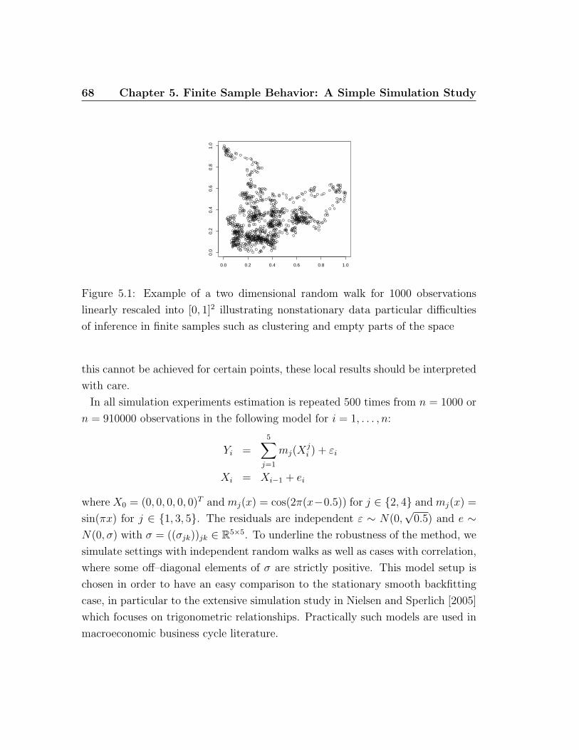
68 Chapter 5. Finite Sample Behavior: A Simple Simulation Study
0.0 0.2 0.4 0.6 0.8 1.0
0.0
0.2
0.4
0.6
0.8
1.0
Figure 5.1: Example of a two dimensional random walk for 1000 observations
linearly rescaled into [0, 1]2 illustrating nonstationary data particular difficulties
of inference in finite samples such as clustering and empty parts of the space
this cannot be achieved for certain points, these local results should be interpreted
with care.
In all simulation experiments estimation is repeated 500 times from n = 1000 or
n = 910000 observations in the following model for i = 1, . . . , n:
Yi =5∑
j=1
mj(Xji ) + εi
Xi = Xi−1 + ei
where X0 = (0, 0, 0, 0, 0)T and mj(x) = cos(2π(x−0.5)) for j ∈ {2, 4} and mj(x) =
sin(πx) for j ∈ {1, 3, 5}. The residuals are independent ε ∼ N(0,√
0.5) and e ∼N(0, σ) with σ = ((σjk))jk ∈ R5×5. To underline the robustness of the method, we
simulate settings with independent random walks as well as cases with correlation,
where some off–diagonal elements of σ are strictly positive. This model setup is
chosen in order to have an easy comparison to the stationary smooth backfitting
case, in particular to the extensive simulation study in Nielsen and Sperlich [2005]
which focuses on trigonometric relationships. Practically such models are used in
macroeconomic business cycle literature.
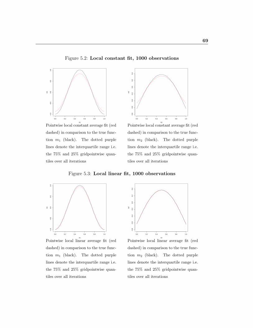
69
Figure 5.2: Local constant fit, 1000 observations
0.0 0.2 0.4 0.6 0.8 1.0
−1.
0−
0.5
0.0
0.5
1.0
X1
m1
Pointwise local constant average fit (red
dashed) in comparison to the true func-
tion m1 (black). The dotted purple
lines denote the interquartile range i.e.
the 75% and 25% gridpointwise quan-
tiles over all iterations
0.0 0.2 0.4 0.6 0.8 1.0
−0.
8−
0.6
−0.
4−
0.2
0.0
0.2
0.4
X2
m2
Pointwise local constant average fit (red
dashed) in comparison to the true func-
tion m2 (black). The dotted purple
lines denote the interquartile range i.e.
the 75% and 25% gridpointwise quan-
tiles over all iterations
Figure 5.3: Local linear fit, 1000 observations
0.0 0.2 0.4 0.6 0.8 1.0
−1.
0−
0.5
0.0
0.5
1.0
X1
m1
Pointwise local linear average fit (red
dashed) in comparison to the true func-
tion m1 (black). The dotted purple
lines denote the interquartile range i.e.
the 75% and 25% gridpointwise quan-
tiles over all iterations
0.0 0.2 0.4 0.6 0.8 1.0
−0.
8−
0.6
−0.
4−
0.2
0.0
0.2
0.4
X2
m2
Pointwise local linear average fit (red
dashed) in comparison to the true func-
tion m2 (black). The dotted purple
lines denote the interquartile range i.e.
the 75% and 25% gridpointwise quan-
tiles over all iterations
70 Chapter 5. Finite Sample Behavior: A Simple Simulation Study
When using kernel smoothing techniques there should be some guideline on how
to choose the smoothing parameter h. This is a largely unsolved problem, since
the admissible rates as stated in the theorems are only asymptotically true. They
are different from the stationary rates, not only with n effectively replaced by
nβ but also in an additional speed restriction from above hj < n−1/5β+−ε. Due to
nonstationarity of the data, the shrinking of the bandwidth h must not only satisfy
a maximum speed as usual but also a minimum speed in order to guarantee enough
data points in the observation window asymptotically. Cross–validation techniques
proved to be useful for finite samples. For simplicity, the bandwidth is chosen via
cross validation for the best componentwise fit, which does not necessarily yield the
same results as for the best global fit, especially when regressors are correlated.
For SBE with stationary data, in Nielsen and Sperlich [2005] a more involved
global cross validation procedure is used without proof which seems to induce an
additional bias of yet unknown size. We found it favorable to use a data adaptive
local choice hj(xj) ∼
(∑i∈Ijk0
1Nxj,k
(Xji ))−1/5
for fixed small k << 1 depending
on the number of visits to a k–neighborhood around xj. For this no preknowledge
of β is required, which in practice must be estimated first, e.g. via a Hill type
estimator from (2.6) suffering from poor convergence properties. Though deriving
formal results for such a local data–driven bandwidth is beyond the scope of this
paper. For a local stochastic bandwidth theoretical results are not straightforward,
as can be seen from Guerre [2004] in the general non–additive model under the
restrictive uniform recurrence assumption. Potentially the theoretical results in
Mammen and Park [2005] for mixing processes via plug–in and penalized least
squares could be extended for β–null Harris recurrent processes.
The implementation closely follows the strategy by Nielsen and Sperlich [2005]
and Haag [2006]. In particular, any steps of the algorithm are performed on a fixed
grid in each direction. Thus the data generating processes are linearly transformed
to live in the cuboid [0, 1]d, for easy comparison. In order to reduce numerical errors
in the integrals, M = 101 equidistant grid points are chosen. For the algorithm to
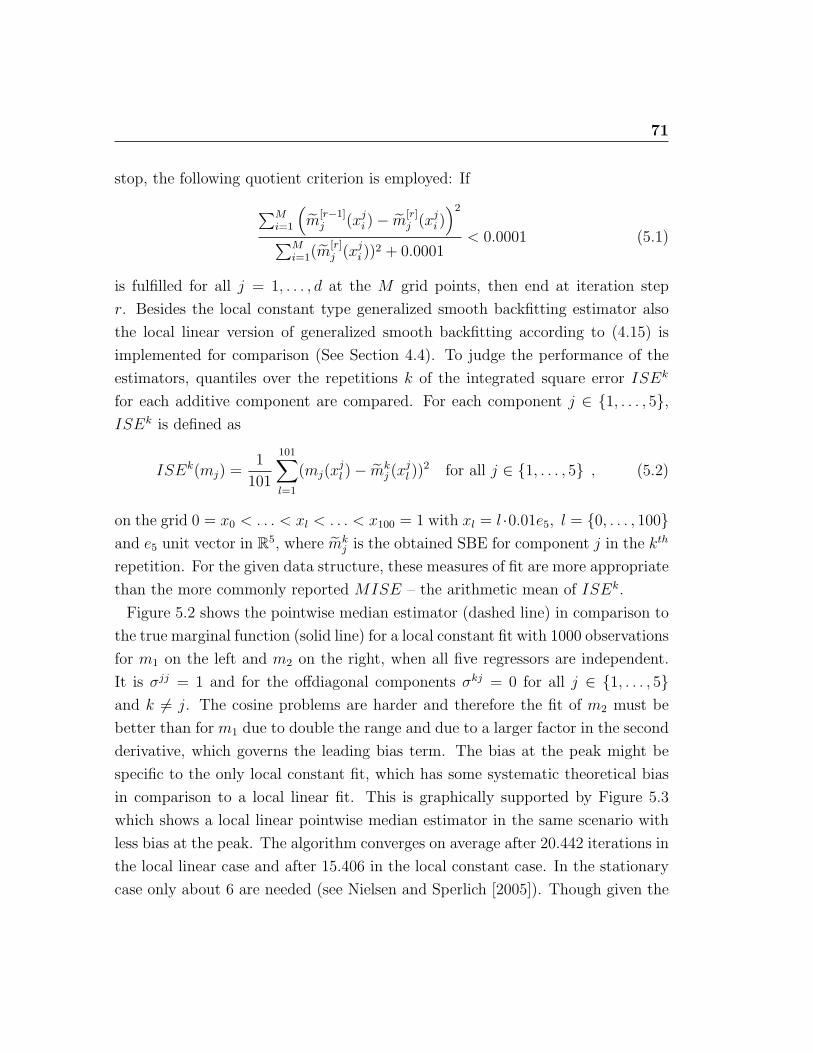
71
stop, the following quotient criterion is employed: If
∑Mi=1
(m
[r−1]j (xj
i )− m[r]j (xj
i ))2
∑Mi=1(m
[r]j (xj
i ))2 + 0.0001
< 0.0001 (5.1)
is fulfilled for all j = 1, . . . , d at the M grid points, then end at iteration step
r. Besides the local constant type generalized smooth backfitting estimator also
the local linear version of generalized smooth backfitting according to (4.15) is
implemented for comparison (See Section 4.4). To judge the performance of the
estimators, quantiles over the repetitions k of the integrated square error ISEk
for each additive component are compared. For each component j ∈ {1, . . . , 5},ISEk is defined as
ISEk(mj) =1
101
101∑l=1
(mj(xjl )− mk
j (xjl ))
2 for all j ∈ {1, . . . , 5} , (5.2)
on the grid 0 = x0 < . . . < xl < . . . < x100 = 1 with xl = l ·0.01e5, l = {0, . . . , 100}and e5 unit vector in R5, where mk
j is the obtained SBE for component j in the kth
repetition. For the given data structure, these measures of fit are more appropriate
than the more commonly reported MISE – the arithmetic mean of ISEk.
Figure 5.2 shows the pointwise median estimator (dashed line) in comparison to
the true marginal function (solid line) for a local constant fit with 1000 observations
for m1 on the left and m2 on the right, when all five regressors are independent.
It is σjj = 1 and for the offdiagonal components σkj = 0 for all j ∈ {1, . . . , 5}and k 6= j. The cosine problems are harder and therefore the fit of m2 must be
better than for m1 due to double the range and due to a larger factor in the second
derivative, which governs the leading bias term. The bias at the peak might be
specific to the only local constant fit, which has some systematic theoretical bias
in comparison to a local linear fit. This is graphically supported by Figure 5.3
which shows a local linear pointwise median estimator in the same scenario with
less bias at the peak. The algorithm converges on average after 20.442 iterations in
the local linear case and after 15.406 in the local constant case. In the stationary
case only about 6 are needed (see Nielsen and Sperlich [2005]). Though given the
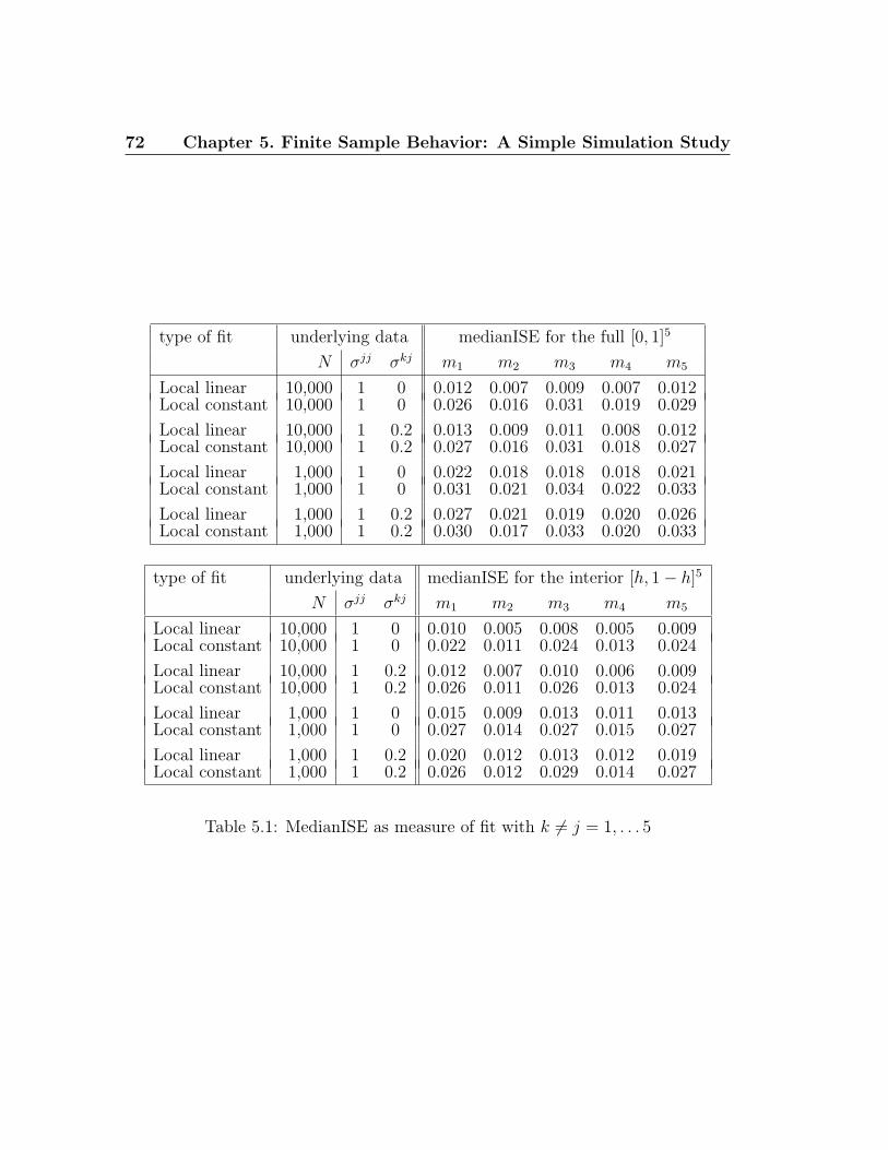
72 Chapter 5. Finite Sample Behavior: A Simple Simulation Study
type of fit underlying data medianISE for the full [0, 1]5
N σjj σkj m1 m2 m3 m4 m5
Local linear 10,000 1 0 0.012 0.007 0.009 0.007 0.012Local constant 10,000 1 0 0.026 0.016 0.031 0.019 0.029
Local linear 10,000 1 0.2 0.013 0.009 0.011 0.008 0.012Local constant 10,000 1 0.2 0.027 0.016 0.031 0.018 0.027
Local linear 1,000 1 0 0.022 0.018 0.018 0.018 0.021Local constant 1,000 1 0 0.031 0.021 0.034 0.022 0.033
Local linear 1,000 1 0.2 0.027 0.021 0.019 0.020 0.026Local constant 1,000 1 0.2 0.030 0.017 0.033 0.020 0.033
type of fit underlying data medianISE for the interior [h, 1− h]5
N σjj σkj m1 m2 m3 m4 m5
Local linear 10,000 1 0 0.010 0.005 0.008 0.005 0.009Local constant 10,000 1 0 0.022 0.011 0.024 0.013 0.024
Local linear 10,000 1 0.2 0.012 0.007 0.010 0.006 0.009Local constant 10,000 1 0.2 0.026 0.011 0.026 0.013 0.024
Local linear 1,000 1 0 0.015 0.009 0.013 0.011 0.013Local constant 1,000 1 0 0.027 0.014 0.027 0.015 0.027
Local linear 1,000 1 0.2 0.020 0.012 0.013 0.012 0.019Local constant 1,000 1 0.2 0.026 0.012 0.029 0.014 0.027
Table 5.1: MedianISE as measure of fit with k 6= j = 1, . . . 5
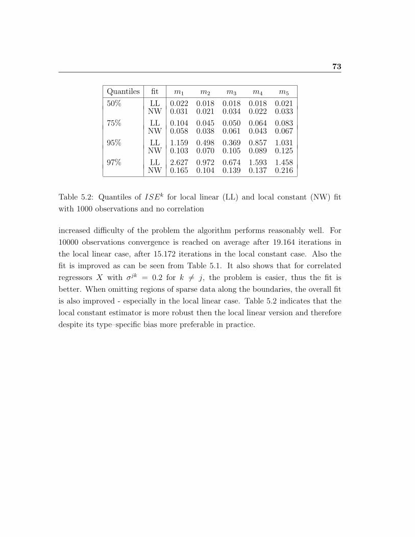
73
Quantiles fit m1 m2 m3 m4 m5
50% LL 0.022 0.018 0.018 0.018 0.021NW 0.031 0.021 0.034 0.022 0.033
75% LL 0.104 0.045 0.050 0.064 0.083NW 0.058 0.038 0.061 0.043 0.067
95% LL 1.159 0.498 0.369 0.857 1.031NW 0.103 0.070 0.105 0.089 0.125
97% LL 2.627 0.972 0.674 1.593 1.458NW 0.165 0.104 0.139 0.137 0.216
Table 5.2: Quantiles of ISEk for local linear (LL) and local constant (NW) fit
with 1000 observations and no correlation
increased difficulty of the problem the algorithm performs reasonably well. For
10000 observations convergence is reached on average after 19.164 iterations in
the local linear case, after 15.172 iterations in the local constant case. Also the
fit is improved as can be seen from Table 5.1. It also shows that for correlated
regressors X with σjk = 0.2 for k 6= j, the problem is easier, thus the fit is
better. When omitting regions of sparse data along the boundaries, the overall fit
is also improved - especially in the local linear case. Table 5.2 indicates that the
local constant estimator is more robust then the local linear version and therefore
despite its type–specific bias more preferable in practice.

74 Chapter 5. Finite Sample Behavior: A Simple Simulation Study
Chapter 6
Conclusion
6.1 Summary
We have introduced a nonparametric estimation procedure, which allows to es-
timate a regression problem with more than d > 2 potentially nonstationary
covariates. As in a stationary setting, estimating an additive model allows to
circumvent the ordinary curse of dimensionality. Thus rate of convergence and
asymptotic variance are of univariate form. Though the added nonstationary diffi-
culty is reflected by the fact that for generalized smooth backfitting the worst case
bivariate type of nonstationarity and the corresponding β govern the rate. For
a model with an arbitrary but potentially large finite amount of regressors and
nonstationarity as an added difficulty, this is the best to be achieved. Under the
other suggested backfitting type methods, we can reach a best additive fit to more
general true models, but require more regularity in the data than pairwise β–null
Harris recurrence and obtain slower rates. Under full β–null Harris recurrence ,
standard smooth backfitting scaled according to full–dimensional objects yields
the best additive approximation a fully general true model.
Furthermore in the special case of a stationary residual ε, results are obtained
which could serve as a starting point for an elegant way of additive nonlinear
cointegration. When each component function is monotone, the desired symme-
try between response and observables as in linear cointegration can be achieved.
76 Chapter 6. Conclusion
While the more general results of Karlsen et al. [2007] are limited to a very small
number of cointegrated components, the method introduced here works for an ar-
bitrary amount of regressors. Therefore in a wide range of applications it might be
the only way to determine a general cointegration relationship between variables
without prespecifying a parametric form.
6.2 Outlook
The suggested methods can be used to test for linearity in cointegration relation-
ships. While a formal testing procedure might prove difficult to develop, estimation
results for a general additive model can already provide a guideline if linearity is
appropriate or if not, what kind of nonlinearity should be modeled. In economic
models where a cointegration relationship is expected, but could not be detected
with existing methods, estimation with GSBE could help to provide empirical ev-
idence for economic intuition. This especially applies to purchasing power parity
(PPP) or term structure models as in Tsay [2002] Section 2.9. It might be of in-
terest to develop model specification tests in this general scenario generalizing the
cointegration rank test of Johansen [1991]. Furthermore it might be interesting to
investigate how detrending of data with a deterministic trend should be done in
order to obtain similar results for resulting β–null Harris recurrent observations
as presented here. One could also think of deriving least squares type estimators
under more smoothness or parametric assumptions and β–null Harris recurrent
data. Though the framework is tailored for local smoothing techniques. Thus
aiming for a global fit seems somehow unnatural and will always suffer from the
nonstationary curse of dimensionality.
Presented techniques can serve to provide nonparametric estimates of the indi-
vidual marginal utility function in Euler equations. They characterize intertem-
poral optimization and are driven by nonstationary individual consumption (See
e.g. Cochrane [2001]). Up to now estimation in this central economic question has
been dominated by parametric GMM methods leading to sometimes contradictory
results.
6.2 Outlook 77
Generally, β–null Harris recurrence delivers a natural blocksize of independent
blocks of sums of observations between recurrence times (See Appendix A.1). This
might serve as a way to generalize block bootstrap procedures in time series (see
Hall et al. [2003]) to the recurrent setting. With this the usually somewhat ar-
bitrary block window has a stochastic meaning and might be estimable for Feller
type processes.
If observations are discrete, null–Harris recurrence and positive Harris recurrence
coincide. Therefore all measures are finite and estimation is much easier resulting
in simpler assumptions. This might be applicable to storage or queuing models.

78 Chapter 6. Conclusion
Appendix A
A.1 Markov Theory
To keep the paper as self–contained as possible, essential notions and results of
Markov theory relevant for the understanding of the paper shall be mentioned.
A.1.1 Split Chain and Invariant Measure
Every φ irreducible Markov chain (Xi)i satisfies the minorization inequality. That
means, for any such (Xi)i there exists a small function s, a probability measure ν
and an integer m0 ≥ 1 such that
Pm0 ≥ s⊗ ν .
Without much loss of generality we assume throughout the paper that m0 = 1,
i.e. the minorization inequality has the form:
P ≥ s⊗ ν , (A.1)
where s and ν are small and ν(Rn) = 1. In particular it is 0 ≤ s(x) ≤ 1 for x ∈ Rn.
If (A.1) holds, then the pair (s, ν) is called a pseudo–atom for P . Note that ν is
independent of x. This is the basis for constructing the corresponding split chain
of (Xi)i.
80 Chapter A. Appendix
From (A.1) we derive:
P (x, A) = (P (x, A)− s(x)ν(A)) + s(x)ν(A)
= (1− s(x))
[(P (x, A)− s(x)ν(A)
1− s(x)
)1{s(x)<1} + 1a(x)1{s(x)=1}
]+ s(x)ν(A)
=: (1− s(x)) Q(x, A) + s(x)ν(A)
Hence the transition probability P can be thought of as a convex combination of
a transition probability Q and the independent small measure ν. Thus the chain
regenerates each time ν is chosen – which occurs with probability s(x). Introducing
the split chain (Xi, Yi) helps to formalize this observation. The auxiliary chain Yi
only takes on values 0 and 1. For Xi = x and Yi−1 = yi−1, the auxiliary chain {Yt}takes on the value 1 with probability s(x). Thus α = Rn × {1} is a proper atom
for the split chain. Denote by
τ0 := min {i ≥ 1 : Yi = 1} (A.2)
the corresponding recurrence time. We will frequently need the consecutive se-
quence of recurrence times (τk)∞k=−1 starting in t = 0 defined recursively by:
τk := min {i ≥ τk−1 : Yi = 1} , (A.3)
with starting value set as τ−1 := −1 (any negative number would do). Write
τ0 = τα = τ for the first recurrence time with respect to the pseudo atom α.
Furthermore denote the number of regenerations up to n by
T (n) = maxk{k : τk ≤ n} (A.4)
We need for scaling purposes
TC(n) =n∑
i=1
1C(Xi)
a(n) = Eλ(TC(n))
πs(C), (A.5)
with λ any initial distribution and C a so called D–set, such that (A.5) is always
well defined. Any small set is a D–set and the definition of a does not depend on
A.1 Markov Theory 81
the specific choice of C. It can be easily shown that the invariant measure πs has
a kernel representation in terms of the atom (see [Nummelin, 1984], page 63f)
πs := ν Gs,ν , with Gs,ν :=∞∑
t=0
(P − s⊗ ν)t . (A.6)
Note that for ease of exposition in the main text, we omit the index s in πs. Then
for g ∈ L1πs
(Rd, R) it follows
Gs,νg(x) = E
[τ∑
i=0
g(Xi)|X0 = x
]= Ex
[τ∑
i=0
g(Xi)
]. (A.7)
Hence for g = 1A it is πs(A) = νGs,ν1A. If the measure πs is absolutely continuous
w.r.t. Lebesgue measure, we also denote the corresponding density by πs. Then
πs(x)dx = πs(dx). With this define the density πC(x) = πs(x)πs1C
for x ∈ C with C
small.
The minorization inequality and the accompanying split chain permit a decom-
position of the chain into separate and identical parts defined by regeneration
points.
Sn(g) :=n∑
i=0
g(Xi) = U0 +
T (n)∑k=0
Uk + U(n) for any g ∈ L1πs
(Rd, R) , (A.8)
where:
Uk =
{ ∑τk
i=τk−1+1 g(Xi) when k ≥ 0∑ni=τT (n)+1
g(Xi) when k = (n)(A.9)
The sequence {(Uk, (τk − τk−1))}∞k=1 consists of independent identically distributed
(iid) random variables. Denote the common marginal distribution of Uk with
U = U(g) and respectively µ = µ(gh) = EU(gh) = πs(gh) and σ = σ(gh) = VU(gh).
A.1.2 β–null Harris recurrence
The definitions in (2.4) and (2.6) are equivalent. Under β–Harris recurrence for
n −→ ∞ it is asymptotically a(n) ∼ nβLs(n) with Ls(n) from the tail condition

82 Chapter A. Appendix
of the recurrence time (2.6) slowly varying at infinity. Furthermore the exact
asymptotic distribution can be specified (see e.g.Chen [2000] Theorem 1.3.)
(a(n))−1/2
n∑i=1
1C(Xi)f(Xi) ∼ σf√
gβ N (0, 1) (A.10)
with σf =∫
f 2(x)πC(x) dx + 2∑∞
i=0
∫f(x)P if(x)πC(x) dx where (A.10) is only
defined for such functions f for which σf exists. The random variable gβ is inde-
pendent of the normal distribution and is Mittag–Leffler Mβ distributed.
A.1.3 The Quotient Limit Theorem
The following result is the appropriate generalization of ergodicity to Harris recur-
rent Markov chains.
Theorem A.1. If a discrete Markov process (Xi)i is Harris recurrent, then for
any functions f, g ∈ L1π =
{φ|∫
φ(x)π(dx) < ∞}
with∫
g(x)π(dx) 6= 0 it is
limn−→∞
∑ni=1 f(Xi)∑ni=1 g(Xi)
=
∫f(x)π(dx)∫g(x)π(dx)
P− a.s . (A.11)
A.2 Proofs
This section is split into three main subsections. In the first part, operator notation
for the backfitting procedure is introduced to motivate the proofs in subsection two.
In the second part, necessary uniform lemmas are proven which are the main tools
for the proofs of the main theorems in subsection three.
A.2.1 On the Structural Form of Generalized Smooth
Backfitting
For simplification rewrite the generalized backfitting problem (3.6) in form of an
operator equation in the corresponding pairwise Hilbert spaces L2πjk
. This reveals
and emphasizes the underlying structure of the problem and gives fundamental

A.2 Proofs 83
insights for its understanding and proof. Structurally we obtain an inverse problem
— which in contrast to many other situations is well–posed 1. Componentwise in
j = 1, . . . , d we get with boundary modified kernels (2.24):
mj(xj) =
∑k 6=j
1
d− 1(1k − Φjk)mj(x
j)− [Aj,kmk](xj) (A.12)
with centering operator operators Φjk and projection operators Aj,k and 1k defined
as
1kmj(xj) = m
(k)j (xj) (A.13)
Φjkmj(xj) =
∫m
(k)j (xj)π
(k)j (xj)dxj∫
π(k)j (xj)dxj
=1
T jk(n)
∑i∈Ijk
Yi
[Aj,kfk
](xj) =
∫fk(x
k)πj,k(x
j, xk)
π(k)j (xj)
dxk for j 6= k ,
for fk : R → R. Note that∑
k 6=j Φjkmj(xj) only differs from zero when (3.8) is
not fulfilled. For rectangular Gj and boundary kernels it is∑
k 6=j Φjkmj(xj) = 0.
The operator Aj,k projects any f ∈ H(j)k = L2
π(j)k
onto H(k)j . Thus Aj :=
∑k 6=j Aj,k
projects any f ∈ H(k)−j onto Hj. Thus for any component j there is a a suitable
space of additive functions H(j) composed of pairwise coordinatewise projections
H(j)k of (3.11) with H(j) =
⊕dj=1H
(j)k .
Introducing vector notation m = (m1(x1), . . . , md(x
d))T ∈ Rd and analogously
m = (m1(x1), . . . , md(x
d))T ∈ Rd we obtain the simplest form in matrix notion
(I − A)m =1
d− 1(1− Φ)m (A.14)
with I the identity and, under Assumptions 1-2 or 1 and 4, compact operator
1Compare in contrast the case of ill–posed inverse problems. See Carrasco, Florens andRenault for a survey article on ill–posed inverse problems [Carrasco et al., 2003]
84 Chapter A. Appendix
matrices
Φ =
0 Φ1,2 . . . Φ1,d−1 Φ1,d
Φ2,1 0 Φ2,3 . . . Φ2,d
.... . .
...
Φd−1,1 . . . Φd−1,d−2 0 Φd−1,d
Φd,1 Φd,2 . . . Φd,d−1 0
1 =
0 12 . . . 1d−1 1d
11 0 13 . . . 1d
.... . .
...
11 . . . 1d−2 0 1d
11 12 . . . 1d−1 0
A = −
0 A1,2 . . . A1,d−1 A1,d
A2,1 0 A2,3 . . . A2,d
.... . .
...
Ad−1,1 . . . Ad−1,d−2 0 Ad−1,d
Ad,1 Ad,2 . . . Ad,d−1 0
=
0 −Aup
. . .
−Adown 0
.(A.15)
Simplifying notation in (A.14) we can also write:
(I − A)m = mII (A.16)
with mII = 1d−1
(∑
k 6=1 1km1(x1), . . . ,
∑k 6=d 1kmd(x
d))T ∈ Rd. And by setting
m0 =∑d
j=11
d−1
∑k 6=j
1T jk(n)
∑i∈Ijk
Yi the centering term can be omitted. In the
case of a fully–recurrent vector of covariates and notation as introduced in (3.2),
the generalized backfitting equations (A.16) reduce to the standard backfitting
operator equation with projections in L2π as in [Mammen et al., 1999].
Since for any sample size n, A is compact and self–adjoint, this is a Fredholm
equation of the second kind. Formally, in order to find a solution m, the inverse
of I − A must be applied to (A.14). For this the operator must be injective,
thus the null space N (I − A) of the operator has to be trivial. This is achieved
through the sample counterparts of normalization condition (3.18). According
to Fredholm and Riesz theory in functional analysis a solution to (A.14) exists, if
(I−Φ)m is in the range of the closure of (I−A) which is identical to the orthogonal
complement N (I − A∗) = N (I − A) as A is self adjoint. Since this null space is
trivial under the norming constraint, a solution exists and is unique. To obtain
a practical solution, however, show that (I − A) is a contraction operator. Then
according to a generalized version of Banach’s fixed–point theorem the unique
A.2 Proofs 85
solution is reached through an iterative procedure and its rate of convergence will
be geometric. In matrix notation the SBE algorithm works as given right below.
Instead of iterating the full A, the matrix is split into upper and lower triangular
part. Then Aup projects mj from the previous iteration step, while Adown treats
already updated versions of the estimator components from within the rth iteration
step.
m[r] = mII −
0 Aup
. . .
0 0
m[r−1] −
0 0. . .
Adown 0
m[r] (A.17)
However, what complicates the following proof of the asymptotic results is that
all operators are estimated depending on the sample size n. Therefore in order
to ensure that the obtained m from (A.17), is also the solution to the original
additive regression problem (1.1) under the norming constraint (3.8) some uniform
convergence results are needed. Since in the null-recurrent setting these are not
available in the existing literature, they are shown in the following section.
A.2.2 Preliminary Lemmata
In order to prove any of the theorems, first, some preliminary technical lemmata
with uniform convergence results need to be shown. These are not only essential
for the proofs but also of interest on their own.
Uniform consistency of the Kernel invariant density estimate
To our knowledge in the general case of β–null Harris recurrent processes uniform
results for consistency have not been established. While for subcases with finite
invariant measure, a Hoeffding type exponential inequality exists (see [Glynn and
Ormoneit, 2002]), the proof of the general case is more involved.
Although for smooth backfitting only univariate and pairwise bivariate density
estimates are of interest, the following proof is given for d covariates. To ease
notation, indices and superscripts indicating components to be marginal j or jk
specific will be generally omitted. We need the following moment bounds:
86 Chapter A. Appendix
Lemma A.1. Let Assumptions 1-2 hold. Set Kx(u) = hdKx,h(u) = K((u−x)/h).
Let the process start in a point of regeneration and set U = U0 =∑τ0
i=0 Kx,h(Xi).
Then it is with −∞ < µ, µ′< ∞ and 0 < σ, σ′< ∞
µ(Kx,h) = EU(Kx,h) = π(Kx,h) = µ + o(1)
µ(|Kx,h|) = EU(|Kx,h|) = π(|Kx,h|) = µ′ + o(1)
hdσ2(Kx,h) = hd(EU2(Kx,h)− µ2(Kx,h)
)= σ2 + o(1)
hdσ2(|Kx,h|) = hd(EU2(|Kx,h|)− µ2(|Kx,h|)
)= σ′2 + o(1)
σ2(Kx) = EU2(Kx)− µ2(Kx) = σ2 .
Proof. See Lemma 5.1. and 5.2. in Karlsen and Tjøstheim [2001] for the proof
of the bounds. The form of σ follows from Theorem 5.3. hdσ2(Kx,h) =∫
πC(x +
hu)K2(u) du + 2∫
K(u)PGs,νKx,h(x + hu) + o(1).
Assume w.l.o.g. that the process starts in a point of regeneration. The proof
is on the atomic level, but extends straightforwardly to small sets. The Green
function a(n) is defined in (A.5).
Lemma A.2 (Uniform consistency of the Kernel density estimator).
Let Assumptions 1-2 hold. Then choose a bandwidth h → 0 such that√a( n
L2a(n))L2a(n)hd →∞ and set h l(n)1/d =
√a(
nL2(a(n))
)L2(a(n)) . Then
supx∈Gh
|π(x)− π(x)| = OP
h2 +1
hd
√a(
nL2(a(n))
)L2(a(n))
(A.18)
supx∈∂Gh
|π(x)− π(x)| = OP
h +1
hd
√a(
nL2(a(n))
)L2(a(n))
. (A.19)
A.2 Proofs 87
Proof. It is sufficient to show that for given
cn = h2 +1
hd
√a(
nL2(a(n))
)L2(a(n))
c′n = h +1
hd
√a(
nL2(a(n))
)L2(a(n))
it is that for all η, η′ > 0 there exist constants c, c′ > 0 such that
supn
P
(supx∈G
|π(x)− π(x)| ≥ c · cn
)= η
supn
P(
supx∈∂G
|π(x)− π(x)| ≥ c′ · c′n)
= η′ .
In fact we will even show almost sure convergence.
To shorten notation we will write cn instead of c · cn and keep in mind that cn is
simply the rate without any constants. The same holds for c′n.
Split up into variance and bias part. For the interior Gh it is:
P
(supx∈Gh
|π(x)− π(x)| ≥ cn
)
≤ P
(supx∈Gh
|π(x)− µ(Kx,h)|+ supx∈Gh
|µ(Kx,h)− π(x)| ≥ cn
)
≤ P
(supx∈Gh
|π(x)− µ(Kx,h)| ≥cn
2
)+ P
(supx∈Gh
|µ(Kx,h)− π(x)| ≥ cn
2
)= Si
1 + Si2 ,
Since G ⊂ Rd is compact and hence bounded, we have to be careful at the bound-
ary. For the C1h-ring-boundary ∂Gh we get:
P(
supx∈∂Gh
∣∣∣∣π(x)− π(x)
∫G
Kh,x(u)du
∣∣∣∣ ≥ cn
)≤ P
(sup
x∈∂Gh
|π(x)− µ(Kx,h)| ≥cn
2
)+ P
(sup
x∈∂Gh
∣∣∣∣µ(Kx,h)− π(x)
∫G
Kh,x(u)du
∣∣∣∣ ≥ cn
2
)= Sb
1 + Sb2 ,
88 Chapter A. Appendix
For the bias parts Si2 and Sb
2, standard analysis with the usual kernel arguments
carries over. Since we have for x in the interior GC1h that∫G Kh,x(u)du = 1, we
can treat Si2 and Sb
2 together:
µ(Kx,h)− π(x)
∫G
Kh,x(u)du =
∫Bx(C1h)∩G
(π(x + hu)− π(x))K(u)du
=d
dx(π(x)) h
∫Bx(C1h)∩G
uK(u)du + O(h2)
=
{O(h2) for x ∈ Gh
O(h) for x ∈ ∂Gh
,
since for x ∈ ∂Gh the ball Bx(C1h) is not entirely in G. Thus the with symmetry
of the kernel the integral is not zero as in the case for x in the interior.
Now treat the stochastic term S1 = P(supx∈G |π(x)− µ(Kx,h)| ≥ cn
2
). Here we
do not have to distinguish between cases of x on the boundary or not. As G is
compact, there exists a cover of l(n) open balls I1, . . . , Ik, . . . , Il(n) with radiusc1
l(n)1/d for an appropriate constant c1 and with centers in xk and⋃l(n)
k=1 Ik ⊇ G.
The maximal distance attainable between elements inside one of the balls is the
diameter:
maxa,b∈Ik
‖a− b‖ ≤ 2c1
l(n)1/d=
c
l(n)1/dfor all k ∈ {1, . . . , l(n)} (A.20)
P(
supx∈G
|π(x)− µ(Kx,h)| ≥cn
2
)= P
(max
1≤k≤l(n)sup
x∈G∩Ik
|π(x)− µ(Kx,h)| ≥cn
2
)≤ P
(max
1≤k≤l(n)sup
x∈G∩Ik
|π(x)− π(xk)| ≥cn
6
)+ P
(max
1≤k≤l(n)|π(xk)− µ(Kxk,h)| ≥
cn
6
)+P(
max1≤k≤l(n)
supx∈G∩Ik
|µ(Kxk,h)− µ(Kx,h)| ≥cn
6
)= Q1 + Q2 + Q3
The first and the third term, Q1 and Q3, are easy to handle and therefore treated
A.2 Proofs 89
first. Look at Q1:
supx∈G∩Ik
|π(x)− π(xk)| =1
T (n)sup
x∈G∩Ik
∣∣∣∣∣n∑
i=1
(Kh,x(Xi)−Kh,xk(Xi))(Xi)
∣∣∣∣∣=
1
π(G)
∫G
supx∈G∩Ik
|Kh,x(u)−Kh,xk(u)|π(u)du P− a.s.
≤ supx∈G∩Ik
L
hd+1n
‖x− xk‖ P− a.s.
≤ Lc1
hd+1n l(n)1/d
P− a.s. .
The first P − a.s relation is a consequence of the quotient limit theorem (A.11),
while the inequalities thereafter follow directly from (A.20) and the Lipschitz as-
sumption on the kernel.
Since the integral operator and everything inside is continuous, obviously we
also get max1≤k≤l(n) supx∈G∩Ik|µ(Kxk,h)− µ(Kx,h)| = O
(1
hd+1n l(n)1/d
). Thus when
imposing c := O(
1
hd+1n l(n)1/d
), then Q1 and Q3 are oP (1).
Q2, the second term, however, needs some extra considerations: On the grid of
the xk-balls we can simplify the expression by the triangle inequality and get an
upper bound where “the maximum is outside the measure” and therefore easier
tractable:
P(
max1≤k≤l(n)
|π(xk)− µ(Kxk,h)| ≥cn
6
)= P
(max
1≤k≤l(n)
∣∣∣∣∣ 1
T (n)
n∑i=1
Kxk,h − µ(Kxk,h)
∣∣∣∣∣ ≥ cn
6
)
≤ l(n) · supx∈G
P
(∣∣∣∣∣ 1
T (n)
n∑i=1
Kx,h − µ(Kx,h)
∣∣∣∣∣ ≥ cn
6
)
≤ l(n) · supx∈G
P
∣∣∣∣∣∣ 1
T (n)hd
T (n)−1∑k=0
Wk,x + U(n)
∣∣∣∣∣∣ ≥ c′n
90 Chapter A. Appendix
≤ l(n) · supx∈G
P
1
T (n)hd
∣∣∣∣∣∣T (n)−1∑
k=0
Wk,x
∣∣∣∣∣∣ ≥ c′′n
,
where the second to last inequality follows because of with c′n = cnπs(C)6
. Since
c′′n differs from cn only by a constant, we continue notation with cn. Furthermore
the sum is rewritten in terms of the centered split chain components W ′k,x =
Ux,k − µ(Kx) where Ux,k is the k–th component of the split chain of Kx. Thus it
is:
Ux,k =
τk+1∑j=τk+1
Kx(Xj) for k = 0, . . . , T (n)− 1
Un =n∑
j=τT (n)+1
Kx(Xj)
As parts of a split chain all Wx,k are iid Wx for a given x ∈ G. And obviously from
the definition it is E(Wx) = 0.
When dealing with P(∣∣∣ 1
T (n)
∑T (n)−1k=0 Wk,x
∣∣∣ ≥ cn
6
)the main difficulty stems from
the fact that the norming TC(n) is stochastic and not independent of Wx. It is
P
1
T (n)hd
∣∣∣∣∣∣T (n)−1∑
k=0
Wk,x
∣∣∣∣∣∣ ≥ cn
≤ P
1
T (n)
∣∣∣∣∣∣T (n)−1∑
k=0
Wk,x
∣∣∣∣∣∣ ≥ cnhd, 1 ≤ T (n) ≤ δn
+P
1
T (n)hd
∣∣∣∣∣∣T (n)−1∑
k=0
Wk,x
∣∣∣∣∣∣ ≥ cn, T (n) > δn
≤ P
∣∣∣∣∣∣T (n)−1∑
k=0
Wk,x
∣∣∣∣∣∣ ≥ cnδnhd
A.2 Proofs 91
The last inequality follows since for the first term
P
1
T (n)
∣∣∣∣∣∣T (n)−1∑
k=0
Wk,x
∣∣∣∣∣∣ ≥ cnhd, 1 ≤ T (n) ≤ δn
≤ P
(T (n) ≤ δnκ
hdcn
, 1 ≤ T (n) ≤ δn
)≤ P (T (n) ≤ δn) = P
(T (n) ≤ ln
δn
ln
)≤
2lna( δn
ln)− 1
(ln + 1)a( δn
ln) + 1
→ 0
with κ = max1≤k≤δn |Uk − µ| < ∞ and ln → 0 chosen such that2lna( δn
ln)−1
(ln+1)a( δnln
)+1→ 0
at polynomial rate n−α with α such that l(n)n−α ∼ n−α′ and α′ > 1. The last
inequality follows from Theorem 2.1. in [Chen, 1999a].
Treat the remaining second term:
ξk = Uk1|Uk|≤R − E(Uk1|Uk|≤R)
ηk = Uk1|Uk|>R − E(Uk1|Uk|>R)
with R > 0 large enough such that Eξ2 := σ2R > 0. Then Wk = ξk + ηk.
For each n, T (n) is a stopping time w.r.t to the iid sequence ξk. With a standard
maximal inequality for martingales (see e.g. Theorem 2.1., Chapter2, [Hall and
Heyde, 1980])
P
∣∣∣∣∣∣T (n)−1∑
k=0
ξk
∣∣∣∣∣∣ ≥ cnδnhd
≤ P
(maxl≤T (n)
∣∣∣∣∣l∑
k=0
ξk
∣∣∣∣∣ ≥ cnδnhd
)
≤ e−λL2a(n)θE
exp θ
∣∣∣∣∣∣T (n)∑k=0
ξk√a( n
L2a(n))
∣∣∣∣∣∣(A.21)
For cnδnhd = λ
√a( n
L2a(n))L2a(n) with λ > 0 and θ > 0 arbitrary. The separation
into weighting and exponential factors seems at this stage somehow arbitrary. But
their choice is perfectly balanced in view of the following assessment.
With Lemma 2.2. in [Chen, 2000], which uses that the left hand side of the
expression below is a martingale where the optional stopping theorem can be
92 Chapter A. Appendix
applied to:
E
exp θ
∣∣∣∣∣∣T (n)−1∑
k=0
ξk√a( n
L2a(n))− (T (n) + 1)Ln(s, θ)
∣∣∣∣∣∣
≤ exp
s(1 + ε)L2a(n) +Rθ√
a( nL2a(n)
)
= (1 + o(1)) exp (s(1 + ε)L2a(n)) (A.22)
with s > Λβ(θ), ε > 0 where Λβ(θ) =(Γ(β + 1)
θ2σ2R
2
)1/β
for 0 < β ≤ 1 and
Ln(s, θ) = log E
expθξ√
a( nL2a(n)
)− sL2a(n)
nmin (τα, nε)
≤ log E
expθξ√
a( nL2a(n)
)− sL2a(n)
nτα
+ O(e−εnP (τα ≥ εn))
∼ 1√a( n
L2a(n))
(θ2σ2
R
2− sβ
Γ(β + 1)
)for n →∞ . (A.23)
Thus with (A.22) and (A.23) for n large and s → Λβ(θ), ε → 0:
E
exp θ
∣∣∣∣∣∣T (n)−1∑
k=0
ξk√a( n
L2a(n))
∣∣∣∣∣∣ ≤ exp (Λβ(θ)L2a(n)) .
The inequality above is also true in the case β = 0 if we set Λβ(0) =0 if θ2σ2R ≤ 2
∞ if θ2σ2R > 2
and take s → 0 in (A.22) and (A.23).
In total putting the above inequality into (A.21) and since ξT (n) ≤ 2R
P
∣∣∣∣∣∣T (n)∑k=0
ξk
∣∣∣∣∣∣ ≥ λ
√a(
n
L2a(n))L2a(n)
≤ e−Λ?β(λ)L2a(n) (A.24)
A.2 Proofs 93
with Λ?β(λ) = supθ>0 (λθ − Λβ(θ)) = (2 − β)
(ββλ2
2Γ(β+1)σ2R
) 12−β
by solving the op-
timization for all λ ∈ R and with the convention 00 = 1 in the case β = 0.
Set νk := inf{
n : a(
nL2(a(n))
)≥ k2k
}. Then L2(a(νk)) = log(2k log k). Thus the
right–hand side of (A.24) is summable over k for λ >√
2Γ(β+1)σ2R
(2−β)(2−β)ββ . With Borel-
Cantelli lemma we find :
lim supn→∞
∣∣∣∣∣∣T (n)∑k=0
ξk
∣∣∣∣∣∣ ≤ λ
√a(
n
L2a(n))L2a(n) a.s. (A.25)
For ηk the situation is more standard. According to the Hartmann-Winter’s law
of iterated logarithm it is:
lim supn→∞
maxk≤n−1
∣∣∣∣∣l∑
k=0
ηk
∣∣∣∣∣ ≤√nL2(n)√
Eη2 a.s. .
This implies
lim supn→∞
maxk≤T (n)−1
∣∣∣∣∣l∑
k=0
ηk
∣∣∣∣∣ ≤√T (n)L2(T (n))√
Eη2 a.s. .
But since lim supn→∞ T (n) ≤ κ√
a( nL2a(n)
)L2a(n) a.s. with κ > 0 (Theorem 2.2
in [Chen, 1999a]), we get:
lim supn→∞
maxk≤T (n)−1
∣∣∣∣∣l∑
k=0
ηk
∣∣∣∣∣ ≤√2κEη2
√a(
n
L2a(n))L2a(n) a.s. .
Take R →∞, which yields σ2R → σ2 but σ2
R ≤ σ2 and Eη2 → 0. So finally with
cnδnhd > 6
√2Γ(β + 1)σ2
(2− β)(2−β)ββ
√a(
n
L2a(n))L2a(n)
= Cβσ
√a(
n
L2a(n))L2a(n) , (A.26)
we find that for n large enough it is
l(n) · supx∈G
P
(1
T (n)
∣∣∣∣∣n∑
i=0
Wx,i
∣∣∣∣∣ ≥ cn
6
)= 0 ,
94 Chapter A. Appendix
due to (A.25). In particular the probabilities are summable, i.e.
∞∑k=1
l(n)P
(1
T (n)
∣∣∣∣∣n∑
i=0
Wx,i
∣∣∣∣∣ ≥ cn
6
)< ∞ .
Thus with the Borel–Cantelli lemma we can conclude that the entire term S1 is
o(1) for appropriate choices of cn, δn, h in accordance with (A.26).
For all terms including S2 to vanish, we need additionally (l(n))1/dhd+1 → ∞and hd
√a( n
L2a(n))L2a(n) → ∞. Choose δn = a
(n
L2a(n)
)L2a(n)2 < n. Then the
condition for S2 and (A.26) are simultaneously satisfied for c′n = 1√a( n
L2a(n))L2a(n)hd .
Combining this with the bias term, we find the stated final rates.
Remark A.1.
1. Under the assumption that for any x ∈ G there exists a measure φ such that
Px(Xm ∈ A) ≥ λφ(A) (A.27)
for any A ⊂ C, we could also work with a Markov process version of Ho-
effding’s inequality obtained by Glynn and Ormoneit [Glynn and Ormoneit,
2002]. Together with the usual blocking argument we would find:
P
(1
TC(n)hd
n∑i=0
Wk,x ≥cn
6
)≤ c(a(n)hd)−2 (A.28)
with c > 0 constant and a faster rate cn. But the uniformity imposed
by (A.27) is quite restrictive. It restricts the set of β–recurrent processes
significantly to the positive recurrent ones only.
2. For β = 1, a refinement of the law of iterated logarithm inequality (A.25)
can be found directly in [Chen, 1999a]:
lim supn→∞
∑nk=1 f(Xk)√2nL2n
= σf a.s. . (A.29)
Lemma A.2 is for the full dimensional β–null Harris recurrent process. For the
SBE algorithm, however, only univariate and bivariate results are of importance.
A.2 Proofs 95
Therefore the following corollary is stated for these cases in the generalized SBE
algorithm, extending the result of A.2 to small sets. Assume w.l.o.g. that π(1G) =
1 . Then πG(x) = π(x)π(1G)
= π(x).
Corollary A.2. Assume that Assumptions 2.1 and 4.3 hold. Set β2 := βjk + ε2
with ε2 very small such that max {m : LK(m) ≥ mε2} >> 1 with LK the slowly
varying function from the β–recurrence condition in (2.4) with respect to the bivari-
ate Kernel function K2. Let the bandwidth h → 0 such that nβ22 (L2n
β2)1−β2h2 →∞and set h l(n)1/2 = n
β22 (L2n
β2)1−β2 . Then
supxj,k∈Gj,k
h
∣∣πjk,Gjk(xjk)− πjk,Gjk(xjk)
∣∣ = OP
(h2 +
1
nβ22 (L2nβ2)1−β2h2
)(A.30)
supxj,k∈∂Gj,k
h
∣∣πjk,Gjk(xjk)− πjk,Gjk(xjk)
∣∣ = OP
(h +
1
nβ22 (L2nβ2)1−β2h2
). (A.31)
and
supxj∈G(k)
j,h
∣∣∣∣π(k)
j,G(k)j
(xj)− πj,G(k)
j(xj)
∣∣∣∣ = OP
(h2 +
1
nβ22 (L2nβ2)1−β2h
)(A.32)
supxj,k∈∂Gj,h
∣∣∣∣π(k)
j,G(k)j
(xj)− π(k)
j,G(k)j
(xj)
∣∣∣∣ = OP
(h +
1
nβ22 (L2nβ2)1−β2h
). (A.33)
Proof. The proof is an immediate consequence of the previous lemma and (A.5).
Remark A.2. Analogous results hold for πjk,Gfjk
and πj,Gfj
with full–dimensional
type of nonstationarity β under Assumptions 2.1 and 4.1.
Uniform consistency of the regression function
The one–dimensional pilot smoothers can be decomposed into a bias and a stochas-
tic part as our underlying model (1.1) has an additively separable error term.
mj(xj) =
∑ni=1 Kh,xj(Xj
i )Yi∑ni=1 Kh,xj(Xj
i )
96 Chapter A. Appendix
=
(∑ni=1 Kh,xj(Xj
i )mi(Xi)∑ni=1 Kh,xj(Xj
i )
)+
(∑ni=1 Kh,xj(Xj
i )εi∑ni=1 Kh,xj(Xj
i )
)=: mB
j (xj) + mAj (xj)
Obviously mAj (xj) is the stochastic part whereas mB
j (xj) is the bias or expectation
part.
When starting the SBE algorithm with these pilot estimates we find that the
resulting mj(xj) preserve the additive structure of separate bias and stochastic
part. Thus we have
mj(xj) = mB
j (xj) + mAj (xj) , (A.34)
where each of the parts msj(x
j) with s ∈ {A, B} separately solves the defining
equations (3.2):
msj(x
j) = msj(x
j)− ms0,j −
∑k 6=j
∫ms
k(xk)
πj,k(xj, xk)
πj(xj)dxk (A.35)
with for j 6= k :
ms0,j =
∫ms
j(xj)πj(x
j)dxj∫πj(xj)dxj
.
Definition A.1. Instead of the usual conditional expectation, we need an adapta-
tion which only involves one and two dimensional covariates. The notation follows
from (A.14)
(Am)j(xj) := mj(x
j) +∑k 6=j
∫Gk
mk(xk)
πjk(xjk)
πj(xj)dxk (A.36)
In nonstationary smooth backfitting, Nadaraya–Watson estimates are at least of
two dimensional nonstationary type, i.e. m(k)j or mf
j are of interest.
A.2 Proofs 97
Lemma A.3 (Uniform rate of the bias part). Let either Assumptions 1-3 or As-
sumptions 1,2, and 3* hold.
supxj∈Gf
j,h
∣∣∣mf,Bj (xj)− (Amf )j(x
j)∣∣∣ = OP
(h2 +
1
nβ/2(L2nβ)1−βh
)sup
xj∈∂Gfj,h
∣∣∣mf,Bj (xj)− (Amf )j(x
j)∣∣∣ = OP
(h +
1
nβ/2(L2nβ)1−βh
)
Proof. With standard kernel calculations it is E(mB
j (xj)|Xj1 , . . . , X
jn
)=
(Am)j(xj) + O(h2) uniformly in the interior Gj and E
(mB
j (xj)|Xj1 , . . . , X
jn
)=
(Am)j(xj) + O(h) uniformly in ∂Gj.
For the exponential bound on mBj (xj)− E
(mB
j (xj)|Xj1 , . . . , X
jn
)we need to show
uniform convergence of centered versions Si,l?j of the following expressions:
Si,lj (xj) = Kh,xj(Xj
i )(Xji − xj)lm
(l)j (xj) dxj
with l ∈ {1, 2}. The centering is with respect to the appropriate mean, i.e.,
Si,l?j (xj) = Si,l
j (xj)− πj(xj)µ(Si,l
j (xj)). Scaled summing of these random variables
is denoted by sl?j = (T j(n))−1
∑ni=1 Si,l?
j (xj).
Everything follows directly along the steps of the previous lemma if we assume
as Nh,K(x) = {u| ‖u− x‖ ≤ C1h} is small because G is small. Then m is special
(4.1) and the necessary moment bounds follow from Karlsen et al. [2007] Theorem
3.4.
Remark A.3. Under Assumptions 2.1,4.3 and 4.4 or 2.1,4.3 and 4.4* , we get
with m(k)j rates with bivariate βjk on Gjk
Definition A.2. We use the following short hand notation:
µf(jε)(h⊗ g) :=
∫∫h(u)g(v)πf
jε(u, v) du dv (A.37)
µ(k)(jε)(h⊗ g) :=
∫∫h(u)g(v)π
(k)jε (u, v) du dv . (A.38)
And idε is the identity on the support of ε, i.e., idε(u) = u for u ∈ G0.
98 Chapter A. Appendix
Lemma A.4 (Uniform rate of the variance part of the Nadaraya–Watson–type
estimator). Let Assumptions 2.1 - 4.2 hold.
supxj∈Gf
j,h
∣∣∣∣∣mf,Aj (xj)− µf
(jε)(Kxj ,h(·)⊗ idε)T f
jε(n)
Lfj (x
j)
∣∣∣∣∣ = OP
(L2n
β
(nβh)1/2
)
supxj∈∂Gf
j,h
∣∣∣∣∣mf,Aj (xj)− µf
(jε)(Kxj ,h(·)⊗ idε)T f
jε(n)
Lfj (x
j)
∣∣∣∣∣ = OP
(L2n
β
(nβh)1/2
)
Proof. Need an exponential bound on∑n
i=0 Kh,xj (Xj
i )εi∑ni=0 K
h,xj (Xji )
. Therefore the independent
split chain parts for the sum in the numerator are Uk’s for the bivariate chain
(Xj, ε). Then the argument follows along the lines of lemma A.18 above, where
βjε is for the compound chain (Xj, ε) and the truncation technique will be applied
separately to the Xj and ε part. Convergence with βj instead of βjε follows with
Lemma 6.1. in Karlsen et al. [2007].
Remark A.4. In general, the stochastic bias term µf(jε)(Kxj ,h(·)⊗idε)
T fjε(n)
Lfj (xj)
is op(1)
(see (6.23) in Karlsen et al. [2007]). Under Assumption 4.2.3 and with bandwidth
h < n1/5β+ε in Theorem 4.1 the term vanishes.
Remark A.5. Under Assumptions 2.1,4.3 and 4.4, we get with m(k)j rates with
bivariate βjk on Gjk and a stochastic bias µ(k)(jε)(Kxj ,h(·)⊗ idε)
T(k)jε (n)
L(k)j (xj)
.
If ε and Xj are independent, or only asymptotically independent, then it is
πjε = πj · πε. Thus µ(jε)(Kxj ,h(X)⊗ idε)T jε(n)
Lj(xj)= 0 under Assumption 3∗.
Lemma A.5. [Asymptotic distribution of the variance part] Let Assumptions
2.1,4.1 and 4.2 hold. For n →∞, h → 0 let hnβ−ε →∞. Then√hLf
j (x)
(mf,A
j (xj)− µf(jε)(Kxj ,h(·)⊗ idε)
T fjε(n)
Lfj (x
j)
)d−→ N
(0,
κ20(x
j)
κ0(xj)2σf
j (xj)
).
Let Assumptions 2.1,4.3 and 4.4 hold. For n → ∞, h → 0 let hnβjk−ε → ∞.
Then√hL
(k)j (x)
(m
(k),Aj (xj)− µ
(k)(jε)(Kxj ,h(·)⊗ idε)
T(k)jε (n)
L(k)j (xj)
)d−→ N
(0,
κ20(x
j)
κ0(xj)2σ
(k)j (xj)
).

A.2 Proofs 99
with σfj (xj) =
∫ε2 πf
jε(xj ,ε)
πfεj (xj)
dε and σ(k)j (xj) =
∫ε2 π
(k)jε (xj ,ε)
π(k)εj (xj)
dε.
Proof. The proof directly follows from [Karlsen et al., 2007] Theorem 6.1 and
Theorem 5.5.
As before, if we choose n−(β+ε) < h < n−1/5(β+ε) or n−(βjk+ε) < h < n−1/5(βjk+ε)
the bias terms is negligible. If ε is stationary linear there exists a simplified version
of CLT which has moment bounds restrictions familiar to the ones in the purely
stationary case.
Lemma A.6. [Asymptotic distribution of the variance part under independence]
Let Assumptions 2.1,4.1, and 4.2* hold. For n →∞, h → 0 let hnβδ−ε →∞ with
δ = 12−1/(k+1)
and k from the moment conditions in Assumptions 4.2*. Then
√hLf
j (x) · mf,Aj (xj)
d−→ N(
0,κ2
0(xj)
κ0(xj)2σε
)where σε =
∫ε2πε(ε) dε.
Proof. The proof directly follows from [Karlsen et al., 2007] Theorem 3.5..
Remark A.6. For Assumptions 2.1,4.3, and 4.4* Lemma A.5 holds for m(k),Aj
analogously.
A.2.3 Proofs of the Theorems
In the previous subsection the major technical work has been done. With these
lemmata, requirements (A1)-(A6), (A8), and (A9) of Mammen et al. in [Mammen
et al., 1999] can be shown to be met. For the SBE procedure to work and to
lead to a well defined asymptotic distribution and bias behavior these technical
conditions have to be fulfilled. For how they fully determine convergence and
asymptotic properties of the backfitting operator see [Mammen et al., 1999]. If
done so, the proof of any of the stated theorems directly follows from the proofs
and the reasoning in [Mammen et al., 1999], page 1470 ff.
100 Chapter A. Appendix
For the rest of this section let either the bundle of assumptions for Theorem 4.1
and 4.2 or Theorem 4.3 and 4.4 hold. To treat all nonstationary smooth backfitting
cases at once, set πj = πfj and πjk = πf
jk or πj = π(k)j and πjk = πjk, depending on
whether we have a full or just pairwise Harris recurrent framework.
Assumption (A1)
We want the backfitting projection operator positive self–adjoint and compact.
This is why requirement (A1) has to be fulfilled:
(A1) For all j 6= k it holds that:∫π2
j,k(xj, xk)
πj(xj)πk(xk)dxjdxk ≤ ∞ . (A.39)
Proof. With assumption (B1b) we formally get: inf πj(xj) ≥ c1 > 0 and
sup πj,k(xj, xk) ≤ c2 < ∞. Thus evidently∫
π2j,k(x
j, xk)
πj(xj)πk(xk)dxjdxk ≤ c2
2
c1
< ∞ .
In order to establish (A2),(A4) and (A8) we need the uniform convergence result
of the estimator of the density of the invariant measure in the uni- and bivariate
case as developed above.
For (A3) and (A5) to hold the uniform result for the regression estimator is re-
quired.
Assumptions (A2), (A4) and (A8)
We need the stochastic projection operator to converge during iterative applica-
tions. This is why assumption (A2) needs to be verified. All three assertions
can be shown with the previous lemmata and the resulting corollaries. As simple
corollaries we have:

A.2 Proofs 101
Corollary A.3.
supxj∈∂Gj
C1h
∣∣πj(xj)∣∣ = OP (1) (A.40)
supxjk∈∂Gj
C1h×Gk
∣∣πjk(xjk)∣∣ = OP (1) (A.41)
supxj∈∂Gj
C1h
∣∣πj(xj)−1
∣∣ = OP (1) (A.42)
Proofs are simple consequences oft the uniform convergence results for boundary
and interior.
(A2) has three parts. G ∈ Rd is compact. Denote the finite d–dimensional
volume with |G| :=∫G dx and the analogously defined one and two dimensional
“trace” volumes respectively with |Gj| and |Gjk|. Furthermore name the obtained
rates of the uniform consistency in lemma A.2 of the density estimators as c1n in
the univariate case and as c2n in the bivariate one:∫
Gj
∣∣∣∣ πj(xj)− πj(x
j)
πj(xj)
∣∣∣∣2 πj(xj)dxj
=
∫Gj
∣∣πj(xj)− πj(x
j)∣∣2 1
|πj(xj)|dxj
≤ maxxj∈Gj
∣∣πj(xj)− πj(x
j)∣∣2 max
xj∈Gj
1
|πj(xj)|
∫Gj
dxj
≤ OP
(c1n
)2 · |Gj|c1
≤ oP (1)
∫Gj,k
∣∣∣∣ πj,k(xj,k)
πj(xj)πk(xk)− πj,k(x
j,k)
πj(xj)πk(xk)
∣∣∣∣2 πj(xj)πk(x
k)dxjdxk
=
∫Gj,k
∣∣πj,k(xj,k)− πj,k(x
j,k)∣∣2 1
|πj(xj)πk(xk)|dxjdxk
≤ maxxj,k∈Gj,k
∣∣πj,k(xj,k)− πj,k(x
j,k)∣∣2 max
xj,k∈Gj,k
1
|πj(xj)πk(xk)|
∫Gj,k
dxjdxk
102 Chapter A. Appendix
≤ OP
(c2n
)2 · 1
c21
∫Gj,k
dxjdxk
≤ oP (1)
∫Gj,k
∣∣∣∣ πj,k(xj,k)
πj(xj)πk(xk)− πj,k(x
j,k)
πj(xj)πk(xk)
∣∣∣∣2 πj(xj)πk(x
k)dxjdxk
=
∫Gj,k
∣∣∣∣ 1
πj(xj)
∣∣∣∣ ·∣∣πj,k(x
j,k)πj(xj)− πj,k(x
j,k)πj(xj)∣∣2
|πj(xj)πk(xk)|dxjdxk
≤ 1
c21
·∫Gj,k
1
|πj(xj)|∣∣πj,k(x
j,k)πj(xj)− πj,k(x
j,k)πj(xj)∣∣2 dxjdxk
≤ |Gj,k|c21
· maxxj,k∈Gj,k
1
|πj(xj)|︸ ︷︷ ︸OP (1)
∣∣∣∣∣∣∣(πj,k(x
j,k)− πj,k(xj,k))︸ ︷︷ ︸
oP (1)
πj(xj)︸ ︷︷ ︸
bounded
−(πj(x
j)− πj(xj))︸ ︷︷ ︸
oP (1)
πj,k(xj,k)︸ ︷︷ ︸
bounded
∣∣∣∣∣∣∣2
≤ oP (1)
(A4) is shown by similar arguments. We find:
supxk∈Ck
∫Gj
π2j,k(x
j,k)
π2k(x
k)πj(xj)dxj
= maxxk∈Gk
∫Cj
(πj,k(x
j,k)− πj,k(xj,k) + πj,k(x
j,k)
πk(xk)
)21
πj(xj)dxj
≤ maxxjk∈Gjk
(πj,k(x
j,k)− πj,k(xj,k) + πj,k(x
j,k)
πk(xk)
)2 |Cj|c1
≤ maxxjk∈Gjk
[(πj,k(x
j,k)− πj,k(xj,k)
πk(xk)
)2
+
(πj,k(x
j,k)
πk(xk)
)2
+2(πj,k(x
j,k)− πj,k(xj,k))πj,k(x
j,k)
πk(xk)
]|Gj|c1
Thus with the same considerations as before in (A2)the terms πj,k(xj,k)−πj,k(x
j,k)
are a.s. bounded by null sequences according to the uniform convergence lemmata.
These sequences are in particular less or equal 1. Furthermore it is 1πk(xk)
≤ 1πk(xk)
.
A.2 Proofs 103
Hence in total we find the desired almost sure bound by adding up:
maxxjk∈Gjk
(1
πk(xk)+
πj,k(xj,k)2
πk(xk)2+
πj,k(xj,k)
πk(xk))|Gj|c1
≤ (c1+c22+c1c2)
|Gj|c31
=: CA4 P−a.s. .
So in total we find that with probability one it is:
supxk∈Ck
∫Gj
π2j,k(x
j,k)
π2k(x
k)πj(xj)dxj ≤ CA4
(A8) It is:
supxj∈Gj
∫Gk
∣∣∣∣ πj,k(xj,k)
πj(xj)πk(xk)− πj,k(x
j,k)
πj(xj)πk(xk)
∣∣∣∣ πk(xk)dxk = oP (1)
The result follows through successive application of the triangle inequality by
adding and subtracting all missing possible permutations of hats in the termπj,k(xj,k)
πj(xj)πk(xk). Together with uniform convergence for the bivariate density and (A.42)
we find that the term is asymptotically negligible.
Assumptions (A3) and (A5)
We want the stochastic projection operator to converge during iterative applica-
tions. For this assumption, (A3) is the final condition to be verified.
(A3) It is: ∫Gj
(mj(xj))2π(xj)dxj ≤ C .
The proof follows immediately from (A5) below.
(A5) For the variance part it is with lemma A.3:∫Gj
(mAj (xj))2π(xj)dxj ≤ C( sup
xj∈Gj
∣∣mAj (xj)
∣∣)2 .
which is bounded almost surely by an arbitrary positive constant.
For the bias we get with lemma A.3:∫Gj
(mBj (xj))2π(xj)dxj ≤
∫Gj
µj(xj)πj(x
j)dxj +
∫Gj
(mBj (xj)− µj(x
j))2πj(xj)dxj .
that the second term is bounded almost surely by a constant. Since any continuous
function on compact support is bounded also the first term is bounded.
104 Chapter A. Appendix
Assumption (A6)
With the definition of mA and the triangle inequality we get:
supxk∈Gk
∣∣∣∣∣∫Gj
πj,k(xj, xk)
πk(xk)mA(xj)dxj
∣∣∣∣∣≤ sup
xk∈Gk
∣∣∣∣∣∫Gj
πjk(xjk)
πk(xk)πj(xj)
sj(xj)
T j(n)dxj
∣∣∣∣∣+ sup
xk∈Gk
∣∣∣∣∣∫Gj
[πj,k(x
jk)
πk(xk)− πj,k(x
jk)πj(xj)
πk(xk)πj(xj)
]sj(x
j)
T j(n)dxj
∣∣∣∣∣≤ sup
xk∈Gk
∣∣∣∣∫Gj
πj,k(xjk)
πk(xk)πj(xj)
sj(xj)
T j(n)dxj
∣∣∣∣+ oP (h2) ,
with sj(xj) =
∑ni=1 Kh,xj(Xj
i )εi since with Lemmas A.2 and A.3 it holds:
supxk∈Gk
∣∣∣∣∫Gj
[πj,k(x
jk)
πk(xk)− πj,k(x
j, xk)πj(xj)
πk(xk)πj(xj)
]sj(x
j)
T (n)dxj
∣∣∣∣
≤ supxj∈Gj
∣∣∣∣ sj(xj)
T (n)
∣∣∣∣︸ ︷︷ ︸OP (h2+c
(1)n )
|Gj|
sup(xk,xj)∈Gjk
∣∣∣∣ πjk(xjk)− πjk(x
jk)
πk(xk)
∣∣∣∣︸ ︷︷ ︸OP (h2+c
(2)n )
+
+ sup(xjk)∈Gk,j
∣∣∣∣ πjk(xjk)
πk(xk)πj(xj)
(πj(x
j)− πj(xj))∣∣∣∣︸ ︷︷ ︸
OP (h2+c(1)n )
+ sup(xjk)∈Gk,j
∣∣∣∣πj,k(xjk)
πk(xk)− πjk(x
jk)
πk(xk)
∣∣∣∣︸ ︷︷ ︸OP (h2+c
(1)n )
= oP (h2)
where the rates c(1)n , c
(2)n → 0 are as stated in the lemmas.
Now rewrite the remaining first term in the following way:
supxk∈Gk
∣∣∣∣∫Gj
πj,k(xjk)
πk(xk)πj(xj)sj(x
j)dxj
∣∣∣∣ = supxk∈Gk
∣∣∣∣∣n∑
i=1
ξi(xk)
∣∣∣∣∣
A.2 Proofs 105
with
ξi(xk) =
(∫Gj
πjk(Xji + uh, xk)
πk(xk)πj(Xji + uh)
K(u)du
)εi
T j(n).
where the integral is bounded, since all the densities are bounded from above and
from below. Along the lines of the proofs of Lemma A.2 and Lemma A.3 this term
can be shown to be oP (h2). Hence
supxk∈Gk
∣∣∣∣∣∫Gj
πj,k(xjk)
πk(xk)mA(xj)dxj
∣∣∣∣∣ = oP (h2) ,
which implies(∫Gk
(∫Gj
πjk(xjk)
πk(xk)mA(xj)dxj
)2
πk(xk)dxk
)1/2
= oP (h2) ,
since∫Gk
πk(xk)dxk is OP (1).
Proof of Theorem 4.1 and 4.2
With (A1)-(A6) and (A8) and the uniform lemmata of the previous subsection,
bias expansion and asymptotic distribution are as in [Mammen et al., 1999]. De-
pending on different independence assumptions on ε, results in 4.1 and 4.2 differ
by convergence in ditribution according to lemma A.5 or A.6.
Proof of Theorem 4.3 and 4.4
Since convergence of standard SBE in [Mammen et al., 1999] relies only on up to
two dimensional objects, the proof of convergence of generalized backfitting goes
along the lines of [Mammen et al., 1999], if we show that the generalized backfitting
operator results from a norm. Bias and variance expressions, however, have to be
calculated anew as done below.
106 Chapter A. Appendix
Bias Expansion
From the operator backfitting equation (A.14), we can deduce:
m−m = (I − A)−1 1
d− 1(1− Φ)m− (I − A)−1(I − A)m
= (I − A)−1
[1
d− 1(1− Φ)m− (I − A)m
]+
+((I − A)−1 − (I − A)−1
)[ 1
d− 1(1− Φ)m− (I − A)m
].(A.43)
If we set m0 as in (3.14), the centering operation with Φ can be omitted. From
[Mammen and Linton, 2005] equation (41), it follows that the second summand
is negligible for the bias since((I − A)−1 − (I − A)−1
)= OP (
∑k 6=j h2
jk) in the
interior. Below we focus on the term in squared bracket in order to derive the
explicit form of bias of m. The goal is to expand 1m in terms of the projection
operator (I − A) of the backfitting equations (A.14). With mIIj = 1
d−1(1m)j as in
(A.16) it is
supxj∈Gj
∣∣∣mII,Bj (xj)− νn,j(x
j)∣∣∣ = oP (
∑k 6=j
h2jk) (A.44)
supxj∈∂Gj
∣∣∣mII,Bj (xj)− νn,j(x
j)∣∣∣ = oP (
∑k 6=j
hjk) (A.45)
where
νn,j(xj) = mj(x
j) +∑k 6=j
∫Gk
(mk(x
k)πjk(x
jk)
π(k)j (xj)
)dxk +
κ1(xj)
κ0(xj)
∑k 6=j
hjk
(m′
j(xj) +
∫Gk
(m′
k(xk)
πjk(xjk)
π(k)j (xj)
)dxk
)+
κ2(xj)
κ0(xj)
∑k 6=j
h2jk
(1
2m′′
j (xj) + m′
j(xj)
π(k)j
′(xj)
π(k)j (xj)∫
Gk
(m′
k(xk)
∂πjk(xjk)
∂xkπjk(xjk)+
1
2m′′
k(xk)
)πjk(x
jk)
π(k)j (xj)
dxk
)
A.2 Proofs 107
Proof. Decompose(1mB
)j
in the following way
(1m)Bj (xj) =
∑k 6=j
m(k),Bj (xj) (A.46)
=∑k 6=j
1
T jkC (n)
∑i∈Ijk
Khjk,xj(Xji )m(Xi)
π(k)j (xj)
(A.47)
=∑k 6=j
1
T jkC (n)
∑i∈Ijk
Khjk,xj(Xji )(m0 + m1(X
1i ) + . . . md(X
di ))
π(k)j (xj)
(A.48)
In contrast to the stationary case [Mammen et al., 1999] there is no law of large
numbers for nonstationary processes. Instead we have to use the quotient limit
theorem (A.11) which only works for stochastic denominators.
1
T jkC (n)
∑i∈Ijk
g(Xji ) =
∫∫g(u)πjk(u, v)du dv
πjk(C)= Cµ(g(·)) . (A.49)
Expand (A.48) for each summand separately. The kernel function for dimension j
with index set from jk meets a component function ml for l = 1, . . . , d. Distinguish
between three cases l = j or l = k 6= j and l 6= (j ∨ k) in (A.48). We will see that
the last case has some nonstationary peculiarities. For l = j we find with (A.49)
and standard kernel calculations:∑k 6=j
1
T jkC (n)
∑i∈Ijk
Khjk,xj(Xji )mj(X
ji )
π(k)j (xj)
=∑k 6=j
mj(xj) +
µjk
(Khjk,xj(·)mj(·)
)−mj(x
j)µjk
(Khjk,xj(·)
)µjk
(Khjk,xj(·)
) + Rnjk,jk
=∑k 6=j
mj(xj) + hjk
κ1(xj)
κ0(xj)m′
j(xj) + h2
jk
κ2(xj)
κ0(xj)
(m′
j(xj)
π(k)j (xj)
π(k)j
′(xj) +1
2m′′
j (xj)
)+Rnjk,jk + oP (h2
jk)
= (d− 1)mj(xj) +
∑k 6=j
hjkκ1(x
j)
κ0(xj)m′
j(xj)
+h2jk
κ2(xj)
κ0(xj)
(m′
j(xj)
π(k)j (xj)
π(k)j
′(xj) +1
2m′′
j (xj)
)+ oP (h2
jk)
108 Chapter A. Appendix
The last equation is true since for
supxj∈Gj
∣∣Rnjk,jk(xj)∣∣ = sup
xj∈Gj
∣∣∣∣∣∣ 1
T jkC (n)
∑i∈Ijk
Khjk,xj(Xji )mj(X
ji )
π(k)j (xj)
−µjk
(Khjk,xj(·)mj(·)
)µjk
(Khjk,xj(·)
)∣∣∣∣∣∣
= supxj∈Gj
∣∣∣∣∣∣ 1
T jkC (n)
∑i∈Ijk
Khjk,xj(Xji )mj(X
ji )− µ(Khjk,xjmj)
π(k)j (xj)
+
+µ(Khjk,xjmj)
π(k)j (xj)
−µjk
(Khjk,xj(·)mj(·)
)µjk
(Khjk,xj(·)
) ∣∣∣∣∣= OP
(1
hjknβjkL2(nβjk)1−βjk
)= oP (h2
jk) .
The details of this follow exactly from the proof of Lemma A.2 for the stochastic
part. For l = k 6= j standard kernel calculations lead to∑k 6=j
1
T jkC (n)
∑i∈Ijk
Khjk,xj(Xji )mk(X
ki )
π(k)j (xj)
=∑k 6=j
1
T jkC (n)
∑i∈Ijk
∫Gk
Khjk,xj(Xji )Khjk,xk(Xk
i )mk(Xki )
π(k)j (xj)
dxk
=∑k 6=j
∑i∈Ijk
∫Gk
Khjk,xj(Xji )Khjk,xk(Xk
i )
T jkC (n)π
(k)j (xj)
(mk(x
k)+
+m′k(x
k)(Xki − xk) +
1
2m′′
k(xk)(Xk
i − xk)2
)dxk + oP (h2
jk)
=∑k 6=j
[∫Gk
πjk(xjk)
π(k)j (xj)
mk(xk)dxk + hjk
∫Gk
πjk(xjk)
π(k)j (xj)
κ1(xj)
κ0(xj)m′
k(xk)dxk +
+ h2jk
κ2(xj)
κ0(xj)
∫Gk
(∂πjk(x
jk)
πjk(xjk)∂xkm′
k(xk) +
1
2m′′
k(xk)
)πjk(x
jk)
π(k)j (xj)
dxk
]+Rnjk,jk(x
j) + oP (h2jk)
For the second to last equation, standard kernel arguments are applied together
with (A.18) and A.3. Exact details follow [Mammen et al., 1999] equations (118)-
(122). In particular we need to show uniform convergence in h2jk of the following
A.2 Proofs 109
expressions against their respective means, which can be expanded into the terms
occurring above:
tlj(xj) = Khjk,xj(Xj
i )
∫Gk
Khjk,xk(Xki )(Xk
i − xk)lm(l)k (xk) dxk
with l ∈ {1, 2}. This is achieved along the lines of Lemma A.3. The last equation
is true since supxj∈Gj |Rn,j(xj)| = oP (h2
jk). This is shown as before.
For l 6= (j ∨ k) the fact that we might use different data in different directions
complicates the expansion and might therefore add an additional term paying
for the different characters of nonstationarities involved. For the index set Ijk,
data of the marginal X l might also be found outside Gl. To control these outside
happenings, pairwise β–null Harris recurrence is not sufficient. Under Assumption
6, however, we can control each term∑k 6=j
1
T jkC (n)
∑i∈Ijk
Khjk,xj(Xji )ml(X
li)
π(k)j (xj)
in the same way as seen above, sum up and we are done.
Otherwise, expand the (d−2) summands for each pair (j, k) in the following way∑k 6=j
1
T jk(n)
∑i∈Ijk
Khjk,xj(Xji )ml(X
li)
π(k)j (xj)
=∑k 6=j
L(lk)j (xj)
L(k)j (xj)
∑i∈Ijk∩Ijl
Khjk,xj(Xji )ml(X
li)
L(lk)j (xj)
+
+1 (Ijk\Ijl 6= ∅)L
(k)j (xj)− L
(lk)j (xj)
L(k)j (xj)
∑i∈Ijk\Ijl
Khjk,xj(Xji )ml(X
li)
L(k)j (xj)− L
(lk)j (xj)
=
∑k 6=j
L(lk)j (xj)
L(k)j (xj)
b(k),Sjl (xjl) +
(1−
L(lk)j (xj)
L(k)j (xj)
)b(k),NSjl (xjl)
As long as Xjli is in Gjl for the index set Ijk, only the stationary bias b
(k),Sjl (xjl)
occurs. This coincides with the case whereL
(lk)j (xj)
L(k)j (xj)
= Op(1). But since Ijk is tai-

110 Chapter A. Appendix
j
Xl
Gk(j)
Aljk
Xk
Gl(j)Gl
(jk)
Figure A.1: The schematic figure shows that index sets in direction j for the
compound processes Xjk being in Gjk and for the compound processes Xjl being
in Gjl, differ not only in size but also in actual elements. In general, X li for i ∈ Ijk
will no longer be within the respective small set G(jk)l ⊆ G(j)
l but outside in Ajkl .
lored only to Xjki being in Gjk, it can occur that Xjl
i lies outside of the controllable
region Gjl in Ajl,njk∈ R2 with Gjl ∩ Ajl,njk
= ∅ for i ∈ Ijk\Ijl. See Figure A.1 for
an illustration of the problem. To control this issue, it is not sufficient that the
Xjk and Xjl have the same type of nonstationarity, yielding asymptotically the
same amount of data within small sets. Even in this case elements can still differ.
For n →∞ it can even be that Ajl,njk= R2\Gjl. The stationary bias b
(k),Sjl can be
expanded as seen before.
b(k),Sjl (xjl) =
1
T jlk(n)
∑i∈Ijk∩Ijl
∫Gjk
l
Khjk,xj(Xji )Khjl,xl(X l
i)ml(Xli)
π(lk)j (xj)
dxl
=
[∫Gjk
l
π(k)jl (xjl)
π(lk)j (xj)
ml(xl)dxl + hjl
∫Gjk
l
πjlk(xjl)
π(lk)j (xj)
κ1(xj)
κ0(xj)m′
l(xl)dxl +
+ h2jl
κ2(xj)
κ0(xj)
∫Gjk
l
(∂π
(k)jl (xjl)
πjl(k)(xjl)∂xlm′
l(xl) +
1
2m′′
l (xl)
)π
(k)jl (xjl)
π(lk)j (xj)
dxl
]+Rn,jl(x
j) + oP (h2jl)
A.2 Proofs 111
For the second nonstationary bias term bNSjk a direct expansion in terms of Ajk as
done above is not possible. If Ijk\Ijl 6= ∅ standard kernel calculations lead to:∑i∈Ijk\Ijl
Khjk,xj(Xji )ml(X
li)
L(k)j (xj)− L
(l)j (xj)
=µa
jl(Khjk,xj(Xj)ml(Xl))
πa(l)j (xj)
+ oP (h2jl)
with Aj ∈ Rj and Al,njk∈ Rl the coordinatewise projections of Ajl,njk
it is
µajl(Khjk,xj(Xj)ml(X
l))
=
∫∫Ajl,njk
Khjk,xj(u)ml(v)πjl(u, v) du dv
=
∫Al,njk
ml(xl)πjl(x
jl) dxl + hjkκ1(x
j)
κ0(xj)
∫Al,njk
ml(xl)
∂πjl(xjl)
∂xjdxl +
+h2
jk
2
κ2(xj)
κ0(xj)
∫Al,njk
ml(xl)
∂2πjl(xjl)
∂(xj)2dxl + op(h
2jl)
Then consistency of generalized smooth backfitting can be achieved via parametric
form assumptions in the outside regions, e.g.∫Al,njk
ml(xl)πjl(x
jl) dxl = 0. A
weaker sufficient condition is T lAl,njk
(n)/T l
G(j)l
(n) = oP (1) for X li with i ∈ Ijk.
Without additional assumptions though, it can generally not be expected that
the necessary condition µajl(Khjk,xj(Xj)ml(X
l)) < ∞ is fulfilled. Most elegantly
these conditions could be phrased in probabilistic terms trough restrictions on the
correlation structures among the three involved dimensions.
In total addding up in a clever way with oP (∑
k 6=j h2jk) = oP (h2
j+), claims (A.44)
and (A.45) have been proven.
Thus the exact form of the bias of the generalized backfitting estimator can now
be derived by putting (A.44) or (A.45) into (A.43).
Proof of Theorems 4.3 and 4.4
The asymptotic distribution follows directly from [Mammen et al., 1999], as every-
thing carries over for the pairwise case. The bias has been developed right above.
It is oP (∑
k 6=j h2jk) = oP (h2
j+) and the corresponding bias component dominates.
112 Chapter A. Appendix
Proof of Theorems 4.5 and 4.6
The proof of Theorems 4.5 and 4.6 directly follows along the lines of the proof of
Theorem 4.3 by replacing (k) by (λj) in the superscript of all objects.
Proof of Theorems 4.7 and 4.8
In order to obtain Theorems 4.7 and 4.8, observe that the backfitting operator
separates stationary and nonstationary components through the asymptotic inde-
pendence assumption, where the constant parts are zero through the identification
assumptions (4.14). Then results are proven analogously to Theorems 4.3 and 4.4.
Bibliography
Baillie, R. 1996. Long memory processes and fractional integration in econo-
metrics. Journal of Econometrics 73, 1, 5–59.
Bandi, F. and Phillips, P. 2003. Fully Nonparametric Estimation of Scalar
Diffusion Models. Econometrica 71, 1, 241–283.
Bandi, F. M. 2004. On persistence and nonparametric estimation (with an appli-
cation to stock return predictability). Tech. rep., Graduate School of Business,
University of Chicago.
Bandi, F. M. and Phillips, P. C. 2004. Handbook of Financial Econometrics.
Chapter Nonstationary Continuous-Time Processes, 1–63.
Buja, A., Tibshirani, R., and Hastie, T. 1989. Linear smoothers and additive
models. Annals of Statistics 17, 453 – 555.
Carrasco, M., Florens, J.-P., and Renault, E. 2003. Linear inverse prob-
lems in structural econometrics estimation based on spectral decomposition and
regularization. Tech. rep., IDEI working paper. September.
Chen, J., Gao, J., and Li, D. 2007. Semiparametric regression estimation in
null recurrent time series. submitted to annals of Statistics.
Chen, X. 1999a. How often does a harris recurrent markov chain recur? Annals
of Probability 27, 3, 1324–1346.
114 BIBLIOGRAPHY
Chen, X. 1999b. Some dichotomy results for functionals of harris recurrent
markov chains. Stochastic Processes and their Applications 83, 211–236.
Chen, X. 2000. On the limit laws of the second order for additive functionals of
harris recurrent markov chains. Probab. Theory and Relat.Fields 116, 89–123.
Christopeit, N. and Hoderlein, S. G. N. 2006. Local partitioned regression.
Econometrica 74, 3 (05), 787–817.
Cline, D. and Pu, U. 1999. Stability of nonlinear AR(1) time series with delay.
Stochastic Processes and their Applications 82, 307–333.
Cochrane, J. 2001. Asset Pricing. Princeton University Press.
Dahlhaus, R. 1997. Fitting Time Series Models to Nonstationary Processes. The
Annals of Statistics 25, 1, 1–37.
Darling, D. A. and Kac, M. 1957. On occupation times of markoff processes.
Transactions of the American Mathematical Society 84, 444–458.
de Jong, R. and Wang, C.-H. 2005. Further results on the asymptotics for
nonlinear transformations of integrated time series. Econometric Theory 21, 02
(March), 413–430.
Dickey, D. and Fuller, W. 1979. Distribution of the Estimators for Autore-
gressive Time Series With a Unit Root. Journal of the American Statistical
Association 74, 366, 427–431.
Dickey, D. and Fuller, W. 1981. Likelihood Ratio Statistics for Autoregressive
Time Series with a Unit Root. Econometrica 49, 4, 1057–1072.
Diebold, F. and Rudebusch, G. 1999. Long Memory and Persistence in Ag-
gregate Output. Business Cycles: Durations, Dynamics, and Forecasting .
Engle, R. and Granger, C. 1987. Cointegration and error correction: repre-
sentation, estimation and testing. Econometrica 55, 2, 251–276.
BIBLIOGRAPHY 115
Feller, W. 1971. An Introduction to Probability Theory and Its Applications.
Vol. II. Wiley.
Gil-Alana, L. and Robinson, P. 1997. Testing of unit root and other nonsta-
tionary hypotheses in macroeconomic time series. Journal of Econometrics 80, 2,
241–268.
Glynn, P. W. and Ormoneit, D. 2002. Hoeffding’s inequality for uniformly
ergodic markov chains. Statist. Probab. Lett. 56, 143 –146.
Granger, C. and Hallman, J. 1991. Nonlinear transformations of integrated
time series. Journal of Time Series Analysis 12, 207–224.
Guerre, E. 2004. Design–adaptive pointwise nonparametric regression estima-
tion for recurrent markov time series.
Haag, B. 2006. Model choice in structured nonparametric regression and diffusion
models. Ph.D. thesis, Mannheim University.
Hall, P. and Heyde, C. 1980. Martingale Limit Theorems and its Application.
Academic Press, New York.
Hall, P., Horowitz, J., and Jing, B. 2003. On blocking rules for the bootstrap
with dependent data. Biometrika 82, 3, 561–574.
Hill, B. 1975. A Simple General Approach to Inference About the Tail of a
Distribution. The Annals of Statistics 3, 5, 1163–1174.
Hong, S. H. and Phillips, P. C. B. 2005. Testing linearity in cointegrating
relations with an application to purchasing power parity. 1541 (Dec.).
Hopfner, R. and Locherbach, E. 2000. Limit theorems for null recurrent
markov processes.
Jakob, N. 2001. Pseudo Differential Operators and Markov Processes. Vol. 1.
Imperial College Press, London.
116 BIBLIOGRAPHY
Jayakumar, K. and Suresh, R. 2003. Mittag–Leffler distributions. J. Ind.
Soc. Probab. Statist. 7, 51–71.
Johansen, S. 1991. Estimation and Hypothesis Testing of Cointegration Vectors
in Gaussian Vector Autoregressive Models. Econometrica 59, 6, 1551–1580.
Kallianpur, G. and Robbins, H. 1954. The sequence of sums of independent
random variables. Duke Math. J 21, 2, 285–307.
Karlsen, H., Myklebust, T., and Tjøstheim, D. 2007. Nonparametric
estimation in a nonlinear cointegration type model. Annals of Statistics 35, 1
(February), 1–57.
Karlsen, H. and Tjøstheim, D. 1998. Nonparametric estimation in null–
recurrent time series. Working paper HU Berlin.
Karlsen, H. and Tjøstheim, D. 2001. Nonparametric estimation in null–
recurrent time series. Annals of Statistics 29, 2, 372–416.
Kwiatkowski, D., Phillips, P., Schmidt, P., and Shin, Y. 1992. Testing
the null hypothesis of stationarity against the alternative of a unit root. Journal
of Econometrics 54, 1-3, 159–178.
Lewbel, A. and Ng, S. 2005. Demand systems with nonstationary regressors.
Rev. of Econ. and Stat. 87, 3, 479–494.
Linton, O. and Nielsen, J. P. 1995. A kernel method of estimating structured
nonparametric regression based on marginal integration. Biometrika 82, 93–100.
Mammen, E. and Linton, O. 2005. Estimating semiparametric arch(∞) models
by kernel smoothing methods,. Econometrica 73, 3, 771–836.
Mammen, E., Linton, O., and Nielsen, J. 1999. The existence and asymptotic
properties of a backfitting projection algorithm under weak conditions. Annals
of Statistics 27, 5 (October), 1443–1490.
BIBLIOGRAPHY 117
Mammen, E., Marron, J., Turlach, B. A., and Wand, M. 2001. A general
projection framework for constrained smoothing. Statistical Science 16, 3, 232–
248.
Mammen, E. and Nielsen, J. P. 2003. Generalised structured models.
Biometrika 90, 3, 551–566.
Mammen, E. and Park, B. U. 2005. Bandwidth selection for smooth backfitting
in additive models. Ann. Statist. 33, 3, 1260–1294.
Meese, R. and Rose, A. 1991. An Empirical Assessment of Non-Linearities in
Models of Exchange Rate Determination. The Review of Economic Studies 58, 3,
603–619.
Meese, R. and Singleton, K. 1982. On Unit Roots and the Empirical Modeling
of Exchange Rates. The Journal of Finance 37, 4, 1029–1035.
Meyn, S. and Tweedie, R. 1993. Markov Chains and Stochastic Stability.
Springer.
Moloche, G. 2001. Kernel regression for nonstationary harris–recurrent pro-
cesses. MIT working paper 2001.
Nielsen, J. P. and Sperlich, S. 2005. Smooth backfitting in practice. Journal
of the Royal Statistical Society: Series B (Statistical Methodology) 67, 1, 43–61.
Nummelin, E. 1984. General Irreducible Markov Chains and Non–negative Op-
erators. Cambridge University Press.
Opsomer, J. D. 2000. Asymptotic properties of backfitting estimators. Journal
of Multivariate Analysis 73, 166 –179.
Opsomer, J. D. and Ruppert, D. 1997. Fitting a bivariate additive model by
local polynomial regression. Annals of Statistics 25, 186 – 211.
Park, J. Y. and Phillips, P. C. 1999. Asymptotics for nonlinear transforma-
tions of integrated time series. Econometric Theory 15, 269–298.
118 BIBLIOGRAPHY
Park, J. Y. and Phillips, P. C. 2001. Nonlinear regressions with integrated
time series. Econometrica 69, 1, 117–161.
Phillips, P. 1987. Time Series Regression with a Unit Root. Econometrica 55, 2,
277–301.
Phillips, P. C. and Park, J. Y. 1998. Nonstationary density estimation and
kernel autoregression. Cowles Foundation Discussion Papers 1181, Cowles Foun-
dation, Yale University. June.
Phillips, P. C. and Perron, P. 1988. Testing for a unit root in time series
regression. Biometrika 75, 2, 335–346.
Resnick, S. and Greenwood, P. 1979. A bivariate stable characterization and
domains of attraction. J. Multivariate Anal 9, 206–221.
Sato, K. 1999. Levy Processes and Infinitely Divisible Distributions. Cambridge
University Press.
Schilling, R. 1998. Growth and h¨older conditions for the sample paths of feller
processes. Probability Theory and Related Fields , 565 – 611.
Sun, Y. and Phillips, P. 2004. Understanding the Fisher equation. Journal of
Applied Econometrics 19, 7, 869–886.
Tibshirani, R. and Hastie, T. 1990. Generalized Additive Models. Chapman
and Hall, London.
Tjøstheim, D. and Auestad, B. 1994. Nonparameteric identification of non-
linear time series: Projections. J.Amer.Stat.Assoc. 89, 428, 1398–1409.
Tsay, R. 2002. Analysis of financial time series. Wiley New York.
Wang, Q. and Phillips, P. C. B. 2006. Asymptotic theory for local time
density estimation and nonparametric cointegrating regression. Tech. Rep. 1594,
Cowles Foundation Discussion Paper. December.
BIBLIOGRAPHY 119
Yakowitz, S. 1989. Nonparametric density and regression estimation for markov
sequences without mixing assumptions. Journal of of Multivariate Analysis 30,
359–372.
Yu, K., Park, B. U., and Mammen, E. 2007. Smooth backfitting in generalized
additive models. Annals of Statistics .

120

Eidesstattliche Erklarung
Hiermit erklare ich, die vorliegende Dissertation selbstandig angefertigt und mich
keiner anderen als der in ihr angegebenen Hilfsmittel bedient zu haben. Insbeson-
dere sind samtliche Zitate aus anderen Quellen als solche gekennzeichnet und mit
Quellenangaben versehen.
Mannheim, 28. Marz 2008
Melanie Schienle

123
Lebenslauf
Personliche Daten
Melanie Schienle
geboren am 10. Mai 1979 in Offenburg
Ausbildung
10/2003-03/2008 Promotion in Volkswirtschaftslehre an der Universitat Mannheim,
Mitgleid des Graduiertenkollegs VWL und CDSE
09/2003 Abschluß als Diplom-Mathematikerin
08/2000–08/2001 Auslandssemester an University of Toronto, Kanada
09/1998–09/2003 Studium der Mathematik an der Universitat Karlsruhe
06/1998 Abitur
08/1990–06/1998 Grimmelshausen Gymnasium in Offenburg