Control of a Quadrotor Using a Smart Self-Tuning Fuzzy PID ...cdn.intechopen.com/pdfs/45824/InTech-Control_of_a_quadrotor_using... · International Journal of Advanced Robotic Systems

International Journal of Advanced Robotic Systems

Control of a Quadrotor Using aSmart Self-Tuning Fuzzy PIDController

Deepak Gautam1 and Cheolkeun Ha2,

The School of Mechanical Engineering, University of Ulsan

� [email protected]

Abstract This paper deals with the modelling,simulation-based controller design and path planningof a four rotor helicopter known as a quadrotor. All thedrags, aerodynamic, coriolis and gyroscopic effect areneglected. A Newton-Euler formulation is used to derivethe mathematical model. A smart self-tuning fuzzy PIDcontroller based on an EKF algorithm is proposed for theattitude and position control of the quadrotor. The PIDgains are tuned using a self-tuning fuzzy algorithm. Theself-tuning of fuzzy parameters is achieved based on anEKF algorithm. A smart selection technique and exclusivetuning of active fuzzy parameters is proposed to reducethe computational time. Dijkstra’s algorithm is used forpath planning in a closed and known environment filledwith obstacles and/or boundaries. The Dijkstra algorithmhelps avoid obstacle and find the shortest route from agiven initial position to the final position.

Keywords Quadrotor, PID, Fuzzy, Extended Kalman Filter,Self-Tuning, Smart Selection

1. Introduction

A quadrotor is a cross-shaped aerial vehicle that is capableof vertical take-off and landing. It has four motors, each

mounted per corner equidistant from the centre. Thesynchronized rotational speed (ω) of all the motors is keyto the control of the quadrotor.Vertical motion results fromthe simultaneous increase or decrease of the rotationalspeeds of all the rotors. The motion along any directionon the lateral axis is obtained by decreasing the rotationalspeed of the rotors along the desired direction of motion,and increasing the rotational speed of the rotors oppositeto the desired direction of motion. Moment produced byrotation of rotors is used to initiate yaw. For instance,clockwise yaw is initiated by simultaneously increasingthe rotation speed of the rotors creating a clockwisemoment, and decreasing the rotation speed of the rotorscreating counterclockwise moment. The motion of thequadrotor is described schematically in figure 1.Control ofa quadrotor is a challenging task for the following reasons:high manoeuvrability, high non-linearity, intenselycoupled multivariable and under-actuated condition withsix degrees of freedom and only four actuators.

A quadrotor is not a new concept. The first successfulhovering of a quadrotor was achieved in October 1920 byDr. George de Bothezat and Ivan Jerome [1]. Researchershave designed and implemented numerous quadrotorcontrollers such as PID/PD controllers, fuzzy controllers,sliding mode controllers, neuro-fuzzy controllers and

Deepak Gautam and Cheolkeun Ha: Control of a Quadrotor Using a Smart Self-Tuning Fuzzy PID Controller

1www.intechopen.com

International Journal of Advanced Robotic Systems

ARTICLE

www.intechopen.com Int. j. adv. robot. syst., 2013, Vol. 10, 380:2013

1 The School of Mechanical Engineering, University of Ulsan* Corresponding author E-mail: [email protected]

Received 17 Feb 2013; Accepted 13 Aug 2013

DOI: 10.5772/56911

∂ 2013 Gautam and Ha; licensee InTech. This is an open access article distributed under the terms of the CreativeCommons Attribution License (http://creativecommons.org/licenses/by/3.0), which permits unrestricted use,distribution, and reproduction in any medium, provided the original work is properly cited.

Deepak Gautam1 and Cheolkeun Ha1,*

Control of a Quadrotor Using a Smart Self-Tuning Fuzzy PID ControllerRegular Paper

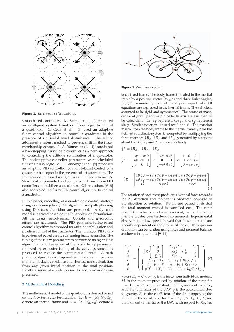
Figure 1. Basic motion of a quadrotor.

vision-based controllers. M. Santos et al. [2] proposedan intelligent system based on fuzzy logic to controla quadrotor. C. Coza et al. [3] used an adaptivefuzzy control algorithm to control a quadrotor in thepresence of sinusoidal wind disturbance. The authoraddressed a robust method to prevent drift in the fuzzymembership centres. Y. A. Younes et al. [4] introduceda backstepping fuzzy logic controller as a new approachto controlling the attitude stabilization of a quadrotor.The backstepping controller parameters were scheduledutilizing fuzzy logic. M. H. Amoozgar et al. [5] proposedan adaptive PID controller for fault-tolerant control of aquadrotor helicopter in the presence of actuator faults. ThePID gains were tuned using a fuzzy interface scheme. A.Sharma et al. presented and compared PID and fuzzy PIDcontrollers to stabilize a quadrotor. Other authors [6–8]also addressed the fuzzy PID control algorithm to controla quadrotor.

In this paper, modelling of a quadrotor, a control strategyusing a self-tuning fuzzy PID algorithm and path planningusing Dijkstra’s algorithm are presented. A dynamicmodel is derived based on the Euler-Newton formulation.All the drags, aerodynamic, Coriolis and gyroscopiceffects are neglected. The PID gain scheduling-basedcontrol algorithm is proposed for attitude stabilization andposition control of the quadrotor. The tuning of PID gainsis performed based on the self-tuning fuzzy controller. Thetuning of the fuzzy parameters is performed using an EKFalgorithm. Smart selection of the active fuzzy parameterfollowed by exclusive tuning of the active parameter isproposed to reduce the computational time. A pathplanning algorithm is proposed with two main objectivesin mind: obstacle avoidance and shortest route calculationfrom any given initial position to the final position.Finally, a series of simulation results and conclusions arepresented.

2. Mathematical Modelling

The mathematical model of the quadrotor is derived basedon the Newton-Euler formulation. Let E = {XE, YE, ZE}denote an inertial frame and B = {XB, YB, ZB} denote a

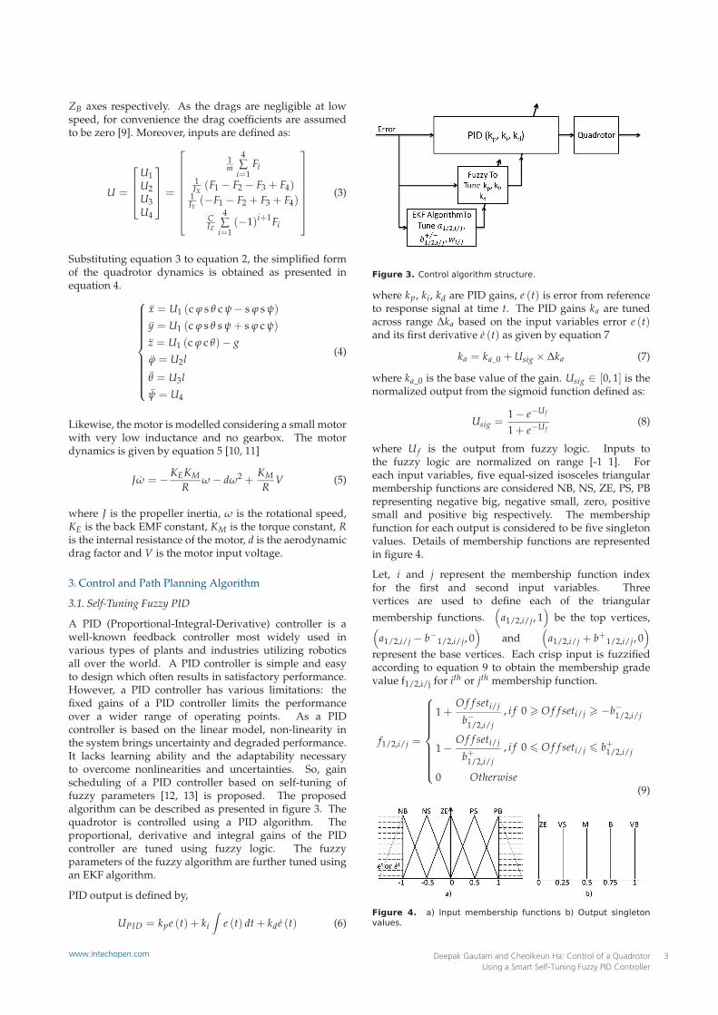
Figure 2. Coordinate system.

body fixed frame. The body frame is related to the inertialframe by a position vector (x, y, z) and three Euler angles,(ϕ, θ, ψ) representing roll, pitch and yaw respectively. Allequations are expressed in the inertial frame. The vehicle isassumed to be rigid and symmetrical. The centre of mass,centre of gravity and origin of body axis are assumed tobe coincident. Let cϕ represent cos ϕ, and sϕ representsin ϕ. Similar notation is used for θ and ψ. The rotationmatrix from the body frame to the inertial frame E

BR for thedefined coordinate system is computed by multiplying thethree matrices E

BRX , EBRY and E

BRX generated by rotationsabout the XB, YB and ZB axes respectively.EBR = E

BRZ × EBRY × E

BRX

EBR =

cψ −sψ 0sψ cψ 00 0 1

×

cθ 0 sθ0 1 0

−sθ 0 cθ

×

1 0 00 cϕ sϕ0 −sϕ cϕ

EBR =

c θ c ψ − s ϕ s θ c ψ − c ϕ s ψ c ϕ s θ c ψ − s ϕ s ψc θ s ψ − s ϕ s θ s ψ + c ϕ c ψ c ϕ s θ s ψ + s ϕ c ψ− s θ − s ϕ c θ c ϕcθ

(1)

The rotation of each rotor produces a vertical force towardsthe ZB direction and moment is produced opposite tothe direction of rotation. Rotors are paired such thatthe total moment created is cancelled out. The rotorpair 2-4 produces clockwise moment, while the rotorpair 1-3 creates counterclockwise moment. Experimentalobservation at low speed showed that these moments arelinearly dependent on the produced forces. The equationof motion can be written using force and moment balanceas shown in equation 2 [9–11]

xyzϕθψ

=

EBR

00

∑ Fi

−

K1 xK2yK3 z

1m −

00g

l (F1 − F2 − F3 + F4 + K4φ) /IXl(−F1 − F2 + F3 + F4 + K5 θ

)/IY

(CF1 − CF2 + CF3 − CF4 + K6ψ) /IZ

(2)

where Mi = C × Fi , Fi is the force from individual motors,Mi is the moment produced by rotation of the rotor fori = 1, ..., 4, C is the constant relating moment to force,m is the total mass of the UAV, g is the acceleration dueto gravity, Ki is the coefficient of the drag opposing themotion of the quadrotor, for i = 1, 2, ..., 6. IX , IY , IZ arethe moment of inertia of the UAV with respect to XB, YB,

Int. j. adv. robot. syst., 2013, Vol. 10, 380:20132 www.intechopen.com

ZB axes respectively. As the drags are negligible at lowspeed, for convenience the drag coefficients are assumedto be zero [9]. Moreover, inputs are defined as:

U =

U1U2U3U4

=

1m

4∑

i=1Fi

1IX

(F1 − F2 − F3 + F4)1IY(−F1 − F2 + F3 + F4)

CIZ

4∑

i=1(−1)i+1Fi

(3)

Substituting equation 3 to equation 2, the simplified formof the quadrotor dynamics is obtained as presented inequation 4.

x = U1 (c ϕ s θ c ψ − s ϕ s ψ)

y = U1 (c ϕ s θ s ψ + s ϕ c ψ)

z = U1 (c ϕ c θ)− gϕ = U2l

θ = U3lψ = U4

(4)

Likewise, the motor is modelled considering a small motorwith very low inductance and no gearbox. The motordynamics is given by equation 5 [10, 11]

Jω = −KEKMR

ω − dω2 +KMR

V (5)

where J is the propeller inertia, ω is the rotational speed,KE is the back EMF constant, KM is the torque constant, Ris the internal resistance of the motor, d is the aerodynamicdrag factor and V is the motor input voltage.

3. Control and Path Planning Algorithm

3.1. Self-Tuning Fuzzy PID

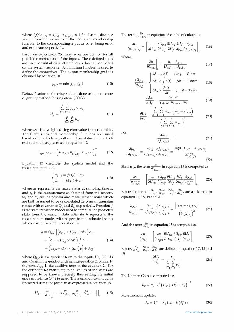
A PID (Proportional-Integral-Derivative) controller is awell-known feedback controller most widely used invarious types of plants and industries utilizing roboticsall over the world. A PID controller is simple and easyto design which often results in satisfactory performance.However, a PID controller has various limitations: thefixed gains of a PID controller limits the performanceover a wider range of operating points. As a PIDcontroller is based on the linear model, non-linearity inthe system brings uncertainty and degraded performance.It lacks learning ability and the adaptability necessaryto overcome nonlinearities and uncertainties. So, gainscheduling of a PID controller based on self-tuning offuzzy parameters [12, 13] is proposed. The proposedalgorithm can be described as presented in figure 3. Thequadrotor is controlled using a PID algorithm. Theproportional, derivative and integral gains of the PIDcontroller are tuned using fuzzy logic. The fuzzyparameters of the fuzzy algorithm are further tuned usingan EKF algorithm.

PID output is defined by,

UPID = kpe (t) + ki

∫e (t) dt + kde (t) (6)

Figure 3. Control algorithm structure.

where kp, ki, kd are PID gains, e (t) is error from referenceto response signal at time t. The PID gains ka are tunedacross range ∆ka based on the input variables error e (t)and its first derivative e (t) as given by equation 7

ka = ka_0 + Usig × ∆ka (7)

where ka_0 is the base value of the gain. Usig ∈ [0, 1] is thenormalized output from the sigmoid function defined as:

Usig =1 − e−Uf

1 + e−Uf(8)

where Uf is the output from fuzzy logic. Inputs tothe fuzzy logic are normalized on range [-1 1]. Foreach input variables, five equal-sized isosceles triangularmembership functions are considered NB, NS, ZE, PS, PBrepresenting negative big, negative small, zero, positivesmall and positive big respectively. The membershipfunction for each output is considered to be five singletonvalues. Details of membership functions are representedin figure 4.

Let, i and j represent the membership function indexfor the first and second input variables. Threevertices are used to define each of the triangular

membership functions.(

a1/2,i/j, 1)

be the top vertices,(a1/2,i/j − b−1/2,i/j, 0

)and

(a1/2,i/j + b+1/2,i/j, 0

)

represent the base vertices. Each crisp input is fuzzifiedaccording to equation 9 to obtain the membership gradevalue f1/2,i/j for ith or jth membership function.

f1/2,i/j =

1 +O f f seti/j

b−1/2,i/j

, i f 0 � O f f seti/j � −b−1/2,i/j

1 −O f f seti/j

b+1/2,i/j

, i f 0 � O f f seti/j � b+1/2,i/j

0 Otherwise(9)

Figure 4. a) Input membership functions b) Output singletonvalues.


3www.intechopen.com

where O f f seti/j = x1/2 − a1/2,i/j is defined as the distancevector from the tip vortex of the triangular membershipfunction to the corresponding input x1 or x2 being errorand error rate respectively.

Based on experience, 25 fuzzy rules are defined for allpossible combinations of the inputs. These defined rulesare used for initial calculation and are later tuned basedon the system response. A minimum function is used todefine the connectives. The output membership grade isobtained by equation 10.

µi/j = min( f1,i, f2,j) (10)

Defuzzification to the crisp value is done using the centreof gravity method for singletons (COGS).

Uf =

5∑

j=1

5∑

i=1µi,j × wi,j

5∑

j=1

5∑

i=1µi,j

(11)

where wi,j is a weighted singleton value from rule table.The fuzzy rules and membership functions are tunedbased on the EKF algorithm. The states in the EKFestimation are as presented in equation 12

x(p/i/d)k =[

a1/2,i/j b+/−1/2,i/j wi,j · · ·

]T

k(12)

Equation 13 describes the system model and themeasurement model.

{xk+1 = f (xk) + wk

zk = h(xk) + vk(13)

where xk represents the fuzzy states at sampling time k,and zk is the measurement as obtained from the sensors.wk and vk are the process and measurement noise whichare both assumed to be uncorrelated zero mean Gaussiannoises with covariance Qk and Rk respectively. Function fis the state transition model used to compute the predictedstate from the current state estimate h represents themeasurement model with respect to the estimated stateswhich is as presented in equation 14.

h = QQd

[(kp_0 + Usig × ∆kp

)e ...

+(

ki_0 + Usig × ∆ki

) ∫e...

+(

kd_0 + Usig × ∆kd

)e]+ AQd

(14)

where QQd is the quotient term to the inputs U1, U2, U3and U4 as in the quadrotor dynamics equation 2. Similarlythe term AQd is the additive term in the equation 2. Forthe extended Kalman filter, initial values of the states aresupposed to be known precisely thus setting the initialerror covariance (P−) to zero. The measurement model islinearized using the Jacobian as expressed in equation 15.

Hk =∂h∂xi

∣∣∣∣k=

[∂h

∂a1/2,i/j

∂h∂b+/−

1/2,i/j

∂h∂wi,j

· · ·]∣∣∣

k(15)

The term ∂h∂a1/2,i/j

in equation 15 can be calculated as

∂h∂a1/2,i/j

=

[∂h

∂Upid

∂Upid

∂Usig

∂Usig

∂Uf

∂Uf

∂µi,j

∂µi,j

∂a1/2,i/j

]

k

(16)

where,∂h

∂Upid

∣∣∣∣∣k

=hk − hk−1

Upidk− Upidk−1

(17)

∂Upid

∂Usig=

∆kp × e(t) f or p − Tuner

∆ki ×∫

e(t) f or i − Tuner

∆kd ×de(t)

dtf or d − Tuner

(18)

∂Usig

∂Uf=

2e−Uf

1 + 2e−Uf + e−2Uf(19)

∂Uf

∂µi,j=

5∑

m=1

5∑

n=1µm,n

(wi,j − wm,n

)

(5∑

m=1

5∑

n=1µm,n

)2 (20)

For∂µi,j

∂ f1/2,i,j= 1 (21)

∂µi,j

∂a1/2,i/j=

∂µi,j

∂ f1/2,i,j

∂ f1/2,i/j

∂a1/2,i/j=

sign[

x1/2 − a1/2,i/j

]

b−/+1/2,i/j

(22)

Similarly, the term ∂h∂b−/+

1/2,i/jin equation 15 is computed as

∂h∂b+/−

1/2,i/j

=

[∂h

∂Upid

∂Upid

∂Usig

∂Usig

∂Uf

∂Uf

∂µi,j

∂µi,j

∂b+/−1/2,i/j

]

k

(23)

where the terms ∂h∂Upid

, ∂Upid∂Usig

, ∂Usig∂Uf

, ∂Uf∂µi,j

, are as defined inequation 17, 18, 19 and 20

∂µi,j

∂b+/−1/2,i/j

=∂µi,j

∂ f1/2,i,j

∂ f1/2,i/j

∂b−/+1/2,i/j

=

∣∣∣x1/2 − a1/2,i/j

∣∣∣(

b−/+1/2,i/j

)2 (24)

And the term ∂h∂wi,j

in equation 15 is computed as

∂h∂wi,j

=

[∂h

∂Upid

∂Upid

∂Usig

∂Usig

∂Uf

∂Uf

∂wi,j

]

k

(25)

where, ∂h∂Upid

, ∂Upid∂Usig

, ∂Usig∂Uf

are defined in equation 17, 18 and19

∂Uf

∂wi,j=

µi,j5∑

i=1

5∑

j=1µi,j

(26)

The Kalman Gain is computed as:

Kk = P−k HT

k

(HkP−

k HTk + Rk

)−1(27)

Measurement updates

xk = x−k + Kk(zk − h

(x−k

))(28)


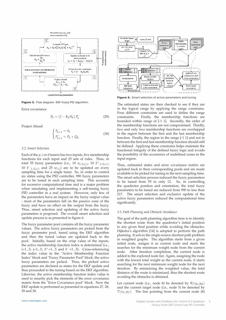
Figure 5. Flow diagram: EKF-Fuzzy-PID algorithm.

Error covariance

Pk = (I − Kk Hk) P−k (29)

Project Ahead {x−k+1 = xk

P−k+1 = Pk + Qk

(30)

3.2. Smart Selection

Each of the p, i or d tuners has two inputs, five membershipfunctions for each input and 25 sets of rules. Thus, intotal 55 fuzzy parameters (i.e., 10 a1/2,i/j, 10 b+1/2,i/j,10 b−1/2,i/j and 25 wi/j) are to be updated on everysampling time for a single tuner. So, in order to controlsix states using the PID controller, 990 fuzzy parametersare to be tuned in each sampling time. This accountsfor excessive computational time and is a major problemwhen simulating and implementing a self-tuning fuzzyPID controller in a real system. However, only few ofthe parameters have an impact on the fuzzy output value- most of the parameters fall on the passive zone of thefuzzy and have no effect on the output from the fuzzy.Thus, smart selection and updating of the active fuzzyparameters is proposed. The overall smart selection andupdate process is as presented in figure 6.

The fuzzy parameter pool contains all the fuzzy parametervalues. The active fuzzy parameters are picked from thefuzzy parameter pool, tuned using the EKF algorithmand then the tuned values are updated back to thepool. Initially, based on the crisp value of the inputs,the active membership function index is determined (i.e.,i=1...5, j=1...5, b+=1...5 and b−=1...5). Cross-referencingthe index value in the "Active Membership FunctionIndex" block and "Fuzzy Parameter Pool" block, the activefuzzy parameters are picked. Thus, the picked activeparameters are declared as states for the EKF update andthus proceeded to the tuning based on the EKF algorithm.Likewise, the active membership function index value isused to smartly pick the elements of the error covariancematrix from the "Error Covariance pool" block. Now theEKF update is performed as presented in equations 27, 28,29 and 30.

Figure 6. Smart selection of active parameters and tuning.

The estimated states are then checked to see if they arein the logical range by applying the range constrains.Four different constraints are used to define the rangeconstraints. Firstly, the membership functions arebounded within range of [-1 1]. Secondly, the order ofthe membership functions are not compromised. Thirdly,two and only two membership functions are overlappedin the region between the first and the last membershipfunction. Finally, the region in the range [-1 1] and not inbetween the first and last membership function should stillbe defined. Applying these constrains helps maintain thefunctional integrity of the defined fuzzy logic and avoidsthe possibility of the occurrence of undefined zones in theinput region.

Thus, estimated states and error covariance matrix areupdated back to their corresponding pools and are madeavailable to be picked for tuning in the next sampling time.The smart selection process reduced the fuzzy parametersto be tuned from 55 to only 12. So, in controllingthe quadrotor position and orientation, the total fuzzyparameters to be tuned are reduced from 990 to less than217. The smart selection and exclusive update of theactive fuzzy parameters reduced the computational timesignificantly.

3.3. Path Planning and Obstacle Avoidance

The goal of the path planning algorithm here is to identifythe shortest route from the quadrotor’s initial positionto any given final position while avoiding the obstacles.Dijkstra’s algorithm [14] is adopted to perform the pathplanning. It solves the single-source shortest path problemin weighted graphs. The algorithm starts from a giveninitial node, assigns it as current node and starts thesearches for the minimum weight node from the currentnode. After iteration completion, the current node isadded to the explored node list. Again, assigning the nodewith the lowest total weight as the current node, it startssearching for the next minimum weight node for the nextiteration. By minimizing the weighted value, the totaldistance of the route is minimized, thus the shortest routeavoiding the obstacles is obtained.

Let current node (i.e., node 8) be denoted by R(xR, yR)and the current target node (i.e., node 5) be denoted byT(xT , yT). The line pointing from the current node (8)


5www.intechopen.com

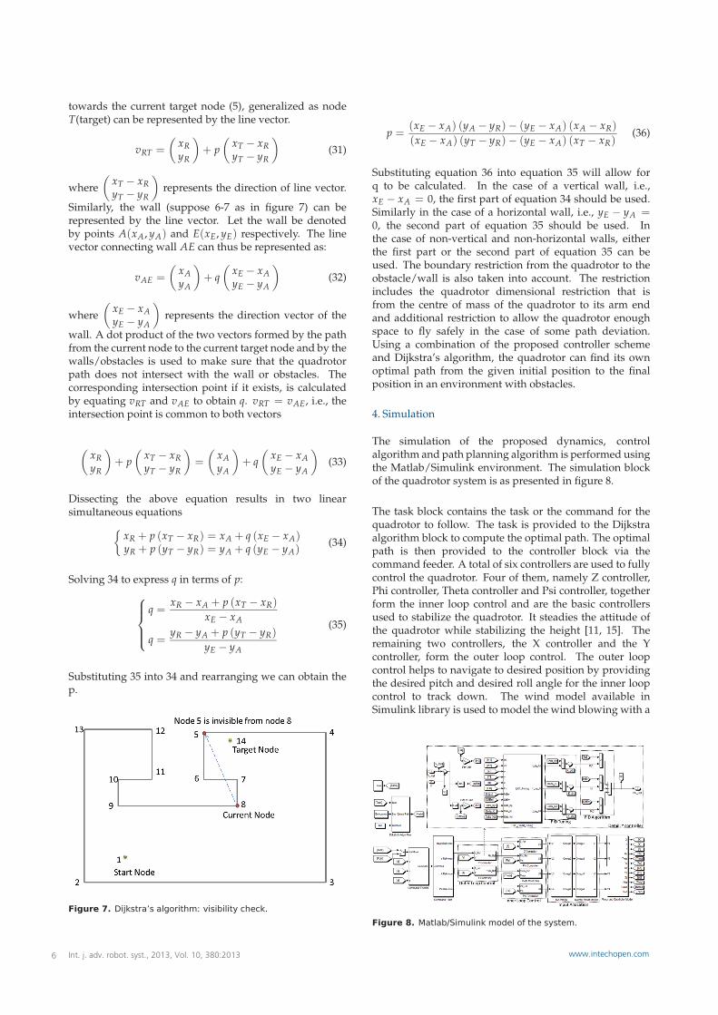
towards the current target node (5), generalized as nodeT(target) can be represented by the line vector.

vRT =

(xRyR

)+ p

(xT − xRyT − yR

)(31)

where(

xT − xRyT − yR

)represents the direction of line vector.

Similarly, the wall (suppose 6-7 as in figure 7) can berepresented by the line vector. Let the wall be denotedby points A(xA, yA) and E(xE, yE) respectively. The linevector connecting wall AE can thus be represented as:

vAE =

(xAyA

)+ q

(xE − xAyE − yA

)(32)

where(

xE − xAyE − yA

)represents the direction vector of the

wall. A dot product of the two vectors formed by the pathfrom the current node to the current target node and by thewalls/obstacles is used to make sure that the quadrotorpath does not intersect with the wall or obstacles. Thecorresponding intersection point if it exists, is calculatedby equating vRT and vAE to obtain q. vRT = vAE, i.e., theintersection point is common to both vectors

(xRyR

)+ p

(xT − xRyT − yR

)=

(xAyA

)+ q

(xE − xAyE − yA

)(33)

Dissecting the above equation results in two linearsimultaneous equations

{xR + p (xT − xR) = xA + q (xE − xA)yR + p (yT − yR) = yA + q (yE − yA)

(34)

Solving 34 to express q in terms of p:

q =xR − xA + p (xT − xR)

xE − xA

q =yR − yA + p (yT − yR)

yE − yA

(35)

Substituting 35 into 34 and rearranging we can obtain thep.

Figure 7. Dijkstra’s algorithm: visibility check.

p =(xE − xA) (yA − yR)− (yE − xA) (xA − xR)

(xE − xA) (yT − yR)− (yE − xA) (xT − xR)(36)

Substituting equation 36 into equation 35 will allow forq to be calculated. In the case of a vertical wall, i.e.,xE − xA = 0, the first part of equation 34 should be used.Similarly in the case of a horizontal wall, i.e., yE − yA =0, the second part of equation 35 should be used. Inthe case of non-vertical and non-horizontal walls, eitherthe first part or the second part of equation 35 can beused. The boundary restriction from the quadrotor to theobstacle/wall is also taken into account. The restrictionincludes the quadrotor dimensional restriction that isfrom the centre of mass of the quadrotor to its arm endand additional restriction to allow the quadrotor enoughspace to fly safely in the case of some path deviation.Using a combination of the proposed controller schemeand Dijkstra’s algorithm, the quadrotor can find its ownoptimal path from the given initial position to the finalposition in an environment with obstacles.

4. Simulation

The simulation of the proposed dynamics, controlalgorithm and path planning algorithm is performed usingthe Matlab/Simulink environment. The simulation blockof the quadrotor system is as presented in figure 8.

The task block contains the task or the command for thequadrotor to follow. The task is provided to the Dijkstraalgorithm block to compute the optimal path. The optimalpath is then provided to the controller block via thecommand feeder. A total of six controllers are used to fullycontrol the quadrotor. Four of them, namely Z controller,Phi controller, Theta controller and Psi controller, togetherform the inner loop control and are the basic controllersused to stabilize the quadrotor. It steadies the attitude ofthe quadrotor while stabilizing the height [11, 15]. Theremaining two controllers, the X controller and the Ycontroller, form the outer loop control. The outer loopcontrol helps to navigate to desired position by providingthe desired pitch and desired roll angle for the inner loopcontrol to track down. The wind model available inSimulink library is used to model the wind blowing with a

Figure 8. Matlab/Simulink model of the system.


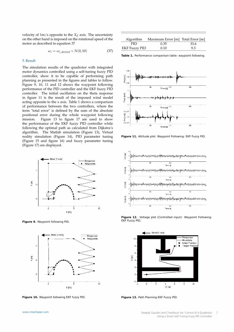
velocity of 1m/s opposite to the XE axis. The uncertaintyon the other hand is imposed on the rotational speed of themotor as described in equation 37

ωi = ωi_desired + N(0, 10) (37)

5. Result

The simulation results of the quadrotor with integratedmotor dynamics controlled using a self-tuning fuzzy PIDcontroller, show it to be capable of performing pathplanning as presented in the figures and tables to follow.Figure 9, 10, 11 and 12 shows the waypoint followingperformance of the PID controller and the EKF fuzzy PIDcontroller. The initial oscillation on the theta responsein figure 11 is the result of the imposed wind modelacting opposite to the x axis. Table 1 shows a comparisonof performance between the two controllers, where theterm "total error" is defined by the sum of the absolutepositional error during the whole waypoint followingmission. Figure 13 to figure 17 are used to showthe performance of the EKF fuzzy PID controller whilefollowing the optimal path as calculated from Dijkstra’salgorithm. The Matlab simulation (Figure 13), Virtualreality simulation (Figure 14), PID parameter tuning(Figure 15 and figure 16) and fuzzy parameter tuning(Figure 17) are displayed.

Figure 9. Waypoint following PID.

Figure 10. Waypoint following EKF fuzzy PID.

Algorithm Maximum Error [m] Total Error [m]PID 0.35 33.6

EKF Fuzzy PID 0.10 9.3

Table 1. Performance comparison table: waypoint following.

Figure 11. Attitude plot: Waypoint Following: EKF Fuzzy PID.

Figure 12. Voltage plot (Controlled input): Waypoint Following:EKF Fuzzy PID.

Figure 13. Path Planning EKF Fuzzy PID.


7www.intechopen.com

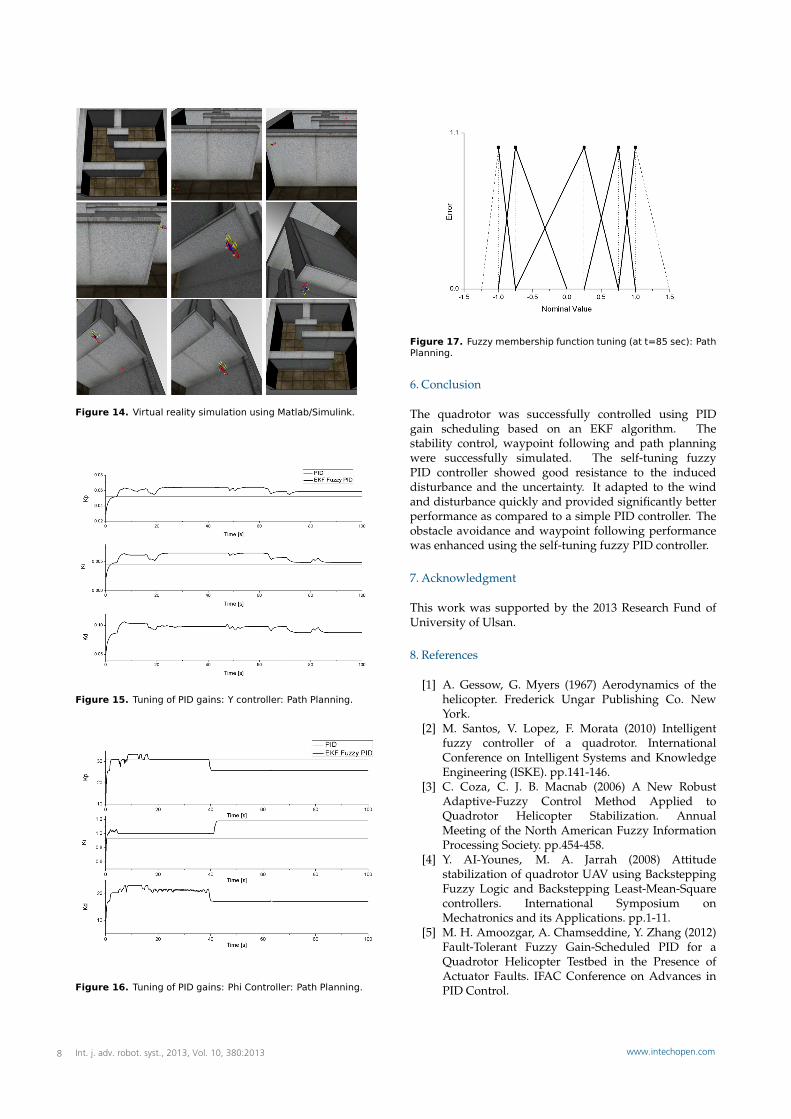
Figure 14. Virtual reality simulation using Matlab/Simulink.

Figure 15. Tuning of PID gains: Y controller: Path Planning.

Figure 16. Tuning of PID gains: Phi Controller: Path Planning.

Figure 17. Fuzzy membership function tuning (at t=85 sec): PathPlanning.

6. Conclusion

The quadrotor was successfully controlled using PIDgain scheduling based on an EKF algorithm. Thestability control, waypoint following and path planningwere successfully simulated. The self-tuning fuzzyPID controller showed good resistance to the induceddisturbance and the uncertainty. It adapted to the windand disturbance quickly and provided significantly betterperformance as compared to a simple PID controller. Theobstacle avoidance and waypoint following performancewas enhanced using the self-tuning fuzzy PID controller.

7. Acknowledgment

This work was supported by the 2013 Research Fund ofUniversity of Ulsan.

8. References

[1] A. Gessow, G. Myers (1967) Aerodynamics of thehelicopter. Frederick Ungar Publishing Co. NewYork.

[2] M. Santos, V. Lopez, F. Morata (2010) Intelligentfuzzy controller of a quadrotor. InternationalConference on Intelligent Systems and KnowledgeEngineering (ISKE). pp.141-146.

[3] C. Coza, C. J. B. Macnab (2006) A New RobustAdaptive-Fuzzy Control Method Applied toQuadrotor Helicopter Stabilization. AnnualMeeting of the North American Fuzzy InformationProcessing Society. pp.454-458.

[4] Y. AI-Younes, M. A. Jarrah (2008) Attitudestabilization of quadrotor UAV using BacksteppingFuzzy Logic and Backstepping Least-Mean-Squarecontrollers. International Symposium onMechatronics and its Applications. pp.1-11.

[5] M. H. Amoozgar, A. Chamseddine, Y. Zhang (2012)Fault-Tolerant Fuzzy Gain-Scheduled PID for aQuadrotor Helicopter Testbed in the Presence ofActuator Faults. IFAC Conference on Advances inPID Control.


[6] A. Sharma, A. Barve (2012) Controlling ofQuad-rotor UAV Using PID Controller and FuzzyLogic Controller. International Journal of Electrical,Electronics and Computer Engineering. 1(2):38-41.

[7] T. Sangyam, P. Laohapiengsak, W. Chongcharoen, I.Nilkhamhang (2012) Path Tracking of UAV UsingSelf-Tuning PID Controller Based on Fuzzy Logic.SICE Annual Conference. pp.1265-1269.

[8] G. Szafranski, R. Czyba (2011) Different Approachesof PID Control UAV Type Quadrotor. Proceedings ofInternational Micro Air Vehicles Conference. 11.

[9] E. Altug, J. P. Ostrowski, R. Mahony (2002) Controlof a Quadrotor Helicopter Using Visual Feedback.IEEE International Conference on Robotics andAutomation. 1:72-77.

[10] S. Bouabdallah, R. Siegwart (2005) Backsteppingand Sliding-mode Techniques Applied to an IndoorMicro Quadrotor. IEEE conference on Robotics andAutomation.pp.2247-2252.

[11] Tommaso Bresciani (2008) Modelling, Identificationand Control of a Quadrotor Helicopter. MasterThesis, Lund University, Lund, Sweden.

[12] K. K. Ahn, D. Q. Truong, T. Q. Thanh,B. R. Lee (2008) Online self-tuning fuzzyproportional-integral-derivative control forhydraulic load simulator. Institution of MechanicalEngineers Part I Journal of Systems and ControlEngineering. 222(12):81-96.

[13] K. K. Ahn, D. Q. Truong (2009) Online tuning fuzzyPID controller using robust extended Kalman filter.Journal of Process Control. 19(6):1011-1023.

[14] E. W. Dijkstra (1959) A note on Two problems inConnexion with Graphs. Numerische Mathematik.1:269-271.

[15] M. Orsag, M. Poropat, S. Bogdan (2010) HybridFly-by-Wire Quadrotor Control. Automatika.1:19-32.


9www.intechopen.com

Documents

Control of a Quadrotor Using a Smart Self-Tuning Fuzzy PID ...cdn.intechopen.com/pdfs/45824/InTech-Control_of_a_quadrotor_using... · International Journal of Advanced Robotic Systems