Embed Size (px)
Citation preview
6-DoF Modelling and Control of a
Remotely Operated Vehicle
by
Chu-Jou Wu, B.Eng. (Electrical)
Academic Supervisor: Assoc Prof. Karl Sammut
Engineering Discipline
College of Science and Engineering
Flinders University
July, 2018
A thesis submitted to the Flinders University in partial fulfilment of the requirements
for the degree of Master of Engineering (Electronics)
i
Abstract
Remotely Operated Vehicles (ROVs) are today commonly deployed in a range of
underwater applications, including offshore oil and gas, defence, aquaculture and scientific
research, mostly for inspection and intervention roles. In order to meet the requirements for
these roles and operate underwater effectively, the vehicles need accurate navigation and
control systems to allow the vehicle to manoeuvre and maintain station with little effort from
the operator.
This master’s thesis is concerned with two major phases: the first is modelling and system
identification of an observation class mini ROV, named BlueROV2 Heavy; and the second
is the design and development of a 6-DoF robust control system for this vehicle. Modelling
and system identification comprises mathematical modelling and the subsequent estimation
of the relevant parameters. The modelling of the BlueROV2 Heavy was carried out in 6-DoF
and consists of developing the thruster model and the dynamic model of motion of the
vehicle. A system identification approach of immersion tank testing with the use of on-board
sensors is proposed for parameter estimation where the unknown parameters are estimated
from the experimental data utilising the least squares algorithm. Due to unforeseen delays
in receiving the BlueROV2 Heavy in time, these experiments could not be performed.
Instead, the unknown parameters are currently determined by utilising the BlueROV2
Heavy’s technical specifications in combination with published data of the BlueROV.
The determined model from the system identification process was utilised to design the 6-
DoF control system for BlueROV2 Heavy in which a conventional PID controller and a
nonlinear model-based PID controller were applied, respectively. The thesis examines and
compares the performance of both controllers from results of simulations where the
nonlinear model-based control system achieves significant improvement in accuracy
especially when external disturbance is applied or when multiple movements or rotations
are required. Monte Carlo method was applied to analyse the robustness of both control
systems in consideration of random disturbances and uncertainties in the process model.
The simulation results demonstrate that the designed 6-DoF nonlinear model-based control
system is feasible to be implemented on the BlueROV2 Heavy.
ii
Declaration
I certify that this thesis does not incorporate without acknowledgment any material
previously submitted for a degree or diploma in any university; and that to the best of my
knowledge and belief it does not contain any material previously published or written by
another person except where due reference is made in the text.
iii
Acknowledgements
I would like to acknowledge my supervisor Assoc. Prof. Karl Sammut with my sincerest
gratitude for giving me this opportunity and for his invaluable guidance throughout this
research. There are no words that can sufficiently express my gratitude for his continuous
support and belief towards me. This is a treasured experience that I will carry on to my next
challenge.
I would like to thank Dr. Andrew Lammas with much appreciation for his valuable advice,
comprehensive knowledge, time and patience. His guidance and technical support provides
me direction and motivation to make this possible.
I would also like to thank Jonathan Where for his support in academic and technical and for
being willing to help in any possible way.
Finally, I would like to thank my entire family and my close friends for their support and
encouragement even without having them around during my studies.
Chu-Jou Wu
July, 2018
Adelaide
iv
Table of Contents
Abstract ........................................................................................................................................ i
Declaration .................................................................................................................................. ii
Acknowledgements ..................................................................................................................... iii
Table of Contents ....................................................................................................................... iv
List of Figures ............................................................................................................................. vi
List of Tables .............................................................................................................................. vii
Chapter 1 Introduction .................................................................................................................... 1
1.1 Background & Motivation ....................................................................................................... 1
1.2 Problem Statement ................................................................................................................ 1
1.3 Objective ............................................................................................................................... 2
1.4 Approach ............................................................................................................................... 3
1.5 Contributions and Thesis Organisation .................................................................................. 3
1.5.1 Outline of the Thesis ....................................................................................................... 3
1.5.2 Contributions ................................................................................................................... 4
Chapter 2 Literature Review ........................................................................................................... 6
2.1 ROV Classification and Related Works .................................................................................. 6
2.2 Review of Existing Control Solutions for Underwater Vehicles ............................................. 11
2.2.1 Proportional Integral Derivative (PID) Control and PID Variations ................................. 12
2.2.2 Linear Quadratic Regulator/Gaussian (LQR/LQG) ........................................................ 14
2.2.3 Sliding Mode Control (SMC) .......................................................................................... 14
2.2.4 Intelligent Control .......................................................................................................... 15
2.3 Review of Mathematical Modelling for Underwater Vehicles ................................................ 16
2.3.1 Dynamic Model ............................................................................................................. 17
2.3.2 Thruster Model .............................................................................................................. 19
2.4 Review of Parameter Estimation Methods for Underwater Vehicles .................................... 20
2.4.1 Experimental Approaches ............................................................................................. 20
2.4.2 Numerical Approaches .................................................................................................. 22
2.5 Summary ............................................................................................................................. 22
Chapter 3 Experimental Platform: BlueROV2 Heavy ..................................................................... 24
3.1 BlueROV2 Heavy Overview ................................................................................................. 24
3.2 BlueROV2 Heavy Type T200 Thrusters ............................................................................... 25
3.3 Assumptions of BlueROV2 Heavy on Dynamics .................................................................. 27
3.4 Summary ............................................................................................................................. 27
Chapter 4 Modelling of the ROV ................................................................................................... 28
4.1 Notations ............................................................................................................................. 28
4.2 Kinematic Model .................................................................................................................. 30
4.2.1 Reference Frames ........................................................................................................ 30
v
4.2.2 Transformations Between BODY and NED ................................................................... 31
4.3 Kinetic Model ....................................................................................................................... 34
4.3.1 Rigid Body Dynamics .................................................................................................... 35
4.3.2 Vehicle Hydrodynamics ................................................................................................. 36
4.3.3 Hydrostatics .................................................................................................................. 38
4.4 Thruster Model and Control Allocation ................................................................................. 39
4.5 Summary ............................................................................................................................. 42
Chapter 5 System Identification .................................................................................................... 43
5.1 System Identification Approach ........................................................................................... 43
5.1.1 The Least Squares (LS) Technique ............................................................................... 44
5.1.2 Static Experiments ........................................................................................................ 45
5.1.3 Dynamic Experiments ................................................................................................... 46
5.2 Parameter Determination ..................................................................................................... 47
5.3 Thrust Identification ............................................................................................................. 49
5.4 Summary ............................................................................................................................. 49
Chapter 6 Control of the ROV ....................................................................................................... 51
6.1 Control System Design ........................................................................................................ 52
6.1.1 Linear Conventional PID Control ................................................................................... 53
6.1.2 Nonlinear Model-based PID Control .............................................................................. 54
6.2 Control System Simulations & Result Analysis .................................................................... 56
6.2.1 Linear Conventional PID Control ................................................................................... 56
6.2.2 Nonlinear Model-based PID Control .............................................................................. 60
6.2.3 Performance Comparison of Linear Model-less and Nonlinear Model-based PID Control
Systems ................................................................................................................................. 63
6.3 Robustness Analysis of Control Systems ............................................................................ 64
6.3.1 Effect of Model Uncertainty ........................................................................................... 64
6.3.2 Effect of Current Disturbance ........................................................................................ 66
6.3.3 Effect of Model Uncertainty and Current Disturbance .................................................... 68
6.3.4 Robustness Analysis of Model-less and Model-based Control Systems ........................ 72
6.4 Summary ............................................................................................................................. 75
Chapter 7 Conclusion ................................................................................................................... 76
7.1 Summary ............................................................................................................................. 76
7.2 Conclusions ......................................................................................................................... 77
7.3 Recommendations for Future Work ..................................................................................... 79
7.3.1 Improvement of System Identification ........................................................................... 79
7.3.2 Improvement of Controller ............................................................................................. 80
7.4 Epilogue .............................................................................................................................. 81
Bibliography .............................................................................................................................. 82
vi
List of Figures
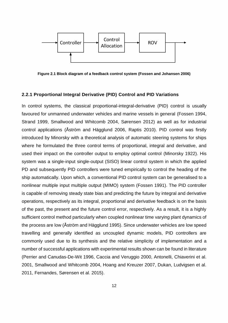
Figure 2.1 Block diagram of a feedback control system (Fossen and Johansen 2006) ................. 12
Figure 2.2 Motion in 6 DoFs (Fossen 2011) .................................................................................. 18
Figure 3.1 The BlueROV2 Heavy Configuration Retrofit Kit (BlueRobotics 2018a) ........................ 25
Figure 3.2 Diagram of hardware components on the BlueROV2 Heavy and the topside and their
connections. Communication between BlueROV2 Heavy and the topside computer is made via
Ethernet signals whereas connection between the on-board operating processing unit Raspberry Pi
3 and the autopilot Pixhawk is made through USB. ....................................................................... 25
Figure 3.3 The T200 Thruster of the BlueROV2 Heavy (BlueRobotics 2018c) .............................. 26
Figure 3.4 BlueROV2 Heavy thruster configuration from top-down view. Green and blue thrusters
indicate counter-clockwise and clockwise propellers, respectively. (BlueRobotics 2018b). ........... 26
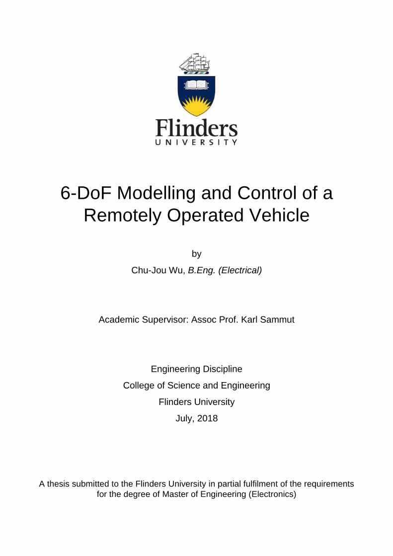
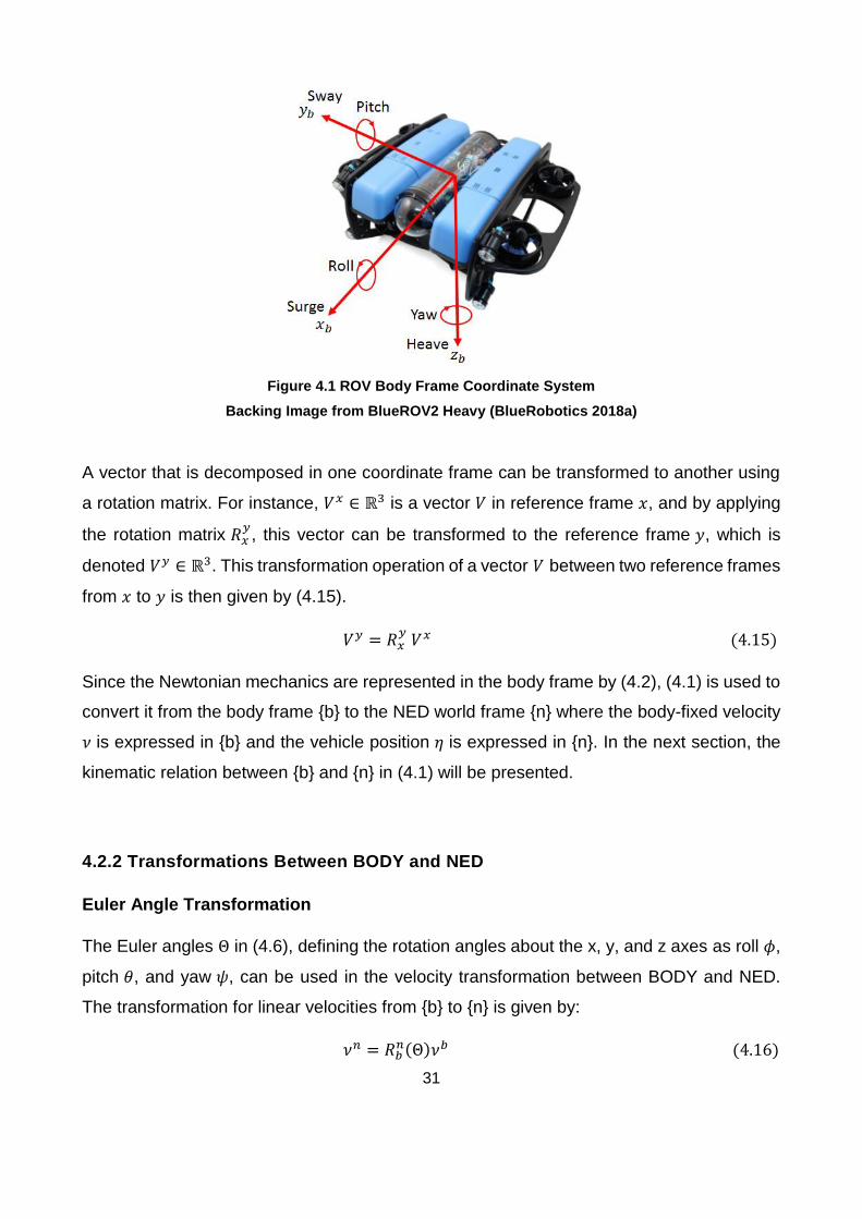
Figure 4.1 ROV Body Frame Coordinate System Backing Image from BlueROV2 Heavy
(BlueRobotics 2018a) ................................................................................................................... 31
Figure 4.2 Top view and front view of BlueROV2 Heavy thruster configuration. Backing Image from
BlueROV2 Heavy Retrofit Documentation (BlueRobotics 2018b). ................................................. 40
Figure 5.1 T200 thruster: thrust vs control input signal mapping (BlueRobotics 2018c) ................. 50
Figure 6.1 Open-loop control system block diagram (currently supported for BlueROV2 Heavy) .. 52
Figure 6.2 Feedback control system block diagram ...................................................................... 52
Figure 6.3 Linear conventional PID control system block diagram ................................................ 54
Figure 6.4 Nonlinear model-based PID control system block diagram ........................................... 56
Figure 6.5 Step responses for the position in 6 DoFs using conventional PID ............................... 58
Figure 6.6 Path following simulation results with linear PID without external disturbance .............. 59
Figure 6.7 Path following simulation results with linear PID applying current speed of 0.1 m/s on the
x and y directions .......................................................................................................................... 59
Figure 6.8 Step responses for the position in 6 DoFs using model-based PID .............................. 61
Figure 6.9 Path following simulation results with model-based PID without external disturbance .. 62
Figure 6.10 Path following simulation results with model-based PID applying current speed of 0.1
m/s on the x and y directions ........................................................................................................ 62
Figure 6.11 Comparison of step responses for 6 DoFs based on model-less and model-based control
systems using Monte Carlo simulations with model uncertainties ................................................. 65
Figure 6.12 Comparison of step responses for 6 DoFs based on model-less and model-based control
systems using Monte Carlo simulations applying water current at 0.25 m/s (within ±10% variation) in
the x, y and z directions ................................................................................................................ 67
Figure 6.13 Settling time comparison of step responses for 6 DoFs based on model-less and model-
based control systems using Monte Carlo simulations with increasing current speeds (within ±10%
variation) in the x, y and z directions ............................................................................................. 69
Figure 6.14 Steady-state error comparison of step responses for 6 DoFs based on model-less and
model-based control systems using Monte Carlo simulations with increasing current speeds (within
±10% variation) in the x, y and z directions ................................................................................... 70
Figure 6.15 Comparison of step responses for 6 DoFs based on model-less and model-based control
systems using Monte Carlo simulations in the presence of model uncertainties and current speed of
0.25 m/s with random noise in the x, y and z directions ................................................................ 71
Figure 6.16 Robustness analysis comparison of two control schemes regarding model uncertainties
..................................................................................................................................................... 73
Figure 6.17 Robustness analysis comparison of two control schemes regarding current disturbance
..................................................................................................................................................... 74
Figure 6.18 Robustness analysis comparison of two control schemes concerning both model
uncertainties and current disturbance ........................................................................................... 75
vii
List of Tables
Table 2.1 List of ROV Usage Research − 1 .................................................................................... 9
Table 2.2 List of ROV Usage Research − 2 .................................................................................. 10
Table 2.3 List of ROV Usage Research − 3 .................................................................................. 11
Table 4.1 The SNAME notation for marine vessels (SNAME 1950) .............................................. 29
Table 4.2 Moment arms of 8 thrusters of BlueROV2 Heavy .......................................................... 40
Table 5.1 A Priori information for parameters in rigid body dynamics and restoring forces ............ 48
Table 5.2 Determined added mass parameters ............................................................................ 48
Table 5.3 Determined linear and quadratic damping parameters .................................................. 48
Table 6.1 The gains used in the 6-DoF PID controller ................................................................... 56
Table 6.2 The gains used in the 6-DoF model-based PID controller ............................................. 60
Table 6.3 Performance comparison of model-less and model-based control systems ................... 63
1
CHAPTER 1
INTRODUCTION
1.1 Background & Motivation
Since there has been an increasing interest in studying, exploring and exploiting the oceans’
underwater environments in recent years, Unmanned Underwater Vehicles (UUVs) are
becoming more and more prevalent and extensively utilised in surveying, scientific, industrial
and military applications. Based on operations and shapes of the underwater vehicles, UUVs
are generally classified into two categories: Autonomous Underwater Vehicles (AUVs) and
Remotely Operated Vehicles (ROVs). An AUV can travel underwater independently for long
distances without connected cables and command inputs from operators and often has a
cylindrical shape, whereas an ROV is controlled by an operator via a tether and generally
operates at low speeds in a certain range with the design of a box shape. Due to the features
of ROVs, they have become widely used in the offshore industry for marine inspection.
Fish farming is one of the most common types of aquaculture where floating cages with
flexible nets are employed. In order to reduce the risk of fish escapes with limited operators
and costs, the development of ROV technology is invaluable for underwater operations such
as mooring and nets inspection. With the increase of the use and accessibility of ROVs to
the public for effective and safe independent operations, the demand for applying autonomy
onto ROVs has become significant for a large number of circumstances. In consideration of
autonomous operations of an ROV, the development of a control system is then crucial for
controlling the behaviour of the ROV.
1.2 Problem Statement
BlueROV2 Heavy from Blue Robotics (BlueRobotics 2018a) has been newly released in
2018 providing configuration of eight thrusters and provides the capability of full six degrees
of freedom (DoFs) control. Although BlueROV2 Heavy has a control system implemented in
its platform, it uses an open-loop controller, which can provide control abilities for manual
operation where a high level of precision is not required. Nevertheless, for autonomous
2
operations of an ROV, a robust control system is needed due to accuracy requirements and
safety of the vehicle.
The system properties for describing the behaviour of an ROV operating underwater can be
investigated using models. The development of these models is challenging and time-
consuming in both theoretical development and experimental testing. The complexity
involves highly nonlinear properties of an ROV, substantial unknown parameters in the
models, incomplete state information provided by sensors containing noisy measurements,
and system influenced by unpredictable disturbance such as currents in a coupled manner.
However, knowing system properties allows us to optimise the control design and improve
the accuracy and performance of the vehicle. Hence, this thesis will cover the modelling and
identifying BlueROV2 Heavy’s system properties as well as developing a nonlinear model-
based control algorithm based on these properties.
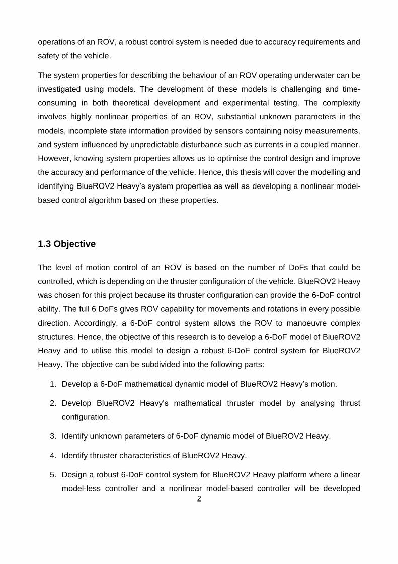
1.3 Objective
The level of motion control of an ROV is based on the number of DoFs that could be
controlled, which is depending on the thruster configuration of the vehicle. BlueROV2 Heavy
was chosen for this project because its thruster configuration can provide the 6-DoF control
ability. The full 6 DoFs gives ROV capability for movements and rotations in every possible
direction. Accordingly, a 6-DoF control system allows the ROV to manoeuvre complex
structures. Hence, the objective of this research is to develop a 6-DoF model of BlueROV2
Heavy and to utilise this model to design a robust 6-DoF control system for BlueROV2
Heavy. The objective can be subdivided into the following parts:
1. Develop a 6-DoF mathematical dynamic model of BlueROV2 Heavy’s motion.
2. Develop BlueROV2 Heavy’s mathematical thruster model by analysing thrust
configuration.
3. Identify unknown parameters of 6-DoF dynamic model of BlueROV2 Heavy.
4. Identify thruster characteristics of BlueROV2 Heavy.
5. Design a robust 6-DoF control system for BlueROV2 Heavy platform where a linear
model-less controller and a nonlinear model-based controller will be developed
3
individually and perform simulations to evaluate the performance of both control
systems.
1.4 Approach
First of all, an analytical study of theoretical models in 6 DoFs for underwater vehicles was
undertaken while a literature review was carried out to examine current knowledge and
existing solutions from previous UUV research. With the analysis of BlueROV2 Heavy’s
physical characteristics and operating speeds, several assumptions were made for the
dynamics of the vehicle in order to simplify the 6-DoF mathematical models and reduce the
number of unknown parameters in the models.
Next, a scheme of estimating parameters in the model was formulated based on the review
of system identification. This proposed approach is comprised of performing a series of
designed immersion tank experiments and then applying a suitable estimation technique to
determine unknown parameters from experimental data. However, since the BlueROV2
Heavy is currently not available for experiments, analysis of the ROV’s technical
specifications and application of parameters derived from previous BlueROV research were
applied.
Finally, since the system properties of ROVs are nonlinear, with the use of attained system
models, a nonlinear model-based controller was utilised to design a robust 6-DoF control
system for BlueROV2 Heavy while a linear controller was also designed separately. Various
predetermined experiments were operated to evaluate and compare the effectiveness and
performance of linear model-less and nonlinear model-based controllers.
1.5 Contributions and Thesis Organisation
1.5.1 Outline of the Thesis
Chapter 2 examines classification of ROVs and related research that have been done
previously; and reviews a number of control solutions that have been applied for underwater
4
vehicles as well as mathematical modelling methods and system identification approaches
for underwater vehicles.
Chapter 3 describes the BlueROV2 Heavy package and its components. The capabilities of
the vehicle and its operating system are concisely explained. The assembled BlueROV2
Heavy is shown and the assertions on dynamics about BlueROV2 Heavy that were made
are presented in this chapter
Chapter 4 presents fundamental theories and procedures of 6-DoF mathematical models
for underwater vehicles, organised by kinematic, kinetic and thruster models. The applied
assumptions based on BlueROV2 Heavy characteristics for model simplification are also
discussed.
Chapter 5 presents a system identification approach of experiment design and estimation
algorithm for determining the parameters in 6-DoF models derived in chapter 4. While the
experimental platform is not available for performing experiments, parameters determined
by analysing published technical specifications for the BlueROV2 Heavy and other available
published literature relating to the BlueROV are used instead in this chapter.
Chapter 6 concisely describes the control problem and proposes the 6-DoF nonlinear model-
based controller for the control system of BlueROV2 Heavy. The designed control system
simulations are presented and the simulation results are discussed and compared with
control system using linear model-less controller.
Chapter 7 concludes the overall results and presents suggestions for further work.
1.5.2 Contributions
To the author’s knowledge, the modelling of the BlueROV2 Heavy and the development and
analysis of the control algorithms are presented in this thesis are novel contributions. More
specifically, the following highlights the contributions made to the thesis.
1. Development of 6-DoF mathematical modelling of the BlueROV2 Heavy
2. Proposal of system identification experiments for the BlueROV2 Heavy
5
3. Determination of parameters in the 6-DoF model of the BlueROV2 Heavy by utilising
published technical specifications for the BlueROV2 Heavy and published literature
relating to the BlueROV
4. Development of a 6-DoF linear conventional PID control system and a 6-DoF
nonlinear model-based PID control system for the BlueROV2 Heavy, and
performance comparison of both algorithms by simulations
5. Robustness analysis of both control systems by applying Monte Carlo simulations
and statistical analysis
6
CHAPTER 2
LITERATURE REVIEW
This chapter presents a comprehensive literature review on existing control algorithms,
mathematical modelling methods and system identification approaches that have been
applied for underwater vehicles while ROV classification and previously developed platforms
with associated research are also examined. Accordingly, a feasible approach for
developing a robust 6-DoF control system for BlueROV2 Heavy is proposed.
2.1 ROV Classification and Related Works
ROVs can be categorised into two major classes based on the purpose of use and their
functions: observation class ROVs and work class ROVs (Capocci, Dooly et al. 2017).
Observation class ROVs are utilised for visual inspection and light intervention tasks,
whereas work class ROVs perform more serious subsea work and deep-water installations
with manipulative capability and wide power variations.
Capocci et al. presents a review of classification of ROVs in regard to size and capability,
and discusses common subsystems of the ROV. Observation class ROVs, also called
inspection ROVs, are generally small vehicles deployed in waters no deeper than a few
hundred metres and their propulsion power is limited to several kilowatts. This class of ROVs
can be subdivided into micro, mini and medium ROVs according to the size of the vehicle.
They are often fitted with thrusters, imaging devices and various types of sensors. Work
class ROVs can be divided into light and heavy work class models based on the level of
heavy duty work they are able to carry out. However, work class ROVs employ considerable
volume of equipment that leads to high overall system complexity and significant costs for
operation. Hence, when the functionalities of these large ROVs are not required, observation
class ROVs are preferred for a wide variety of applications (Capocci, Dooly et al. 2017).
Christ and Wernli provide a manual on how to use small-scale observation class ROVs for
inspection, survey and research purposes that can be applied in both scientific and industrial
7
studies (Christ and Wernli 2007). The history of ROV development and the technology
improvement of observation class ROVs were addressed in this book. It then details
necessary knowledge for the design and operations of underwater robotics and navigation
tools to attain their mission results in an efficient way. Huang discusses the degree of
autonomy for unmanned systems regarding operator controlled or program controlled by
which they might be functioned under operation modes of fully autonomous, semi-
autonomous, tele-operation and remote control depending on the levels of human
intervention (Huang 2004).
A tethered ROV can be operated with autonomy and artificial intelligence. There are three
main systems within the autonomy architecture of unmanned underwater vehicles, which
are guidance system, navigation system and control system (Fossen 2002, Fossen 2011).
The guidance system produces the desired path for the vehicle; the navigation system
determines the current state of the vehicle, such as its position, velocity and acceleration;
the control system provides command signals in controlling the vehicle in a multi-axis motion
to follow its desired trajectory. The techniques of the design of these systems are discussed
in detail in (Fossen 2002, Fossen 2011), and examples on different areas of research by the
usage of ROVs will be examined in the following.
Fernandes developed a model-based multiple input multiple output (MIMO) output feedback
motion control system along with an open-loop guidance system for an observation-class
ROV named Minerva using existing modelled parameters (Fernandes, Sørensen et al.
2015). In the guidance system, a path generation scheme was used to produce efficient
references of position, velocity and acceleration in order to guide the ROV’s motion, and a
reference model was proposed to synthesise continuous references with respect to a single
DoF motion. The applied motion control system contains dynamic positioning and trajectory
tracking capabilities such that the ROV is capable of keeping position and heading angle at
a depth of 70 m by controlling 4 DoFs of surge, sway heave and yaw of the ROV under the
assumption that the remaining DoFs of roll and pitch are self-stable (i.e. metacentric stability)
due to the design of the ROV. The author concluded that the use of the dynamic model
achieves a steadier motion such that steadier hydrodynamic effects and less plant
parameter variation would be induced as well as the higher overall motion accuracy could
be obtained.
8
Sandøy designed uDrone, a model-based advanced control system containing both an
observer and a controller for a mini ROV called BlueROV from Blue Robotics (Blue Robotics
2016). The controller uses the estimated states produced by the observer and evaluates
optimised corrective signals to control the vehicle. Although the BlueROV includes 6
thrusters, the system was simplified to the 4-DoF control of surge, sway, heave and yaw
motions. The author validated the design of the system by the implementation in Simulink
and interfaced with Robot Operating System (ROS) (Sandøy 2016). Aili and Ekelund also
modelled and developed a control system for BlueROV (Blue Robotics 2016) in which the
model parameters were estimated using EKF-based sensor fusion method in order to design
attitude, angular velocity and depth controllers. However, the attitude controller was not able
to achieve a stable system while using the feedback linearisation (Aili and Ekelund 2016).
Gonzalez designed and constructed an AUV named Mako, including mechanical and
electrical systems (Gonzalez 2004). The system identification of Mako and the simulation of
a control system were carried out for 4 DoFs of surge, heave, pitch and yaw motion control.
Lapierre et al. proposed a nonlinear path following control system using Lypaunov theory
and backstepping techniques and the simulation was performed for an underactuated AUV
with the simplified dynamic model along a desired path (Lapierre, Soetanto et al. 2003).
Image capturing is another main capability for ROVs. Jakobsen developed a software
system for a micro ROV to inspect fish cage net integrity by analysing the video feed from
the ROV. The algorithm processes and analyses camera sensor data in real-time, with the
objective of generating control signals for the ROV to move in a pattern for the investigation
of the whole cage net. Although this was not achieved as a result of the lack of sway motion
ability of the ROV, it has proven the use of an autonomous ROV for aquaculture monitoring
applications (Jakobsen 2011). In oceanography research, there are application examples in
detecting and tracking underwater objects (Walther, Edgington et al. 2004), underwater
environment mapping and reconstruction (Singh, Roman et al. 2007, Sedlazeck, Koser et
al. 2009, Marsh, Copley et al. 2013). Table 2.1 to Table 2.3 lists a number of previously
developed platforms and associated research.
9
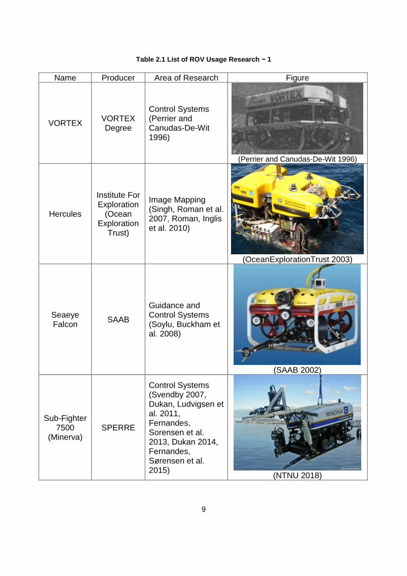
Table 2.1 List of ROV Usage Research − 1
Name Producer Area of Research Figure
VORTEX VORTEX Degree
Control Systems (Perrier and Canudas-De-Wit 1996)
(Perrier and Canudas-De-Wit 1996)
Hercules
Institute For Exploration
(Ocean Exploration
Trust)
Image Mapping (Singh, Roman et al. 2007, Roman, Inglis et al. 2010)
(OceanExplorationTrust 2003)
Seaeye Falcon
SAAB
Guidance and Control Systems (Soylu, Buckham et al. 2008)
(SAAB 2002)
Sub-Fighter 7500
(Minerva) SPERRE
Control Systems (Svendby 2007, Dukan, Ludvigsen et al. 2011, Fernandes, Sorensen et al. 2013, Dukan 2014, Fernandes, Sørensen et al. 2015)
(NTNU 2018)
10
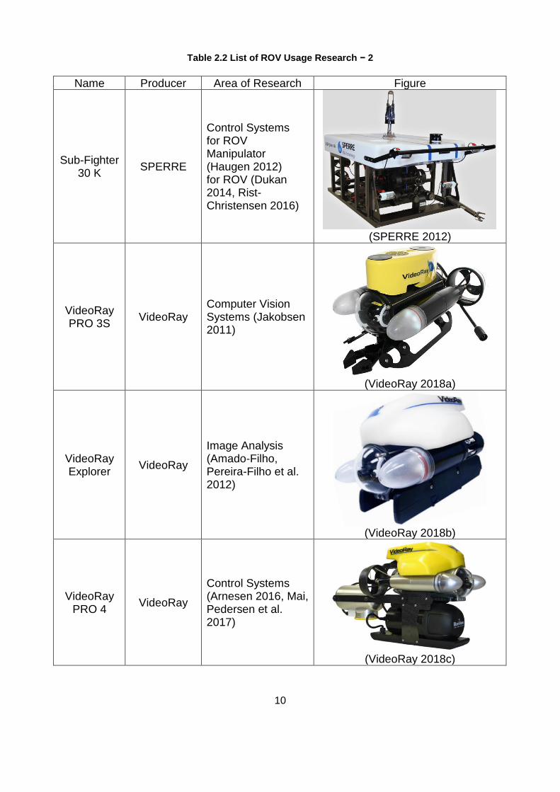
Table 2.2 List of ROV Usage Research − 2
Name Producer Area of Research Figure
Sub-Fighter 30 K
SPERRE
Control Systems for ROV Manipulator (Haugen 2012) for ROV (Dukan 2014, Rist-Christensen 2016)
(SPERRE 2012)
VideoRay PRO 3S
VideoRay Computer Vision Systems (Jakobsen 2011)
(VideoRay 2018a)
VideoRay Explorer
VideoRay
Image Analysis (Amado-Filho, Pereira-Filho et al. 2012)
(VideoRay 2018b)
VideoRay PRO 4
VideoRay
Control Systems (Arnesen 2016, Mai, Pedersen et al. 2017)
(VideoRay 2018c)
11
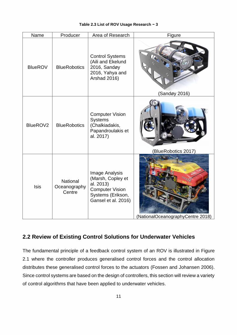
Table 2.3 List of ROV Usage Research − 3
Name Producer Area of Research Figure
BlueROV BlueRobotics
Control Systems (Aili and Ekelund 2016, Sandøy 2016, Yahya and Arshad 2016)
(Sandøy 2016)
BlueROV2 BlueRobotics
Computer Vision Systems (Chalkiadakis, Papandroulakis et al. 2017)
(BlueRobotics 2017)
Isis National
Oceanography Centre
Image Analysis (Marsh, Copley et al. 2013) Computer Vision Systems (Erikson, Gansel et al. 2016)
(NationalOceanographyCentre 2018)
2.2 Review of Existing Control Solutions for Underwater Vehicles
The fundamental principle of a feedback control system of an ROV is illustrated in Figure
2.1 where the controller produces generalised control forces and the control allocation
distributes these generalised control forces to the actuators (Fossen and Johansen 2006).
Since control systems are based on the design of controllers, this section will review a variety
of control algorithms that have been applied to underwater vehicles.
12
ControllerControl
AllocationROV
Figure 2.1 Block diagram of a feedback control system (Fossen and Johansen 2006)
2.2.1 Proportional Integral Derivative (PID) Control and PID Variations
In control systems, the classical proportional-integral-derivative (PID) control is usually
favoured for unmanned underwater vehicles and marine vessels in general (Fossen 1994,
Strand 1999, Smallwood and Whitcomb 2004, Sørensen 2012) as well as for industrial
control applications (Åström and Hägglund 2006, Raptis 2010). PID control was firstly
introduced by Minorsky with a theoretical analysis of automatic steering systems for ships
where he formulated the three control terms of proportional, integral and derivative, and
used their impact on the controller output to employ optimal control (Minorsky 1922). His
system was a single-input single-output (SISO) linear control system in which the applied
PD and subsequently PID controllers were tuned empirically to control the heading of the
ship automatically. Upon which, a conventional PID control system can be generalised to a
nonlinear multiple input multiple output (MIMO) system (Fossen 1991). The PID controller
is capable of removing steady state bias and predicting the future by integral and derivative
operations, respectively as its integral, proportional and derivative feedback is on the basis
of the past, the present and the future control error, respectively. As a result, it is a highly
sufficient control method particularly when coupled nonlinear time varying plant dynamics of
the process are low (Åström and Hägglund 1995). Since underwater vehicles are low speed
travelling and generally identified as uncoupled dynamic models, PID controllers are
commonly used due to its synthesis and the relative simplicity of implementation and a
number of successful applications with experimental results shown can be found in literature
(Perrier and Canudas-De-Wit 1996, Caccia and Veruggio 2000, Antonelli, Chiaverini et al.
2001, Smallwood and Whitcomb 2004, Hoang and Kreuzer 2007, Dukan, Ludvigsen et al.
2011, Fernandes, Sørensen et al. 2015).
13
The first dynamic positioning system was implemented by the use of traditional PID
controllers in cascade for surge, sway and yaw motions in combination with notch filters to
restrain the effects of wave forces under the assumption that the interactions are negligible
(Sargent and Cowgill 1976). However, the integral action of the controller could not be
sufficient due to couplings between motions of surge, sway and yaw. Furthermore, the
introduction of motion measurements notch filtering results in the phase lag in the control
loops.
In several applications, the conventional PID controller has its performance limitations.
When PID controllers are used alone, the exact trajectory tracking of nonlinear time varying
dynamics cannot be achieved. Moreover, PID controllers are unable to dynamically
compensate for unmodelled hydrodynamic forces of the vehicle. Yet by incorporating other
techniques into the PID design it is possible to circumvent these limitations. The nonlinear
model-based exact linearisation can be obtained either applying state feedback of the
robotics computed torque control technique (Franklin, Powell et al. 1994, Silpa-Anan,
Abdallah et al. 2000, Gonzalez 2004) or using reference feedforward terms (Smallwood and
Whitcomb 2004, Fernandes, Sørensen et al. 2015) to exactly linearise the plant dynamics.
Alternatively, since the process dynamics varies, two approaches have been suggested to
automatically alter the gains of the PID controller with regard to adapting the corresponding
variations in the dynamic properties to the process. The first method called gain scheduling
updates the controller gains discretely based on measurable disturbance inputs (Caccia and
Veruggio 2000, Sørensen 2012). The other approach of continuous adaptation (or self-
adaptation) tunes the system continuously on the basis of a measurement of its closed-loop
performance. While Hsu implemented the dynamic positioning system using PI and model-
based adaptive controller on an ROV (Hsu, Costa et al. 2000), employing an nonlinear
adaptive PD controller in the dynamic positioning for AUVs (Sun and Cheah 2003) and
ROVs (Hoang and Kreuzer 2007) has been proposed. Antonelli developed a 6-DoF adaptive
control algorithm for AUVs in the unknown dynamic parameters and time varying underwater
environments validated by sufficient experimental results (Antonelli, Chiaverini et al. 2001).
Perrier and Canudas-De-Wit designed a nonlinear robust control system using a PID
controller with an additional nonlinear loop, and performed experiments on the VORTEX
ROV (Perrier and Canudas-De-Wit 1996) while Alvarez et al presented the control of an
AUV using a robust PID controller to undertake oceanographic sampling tasks (Alvarez,
14
Caffaz et al. 2009). More applications of the nonlinear robust adaptive control strategy for
UUVs can be found in literature (Yuh 1990, Do, Pan et al. 2004, Li, Yang et al. 2012).
2.2.2 Linear Quadratic Regulator/Gaussian (LQR/LQG)
Another optimal control technique of model linearisation called linear quadratic regulator
(LQR) operates a dynamic system and provides an automated design procedure to find a
suitable state feedback controller by minimising the quadratic continuous time cost function
so as to give the best possible performance. Wahl and Gilles presented an automatic track-
keeping control system using an LQR combined with a feedforward cancellation scheme
(Wahl and Gilles 1999). Goheen and Jefferys presented a linear quadratic self-tuning
controller of linearised plant models and the performance of controlling an ROV was
examined by a nonlinear simulation (Goheen and Jefferys 1990). Arnesen developed motion
control systems to allow the Videoray Pro 4 ROV to achieve path-following in which the
heading and depth of the ROV were controlled by using a PID controller and an LQR,
respectively (Arnesen 2016). As far as the uncertainty of the system and incomplete state
information are concerned, the combination of a linear quadratic estimator (LQE) of a
Kalman filter with a LQR forms the linear quadratic Gaussian (LQG) in order for systems to
include Gaussian noise and for circumstances of that when the full state of the system might
not be directly observed. Simple LQG controllers have been applied in Juul and others (Juul,
McDermott et al. 1994, Naeem, Sutton et al. 2003, Sandøy 2016).
2.2.3 Sliding Mode Control (SMC)
Sliding mode control is a nonlinear control technique in which the dynamics of the nonlinear
system are altered by employing a discontinuous control signal to cause the system slide
along a prescribed path. Its methodology is described and derived in detail in literature (Utkin
1977, Slotine and Sastry 1983). The primary benefit of sliding mode control is that the
closed-loop response are insensitive to parameter variations and external disturbances so
as to obtain good quality of trajectory tracking and achieve robust control. Yoerger and
Slotine applied SMC in control of underwater vehicles concerning their highly nonlinear and
time varying dynamics parameters as well as model uncertainties and disturbances,
15
whereupon they presented how this method deals with nonlinearities directly to produce
robust controllers that perform predictably using a nonlinear vehicle simulations with modest
amounts of computation required (Yoerger and Slotine 1985). Haugen proposed a suitable
controller using SMC principle with the intention of forcing the manipulator of the SubFighter
30K ROV to track a desired path in the joint space, though an alternative commercial control
system was achieved by simulations that the robot was capable of following the generated
joint trajectories (Haugen 2012). More examples of control systems for underwater vehicles
based on the sliding mode approach to attain robust controllers with good simulation results
of adapting the changing dynamics and operating conditions can be found in literature
(Cristi, Papoulias et al. 1990, Healey and Lienard 1993, Gomes, Sousa et al. 2003, Soylu,
Buckham et al. 2008).
2.2.4 Intelligent Control
Intelligent control algorithm is a class of control techniques that applies a number of artificial
intelligence computing approaches to a control system that include fuzzy logic, neural
networks, Bayesian probability, machine learning, genetic algorithm and evolutionary
computation. Fuzzy logic and neural networks are the two most broadly used intelligent
control algorithms. The fuzzy logic scheme performs many-valued logic in which the
analogue input values are analysed as logical variables, and the truth values of variables
are continuous values between 0 and 1, instead of discrete levels of truth (either 1 or 0).
Raimondi and Melluso presented a closed-loop fuzzy motion control system on the basis of
Lyapunov’s stability for an under-actuated ROV where the controller ensures robustness in
relation to uncertainties caused by deep sea environment and saturation of the control
signals and an Kalman filter was implemented to compensate measurement noises
(Raimondi and Melluso 2010). Neural network controllers involve two stages of system
identification and control where a neural network model of the plant is trained in the system
identification stage for the control design. An adaptive neural network approach was applied
in (Chu, Zhu et al. 2017) for an ROV trajectory tracking control system. Furthermore, several
studies have proposed the combined use of fuzzy logic and neural network control
techniques for underwater vehicles with numerical simulations (Mills and Harris 1995, Wang
and Lee 2003). Although intelligent control algorithms contain considerable uncertainty and
16
can provide a control solution when the vehicle’s dynamics are not well known, the
implementation of the controllers consist of their own mathematical complexity and require
extensive computational resources as well as lengthy tuning processes.
Recently, combinations of the various control solutions discussed above have been
commonly used in the control of underwater vehicles such as sliding mode fuzzy controllers
for an AUV (Song and Smith 2000), adaptive fuzzy sliding mode controller for ROVs
(Sebastián and Sotelo 2007, Bessa, Dutra et al. 2010), and an adaptive neuro-fuzzy sliding
mode based on genetic algorithm control system for an ROV (Javadi-Moghaddam and
Bagheri 2010). The integration of different control schemes offers the benefits of combining
each controller’s useful properties in order to increase robustness and fault tolerance of the
overall control system.
2.3 Review of Mathematical Modelling for Underwater Vehicles
It is vital to investigate the physical properties of the model of the underwater vehicle for
control system design for a number of purposes. Since underwater vehicles might operate
under various operating conditions and they are highly complex mechatronic devices,
nonlinearities due to hydrodynamic forces and kinematics of the vehicle are considerable.
Hence, investigating and modelling these nonlinear influences is significant to the
performance and robustness of the ROV control system. Besides, the technique of nonlinear
control design offers the opportunity to directly compensate the model’s nonlinear dynamics.
Furthermore, analysing the a priori information about the dynamic equations and kinematics
of the underwater vehicle provides the ability to recognise the terms in the model that can
be eliminated so as to simplify the model and allow a simpler nonlinear control design. Lastly,
structural and parametric uncertainties will be introduced when a linear approximation of a
nonlinearity is used. By identifying the nonlinearity, the structural uncertainty can be included
in the model and the parametric uncertainty can be compensated by the use of adaptive or
robust control algorithms (Fossen 1991).
In spite of some proposed neural network modelling methods (Kodogiannis, Lisboa et al.
1996, Sayyaadi and Ura 1999), most published work on system identification for underwater
vehicles is based upon the dynamic equations of motion. Kalske presented a survey of
17
dynamic equations of motion for ROVs and submarine simulation (Kalske 1989). Modelling
and simulation of ROVs have been analysed in the literature (Lewis, Lipscombe et al. 1984).
Humphrey and Watkinson addressed the nonlinear and linear equations of motion of the
AUV UNH-EAVE (Humphreys and Watkinson 1982) while Fossen and Sagatun described
the nonlinear motion dynamics of the ROV in detail (Fossen 1991).
The motions of a marine craft take effects in 6 DoFs, which are the set of independent
movements along three directions defined as surge, sway and heave; and rotations about
three axes defined as roll, pitch and yaw as illustrated in Figure 2.2. In many cases marine
crafts are under-actuated, thus reduced-order models are commonly used in motion control
systems. However, a 6-DoF model can be used when designing state-of-the-art control
systems for a fully-actuated ROV so as to achieve controllability in all DoFs.
2.3.1 Dynamic Model
Dynamic modelling can be classified into two categories: kinematics and kinetics.
Kinematics considers geometrical aspects of motion whereas kinetics investigates the
forces that cause changes of motion. A vectorial representation can be exploited to model
physical system properties of the vehicle in 6 DoFs. The use of physical system properties
is beneficial as it allows the number of coefficients required for control system design to be
reduced. It is expressed utilising reference frames of body-fixed frame and navigation frame,
hence appropriate kinematic transformations between body frame and navigation frame
needs to be obtained (Fossen 1994). The kinematic equations have been derived by the
Euler angle representation based on ship steering framework (Abkowitz 1964). Alternatively,
kinematics has also been derived and demonstrated using spacecraft systems (Kane, Likins
et al. 1983, Hughes 1986). The analysis and derivation of quaternion kinematic was
discussed in detail in Chou (Chou 1992). The more recent and detailed examination on
kinematics can be found in literature (Goldstein 1980, Egeland and Gravdahl 2002).

18
Figure 2.2 Motion in 6 DoFs (Fossen 2011)
In kinetics, the motion equations can be derived by using the Newton-Euler formulation on
the basis of Newton’s Second Law or using Euler-Lagrange equation in mechanics (Fossen
1991). Newtonian and Lagrangian mechanics have been discussed in detail in literature
extensively (Goldstein 1980, Kane, Likins et al. 1983, Hughes 1986, Meirovitch 1990,
Egeland and Gravdahl 2002). The physical properties of the system contain rigid-body and
hydrodynamic models (Berge and Fossen 2000). By using the robot model, the rigid-body
kinetics in complete 6 DoFs can be derived and represented in a vectorial form (Fossen
1994, Fossen 2011).
Two main theories of manoeuvring and seakeeping are often used to model the effect of
external forces and moments on a marine craft. In manoeuvring theory, the vessel is moving
in calm water without wave excitation and the hydrodynamic coefficients are assumed to be
frequency independent such that the nonlinear mass damper spring system contains
constant hydrodynamic coefficients whereas wave excitation is acknowledged in
seakeeping theory. Since underwater vehicles are considered to operate below the wave
affected zone, they can be modelled with constant added mass and damping coefficients
(Fossen 2011). The hydrodynamic model of the manoeuvring theory is suitable for designing
a control system based on system identification. This model can be used to compute mass,
inertia, damping, and restoring forces, and the detailed discussion on this is found in
literature (Newman , Sarpkaya and Isaacson 1981, Faltinsen 1990, Triantafyllou and Hover
2003).
19
2.3.2 Thruster Model
In order to compute optimal control inputs of the actuators of an underwater vehicle, thruster
modelling should be applied as the thruster is the lowest layer in the control loop of the
system. The desired thrust of each thruster can be determined by control allocation, which
distributes the induced control forces to the thrusters in an optimum aspect. That is, the
control allocation is the inverse of thruster model; therefore, the thruster control input signal
can be computed with the use of the thruster model and the Moore-Penrose pseudo-inverse.
The thrust configuration and thrust coefficient matrices for underwater vehicles are
examined in detail in (Fossen 2011). However, accurately modelling thrusters is challenging
in practice as thrust forces are influenced by motor model, hydrodynamic effects and
propeller mapping. Several thruster modelling schemes for mapping relationship between
the thrust and the control signal have been proposed to resolve these difficulties. While
Yoerger et al. proposed a one-state model including motor dynamics (Yoerger, Cooke et al.
1990), Healey et al. presented a two-state model containing dynamic flow effects to
represent the four quadrant behaviour of thrusters using aerofoil propeller blades lift and
drag force data to formulate thrust and torque equations (Healey, Rock et al. 1994). In
Healey’s experimental results and comparison of two models, it was concluded that the two-
state model is capable of demonstrating the thrust overshoot in transient response whereas
the one-state model is not. However, the two-state model of Healey’s is only valid when the
forward speed of the underwater vehicle is around zero. Whitcomb and Yoerger compared
both previous models by performing experimental verifications (Whitcomb and Yoerger
1999) and additionally suggested two new model-based thrust control algorithms, yet high-
bandwidth fluid flow velocity sensors and highly accurate plant model parameters are
required. In order for the model to match with experimental results better, instead of previous
offline paradigm of thruster modelling, Bachmayer et al. proposed an online adaptive
thruster identification algorithm to determine lift and drag coefficients using look-up tables
(Bachmayer and Whitcomb 2003). Meanwhile, a three-state model with the transient effect
in the flow included was presented (Blanke, Lindegaard et al. 2000) where non-dimensional
propeller characteristics data from open water tests, thrust coefficient and advance ratio
were utilised; still the model did not show a sufficient match with experimental results for the
whole range of the advance ratio. As far as the effects of ambient flow velocity and angle
are concerned, Kim and Chung proposed a more accurate three-state thrust modelling using
20
measurable states of ambient flow velocity and propeller shaft velocity to represent the
thruster axial flow velocity (Kim and Chung 2006).
2.4 Review of Parameter Estimation Methods for Underwater Vehicles
2.4.1 Experimental Approaches
There have been a wide range of methodologies proposed to estimate the hydrodynamic
coefficients of dynamic equations of motion for unmanned underwater vehicles.
Conventional methods include tow tank experiments by using the underwater vehicle itself
(Goheen 1986) or a scale model of it (Nomoto and Hattori 1986) while measuring the forces
and moments applied to the vehicle under various operating circumstances. A routine
dynamic testing of utilising a Planar Motion Mechanism (PMM) above the towing tank was
introduced (Goodman 1960) to shift the ROV in a planar motion. Since a PMM mounted in
a towing tank can move the ROV in multiple directions by rotating the ROV, it allows a
complete model identification of hydrodynamic coefficients in all 6 DoFs to be attained.
However, PMMs are fairly costly and the test procedures consume significant amount of
time.
Another approach of on-board sensor based identification uses the measured data from on-
board sensors along with information of thrust control signals to determine the most
important dynamic parameters by a set of designed simple water tests (Indiveri 1998,
Caccia, Indiveri et al. 2000, Smallwood and Whitcomb 2003). The main advantage of using
on-board sensors is that there is no external equipment required and it can be carried out
every time the vehicle setup is altered. In other words, this approach is cost effective and
highly repeatable that suits variable configuration ROVs. Nevertheless, during these
experiments, the motion of the vehicle needs to be restrained at a single DoF to identify the
simplified uncoupled model. Thus, the effectiveness of the results considerably relies on the
accuracy of the sensors and test procedures performed. Moreover, using only on-board
sensor data to identify the forces applied to the ROV by the thrusters can be challenging as
a result of the effects of thruster-hull and thruster-thruster interactions (Goheen and Jefferys
1990).
21
As a consequence, a number of on-board sensor based identification methods have been
proposed in the interest of accurate hydrodynamic parameter estimation. Since the
underwater vehicle dynamic equations of motion can be described as a set of equations that
are linear with respect to the parameters, the least squares (LS) technique is one of the
most common methods for estimation (Goheen and Jefferys 1990, Caccia, Indiveri et al.
2000, Smallwood and Whitcomb 2003, Gonzalez 2004, Ridao, Tiano et al. 2004). Caccia et
al. presented an offline identification estimating hydrodynamic coefficients by LS on the
basis of position measurements from both a compass and a digital altimeter (Caccia, Indiveri
et al. 2000) whereas Smallwood and Whitcomb proposed an online adaptive parameter
identification using LS with the data of position provided by a Sonic High Accuracy Ranging
and Positioning System (SHARPS) time-of-flight hard-wired acoustic navigation (Smallwood
and Whitcomb 2003), though a SHARPS is relatively expensive. More recently, the
employment of computer vision-based navigation systems has become a popular option for
estimating the position of the vehicle in identification (Ridao, Tiano et al. 2004, Chen, Chang
et al. 2007) as they are low-cost and able to provide accurate location data although
developing vision-based navigation algorithms can be time-consuming.
In addition, Abkowitz firstly proposed and implemented another estimation technique of
utilising Extended Kalman Filter (EKF) in finding hydrodynamic coefficients for surface
vessels (Abkowitz 1980) and an EKF-based identification application for ships was
presented by (Liu 1993) while Goheen and Jefferys suggested to optimally integrate
measurements from different sensors using EKF for underwater vehicle identification
(Goheen and Jefferys 1990) and an application for the NPS Phoenix AUV on surge motion
parameter identification based on EKF was described by (Marco and Healey 1998).
Additionally, an application of combining both LS and EKF techniques for an ROV
identification was proposed by (Alessandri, Caccia et al. 1998).
The classical free decay test applied in determining hydrodynamic coefficients has been
introduced by Morrison and Yoerger in which the ROV oscillated in the water using three
springs and the parameters in a single DoF of heave motion were identified while the position
data was measured by SHARPS (Morrison and Yoerger 1993). Ross et al. proceeded to
apply this method to a multiple DoFs of surge and sway motions of an UUV, which is
connected to four springs and the method was validated by computer simulations (Ross,
Fossen et al. 2004). However, the precise states of the vehicle are required for this method
22
and a sufficient localisation system such as SHARPS is costly. The use of pendulum is
another type of free decay experiments in which the scaled ROV model is attached to a
pendulum instead of springs and the displacement of the pendulum is measured over time
(Eng, Lau et al. 2008, Yi and Al-Qrimli 2017). The motion of the pendulum can be interpreted
by the dynamics equations to obtain the hydrodynamic parameters of the scaled model and
the corresponding values for the full scale ROV can be predicted by scale-up. Yet, the results
attained can differ widely with various initial conditions.
2.4.2 Numerical Approaches
A Numerical approach of Computational Fluid Dynamic (CFD), which solves the Navier-
Stokes equations in fluid dynamics has been used for hydrodynamic computations of
underwater vehicles in recent years (de Barros, Dantas et al. 2008). The hydrodynamic tests
such as PMM towing tank experiments can be simulated by using CFD software so as to
obtain hydrodynamic coefficients. CFD programs that have been used to determine the
hydrodynamic model of the ROV include ANSYS Fluent (Zhang, Xu et al. 2010), Wave
Analysis MIT (WAMIT) combined with the use of Computer-aided design (CAD) software
(Eng, Chin et al. 2014, Chin, Lin et al. 2017), Phoenisc (Sarkar, Sayer et al. 1997), and
Wave Analysis by Diffraction and Morison Theory (WADAM) (Eidsvik 2015). The numerical
method provides a feasible alternative when hydrodynamic test facilities and instrumentation
are not available. However, since the numerical approach of CFD is not able to capture the
highly turbulence effect, the accuracy of its analysis is limited.
2.5 Summary
The literature review has comprehensively examined the methods of system identification
and control solutions for underwater vehicles as well as related previous works on ROVs.
This shows that there are a number of options available and each algorithm has its
advantages and limitations. Therefore, these properties of these methods have been
analysed with respect to the use of BlueROV2 Heavy for inspection and intervention. In
order to attain maximum controllability for the BlueROV2 Heavy, a full 6-DoF control system
will be developed applying the following approaches:
23
• Dynamic equations of motion modelling using vectorial representation
• Static and dynamic experiments of immersion tank testing using on-board sensors for
hydrodynamic parameter estimations
• Bollard pull tests in immersion tank for thruster characteristics identification
• The least squares algorithm for determining unknown parameters from experimental
data
• 6-DoF nonlinear model-based PID controller for controlling BlueROV2 Heavy in 6 DoFs
The next chapter describes the ROV BlueROV2 Heavy applied in this project as well as
introduces its hardware, thrusters, capabilities and assumptions that can be made for the
vehicle.
24
CHAPTER 3
EXPERIMENTAL PLATFORM: BLUEROV2 HEAVY
This chapter introduces the system of the ROV used in this thesis, named BlueROV2 Heavy
(BlueRobotics 2018a). A brief introduction of the vehicle’s hardware components, thrusters
and capabilities is presented. Additionally, a list of assumptions made on the basis of
BlueROV2 Heavy’s features is presented.
3.1 BlueROV2 Heavy Overview
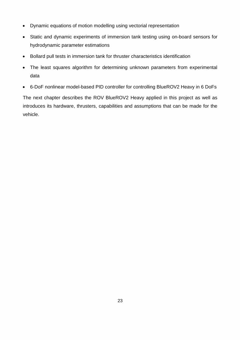
The Blue Robotics BlueROV2 Heavy, as shown in Figure 3.1, is an observation class mini
ROV that is capable of depths of 100 metres. It is an upgraded configuration of BlueROV2
and includes four horizontal and four vertical thrusters of type T200 thrusters in order to
produce 6-DoF control capacity. On the BlueROV2 Heavy, a companion computer uses a
Raspberry Pi 3 as the processing unit, which is running Ubuntu 14.04 Robot Operating
System (ROS), an open-source meta-operating system for software development of robot
applications (Quigley, Conley et al. 2009). The Raspberry Pi 3 is connected to a 3DR
Pixhawk autopilot and a live streaming HD video camera. The Pixhawk autopilot has multiple
on-board sensors including a compass, gyroscopes and accelerometers that can determine
the attitude of the vehicle. Moreover, an external water pressure sensor is also connected
to the autopilot by I2C bus for depth measurement. The autopilot collects sensor data and
sends control input signals to electronics speed controllers (ESC) for controlling thrusters
whereas the companion computer streams HD video to the surface workstation. The ROV
is self-powered by the use of an on-board battery that supports the vehicle up to 4 hours of
continuous operation.
On the surface, a topside computer is likewise running Ubuntu 14.04 ROS and a gamepad
controller is supported for manual operation. Communication between the ROV and the
topside is made via a 300 metres long neutrally buoyant CAT5 tether cable connected at
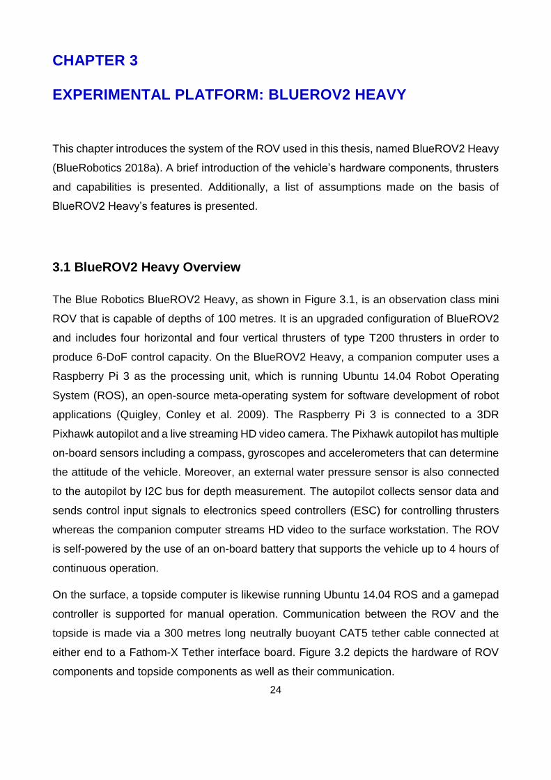
either end to a Fathom-X Tether interface board. Figure 3.2 depicts the hardware of ROV
components and topside components as well as their communication.
25
Figure 3.1 The BlueROV2 Heavy Configuration Retrofit Kit (BlueRobotics 2018a)
Raspberry Pi 3
PWMSignal Pixhawk
CameraPressure Sensor
Fathom X
Thrusters Battery
Topside Computer
Gamepad Controller
TetherESCs
Power Module
Lights
Signal35mm Connector
I2C
USB
Po
wer
Su
pp
ly
& M
on
ito
rin
g
Ethernet
BlueROV2 HeavySurface
Workstation
Fathom X
Ethernet
Figure 3.2 Diagram of hardware components on the BlueROV2 Heavy and the topside and their
connections. Communication between BlueROV2 Heavy and the topside computer is made via
Ethernet signals whereas connection between the on-board operating processing unit Raspberry Pi 3
and the autopilot Pixhawk is made through USB.
3.2 BlueROV2 Heavy Type T200 Thrusters
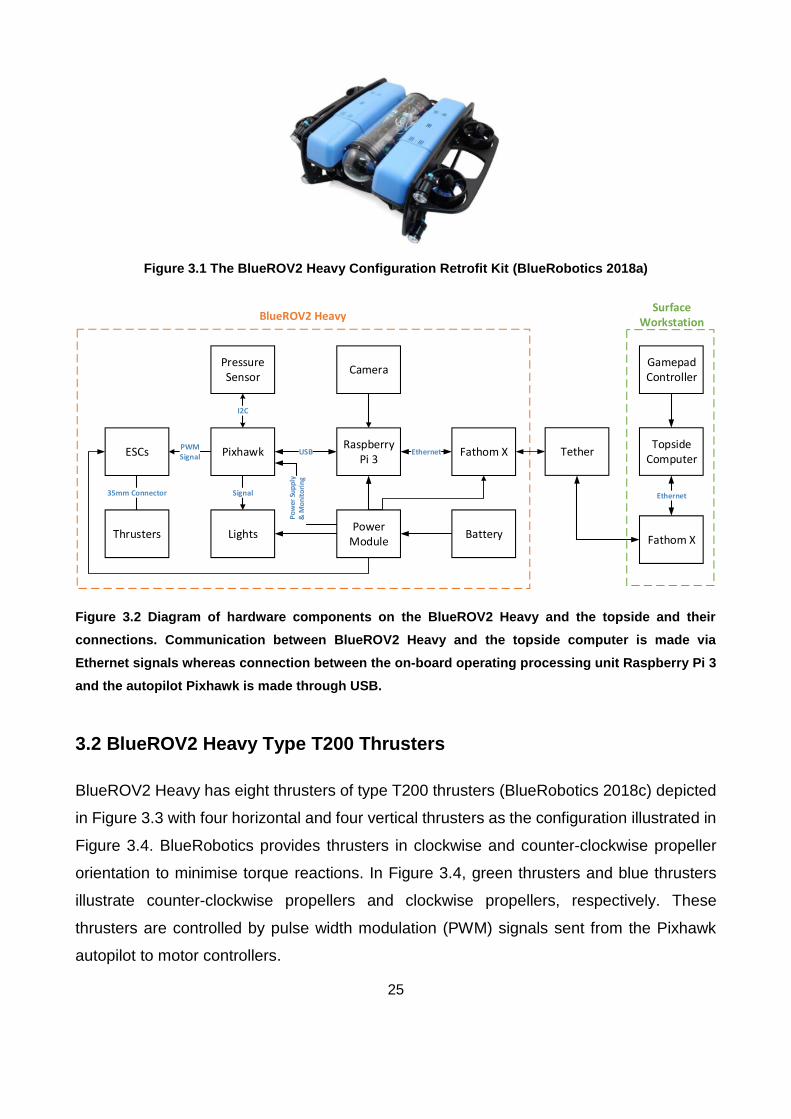
BlueROV2 Heavy has eight thrusters of type T200 thrusters (BlueRobotics 2018c) depicted
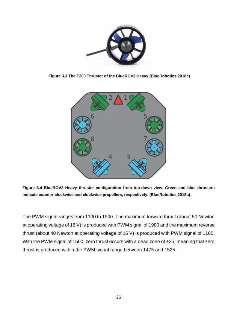
in Figure 3.3 with four horizontal and four vertical thrusters as the configuration illustrated in
Figure 3.4. BlueRobotics provides thrusters in clockwise and counter-clockwise propeller
orientation to minimise torque reactions. In Figure 3.4, green thrusters and blue thrusters
illustrate counter-clockwise propellers and clockwise propellers, respectively. These
thrusters are controlled by pulse width modulation (PWM) signals sent from the Pixhawk
autopilot to motor controllers.
26
Figure 3.3 The T200 Thruster of the BlueROV2 Heavy (BlueRobotics 2018c)
Figure 3.4 BlueROV2 Heavy thruster configuration from top-down view. Green and blue thrusters
indicate counter-clockwise and clockwise propellers, respectively. (BlueRobotics 2018b).
The PWM signal ranges from 1100 to 1900. The maximum forward thrust (about 50 Newton
at operating voltage of 16 V) is produced with PWM signal of 1900 and the maximum reverse
thrust (about 40 Newton at operating voltage of 16 V) is produced with PWM signal of 1100.
With the PWM signal of 1500, zero thrust occurs with a dead zone of ±25, meaning that zero
thrust is produced within the PWM signal range between 1475 and 1525.
27
3.3 Assumptions of BlueROV2 Heavy on Dynamics
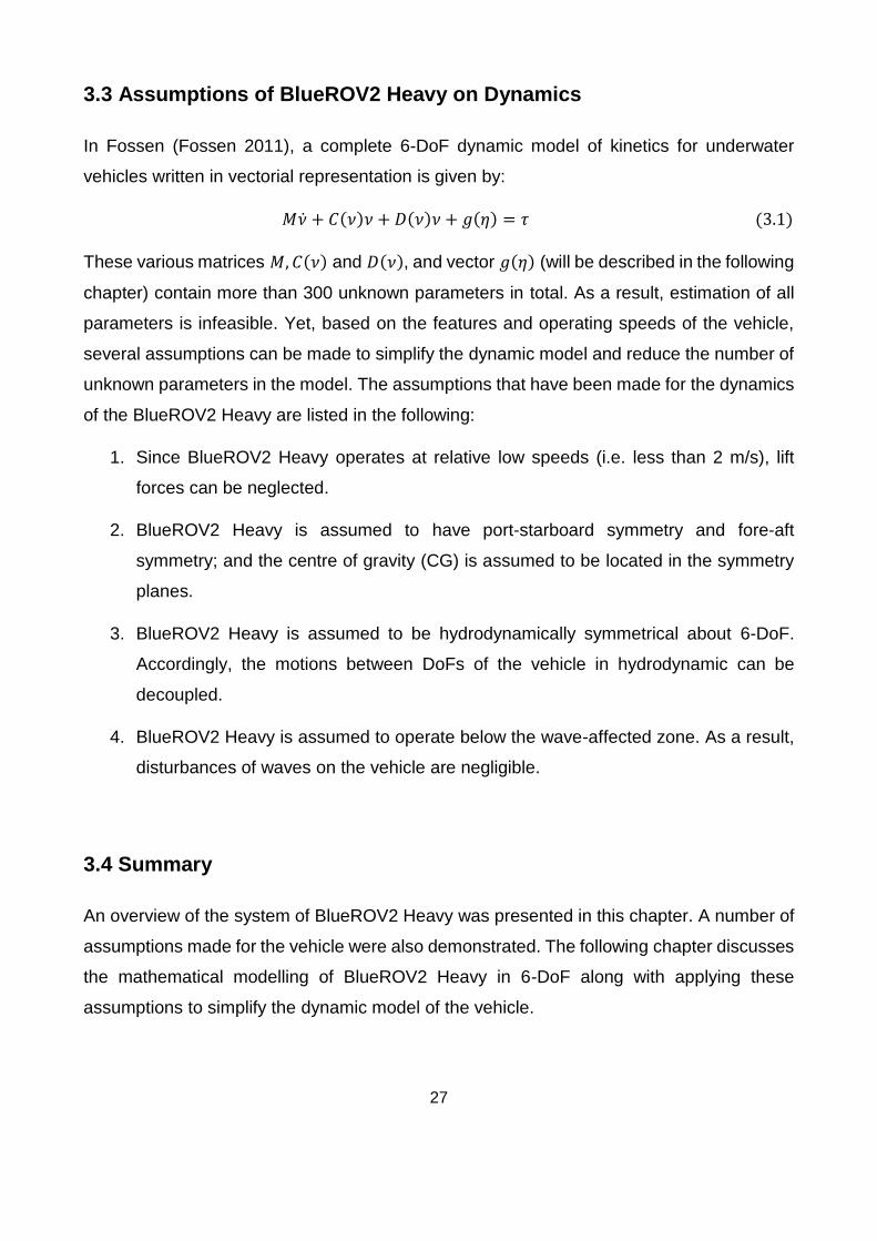
In Fossen (Fossen 2011), a complete 6-DoF dynamic model of kinetics for underwater
vehicles written in vectorial representation is given by:
𝑀�� + 𝐶(𝜈)𝜈 + 𝐷(𝜈)𝜈 + 𝑔(𝜂) = 𝜏 (3.1)
These various matrices 𝑀,𝐶(𝜈) and 𝐷(𝜈), and vector 𝑔(𝜂) (will be described in the following
chapter) contain more than 300 unknown parameters in total. As a result, estimation of all
parameters is infeasible. Yet, based on the features and operating speeds of the vehicle,
several assumptions can be made to simplify the dynamic model and reduce the number of
unknown parameters in the model. The assumptions that have been made for the dynamics
of the BlueROV2 Heavy are listed in the following:
1. Since BlueROV2 Heavy operates at relative low speeds (i.e. less than 2 m/s), lift
forces can be neglected.
2. BlueROV2 Heavy is assumed to have port-starboard symmetry and fore-aft
symmetry; and the centre of gravity (CG) is assumed to be located in the symmetry
planes.
3. BlueROV2 Heavy is assumed to be hydrodynamically symmetrical about 6-DoF.
Accordingly, the motions between DoFs of the vehicle in hydrodynamic can be
decoupled.
4. BlueROV2 Heavy is assumed to operate below the wave-affected zone. As a result,
disturbances of waves on the vehicle are negligible.
3.4 Summary
An overview of the system of BlueROV2 Heavy was presented in this chapter. A number of
assumptions made for the vehicle were also demonstrated. The following chapter discusses
the mathematical modelling of BlueROV2 Heavy in 6-DoF along with applying these
assumptions to simplify the dynamic model of the vehicle.
28
CHAPTER 4
MODELLING OF THE ROV
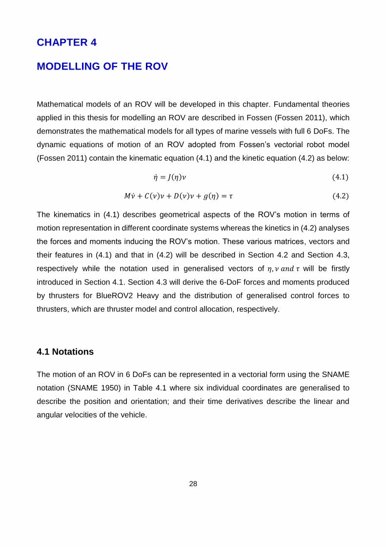
Mathematical models of an ROV will be developed in this chapter. Fundamental theories
applied in this thesis for modelling an ROV are described in Fossen (Fossen 2011), which
demonstrates the mathematical models for all types of marine vessels with full 6 DoFs. The
dynamic equations of motion of an ROV adopted from Fossen’s vectorial robot model
(Fossen 2011) contain the kinematic equation (4.1) and the kinetic equation (4.2) as below:
�� = 𝐽(𝜂)𝜈 (4.1)
𝑀�� + 𝐶(𝜈)𝜈 + 𝐷(𝜈)𝜈 + 𝑔(𝜂) = 𝜏 (4.2)
The kinematics in (4.1) describes geometrical aspects of the ROV’s motion in terms of
motion representation in different coordinate systems whereas the kinetics in (4.2) analyses
the forces and moments inducing the ROV’s motion. These various matrices, vectors and
their features in (4.1) and that in (4.2) will be described in Section 4.2 and Section 4.3,
respectively while the notation used in generalised vectors of 𝜂, 𝜈 𝑎𝑛𝑑 𝜏 will be firstly
introduced in Section 4.1. Section 4.3 will derive the 6-DoF forces and moments produced
by thrusters for BlueROV2 Heavy and the distribution of generalised control forces to
thrusters, which are thruster model and control allocation, respectively.
4.1 Notations
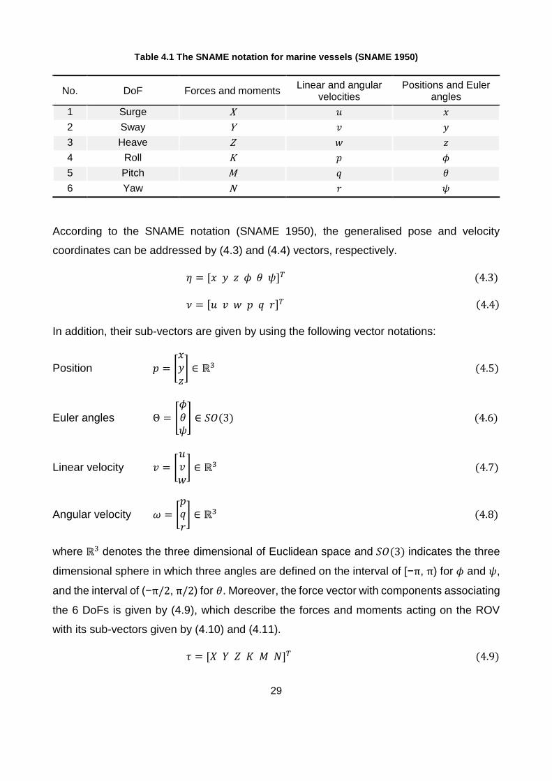
The motion of an ROV in 6 DoFs can be represented in a vectorial form using the SNAME
notation (SNAME 1950) in Table 4.1 where six individual coordinates are generalised to
describe the position and orientation; and their time derivatives describe the linear and
angular velocities of the vehicle.
29
Table 4.1 The SNAME notation for marine vessels (SNAME 1950)
No. DoF Forces and moments Linear and angular
velocities Positions and Euler
angles
1 Surge X 𝑢 𝑥
2 Sway Y 𝑣 𝑦
3 Heave Z 𝑤 𝑧
4 Roll K 𝑝 𝜙
5 Pitch M 𝑞 𝜃
6 Yaw N 𝑟 𝜓
According to the SNAME notation (SNAME 1950), the generalised pose and velocity
coordinates can be addressed by (4.3) and (4.4) vectors, respectively.
𝜂 = [𝑥 𝑦 𝑧 𝜙 𝜃 𝜓]𝑇 (4.3)
𝜈 = [𝑢 𝑣 𝑤 𝑝 𝑞 𝑟]𝑇 (4.4)
In addition, their sub-vectors are given by using the following vector notations:
Position 𝑝 = [𝑥𝑦𝑧] ∈ ℝ3 (4.5)
Euler angles Θ = [𝜙𝜃𝜓] ∈ 𝑆𝑂(3) (4.6)
Linear velocity 𝑣 = [𝑢𝑣𝑤] ∈ ℝ3 (4.7)
Angular velocity 𝜔 = [𝑝𝑞𝑟] ∈ ℝ3 (4.8)
where ℝ3 denotes the three dimensional of Euclidean space and 𝑆𝑂(3) indicates the three
dimensional sphere in which three angles are defined on the interval of [−π, π) for 𝜙 and 𝜓,
and the interval of (−π/2, π/2) for 𝜃. Moreover, the force vector with components associating
the 6 DoFs is given by (4.9), which describe the forces and moments acting on the ROV
with its sub-vectors given by (4.10) and (4.11).
𝜏 = [𝑋 𝑌 𝑍 𝐾 𝑀 𝑁]𝑇 (4.9)
30
Force on ROV 𝑓 = [𝑋𝑌𝑍] ∈ ℝ3 (4.10)
Moment on ROV 𝑚 = [𝐾𝑀𝑁] ∈ ℝ3 (4.11)
Therefore, the general motion of an ROV in 6 DoFs can be described by the following
vectors:
Position and orientation vector 𝜂 = [𝑝Θ] ∈ ℝ3 × 𝑆𝑂(3) (4.12)
Linear and angular velocity vector 𝜈 = [𝑣𝜔] ∈ ℝ6 (4.13)
Force and moment vector 𝜏 = [𝑓𝑚] ∈ ℝ6 (4.14)
4.2 Kinematic Model
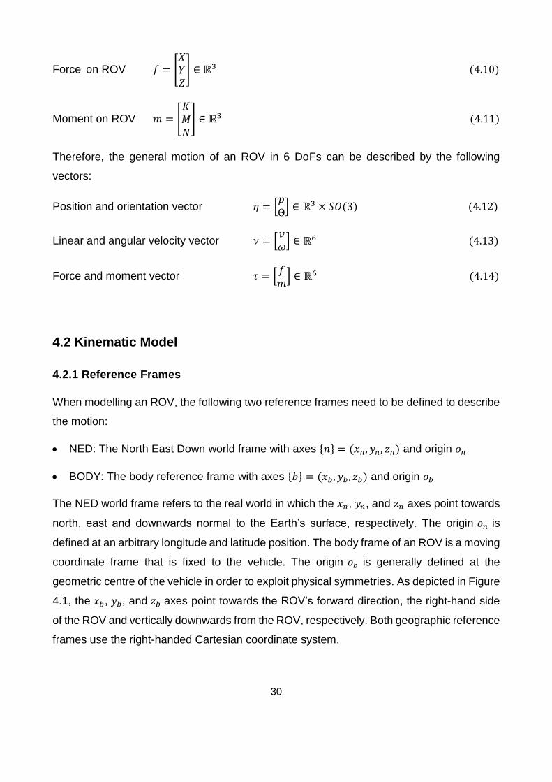
4.2.1 Reference Frames
When modelling an ROV, the following two reference frames need to be defined to describe
the motion:
• NED: The North East Down world frame with axes {𝑛} = (𝑥𝑛, 𝑦𝑛, 𝑧𝑛) and origin 𝑜𝑛
• BODY: The body reference frame with axes {𝑏} = (𝑥𝑏 , 𝑦𝑏 , 𝑧𝑏) and origin 𝑜𝑏
The NED world frame refers to the real world in which the 𝑥𝑛, 𝑦𝑛, and 𝑧𝑛 axes point towards
north, east and downwards normal to the Earth’s surface, respectively. The origin 𝑜𝑛 is
defined at an arbitrary longitude and latitude position. The body frame of an ROV is a moving
coordinate frame that is fixed to the vehicle. The origin 𝑜𝑏 is generally defined at the
geometric centre of the vehicle in order to exploit physical symmetries. As depicted in Figure
4.1, the 𝑥𝑏, 𝑦𝑏, and 𝑧𝑏 axes point towards the ROV’s forward direction, the right-hand side
of the ROV and vertically downwards from the ROV, respectively. Both geographic reference
frames use the right-handed Cartesian coordinate system.
31
Figure 4.1 ROV Body Frame Coordinate System
Backing Image from BlueROV2 Heavy (BlueRobotics 2018a)
A vector that is decomposed in one coordinate frame can be transformed to another using
a rotation matrix. For instance, 𝑉𝑥 ∈ ℝ3 is a vector 𝑉 in reference frame 𝑥, and by applying
the rotation matrix 𝑅𝑥𝑦, this vector can be transformed to the reference frame 𝑦, which is
denoted 𝑉𝑦 ∈ ℝ3. This transformation operation of a vector 𝑉 between two reference frames
from 𝑥 to 𝑦 is then given by (4.15).
𝑉𝑦 = 𝑅𝑥𝑦 𝑉𝑥 (4.15)
Since the Newtonian mechanics are represented in the body frame by (4.2), (4.1) is used to
convert it from the body frame {b} to the NED world frame {n} where the body-fixed velocity
𝜈 is expressed in {b} and the vehicle position 𝜂 is expressed in {n}. In the next section, the
kinematic relation between {b} and {n} in (4.1) will be presented.
4.2.2 Transformations Between BODY and NED
Euler Angle Transformation
The Euler angles Θ in (4.6), defining the rotation angles about the x, y, and z axes as roll 𝜙,
pitch 𝜃, and yaw 𝜓, can be used in the velocity transformation between BODY and NED.
The transformation for linear velocities from {b} to {n} is given by:
𝜈𝑛 = 𝑅𝑏𝑛(Θ)𝜈𝑏 (4.16)
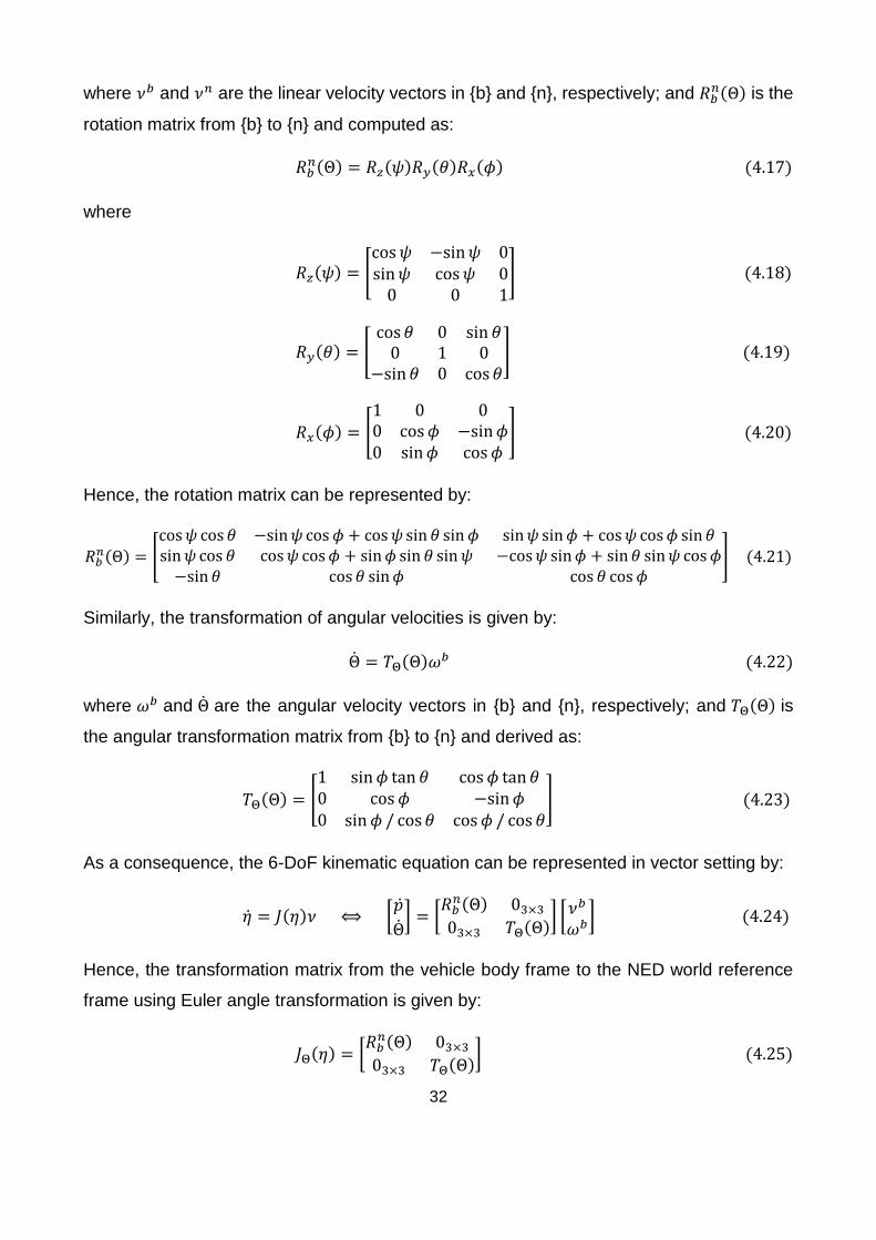
32
where 𝜈𝑏 and 𝜈𝑛 are the linear velocity vectors in {b} and {n}, respectively; and 𝑅𝑏𝑛(Θ) is the
rotation matrix from {b} to {n} and computed as:
𝑅𝑏𝑛(Θ) = 𝑅𝑧(𝜓)𝑅𝑦(𝜃)𝑅𝑥(𝜙) (4.17)
where
𝑅𝑧(𝜓) = [cos𝜓 −sin𝜓 0sin𝜓 cos𝜓 00 0 1
] (4.18)
𝑅𝑦(𝜃) = [cos 𝜃 0 sin 𝜃0 1 0
−sin 𝜃 0 cos 𝜃] (4.19)
𝑅𝑥(𝜙) = [1 0 00 cos𝜙 −sin𝜙0 sin𝜙 cos𝜙
] (4.20)
Hence, the rotation matrix can be represented by:
𝑅𝑏𝑛(Θ) = [
cos𝜓 cos 𝜃 −sin𝜓 cos𝜙 + cos𝜓 sin 𝜃 sin 𝜙 sin𝜓 sin𝜙 + cos𝜓 cos𝜙 sin 𝜃sin𝜓 cos 𝜃 cos𝜓 cos𝜙 + sin𝜙 sin 𝜃 sin𝜓 −cos𝜓 sin𝜙 + sin 𝜃 sin𝜓 cos𝜙−sin 𝜃 cos 𝜃 sin𝜙 cos 𝜃 cos 𝜙
] (4.21)
Similarly, the transformation of angular velocities is given by:
Θ = 𝑇Θ(Θ)𝜔𝑏 (4.22)
where 𝜔𝑏 and Θ are the angular velocity vectors in {b} and {n}, respectively; and 𝑇Θ(Θ) is
the angular transformation matrix from {b} to {n} and derived as:
𝑇Θ(Θ) = [
1 sin𝜙 tan 𝜃 cos𝜙 tan 𝜃0 cos𝜙 −sin𝜙0 sin 𝜙 / cos 𝜃 cos𝜙 / cos 𝜃
] (4.23)
As a consequence, the 6-DoF kinematic equation can be represented in vector setting by:
�� = 𝐽(𝜂)𝜈 ⟺ [��
Θ] = [
𝑅𝑏𝑛(Θ) 03×303×3 𝑇Θ(Θ)
] [𝜈𝑏
𝜔𝑏] (4.24)
Hence, the transformation matrix from the vehicle body frame to the NED world reference
frame using Euler angle transformation is given by:
𝐽Θ(𝜂) = [𝑅𝑏𝑛(Θ) 03×303×3 𝑇Θ(Θ)
] (4.25)
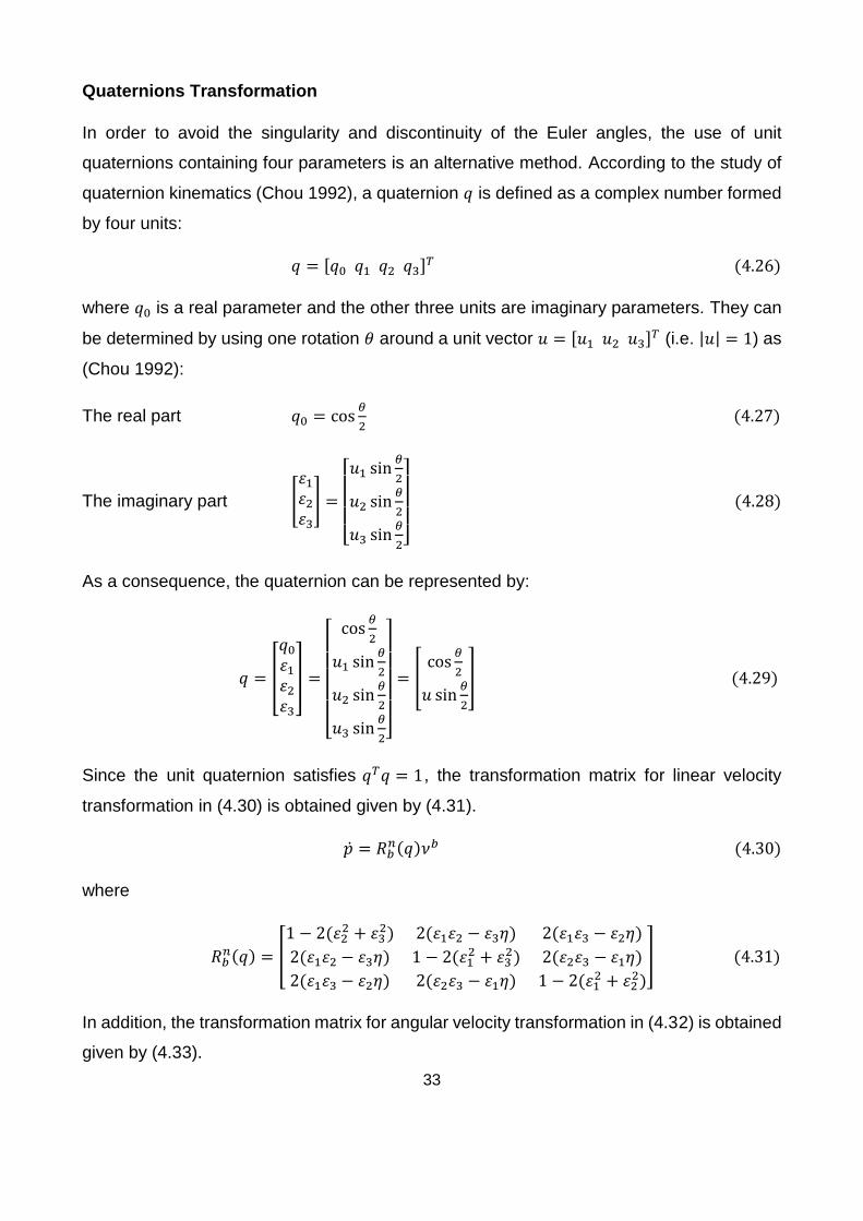
33
Quaternions Transformation
In order to avoid the singularity and discontinuity of the Euler angles, the use of unit
quaternions containing four parameters is an alternative method. According to the study of
quaternion kinematics (Chou 1992), a quaternion 𝑞 is defined as a complex number formed
by four units:
𝑞 = [𝑞0 𝑞1 𝑞2 𝑞3]𝑇 (4.26)
where 𝑞0 is a real parameter and the other three units are imaginary parameters. They can
be determined by using one rotation 𝜃 around a unit vector 𝑢 = [𝑢1 𝑢2 𝑢3]𝑇 (i.e. |𝑢| = 1) as
(Chou 1992):
The real part 𝑞0 = cos𝜃
2 (4.27)
The imaginary part [
𝜀1𝜀2𝜀3] =
[ 𝑢1 sin
𝜃
2
𝑢2 sin𝜃
2
𝑢3 sin𝜃
2]
(4.28)
As a consequence, the quaternion can be represented by:
𝑞 = [
𝑞0𝜀1𝜀2𝜀3
] =
[ cos
𝜃
2
𝑢1 sin𝜃
2
𝑢2 sin𝜃
2
𝑢3 sin𝜃
2]
= [cos
𝜃
2
𝑢 sin𝜃
2
] (4.29)
Since the unit quaternion satisfies 𝑞𝑇𝑞 = 1, the transformation matrix for linear velocity
transformation in (4.30) is obtained given by (4.31).
�� = 𝑅𝑏𝑛(𝑞)𝜈𝑏 (4.30)
where
𝑅𝑏𝑛(𝑞) = [
1 − 2(𝜀22 + 𝜀3
2) 2(𝜀1𝜀2 − 𝜀3𝜂) 2(𝜀1𝜀3 − 𝜀2𝜂)
2(𝜀1𝜀2 − 𝜀3𝜂) 1 − 2(𝜀12 + 𝜀3
2) 2(𝜀2𝜀3 − 𝜀1𝜂)
2(𝜀1𝜀3 − 𝜀2𝜂) 2(𝜀2𝜀3 − 𝜀1𝜂) 1 − 2(𝜀12 + 𝜀2
2)
] (4.31)
In addition, the transformation matrix for angular velocity transformation in (4.32) is obtained
given by (4.33).
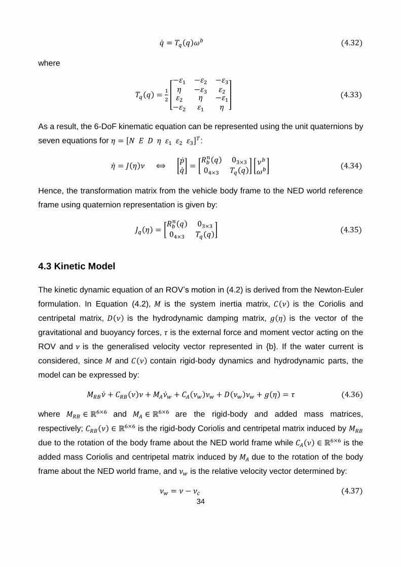
34
�� = 𝑇𝑞(𝑞)𝜔𝑏 (4.32)
where
𝑇𝑞(𝑞) =1
2[
−𝜀1 −𝜀2 −𝜀3𝜂 −𝜀3 𝜀2𝜀2−𝜀2
𝜂𝜀1
−𝜀1𝜂
] (4.33)
As a result, the 6-DoF kinematic equation can be represented using the unit quaternions by
seven equations for 𝜂 = [𝑁 𝐸 𝐷 𝜂 𝜀1 𝜀2 𝜀3]𝑇:
�� = 𝐽(𝜂)𝜈 ⟺ [����] = [
𝑅𝑏𝑛(𝑞) 03×304×3 𝑇𝑞(𝑞)
] [𝜈𝑏
𝜔𝑏] (4.34)
Hence, the transformation matrix from the vehicle body frame to the NED world reference
frame using quaternion representation is given by:
𝐽𝑞(𝜂) = [𝑅𝑏𝑛(𝑞) 03×304×3 𝑇𝑞(𝑞)
] (4.35)
4.3 Kinetic Model
The kinetic dynamic equation of an ROV’s motion in (4.2) is derived from the Newton-Euler
formulation. In Equation (4.2), 𝑀 is the system inertia matrix, 𝐶(𝜈) is the Coriolis and
centripetal matrix, 𝐷(𝜈) is the hydrodynamic damping matrix, 𝑔(𝜂) is the vector of the
gravitational and buoyancy forces, 𝜏 is the external force and moment vector acting on the
ROV and 𝜈 is the generalised velocity vector represented in {b}. If the water current is
considered, since 𝑀 and 𝐶(𝜈) contain rigid-body dynamics and hydrodynamic parts, the
model can be expressed by:
𝑀𝑅𝐵�� + 𝐶𝑅𝐵(𝜈)𝜈 + 𝑀𝐴��𝑤 + 𝐶𝐴(𝜈𝑤)𝜈𝑤 + 𝐷(𝜈𝑤)𝜈𝑤 + 𝑔(𝜂) = 𝜏 (4.36)
where 𝑀𝑅𝐵 ∈ ℝ6×6 and 𝑀𝐴 ∈ ℝ6×6 are the rigid-body and added mass matrices,
respectively; 𝐶𝑅𝐵(𝜈) ∈ ℝ6×6 is the rigid-body Coriolis and centripetal matrix induced by 𝑀𝑅𝐵
due to the rotation of the body frame about the NED world frame while 𝐶𝐴(𝜈) ∈ ℝ6×6 is the
added mass Coriolis and centripetal matrix induced by 𝑀𝐴 due to the rotation of the body
frame about the NED world frame, and 𝜈𝑤 is the relative velocity vector determined by:
𝜈𝑤 = 𝜈 − 𝜈𝑐 (4.37)
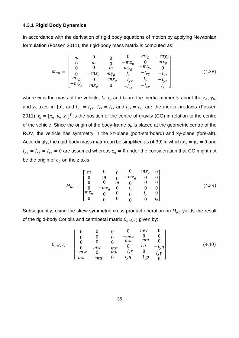
35
4.3.1 Rigid Body Dynamics
In accordance with the derivation of rigid body equations of motion by applying Newtonian
formulation (Fossen 2011), the rigid-body mass matrix is computed as:
𝑀𝑅𝐵 =
[ 𝑚
000
𝑚𝑧𝑔−𝑚𝑦𝑔
0𝑚0
−𝑚𝑧𝑔0
𝑚𝑥𝑔
00𝑚𝑚𝑦𝑔−𝑚𝑥𝑔0
0−𝑚𝑧𝑔𝑚𝑦𝑔𝐼𝑥
−𝐼𝑦𝑥−𝐼𝑧𝑥
𝑚𝑧𝑔0
−𝑚𝑥𝑔−𝐼𝑥𝑦𝐼𝑦
−𝐼𝑧𝑦
−𝑚𝑦𝑔𝑚𝑥𝑔0
−𝐼𝑥𝑧−𝐼𝑦𝑧𝐼𝑧 ]
(4.38)
where 𝑚 is the mass of the vehicle, 𝐼𝑥, 𝐼𝑦 and 𝐼𝑧 are the inertia moments about the 𝑥𝑏, 𝑦𝑏,
and 𝑧𝑏 axes in {b}, and 𝐼𝑥𝑦 = 𝐼𝑦𝑥 , 𝐼𝑥𝑧 = 𝐼𝑧𝑥 and 𝐼𝑦𝑧 = 𝐼𝑧𝑦 are the inertia products (Fossen
2011); 𝑟𝑔 = [𝑥𝑔 𝑦𝑔 𝑧𝑔]𝑇 is the position of the centre of gravity (CG) in relation to the centre
of the vehicle. Since the origin of the body-frame 𝑜𝑏 is placed at the geometric centre of the
ROV, the vehicle has symmetry in the xz-plane (port-starboard) and xy-plane (fore-aft).
Accordingly, the rigid-body mass matrix can be simplified as (4.39) in which 𝑥𝑔 = 𝑦𝑔 = 0 and
𝐼𝑥𝑦 = 𝐼𝑥𝑧 = 𝐼𝑦𝑧 = 0 are assumed whereas 𝑧𝑔 ≠ 0 under the consideration that CG might not
be the origin of 𝑜𝑏 on the z axis.
𝑀𝑅𝐵 =
[ 𝑚000
𝑚𝑧𝑔0
0𝑚0
−𝑚𝑧𝑔00
00𝑚000
0−𝑚𝑧𝑔0𝐼𝑥00
𝑚𝑧𝑔000𝐼𝑦0
00000𝐼𝑧]
(4.39)
Subsequently, using the skew-symmetric cross-product operation on 𝑀𝑅𝐵 yields the result
of the rigid-body Coriolis and centripetal matrix 𝐶𝑅𝐵(𝜈) given by:
𝐶𝑅𝐵(𝜈) =
[ 0
000
−𝑚𝑤𝑚𝑣
000
𝑚𝑤0
−𝑚𝑢
000
−𝑚𝑣−𝑚𝑢0
0−𝑚𝑤𝑚𝑣0
−𝐼𝑧𝑟𝐼𝑦𝑞
𝑚𝑤0
−𝑚𝑢𝐼𝑧𝑟0
−𝐼𝑥𝑝
000
−𝐼𝑦𝑞
𝐼𝑥𝑝0 ]
(4.40)
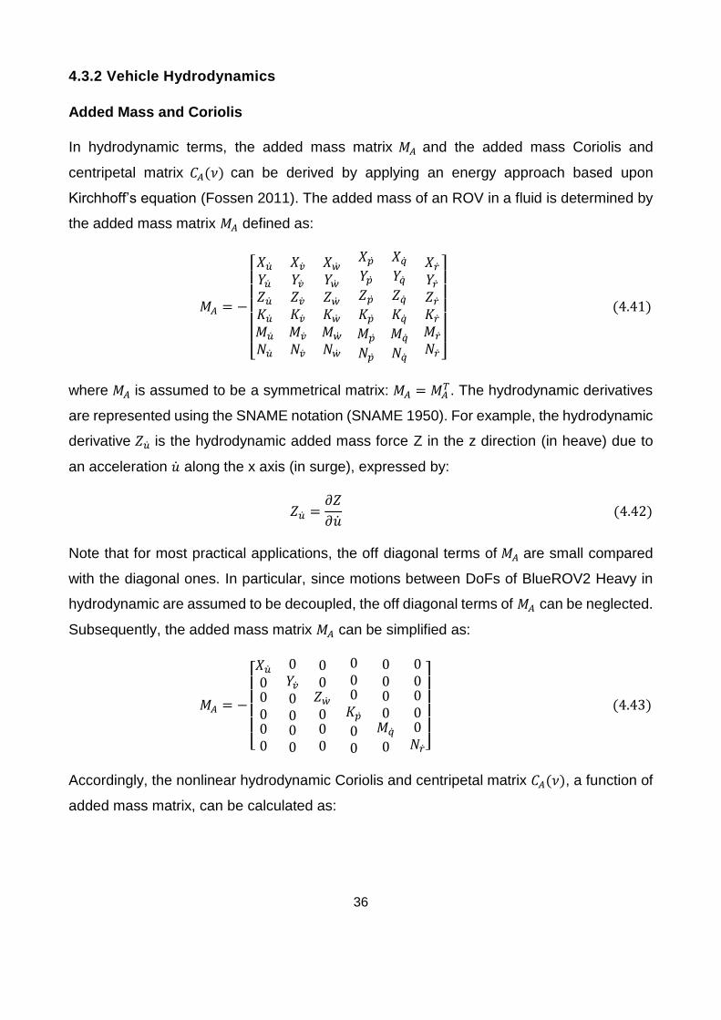
36
4.3.2 Vehicle Hydrodynamics
Added Mass and Coriolis
In hydrodynamic terms, the added mass matrix 𝑀𝐴 and the added mass Coriolis and
centripetal matrix 𝐶𝐴(𝜈) can be derived by applying an energy approach based upon
Kirchhoff’s equation (Fossen 2011). The added mass of an ROV in a fluid is determined by
the added mass matrix 𝑀𝐴 defined as:
𝑀𝐴 = −
[ 𝑋��
𝑌��𝑍��𝐾��
𝑀��
𝑁��
𝑋��
𝑌��𝑍��𝐾��
𝑀��
𝑁��
𝑋��
𝑌��𝑍��𝐾��
𝑀��
𝑁��
𝑋��
𝑌��𝑍��𝐾��
𝑀��
𝑁��
𝑋��
𝑌��𝑍��𝐾��
𝑀��
𝑁��
𝑋��
𝑌��𝑍��𝐾��
𝑀��
𝑁�� ]
(4.41)
where 𝑀𝐴 is assumed to be a symmetrical matrix: 𝑀𝐴 = 𝑀𝐴𝑇. The hydrodynamic derivatives
are represented using the SNAME notation (SNAME 1950). For example, the hydrodynamic
derivative 𝑍�� is the hydrodynamic added mass force Z in the z direction (in heave) due to
an acceleration �� along the x axis (in surge), expressed by:
𝑍�� =𝜕𝑍
𝜕�� (4.42)
Note that for most practical applications, the off diagonal terms of 𝑀𝐴 are small compared
with the diagonal ones. In particular, since motions between DoFs of BlueROV2 Heavy in
hydrodynamic are assumed to be decoupled, the off diagonal terms of 𝑀𝐴 can be neglected.
Subsequently, the added mass matrix 𝑀𝐴 can be simplified as:
𝑀𝐴 = −
[ 𝑋��
00000
0𝑌��0000
00𝑍��000
000𝐾��
00
0000𝑀��
0
00000𝑁��]
(4.43)
Accordingly, the nonlinear hydrodynamic Coriolis and centripetal matrix 𝐶𝐴(𝜈), a function of
added mass matrix, can be calculated as:
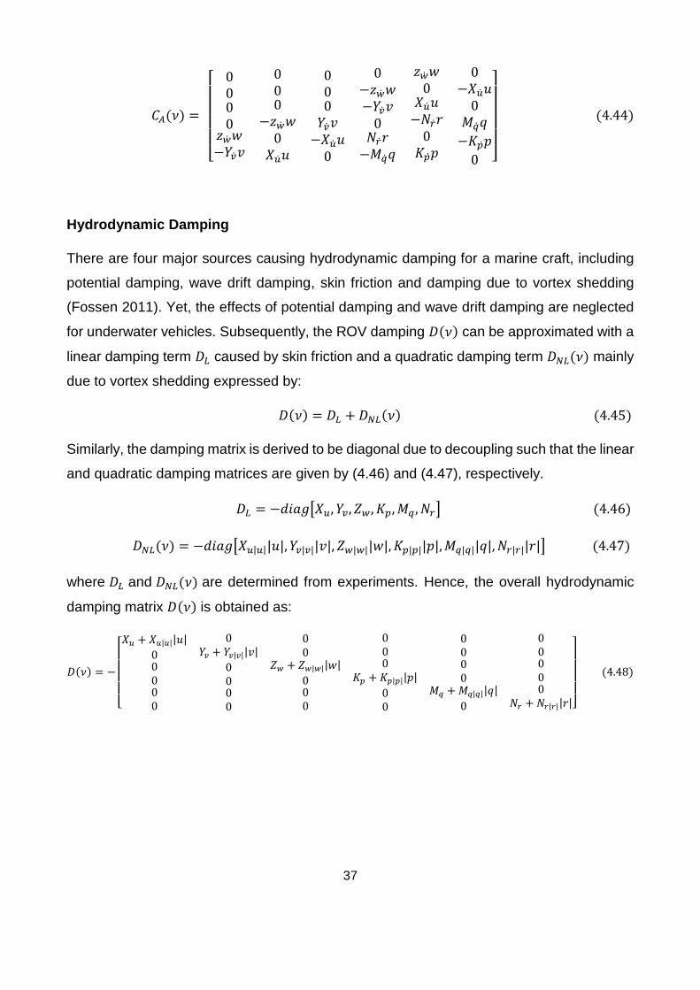
37
𝐶𝐴(𝜈) =
[ 0
000
𝑧��𝑤−𝑌��𝑣
000
−𝑧��𝑤0
𝑋��𝑢
000𝑌��𝑣−𝑋��𝑢0
0−𝑧��𝑤−𝑌��𝑣0
𝑁��𝑟−𝑀��𝑞
𝑧��𝑤0
𝑋��𝑢−𝑁��𝑟0
𝐾��𝑝
0−𝑋��𝑢0
𝑀��𝑞
−𝐾��𝑝
0 ]
(4.44)
Hydrodynamic Damping
There are four major sources causing hydrodynamic damping for a marine craft, including
potential damping, wave drift damping, skin friction and damping due to vortex shedding
(Fossen 2011). Yet, the effects of potential damping and wave drift damping are neglected
for underwater vehicles. Subsequently, the ROV damping 𝐷(𝜈) can be approximated with a
linear damping term 𝐷𝐿 caused by skin friction and a quadratic damping term 𝐷𝑁𝐿(𝜈) mainly
due to vortex shedding expressed by:
𝐷(𝜈) = 𝐷𝐿 + 𝐷𝑁𝐿(𝜈) (4.45)
Similarly, the damping matrix is derived to be diagonal due to decoupling such that the linear
and quadratic damping matrices are given by (4.46) and (4.47), respectively.
𝐷𝐿 = −𝑑𝑖𝑎𝑔[𝑋𝑢, 𝑌𝑣, 𝑍𝑤, 𝐾𝑝, 𝑀𝑞 , 𝑁𝑟] (4.46)
𝐷𝑁𝐿(𝜈) = −𝑑𝑖𝑎𝑔[𝑋𝑢|𝑢||𝑢|, 𝑌𝑣|𝑣||𝑣|, 𝑍𝑤|𝑤||𝑤|, 𝐾𝑝|𝑝||𝑝|,𝑀𝑞|𝑞||𝑞|, 𝑁𝑟|𝑟||𝑟|] (4.47)
where 𝐷𝐿 and 𝐷𝑁𝐿(𝜈) are determined from experiments. Hence, the overall hydrodynamic
damping matrix 𝐷(𝜈) is obtained as:
𝐷(𝜈) = −
[ 𝑋𝑢 + 𝑋𝑢|𝑢||𝑢|
00000
0𝑌𝑣 + 𝑌𝑣|𝑣||𝑣|
0000
00
𝑍𝑤 + 𝑍𝑤|𝑤||𝑤|
000
000
𝐾𝑝 + 𝐾𝑝|𝑝||𝑝|
00
0000
𝑀𝑞 +𝑀𝑞|𝑞||𝑞|
0
00000
𝑁𝑟 + 𝑁𝑟|𝑟||𝑟|]
(4.48)
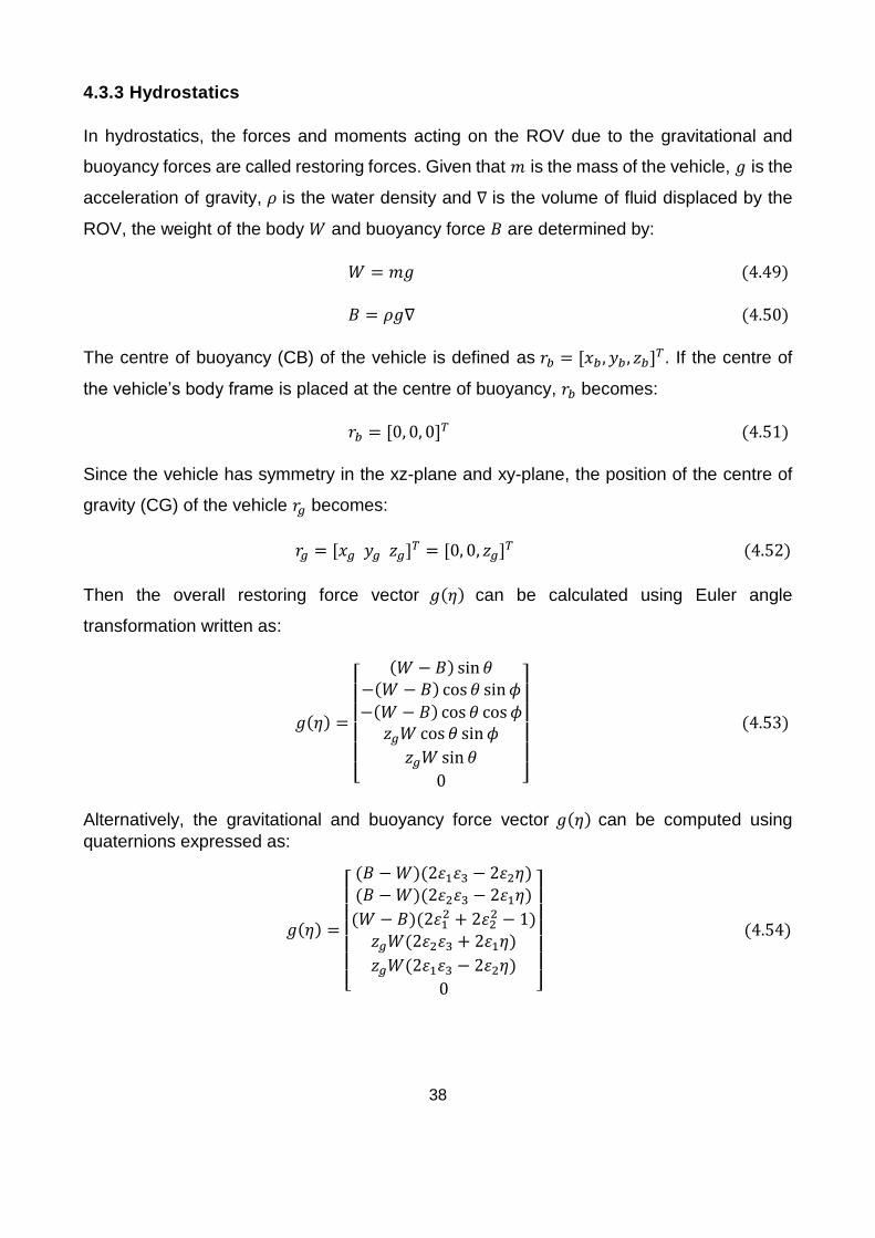
38
4.3.3 Hydrostatics
In hydrostatics, the forces and moments acting on the ROV due to the gravitational and
buoyancy forces are called restoring forces. Given that 𝑚 is the mass of the vehicle, 𝑔 is the
acceleration of gravity, 𝜌 is the water density and ∇ is the volume of fluid displaced by the
ROV, the weight of the body 𝑊 and buoyancy force 𝐵 are determined by:
𝑊 = 𝑚𝑔 (4.49)
𝐵 = 𝜌𝑔∇ (4.50)
The centre of buoyancy (CB) of the vehicle is defined as 𝑟𝑏 = [𝑥𝑏 , 𝑦𝑏 , 𝑧𝑏]𝑇. If the centre of
the vehicle’s body frame is placed at the centre of buoyancy, 𝑟𝑏 becomes:
𝑟𝑏 = [0, 0, 0]𝑇 (4.51)
Since the vehicle has symmetry in the xz-plane and xy-plane, the position of the centre of
gravity (CG) of the vehicle 𝑟𝑔 becomes:
𝑟𝑔 = [𝑥𝑔 𝑦𝑔 𝑧𝑔]𝑇 = [0, 0, 𝑧𝑔]
𝑇 (4.52)
Then the overall restoring force vector 𝑔(𝜂) can be calculated using Euler angle
transformation written as:
𝑔(𝜂) =
[
(𝑊 − 𝐵) sin 𝜃−(𝑊 − 𝐵) cos 𝜃 sin𝜙
−(𝑊 − 𝐵) cos 𝜃 cos𝜙𝑧𝑔𝑊cos 𝜃 sin𝜙
𝑧𝑔𝑊sin 𝜃
0 ]
(4.53)
Alternatively, the gravitational and buoyancy force vector 𝑔(𝜂) can be computed using
quaternions expressed as:
𝑔(𝜂) =
[ (𝐵 −𝑊)(2𝜀1𝜀3 − 2𝜀2𝜂)(𝐵 −𝑊)(2𝜀2𝜀3 − 2𝜀1𝜂)
(𝑊 − 𝐵)(2𝜀12 + 2𝜀2
2 − 1)𝑧𝑔𝑊(2𝜀2𝜀3 + 2𝜀1𝜂)
𝑧𝑔𝑊(2𝜀1𝜀3 − 2𝜀2𝜂)
0 ]
(4.54)
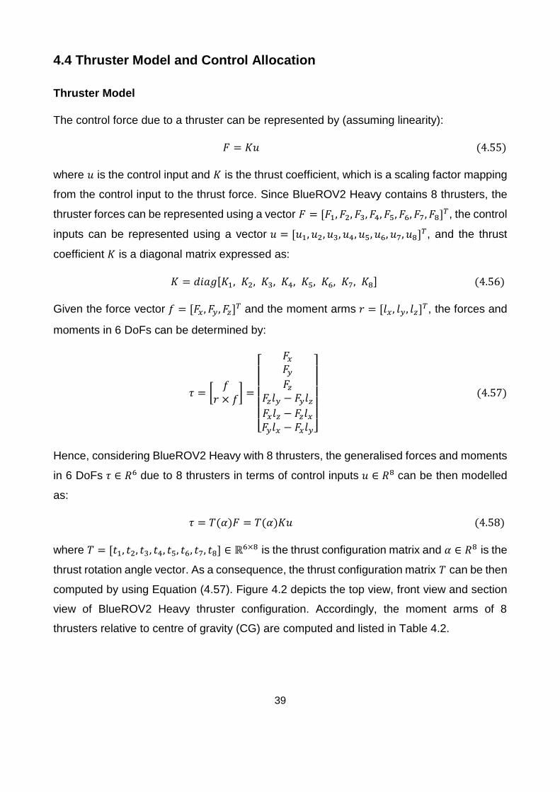
39
4.4 Thruster Model and Control Allocation
Thruster Model
The control force due to a thruster can be represented by (assuming linearity):
𝐹 = 𝐾𝑢 (4.55)
where 𝑢 is the control input and 𝐾 is the thrust coefficient, which is a scaling factor mapping
from the control input to the thrust force. Since BlueROV2 Heavy contains 8 thrusters, the
thruster forces can be represented using a vector 𝐹 = [𝐹1, 𝐹2, 𝐹3, 𝐹4, 𝐹5, 𝐹6, 𝐹7, 𝐹8]𝑇, the control
inputs can be represented using a vector 𝑢 = [𝑢1, 𝑢2, 𝑢3, 𝑢4, 𝑢5, 𝑢6, 𝑢7, 𝑢8]𝑇, and the thrust
coefficient 𝐾 is a diagonal matrix expressed as:
𝐾 = 𝑑𝑖𝑎𝑔[𝐾1, 𝐾2, 𝐾3, 𝐾4, 𝐾5, 𝐾6, 𝐾7, 𝐾8] (4.56)
Given the force vector 𝑓 = [𝐹𝑥 , 𝐹𝑦, 𝐹𝑧]𝑇 and the moment arms 𝑟 = [𝑙𝑥, 𝑙𝑦, 𝑙𝑧]
𝑇, the forces and
moments in 6 DoFs can be determined by:
𝜏 = [𝑓
𝑟 × 𝑓] =
[
𝐹𝑥𝐹𝑦𝐹𝑧
𝐹𝑧𝑙𝑦 − 𝐹𝑦𝑙𝑧𝐹𝑥𝑙𝑧 − 𝐹𝑧𝑙𝑥𝐹𝑦𝑙𝑥 − 𝐹𝑥𝑙𝑦]
(4.57)
Hence, considering BlueROV2 Heavy with 8 thrusters, the generalised forces and moments
in 6 DoFs 𝜏 ∈ 𝑅6 due to 8 thrusters in terms of control inputs 𝑢 ∈ 𝑅8 can be then modelled
as:
𝜏 = 𝑇(𝛼)𝐹 = 𝑇(𝛼)𝐾𝑢 (4.58)
where 𝑇 = [𝑡1, 𝑡2, 𝑡3, 𝑡4, 𝑡5, 𝑡6, 𝑡7, 𝑡8] ∈ ℝ6×8 is the thrust configuration matrix and 𝛼 ∈ 𝑅8 is the
thrust rotation angle vector. As a consequence, the thrust configuration matrix 𝑇 can be then
computed by using Equation (4.57). Figure 4.2 depicts the top view, front view and section
view of BlueROV2 Heavy thruster configuration. Accordingly, the moment arms of 8
thrusters relative to centre of gravity (CG) are computed and listed in Table 4.2.
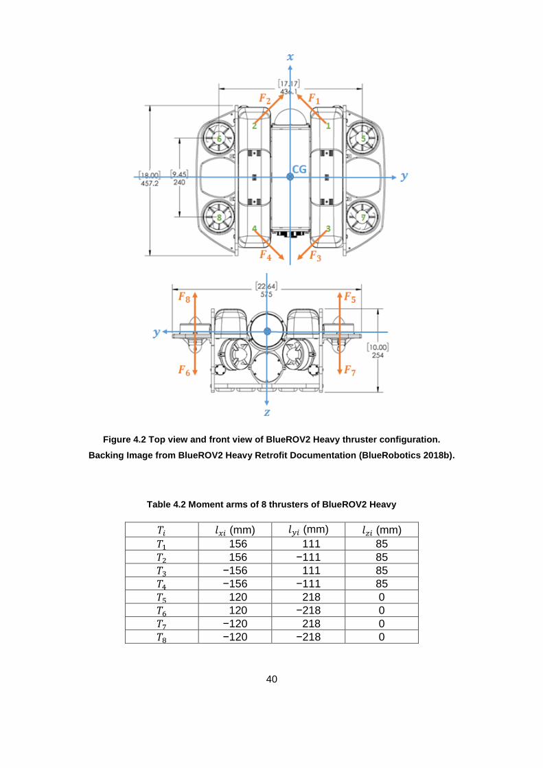
40
Figure 4.2 Top view and front view of BlueROV2 Heavy thruster configuration.
Backing Image from BlueROV2 Heavy Retrofit Documentation (BlueRobotics 2018b).
Table 4.2 Moment arms of 8 thrusters of BlueROV2 Heavy
𝑇𝑖 𝑙𝑥𝑖 (mm) 𝑙𝑦𝑖 (mm) 𝑙𝑧𝑖 (mm)
𝑇1 156 111 85
𝑇2 156 −111 85
𝑇3 −156 111 85
𝑇4 −156 −111 85
𝑇5 120 218 0
𝑇6 120 −218 0
𝑇7 −120 218 0
𝑇8 −120 −218 0
41
The rotation angles for horizontal thrusters of 𝑇1 to 𝑇4 are 𝜋/4 , −𝜋/4 , −3𝜋/4 and 3𝜋/4 ,
respectively and thruster 𝑇5 to 𝑇8 are vertical thrusters without horizontal rotations.
Subsequently, the forces and moments produced by thruster 𝑇1 can be computed by:
𝜏1 =
[
𝐹𝑥1𝐹𝑦1𝐹𝑧1
𝐹𝑧1𝑙𝑦1 − 𝐹𝑦1𝑙𝑧1𝐹𝑥1𝑙𝑧1 − 𝐹𝑧1𝑙𝑥1𝐹𝑦1𝑙𝑥1 − 𝐹𝑥1𝑙𝑦1]
=
[
𝐹1 cos(𝜋/4)−𝐹1 sin(𝜋/4)
0𝐹1 sin(𝜋/4) × 0.085𝐹1 cos(𝜋/4) × 0.085
−𝐹1 sin(𝜋/4) × 0.156 − 𝐹1 cos(𝜋/4) × 0.111]
=
[ 0.707−0.707
00.060.06
−0.1888]
𝐹1 (4.59)
Hence,
𝑡1 =
[ 0.707−0.707
00.060.06
−0.1888]
(4.60)
By following the same procedure, the forces and moments produced by total 8 thrusters are
found to be:
𝜏 = 𝑇(𝛼)𝐹 =
[ 0.707−0.707
00.060.06
−0.1888
0.7070.7070
−0.060.06
0.1888
−0.707−0.707
00.06−0.060.1888
−0.7070.7070
−0.06−0.06
−0.1888
00−1
−0.2180.1200
001
−0.218−0.120
0
001
0.2180.1200
00−1
0.218−0.120
0 ]
[ 𝐹1𝐹2𝐹3𝐹4𝐹5𝐹6𝐹7𝐹8]
(4.61)
Therefore, the thrust configuration matrix 𝑇 for BlueROV2 Heavy is given by:
𝑇 =
[ 0.707−0.707
00.060.06
−0.1888
0.7070.7070
−0.060.06
0.1888
−0.707−0.707
00.06−0.060.1888
−0.7070.7070
−0.06−0.06
−0.1888
00−1
−0.2180.1200
001
−0.218−0.120
0
001
0.2180.1200
00−1
0.218−0.120
0 ]
(4.62)
42
Control Allocation
Control allocation computes the control input signal 𝑢 to apply to the thrusters such that the
overall desired control forces 𝜏 can be generalised. Since the control forces and moments
due to thrusters with regard to control inputs are expressed by (4.58), the control input vector
can be derived as:
𝑢 = 𝐾−1𝑇−1𝜏 (4.63)
However, since the thrust configuration matrix 𝑇 for BlueROV2 Heavy is non-square, the
Moore-Penrose pseudo-inverse 𝑇+ is applied given by:
𝑇+ = 𝑇𝑇(𝑇𝑇𝑇)−1 (4.64)
Hence, the control input vector 𝑢 can be calculated as:
𝑢 = 𝐾−1𝑇+𝜏 (4.65)
4.5 Summary
The vectorial representation of dynamic model and the thruster model of BlueROV2 Heavy
has been presented in this chapter while assumptions were applied to simplify the complex
dynamic model. The derived models will be utilised extensively for the vehicle’s system
identification and control system design in the following chapters. The next chapter will
demonstrate the estimation of unknown parameters in the derived models.
43
CHAPTER 5
SYSTEM IDENTIFICATION
In order to identify the system property of the BlueROV2 Heavy, the parameters in the
dynamic and the thruster models derived in the last chapter need to be estimated. This
chapter firstly presents a system identification approach that could be performed in the
immersion tank with the use of on-board sensors. While the experimental platform is
currently not available for estimating parameters experimentally, necessary parameters are
determined by analysing the BlueROV2 Heavy’s technical specifications (BlueRobotics
2018b) and published literature relating to BlueROV (Sandøy 2016).
5.1 System Identification Approach
The experimental system identification of a complete ROV model requires a complete state
information that is complex, lengthy and expensive (Caccia, Indiveri et al. 2000). Several
schemes for estimating parameters in the ROV model have been reviewed in Section 2.4.
With the application of a system identification approach demonstrated in Indiveri (Indiveri
1998) and Caccia (Caccia, Indiveri et al. 2000), a methodology of immersion tank testing
system identification using on-board sensors is proposed to identify the parameters in the
dynamic model. This approach exploits the characteristics of the vehicle and assumes
decoupling between DoFs in hydrodynamics. As a consequence, each DoF can be
conducted independently and the experiments become highly repeatable. This approach
involves a combination of static and dynamic experiments for each DoF and then utilises
the least squares algorithm to estimate parameters from the experimental data.
Since each DoF can be treated individually, the dynamic model in Equation (4.2) can be
adapted to be written into a single DoF as the following:
𝑚𝜉�� + 𝑑𝜉𝜉 + 𝑑𝜉|𝜉|𝜉|𝜉| + 𝑔𝜉 = 𝜏𝜉 (5.1)
where 𝜉 is the velocity for a particular DoF, 𝑚𝜉 represents the system inertial parameter
containing rigid-body mass 𝑚𝑅𝐵,𝜉 and added mass 𝑚𝐴,𝜉 components, 𝑑𝜉 and 𝑑𝜉|𝜉| are the
44
linear and quadratic damping parameters, 𝑔𝜉 is the gravitational and buoyancy force and 𝜏𝜉
is the force applied to the vehicle; all the above parameters are for the considered DoF.
5.1.1 The Least Squares (LS) Technique
The least squares method is a commonly used regression analysis approach for
approximating unknown parameters from overdetermined systems of equations by
minimising the sum of residuals. Since the dynamic model in single DoF described in
Equation (5.1) is a linear expression with respect to the parameters, the LS technique is
used to estimate parameters for each DoF from a set of experimental data due to its ease
of implementation. Equation (5.1) can be expressed in a regression form given by:
𝑦 = 𝐻𝜃 (5.2)
where 𝑦 is a vector of known values, 𝐻 is a deterministic model matrix containing measured
data from experiments, and 𝜃 represents the parameter vector that needs to be estimated.
From the experimental data, the number of equations are larger than the number of unknown
parameters, which is an overdetermined system. The LS technique is used to estimate the
parameter 𝜃 by minimising the sum of squares of the residuals to fit the equations best. The
parameter can be then estimated by using the following equation (Indiveri 1998):
𝜃 = (𝐻𝑇𝐻)−1𝐻𝑇𝑦 (5.3)
Additionally, the standard deviation of the estimated parameter is calculated given by:
��𝜃 = √𝑑𝑖𝑎𝑔(𝐻𝑇𝐻)−1��2 (5.4)
where ��2 is the estimated Gaussian zero mean measurement noise variance given by:
��2 =(𝑦 − 𝐻𝜃)𝑇(𝑦 − 𝐻𝜃)
dim(𝑦) − dim (𝜃) (5.5)
The error of the estimated parameter is defined by:
𝜍 =��𝜃
|𝜃| (5.6)
45
5.1.2 Static Experiments
Static experiments are utilised to identify damping parameters that concern measuring the
velocity of the vehicle using on-board sensors when the steady-state speed condition holds.
In static experiments, a particular force for a specific DoF is applied to the vehicle, and when
the vehicle achieves the steady state speed, the velocity is constant whereas the
acceleration is zero. Under this condition, this constant velocity and this particular force are
recorded. For a single DoF, the dynamic model in (5.1) turns into:
𝑑𝜉𝜉 + 𝑑𝜉|𝜉|𝜉|𝜉| + 𝑔𝜉 = 𝜏𝜉 (5.7)
where �� = 0 and the system inertia term of 𝑚𝜉 is eliminated from the model. Since the force
𝜏𝜉 and the gravitational and buoyance 𝑔𝜉 are known, the linear damping term 𝑑𝜉 and the
quadratic damping term 𝑑𝜉|𝜉| are the only unknown parameters that can be estimated by
using the least squares technique for quadratic curve fitting of velocities 𝜉 and drag forces
(i.e. 𝜏𝜉 − 𝑔𝜉). In the expression of Equation (5.2), for 𝑛 inputs, the vector of known values 𝑦
are drag forces for the considered DoF turning into:
𝑦 = [
𝜏𝜉,1 − 𝑔𝜉𝜏𝜉,2 − 𝑔𝜉
⋮𝜏𝜉,𝑛 − 𝑔𝜉
] (5.8)
The matrix 𝐻 consists of the experimental data of constant velocities turning into:
𝐻 = [
𝜉1 𝜉1|𝜉1|𝜉2 𝜉2|𝜉2|
⋮𝜉𝑛 𝜉𝑛|𝜉𝑛|
] (5.9)
The unknown parameter vector 𝜃 of damping turns into:
𝜃 = [𝑑𝜉𝑑𝜉|𝜉|
] (5.10)
Hence, the damping parameters can be estimated using Equation (5.3). By applying the
same procedure for each 6 DoFs individually, damping parameters in 6 DoFs can be then
attained.
46
5.1.3 Dynamic Experiments
Dynamic experiments are employed to identify inertia parameters that involve measuring
the acceleration and velocity of the vehicle when the vehicle is accelerating. In dynamic
experiments, a sinusoidal force for a specific DoF is provided to the vehicle while measuring
the acceleration and the velocity of the vehicle using on-board sensors. Since the
parameters of damping terms have been identified in the static experiments, the remaining
parameters of the inertial term can now be determined. For a single DoF, the dynamic model
in (5.1) can be rearranged to the following:
𝑚𝜉�� = 𝜏𝜉 − 𝑔𝜉 − 𝑑𝜉𝜉 − 𝑑𝜉|𝜉|𝜉|𝜉| (5.11)
where terms of 𝜏𝜉, 𝑔𝜉, 𝑑𝜉 and 𝑑𝜉|𝜉| are known; therefore, the only unknown term of inertia
parameter 𝑚𝜉 can be estimated utilising the least squares technique where 𝑦,𝐻 and 𝜃 are
now turning into:
𝑦 =
[ 𝜏𝜉,1 − 𝑔𝜉 − 𝑑𝜉𝜉1 − 𝑑𝜉|𝜉|𝜉1|𝜉1|
𝜏𝜉,2 − 𝑔𝜉 − 𝑑𝜉𝜉2 − 𝑑𝜉|𝜉|𝜉2|𝜉2|
⋮𝜏𝜉,𝑛 − 𝑔𝜉 − 𝑑𝜉𝜉𝑛 − 𝑑𝜉|𝜉|𝜉𝑛|𝜉𝑛|]
(5.12)
𝐻 =
[ 𝜉1𝜉2⋮𝜉��]
(5.13)
𝜃 = 𝑚𝜉 (5.14)
Similarly, the system inertia parameter can be estimated using Equation (5.3). Note that the
system inertia parameter 𝑚𝜉 includes containing rigid-body mass 𝑚𝑅𝐵,𝜉 and added mass
𝑚𝐴,𝜉 where the rigid-body mass is known from an a priori information of measured data of
the vehicle. Hence, the added mass can be attained by:
𝑚𝐴,𝜉 = ��𝜉 −𝑚𝑅𝐵,𝜉 (5.15)
Likewise, by applying the same procedure for each 6 DoFs individually, system inertia
parameters in 6 DoFs can be obtained.
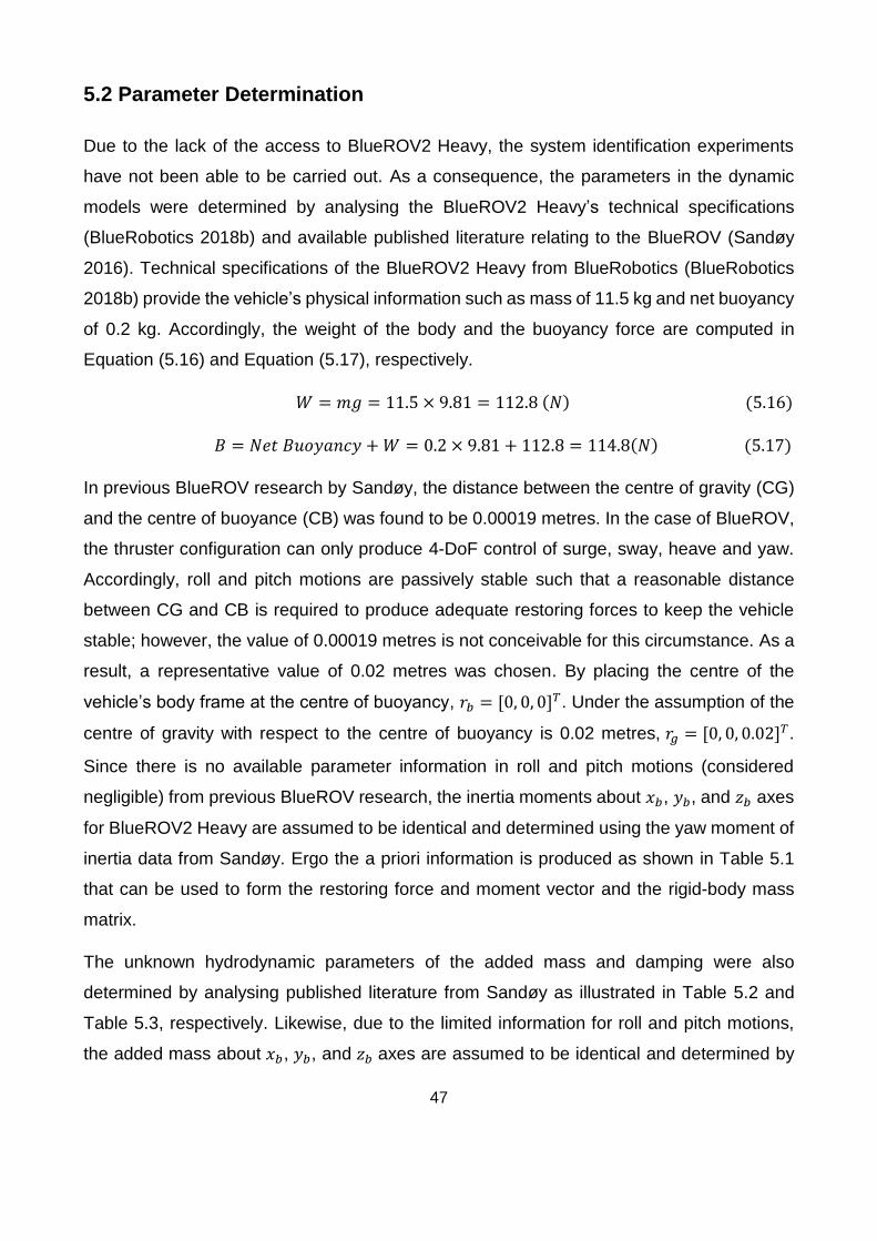
47
5.2 Parameter Determination
Due to the lack of the access to BlueROV2 Heavy, the system identification experiments
have not been able to be carried out. As a consequence, the parameters in the dynamic
models were determined by analysing the BlueROV2 Heavy’s technical specifications
(BlueRobotics 2018b) and available published literature relating to the BlueROV (Sandøy
2016). Technical specifications of the BlueROV2 Heavy from BlueRobotics (BlueRobotics
2018b) provide the vehicle’s physical information such as mass of 11.5 kg and net buoyancy
of 0.2 kg. Accordingly, the weight of the body and the buoyancy force are computed in
Equation (5.16) and Equation (5.17), respectively.
𝑊 = 𝑚𝑔 = 11.5 × 9.81 = 112.8 (𝑁) (5.16)
𝐵 = 𝑁𝑒𝑡 𝐵𝑢𝑜𝑦𝑎𝑛𝑐𝑦 +𝑊 = 0.2 × 9.81 + 112.8 = 114.8(𝑁) (5.17)
In previous BlueROV research by Sandøy, the distance between the centre of gravity (CG)
and the centre of buoyance (CB) was found to be 0.00019 metres. In the case of BlueROV,
the thruster configuration can only produce 4-DoF control of surge, sway, heave and yaw.
Accordingly, roll and pitch motions are passively stable such that a reasonable distance
between CG and CB is required to produce adequate restoring forces to keep the vehicle
stable; however, the value of 0.00019 metres is not conceivable for this circumstance. As a
result, a representative value of 0.02 metres was chosen. By placing the centre of the
vehicle’s body frame at the centre of buoyancy, 𝑟𝑏 = [0, 0, 0]𝑇. Under the assumption of the
centre of gravity with respect to the centre of buoyancy is 0.02 metres, 𝑟𝑔 = [0, 0, 0.02]𝑇.
Since there is no available parameter information in roll and pitch motions (considered
negligible) from previous BlueROV research, the inertia moments about 𝑥𝑏, 𝑦𝑏, and 𝑧𝑏 axes
for BlueROV2 Heavy are assumed to be identical and determined using the yaw moment of
inertia data from Sandøy. Ergo the a priori information is produced as shown in Table 5.1
that can be used to form the restoring force and moment vector and the rigid-body mass
matrix.
The unknown hydrodynamic parameters of the added mass and damping were also
determined by analysing published literature from Sandøy as illustrated in Table 5.2 and
Table 5.3, respectively. Likewise, due to the limited information for roll and pitch motions,
the added mass about 𝑥𝑏, 𝑦𝑏, and 𝑧𝑏 axes are assumed to be identical and determined by
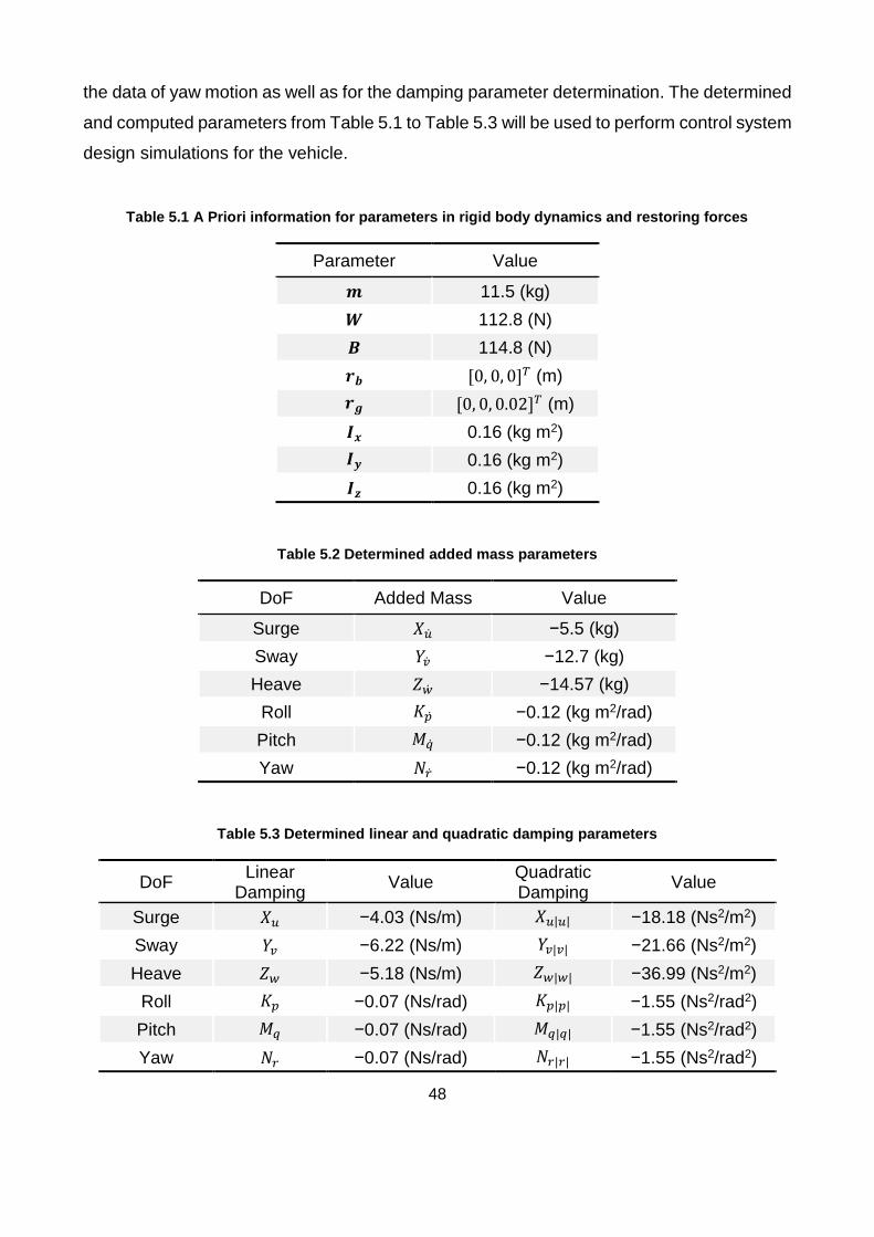
48
the data of yaw motion as well as for the damping parameter determination. The determined
and computed parameters from Table 5.1 to Table 5.3 will be used to perform control system
design simulations for the vehicle.
Table 5.1 A Priori information for parameters in rigid body dynamics and restoring forces
Parameter Value
𝒎 11.5 (kg)
𝑾 112.8 (N)
𝑩 114.8 (N)
𝒓𝒃 [0, 0, 0]𝑇 (m)
𝒓𝒈 [0, 0, 0.02]𝑇 (m)
𝑰𝒙 0.16 (kg m2)
𝑰𝒚 0.16 (kg m2)
𝑰𝒛 0.16 (kg m2)
Table 5.2 Determined added mass parameters
DoF Added Mass Value
Surge 𝑋�� −5.5 (kg)
Sway 𝑌�� −12.7 (kg)
Heave 𝑍�� −14.57 (kg)
Roll 𝐾�� −0.12 (kg m2/rad)
Pitch 𝑀�� −0.12 (kg m2/rad)
Yaw 𝑁�� −0.12 (kg m2/rad)
Table 5.3 Determined linear and quadratic damping parameters
DoF Linear
Damping Value
Quadratic Damping
Value
Surge 𝑋𝑢 −4.03 (Ns/m) 𝑋𝑢|𝑢| −18.18 (Ns2/m2)
Sway 𝑌𝑣 −6.22 (Ns/m) 𝑌𝑣|𝑣| −21.66 (Ns2/m2)
Heave 𝑍𝑤 −5.18 (Ns/m) 𝑍𝑤|𝑤| −36.99 (Ns2/m2)
Roll 𝐾𝑝 −0.07 (Ns/rad) 𝐾𝑝|𝑝| −1.55 (Ns2/rad2)
Pitch 𝑀𝑞 −0.07 (Ns/rad) 𝑀𝑞|𝑞| −1.55 (Ns2/rad2)
Yaw 𝑁𝑟 −0.07 (Ns/rad) 𝑁𝑟|𝑟| −1.55 (Ns2/rad2)
49
5.3 Thrust Identification
Since the thrust force applied to the ROV in the dynamic model is based on the control input
from the motors, it is necessary to identify the thrust coefficient that represents the mapping
from the control input signal to the thrust force. The thrust force can have considerable loss
due to the effect of thruster-thruster and thruster-hull interactions. Hence, the bollard pull
test in immersion tank is proposed to identify thrust characteristics experimentally. In this
test, BlueROV2 Heavy is attached to a bracket that is connected to a 6-axis load cell.
Thereupon, the thrust forces in 6-DoF are measured from the load cell while applying control
input signals to thruster motors. Thruster coefficients can then be estimated with the use of
the least squares technique explained in Section 5.1.
However, as BlueROV2 Heavy is not yet available for performing the immersion tank bollard
pull tests, the thrust coefficient is alternatively identified making use of thrust mappings data
of T200 thruster illustrated in Figure 5.1 provided by BlueRobotics (BlueRobotics 2018c) at
this stage. Within the PWM operating range, the map depicts linear relationships with input
signal and a zero thrust dead zone. The linear relationships are used to approximate the
thrust coefficient of Equation (4.56) in the thrust model of Equation (4.58) discussed in
Section 4.4. Since the eight thrusters of BlueROV2 Heavy are identical using T200 and the
maximum thrust produced is about 40 Newton at least (including forward and reverse
directions) at operating voltage of 16 V, the thrust coefficients of 𝐾1 to 𝐾8 in Equation (4.56)
are approximated to 40. Therefore, the thrust coefficient matrix 𝐾 is determined as below:
𝐾 = 𝑑𝑖𝑎𝑔[40, 40, 40, 40, 40, 40, 40, 40] (5.20)
5.4 Summary
In this chapter, a system identification approach of immersion tank testing has been
demonstrated for identifying parameters in the vehicle’s mathematical models derived in
Chapter 4. Although these tests could not be executed due to the unavailability of the
experimental platform, the unknown parameters were currently determined by making use
of the BlueROV2 Heavy’s technical specifications and published literature relating to the
BlueROV. The next chapter will then use these determined parameters to perform
simulations of control system design for BlueROV2 Heavy.
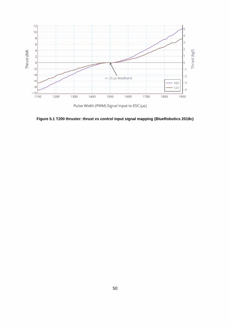
50
Figure 5.1 T200 thruster: thrust vs control input signal mapping (BlueRobotics 2018c)
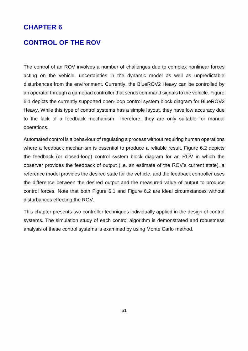
51
CHAPTER 6
CONTROL OF THE ROV
The control of an ROV involves a number of challenges due to complex nonlinear forces
acting on the vehicle, uncertainties in the dynamic model as well as unpredictable
disturbances from the environment. Currently, the BlueROV2 Heavy can be controlled by
an operator through a gamepad controller that sends command signals to the vehicle. Figure
6.1 depicts the currently supported open-loop control system block diagram for BlueROV2
Heavy. While this type of control systems has a simple layout, they have low accuracy due
to the lack of a feedback mechanism. Therefore, they are only suitable for manual
operations.
Automated control is a behaviour of regulating a process without requiring human operations
where a feedback mechanism is essential to produce a reliable result. Figure 6.2 depicts
the feedback (or closed-loop) control system block diagram for an ROV in which the
observer provides the feedback of output (i.e. an estimate of the ROV’s current state), a
reference model provides the desired state for the vehicle, and the feedback controller uses
the difference between the desired output and the measured value of output to produce
control forces. Note that both Figure 6.1 and Figure 6.2 are ideal circumstances without
disturbances effecting the ROV.
This chapter presents two controller techniques individually applied in the design of control
systems. The simulation study of each control algorithm is demonstrated and robustness
analysis of these control systems is examined by using Monte Carlo method.
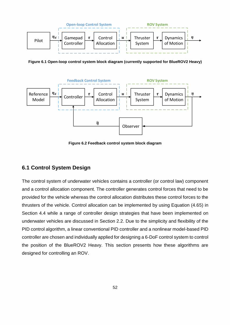
52
Gamepad Controller
Control Allocation
Thruster System
Dynamics of Motion
Pilot
Open-loop Control System ROV System
Figure 6.1 Open-loop control system block diagram (currently supported for BlueROV2 Heavy)
ControllerControl
AllocationThruster System
Dynamics of Motion
Observer
Reference Model
Feedback Control System ROV System
Figure 6.2 Feedback control system block diagram
6.1 Control System Design
The control system of underwater vehicles contains a controller (or control law) component
and a control allocation component. The controller generates control forces that need to be
provided for the vehicle whereas the control allocation distributes these control forces to the
thrusters of the vehicle. Control allocation can be implemented by using Equation (4.65) in
Section 4.4 while a range of controller design strategies that have been implemented on
underwater vehicles are discussed in Section 2.2. Due to the simplicity and flexibility of the
PID control algorithm, a linear conventional PID controller and a nonlinear model-based PID
controller are chosen and individually applied for designing a 6-DoF control system to control
the position of the BlueROV2 Heavy. This section presents how these algorithms are
designed for controlling an ROV.
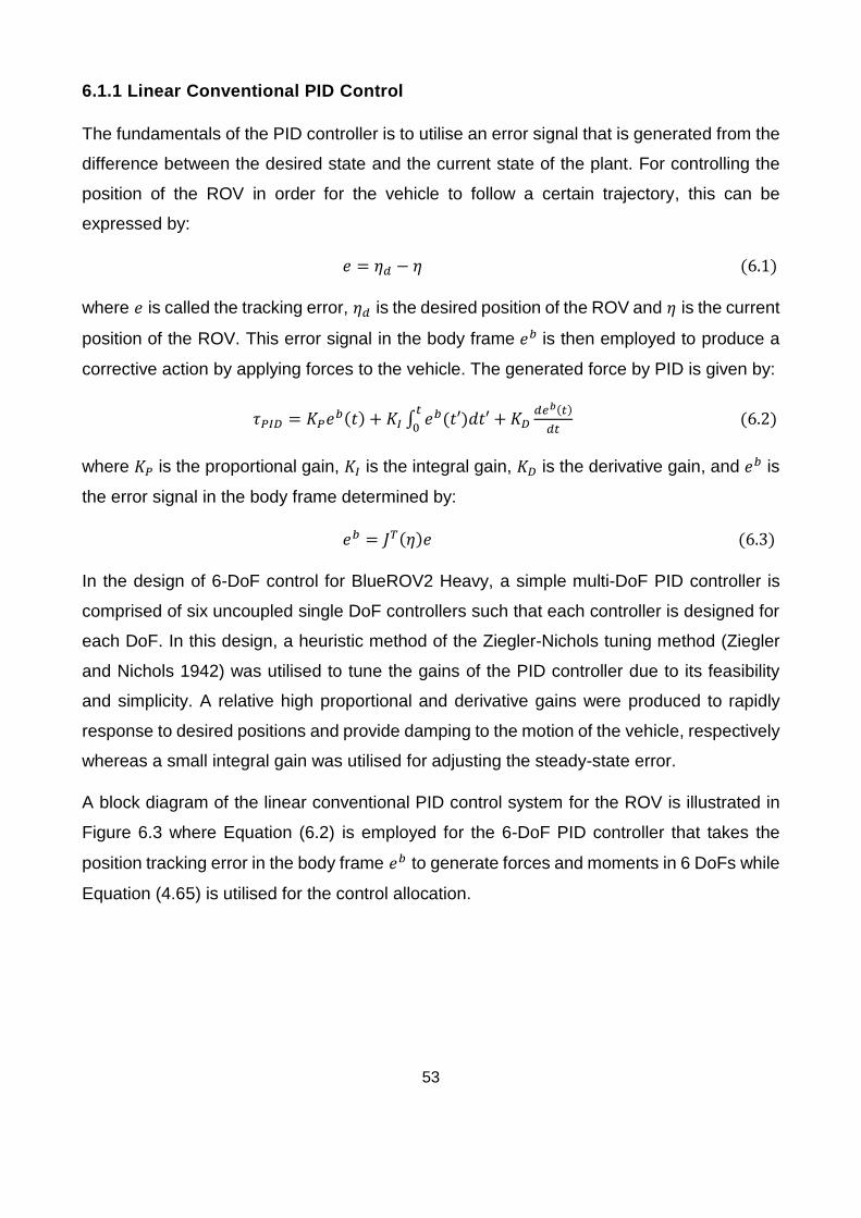
53
6.1.1 Linear Conventional PID Control
The fundamentals of the PID controller is to utilise an error signal that is generated from the
difference between the desired state and the current state of the plant. For controlling the
position of the ROV in order for the vehicle to follow a certain trajectory, this can be
expressed by:
𝑒 = 𝜂𝑑 − 𝜂 (6.1)
where 𝑒 is called the tracking error, 𝜂𝑑 is the desired position of the ROV and 𝜂 is the current
position of the ROV. This error signal in the body frame 𝑒𝑏 is then employed to produce a
corrective action by applying forces to the vehicle. The generated force by PID is given by:
𝜏𝑃𝐼𝐷 = 𝐾𝑃𝑒𝑏(𝑡) + 𝐾𝐼 ∫ 𝑒𝑏(𝑡′)𝑑𝑡′
𝑡
0+𝐾𝐷
𝑑𝑒𝑏(𝑡)
𝑑𝑡 (6.2)
where 𝐾𝑃 is the proportional gain, 𝐾𝐼 is the integral gain, 𝐾𝐷 is the derivative gain, and 𝑒𝑏 is
the error signal in the body frame determined by:
𝑒𝑏 = 𝐽𝑇(𝜂)𝑒 (6.3)
In the design of 6-DoF control for BlueROV2 Heavy, a simple multi-DoF PID controller is
comprised of six uncoupled single DoF controllers such that each controller is designed for
each DoF. In this design, a heuristic method of the Ziegler-Nichols tuning method (Ziegler
and Nichols 1942) was utilised to tune the gains of the PID controller due to its feasibility
and simplicity. A relative high proportional and derivative gains were produced to rapidly
response to desired positions and provide damping to the motion of the vehicle, respectively
whereas a small integral gain was utilised for adjusting the steady-state error.
A block diagram of the linear conventional PID control system for the ROV is illustrated in
Figure 6.3 where Equation (6.2) is employed for the 6-DoF PID controller that takes the
position tracking error in the body frame 𝑒𝑏 to generate forces and moments in 6 DoFs while
Equation (4.65) is utilised for the control allocation.
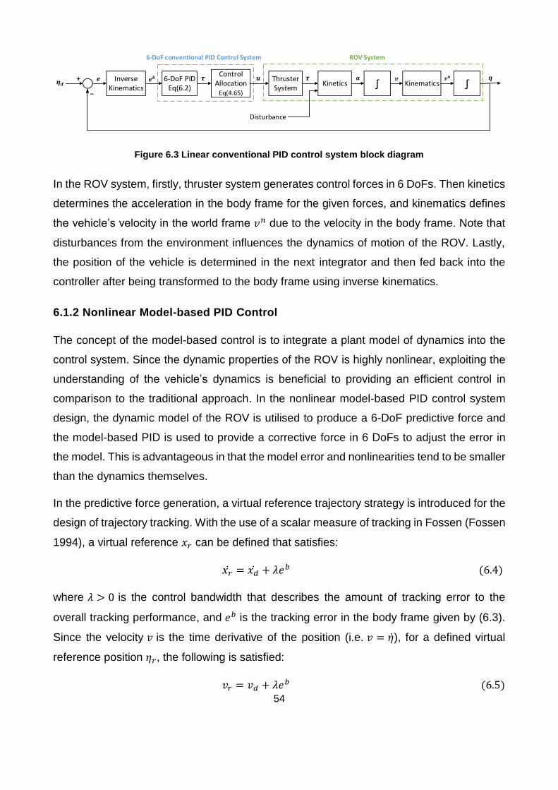
54
6-DoF conventional PID Control System ROV System
𝒃 6-DoF PID Eq(6.2)
Control Allocation
Eq(4.65)
Inverse Kinematics
Thruster System
Kinetics Kinematics
Disturbance
Figure 6.3 Linear conventional PID control system block diagram
In the ROV system, firstly, thruster system generates control forces in 6 DoFs. Then kinetics
determines the acceleration in the body frame for the given forces, and kinematics defines
the vehicle’s velocity in the world frame 𝑣𝑛 due to the velocity in the body frame. Note that
disturbances from the environment influences the dynamics of motion of the ROV. Lastly,
the position of the vehicle is determined in the next integrator and then fed back into the
controller after being transformed to the body frame using inverse kinematics.
6.1.2 Nonlinear Model-based PID Control
The concept of the model-based control is to integrate a plant model of dynamics into the
control system. Since the dynamic properties of the ROV is highly nonlinear, exploiting the
understanding of the vehicle’s dynamics is beneficial to providing an efficient control in
comparison to the traditional approach. In the nonlinear model-based PID control system
design, the dynamic model of the ROV is utilised to produce a 6-DoF predictive force and
the model-based PID is used to provide a corrective force in 6 DoFs to adjust the error in
the model. This is advantageous in that the model error and nonlinearities tend to be smaller
than the dynamics themselves.
In the predictive force generation, a virtual reference trajectory strategy is introduced for the
design of trajectory tracking. With the use of a scalar measure of tracking in Fossen (Fossen
1994), a virtual reference 𝑥𝑟 can be defined that satisfies:
𝑥�� = 𝑥�� + 𝜆𝑒𝑏 (6.4)
where 𝜆 > 0 is the control bandwidth that describes the amount of tracking error to the
overall tracking performance, and 𝑒𝑏 is the tracking error in the body frame given by (6.3).
Since the velocity 𝑣 is the time derivative of the position (i.e. 𝑣 = ��), for a defined virtual
reference position 𝜂𝑟, the following is satisfied:
𝑣𝑟 = 𝑣𝑑 + 𝜆𝑒𝑏 (6.5)
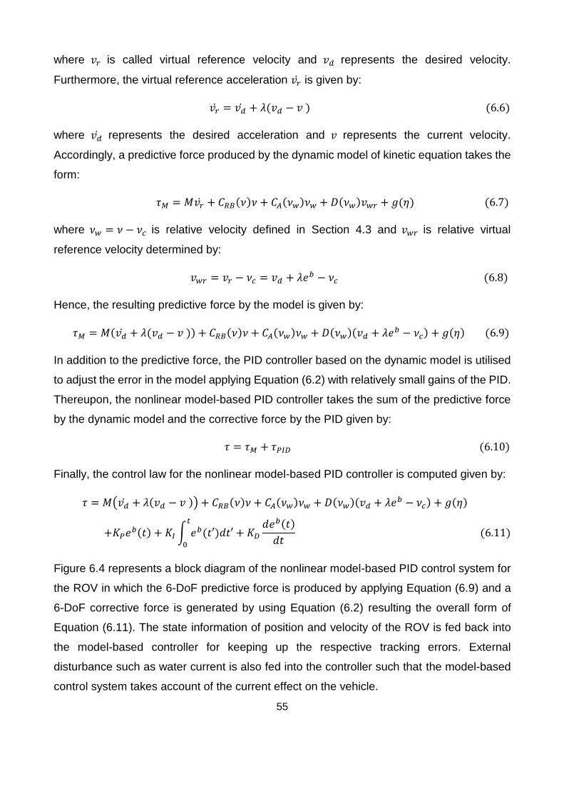
55
where 𝑣𝑟 is called virtual reference velocity and 𝑣𝑑 represents the desired velocity.
Furthermore, the virtual reference acceleration 𝑣�� is given by:
𝑣�� = 𝑣�� + 𝜆(𝑣𝑑 − 𝑣 ) (6.6)
where 𝑣�� represents the desired acceleration and 𝑣 represents the current velocity.
Accordingly, a predictive force produced by the dynamic model of kinetic equation takes the
form:
𝜏𝑀 = 𝑀𝑣�� + 𝐶𝑅𝐵(𝜈)𝜈 + 𝐶𝐴(𝜈𝑤)𝜈𝑤 + 𝐷(𝜈𝑤)𝑣𝑤𝑟 + 𝑔(𝜂) (6.7)
where 𝜈𝑤 = 𝜈 − 𝜈𝑐 is relative velocity defined in Section 4.3 and 𝑣𝑤𝑟 is relative virtual
reference velocity determined by:
𝑣𝑤𝑟 = 𝑣𝑟 − 𝜈𝑐 = 𝑣𝑑 + 𝜆𝑒𝑏 − 𝜈𝑐 (6.8)
Hence, the resulting predictive force by the model is given by:
𝜏𝑀 = 𝑀(𝑣�� + 𝜆(𝑣𝑑 − 𝑣 )) + 𝐶𝑅𝐵(𝜈)𝜈 + 𝐶𝐴(𝜈𝑤)𝜈𝑤 + 𝐷(𝜈𝑤)(𝑣𝑑 + 𝜆𝑒𝑏 − 𝜈𝑐) + 𝑔(𝜂) (6.9)
In addition to the predictive force, the PID controller based on the dynamic model is utilised
to adjust the error in the model applying Equation (6.2) with relatively small gains of the PID.
Thereupon, the nonlinear model-based PID controller takes the sum of the predictive force
by the dynamic model and the corrective force by the PID given by:
𝜏 = 𝜏𝑀 + 𝜏𝑃𝐼𝐷 (6.10)
Finally, the control law for the nonlinear model-based PID controller is computed given by:
𝜏 = 𝑀(𝑣�� + 𝜆(𝑣𝑑 − 𝑣 )) + 𝐶𝑅𝐵(𝜈)𝜈 + 𝐶𝐴(𝜈𝑤)𝜈𝑤 + 𝐷(𝜈𝑤)(𝑣𝑑 + 𝜆𝑒𝑏 − 𝜈𝑐) + 𝑔(𝜂)
+𝐾𝑃𝑒𝑏(𝑡) + 𝐾𝐼 ∫ 𝑒𝑏(𝑡′)𝑑𝑡′
𝑡
0
+ 𝐾𝐷
𝑑𝑒𝑏(𝑡)
𝑑𝑡 (6.11)
Figure 6.4 represents a block diagram of the nonlinear model-based PID control system for
the ROV in which the 6-DoF predictive force is produced by applying Equation (6.9) and a
6-DoF corrective force is generated by using Equation (6.2) resulting the overall form of
Equation (6.11). The state information of position and velocity of the ROV is fed back into
the model-based controller for keeping up the respective tracking errors. External
disturbance such as water current is also fed into the controller such that the model-based
control system takes account of the current effect on the vehicle.
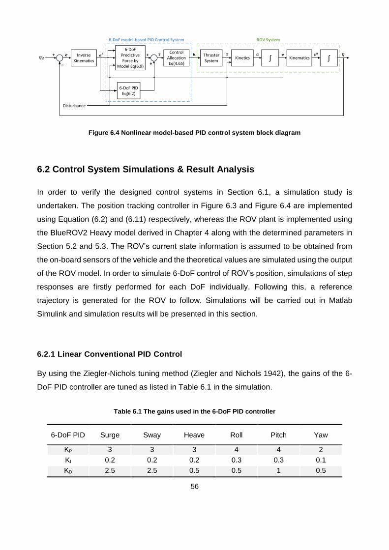
56
6-DoF model-based PID Control System ROV System
𝒃Control
Allocation Eq(4.65)
Inverse Kinematics
Thruster System
Kinetics Kinematics
Disturbance
6-DoF PID Eq(6.2)
6-DoF Predictive Force by
Model Eq(6.9)
Figure 6.4 Nonlinear model-based PID control system block diagram
6.2 Control System Simulations & Result Analysis
In order to verify the designed control systems in Section 6.1, a simulation study is
undertaken. The position tracking controller in Figure 6.3 and Figure 6.4 are implemented
using Equation (6.2) and (6.11) respectively, whereas the ROV plant is implemented using
the BlueROV2 Heavy model derived in Chapter 4 along with the determined parameters in
Section 5.2 and 5.3. The ROV’s current state information is assumed to be obtained from
the on-board sensors of the vehicle and the theoretical values are simulated using the output
of the ROV model. In order to simulate 6-DoF control of ROV’s position, simulations of step
responses are firstly performed for each DoF individually. Following this, a reference
trajectory is generated for the ROV to follow. Simulations will be carried out in Matlab
Simulink and simulation results will be presented in this section.
6.2.1 Linear Conventional PID Control
By using the Ziegler-Nichols tuning method (Ziegler and Nichols 1942), the gains of the 6-
DoF PID controller are tuned as listed in Table 6.1 in the simulation.
Table 6.1 The gains used in the 6-DoF PID controller
6-DoF PID Surge Sway Heave Roll Pitch Yaw
KP 3 3 3 4 4 2
KI 0.2 0.2 0.2 0.3 0.3 0.1
KD 2.5 2.5 0.5 0.5 1 0.5
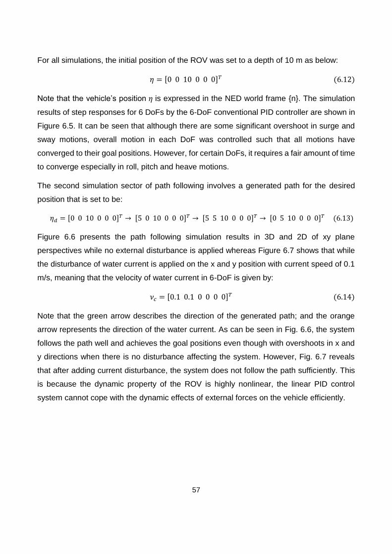
57
For all simulations, the initial position of the ROV was set to a depth of 10 m as below:
𝜂 = [0 0 10 0 0 0]𝑇 (6.12)
Note that the vehicle’s position 𝜂 is expressed in the NED world frame {n}. The simulation
results of step responses for 6 DoFs by the 6-DoF conventional PID controller are shown in
Figure 6.5. It can be seen that although there are some significant overshoot in surge and
sway motions, overall motion in each DoF was controlled such that all motions have
converged to their goal positions. However, for certain DoFs, it requires a fair amount of time
to converge especially in roll, pitch and heave motions.
The second simulation sector of path following involves a generated path for the desired
position that is set to be:
𝜂𝑑 = [0 0 10 0 0 0]𝑇 → [5 0 10 0 0 0]𝑇 → [5 5 10 0 0 0]𝑇 → [0 5 10 0 0 0]𝑇 (6.13)
Figure 6.6 presents the path following simulation results in 3D and 2D of xy plane
perspectives while no external disturbance is applied whereas Figure 6.7 shows that while
the disturbance of water current is applied on the x and y position with current speed of 0.1
m/s, meaning that the velocity of water current in 6-DoF is given by:
𝜈𝑐 = [0.1 0.1 0 0 0 0]𝑇 (6.14)
Note that the green arrow describes the direction of the generated path; and the orange
arrow represents the direction of the water current. As can be seen in Fig. 6.6, the system
follows the path well and achieves the goal positions even though with overshoots in x and
y directions when there is no disturbance affecting the system. However, Fig. 6.7 reveals
that after adding current disturbance, the system does not follow the path sufficiently. This
is because the dynamic property of the ROV is highly nonlinear, the linear PID control
system cannot cope with the dynamic effects of external forces on the vehicle efficiently.
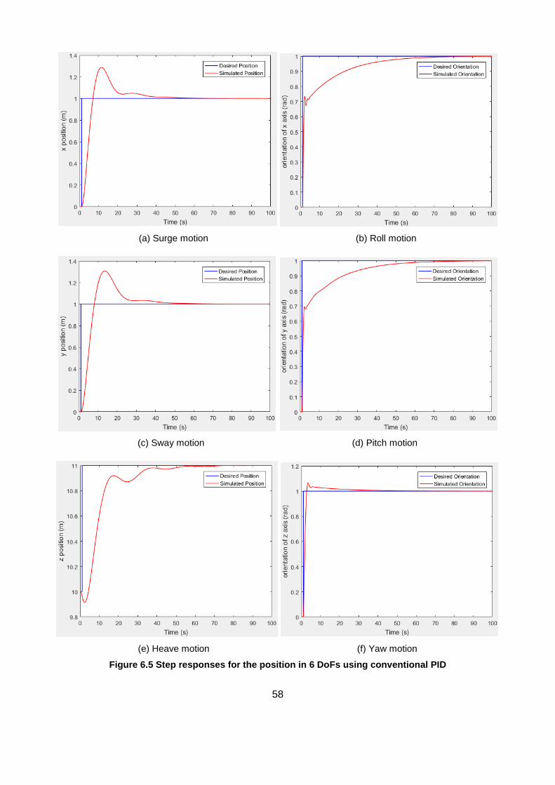
58
(a) Surge motion (b) Roll motion
(c) Sway motion (d) Pitch motion
(e) Heave motion (f) Yaw motion
Figure 6.5 Step responses for the position in 6 DoFs using conventional PID
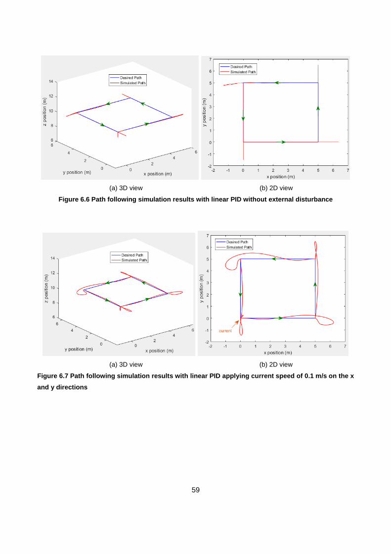
59
(a) 3D view (b) 2D view
Figure 6.6 Path following simulation results with linear PID without external disturbance
(a) 3D view (b) 2D view
Figure 6.7 Path following simulation results with linear PID applying current speed of 0.1 m/s on the x
and y directions
60
6.2.2 Nonlinear Model-based PID Control
Likewise, with the use of the Ziegler-Nichols tuning method (Ziegler and Nichols 1942), the
gains of the 6-DoF model-based PID controller are tuned as listed in Table 6.2. It can be
seen that the used gains of the model-based PID are relatively small compared with the
gains in Table 6.1. This is because in the model-based control system, the majority of control
forces is contributed from the predictive force by the ROV’s dynamic model and the residual
error is corrected by the PID controller.
Similarly, step response simulations for 6 DoFs were performed firstly as the results shown
in Figure 6.8. It is noticeable that the model-based PID control system produces slight
overshoot and achieves the goal positions quickly. These features are highly desirable since
the vehicle does not require significant direction reverse to accomplish the desired position
and demands relatively small energy which results in efficient performance.
Next, the path following simulation results by the nonlinear model-based PID control system
without external disturbance applied are shown in Figure 6.9 whereas Figure 6.10 presents
the path following simulation results when a water current disturbance is applied on the x
and y position with current speed of 0.1 m/s described by Equation (6.14). It can be seen
that simulations results in Fig. 6.9 and Fig. 6.10 are almost identical, with sufficient
performance, meaning that the system has high level of resistance to current disturbance at
speed of 0.1 m/s. This is because the model-based control system exploits the dynamic
model of the ROV so that considers the nonlinearity of the dynamic effects by the
disturbance.
Table 6.2 The gains used in the 6-DoF model-based PID controller
6-DoF PID Surge Sway Heave Roll Pitch Yaw
KP 1 1 1.2 0.3 0.3 0.3
KI 0.001 0.001 0.001 0.001 0.001 0.001
KD 0 0 0 0.3 0.3 0.3
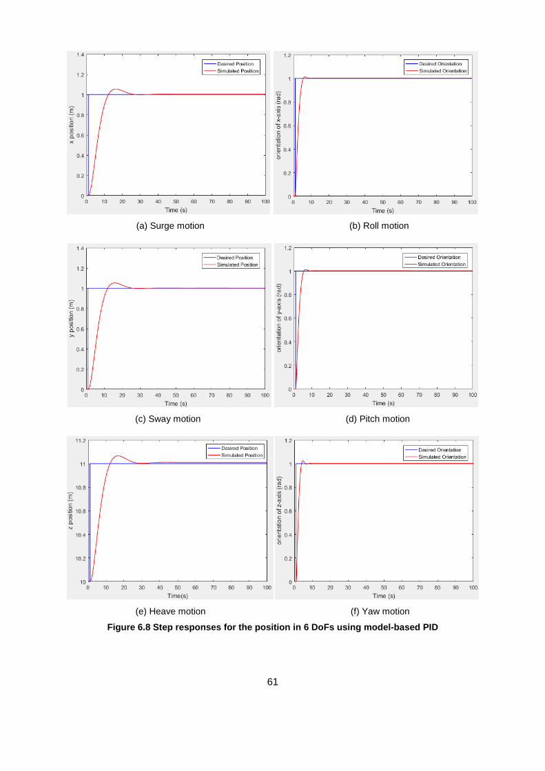
61
(a) Surge motion (b) Roll motion
(c) Sway motion (d) Pitch motion
(e) Heave motion (f) Yaw motion
Figure 6.8 Step responses for the position in 6 DoFs using model-based PID
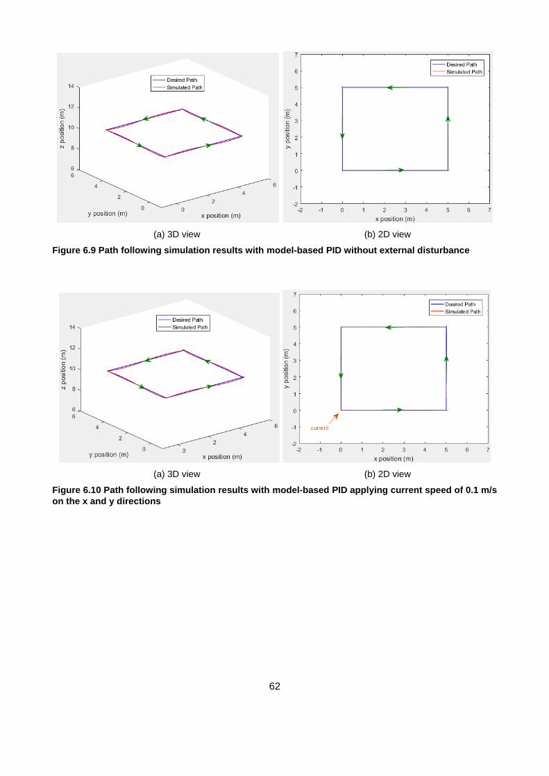
62
(a) 3D view (b) 2D view
Figure 6.9 Path following simulation results with model-based PID without external disturbance
(a) 3D view (b) 2D view
Figure 6.10 Path following simulation results with model-based PID applying current speed of 0.1 m/s
on the x and y directions
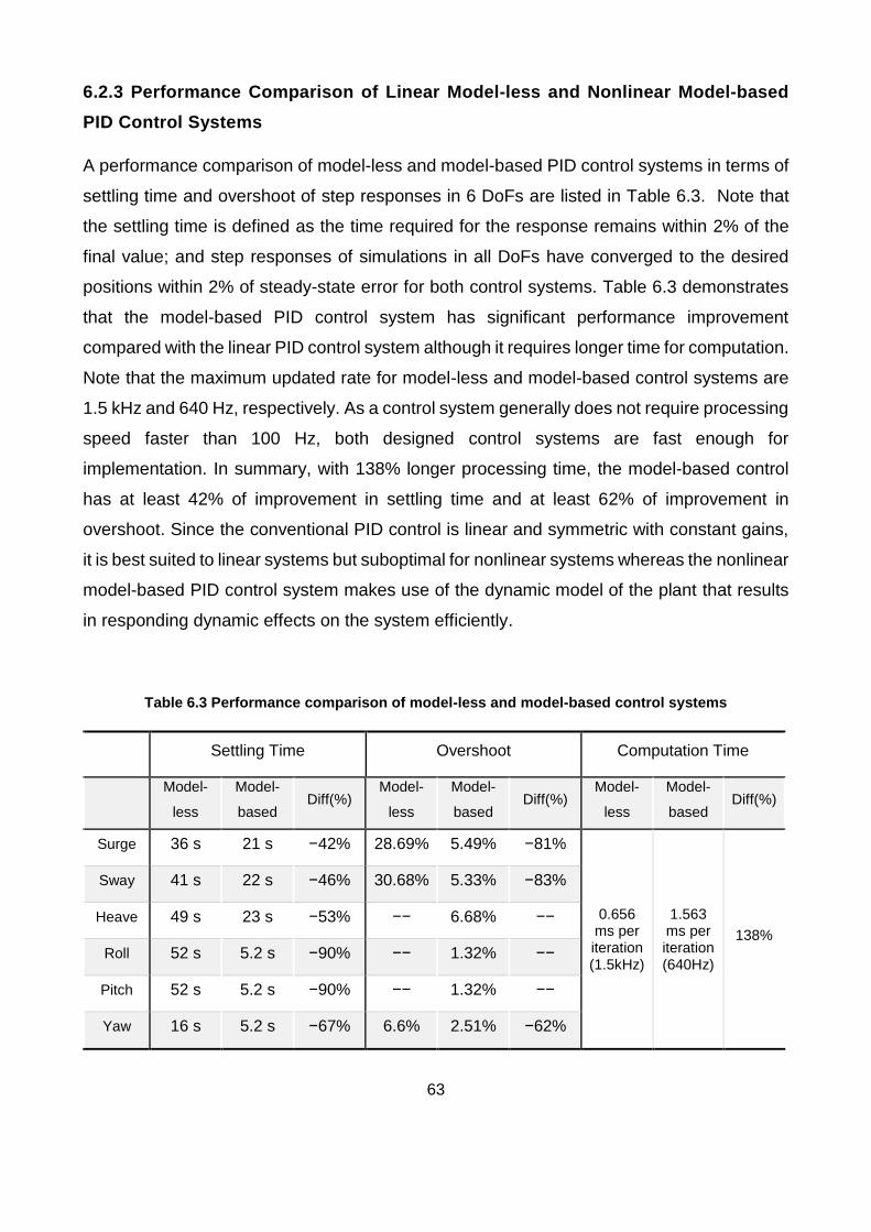
63
6.2.3 Performance Comparison of Linear Model-less and Nonlinear Model-based
PID Control Systems
A performance comparison of model-less and model-based PID control systems in terms of
settling time and overshoot of step responses in 6 DoFs are listed in Table 6.3. Note that
the settling time is defined as the time required for the response remains within 2% of the
final value; and step responses of simulations in all DoFs have converged to the desired
positions within 2% of steady-state error for both control systems. Table 6.3 demonstrates
that the model-based PID control system has significant performance improvement
compared with the linear PID control system although it requires longer time for computation.
Note that the maximum updated rate for model-less and model-based control systems are
1.5 kHz and 640 Hz, respectively. As a control system generally does not require processing
speed faster than 100 Hz, both designed control systems are fast enough for
implementation. In summary, with 138% longer processing time, the model-based control
has at least 42% of improvement in settling time and at least 62% of improvement in
overshoot. Since the conventional PID control is linear and symmetric with constant gains,
it is best suited to linear systems but suboptimal for nonlinear systems whereas the nonlinear
model-based PID control system makes use of the dynamic model of the plant that results
in responding dynamic effects on the system efficiently.
Table 6.3 Performance comparison of model-less and model-based control systems
Settling Time Overshoot Computation Time
Model-
less
Model-
based Diff(%)
Model-
less
Model-
based Diff(%)
Model-
less
Model-
based Diff(%)
Surge 36 s 21 s −42% 28.69% 5.49% −81%
0.656 ms per iteration (1.5kHz)
1.563 ms per iteration (640Hz)
138%
Sway 41 s 22 s −46% 30.68% 5.33% −83%
Heave 49 s 23 s −53% −− 6.68% −−
Roll 52 s 5.2 s −90% −− 1.32% −−
Pitch 52 s 5.2 s −90% −− 1.32% −−
Yaw 16 s 5.2 s −67% 6.6% 2.51% −62%
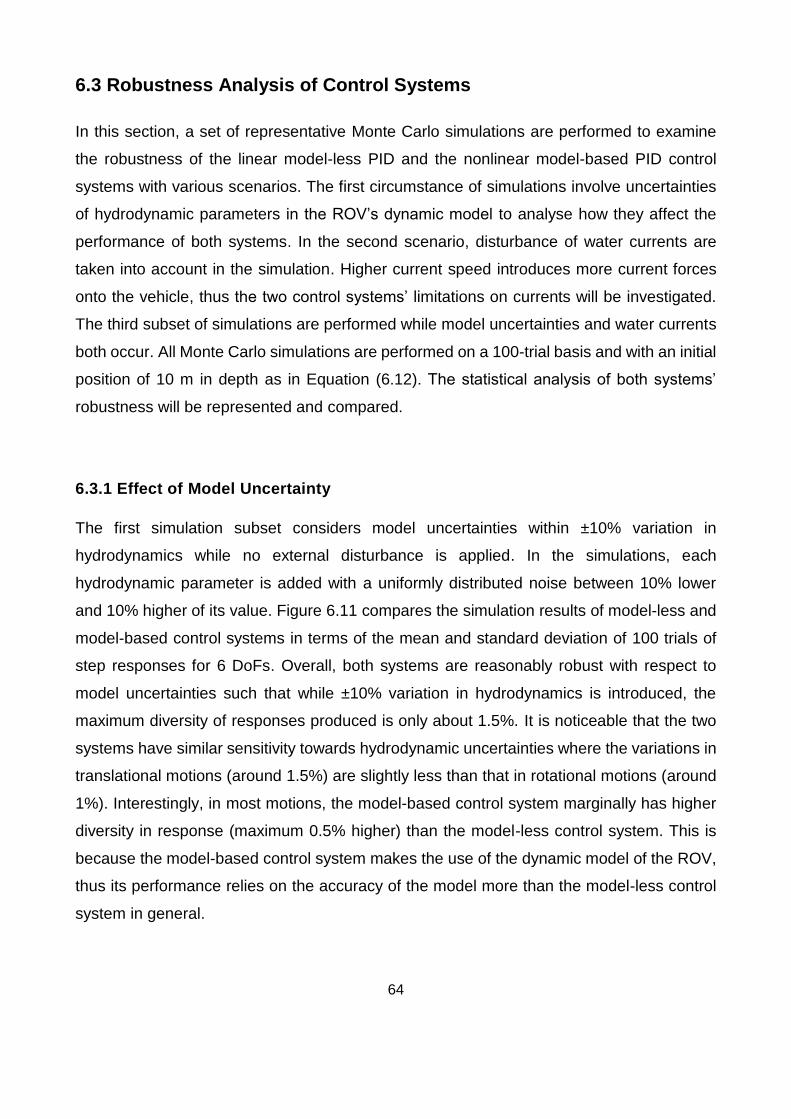
64
6.3 Robustness Analysis of Control Systems
In this section, a set of representative Monte Carlo simulations are performed to examine
the robustness of the linear model-less PID and the nonlinear model-based PID control
systems with various scenarios. The first circumstance of simulations involve uncertainties
of hydrodynamic parameters in the ROV’s dynamic model to analyse how they affect the
performance of both systems. In the second scenario, disturbance of water currents are
taken into account in the simulation. Higher current speed introduces more current forces
onto the vehicle, thus the two control systems’ limitations on currents will be investigated.
The third subset of simulations are performed while model uncertainties and water currents
both occur. All Monte Carlo simulations are performed on a 100-trial basis and with an initial
position of 10 m in depth as in Equation (6.12). The statistical analysis of both systems’
robustness will be represented and compared.
6.3.1 Effect of Model Uncertainty
The first simulation subset considers model uncertainties within ±10% variation in
hydrodynamics while no external disturbance is applied. In the simulations, each
hydrodynamic parameter is added with a uniformly distributed noise between 10% lower
and 10% higher of its value. Figure 6.11 compares the simulation results of model-less and
model-based control systems in terms of the mean and standard deviation of 100 trials of
step responses for 6 DoFs. Overall, both systems are reasonably robust with respect to
model uncertainties such that while ±10% variation in hydrodynamics is introduced, the
maximum diversity of responses produced is only about 1.5%. It is noticeable that the two
systems have similar sensitivity towards hydrodynamic uncertainties where the variations in
translational motions (around 1.5%) are slightly less than that in rotational motions (around
1%). Interestingly, in most motions, the model-based control system marginally has higher
diversity in response (maximum 0.5% higher) than the model-less control system. This is
because the model-based control system makes the use of the dynamic model of the ROV,
thus its performance relies on the accuracy of the model more than the model-less control
system in general.
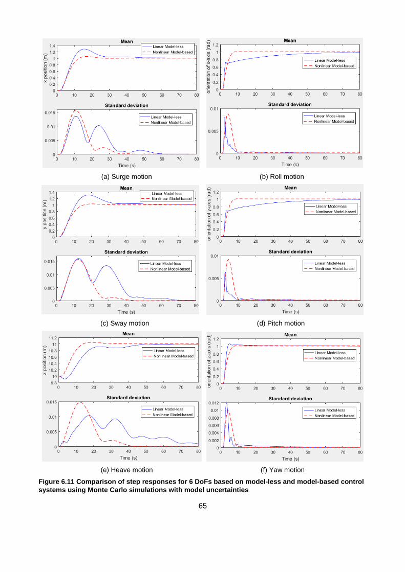
65
(a) Surge motion (b) Roll motion
(c) Sway motion (d) Pitch motion
(e) Heave motion (f) Yaw motion
Figure 6.11 Comparison of step responses for 6 DoFs based on model-less and model-based control
systems using Monte Carlo simulations with model uncertainties
66
6.3.2 Effect of Current Disturbance
This second study investigates the effect of environmental disturbance of currents on the
performance of the designed control systems while the model uncertainty is not considered.
Since the ocean current is commonly assumed to be constant and irrotational in the inertial
frame when describing its effects on marine vehicles (Fossen 2011), a water current is
generated in the x, y and z directions in the simulations. The current velocity is set to 0.25
m/s with an added uniformly distributed noise 𝜀 between 10% lower and 10% higher of the
current speed. Hence, the velocity of water current in 6-DoF is given by:
𝜈𝑐 = [0.25 + 𝜀, 0.25 + 𝜀, 0.25 + 𝜀, 0, 0, 0]𝑇 (6.15)
Figure 6.12 compares the simulation results of using model-less and model-based control
systems in presenting the mean and standard deviation of 100 trials of step responses in 6
DoFs. It can be seen that the water current affects the performance of the model-less control
system considerably in terms of settling time and overshoot where it takes much longer (over
1.5 times) to converge in most DoFs (surge, sway, heave and yaw) after applying current,
and the overshoot in translational motions have increased dramatically (to between 55%
and 97%). On the other hand, the model-based control system shows its sufficient
robustness in regard to current disturbance such that its performance remains with similar
settling time in all DoFs and reduced overshoot in some DoFs (surge, sway and yaw) in the
presence of water current. In addition, with ±10% variation of the current speed, the
maximum diversity of responses produced by the model-based control system is only about
1% whereas that is about 7.5% by the model-less system.
Since the model-based control system exploits the dynamic model and considers the
nonlinearity of the current effect on the vehicle, the error for linearisation in the model-based
PID controller is much smaller than that in the model-less PID controller. Hence, the model-
based control system results in a much more accurate control behaviour and performance
whereas the model-less control system is only effective for a relatively small range from the
tuning point.
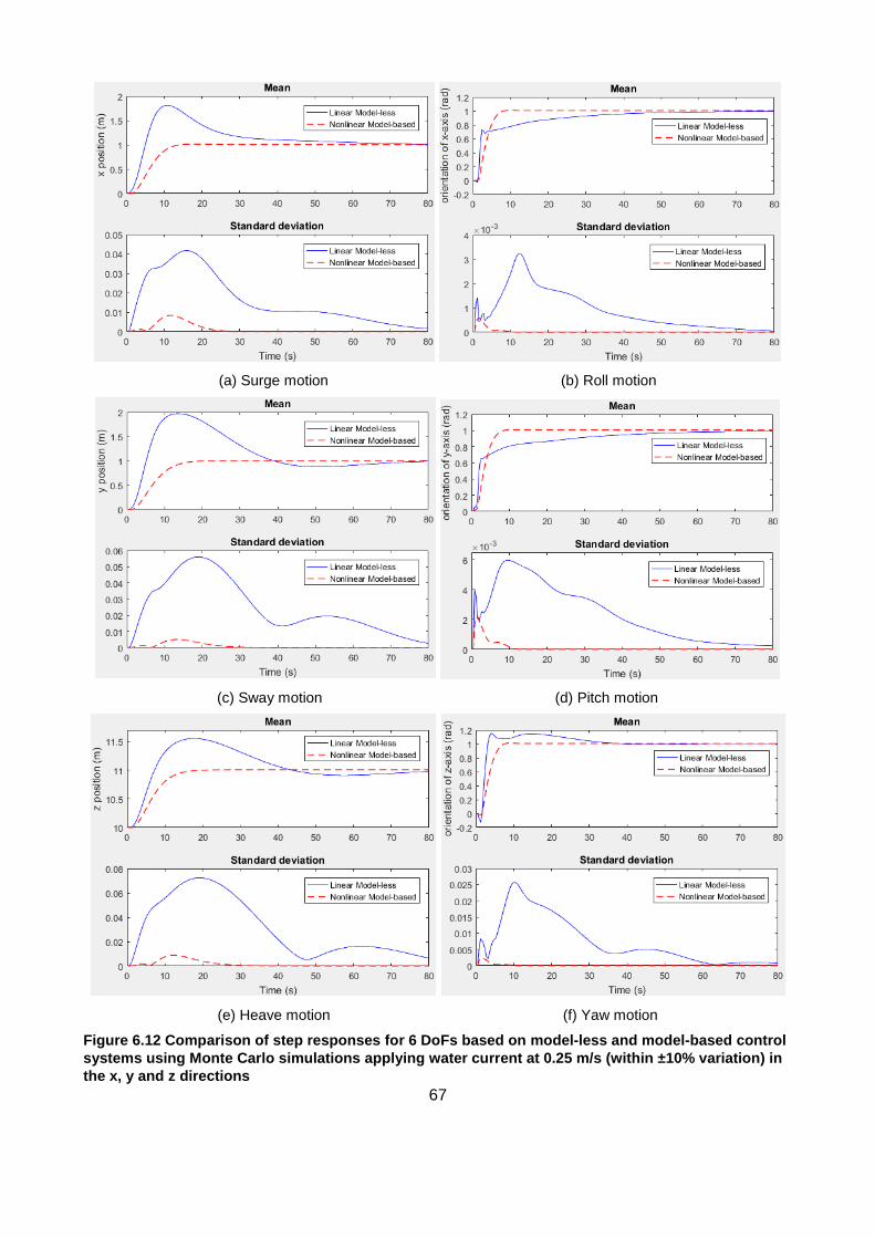
67
(a) Surge motion (b) Roll motion
(c) Sway motion (d) Pitch motion
(e) Heave motion (f) Yaw motion
Figure 6.12 Comparison of step responses for 6 DoFs based on model-less and model-based control
systems using Monte Carlo simulations applying water current at 0.25 m/s (within ±10% variation) in
the x, y and z directions
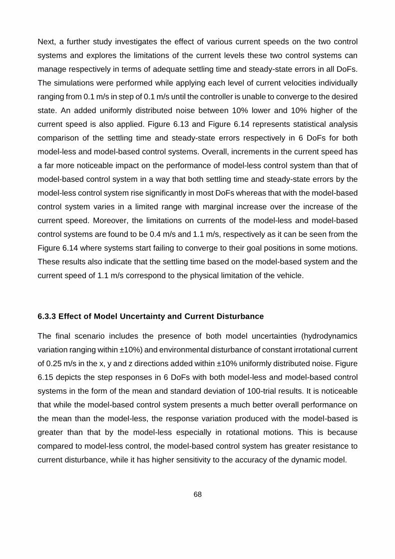
68
Next, a further study investigates the effect of various current speeds on the two control
systems and explores the limitations of the current levels these two control systems can
manage respectively in terms of adequate settling time and steady-state errors in all DoFs.
The simulations were performed while applying each level of current velocities individually
ranging from 0.1 m/s in step of 0.1 m/s until the controller is unable to converge to the desired
state. An added uniformly distributed noise between 10% lower and 10% higher of the
current speed is also applied. Figure 6.13 and Figure 6.14 represents statistical analysis
comparison of the settling time and steady-state errors respectively in 6 DoFs for both
model-less and model-based control systems. Overall, increments in the current speed has
a far more noticeable impact on the performance of model-less control system than that of
model-based control system in a way that both settling time and steady-state errors by the
model-less control system rise significantly in most DoFs whereas that with the model-based
control system varies in a limited range with marginal increase over the increase of the
current speed. Moreover, the limitations on currents of the model-less and model-based
control systems are found to be 0.4 m/s and 1.1 m/s, respectively as it can be seen from the
Figure 6.14 where systems start failing to converge to their goal positions in some motions.
These results also indicate that the settling time based on the model-based system and the
current speed of 1.1 m/s correspond to the physical limitation of the vehicle.
6.3.3 Effect of Model Uncertainty and Current Disturbance
The final scenario includes the presence of both model uncertainties (hydrodynamics
variation ranging within ±10%) and environmental disturbance of constant irrotational current
of 0.25 m/s in the x, y and z directions added within ±10% uniformly distributed noise. Figure
6.15 depicts the step responses in 6 DoFs with both model-less and model-based control
systems in the form of the mean and standard deviation of 100-trial results. It is noticeable
that while the model-based control system presents a much better overall performance on
the mean than the model-less, the response variation produced with the model-based is
greater than that by the model-less especially in rotational motions. This is because
compared to model-less control, the model-based control system has greater resistance to
current disturbance, while it has higher sensitivity to the accuracy of the dynamic model.
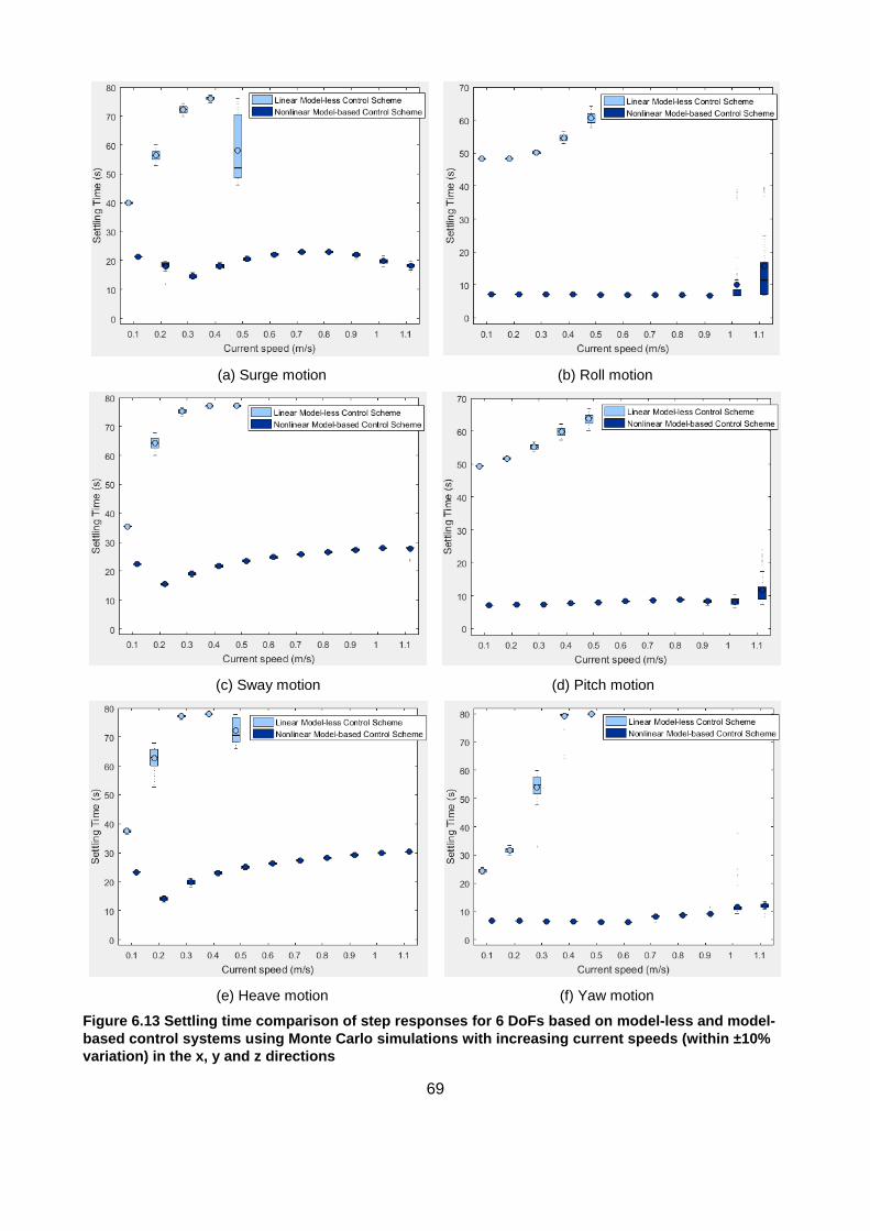
69
(a) Surge motion (b) Roll motion
(c) Sway motion (d) Pitch motion
(e) Heave motion (f) Yaw motion
Figure 6.13 Settling time comparison of step responses for 6 DoFs based on model-less and model-
based control systems using Monte Carlo simulations with increasing current speeds (within ±10%
variation) in the x, y and z directions
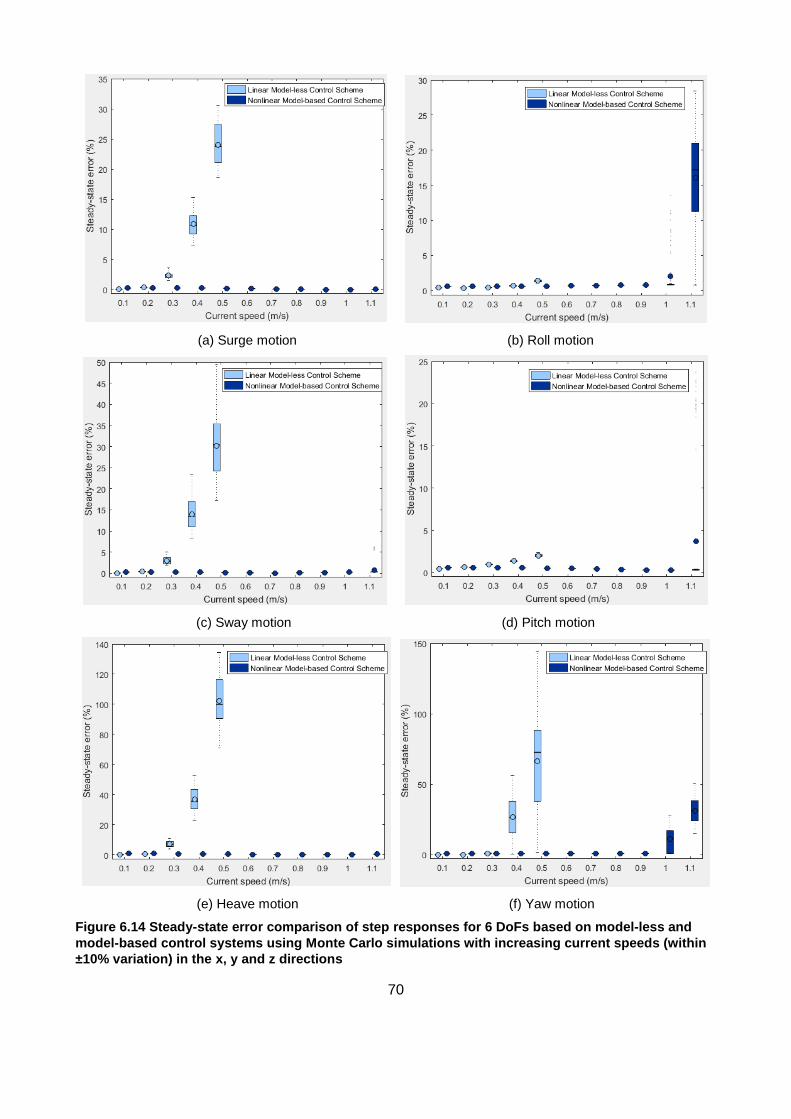
70
(a) Surge motion (b) Roll motion
(c) Sway motion (d) Pitch motion
(e) Heave motion (f) Yaw motion
Figure 6.14 Steady-state error comparison of step responses for 6 DoFs based on model-less and
model-based control systems using Monte Carlo simulations with increasing current speeds (within
±10% variation) in the x, y and z directions
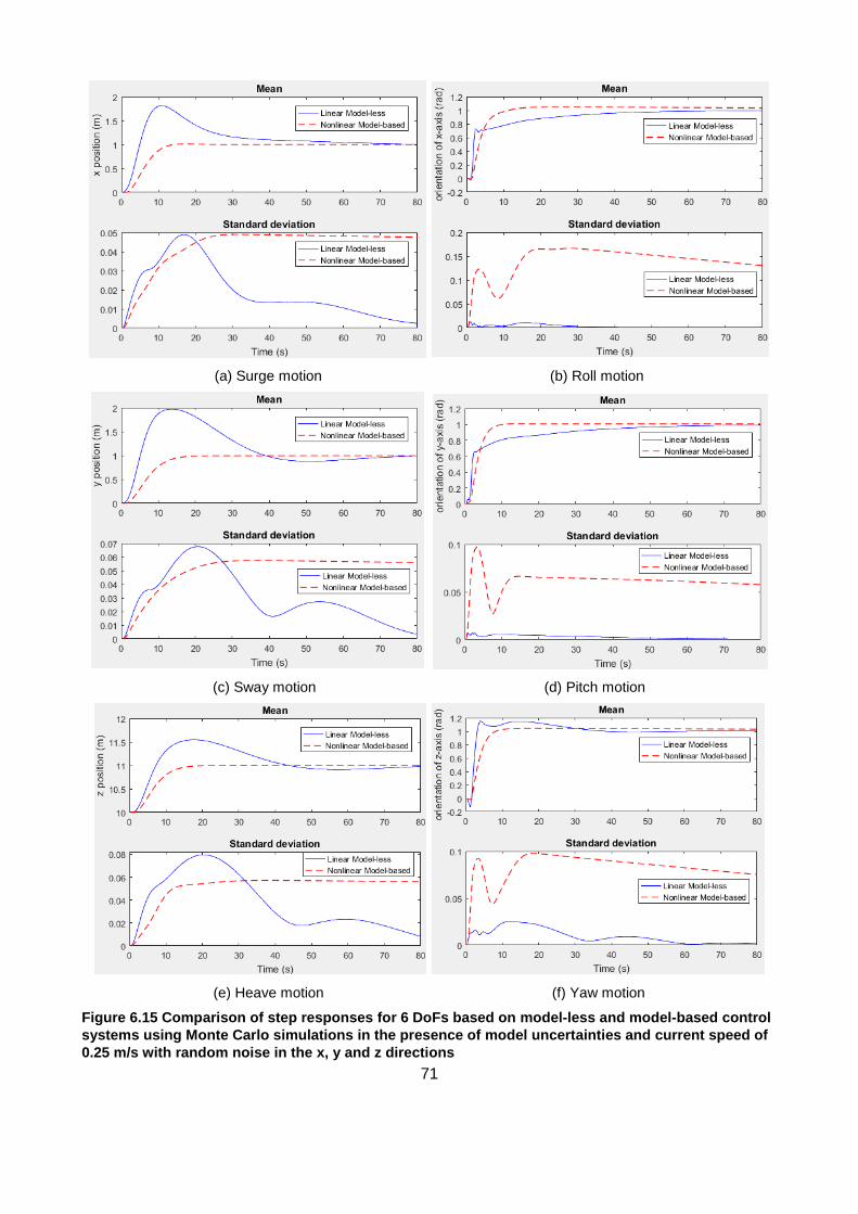
71
(a) Surge motion (b) Roll motion
(c) Sway motion (d) Pitch motion
(e) Heave motion (f) Yaw motion
Figure 6.15 Comparison of step responses for 6 DoFs based on model-less and model-based control
systems using Monte Carlo simulations in the presence of model uncertainties and current speed of
0.25 m/s with random noise in the x, y and z directions
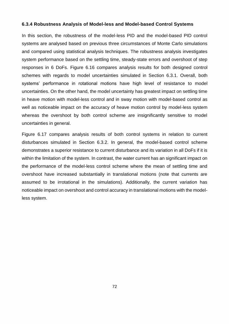
72
6.3.4 Robustness Analysis of Model-less and Model-based Control Systems
In this section, the robustness of the model-less PID and the model-based PID control
systems are analysed based on previous three circumstances of Monte Carlo simulations
and compared using statistical analysis techniques. The robustness analysis investigates
system performance based on the settling time, steady-state errors and overshoot of step
responses in 6 DoFs. Figure 6.16 compares analysis results for both designed control
schemes with regards to model uncertainties simulated in Section 6.3.1. Overall, both
systems’ performance in rotational motions have high level of resistance to model
uncertainties. On the other hand, the model uncertainty has greatest impact on settling time
in heave motion with model-less control and in sway motion with model-based control as
well as noticeable impact on the accuracy of heave motion control by model-less system
whereas the overshoot by both control scheme are insignificantly sensitive to model
uncertainties in general.
Figure 6.17 compares analysis results of both control systems in relation to current
disturbances simulated in Section 6.3.2. In general, the model-based control scheme
demonstrates a superior resistance to current disturbance and its variation in all DoFs if it is
within the limitation of the system. In contrast, the water current has an significant impact on
the performance of the model-less control scheme where the mean of settling time and
overshoot have increased substantially in translational motions (note that currents are
assumed to be irrotational in the simulations). Additionally, the current variation has
noticeable impact on overshoot and control accuracy in translational motions with the model-
less system.
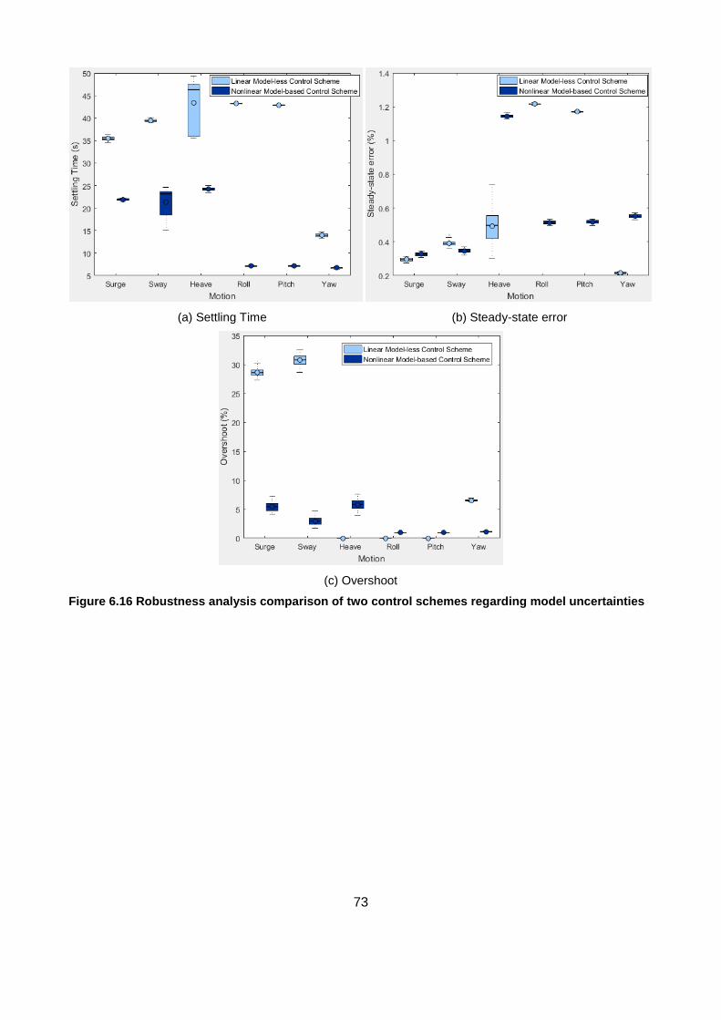
73
(a) Settling Time (b) Steady-state error
(c) Overshoot
Figure 6.16 Robustness analysis comparison of two control schemes regarding model uncertainties
74
(a) Settling Time (b) Steady-state error
(c) Overshoot
Figure 6.17 Robustness analysis comparison of two control schemes regarding current disturbance
Figure 6.18 compares analysis results of two control systems for the circumstance of both
model uncertainties and water currents simulated in Section 6.3.3. It can be seen that
although the mean performance in settling time and overshoot of the model-based control
is superior to that of the model-less control especially in translational motions, the accuracy
and settling time based on the model-based control in most DoFs varies in a larger but
acceptable range due to its sufficient resistance to current disturbance but reliance on the
model accuracy. To sum up, according to the analysis based on these three circumstances
of Monte Carlo simulations, the nonlinear model-based PID control system demonstrates an
effective and robust performance in relation to moderate model uncertainties and
environmental disturbance of currents whereas the linear model-less PID control scheme is
resistant to model uncertainties yet not providing sufficient performance in the presence of
current disturbance.
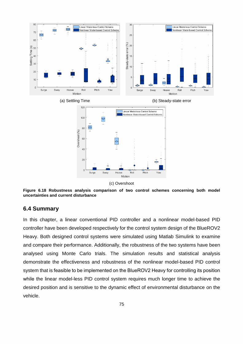
75
(a) Settling Time (b) Steady-state error
(c) Overshoot
Figure 6.18 Robustness analysis comparison of two control schemes concerning both model
uncertainties and current disturbance
6.4 Summary
In this chapter, a linear conventional PID controller and a nonlinear model-based PID
controller have been developed respectively for the control system design of the BlueROV2
Heavy. Both designed control systems were simulated using Matlab Simulink to examine
and compare their performance. Additionally, the robustness of the two systems have been
analysed using Monte Carlo trials. The simulation results and statistical analysis
demonstrate the effectiveness and robustness of the nonlinear model-based PID control
system that is feasible to be implemented on the BlueROV2 Heavy for controlling its position
while the linear model-less PID control system requires much longer time to achieve the
desired position and is sensitive to the dynamic effect of environmental disturbance on the
vehicle.
76
CHAPTER 7
CONCLUSION
7.1 Summary
This chapter will summarise the main components of the work achieved in this thesis and
present conclusions highlighting relevant findings and observations from simulation results.
Following this, recommendations of possible directions for future work will be presented.
The development of system modelling, identification and control systems for an ROV named
BlueROV2 Heavy have been presented in this thesis. In the first phase of this thesis, a
complete 6-DoF ROV’s system modelling was conducted using a vectorial representation
presented in Chapter 4. This includes the thruster model and the dynamic model of
kinematics and kinetics where various matrices that form the mathematical model were
derived on the basis of Fossen’s work (Fossen 1994, Fossen 2002, Fossen 2011). In order
to simplify the complex dynamic model and reduce the extensive unknown parameters,
several assumptions made for the BlueROV2 Heavy based on its characteristics and
relatively low speed operations were discussed in Section 3.3.
Inspired by the work of Indiveri (Indiveri 1998) and Caccia (Caccia, Indiveri et al. 2000), a
system identification approach in immersion tank with the use of on-board sensors was
proposed in Section 5.1 for determining parameters in the dynamic model. This approach
employs static experiments for identifying damping parameters where the velocity of the
vehicle is constant and the acceleration is zero; and utilises dynamic experiments for
identifying system inertia parameters where the acceleration of the vehicle is non-zero. This
approach is highly repeatable and cost effective, which makes it suited for the BlueROV2
Heavy as the vehicle is easily configurable and fully customisable. The bollard pull test in
immersion tank with the use of a 6-DoF load cell was proposed in Section 5.3 for identifying
thruster coefficients in the thruster model. Using an estimation technique of the least squares
algorithm to estimate parameters from the experimental data was demonstrated in Section
5.1.1. However, due to the unavailability of the BlueROV2 Heavy, system identification
experiments were not carried out. Alternatively, parameters in the models were determined
by analysing the BlueROV2 Heavy’s technical specifications from BlueRobotics
77
(BlueRobotics 2018b) and published literature relating to BlueROV from Sandøy (Sandøy
2016) presented in Section 5.2 and 5.3.
In the second phase of this thesis, a simulation study of the control system design was
presented, with the use of the system model and parameters determined for the BlueROV2
Heavy, in Chapter 6. Various controller algorithms applicable to an underwater vehicle were
discussed in detail, as presented in Section 2.2. Two 6-DoF control systems of linear model-
less and nonlinear model-based were developed for the vehicle based upon the PID control
algorithm presented in Section 6.1 due to its simplicity, practicability and ease of
implementation. Step response of each DoF and path following simulations using these two
control systems as well as result analysis and their performance comparison were presented
in Section 6.2. Section 6.3 presented the results and analysis of a set of representative
Monte Carlo simulations under various operating conditions in order to investigate the
robustness of these two control systems. Three scenarios were set as in the presence of
the model uncertainty, the current disturbance and the combination of the two. These
simulation results were analysed based on the mean and standard deviation of the step
responses for all DoFs based on 100 trials. Using statistical analysis and representation of
boxplots, the robustness of two systems were examined and compared for control
performance and accuracy.
7.2 Conclusions
Based on the work presented in this thesis, several conclusions can be drawn regarding the
findings from the simulation studies. These conclusions are concerned with the performance
of the two developed control systems in relation to settling time, steady-state error,
overshoot and robustness to environmental disturbances and model uncertainties.
In the first simulation study of step response and path following simulations, it was seen that
both the 6-DoF linear model-less PID and the 6-DoF nonlinear model-based PID control
systems were able to track a simple trajectory (i.e. a single DoF is excited at a time) in all 6
DoFs without external disturbances. Although the technique of the linear conventional PID
controller is relatively simple to implement, it produces long settling time for certain DoFs
(about 50 secs in heave, roll and pitch) and noticeable overshoot in surge and sway motions
78
(about 30%). Furthermore, due to the highly nonlinear properties of the ROV’s model, linear
control schemes are incapable of producing sufficient manoeuvring performance in the
presence of current disturbance from the external environment. The nonlinear model-based
PID control system was formed by extending the PID controller with the concept of model-
based control. In this design, the vehicle’s dynamic model is taken advantage of to produce
a predictive force and the PID controller is utilised to provide a corrective force for the
residual error. As a result, the model-based control system has at least 42% of improvement
in settling time and at least 62% of improvement in overshoot with 138% longer processing
time whereas both systems are fast enough for implementation (i.e. the maximum updated
rate for model-less and model-based control systems are 1.5 kHz and 640 Hz while a control
system generally require processing speed of 100 Hz).
In the second simulation study of robustness analysis using Monte Carlo simulations, it was
found that both model-less and model-based control systems are relatively insensitive (with
1.5% change) to the model uncertainty (with a ±10% variation in hydrodynamic parameters)
in most DoFs (especially in rotational motions). The noticeable impacts of the model
uncertainty were found to be on settling time in heave motion (greatest) and on steady-state
error on heave motion with the model-less control; and on settling time in sway motion with
the model-based control. In the presence of current disturbance, the model-based control
demonstrates a superior robustness whereas the average settling time and overshoot have
increased substantially in translational motions (currents were assumed to be irrotational)
with the model-less control. The operational limits regarding current disturbance for model-
less and model-based control were found to be current speed of 0.4 m/s and 1.1 m/s,
respectively. For the scenario of both model uncertainties and water currents, the overall
performance in settling time and overshoot of the model-based control is superior to that of
the model-less control due to its sufficient resistance to current disturbance. However, since
the model-based control relies on the accuracy of the model to a certain degree, the
performance of settling time and steady-state error varies in a larger range compared with
the model-less control. According to the statistical analysis of simulation results based on
these three scenarios, the nonlinear model-based PID control system was validated to be
robust with regards to moderate model uncertainties (±10% variation in hydrodynamic
parameters) and current disturbance up to 1.1 m/s current speed whereas the linear model-
79
less PID control system less insensitive to model uncertainties yet not capable of handling
disturbances and only effective for a relatively small range from the tuning point.
7.3 Recommendations for Future Work
This section presents a summary of intended and possible work that could be undertaken
to increase the accuracy of system identification and expand the functionality of the control
system.
7.3.1 Improvement of System Identification
In this thesis, the unknown parameters in the derived models of BlueROV2 Heavy were
currently determined by analysing technical specifications and published literature relating
to BlueROV that could potentially have significant inaccuracy due to the effects of
hydrodynamic, thruster-hull and thruster-thruster interactions, and different configuration of
BlueROV. Therefore, once the BlueROV2 Heavy is available, it is essential to perform the
system identification experiments for higher accuracy in identifying parameters.
The proposed system identification approach exploits the characteristics of the ROV and
assumes decoupling between DoFs in hydrodynamics. As a consequence, hydrodynamic
parameters for each DoF can be estimated independently with the use of the vehicle’s state
measurements obtained by on-board sensors. Under the consideration of measurement
noise from on-board sensors, a state observer algorithm is then necessary to process the
available measurements to attain an estimate of the position and velocity of the vehicle with
minimal noise corrupting the solution. This estimated information from the observer can be
also utilised in the state feedback control. This can be achieved by employing a recursive
Bayesian filtering technique, which comprises the Kalman filter family and the particle filter
family. Due to the highly nonlinear dynamic properties of the ROV, a nonlinear observer
such as an Extended Kalman Filter (EKF) or non-Gaussian filtering of the particle filter can
be chosen for their ease of implementation. The implementation examples for the EKF and
the particle filter for ROV’s observer can be found in literature of Dukan et al. (Dukan,
Ludvigsen et al. 2011) and Zhao et al. (Zhao, Skjetne et al. 2014), respectively.
80
While various assumptions were placed on the vehicle to simplify its 6-DoF model and
reduce the number of unknown parameters in the model, the accuracy of the obtained model
might be decreased due to accumulated approximations. Therefore, relaxation of
assumptions improves the accuracy of the ROV’s model and ultimately leads to a more
robust control system. In the kinetic equation of motion, the system inertia and hydrostatic
terms can be attained by measuring, which are relatively accurate. However, the damping
terms of hydrodynamics are depending on motion of fluid surrounding the vehicle and
sensitive to the velocity that are challenging to obtain accurately. Hence, it is recommended
to incorporate significant off-diagonal parameters of damping matrices to minimise
assumptions and increase accuracy. Note that determining which off-diagonal terms are
significant needs to be investigated in the future by utilising data from experiments.
7.3.2 Improvement of Controller
In the control system design, the gains of the PID controllers for both designed systems will
need to be refined when model parameters for the BlueROV2 Heavy are updated and
obtained from experimental system identification to attain optimal values. The developed
control systems in this thesis concern position control of the vehicle for ROV’s inspection
and intervention purposes. The next stage is to include speed control to expand system
capacity for surveying and mapping by integrating a desired velocity and the estimated state
of velocity into the control system. This can be realised by applying a common technique
used in robotics named computed torque control (Scıavıcco and Siciliano 1996). This
approach conducts state feedback linearisation that utilises a nonlinear mapping to
transform the nonlinear system dynamics into a linear system. The examples of
implementation of this approach for underwater vehicles can be found in literature (Silpa-
Anan, Abdallah et al. 2000, Smallwood and Whitcomb 2004).
As existing control solutions reported in the literature review presented in Chapter 2, the PID
controller is one of the control algorithms for underwater vehicles. The modern control
technique of sliding mode control is becoming increasingly used due to its relatively simple
implementation (Marco and Healey 2001) and insensitivity to model uncertainties and
external disturbances and has been demonstrated to achieve robust control (Gomes, Sousa
et al. 2003, Soylu, Buckham et al. 2008, Haugen 2012). However, a particular limitation of
81
the conventional sliding mode control is the phenomenon of chattering, which is a high
frequency oscillation introduced by the discontinuity in the control law. This oscillation can
lead to unmodelled dynamics, excessive power consumption and system instability.
Nevertheless, the chattering effect of sliding model control can be reduced by introducing a
boundary layer around the sliding surface by applying saturation function (Slotine and Li
1991) or the sigmoid function (Edwards and Spurgeon 1998) under a continuous control
law. Alternatively, another chattering elimination method is using higher order sliding modes
to hide control discontinuity in its higher derivatives (Fridman and Levant 1996, Bartolini,
Ferrara et al. 1998).This approach has been realised in literature presenting enhanced
accuracy and robustness to external disturbances. Since sliding mode control can produce
more accurate solution and has an equivalent computation load to model-based PID control,
it is recommended for future development.
7.4 Epilogue
In summarising this thesis, it can be seen, through representative and quantitative
simulations, that a 6-DoF control system utilising model-based control framework provides
accurate and robust control performance compared with the linear conventional controller.
While both developed control systems have satisfactory computation time for
implementation, simulation results demonstrate significant performance improvement (i.e.
at least 42% settling time reduction and at least 62% overshoot reduction) by the nonlinear
model-based control (with the cost of 138% more processing time). Furthermore, it was seen
that the nonlinear model-based control responses to dynamic effects of disturbances on the
system efficiently and has a much larger operational range (up to 1.1 m/s current speed
compared with up to 0.4 m/s current speed for model-less control). To conclude, from this
thesis it is evident that the developed 6-DoF nonlinear model-based PID control system is
feasible to be implemented in controlling the position of the BlueROV2 Heavy in all 6 DoFs.
82
Bibliography
Abkowitz, M. A. (1964). Lectures on ship hydrodynamics--Steering and manoeuvrability.
Abkowitz, M. A. (1980). Measurement of hydrodynamic characteristics from ship maneuvering trials by system identification.
Aili, A. and E. Ekelund (2016). Model-Based Design, Development and Control of an Underwater Vehicle.
Alessandri, A., et al. (1998). Application of LS and EKF techniques to the identification of underwater vehicles. Control Applications, 1998. Proceedings of the 1998 IEEE International Conference on, IEEE.
Alvarez, A., et al. (2009). "Folaga: A low-cost autonomous underwater vehicle combining glider and AUV capabilities." Ocean Engineering 36(1): 24-38.
Amado-Filho, G. M., et al. (2012). "Occurrence and distribution of rhodolith beds on the Fernando de Noronha Archipelago of Brazil." Aquatic botany 101: 41-45.
Antonelli, G., et al. (2001). "Adaptive control of an autonomous underwater vehicle: experimental results on ODIN." IEEE Transactions on Control Systems Technology 9(5): 756-765.
Arnesen, B. O. (2016). Motion Control Systems for ROVs-Underwater Path-Following for a Videoray Pro 4 ROV, NTNU.
Åström, K. J. and T. Hägglund (1995). PID controllers: theory, design, and tuning, Instrument society of America Research Triangle Park, NC.
Åström, K. J. and T. Hägglund (2006). Advanced PID control. The Instrumentation, Systems, and Automation Society, Citeseer.
Bachmayer, R. and L. L. Whitcomb (2003). "Adaptive parameter identification of an accurate nonlinear dynamical model for marine thrusters." TRANSACTIONS-AMERICAN SOCIETY OF MECHANICAL ENGINEERS JOURNAL OF DYNAMIC SYSTEMS MEASUREMENT AND CONTROL 125(3): 491-493.
Bartolini, G., et al. (1998). "Chattering avoidance by second-order sliding mode control." IEEE Transactions on Automatic control 43(2): 241-246.
Berge, S. and T. Fossen (2000). "On the properties of the nonlinear ship equations of motion." Mathematical and Computer Modelling of Dynamical Systems 6(4): 365-381.
83
Bessa, W. M., et al. (2010). "An adaptive fuzzy sliding mode controller for remotely operated underwater vehicles." Robotics and Autonomous Systems 58(1): 16-26.
Blanke, M., et al. (2000). "Dynamic model for thrust generation of marine propellers." IFAC Proceedings Volumes 33(21): 353-358.
BlueRobotics (2017). from https://www.bluerobotics.com/store/rov/bluerov2/.
BlueRobotics (2018a). "BlueROV2 Heavy Configuration Retrofit Kit." from https://www.bluerobotics.com/store/rov/brov2-heavy-retrofit-r1-rp/.
BlueRobotics (2018b). "BlueROV2 Heavy Retrofit Documentation." from http://docs.bluerobotics.com/brov2-heavy/.
BlueRobotics (2018c). "T200 Thruster." from https://www.bluerobotics.com/store/thrusters/t200-thruster/.
Caccia, M., et al. (2000). "Modeling and identification of open-frame variable configuration unmanned underwater vehicles." IEEE Journal of Oceanic Engineering 25(2): 227-240.
Caccia, M. and G. Veruggio (2000). "Guidance and control of a reconfigurable unmanned underwater vehicle." Control engineering practice 8(1): 21-37.
Capocci, R., et al. (2017). "Inspection-Class Remotely Operated Vehicles—A Review." Journal of Marine Science and Engineering 5(1): 13.
Chalkiadakis, V., et al. (2017). Designing a small-sized autonomous underwater vehicle architecture for regular periodic fish-cage net inspection. Imaging Systems and Techniques (IST), 2017 IEEE International Conference on, IEEE.
Chen, H.-H., et al. (2007). Identification of hydrodynamic parameters for a remotely operated vehicle using projective mapping method. Underwater Technology and Workshop on Scientific Use of Submarine Cables and Related Technologies, 2007. Symposium on, IEEE.
Chin, C., et al. (2017). "Experimental validation of open-frame ROV model for virtual reality simulation and control." Journal of Marine Science and Technology: 1-21.
Chou, J. C. (1992). "Quaternion kinematic and dynamic differential equations." IEEE transactions on robotics and automation 8(1): 53-64.
Christ, D. and L. Wernli (2007). "TheROv Manual: A User Guide for Observation Class Remotely Operated Vehicles."
84
Chu, Z., et al. (2017). "Observer-based adaptive neural network trajectory tracking control for remotely operated vehicle." IEEE transactions on neural networks and learning systems 28(7): 1633-1645.
Cristi, R., et al. (1990). "Adaptive sliding mode control of autonomous underwater vehicles in the dive plane." IEEE Journal of Oceanic Engineering 15(3): 152-160.
de Barros, E. A., et al. (2008). "Investigation of normal force and moment coefficients for an AUV at nonlinear angle of attack and sideslip range." IEEE Journal of Oceanic Engineering 33(4): 538-549.
Do, K. D., et al. (2004). "Robust and adaptive path following for underactuated autonomous underwater vehicles." Ocean Engineering 31(16): 1967-1997.
Dukan, F. (2014). "Rov motion control systems."
Dukan, F., et al. (2011). Dynamic positioning system for a small size ROV with experimental results. OCEANS, 2011 IEEE-Spain, IEEE.
Edwards, C. and S. Spurgeon (1998). Sliding mode control: theory and applications, Crc Press.
Egeland, O. and J. T. Gravdahl (2002). Modeling and simulation for automatic control, Marine Cybernetics Trondheim, Norway.
Eidsvik, O. A. (2015). Identification of hydrodynamic parameters for remotely operated vehicles, NTNU.
Eng, Y.-H., et al. (2014). "Added mass computation for control of an open-frame remotely-operated vehicle: Application using WAMIT and MATLAB." Journal of Marine Science and Technology 22(4): 405-416.
Eng, Y., et al. (2008). Identification of the hydrodynamics coefficients of an underwater vehicle using free decay pendulum motion. International MultiConference of Engineers and Computer Scientists.
Erikson, U., et al. (2016). "Crowding of Atlantic salmon in net-pen before slaughter." Aquaculture 465: 395-400.
Faltinsen, O. (1990). "Sea loads on ships and ocean structures." Cambridge University, Cambridge, UK.
Fernandes, D. d. A., et al. (2013). "Trajectory tracking motion control system for observation class ROVs." IFAC Proceedings Volumes 46(33): 251-256.
85
Fernandes, D. d. A., et al. (2015). "Output feedback motion control system for observation class ROVs based on a high-gain state observer: Theoretical and experimental results." Control engineering practice 39: 90-102.
Fossen, T. I. (1991). Nonlinear modelling and control of underwater vehicles, Fakultet for informasjonsteknologi, matematikk og elektroteknikk.
Fossen, T. I. (1994). Guidance and control of ocean vehicles, John Wiley & Sons Inc.
Fossen, T. I. (2002). Marine control systems: guidance, navigation and control of ships, rigs and underwater vehicles, Marine Cybernetics.
Fossen, T. I. (2011). Handbook of marine craft hydrodynamics and motion control, John Wiley & Sons.
Fossen, T. I. and T. A. Johansen (2006). A survey of control allocation methods for ships and underwater vehicles. Control and Automation, 2006. MED'06. 14th Mediterranean Conference on, IEEE.
Franklin, G. F., et al. (1994). Feedback control of dynamic systems, Addison-Wesley Reading, MA.
Fridman, L. and A. Levant (1996). Higher order sliding modes as a natural phenomenon in control theory. Robust Control via variable structure and Lyapunov techniques, Springer: 107-133.
Goheen, K. and E. Jefferys (1990). The application of alternative modelling techniques to ROV dynamics. Robotics and Automation, 1990. Proceedings., 1990 IEEE International Conference on, IEEE.
Goheen, K. R. (1986). The modelling and control of remotely operated underwater vehicles, University of London.
Goheen, K. R. and E. R. Jefferys (1990). "Multivariable self-tuning autopilots for autonomous and remotely operated underwater vehicles." IEEE Journal of Oceanic Engineering 15(3): 144-151.
Goldstein, H. (1980). Classical mechanics, Pearson Education India.
Gomes, R. M., et al. (2003). Modeling and control of the IES project ROV. European Control Conference (ECC), 2003, IEEE.
Gonzalez, L. A. (2004). "Design, modelling and control of an autonomous underwater vehicle." Bachelor of Engineering Honours Thesis. The University of Western Australia.
Goodman, A. (1960). Experimental techniques and methods of analysis used in submerged body research. Proceedings of the Third Symposium on Naval Hydrodynamics, National Academy Press.
86
Haugen, M. (2012). Modeling and Control of ROV Manipulator, Institutt for marin teknikk.
Healey, A. J. and D. Lienard (1993). "Multivariable sliding mode control for autonomous diving and steering of unmanned underwater vehicles." IEEE Journal of Oceanic Engineering 18(3): 327-339.
Healey, A. J., et al. (1994). Toward an improved understanding of thruster dynamics for underwater vehicles. Autonomous Underwater Vehicle Technology, 1994. AUV'94., Proceedings of the 1994 Symposium on, IEEE.
Hoang, N. Q. and E. Kreuzer (2007). "Adaptive PD-controller for positioning of a remotely operated vehicle close to an underwater structure: Theory and experiments." Control engineering practice 15(4): 411-419.
Hsu, L., et al. (2000). "Dynamic positioning of remotely operated underwater vehicles." IEEE Robotics & Automation Magazine 7(3): 21-31.
Huang, H.-M. (2004). "Autonomy levels for unmanned systems (ALFUS) framework volume I: Terminology version 2.0." Special Publication (NIST SP)-1011.
Hughes, P. C. (1986). "Spacecraft Attitude Dynamics John Wiley and Sons." New York.
Humphreys, D. and K. Watkinson (1982). "Hydrodynamic stability and control analyses of the UNH-EAVE autonomous underwater vehicle." Marine Systems Lab. Rep., Univ. of New Hamp., Durham.
Indiveri, G. (1998). "Modelling and identification of underwater robotic systems." Computer Science.
Jakobsen, R. A. H. (2011). Automatic Inspection of Cage Integrity with Underwater Vehicle, Institutt for teknisk kybernetikk.
Javadi-Moghaddam, J. and A. Bagheri (2010). "An adaptive neuro-fuzzy sliding mode based genetic algorithm control system for under water remotely operated vehicle." Expert Systems with Applications 37(1): 647-660.
Juul, D. L., et al. (1994). Submersible control using the linear quadratic gaussian with loop transfer recovery method. Autonomous Underwater Vehicle Technology, 1994. AUV'94., Proceedings of the 1994 Symposium on, IEEE.
Kalske, S. (1989). Motion dynamics of subsea vehicles, Espoo.
Kane, T. R., et al. (1983). "Spacecraft dynamics." New York, McGraw-Hill Book Co, 1983, 445 p.
87
Kim, J. and W. K. Chung (2006). "Accurate and practical thruster modeling for underwater vehicles." Ocean Engineering 33(5-6): 566-586.
Kodogiannis, V., et al. (1996). "Neural network modelling and control for underwater vehicles." Artificial intelligence in Engineering 10(3): 203-212.
Lapierre, L., et al. (2003). Nonlinear path following with applications to the control of autonomous underwater vehicles. Decision and Control, 2003. Proceedings. 42nd IEEE Conference on, IEEE.
Lewis, D., et al. (1984). "The simulation of remotely operated underwater vehicles." Proceedings, ROV'84: 245-252.
Li, Z., et al. (2012). "Robust adaptive motion control for underwater remotely operated vehicles with velocity constraints." International Journal of Control, Automation and Systems 10(2): 421-429.
Liu, G. (1993). "Application of EKF technique to ship resistance measurement." Automatica 29(2): 275-283.
Mai, C., et al. (2017). "Modeling and Control of Industrial ROV’s for Semi-Autonomous Subsea Maintenance Services." IFAC-PapersOnLine 50(1): 13686-13691.
Marco, D. B. and A. Healey (1998). "Surge motion parameter identification for the NPS Phoenix AUV."
Marco, D. B. and A. J. Healey (2001). "Command, control, and navigation experimental results with the NPS ARIES AUV." IEEE Journal of Oceanic Engineering 26(4): 466-476.
Marsh, L., et al. (2013). "Getting the bigger picture: using precision Remotely Operated Vehicle (ROV) videography to acquire high-definition mosaic images of newly discovered hydrothermal vents in the Southern Ocean." Deep Sea Research Part II: Topical Studies in Oceanography 92: 124-135.
Meirovitch, L. (1990). Dynamics and control of structures, John Wiley & Sons.
Mills, D. and C. Harris (1995). "Neurofuzzy modelling and control of a six degree of freedom AUV." Research Journal Image, Speech and Intelligent Systems.
Minorsky, N. (1922). "Directional stability of automatically steered bodies." Journal of ASNE 42(2): 280-309.
Morrison, A. and D. R. Yoerger (1993). Determination of the hydrodynamic parameters of an underwater vehicle during small scale, nonuniform, 1-dimensional translation. OCEANS'93. Engineering in Harmony with Ocean. Proceedings, IEEE.
88
Naeem, W., et al. (2003). "LQG/LTR control of an autonomous underwater vehicle using a hybrid guidance law." IFAC Proceedings Volumes 36(4): 31-36.
NationalOceanographyCentre (2018). "Isis Deep ROV Platform." from http://www.noc.ac.uk/facilities/marine-autonomous-robotic-systems/deep-platforms.
Newman, J. "Marine hydrodynamics, 1977." Massachusetts Institute of Technology, Cambridge, Massachusetts). Google Scholar: 19.
Nomoto, M. and M. Hattori (1986). "A deep ROV" DOLPHIN 3K": design and performance analysis." IEEE Journal of Oceanic Engineering 11(3): 373-391.
NTNU (2018). "ROV Minerva." from https://www.ntnu.edu/oceans/minerva.
OceanExplorationTrust (2003). "ROV Hercules." from http://www.oceanexplorationtrust.org/remotely-operated-vehicles.
Perrier, M. and C. Canudas-De-Wit (1996). Experimental comparison of PID vs. PID plus nonlinear controller for subsea robots. Underwater Robots, Springer: 121-138.
Quigley, M., et al. (2009). ROS: an open-source Robot Operating System. ICRA workshop on open source software, Kobe, Japan.
Raimondi, F. M. and M. Melluso (2010). "Fuzzy/Kalman hierarchical horizontal motion control of underactuated ROVs." International Journal of Advanced Robotic Systems 7(2): 12.
Raptis, I. A. (2010). Linear and nonlinear control of unmanned rotorcraft, University of South Florida.
Ridao, P., et al. (2004). "On the identification of non-linear models of unmanned underwater vehicles." Control engineering practice 12(12): 1483-1499.
Rist-Christensen, I. (2016). Autonomous robotic intervention using ROV, NTNU.
Roman, C., et al. (2010). Application of structured light imaging for high resolution mapping of underwater archaeological sites. OCEANS 2010 IEEE-Sydney, IEEE.
Ross, A., et al. (2004). "Identification of underwater vehicle hydrodynamic coefficients using free decay tests." IFAC Proceedings Volumes 37(10): 363-368.
SAAB (2002). "Seaeye Falcon & Seaeye Falcon DR." from http://www.seaeye.com/falcon.html.
Sandøy, S. S. (2016). System Identification and State Estimation for ROV uDrone, NTNU.
89
Sargent, J. S. and P. N. Cowgill (1976). Design considerations for dynamically positioned utility vessels. Offshore Technology Conference, Offshore Technology Conference.
Sarkar, T., et al. (1997). "A study of autonomous underwater vehicle hull forms using computational fluid dynamics." International Journal for Numerical Methods in Fluids 25(11): 1301-1313.
Sarpkaya, T. and M. Isaacson (1981). "Mechanics of wave forces on offshore structures."
Sayyaadi, H. and T. Ura (1999). Multi input-multi output system identification of AUV systems by neural network. OCEANS'99 MTS/IEEE. Riding the Crest into the 21st Century, IEEE.
Scıavıcco, L. and B. Siciliano (1996). Modeling and control of robot manipulators, The McGraw-Hill Companies, New York.
Sebastián, E. and M. A. Sotelo (2007). "Adaptive fuzzy sliding mode controller for the kinematic variables of an underwater vehicle." Journal of Intelligent and Robotic Systems 49(2): 189-215.
Sedlazeck, A., et al. (2009). 3d reconstruction based on underwater video from rov kiel 6000 considering underwater imaging conditions. OCEANS 2009-EUROPE, IEEE.
Silpa-Anan, C., et al. (2000). Development of autonomous underwater vehicle towards visual servo control. Proceedings of the Australian Conference on Robotics and Automation. Melbourne, Australia.
Singh, H., et al. (2007). "Towards high-resolution imaging from underwater vehicles." The International journal of robotics research 26(1): 55-74.
Slotine, J.-J. and S. S. Sastry (1983). "Tracking control of non-linear systems using sliding surfaces, with application to robot manipulators." International journal of control 38(2): 465-492.
Slotine, J.-J. E. and W. Li (1991). Applied nonlinear control, Prentice hall Englewood Cliffs, NJ.
Smallwood, D. A. and L. L. Whitcomb (2003). "Adaptive identification of dynamically positioned underwater robotic vehicles." IEEE Transactions on Control Systems Technology 11(4): 505-515.
Smallwood, D. A. and L. L. Whitcomb (2004). "Model-based dynamic positioning of underwater robotic vehicles: theory and experiment." IEEE Journal of Oceanic Engineering 29(1): 169-186.
SNAME (1950). "Nomenclature for treating the motion of a submerged body through a fluid JR." New York: Technical and Research Bulletin: 1-5.
90
Song, F. and S. M. Smith (2000). Design of sliding mode fuzzy controllers for an autonomous underwater vehicle without system model. Oceans 2000 MTS/IEEE Conference and Exhibition, IEEE.
Sørensen, A. J. (2012). "Marine control systems propulsion and motion control of ships and ocean structures lecture notes."
Soylu, S., et al. (2008). "A chattering-free sliding-mode controller for underwater vehicles with fault-tolerant infinity-norm thrust allocation." Ocean Engineering 35(16): 1647-1659.
SPERRE (2012). "SUB-FIGHTER 30K." from http://sperre-as.com/portfolio/sub-fighter-30k/.
Strand, J. P. (1999). "Nonlinear Position Control Systems Gesign for Marine Yessels."
Sun, Y. and C. Cheah (2003). Adaptive setpoint control for autonomous underwater vehicles. Decision and Control, 2003. Proceedings. 42nd IEEE Conference on, IEEE.
Svendby, E. (2007). Robust control of ROV/AUVs, Institutt for teknisk kybernetikk.
Triantafyllou, M. S. and F. S. Hover (2003). Maneuvering and control of marine vehicles, Massachusetts of Institute of Technologyq.
Utkin, V. (1977). "Variable structure systems with sliding modes." IEEE Transactions on Automatic control 22(2): 212-222.
VideoRay (2018a). "Pro 3 ROV Image Gallery." from http://www.videoray.com/pro-3-rov-photo-gallery.html#!RigWorkerGTO_sm.
VideoRay (2018b). "VideoRay Explorer ROV Images." from http://www.videoray.com/explorer-rov-photo-gallery.html#!Explorer_Display_sm.
VideoRay (2018c). "VideoRay Pro 4 ROV Images." from http://www.videoray.com/videoray-pro-4-photo-gallery.html#!_SRC1370_sm.
Wahl, A. and E. Gilles (1999). Model predictive versus linear quadratic control for the tracking problem of automatic river navigation. Control Conference (ECC), 1999 European, IEEE.
Walther, D., et al. (2004). Detection and tracking of objects in underwater video. Computer Vision and Pattern Recognition, 2004. CVPR 2004. Proceedings of the 2004 IEEE Computer Society Conference on, IEEE.
Wang, J.-S. and C. G. Lee (2003). "Self-adaptive recurrent neuro-fuzzy control of an autonomous underwater vehicle." IEEE transactions on robotics and automation 19(2): 283-295.
91
Whitcomb, L. L. and D. R. Yoerger (1999). "Development, comparison, and preliminary experimental validation of nonlinear dynamic thruster models." IEEE Journal of Oceanic Engineering 24(4): 481-494.
Yahya, M. and M. Arshad (2016). Position-based visual servoing for underwater docking of an autonomous underwater vehicle. Underwater System Technology: Theory and Applications (USYS), IEEE International Conference on, IEEE.
Yi, D. and H. Al-Qrimli (2017). "Identification of Hydrodynamics Coefficient of Underwater Vehicle Using Free Decay Pendulum Method." J Powder Metall Min 6(161): 2.
Yoerger, D. and J. Slotine (1985). "Robust trajectory control of underwater vehicles." IEEE Journal of Oceanic Engineering 10(4): 462-470.
Yoerger, D. R., et al. (1990). "The influence of thruster dynamics on underwater vehicle behavior and their incorporation into control system design." IEEE Journal of Oceanic Engineering 15(3): 167-178.
Yuh, J. (1990). "Modeling and control of underwater robotic vehicles." IEEE Transactions on Systems, man, and Cybernetics 20(6): 1475-1483.
Zhang, H., et al. (2010). "Using CFD software to calculate hydrodynamic coefficients." Journal of Marine Science and Application 9(2): 149-155.
Zhao, B., et al. (2014). "Particle filter for fault diagnosis and robust navigation of underwater robot." IEEE Transactions on Control Systems Technology 22(6): 2399-2407.
Ziegler, J. G. and N. B. Nichols (1942). "Optimum settings for automatic controllers." trans. ASME 64(11).