The controllability of the Gurtin-Pipkin

equation:

a cosine operator approach

Luciano Pandolfi∗

Politecnico di Torino, Dipartimento di Matematica,Corso Duca degli Abruzzi 24, 10129 Torino — Italy,

Tel. +39-11-5647516 luciano.pandolfi@polito.it

October 17, 2011

Author version. Paper published in Applied Mathematicsand Optimization Appl Mat Optim (2005) 52: 143-165, DOI:10.1007/s00245-005-0819-0

AbstractIn this paper we give a semigroup-based definition of the solution

of the Gurtin-Pipkin equation with Dirichlet boundary conditions. Itturns out that the dominant term of the input-to-state map is thecontrol to displacement operator of the wave equation. This operator issurjective if the time interval is long enough. We use this observation inorder to prove exact controllability in finite time of the Gurtin-Pipkinequation.

1 Introduction

The Gurtin-Pipkin equation, proposed in [?], models the temperature evo-lution in a thermal system with memory:

θt(t, x) =∫ t

0b(t− s)∆θ(s, x) ds+ f(t, x) x ∈ Ω , t ≥ 0 . (1)

∗Paper written with partial support of the Italian MURST. This papers fits into theresearch program of the GNAMPA.

1

We shall study this equation in a bounded region Ω with “regular” boundaryΓ (this assumption is discussed below). We associate an initial condition anda boundary condition of Dirichlet type to (??):

θ(0, x) = θ0(x) ∈ L2(Ω) , θ(t, s) = u(s) ∈ L2loc(0,+∞;L2(Γ)) . (2)

Our first goal will be to define the solutions to the problem (??), (??). Insect. ?? we prove exact controllability. We need several regularity propertiesof the solutions of Eq. (??) for this. In order to streamline the presentations,these properties are proved in the Appendix. As suggested in [?], we shalluse a cosine operator approach. The bonus of this approach is that control-lability is a direct consequence of the (known) corresponding property of thewave equation:

wtt(t, x) = ∆w(t, x) in Ωw(0, x) = w0(x) , wt(0, x) = w1(x) in Ωw(t, s) = u(s) on Γ.

(3)

The controllability of the Gurtin-Pipkin equation, and of the coupling ofthis equation and wave-type equations, has been studied by many authors,see the references below. However, these previous papers had to study theequation itself, without relying on previously known controllability results.

Our approach to the controllability of Eq. (??) is suggested by the wellknown fact that Eq. (??) displays an hyperbolic behavior (see [?, ?, ?]).

Now we list and discuss the standing assumptions of this paper. Theassumption that we make on the kernel b is:

Assumption 1 The kernel b(t) is twice continuously differentiable and b(0) =µ > 0.

Controllability will be proved in section ?? under the additional assump-tion:

• stronger regularity: b ∈ C3;

• stronger positivity condition: b(t) is integrable on [0,+∞) and

b(0) =∫ +∞

0b(t) dt > 0 .

The assumption that we make on the region Ω is:

Assumption 2 We assume that the region Ω is simply connected, withboundary of class C2.

2

Remark 3 We observe:

• The condition b(0) > 0 is crucial in order to have a hyperbolic typebehavior. In order to simplify the notations we shall put b(0) = 1. Thisamount to the choice of a suitable time scale and it is not restrictive.

• The assumption on Ω is stronger then needed: for most of the resultsin Sect.s ??, ?? we only need that the Dirichlet map D:

θ = Du ⇔

∆θ = 0 in Ωθ = u on Γ

transform L2(Γ) to H1/2(Ω). Instead Theorem ?? and the control-lability results in Sect. ?? requires the existence of a suitable regularvector field on Ω, related to the outer normal to Γ. This is discussed indetails in [?, ?] and, in the wider generality, in [?]. This allows also re-gions which are not simply connected and control acting on a suitablepart of the boundary. Under this conditions, Eq. (??) is controllablein finite time. We don’t need to go into these technicalities since thepoint of view of our paper is to prove controllability of Eq. (??) onthose regions over which the wave equation (??) is controllable.

• The usual proof of exact controllability uses the “inverse inequality”,i.e. an abstract trace regularity. This property holds for the problemunder study here and it is proved in Theorem ??, but our proof onlyuses the weaker property stated in Lemma ??.

1.1 Comments on the literature

As we said, Eq. (??) was proposed in [?] in order to get a model for heattransfer with finite signal speed. That Eq. (??) might display hyperbolictype properties is suggested by the special case b ≡ 1 and u = 0. In thiscase Laplace transform gives

λθ(λ)− θ0 =1λ

∆θ(λ) + f(λ)

which displays some “hyperbolic look”. This idea has been pursued in [?,?] to prove hyperbolicity when the kernel b has a strictly proper rationalLaplace transform.

The obvious approach to the solution of Eq. (??) at least when u = 0is to reduce it, by integration, to a Volterra integral equation with a kernelwhich takes values unbounded operators, see for example [?, ?, ?].

3

The fact that the Laplacian with homogeneous Dirichlet boundary con-dition generates a holomorphic semigroup suggests the arguments for exam-ples in [?, ?, ?] while other papers explicitly used the hyperbolicity of theproblem, see for example [?, ?].

Subsequently, a great number of researchers investigated Eq. (??) andsuitable generalizations. We need not cite them explicitly here. We notehowever that they went along the two lines outlined above: the use of ideasfrom holomorphic semigroups, as in [?, ?] or ideas from hyperbolic equations,as in [?, ?].

Several versions of the controllability problem for Eq. (??) have beenstudied in recent times.

The paper [?] presents a precise study of exact controllability for Eq. (??)in one space dimension. The control acts on one side of the boundary.Remark 1 in [?] notes that the regularity properties of the solutions toEq. (??) resembles those derived in [?], a paper which makes explicit use ofthe cosine operator theory.

The paper [?] consider the approximate controllability in the “parabolic”case (i.e. when the memory integral is added as a perturbation to a parabolicequation) in m space dimensions and an exact controllability problem forEq. (??), in one space dimension. The control now acts as a distributedcontrol on a part of the region, and the results are then used to recoverboundary controllability with the control acting on the entire boundaryof the domain. We note that in the presentation of the problem we alsoassumed the control to act on the entire boundary, but this is not really anassumption in our paper, see Remark ??, since we only use that the waveequation is controllable.

Controllability of the interconnection of Eq. (??) and a wave equation isstudied in [?].

Further papers on controllability of materials with memory are, for ex-ample, [?, ?, ?, ?].

Remark 4 In the derivation of the formula for the solutions of (??) weshall assume that the kernel b is of class C2 while exact controllability isproved under the assumption b ∈ C3. The formula for the definition ofthe solutions can be derived also if b is piecewise regular but the formulasbecame quite messy. The assumptions we made leads to clean formulas. Forcomparison we note that controllability is proved in [?] when Ω is an intervaland b is continuous and piecewise C1, strictly decreasing, bounded by anegative exponential and with strictly increasing derivative; in [?] under theassumption that b is completely monotone (in particular of class C∞). Both

4

these papers use an extension of D’Alambert formula for the wave equation,so that this method of proof can only be used in one space dimension.Boundary controllability in space dimension n is considered in [?]. Thekernel is here assumed positive, of class H2 and the L2 norm of its derivativeshould be less then a sufficiently small number ε. Estimates of ε are notgiven. Paper [?] is concerned with controllability under distributed control.In this paper b = b(t, x), subject to suitable assumptions. The regularityassumption is b ∈ C3([0,+∞],Ω).

2 Cosine operators and the solutions of the Gurtin-Pipkin equation

Our first step is the definition of the solutions of the Gurtin-Pipkin equa-tion (??). We shall use the cosine operator theory, as presented in [?, ?] andused in [?, ?]. We shall use the same notations as in [?].

Let A be the generator of an exponentially stable holomorphic semigroupon a Hilbert space X. In our application, it will be

X = L2(Ω) , domA = H2(Ω) ∩H10 (Ω) , Aθ = ∆θ .

Let moreover A = i(−A)1/2. It is known (see [?]) that eAt is a C0-group ofoperator on X. The strongly continuous operator valued function

R+(t) =12

[eAt + e−At

]t ∈ IR

is called cosine operator (the cosine operator generated by A.) It is usuallydenoted C(t). It is convenient to introduce the operators

R−(t) =12

[eAt − e−At

], S(t) = A−1R−(t) , t ∈ IR .

The operator S(t) is called the sine operator (generated by A.) The follow-ing properties are known, or easily proved (see [?, ?, ?]):

• S(t)z =∫ t0 R+(r)z dr ∀z ∈ X

• S(t) takes values in domA

• R+(t)z = z +A∫ t0 rR+(t− r)z dr

• for every z ∈ domA we have ddtR+(t)z = AR−(t)z = AS(t)z, d

dtR−(t)z =

AR+(t)z.

5

Consequently:

Lemma 5 Let ξ(s) ∈ C1(0, T ;X). We have∫ t

0R+(t− s)ξ(s) ds = ξ(t)−R+(t)ξ(0) +A

∫ t

0R−(t− s)ξ(s) ds (4)∫ t

0R−(t− s)ξ(s) ds = −R−(t)ξ(0) +A

∫ t

0R+(t− s)ξ(s) ds (5)

Proof. We know that∫ t

0eA(t−s)ξ(s) ds = ξ(t)− eAtξ(0) +A

∫ t

0eA(t−s)ξ(s) ds

(see [?, p. 107]). We use this formula and the definitions of R+(t) and R−(t)(note that R−(0) = 0.)

Now we make some formal computations. Linearity of the equationshows that the effect of the distributed input f will be the same as computedin [?]: ∫ t

0R+(t− s)f(s) ds . (6)

So, in the following computation we assume f to be zero, and the effect off will then be added to the final formulas.

Let D be the Dirichlet map:

θ = Du ⇐⇒

∆θ = 0θ|Γ = u .

We write Eq. (??) as

θt =∫ t

0b(t− s)A θ(s)−Du(s) ds .

This is clearly legitimate if θ(t, x) is a classical solution of (??). Now, asin [?], we introduce ξ(t) = θ(t)−Du(t) and, if u is regular and θ is a classicalsolution, we see that

ξt =∫ t

0b(t− s)Aξ(s) ds−Du′(t) (7)

(dependence on the space variable x will not be indicated unless needed forclarity and the derivative with respect to time is denoted either with anindex or with an apex).

6

The previous formula is not yet justified, since we don’t even know theexistence of the solutions. It will suggest a formula which will then be usedto define the solutions to Eq. (??).

We apply the operator R+(t − s) to both the sides of the equality (??)and we integrate from 0 to t. A formula for the left hand side is suggestedby (??). Instead, if u is smooth enough, we have the legitimate equality∫ t

0R+(t− s)Du′(s) ds = Du(t)−R+(t)Du(0) +A

∫ t

0R−(t− s)Du(s) ds .

We use (??) in order to formally compute∫ t

0R+(t− s)

∫ s

0b(s− r)Aξ(r) dr ds

= A∫ t

0R+(t− s)

∫ s

0b(s− r)Aξ(r) dr ds

=∫ t

0R−(t− s)

[Aξ(s) +

∫ s

0b′(s− r)Aξ(r) dr

]ds .

We compare the three terms and we find that ξ “solves” the following integralequation:

ξ(t) = R+(t)ξ(0) +∫ t

0R−(t− s)

∫ s

0b′(s− r)Aξ(r) dr ds

−Du(t) +R+(t)Du(0)−A∫ t

0R−(t− s)Du(s) ds .

It is now convenient to introduce a further transformation which, al-though not essential for the following, simplifies certain formulas. It will befreely used when needed. We note that we don’t yet have a definition of θ,hence of ξ, so that the computations are still at a formal level.

We replace ξ with θ −Du and we find

θ(t) = R+(t)θ0 −A∫ t

0R−(t− s)D

[u(s) +

∫ s

0b′(s− r)u(r) dr

]ds

+A∫ t

0R−(t− s)

∫ s

0b′(s− r)θ(r) dr ds . (8)

The Volterra equation

v(s) = u(s) +∫ s

0b′(s− r)u(r) dr (9)

7

admits precisely one solution u ∈ L2(0, T ;L2(Γ)) for every v ∈ L2(0, T ;L2(Γ))and the transformation from v to u is linear, continuous and with continuousinverse, for every T > 0. So, we can work with one of the two equivalentintegral equations for θ: Eq. (??) or

θ(t) = R+(t)θ0 −A∫ t

0R−(t− s)Dv(s) ds

+A∫ t

0R−(t− s)

∫ s

0b′(s− r)θ(r) dr ds . (10)

Remark 6 Expressions (??), equivalently (??) are not yet in the final formwe want to reach, since the last integral contains unbounded operators. Alsothe first integral contains an unbounded operator but it is proved in [?] that

A∫ t

0R−(t− s)Du(s) ds = A

∫ t

0S(t− s)Du(s) ds

defines a linear and continuous transformation from L2(0, T ;L2(Γ)) to C(0, T ;L2(Ω)),for every T > 0.

Now we elaborate further: we use the assumption that the kernel b is ofclass C2 in order to write

A∫ t

0R−(t− s)

∫ s

0b′(s− r)θ(r) dr ds =∫ t

0R+(t− s)

[b′(0)θ(s) +

∫ s

0b′′(s− r)θ(r) dr

]ds (11)

−∫ t

0b′(t− r)θ(r) dr . (12)

Clearly, this is a formal integration by parts, suggested by (??), since theexistence and properties of θ are not yet known.

We sum up: we formally obtained the following two Volterra integralequation for θ, which are equivalent (here we insert the effect of the dis-tributed input f , see (??)):

θ(t) =R+(t)θ0 −A

∫ t

0R−(t− s)Dv(s) ds

+∫ t

0R+(t− s)f(s) ds

+∫ t

0L(t− s)θ(s) ds , (13)

θ(t) =R+(t)θ0 −A

∫ t

0R−(t− s)Du(s) ds

8

−∫ t

0L(t− s)Du(s) ds+

∫ t

0R+(t− s)f(s) ds

+∫ t

0L(t− s)θ(s) ds . (14)

Here v and u are related by (??) and

L(t)θ = R+(t)b′(0)θ − b′(t)θ +∫ t

0R+(t− ν)b′′(ν)θ dν . (15)

As noted in Remark ??, the braces belong to C(0,+∞;L2(Ω)) and de-pends continuously on θ0 ∈ L2(Ω) and v ∈ L2(0, T ;L2(Γ)) (equivalently,on u ∈ L2(0, T ;L2(Γ)).) This is a Volterra integral equation with boundedoperator valued kernel L(t) and, as noted, both the brace and L are con-tinuous X-valued function. Consequently, there exists a unique continuousfunction θ(t) which solves the Volterra equation (??), equivalently (??),for t ≥ 0. Moreover, for each T > 0, the transformation from θ0 ∈ L2(Ω),u ∈ L2(0, T ;L2(Γ)), f ∈ L2(0, T ;L2(Ω)) to θ ∈ C(0, T ;L2(Ω)) is continuous.

Definition 7 The solution to Eq. (??) is the solution θ(t) to the Volterraintegral equation (??), equivalently (??) (the functions u and v are relatedas in (??).)

Proofs of the global existence of the solutions of a Volterra integral equa-tions with bounded operator valued kernel are well known. However, weneed to recall the main points of this proof for later use, in Sect. ??: We fixT0 > 0 and we prove existence of a unique solution on [0, T0]. Let χ > 0 bea number whose value will be specified later on. Let Φ(t) denote the bracein (??). We multiply both sides of Eq. (??) by e−χt. It is then sufficientto prove the existence of the solution e−χtθ(t) ∈ C(0, T ;L2(Ω)) to the newVolterra equation[

e−χtθ(t)]

= e−χtΦ(t) +∫ t

0Lχ(t− s)

[e−χsθ(s)

]ds .

Here,Lχ(t) = e−χtL(t) .

The operator

θ(t) −→∫ t

0Lχ(t− s)θ(s) ds = Lχθ , L = L0 , (16)

9

from C([0, T0];X) to itself, has norm less then 1 when χ is so large that∫ T0

0e−χt||L(t)|| dt < 1 .

We fix χ with this property. Existence of solutions now follows from Banachfixed point theorem.

Remark 8 The key points to note for later use are:

• the number χ will be nonnegative. Il θ solves Eq. (??) then η(t) =e−χtθ(t) solves

ηt = −χη +∫ t

0e−χ(t−s)b(t− s)∆η(s) ds , η|Γ(t) = e−χtu(t) ;

• for t = T fixed, the subspaces spanned by θ(T ) and η(T ) = e−χT θ(T )(when u varies in L2(0, T ;L2(Γ))) coincide;

• let θ0 = 0, as in Sect. ?? and let us define

RT =A∫ T

0R−(T − s)Du(s) ds , u ∈ L2(0, T ;L2(Γ))

.

This is a subspace of L2(Ω) which is not changed by the transformationused above (which, for fixed t = T , is just multiplication by e−χT ).

3 Controllability

Up to know the condition that b has three derivatives has not been used. Itwill be used in this section, where we prove ore main result:

Theorem 9 Let f = 0, θ0 = 0 and let our standing assumptions (??)and (??) hold. There exists T > 0 such that for every θ1 ∈ L2(Ω) thereexists u ∈ L2(G) such that the corresponding solution θ(t;u) of Eq. (??)(with f = 0) satisfies

θ(T ;u) = θ1 .

In order to prove this theorem we use the known results on the controllabilityof the wave equation and a compactness argument, and we prove first thatthe reachable space is closed with finite codimension for T large. We thencharacterize the orthogonal of the reachable space and we prove that it is 0(compare [?] for a similar argument.)

10

The idea of the proof is as follows: let L be the operator in (??) and Sbe the i-o map of the hyperbolic system (defined in (??) below). We have

θ = −Sv + Lθ , θ = − [I − L]−1 Sv .

We compute for t = T and we prove that for T large enough the operatorv(·) → θ(T ) has closed and dense image. Closure is obtained since we provethat the operator is the sum of a coercive plus a compact operator, and it isthe consequence of the exact controllability of the wave equation. Densityis via a direct verification, based on Lemma ??.

The inverse of I − L is computed from the von Neumann series, i.e.we track the usual construction of the resolvent operator of the Volterraequation. Hence we multiply by e−χt in order to have a convergent series.

We need some preliminaries: we shall equivalently work with both therepresentations (??) and (??) of the solution of Eq. (??) (and θ0 = 0, f = 0).For definiteness (and with an abuse of language), in the first case the solutionis denoted θ(t;u); in the second case θ(t; v). For every T > 0, we denote

RT =θ(T ; v), v ∈ L2(G)

=θ(T ;u), u ∈ L2(G)

(implicitly, u and v are related by (??)). Instead, RT denotes the L2(Ω)component of the reachable set of the wave equation:

wtt = ∆η , t > 0 , x ∈ Ωw(0, x) = 0 , wt(0, x) = 0 x ∈ Ω , w(t, x) = v(t, x) on Γ .

(17)

I.e.RT =

w(T ; v) , v ∈ L2(G)

.

It is known that for T large we have RT = L2(Ω), see [?].It is proved in [?] that the solution to (??) is

η(t; v) = A∫ t

0R−(t− s)D[−v(s)] ds

while we recall

θ(t; v) = A∫ t

0R−(t− s)D[−v(s)] ds+

∫ t

0L(t− s)θ(s) ds

We shall replace v with −v for convenience of notations. The reachablespaces are not changed. We noted that the operator

v(·) −→ A∫ t

0R−(t− s)Dv(s) ds =

(Sv)

(t) (18)

11

is continuous from L2(G) to C(0, T ;L2(Ω)).We recall from Remark ?? that we can multiply by e−χt and we obtain

that the operator Lχ: C(0, T, L2(Ω)) to itself has norm less then a fixedq < 1. In fact we do more: it is convenient to represent L = L1 + L2 where(

L1θ

)(t) =

∫ t

0

[b′(t− s)θ(s)−

∫ t−s

0R+(t− s− ν)b′′(ν)[θ(s)] dν

]ds(

L2θ

)(t) = b′(0)

∫ t

0R+(t− s)θ(s) ds .

Multiplication by e−χt replaces these operators with the operators(Lχ,1θ

)(t) =

∫ t

0e−χ(t−s)

[b′(t− s)θ(s)−

∫ t−s

0R+(t− s− ν)b′′(ν)[θ(s)] dν

]ds

=∫ t

0Hχ(t− s)θ(s) ds (19)(

Lχ,2θ

)(t) = b′(0)

∫ t

0e−χ(t−s)R+(t− s)θ(s) ds (20)

(we wrote θ(s) instead then e−χsθ(s).) Of course,

Lχ = Lχ,1 + Lχ,2 .

The operator S is transformed to Sχ,

(Sχv) (t) = A∫ t

0e−χ(t−s)R−(t− s)Dv(s) ds

(here of course we wrote v(t) instead then e−χtv(t)). We choose χ so to have

||L1|| < q <1

2M, ||L2|| < q <

12M

M = max||S|| , 1 . (21)

The crucial lemma that we now prove is:

Lemma 10 For every T > 0 there exists a bounded boundedly invertibleoperator JT in L2(G) and a compact operator KT from L2(G) to L2(Ω)such that

RT = imSTJT +KT

. (22)

In the proof of this lemma, χ has been fixed so to have (??). In order toprove this result, T is fixed so that the index “T” is omitted. Conditions (??)shows that ||Lχ|| < q < 1 so that

θ(T ; v) =+∞∑n=0

(Ln

χSv)

(T ) . (23)

12

We examine the individual terms of the series. We note first that for T given∣∣∣∣∣∣LnχS∣∣∣∣∣∣ ≤Mqn

n∑i=0

(nk

)=

1Mn−1

(24)

and we can reorder the terms in the series which is obtained after replacingLχ = Lχ,1 + Lχ,2 in (??).

We recall that Hχ is defined in (??) and we prove:

Lemma 11 Let b ∈ C3(0, T ). For every T > 0 the transformation

v(·) −→(Lχ,1Sχv

)(T )

from L2(G) to L2(Ω) is compact.

Proof. In fact,(Lχ,1Sχv

)(T ) =

∫ T

0Hχ(T − s)A

∫ s

0R−(s− r)Dv(r) dr ds

=∫ T

0A∫ T

rR−(s− r)Hχ(T − s)[Dv(r)] ds dr . (25)

The function s → Hχ(T − s)[Dv] is continuously differentiable so that wecan use (??) to integrate by parts the inner integral in (??). We find∫ T−r

0R+(T − r − ν)H ′

χ(ν)[Dv(r)] dν −Hχ(T − r)[Dv(r)]

+R+(T − r)Hχ(0)[Dv(r)] .

Now we observe that imD ⊆ H1/2(Ω) = domA1/2 is invariant under R±(t)

so that(Lχ,1Sχv

)(T ) takes values in H1/2(Ω), compactly embedded in

L2(Ω).

We recapitulate:(Ln

χ,1Sχ ·)

(T ) is a compact operator for every k > 0.

Hence, in a special case we soon get the results we are looking for (withJ = I):

Corollary 12 If b′(0) = 0 then the representation (??) holds.

We consider now the case b′(0) 6= 0. In order to study the possibly noncompact operators appearing in (??) we must study the operators Ln

χ,2Sχ.The first observation is∣∣∣∣∣∣Ln

χ,2Sχ

∣∣∣∣∣∣ < ||S|| qn , q < 1/(2M) , M = max||S|| , 1 (26)

13

(note that ||Sχ|| ≤ ||S|| because χ ≤ 0.) We shall use the following equality:

R+(t− s)R−(s− r) =12

[R−(t− r)−R−(t− 2s+ r)

](27)

so that for 0 ≤ t ≤ T we have(Lχ,2Sχv

)(t) =

12b′(0)A

∫ t

0

∫ s

0e−χ(t−r)R−(t− r)Dv(r) dr ds

−12b′(0)A

∫ t

0

∫ s

0e−χ(t−r)R−(t− 2s+ r)Dv(r) dr ds .

The last double integral can be written as∫ t

0e−χ(t−r)

∫ t−r

r−tR−(ν)[Dv(r)] dν dr .

It is zero because R−(ν) = −R−(−ν). So,(Lχ,2Sχv

)(t) =

12b′(0)A

∫ t

0R−(t− r)

[e−χ(t−r)(t− r)Dv(r)

]dr .

We elaborate analogously and we find(L2

χ,2Sχv

)(t)

=122b′(0)2A

∫ t

0R−(t− r)

[e−χ(t−r) (t− r)2

2Dv(r)

]dr (28)

+b′(0)2

2 · 22

∫ t

0e−χ(t−r)

∫ t−r

0R+(t− r − 2ν)[Dv(r)] dν

−R+(r − t)(t− r)Dv(r)

dr(29)

(The integration by parts needed in this computations are justified by usingthe definition of R−(t) and [?, p. 107]. This is possible because eAt is aC0–group of operators.)

The operator (??) for t = T takes values inH1/2(Ω). Hence it is compact.The norm of the operator obtained from (??) when t = T as a transfor-

mation from L2(0, T ;L2(Γ)) to L2(Ω) is less then

||S||[b′(0)

2

]2 T 2

2!.

14

Hence, the norm of the compact operator (??) is less then

||S||[

b′(0)2

]2 T 2

2!+ q2

see (??).Now we iterate the previous computation in order to elaborate

(Ln

χ,2Sχv)

(t) .It turns out that this is the sum of two operators. When evaluated at T oneof them is a compact operator, say Kn and the second one is

A∫ T

0R−(T − r)

[e−χ(T−r)

(b′(0)

2

)n (T − r)n

n!Dv(r)

]dr . (30)

The norm of this noncompact operator is less then

||S|| ·[ |b′(0)|

2T

]n 1n!

and so the norm of Kn is less then

||S|| ·[ |b′(0)|

2T

]n 1n!

+ qn

,

see (??). This shows uniform convergence of the series, in particular of theseries of the compact operators, and we find the representation (??) withJT the multiplication by exp−(χ− b′(0)/2)(T − r).

What we know on the controllability of the wave equation now implies:

Theorem 13 There exists T > 0 such that the reachable set RT is closedwith finite codimension.

We noted that the reachable set does not depend on χ. Hence, once thisresult has been proved, we can proceed in the computation without makinguse of the multiplication by e−χt.

Lemma 14 The reachable set R(T ) increases with time.

Proof. The proof is easy and expected, but it must be explicitly checkedbecause L2(Ω) is not the state space of Eq. (??). We introduce the resolventoperator KL(t) of the kernel L(t) and we see that

θ(t; v) = A∫ t

0R−(t−s)Dv(s) ds+

∫ t

0A∫ t

rKL(t−s)R−(s−r)[Dv(r)] ds dr .

15

It is now easily checked that if θ1 is reached at time T using the input v(·)then it is also reached at time T + τ using the input which is zero for t ≤ τ ,v(t− τ) on (τ, T + τ).

Consequently,R∞ =

⋃T>0

RT =⋃n

Rn

and Baire Theorem implies:

Lemma 15 There exists T such that RT = L2(Ω) if and only if R∞ =L2(Ω).

Now we use Lemma ?? in order to characterize the elements of [R∞]⊥

(a finite dimensional subspace of L2(Ω)) by using the adjoint equation

ξt = −∫ T

tb(s− t)∆ξ(s) ds , ξ|Γ = 0 , ξ(T ) = ξ0 . (31)

We observe that the substitution

ξ(t) = y(T − t)

shows that y(t) solves

yt =∫ t

0b(t− s)∆y(s) ds , y|Γ = 0 , y(0) = ξ0 . (32)

So, it is equivalent to work with (??) or (??).In order to prove the next crucial theorem, it is more convenient to work

with the original input u and to indicate explicitly dependence on the spacevariable x. So, θ is now θ(t, x;u) simply denoted θ(t, x).

Theorem 16 The vector ξ0 ∈ L2(Ω) belongs to [RT ]⊥ if and only if thesolution ξ(t) of equation (??) satisfies

γ1

∫ T

tb(r − t)ξ(r, x) dr = 0 0 ≤ t ≤ T . (33)

equivalently if the solution y(t) to Eq. (??) satisfies

γ1

∫ t

0b(t− s)y(s, x) ds = 0 0 ≤ t ≤ T . (34)

16

Proof. We observe that in order to characterize [RT ]⊥ we can assume thatu is a smooth control both in space and time variables. If it happens thatξ0 ∈ domAk, k large enough, then the next computation is justified:∫

Ωξ0(x)θ(T, x) dx =

∫ T

0

ddt

∫Ωξ(t, x)θ(t, x) dx dt

= −∫ T

0

∫Ω

∫ T

tb(r − t)∆ξ(r, x) dr θ(t, x) dx dt

+∫ T

0

∫Ωξ(t, x)

∫ t

0b(t− s)∆θ(s, x) ds dx dt

= −∫ T

0

∫Γγ1

[∫ T

tb(r − t)ξ(r, x) dr

]u(t, x) dx dt .

The previous computation is only justified if ξ0 is regular, which needsnot be. Otherwise we approximate ξ0 with a sequence ξn ∈ domAk . Weintend the exterior double integral as the pairing of H−1(0, T ;L2(Ω)) andH1

0 (0, T ;L2(Ω)) and pass to the limit. We obtain the equality∫Ωξ0(x)θ(T, x) dx = −

∫ T

0

∫Γγ1

[∫ T

tb(r − t)ξ(r, x) dr

]u(t, x) dx dt

thanks to Lemma ??.Arbitrary varying u(·) within the smooth elements of H1

0 (0, T ;L2(Ω)) wesee that ξ0 ∈ [RT ]⊥ if and only if

γ1

∫ T

tb(r−t)ξ(r, x) dr = 0 i.e. γ1

∫ T−t

0b(T−t−s)y(s, x) ds = 0 .

(35)We now prove that [R∞]⊥ is invariant under the action of the equa-

tion (??):

Lemma 17 Let ξ0 ∈ [R∞]⊥ and let t0 > 0 be fixed. Let y solve (??). Then,y(t0) ∈ [R∞]⊥ .

Proof. It is sufficient to prove that y(t0) ⊥ RN for every N . We note thaty(t0) = ξ(T − t0) (and ξ solves (??)) and T can be arbitrarily fixed. We fixT so large that T − t0 > N .

We repeat the same computation as in the proof of Theorem ?? but weintegrate on [T − t0, T ] instead then on [0, T ]. The conditions

γ1

∫ T

tb(r − t)ξ(r, x) dr = 0 and

∫Ωξ0(x)θ(T, x) dx = 0

17

now hold by assumption because ξ0 ∈ [R∞]⊥ and we get∫Ωξ(T − t0, x)θ(T − t0, x;u) dx = 0

for every u ∈ H10 (0, T ;L2(Ω)). Hence, ξ(T − t0) = y(t0) ∈ [RN ]⊥, as

wanted.

We shall now use the Laplace transform of y(t) in order to prove thefollowing theorem. We find

y(λ) = [λI − b(λ)A]−1ξ0 (36)

The fact that b(t) ∈ L1(0, T ) and

b(0) =∫ +∞

0b(s) ds > 0

show that b(λ) is well defined and positive in a right neighborhood of λ = 0,on the real axis. Hence, the inverse operator in (??) exists and dependscontinuously on λ. This justifies the previous computation when ξ0 is regularso that y(t) is a differentiable solution of (??). Equality is then extended bycontinuity to every ξ0 ∈ L2(Ω). Alternatively, we can obtain formula (??)from the Volterra integral equation (??) (with f = 0 and u = 0.)

Lemma 18 The subspace [R∞]⊥ is invariant under A−1.

Proof. Let ξ0 ∈ [R∞]⊥ so that y(t) ∈ [R∞]⊥ for every t. We computethe Laplace transform of y(t). This takes values in the finite dimensionalsubspace [R∞]⊥ i.e. [

λI − b(λ)A]−1

ξ0 ∈ [R∞]⊥ .

Our assumption is that b(0) > 0. We compute with λ = 0 and we see thatA−1ξ0 ∈ [R∞]⊥.

The fact that [R∞]⊥ is a finite dimensional invariant subspace of A−1

shows the existence of an eigenvector of A−1 in [R∞]⊥:

A−1ξ0 = µξ0 , µ 6= 0 , i.e. Aξ0 = λξ0 .

And, ξ0 ∈ [R∞]⊥. Moreover,

ξ0 ∈ domA i.e. ξ0 ∈ H2(Ω) ∩H10 (Ω) .

18

Let now φ solve the scalar integrodifferential equation

φ′(t) = λ

∫ t

0b(t− s)φ(s) ds , φ(0) = 1 .

Note that φ(t) is continuous not identically zero. Then, y(t) = φ(t)ξ0solves (??) with an initial condition which belongs to [R∞]⊥. Hence,

0 = γ1

([∫ t

0b(t− s)φ(s) ds

]ξ0

)=(∫ t

0b(t− s)φ(s) ds

)γ1ξ0 .

Using that φ is not identically zero we see that its convolution with b is notidentically zero so that ξ0 = ξ0(x) solves

∆ξ0 = λξ0 , ξ0|Γ = 0 ,∂

∂nξ0|Γ = 0 .

This implies that ξ0 = 0, see [?, Cap. I, Cor. 5.1]; i.e., [R∞]⊥ = 0 andR∞ = L2(Ω), as wanted.

Remark 19 We note:

• In the previous results we assumed θ0 = 0. In fact, the addition of anonzero initial condition results in an additive constant added to θ(T ).Hence it is also true that the reachable set from every θ0 ∈ L2(Ω) isL2(Ω). Analogous observation if f 6= 0. The case f 6= 0 is importantsince f might contain information on the evolution of the temperatureθ before the initial time t = 0.

• We noted that the positivity condition b(0) > 0 is needed in orderto have a hyperbolic type behavior. Instead, the positivity conditionb(0) > 0 is more subtle. Once we have reachability at a given T , we canarbitrarily change b(t) for t > T and this does not affect the reachableset. Hence, we could change b so to “destroy” the condition b(0) > 0.However, this can be done once the reachable time T is known. Itseems that in order to have controllability in a still unspecified time Ta global positivity condition must be imposed, see for example [?].

4 Conclusion

In this paper we gave an alternative definition of the solution of the Gurtin-Pipkin equation with L2(0, T ;L2(Γ)) Dirichlet boundary condition. Of course,

19

previous paper already defined the solutions, see for example [?]. In con-trast with the previous papers, the definitions presented here follows theideas in [?] and it shows a formula for the solution which immediately sug-gest that the controllability of Eq. (??) could be a consequence of the knowncontrollability properties of the wave equation. Using this observation, con-trollability was proved for the Gurtin-Pipkin equation on multidimensionaldomains: controllability holds on those domains over which the wave equa-tion is controllable.

Appendix: Regularity properties of the solutions

In order to study the regularity properties of the solution θ(t) to Eq. (??),it is convenient to use the more direct formula (??).

We already noted time continuity of θ. Now we prove further regularityproperties, which extend to the case of boundary inputs results which areknown in the case of distributed inputs.

The solution of the Volterra integral equation (??) will be denoted θ(·; θ0, f, u)or, simply, θ(t). Moreover, we use also the shorter notations L2(Q) =L2(0, T ;L2(Ω)), L2(G) = L2(0, T ;L2(Γ)).

We already noted:

Theorem 20 The transformation (θ0, f, u) → θ(·; θ0, f, u) is linear andcontinuous from L2(Ω)× L2(Q)× L2(G) to C(0, T ;L2(Ω)).

We recall that domA = H2(Ω) ∩H10 (Ω) so that domA = H1

0 (Ω).We have the following result which completely justifies the definition we

chose for the solution:

Theorem 21 1) If f ∈ C1(0, T ;L2(Ω)), u ∈ C2(0, T ;L2(Γ)) and if θ0 −Du(0) ∈ domA then ξ(t) = θ(t) − Du(t) belongs to C1(0, T ;L2(Ω)) ∩C(0, T ; domA).2) if furthermore θ0−Du(0) ∈ domA, f(0)−Du′(0) = 0, f ∈ C2(0, T ;L2(Ω))and u ∈ C3(0, T ;L2(Γ)) then: a) if f ′′(t) and u′′′(t) are exponentially bounded,the function ξ(t), ξ′(t), Aξ(t) are continuous and exponentially bounded; b)θ(t) solves Eq. (??) in the sense that ξ(t) is continuously differentiable, takesvalues in domA and for every t ≥ 0 we have

ξt =∫ t

0b(t− s)Aξ(s) ds−Du′(t) + f(t) .

20

Proof. We replace ξ = θ − Du in (??). We use (??) (and u ∈ C1) torepresent

ξ(t) = R+(t)ξ(0)+A∫ t

0R+(t−s)A−1 [f(s)−Du′(s)

]ds+

∫ t

0L(t−s)ξ(s) ds .

(37)We use now (??) (and f ∈ C1, u ∈ C2) to represent

ξ(t) =R+(t)ξ(0) +

∫ t

0R−(t− s)A−1 [f ′(s)−Du′′(s)

]ds

+R−(t)A−1[f(0)−Du′(0)]

+∫ t

0L(t− s)ξ(s) ds .

(38)

Our assumptions imply that the brace belong to domA, which is invariantunder L(t). Hence, the previous Volterra integral equation can be solvednot only in L2(0, T ;L2(Ω)) but also in L2(0, T ; domA). Moreover, the bracebelongs to C(0, T ; domA), so that the solution ξ(t) is a continuous, domAvalued function. the brace belongs to C1(0, T ;L2(Ω)) and the last integralcan now be written ∫ t

0L(t− s)A−1[Aξ(s)] ds .

Hence it belongs to C1(0, T ;L2(Ω)) so that ξ(t) is differentiable too.Now we consider the more stringent set of assumptions 2). We use (??)

to represent∫ t

0R−(t− s)A−1 [f ′(s)−Du′′(s)

]ds =∫ t

0R+(t− s)A−1 [f ′′(s)−Du′′′(s)

]ds−A−1[f ′(t)−Du′′(t)]

+R+(t)A−1[f ′(0)−Du′′(0)] ∈ domA .

So we can solve the Volterra equation in domA, i.e. ξ(t) is a continuousdomA valued function.

The exponential bound on ξ(t) follows directly from (??) and Gronwallinequality. The exponential bound on ξ′(t) is obtained because we alreadyknow the existence of ξ′(t) so that differentiation of both sides of (??) givesan integral equation for ξ′(t).

In order to obtain the exponential bound of Aξ(t) we proceed as follows:we apply A = A2 to both the sides of (??) and we use the regularity of uand f in order to represent

A

∫ t

0R+(t− s)[f(s)−Du′(s)]) ds = R+(t)[f ′(0)−Du′′(0)]

21

−[f ′(t)− u′′(t)] +∫ t

0R+(t− s)[f ′′(s)−Du′′′(s)] ds .

Moreover we already know that ξ(t) ∈ domA so that we can exchange Aand L(t). We obtain a Volterra integral equation for Aξ(t), from which theexponential bound follows.

Now we go back to the formula (??). The regularity of ξ(t) already notedshows that

∫ t

0L(t−s)ξ(s) ds =

∫ t

0R+(t−s)

∫ s

0b(s−r)Aξ(r) dr ds−

∫ t

0R−(t−s)Aξ(s) ds .

Hence, ξ(t) solves

ξ(t)−R+(t)ξ(0) +A∫ t

0R−(t− s)ξ(s) ds =

∫ t

0R+(t− s)f(s) ds

+∫ t

0R+(t− s)

∫ s

0b(s− r)Aξ(r) dr ds−

∫ t

0R+(t− s)Du′(s) ds .

We use (??) and we see that∫ t

0R+(t− s)

ξ′(s) +Du′(s)− f(s)−

∫ s

0b(s− r)Aξ(r) dr

ds = 0

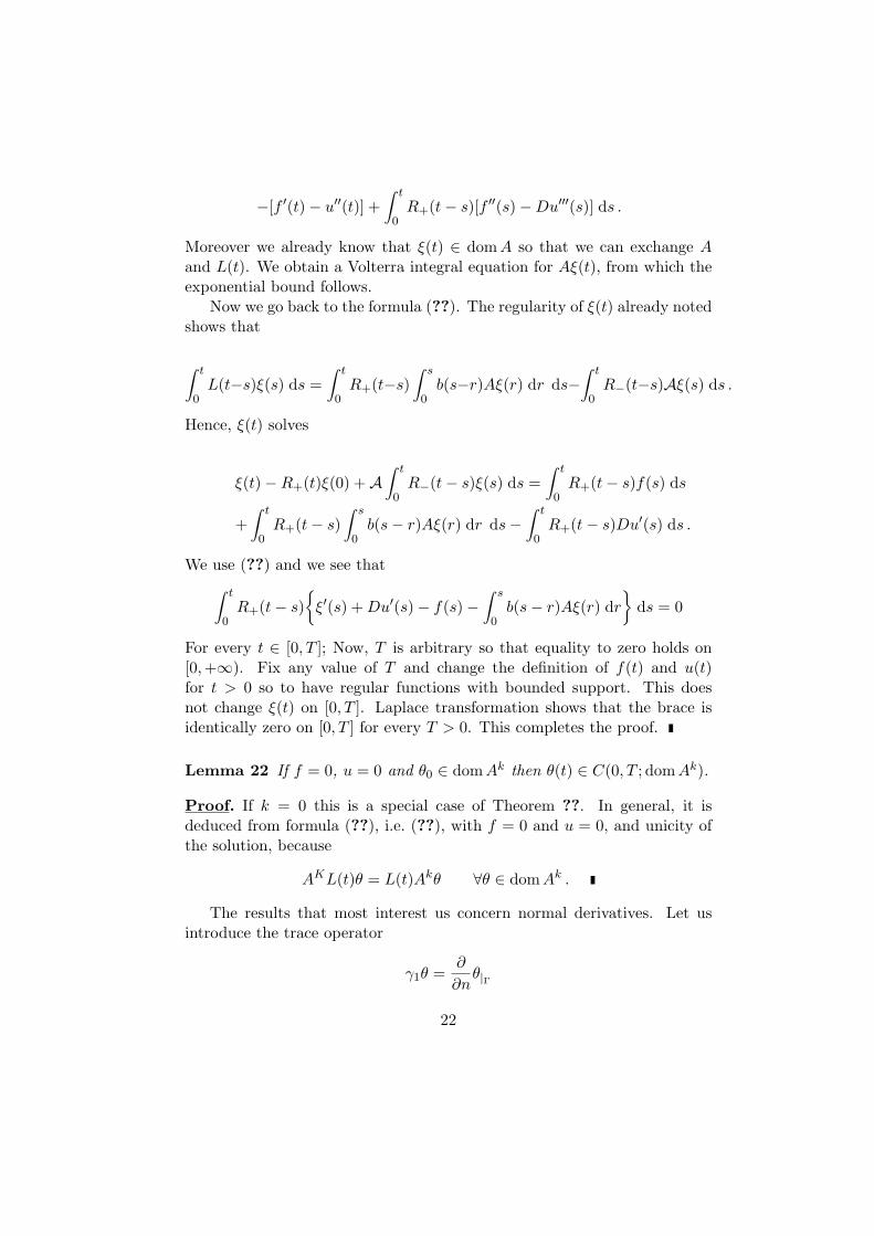
For every t ∈ [0, T ]; Now, T is arbitrary so that equality to zero holds on[0,+∞). Fix any value of T and change the definition of f(t) and u(t)for t > 0 so to have regular functions with bounded support. This doesnot change ξ(t) on [0, T ]. Laplace transformation shows that the brace isidentically zero on [0, T ] for every T > 0. This completes the proof.

Lemma 22 If f = 0, u = 0 and θ0 ∈ domAk then θ(t) ∈ C(0, T ; domAk).

Proof. If k = 0 this is a special case of Theorem ??. In general, it isdeduced from formula (??), i.e. (??), with f = 0 and u = 0, and unicity ofthe solution, because

AKL(t)θ = L(t)Akθ ∀θ ∈ domAk .

The results that most interest us concern normal derivatives. Let usintroduce the trace operator

γ1θ =∂

∂nθ|Γ

22

We now use the notation b ? θ to denote the convolution,

(b ? θ)(t) =∫ t

0b(t− s)θ(s) ds .

Lemma 23 Let u = 0, f = 0. We have:

γ1 (b ? θ) ∈ H−1(0, T ;L2(Γ))

and the transformation from θ0 ∈ L2(Ω) to γ1 (b ? θ) ∈ H−1(0, T ;L2(Γ)) iscontinuous.

Proof. The trace is well defined if θ0 is “regular”, i.e. θ0 ∈ domAk withk large. We prove continuity (in the stated sense) of the transformation,which is then extended by continuity to every θ0 ∈ L2(Ω).

It is known from [?] that

γ1θ = −D∗Aθ , θ ∈ domA .

For “regular” data and zero boundary condition and affine term we have

θ′(t; θ0) = b ? (Aθ(·; θ0)) = A(b ? θ(·; θ0)) .

Hence,

b ? θ(·; θ0) = A−1(θ′(t; θ0)) , γ1(b ? θ(·; θ0)) = D∗θ′(t; θ0) .

Let now θn be a sequence of “regular” initial data, θn → θ0 in L2(Ω). Weproved that the solutions converge in C(0, T ;L2(Ω)) so that

θ′(t; θn) → θ′(t; θ0) in H−1(0, T ;L2(Ω)) .

Hence, it is sufficient to prove that D∗ has a continuous extension as anoperator from H−1(0, T ;L2(Ω)) to H−1(0, T ;L2(Γ)). Let for this

D : (Du(·) )(t) = Du(t) .

Let φ ∈ H10 (0, T ;L2(Γ)), ψ ∈ H−1(0, T ;L2(Ω)). The operator D∗ is defined

by〈〈Dφ, ψ〉〉 = 〈〈φ, D∗ψ〉〉

(where 〈〈·, ·〉〉 denotes the proper pairing). This operator D∗ is the requiredextension by continuity of D∗ since, for ψ = ψ(t) a smooth function, equalityof the pairings is equivalent to∫ T

0〈Dφ(t, x), ψ(t, x)〉 dt =

∫ T

0〈Dφ(t, x), ψ(t, x)〉 dt

=∫ T

0〈φ(t, x), D∗ψ(t, x)〉 dt

23

where 〈·, ·〉 is the inner product in L2(Ω).

Let us consider now the wave equation

wtt = ∆w , w(0) = w0 , w′(0) = 0 in Ω , wΓ = 0 . (39)

It is known thatw(t) = R+(t)w0 , t ∈ IR

and if w0 ∈ H10 (Ω) then γ1w(t) exists as an element of L2(−T, T ;L2(Γ)).

Moreover,w0 −→ γ1w(t) = γ1[R+(t)w0] (40)

is continuous from w0 ∈ H10 (Ω) to L2(−T, T ;L2(Γ)) for every T > 0, see [?,

?, ?]. Here the full strength of the assumption made on Ω is needed.The sense in which the trace exists is as follows: it exists for the “regular”

vectors w0. It is proved the stated continuous dependence, so that the traceoperator is extended by continuity to every initial condition in H1

0 (Ω).We prove an analogous property of θ(t) but, instead then proving it

directly, with a computation that mimics, for example, that in [?], we deduceit from the property of the solution of the wave equation just recalled.

Theorem 24 Let f and u be zero. The transformation

θ0 → γ1θ

is continuous from H10 (Ω) to L2(0, T ;L2(Γ)) for every T > 0.

Proof. We proved (Lemma (??)) that if θ0 ∈ domAk then θ(t) ∈ domAk

for every t so that the trace γ1θ(t) exists in the usual sense, provided thatk is large enough. We prove continuity from H1

0 (Ω) to L2(G) so that thetransformation θ0 → γ1θ(t) can be extended to every initial condition θ0 ∈H1

0 (Ω).Let w(t) = R+(t)θ0 be the solution of problem (??) (with now w0 = θ0).

Then, θ(t) is the solution of the Volterra integral equation

θ(t) = w(t) +∫ t

0

[R+(t− s)b′(0)θ(s) +

∫ t−s

0R+(t− s− ν)b′′(ν)[θ(s)] dν

]ds

−∫ t

0b′(t− s)θ(s) ds . (41)

Let T > 0 be fixed. The properties of the wave equation recalled aboveshow that for every fixed s, the function

t −→ γ1 [R+(t− s)θ(s)]

24

is square integrable, hence it is integrable. We now proceed in two steps.Step 1) we prove that s→ γ1 [R+(t− s)θ(s)] exists and belongs to L2(G)

for a.e. t.We shall prove below that the function of s

s→∫ T

0γ1 [R+(t− s)θ(s)] dt (42)

is continuous, hence square integrable. Granted this we can integrate,∫ T

0

∣∣∣∣∣∣∣∣∫ T

0γ1 [R+(t− s)θ(s)] dt

∣∣∣∣∣∣∣∣2 ds

≤∫ T

0

T ·∫ T

0

∣∣∣∣∣∣∣∣γ1 [R+(t− s)θ(s)]∣∣∣∣∣∣∣∣2 dt

ds < +∞ . (43)

Now, Fubini theorem shows that the function

s −→ γ1 [R+(t− s)θ(s)]

exists a.e. and belongs to L2(G). Moreover,∫ T

0

∫ T

0||γ1R+(t− s)θ(s)||2 dt ds =

∫ T

0

∫ T−s

−s||γ1R+(r)θ(s)||2 dr ds

≤M ||θ||2L2(0,T ;H10 (Ω)) ≤ M ||θ0||2H1

0 (Ω) . (44)

Inequalities (??) and (??) show that the function

t −→∫ t

0γ1[R+(t− s)θ(s)] ds ,

as an element of L2(Q), depends continuously on θ0 ∈ H10 (Ω).

In order to complete this argument we prove continuity of the functionin (??). We represent∫ T

0

[γ1R+(t− s)θ(s)− γ1R+(t− s′)θ(s′)

]dt

=∫ T

0

[γ1R+(t− s)θ(s)− γ1R+(t− s)θ(s′)

]dt (45)

+∫ T

0

[γ1R+(t− s)θ(s′)− γ1R+(t− s′)θ(s′)

]dt (46)

We know from Theorem ?? point 1) that if θ0 ∈ H10 (Ω) = domA then the

solution θ(s) is continuous from s to H10 (Ω). Hence,

lims′→s

||θ(s)− θ(s′)||H10 (Ω) = 0 .

25

This shows that the integral in (??) tends to zero, thanks to the regularityof the trace operator of the wave equation.

The integral in (??) is represented as∫ T

0

[γ1R+(t− s′ + (s′ − s))θ(s′)− γ1R+(t− s′)θ(s′)

]dt .

This tends to zero for s − s′ → 0, thanks to the Lebesgue theorem on thecontinuity of the shift.

We recapitulate: we have now proved that γ1R+(t−s)θ(s) is well defined,as an element of L2, both as a function of t and as a function of s. In orderto complete the proof:

Step 2) we prove that the trace γ1θ(s) exists in L2(G) and dependscontinuously on θ0 ∈ H1

0 (Ω). We go back to the equation (??) that we nowrepresent as

θ(t) = F (t) +∫ t

0b′(t− s)θ(s) ds .

Here

F (t) = y(t)+∫ t

0

[R+(t− s)b′(0)θ(s) +

∫ t−s

0R+(t− s− ν)b′′(ν)[θ(s)] dν

]ds

and we proved that γ1F (t) ∈ L2(G) is a continuous function of θ0 ∈ H10 (Ω).

The function b′(t) is scalar, so that for θ0 ∈ domAk, k large enough, wehave

γ1θ(t) = γ1F (t) +∫ t

0k(t− s)γ1F (s) ds

where k(t) is the resolvent kernel of b′(t). The required continuity property ofγ1θ(t) now follows because the right hand side of this equality is a continuousfunction of γ1F (t) ∈ L2(G).

References

[1] Azamatov J, Lorenzi A (2002) Direct and inverse problems for evolutionintegro-differential equations of the first order in time. Univ. di Milano,Dip. di Matematica “F. Enriques”, quaderno n.16/2002.

[2] Barbu V. (1976) Nonlinear semigroups and differential equations inBanach spaces, Noordhoff, Leyden.

[3] Barbu V, Iannelli M (2000) Controllability of the heat equation withmemory. Diff Integral Eq 13:1393–1412.

26

[4] Belleni-Morante A (1978) An integro-differential equation arising fromthe theory of heat conduction in rigid materials with memory. BollUnione Mat Ital (5) 15-B:470–482.

[5] Benabdallah B, Naso MG (2000) Null controllability of a thermoelasticplate. Abstr Appl Anal 7:585–599.

[6] Da Prato G, Iannelli M (1980) Linear integro-differntial equations inBanach spaces. Rend Sem Mat Univ Padova 62:207–219.

[7] Da Prato G, Iannelli M, Sinestrari E (1983) Temporal regularity for aclass of integrodifferential equations in Banach spaces. Boll Unione MatItal (VI) 2-C:171–185.

[8] Davis PL (1975) Hyperbolic integrodifferential equations. Proc AmMath Soc 47:155-160.

[9] Davis PL (1976) On the hyperbolicity of the equations of the lineartheory of heat conduction for materials with memory. SIAM J ApplMath 30:75–80.

[10] Di Blasio G (1994) Parabolic Volterra integrodifferential equations ofconvolution type. J Integral Eq Appl 6:479–508.

[11] Favini A, Lorenzi A (2003) Singular integro-differential equations ofparabolic type and inverse problems. Math Models Meth in Appl Sci12:1745–1766.

[12] Fattorini HO (1985) Second order linear differential equations in Ba-nach spaces, North-Holland, Notas de Matematica (99), Amsterdam.

[13] Fridman A, Shimbrot M (1967) Volterra integral equations in Banachspaces. Trans Amer Math Soc 126:131-179.

[14] Grimmer RC, Miller RK (1977) Existence, uniqueness, and continuityfor integral equations in Banach spaces. J Math Anal Appl 57:429–447.

[15] Gurtin ME, Pipkin AG (1968) A general theory of heat conduction withfinite wave speed. Arch Rat Mech Anal 31:113–126.

[16] Kim JU (1992) Control of a plate equation with large memory. Diff IntEq 5:261–279.

[17] Komornik V (1994) Exact controllability and stabilization: the multi-plier method, Masson, Paris.

27

[18] Lasiecka I, Triggiani R (1981) A cosine operator approach toL2(0, T ;L2(Γ))–boundary input hyperbolic equations, Appl Mat Op-tim 7:35–93.

[19] Lasiecka I, Triggiani R (1983) Regularity of hyperbolic equations underL2(0, T ;L2(Γ))-Dirichlet boundary terms. Appl Mat Optim 10:275–286.

[20] Lasiecka I, Triggiani R (1988) Exact boundary controllability onL2(Ω)×H−1(Ω) of the wave equation with Dirichlet boundary controlacting on a portion of the boundary ∂Ω and related problems. ApplMat Optim 18:241–277.

[21] Lasiecka I, Triggiani R (2000) Control theory for partial differen-tial equations: continuous and approximation theories. II Abstracthyperbolic-like systems over a finite time horizon, Cambridge U.P.,Cambridge.

[22] Leugering G (1987) Time optimal boundary controllability of a simplelinear viscoelastic liquid. Math Meth Appl Sci 9:413–430.

[23] Lions JL (1988) Controlabilite exacte, perturbations et stabilization desystemes distribues, Vol. 1, Masson, Paris.

[24] Londen S-O (1978) An existence result on a Volterra equation in aBanach space. Trans Amer Math Soc 235:285–304.

[25] Miller RK (1975) Volterra integral equations in Banach spaces. FunkEkv 18:163-194.

[26] Munoz Rivera JE, Naso MG (2003) Exact boundary controllability inthermoelasticity with memory. Adv Diff Eq. 8:471–490.

[27] Pazy A (1983) Semigroups of linear operators and applications to par-tial differential equations, Springer-Verlag, New-York.

[28] Renardy M (1982) Some remarks on the propagation and non-propagation of discontinuities in linear viscoelastic liquids. RheologicaActa 21:251–254.

[29] Sova M (1966) Cosine operator functions. Rozprawy Mat 49:1–47.

[30] Yan J (1992) Controlabilite exacte pour des systemes a memoire. RevMat Univ Compl Madrid 5:319–327.

28

[31] Yong J, Zhang X, Exact controllability of the heat equation with hy-perbolic memory kernel, in Control of Partial Differential Equations,Lecture Notes in Pure and Applied Mathematics, Marcel Dekker, toappear.

29