Embed Size (px)
Citation preview
Control and Operation of a Vertical Axis Wind Turbine
Tiago André dos Santos Marques
Thesis to obtain the Master of Science Degree in
Mechanical Engineering
Supervisor: Prof. Luís Manuel de Carvalho Gato
Co-supervisor: Prof. Jörgen Svensson
Examination Committee
Chairperson: Prof. Viriato Sérgio de Almeida Semião
Supervisor: Prof. Luís Manuel de Carvalho Gato
Members of the Committee: Dra. Ana Isabel Lopes Estanqueiro
November 2014


I
Acknowledgments
First and foremost, I would like to express my appreciation to Professor Jörgen Svensson for the
opportunity to be involved in this project in a field that I have lately become more interested to work in
and for his valuable guidance and orientation throughout my work.
I would like to thank Lars Lindgren for the frequent knowledge input on various subjects and also
for the assistance in establishing the wind speed measurement connections on the roof.
I wish to acknowledge the support provided by Måns Andersson and Aleksandar Stojkovic in
understanding the previous programming of the microcontrollers.
Yury Loyaza pulled me out of several holes when my skills in LabVIEW were not enough to
reach my goals, I would like to thank him for that.
I would also like to show my appreciation to Evripidis Karatsivos for his patience to expand my
knowledge about synchronous machines in an initial phase of the project and to Getachew Darge, the
man of all trades who is always available to help, my gratitude for his time and dedication to design
and assemble the mechanical brake system.
To my friends I owe my sincere gratitude for the company and the good times and for the
encouragement to always do my best. Finally, I dedicate this work to my family for their unconditional
support and motivation and for the education that gave me the values that I will keep throughout my
life.

II
Abstract
Research in wind power generation technology is a topic of high relevance in the context of
renewable energy systems. This project aims to develop and implement an automatic operation and
control system for an experimental vertical axis wind turbine (VAWT) located at Lunds Tekniska
Högskola, in Lund, Sweden.
Supervisory control and data acquisition systems (SCADA) are increasingly considered
indispensable in industrial scale wind power plants with the purpose of optimizing power production
and monitoring the operation conditions in real-time to improve safety and reduce downtime and costs.
Variable speed control is widely used for maximizing power extraction. In this project, a
Maximum Power Point Tracking (MPPT) algorithm was successfully implemented in order to optimize
power production. Hill Climb Search (HCS) was the chosen control method, since there is no
knowledge about the optimum tip speed ratio of the rotor or the wind turbine maximum power curve.
A state-machine model was developed to manage the operation of the wind turbine. The control
sequence is implemented in programmable logic controllers from National Instruments, and data from
the power converters and wind speed measurement is acquired and analyzed in the system.
Performance tests were ran to investigate the optimum CP and the wind speed at which the wind
turbine is capable of producing power.
Keywords: Wind turbine control, Supervisory Control and Data Acquisition, PLC programming,
LabVIEW, Maximum Power Point Tracking, Hill-Climb search.

III
Resumo
A investigação em tecnologias de extracção de energia eólica tem sofrido rápida expansão no
âmbito das energias renováveis. O presente trabalho tem como objectivo desenvolver e implementar
um sistema de controlo e monitorização para uma turbina eólica de eixo vertical experimental,
instalada na Lunds Tekniska Högskola, em Lund, Suécia.
Sistemas de monitorização e aquisição de dados (SCADA) são cada vez mais indispensáveis
na industria de energia eólica, uma vez que o conhecimento preciso das condições de operação e
monitorização permanente dos parques eólicos permite optimizar a produção de energia, melhorar a
segurança das turbinas e reduzir períodos de inactividade.
Controlo de velocidade variável (Variable speed control) é amplamente utilizado para maximizar
a extracção de energia. Neste projecto, um algoritmo de Maximum Power Point Tracking foi
implementado com sucesso de modo a optimizar a produção. Hill Climb Search foi o método de
controlo escolhido, uma vez que não existe informação disponível acerca do tip speed ratio óptimo do
rotor ou da curva de potência da turbina.
Um state machine model foi desenvolvido com o objectivo de gerir os estados de operação da
turbina eólica e foi implementado em controladores lógicos programáveis da National Instruments. A
comunicação com os conversores de potência e medição da velocidade do vento foi estabelecida e
os dados são adquiridos e analisados pelo sistema em tempo real.
O sistema foi sujeito a testes para investigar a performance e averiguar o CP óptimo da turbina e
a velocidade do vento mínima para que ocorra produção de energia.
Palavras-chave: Controlo de turbinas eólicas, SCADA, programação de PLC, LabVIEW, Maximum
Power Point Tracking, Hill-Climb search.

IV
Table of Contents 1 Introduction ..................................................................................................................................... 1
1.1 Background.............................................................................................................................. 1
1.2 Objectives ................................................................................................................................ 3
1.3 Report outline .......................................................................................................................... 4
2 Wind Power overview ..................................................................................................................... 5
2.1 Technology .............................................................................................................................. 5
2.2 Wind characteristics and siting ................................................................................................ 8
2.3 Aerodynamics and power production ...................................................................................... 9
2.4 SCADA (Supervisory Control and Data Acquisition) ............................................................. 12
3 Wind turbine control theory ........................................................................................................... 14
3.1 Control and operation ............................................................................................................ 14
3.2 Control levels ......................................................................................................................... 15
3.2.1 Wind power system block structure ............................................................................... 16
3.3 Variable speed control ........................................................................................................... 17
3.3.1 Synchronous machines ................................................................................................. 18
3.4 Maximum power extraction strategy ...................................................................................... 18
3.4.1 Maximum Power Point Tracking methods ..................................................................... 18
4 LTH Wind Turbine unit .................................................................................................................. 22
4.1 Intended functions ................................................................................................................. 22
4.2 Control structure .................................................................................................................... 23
4.3 Measurements and communication ...................................................................................... 25
4.3.1 Wind turbine ................................................................................................................... 25
4.3.2 Meteorological mast ...................................................................................................... 25
4.3.3 Safety signals ................................................................................................................ 26
4.4 Technical specifications ......................................................................................................... 26
4.4.1 Wind turbine ................................................................................................................... 26
4.4.2 Transmission ................................................................................................................. 28
4.4.3 Mechanical brake........................................................................................................... 28
4.4.4 Meteorological mast ...................................................................................................... 29
4.4.5 Power converters ........................................................................................................... 30
4.5 Automation equipment and engineering tools ....................................................................... 32
4.5.1 Programming in LabVIEW ............................................................................................. 32
4.5.2 NI CompactRIO ............................................................................................................. 33
4.5.3 NI Compact RIOs in the control system: ....................................................................... 34
4.5.4 CompactRIO VS myRIO ................................................................................................ 34
5 Control implementation ................................................................................................................. 35
5.1 Control requirements ............................................................................................................. 35

V
5.2 System architecture ............................................................................................................... 35
5.3 Modes of operation ................................................................................................................ 36
5.3.1 Constant rotor speed ..................................................................................................... 36
5.3.2 Maximum power point tracking with induced start-up ................................................... 37
5.3.3 Maximum power point tracking with freewheeling start-up ........................................... 38
5.4 Plant system block structure .................................................................................................. 38
5.5 LabVIEW implementation ...................................................................................................... 42
5.5.1 Human Machine Interface ............................................................................................. 43
5.5.2 I/O Field Programmable Gate Array .............................................................................. 47
5.5.3 Wind speed sensor decoding ........................................................................................ 49
5.5.4 State machine implementation ...................................................................................... 51
5.5.5 Data logging ................................................................................................................... 62
5.5.6 Remote panel interface to Vattenhallen ........................................................................ 63
6 Performance tests on the wind turbine ......................................................................................... 64
6.1 Communication between the PLCs ....................................................................................... 64
6.2 State machine sequence ....................................................................................................... 65
6.3 Control modes ....................................................................................................................... 67
6.3.1 Constant rotor speed ..................................................................................................... 67
6.3.2 Maximum power extraction with induced start-up ......................................................... 71
6.3.3 Maximum power extraction with freewheeling start-up ................................................. 73
7 Discussion ..................................................................................................................................... 74
7.1 Performance tests ................................................................................................................. 74
7.2 Experimental conditions and sources of error ....................................................................... 75
7.3 Safety of the installation ........................................................................................................ 76
7.4 Evaluation of the success of the project ................................................................................ 77
8 Conclusions and recommendations for future work ..................................................................... 78
9 References .................................................................................................................................... 79
10 Appendices ................................................................................................................................... 81
10.1 Human Machine Interface ..................................................................................................... 81
10.2 LabVIEW screenshots ........................................................................................................... 81
List of Figures Figure 1 - Global cumulative wind power capacity 1995-2012 (IEA, Technology Roadmap Wind
Energy, 2013) .......................................................................................................................................... 2
Figure 2 - Left: Large-scale HAWT Siemens SWT-6.0MW-154m [www.siemens.com]; Right: Small-
scale VAWT in Environment Energy Centre, Leyland, UK [www.quietrevolution.com] .......................... 5
Figure 3 - Lift and drag type horizontal axis wind turbines (Eldrige, 1980) ............................................. 6

VI
Figure 4 - Lift type vertical axis wind turbines (Eldrige, 1980) ................................................................. 6
Figure 5 - Main components of a Darrieus vertical axis wind turbine system [www.kids.esdb.bg] ......... 7
Figure 6- Sample wind data (Manwell, 2009) .......................................................................................... 8
Figure 7 - Left: Experimental speed profile (Tempel, 2006); Right: Schematic of a momentum wake
over a building (Rohatgi & Nelson, 1994) ................................................................................................ 8
Figure 8 - Schematic of wind distribution over a building for the installation of a small-scale VAWT
[www.quietrevolution.com]....................................................................................................................... 9
Figure 9 - Power output as a function of rotor speed and optimal rotor speed points
[www.intechopen.com] .......................................................................................................................... 10
Figure 10- Power coefficient Cp plotted against tip speed ratio for various types of wind turbines (Örs,
2009) ...................................................................................................................................................... 10
Figure 11 - Typical wind turbine power curve (Manwell, 2009) ............................................................. 11
Figure 12 - Example of SCADA system control architecture [www.setec-windpower.com] ................. 13
Figure 13 - List of protection functions from "Guideline for the Certification of Wind Turbines“,
Germanischer Lloyd (GL Renewables Certification), Edition 2010 [www.dnvgl.com]........................... 14
Figure 14 - Control sub-systems (Manwell, 2009) ................................................................................ 15
Figure 15 - Wind power system block overview (Svensson, 2006)....................................................... 16
Figure 16 - HCS method. (a) Principle of the HCS method. (b) Control block diagram of the HCS
method (Barakati, Kazerani, & Aplevich, 2009) .................................................................................... 19
Figure 17 - Flow chart of the HCS control method (ΔP: variation in power; Δω: variation in rotor speed;
i*step: current reference step between iterations) ................................................................................... 20
Figure 18 - Wind turbine setup and control structure ............................................................................ 22
Figure 19 - Modular layout of the cabinets anticipating future expansion of the production site .......... 24
Figure 20 - Cabinets with the power converters and microcontrollers .................................................. 25
Figure 21 - Wind turbine installation on the rooftop .............................................................................. 27
Figure 22 - Schematic and picture of the siting of the wind turbine ...................................................... 27
Figure 23 - Transmission belt, WT shaft, drum brake and PMSG ........................................................ 28
Figure 24 - Mechanical brake components ........................................................................................... 28
Figure 25 - Meteorological mast ............................................................................................................ 29
Figure 26 - Live webcam streaming of the wind turbine rotor ............................................................... 30
Figure 27 - Voltage measurement equipment ....................................................................................... 31
Figure 28 - Cabinets with the electrical converters ............................................................................... 31
Figure 29 - NI Compact RIO 9022 [www.ni.com/compactrio] ............................................................... 33
Figure 30 - Wind turbine setup and control structure ............................................................................ 35
Figure 31 - Power output VS wind speed for a constant rotor speed [www.intechopen.com] .............. 36
Figure 32 - Optimum Power Production mode ...................................................................................... 37
Figure 33 - Wind Turbine control sequence .......................................................................................... 39
Figure 34- Current PID controllers ........................................................................................................ 43
Figure 35 - Generator speed PI controller ............................................................................................. 43
Figure 36- Human Machine Interface with Main tab ............................................................................. 44
VII
Figure 37 - HMI Converters tab ............................................................................................................. 45
Figure 38 - HMI Constant speed tab ..................................................................................................... 46
Figure 39 - HMI MPPT tab..................................................................................................................... 46
Figure 40 - Read from FPGA ................................................................................................................ 47
Figure 41 - Write to the generator side FPGA ....................................................................................... 48
Figure 42 - Notification lights on the grid side cabinet .......................................................................... 49
Figure 43 - Anemometer voltage decoding in the FPGA ...................................................................... 49
Figure 44 - Wind speed calculation in the real-time controller .............................................................. 50
Figure 45 - Initialization of variables ...................................................................................................... 51
Figure 46 - State machine OFF state .................................................................................................... 52
Figure 47 - State machine ACTIVATE state .......................................................................................... 53
Figure 48 - Start/stop regulating signals to the generator and grid side FPGAs ................................... 53
Figure 49 - State machine READY state ............................................................................................... 54
Figure 50 - Start-up control mode confirmation ..................................................................................... 54
Figure 51 - State machine START UP state (Freewheel start-up) ........................................................ 55
Figure 52 - State machine START UP state (Motor start-up) ............................................................... 55
Figure 53 - While loop to start the generator as a motor ....................................................................... 56
Figure 54 - While loop to run the generator at constant speed (continuation of Figure 54) .................. 57
Figure 55 - MPPT Motor state (Part 1) .................................................................................................. 58
Figure 56 - MPPT Motor state (Part 2 True) .......................................................................................... 59
Figure 57 - MPPT Motor state (Part2 False) ......................................................................................... 59
Figure 58 - MPPT Motor state (Part 3) .................................................................................................. 60
Figure 59 - State machine SHUTDOWN state ...................................................................................... 60
Figure 60 - State machine MPPT state ................................................................................................. 61
Figure 61 - State machine DEACTIVATE state..................................................................................... 61
Figure 62 - Data logger while loop ........................................................................................................ 62
Figure 63 - Write to measurement file VI ............................................................................................... 63
Figure 64 - Remote panel interface for Vattenhallen ............................................................................ 63
Figure 65 - Communication tests on the PLCs...................................................................................... 64
Figure 66 - Code of the communication test in the GRID side FPGA VI to apply the increment .......... 64
Figure 67 - Code of the communication test on the GRID side real time module ................................. 65
Figure 68 - Communication test with the NET side RT (Left) and with the GRID side RT (Right) ........ 65
Figure 69 - Control sequence states in execution ................................................................................. 65
Figure 70 - Control sequence experimental VI ...................................................................................... 66
Figure 71 - Wind speed measurement before correction ...................................................................... 66
Figure 72 - Wind speed measurement after correction with a 15μF capacitor ..................................... 67
Figure 73 - Constant mode performance test ........................................................................................ 67
Figure 74 - Test at different rotor speeds up until 150 rpm ................................................................... 69
Figure 75 - Power fluctuations due to the effect of the wind at 150 rpm ............................................... 69
Figure 76 - Polynomial regression of the power and wind speed ......................................................... 70

VIII
Figure 77 - Plot of power VS tip speed ratio dispersion ........................................................................ 71
Figure 78 - Performance test of the MPPT Motor method .................................................................... 72
Figure 79 - Close-up of the MPPT Motor test ........................................................................................ 73
Figure 80 - Oscillations in rotor speed measurement with fake theta off .............................................. 74
Figure 81 - Illustration of the dispersion of operating points due to unsteady wind speeds ................. 75
Figure 82 - Average wind speed in Malmö, Sweden [www.weather-and-climate.com] ........................ 75
Figure 83 - CFD simulation of the wind speed distribution around a building ....................................... 76
Figure 84 - HMI Datalogger tab ............................................................................................................. 81
Figure 85 - HMI Vattenhallen LTH tab ................................................................................................... 82
Figure 86 - HMI Weather data tab ......................................................................................................... 82
Figure 87 - HMI Errors tab ..................................................................................................................... 83
Figure 88 - HMI Sensors tab ................................................................................................................. 83
List of Tables
Table 1- Wind turbine technical specifications .......................................................................................26
Table 2 - Measurement Equipment ........................................................................................................30
Table 3 - State sequence transition conditions ......................................................................................40
Table 4 - Safety signals from the FPGA .................................................................................................47
Table 5- Control sequence main states variable States .........................................................................51
Table 6 - Rotor speed control mode .......................................................................................................56
Table 7- Variables saved by the data logger ..........................................................................................62
Table 8 - Polynomial regression results .................................................................................................70
Table 9 - Tip speed ratios correspondent to minimum power consumption ..........................................71

IX
Nomenclature
Symbols
ρ - Air density [kg/m3]
A - Rotor swept area [m2]
U - Wind speed [m/s]
CP - Power coefficient
β - Pitch angle
λ - Tip-speed ratio
Ω - Wind turbine rotor angular speed [rad/s]
R - Wind turbine rotor radius [m]
ωopt - Optimum rotor speed [rad/s]
λopt - Optimum tip-speed ratio
ΩWT - VAWT rotor speed [rpm]
fGEN - Generator frequency [Hz]
T - Torque [Nm]
- Average wind speed [m/s]
Abbreviations
PMSG - Permanent magnet synchronous generator
GRID SIDE - Electrical grid power converter
GEN SIDE - PMSG power converter
MPPT - Maximum Power Point Tracking

1
1 Introduction
1.1 Background
There is a growing awareness of the urgent need to find an alternative to the finite fossil
resources on which our energetic and industrial systems are based. The continuous growth of energy
demand of the last decades, aggravated by the exponential increase in consumption from emerging
economies (IEA, Key World Energy Statistics, 2013), has compelled governments and institutions to
intervene by stimulating technological advances in the renewable energy field, due to environmental
considerations in an effort to slow down climate change.
The success of the implementation of renewable energy systems has been driven by policy
support that has grown considerably during the last decade. Either focused on utility-scale or small-
scale generation systems, policies continue to evolve in order to address market developments and
reduce costs to promote massive installation. The EU 2020 Climate and Energy Package is an
example of policy making in Europe, consisting of a set of binding legislation which aims to ensure that
the European Union meets its targets for 2020: achieving 20% reduction in greenhouse gas emissions
from 1990 levels; raising the share of renewable energy consumption to 20% and making a 20%
improvement in EU's energy efficiency (EU, 2007).
The path for the creation of a global clean and sustainable energy platform is being walked one
step farther every day, as research in renewable energies is strongly encouraged and new
technologies emerge as a result. Wind power is considered to be one of the renewable energy
conversion technologies showing most developments in the recent years (IEA, Technology Roadmap
Wind Energy, 2013), as researchers and industries invest their knowledge in improving and optimizing
wind turbine systems for optimal energy yield and maximum performance. The author's intention is
that this project may contribute as a small step on that path.
Generating electrical power from the wind is an idea as old as electricity itself, but technological
developments have only made it viable as a large scale solution in the recent decades (Manwell,
2009). Wind has great potential for powering civilization, since it exists everywhere on earth and with a
considerable energy density in some places, which justifies the great investment and fast spreading of
this renewable energy conversion system.
Wind power industry has experienced tremendous growth over the last decade, with the global
installed capacity increasing from 18 GW in 2000 to approximately 300 GW in 2013, which represents
more than a 16 fold increase, as illustrated in Figure 1. Wind power now provides 2,5% of global
electricity demand, with some countries having considerable shares of their electricity production
coming from wind, with up to 30% in Denmark, 20% in Portugal and 18% in Spain (IEA, Technology
Roadmap Wind Energy, 2013).

2
Figure 1 - Global cumulative wind power capacity 1995-2012 (IEA, Technology Roadmap Wind
Energy, 2013)
Achieving the policy targets requires scaling up the current annual installed power capacity and
improving energy yields, while reducing downtime and operation and maintenance costs (O&M). The
installed capacity is increasing globally at a fast pace due to turbine technological maturity, policy
development and higher economical viability (IEA, Technology Roadmap Wind Energy, 2013).
Turbine technological improvements have been one of the main reasons for the significantly
increased capacity of the past decade, but even with such improvements turbines must be properly
maintained to achieve optimal production and meet revenue targets. Nowadays, monitoring is
indispensable to ensure that the turbines are operating at optimum conditions and maximum
performance (Sharpley, 2014).
Modern wind power plants rely on complex monitoring and control systems that allow controlling
individual turbines and displaying detailed information about their operating conditions. Supervisory
Control and Data Acquisition (SCADA) systems establish the communication between the plant
supervisor and the individual wind turbines, allowing starting and stopping power production and
gathering relevant information. This information typically includes wind speed and direction, turbine
operating states, individual power production, wind turbine rotor speed, pitch angle, internal sensor
signals, fault reports or maintenance requests. This data can be accessed remotely by an operator
and analysed in real-time, to assess the performance of the turbines by visualizing the power curve
and other parameters, enabling to maximize power production (Manwell, 2009).
A method for maximizing wind power extraction consists in implementing variable rotor speed
operation through the use of power converters. Static converters, used as an interface to the electric
grid, enable variable speed operation allowing for active control of the extracted power. Due to
external perturbations such as wind shear, tower shadows and random wind fluctuation, variable
speed control seems to be a good option for optimizing wind turbine operation (Zinger & Muljadi,

3
1997). The energy available in the wind varies continually as wind speed changes, and the amount of
power output from a wind energy conversion system is highly dependent upon the relation between
wind speed and rotor speed. By controlling rotor speed to achieve an optimal relation with wind speed,
improvements of over 10% in energy output have been documented, as well as lower mechanical
stress and less power fluctuation (Wang, 2004). In order to fully avail the advantages that outcome
from variable speed wind generation systems, it is necessary to develop advanced control methods to
extract maximum power output at different wind speeds. Research has been made on several different
strategies to achieve this, such as tip speed ratio control, power signal feedback control and hill-climb
search control (Thongam & Ouhrouche, 2011).
1.2 Objectives
In this context, the main purpose of this project is to fully develop and implement an automatic
monitoring and control system for the vertical axis wind turbine sited on top of the Mechanical
Engineering building in Lunds Tekniska Högskola (LTH), to perform overall control tasks and
monitoring to guarantee a safe and optimized operation. It is intended to:
Design an overall control system to enable automatic operation of the wind turbine setup and
implement it on the programmable logic controllers;
Implement an efficient control algorithm for maximum power extraction;
Install an automatic mechanical brake system on the wind turbine shaft to improve safety;
Update the functions of the web based remote panel interface to LTH science observation
centre, Vattenhallen;
Evaluate the performance and controllability of the wind turbine;
Investigate the efficiency of the system through performance tests.
The installation of the wind turbine in the university facilities is itself a visible manifestation of the
interest and commitment of the university in exploring and developing new technologies for renewable
energy generation, contributing for a cleaner environment and a more self-sustainable energetic
system. The wind turbine setup results from the cooperation between the manufacturing company
EXAMEC and LTH, and was erected in 2011 as part of a master's thesis project (Petitfils, 2011).
The wind turbine setup was designed in such a way to allow expansion to a multi-source station,
with the possibility to install new generation units. Modularity and adaptability are important features of
the system. This work is thus relatable to what is implemented in large scale installations such as
offshore wind power plants, since the monitoring of the experimental setup and the control philosophy
and structure are the same as in industrial scale applications. The programming tool used for the
implementation is NI LabVIEW and the program is operating in a commercial real-time embedded
reconfigurable controller from National Instruments, widely used throughout wind power industry
(Dvorak, Windpower Engineering & Development, 2014).

4
1.3 Report outline
This document is organized in eight chapters, from which the present section constitutes the
introduction and includes an overview of the background and relevance of the study of wind power
systems, as well as a description of the overall project objectives.
Chapter 2 provides an overview on wind power technology and addresses the different wind
turbine types available, the importance of studying wind characteristics for the siting of a wind power
generation unit, the aerodynamics of wind turbines and its role in power production and also an
overview on SCADA systems.
Chapter 3 presents the theory behind wind power plant control, including variable wind speed
control and the method to optimize power production in which this work was based.
In chapter 4 the wind turbine setup in which the control is performed is thoroughly described.
Chapter 5 presents the implementation, describing control architecture, the plant system block
structure, the operating modes and the programming in LabVIEW.
In chapter 6 the results from the performance tests ran on the system are presented.
Chapter 7 presents a discussion of the results and the main considerations about the
experimental conditions and the performance assessment, and an evaluation of the success of the
project. Recommendations for future experimental research on the setup are provided.
Chapter 8 encloses this document with the essential conclusions taken from the work performed.
5
2 Wind Power overview
It is useful to consider some fundamental facts underlying wind turbine operation before
proceeding. To understand how wind turbines function, this chapter provides a brief overview on the
available technology of modern wind turbines, wind resource characteristics and the physics behind
the aerodynamic interactions that ultimately result in power production.
2.1 Technology
A wind turbine is a machine that converts the kinetic energy present in the atmospheric air flow
into usable electricity. Wind turbines produce energy only in response to the immediately available
wind resource, thus the resultant power output is inherently fluctuating and non-dispatchable.
Wind turbines are connected to an electrical network, which can be residential or industrial scale
power systems, isolated or island networks, and large utility grids. In terms of generating capacity, the
turbines that make up the largest share of power production are generally rather large-scale turbines -
2 to 5 MW rated power (Manwell, 2009). However, small scale turbines (kilowatts scale) are becoming
gradually marketable, especially in remote places where grid based electricity is not available or
unreliable.
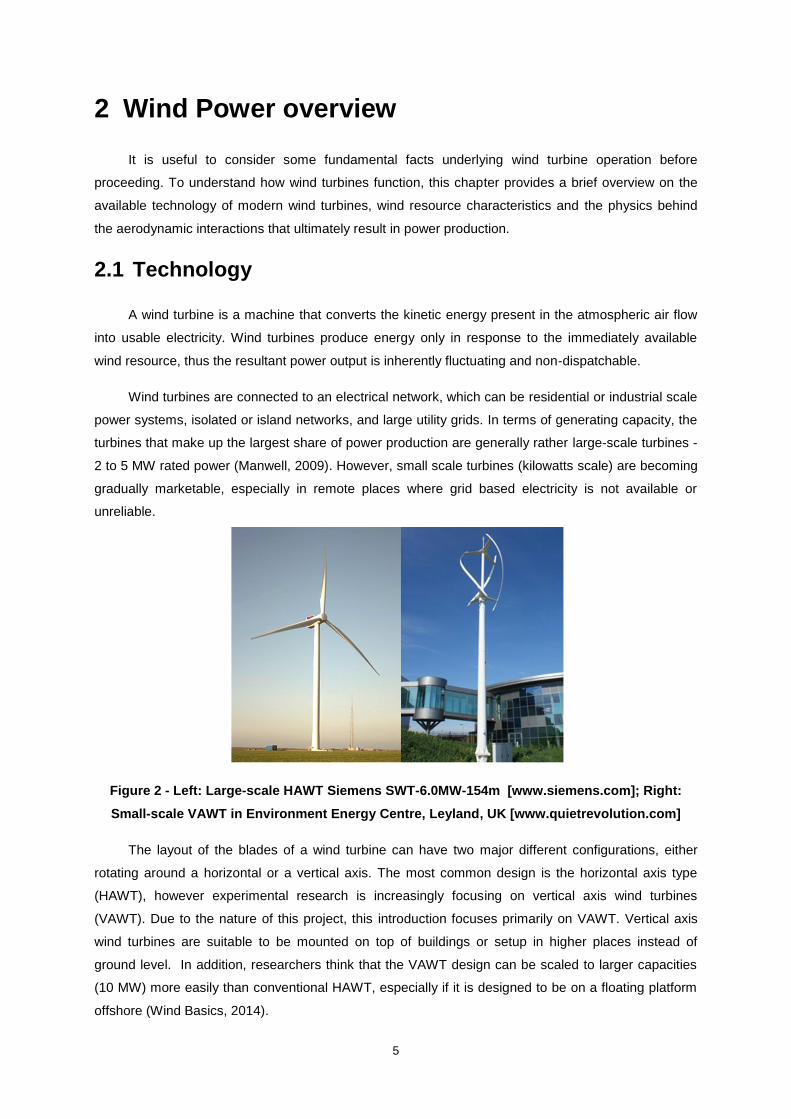
Figure 2 - Left: Large-scale HAWT Siemens SWT-6.0MW-154m [www.siemens.com]; Right:
Small-scale VAWT in Environment Energy Centre, Leyland, UK [www.quietrevolution.com]
The layout of the blades of a wind turbine can have two major different configurations, either
rotating around a horizontal or a vertical axis. The most common design is the horizontal axis type
(HAWT), however experimental research is increasingly focusing on vertical axis wind turbines
(VAWT). Due to the nature of this project, this introduction focuses primarily on VAWT. Vertical axis
wind turbines are suitable to be mounted on top of buildings or setup in higher places instead of
ground level. In addition, researchers think that the VAWT design can be scaled to larger capacities
(10 MW) more easily than conventional HAWT, especially if it is designed to be on a floating platform
offshore (Wind Basics, 2014).

6
A variety of different concepts for HAWT and VAWT have been proposed throughout the years,
as illustrated in Figure 3 and 4. Typically, commercially available wind turbines have two to three
blades, although many other designs have been tried.
Figure 3 - Lift and drag type horizontal axis wind turbines (Eldrige, 1980)
Figure 4 - Lift type vertical axis wind turbines (Eldrige, 1980)
In comparison to horizontal axis wind turbines, VAWTs have the following advantages:
Performance is independent from wind direction (omnidirectional), thus not requiring any special
mechanisms for yawing into wind;
Blades can be manufactured by mass production extrusion, since they are often untwisted and
of constant chord;
The generator is installed on the base, which makes maintenance simpler and cheaper.
However, up until now none of the types of VAWT could be developed to such a point that their
theoretical advantages would outweigh their practical disadvantages, in order to surpass the matured
technology of HAWT. Some important disadvantages of VAWTs are e.g. that the generator is located
on the base, which limits the height of the tower and thus the access to higher and steadier winds and
also the decrease in aerodynamic efficiency due to the existence of dead aerodynamic zones for the
blades on the opposite side to the incoming wind. A solution to overcome this limitation is to install the
VAWTs on top of buildings.
The principal subsystems of a typical wind turbine include (Manwell, 2009):
Rotor: The rotor consists of the hub and blades of the wind turbine. The blades are often
considered the most important components of a wind turbine since they are responsible for the
aerodynamic interaction with the wind, from which performance is largely dependent. The blades are
commonly manufactured from composites, primarily fibre glass or carbon fibre reinforced plastics.

7
Drive train: The drive train consists of the rotating parts that follow the rotor. This is typically
constituted by a low-speed shaft on the rotor side, a gearbox and a high-speed shaft on the generator
side. The purpose of the gearbox is to increase the rate of rotation of the rotor to a higher speed,
suitable for driving the electrical generator.
Generator: Induction or synchronous generators are the most commonly used in wind turbines.
The generator is of course the component responsible for transforming the mechanical power
harnessed from the wind into usable electricity.
Tower: The principal type of tower design currently in use is free-standing type using steel tubes
or lattice towers, although the latter is less common and usually for small-scale turbines. The stiffness
of the tower is an important factor since it is subject to cyclic loads and there is the possibility of
coupled vibrations between the rotor and the tower.
Controls: The control system of a wind turbine is a central subsystem, relevant both from the
machine operation and power production point of view. The control system is responsible for keeping
performance at optimum levels, by monitoring the operating conditions and respond accordingly in an
intelligent manner. The design of a control system for a wind turbine application follows traditional
control engineering practices. A wind turbine control system includes the following components:
o Sensors: measurement of important quantities such as rotor speed, yawing position, internal
temperature, current, voltage, etc.
o Controllers: mechanical mechanisms, electrical circuits;
o Power amplifiers: switches, electrical amplifiers, hydraulic pumps and valves;
o Actuators: motors, pistons, magnets and solenoids;
o Intelligence: computers, microprocessors, programmable embedded systems.
Figure 5 - Main components of a Darrieus vertical axis wind turbine system [www.kids.esdb.bg]
8
2.2 Wind characteristics and siting
The source of atmospheric air movement is the uneven heating of the Earth's surface by solar
radiation. Pressure differences across the globe cause air masses to displace and thus create the
phenomenon called wind.
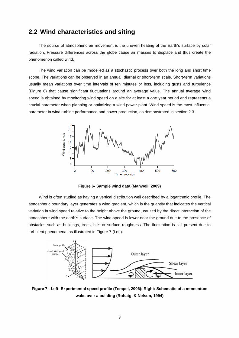
The wind variation can be modelled as a stochastic process over both the long and short time
scope. The variations can be observed in an annual, diurnal or short-term scale. Short-term variations
usually mean variations over time intervals of ten minutes or less, including gusts and turbulence
(Figure 6) that cause significant fluctuations around an average value. The annual average wind
speed is obtained by monitoring wind speed on a site for at least a one year period and represents a
crucial parameter when planning or optimizing a wind power plant. Wind speed is the most influential
parameter in wind turbine performance and power production, as demonstrated in section 2.3.
Figure 6- Sample wind data (Manwell, 2009)
Wind is often studied as having a vertical distribution well described by a logarithmic profile. The
atmospheric boundary layer generates a wind gradient, which is the quantity that indicates the vertical
variation in wind speed relative to the height above the ground, caused by the direct interaction of the
atmosphere with the earth's surface. The wind speed is lower near the ground due to the presence of
obstacles such as buildings, trees, hills or surface roughness. The fluctuation is still present due to
turbulent phenomena, as illustrated in Figure 7 (Left).
Figure 7 - Left: Experimental speed profile (Tempel, 2006); Right: Schematic of a momentum
wake over a building (Rohatgi & Nelson, 1994)
9
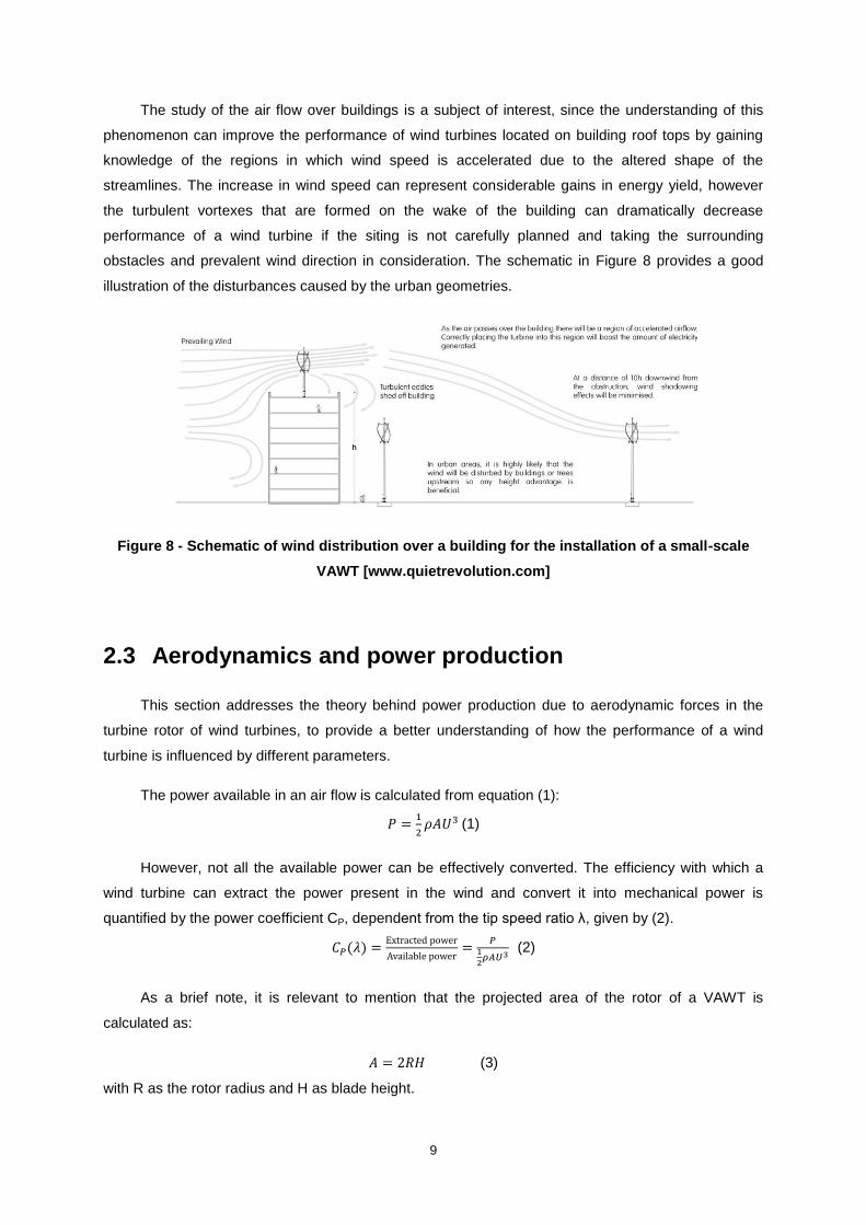
The study of the air flow over buildings is a subject of interest, since the understanding of this
phenomenon can improve the performance of wind turbines located on building roof tops by gaining
knowledge of the regions in which wind speed is accelerated due to the altered shape of the
streamlines. The increase in wind speed can represent considerable gains in energy yield, however
the turbulent vortexes that are formed on the wake of the building can dramatically decrease
performance of a wind turbine if the siting is not carefully planned and taking the surrounding
obstacles and prevalent wind direction in consideration. The schematic in Figure 8 provides a good
illustration of the disturbances caused by the urban geometries.
Figure 8 - Schematic of wind distribution over a building for the installation of a small-scale
VAWT [www.quietrevolution.com]
2.3 Aerodynamics and power production
This section addresses the theory behind power production due to aerodynamic forces in the
turbine rotor of wind turbines, to provide a better understanding of how the performance of a wind
turbine is influenced by different parameters.
The power available in an air flow is calculated from equation (1):
(1)
However, not all the available power can be effectively converted. The efficiency with which a
wind turbine can extract the power present in the wind and convert it into mechanical power is
quantified by the power coefficient CP, dependent from the tip speed ratio λ, given by (2).
(2)
As a brief note, it is relevant to mention that the projected area of the rotor of a VAWT is
calculated as:
(3)
with R as the rotor radius and H as blade height.
10
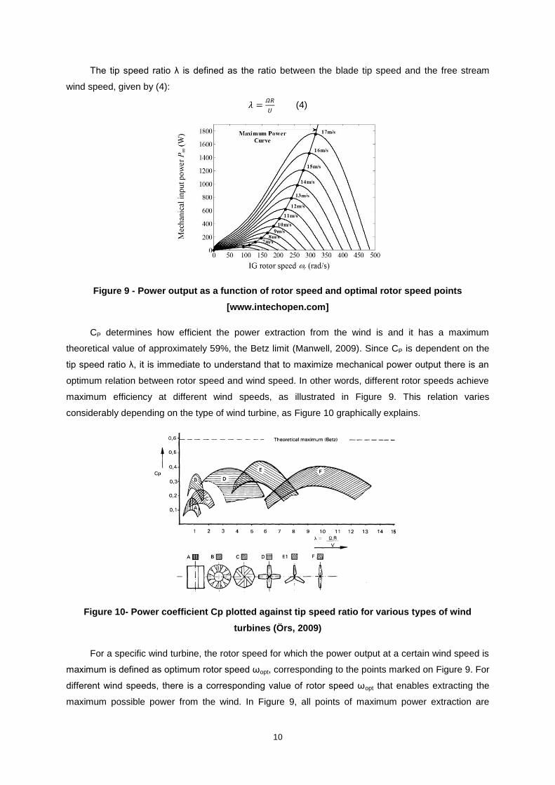
The tip speed ratio λ is defined as the ratio between the blade tip speed and the free stream
wind speed, given by (4):
(4)
Figure 9 - Power output as a function of rotor speed and optimal rotor speed points
[www.intechopen.com]
CP determines how efficient the power extraction from the wind is and it has a maximum
theoretical value of approximately 59%, the Betz limit (Manwell, 2009). Since CP is dependent on the
tip speed ratio λ, it is immediate to understand that to maximize mechanical power output there is an
optimum relation between rotor speed and wind speed. In other words, different rotor speeds achieve
maximum efficiency at different wind speeds, as illustrated in Figure 9. This relation varies
considerably depending on the type of wind turbine, as Figure 10 graphically explains.
Figure 10- Power coefficient Cp plotted against tip speed ratio for various types of wind
turbines (Örs, 2009)
For a specific wind turbine, the rotor speed for which the power output at a certain wind speed is
maximum is defined as optimum rotor speed ωopt, corresponding to the points marked on Figure 9. For
different wind speeds, there is a corresponding value of rotor speed ωopt that enables extracting the
maximum possible power from the wind. In Figure 9, all points of maximum power extraction are

11
connected by a line that represents the optimal tip speed ratio λopt. In order to maximize power
extraction, a wind turbine should always operate as close to λopt as possible. A way to achieve this is
by controlling the turbine rotor speed, to ensure that optimum rotor speed ωopt is maintained for every
wind speed value.
Figure 11 - Typical wind turbine power curve (Manwell, 2009)
The power curve of a wind turbine allows predicting the energy production without considering
all the inherent technical details of its various components (Manwell, 2009). With knowledge of the
power output and a measurement of wind speed, a characteristic power performance curve of the
wind turbine can be mapped, which usually can be obtained from the turbine manufacturer.
The relevant points of the curve are:
Cut-in wind speed: the minimum wind speed at which the machine will deliver power output,
although far from its optimum performance;
Rated wind speed: wind speed at which the turbine delivers its rated power;
Cut-out wind speed: the maximum wind speed at which the turbine is allowed to deliver power,
usually limited by structural and safety constraints.
The control strategy varies depending on if the turbine is operating below or above rated speed.
At low wind speeds the turbine control aims to maintain an optimum power coefficient Cp to extract as
much energy as possible, by operating at optimal rotational speed ωopt. Once the maximum allowable
rotor speed is reached, the mode of operation is changed in order to limit the power (rated power),
which involves reducing the rotor speed and the rotor efficiency using mechanical or electrical
mechanisms. This can be done with fixed rotor speed or variable rotor speed strategies.
There are different strategies to achieve the same goals. Pitch and stall regulation are two
common ways of controlling the power coefficient and power output, both for variable speed and fixed
speed wind turbines. Details about pitch control, stall control and power control are provided in chapter
3.3.
To gather information about the parameters that control the efficiency and power production of a
wind turbine, it is necessary to have systems that accurately monitor the operation and provide

12
relevant data to better understand the conditions and maximize the performance. The next section
provides an overview on the control systems that are implemented to satisfy this necessity.
2.4 SCADA (Supervisory Control and Data Acquisition)
SCADA (Supervisory Control and Data Acquisition) systems are significantly important control
systems used in large scale industrial infrastructures such as electric grids, water supplies and power
plants. Its function is to control and monitor industrial processes and to apply intelligent management
algorithms in order to make decisions over the system operation, taking into account the acquired data
and the status of the different components. An important function is to monitor alarm signals in the
system and apply safety measures or inform the control room of the detailed alarm conditions.
Data acquisition is performed by the measurement equipment and communicated to the overall
control system. The data is then compiled and formatted in such a way that the system can analyze it
and behave according to the control algorithm designed for the setup. It also provides the control
operator with the possibility to override the normal operating sequence through a Human Machine
Interface (HMI), if necessary.
Real-time monitoring and control systems are common in most electric power-generation
utilities. However, these systems were not used in early wind power plant facilities. As the number of
installed capacity increased and the share of power from wind integrated in power grids became
relevant, the industry recognized the value of optimizing production around the clock.
In case of a safety fault, the control system acts by removing the turbine from service as a
security measure. Routinely acquiring data from the wind turbines on an industrial wind power plant
via the SCADA system provides an additional opportunity to discover losses in production and ensure
that the wind power plant is operating at its maximum performance. The data, collected on a nearly
real-time basis, annually creates many terabytes of information about e.g. wind speed, generator
power output, rotor speed, pitch and yaw angles, etc (Dvorak, Windpower Engineering &
Development, 2014). Performance analysis can improve wind turbine operation in a significant way
and contribute to larger energy yields by allowing for immediate action when under-performance
problems arise.
The SCADA system consists of the bi-directional interaction between the acquired signals in the
wind turbine components, communicated to a data acquisition centre where the data is analyzed and
pre-programmed signals are sent back to the wind turbine as a response to the status and operating
conditions. The data is recorded and can be used for tracking errors and performance analysis.
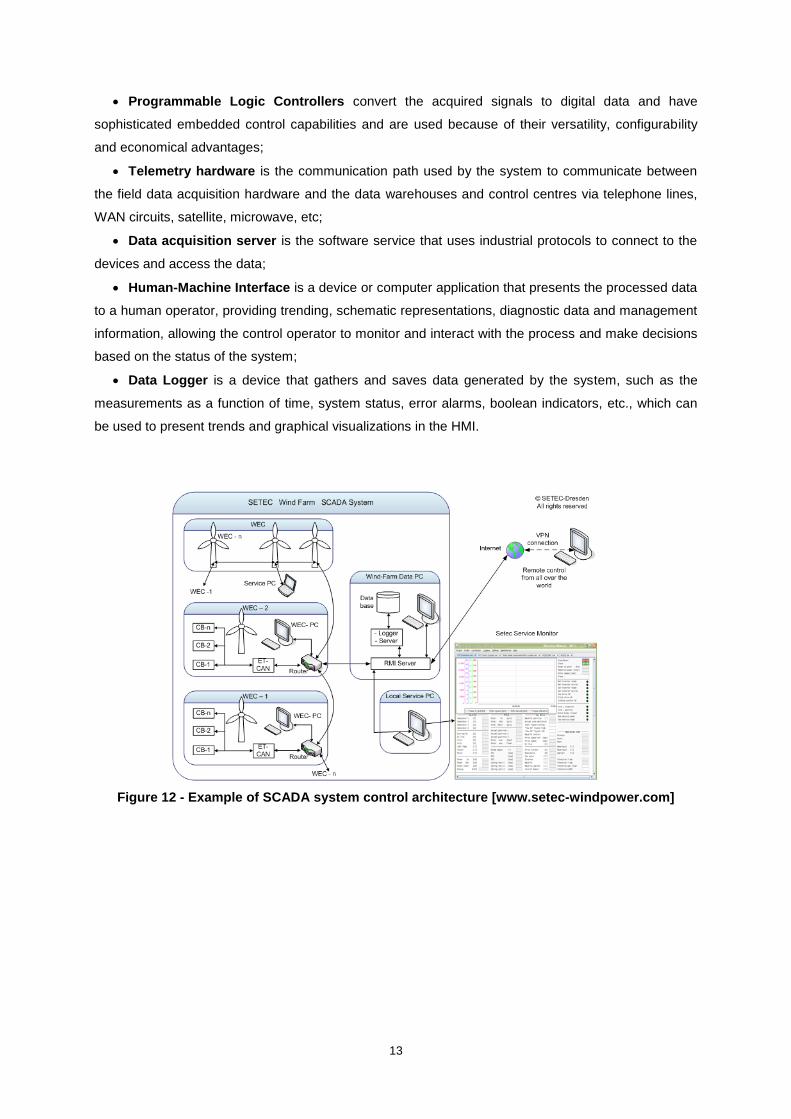
A brief description of the main subsystems of a SCADA system follows (Boyer, 2010) and an
illustration of an example of SCADA system architecture is provided in Figure 12:
13
Programmable Logic Controllers convert the acquired signals to digital data and have
sophisticated embedded control capabilities and are used because of their versatility, configurability
and economical advantages;
Telemetry hardware is the communication path used by the system to communicate between
the field data acquisition hardware and the data warehouses and control centres via telephone lines,
WAN circuits, satellite, microwave, etc;
Data acquisition server is the software service that uses industrial protocols to connect to the
devices and access the data;
Human-Machine Interface is a device or computer application that presents the processed data
to a human operator, providing trending, schematic representations, diagnostic data and management
information, allowing the control operator to monitor and interact with the process and make decisions
based on the status of the system;
Data Logger is a device that gathers and saves data generated by the system, such as the
measurements as a function of time, system status, error alarms, boolean indicators, etc., which can
be used to present trends and graphical visualizations in the HMI.
Figure 12 - Example of SCADA system control architecture [www.setec-windpower.com]

14
3 Wind turbine control theory
3.1 Control and operation
Without some form of control system, a modern wind turbine cannot successfully and safely
produce power. This section provides an insight on wind turbine control structure and the important
aspects of control systems that are relevant to wind turbine control. In general, the purpose of wind
turbine operation monitoring and control is to:
Ensure safety of the setup and the surroundings by continuously monitoring the internal
operation conditions, such as gearbox lubrication and temperature, as well as structural loads and
fatigue loads caused by the inherent aerodynamic load fluctuations;
Enable quick reaction in case of system failure or malfunction;
Define clear operation states for full power production (cut-in and cut-out wind speeds), start-up,
shutdown, and allow interaction with an operator for the eventuality of an emergency shutdown,
performing maintenance tasks, etc;
Maximize power production according to wind conditions using an optimum power extraction
control strategy;
Optimize economical return by minimizing maintenance interventions, increasing availability and
power production, and also by avoiding hazardous operating conditions to protect the system and
extend its lifetime.
Figure 13 - List of protection functions from "Guideline for the Certification of Wind Turbines“,
Germanischer Lloyd (GL Renewables Certification), Edition 2010 [www.dnvgl.com]
Figure 13 presents the list of protection functions for which the control system of an industrial-
scale wind turbine should be programmed, according to the certification and technical assurance
15
organisation GL Renewables Certification. Some of the functions worth to mention are to limit
excessive rotor speed and excessive power production, protect the system against short circuits,
enable emergency shutdown through stop button activation, shutdown in case of grid power failure
and shutdown in if a fault is detected on the braking system or other machinery components.
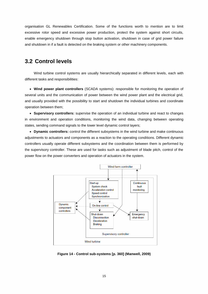
3.2 Control levels
Wind turbine control systems are usually hierarchically separated in different levels, each with
different tasks and responsibilities:
Wind power plant controllers (SCADA systems): responsible for monitoring the operation of
several units and the communication of power between the wind power plant and the electrical grid,
and usually provided with the possibility to start and shutdown the individual turbines and coordinate
operation between them;
Supervisory controllers: supervise the operation of an individual turbine and react to changes
in environment and operation conditions, monitoring the wind data, changing between operating
states, sending command signals to the lower level dynamic control layers;
Dynamic controllers: control the different subsystems in the wind turbine and make continuous
adjustments to actuators and components as a reaction to the operating conditions. Different dynamic
controllers usually operate different subsystems and the coordination between them is performed by
the supervisory controller. These are used for tasks such as adjustment of blade pitch, control of the
power flow on the power converters and operation of actuators in the system.
Figure 14 - Control sub-systems [p. 360] (Manwell, 2009)
16
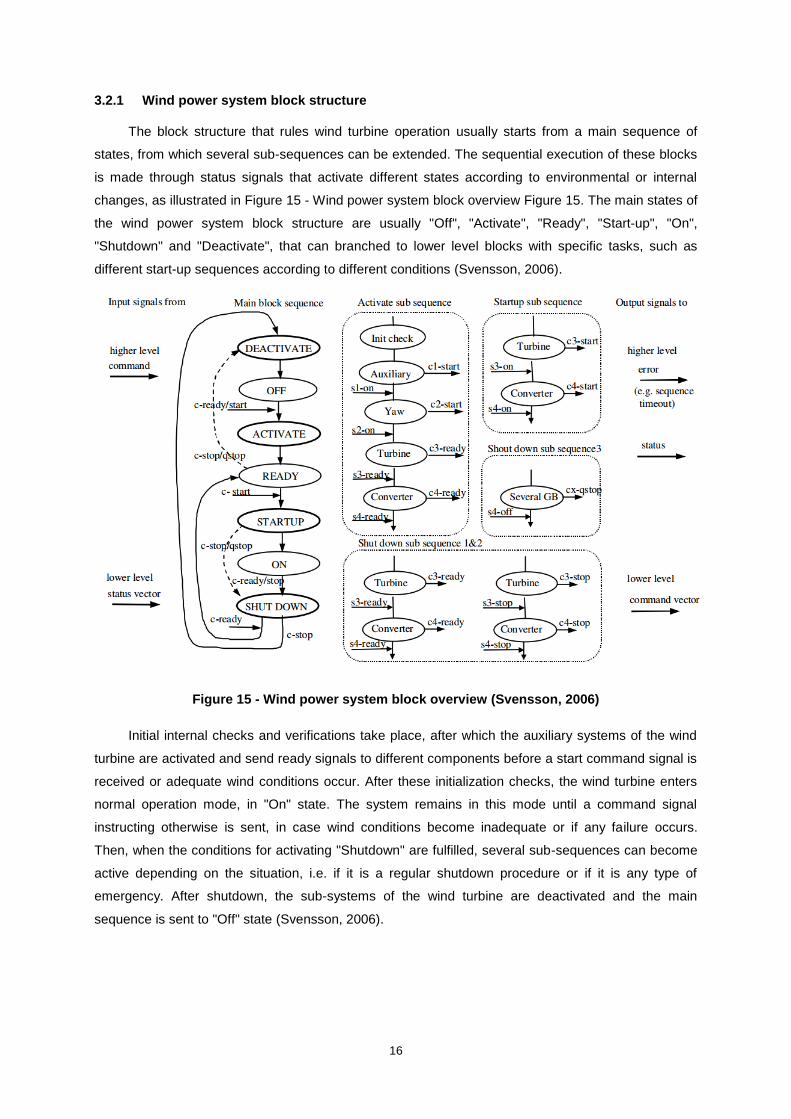
3.2.1 Wind power system block structure
The block structure that rules wind turbine operation usually starts from a main sequence of
states, from which several sub-sequences can be extended. The sequential execution of these blocks
is made through status signals that activate different states according to environmental or internal
changes, as illustrated in Figure 15 - Wind power system block overview Figure 15. The main states of
the wind power system block structure are usually "Off", "Activate", "Ready", "Start-up", "On",
"Shutdown" and "Deactivate", that can branched to lower level blocks with specific tasks, such as
different start-up sequences according to different conditions (Svensson, 2006).
Figure 15 - Wind power system block overview (Svensson, 2006)
Initial internal checks and verifications take place, after which the auxiliary systems of the wind
turbine are activated and send ready signals to different components before a start command signal is
received or adequate wind conditions occur. After these initialization checks, the wind turbine enters
normal operation mode, in "On" state. The system remains in this mode until a command signal
instructing otherwise is sent, in case wind conditions become inadequate or if any failure occurs.
Then, when the conditions for activating "Shutdown" are fulfilled, several sub-sequences can become
active depending on the situation, i.e. if it is a regular shutdown procedure or if it is any type of
emergency. After shutdown, the sub-systems of the wind turbine are deactivated and the main
sequence is sent to "Off" state (Svensson, 2006).
17
3.3 Variable speed control
The energy available in the wind varies continually as wind speed changes, which means that
the amount of power output that can be extracted from the wind is highly dependent on the accuracy
with which the maximum efficiency operating points are tracked by an effective optimum power
extraction strategy.
Wind turbines can be designed to work at a fixed or variable rotor speed. A fixed-speed wind
turbine operates always at roughly the same angular speed, which is dependent on the gearbox gear
ratio, the number of pole pairs of the generator and the grid electrical frequency. Such wind turbine
can only operate at maximum CP for one wind speed, to which corresponds the λopt. As the wind
speed varies from the optimal speed, λ varies along with it and the power coefficient decreases.
Several control strategies are used to vary the rotor speed and optimize or limit power output,
depending on whether the turbine is operating above or below rated wind speed. It is relevant to refer
some of the most used strategies:
Pitch control: Pitch regulation is mostly used in HAWT and consists in actively varying the
angle between the chord line of the blades and the rotor plane of rotation, i.e. the pitch angle β. This is
one of the most used control strategies in industry and enables an accurate control of power output.
Below rated power, the operation strategy is to operate in the CPmax curve and extract maximum
power. Whereas for operation above rated wind speeds, the blades can be rotated further into the
oncoming wind direction (furl) or away from the wind direction (stall) to change the aerodynamic forces
on the blades in order to decrease torque generation and consequently the power output (Manwell,
2009).
Stall control: A stall-regulated variable speed wind turbine has no pitch mechanism. The
control is performed by causing the blades to stall above a certain wind speed, reducing power output.
The angle of attack between the apparent wind speed (from Blade Element Momentum Theory) and
the plane of rotation is dependent on rotor speed. For further reading on BEM theory the reader can
refer to (Manwell, 2009).
Power control: Grid connected generators operate over a very small speed range and provide
the torque that is required to maintain operation at synchronous speed, so any mechanically imposed
torque results in almost instantaneous compensating torque. Alternatively, the generator can be
connected to the grid through an electronic power converter that allows the generator torque to be
very quickly set to any desired value. The converter determines the frequency, phase and voltage of
the current flowing from the generator, thus controlling the generator torque and rotational speed. This
is done by supplying the generator with a magnetization current ISG, setting a reference torque
(Manwell, 2009).

18
3.3.1 Synchronous machines
Synchronous machines are used as generators in large power plants, as well as in wind turbine
applications, usually installed in large grid-connected turbines or in conjunction with power electronic
converters in variable-speed wind turbines.
The synchronous generator consists of an AC machine with a magnetic source on the rotor that
rotates along with it and a stationary armature containing multiple windings. At steady state, the
rotation of the shaft, together with the number of pole pairs, defines the frequency of the supplied
current.
It is important to note though, without entering too much in electrical machine theoretical details,
that there is a constant angle between the rotor field and the resultant field, known as power angle,
which increases with torque. As long as the power angle is positive, the machine behaves as a
generator, however if the input torque drops, the power angle may become negative and the machine
will act as a motor (Manwell, 2009). Detailed discussion of electrical machine theory is outside the
scope of this work, so for a full development on this matter refer to (Fitzgerald, Jr., & Umans, 2003).
3.4 Maximum power extraction strategy
This section focuses on the control algorithm implemented for maximum power extraction from
the wind. Several control strategies to maximize energy yield could be applied. In the cases when the
power-rotor speed curve of the wind turbine is known, it is possible to control the power electronics
converter to deliver a predefined electric power as a function of the rotor speed ω to optimize power
extraction. However, this control strategy requires detailed knowledge of the Cp curve of the turbine
and the electrical machine parameters.
Since there is no trustworthy information about the electrical generator parameters or operation
curves for the wind turbine in this project, a different approach for achieving maximum power
generation is necessary.
3.4.1 Maximum Power Point Tracking methods
The purpose of a Maximum Power Point Tracking (MPPT) method is to maintain the tip-speed
ratio, λ, of the wind turbine as close as possible to the optimal tip-speed ratio, λopt, in order to achieve
maximum power extraction from the wind.
Three of the main control methods used for MPPT are Tip Speed Ratio control (TSR), Power
Signal Feedback control (PSF) and Hill-Climb Search (HCS) control also known as Perturbation and
Observation control (P&O). A brief overview of each method is provided in the following paragraphs.
19
The TSR control method consists in regulating the rotational speed of the generator in order to
keep the tip-speed ratio λ at the optimum level by knowing the value of the optimum speed ratio of the
turbine λopt. This method requires knowledge of both the wind speed and turbine speed, in addition to
the Cp curve of the wind turbine.
The PSF control method tracks the wind turbine's maximum power curve in order to extract
maximum power. The maximum power curve is obtained through simulation or offline experiment of
the turbine that is object of study. In this method, the reference power may be generated using the
values recorded for maximum power from experimental operation or by calculating the power through
the electrical power equation (equation 2 from section 2.3), with knowledge of the wind speed and
rotor speed.
The HCS control method acts by continuously searching for the peak power of the wind turbine,
using only measured data. For this tracking algorithm there is no need for information about the Cp
curve, optimum tip-speed ratio λopt or wind speed. This method verifies the location of the operating
point and establishes relations between the variations in power output and rotor speed to assess if the
rotor speed should be increased, decreased or maintained to drive the system to the point of
maximum power. Since it does not require prior knowledge of the maximum wind turbine power curve
nor of the electrical machine parameters, this method seems to be more advantageous comparing to
the previous ones for situations in which there is no reliable information about the wind turbine
operation. For a more detailed description about MPPT methods the reader should refer to (Thongam
& Ouhrouche, 2011).
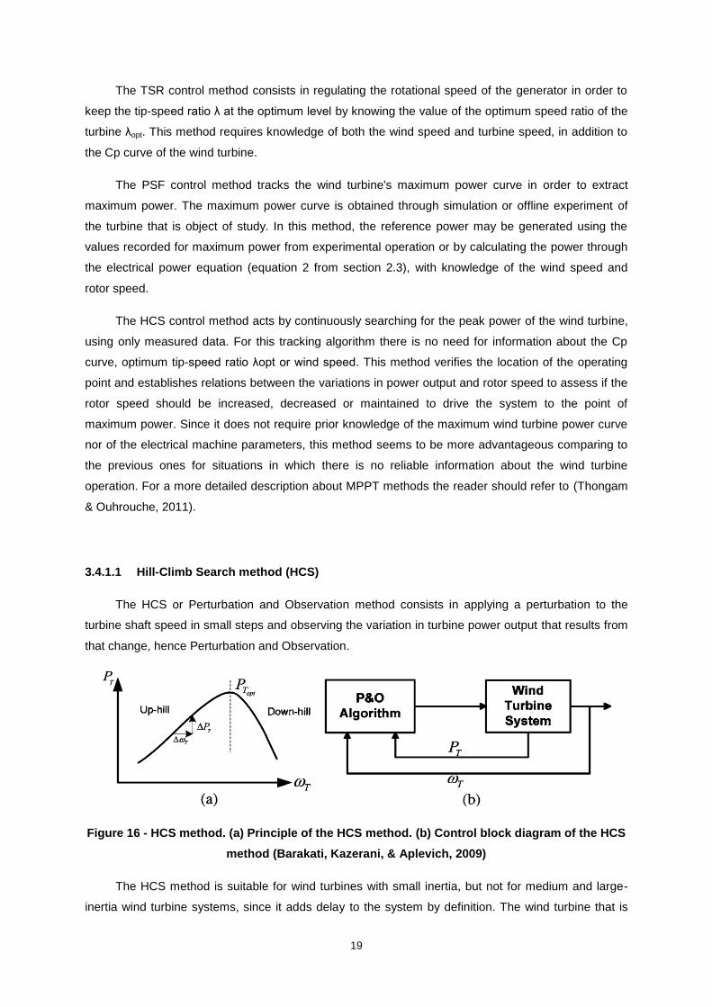
3.4.1.1 Hill-Climb Search method (HCS)
The HCS or Perturbation and Observation method consists in applying a perturbation to the
turbine shaft speed in small steps and observing the variation in turbine power output that results from
that change, hence Perturbation and Observation.
Figure 16 - HCS method. (a) Principle of the HCS method. (b) Control block diagram of the HCS
method (Barakati, Kazerani, & Aplevich, 2009)
The HCS method is suitable for wind turbines with small inertia, but not for medium and large-
inertia wind turbine systems, since it adds delay to the system by definition. The wind turbine that is
20
object of study in this project is assumed to be a small inertia setup, with its 2 meters rotor diameter
and relatively low inertia. For medium and large-inertia wind turbine systems, the turbine rotor has a
larger resistance to speed changes which adds a delay in response to wind speed variations and
prevents the HCS method from effectively control the wind turbine rotor speed. (Barakati, Kazerani, &
Aplevich, 2009).
The idea of this algorithm is to analyse the variation in power output resulting from a rotor speed
change and track the location of the optimal operating point. In Figure 16, the power curve can be
seen as an up-hill slope (ΔP>0) followed by a down-hill slope (ΔP<0), between which lies the point of
maximum power extraction.
Power control is performed by varying the current reference ISG in the synchronous generator
through power electronics. The generator side sets a torque reference that directly affects the wind
turbine rotor speed.
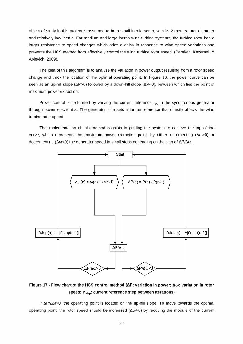
The implementation of this method consists in guiding the system to achieve the top of the
curve, which represents the maximum power extraction point, by either incrementing (Δω>0) or
decrementing (Δω<0) the generator speed in small steps depending on the sign of ΔP/Δω.
Figure 17 - Flow chart of the HCS control method (ΔP: variation in power; Δω: variation in rotor
speed; i*step: current reference step between iterations)
If ΔP/Δω>0, the operating point is located on the up-hill slope. To move towards the optimal
operating point, the rotor speed should be increased (Δω>0) by reducing the module of the current

21
reference ISG of the generator. Decreasing the load current ISG will reduce the electromagnetic torque
on the generator and consequently accelerate the wind turbine rotor.
If ΔP/Δω<0, the operating point is located on the down-hill slope, so the rotor speed should be
reduced (Δω<0) by increasing the synchronous generator current reference ISG in module, which
enhances the electromagnetic torque demand and thus decelerates the wind turbine rotor in order to
extract more power from the mechanical rotation.
If incrementing the shaft speed results in ΔP/Δω<0 or decrementing the shaft speed results in
ΔP/Δω>0, the signal of the shaft speed variation must be reversed. This perturbation and observation
routine is repeated iteratively, until the point where ΔP/Δω=0 is reached and maximum power
extraction is achieved. In practice, the exact maximum efficiency point is not kept constant, but rather
approximated by small steps in rotor speed change around the optimal operating point. The algorithm
that rules this control method is briefly summarized as follows:
Impose small variation in rotor speed, e.g. Δω>0 (Perturbation)
Verify if the output power is increasing or decreasing (Observation)
o Power decreasing:
Rotor speed was increasing:
Reduce rotor speed: Increase the load current ISG
Rotor speed was decreasing:
Increase rotor speed: Reduce the load current ISG
o Power increasing:
Rotor speed was increasing:
Increase rotor speed: Reduce the load current ISG
Rotor speed was decreasing:
Reduce rotor speed: Increase the load current ISG
22
4 LTH Wind Turbine unit
4.1 Intended functions
By having an experimental wind turbine setup of its own, the IEA (Industrial Electrical
Engineering and Automation) department can use it to test different experimental devices and
software, such as generators or data acquisition and control systems. It is intended to study the
behaviour of the wind turbine and be able to relate the setup to large scale power production systems,
such as offshore wind power plants or multi source renewable energy setups. Thus, the modularity of
the system is anticipating future expansion of the production site by adding new generation units.
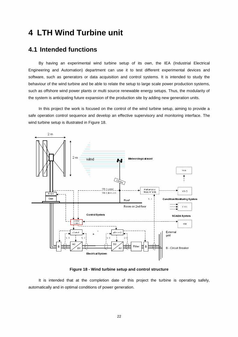
In this project the work is focused on the control of the wind turbine setup, aiming to provide a
safe operation control sequence and develop an effective supervisory and monitoring interface. The
wind turbine setup is illustrated in Figure 18.
Figure 18 - Wind turbine setup and control structure
It is intended that at the completion date of this project the turbine is operating safely,
automatically and in optimal conditions of power generation.
B - Circuit Breaker

23
The specific goals of the implementation are:
Guarantee the safety of the setup and the university surroundings by constantly monitoring
the rotor speed to avoid hazardous situations in case of strong winds;
Inform the operator of any irregular situations related to the power converters, generator
voltage, current or the DC connection, and react accordingly;
Provide the operator with the possibility of stopping the wind turbine through a mechanical
brake, in case of emergency;
Apply the brake automatically in case of power failure to prevent the turbine from rotating
in 'freewheel', which could accelerate the rotor to dangerous speeds for which the structure is not
prepared and thus increase the probability of accidents;
Brake the turbine automatically in case the wind speed exceeds a maximum value (cut-out
wind speed);
Implement a control algorithm in order to extract the maximum amount of energy from the
wind;
Allow the operator to select the desired mode of operation.
The power production unit installed consists of a vertical axis wind turbine that feeds a
permanent magnet synchronous generator, which is connected to the electrical grid through an
AC/DC/AC connection with two power converters, i.e. a rectifier, DC-link and inverter. The following
sections provide an overview of the components of the system to present the elements with which the
control system will interact.
4.2 Control structure
The control system is distributed in two levels: control of the power converters through two
microcontrollers and overall control that performs high level control tasks on the setup.
Communication between the two levels provides the main control with information about the power
converters and real-time voltage and current measurements or error signals.
The setup consists of a vertical axis wind turbine equipped with a permanent magnet
synchronous generator and a mechanical drum brake, a meteorological mast where wind speed, wind
direction, air pressure and temperature are measured, a camera for monitoring the operation of the
wind turbine and two cabinets located in a room below the WT setup that contain the power converters
and the microcontrollers (Figure 18).
The overall control is the object of study in this project. The main objective is to develop and
implement a solution to perform high level control tasks on the system. The overall control is
responsible for managing the internal functions of the system, establish a control sequence to guide
the WT through the different states of operation, manage the occurrence of errors and provide an
adapted response to different situations. It is designed to be a modular element that does not need to
be embedded in the turbine setup to be implemented as a high level power-plant control unit.
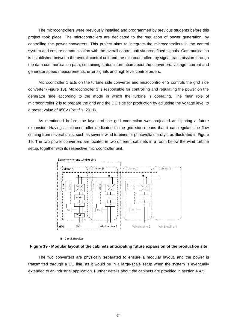
24
The microcontrollers were previously installed and programmed by previous students before this
project took place. The microcontrollers are dedicated to the regulation of power generation, by
controlling the power converters. This project aims to integrate the microcontrollers in the control
system and ensure communication with the overall control unit via predefined signals. Communication
is established between the overall control unit and the microcontrollers by signal transmission through
the data communication path, containing status information about the converters, voltage, current and
generator speed measurements, error signals and high level control orders.
Microcontroller 1 acts on the turbine side converter and microcontroller 2 controls the grid side
converter (Figure 18). Microcontroller 1 is responsible for controlling and regulating the power on the
generator side according to the mode in which the turbine is operating. The main role of
microcontroller 2 is to prepare the grid and the DC side for production by adjusting the voltage level to
a preset value of 450V (Petitfils, 2011).
As mentioned before, the layout of the grid connection was projected anticipating a future
expansion. Having a microcontroller dedicated to the grid side means that it can regulate the flow
coming from several units, such as several wind turbines or photovoltaic arrays, as illustrated in Figure
19. The two power converters are located in two different cabinets in a room below the wind turbine
setup, together with its respective microcontroller unit.
Figure 19 - Modular layout of the cabinets anticipating future expansion of the production site
The two converters are physically separated to ensure a modular layout, and the power is
transmitted through a DC line, as it would be in a large-scale setup when the system is eventually
extended to an industrial application. Further details about the cabinets are provided in section 4.4.5.
B - Circuit Breaker
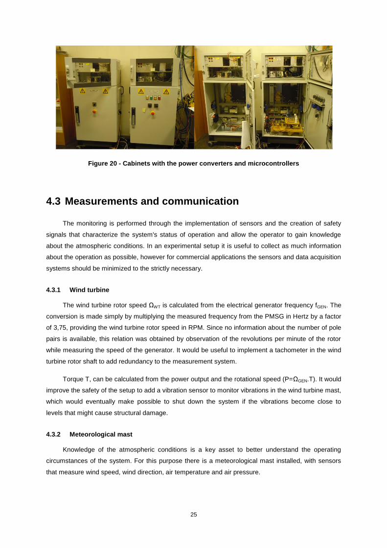
25
Figure 20 - Cabinets with the power converters and microcontrollers
4.3 Measurements and communication
The monitoring is performed through the implementation of sensors and the creation of safety
signals that characterize the system's status of operation and allow the operator to gain knowledge
about the atmospheric conditions. In an experimental setup it is useful to collect as much information
about the operation as possible, however for commercial applications the sensors and data acquisition
systems should be minimized to the strictly necessary.
4.3.1 Wind turbine
The wind turbine rotor speed ΩWT is calculated from the electrical generator frequency fGEN. The
conversion is made simply by multiplying the measured frequency from the PMSG in Hertz by a factor
of 3,75, providing the wind turbine rotor speed in RPM. Since no information about the number of pole
pairs is available, this relation was obtained by observation of the revolutions per minute of the rotor
while measuring the speed of the generator. It would be useful to implement a tachometer in the wind
turbine rotor shaft to add redundancy to the measurement system.
Torque T, can be calculated from the power output and the rotational speed (P=ΩGEN.T). It would
improve the safety of the setup to add a vibration sensor to monitor vibrations in the wind turbine mast,
which would eventually make possible to shut down the system if the vibrations become close to
levels that might cause structural damage.
4.3.2 Meteorological mast
Knowledge of the atmospheric conditions is a key asset to better understand the operating
circumstances of the system. For this purpose there is a meteorological mast installed, with sensors
that measure wind speed, wind direction, air temperature and air pressure.

26
The wind speed is measured by an anemometer and directly connected to the control system,
where it is decoded and used in the state sequence. The wind direction is obtained analogously.
Pressure and temperature are measured and the signals are connected to the weather station's data
logger and can be downloaded via FTP communication with an embedded web-server at a defined
rate.
4.3.3 Safety signals
The power electronics control implementation has a set of safety signals that assure that the
converters are being regulated properly. These signals are triggered in the eventuality of system
failure or component malfunction, informing the system of the fault or enabling an automatic reaction if
that is the case. These safety signals alert for:
Inverter error;
Low voltage;
High voltage;
High current;
High current (DC link).
The mechanical brake is activated via a logic signal sent by the control system that physically
brakes the wind turbine shaft in the eventuality of an emergency shutdown or is applied for safety
when the turbine is shut down and motionless.
4.4 Technical specifications
4.4.1 Wind turbine
Technical Specifications
Manufacturer/model EXAMEC / 1,8 kW
Rotor diameter 2 m
Rotor height 2 m
Mast height 6 m
Tower type Tubular
Rated power 1,8 kW
Rated wind speed 12 m/s (not confirmed)
Rotor speed range 0-240 rpm (not confirmed)
Fixed or variable pitch No pitch control
Number of blades 3
Table 1- Wind turbine technical specifications
The wind turbine installed on the roof top of the university is a vertical-axis turbine designed and
manufactured by EXAMEC, a Swedish manufacturer of high precision engineering components. It has
a 2 meter rotor diameter, three 2 meter long blades and no option for pitch control, hence the control
of the wind turbine is accomplished with power electronics to adjust the synchronous generator
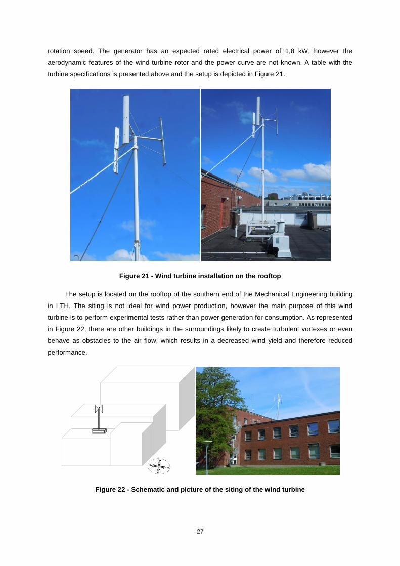
27
rotation speed. The generator has an expected rated electrical power of 1,8 kW, however the
aerodynamic features of the wind turbine rotor and the power curve are not known. A table with the
turbine specifications is presented above and the setup is depicted in Figure 21.
Figure 21 - Wind turbine installation on the rooftop
The setup is located on the rooftop of the southern end of the Mechanical Engineering building
in LTH. The siting is not ideal for wind power production, however the main purpose of this wind
turbine is to perform experimental tests rather than power generation for consumption. As represented
in Figure 22, there are other buildings in the surroundings likely to create turbulent vortexes or even
behave as obstacles to the air flow, which results in a decreased wind yield and therefore reduced
performance.
Figure 22 - Schematic and picture of the siting of the wind turbine
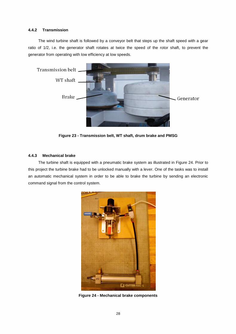
28
4.4.2 Transmission
The wind turbine shaft is followed by a conveyor belt that steps up the shaft speed with a gear
ratio of 1/2, i.e. the generator shaft rotates at twice the speed of the rotor shaft, to prevent the
generator from operating with low efficiency at low speeds.
Figure 23 - Transmission belt, WT shaft, drum brake and PMSG
4.4.3 Mechanical brake
The turbine shaft is equipped with a pneumatic brake system as illustrated in Figure 24. Prior to
this project the turbine brake had to be unlocked manually with a lever. One of the tasks was to install
an automatic mechanical system in order to be able to brake the turbine by sending an electronic
command signal from the control system.
Figure 24 - Mechanical brake components
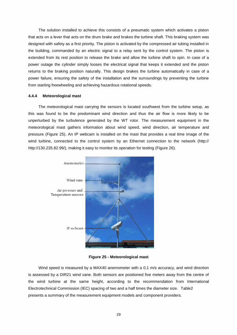
29
The solution installed to achieve this consists of a pneumatic system which activates a piston
that acts on a lever that acts on the drum brake and brakes the turbine shaft. This braking system was
designed with safety as a first priority. The piston is activated by the compressed air tubing installed in
the building, commanded by an electric signal to a relay sent by the control system. The piston is
extended from its rest position to release the brake and allow the turbine shaft to spin. In case of a
power outage the cylinder simply looses the electrical signal that keeps it extended and the piston
returns to the braking position naturally. This design brakes the turbine automatically in case of a
power failure, ensuring the safety of the installation and the surroundings by preventing the turbine
from starting freewheeling and achieving hazardous rotational speeds.
4.4.4 Meteorological mast
The meteorological mast carrying the sensors is located southwest from the turbine setup, as
this was found to be the predominant wind direction and thus the air flow is more likely to be
unperturbed by the turbulence generated by the WT rotor. The measurement equipment in the
meteorological mast gathers information about wind speed, wind direction, air temperature and
pressure (Figure 25). An IP webcam is installed on the mast that provides a real time image of the
wind turbine, connected to the control system by an Ethernet connection to the network (http://
http://130.235.82.99/), making it easy to monitor its operation for testing (Figure 26).
Figure 25 - Meteorological mast
Wind speed is measured by a MAX40 anemometer with a 0,1 m/s accuracy, and wind direction
is assessed by a DIR21 wind vane. Both sensors are positioned five meters away from the centre of
the wind turbine at the same height, according to the recommendation from International
Electrotechnical Commission (IEC) spacing of two and a half times the diameter size. Table2
presents a summary of the measurement equipment models and component providers.
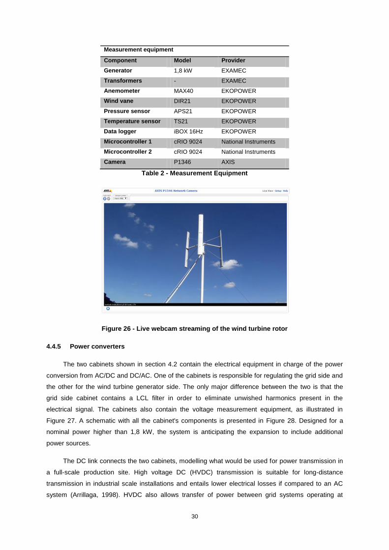
30
Measurement equipment
Component Model Provider
Generator 1,8 kW EXAMEC
Transformers - EXAMEC
Anemometer MAX40 EKOPOWER
Wind vane DIR21 EKOPOWER
Pressure sensor APS21 EKOPOWER
Temperature sensor TS21 EKOPOWER
Data logger iBOX 16Hz EKOPOWER
Microcontroller 1 cRIO 9024 National Instruments
Microcontroller 2 cRIO 9024 National Instruments
Camera P1346 AXIS
Table 2 - Measurement Equipment
Figure 26 - Live webcam streaming of the wind turbine rotor
4.4.5 Power converters
The two cabinets shown in section 4.2 contain the electrical equipment in charge of the power
conversion from AC/DC and DC/AC. One of the cabinets is responsible for regulating the grid side and
the other for the wind turbine generator side. The only major difference between the two is that the
grid side cabinet contains a LCL filter in order to eliminate unwished harmonics present in the
electrical signal. The cabinets also contain the voltage measurement equipment, as illustrated in
Figure 27. A schematic with all the cabinet's components is presented in Figure 28. Designed for a
nominal power higher than 1,8 kW, the system is anticipating the expansion to include additional
power sources.
The DC link connects the two cabinets, modelling what would be used for power transmission in
a full-scale production site. High voltage DC (HVDC) transmission is suitable for long-distance
transmission in industrial scale installations and entails lower electrical losses if compared to an AC
system (Arrillaga, 1998). HVDC also allows transfer of power between grid systems operating at
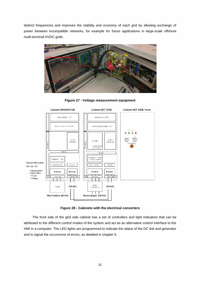
31
distinct frequencies and improves the stability and economy of each grid by allowing exchange of
power between incompatible networks, for example for future applications in large-scale offshore
multi-terminal HVDC grids.
Figure 27 - Voltage measurement equipment
Figure 28 - Cabinets with the electrical converters
The front side of the grid side cabinet has a set of controllers and light indicators that can be
attributed to the different control modes of the system and act as an alternative control interface to the
HMI in a computer. The LED lights are programmed to indicate the status of the DC link and generator
and to signal the occurrence of errors, as detailed in chapter 5.

32
4.5 Automation equipment and engineering tools
The characteristics of the control system that this project aimed to develop require data
acquisition and manipulation from the measurement systems (both meteorological and electrical),
signal communication with reliability and at high speeds to ensure performance and flexibility of
programming since this is an experimental setup suitable to be upgraded and changed.
LabVIEW is a widely spread engineering tool throughout the industry and it is an adequate
solution for the implementation. The following section explains its relevance in the project and
provides the reader with an overview of its capabilities as well as the hardware where it is
implemented. This overview was thought to be of importance in order to understand the
implementation described in chapter 5.5.
4.5.1 Programming in LabVIEW
NI LabVIEW is a graphical programming environment and system design platform from National
Instruments. It is widely used throughout the industry as an engineering tool for the development of
sophisticated control systems implemented in a wide variety of applications. It is a high-level
programming language, adequate for applications that require real-world data acquisition and
manipulation, file input/output (I/O) and industrial automation, among many other uses, without the
need of dealing with the smaller programming details of lower-level languages.
It enables engineers to develop effective solutions without the necessity of profound low-level
programming skills, by dragging and dropping the desired virtual representations of laboratory
equipment on the LabVIEW environment. However, it is compatible with C++ and other languages,
making it flexible to satisfy the user's needs according to its programming skills. It consists of a
dataflow programming platform, resembling a flowchart composed of icons and wires, which execution
sequence is determined by the structure of the block diagram, with inherent capacity for multi-
processing and multi-threading. Since it allows parallel execution, LabVIEW is adequate to program
using parallel events and thus make the code easier to read and display, comparing to traditional
sequential textual programming languages.
LabVIEW is extensively equipped with libraries for data acquisition, signal generation, signal
conditioning, advanced control and data visualization that are suitable to interact with a wide range of
hardware developed by NI (NI, Developer's Guide, 2013).
LabVIEW's programs or subroutines are called Virtual Instruments (VI), in which the functions,
structures, controls and indicators are created and displayed. Each VI is constituted by a block
diagram, a front panel and a connector panel. The source code is implemented in the form of a block
diagram, where indicators and controls are presented in a customizable front panel, while the
connector panel is used to represent the connections and interactions between different VI's.
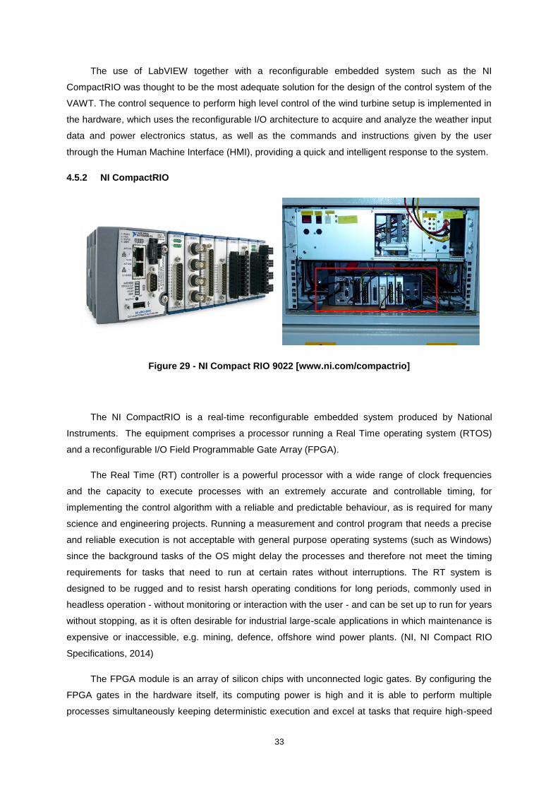
33
The use of LabVIEW together with a reconfigurable embedded system such as the NI
CompactRIO was thought to be the most adequate solution for the design of the control system of the
VAWT. The control sequence to perform high level control of the wind turbine setup is implemented in
the hardware, which uses the reconfigurable I/O architecture to acquire and analyze the weather input
data and power electronics status, as well as the commands and instructions given by the user
through the Human Machine Interface (HMI), providing a quick and intelligent response to the system.
4.5.2 NI CompactRIO
Figure 29 - NI Compact RIO 9022 [www.ni.com/compactrio]
The NI CompactRIO is a real-time reconfigurable embedded system produced by National
Instruments. The equipment comprises a processor running a Real Time operating system (RTOS)
and a reconfigurable I/O Field Programmable Gate Array (FPGA).
The Real Time (RT) controller is a powerful processor with a wide range of clock frequencies
and the capacity to execute processes with an extremely accurate and controllable timing, for
implementing the control algorithm with a reliable and predictable behaviour, as is required for many
science and engineering projects. Running a measurement and control program that needs a precise
and reliable execution is not acceptable with general purpose operating systems (such as Windows)
since the background tasks of the OS might delay the processes and therefore not meet the timing
requirements for tasks that need to run at certain rates without interruptions. The RT system is
designed to be rugged and to resist harsh operating conditions for long periods, commonly used in
headless operation - without monitoring or interaction with the user - and can be set up to run for years
without stopping, as it is often desirable for industrial large-scale applications in which maintenance is
expensive or inaccessible, e.g. mining, defence, offshore wind power plants. (NI, NI Compact RIO
Specifications, 2014)
The FPGA module is an array of silicon chips with unconnected logic gates. By configuring the
FPGA gates in the hardware itself, its computing power is high and it is able to perform multiple
processes simultaneously keeping deterministic execution and excel at tasks that require high-speed

34
logic operations. It is directly connected to the I/O modules, from which data is acquired into the I/O
circuitry almost without control latency or jitter and with high performance. Because the FPGA runs all
code in hardware, it provides high reliability and determinism, with custom timing and high-speed
acquisition. The I/O modules are chosen to suit the user's needs from a wide range of models and
wiring options to connect sensors, actuators, accelerometers, signal processors, power measurement
equipment and all kinds of analogical and digital input/output. The signals are then processed using
LabVIEW. (NI, NI Compact RIO Specifications, 2014)
4.5.3 NI Compact RIOs in the control system:
Two Compact RIOs are connected to the sensors used in the measurement process and convert
the sensor signals to digital data to be monitored, analyzed and recorded. They have communication
capabilities to report the status of the system to the human interface that works as a supervisory
system, and also to receive commands from the user to be applied in the system in real time. Further
explanations on the system architecture are provided in section 5.2.
The Compact RIOs used for the implementation of the control system grant great flexibility to the
experimental setup. As this VAWT system is installed for experimental purposes, it is intended to have
extensive data acquisition and monitoring. However, once the algorithm is implemented and fully
operational, the control system could be simplified and approximated to a commercial installation by
reducing the amount of measurements to the strictly necessary for regular operation monitoring. In this
case, it would be adequate to transfer the control program to e.g. an embedded system like a single
board RIO in order to install it as a standard unit, cheaper and tailored to the needs of the algorithm
and code.
The modules installed in the Compact RIOs on the laboratorial setup are:
NI 9205 (32 terminal Analog Input)
NI 9215 (+/- Input Analog terminals)
NI 9263 (4-Channel, +-10V, 16 Bit Analog Output)
NI 9474 (8-Channel Digital Output)
NI 9401 (8-Channel, TTL Digital Input/Output).
4.5.4 CompactRIO VS myRIO
The NI myRIO was considered as an option for the implementation of the overall control code,
although it has been decided for the Compact RIO instead. The myRIO is an academic learning
module, an affordable tool intended to be used by engineering students for small projects and simple
applications, and was thought perhaps not to have enough memory for the operations that will be
performed. However, this is an option to consider in further works in order to have the overall control
program in a separate device rather than embedded in one of the two microcontrollers as it is now. For
further details on the system architecture refer to chapter 5.

35
5 Control implementation
5.1 Control requirements
The aim of the work is to ensure the safety of the installation and allow the system to operate
automatically for an extended period of time, fulfilling the control requirements detailed in section 4.1.
The overall control system of the installation is responsible for:
Monitoring the internal operating conditions;
Operating the wind turbine on an automatic and sequential way;
Navigating through the state sequence that composes the wind power system block
structure;
Acquiring signals from the wind conditions measurements and analysing the data;
Allowing the operator to interact with the system to start and stop the generation unit;
Allowing the operator to elect the control mode the turbine will be operating on;
Allowing different modes for start-up and shutdown;
Establishing a remote panel interface to allow communication with Vattenhallen for
demonstration purposes.
This chapter describes the architecture of the system and the way how the different
components interact, presents the control sequence designed for the wind turbine system and its
operation modes of production, and finally an explanation of the programming in LabVIEW is provided.
5.2 System architecture
The control structure is represented in Figure 30:
Figure 30 - Wind turbine setup and control structure
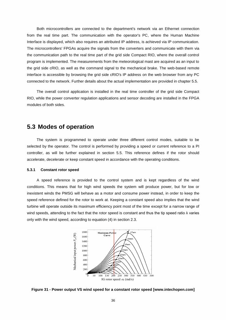
36
Both microcontrollers are connected to the department's network via an Ethernet connection
from the real time part. The communication with the operator's PC, where the Human Machine
Interface is displayed, which also requires an attributed IP address, is achieved via IP communication.
The microcontrollers' FPGAs acquire the signals from the converters and communicate with them via
the communication path to the real time part of the grid side Compact RIO, where the overall control
program is implemented. The measurements from the meteorological mast are acquired as an input to
the grid side cRIO, as well as the command signal to the mechanical brake. The web-based remote
interface is accessible by browsing the grid side cRIO's IP address on the web browser from any PC
connected to the network. Further details about the actual implementation are provided in chapter 5.5.
The overall control application is installed in the real time controller of the grid side Compact
RIO, while the power converter regulation applications and sensor decoding are installed in the FPGA
modules of both sides.
5.3 Modes of operation
The system is programmed to operate under three different control modes, suitable to be
selected by the operator. The control is performed by providing a speed or current reference to a PI
controller, as will be further explained in section 5.5. This reference defines if the rotor should
accelerate, decelerate or keep constant speed in accordance with the operating conditions.
5.3.1 Constant rotor speed
A speed reference is provided to the control system and is kept regardless of the wind
conditions. This means that for high wind speeds the system will produce power, but for low or
inexistent winds the PMSG will behave as a motor and consume power instead, in order to keep the
speed reference defined for the rotor to work at. Keeping a constant speed also implies that the wind
turbine will operate outside its maximum efficiency point most of the time except for a narrow range of
wind speeds, attending to the fact that the rotor speed is constant and thus the tip speed ratio λ varies
only with the wind speed, according to equation (4) in section 2.3.
Figure 31 - Power output VS wind speed for a constant rotor speed [www.intechopen.com]
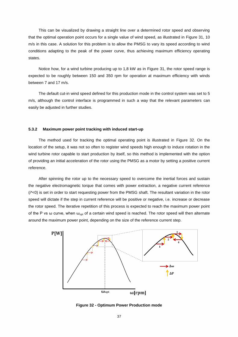
37
This can be visualized by drawing a straight line over a determined rotor speed and observing
that the optimal operation point occurs for a single value of wind speed, as illustrated in Figure 31, 10
m/s in this case. A solution for this problem is to allow the PMSG to vary its speed according to wind
conditions adapting to the peak of the power curve, thus achieving maximum efficiency operating
states.
Notice how, for a wind turbine producing up to 1,8 kW as in Figure 31, the rotor speed range is
expected to be roughly between 150 and 350 rpm for operation at maximum efficiency with winds
between 7 and 17 m/s.
The default cut-in wind speed defined for this production mode in the control system was set to 5
m/s, although the control interface is programmed in such a way that the relevant parameters can
easily be adjusted in further studies.
5.3.2 Maximum power point tracking with induced start-up
The method used for tracking the optimal operating point is illustrated in Figure 32. On the
location of the setup, it was not so often to register wind speeds high enough to induce rotation in the
wind turbine rotor capable to start production by itself, so this method is implemented with the option
of providing an initial acceleration of the rotor using the PMSG as a motor by setting a positive current
reference.
After spinning the rotor up to the necessary speed to overcome the inertial forces and sustain
the negative electromagnetic torque that comes with power extraction, a negative current reference
(i*<0) is set in order to start requesting power from the PMSG shaft. The resultant variation in the rotor
speed will dictate if the step in current reference will be positive or negative, i.e. increase or decrease
the rotor speed. The iterative repetition of this process is expected to reach the maximum power point
of the P vs ω curve, when ωopt of a certain wind speed is reached. The rotor speed will then alternate
around the maximum power point, depending on the size of the reference current step.
Figure 32 - Optimum Power Production mode

38
Since the initial rotation is provided by the motor, the cut-in wind speed defined for this mode is
the same as for constant speed mode, 5 m/s. This parameter is also suitable to be changed by the
operator.
For ease of understanding, the algorithm that rules this control method is once again provided
below:
Impose small variation in rotor speed, e.g. Δω>0 (Perturbation)
Verify if the output power is increasing or decreasing (Observation)
o Power decreasing:
Rotor speed was increasing:
Reduce rotor speed: Increase the load current ISG
Rotor speed was decreasing:
Increase rotor speed: Reduce the load current ISG
o Power increasing:
Rotor speed was increasing:
Increase rotor speed: Reduce the load current ISG
Rotor speed was decreasing:
Reduce rotor speed: Increase the load current ISG
5.3.3 Maximum power point tracking with freewheeling start-up
Although lift actuated VAWTs are usually not capable of self-starting, it is intended to include this
option for experimentation and as a way of gaining more knowledge about the turbine capabilities. The
implementation of this method is exactly the same as the one described previously, with the difference
that the initial rotation is created by the wind speed itself rather than by the motor. This mode is
expected to be viable only for high wind speeds, since in previous observations the rotor barely seems
to start freewheeling for wind speeds up to 7 m/s, moreover it needs to accelerate to a high enough
rotational speed to start production, as explained in the previous section. Therefore, the default cut-in
wind speed for this mode was set at 8 m/s.
5.4 Plant system block structure
The control sequence of the wind turbine system is designed as a state machine diagram,
consisting of a sequence of states in which actions are applied to the system, separated by
predetermined transition conditions. The transitions between states are triggered by command signals
or specifically defined operating conditions as shown in Figure 33.
The main sequence is presented on the left side of Figure 33, where the main states are set,
according to the theory in the sources referred in chapter 3. The main states of operation are OFF,
ACTIVATE, READY, START UP, ON, SHUTDOWN and DEACTIVATE. Some sub-sequences are
extended from the high-level blocks START UP, SHUTDOWN and DEACTIVATE, because generally
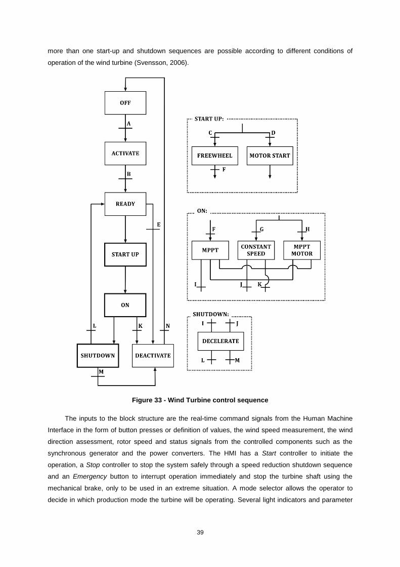
39
more than one start-up and shutdown sequences are possible according to different conditions of
operation of the wind turbine (Svensson, 2006).
Figure 33 - Wind Turbine control sequence
The inputs to the block structure are the real-time command signals from the Human Machine
Interface in the form of button presses or definition of values, the wind speed measurement, the wind
direction assessment, rotor speed and status signals from the controlled components such as the
synchronous generator and the power converters. The HMI has a Start controller to initiate the
operation, a Stop controller to stop the system safely through a speed reduction shutdown sequence
and an Emergency button to interrupt operation immediately and stop the turbine shaft using the
mechanical brake, only to be used in an extreme situation. A mode selector allows the operator to
decide in which production mode the turbine will be operating. Several light indicators and parameter
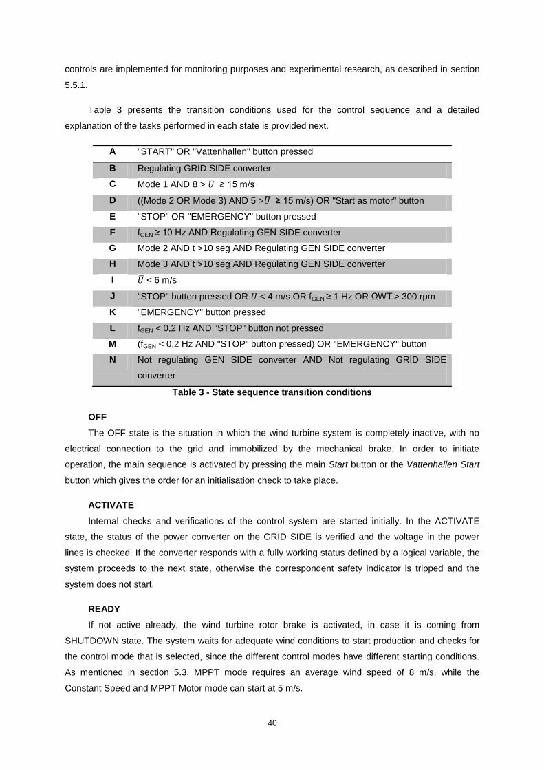
40
controls are implemented for monitoring purposes and experimental research, as described in section
5.5.1.
Table 3 presents the transition conditions used for the control sequence and a detailed
explanation of the tasks performed in each state is provided next.
A "START" OR "Vattenhallen" button pressed
B Regulating GRID SIDE converter
C Mode 1 AND 8 > ≥ 15 m/s
D ((Mode 2 OR Mode 3) AND 5 > ≥ 15 m/s) OR "Start as motor" button
E "STOP" OR "EMERGENCY" button pressed
F fGEN ≥ 10 Hz AND Regulating GEN SIDE converter
G Mode 2 AND t >10 seg AND Regulating GEN SIDE converter
H Mode 3 AND t >10 seg AND Regulating GEN SIDE converter
I < 6 m/s
J "STOP" button pressed OR < 4 m/s OR fGEN ≥ 1 Hz OR ΩWT > 300 rpm
K "EMERGENCY" button pressed
L fGEN < 0,2 Hz AND "STOP" button not pressed
M (fGEN < 0,2 Hz AND "STOP" button pressed) OR "EMERGENCY" button
N Not regulating GEN SIDE converter AND Not regulating GRID SIDE
converter
Table 3 - State sequence transition conditions
OFF
The OFF state is the situation in which the wind turbine system is completely inactive, with no
electrical connection to the grid and immobilized by the mechanical brake. In order to initiate
operation, the main sequence is activated by pressing the main Start button or the Vattenhallen Start
button which gives the order for an initialisation check to take place.
ACTIVATE
Internal checks and verifications of the control system are started initially. In the ACTIVATE
state, the status of the power converter on the GRID SIDE is verified and the voltage in the power
lines is checked. If the converter responds with a fully working status defined by a logical variable, the
system proceeds to the next state, otherwise the correspondent safety indicator is tripped and the
system does not start.
READY
If not active already, the wind turbine rotor brake is activated, in case it is coming from
SHUTDOWN state. The system waits for adequate wind conditions to start production and checks for
the control mode that is selected, since the different control modes have different starting conditions.
As mentioned in section 5.3, MPPT mode requires an average wind speed of 8 m/s, while the
Constant Speed and MPPT Motor mode can start at 5 m/s.

41
The sequence is set to proceed if the average wind speed is between 5 and 15 m/s. Below this
cut-in wind speed the wind turbine has no capacity to produce power, and for safety reasons the
production is interrupted in case the wind exceeds the cut-out threshold. For experimental purposes,
this wind speed limitation can be overruled by pressing the Start as motor button, which will initiate the
PMSG as a motor regardless of the wind speed. If at any time the STOP or EMERGENCY buttons are
pressed, the system proceeds to DEACTIVATE state.
Before initiating power production, the turbine must be rotating at a minimum speed to overcome
the electromagnetic torque imposed by the synchronous generator.
START-UP
To achieve this, the turbine is either accelerated using the PMSG as a motor (MOTOR START)
or, if the wind is blowing at a sufficiently high speed, by releasing the brake and letting the rotor start
spinning in FREEWHEEL until a threshold rotational speed is reached.
Constant Speed and MPPT Motor modes require to be started as a motor. The MOTOR START
block verifies that the generator side converter is activated and working properly and then it will
accelerate the rotor for 10 seconds to gain speed. MPPT mode will pick up speed from the wind until a
generator frequency fGEN of 10 Hz is reached.
ON
The wind turbine is in normal operation mode when reaching the ON state. This implies that the
system is prepared to run in one of the three different control modes:
MPPT: if the average wind speed drops below 6 m/s, the system proceeds to READY;
Constant Speed: if the average wind speed drops below 4 m/s, the system proceeds to
READY;
MPPT Motor: if the average wind speed drops below 4 m/s, the system proceeds to READY;
In all three modes production can be intentionally interrupted by pressing the Stop button which
leads to a gradual deceleration of the rotor in the SHUTDOWN state, or immediately stopped by
pressing the Emergency button that sends the system into DEACTIVATE state. If for any other reason
the generator frequency falls below a threshold level of 1 Hz, the system goes back to READY state. If
the rotor speed accelerates up to a threshold limit defined by default at 300 rpm, which might mean
that the system went out of control, the state sequence proceeds to SHUTDOWN.
SHUTDOWN
If the system is intended to be stopped in normal conditions, the generator rotor is gradually
decelerated through power electronics to a full stop, and then proceeds to be deactivated. This block
verifies whether the Stop button has been pressed or not and proceeds to READY or DEACTIVATE
state accordingly. When the generator frequency drops below 0,2 Hz, it is safe to apply the
mechanical brake and fully immobilize the shaft.

42
DEACTIVATE
This state is reached either after a gradual shutdown or an emergency situation where the
system needs to be stopped immediately by pressing the Emergency button. This stop mode is not
advisable to be used unless in extreme situations, since an abrupt stop of the spinning rotor shaft
using the mechanical brake can cause damage both to the mechanical and electrical system,
especially if the turbine is rotating at high speeds.
The mechanical brake is locked in, and the power converters stop being regulated sequentially -
first the generator side converter, and after confirmation of its deactivation without errors, the grid side
converter is safely disconnected and the system is turned OFF.
After describing the control sequence in respect to which the system operates, it is pertinent to
present the programming features and strategies that were implemented in order to bring this to reality
in the wind turbine setup.
5.5 LabVIEW implementation
The focus of this project was to implement the high-level control that supervises and manages all
the variables and inputs to monitor the system operation and provide an adequate response to
dynamic variations. This section describes and explains the LabVIEW code developed to achieve this.
The overall control application is installed on the real time controller, while the power converters
regulation and the wind measurements are performed in the FPGA module.
Prior to this project, the two microcontrollers that regulate the power converters had been
previously programmed to measure and regulate the grid side and generator side voltage and current
with a phase locked loop (PLL) to calculate the frequency and pulse width modulation (PWM).
Two controllers to regulate the generator speed are implemented in the FPGA of the generator
side microcontroller: a current PI controller and a speed P controller. The current control is performed
by providing the current set-point to the PID block in LabVIEW in both the x and y coordinates in the
rotor frame reference (ix* and iy*). The current reference can be set manually or calculated in the
speed PID block, depending on the regulating mode (Figure 34). The speed PID basically creates a
current reference based on the generator speed set-point (speed*[Hz]) and feeds it to the current
controller, as Figure 35 shows.
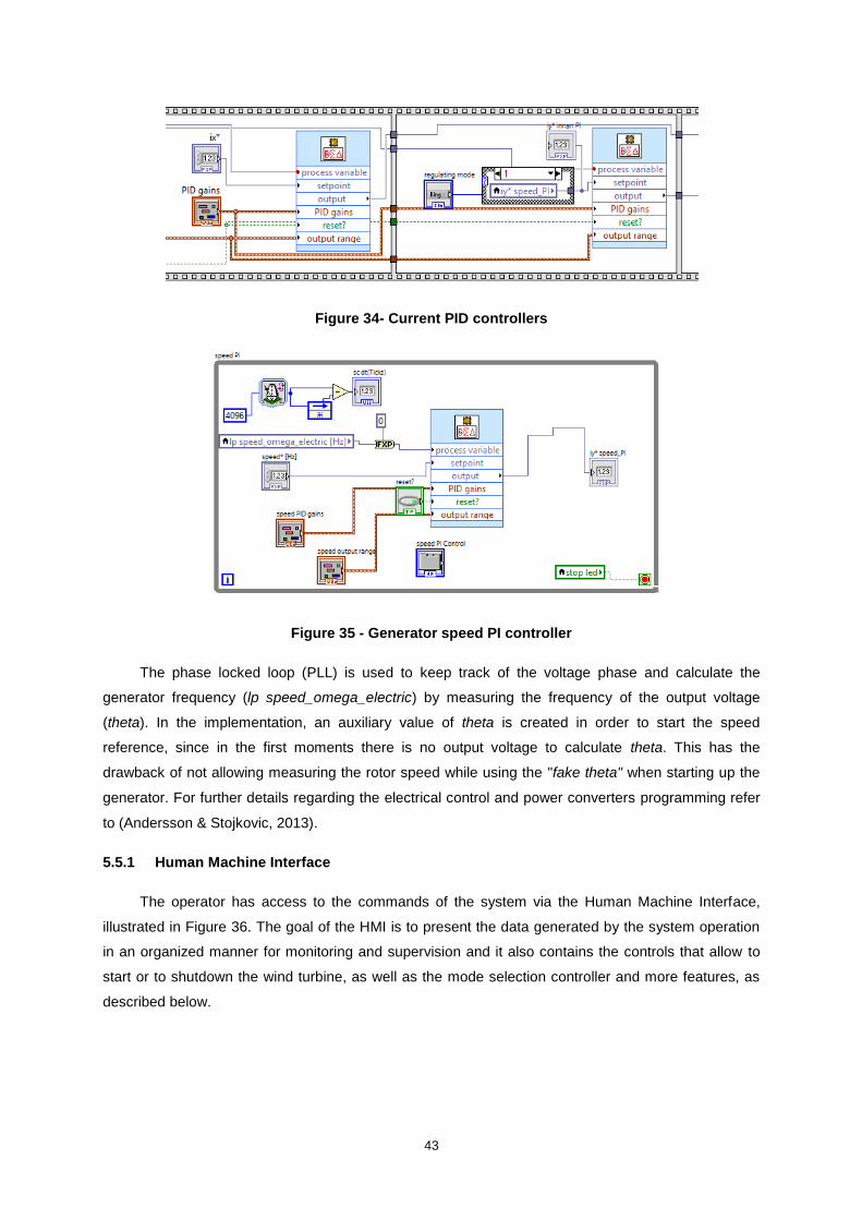
43
Figure 34- Current PID controllers
Figure 35 - Generator speed PI controller
The phase locked loop (PLL) is used to keep track of the voltage phase and calculate the
generator frequency (lp speed_omega_electric) by measuring the frequency of the output voltage
(theta). In the implementation, an auxiliary value of theta is created in order to start the speed
reference, since in the first moments there is no output voltage to calculate theta. This has the
drawback of not allowing measuring the rotor speed while using the "fake theta" when starting up the
generator. For further details regarding the electrical control and power converters programming refer
to (Andersson & Stojkovic, 2013).
5.5.1 Human Machine Interface
The operator has access to the commands of the system via the Human Machine Interface,
illustrated in Figure 36. The goal of the HMI is to present the data generated by the system operation
in an organized manner for monitoring and supervision and it also contains the controls that allow to
start or to shutdown the wind turbine, as well as the mode selection controller and more features, as
described below.
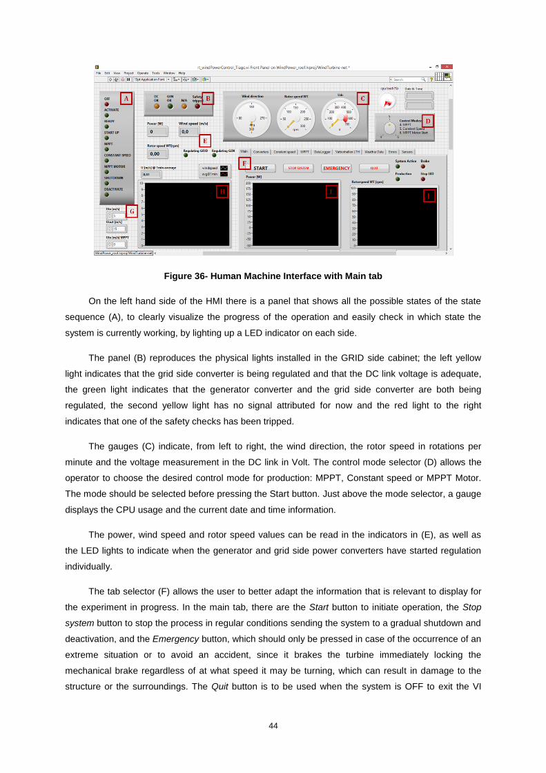
44
Figure 36- Human Machine Interface with Main tab
On the left hand side of the HMI there is a panel that shows all the possible states of the state
sequence (A), to clearly visualize the progress of the operation and easily check in which state the
system is currently working, by lighting up a LED indicator on each side.
The panel (B) reproduces the physical lights installed in the GRID side cabinet; the left yellow
light indicates that the grid side converter is being regulated and that the DC link voltage is adequate,
the green light indicates that the generator converter and the grid side converter are both being
regulated, the second yellow light has no signal attributed for now and the red light to the right
indicates that one of the safety checks has been tripped.
The gauges (C) indicate, from left to right, the wind direction, the rotor speed in rotations per
minute and the voltage measurement in the DC link in Volt. The control mode selector (D) allows the
operator to choose the desired control mode for production: MPPT, Constant speed or MPPT Motor.
The mode should be selected before pressing the Start button. Just above the mode selector, a gauge
displays the CPU usage and the current date and time information.
The power, wind speed and rotor speed values can be read in the indicators in (E), as well as
the LED lights to indicate when the generator and grid side power converters have started regulation
individually.
The tab selector (F) allows the user to better adapt the information that is relevant to display for
the experiment in progress. In the main tab, there are the Start button to initiate operation, the Stop
system button to stop the process in regular conditions sending the system to a gradual shutdown and
deactivation, and the Emergency button, which should only be pressed in case of the occurrence of an
extreme situation or to avoid an accident, since it brakes the turbine immediately locking the
mechanical brake regardless of at what speed it may be turning, which can result in damage to the
structure or the surroundings. The Quit button is to be used when the system is OFF to exit the VI
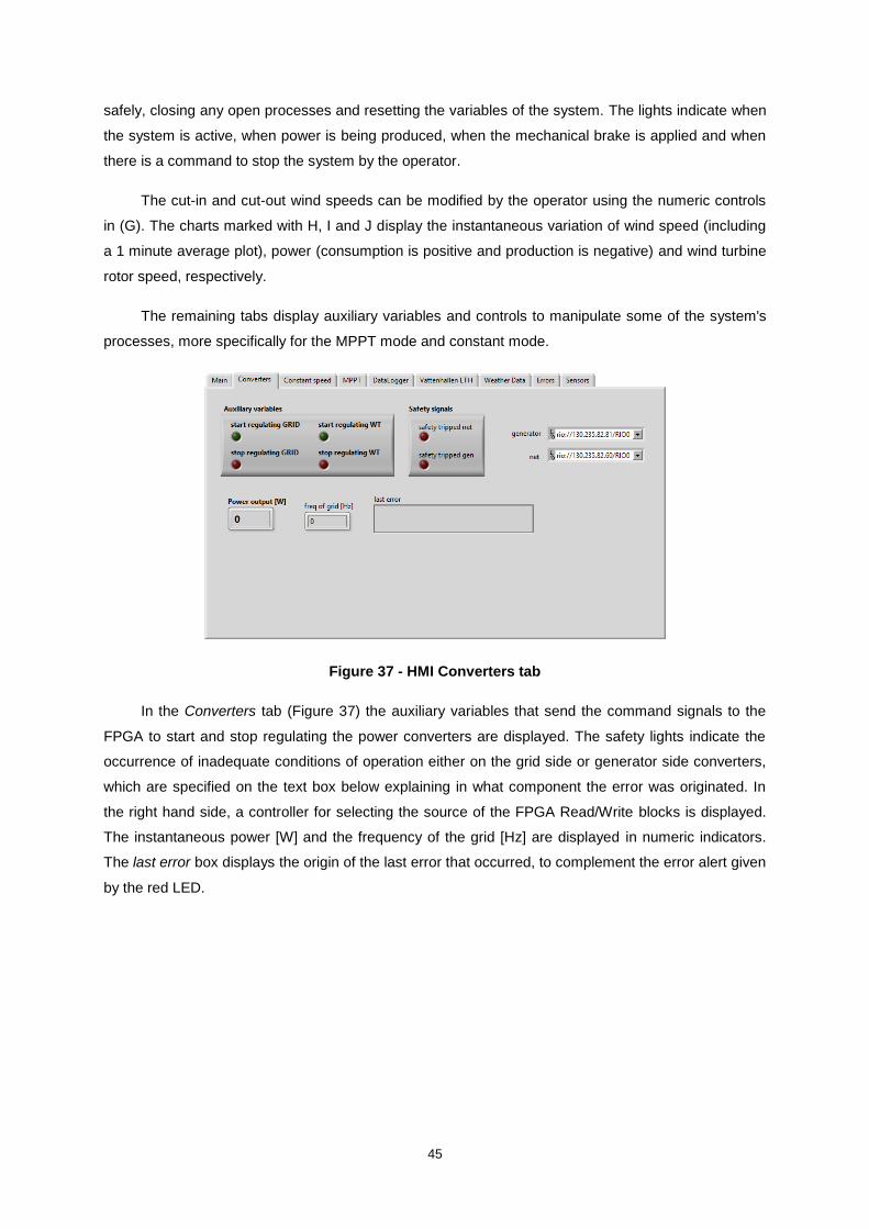
45
safely, closing any open processes and resetting the variables of the system. The lights indicate when
the system is active, when power is being produced, when the mechanical brake is applied and when
there is a command to stop the system by the operator.
The cut-in and cut-out wind speeds can be modified by the operator using the numeric controls
in (G). The charts marked with H, I and J display the instantaneous variation of wind speed (including
a 1 minute average plot), power (consumption is positive and production is negative) and wind turbine
rotor speed, respectively.
The remaining tabs display auxiliary variables and controls to manipulate some of the system's
processes, more specifically for the MPPT mode and constant mode.
Figure 37 - HMI Converters tab
In the Converters tab (Figure 37) the auxiliary variables that send the command signals to the
FPGA to start and stop regulating the power converters are displayed. The safety lights indicate the
occurrence of inadequate conditions of operation either on the grid side or generator side converters,
which are specified on the text box below explaining in what component the error was originated. In
the right hand side, a controller for selecting the source of the FPGA Read/Write blocks is displayed.
The instantaneous power [W] and the frequency of the grid [Hz] are displayed in numeric indicators.
The last error box displays the origin of the last error that occurred, to complement the error alert given
by the red LED.
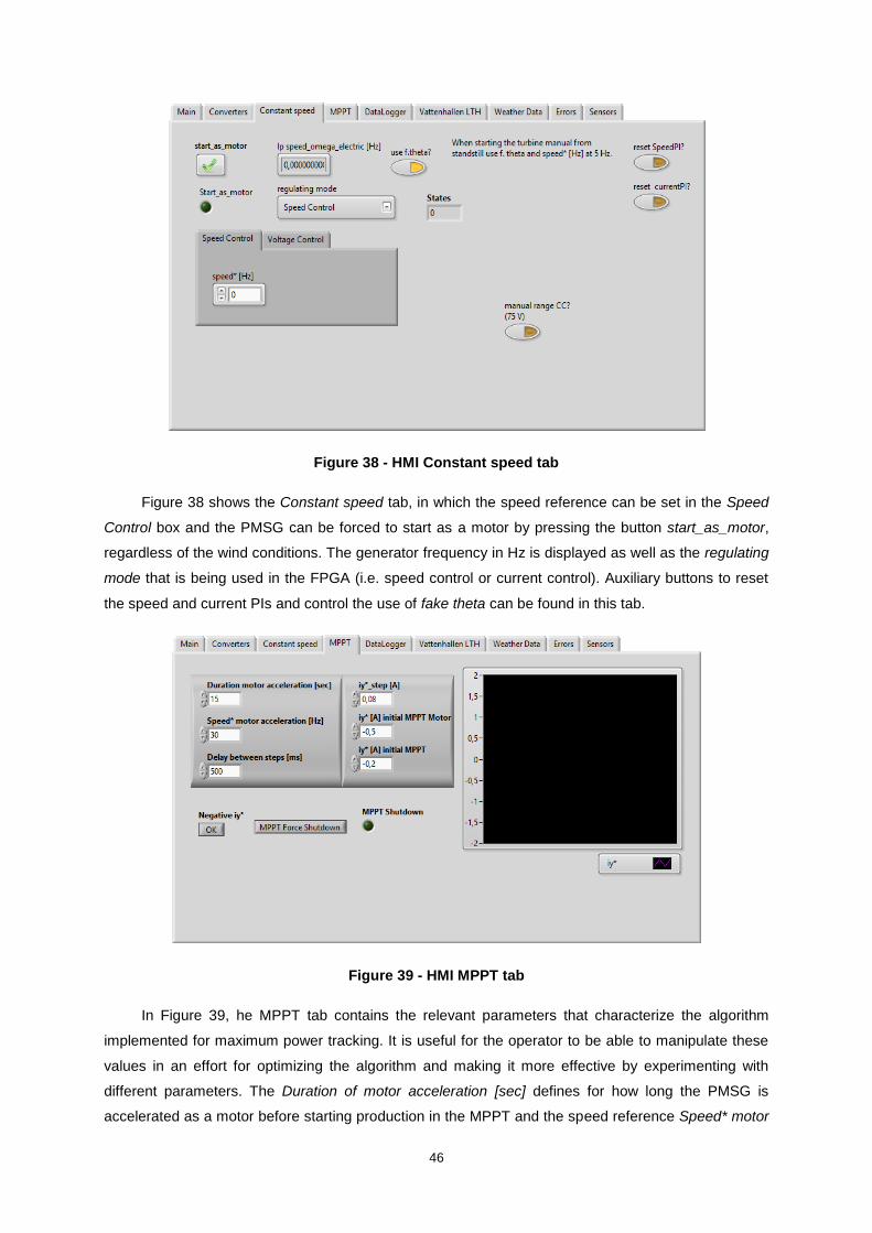
46
Figure 38 - HMI Constant speed tab
Figure 38 shows the Constant speed tab, in which the speed reference can be set in the Speed
Control box and the PMSG can be forced to start as a motor by pressing the button start_as_motor,
regardless of the wind conditions. The generator frequency in Hz is displayed as well as the regulating
mode that is being used in the FPGA (i.e. speed control or current control). Auxiliary buttons to reset
the speed and current PIs and control the use of fake theta can be found in this tab.
Figure 39 - HMI MPPT tab
In Figure 39, he MPPT tab contains the relevant parameters that characterize the algorithm
implemented for maximum power tracking. It is useful for the operator to be able to manipulate these
values in an effort for optimizing the algorithm and making it more effective by experimenting with
different parameters. The Duration of motor acceleration [sec] defines for how long the PMSG is
accelerated as a motor before starting production in the MPPT and the speed reference Speed* motor

47
acceleration stipulates the rotor speed to reach before starting production. The delay between steps is
an important parameter to fine tune, since it defines how long the system waits between applying the
perturbation in rotor speed and observing its impact on the power production. The iy* parameters on
the right define the step in current reference to apply between iterations and the negative current
reference at which the MPPT method is initiated. The variation in current reference iy* is plotted on the
graph to the right to provide a better visualization of the process.
The remaining tabs are provided in the Appendix section since they are less relevant for the
operation of the control system: Datalogger, Vattenhallen LTH, Weather data, Errors and Sensors.
5.5.2 I/O Field Programmable Gate Array
The VI that performs the overall control of the system is installed in the real time controller of the
grid side, as mentioned previously. The command signals to the low level microcontrollers and the
measurements from these are communicated to and from the FPGAs via the Read/Write function in
LabVIEW, as illustrated in Figure 40.
Figure 40 - Read from FPGA
The code on the FPGA of both microcontrollers imposes a series of safety limits to the power
converters. A logic signal is sent from the FPGA in case any of the parameters exceeds the limitations
established (safety tripped), such as:
Grid side Generator side
High current (>20A) High current (>20A)
High voltage (>300V) High voltage (>300V)
High current dq (>20A) High current dq (>20A)
Low voltage (<5V) Low voltage (<5V)
Inverter error (signal from the inverter) Inverter error (signal from the inverter)
High frequency (>1000Hz)
Table 4 - Safety signals from the FPGA
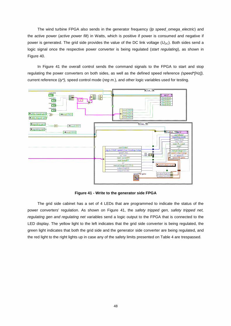
48
The wind turbine FPGA also sends in the generator frequency (lp speed_omega_electric) and
the active power (active power filt) in Watts, which is positive if power is consumed and negative if
power is generated. The grid side provides the value of the DC link voltage (UDC). Both sides send a
logic signal once the respective power converter is being regulated (start regulating), as shown in
Figure 40.
In Figure 41 the overall control sends the command signals to the FPGA to start and stop
regulating the power converters on both sides, as well as the defined speed reference (speed*[Hz]),
current reference (iy*), speed control mode (reg m.), and other logic variables used for testing.
Figure 41 - Write to the generator side FPGA
The grid side cabinet has a set of 4 LEDs that are programmed to indicate the status of the
power converters' regulation. As shown on Figure 41, the safety tripped gen, safety tripped net,
regulating gen and regulating net variables send a logic output to the FPGA that is connected to the
LED display. The yellow light to the left indicates that the grid side converter is being regulated, the
green light indicates that both the grid side and the generator side converter are being regulated, and
the red light to the right lights up in case any of the safety limits presented on Table 4 are trespassed.
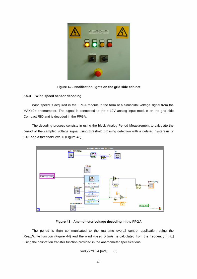
49
Figure 42 - Notification lights on the grid side cabinet
5.5.3 Wind speed sensor decoding
Wind speed is acquired in the FPGA module in the form of a sinusoidal voltage signal from the
MAX40+ anemometer. The signal is connected to the +-10V analog input module on the grid side
Compact RIO and is decoded in the FPGA.
The decoding process consists in using the block Analog Period Measurement to calculate the
period of the sampled voltage signal using threshold crossing detection with a defined hysteresis of
0,01 and a threshold level 0 (Figure 43).
Figure 43 - Anemometer voltage decoding in the FPGA
The period is then communicated to the real-time overall control application using the
Read/Write function (Figure 44) and the wind speed U [m/s] is calculated from the frequency f [Hz]
using the calibration transfer function provided in the anemometer specifications:
U=0,77*f+0,4 [m/s] (5)
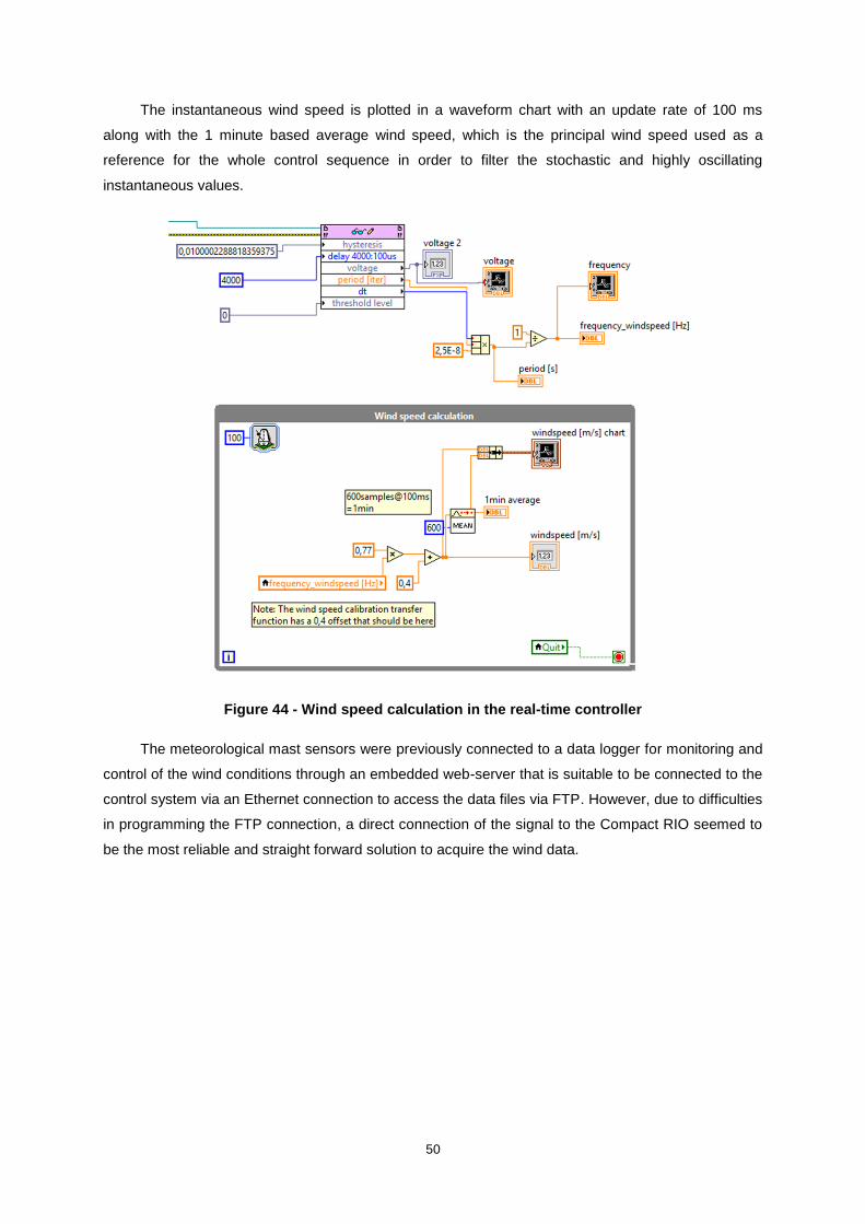
50
The instantaneous wind speed is plotted in a waveform chart with an update rate of 100 ms
along with the 1 minute based average wind speed, which is the principal wind speed used as a
reference for the whole control sequence in order to filter the stochastic and highly oscillating
instantaneous values.
Figure 44 - Wind speed calculation in the real-time controller
The meteorological mast sensors were previously connected to a data logger for monitoring and
control of the wind conditions through an embedded web-server that is suitable to be connected to the
control system via an Ethernet connection to access the data files via FTP. However, due to difficulties
in programming the FTP connection, a direct connection of the signal to the Compact RIO seemed to
be the most reliable and straight forward solution to acquire the wind data.
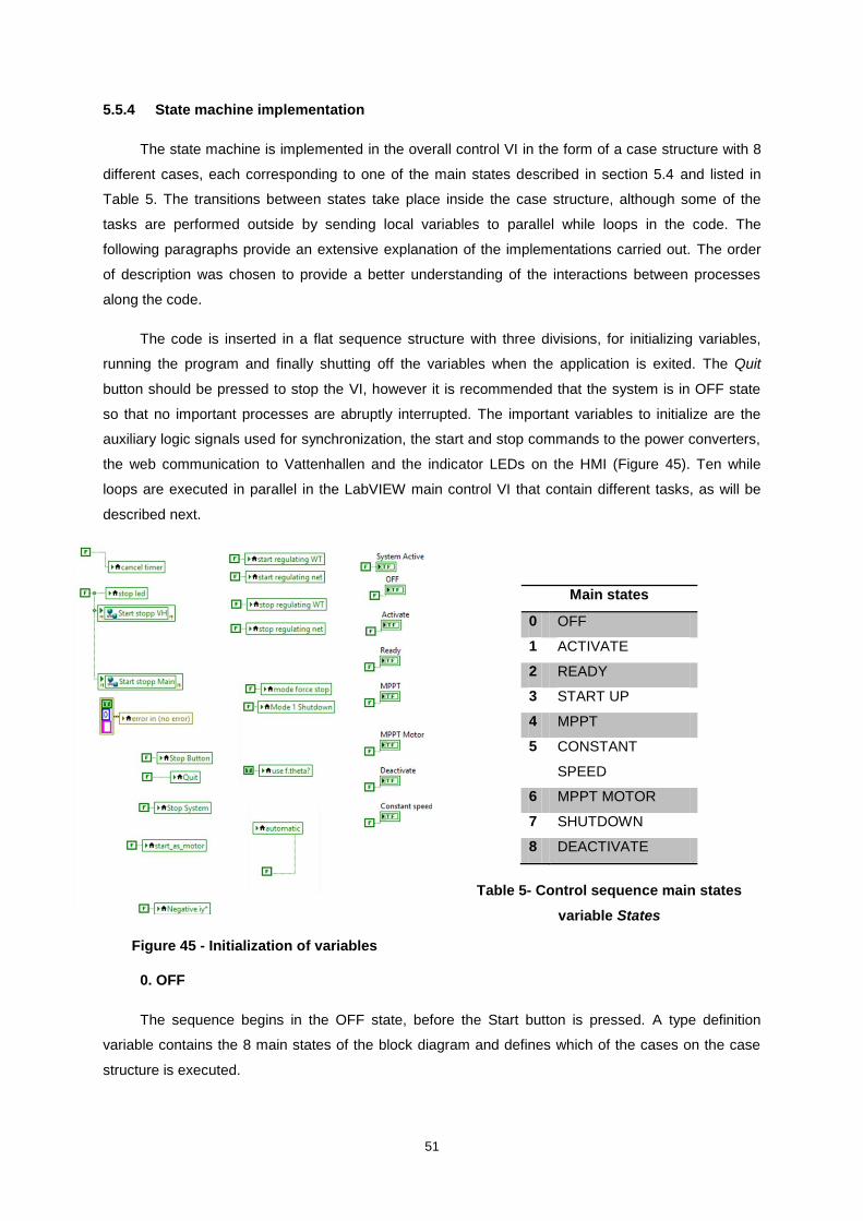
51
5.5.4 State machine implementation
The state machine is implemented in the overall control VI in the form of a case structure with 8
different cases, each corresponding to one of the main states described in section 5.4 and listed in
Table 5. The transitions between states take place inside the case structure, although some of the
tasks are performed outside by sending local variables to parallel while loops in the code. The
following paragraphs provide an extensive explanation of the implementations carried out. The order
of description was chosen to provide a better understanding of the interactions between processes
along the code.
The code is inserted in a flat sequence structure with three divisions, for initializing variables,
running the program and finally shutting off the variables when the application is exited. The Quit
button should be pressed to stop the VI, however it is recommended that the system is in OFF state
so that no important processes are abruptly interrupted. The important variables to initialize are the
auxiliary logic signals used for synchronization, the start and stop commands to the power converters,
the web communication to Vattenhallen and the indicator LEDs on the HMI (Figure 45). Ten while
loops are executed in parallel in the LabVIEW main control VI that contain different tasks, as will be
described next.
Figure 45 - Initialization of variables
Main states
0 OFF
1 ACTIVATE
2 READY
3 START UP
4 MPPT
5 CONSTANT
SPEED
6 MPPT MOTOR
7 SHUTDOWN
8 DEACTIVATE
Table 5- Control sequence main states
variable States
0. OFF
The sequence begins in the OFF state, before the Start button is pressed. A type definition
variable contains the 8 main states of the block diagram and defines which of the cases on the case
structure is executed.
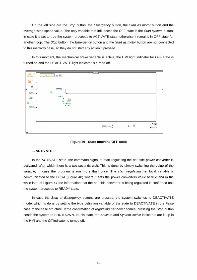
52
On the left side are the Stop button, the Emergency button, the Start as motor button and the
average wind speed value. The only variable that influences the OFF state is the Start system button;
in case it is set to true the system proceeds to ACTIVATE state, otherwise it remains in OFF state for
another loop. The Stop button, the Emergency button and the Start as motor button are not connected
to this inactivity case, so they do not start any action if pressed.
In this moment, the mechanical brake variable is active, the HMI light indicator for OFF state is
turned on and the DEACTIVATE light indicator is turned off.
Figure 46 - State machine OFF state
1. ACTIVATE
In the ACTIVATE state, the command signal to start regulating the net side power converter is
activated, after which there is a two seconds wait. This is done by simply switching the value of the
variable, in case the program is run more than once. The start regulating net local variable is
communicated to the FPGA (Figure 48) where it sets the power converters value to true and in the
while loop of Figure 47 the information that the net side converter is being regulated is confirmed and
the system proceeds to READY state.
In case the Stop or Emergency buttons are pressed, the system switches to DEACTIVATE
mode, which is done by setting the type definition variable of the state to DEACTIVATE in the False
case of the case structure. If the confirmation of regulating net never comes, pressing the Stop button
sends the system to SHUTDOWN. In this state, the Activate and System Active indicators are lit up in
the HMI and the Off indicator is turned off.
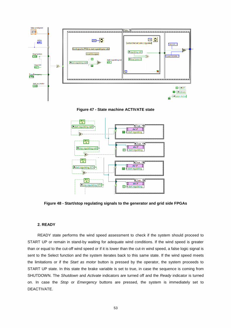
53
Figure 47 - State machine ACTIVATE state
Figure 48 - Start/stop regulating signals to the generator and grid side FPGAs
2. READY
READY state performs the wind speed assessment to check if the system should proceed to
START UP or remain in stand-by waiting for adequate wind conditions. If the wind speed is greater
than or equal to the cut-off wind speed or if it is lower than the cut-in wind speed, a false logic signal is
sent to the Select function and the system iterates back to this same state. If the wind speed meets
the limitations or if the Start as motor button is pressed by the operator, the system proceeds to
START UP state. In this state the brake variable is set to true, in case the sequence is coming from
SHUTDOWN. The Shutdown and Activate indicators are turned off and the Ready indicator is turned
on. In case the Stop or Emergency buttons are pressed, the system is immediately set to
DEACTIVATE.
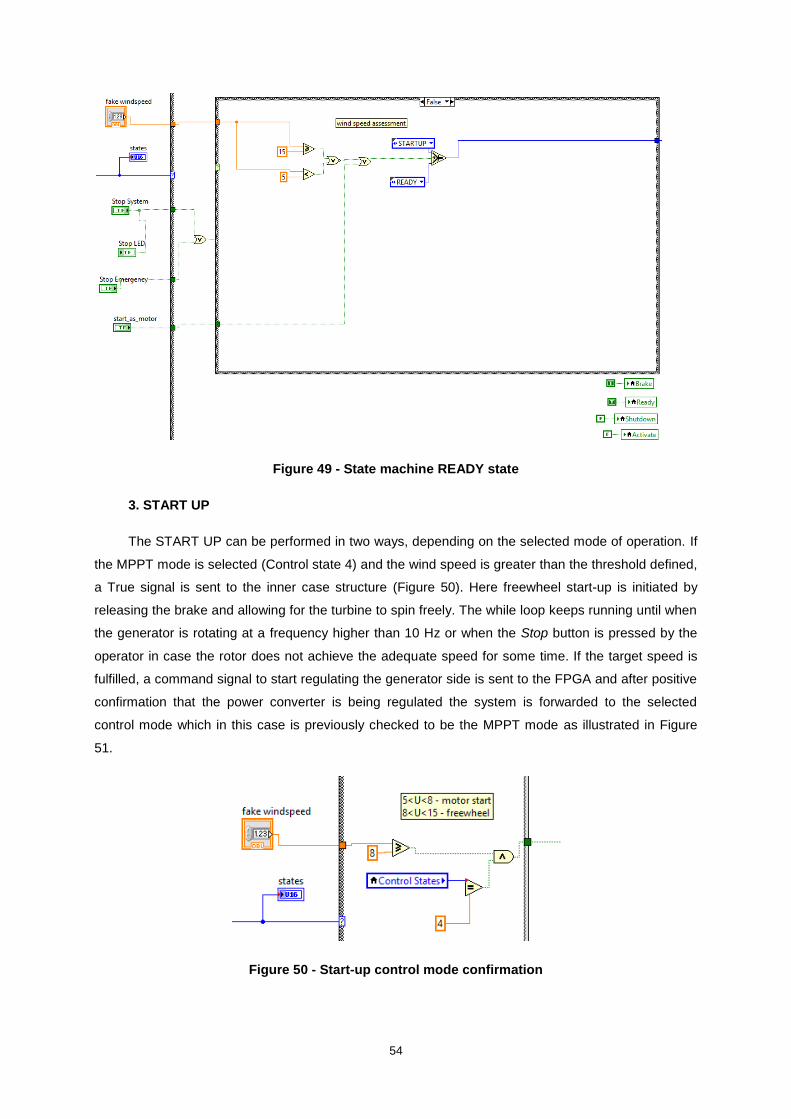
54
Figure 49 - State machine READY state
3. START UP
The START UP can be performed in two ways, depending on the selected mode of operation. If
the MPPT mode is selected (Control state 4) and the wind speed is greater than the threshold defined,
a True signal is sent to the inner case structure (Figure 50). Here freewheel start-up is initiated by
releasing the brake and allowing for the turbine to spin freely. The while loop keeps running until when
the generator is rotating at a frequency higher than 10 Hz or when the Stop button is pressed by the
operator in case the rotor does not achieve the adequate speed for some time. If the target speed is
fulfilled, a command signal to start regulating the generator side is sent to the FPGA and after positive
confirmation that the power converter is being regulated the system is forwarded to the selected
control mode which in this case is previously checked to be the MPPT mode as illustrated in Figure
51.
Figure 50 - Start-up control mode confirmation
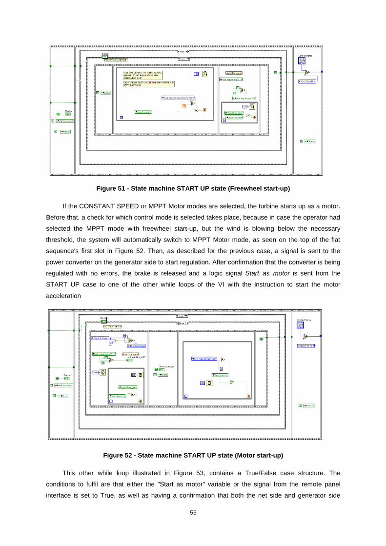
55
Figure 51 - State machine START UP state (Freewheel start-up)
If the CONSTANT SPEED or MPPT Motor modes are selected, the turbine starts up as a motor.
Before that, a check for which control mode is selected takes place, because in case the operator had
selected the MPPT mode with freewheel start-up, but the wind is blowing below the necessary
threshold, the system will automatically switch to MPPT Motor mode, as seen on the top of the flat
sequence's first slot in Figure 52. Then, as described for the previous case, a signal is sent to the
power converter on the generator side to start regulation. After confirmation that the converter is being
regulated with no errors, the brake is released and a logic signal Start_as_motor is sent from the
START UP case to one of the other while loops of the VI with the instruction to start the motor
acceleration
Figure 52 - State machine START UP state (Motor start-up)
This other while loop illustrated in Figure 53, contains a True/False case structure. The
conditions to fulfil are that either the "Start as motor" variable or the signal from the remote panel
interface is set to True, as well as having a confirmation that both the net side and generator side
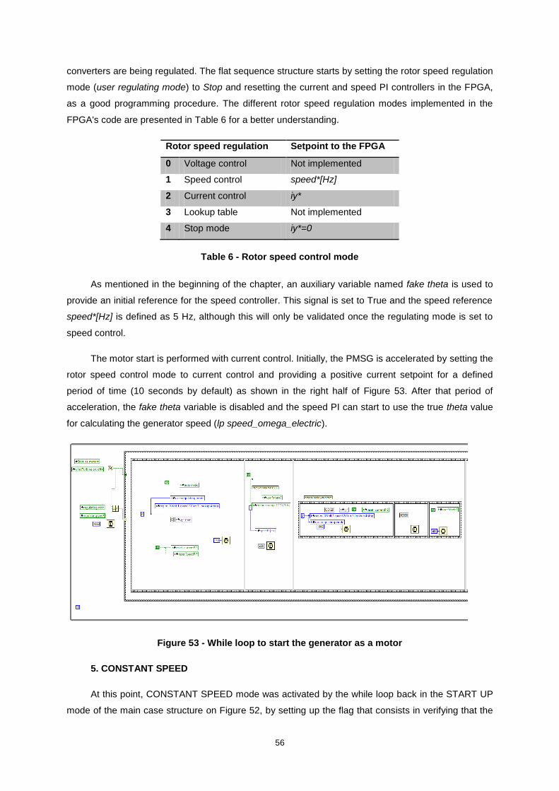
56
converters are being regulated. The flat sequence structure starts by setting the rotor speed regulation
mode (user regulating mode) to Stop and resetting the current and speed PI controllers in the FPGA,
as a good programming procedure. The different rotor speed regulation modes implemented in the
FPGA's code are presented in Table 6 for a better understanding.
Rotor speed regulation Setpoint to the FPGA
0 Voltage control Not implemented
1 Speed control speed*[Hz]
2 Current control iy*
3 Lookup table Not implemented
4 Stop mode iy*=0
Table 6 - Rotor speed control mode
As mentioned in the beginning of the chapter, an auxiliary variable named fake theta is used to
provide an initial reference for the speed controller. This signal is set to True and the speed reference
speed*[Hz] is defined as 5 Hz, although this will only be validated once the regulating mode is set to
speed control.
The motor start is performed with current control. Initially, the PMSG is accelerated by setting the
rotor speed control mode to current control and providing a positive current setpoint for a defined
period of time (10 seconds by default) as shown in the right half of Figure 53. After that period of
acceleration, the fake theta variable is disabled and the speed PI can start to use the true theta value
for calculating the generator speed (lp speed_omega_electric).
Figure 53 - While loop to start the generator as a motor
5. CONSTANT SPEED
At this point, CONSTANT SPEED mode was activated by the while loop back in the START UP
mode of the main case structure on Figure 52, by setting up the flag that consists in verifying that the
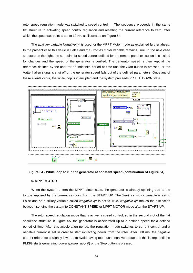
57
rotor speed regulation mode was switched to speed control. The sequence proceeds in the same
flat structure to activating speed control regulation and resetting the current reference to zero, after
which the speed set-point is set to 10 Hz, as illustrated on Figure 54.
The auxiliary variable Negative iy* is used for the MPPT Motor mode as explained further ahead.
In the present case this value is False and the Start as motor variable remains True. In the next case
structure on the right, the set-point for speed control defined for the remote panel execution is checked
for changes and the speed of the generator is verified. The generator speed is then kept at the
reference defined by the user for an indefinite period of time until the Stop button is pressed, or the
Vattenhallen signal is shut off or the generator speed falls out of the defined parameters. Once any of
these events occur, the while loop is interrupted and the system proceeds to SHUTDOWN state.
Figure 54 - While loop to run the generator at constant speed (continuation of Figure 54)
6. MPPT MOTOR
When the system enters the MPPT Motor state, the generator is already spinning due to the
torque imposed by the current set-point from the START UP. The Start_as_motor variable is set to
False and an auxiliary variable called Negative iy* is set to True. Negative iy* makes the distinction
between sending the system to CONSTANT SPEED or MPPT MOTOR mode after the START UP.
The rotor speed regulation mode that is active is speed control, so in the second slot of the flat
sequence structure in Figure 55, the generator is accelerated up to a defined speed for a defined
period of time. After this acceleration period, the regulation mode switches to current control and a
negative current is set in order to start extracting power from the rotor. After 500 ms, the negative
current reference is slightly lowered to avoid having too much negative torque and this is kept until the
PMSG starts generating power (power_avg<0) or the Stop button is pressed.
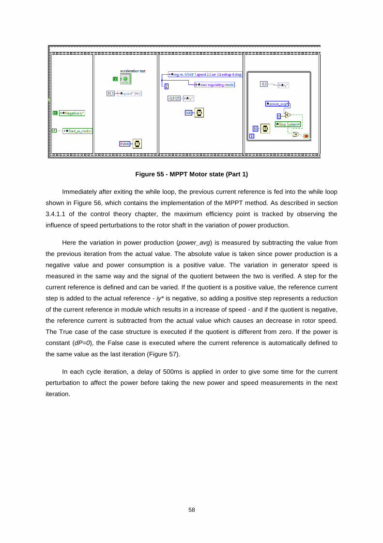
58
Figure 55 - MPPT Motor state (Part 1)
Immediately after exiting the while loop, the previous current reference is fed into the while loop
shown in Figure 56, which contains the implementation of the MPPT method. As described in section
3.4.1.1 of the control theory chapter, the maximum efficiency point is tracked by observing the
influence of speed perturbations to the rotor shaft in the variation of power production.
Here the variation in power production (power_avg) is measured by subtracting the value from
the previous iteration from the actual value. The absolute value is taken since power production is a
negative value and power consumption is a positive value. The variation in generator speed is
measured in the same way and the signal of the quotient between the two is verified. A step for the
current reference is defined and can be varied. If the quotient is a positive value, the reference current
step is added to the actual reference - iy* is negative, so adding a positive step represents a reduction
of the current reference in module which results in a increase of speed - and if the quotient is negative,
the reference current is subtracted from the actual value which causes an decrease in rotor speed.
The True case of the case structure is executed if the quotient is different from zero. If the power is
constant (dP=0), the False case is executed where the current reference is automatically defined to
the same value as the last iteration (Figure 57).
In each cycle iteration, a delay of 500ms is applied in order to give some time for the current
perturbation to affect the power before taking the new power and speed measurements in the next
iteration.
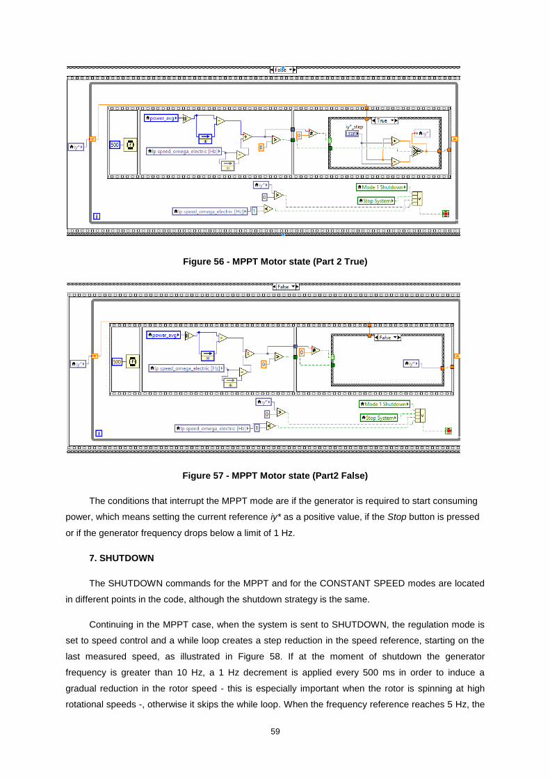
59
Figure 56 - MPPT Motor state (Part 2 True)
Figure 57 - MPPT Motor state (Part2 False)
The conditions that interrupt the MPPT mode are if the generator is required to start consuming
power, which means setting the current reference iy* as a positive value, if the Stop button is pressed
or if the generator frequency drops below a limit of 1 Hz.
7. SHUTDOWN
The SHUTDOWN commands for the MPPT and for the CONSTANT SPEED modes are located
in different points in the code, although the shutdown strategy is the same.
Continuing in the MPPT case, when the system is sent to SHUTDOWN, the regulation mode is
set to speed control and a while loop creates a step reduction in the speed reference, starting on the
last measured speed, as illustrated in Figure 58. If at the moment of shutdown the generator
frequency is greater than 10 Hz, a 1 Hz decrement is applied every 500 ms in order to induce a
gradual reduction in the rotor speed - this is especially important when the rotor is spinning at high
rotational speeds -, otherwise it skips the while loop. When the frequency reference reaches 5 Hz, the
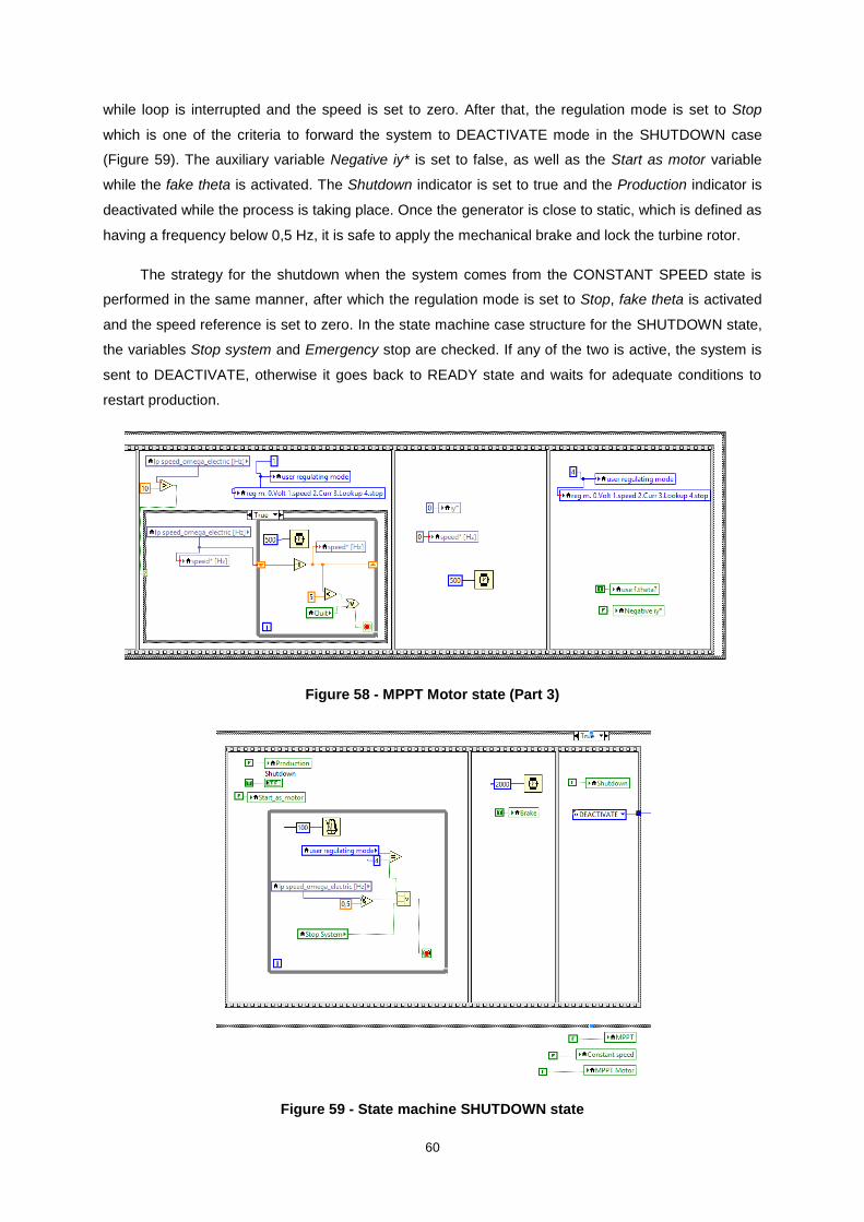
60
while loop is interrupted and the speed is set to zero. After that, the regulation mode is set to Stop
which is one of the criteria to forward the system to DEACTIVATE mode in the SHUTDOWN case
(Figure 59). The auxiliary variable Negative iy* is set to false, as well as the Start as motor variable
while the fake theta is activated. The Shutdown indicator is set to true and the Production indicator is
deactivated while the process is taking place. Once the generator is close to static, which is defined as
having a frequency below 0,5 Hz, it is safe to apply the mechanical brake and lock the turbine rotor.
The strategy for the shutdown when the system comes from the CONSTANT SPEED state is
performed in the same manner, after which the regulation mode is set to Stop, fake theta is activated
and the speed reference is set to zero. In the state machine case structure for the SHUTDOWN state,
the variables Stop system and Emergency stop are checked. If any of the two is active, the system is
sent to DEACTIVATE, otherwise it goes back to READY state and waits for adequate conditions to
restart production.
Figure 58 - MPPT Motor state (Part 3)
Figure 59 - State machine SHUTDOWN state
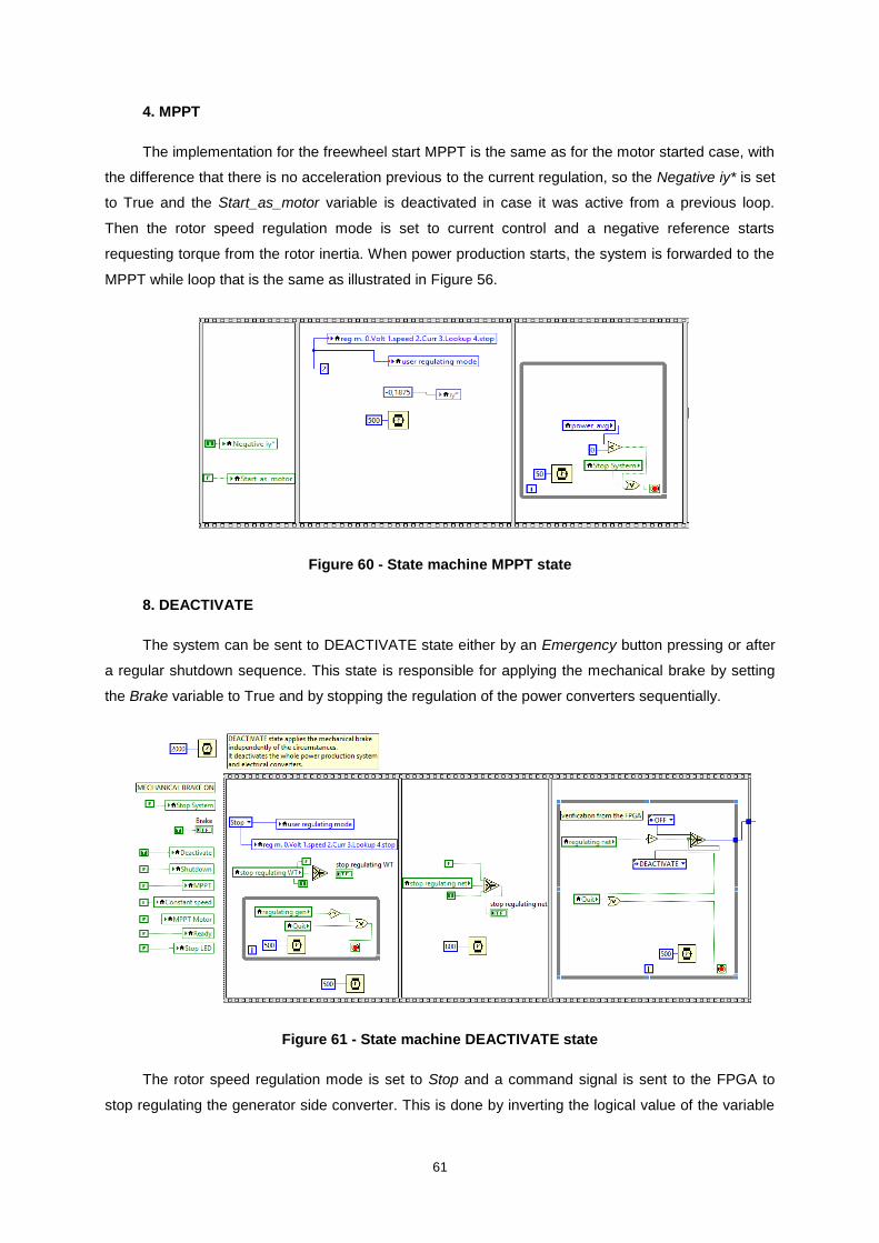
61
4. MPPT
The implementation for the freewheel start MPPT is the same as for the motor started case, with
the difference that there is no acceleration previous to the current regulation, so the Negative iy* is set
to True and the Start_as_motor variable is deactivated in case it was active from a previous loop.
Then the rotor speed regulation mode is set to current control and a negative reference starts
requesting torque from the rotor inertia. When power production starts, the system is forwarded to the
MPPT while loop that is the same as illustrated in Figure 56.
Figure 60 - State machine MPPT state
8. DEACTIVATE
The system can be sent to DEACTIVATE state either by an Emergency button pressing or after
a regular shutdown sequence. This state is responsible for applying the mechanical brake by setting
the Brake variable to True and by stopping the regulation of the power converters sequentially.
Figure 61 - State machine DEACTIVATE state
The rotor speed regulation mode is set to Stop and a command signal is sent to the FPGA to
stop regulating the generator side converter. This is done by inverting the logical value of the variable

62
stop regulating WT. Once the response from the FPGA is received and having the value of the
variable regulating gen set to True, the sequence proceeds to stopping the regulation of the net side
converter in the same way. When confirmation is obtained, the system is directed to OFF state. In this
state, all the indicators from the other state machine cases are deactivated and the indicator
Deactivate is turned on. The system is now back to OFF state waiting for a command to start.
5.5.5 Data logging
Since this is an experimental system, it is important to have a reliable and practical data saving
solution. To save data for condition monitoring and result analysis, the creation of a data logger was
necessary. This was done by creating a Shared Variable called data that stores the following values:
Wind speed average [m/s]
Wind speed [m/s]
Rotor speed reference [rpm]
Power [W]
Rotor speed [rpm]
Brake signal Boolean
Control state 0-8
Current reference [A]
Table 7- Variables saved by the data logger
The values of power and rotor speed are averaged from the 20 latest iterations in order to get a
smoother curve instead of a digital square signal. The generator speed reference speed*[Hz] is
multiplied by a constant of 3,75 to obtain the correspondent value in rotor speed reference in rpm
(Figure 62).
Figure 62 - Data logger while loop
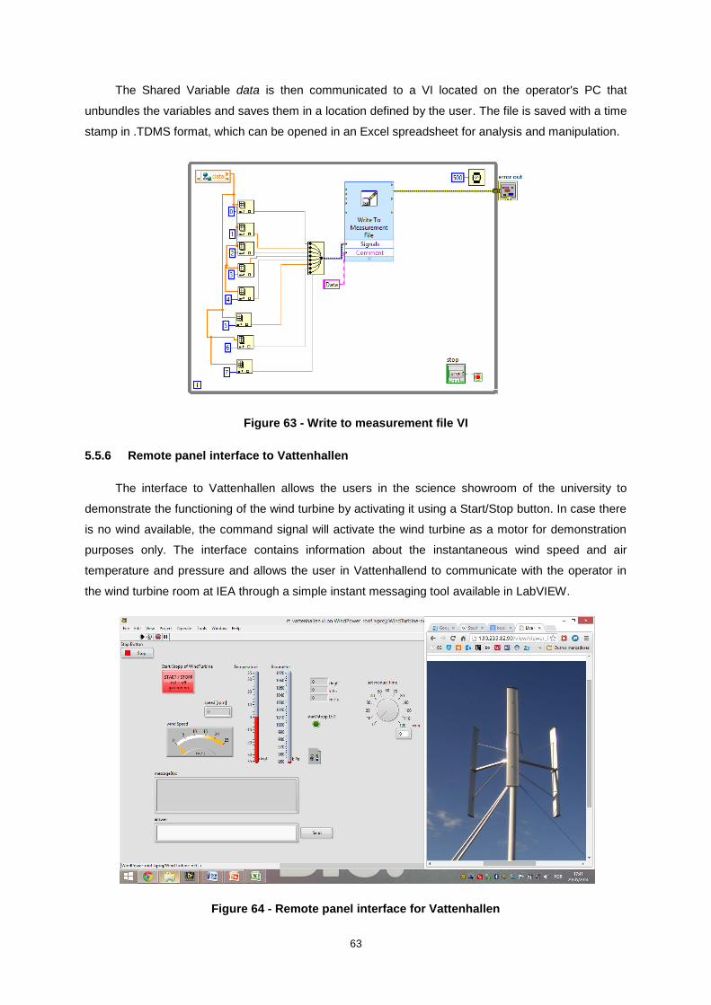
63
The Shared Variable data is then communicated to a VI located on the operator's PC that
unbundles the variables and saves them in a location defined by the user. The file is saved with a time
stamp in .TDMS format, which can be opened in an Excel spreadsheet for analysis and manipulation.
Figure 63 - Write to measurement file VI
5.5.6 Remote panel interface to Vattenhallen
The interface to Vattenhallen allows the users in the science showroom of the university to
demonstrate the functioning of the wind turbine by activating it using a Start/Stop button. In case there
is no wind available, the command signal will activate the wind turbine as a motor for demonstration
purposes only. The interface contains information about the instantaneous wind speed and air
temperature and pressure and allows the user in Vattenhallend to communicate with the operator in
the wind turbine room at IEA through a simple instant messaging tool available in LabVIEW.
Figure 64 - Remote panel interface for Vattenhallen

64
6 Performance tests on the wind turbine
This chapter describes the experimental procedures performed on the system in order to test the
functioning of the features implemented, and also the performance of the wind turbine in operation.
6.1 Communication between the PLCs
Data acquisition and communication are some of the most important factors when designing an
embedded system. A series of tests were performed to ensure that the communication path between
the programmable logic controllers was reliable. The Compact RIOs have a built-in communication
line that ensures transfer of data between the FPGA module and the real time module. As described in
section 5.2, the data transfer between the two microcontrollers is performed via Ethernet connection.
In this experiment, a simple program was developed to test the transfer of data between the net
side real-time module and its FPGA module and also between the generator side real-time module
and the FPGA on the net side Compact RIO, as illustrated in Figure 65.
Figure 65 - Communication tests on the PLCs
The test program consists on sending a variable A from the real-time controller to an FPGA VI
that applies a unitary increment to A and creates a new variable B, which is sent back to the real-time
VI (Figure 66).
Figure 66 - Code of the communication test in the GRID side FPGA VI to apply the increment
As presented in the block diagram of Figure 67, a FPGA VI reference is opened on the real time
VI and in the Read/Write block the value of A is written and the value of B is read from the FPGA. The
control panel shows the variables A and B in two indicators.
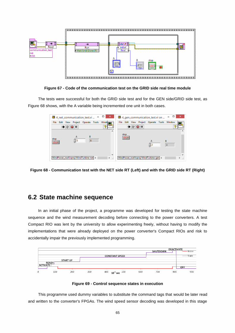
65
Figure 67 - Code of the communication test on the GRID side real time module
The tests were successful for both the GRID side test and for the GEN side/GRID side test, as
Figure 68 shows, with the A variable being incremented one unit in both cases.
Figure 68 - Communication test with the NET side RT (Left) and with the GRID side RT (Right)
6.2 State machine sequence
In an initial phase of the project, a programme was developed for testing the state machine
sequence and the wind measurement decoding before connecting to the power converters. A test
Compact RIO was lent by the university to allow experimenting freely, without having to modify the
implementations that were already deployed on the power converter's Compact RIOs and risk to
accidentally impair the previously implemented programming.
Figure 69 - Control sequence states in execution
This programme used dummy variables to substitute the command tags that would be later read
and written to the converter's FPGAs. The wind speed sensor decoding was developed in this stage
10-1 sec
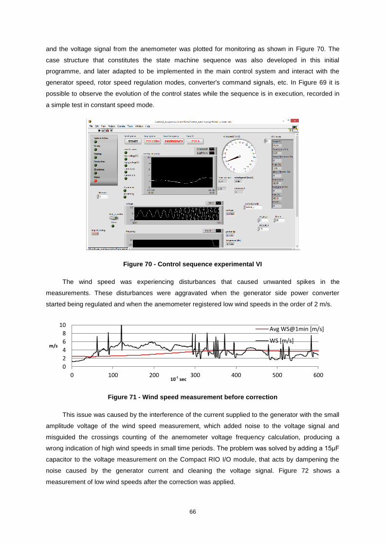
66
and the voltage signal from the anemometer was plotted for monitoring as shown in Figure 70. The
case structure that constitutes the state machine sequence was also developed in this initial
programme, and later adapted to be implemented in the main control system and interact with the
generator speed, rotor speed regulation modes, converter's command signals, etc. In Figure 69 it is
possible to observe the evolution of the control states while the sequence is in execution, recorded in
a simple test in constant speed mode.
Figure 70 - Control sequence experimental VI
The wind speed was experiencing disturbances that caused unwanted spikes in the
measurements. These disturbances were aggravated when the generator side power converter
started being regulated and when the anemometer registered low wind speeds in the order of 2 m/s.
Figure 71 - Wind speed measurement before correction
This issue was caused by the interference of the current supplied to the generator with the small
amplitude voltage of the wind speed measurement, which added noise to the voltage signal and
misguided the crossings counting of the anemometer voltage frequency calculation, producing a
wrong indication of high wind speeds in small time periods. The problem was solved by adding a 15μF
capacitor to the voltage measurement on the Compact RIO I/O module, that acts by dampening the
noise caused by the generator current and cleaning the voltage signal. Figure 72 shows a
measurement of low wind speeds after the correction was applied.
0
2
4
6
8
10
0 100 200 300 400 500 600
Avg WS@1min [m/s]
WS [m/s]
10-1 sec
m/s
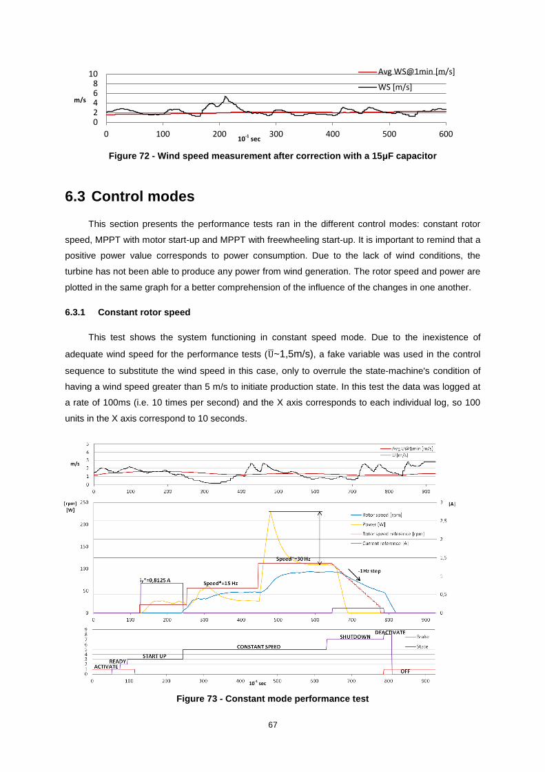
67
Figure 72 - Wind speed measurement after correction with a 15μF capacitor
6.3 Control modes
This section presents the performance tests ran in the different control modes: constant rotor
speed, MPPT with motor start-up and MPPT with freewheeling start-up. It is important to remind that a
positive power value corresponds to power consumption. Due to the lack of wind conditions, the
turbine has not been able to produce any power from wind generation. The rotor speed and power are
plotted in the same graph for a better comprehension of the influence of the changes in one another.
6.3.1 Constant rotor speed
This test shows the system functioning in constant speed mode. Due to the inexistence of
adequate wind speed for the performance tests ( ~1,5m/s), a fake variable was used in the control
sequence to substitute the wind speed in this case, only to overrule the state-machine's condition of
having a wind speed greater than 5 m/s to initiate production state. In this test the data was logged at
a rate of 100ms (i.e. 10 times per second) and the X axis corresponds to each individual log, so 100
units in the X axis correspond to 10 seconds.
Figure 73 - Constant mode performance test
0 2 4 6 8
10
0 100 200 300 400 500 600
Avg WS@1min [m/s]
WS [m/s]
m/s
m/s
10-1 sec
10-1 sec
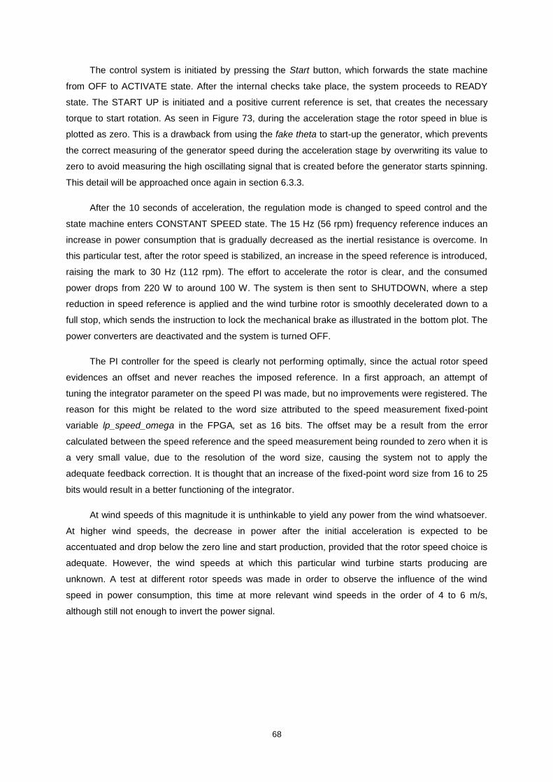
68
The control system is initiated by pressing the Start button, which forwards the state machine
from OFF to ACTIVATE state. After the internal checks take place, the system proceeds to READY
state. The START UP is initiated and a positive current reference is set, that creates the necessary
torque to start rotation. As seen in Figure 73, during the acceleration stage the rotor speed in blue is
plotted as zero. This is a drawback from using the fake theta to start-up the generator, which prevents
the correct measuring of the generator speed during the acceleration stage by overwriting its value to
zero to avoid measuring the high oscillating signal that is created before the generator starts spinning.
This detail will be approached once again in section 6.3.3.
After the 10 seconds of acceleration, the regulation mode is changed to speed control and the
state machine enters CONSTANT SPEED state. The 15 Hz (56 rpm) frequency reference induces an
increase in power consumption that is gradually decreased as the inertial resistance is overcome. In
this particular test, after the rotor speed is stabilized, an increase in the speed reference is introduced,
raising the mark to 30 Hz (112 rpm). The effort to accelerate the rotor is clear, and the consumed
power drops from 220 W to around 100 W. The system is then sent to SHUTDOWN, where a step
reduction in speed reference is applied and the wind turbine rotor is smoothly decelerated down to a
full stop, which sends the instruction to lock the mechanical brake as illustrated in the bottom plot. The
power converters are deactivated and the system is turned OFF.
The PI controller for the speed is clearly not performing optimally, since the actual rotor speed
evidences an offset and never reaches the imposed reference. In a first approach, an attempt of
tuning the integrator parameter on the speed PI was made, but no improvements were registered. The
reason for this might be related to the word size attributed to the speed measurement fixed-point
variable lp_speed_omega in the FPGA, set as 16 bits. The offset may be a result from the error
calculated between the speed reference and the speed measurement being rounded to zero when it is
a very small value, due to the resolution of the word size, causing the system not to apply the
adequate feedback correction. It is thought that an increase of the fixed-point word size from 16 to 25
bits would result in a better functioning of the integrator.
At wind speeds of this magnitude it is unthinkable to yield any power from the wind whatsoever.
At higher wind speeds, the decrease in power after the initial acceleration is expected to be
accentuated and drop below the zero line and start production, provided that the rotor speed choice is
adequate. However, the wind speeds at which this particular wind turbine starts producing are
unknown. A test at different rotor speeds was made in order to observe the influence of the wind
speed in power consumption, this time at more relevant wind speeds in the order of 4 to 6 m/s,
although still not enough to invert the power signal.
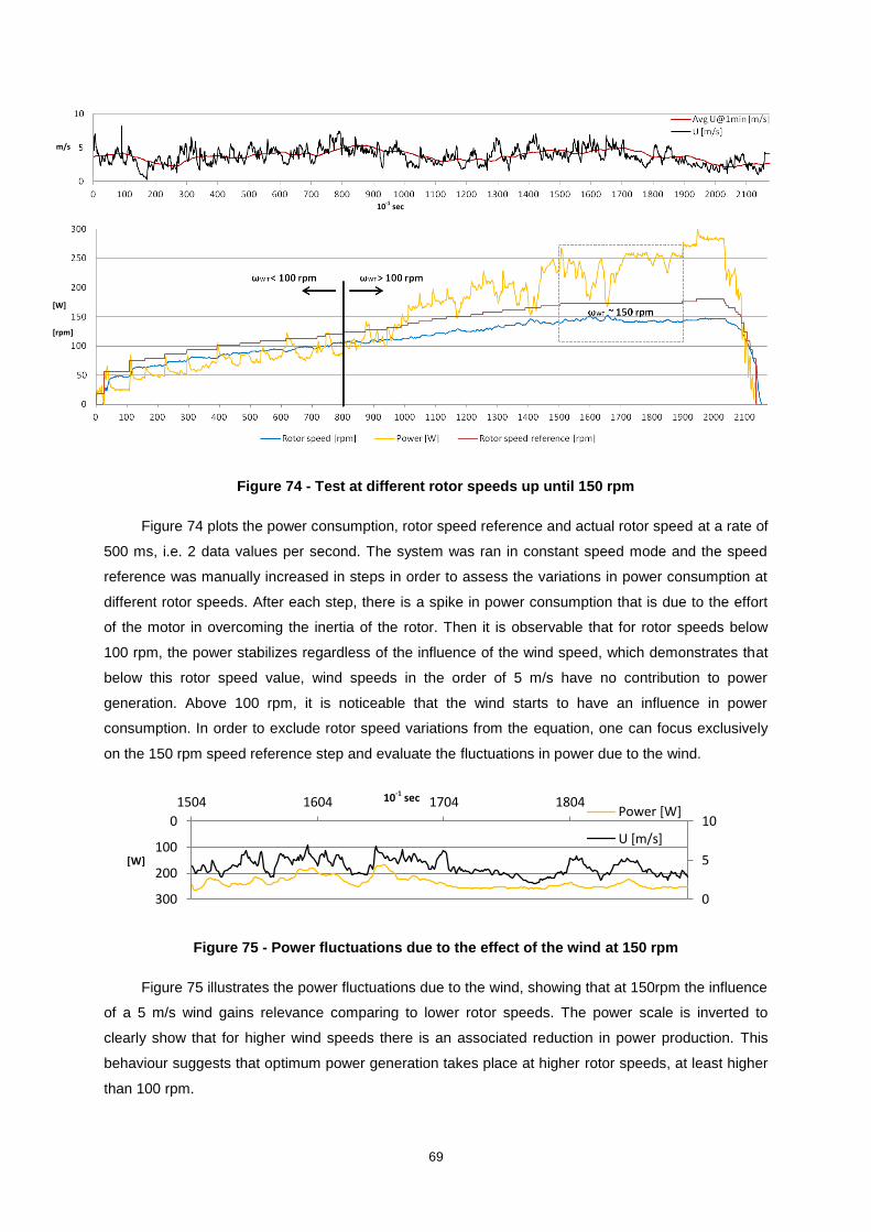
69
Figure 74 - Test at different rotor speeds up until 150 rpm
Figure 74 plots the power consumption, rotor speed reference and actual rotor speed at a rate of
500 ms, i.e. 2 data values per second. The system was ran in constant speed mode and the speed
reference was manually increased in steps in order to assess the variations in power consumption at
different rotor speeds. After each step, there is a spike in power consumption that is due to the effort
of the motor in overcoming the inertia of the rotor. Then it is observable that for rotor speeds below
100 rpm, the power stabilizes regardless of the influence of the wind speed, which demonstrates that
below this rotor speed value, wind speeds in the order of 5 m/s have no contribution to power
generation. Above 100 rpm, it is noticeable that the wind starts to have an influence in power
consumption. In order to exclude rotor speed variations from the equation, one can focus exclusively
on the 150 rpm speed reference step and evaluate the fluctuations in power due to the wind.
Figure 75 - Power fluctuations due to the effect of the wind at 150 rpm
Figure 75 illustrates the power fluctuations due to the wind, showing that at 150rpm the influence
of a 5 m/s wind gains relevance comparing to lower rotor speeds. The power scale is inverted to
clearly show that for higher wind speeds there is an associated reduction in power production. This
behaviour suggests that optimum power generation takes place at higher rotor speeds, at least higher
than 100 rpm.
0
5
10 0
100
200
300
1504 1604 1704 1804 Power [W]
U [m/s]
m/s
[W]
[rpm]
10-1 sec
10-1 sec
[W]
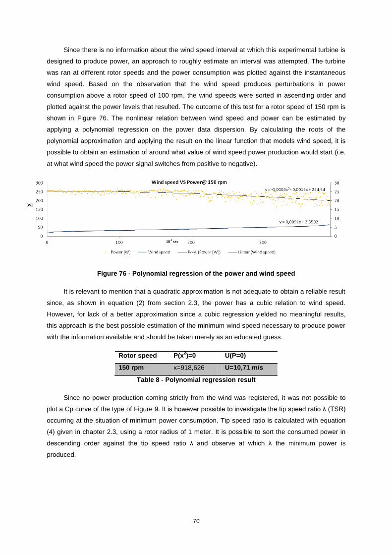
70
Since there is no information about the wind speed interval at which this experimental turbine is
designed to produce power, an approach to roughly estimate an interval was attempted. The turbine
was ran at different rotor speeds and the power consumption was plotted against the instantaneous
wind speed. Based on the observation that the wind speed produces perturbations in power
consumption above a rotor speed of 100 rpm, the wind speeds were sorted in ascending order and
plotted against the power levels that resulted. The outcome of this test for a rotor speed of 150 rpm is
shown in Figure 76. The nonlinear relation between wind speed and power can be estimated by
applying a polynomial regression on the power data dispersion. By calculating the roots of the
polynomial approximation and applying the result on the linear function that models wind speed, it is
possible to obtain an estimation of around what value of wind speed power production would start (i.e.
at what wind speed the power signal switches from positive to negative).
Figure 76 - Polynomial regression of the power and wind speed
It is relevant to mention that a quadratic approximation is not adequate to obtain a reliable result
since, as shown in equation (2) from section 2.3, the power has a cubic relation to wind speed.
However, for lack of a better approximation since a cubic regression yielded no meaningful results,
this approach is the best possible estimation of the minimum wind speed necessary to produce power
with the information available and should be taken merely as an educated guess.
Rotor speed P(x2)=0 U(P=0)
150 rpm x=918,626 U=10,71 m/s
Table 8 - Polynomial regression result
Since no power production coming strictly from the wind was registered, it was not possible to
plot a Cp curve of the type of Figure 9. It is however possible to investigate the tip speed ratio λ (TSR)
occurring at the situation of minimum power consumption. Tip speed ratio is calculated with equation
(4) given in chapter 2.3, using a rotor radius of 1 meter. It is possible to sort the consumed power in
descending order against the tip speed ratio λ and observe at which λ the minimum power is
produced.
[W]
10-1 sec
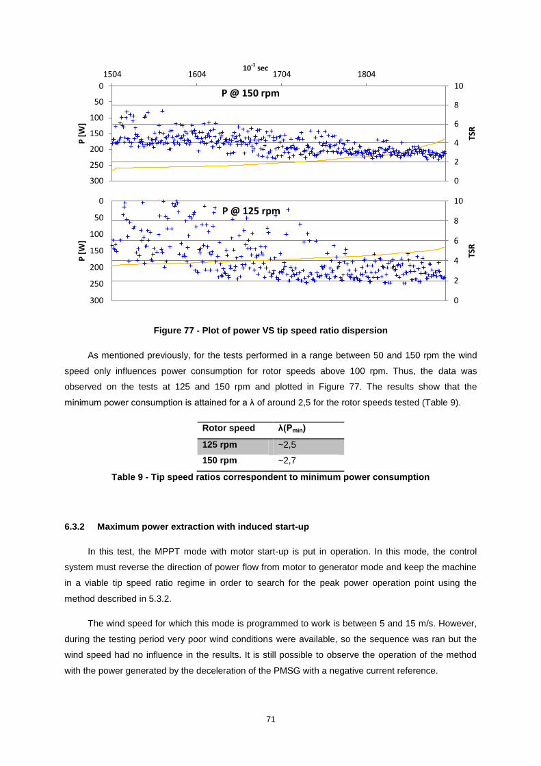
71
Figure 77 - Plot of power VS tip speed ratio dispersion
As mentioned previously, for the tests performed in a range between 50 and 150 rpm the wind
speed only influences power consumption for rotor speeds above 100 rpm. Thus, the data was
observed on the tests at 125 and 150 rpm and plotted in Figure 77. The results show that the
minimum power consumption is attained for a λ of around 2,5 for the rotor speeds tested (Table 9).
Rotor speed λ(Pmin)
125 rpm ~2,5
150 rpm ~2,7
Table 9 - Tip speed ratios correspondent to minimum power consumption
6.3.2 Maximum power extraction with induced start-up
In this test, the MPPT mode with motor start-up is put in operation. In this mode, the control
system must reverse the direction of power flow from motor to generator mode and keep the machine
in a viable tip speed ratio regime in order to search for the peak power operation point using the
method described in 5.3.2.
The wind speed for which this mode is programmed to work is between 5 and 15 m/s. However,
during the testing period very poor wind conditions were available, so the sequence was ran but the
wind speed had no influence in the results. It is still possible to observe the operation of the method
with the power generated by the deceleration of the PMSG with a negative current reference.
0
2
4
6
8
10 0
50
100
150
200
250
300
1504 1604 1704 1804
TSR
P [
W]
P @ 150 rpm
0
2
4
6
8
10 0
50
100
150
200
250
300
TSR
P [
W]
P @ 125 rpm
10-1
sec
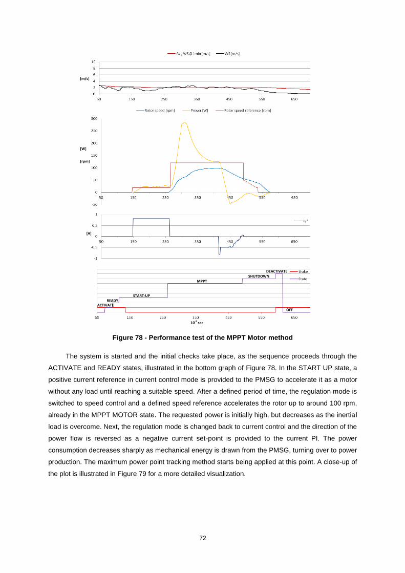
72
Figure 78 - Performance test of the MPPT Motor method
The system is started and the initial checks take place, as the sequence proceeds through the
ACTIVATE and READY states, illustrated in the bottom graph of Figure 78. In the START UP state, a
positive current reference in current control mode is provided to the PMSG to accelerate it as a motor
without any load until reaching a suitable speed. After a defined period of time, the regulation mode is
switched to speed control and a defined speed reference accelerates the rotor up to around 100 rpm,
already in the MPPT MOTOR state. The requested power is initially high, but decreases as the inertial
load is overcome. Next, the regulation mode is changed back to current control and the direction of the
power flow is reversed as a negative current set-point is provided to the current PI. The power
consumption decreases sharply as mechanical energy is drawn from the PMSG, turning over to power
production. The maximum power point tracking method starts being applied at this point. A close-up of
the plot is illustrated in Figure 79 for a more detailed visualization.
10-1 sec
[A]
[W]
[rpm]
[m/s]
ACTIVATE
START-UP
MPPT
START-
SHUTDOWN DEACTIVATE
OFF
READY
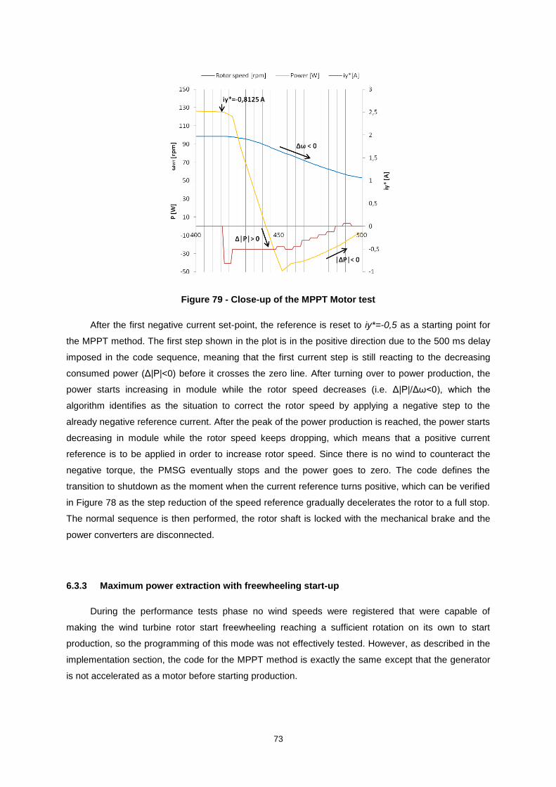
73
Figure 79 - Close-up of the MPPT Motor test
After the first negative current set-point, the reference is reset to iy*=-0,5 as a starting point for
the MPPT method. The first step shown in the plot is in the positive direction due to the 500 ms delay
imposed in the code sequence, meaning that the first current step is still reacting to the decreasing
consumed power (Δ|P|<0) before it crosses the zero line. After turning over to power production, the
power starts increasing in module while the rotor speed decreases (i.e. Δ|P|/Δω<0), which the
algorithm identifies as the situation to correct the rotor speed by applying a negative step to the
already negative reference current. After the peak of the power production is reached, the power starts
decreasing in module while the rotor speed keeps dropping, which means that a positive current
reference is to be applied in order to increase rotor speed. Since there is no wind to counteract the
negative torque, the PMSG eventually stops and the power goes to zero. The code defines the
transition to shutdown as the moment when the current reference turns positive, which can be verified
in Figure 78 as the step reduction of the speed reference gradually decelerates the rotor to a full stop.
The normal sequence is then performed, the rotor shaft is locked with the mechanical brake and the
power converters are disconnected.
6.3.3 Maximum power extraction with freewheeling start-up
During the performance tests phase no wind speeds were registered that were capable of
making the wind turbine rotor start freewheeling reaching a sufficient rotation on its own to start
production, so the programming of this mode was not effectively tested. However, as described in the
implementation section, the code for the MPPT method is exactly the same except that the generator
is not accelerated as a motor before starting production.
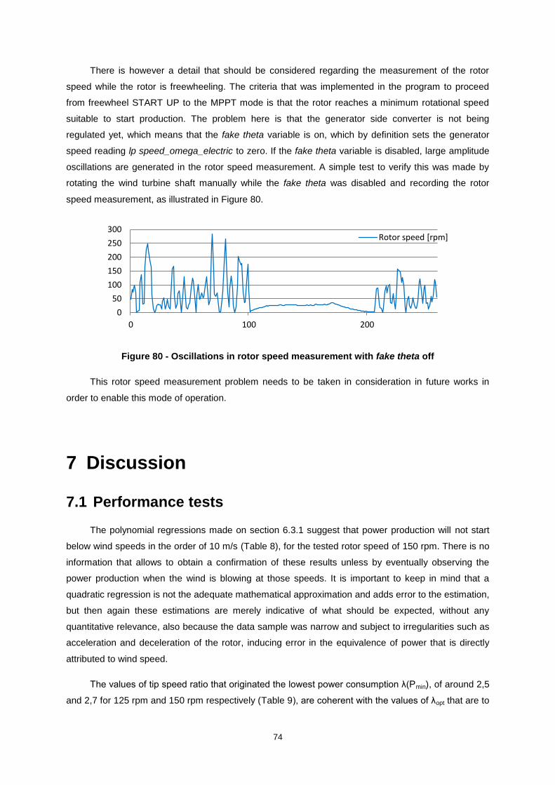
74
There is however a detail that should be considered regarding the measurement of the rotor
speed while the rotor is freewheeling. The criteria that was implemented in the program to proceed
from freewheel START UP to the MPPT mode is that the rotor reaches a minimum rotational speed
suitable to start production. The problem here is that the generator side converter is not being
regulated yet, which means that the fake theta variable is on, which by definition sets the generator
speed reading lp speed_omega_electric to zero. If the fake theta variable is disabled, large amplitude
oscillations are generated in the rotor speed measurement. A simple test to verify this was made by
rotating the wind turbine shaft manually while the fake theta was disabled and recording the rotor
speed measurement, as illustrated in Figure 80.
Figure 80 - Oscillations in rotor speed measurement with fake theta off
This rotor speed measurement problem needs to be taken in consideration in future works in
order to enable this mode of operation.
7 Discussion
7.1 Performance tests
The polynomial regressions made on section 6.3.1 suggest that power production will not start
below wind speeds in the order of 10 m/s (Table 8), for the tested rotor speed of 150 rpm. There is no
information that allows to obtain a confirmation of these results unless by eventually observing the
power production when the wind is blowing at those speeds. It is important to keep in mind that a
quadratic regression is not the adequate mathematical approximation and adds error to the estimation,
but then again these estimations are merely indicative of what should be expected, without any
quantitative relevance, also because the data sample was narrow and subject to irregularities such as
acceleration and deceleration of the rotor, inducing error in the equivalence of power that is directly
attributed to wind speed.
The values of tip speed ratio that originated the lowest power consumption λ(Pmin), of around 2,5
and 2,7 for 125 rpm and 150 rpm respectively (Table 9), are coherent with the values of λopt that are to
0
50
100
150
200
250
300
0 100 200
Rotor speed [rpm]
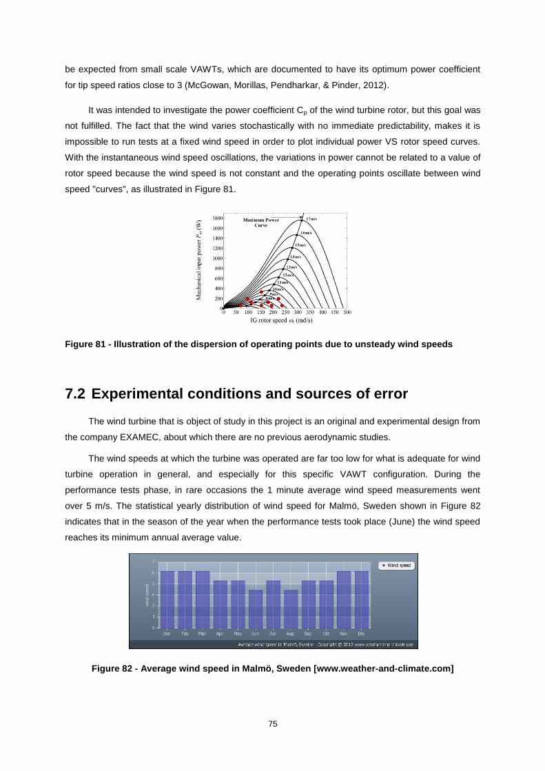
75
be expected from small scale VAWTs, which are documented to have its optimum power coefficient
for tip speed ratios close to 3 (McGowan, Morillas, Pendharkar, & Pinder, 2012).
It was intended to investigate the power coefficient Cp of the wind turbine rotor, but this goal was
not fulfilled. The fact that the wind varies stochastically with no immediate predictability, makes it is
impossible to run tests at a fixed wind speed in order to plot individual power VS rotor speed curves.
With the instantaneous wind speed oscillations, the variations in power cannot be related to a value of
rotor speed because the wind speed is not constant and the operating points oscillate between wind
speed "curves", as illustrated in Figure 81.
Figure 81 - Illustration of the dispersion of operating points due to unsteady wind speeds
7.2 Experimental conditions and sources of error
The wind turbine that is object of study in this project is an original and experimental design from
the company EXAMEC, about which there are no previous aerodynamic studies.
The wind speeds at which the turbine was operated are far too low for what is adequate for wind
turbine operation in general, and especially for this specific VAWT configuration. During the
performance tests phase, in rare occasions the 1 minute average wind speed measurements went
over 5 m/s. The statistical yearly distribution of wind speed for Malmö, Sweden shown in Figure 82
indicates that in the season of the year when the performance tests took place (June) the wind speed
reaches its minimum annual average value.
Figure 82 - Average wind speed in Malmö, Sweden [www.weather-and-climate.com]
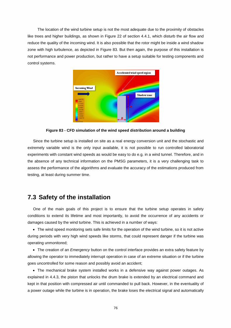
76
The location of the wind turbine setup is not the most adequate due to the proximity of obstacles
like trees and higher buildings, as shown in Figure 22 of section 4.4.1, which disturb the air flow and
reduce the quality of the incoming wind. It is also possible that the rotor might be inside a wind shadow
zone with high turbulence, as depicted in Figure 83. But then again, the purpose of this installation is
not performance and power production, but rather to have a setup suitable for testing components and
control systems.
Figure 83 - CFD simulation of the wind speed distribution around a building
Since the turbine setup is installed on site as a real energy conversion unit and the stochastic and
extremely variable wind is the only input available, it is not possible to run controlled laboratorial
experiments with constant wind speeds as would be easy to do e.g. in a wind tunnel. Therefore, and in
the absence of any technical information on the PMSG parameters, it is a very challenging task to
assess the performance of the algorithms and evaluate the accuracy of the estimations produced from
testing, at least during summer time.
7.3 Safety of the installation
One of the main goals of this project is to ensure that the turbine setup operates in safety
conditions to extend its lifetime and most importantly, to avoid the occurrence of any accidents or
damages caused by the wind turbine. This is achieved in a number of ways:
The wind speed monitoring sets safe limits for the operation of the wind turbine, so it is not active
during periods with very high wind speeds like storms, that could represent danger if the turbine was
operating unmonitored;
The creation of an Emergency button on the control interface provides an extra safety feature by
allowing the operator to immediately interrupt operation in case of an extreme situation or if the turbine
goes uncontrolled for some reason and possibly avoid an accident;
The mechanical brake system installed works in a defensive way against power outages. As
explained in 4.4.3, the piston that unlocks the drum brake is extended by an electrical command and
kept in that position with compressed air until commanded to pull back. However, in the eventuality of
a power outage while the turbine is in operation, the brake loses the electrical signal and automatically

77
returns to the braking position thus protecting the rotor from freewheeling unloaded which in case of
very high speeds could take it up to structurally hazardous speeds;
The meteorological mast is directly connected to the Compact RIO which, due to its exposed
location on the roof, could lead to material damage in case of a lightning strike. The cable with the
wind speed measurement to the Compact RIO is going through a resistance that obstructs the
transmission of very high currents but causes no effect on the low amplitude voltage signal from the
anemometer.
7.4 Evaluation of the success of the project
The development of the automatic operation strategy and the implementation of the control
system were successful. The wind power plant control sequence is implemented and fully operational,
acquiring the wind speed measurement to the monitoring system with accurate values and no
disturbances. The mechanical brake is installed and tested and Vattenhallen's remote panel
connection is up and running.
The programming was a long and iterative process, with situations of the kind "one step forward,
two steps backward". The HMI was designed with the aim of providing a flexible experimental tool and
highly customizable environment to allow the operator to change the parameters that rule the speed
control modes and experiment in order to optimize and fine tune the methods that are implemented.
The implementation of the monitoring and control system was not affected by the lack of wind
conditions, but the performance tests on the speed control modes were impaired by the absence of
adequate wind speeds.
Anyhow, the algorithm for optimal wind energy yield seems to behave according to the theory
that supports it, although no relevant conclusions about its effectiveness can be taken from the testing
results. It is recommended that further experimentation should be made at higher wind speeds in order
to assess the method's real performance.
The main advantage of the Hill Climb Search method is that it does not require prior knowledge
of maximum power at different wind velocities nor electrical machine parameters. In this case, none of
these are known. It was intended to investigate the Cp of the rotor and plot a power curve but the wind
conditions were not favourable during the performance testing, as explained in 7.2.
Owing to the poor wind conditions or to the aerodynamic design of the wind turbine or to a
combination of both, no power was produced from the wind during the testing performed on this
project. It is recommended to perform further studies on the experimental setup, both to confirm the
estimations that resulted from this study and to fine tune and improve the implementations and the
installation.
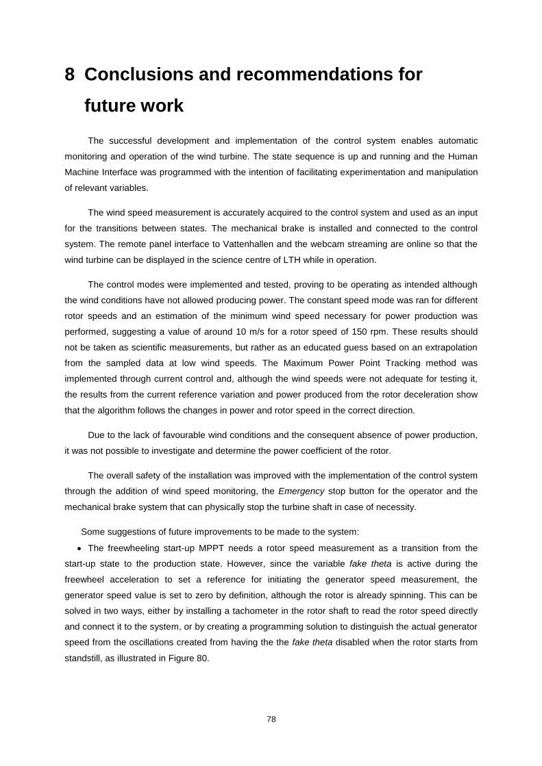
78
8 Conclusions and recommendations for
future work
The successful development and implementation of the control system enables automatic
monitoring and operation of the wind turbine. The state sequence is up and running and the Human
Machine Interface was programmed with the intention of facilitating experimentation and manipulation
of relevant variables.
The wind speed measurement is accurately acquired to the control system and used as an input
for the transitions between states. The mechanical brake is installed and connected to the control
system. The remote panel interface to Vattenhallen and the webcam streaming are online so that the
wind turbine can be displayed in the science centre of LTH while in operation.
The control modes were implemented and tested, proving to be operating as intended although
the wind conditions have not allowed producing power. The constant speed mode was ran for different
rotor speeds and an estimation of the minimum wind speed necessary for power production was
performed, suggesting a value of around 10 m/s for a rotor speed of 150 rpm. These results should
not be taken as scientific measurements, but rather as an educated guess based on an extrapolation
from the sampled data at low wind speeds. The Maximum Power Point Tracking method was
implemented through current control and, although the wind speeds were not adequate for testing it,
the results from the current reference variation and power produced from the rotor deceleration show
that the algorithm follows the changes in power and rotor speed in the correct direction.
Due to the lack of favourable wind conditions and the consequent absence of power production,
it was not possible to investigate and determine the power coefficient of the rotor.
The overall safety of the installation was improved with the implementation of the control system
through the addition of wind speed monitoring, the Emergency stop button for the operator and the
mechanical brake system that can physically stop the turbine shaft in case of necessity.
Some suggestions of future improvements to be made to the system:
The freewheeling start-up MPPT needs a rotor speed measurement as a transition from the
start-up state to the production state. However, since the variable fake theta is active during the
freewheel acceleration to set a reference for initiating the generator speed measurement, the
generator speed value is set to zero by definition, although the rotor is already spinning. This can be
solved in two ways, either by installing a tachometer in the rotor shaft to read the rotor speed directly
and connect it to the system, or by creating a programming solution to distinguish the actual generator
speed from the oscillations created from having the the fake theta disabled when the rotor starts from
standstill, as illustrated in Figure 80.
79
A suggestion to improve the effectiveness of the MPPT method is to make the current reference
step variable, so that larger steps are taken when the operating point is further away from maximum
extraction and smaller steps when it is reaching the peak of the curve. This implementation expected
to cause the algorithm to reach the maximum power point faster with the larger steps and to stay
closer to peak efficiency, by taking smaller steps around the maximum point.
It is observable that the rotor speed reference is being tracked with an offset. The offset may be
a result from the error calculated between the speed reference and the speed measurement in the
speed PI controller being rounded to zero when it is a very small value, due to the resolution of the
word size, causing the system not to apply the adequate feedback correction. It is thought that an
increase of the fixed-point word size of the error variable from 16 to 25 bits would result in a better
functioning of the integrator. A reduction on the sampling rate of the PID might also improve the speed
reference tracking.
If the turbine is to be operated at rotor speeds much higher than 150 rpm it is advisable that
structural improvements are made to the turbine tower and fixings. Vibration and shaking were
observed in the tower supports at rotor speeds above 120 rpm. It is important to gain knowledge about
the structure's limitations to avoid reaching velocities that could lead to turbine damage or, even
worse, to accidents or injuries to people passing by. It would be useful to install a vibration sensor in
the turbine tower to monitor the oscillations and maximize the safety of the installation.
It would be important to test the control modes at higher wind speeds, so testing the wind turbine
during the winter, when average wind speeds are higher, might evidence a better performance on
power production.
9 References
Andersson, M., & Stojkovic, A. (2013). Documentation for the wind power lab turbine - System
overview. Lund, Sweden.
Arrillaga, J. (1998). High Voltage Direct Current Transmission, 2nd Edition. Institution of Electrical
Engineers.
Barakati, S. M., Kazerani, M., & Aplevich, J. D. (2009). Maximum Power Tracking Control for a Wind
Turbine System Including a Matrix Converter. IEEE Transactions on Energy Conversion.
Boyer, S. A. (2010). SCADA Supervisory Control and Data Acquisition ISBN 978-1-936007-09-7.
USA: ISA - International Society of Automation.
Dvorak, P. (4 de June de 2013). Keep the control hardware but make the algorithms easy to change.
Obtido de Windpower Engineering & Development:
http://www.windpowerengineering.com/design/electrical/controls/keep-the-control-hardware-but-make-
the-algorithms-easy-to-change/
Dvorak, P. (5 de February de 2014). Windpower Engineering & Development. Obtido de
http://www.windpowerengineering.com/design/electrical/national-instruments-sites-7-technology-
trends-2014-can-accelerate-productivity/

80
Dvorak, P. (21 de April de 2014). Windpower Engineering & Development. Obtido de How wind farm
monitoring leads to maximum output:
http://www.windpowerengineering.com/design/electrical/controls/wind-farm-monitoring-leads-
maximum-output/
Eldrige, F. R. (1980). Wind Machines, 2nd Edition. New York: Van Nostrand Reinhold.
EU, E. C. (March de 2007). The 2020 climate and energy package. Obtido de
http://ec.europa.eu/clima/policies/package/index_en.htm
Fitzgerald, A. E., Jr., C. K., & Umans, S. (2003). Electrical Machinery, 6th Edition. McGraw-Hill
Companies, Inc.
IEA, I. E. (2013). Key World Energy Statistics. Paris: www.iea.org.
IEA, I. E. (2013). Technology Roadmap Wind Energy. www.iea.com.
Manwell, J. F. (2009). Wind Energy Explained. John Wiley & Sons.
McGowan, R., Morillas, K., Pendharkar, A., & Pinder, M. (2012). Optimization of a Vertical Axis Micro
Wind Turbine for Low Tip Speed Ratio Operation (p.2). Atlanta, USA: The Daniel Guggenheim School
of Aerospace Engineering, Georgia Institute of Technology.
NI, N. I. (2013). Developer's Guide. Obtido de NI LabVIEW for CompactRIO.
NI, N. I. (2014). NI Compact RIO Specifications. Obtido de National Instruments:
http://www.ni.com/compactrio/
Örs, M. (2009). Maximum Power Point Tracking for Small Scale Wind Turbine With Self-Excited
Induction Generator. Cluj-Napoca, Romania: Technical University of Cluj-Napoca, Department of
Automatic Control.
Petitfils, V. (2011). Master Thesis: Setup and performance test of a small-scale vertical axis wind
turbine. Lund, Sweden: Division of Industrial Electrical Engineering and Automation, LTH, Lund
University.
Rohatgi, J. S., & Nelson, V. (1994). Wind Characteristics: An Analysis for the Generation of Wind
Power. Canyon, Texas: Alternative Energy Institute.
Sharpley, N. (21 de April de 2014). How wind farm monitoring leads to maximum output. Windpower
Engineering & Development .
Svensson, J. (2006). Active Distributed Power Systems. Lund, Sweden: Department of Industrial
Engineering and Automation, Lund University.
Tempel, J. v. (2006). Design of Support Structures for Offshore Wind Turbines. PhD Thesis. Delft, NL:
TU Delft.
Thongam, J. S., & Ouhrouche, M. (2011). MPPT Control Methods in Wind Energy Conversion
Systems, Fundamental and Advanced Topics in Wind Power, ISBN:978-953-307-508-2. InTech.
Wang, Q. (2004). An Intelligent maximum Power Extraction Algorithm for Inverter-Based Variable
Speed Wind Turbine Systems. IEEE.
Wind Basics. (2014). Wind Power Engineering & Development Handbook , p. 91.
Zinger, D., & Muljadi, E. (1997). Annualized wind energy improvement using variable speeds. IEEE.
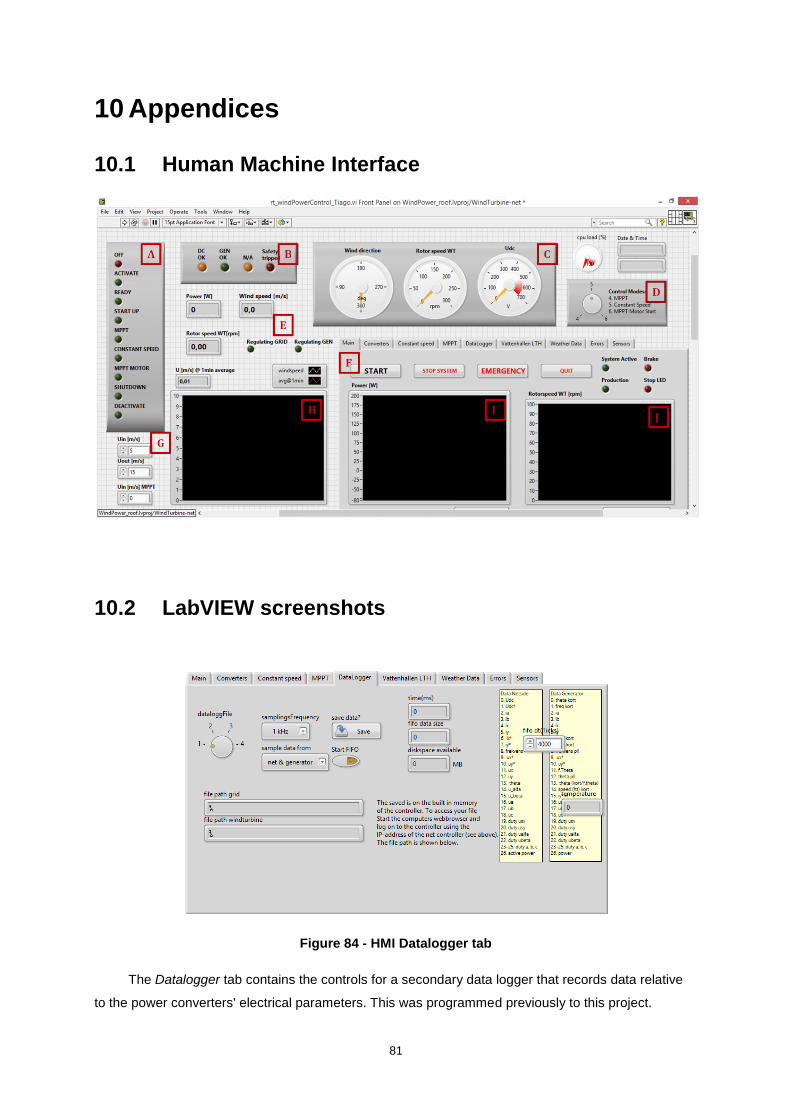
81
10 Appendices
10.1 Human Machine Interface
10.2 LabVIEW screenshots
Figure 84 - HMI Datalogger tab
The Datalogger tab contains the controls for a secondary data logger that records data relative
to the power converters' electrical parameters. This was programmed previously to this project.
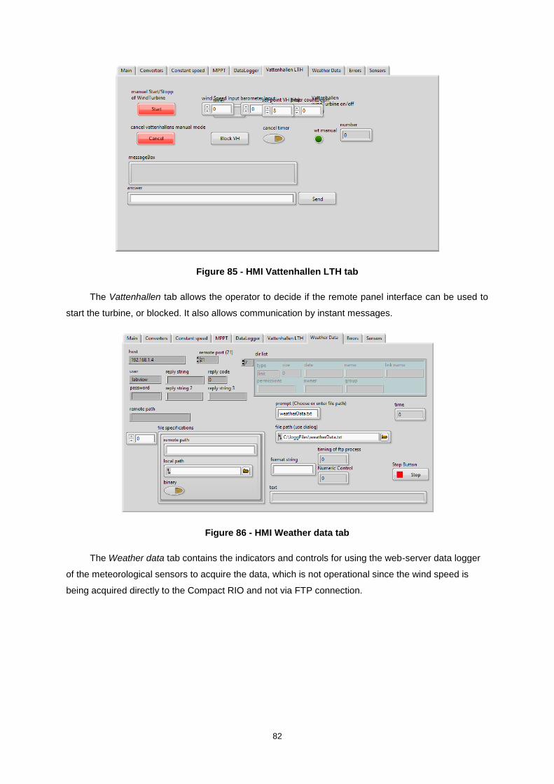
82
Figure 85 - HMI Vattenhallen LTH tab
The Vattenhallen tab allows the operator to decide if the remote panel interface can be used to
start the turbine, or blocked. It also allows communication by instant messages.
Figure 86 - HMI Weather data tab
The Weather data tab contains the indicators and controls for using the web-server data logger
of the meteorological sensors to acquire the data, which is not operational since the wind speed is
being acquired directly to the Compact RIO and not via FTP connection.

83
Figure 87 - HMI Errors tab
The Errors tab displays the status of the several error indicators throughout the code in order to
identify the origin of possible programming mistakes or unusual situations.
Figure 88 - HMI Sensors tab
The Sensors tab displays the electrical signal coming from the wind speed measurement that is
used for decoding, as well as indicators for the air temperature and pressure that are not being
acquired to the control system yet.