Turbulence in vertical axis wind turbine canopiesMatthias Kinzel, Daniel B. Araya, and John O. Dabiri Citation: Physics of Fluids 27, 115102 (2015); doi: 10.1063/1.4935111 View online: http://dx.doi.org/10.1063/1.4935111 View Table of Contents: http://scitation.aip.org/content/aip/journal/pof2/27/11?ver=pdfcov Published by the AIP Publishing Articles you may be interested in On the statistics of wind turbine wake meandering: An experimental investigation Phys. Fluids 27, 075103 (2015); 10.1063/1.4923334 Design of a hydroformed metal blade for vertical-axis wind turbines J. Renewable Sustainable Energy 7, 043135 (2015); 10.1063/1.4928949 Unsteady vortex lattice method coupled with a linear aeroelastic model for horizontal axis windturbine J. Renewable Sustainable Energy 6, 042006 (2014); 10.1063/1.4890830 Analysis of aerodynamic field and noise of a small wind turbine AIP Conf. Proc. 1493, 699 (2012); 10.1063/1.4765563 Power performance of canted blades for a vertical axis wind turbine J. Renewable Sustainable Energy 3, 013106 (2011); 10.1063/1.3549153

This article is copyrighted as indicated in the article. Reuse of AIP content is subject to the terms at: http://scitation.aip.org/termsconditions. Downloaded

to IP: 131.215.70.231 On: Mon, 16 Nov 2015 16:12:43

PHYSICS OF FLUIDS 27, 115102 (2015)

Turbulence in vertical axis wind turbine canopiesMatthias Kinzel,1 Daniel B. Araya,1 and John O. Dabiri1,2,a)1Graduate Aerospace Laboratories, California Institute of Technology,Pasadena, California 91125, USA2Bioengineering, California Institute of Technology, Pasadena, California 91125, USA

(Received 10 February 2015; accepted 20 October 2015; published online 9 November 2015)

Experimental results from three different full scale arrays of vertical-axis wind tur-bines (VAWTs) under natural wind conditions are presented. The wind velocitiesthroughout the turbine arrays are measured using a portable meteorological towerwith seven, vertically staggered, three-component ultrasonic anemometers. The po-wer output of each turbine is recorded simultaneously. The comparison between thehorizontal and vertical energy transport for the different turbine array sizes shows theimportance of vertical transport for large array configurations. Quadrant-hole analysisis employed to gain a better understanding of the vertical energy transport at the topof the VAWT arrays. The results show a striking similarity between the flows in theVAWT arrays and the adjustment region of canopies. Namely, an increase in ejectionsand sweeps and decrease in inward and outward interactions occur inside the turbinearray. Ejections are the strongest contributor, which is in agreement with the literatureon evolving and sparse canopy flows. The influence of the turbine array size on thepower output of the downstream turbines is examined by comparing a streamwise rowof four single turbines with square arrays of nine turbine pairs. The results suggestthat a new boundary layer forms on top of the larger turbine arrays as the flow adjuststo the new roughness length. This increases the turbulent energy transport over thewhole planform area of the turbine array. By contrast, for the four single turbines, thevertical energy transport due to turbulent fluctuations is only increased in the near wakeof the turbines. These findings add to the knowledge of energy transport in turbinearrays and therefore the optimization of the turbine spacing in wind farms. C 2015 AIPPublishing LLC. [http://dx.doi.org/10.1063/1.4935111]

I. INTRODUCTION

A. Energy production in large wind turbine arrays

With wind farms increasing in size, the focus in research is shifting from the efficiency ofsingle wind turbines to the overall performance of the turbine array (see, e.g., Refs. 1 and 2). Thework can be divided into two categories: wind turbine wakes, wake interaction and influence onthe downwind turbines (e.g., Refs. 3, 5, and 6) and the energy transfer between the turbine arrayand the surrounding atmospheric surface layer flow (see Refs. 7–10).

Due to the large dimensions of both the turbine arrays as well as the turbines themselves, fewexperiments have been done in the field (e.g., Refs. 5, 11, and 12), whereas most of the abovementioned studies were conducted in wind tunnel experiments and numerically. The laboratory exper-iments have the limitation that it is challenging to match the high Reynolds number and the turbineblade tip speed ratio simultaneously in a wind tunnel without motorizing the wind turbines. The highReynolds number of the flow and the wind farm dimensions on the order of kilometers also limit thenumerical work to mainly wall modeled large eddy simulations (LES) (see, e.g., Ref. 10).

a)Electronic address: jodabiri@stanford.edu. Current address: School of Engineering, Stanford University, Stanford, Califor-nia 94305, USA.

1070-6631/2015/27(11)/115102/17/$30.00 27, 115102-1 ©2015 AIP Publishing LLC

This article is copyrighted as indicated in the article. Reuse of AIP content is subject to the terms at: http://scitation.aip.org/termsconditions. Downloaded

to IP: 131.215.70.231 On: Mon, 16 Nov 2015 16:12:43

115102-2 Kinzel, Araya, and Dabiri Phys. Fluids 27, 115102 (2015)

The velocity in the wake of a horizontal axis wind turbine (HAWT) takes on the order of 20rotor diameters to recover to the upstream value (see, e.g., Ref. 13). Therefore, a typical turbinespacing of 10 rotor diameters decreases the power output of the downstream turbine by as much as40% (see Ref. 14). Meyers and Meneveau2 recommended an optimal turbine spacing of 16-18 rotordiameters from an economical point of view.

Some studies have investigated algorithms that limit the power output of individual turbinesin order to optimize the overall power output and grid performance by the turbine array (see,e.g., Refs. 15–17). Most studies, however, analyze the energy transport within the turbine arraywith the aim to optimize the turbine spacing. In this context, Cal et al.7 derived equations for thekinetic energy transport from the Reynolds-averaged Navier-Stokes equation for the streamwisedirection,

⟨u⟩ ∂12 ⟨u⟩2

∂x+ ⟨w⟩ ∂

12 ⟨u⟩2

∂z= − 1

ρ⟨u⟩ dp∞

dx− ∂

∂z

(u′w ′ ⟨u⟩ + u′′w ′′ ⟨u⟩)

+u′w ′ ∂ ⟨u⟩

∂z+u′′w ′′

∂ ⟨u⟩∂z− P(z). (1)

In the equation above, primes indicate turbulent fluctuations, over bars temporal averaging, andangle brackets spatial averaging in the horizontal plane. u and w are the streamwise and verticalvelocities along the x and z directions. The dispersive stress,

u′′w ′′

, is caused by the correla-

tion between spatially non-homegeneous horizontal and vertical mean velocities. It is defined asu′′ = u − ⟨u⟩ and w ′′ = w − ⟨w⟩. Cal et al.7 show that this term is small compared to the Reynoldsstresses,

u′w ′, which is why it will not be considered in the following analysis of the planform

momentum flux. P(z) results from the product of the spatially averaged velocity, ⟨u⟩, and the aver-aged thrust force,

f x. The viscous terms are neglected because of the high Reynolds number of

the flow (Re ≈ 106). The Coriolis force term can also be neglected due to the Rossby number beingRo = U

f L≫ 1, where U ≈ 10 m s−1 is the characteristic velocity, f = 2Ωsinϕ ≈ 10−4 rad/s is the

Coriolis frequency, and L = 40 m the maximum characteristic length scale of the turbine arrays.From the kinetic energy equation (Equation (1)), it can be seen that there are two ways that

energy enters a turbine array: horizontally from the sides and vertically from above. The corre-sponding terms are

Ps

=

12ρAs⟨u⟩3 (2)

for the streamwise transport by the mean flow andPp

= −ρAp ⟨u⟩

u′w ′

(3)

for the vertical energy transport by the turbulent stresses as well asPt

=

12ρAt⟨u⟩3, (4)

for the transverse energy transport. As, Ap, and At denote the projected area of the turbine arrayin the streamwise, planform, and transverse direction, respectively. The planform energy transport,Pp, is defined negative such that positive values correspond to a momentum flux into the turbinearray.

Once the energy from the horizontal flux has been converted into power by the turbines in theupstream rows or dissipated by viscous stresses the planform momentum flux becomes the mainsource of energy (see, e.g., Ref. 7). Therefore, the vertical energy transport becomes more importantwith increasing size of the turbine array. This necessitates a compromise because while the verticalmomentum flux increases with the turbulence levels above the wind farm, a higher turbulenceintensity inside the wind farm increases the stress on the turbine structures.

Recent studies by Whittlesey et al.18 and Dabiri19 suggest that vertical-axis wind turbines(VAWTs) can be spaced more closely than HAWTs without a decrease in the power output of theindividual turbines. As a result, VAWT wind farms might be able to achieve a higher energy outputper footprint area than HAWT farms. In an effort to understand the different wake recovery between

This article is copyrighted as indicated in the article. Reuse of AIP content is subject to the terms at: http://scitation.aip.org/termsconditions. Downloaded

to IP: 131.215.70.231 On: Mon, 16 Nov 2015 16:12:43

115102-3 Kinzel, Araya, and Dabiri Phys. Fluids 27, 115102 (2015)

VAWT and HAWT turbine arrays, Kinzel et al.12 examined the wakes of VAWTs in a small arraysetting as well as the vertical energy transport. The present study analyzes the flow phenomena thatlead to the vertical energy transport.

B. Canopy flows and quadrant-hole (Q-H) analysis

Due to the potentially close spacing of the turbines in VAWT arrays, the vertical energy trans-port shares similarities with canopy flows. Canopy flows are of interest in the context of urban andagricultural applications and also in atmospheric science (see, e.g., Refs. 20 and 21).

The VAWT array investigated presently is not sufficiently large to form a fully developedcanopy flow. Therefore, our focus is on the adjustment region between the atmospheric surfacelayer and the canopy. As described in the work of Belcher et al.,22 the drag of the canopy elementsdecelerates the air which increases the mean pressure. This pressure gradient extends into an impactregion upstream of the canopy where it decreases the flow velocity. The flow velocity is furtherdecreased in the adjustment region behind the leading edge of the canopy. The deceleration of theflow in this region causes a vertical flux out of the center of the canopy as required by conservationof mass. Simultaneously, energy is transported into the canopy by the turbulence stresses,

u′w ′.

At the end of the adjustment region, the downward momentum transport and the power required toovercome the aerodynamic drag of the canopy elements reach a local balance.

In order to analyze the vertical momentum transport, the Reynolds stress tensor,u′w ′, can

be decomposed into four quadrants (see, Ref. 23). A sketch of these four quadrants can be foundin Figure 1. The first quadrant represents outward interactions (u′ > 0, w ′ > 0) which correspondsto high momentum fluid exiting the canopy. The second quadrant represents low momentumfluid being ejected from the canopy (u′ < 0, w ′ > 0). Low momentum fluid entering the canopy(u′ < 0, w ′ < 0), called inward interactions are captured by the third quadrant. Finally, the fourthquadrant represents sweeps of high momentum fluid entering the canopy (u′ > 0, w ′ < 0).

As mentioned by Belcher et al.,22 ejections are dominant in the canopy adjustment region.This dominance is also reported for sparse canopies by Katul et al.21 Yue et al.24 report thatsweeps are the largest contributor to the downward turbulent energy transport inside the devel-oped canopy area. Inward and outward interactions are reported to be smaller in magnitude thansweeps and ejections. This is consistent with turbulence causing a net momentum transport into thecanopy.

In Q-H analysis (see, e.g., Refs. 23 and 24), a hyperbolic curve is defined in the u′ − w ′ plane bythe hole size H as

FIG. 1. Schematic of the quadrant-hole plot.

This article is copyrighted as indicated in the article. Reuse of AIP content is subject to the terms at: http://scitation.aip.org/termsconditions. Downloaded

to IP: 131.215.70.231 On: Mon, 16 Nov 2015 16:12:43

115102-4 Kinzel, Araya, and Dabiri Phys. Fluids 27, 115102 (2015)

H =|u′w ′||u′w ′| . (5)

The method utilizes a conditional sampling function, I, to determine if a turbulent event falls into acertain quadrant and hole size,

Ii,H, t(u′w ′) =

1 if u′w ′ lies in quadrant i and |u′w ′| ≥ H |u′w ′|0 otherwise

.

The conditional sampling function is used to define the mean quadrant events over time, t, such asthe Reynolds shear stress, Si,H , which is the negative of the momentum flux,

Si,H =1T

T

0u′w ′Ii,H, tdt . (6)

The duration of the events is given by

Di,H =1T

T

0Ii,H, tdt . (7)

T stems from the time period of the data. Together, Di,H and Si,H provide information about theamount of momentum flux that is transferred into the canopy by sweeps and ejections and out ofthe canopy by inwards and outwards interactions. The analysis of these two quantities also shows atwhich scale this transport is accomplished, e.g., if the majority of energy that is transferred into thecanopy by sweeps is due to a large number of small turbulent fluctuations or by a smaller number oflarge amplitude events (see, e.g., Ref. 24).

II. METHODS

A. Experimental methods

Experiments were conducted at the Caltech Field Laboratory for Optimized Wind Energy(FLOWE) located in the Antelope valley of northern Los Angeles County in California, USA. Thesurroundings are flat desert terrain for at least 1.5 km in each direction. The desert to the northeastand the ocean to the southwest create high wind velocities with a prevailing wind direction almostyear round. The turbines are typically in operation when the atmospheric boundary layer is notneutrally stable. Therefore, buoyancy effects contribute to the turbulence levels of the flow.

This study focuses on arrays of eighteen VAWTs positioned in nine counter-rotating pairs(Figure 2(a)). The turbines within a pair are located 1.65 rotor diameters apart from each other and

FIG. 2. (a) Image of the 18 turbine array and (b) close up of reference measurement tower (A), the measurement tower withthe ultrasonic anemometers (B), and a counter-rotating turbine pair (C).

This article is copyrighted as indicated in the article. Reuse of AIP content is subject to the terms at: http://scitation.aip.org/termsconditions. Downloaded

to IP: 131.215.70.231 On: Mon, 16 Nov 2015 16:12:43

115102-5 Kinzel, Araya, and Dabiri Phys. Fluids 27, 115102 (2015)

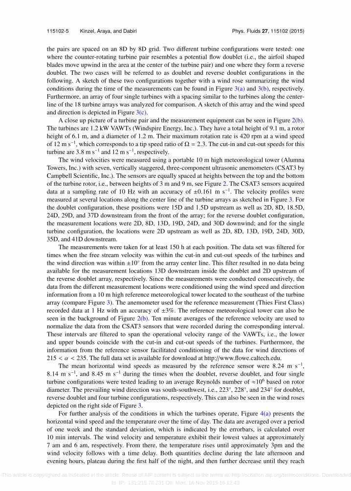
the pairs are spaced on an 8D by 8D grid. Two different turbine configurations were tested: onewhere the counter-rotating turbine pair resembles a potential flow doublet (i.e., the airfoil shapedblades move upwind in the area at the center of the turbine pair) and one where they form a reversedoublet. The two cases will be referred to as doublet and reverse doublet configurations in thefollowing. A sketch of these two configurations together with a wind rose summarizing the windconditions during the time of the measurements can be found in Figure 3(a) and 3(b), respectively.Furthermore, an array of four single turbines with a spacing similar to the turbines along the center-line of the 18 turbine arrays was analyzed for comparison. A sketch of this array and the wind speedand direction is depicted in Figure 3(c).

A close up picture of a turbine pair and the measurement equipment can be seen in Figure 2(b).The turbines are 1.2 kW VAWTs (Windspire Energy, Inc.). They have a total height of 9.1 m, a rotorheight of 6.1 m, and a diameter of 1.2 m. Their maximum rotation rate is 420 rpm at a wind speedof 12 m s−1, which corresponds to a tip speed ratio of Ω = 2.3. The cut-in and cut-out speeds for thisturbine are 3.8 m s−1 and 12 m s−1, respectively.

The wind velocities were measured using a portable 10 m high meteorological tower (AlumnaTowers, Inc.) with seven, vertically staggered, three-component ultrasonic anemometers (CSAT3 byCampbell Scientific, Inc.). The sensors are equally spaced at heights between the top and the bottomof the turbine rotor, i.e., between heights of 3 m and 9 m, see Figure 2. The CSAT3 sensors acquireddata at a sampling rate of 10 Hz with an accuracy of ±0.161 m s−1. The velocity profiles weremeasured at several locations along the center line of the turbine arrays as sketched in Figure 3. Forthe doublet configuration, these positions were 15D and 1.5D upstream as well as 2D, 8D, 18.5D,24D, 29D, and 37D downstream from the front of the array; for the reverse doublet configuration,the measurement locations were 2D, 8D, 13D, 19D, 24D, and 30D downwind; and for the singleturbine configuration, the locations were 2D upstream as well as 2D, 8D, 13D, 19D, 24D, 30D,35D, and 41D downstream.

The measurements were taken for at least 150 h at each position. The data set was filtered fortimes when the free stream velocity was within the cut-in and cut-out speeds of the turbines andthe wind direction was within ±10 from the array center line. This filter resulted in no data beingavailable for the measurement locations 13D downstream inside the doublet and 2D upstream ofthe reverse doublet array, respectively. Since the measurements were conducted consecutively, thedata from the different measurement locations were conditioned using the wind speed and directioninformation from a 10 m high reference meteorological tower located to the southeast of the turbinearray (compare Figure 3). The anemometer used for the reference measurement (Thies First Class)recorded data at 1 Hz with an accuracy of ±3%. The reference meteorological tower can also beseen in the background of Figure 2(b). Ten minute averages of the reference velocity are used tonormalize the data from the CSAT3 sensors that were recorded during the corresponding interval.These intervals are filtered to span the operational velocity range of the VAWTs, i.e., the lowerand upper bounds coincide with the cut-in and cut-out speeds of the turbines. Furthermore, theinformation from the reference sensor facilitated conditioning of the data for wind directions of215 < α < 235. The full data set is available for download at http://www.flowe.caltech.edu.

The mean horizontal wind speeds as measured by the reference sensor were 8.24 m s−1,8.14 m s−1, and 8.45 m s−1 during the times when the doublet, reverse doublet, and four singleturbine configurations were tested leading to an average Reynolds number of ≈106 based on rotordiameter. The prevailing wind direction was south-southwest, i.e., 223, 228, and 234 for doublet,reverse doublet and four turbine configurations, respectively. This can also be seen in the wind rosesdepicted on the right side of Figure 3.

For further analysis of the conditions in which the turbines operate, Figure 4(a) presents thehorizontal wind speed and the temperature over the time of day. The data are averaged over a periodof one week and the standard deviation, which is indicated by the errorbars, is calculated over10 min intervals. The wind velocity and temperature exhibit their lowest values at approximately7 am and 6 am, respectively. From there, the temperature rises until approximately 3pm and thewind velocity follows with a time delay. Both quantities decline during the late afternoon andevening hours, plateau during the first half of the night, and then further decrease until they reach

This article is copyrighted as indicated in the article. Reuse of AIP content is subject to the terms at: http://scitation.aip.org/termsconditions. Downloaded

to IP: 131.215.70.231 On: Mon, 16 Nov 2015 16:12:43

115102-6 Kinzel, Araya, and Dabiri Phys. Fluids 27, 115102 (2015)

FIG. 3. Sketch of the measurement setup (left) and wind rose for the time of the measurement duration (right) for thedoublet (a), reverse doublet (b), and four single turbine (c) configurations. Red circles symbolize counter clockwise rotatingturbines, blue circles clockwise rotating turbines, red crosses the measurement locations, and Xcl is the coordinate along themeasurement transect following the array center line.

This article is copyrighted as indicated in the article. Reuse of AIP content is subject to the terms at: http://scitation.aip.org/termsconditions. Downloaded

to IP: 131.215.70.231 On: Mon, 16 Nov 2015 16:12:43

115102-7 Kinzel, Araya, and Dabiri Phys. Fluids 27, 115102 (2015)

FIG. 4. (a) Horizontal wind velocity (solid) and temperature (dashed) for the time of day. (b) Bulk Richardson number (solid)for the time of day. Errorbars denote one standard deviation.

the before mentioned minimums. The bulk Richardson number is defined as

Ri =g

θv

∂θv∂z(

∂u∂z

)2+(∂v∂z

)2 , (8)

where g is the gravitational constant, θv the potential temperature, and z the vertical direction inwhich the temperature and velocity gradients are calculated. As described in Ref. 4, Ri signalslarge levels of turbulence due to wind shear when it is small and negative. The wind forces arealso dominant when Ri is small and positive. However, in the latter case, the flow is weakly stable.Jacobson4 states the critical Richardson number at which a laminar flow becomes turbulent as 0.25and the termination Richardson number at which turbulent flow turns laminar as 1.0.

Figure 4(b) shows the Richardson number over the time of day. Again the data are averagedover a period of one week. The atmospheric surface layer is weakly stable in the early morninghours with a peak in Ri around 5 o’clock. During the daytime, the flow is turbulent and dominatedby shear from the wind velocities. Ri turns negative around the time when the wind velocities startto increase in the morning and turns positive when the velocities start to decrease in the evening.Considering the cut-in wind speed of the turbines, it can be assumed that the turbines are producingmost of their power at times when the atmospheric surface layer is unstable.

During all measurement campaigns, the power output of each turbine was monitored using aWattNode Modbus (Continental Control Systems LLC). These sensors have an accuracy of ±0.5%when the measured current is between 5% and 100% of the rated current. The accuracy reduces to±1%–3% when the WattNode is operated outside of these boundaries. Similarly to the referencewind data, the turbine power was sampled at 1 Hz and stored as 10 min averages. The powercoefficient, Cp, is a measure of the wind turbine efficiency, i.e., the turbine power output normalizedby the available energy in the flow. This metric is defined as

Cp =Pturbine

12 ρA|U|3 , (9)

where Pturbine is the power output of the respective turbine, ρ is the density of the fluid, A isthe projected area of the turbine, and U is the characteristic wind velocity vector containing thethree velocity components uref , vref , and wref . The characteristic wind velocity is measured by thereference tower outside of the turbine canopy at a height of 10 m, i.e., one meter above the turbinerotors. Therefore, the calculated Cp is more conservative in comparison to the common procedurefor HAWTs where the reference velocity is taken at the center of the rotor. In Sec. III, the energytransfer between the atmospheric surface layer and the turbine canopies is measured by calculatinga power coefficient based on the turbine power output and the energy available in the free stream.Therefore, these power coefficients include the turbine efficiency as well as the efficiency of theenergy transfer between the atmospheric surface layer and the turbine canopy. For the configuration

This article is copyrighted as indicated in the article. Reuse of AIP content is subject to the terms at: http://scitation.aip.org/termsconditions. Downloaded

to IP: 131.215.70.231 On: Mon, 16 Nov 2015 16:12:43

115102-8 Kinzel, Araya, and Dabiri Phys. Fluids 27, 115102 (2015)

of four single VAWTs, the turbines could be calibrated allowing for Cp to capture only the efficiencyof the energy transfer.

III. RESULTS

A. Mean velocity and power

Since the power production of the turbines is proportional to the cube of the streamwisewind velocity, the relationship between these two quantities is analyzed first. Figure 5(a) presentsthe normalized streamwise velocity, u/U, and (b) the average turbine power coefficient, Cp, asmeasured along the center line of the array for the doublet (red), reverse doublet (green), and foursingle turbine (blue) configurations. The velocities were measured at locations roughly 2D in frontof the turbine arrays as well as 2D and 8D downwind from the turbine pairs along the array centerline and at the same distances relative to the single turbines, respectively. Furthermore, there weremeasurements taken 15D upstream and downstream of the 18 turbine array. The exact locations arelisted in Section II.

One observable trend is that the flow velocity decreases to approximately 80% of the freestream velocity as it approaches the turbine array. This is caused by a combination of the blockageeffect of the turbines and the fact that the free stream velocity is measured at a height of 10 mabove ground while the centerline velocity along the array is derived as an average of the sensorsthat are equally spaced between 3 m and 10 m above ground. Each of these effects accounts forapproximately half of the upstream velocity reduction based on the data that were collected at thelocation 15D upstream of the array. Within the array, the streamwise velocity decreases further aseach turbine extracts energy from the flow. The velocity then increases again in the wake region

FIG. 5. (a) Normalized velocity and (b) time averaged power coefficient for the doublet (solid), reverse doublet (dashed),and single (dotted) turbine configurations as well as calibrated power coefficients of the four single turbine configuration(dashed-dotted). Black shapes symbolize turbine positions along array centerlines. Error bars denote one standard deviation.

This article is copyrighted as indicated in the article. Reuse of AIP content is subject to the terms at: http://scitation.aip.org/termsconditions. Downloaded

to IP: 131.215.70.231 On: Mon, 16 Nov 2015 16:12:43

115102-9 Kinzel, Araya, and Dabiri Phys. Fluids 27, 115102 (2015)

of the individual turbines as well as behind the array. For the turbine pairs, the resulting flowvelocities are around 60% of the freestream at 2D and 70% at 8D behind the turbines. The regionbehind the first turbine pair experiences slightly higher flow velocities as it is more exposed to thefreestream flow. Interestingly, the flow only recovers to 70% of the freestream value at the location15D downstream of the 18 turbine array.

For the four single turbines, the flow velocities drop to approximately 50% and recover toaround 75% of the freestream velocity at the positions 2D and 8D behind the turbines, respectively.The lower flow velocity measured immediately behind the single turbines could be attributable tothe fact that the measurement location is located behind the turbine instead of between the twoturbines that make up a pair. A reason for the higher recovery in the wake behind the single turbinesis the lack of blockage that comes from the surrounding turbines in the larger arrays.

Cp is calculated with the freestream velocity U. While this underestimates the efficiency ofthe downstream turbines, it allows to evaluate the performance of the energy transport inside thearray. The energy transport inside the turbine array is the main reason for the changes in Cp sincethe turbine efficiency varies little between the cut-in and cut-out wind velocities. The average Cp

values for each of the four single turbines is calibrated with the turbine Cp measured when thewind was coming from a direction perpendicular to the line of turbines (dashed-dotted line inFigure 5(b)). This was not possible for the turbines along the center line of the 18 turbine arraysdue to the obstruction of adjacent turbines. Therefore, the measured Cp of these turbines dependnot only on the flow but also on the efficiency of the individual turbines, which exhibited smalldifferences attributed to their manufacturing. The calculated Cp is averaged over the two turbines ofa pair in order to lessen this effect. The power production is the lowest for the doublet configurationwith Cp values of 0.128, 0.106, and 0.076 for the turbines of the first, second, and third turbinepairs along the array center line. The respective Cp values for the reverse doublet configuration are0.141, 0.109, and 0.081. While the values of the reverse doublet case are slightly higher than forthe doublet case, the slope of the curves is nearly identical, suggesting that the decay in the flowvelocities inside the arrays is very similar. The Cp curve for the four single turbines on the otherhand decreases less significantly with values of 0.134, 0.123, 0.118, and 0.115. Interestingly, Cp ofthe turbine in the first row of the four single turbines falls right in between the Cp of the turbinesin the first rows of the doublet and reverse doublet configurations. For the doublet configuration, Cp

decreases by 17% between the first and the second and by 28% between the second and third turbinerows. The corresponding values for reverse doublet configuration are 23% and 26%. For the foursingle turbines, Cp decreases 8%, 4%, and 3% between the first, second, and third turbine rows. Thedecreases in power output are consistent with the decreases in the velocities between the areas infront of the first, second, and third turbine rows considering the P ∝ u3 relationship. Since the valueof the streamwise velocity is similar behind the second and third turbine pairs, the power productionof additional rows located further downstream would most likely not decrease as significantly.

Instead of the turbine power coefficients, the power drop between the most upstream turbinesand the corresponding downstream turbines can be calculated in order to analyze the performanceof a turbine array. This method has the disadvantage that the values representing the turbines’performance depend not only on the flow and the efficiency of the turbine that is analyzed but alsoon the efficiency of the most upstream turbine. Mechali et al.5 use this method to investigate the datafrom the Horns Rev HAWT array off the shore of Denmark. This array consists of an 8 by 10 gridof 2 MW Vestas HAWTs with a rotor diameter of 80 m and a hub height of 70 m. The layout ofthis array can be seen in Figure 6(a). The spacing of the turbines is 7D in north-south as well as ineast-west direction resulting in a spacing of 9.9D along the array diagonal. This is similar to the 8Dby 8D spacing of the turbine arrays tested at FLOWE. The spacing of the turbines, which are locatedin pairs in the transverse direction, is smaller resulting in a higher energy density. Mechali et al.5

evaluated three rows with eight turbines each along the array diagonal (222 ± 2) for times whenthe wind velocity was aligned with this direction and between 8 and 9 m s−1. In Figure 6(a), thecorresponding turbines are enclosed by a black rectangle and the arrow indicates the wind direction.This case is similar to the flow along the VAWT array center line at FLOWE. The power curves cor-responding to this wind direction and velocity are presented in Figure 6(b) for the doublet (solid),reverse doublet (dashed), single turbine (dotted), and the HAWT (dashed-dotted) arrays. In contrast

This article is copyrighted as indicated in the article. Reuse of AIP content is subject to the terms at: http://scitation.aip.org/termsconditions. Downloaded

to IP: 131.215.70.231 On: Mon, 16 Nov 2015 16:12:43

115102-10 Kinzel, Araya, and Dabiri Phys. Fluids 27, 115102 (2015)

FIG. 6. (a) Sketch of Horns Rev wind farm. The circles symbolize the turbine positions, the arrow the wind direction of222±2, and the square encloses the three turbine rows for which data was evaluated. (b) Time averaged, normalized powerdata of the doublet (solid), reverse doublet (dashed), and single (dotted) turbine configurations as well as for the Horns Revconfiguration (dashed-dotted) for wind speed between 8 and 9 m s−1. Error bars denote one standard deviation.

to the power coefficient data, these plots show the average power production of the turbines in agiven row along the array diagonal normalized with the average power production of the turbines inthe most upstream row. As a result, the curves for the power drop look slightly different than the cor-responding Cp data. Namely, since the first turbine pair performs better in the reverse doublet thanin the doublet configuration, the power drop for the downstream rows is greater for the former eventhough the Cp of these turbines is higher (compare Figure 5(b)). But in general, it can be observedthat the power drop between the 18 turbine VAWT arrays and the turbines along the diagonal of theHAWT array is very similar especially between the first and the second rows. The power drop seemsto be slightly higher for the VAWT arrays between the second and third rows. The single turbineconfiguration performs significantly better than the larger turbine arrays. This suggests that there isa transverse momentum flux even though the mean wind direction is aligned with the turbines andunderlines the importance of the vertical energy transport in large turbine arrays. It has to be keptin mind that this direct comparison has its limitations as the two different types of turbines operateat different Reynolds numbers, in different areas of the atmospheric surface layer, and in differentterrain. Therefore, the differences in the power output of the downstream turbines do not only resultfrom the differences in the wake structures of HAWTs and VAWTs. Especially, the lower positionin the atmospheric surface layer and the larger roughness length of the surrounding terrain cause ahigher turbulent mixing rate for the VAWTs. Unfortunately, it is not possible to derive a quantitativeestimate for these effects without detailed flow velocity measurements in a HAWT array.

B. Energy transport

The streamwise and planform energy components are analyzed next to gain a better under-standing of the kinetic energy that is available inside of the turbine array. For the streamwise energy

This article is copyrighted as indicated in the article. Reuse of AIP content is subject to the terms at: http://scitation.aip.org/termsconditions. Downloaded

to IP: 131.215.70.231 On: Mon, 16 Nov 2015 16:12:43

115102-11 Kinzel, Araya, and Dabiri Phys. Fluids 27, 115102 (2015)

FIG. 7. (a) Streamwise, (b) planform, and (c) transverse normalized power for the doublet (solid), reverse doublet (dashed),and four single turbine (dotted) configurations. Black lines symbolize turbine positions along array centerlines. Error barsdenote one standard deviation.

transport, the data are averaged over all seven sensors while only the measurements of the topmost sensor is considered for the planform energy component. Figure 7 displays (a) the streamwise,(b) the planform, and (c) transverse energy components normalized with the energy that is avail-able in the free stream, Ps/Pref = u3/u3

ref , Pp/Pref = 2Ap/Asu(u′w ′)/u3

ref , and Pt/Pref = v3/u3ref .

Data are presented for the doublet (solid), reverse doublet (dash), and four single turbine (dot)configurations.

The curves for the streamwise energy behave similar to the velocity curves since Ps ∝ u3.Namely, this component decreases as the turbines take energy out of the flow and then increasesagain in the area of the turbine wakes where new energy is brought in through the planform compo-nent. There is a clear difference in the behavior of the streamwise energy flux for the 18 turbine

This article is copyrighted as indicated in the article. Reuse of AIP content is subject to the terms at: http://scitation.aip.org/termsconditions. Downloaded

to IP: 131.215.70.231 On: Mon, 16 Nov 2015 16:12:43

115102-12 Kinzel, Araya, and Dabiri Phys. Fluids 27, 115102 (2015)

array and the four single turbine configuration. The streamwise energy recovers to more than 90%of the energy in front of the previous turbine in the case of the four single turbines. For the 18turbine array, it only recovers to about 70% behind the first turbine pair and then starts to recoverto about 90% of the value in front of the adjacent upstream turbine pair after that. Furthermore, thestreamwise energy does not recover as quickly behind the 18 turbine array as it does behind the lastturbine of the four single turbines.

As mentioned before, the energy transferred in the area behind the turbines by the transverseand planform energy components increases the energy contained in the frontal component.

Positive levels of Pp represent energy moving into the array from above. The planform mo-mentum flux is higher in the 18 turbine arrays and also spans a larger area because the turbulencefluctuations at the top of the turbine canopy are higher for the larger arrays. This component is ofspecial importance in large wind farms since it is the only transport mechanism bringing energyto the turbines located in the downwind part of the array after the energy that entered the arrayfrom the front and the sides has been depleted. Furthermore, the vertical component of the energytransport depends on the Reynolds stress tensor (Pp ∝ u(u′w ′)) and therefore increases with higherturbulence levels. This explains why its levels spike behind the turbines where the turbulence levelsare highest. Here as well, there is a difference in the behavior of the energy flux between the 18 andthe four single turbine arrays. For the 18 turbine arrays, the planform energy flux increases as theflow approaches the turbine array, declines after the first turbine pair, and then increases to a plateaustarting in front of the second turbine pair. For the four single turbine array, the planform energyis the lowest in front of and highest behind the first turbine. Afterwards it is low in front of, andhigh behind, the consecutive turbines. However, it does not reach the high levels that are exhibitedbehind the first turbine and also remains lower than the plateaus seen within the 18 turbine arrays.While the measurements show that energy is on average entering the turbine array in the verticaldirection, the standard deviation of the planform energy transport is large. This is caused by theturbulence intensity of the flow and suggests that the energy transport is dominated by intense flowevents moving fluid with high or low energy into or out of the turbine array. The flow phenomenainvolved in the vertical energy transport are analyzed and quantified in Sec. III C.

Due to their omni-directionality, VAWTs can also utilize the energy from the transverse mo-mentum flux. However, this is only meaningful in arrays that are small in the transverse direc-tion. The transverse sizes of the arrays under investigation are relatively small, i.e., two orders ofmagnitude smaller than the atmospheric boundary layer. Nevertheless the momentum flux in thetransverse direction is on the same order as the in the planform, see Figure 7(c). The influence ofthe transverse array size becomes apparent when comparing the data for the four single turbineswith that of the two larger arrays. Namely, the transverse momentum flux is approximately twiceas large in the four single turbine configuration. The measurements suggest that the power densityof the arrays in which the turbines are located in pairs is higher compared to the single turbineconfigurations over a wide range of inflow angles. For further details about the influence of theinflow angle on the power production of a VAWT pair see Ref. 19.

C. Quadrant-hole analysis

Because of its importance to the energy transport in large wind farms, the planform energytransport is further studied here. Figure 8 presents the results from the quadrant-hole analysis for the(top) doublet, (middle) reverse doublet, and (bottom) four single turbine configurations. The dura-tion of sweeps, ejections, and inward and outward interactions, Di,H , is given on the left while themagnitude of the normalized Reynolds stresses of these events, Si,H , can be found on the right handside. The solid lines represent the data from the measurement location 15D upstream of the turbinearrays. The dotted line presents the data from a location 2D and the dashed line from a location 8D(7.5D for the doublet configuration) downwind of a turbine pair. The data 2D downwind of a turbinepair was measured at Xcl/D = 24, i.e., behind the third turbine row and the data 8D downwind ofa turbine pair was taken behind the second turbine row, i.e., at Xcl/D = 19 (Xcl/D = 18.5 for thedoublet configuration). Data were used from the area behind different turbine rows because of thelack of data immediately behind the second turbine row for the doublet configuration.

This article is copyrighted as indicated in the article. Reuse of AIP content is subject to the terms at: http://scitation.aip.org/termsconditions. Downloaded

to IP: 131.215.70.231 On: Mon, 16 Nov 2015 16:12:43

115102-13 Kinzel, Araya, and Dabiri Phys. Fluids 27, 115102 (2015)

FIG. 8. (Left) Duration and (right) stress of sweeps (black, Q4), ejections (green, Q2), inward (red, Q1), and outwardinteractions (blue, Q3) for (top) doublet, (middle) reverse doublet, and (bottom) single turbines configurations. Data arepresented for the measurement locations along the array centerlines which are located 15 D upstream (solid) of the array aswell as 2D (dotted) and 8D (dashed) downstream of the turbine pairs. (The presented data were measured 2D behind the 3rdand 8D behind the 2nd turbine rows).

The duration of events appears to be very similar not only between the different turbine config-urations but also between the different measurement locations in front of and within the turbinearrays. However, a slight increase in the duration of ejections and sweeps and decrease in inwardand outward interactions can be seen between the upstream and the positions within the arrays.More significant, however, is the change in the occurrence of Reynolds stress events both betweenthe different turbine configurations and even more so between the locations within each turbinearray.

At the location upstream of the turbine arrays, all four sectors contribute approximately equallyto the Reynolds stress tensor. Only ejections occur slightly more often, which is in agreement with

This article is copyrighted as indicated in the article. Reuse of AIP content is subject to the terms at: http://scitation.aip.org/termsconditions. Downloaded

to IP: 131.215.70.231 On: Mon, 16 Nov 2015 16:12:43

115102-14 Kinzel, Araya, and Dabiri Phys. Fluids 27, 115102 (2015)

the findings of Belcher et al.22 Within the turbine arrays, however, the occurrence of ejections and,to a slightly lower extent, sweeps increases. Belcher et al.22 also report an increase in ejections inthe transition region from an atmospheric surface layer to a canopy flow.

The highest increase can be seen in the ejections measured at the location 2D behind theturbines. The values are similar between the different configurations with the highest levels recordedfor the four single turbines followed by the reverse doublet and then the doublet configurations.While the occurrence of ejections remains almost constant between the 2D and 8D locations in thelarger arrays, it decreases almost to the level measured upstream of the arrays for the four singleturbine configuration.

FIG. 9.Si,H

uref

2dH for (a) the doublet, (b) reverse doublet, and (c) the single turbine configurations where (red)

lines represent outward interactions, (blue) inward interactions, (green) ejections, and (black) sweeps. Black lines symbolizeturbine positions along array centerlines.

This article is copyrighted as indicated in the article. Reuse of AIP content is subject to the terms at: http://scitation.aip.org/termsconditions. Downloaded

to IP: 131.215.70.231 On: Mon, 16 Nov 2015 16:12:43

115102-15 Kinzel, Araya, and Dabiri Phys. Fluids 27, 115102 (2015)

Sweeps also exhibit a higher occurrence at the location 2D behind the turbines. While the levelsare again very similar between the different configurations at this measurement position, this is notthe case further downstream. For the larger arrays, the occurrence of sweep events is even higher at8D downstream from the turbine pairs than at 2D, while it is almost identical to the upstream valuesfor the four single turbine configuration.

The observation that the occurrence of ejections and sweeps remains elevated within the 18turbine arrays, whereas it goes down to almost the upstream levels for the four single turbine config-uration is in agreement with earlier observations about the behavior of Pp (compare Figure 7(b)).

The impact on inward and outward interactions is not as pronounced. The occurrence of bothdecreases inside the turbine arrays in comparison to the location 15D upstream. Only for the doubletconfiguration at the locations 8D behind the turbines and for low H events do they increase.

The plots from the quadrant-hole analysis in Figure 8 represent the flow phenomena at a singlemeasurement location. To achieve a quantitative understanding of the effect of sweeps, ejections,and outward and inward interactions over the whole area of each turbine array, the conditionedReynolds shear stress of each quadrant was integrated over H. Thus,

Si,H/u

2ref dH represents the

normalized amount that ejections, sweeps, and inward and outward interactions contribute to theenergy transport at the analyzed measurement location. Figure 9 presents the corresponding curvesfor (a) the doublet, (b) the reverse doublet, and (c) the four single turbine configurations. Outwardinteractions (red) and inward interactions (blue) are positive as they are transporting energy upwardswhile ejections (green) and sweeps (black) are negative, transporting energy downwards into theturbine canopy.

For all turbine arrays, the amount of energy that is transported downwards is higher than theamount that is leaving the array at the top. Additionally, ejections are the highest contributor to theplanform energy transport followed by sweeps in all cases.

These plots indicate that for the 18 turbine arrays, the amount of energy transported by ejec-tions and sweeps increases and reaches a plateau behind the second turbine pair. The contribution ofinward and outward interactions on the other hand decreases and also reaches a plateau behind thesecond turbine pair. Exceptions are spikes in inward and outward interactions as well as the sweepsaround the first turbine pair in the doublet configuration. A possible explanation for this increase inthe Reynolds stresses is the exposed position of these first turbine pairs in front of the arrays.

For the four single turbine configuration, inward and outward interactions remain nearly con-stant throughout the turbine array. Ejections and sweeps do not exhibit the same kind of plateauregion that is visible for the larger turbine arrays. Instead, both experience spikes behind the tur-bines but then fall down to a lower level with downstream distance. The magnitude of the spikes isslightly higher than that of the plateau regions in the 18 turbine arrays.

IV. CONCLUSIONS

Measurements of the streamwise velocity show that the blockage effect of all three turbinearrays is similar at approximately 10%. While this is not surprising when looking at the two 18turbine arrays, it is noteworthy that an array with three turbine pairs in the transverse direction cre-ates the same effective blockage in the streamwise direction as four single turbines in a row. Withinthe turbine arrays, the streamwise velocity suggests how the turbines extract energy from the flowand how the energy is replenished in the wake region behind the turbine. As would be expected,the flow recovers more rapidly behind the turbines in the four single turbine configuration. This isespecially apparent in the region behind the turbine arrays where the flow recovers to only 70%of the reference streamwise velocity at the measurement location 15D downwind of the 18 turbinearray while it recovers to 80% at the location 8D behind the four single turbine configuration.

The trend in the power coefficients of the turbines are in agreement with the data from thestreamwise velocity measurements. While Cp decreases form the first to the second and the secondto the third turbine pair in the 18 turbine arrays, it remains nearly constant between the turbines inthe four single turbine configuration. However, the velocity measurements behind the third turbinepair suggest that the power output of consecutive pairs would be close to that of the third pair. It

This article is copyrighted as indicated in the article. Reuse of AIP content is subject to the terms at: http://scitation.aip.org/termsconditions. Downloaded

to IP: 131.215.70.231 On: Mon, 16 Nov 2015 16:12:43

115102-16 Kinzel, Araya, and Dabiri Phys. Fluids 27, 115102 (2015)

appears that the turbines in the reverse doublet configuration perform slightly better than those inthe doublet configuration with Cp of the turbine pair in the first row being close to that of the singleturbine configuration. However, due to the uncertainties associated with field measurements and thesmall difference between the performance of the two 18 turbine configurations, this is speculativepending further study.

The comparison between the normalized power data from the three VAWT arrays and HAWTdata from Horns Rev suggests that within large arrays, the power drop between downstream tur-bines is similar between the two turbine types. However, placing the VAWTs in pairs increases thepower density of the turbine array compared to HAWTs. This observation is interesting since thewake analysis of isolated vertical axis and horizontal axis turbines suggests that the flow recoversfaster behind VAWTs. This faster recovery can be seen in the four single turbine configuration.Further study is needed because while both types of turbine arrays were spaced similarly in thedownstream direction in terms of rotor diameter, the respective turbines were operated at differentReynolds numbers and in different parts of the atmospheric surface layer.

Evaluating the streamwise and planform components of the momentum flux highlights theimportance of the planform energy transport for large wind farms. While the streamwise energytransport is dominant in the upstream rows of the array, the planform component brings new energyfor the downstream turbines. This is especially important since the transverse component seems todecrease quickly with the turbine array size in this direction. The planform component is higher forthe 18 turbine arrays than for the four single turbine configuration. This is most likely due to thehigher turbulence levels at the top of the larger turbine canopy and will therefore only increase withthe turbine array size until the flow along the center line has fully adjusted to the new roughnesslength that is caused by the turbines.

The planform momentum flux was analyzed further using quadrant-hole analysis. The resultssuggest that there is an analogy between the flow in a dense VAWT array and a plant or urbancanopy. That is, they show an increase in ejections and sweeps as well as a decrease in inwardand outward interaction events. A key finding is the difference in the occurrence of these flowphenomena between the 18 turbine arrays and the four single turbine configuration. For the largerarrays, ejections and sweeps are increased and inward and outward interactions decreased both atthe measurement locations 2D and 8D behind the turbines. However, in the four single turbine array,this increase and decrease in the quadrant events is only pronounced at the measurement locationclose to the turbines and mainly involves an increase in ejections. This suggests again that a newsurface layer flow evolves on top of the 18 turbine array while the flow between the four singleturbines recovers close to the surface layer flow found upstream of the turbines. This differencebetween the turbine configurations is further highlighted by looking at the product of the occurrenceand the Reynolds stress terms, Si,HDi,H , over the whole length of the array centerlines. For the 18turbine arrays, the magnitude of these flow events changes in the first two turbine rows and then pla-teaus. For the four single turbine configuration, the magnitude of these flow events keeps increasingand decreasing depending on whether the measurement location is close to or further away from aturbine. These results also underline the finding that ejections are the strongest mechanism for theenergy transport in the transition area of the turbine canopy, followed by sweeps and that inward andoutward interactions occur less often in comparison to the upstream flow.

These findings show a strong similarity between the flow in VAWT arrays and the adjustmentregion of canopies. They suggest that a dense spacing of VAWTs can lead to an increase in theplanform energy flux over the whole planform area of the turbine array. However, further research isnecessary to derive quantitative models for the prediction of the planform energy transport in VAWTarrays based on the current models for canopy flows.

ACKNOWLEDGMENTS

The authors gratefully acknowledge funding from the Gordon and Betty Moore Foundationthrough Grant No. 2645, the National Science Foundation Energy for Sustainability program (GrantNo. CBET-0725164), and the Office of Naval Research through Grant No. N000141211047.

This article is copyrighted as indicated in the article. Reuse of AIP content is subject to the terms at: http://scitation.aip.org/termsconditions. Downloaded

to IP: 131.215.70.231 On: Mon, 16 Nov 2015 16:12:43

115102-17 Kinzel, Araya, and Dabiri Phys. Fluids 27, 115102 (2015)

1 S. Frandsen, “On the wind speed reduction in the center of large clusters of wind turbines,” J. Wind Eng. Ind. Aerodyn. 39,251–265 (1992).

2 J. Meyers and C. Meneveau, “Optimal turbine spacing in fully developed wind farm boundary layers,” Wind Energy 15,305 (2011).

3 B. Newman, “The spacing of wind turbines in large arrays,” J. Energy Convers. 16, 169–171 (1977).4 M. Z. Jacobson, Fundamentals of Atmospheric Modeling (Cambridge University Press, 2005).5 M. Méchali, R. Barthelmie, S. Frandsen, L. Jensen, and P. E. Réthoré, “Wake effects at Horns Rev and their influence

on energy production,” in Proceedings of the 2006 European Wind Energy Association Conference in Athens, Greece(Curran Associates, 2006), pp. 570–580, ISBN: 9781622764679.

6 X. Yang, S. Kang, and F. Sotiropoulosa, “Computational study and modeling of turbine spacing effects in infinite alignedwind farms,” Phys. Fluids 24, 115107 (2012).

7 R. B. Cal, J. Lebrón, L. Castillo, H. S. Kang, and C. Meneveau, “Experimental study of the horizontally averaged flowstructure in a model wind-turbine array boundary layer,” Renewable Sustainable Energy 2, 013106 (2010).

8 M. Calaf, C. Meneveau, and J. Meyers, “Large eddy simulation study of fully developed wind-turbine array boundary layers,”Phys. Fluids 22, 015110 (2010).

9 L. P. Chamorro, R. E. A. Arndt, and F. Sotiropoulos, “Turbulent flow properties around a staggered wind farm,” BoundaryLayer Meteorol. 141, 349–367 (2011).

10 C. VerHulst and C. Meneveau, “Large eddy simulation study of the kinetic energy entrainment by energetic turbulent flowstructures in large wind farms,” Phys. Fluids 26, 025113 (2014).

11 M. Toloui, S. Riley, J. Hong, K. Howard, L. P. Chamorro, M. Guala, and J. Tucker, “Measurement of atmospheric boundarylayer based on super-large-scale particle image velocimetry using natural snowfall,” Exp. Fluids 55, 1737 (2014).

12 M. Kinzel, Q. Mulligan, and J. O. Dabiri, “Energy exchange in an array of vertical-axis wind turbines,” J. Turbul. 13, 1–13(2012).

13 E. Hau, Wind Turbines (Springer Verlag, Berlin, Heidelberg, 2006).14 R. J. Barthelmie, S. C. Pryor, S. T. Frandsen, K. S. Hansen, J. G. Schepers, K. Rados, W. Schlez, A. Neubert, L. E. Jensen,

and S. Neckelmann, “Quantifying the impact of wind turbine wakes on power output at offshore wind farms,” J. Atmos.Oceanic Technol. 27, 1302–1317 (2010).

15 K. Johnson and N. Thomas, “Wind farm control: Addressing the aerodynamic interaction among wind turbines,” inProceedings of the 2009 American Control Conference in St. Louis, MO (IEEE, 2009), pp. 2104–2109.

16 D. Madjidian, K. Martensson, and A. Rantzer, “A distributed power coordination scheme for fatigue load reduction in windfarms,” in Proceedings of the 2011 American Control Conference in San Francisco, CA (IEEE, 2011), pp. 5219–5224.

17 J. Aho, A. Buckspan, J. Laks, P. Fleming, Y. Jeong, F. Dunne, M. Churchfield, L. Pao, and K. Johnson, “A tutorial ofwind turbine control for supporting grid frequency through active power control,” in Proceedings of the 2012 AmericanControl Conference in Montreal, QC (IEEE, 2012), pp. 3120–3131.

18 R. W. Whittlesey, S. Liska, and J. O. Dabiri, “Fish schooling as a basis for vertical axis wind turbine farm design,” Bioin-spiration Biomimetics 5, 035005 (2010).

19 J. O. Dabiri, “Potential order-of-magnitude enhancement of wind farm power density via counter-rotating vertical-axis windturbine arrays,” J. Renewable Sustainable Energy 3, 043104 (2011).

20 W. Zhu, R. van Hout, and J. Katz, “PIV measurements in the atmospheric boundary layer within and above a Mature CornCanopy. Part II: Quadrant-hole analysis,” J. Atmos. Sci. 64, 2825–2838 (2006).

21 G. Katul, D. Poggi, D. Cava, and J. Finnigan, “The relative importance of ejections and sweeps to momentum transfer inthe atmospheric boundary layer,” Boundary Layer Meteorol. 102, 367–375 (2006).

22 S. E. Belcher, N. Jerram, and J. C. R. Hunt, “Adjustment of a turbulent boundary layer to a canopy of roughness elements,”J. Fluid Mech. 488, 369–398 (2003).

23 S. Lu and W. W. Willmarth, “Measurements of the structure of the Reynolds stress in a turbulent boundary layer,” J. FluidMech. 60, 481–511 (1973).

24 W. Yue, C. Meneveau, M. B. Parlange, W. Zhu, R. van Hout, and J. Katz, “A comparative quadrant analysis of turbulencein a plant canopy,” Water Resour. Res. 43, W05422, doi:10.1029/2006WR005583 (2007).

This article is copyrighted as indicated in the article. Reuse of AIP content is subject to the terms at: http://scitation.aip.org/termsconditions. Downloaded

to IP: 131.215.70.231 On: Mon, 16 Nov 2015 16:12:43