Embed Size (px)
Citation preview
CONTRACTOR REPORT
SAND89-7154 Unlimited Release UC-414
"8232-2 lo^n'3^
8232-2//069932 8232-2//069932
00000001 - 00000001
Dynamics of Plasma Injection Along Magnetic Field Lines in the PBFA II Plasma Opening Switch
Michael H. Frese NumerEx 1400 Central SE, Suite 3200 Albuquerque, NM 87106-4811
Prepared by Sandia National Laboratories Albuquerque, New Mexico 87185
and Livermore, California 94550 for the United States Department of Energy
under Contract DE-AC04-76DP00789
Printed November 1989
Issued by Sandia National Laboratories, operated for the United States Department of Energy by Sandia Corporation. NOTICE: This report was prepared as an account of work sponsored by an agency of the United States Government. Neither the United States Govern¬ ment nor any agency thereof, nor any of their employees, nor any of their contractors, subcontractors, or their employees, makes any warranty, express or implied, or assumes any legal liability or responsibility for the accuracy, completeness, or usefulness of any information, apparatus, product, or process disclosed, or represents that its use would not infringe privately owned rights. Reference herein to any specific commercial product, process, or service by trade name, trademark, manufacturer, or otherwise, does not necessarily constitute or imply its endorsement, recommendation, or favoring by the United States Government, any agency thereof or any of their contractors or subcontractors. The views and opinions expressed herein do not necessarily state or reflect those of the United States Government, any agency thereof or any of their contractors.
Printed in the United States of America. This report has been reproduced directly from the best available copy.
Available to DOE and DOE contractors from Office of Scientific and Technical Information PO Box 62 Oak Ridge, TN 37831
Prices available from (615) 576-8401, FTS 626-8401
Available to the public from National Technical Information Service US Department of Commerce 5285 Port Royal Rd Springfield, VA 22161
NTIS price codes Printed copy: A03 Microfiche copy: A01
SAND89-7154 Distribution Unlimited Release Category UC-414
Printed November 1989
Dynamics of Plasma Injection Along Magnetic Field Lines in the FBFA II Plasma Opening Switch
Michael H. Frese
NumerEx 1400 Central SE, Suite 3200
Albuquerque, New Mexico 87106-4811
Sandia Contract No. 40-0128

Contents
List of Figures 1
2
3
4
5
5.1
5.2
5.3 6
References . . .
Appendix A
Appendix B
Summary ................. Problem Description .......... Computational Difficulty
....... Computational Method ........ Computational Results ........ Low Density Case............ High Density Case
........... One-sided Injection Case ....... Conclusions and Recommendations
Historian Change File to Implement Rigid Field Lines in MACH2 v8801
............................. MACH2 Input File for MIP Simulation Low Density Case
List of Figures
Figure 1
Figure 2
Figure 3
Figure 4
Figure 5
Figure 6
Figure 7
Figures
Figure 9
Figure 10
Figure 11
Figure 12
Figure 13
Figure 14
Figure 15
Figure 16
Figure 17
Computational grid fitting experimental configuration for magnetically controlled plasma injection. Dots mark location of
simulation density probes......................... 8
Magnetic field for control of plasma injection. ...........
9
Density at the end of the mass injection pulse. Low density
case. ...................................... 14
Velocity at the end of the mass injection pulse. Low density case. ......................................
14
Density at 5 /is after the start of the mass injection pulse. Low density case. ................................
15
Velocity at 5 /zs after the start of the mass injection pulse. Low density case. ................................
15
Electron density vs. time at the simulation density probe locations and at one microwave interferometer location. Low density case. ................................ i6 Density at the end of the mass injection pulse. High density
case. ..................................... 17
Velocity at the end of the mass injection pulse. High density case. .....................................
17
Density at 5 ^s after the start of the mass injection pulse. High density case. ................................
18
Velocity at 5 p.s after the start of the mass injection pulse. High density case. ................................
18
Electron density vs. time at the simulation density probe locations. High density case. .....................
19
Density at the end of the mass injection pulse. One-sided injection case. ...............................
20
Velocity at the end of the mass injection pulse. One-sided
injection case. ............................... 21
Density at 5 (is after the start of the mass injection pulse. One-sided injection case. ........................
21
Velocity at 5 p.s after the start of the mass injection pulse.
One-sided injection case. ........................ 22
Electron density vs. time at the simulation density probe
locations. One-sided injection case. ................. 22
1. Summary In the magnetically injected plasma (MIP) plasma opening switch (POS) presently
under study for use on the Particle Beam Fusion Accelerator II (PBFA II), plasma is injected along an imposed poloidal field to control the position of the plasma. The magnetic field and the plasma density combine to make the Alfven velocity very high
relative to the injection velocity of the plasma. In fact, the ratio of these velocities, the Alfven-Mach number of the flow, ranges from 0.001 to 0.01. Explicit computation at these low Mach numbers is exceedingly tedious, and implicit computation without a very high convergence rate scheme is little better. However, the physical effect is clear: the field lines are effectively very stiff" and not subject to displacement by the plasma. The plasma motion may thus be computed by simply restricting the velocity to lie along the field. Simulations in the true experimental geometry using this approach agree qualitatively with microwave interferometry measurements of the plasma density in the experimental tost stand. The agreement is quantitative, subject only to the adjustment of the unknown plasma source mass flux rate.
2. Problem Description
The POS region in PBFA II is geometrically complex, lying between two conical
electrodes, and the MIP modifications further complicate the geometry. Figure 1
shows a computational grid that fits the biconic switch region and the adjacent semi- toroidal plasma source region. The accelerator power pulse travels from the adder located out of the picture to the upper right, down to the load at the lower left.
This grid1 was generated by MACH2, a 2^-D magnetohydrodynamics (MHD) code that creates and computes on multiblock boundary-fitted arbitrary quadrilat¬ eral grids. Further details on MACH2 maybe found in [1]. The experimental region is cylindrically symmetric. The geometric flexibility and power of MACH2 makes it feasible to compute with such a relatively small number of cells, since the boundary conditions can be more accurately applied along grid lines that parallel the physical boundaries. No more spatial resolution is required, since the experimental diagnos¬ tics have even less resolution than this grid.
' The locations of the essential points necessary to generate the computational grid were extracted from the CAD
representation of actual MIP POS hardware by M. Slattery.

MIP - DIFF + IOEJLL T • 3.018B-07 CYCLX • 163 CA.LCOLA.TIOM MZ3H
MIP92
13T Z
X INC 1ST Y
y me
1.50X-01 5
. OOB-02 1 .508-01 5.OOX-02
Figure 1 Computational grid fitting experimental configuration for magnetically controlled plasma injection. Dots mark location of simulation density probes.
A coil carrying from 50 to 200 kiloamp-tums of current in the toroidal direction lies in the small D-shaped hole surrounded by the computational region. The
magnetic field that results from this current is shown in Figure 2. This field is computed using MACH2's multigrid implicit resistive diffusion module. The
equations are advanced approximately 1000 cell diffusion times in 100 timesteps. The boundary conditions used are n • B = 0 on surfaces representing conducting
boundaries, and B = fio^t on the region boundary surrounding the coil. Here I is
the total current in the coil in amp-turns, I is the arc length of the curve in the computational plane surrounding the coil, and t is the tangent vector to that curve. Since I is about 6 cm, the resulting field has a maximum of approximately 2.5 T.
KIP - ozrr + IDEAL T - 2.018E-07 CYCLE MAGNETIC riELO
MAX « 2.564E+00
163 MIP92
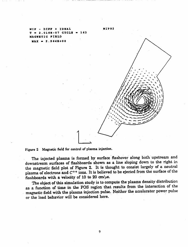
Figure 2 Magnetic field for control of plasma injection.
The injected plasma is formed by surface flashover along both upstream and
downstream surfaces of nashboards shown as a line sloping down to the right in the magnetic field plot of Figure 2. It is thought to consist largely of a neutral plasma of electrons and C4"1" ions. It is believed to be ejected from the surface of the nashboards with a velocity of 10 to 20 cxa/fis.
The object of this simulation study is to compute the plasma density distribution
as a function of time in the POS region that results from the interaction of the
magnetic field with the plasma injection pulse. Neither the accelerator power pulse
or the load behavior will be considered here.

3. Computational Difficulty As MACH2 implements resistive MHD, a one-fluid model of plasma dynamics,
zero is an unsatisfactory value for the density. Hence, the computational region is initially filled completely with a neutral plasma of electron density 2 x IC^cm'"3 which is approximately the density of the residual gas left by the vacuum pumping on PBFA II. This density must be sufficiently small that it has little effect on the dynamics of the injected plasma; it was chosen to be two orders of magnitude smaller than the density of the actual plasma of interest.
The velocity of Alfven waves at this density and field strength is 3 x 10⁷ m/s. Since the grid spacing near the coil is approximately 3 mm, the transit times for these waves is only 1 x 10~10 seconds, and hence the explicit time step required would be 2 — 5 x 10~11 seconds. For the 5 to 10 f^s the plasma takes to reach and fill the switch region, the explicit full MHD computation would require 1 - 5 x 10⁵
timesteps. For this particular problem, that is an unacceptable computer expense.
The implicit algorithm for the MHD in MACH2 can be pushed to take timesteps
an order of magnitude greater, but the cost is a factor of five in computer time per timestep. Thus the payoff is only a factor of two2, and that would still leave the
problem too expensive to solve.
Clearly, the problem is that the field lines are very stiff. Transverse velocities
produce large restoring forces and high opposing accelerations. In fact, the difference
equations are themselves stiff in the sense of the word used in numerical analysis. There are two widely different time scales: one for the transverse plasma motions and another for the parallel. In the recognition of this lies the solution. By removing the short time scale from the problem, the computations may be made to proceed
at the longer one.
2 The reason the payoff is no better is that Jacobi iteration is employed to solve the implicit equations. A multigrid convergence acceleration scheme could pay handsome dividends here.
10

4. Computational Method
Since there is no toroidal field in the problem, the easiest way to remove the short
time-scale motions is to simply remove all magnetohydrodynamic influence of the
plasma on the magnetic field and all magnetic force on the plasma. The incorporation of a simple multiplier in the routines where these influences are applied removes them when the multiplier is set to zero. MACH2 is an Arbitrary Lagrangian/Eulerian code and hence has a time-split implementation of the transport and force equations, so that care must be taken to remove all influences. An additional routine projects the velocity onto the magnetic field everywhere within the computational region. The plasma then moves hydrodynann cally under the action of its own pressure and momentum, and of course the numerical diffusion, along the magnetic field lines.
The HISTORIAN change file necessary to implement these changes in the v8801
version of MACH2 is included here as Appendix A. It is 235 lines long, but contains modifications to the circuit model unnecessary for the plasma injection simulations.
This approach produces a simulation requiring only 400 timesteps to reach 10 ^s
of physical time and less than 3 CRAY XMP CPU-minutes. Simulations of this size
are very effective for design work.
11
5. Computational Results
Three simulations will be discussed in turn in the subsections to follow. The first simulation gives the best comparison with experiment. The other simulations
were performed to assess the importance of the fluid pressure on the dynamics of the injected plasma. The second differs from the first only in that the inflow density is four times greater. The conditions of the third simulation are the same as the
second except that the mass inflow from the downstream side of the flashboard is
not present.
In general, the simulation results are dominated by the relatively shorter path lengths along the more highly curved field lines nearer the coil (see Figure 2). Plasma first arrives in the switching region immediately to the left of the coil. The plasma injected along field lines near the coil from the upstream side of the flashboard meets that from the downstream side and stagnates, creating a peak of density there at about 2 p.s. The plasmas from the upstream and downstream sides on the field lines
farthest from the coil do not meet in the switching region till 5 fis and the peak in the density near the cathode is at approximately this time.
An ideal gas equation of state for a C1'1"1" plasma is used in the simulations. The
plasma pulse is simulated by specifying a constant inflow density and time varying velocity normal to the flashboards. The pulse is sinusoidal, beginning at the end of
the diffusion period, and lasting a single half-period of 100 ns. The figures below that refer to the end of the plasma pulse show the velocity field and the density contours
at the end of that time. In all three cases the injection velocity peaks at 10 cm/fis.
The MACH2 input file for the first simulation is included in this report as
Appendix B. The input files for the others differ only slightly from that one.
The simulation results will be given using contour plots of electron density and vector plots of plasma velocity such as in Figures 3 and 4. In all plots the problem time and cycle are given in the upper left comer. In the contour plots the contour levels are linearly spaced between the maximum and minimum values of the quantity contour plotted, and are indicated in the upper left comer of the plot, along with the
maximum and minimum value. The value associated with the longest vector in each
vector plot is given in the upper left comer, and the length of that vector is shown in the lower left for comparison.
5.1 Low Density Case
The inflow electron density in this case is set to 5 x lO^cm"3 but because of the flow dynamics the largest values reached in the computational region are slightly less than that. The density of the injected plasma reaches only 3 x lO^cm"3. This
value occurs just off the flashboard surface at the end of the plasma pulse near the
12
coil end of the board. The velocity peaks at approximately 8 cm/^s, also just after the end of the pulse.
The density contour lines and the velocity field of the plasma at 200 ns, the end of the injection pulse, are shown in Figures 3 and 4. The peak density at this time is located near the coil end of the fiashboard. The TnanmiiTn plasma velocity is
approximately 8 cm//xs, and all velocities are, of course, parallel to the magnetic field.
Figures 5 and 6 show the density and velocity at 5 /is. By this time, the two plasma clouds coming from opposite sides of the flashboards are already bouncing back toward the flashboards near the coil, though they are only beginning to slow
near the cathode. The double peak in the density results because the plasma that has reversed course along the field lines after meeting in the transmission line is
meeting the oncoming tail of plasma.
The electron number density at the density probe locations (marked by the dots
in Figure 1) is plotted versus time in Figure 7. The density near the anode peaks first, at approximately 2 fiS, while the density near the cathode peaks slightly after 6 fis. The peak density near the cathode, 6 x lO^cm"3, is approximately half the peak near the anode.
For comparison, Figure 7 also shows the experimental range of density measured by Weber [2] near the cathode in the laboratory test stand using microwave inter- ferometry. This measurement was taken approximately 2 cm downstream of the cathode simulation density probe location shown in Figure 1. The lower edge of the
gray region is the density vs. time for a shot with 16 kA-tums of coil flux, and the
upper edge is the density vs. time for a shot with 47 kA-tums of coil flux. These coil fluxes are significantly lower than those that will be used on PBFA II and at these levels, the measured density increases with flux. Weber reports that at other locations this increase saturates at slightly higher flux levels.
The favorable comparison of this simulation result with experiment is somewhat fortuitous, since the density of mass injection was selected rather arbitrarily. As
the simulation preceded the experiment, the author submits that all congratulations
on this good fortune should be conferred upon Dr. Weber and his experimental
colleagues. The fact that the experiment followed the simulation is the reason that the locations of the simulation density probes diner from those of the microwave
interferometry diagnostics.
13
Mir - oxrr + IDSA& Mip»2 T • 2.024X-07 CTCLX - 152 KLBCTROB* / CC
— 2.01+11 A- 5.41+12 •• 1.1B+13
C- l.CI+13 D- 2.11+13 I- 2.CC+13
+- 3.11+13
Figure 3 Density at the end of the mass injection pulse. Low density case.
MIf - Din + IDCA.L Mir»2 T - 2.0341-07 CXCLI • 152 VILOCITI
MU - 7.70M+04
Figure 4 Velocity at the end of the mass injection pulse. Low density case.
14

Mir - Birr + IDKXL Ni»»2 T • 5.002X-OC CICLt - 331 XLKCTSLOir / CC
— 1.01+11 A- 2.4C+12 •• 4.CK+12
C- C.9C+12 D- S.2C+12 X- l.lt+13 +- 1.41*13
Figure 5 Density at 5 ^s after the start of the mass injection pulse. Low density case.
Mzr - ozrr + IOIAI. Mi»«2 T • S.002X-0( CSC&B • 331 VILOCZTZ
MJLX • a.HOB+04
Figure 6 Velodty at 5 fis after the start of the mass injection pulse. Low density case.
15
'-'0246 Time Qis)
Figure 7 Electron density vs. time at the simulation density probe locations and at one microwave interferometer location. Low density case.
5.2 High Density Case
In order to assess the effects of the fluid pressure, this simulation was run with the inflow density increased by factor of four.
The density contour lines and the velocity field of the plasma at the end of the
injection pulse are shown in Figures 8 and 9. They are very similar to the previous case except that the peak density is approximately 4 times higher, and the velocity is slightly greater.
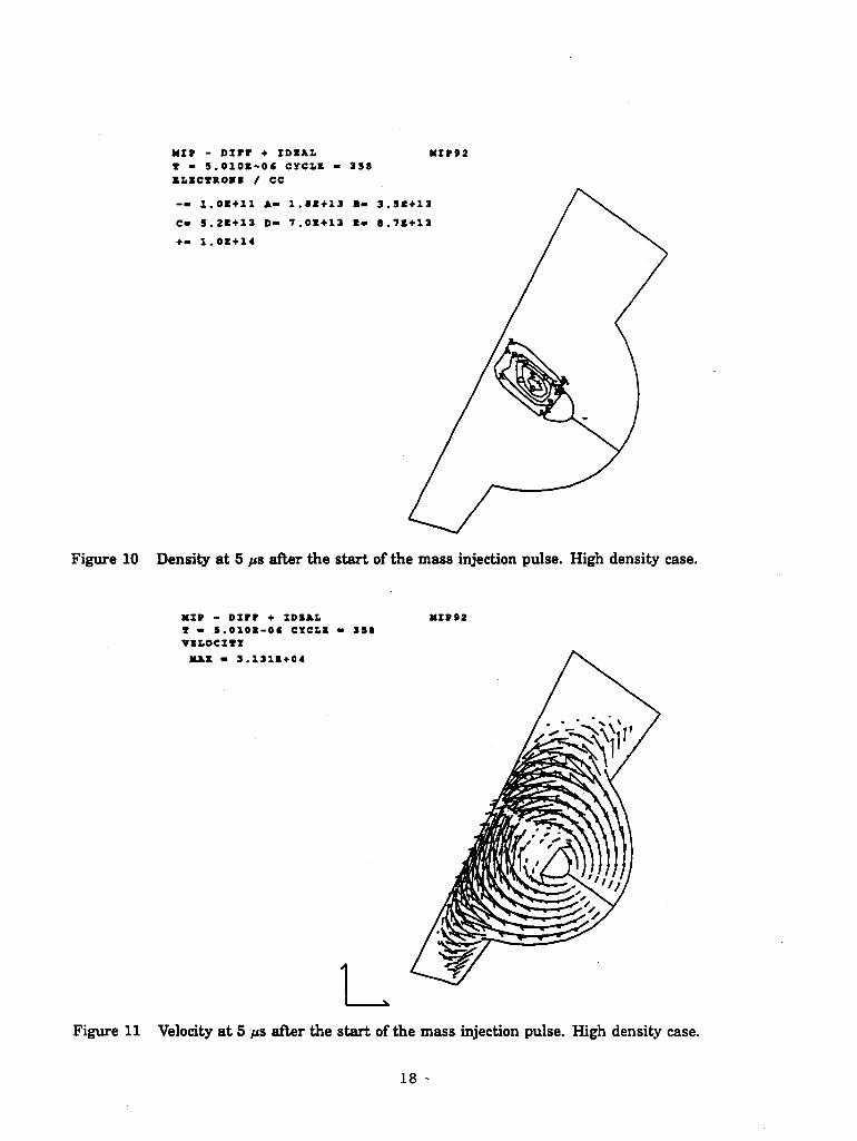
Figures 10 and 11 show the density and velocity at 5 p,s. The plasma on field
lines near the anode is not bouncing back as much in this simulation, and the mass density is more concentrated.
The electron number density at the simulation density probe locations is plotted
versus time in Figure 12. The peak density near the cathode is approximately 4
times as great as in the low density case, while at the anode it is somewhat more than four times as great. Comparison of this figure with Figure 7 shows that the
pulse near the anode is somewhat later and its shape somewhat broader in this case.
16
KIP - Dirr + XOKAL Mir»2 T • 2.0191-07 CYCLl - 163 CLKCTROBI / CC
— 2.0B+11 X« 2.11*13 B- 4.2K+13 C- «.3C+13 D- 8.41+13 C- l.OK+14
+- 1.3C+14
Figure 8 Density at the end of the mass injection pulse. High density case.
MI» - Oirr + ZDIX& MX>»3 T • 2.0rS-07 CTCLI • 1C1 VBLOCITZ
MAX - l.fl+04
Figure 9 Velocity at the end of the mass injection pulse. High density case.
17
NIf - OZrr + IDEAL MIP92 T - 5.010K-OC CYCLl - 358 SLKCTKOXI / CC
— 1.01+11 A- 1.81+13 •• 3.SI+13 C- 5.21+13 0> 7.0B+13 •• 8.71+13 +• 1.01+14
Figure 10 Density at 5 ps after the start of the mass injection pulse. High density case.
MIf - DZrr + IDXAL T • 5.010X-OC CXC&1 - 3S« VILOCITl
MAX - 3.1311+04
MIPB2
Figure 11 Velocity at 5 ps after the start of the mass injection pulse. High density case.
18 '

0 2 4 6 8 10 Time (us)
Figure 12 Electron density vs. time at the simulation density probe locations. High density case.
5.3 One-sided Injection Case
Fluid flows in which the internal energy is small compared to the kinetic energy are very similar to free-streaming particle flows. In order to further assess the collisional effects, this simulation was run with the mass inflow from the downstream side of the flashboard suppressed. Since the injected plasma does not collide with its counterpart from the other side of the flashboard, it is not shock heated, and its
temperature remains less than 5 eV in the transmission line. The density in the
actual experiment in which the two plasmas interpenetrate could be determined by adding the density from this simulation to that from another in which the plasma is injected from the downstream side of the flashboard only. Since the configuration is nearly symmetric, directly between the coil and the cathode, that sum should be
approximately twice the density here. This simulation is of further interest since obstructing the flow from one side of
the flashboard is an easy way to lower the mass of the switch plasma. It also could
reduce the amount of plasma that might be lost across the field lines toward the
load. Since density probe information was not obtained downstream of the coil in these simulations, they do not address that issue.
The density contour lines and the velocity field of the plasma at the end of the
injection pulse are shown in Figures 13 and 14. They are very similar to the previous
case.
19

Figures 15 and 16 show the density and velocity at 5 p,s. The plasma on field
lines near the coil has piled up against the opposite side of the flashboard from which it was emitted. The plasma on field lines near the cathode fills the transmission line. The picture of the density that this gives is significantly different from that of the high density simulation, but not so different from that of the low density one. It is likely that the pressure effects at the higher density render the second of these
simulations unreliable as a predictor of the experimental density.
The electron number density at the simulation density probe locations is plotted
versus time in Figure 17. It is interesting that the plasma density pulse shape near the cathode differs little from that of either of the previous two simulations.
Mir - oxrr + IOK&L Mip»2 T - 2.0271-07 CYCLB • 163 KI.KCTROB* / CC
-- 2.0K+L1 &• 2.1X+13 B- 4.1X+13 C- C.1K+13 0- 8.2S+13 X- l.OK+14
+• 1.2(414
Figure 13 Density at the end of the mass injection pulse. One-sided injection case.
20
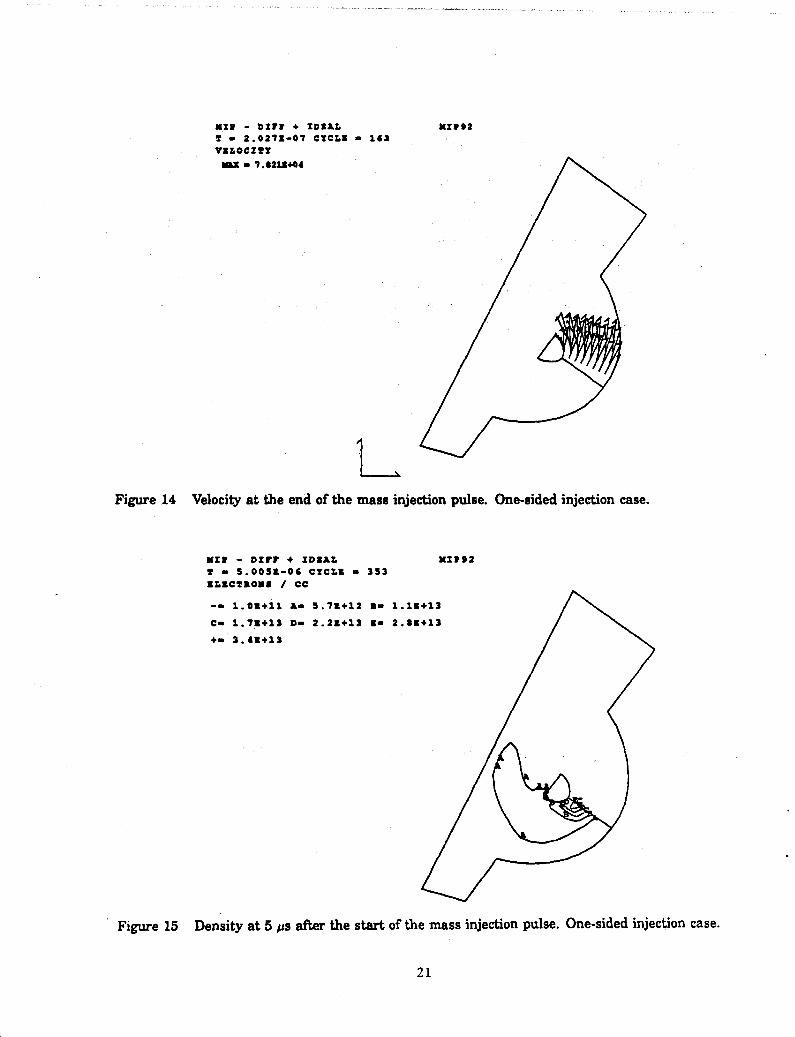
MZP - Oir» + IDSJk.L T • 2.0211-07 CTCLI - 1(3 VILOCITT
NftX - 1.121X404
MIPB2
Figure 14 Velocity at the end of the mass injection pulse. One-sided injection case.
xir - ozrr 4 IDXAX I • 5.005X-OC CTC&K - 353 KLKCTILOBI / CC
MIf92
1.0X4-11 &• S.71+12 •• 1.11+13 1.71+13 0- 2.2B+13 C- 2.•1+13 3.4K+13
Figure 15 Density at 5 ps after the start of the mass injection pulse. One-sided injection case.
21

Mif - oirr + xoxxi. T - 5.00SX-0« CXCL1 • 3S3 VII.OCITT
mix - 3.1111+04
M»12
Figure 16 Velocity at 5 /is after the start of the mass injection pulse. One-sided injection case.
Time (us)
Figure 17 Electron density vs. time at the simulation density probe locations. One-sided injection case.
22

6. Conclusions and Recommendations The simulations reported here provide a prediction of the structure and develop¬
ment of the MIP switch plasma during the plasma formation interval. The principle implication for PBFA II is that cathode density measurements may not measure the mass in the switch. The simulations seem to suggest that the total switch mass may rise much faster than the cathode density and begin to fall before the cathode density peaks. If switch mass is an important determinant of switch opening time, using cathode density diagnostics to determine plasma formation time may be misleading.
This simulation model should aid in selection of the plasma formation time for MIP POS shots. The qualitative agreement with experimentally measured plasma densities is sufficiently good that bringing the model into quantiative agreement by adjusting the unknown inflow density and velocity profile seems worthwhile. More simulations similar to these should be run with the density probe locations set the
same as those in the experiment to accomplish that.
In order to understand the effect of this plasma distribution and the embedded poloidal field on switch performance, MHD simulations of the plasma during the
accelerator power pulse should be performed. M3P POS and current toggle (CT) POS
configurations should be simulated both with and without the Hall effect. Present theoretical understanding of the switching mechanism indicates that the Hall effect
simulations may be able to produce the first good prediction ofCT POS performance. Simulation of the CT POS will require the addition of a magnetic field boundary condition to assure that the fast field coil in the cathode generates the appropriate
amount of poloidal field as a function of the toroidal field near that boundary.
23
References
[1] Michael H. Frese. MACH2: A two-dimensional magnetohydrodynamic simulation code for complex experimental configurations. Technical Report AMRC-R-874, Mission Research Corporation, 1987.
[2] Bruce V. Weber. MIP density measurements at Sandia. Technical Report 89-28, Naval Research Laboratory Plasma Technology Division, September 1989.
24

Appendix A Historian Change File to Implement Rigid Field Lanes in MACH2
v8801_________
*id mhfdif *dk velbkf
subroutine velbkf(velx,vely,velz)
c———project velocity onto vertex magnetic field
cdir$ nolist *ca common
*ca pointer cdir$ list
dimension velx(0:ip2,0:jp2) dimension vely(0:ip2,0:jp2) dimension velz(0:ip2,0:jp2)
do 100 j-^jpl do 100 i-l.ipl
bmag - bvx(i,j)**2 + bvy(i,j)**2 + bvz(i,j)**2
bdotv - bvx(i,j) * velx(i,j) % + bvy(i,j) * vely(i,j) % + bvz(i,j) * velz(i,j)
velx(i,j) - bdotv * bvx(i,j) / ( bmag + l.e-99 )
vely<i,j) - bdotv * bvy(i,j) / ( broag + l.e-99 )
velz(i,j) - bdotv * bvz{i,j) / ( bmag + l.e-99 )
100 continue
return end
*d magmovc.42 call bkhntjl(rxnbr,rx,rvolnbr,rcnbr) call bkhntjl(rynbr,ry,rvoinbr,rcnbr) call bkhntjl(rznbr,rz,rvolnbr,rcnbr)
*d magmovc.44 call bkntjsc(rbznbr,rbz,rvolnbr,rcnbr)
*id mhfcir *d circuit.14
connnon /ciradd/ vgen,vplas,vcap,currentl.oldflux,volts(20),tfire
c——-four choices: *i circuit.16
25

c——— ident«2: don't change current c—-— ident-3: solve voltage source circuit equation *i circuit.75
elseif ( ident .eq. 3 ) then
if( tfire .It. 0.0 ) tfire=t
oldflux = flux flux=0.0
do 500 Iblk-l.nblk c—————magnetic flux (btheta*area) calculated (btheta-bzn)
call setblk call cirflx(flux)
500 continue
c————calculate the plasma resistance from c————the total joule heating: i.e. de/dt-resis*current**2
resplas - 2.0*pi*(cirheat-oldcirht)/(dt*amaxl(ccrrnt**2,1.e-99)) oldcirht = cirheat
c————calculate source voltage c——-—-piecewise linear voltage profile
do 600 k=l,20 kk°k if (timxx(k).gt.(t-tfire)) go to 700
600 continue 700 alf - (timxx(kk)-(t-tfire))/(timxx(kk)-timxx(kk-l))
vgen - alf*volts(kk-l)+(l.-alf)*volt3(kk)
c————-calculate plasma voltage vplas * resplas * ccrrnt + ( flux - oldflux ) / dt
c————do differential equations vcapnew = vcap + dt * ( currenti - ccrrnt ) / capac ccrnew = ccrrnt +2.
* dt * ( vcap - vplas ) / inducl curnew - currenti + 2. * dt *
% < vgen - vcap - resisi * currenti ) / inducl
vcap ~ vcapnew ccrrnt - ccrnew currenti - curnew
*i default.15 common /ciradd/ vgen,vplas,vcap,currenti,oldflux,volts(20),tfire
*i namlst.17 common /ciradd/ vgen,vplas,vcap,currenti,oldflux,volts(20),tfire
*i ttdmped.12 common /ciradd/ vgen,vplas,vcap,currenti,oldflux,volts(20).tfire
*i default.211 tfire - -1.
26
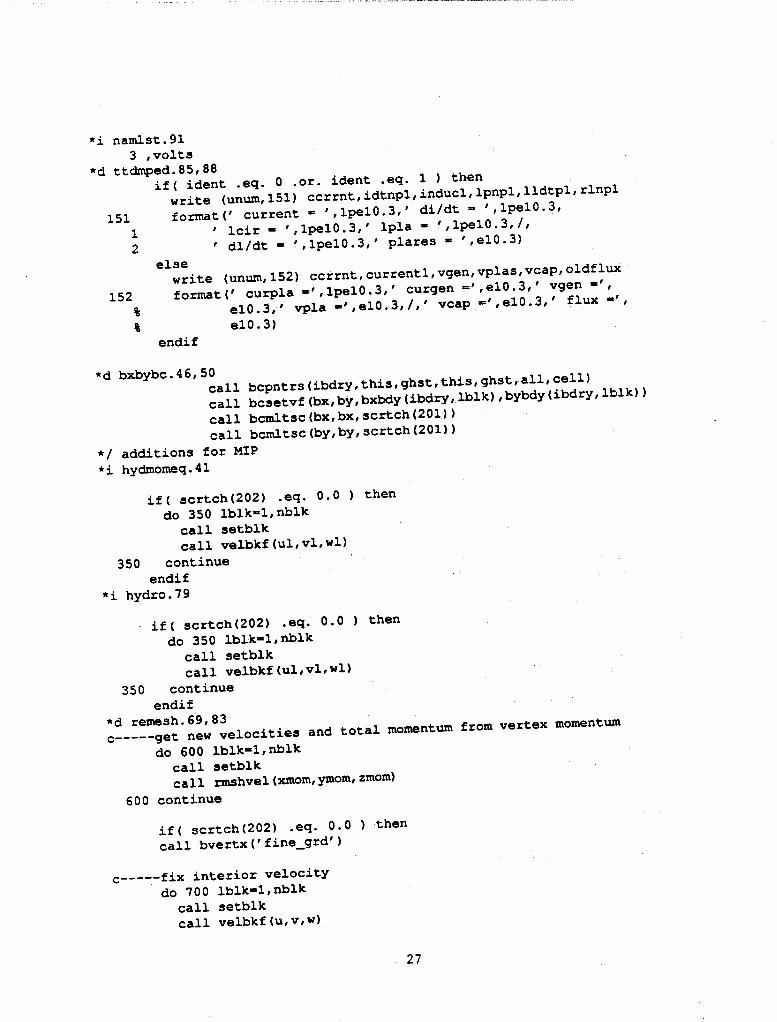
*i namlst.91 3 ,volts
*d ttdmped.85,88 if( ident .eq. 0 .or. ident .eq. 1 ) then
write (unum,151) ccrrnt,idtnpl,inducl,Ipnpl.lldtpl,rinpl 151 formatC current - ',lpel0.3,' di/dt " ',lpel0.3,
1 ' Icir - ',lpel0.3,' Ipla - ',lpel0.3,/, 2 ' dl/dt - ',lpel0.3.' plares - ',el0.3)
else write (unum,152) ccrrnt,currentl,vgen,vplas,vcap,oldflux
152 format (' curpla -',lpel0.3,' curgen =',el0.3,' vgen «', % el0.3,' vpla-',el0.3,/,' vcap-»', el0.3.' flux«', % el0.3)
endif
*d bxbybc.46,50 call bcpntrs(ibdry,this,ghst,this,ghst, all,cell) call bcsetvf(bx,by,bxbdy(ibdry,Iblk),bybdy(ibdry,Iblk)) call bcmltsc(bx,bx,scrtch(201)) call bcmltsc(by,by,scrtch(201))
*/ additions for MIP
*i hydmomeq.41
if( scrtch(202) .eq. 0.0 ) then do 350 lblk"l,nblk
call setblk call velbkf(ul.vl,wl)
350 continue endif
*i hydro.79
if( scrtch(202) .eq. 0.0 ) then do 350 lblk-l,nblk
call setblk call velbkf(ul,vl,wl)
350 continue endif
*d reroesh.69, 83
c———get new velocities and total momentum from vertex momentum
do 600 lblk-=l,nblk call setblk call rmshvel (xmom, ymom, zmom)
600 continue
if( scrtch(202) .eq. 0.0 ) then call bvertx('fine_grd')
c-——fix interior velocity do "700 lblk-l,nblk
call setblk call velbkf(u,v,w)
27

700 continue endif
c——-fix boundary velocity do 800 lblk-l,nblk
call setblk call velbcf(u,v,w)
800 continue
do 900 lblk-l,nblk call setblk
c————fix corner velocity call velccf<u,v,w)
c————get internal energy from total energy call totnrg2(conserv,rofanom,siecap,mO)
900 continue * i hydmomeq.3 4
bmult - bmult * scrtch(202) dmult - dmult * 3crtch(202)
*i hyditblk.82
sbx(i) = scrtch(202) * sbx(i) sby(i) » scrtch(202) * sby(i) sbz(i) - scrtch(202) * sbz(i)
*d hyditblk.267,269 bxl(i,j) = bxl(i,j) + scrtch(202) * dbx(i)
*d hyditblk.267,269 bxl(i,j) - bxl(i,j) + scrtch(202) * dbx(i) byl(i,j) - byl(i,j) + scrtch(202) * dby(i) bzl(i,j) - bzl(i,j) + scrtch(202) * dbz(i)
*i cournum.25 cmag " cmag * scrtch(202)
*d trnspt.62,64 a = scrtch(202) b - 1 - scrtch(202) bxn(i,j) - a * mp<i,j) * bxl(i,j) + b * bxl(i,j) byn(i,j) « a * mp(i,j) * byl(i,j) + b * byl(i,j) bzn(i,j) - a * mp(i,j) * bzl(i,j) + b * bzl(i,j)
*i trnspt.137 dbxbs - scrtch<202) * dbxbs
*i trnspt.142 dbybs - scrtch(202) * dbybs
*i trn3pt.238 dbxis - scrtch(202) * dbxis
*i trnspt.243 dbyls - 5crtch(202) * dbyls
*i trnspt.296 dbzbsp = scrtch(202) * dbzbsp dbzbsm - 3crtch(202) * dbzbsm
*i trnspt.322 dbzisp «" scrtch(202) * dbzbsp
28
dbzism - scrtch(202) * dbzbsm *d trnspt.334,336
a - scrtch(202) b - 1 - scrtch<202) bxn(i,j) - a * bxn(i,j) / mp(i,j) + b * bxn(i,j) byn(i,j) - a * byn(i,j) / nip(i,j) + b * byn(i,j) bzn(i,j) - a * bzn(i,j) / mp(i,j) + b * bzn(i,j)
*id mhfhst *dk fnne
function fnne(i,j)
c—— compute electron number density in cell i,j cdir$ nolist *ca common
*ca pointer cdir$ list
fnne - nfe(i,j) * ro(i,j) / ( awc(i,j) * pm )
return end
*i history.12 external fnne
*d history.44,45 c—————— get ne at first hstnumfc locations
histf(num) - histvalut fnne , num.)
29
Appendix B MACH2 Input File for MIP Simulation Low Density Case
MIP - diff + ideal $contrl
intty " 48htiinencyc,10;timestep, 10,'perform, 10,-enrgynow, 10; intty(7) - 40hbadcells,10;blanlc, 10; currents 10
Ipr - 1,
irons - 30, twfn - lO.Oe-6, dt - l.e-10, dto « 0.05e-6, dtrst c l.Oe-6, dtmax • l.e-9,
idealgas - .true., gml -' 0.667,
hydron - .false., omegah « 0.66, volratm « 0.9, courmax - 1.0, rmvolrrn - 0.2, mu m 5.6,
rad - 6hdirtyh ,
fox - 0.1, ciron " .false., thmldif - .false.,
fiximt - 0.04, meshon " .false.,
nsmooth = 4, wrelax -• 0.25.
brbzon - .true., magon » .true.,
itpot - 20, potrelx - 0.5,
bdiff - .true., joultmit -0., roultgrd -B .true., mgmode = Shconverge, rdtol - l.e-4, cntnnin « 1.0,
scrtch(201) ° 2.64, scrtch(202) -
0.,
nhist=5,
30

fdycupr- 1.91e-4, hstnumfc » 4, histnum = 4,
rof aresvac » 100., rofanom = 1.5e-9,
histx(l) -
histx(2) =
histx(3) °
histx(4) -
- l.e-9,
0. 0. 0. 0.
2134, 2599, 2521, 3186,
histyd) histy(2) histyd) hi3ty(2)
= 0
= 0
" 0
= 0
.2992,
.2646,
.3875,
.3407,
plot(7) » 8hdiffusiv .
$end $curnt
ident = 3, capac - 4.e-10, inducl = 100.e-9, resisi - 4.4,
tin>xx( 1)= tinucx( 6)- timxxdl)- timxx(16)-
volts(l) volts(6) '
volts (11) '
volts(16) '
$end $ezgeom
0. 0.7012e-07, 0.1168e-06, 0.1702e-06,
• O.OOe+00, • 1.07e+07. ' 4.66e+06, • -2.76e+Q6,
0.3007e-07, 0.7680e-07, 0.1435e-06, 0.1769e-06,
6.84e+04, 1.20e+07,
-1.85e+06, -1.98e+06,
0.3674e-07, 0.8348e-07. 0.1502e-06, 0.1836e-06,
1.57e+05, 1.22e+07,
-3.24e+06, 3.06e+06,
0.4342e-07, 0.9015e-07, 0.1569e-06, l.e-3,
0.5010e-07, 0.9683e-07, 0.1635e-06,
6.38e+05, 1.16e+07,
-3.80e+06, 3.06e+06,
2.23e+06, 1.06e+07,
-3.56e+06,
npnts = 20, pointxd) - 0.2914, pointyd) - 0.4757, pointx(2) - 0.3801, pointy(2) - 0.4104, pointx(3) - 0.2521, pointy(3) '• 0.3975, pointx(4) - 0.3286, pointy(4) - 0.3407, pointx(5) - 0.2132, pointy(5) - 0.3201, pointx(6) - 0.2776, pointy(6) - 0.2722, pointx(7) - 0.1980, pointy(7) - 0.2898, pointx(8) - 0.2577, pointy(8) - 0.2454, pointx(9) - 0.1590, pointy(9) - 0.2123, pointx(lO) = 0.2066, pointy(lO) = 0.1770, pointxdl) " 0.1243, pointy (11) - 0.1434, pointx(12) = 0.1713, pointy(l2) - 0.1296, pointx(13) - 0.2866. pointy(l3) = 0.2576, pointx(14) - 0.3511, pointy(14) - 0.2690,
31

pointx(15) pointx(16) pointx(17) pointx(18) pointx(19) pointx (20)
- 0
- 0
= 0
- 0
- 0
" 0
.2855
.3318
.2742
.2822
.2855
.3318
/
/
f
9
9
9
pointy pointy(16) pointy pointy pointy pointy
(15)
(17) (18) (19) (20)
= 0
° 0
= 0
- 0
» 0
- 0
.2455,
.2111,
.2410,
.1762,
.2455,
.2111,
nblk - 9, corners(1,1) " 1,2,4,3, corners(1,2) « 3,4,6,5, corners(1,3) - 4,14,13,6, corners(l,4) - 14,16,15,13, corners(1,5) « 5,6,8,7, corners(l,6) - 7,8,10,9, corners(l,7) - 8,17,18,10, corners(l,8) « 17,19,20,18, corners(1,9) - 9,10,12,11,
numarcs - 8, arctype(l) = 7h2pt&dir ,
arctype(2) «° 7h2pt&dir ,
arctype(3) ° 7h2pt&dir ,
arctype(4) » 7h2pt&dir ,
arctype(5) "- 7h2pt&dir ,
arctype(6) = 7h2pt&dir ,
arctype(7) = 7h2pt&dir ,
arctype(8) - 7h2pt&dir ,
arcsd.l) - 14,4 , 0.5080. arcs(l,2) - 14,16,-0.4920, arcs(l,3) - 13, 6, 0.5918, arcs(l,4) « 13,15,-0.4082, arcs(l,5) = 18,20, 0.0846, arcs(l,6) - 18,10.-0.9154, arcs(l,7) - 17,19, 0.0014, arcs(l,8) - 17, 8,-0.9986,
$end $ezphys
ang -2., awg "12., gdvlg -
0., roig » 2.e-9, tempig - 0.025, icellsg - 8, jcellsg - 8, matnameg » Ihc ,
etaOg - 2.5e4, atamaxg -
1., dirintpg « 7hintp3tl,
$end $inmesh
32
name (5) = 8hmip92 ,
name <6) - 8h ,
nigen - 0, niter "• 1, eqvol • 0., siecap " 3.2482ell, vfqctim = -0.05e-6,
ibcseq(l.l) - 1,3.2,4,
magxybcd.l) « Shconductr, rnagzbcd,!) m Bhinsulatr,
currcir(l,l) • 1, hydbcd,!) - Shflowthru,
roflowd.l) - l.e-9, tflowd,!) - 0.025, eflowd.l) = 9.04e5, pflowd.l) - 6.03e-4,
ibcseqd,2) - 1,3,2,4,
ibc3eqd,3) - 1,3,2,4, icells(3) - 4,
magxybc(3,3) - Shspecfied, bxbdy(3,3) - 0.5247,
r bybdy(3,3) - -0.8513,
ibcseqd.4) » 1,3,2,4, icells(4) - 4,
magxybc(3,4) •" Shspecfied, bxbdy(3,4) - -0.0905, bybdy(3,4) - -0.9959,
magxybc(2,4) " BhsyBnmetry,
potbc(2,4) - Bhtdotgphi, hydbc(2,4) - Bhflowthru. velbc(2,4) - Shpulsed,
roflow(2,4) - 5.e-7, tflow(2,4) - 1.0, e£low(2,4) - 3.62e7, pflow(2,4) - 2.41e-l, uflow(2,4) - 6.e4, vflow(2,4) - 8.e4,
jcells(5) - 4, ibcseqd.5) - 1,3,2,4,
magxybc(2,5) - Shspecfied, bxbdy(2,5) - 0.5962, bybdy(2,5) - 0.8029,
ibcseq(l,6) " 1,3,2,4,

ibc3eq(l,7) " 1,3,2,4, icells(7) - 4,
magxybc(l,7) - Bhspecfied, bxbdy(l,7) - -0.9662, bybdy(l,7) » 0.2577,
ibc3eq(l,8) - 1,3,2,4, icells(8) - 4,
magxybcd, 8) - Shspecfied, bxbdy(l,8) - -0.9290, bybdy(l,8) - -0.3700,
magxybc(2,8) - Shsynnnetry, potbc(2.8) - 8htdotgphi, hydbc(2,8) - 8hflowthru, velbc(2,8) - 6hpulsed,
roflow(2,8) - 5.e-7, tflow(2,8) - 1.0, eflow(2,8) - 3.62e7, pflow<2,8) - 2.41e-l, uflow(2,8) - -6.e4, vflow(2.8) •= -8.e4,
ibcseq(l,9) - 1,3,2,4.
magxybc(3,9) » 8hconductr, hydbc(3,9) - 8hflowthru,
ro£low(3,9) - l.e-9, tflow(3,9) •= 0.025, eflow(3,9) - 9.04e5, pflow(3,9) - 6.03e-4,
velcc(3,l) « 7hproject ,
velcc(2,2) •' 7hproject ,
velcc(3,2) *• 7hproject ,
velcc(l,3) « 7hproject ,
velcc(4,3) » 7hproject ,
velcc(2,5) - 7hproject ,
velcc(3,5) - 7hproject ,
velcc(2,6) - 7hproject ,
velcc(3,6) - 7hproject ,
velcc(l,7) - 7hproject ,
velcc(4,7) - 7hproject ,
velcc(2,9) - 7hproject ,
$end
34
$modtim
tmod = l.Oe-7,
$end $contrl
dtmax " 1., hydron « .true., counnax - 1., bdiff " .false.,
$end $modtim
tmod = 2.0e-7,
$end $contrl
dto - 0.50e-6,
$end $inmesh
velbc(2,4) - Bhfreeslip ,
probe(2.4) - 4hwall ,
velbc(2,8) - Bhfreeslip ,
probe(2,8) = 4hwall ,
Send
Distribution:
Maxwell Laboratory (3) Attn: BillRix
John Shannon Michael Coleman
8888 Balboa Avenue San Diego, CA 92123
S-Cubed (4) Attn: Andrew Wilson
Eduardo Waisman Paul Steen Don Parks
P.O. Box 1620 LaJolla,CA 92038
Naval Research Laboratory Attn: Gerry Cooperstein Code 4770 4555 Overtook Ave. SW Washington, DC 20375
Naval Research Laboratory (7) Attn: PaulOttinger
John Grossman Bob Commisso Dave Mosher Jesse Neri Bruce Weber Dave Hinshelwood (Jaycor)
Code 4771 4555 Overtook Ave. SW Washington, DC 20375
Seishi Hamasaki Jason Associates 2002 Jimmy Durante Blvd. Suite 314 Del Mar, CA 92014
Krall Associates Attn: Nick Krall 1070 America Way Del Mar, CA 92014
Lawrence Uvermore Nat. Lab Attn: Dennis Hewett MS L472
P. 0. Box 808 Uvermore, CA 94550
Los Alamos Nat. Laboratory (2) Attn: Rod Mason
Dan Winske MS E-531
P.O. Box 1663 Los Alamos, NM 87545
Comell University (3) Laboratory of Plasma Science Attn: Ravi Sudan
John Greenly Lynne Adter
369 Upson Hall
Ithaca, NY 14853
University of New Mexico (2)
Dept. of Chem. & Nuc. Eng. Attn: Norm Roderick
James Nicholson
Albuquerque, NM 87131
University of New Mexico Department of Electrical Engineering Attn: EdI Schamiloglu 323C EECE Building Albuquerque, NM 87131
Mission Research Corporation (2) Attn: JoeKindel
Erick Undman 127 Eastgate Drive, Suite 208 Los Alamos. NM 87544
Mission Research Corporation (2) Attn: BobPeteikin
Steve Payne 1720 Randolph Road, SE Albuquerque, NM 87106
Numerex Attn: MikeFrese 1400 Central SE Albuquerque, NM 87106
36
Defense Nuclear Agency RAEV Attn: Capt. Jerry Fisher 6801 Telegraph Road Alexandria, VA 22310
Berkeley Research Associates (2) Attn: Steve Brecht
Bob Kares
P. 0. Box 241
Berkeley, CA 94701
Air Force Academy Attn: Capt. Robert Lawconnell FJSRUNH Colorado Springs, CO 80840
Yale University
Dept. of Applied Physics Attn: Philippe Similon
P.O. Box 2157 Yale Station New Haven, CT 06520-2157
Roger Bengston 411 Honeycomb Ridge Austin, TX 78746
PSI Attn: lan Smith
Laslo Dimenter Kurt Neilsen
600 McCormick Street San Leandro, CA 94577
Physics International Attn: John Goyer
Peter Sincemy David Kortbawi
2700 Merced Street San Leandro, CA 94577
1200 J. P. VanDevender 1241 J. R. Freeman 1242 B.N.Turman 1260 D.LCook 1262 LP.Mix 1263 D.H.McDanlel 1263 C. W. Mendel, Jr. 1263 W. B.S.Moore 1263 G.E.Rochau 1263 M. E. Savage 1263 H.N.Woodall 1263 D.M.Zagar 1264 R.W.Stinnett 1264 T.J.Renk 1265 J.P.Qulntenz 1265 M. P. Desjarlais 1265 S. E. Rosenthal 1265 S.A.SIutz 1265 M. A. Sweeney (6) 1267 G. Cooper 1267 W.A.Stygar 1270 J.K.RIce 1271 G. 0. Allshouse 1271 T.W.Hussey 1272 G.W.Kuswa 1272 J.E. Bailey 1275 J. R. Woodworth 1290 T.H.Martin 3141 S. A. Landenberger (5) 3141-1 C. L Ward (8) for DOE/OSTI 3151 W.I.Ktein(3) 8524 J. A. Wackeny
37