Embed Size (px)
Citation preview

FRACTURE MECHANICS ANALYSIS OF
GEOMETRICALLY NONLINEAR THIN PLATES BY
FEM
HAMID TAHERI
RESEARCH PROJECT SUBMITTED IN PARTIAL
FULFILMENT OF THE REQUIREMENTS FOR THE
DEGREE OF MASTER OF PHILOSOPHY
FACULTY OF ENGINEERING
UNIVERSITY OF MALAYA
KUALA LUMPUR
2013

ii
UNIVERSITY OF MALAYA
ORIGINAL LITERARY WORK DECLARATION
Registration/Matric No: KGH100017
Name of Candidate: HAMID TAHERI
Name of Degree: MASTER OF MECHANICAL ENGINEERING
Title of Project Paper/Research Report/Dissertation/Thesis (“this Work”):
FRACTURE MECHANICS ANALYSIS OF GEOMETRICALLY NONLINEAR
THIN PLATES BY FEM
Field of Study: COMPUTATIONAL MECHANICS
I do solemnly and sincerely declare that:
1) I am the sole author/writer of this Work;
2) This Work is original;
3) Any use of any work in which copyright exists was done by way of fair dealing and for
permitted purposes and any excerpt or extract from, or reference to or reproduction of any
copyright work has been disclosed expressly and sufficiently and the title of the Work and its
authorship have been acknowledged in this Work;
4) I do not have any actual knowledge nor do I ought reasonably to know that the making of this
work constitutes an infringement of any copyright work;
5) I hereby assign all and every rights in the copyright to this Work to the University of Malaya
(“UM”), who henceforth shall be owner of the copyright in this Work and that any reproduction
or use in any form or by any means whatsoever is prohibited without the written consent of UM
having been first had and obtained;
6) I am fully aware that if in the course of making this Work I have infringed any copyright
whether intentionally or otherwise, I may be subject to legal action or any other action as may be
determined by UM.
Candidate’s Signature Date
Subscribed and solemnly declared before,
Witness’s Signature Date
Name: Designation:

iii
Abstract
In this study, general introduction and methodology of fracture mechanics analysis of
plate are developed. The geometrical nonlinearities are due to large deformation or
rotation. Two major theories in the analysis of plates consist of Kirchhoff and Reissner-
Mindlin plate theories which former is suited for thin plates and latter for thicker plates.
In order to perform geometrically nonlinear plate analysis, bending problems includes
the interaction of plate out of plane bending and in-plane loadings. Different methods
for the crack tip calculations of stress intensity factor were proposed which among them
crack tip displacement method were found to be more convenient and straight forward
for implementation based on specifically formed elements at the crack tip. During the
implementation of ANSYS®
codes, it was noticed that by applying modified Newton-
Raphson method with carefully selected numbers of iterations and sub-steps both
accuracy and time are served. Two different finite element method simulations of
geometrically nonlinear plate structures were performed. A square and a rectangular
plate possessing a center crack were subjected to different boundary conditions of
clamped and simply supported edges separately. In both examples, the range of bending
stress intensity factors was higher than the membrane stress intensity factor. By having
aspect ratios of width divided by length of the geometry, b l , upper than 1, the bending
stress intensity factor after a certain number of load increments is increasing
significantly while the membrane stress intensity factor is not having any considerable
changes for the clamped edges condition but has comparable amount for the simply
supported edges.

iv
Abstrak
Dalam kajian ini, pengenalan umum dan metodologi analisis mekanik patah plat
dibangunkan. Tak lelurus geometri adalah akibat ubah bentuk besar atau putaran. Dua
teori utama dalam analisis plat terdiri daripada Kirchhoff dan teori plat Reissner-
Mindlin yang bekas sesuai untuk plat nipis dan kedua untuk plat tebal. Dalam usaha
untuk melaksanakan analisis plat geometri linear, masalah lenturan termasuk interaksi
plat keluar pesawat membongkok dan bebanan dalam-satah. Kaedah yang berlainan
untuk pengiraan hujung retak faktor keamatan tekanan telah dicadangkan antaranya
retak hujung anjakan kaedah telah ditemui untuk menjadi lebih mudah dan lurus ke
hadapan bagi pelaksanaan yang berdasarkan unsur-unsur yang khusus terbentuk pada
hujung retak. Semasa pelaksanaan ANSYS®
kod, ia telah menyedari bahawa dengan
menggunakan diubahsuai Newton-Raphson kaedah dengan nombor yang dipilih dengan
teliti lelaran dan sub-langkah kedua-dua ketepatan dan masa dihidangkan. Dua berbeza
terhingga kaedah simulasi elemen struktur plat linear geometri telah dijalankan. A
persegi dan plat segiempat memiliki retak pusat tertakluk kepada syarat sempadan yang
berbeza daripada tepi dikapit dan hanya disokong berasingan. Dalam kedua-dua contoh,
pelbagai faktor keamatan tekanan lentur adalah lebih tinggi daripada tekanan keamatan
faktor membran. Dengan mempunyai nisbah aspek lebar dibahagikan dengan panjang
geometri, b l , atas daripada 1, tegasan lentur keamatan faktor selepas bilangan tertentu
kenaikan beban meningkat dengan ketara manakala faktor keamatan tekanan membran
tidak mempunyai apa-apa perubahan besar untuk keadaan tepi diapit tetapi mempunyai
jumlah setanding bagi tepi disokong mudah.

v
Acknowledgements
I would like to express my deep and sincere gratitude to my supervisor, Assoc. Prof. Dr.
Judha Purbolaksono for his technical advices and constructive comments throughout
this work.
I want to thank my family for their patience and encouragement, not only for my
research work, but in all dimensions of my life.

vi
Table of Contents
Abstract ................................................................................................................. iii
Abstrak .................................................................................................................. iv
Acknowledgements ................................................................................................. v
Table of Contents .................................................................................................. vi
List of Figures ..................................................................................................... viii
List of Tables .......................................................................................................... x
Chapter 1: Introduction ........................................................................................... 1
1.1 Background .......................................................................................................... 2
1.2 Objectives ............................................................................................................ 4
1.3 Types of Structural Nonlinearities ....................................................................... 5
1.3.1 Geometrical .......................................................................................................... 6
1.3.1.1 Large Deformations and Rotations .......................................................... 6
1.3.1.2 Stress Stiffening ...................................................................................... 8
1.3.2 Material ................................................................................................................. 8
Chapter 2: Literature Review ................................................................................ 10
2.1 Plate Theory ....................................................................................................... 10
2.1.1 The Basic Assumptions .......................................................................................11
2.1.2 The Kirchhoff Plate Theory .................................................................................11
2.1.2.1 Boundary Conditions ..............................................................................16
2.1.3 The Reissner-Mindlin Plate Theory ....................................................................18
2.2 Fracture Mechanics............................................................................................ 20
2.2.1 Linear Elastic Fracture Mechanics (LEFM) ........................................................21
2.2.2 Modes of Loading ................................................................................................22
2.3 Finite Element Method ...................................................................................... 24
2.3.1 Element Types .....................................................................................................25

vii
2.3.2 Advantages and Disadvantages ...........................................................................26
Chapter 3: Methodology ....................................................................................... 28
3.1 Geometrical Nonlinearity .................................................................................. 28
3.1.1 Large Displacement/Small Strain ........................................................................28
3.1.2 Solution Methods Based on Incremental-Iterative ..............................................34
3.1.2.1 Incremental Technique ...........................................................................37
3.1.2.2 Newton-Raphson Technique ..................................................................38
3.1.2.3 Modified Newton-Raphson Technique ..................................................39
3.1.2.4 Quasi-Newton Technique .......................................................................40
3.1.3 Large Displacement/Large Strain ........................................................................40
3.1.3.1 Total Lagrangian (TL) Framework ........................................................41
3.1.3.2 Updated Lagrangian (UL) Framework ...................................................41
3.2 Stress Analysis of Crack Containing Bodies ..................................................... 42
3.2.1 Singularity Elements of Crack Tip ......................................................................42
3.2.2 Solutions of Stress Intensity Factor (Ki) ..............................................................44
3.2.2.1 Displacement Correlation Approach ......................................................45
3.2.2.2 Strain Energy Release Rate (G) Approach .............................................46
3.2.2.3 Crack Tip Opening Displacement (CTOD) Approach ...........................47
3.2.2.4 J-Integral Approach ................................................................................48
Chapter 4: Results and Discussions ...................................................................... 50
4.1 Displacement Extrapolation Technique............................................................. 51
4.2 Numerically Solved problems ........................................................................... 53
4.2.1 A Center Cracked Square Plate under Transversal Loading ...............................55
4.2.1.1 Clamped Square Plate ............................................................................57
4.2.1.2 Simply-Supported Square Plate ..............................................................58
4.2.2 A Center Cracked Rectangular Plate under Transversal Loading .......................59
4.2.2.1 Clamped Rectangular Plate ....................................................................60
4.2.2.2 Simply-Supported Rectangular plate ......................................................62
Chapter 5: Conclusion .......................................................................................... 64
References ............................................................................................................. 67

viii
List of Figures
Figure 1.1 Deflections of linear and nonlinear plates while the edges are Free (a) or
Clamped (b) ...................................................................................................... 7
Figure 1.2 Nonlinearity of material ................................................................................... 9
Figure 2.1 A typical thin plate with dimensions and transverse loading system (Logan,
2011) .............................................................................................................. 11
Figure 2.2 A differential cross-section of Kirchhoff plate (Liu & Riggs, 2002) ............ 12
Figure 2.3 In-plane normal and shear stresses of a plate (Logan, 2011) ........................ 14
Figure 2.4 Twisting moments on the plate edge (Ugural & Fenster, 2003) .................... 17
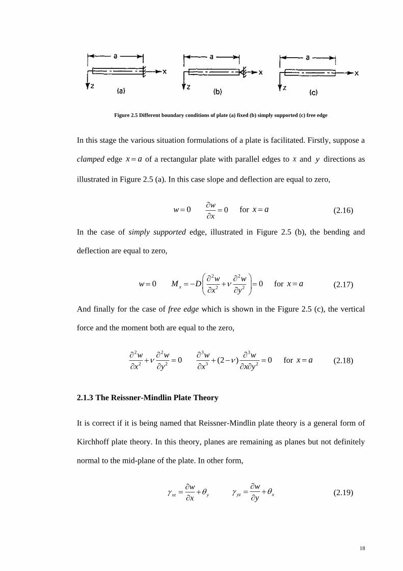
Figure 2.5 Different boundary conditions of plate (a) fixed (b) simply supported (c) free
edge ................................................................................................................ 18
Figure 2.6 A differential cross-section of Reissner-Mindlin plate (Liu & Riggs, 2002).
........................................................................................................................ 19
Figure 2.7 An arbitrary crack with fracture line and surface .......................................... 21
Figure 2.8 Fracture Modes and stresses applied on an element ahead of crack tip ........ 22
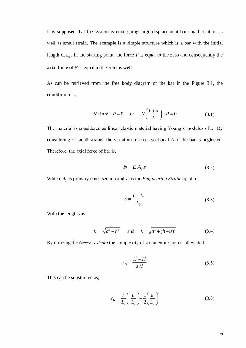
Figure 3.1 Nonlinear example of a bar ........................................................................... 28
Figure 3.2 Geometrical nonlinearity of a bar .................................................................. 31
Figure 3.3 The procedure of incremental technique ....................................................... 37
Figure 3.4 Procedure of Newton-Raphson technique ..................................................... 39
Figure 3.5 Mixed Newton-Raphson and incremental techniques ................................... 39
Figure 3.6 Modified Newton-Raphson technique ........................................................... 40
Figure 3.7 A meshed thin plate model containing edged-crack with quarter-point
elements (Bhatti, 2005) .................................................................................. 43
Figure 3.8 Stress intensity factor extrapolation (Mohammadi, 2008) ............................ 46
Figure 3.9 Crack tip opening displacement .................................................................... 47
Figure 3.10 Arbitrary contour surrounding the singularity point of crack tip (Carlson,
1978). ............................................................................................................. 48

ix
Figure 4.1 Modes of fracture for a crack in plates: (a) and (b) membrane, (c) and (e)
bending and torsion, (d) out of plane shear (Palani, Iyer, & Dattaguru, 2006)
........................................................................................................................ 51
Figure 4.2 Quadrilateral element into a triangle element transformation at the crack tip
(Anderson, 2005) ........................................................................................... 52
Figure 4.3 Formation of crack tip element with mid-points sliding to the quarter points
(Anderson, 2005) ........................................................................................... 52
Figure 4.4 Singularity elements formation at the crack tip ............................................. 55
Figure 4.5 Numerically solved problem as a plate with the clamped (a) and simply
supported (b) boundary conditions by finite element method ....................... 56
Figure 4.6 Normalized bending stress intensity factor for a center-cracked square plate
with clamped edges ........................................................................................ 57
Figure 4.7 Normalized membrane stress intensity factor for a center-cracked square
plate with clamped edges ............................................................................... 58
Figure 4.8 Normalized bending stress intensity factor for a center-cracked square plate
with simply supported edges .......................................................................... 59
Figure 4.9 Normalized membrane stress intensity factor for a center-cracked square
plate with simply supported edges ................................................................. 59
Figure 4.10 Normalized bending stress intensity factor for a center-cracked rectangular
plate with clamped edges ............................................................................... 60
Figure 4.11 Normalized membrane stress intensity factor for a center-cracked
rectangular plate with clamped edges ............................................................ 61
Figure 4.12 Normalized bending stress intensity factor for a center-cracked rectangular
plate with simply supported edges ................................................................. 62
Figure 4.13 Normalized membrane stress intensity factor for a center-cracked
rectangular plate with simply supported edges .............................................. 63

x
List of Tables
Table 3.1 Categorized methods of obtaining stress intensity factor (Nunez, 2007) ....... 44
Table 4.1 Specifications of a square plate ....................................................................... 55

1
Chapter 1: Introduction
During the uniaxial tension load of a thin plate having a crack, in the area of adjacent to
the crack the Poisson parameter will cause the transverse compression and related
stresses. And with these compressive stresses in the edges of the crack which are not
supported the local buckling is produced. The type of the applied external loads and also
the direction of the crack are affecting the intensity factor of the existing stresses. The
amount of local stresses and the change in the energy rate in the neighborhood of crack
tip is due to local bucking and consequently a geometrical nonlinear analysis is being
applied to determine them. (Barut, Madenci, Britt, & Starnes, 1997)
Linear elastic fracture mechanics (LEFM) is well-known as an effective tool for the
solution of the fracture problems for the crack-type imperfections such as the notches
and flaws within our domain as the material body which the nonlinear area of the crack
tip neighborhood is neglected (Anderson, 2005). Otherwise, for ductile materials due to
plasticity and micro imperfections, the nonlinear area of the crack-tip in comparison to
the overall domain is big enough to not being neglected (Elices, Guinea, Gómez, &
Planas, 2002).
A plate being subjected to the bending and containing imperfections in the direction of
its thickness has been debated around a decade (Datchanamourty, 2008). This is due to
complex mathematical relations for solving the three dimensional setup of the plate. As
a result imposing any simplifications is inevitable so that the problem become solvable.
In the case of a thin plate being subjected to the in-plane loading, the two dimensional

2
theory of elastic plates is a useful way for solving stress intensity factor. Whereas, for
bending of the similar structure the application of different plate theory will result to
different results. There is no exclusive argument for this fact but it is known that by
applying a simplified plate theory which includes the transverse shears and has proper
boundary conditions especially at the crack surface, the three dimensional conditions are
satisfied. For the problems of finite domains containing cracks the numerical solutions
like finite element method is advisable. By the way, applying finite element method for
solving stress intensity factors around the crack tip area is sometimes costly and
doubtful (Sosa & Eischen, 1986).
The establishment of one effective and reliable technique for the solution of nonlinear
plate analysis is an interesting topic of today’s computational mechanics research.
Fundamentally, the usage of any developed elements is based on three conditions:
appropriate performance during large deformations, eliminate locking phenomena in the
thin plates and lastly obtain better performance while working with incompressible
materials (Duarte Filho & Awruch, 2004).
1.1 Background
The first famous plates theory was named Kirchhoff thin plate theory. In this theory
which is also well-known as classical thin plate theory, it is considered that any plane
perpendicular to the neutral plane of the plate remains normal and normal as it was
before and after the deformation (Timoshenko & Woinowsky-Krieger, 1959). In this
theory the effect of shear deformations is ignored in order to allow the presentation of
the governing equations as single variable equations. This irreducible formulation
imposing second order derivatives for the strain-displacement relations and
consequently C1 continuity for the elements which means the first derivatives is also

3
continuous. Achieving the C1 continuity in between the elements is practically difficult
for two dimensional problems. Reissner and Mindlin improved the Kirchhoff plate
theory in order to account for transverse shear deformations. Their theory proposed that
the perpendicular plane to the neutral plane of the plate before deformations remain
plane but no need to remain perpendicular after the deformations. This theory is known
as moderately thick plate theory or also well-known as shear deformation theory. In this
theory the variation of the in-plane displacements are considered to be linear but the
displacement in the transverse direction is constant (Datchanamourty, 2008). This
arrangement will result in a set of equations for strain displacement which consist of no
second order derivatives for displacement. Thus, for finite element model the C0
continuity is satisfactory which means variables only possess derivatives of maximum
order one. On the other hand, applying finite element method for Reissner-Mindlin plate
theory induce other problems such as shear locking (Zienkiewicz, 1971). Shear Locking
is referred to the problem of interpolation functions of the element producing
unexpected infinite shear strains while implementing the element bending (Bower,
2009). This phenomena is mostly appears in fully integrated first order elements like
solid elements, Timoshenko elements of beam theory and Reissner-Mindlin plate
elements (Prathap, 1985). In order to alleviate this problem in analysis there are two
suggested methods. (1) Reduced integration (2) Mixed formulation (Zienkiewicz &
Taylor, 2000). Zienkiewicz (1971) introduced the reduced integration method which
with its implementation on formulations expressed by displacement the stiffness matrix
is calculated with low-ordered integrations rather than those formulations that precisely
integrating the polynomial. The separation of components of bending and shearing
expressed in the stiffness matrix are being done in prior to the numerical integration.
While integrating of those shear components, the shear stiffness coefficients are reduced
the shear locking of the thin plate. If the shear components are reduced while the

4
bending components are still fully integrated, this case is indicated as selective-reduced
integration and has been proven to have acceptable outputs in most problems
(Zienkiewicz & Taylor, 2000). The initial variables in the finite element formulations
which are based on displacement are displacement and rotation. In the case of mixed
finite element formulations, beside the displacement variables the forces variables are
interpolated separately. The fundamental of virtual work which is one effort in order to
minimum the total potential energy might be implemented to obtain equilibrium
equations of finite element formulations are based on displacement. The mixed
formulation is obtained with the application of variational method of Hellinger-Reissner
(Datchanamourty, 2008). By using this method, the total energy is defined with strain
and complimentary energies while normal and shear stresses and displacement are as
their unknowns (Datchanamourty, 2008).
One of the most important issues in engineering of solid mechanics is the geometrical
nonlinear behavior. Initially Levy dealt with bending of plates with rectangular shape
under large deformation implementing von Karman equation expressed with
trigonometric series. Berger established the large deformation analysis of a plate
resulted in Berger equation (Purbolaksono & Aliabadi, 2005).
1.2 Objectives
The structural analysis of engineering problems may have diversity in shape and
complexity. The finite element analysis of complex problems possesses accuracy in
comparison to analytical methods.
The primary objective of this study is to summarize equations of geometrically
nonlinear domain in the form of matrices which are well suited for finite element
formulations. The presented research project deals with the calculation of bending and

5
membrane stress intensity factor at the crack tip. Also this study investigate the
proposed formulations of Purbolaksono et al. (2012) for determining the bending and
membrane stress intensity factors separately as the commercial software such as
ANSYS®
only can compute the membrane stress intensity factor.
Two numerically solved examples are presented. A thin square plate and a thin
rectangular plate under increasing transversal loadings are simulated using ANSYS®
commercial software in order to study the effects of crack length variation through
comparing their results. The size effects of plate lengths are also observing by using
rectangular plate and relating to the bending and membrane stress intensity factors.
Finally, it is also aimed to find best combination of plate size and crack length in
relation to bending and membrane stress intensity factors for industrial applications.
1.3 Types of Structural Nonlinearities
The majority of physical phenomena in the world are best described with the
assumption of being nonlinear. By the way, sometimes and for some cases a problem is
being presented in the linear form in order to keep the simplicity of the system reserved.
However, in other situations linearity assumption will result in inaccurate outcome. So,
in those cases the nonlinear behavior of the system must be considered. Nonlinearity of
a physical system may occur due to geometrical or material nonlinearities in addition to
any alteration in structural integrity and the boundary condition of system (Madenci &
Guven, 2006). Geometrical nonlinearity is because of existence of any large
deformation or rotations while the material nonlinearity happens when the stress-strain
behavior of problem is nonlinear (Sathyamoorthy, 1997). The different aspect of
nonlinearities may be categorized as in below.

6
1.3.1 Geometrical
Two kinds of geometrical nonlinearity which may occur in a physical system are
defined as large deformations and rotations and stress stiffening.
1.3.1.1 Large Deformations and Rotations
The necessity of large deformations analysis might be arisen if the considered structure
facing large displacement relative to the smallest dimensional quantity. The large
rotations analysis will be demanded when the initial condition, dimension and loading
settings vary considerably. For instance, by considering one fishing rod possessing
minor lateral stiffness when exerted lateral loading faces large deformation and rotation
(Madenci & Guven, 2006).
In general plate analysis in sake of simplicity it is supposed that deflection of a plate is
small relative to its thickness (deflection 0.2 thickness). But as it may be observed
for some engineering practices such as naval and aerospace industries, the deflection of
plates is not behaving linear anymore. Thus, for including the extra nonlinear behavior
of plate in the analysis more assumptions must be considered to cover the effect of large
deflection of the plate. It is proposed that by applying deflections further than a specific
magnitude (deflection 0.3 thickness) the respond of deflection to the exerted loading
system is not linear (Szilard, 2004). Large deflections result in mid-plane stretches,
causing of in-plane forces which increase the capacity of plate to carry loads
(Figure 1.1). In this way, while a plate undergo large deflections, boundary conditions
have significant influence on the size of developed membrane forces. For a simply
supported edges setup, when constraints allow rotations but not any horizontal
displacements ( 0u v ), edges face stress-free situation perpendicular to the boundary
while tensile stress are being produced in other in-plane locations.

7
Figure 1.1 Deflections of linear and nonlinear plates while the edges are Free (a) or Clamped (b)
By moving away from the edges the magnitude of these stresses are increased. On the
other hand, different situation are being observed when the edges of a plate are fixed. It
means that nearby the clamped edges, tangential and normal stresses are being
generated at the same time which is why just in this situation fully-exerted tensile
stresses are able to take some portion of lateral loadings. The load capacity of a plate
being considerably raised when the plate is deformed more than 50% of its thickness.
For the condition in which the amount of maximum deflection is approximately equal to
the thickness of plate ( maxw h ), the membrane behavior is similar to the bending of a

8
plate. For more of this ( maxw h ) the membrane behavior is the majority. As a result,
for these sorts of plate problems, the application of large deflection formulations, that
includes the in-plane membrane force system, is compulsory. Though, in the large
deflection formulation of plates it is supposed that the magnitude of plate deflections are
as same or higher than the thickness of the plate, in comparison to other dimensions of
the plate should be kept small (Szilard, 2004).
1.3.1.2 Stress Stiffening
Stress stiffening is happening while the change of stress in one sense is able to change
the stress in the other sense. Normally this behavior is being observed when the
magnitude of stiffness in compression is not significant in comparison to the one in
tension. The examples of stress stiffening can be mentioned as cables, membranes or of
twisting structures (Madenci & Guven, 2006).
1.3.2 Material
As illustrated in Figure 1.2 the stress and strain diagram of nonlinear material is
presented. Linear material behavior is being considered if the material is approximately
linear in the stress and strain diagram until proportional limit while the stresses
produced by the loading system is not exceeding the magnitude of yield stress point in
other locations of the material.
The nonlinearity of material might be categorized as below:
Plasticity: Permanent deformations in the material which is not depending to time.
Creep: Permanent deformations in material which is depending to time.

9
Nonlinear Elastic: Nonlinear stress-strain diagram that while removing the loadings the
material will return to its initial condition without having any permanent deformations.
Viscoelasticity: While having constant loading system the deformations are depending
to time. When removing the loadings the material will return to its initial condition
without any permanent deformations.
Hyper-elasticity: The materials such as rubbers (Madenci & Guven, 2006).
Figure 1.2 Nonlinearity of material

10
Chapter 2: Literature Review
2.1 Plate Theory
Plates have been analyzed since 1800s. The solution of free vibrations of the flat plate
has done by Euler using mathematical expressions (Timoshenko & Goodier, 1969).
Chladni discovered different modes of free vibrations. Navier is known as the frontier of
developing modern theory of elasticity. His efforts were on the solution of numerous
plate problems and also deriving the exact differential equations of plates with
rectangular geometry having flexural resistance. He has introduced the solutions of
some boundary value problems with exact methods that substitute the differential
equations to the algebraic equivalent equations. For the solutions of lateral vibration of
different geometries such as circular plate Poisson in 1820s used and developed the
plate theory. The extended formulations of plate theory have been done by the work of
other researchers. Kirchhoff is well-known of the one who started the work on extended
plate theory. Although the implementation of finite element method which is the
fundamental of all complex structures analysis begun in 1900s, however they are being
carried out today by using user defined or commercial which they require high
performance capability to solve the problems. The statics and dynamics of plate theory
of various other shapes and forms were developed by using advanced finite element
methods.

11
2.1.1 The Basic Assumptions
At the beginning of plate bending it is demanded to express some assumptions to help in
moving forward through the formulations. Consider a thin plate which is in the x-y
plane having the thickness of t in the z-direction as depicted in Figure 2.1. The plate has
the mid-surface located at 0z and two parallel plate surfaces are positioned on its
above and below as / 2z t . In the geometry of plate is considered that: (1) the plate
has a very small thickness in comparison to other dimensions (2) the deflection of the
plate is much smaller than the plate thickness.
Figure 2.1 A typical thin plate with dimensions and transverse loading system (Logan, 2011)
2.1.2 The Kirchhoff Plate Theory
The considerations of classical thin plate theory or classical Kirchhoff plate bending
theory are much in resemblance to the assumptions of Euler-Bernoulli beam theory
(Logan, 2011). As it is illustrated in Figure 2.2, suppose a differential cross-sectional of
plate while the cutting plane is orthogonal to the x axis. The q loading will makes the
plate to experience lateral deformation or as it can be expressed in the z-direction which
the w deflection at point P is the function of x and y i.e., ( , )w w x y and the plate does
not have z-direction stretching.

12
Figure 2.2 A differential cross-section of Kirchhoff plate (Liu & Riggs, 2002)
The normal line to the plate surface that initially connecting two points of a and b will
be normal after exerting the loadings. The conditions mentioned in below are containing
the Kirchhoff’s assumptions:
1. Normal is remaining normal: Which means that 0xz and 0yz while 0xy .
Perpendicular angles in plate plane will not be perpendicular angles after
exerting loadings. Generally the plate can experience in-plane twisting.
2. By having 0z it is implied that the thickness variation may be ignored and
normal will not having any stretching.
3. The effect of normal stress z on in-plane strains of x and y of stress-strain
diagram is not significant.
4. The plate is considered to be flat at the beginning. So, at mid-surface of the plate
the deflections in the x and y directions are supposed to be zero , ,0 0u x y
and , ,0 0v x y .
5. The material is the characteristic of being elastic, homogenous and isotropic.

13
Based on these considerations the plate problem in three-dimension is being reduced to
the two-dimension plate problem. Therefore, the plate theory equations are simplified.
By having the thin plate theory assumptions as mentioned in above the mathematical
formulation one is being derived. In the following the Kirchhoff’s plate theory
formulation in Cartesian coordinates are considered.
According to the Kirchhoff theory assumptions any arbitrary point P in the depicted
plate of Figure 2.2 has x component displacement which is because of small rotation of
y .
,y x
ww
x
,x y
ww
y
(2.1)
In a same way but in the y-direction,
( )y
wu z z
x
( )
wv z
y
(2.2)
The plate’s curvature are then expressed as the rate change of angular displacements of
the normal which are,
2
2x
w
x
2
2y
w
y
22xy
w
x y
(2.3)
And accordingly the in-plane strains are,
2
2x
wz
x
2
2y
wz
y
2
2xy
wz
x y
(2.4)
Or might be derived as,
x xz x yz
xy xyz (2.5)
The first expression of above equations is being used in the beam theory. The other
pairs are for plate theory (Logan, 2011). Also, the transverse shear strains of xz and
yz in the Kirchhoff plate theory are equal to zero.

14
According to the third consideration of Kirchhoff assumptions, for an isotropic material
the in-plane stresses are related to the in-plane strains as,
2( )
1x x y
E
2( )
1y y x
E
xy xyG
(2.6)
Which 2(1 )
EG
The in-plane normal and shear stresses acting on a plate edges are illustrated in the
Figure 2.3.
Figure 2.3 In-plane normal and shear stresses of a plate (Logan, 2011)
In a same manner as beams, the stress variation in the edges of the plate is linear from
the mid-surface. Although the transversal shear stressesyz and xz shown in the
Figure 2.3 are neglected in sake of simplicity. Their stress variations through the
thickness are quadratic. The acting bending moments on the edges are related to the
stresses by,
/2
/2
t
x xt
M z dz
/2
/2
t
y yt
M z dz
/2
/2
t
xy xyt
M z dz
(2.7)
Or in the matrix form as (Ventsel & Krauthammer, 2001),

15
/2
/2
x xt
y y
t
xy xy
M
M zdz
M
(2.8)
For strains it is simply needed to substitute stresses in the bending moment’s equations
which by using curvatures for strains it becomes (Ugural & Fenster, 2003),
( )x x yM D ( )y y xM D (1 )
2xy xy
DM
(2.9)
Where 3
212(1 )
EtD
is Flexural Rigidity (Cook, 2001; Ventsel & Krauthammer, 2001)
or plate Bending Rigidity (Logan, 2011).
The plate bending equilibrium equations are vital due to demand for selecting the
displacement fields. These equations which are governing are,
0yx
QQq
x y
0xyx
x
MMQ
x y
0y xy
y
M MQ
y x
(2.10)
Which q is the transverse distributed loading and transverse shear forces are xQ and yQ
as are depicted in the Figure 2.3 (b).
By substituting the equivalent expressions of moments and curvatures in the above
equations and solving xQ and yQ which later will be replaced in the first expression of
the above equation, the partial differential equation of an isotropic plate bending may be
derived as below,
4 4 4
4 2 2 4
2w w wD q
x x y y
(2.11)
Or by introducing bi-harmonic operator (Ventsel & Krauthammer, 2001) as,

16
4 4 4
4
4 2 2 4
2
x x y y
(2.12)
Results in more simple form of
2 2 4( )
qw w
D (2.13)
The resulting answer of plate bending formulation is relative to the transverse
displacement of w. By neglecting the terms in the y-direction for one-dimensional
problems the above equation will be simplified to the beam theory formulation and the
flexural rigidity of the plate replaces to the EI of the beam theory while the Poisson
ratio is being set to zero (Wang, Reddy, & Lee, 2000).
2.1.2.1 Boundary Conditions
Two various boundary conditions need to be fulfilled in order to solve the plate theory
formulations. These pair might be slope and deflection, force and moment or any
combination of them. The main difference of the boundary conditions of beam theory
and plate theory consist in resultant of twisting moments along the plate edge. The
convenient corresponding vertical forces then have to be substitute with those moments
and later joined with shear forces in order to outcome one effective vertical force
(Ugural & Fenster, 2003). Suppose on plate having two neighboring elements with
length dy on the x a edge of the plate as illustrated in the Figure 2.4. The right hand
side element is subjected to the moment of xyM dy while on the left hand side element
the twisting moment of ( / )xy xyM M y dy dy acting.

17
Figure 2.4 Twisting moments on the plate edge (Ugural & Fenster, 2003)
From the Figure 2.4 (b) it is obvious that the aforementioned moments have been
substitute with the equivalent force coupling which results in local variation of stress
distribution for edge x a . This replacement will only affect the mentioned edge and
other edges are remaining same. On the left edge of right hand side element the upward
force of xyM is acting and the right edge of left hand side element is subjected to the
downward force of ( / )xy xyM M y dy . The resultant of these forces which are per unit
length, /xyM y , may be added to the transverse shearing force of xQ in order to
create one effective transverse edging force of xV known as Kirchhoff’s force (Ugural &
Fenster, 2003) which is shown in Figure 2.4 (c).
xy
x x
MV Q
y
(2.14)
Or after substitution in the differential equation of plate it becomes,
3 3
3 2(2 )x
w wV D
x x y
(2.15)
18
Figure 2.5 Different boundary conditions of plate (a) fixed (b) simply supported (c) free edge
In this stage the various situation formulations of a plate is facilitated. Firstly, suppose a
clamped edge x a of a rectangular plate with parallel edges to x and y directions as
illustrated in Figure 2.5 (a). In this case slope and deflection are equal to zero,
0w 0w
x
for x a (2.16)
In the case of simply supported edge, illustrated in Figure 2.5 (b), the bending and
deflection are equal to zero,
0w 2 2
2 20x
w wM D
x y
for x a (2.17)
And finally for the case of free edge which is shown in the Figure 2.5 (c), the vertical
force and the moment both are equal to the zero,
2 2
2 20
w w
x y
3 3
3 2(2 ) 0
w w
x x y
for x a (2.18)
2.1.3 The Reissner-Mindlin Plate Theory
It is correct if it is being named that Reissner-Mindlin plate theory is a general form of
Kirchhoff plate theory. In this theory, planes are remaining as planes but not definitely
normal to the mid-plane of the plate. In other form,
xz y
w
x
yz x
w
y
(2.19)

19
where x and y are relative rotations of the line with respect to normal of the mid-
plane during the undeformed condition of plate. Accordingly, the displacements are as,
yu z xv z ( , , ) ( , )w x y z w x y (2.20)
which are illustrated in Figure 2.6.
Figure 2.6 A differential cross-section of Reissner-Mindlin plate (Liu & Riggs, 2002).
From Equation (2.20) the in-plane strains and curvature of the plate bending are as
Equation (2.4) and Equation (2.3), respectively. Based on Reissner-Mindlin
assumptions the transverse shear strains are not equal to zero anymore and their value
can be obtained y,
xz y
w
x
yz x
w
y
(2.21)
The bending moments equations of Reissner-Mindlin formulation is same as the
corresponding one for the Kirchhoff plate Equation (2.9). But due to existence of
transverse shear strains of Equation (2.21) the transverse shear forces of xQ and yQ are
measured with the equations of,

20
2
1 0
0 1
x xz
y yz
QGk t
Q
(2.22)
which 2k is the shear correction factor and the magnitude of 5
6 is considered for the
case of irregular shear distribution (Liu & Riggs, 2002).
2.2 Fracture Mechanics
In 1900s, the principals of fracture mechanics was developed (Perez, 2004) which the
experimental results accompanied with the theory of elasticity helped to develop
different area of studies of fracture mechanics. The difference between the theoretical
results and those ones of experimental observations of a brittle material specimen under
tensile test was assigned to the existence of different forms and sizes of imperfections
such as tiny flaws and defects which made significant changes in the stress distribution
around the flaws without considering their true sizes. The way a crack has been
analyzed was changed after introducing the concepts in the fracture mechanics like
stress intensity factor and energy release rate. Based on theoretical analyses, the stress
concentration of up to 3 was predictable for the case of an even tiny circular hole
neighborhood within the body of a large enough plate under tension. The solution of
classical problems was introduced after the development of general energy rate methods.
This method in the classical fracture mechanics allowed for solving the nonlinear
problems. The J integral was a great hit that introduced strong numerical method and as
efficient as finite element methods for solving required fields. Further developments
were introduced after conjunction of classical principals of fracture mechanics for crack
stability criterion and analytical methods of finite element method in order to let the
simulations of different geometries, loads and boundary conditions (Mohammadi, 2008).

21
2.2.1 Linear Elastic Fracture Mechanics (LEFM)
The behavior of linear elastic material assumption is being applied for the analysis of
the isotropic, homogeneous materials while the stress field around the crack tip is
considered (Reuter, Underwood, & Newman, 1995). In this method the dimensions of
the plastic area nearby the crack tip is assumed to be small in comparison to the overall
dimension of the body and also the crack itself. The virtual roll of this assumption, so-
called small-scale yielding (Reuter et al., 1995), will result in facilitated stress field
analysis in the neighborhood of the crack tip.
Assume the fracture surface of arbitrary crack shown in Figure 2.7. A local coordinate
system might be defined at any location of the crack front with 1x , 2x and 3x as
perpendicular to the crack front, perpendicular to the crack surface and tangential to the
crack front respectively. In the 1 2x x plane the polar coordinate system of ( , )r can be
defined. From the view point of an observer, moving close to the crack line front and
along any path as is the x3 constant in the direction of the crack tip, the crack front line
would be look like a straight line and the crack surface as a flat surface. With these
conditions in hand, one three dimensional problem would simplified to a two
dimensional problem. The external loads and the problem geometry will be sensed just
from the direction and magnitude of stress at the area of the crack tip.
Figure 2.7 An arbitrary crack with fracture line and surface

22
2.2.2 Modes of Loading
Base on the crack surface displacements, a body containing a crack may have three
kinds of loadings. The mechanical response of a domain with a particular size and
geometry can be determined with stress intensity factors (Perez, 2004). The three
components of stress field at the crack tip, Mode I, Mode II and Mode III, are depicted
in Figure 2.8 (a).
With the crack growing in the direction of the crack plane and perpendicular in the
sense of the loadings, stress intensity factors may be determined based on ASTM E399
as,
0
lim 2 2I yy I yyr
K r f r
which , 0yy yy r (2.23)
Figure 2.8 Fracture Modes and stresses applied on an element ahead of crack tip

23
0
lim 2 2II xy II xyr
K r f r
which , 0xy xy r (2.24)
0
lim 2 2II xy II xyr
K r f r
which , 0xy xy r (2.25)
Which ( )If , ( )IIf and ( )IIIf are functions with trigonometric terms that are
derived analytically (Perez, 2004).
Hence, bodies containing any imperfections such as cracks or flaws can undergo
different loadings base on the stress intensity factor for a specific mode depicted in
Figure 2.8. Then, this will be similar to the perfect body loaded with the stress of . The
coordinate system of r and are defined at the plastic zone of the crack tip. With the
0 in the Figure 2.8, the stress field is in plane and along with the crack.
The stress intensity factor is the function of three parameters of stress, geometry of the
crack and the configuration of specimen (Perez, 2004) and can be shown as iK with i =I,
II, III for modes 1, 2 and 3, respectively. The parameter iK allows for the computation
of stress in fracture, crack growth rate in fatigue and crack growth rate in corrosion as
well. In the case of elastic materials, iG (strain energy release rate or known as crack
driving force) is directly proportional to the stress intensity factor and reversely
proportional to the modulus of elasticity as shown in the relationship below (Broberg,
1999).
2
ii
KG
E
(2.26)
Which
E E for plane stress (MPa)
2/ (1 )E E for plane strain (MPa)

24
E Elastic modulus of elasticity (MPa)
Poisson’s ratio
The equation in above is a basic mathematical model for fracture mechanics and
particularly for mode I of fracture.
2.3 Finite Element Method
In early 1940s and firstly in order to analyze different components existing in the
aircraft industry, the finite element method introduced and over decades it became the
most desirable method among other computational methods which benefit engineers and
scientists in the variety of areas. From the viewpoint of complicity, the analytical
solutions of everyday problems such as determining the stress field in structural
mechanics is cumbersome or for the most of engineering problems it is extremely
tedious. As the result, the retrieved solutions for the engineering problems by
introducing and implementing the numerical methods have been approximate but
mostly acceptable. By utilizing the powerful computers the way for analyzing most of
the solid structures with complex shapes and difficult boundary conditions in the era of
practical engineering has been facilitated. With the fundamental principal of finite
element method which is discretization, the structure breaks down to limited number of
elements that these elements are connected to each other with the so called nodes. Any
material properties and governing equations are defined over the elements and
expressed at nodes in terms of nodal displacement. During assembling of the elements
within the body the loads and constraints are resulting in some governing equations that
these equations are derived by applying a proper variation principle. The response of the
structure is given by solving these equations. The accuracy of the results from
implemented finite element method is merely related to various parameters like

25
selection of proper element type, selection of the enough large number of elements or
using higher-order elements. With the existence of strong and modern computers
accompanied with the developments in the era of numerical methods, design and
optimization of different statics and dynamics structures or phenomena become much
more facilitated (Desai, 2011).
2.3.1 Element Types
As might be seen in various commercial simulating programs, the different kinds of
elements are as below:
TRUSS element: Any long and thin element with this condition that its length is very
long with respect to its area while just supporting tensile or compressive loadings in the
longitudinal direction.
BEAM element: Any long and thin element with this condition that its length is very
long with respect to its cross-wide while able to support lateral loadings that make
bending.
TORSION element: Similar to the truss element whereas just supporting torsional
loadings.
2D SOLID element: Any element which its both geometry and loadings are in a specific
plane. With the plane stress definition it means a structure with thin thickness with
respect to the defined dimension in the plane. So, any related stresses in the cross
sectional dimension will be neglected. In the other hand, with the plane strain definition
it means a structure having largely enough cross sectional with respect to the in plane
dimensions. So, any related strain in the out plane dimension with be neglected.

26
PLATE element: Any element located in a specific plane while the loadings are out of
that plane that will result in bending while the thickness in small compared to the other
in plane dimensions. The only difference between the stress fields of plate with the
plane stress is in thickness diversity of tension – compression.
SHELL element: While it is mostly has same characteristic to a plate element, however
usually it is applied to surfaces with curvature. This type of elements are able be loaded
in plane or out of plane.
2.3.2 Advantages and Disadvantages
Finite element method is a strong, multi-purpose tool for solving variety of scientific
and engineering problems due to its organized principals (Desai, 2011). These
characters will let programmers to build fully or partly general-task software which are
applicable to different problems with no or less modifications. Finite element method
has the ability to be explained as physical expressions or robust mathematical
fundamental. Therefore, implementation of FEM on any problems will be facilitated by
understanding underneath basics of the problem’s physics while the accuracy of results
will be guaranteed by applying convenient mathematical expressions. The domain
containing more than two materials can be easily handled by giving different group of
elements different material properties. Moreover, assigning variety to properties inside
one particular element is possible by defining proper polynomial. Finite element method
can be dealt with complicated geometries easily and is able to cope with nonlinear or
dynamics phenomena. While boundary conditions will be just defined on the whole
structure rather than all elements individually, there will be no requirements for in-
element boundary condition considerations. Therefore, because of defining the
boundary conditions NOT in each finite element equations, with any change in

27
boundary conditions the field variable still will be CONSTANT (Desai, 2011). Finite
element method has the ability of dealing with multi-dimensional, continuous domain.
So, separate interpolation procedure for having the estimated solution for every node in
the domain is not demanded. FEM does not have any need for trial pre-solutions which
require to be implemented for the complete multi-dimensional domain. The more
realistic results of the solution need more accuracy in the properties of assign material.
The deficiency of finite element method is that the solution is sensitive to defined
element properties such as type, form, direction, number and size. When FEM is
implemented on computers, comparatively large amount of memory as well as time is
taken. After all, the result of solution is accompanied with other data which detecting
and separating of needed results from other is troublesome.

28
Chapter 3: Methodology
3.1 Geometrical Nonlinearity
Geometrical nonlinearities can be occurred due to existence of large strain, finite
displacements of small strains, finite rotations of small strains and instability in the
structures. For large strains can happen during the deformations of rubber or rubber like
material and also during the process of metal forming. The large displacements and/or
rotations of a structure may occur in slender structures like bar or thin plates. Structures
possessing pre-stressed conditions at the beginning can become unstable due to the
bulking.
3.1.1 Large Displacement/Small Strain
The examination of geometrically nonlinearity of a system and its characteristics are
introduced in the Figure 3.1.
Figure 3.1 Nonlinear example of a bar
29
It is supposed that the system is undergoing large displacement but small rotation as
well as small strain. The example is a simple structure which is a bar with the initial
length of 0L . In the starting point, the force P is equal to the zero and consequently the
axial force of N is equal to the zero as well.
As can be retrieved from the free body diagram of the bar in the Figure 3.1, the
equilibrium is,
sin 0N P or 0h u
N PL
(3.1)
The material is considered as linear elastic material having Young’s modulus of E . By
considering of small strains, the variation of cross sectional A of the bar is neglected.
Therefore, the axial force of bar is,
0N E A (3.2)
Which 0A is primary cross-section and is the Engineering Strain equal to,
0
0
L L
L
(3.3)
With the lengths as,
2 2
0L a h and 2 2( )L a h u (3.4)
By utilizing the Green’s strain the complexity of strain expression is alleviated.
2 2
0
2
02G
L L
L
(3.5)
This can be substituted as,
2
0 0 0
1
2G
h u u
L L L
(3.6)

30
As the strain might be chosen arbitrary the introduction of new strain has no conflict in
the process as long as the strain is not depending to the coordinate system and not
sensitive to the movement of the rigid body. Equations of (3.3) and (3.5) result in,
2 2
0 0 0
2
0 0 0
0 0
0 0
0 0
0 0
2 2
1 11 1
2 2
21
2
G
L L L L L L
L L L
L L L L
L L
L L L
L L
(3.7)
Or simply as,
21
2G (3.8)
That is altering the Hook’s law,
0
21
2
11
2
G
G
G
G
NE E
A
E
E
(3.9)
It implies that the * 11
2E E
must be used. This complexity might be ignored
due to this fact that the difference between engineering strain and Green’s strain is being
used for small engineering strains. For instance, by considering 0.002 , the G value
will be 0.002002G that the deviation is around 0.1%. For small strain condition, the
Hook’s law might be written as GE and therefore based on Equation (3.6),

31
20
2
0
1
2
E AN hu u
L
(3.10)
By replacing above expression to the Equation (3.1) and considering the small strain as
0L L , the other form of equilibrium equation will be as,
3 2 20
3
0
3 22
E Au hu h u P
L (3.11)
It is clear that the above equation is nonlinear as a function of u. From the other
viewpoint, it means that load P and displacement u are related by a curve and not a
straight line which the arrangement variations are ignored. Shown in Figure 3.2 is the
nonlinear feature of 52.1 10E MPa, 0A 100 mm2, a 200 mm and h 20 mm,
Figure 3.2 Geometrical nonlinearity of a bar
Retrieving the equilibrium equation can be implemented by using the principle of
virtual displacement. With using this method on the equilibrium state of a structure the
virtual works produced by forces internally and externally will be equal to the
applicable kinematics of virtual displacements. For the considered case of a bar in hand
the only virtual displacement is u and suits the relation in below as,

32
G
V
dV P u (3.12)
Which virtual strain G is equivalent to the virtual displacement of u . For the virtual
strain the Equation (3.6) is being utilized,
2
0 0 0
2
0
1
2
GG
du
du
d h u uu
du L L L
h uu
L
(3.13)
Due to this assumption that the virtual displacement has a very small amount, therefore
the stress magnitude will be constant. It should be mentioned that because of small
strain the volume through the body will remain unchanged; 0 0 0V V A L . So the
Equation (3.12) will be as,
02
0 0
N h uAL u P u
A L
(3.14)
And therefore,
0
h uN P
L
(3.15)
The above equation is same as the equilibrium Equation (3.1) when the relation of N
from Equation (3.10) being replaced in the Equation (3.11).
When dealing with complex geometries it is more convenient to utilize the principle of
virtual work in order to produce the equilibrium equation.
By utilizing the finite element method, displacement field is interpolated inside the
elements,

33
i i
i
u N u i i
i
v N v (3.16)
Which iu and iv are nodal displacement and iN are shape function. By substitution, the
Green’s strain has the matrix form of,
1
( )2
L N ε B B d (3.17)
With ε having the components as,
x
y
z
xy
xz
yz
ε (3.18)
In this configuration d is nodal displacement matrix. The matrix LB contains the small
displacement components and NB matrix implies that the Green’s strain is nonlinear
relative to the displacements. The equivalent virtual strains to the virtual nodal
displacement of d can be expressed as,
( )L N ε B B d B d (3.19)
Based on virtual displacement method, the internal forces produce virtual work that has
same value of virtual work done by external forces. This consideration is displayed in
the integral form of,
T T
V
dV ε σ d F (3.20)
In above F is indicating nodal force matrix.
By assuming that components of stress/strain matrices are linear relative to each other,
they can satisfy the equation of,

34
σ Dε (3.21)
That D is showing the constants of elastic material matrix.
By inserting Equation (3.19) into (3.20) results in,
T T
V
dV T
d B σ d F (3.22)
For any applicable virtual displacements of d ,
V
dV TB σ F (3.23)
Equation (3.23) states the algebraically nonlinear equations as a function of nodal
displacements d,
( ) R d F (3.24)
3.1.2 Solution Methods Based on Incremental-Iterative
As displayed in the example of a simple bar, the large displacements result in a set of
nonlinear equilibrium equations as expressed in (3.1) or (3.11). Mostly when dealing
with practical problems and utilizing finite element method, nonlinear equations as of
(3.24) appears in the formulations.
By assuming again the previous simple bar case, the equilibrium equations in (3.1) or
(3.11) might be rewritten as,
( )R u P (3.25)
Which
0
3 2 2
3
0
( )
3 22
h uR u N
L
E Au hu h u
L
(3.26)

35
Equation (3.26) shows the internal force component.
The primary step in solving the above nonlinear equation is approximating the minute
incremental forces and displacements linearly.
Presume for specified loading P it is demanded to obtain, experimentally, the
displacement u from Equation (3.25). A linear function might be utilized to determine
internal force of ( )R u du due to external force P dP and corresponding
displacementu du .
( ) ( )u
dRR u du R u du
du
(3.27)
And related equilibrium equation as,
( )u
dRR u du P dP
du
(3.28)
While Equation (3.25) is giving,
u
dRdu dP
du
(3.29)
Or
( )TK u du dP (3.30)
Which
T
u
dRK
du
(3.31)
is called the tangent stiffness. For the simple bar of aforementioned example,
0 0
T
d u h u h dNK N
du L L du
(3.32)
And by utilizing Equation (3.10) results in,

36
0 0
dN EA u h
du L L
(3.33)
Which,
0T uK K K K (3.34)
That,
2
0
0 0
E A hK
L L
is linear stiffness;
22
0 0
2u
E A u u hK
L h h L
is initial displacement
stiffness and 0
NK
L is initial stress stiffness.
The linear stiffness is not depending on displacement field that is resemblance to the
small displacement of structural analysis field. The initial displacement indicates the
influence of displacement on the stiffness. The initial stress stiffness shows the
existence of an axial load before executing incremental loading.
By combining two equations of (3.23) and (3.24) it is result in,
( d ) ( ) dT R d d R d K d (3.35)
And also
d dT K d F (3.36)
Which
T
RK
d (3.37)
is called the tangent stiffness matrix. And in a similar manner,
0T u K K K K (3.38)
In the Equation (3.38), TK is linear stiffness matrix, uK is initial displacement stiffness
matrix and K is initial stress stiffness matrix.

37
In order to solve the nonlinear Equation (3.24) it is vital to utilize the principle of
tangent stiffness matrix. In following common methods of solving are represented.
3.1.2.1 Incremental Technique
In this technique the loading is segmented into moment increments of iF . The
displacements incremental id are measured by applying a system of simultaneously
linear equations.
( 1)T i i i K d F (3.39)
With the updating criterion of,
1i i i d d d (3.40)
As the technique is illustrated in Figure 3.3, it is clear that the solution of this technique
is not accurate due to accumulated error.
Figure 3.3 The procedure of incremental technique

38
3.1.2.2 Newton-Raphson Technique
By assuming the known value of 0d , the initial prediction of nodal displacements for
loading system of F is being obtained by using linear algebraic equations of,
(0) 1T K d F (3.41)
Which (0) 0( )T TK K d is tangent stiffness matrix being used for initial displacements
calculation. Because of 1d being inaccurate, the equilibrium condition is not applicable
that implies the existence of residual nodal forces as,
1 1( ) r R d F (3.42)
Implementation of new tangential stiffness matrix of the form 1( )TK K d
accompanied with new system of linear algebraic equations results in,
(1) 1 1T K d r (3.43)
The optimized solution will be as,
2 1 1 d d d (3.44)
In the case of 2 2( ) r R d F 0 , the iteration will be proceed until adequate outcome
retrieved. Illustrated in Figure 3.4 is the iteration procedure of Newton-Raphson
technique that sometimes has mixed with incremental method as shown in Figure 3.5.

39
Figure 3.4 Procedure of Newton-Raphson technique
Figure 3.5 Mixed Newton-Raphson and incremental techniques
3.1.2.3 Modified Newton-Raphson Technique
Although Newton-Raphson technique is convenient for many practical problems, but
solving the linear equations of (3.43) is awkward for complex systems. The difference

40
between Modified Newton-Raphson technique and conventional Newton-Raphson
technique is that the former sometimes is just updating.
Figure 3.6 Modified Newton-Raphson technique
As indicated in Figure 3.6, the tangential stiffness matrix has initially being created and
separated while being used in the iterative process. Due to at once performance of
tangent stiffness matrix for the incremental loading, this technique is behaving faster.
However, the iterating process is repeating more.
3.1.2.4 Quasi-Newton Technique
There are various solving techniques for nonlinear algebraic equations known as Quasi-
Newton techniques, which the well-known one is Broyden-Fletcher-Goldfarb-Shanno
technique (BFGS).
3.1.3 Large Displacement/Large Strain
When encountering the large strain situations, it is inconvenient to ignore the structure’s
shape and volume variations. For instance, in the case of a simple bar, instead of 0A and

41
0L the current cross section A and current length L, respectively must be implemented
in the equations of (3.10) and (3.10).
Therefore, the Equation (3.20) implies that the virtual displacement method must be
applied for current volume. This configuration is also has difficulty as the current
volume is an unknown depending on another unknown yet which is displacement. Two
applicable methods for solving this problem are represented in below that facilitate the
integrals over volume.
3.1.3.1 Total Lagrangian (TL) Framework
In this configuration, integrating process is being performed on undeformed condition at
the beginning.
0
T T
G P
V
dV ε σ d F (3.45)
That 0V indicates the initial volume. Because of transforming process a stress known as
Piola-Kirchhoff stress, Pσ , must be accompanied with Green’s strain of Gε .
3.1.3.2 Updated Lagrangian (UL) Framework
This setup allows for continuous solution updating of ( 1)i while i is considered as
beginning value.
1
1
i
iT i T
A C
V
dV
ε σ d F (3.46)
In Equation (3.46), the term Cσ is for Cauchy stress tensor and Aε is Almansi strain
tensor.
42
The implementation of Total Lagrangian and Updated Lagrangian frameworks for
calculation of stress and strain demands constant virtual work done by internal forces
despite of the volume over which the integration is taken.
3.2 Stress Analysis of Crack Containing Bodies
3.2.1 Singularity Elements of Crack Tip
In theory, any situation in which results in infinite stress will produce singularity. The
reasons for this behavior may be as considering a corner instead of a fillet in order to
simplify the geometric or in the modeling, a loading system exerted on a minute area.
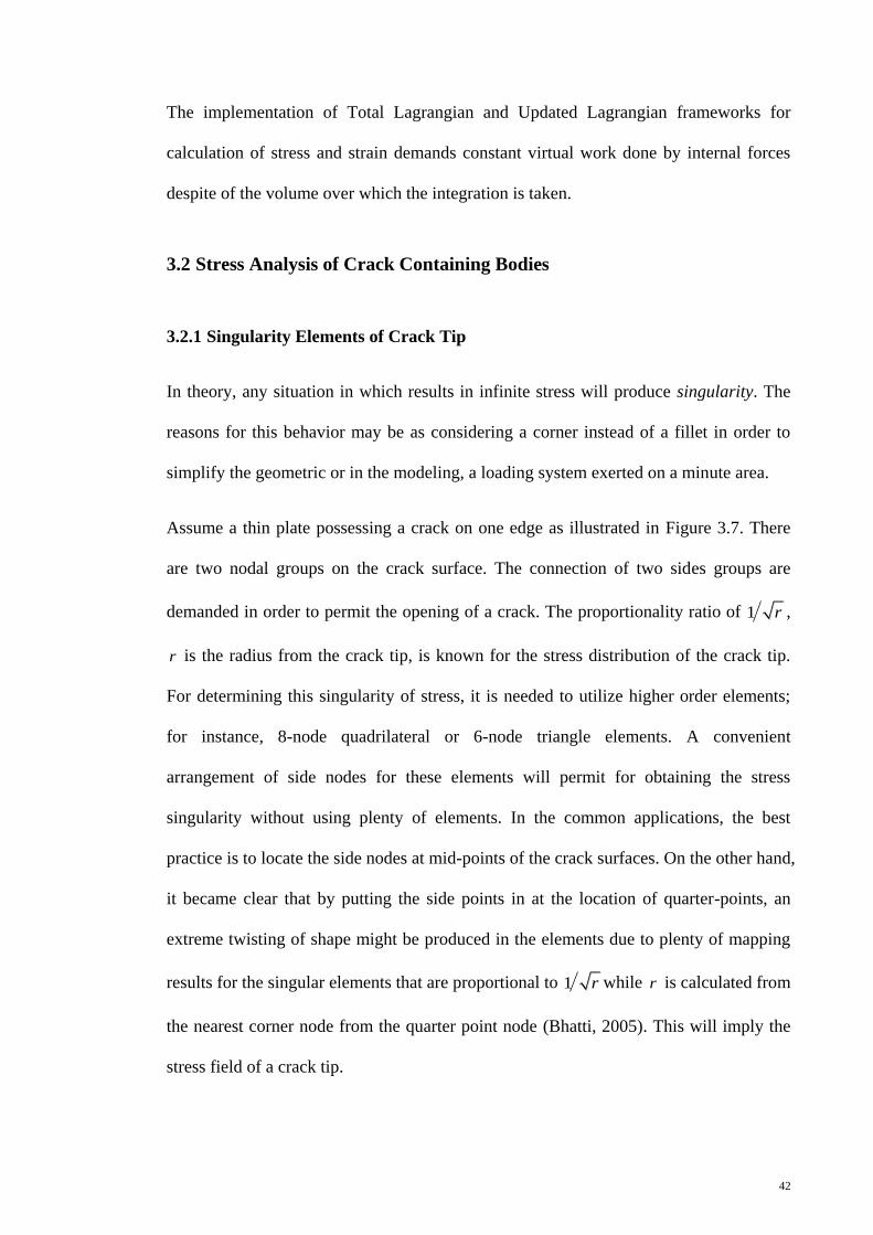
Assume a thin plate possessing a crack on one edge as illustrated in Figure 3.7. There
are two nodal groups on the crack surface. The connection of two sides groups are
demanded in order to permit the opening of a crack. The proportionality ratio of 1 r ,
r is the radius from the crack tip, is known for the stress distribution of the crack tip.
For determining this singularity of stress, it is needed to utilize higher order elements;
for instance, 8-node quadrilateral or 6-node triangle elements. A convenient
arrangement of side nodes for these elements will permit for obtaining the stress
singularity without using plenty of elements. In the common applications, the best
practice is to locate the side nodes at mid-points of the crack surfaces. On the other hand,
it became clear that by putting the side points in at the location of quarter-points, an
extreme twisting of shape might be produced in the elements due to plenty of mapping
results for the singular elements that are proportional to 1 r while r is calculated from
the nearest corner node from the quarter point node (Bhatti, 2005). This will imply the
stress field of a crack tip.

43
Figure 3.7 A meshed thin plate model containing edged-crack with quarter-point elements (Bhatti, 2005)
For comprehensive understanding, assume edge of 1-2-3 as displayed in Figure 3.7 with
the coordinate of 0, / 4a and a respectively from node 1. Their multiplication by
quadratic Lagrangian interpolation will result in the mapping of aforementioned edge as,
2
1 10 1 1 1 1
2 4 2
11
4
ar s s s s a s s
a s
(3.47)
The horizontal displacement of the same edge by applying similar interpolation function
is,
1 2 3
1 2 3
1 11 1 1 1
2 2
11 2 1 1 1
2
u u s s u s s u s s
s su s s u s s u
(3.48)
By deriving the u with respect to r , it results in axial strain. With the application of
chain rule accompanied with the inversion of the mapping, the derivative of u with
respect to r will be as,
1 2 12 1 4 2 1
1
du du dr du du ds
ds dr ds dr dr ds
s u su s u
a s
(3.49)
Where,
44
1 2 3
2
(4 3 ) 4( 2 ) ( 4 )
2
r as
a
r a u a r u a r udu
dr ra
(3.50)
The last equation implies the proportionality of strain with 1 r and as the stress is also
proportional to the strain, so same proportionality ratio is governs at the crack tip.
Therefore, by placing side nodes at the quarter-points produces demanded element
stress singularity. In practical fracture analysis, the same pattern as Figure 3.7 is
implemented without applying any specific element or refining process (Bhatti, 2005).
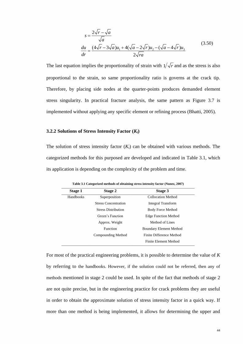
3.2.2 Solutions of Stress Intensity Factor (Ki)
The solution of stress intensity factor (Ki) can be obtained with various methods. The
categorized methods for this purposed are developed and indicated in Table 3.1, which
its application is depending on the complexity of the problem and time.
Table 3.1 Categorized methods of obtaining stress intensity factor (Nunez, 2007)
Stage 1 Stage 2 Stage 3
Handbooks Superposition
Stress Concentration
Stress Distribution
Green’s Function
Approx. Weight
Function
Compounding Method
Collocation Method
Integral Transform
Body Force Method
Edge Function Method
Method of Lines
Boundary Element Method
Finite Difference Method
Finite Element Method
For most of the practical engineering problems, it is possible to determine the value of K
by referring to the handbooks. However, if the solution could not be referred, then any of
methods mentioned in stage 2 could be used. In spite of the fact that methods of stage 2
are not quite precise, but in the engineering practice for crack problems they are useful
in order to obtain the approximate solution of stress intensity factor in a quick way. If
more than one method is being implemented, it allows for determining the upper and

45
lower limits of answer. For high precision repeating measurements of stress intensity
factor one of the numerical methods of stage 3 may be applied. The method selecting
will be affected by nature and complexity of the problem. Researchers and engineers in
the field of fracture mechanics are mostly applying the finite element method. The
determination of stress intensity factor can be implemented in two ways: (a) direct
approaches that define a direct correlation between stress intensity factor and finite
element results; (b) energy approaches that calculate the energy release rate in advance.
Practically, the energy approaches are more precise and reliable. Nevertheless, the direct
approaches can be useful for verifying the results of energy approaches. The main
approaches for stress intensity calculations might be named as displacement correlation,
which is a direct approach; strain energy release rate (G), which is an energy approach;
crack tip opening displacement (CTOD), which is a direct approach and J-integral based
on energy approach (Nunez, 2007).
3.2.2.1 Displacement Correlation Approach
With a crack tip as a singular point, the stress distribution is tedious to determine with
finite element methods even with the application of fine elements. However, by defining
very fine elements in LEFM of crack tips an approximate stress distribution for
determining the stress intensity factor is convenient. The evaluation of stress intensity
factors in various radiuses from the crack tip can be obtained by inserting displacements
in the corresponding analytical expressions of stress intensity factors (Mohammadi,
2008) for the plane stress as shown in.
2
2(1 )
b a
y y
I
u uK
r
(3.51)
2
2(1 )
b a
x xII
u uK
r
(3.52)

46
2
b b
III z zK u ur
(3.53)
For the plane strain problems, the substitution of * (1 ) is required.
Figure 3.8 Stress intensity factor extrapolation (Mohammadi, 2008)
An easy extrapolating process, as shown in Figure 3.8, might be implemented for
approximating the stress intensity factor of crack tip singularity.
3.2.2.2 Strain Energy Release Rate (G) Approach
The energy methods gives comprehensive understanding of fracture mechanism
accompanied with various analytical and numerical approaches in fracture mechanics.
The energy release rate for the crack tip obtains the rate change in potential energy of
the cracked member when the crack is growing. As a definition the strain energy release
rate is given by,
Ga
(3.54)
Where is the potential energy and in two-dimension a is the crack length. As it was
seen in the Equation (2.26) energy release rate is related to stress intensity factor as,
2
2 2
:Plane Stress
(1 ) :Plane Strain
i
i
K
EG
K v
E
(3.55)

47
3.2.2.3 Crack Tip Opening Displacement (CTOD) Approach
This approach mostly is being used in elastic-plastic fracture mechanics that fracture
happens while its corresponding value equal to the critical one.
Figure 3.9 Crack tip opening displacement
The mathematical definition of CTOD is as the distance when from the crack tip point
two 45 lines cross the crack’s surfaces as illustrated in Figure 3.9. From to the Irwin’s
results for Mode I fracture, the first-order solution of crack tip is,
1
22sin 1 2cos
2 2 2 2
Iy
K ru k
(3.56)
Where by replacing the value of crack tip opening at the radius of r will be
as (Mohammadi, 2008),
2
1
2
y
I
u
k rK
(3.57)
And in a similar way, the crack tip opening displacement for pr r , radius in the Irwin
plastic zone, will be obtained:
24 I
y
K
E
(3.58)

48
In the analysis of linear elastic fracture mechanics and also for brittle fracture such as
fracture in the glass, cracks are considered as sharp cracks and therefore the crack tip
opening displacement of will be zero. However, in the case of elastic-plastic fracture
and ductile fracture cannot be omitted which is due to large deformation of cracked
member (Mohammadi, 2008).
3.2.2.4 J-Integral Approach
By this concept introduced by (Rice, 1968), intending to define a path independent
integral around the singularity point of crack tip in order to measure the corresponding
stress-strain field as illustrated in Figure 3.10.
Figure 3.10 Arbitrary contour surrounding the singularity point of crack tip (Carlson, 1978).
The integration is performed to isotropic cracked bodies of linear or nonlinear elastic
materials with no body forces in two-dimension. Therefore, in order to define the field,
Rice (1968) proposed the J-Integral as,
ii
uJ wdy T ds
x
(3.59)
Where,
Arbitrary path around the crack tip
w Strain energy density and equal to 0
ij
ij ijd

49
iT Traction vector in the normal direction from and equal to ij jn
iu Displacement
s The length of arc along
On the other hand, Rice (1968) proposed an alternative definition for J-Integral with
respect to potential energy, as,
Ja
(3.60)
Which,
The potential energy per unit thickness
a The length of crack
By definition, in the case of LEFM the J-integral equals to strain energy release rate, G
(Carlson, 1978; Yoda, 1980). The relation of J-integral to stress intensity factor, K, is
through the energy release rate and for two situations of plane stress and plane strain is
as below,
2
2 2
:Plane Stress
(1 ) :Plane Strain
i
i
K
EJ G
K v
E
(3.61)

50
Chapter 4: Results and Discussions
Finite element methods based on the formulations of plates or shells are extensively
utilized by researchers and engineers to perform thin-wall analysis of various structures
such as aircrafts, ships or others. In order to have optimized design over these structures,
it is crucial to consider through thickness cracks as a majority causes of fractures. When
dealing with plates or shells the evaluation of Stress Intensity Factor can help for better
understanding of their behaviors in their case of being subjected to loading systems of
tensions, moments or shears. Crack tip analysis and the determination of bending stress
intensity factors and membrane stress intensity factors of plates subjected to transversal
loading has a great concern of researchers over decades. Although, many commercial
software for the simulation and analysis of plates under tension have been developed
and used by engineers, but the cracks analysis of plates under bending mostly has been
conducted by user’s subroutines and codes.
As illustrated in Figure 4.1, while a plate or shell has been subjected to a transversal
load, it is appeared that the crack has two more fracture modes in comparison to the
general fracture modes of Figure 2.8 which will account for out of plane bending or
torsional loadings. The parameters of stress resultant intensity factor (SRIF), 1K , 2K
and 3K are considered and implemented otherwise of using stress intensity factors (SIF)
of IK , IIK and IIIK (Dirgantara & Aliabadi, 2002) with having relationship as,
( ) 13
12I b b
zK K
h ( ) 23
12II b b
zK K
h
2
( ) 33
3 121
2III b b
zK K
h h
(4.1)

51
for bending loadings indexed with b,
( ) 13
1I m mK K
h
( ) 2
1II m mK K
h (4.2)
for membrane loadings indexed with m,
The evaluation of aforementioned relations can be implemented by variety of methods
such as energy, displacement extrapolation and the J-integral methods. In this study, the
determination of stress intensity factor throughout the stress resultant parameters has
conducted by using displacement extrapolation of the crack tip opening displacement.
Figure 4.1 Modes of fracture for a crack in plates: (a) and (b) membrane, (c) and (e) bending and torsion, (d) out of plane
shear (Palani, Iyer, & Dattaguru, 2006)
4.1 Displacement Extrapolation Technique
For modeling of a crack tip in LEFM problems various finite element methods based on
Reissner-Mindlin plate theories were presented which account for bending and shear

52
deformations. A crack tip can be modeled by using quadrilateral elements that normally
is deformed to the triangles, Figure 4.2.
Figure 4.2 Quadrilateral element into a triangle element transformation at the crack tip (Anderson, 2005)
For the analysis of elastic crack problems, the nodes that are located at the crack tip are
fixed and the mid points are transferred to the quarter points on the side. Consequently,
the singular element based on the 1/ r criterion is forming which results in
improvement in accuracy of the solution, Figure 4.3.
Figure 4.3 Formation of crack tip element with mid-points sliding to the quarter points (Anderson, 2005)
Generally, stress resultant intensity factor can be determined at any point of the crack
surface by using the equation in below (Purbolaksono et al., 2012).
1
,CK F w uL
(4.3)
which,

53
1 2 3 1 2b b b m mK K K K K K and 1 2 3 1 2,w u w w w u u
In above, iw and iu are the rotations and displacements of nodes with respect to the
coordinate system. As indicated in Figure 4.3, for points A-A´ and B-B´, initially
corresponding together, and from Equation (4.3) the related stress resultant intensity
factors for the two mentioned points are,
4, ,
AA A A
CK F w u w uL
(4.4)
4, ,
3
BB B B
CK F w u w uL
(4.5)
where
30 0 0 0
48 2
30 0 0 0
48 2
50 0 0 0
24(1 ) 2
0 0 0 2 08
0 0 0 0 28
Eh
Eh
EhC
Eh
Eh
F
(4.6)
Displacement extrapolation concept can be used to estimate the stress resultant intensity
factor of the crack tip (Dirgantara & Aliabadi, 2002; Purbolaksono et al., 2012).
tip BB AAAA
AA BB
rK K K
r r
(4.7)
In Equation (4.7) the AAr and BBr are implying the distance of their corresponding point
to the crack tip which are 1
4AAr L
and 3
4BBr L
.
4.2 Numerically Solved problems
There is various commercial CAE software such as ADINA, ANSYS®
, ALGOR,
ABAQUS and so on that can be used for finite element analysis simulations. ANSYS®
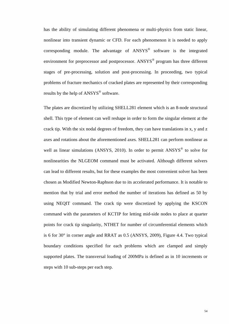
54
has the ability of simulating different phenomena or multi-physics from static linear,
nonlinear into transient dynamic or CFD. For each phenomenon it is needed to apply
corresponding module. The advantage of ANSYS®
software is the integrated
environment for preprocessor and postprocessor. ANSYS®
program has three different
stages of pre-processing, solution and post-processing. In proceeding, two typical
problems of fracture mechanics of cracked plates are represented by their corresponding
results by the help of ANSYS®
software.
The plates are discretized by utilizing SHELL281 element which is an 8-node structural
shell. This type of element can well reshape in order to form the singular element at the
crack tip. With the six nodal degrees of freedom, they can have translations in x, y and z
axes and rotations about the aforementioned axes. SHELL281 can perform nonlinear as
well as linear simulations (ANSYS, 2010). In order to permit ANSYS®
to solve for
nonlinearities the NLGEOM command must be activated. Although different solvers
can lead to different results, but for these examples the most convenient solver has been
chosen as Modified Newton-Raphson due to its accelerated performance. It is notable to
mention that by trial and error method the number of iterations has defined as 50 by
using NEQIT command. The crack tip were discretized by applying the KSCON
command with the parameters of KCTIP for letting mid-side nodes to place at quarter
points for crack tip singularity, NTHET for number of circumferential elements which
is 6 for 30° in corner angle and RRAT as 0.5 (ANSYS, 2009), Figure 4.4. Two typical
boundary conditions specified for each problems which are clamped and simply
supported plates. The transversal loading of 200MPa is defined as in 10 increments or
steps with 10 sub-steps per each step.

55
Figure 4.4 Singularity elements formation at the crack tip
Then, each increment was written into a separate load step file using LSWRITE
command. After reaching to the last increment transversal loading of 200MPa, the
LSSOLVE command implemented to solve the problem according to the load step files
from 1 to 10 which leads to their gradually results in the post-processing.
4.2.1 A Center Cracked Square Plate under Transversal Loading
A square plate with properties given in Table 4.1 Specifications of a square plate is
subjected to a transversal loading while the edges are fixed.
Table 4.1 Specifications of a square plate
Properties Symbol Quantity
Modulus of Elasticity E 210,000 MPa
Poisson’s ratio 0.3
Plate thickness h 0.5 mm
Plate width b 10 mm
Crack length a According to the diagrams
Loading increments 0q 0.2 MPa
Number of increments - 10
The magnitude of stress intensity factors for in-plane and out of plane shearing were
found to be insignificant in comparison to the in-plane opening stress intensity factor.
Therefore, the evaluations of IIK and IIIK were ignored. Bending stress intensity factor,
1bK , and membrane stress intensity factor, 1mK , were calculated by retrieving ANSYS®

56
results of nodal degree of freedoms for, respectively, about x-axis rotations and in x-axis
direction displacements of four carefully selected nodes in the neighborhood of crack tip
and on the crack surface accompanied with the displacement extrapolation method.
The calculated bending and membrane stress intensity factors from Equation (4.7) are
then being normalized by mean of (Purbolaksono et al., 2012),
1
1 4 2/
bbn
KK
Eh b a (4.8)
1
1 2 /
mmn
KK
Eh b a (4.9)
Figure 4.5 shows the considered geometry of the plate in both clamped and simply
supported boundary conditions. For generating the square plates it is requested to note
that b l . On the other hands, the value of l will vary for the rectangular plates.
a
b
l
(b)
a
b
l
(a)
Figure 4.5 Numerically solved problem as a plate with the clamped (a) and simply supported (b) boundary
conditions by finite element method

57
4.2.1.1 Clamped Square Plate
The corresponding results for bending stress intensity factor and membrane stress
intensity factor are depicted in Figure 4.6 and Figure 4.7, respectively.
From Figure 4.6, it is observed that the ranges of bending stress intensity factors are
much higher with respect to the membrane stress intensity factors. Hence, for the
membrane orientated applications, the effects of bending stresses must be accounted for
and dealt with precautions. Figure 4.6 shows that by increasing the transversal loading
the rate of changes in normalized bending stress intensity factor decreasing while the
normalized membrane stress intensity factor in Figure 4.7 shows vice versa. This is due
to this fact that by increasing the transversal loading the curvature of the plate is
increasing and therefore the extra loadings are transferred to the membrane stresses
rather than bending stresses. On the other hand, it is deducible that by increasing in the
crack lengths the bending of the plate is less responsible for the stresses.
Figure 4.6 Normalized bending stress intensity factor for a center-cracked square plate with clamped edges
0.00
0.10
0.20
0.30
0.40
0.50
0.60
0.70
0.80
0.90
0 20 40 60 80 100 120 140 160
K1
bn
qb4/Eh4
a/b=0.1
a/b=0.2
a/b=0.3
a/b=0.4
a

58
Figure 4.7 Normalized membrane stress intensity factor for a center-cracked square plate with clamped edges
4.2.1.2 Simply-Supported Square Plate
When a plate is restricted by simply supported boundary conditions, edges of the plate
can have rotations about the corresponding axes parallel to them with not letting for any
rotations around the other axes. In this way, the results of normalized bending stress
intensity factor and membrane stress intensity factor for mode I of fractures can be
depicted in Figure 4.8 and Figure 4.9.
The overall behaviors of the plate in two different boundary conditions of clamped and
simply supported edges are similar. By comparing Figure 4.6 and Figure 4.8, it is seen
that there is no considerable deviations in bending stress intensity factor. It implies that
for transversal loading of clamped and simply supported plates the bending stresses are
reasonably same as each other. In contrast, Figure 4.7 and Figure 4.9 show that by
replacing the clamped edges boundary condition into the simply supported ones the
amount of membrane stresses increasing significantly.
0.0000
0.0005
0.0010
0.0015
0.0020
0.0025
0.0030
0 20 40 60 80 100 120 140 160
K1
mn
qb4/Eh4
a/b=0.1
a/b=0.2
a/b=0.3
a/b=0.4a

59
Figure 4.8 Normalized bending stress intensity factor for a center-cracked square plate with simply supported edges
Figure 4.9 Normalized membrane stress intensity factor for a center-cracked square plate with simply supported edges
4.2.2 A Center Cracked Rectangular Plate under Transversal Loading
It is of interest to perform stress intensity factor calculations of different geometries in
order to have a better knowledge of them. Therefore, to have a comparative study a
0.00
0.10
0.20
0.30
0.40
0.50
0.60
0.70
0.80
0 20 40 60 80 100 120 140 160
K1
bn
qb4/Eh4
a/b=0.1
a/b=0.2
a/b=0.3
a/b=0.4
a
0.0000
0.0010
0.0020
0.0030
0.0040
0.0050
0.0060
0.0070
0 20 40 60 80 100 120 140 160
K1
mn
qb4/Eh4
a/b=0.1
a/b=0.2
a/b=0.3
a/b=0.4a

60
plate with rectangular shape is considered as the geometry having fixed crack length of
2.0mm but various heights. The other specifications of the plate are same as previous.
4.2.2.1 Clamped Rectangular Plate
The results of bending stress intensity factors and membrane stress intensity factors of
different range of height of the plate are illustrated in Figure 4.10 and Figure 4.11,
respectively.
The ranges of bending and membrane stress intensity factors in the case of rectangular
plates are lower than the range of bending and membrane stress intensity factors for the
square plates in both boundary conditions of clamped and simply supported edges.
Figure 4.10 Normalized bending stress intensity factor for a center-cracked rectangular plate with clamped edges
0.00
0.05
0.10
0.15
0.20
0.25
0.30
0.35
0.40
0.45
0 20 40 60 80 100 120 140 160
K1
bn
qb4/Eh4
a/b=0.2, b/l=0.5
a/b=0.2, b/l=0.625
a/b=0.2, b/l=2

61
Figure 4.11 Normalized membrane stress intensity factor for a center-cracked rectangular plate with clamped edges
The comparison of Figure 4.10 and Figure 4.11 with corresponding conditions of square
plate in Figure 4.6 and Figure 4.7 are showing a significant change in their behavior
when applying variety of heights for the plates.
By considering a plate with the ratio of 2b l , which simply implies a shorter plate,
when has clamped edges the amount of bending stress intensity factor increasing by
raising the transversal loading which contradicting with the case of square plate. And
likewise, with higher transversal loading the membrane stress intensity factor does not
have any considerable changes which were highest in the square plate. Therefore, it can
be inferred that with increasing the ration of b l above unity the stresses are mostly
related to the bending rather than membrane stresses.
0.0000
0.0001
0.0001
0.0002
0.0002
0.0003
0.0003
0.0004
0.0004
0.0005
0.0005
0 20 40 60 80 100 120 140 160
K1
mn
qb4/Eh4
a/b=0.2, b/l=0.5
a/b=0.2, b/l=0.625
a/b=0.2, b/l=2

62
4.2.2.2 Simply-Supported Rectangular plate
With simply supported edges for a rectangular plate subjected to incrementally
increasing transversal loading, the results might be as displayed in Figure 4.12 and
Figure 4.13.
As it was seen in the square plate possessing simply supported edges, Figure 4.9, for the
case of rectangular plate it is evident that by immigrating from clamped edges into the
simply supported ones the membrane stress field is increasing. However, the amount of
stress intensity factor for the condition of 2b l is not insignificant anymore and
simply supported boundary condition cause in increase of membrane stresses. Moreover,
the same behavior of rapid increase in the bending stress intensity factor is observed in
here as well with amplified effect.
Figure 4.12 Normalized bending stress intensity factor for a center-cracked rectangular plate with simply supported
edges
0.00
0.10
0.20
0.30
0.40
0.50
0.60
0.70
0.80
0 20 40 60 80 100 120 140 160
K1
bn
qb4/Eh4
a/b=0.2, b/l=0.5
a/b=0.2, b/l=0.625
a/b=0.2, b/l=2

63
Figure 4.13 Normalized membrane stress intensity factor for a center-cracked rectangular plate with simply supported
edges
In overall, the bending stress factor of center cracked square plate having clamped edges
boundary condition had the highest amount among the other conditions.
0.0000
0.0001
0.0002
0.0003
0.0004
0.0005
0.0006
0.0007
0.0008
0.0009
0 20 40 60 80 100 120 140 160
K1
mn
qb4/Eh4
a/b=0.2, b/l=0.5
a/b=0.2, b/l=0.625
a/b=0.2, b/l=2

64
Chapter 5: Conclusion
In this study, general introduction and methodology of fracture mechanics analysis of
plate are developed. The geometrical nonlinearities are due to large deformation or
rotation. Two major theories in the analysis of plates consist of Kirchhoff and Reissner-
Mindlin plate theories which former is suited for thin plates and latter for thicker plates.
In order to perform geometrically nonlinear plate analysis, bending problems includes
the interaction of plate out of plane bending and membrane loadings.
The incremental iterative techniques were presented with indicating their characteristics
and stated that the choice of each technique is directly is affected by the nature of the
problem in hand and other parameters such as time, economically agreeability of them.
In the fracture analysis of cracked plates the definition of singularity point is crucial and
this must be noticed that stress fields are proportional to the distance from the crack tip
as the ratio of 1/ r . It was seen that in the bending of plates the amount of stress
intensity factor for mode I of fracture has significantly high and therefore more
interesting for engineers to be considered. Hence, the calculations of stress intensity
factor for other modes were ignored. Different methods for the crack tip calculations of
stress intensity factor were proposed which among them crack tip displacement method
were found to be more convenient and straight forward for implementation based on
specifically formed elements at the crack tip. 8-node quadrilateral elements were well
suited to form in the crack tip with the mid-side nodes sliding to the quarter points
relative to the crack tip. These elements were defined based on the Mindlin plate theory

65
and therefore has the tolerance of being used for shear deformations. The commercial
finite element method code of ANSYS®
software was utilized throughout the
computations and relative nodal degree of freedom results for nodes in the
neighborhood of crack tip were retrieved by ANSYS®
. During the implementation of
ANSYS®
codes, it was noticed that by applying modified Newton-Raphson method with
carefully selected numbers of iterations and sub-steps both accuracy and time are
reserved. From the retrieved nodal data, it was a best practice to apply displacement
extrapolation method to predict the stress intensity factor at the crack tip by the help of
selected nodes on the crack edge in the vicinity of crack tip. Two different finite
element method simulations of geometrically nonlinear plate structures were developed.
A square and a rectangular plate possessing a center crack were subjected to different
boundary conditions of clamped and simply supported edges separately. In both
examples, the range of bending stress intensity factors was higher than the membrane
stress intensity factor. Bending stress intensity factor and membrane stress intensity
factor had two different behaviors which former had negative rate of changes and latter
had positive rate of changes. The reason for that was related to increasing in the
curvature of the plate while exerting more transversal loading which results in stress
transferring from bending situation to the membrane. Moreover, increasing the length of
cracks will decrease the bending stress intensity factor. From a simply supported square
plate it was inferred that membrane stress intensity factor is increasing in comparison to
a clamped square plate. The interesting change in behavior was observed for a
rectangular plate with longer edge in the direction of crack. By having aspect ratios of
upper than 1 with b l the bending stress intensity factor after a certain number of load
increments is increasing significantly while the membrane stress intensity factor is not

66
having any considerable changes for the clamped edges condition but has comparable
amount for the simply supported edges.
In the Linear Elastic Fracture Mechanics (LEFM) of plates, the equality in energy
release rate and the J-integral calculations makes the possibility of aforementioned
methods in defining stress intensity factor of the plate at the crack tip.

67
References
Anderson, T. L. (2005). Fracture Mechanics: Fundamentals and Applications: Taylor
& Francis.
ANSYS. (2009). ANSYS® Commands Reference Release 12.1: ANSYS, Inc.
ANSYS. (2010). ANSYS® Element Reference Release 12.1: ANSYS, Inc.
Barut, A., Madenci, E., Britt, V. O., & Starnes, J. H. (1997). Buckling of a thin, tension-
loaded, composite plate with an inclined crack. [doi: 10.1016/S0013-
7944(97)00064-7]. Engineering Fracture Mechanics, 58(3), 233-248.
Bhatti, A. (2005). Fundamental Finite Element Analysis and Applications: With
Mathematica and Matlab Computations: John Wiley & Sons.
Bower, A. F. (2009). Applied mechanics of solids: Taylor & Francis.
Broberg, K. B. (1999). Cracks and Fracture: Elsevier Science.
Carlson, K. W. (1978). A study of the experimental implementation and the resulting
characteristic behavior of the j-integral fracture toughness parameter applied to
two controlled-rolled steels. Ph.D. 7913403, University of Illinois at Urbana-
Champaign, United States -- Illinois. Retrieved from
http://search.proquest.com/docview/302880466?accountid=28930 ProQuest
Dissertations & Theses (PQDT) database.
Cook, R. D. (2001). Concepts and Applications of Finite Element Analysis: Wiley.
Datchanamourty, B. (2008). Nonlinear static, buckling and dynamic analysis of
piezothermoelastic composite plates using Reissner-Mindlin theory based on a
mixed hierarchic finite element formulation. Ph.D. 3301319, University of
Kentucky, United States -- Kentucky. Retrieved from
http://search.proquest.com/docview/304551797?accountid=28930 ProQuest
Dissertations & Theses (PQDT) database.
Desai, Y. M. (2011). Finite Element Method with Applications in Engineering: Pearson
Education India.
Dirgantara, T., & Aliabadi, M. H. (2002). Stress intensity factors for cracks in thin
plates. Engineering Fracture Mechanics, 69(13), 1465-1486. doi:
http://dx.doi.org/10.1016/S0013-7944(01)00136-9
Duarte Filho, L. A., & Awruch, A. M. (2004). Geometrically nonlinear static and
dynamic analysis of shells and plates using the eight-node hexahedral element

68
with one-point quadrature. Finite Elements in Analysis and Design, 40(11),
1297-1315. doi: 10.1016/j.finel.2003.08.012
Elices, M., Guinea, G. V., Gómez, J., & Planas, J. (2002). The cohesive zone model:
advantages, limitations and challenges. [doi: 10.1016/S0013-7944(01)00083-2].
Engineering Fracture Mechanics, 69(2), 137-163.
Liu, Y. J., & Riggs, H. R. (2002). Development of the MIN-N Family of Triangular
Anisoparametric Mindlin Plate Elements: University of Hawaii at Manoa.
Logan, D. L. (2011). A First Course in the Finite Element Method: Cengage Learning.
Madenci, E., & Guven, I. (2006). The Finite Element Method and Applications in
Engineering Using Ansys: Springer.
Mohammadi, S. (2008). Extended Finite Element Method: For Fracture Analysis of
Structures: John Wiley & Sons.
Nunez, D. (2007). J-integral computations for linear elastic fracture mechanics in h,p,k
mathematical and computational framework. M.S. 1450783, University of
Kansas, United States -- Kansas. Retrieved from
http://search.proquest.com/docview/304834836?accountid=28930 ProQuest
Dissertations & Theses (PQDT) database.
Palani, G. S., Iyer, N. R., & Dattaguru, B. (2006). A generalised technique for fracture
analysis of cracked plates under combined tensile, bending and shear loads.
Computers & Structures, 84(29–30), 2050-2064. doi:
10.1016/j.compstruc.2006.08.012
Perez, N. (2004). Fracture Mechanics: Springer.
Prathap, G. (1985). A simple plate/shell triangle. International Journal for Numerical
Methods in Engineering, 21(6), 1149-1156. doi: 10.1002/nme.1620210613
Purbolaksono, J., & Aliabadi, M. H. (2005). Large deformation of shear-deformable
plates by the boundary-element method. Journal of Engineering Mathematics,
51(3), 211-230. doi: 10.1007/s10665-004-6091-5
Purbolaksono, J., Dirgantara, T., & Aliabadi, M. H. (2012). Fracture mechanics analysis
of geometrically nonlinear shear deformable plates. Engineering Analysis with
Boundary Elements, 36(2), 87-92. doi: 10.1016/j.enganabound.2011.07.003
Reuter, W. G., Underwood, J. H., & Newman, J. C. (1995). Fracture Mechanics:
ASTM.
Rice, J. R. (1968). A Path Independent Integral and the Approximate Analysis of Strain
Concentration by Notches and Cracks. Journal of Applied Mechanics, 35(2),
379-386.
Sathyamoorthy, M. (1997). Nonlinear Analysis of Structures: Taylor & Francis.

69
Sosa, H. A., & Eischen, J. W. (1986). Computation of stress intensity factors for plate
bending via a path-independent integral. [Article]. Engineering Fracture
Mechanics, 25(4), 451-462. doi: 10.1016/0013-7944(86)90259-6
Szilard, R. (2004). Theories and Applications of Plate Analysis: Classical, Numerical,
and Engineering Methods: John Wiley.
Timoshenko, S., & Goodier, J. N. (1969). Theory of elasticity: McGraw-Hill.
Timoshenko, S., & Woinowsky-Krieger, S. (1959). Theory of plates and shells:
McGraw-Hill.
Ugural, A. C., & Fenster, S. K. (2003). Advanced strength and applied elasticity:
Prentice Hall PTR.
Ventsel, E., & Krauthammer, T. (2001). Thin Plates and Shells: Theory, Analysis, and
Applications: Marcel Dekker.
Wang, C. M., Reddy, J. N., & Lee, K. H. (2000). Shear Deformable Beams and Plates:
Relationships With Classical Solutions: Elsevier.
Yoda, M. (1980). The J-integral fracture toughness for Mode II. International Journal
of Fracture, 16(4), R175-R178. doi: 10.1007/bf00018247
Zienkiewicz, O. C. (1971). The finite element method in engineering science: McGraw-
Hill.
Zienkiewicz, O. C., & Taylor, O. C. Z. R. L. (2000). The Finite Element Method: Solid
Mechanics: Elsevier Science & Tech.