Copyright 2004 Society of Photo-Optical Instrumentation Engineers. This paper will be published in Proc. SPIE, Vol. 5165, and is made available as an electronic preprint with permission of SPIE. One print or electronic copy may be made for personal use only. Systematic or multiple reproduction, distribution to multiple locations via electronic or other means, duplication of any material in this paper for a fee or for commercial purposes, or modification of the content of the paper are prohibited.

Readout Modes and Automated Operation of the Swift X-Ray Telescope

J.E. Hill*a, D.N. Burrowsa, J.A. Nouseka, A.F. Abbeyc, R.M. Ambrosic, H. Bräuningere, W. Burkerte, S. Campanad, C. Cheruvua, G. Cusumanof, M.J. Freyberge, G.D. Hartnere, R. Klarb, C. Mangelsb, A. Morettid, K. Moria, D.C. Morrisa, A.D.T. Shortc, G. Tagliaferrid, D.J. Watsonc,

P. Woodb, A. Wellsc aDepartment of Astronomy & Astrophysics, Penn State University, USA,

bSouthwest Research Institute, USA, cPhysics & Astronomy Department, University of Leicester, UK, dINAF Osservatorio Astronomico di Brera, Milano, Italy,

eMax-Planck-Institut für extraterrestrische Physik, Garching bei München, Germany, fCNR Istituto di Fisica Cosmica ed Applicazioni dell Informatica, Italy

ABSTRACT The Swift X-ray Telescope (XRT) is designed to make astrometric, spectroscopic, and photometric observations of X-ray emission from Gamma-ray Bursts and their afterglows in the energy band 0.2-10 keV. In order to provide rapid-response, automated observations of these randomly occurring objects without ground intervention, the XRT must be able to observe objects covering some seven orders of magnitude in flux, extracting the maximum possible science from each one. This requires a variety of readout modes designed to optimise the information collected in response to shifting scientific priorities as the flux from the burst diminishes. The XRT will support four major readout modes: imaging, two timing modes and photon-counting, with several sub-modes. We describe in detail the readout modes of the XRT. We describe the flux ranges over which each mode will operate, the automated mode switching that will occur and the methods used for collection of bias information for this instrument. We also discuss the data products produced from each mode. Keywords: CCDs, Gamma-Ray Bursts, X-rays, Swift, X-Ray Telescope, Centroiding, Readout Modes

1. INTRODUCTION The Swift satellite1 consists of three instruments. A wide field of view Gamma-ray telescope, the Burst Alert Telescope (BAT)2, which is triggered by the Gamma-ray Burst (GRB) and two narrow field of view instruments; an X-ray Telescope and an Ultra-Violet/Optical Telescope (UVOT)3. Immediately after the GRB is detected and located by the BAT, the spacecraft will slew to point both the narrow field instruments to the target GRB location. The 20-70 second time-to-target means that about 30 GRBs per year (about 1/3 of the total) will be observed by the narrow field instruments during the Gamma-ray Burst. It is expected that most GRBs detectable by the BAT will be bright enough in X-rays at the time pointing is acquired to produce high-quality position, spectral and timing measurements with the XRT. The XRT4,5 is a sensitive, autonomous X-ray imaging spectrometer designed to measure the flux, spectrum, and light curve of GRBs and afterglow over a wide dynamic range covering more than seven orders of magnitude in flux. XRT utilizes the flight spare FM3 mirror set from the JET-X program6: a grazing incidence Wölter 1 mirror set, with a focal length of 3.5 m and an effective area of 110 cm2 at 1.5 keV. The imaging array is a MAT-22 CCD7, consisting of 600 x 600 image pixels, each 40 µm x 40 µm with a plate scale of 2.36 arcsec. For a source flux of 1 mCrab, the instrument response is 0.7 counts/sec. The XRT operates in four main modes depending on the flux of the GRB. Immediately after the Spacecraft has slewed and settled on the target the XRT begins operation in Imaging mode from which the location of the GRB can be

* Correspondence: Email: jhill@astro.psu.edu: Phone: 1 814 865-7706; Fax: 1 814 865-9100; Penn State University, 2582 Gateway Drive, State College, PA 16801, USA

determined (when the flux is greater than 23 mCrab). In the other modes; which are Photodiode mode (flux between 62 Crab and 0.6 Crab), Windowed Timing mode (flux between 600 mCrab and 1 mCrab) and Photon-Counting mode (for fluxes below 1 mCrab) the XRT measures the light curve and the spectrum. For a newly detected GRB, the XRT will refine the BAT positions (~1-4' uncertainty) to better than 2.5 arcsec in XRT detector coordinates within 5 seconds of target acquisition for typical bursts, allowing ground-based optical telescopes to begin immediate spectroscopic observations of the afterglow. Because of the fast pointing and variable thermal environment of the satellite, to produce an accurate centroid of the GRB, it is necessary to monitor the alignment of the XRT with a Telescope Alignment Monitor (TAM). The TAM is used to measure the alignment offsets between the X-ray camera, mirrors and the spacecraft (S/C) star tracker mounted on the upper tube. The offsets from the TAM are used to calculate a position correction value, which in turn is used to determine an accurate centroid position of the GRB target in the field of view (FoV) of the X-ray Telescope to 5 arcsec in S/C coordinates. The brightest source in the XRT FoV during the initial observation will almost always be the GRB counterpart, thus the source position can be detected and sent to the ground-based observers for rapid follow-up. Once the source position is determined, the XRT will begin measuring its spectrum, for fluxes up to 1.5 Crab, and light curve (brightness variability), for fluxes up to 62 Crab, in Photodiode mode. In some cases, the XRT spectrum will measure the red shift of the GRB directly giving its distance.

2. INSTRUMENT MODES

2.1. Mode Sequence Table The Mode Sequence Table (MST) is the look-up table for all science modes of operation of the XRT, both in manual operation, used for engineering purposes, and in the automated state, the nominal operating state for XRT. The MST dictates which CCD waveform is used for each mode, at what count-rate the instrument should switch from one mode to another in auto state, and which mode it should switch to. It controls which mode of operation is applied; during slews, when the S/C is within 10 arcmin of the source and when the S/C settles on the target. It also controls what modes of operation are called according to whether the target is: a Pre-Planned Target (PPT; targets uploaded from the ground by mission planners as part of the observatory command load); Targets Of Opportunity (TOOs; targets found by other satellites and uploaded without re-planning the entire command load); or Automated Targets (AT; a GRB newly discovered by the BAT). The MST is stored in EEPROM memory and loaded into RAM memory on boot-up. Temporary changes to lines of the MST can be made by telecommand from the ground, for instance which CCD waveform is run by the sequencer in a particular mode and the mode count-rate switch points, allowing for system optimisations on orbit.

2.2. Image Mode; Centroiding Swift must transmit GRB positions to the ground within 100 seconds of the burst. The BAT position determination and the S/C slew-to-target can take up to 95 seconds, and so the XRT must determine the position of the GRB to an accuracy of better than 5 arcsec in less than 5 seconds. To acquire positions at the highest fluxes, the photons are allowed to pile-up (i.e. more than one X-ray per pixel) using a low gain imaging mode with one of two integration times. The CCD waveform integrates the first frame for 0.1 second and then, while clocking the data out at 6.6 µsec/pixel, a 2.5 second integration image is obtained. Initial processing occurs on the 0.1 second frame; if the software determines there are too few photons to calculate a centroid, the processing continues on the 2.5 second frame. If the software determines the image has a centroid sigma too large, or if the convergence term for two consecutive centroid calculations is not met, the software flushes the image and the store section and retakes an image. If an accurate centroid position is not calculated after 12 frames, the mode is aborted. Centroids are calculated for GRBs over a flux range from 23 mCrab in Long Image mode to 37 Crab in Short Image mode where, for fluxes greater than this, the amount of charge from the GRB in the centre of the point spread function (PSF) exceeds full well capacity of the CCD pixel.

2.2.1.

2.2.2.

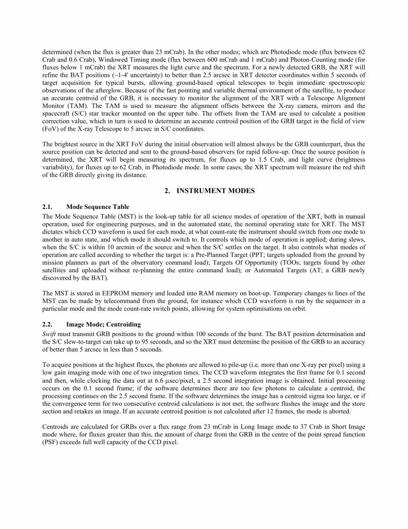
The Centroiding Algorithm In order to meet the timing and accuracy requirements a rapid and accurate centroiding algorithm is needed8,9. The algorithm must be robust in the presence of cosmic-ray events and detector defects. The algorithm for computing the centroid is divided into two phases, shown in Figure 1. Phase 1 - Phase 1 locates the wings of the GRB amidst the cosmic-rays and noise. This is done by locating the window with the maximum density of ‘isolated single pixel events’ or ISPEs. An ISPE is defined as an isolated pixel above the lower level discriminator (LLD) and below the upper level discriminator (ULD). From Figure 1 it can be seen that around the edge of the PSF there is a high density of isolated single pixel events in the image. Cosmic-rays almost always appear in the image as completely connected pixels without any ISPEs around them. Thus, Phase 1 effectively filters out cosmic rays while at the same time identifying the wings of the GRB. Phase 2 - The second phase starts by computing the centroid position using a ‘centre of gravity’ formula on the charge in the window derived from phase 1 positioned on the initial image. The window is then centred on this newly computed centroid and the centroid of this new window is again computed. This process of repositioning the window on the newly computed centroid is iterated until two successively computed centroid values coincide. The effect of Phase 2 is that a window is placed on the wings of the GRB sliding towards the centre until the centre of the window coincides with the actual centroid of the GRB due to the increasing density of X-rays from the edge towards the core.

PHASE 2

Phase 1 of the algorithm – Identification of the wings of the PSF.

Phase 2 – The iterative procedure moves the windowfrom the wings of the PSF to the centroid of the PointSource

Figure 1: XRT onboard computation of the GRB centroid

Centroiding Algorithm Parameters The algorithm requires five parameters;

1) The ‘Event Threshold’ - If a pixel contains an X-ray event its energy will fall between the lower level discriminator (LLD) and the upper level discriminator (ULD). The LLD is set to 140 dn which is 5 sigma above the noise floor.

2) The ‘Minimum number of events to centroid’ - if the total number of events is less than this parameter, the software processes the longer 2.5 sec integration frame. If this minimum is not met after processing 12 frames of data, an error type 1 is sent to the ground via the Tracking and Data Relay Satellite System (TDRSS). See section 3 for a discussion on the optimisation of this parameter.

3) The ‘Convergence parameter’ - this determines how close the successive values of the centroid should be before the algorithm stops iterating in phase 2. If after processing 12 frames this convergence parameter is not

met, the mode is aborted and an error type 2 is sent to the ground via TDRSS. The convergence parameter currently used in the centroiding algorithm is 0.0625 corresponding to 0.15 arcsec.

4) The ‘Window size’ - the size of the window used for locating the maximum ISPE density region in phase 1, and performing the iterative centroiding calculation in phase 2. A 50 x 50 window size has been determined to be optimum8.

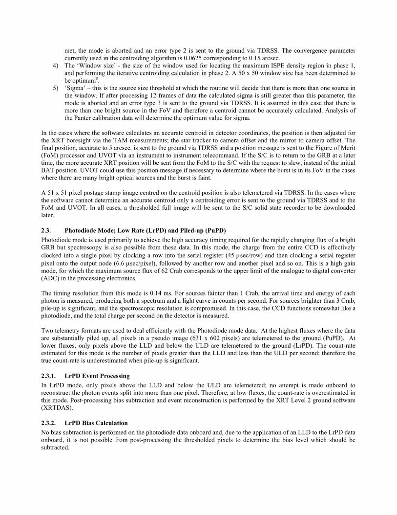
5) ‘Sigma’ – this is the source size threshold at which the routine will decide that there is more than one source in the window. If after processing 12 frames of data the calculated sigma is still greater than this parameter, the mode is aborted and an error type 3 is sent to the ground via TDRSS. It is assumed in this case that there is more than one bright source in the FoV and therefore a centroid cannot be accurately calculated. Analysis of the Panter calibration data will determine the optimum value for sigma.

In the cases where the software calculates an accurate centroid in detector coordinates, the position is then adjusted for the XRT boresight via the TAM measurements; the star tracker to camera offset and the mirror to camera offset. The final position, accurate to 5 arcsec, is sent to the ground via TDRSS and a position message is sent to the Figure of Merit (FoM) processor and UVOT via an instrument to instrument telecommand. If the S/C is to return to the GRB at a later time, the more accurate XRT position will be sent from the FoM to the S/C with the request to slew, instead of the initial BAT position. UVOT could use this position message if necessary to determine where the burst is in its FoV in the cases where there are many bright optical sources and the burst is faint. A 51 x 51 pixel postage stamp image centred on the centroid position is also telemetered via TDRSS. In the cases where the software cannot determine an accurate centroid only a centroiding error is sent to the ground via TDRSS and to the FoM and UVOT. In all cases, a thresholded full image will be sent to the S/C solid state recorder to be downloaded later.

2.3. Photodiode Mode; Low Rate (LrPD) and Piled-up (PuPD) Photodiode mode is used primarily to achieve the high accuracy timing required for the rapidly changing flux of a bright GRB but spectroscopy is also possible from these data. In this mode, the charge from the entire CCD is effectively clocked into a single pixel by clocking a row into the serial register (45 µsec/row) and then clocking a serial register pixel onto the output node (6.6 µsec/pixel), followed by another row and another pixel and so on. This is a high gain mode, for which the maximum source flux of 62 Crab corresponds to the upper limit of the analogue to digital converter (ADC) in the processing electronics. The timing resolution from this mode is 0.14 ms. For sources fainter than 1 Crab, the arrival time and energy of each photon is measured, producing both a spectrum and a light curve in counts per second. For sources brighter than 3 Crab, pile-up is significant, and the spectroscopic resolution is compromised. In this case, the CCD functions somewhat like a photodiode, and the total charge per second on the detector is measured. Two telemetry formats are used to deal efficiently with the Photodiode mode data. At the highest fluxes where the data are substantially piled up, all pixels in a pseudo image (631 x 602 pixels) are telemetered to the ground (PuPD). At lower fluxes, only pixels above the LLD and below the ULD are telemetered to the ground (LrPD). The count-rate estimated for this mode is the number of pixels greater than the LLD and less than the ULD per second; therefore the true count-rate is underestimated when pile-up is significant.

2.3.1.

2.3.2.

LrPD Event Processing In LrPD mode, only pixels above the LLD and below the ULD are telemetered; no attempt is made onboard to reconstruct the photon events split into more than one pixel. Therefore, at low fluxes, the count-rate is overestimated in this mode. Post-processing bias subtraction and event reconstruction is performed by the XRT Level 2 ground software (XRTDAS).

LrPD Bias Calculation No bias subtraction is performed on the photodiode data onboard and, due to the application of an LLD to the LrPD data onboard, it is not possible from post-processing the thresholded pixels to determine the bias level which should be subtracted.

The bias for photodiode mode data will be calculated on the ground from the following information telemetered by the flight software in the LrPD data header for each pseudo frame;

1) The sum and sum of squares of all pixels below the LLD. 2) The number of pixels below the LLD. 3) The last 20 pixels from each pseudo frame.

2.4. Windowed Timing Mode and Bias Row Windowed Timing (WT) mode is a high gain mode used to achieve high resolution timing (2.2 ms) with 1-D position information and spectroscopy for a flux less than 600 mCrab where, for higher fluxes, the data become piled-up. The CCD waveform bins ten rows into the readout register (45 µsec/row). The first 205 pixels in each row are dumped onto the output node with no conversion by the ADC, and the next 200 pixels are clocked and converted at the standard XRT rate of 6.6 µsecs/pixel. The next ten rows are then binned in the serial register, overlapping the remaining 205 dump pixels with the first 205 dump pixels from the next ten rows. The window size can be adjusted by changing the CCD waveform called for in this mode by an uploadable parameter to the Mode Sequence Table and by an uploadable command to the data processing software. This will be adjusted on orbit according to the accuracy of the BAT error circle and the S/C attitude control system (ACS).

2.4.1. Bias Row Calculation A bias row is calculated from one WT frame consisting of 600 rows taken during each slew or in Manual State. A ULD, set to 3σ above the noise peak, is applied to the data. For the first WT row, any pixel below the ULD is added into the bias row at the corresponding x-position. For pixel positions where the pixel value exceeded the ULD a zero is inserted at the corresponding x-position. The second WT row is then averaged into the current bias row with a running mean length (RML) applied unless a zero exists at that position in the current bias row where, in this case, the full pixel value from the second WT row is added in. This continues for all 600 rows. It is assumed that the X-ray flux is low enough during the slew that, for each x-position in at least one of the 600 rows, a pixel value is below the ULD. The calculation is shown below, where N is the RML (currently a value of 3 is used), and i is the number of pixels added in to the mean at position x;

(ix)ColN1(ix)MeanCol

N1N(ix)MeanCol ii1i ×

+×

−

=+ [1]

A completely new bias row is calculated every slew, however if the bias row is aborted due to the S/C pointing within 10 arcmin of the target, the last bias row is retained and used.

2.4.2.

2.4.3.

Windowed Timing Event Processing For every row of Windowed Timing data the bias row is subtracted. If the bias row value is greater than the pixel value, its value is set to zero. No event recognition is applied to the data; every pixel above the LLD and below the ULD is sent to the ground. Post-processing event reconstruction is performed by XRTDAS.

Bad Pixel Column In anticipation of CCD degradation on orbit due to radiation damage from the SAA, bad pixel positions can be uploaded to the flight software. In Windowed Timing mode a bad pixel will actually constitute a bad column. These can be pixels which are bright in every row of a pseudo frame, flickering pixels which are bright in many rows of a pseudo frame or a blocked column which will not transfer charge out of the array. To prevent the telemetry and the onboard processing being dominated by these events the bad column positions, uploadable by telecommand, are skipped over during the processing.

2.5. Photon Counting Mode and Bias Map Photon Counting (PC) mode is the more traditional frame transfer operation of an X-ray CCD camera. This mode is high gain, 2.5 second integration, yielding 2-D position, spectroscopy and limited timing information. The row transfer time in this mode is 45 µsec and each pixel is clocked onto the output node at 6.6 µsec/pixel. The instrument is operated in this mode at very low fluxes to prevent pile-up from the relatively long integration time.

2.5.1.

2.5.2.

2.5.3.

Bias Map Calculation The bias map calculation is similar to the bias row calculation shown in equation 1. The bias map is calculated from five PC frames taken during a slew or in Manual State. A ULD is applied to the data to eliminate X-ray events and cosmic-rays. Any pixel below the ULD is added into the initial map at that xy-position, a zero is inserted into the map for all pixels positions where the value is greater than the ULD. The second frame is then averaged into the map with a running mean length applied unless a zero exists at that position in the current bias map. In this case, the full value for that pixel position in the second Photon Counting frame is inserted into the map. This continues for all five frames. It is assumed that the X-ray flux is low enough that for each xy-position, in at least one of the five frames, a pixel value is below the ULD. An RML of six and a ULD of 3σ of the noise peak is currently used for the bias map calculation. In Auto State, the bias map can be operated in one of two ways selected by ground command; a completely new bias map can be computed during the slew or it can be added into an existing map that was previously processed. The nominal operation is a continual update to an already existing bias map in accordance with the running mean length uploadable parameter. To create a new bias map with each slew requires a change to the Mode Sequence Table by ground command.

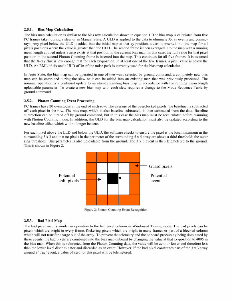
Photon Counting Event Processing PC frames have 20 overclocks at the end of each row. The average of the overclocked pixels, the baseline, is subtracted off each pixel in the row. The bias map, which is also baseline subtracted, is then subtracted from the data. Baseline subtraction can be turned off by ground command, but in this case the bias map must be recalculated before resuming with Photon Counting mode. In addition, the ULD for the bias map calculation must also be updated according to the new baseline offset which will no longer be zero. For each pixel above the LLD and below the ULD, the software checks to ensure the pixel is the local maximum in the surrounding 3 x 3 and that no pixels in the perimeter of the surrounding 5 x 5 array are above a third threshold; the outer ring threshold. This parameter is also uploadable from the ground. The 3 x 3 event is then telemetered to the ground. This is shown in Figure 2.

Potential split pixels

Guard pixels

Potential event

Figure 2: Photon Counting Event Recognition

Bad Pixel Map The bad pixel map is similar in operation to the bad pixel column in Windowed Timing mode. The bad pixels can be pixels which are bright in every frame, flickering pixels which are bright in many frames or part of a blocked column which will not transfer charge out of the array. To prevent the telemetry and the onboard processing being dominated by these events, the bad pixels are combined into the bias map onboard by changing the value at that xy-position to 4095 in the bias map. When this is subtracted from the Photon Counting data, the value will be zero or lower and therefore less than the lower level discriminator and discarded as an event. However, if the bad pixel constitutes part of the 3 x 3 array around a ‘true’ event, a value of zero for this pixel will be telemetered.

Due to the pixel values in Photon Counting mode having the possibility of being less than zero when baseline subtracted, an uploadable offset is added to every pixel to ensure every pixel is greater then zero. The only zero values telemetered to the ground are those bad pixels in the 3 x 3 surrounding area of a ‘true’ event.

2.6. Automated Mode Switching – Auto State XRT has two operating states; Auto and Manual. Auto State is the main operational state for the XRT; Manual State is only used for engineering and calibration purposes. Prior to going into Auto State the following conditions must be met;

1) The parameters for each operating mode configured 2) The TAM update rate set 3) A bias row and bias map calculated

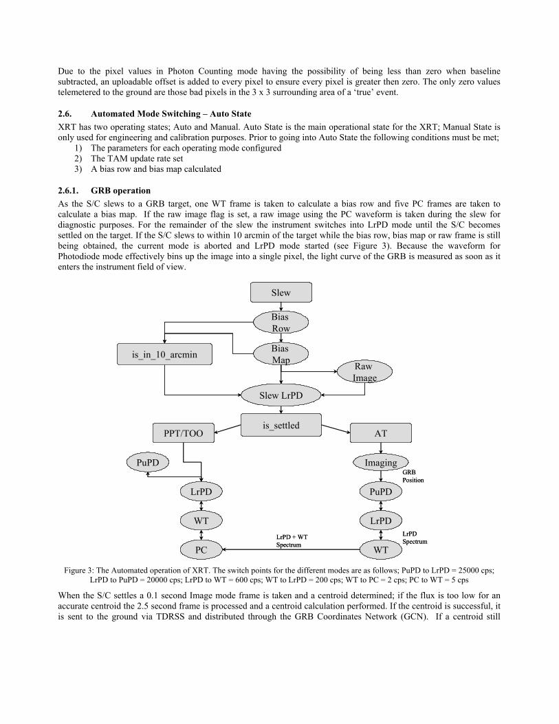
2.6.1. GRB operation As the S/C slews to a GRB target, one WT frame is taken to calculate a bias row and five PC frames are taken to calculate a bias map. If the raw image flag is set, a raw image using the PC waveform is taken during the slew for diagnostic purposes. For the remainder of the slew the instrument switches into LrPD mode until the S/C becomes settled on the target. If the S/C slews to within 10 arcmin of the target while the bias row, bias map or raw frame is still being obtained, the current mode is aborted and LrPD mode started (see Figure 3). Because the waveform for Photodiode mode effectively bins up the image into a single pixel, the light curve of the GRB is measured as soon as it enters the instrument field of view.

Slew

ATPPT/TOO

is_in_10_arcmin

PuPD

LrPD

WT

PC

PuPD

LrPD

WT

is_settled

Bias Row

Bias Map

Slew LrPD

Imaging

Raw Image

LrPDSpectrum

LrPD + WTSpectrum

GRB Position

Slew

ATPPT/TOO

is_in_10_arcmin

PuPD

LrPD

WT

PC

PuPD

LrPD

WT

is_settled

Bias Row

Bias Map

Slew LrPD

Imaging

Raw Image

LrPDSpectrum

LrPD + WTSpectrum

GRB Position

Figure 3: The Automated operation of XRT. The switch points for the different modes are as follows; PuPD to LrPD = 25000 cps;

LrPD to PuPD = 20000 cps; LrPD to WT = 600 cps; WT to LrPD = 200 cps; WT to PC = 2 cps; PC to WT = 5 cps

When the S/C settles a 0.1 second Image mode frame is taken and a centroid determined; if the flux is too low for an accurate centroid the 2.5 second frame is processed and a centroid calculation performed. If the centroid is successful, it is sent to the ground via TDRSS and distributed through the GRB Coordinates Network (GCN). If a centroid still

cannot be determined, short and long images continue to be taken for up to 12 frames. A centroid error message is telemetered through TDRSS if a centroid cannot be determined. After completing Imaging mode, the instrument then switches into the light curve mode of operation, where it switches between PuPD, LrPD, WT and PC modes depending on count-rate or flux, as shown in Figure 3. When the S/C is settled on the target and the GRB becomes faint enough that the instrument switches into LrPD mode, a raw spectrum is accumulated onboard from all the events above the LLD and below the ULD. When the instrument switches into Windowed Timing mode the spectrum is sent to the ground via TDRSS for ‘quick look’ purposes. The spectrum continues to be accumulated adding in the Windowed Timing mode data and, on switching to LrPD or PC mode, this spectrum is also telemetered through TDRSS. Due to the difference in gain between the two modes the first spectrum must be subtracted from the second spectrum on the ground by the Level 2 software. The mission level requirement imposed on XRT is to transmit the spectrum to the ground within 1200 seconds of the BAT trigger. Providing the GRB is not so bright that the instrument remains in PuPD or LrPD beyond this time, it has been shown through testing that XRT will meet this requirement. If the GRB should flare or become bright again XRT will switch up to a higher rate mode according to the count-rate. The ‘quick look’ spectra will only be sent out the first time the instrument switches from LrPD to WT and the first time it switches from WT to PC or back up into LrPD. The instrument will not return to imaging after switching into PuPD. This process is shown in Figure 3. To prevent the instrument from oscillating between two modes due to the Poisson variations in a constant source, the count-rates for switching down to a lower rate mode are higher than the count-rate for switching back up to the higher rate mode. The switch points for the different modes are as follows; PuPD to LrPD = 25000 cps; LrPD to PuPD = 20000 cps; LrPD to WT = 600 cps; WT to LrPD = 200 cps; WT to PC = 2 cps; PC to WT = 5 cps.

2.6.2.

2.6.3.

PPT and TOO Operation In order for Swift to be observing scientifically interesting objects around its orbit, the timeline between observable GRBs is filled in with Pre-Planned Targets (PPTs) and Targets of Opportunity (TOOs) by mission planners via observatory command load. Due to the low earth orbit, 600 km and 22°, a detected GRB will go out of view after approximately 20 minutes. Approximately 4 - 7 PPTs will be observed each orbit, these objects are not expected to be as bright as GRBs and therefore when the S/C settles on the target, XRT will go straight into LrPD and then continue in the light curve according to the count-rate measured onboard. If the target is extremely bright XRT will switch into PuPD, but it is unlikely that many of the PPTs will be bright enough for this mode. No Imaging mode data will be obtained, or quick-look spectra accumulated onboard, for PPTs and TOOs. This mode switching is outlined in Figure 3.

SAA Operation When the S/C enters the South Atlantic Anomaly (SAA) XRT switches into null mode to avoid flooding the telemetry stream with proton events. This is a non-data taking mode, but the CCD is constantly being clocked out to avoid the build up of charge. If the S/C should slew to a GRB while in the SAA, XRT will go into Imaging mode, attempt to calculate a position and take one PuPD mode frame before switching back into null mode. When exiting the SAA the XRT goes into the light curve part of the Mode Sequence Table switching into LrPD and, according to count-rate, into the appropriate mode. If the current target being observed is a GRB, a spectrum will be telemetered when switching from LrPD to WT and when it switches out of WT mode for the first time.

3. RESULTS

3.1. Imaging Mode Imaging mode was tested extensively at the MPE Panter Calibration Facility in Munich, Germany. This is the only time prior to launch that the capabilities of this mode can be fully tested, due the need for a focused image to optimise the centroiding algorithm parameters. The initial processing parameters were optimised prior to Panter using the flight algorithm written in “C” and processing data which had been obtained using the JET-X FM3 mirrors (XRT mirrors) and the XMM EPIC camera8,10,11. In order to finalise the parameters to meet the mission requirements with the onboard

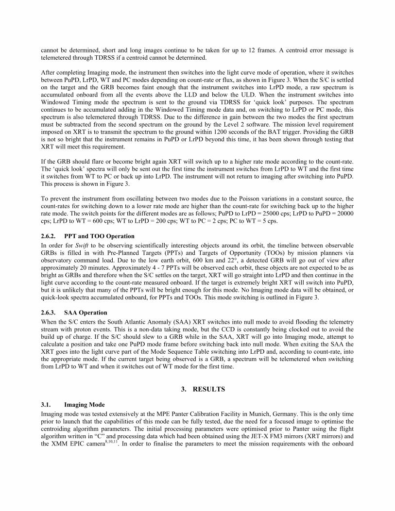
software, in terms of how quickly the centroid can be determined and to what accuracy, a wide range of fluxes and energies were tested with the integrated instrument. Figure 4 shows the Half Energy Width obtained using the Imaging mode waveform in raw data mode12. The focal length is slightly short, meaning a flatter PSF distribution across the FoV, which will benefit the centroiding algorithm. This means that for the GRBs which are positioned in the FoV according to the BAT position (accurate to 4 arcmin), and given the inaccuracy of the S/C ACS (up to 3 arcmin), that the PSF will not change significantly over the range of possible pointings.

Figure 4: Aluminium measurements using a Raw Data mode, showing the Half Energy Width is less than 20 arcsec across the field of

view at 1.5 keV12

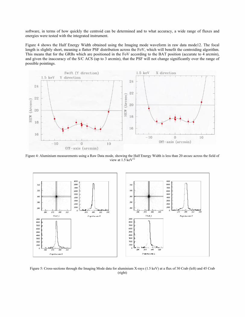
Figure 5: Cross-sections through the Imaging Mode data for aluminium X-rays (1.5 keV) at a flux of 30 Crab (left) and 45 Crab

(right)

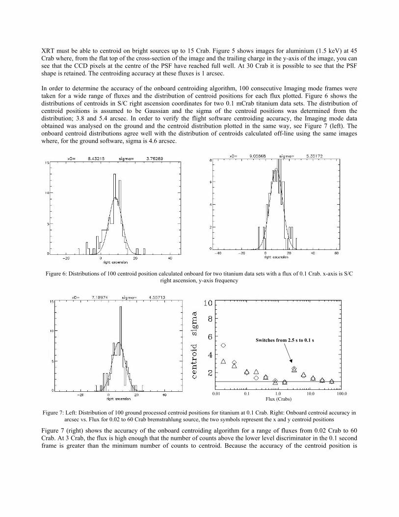
XRT must be able to centroid on bright sources up to 15 Crab. Figure 5 shows images for aluminium (1.5 keV) at 45 Crab where, from the flat top of the cross-section of the image and the trailing charge in the y-axis of the image, you can see that the CCD pixels at the centre of the PSF have reached full well. At 30 Crab it is possible to see that the PSF shape is retained. The centroiding accuracy at these fluxes is 1 arcsec. In order to determine the accuracy of the onboard centroiding algorithm, 100 consecutive Imaging mode frames were taken for a wide range of fluxes and the distribution of centroid positions for each flux plotted. Figure 6 shows the distributions of centroids in S/C right ascension coordinates for two 0.1 mCrab titanium data sets. The distribution of centroid positions is assumed to be Gaussian and the sigma of the centroid positions was determined from the distribution; 3.8 and 5.4 arcsec. In order to verify the flight software centroiding accuracy, the Imaging mode data obtained was analysed on the ground and the centroid distribution plotted in the same way, see Figure 7 (left). The onboard centroid distributions agree well with the distribution of centroids calculated off-line using the same images where, for the ground software, sigma is 4.6 arcsec.

Figure 6: Distributions of 100 centroid position calculated onboard for two titanium data sets with a flux of 0.1 Crab. x-axis is S/C

right ascension, y-axis frequency

1.0 10.0 100.00.10.01Flux (Crabs)

Switches from 2.5 s to 0.1 s

1.0 10.0 100.00.10.01Flux (Crabs)

Switches from 2.5 s to 0.1 s

Figure 7: Left: Distribution of 100 ground processed centroid positions for titanium at 0.1 Crab. Right: Onboard centroid accuracy in

arcsec vs. Flux for 0.02 to 60 Crab bremstrahlung source, the two symbols represent the x and y centroid positions

Figure 7 (right) shows the accuracy of the onboard centroiding algorithm for a range of fluxes from 0.02 Crab to 60 Crab. At 3 Crab, the flux is high enough that the number of counts above the lower level discriminator in the 0.1 second frame is greater than the minimum number of counts to centroid. Because the accuracy of the centroid position is

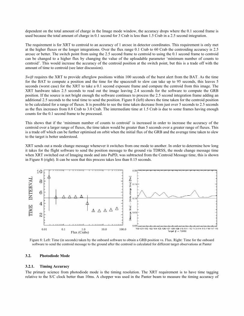
dependent on the total amount of charge in the Image mode window, the accuracy drops where the 0.1 second frame is used because the total amount of charge in 0.1 second for 3 Crab is less than 1.5 Crab in a 2.5 second integration. The requirement is for XRT to centroid to an accuracy of 1 arcsec in detector coordinates. This requirement is only met at the higher fluxes or the longer integrations. Over the flux range 0.1 Crab to 60 Crab the centroiding accuracy is 2.5 arcsec or better. The switch point from using the 2.5 second frame to centroid to using the 0.1 second frame to centroid can be changed to a higher flux by changing the value of the uploadable parameter ‘minimum number of counts to centroid’. This would increase the accuracy of the centroid position at the switch point, but this is a trade off with the amount of time to centroid (see later discussion). Swift requires the XRT to provide afterglow positions within 100 seconds of the burst alert from the BAT. As the time for the BAT to compute a position and the time for the spacecraft to slew can take up to 95 seconds, this leaves 5 seconds (worst case) for the XRT to take a 0.1 second exposure frame and compute the centroid from this image. The XRT hardware takes 2.5 seconds to read out the image leaving 2.4 seconds for the software to compute the GRB position. If the source is not bright enough the software continues to process the 2.5 second integration frame adding an additional 2.5 seconds to the total time to send the position. Figure 8 (left) shows the time taken for the centroid position to be calculated for a range of fluxes. It is possible to see the time taken decrease from just over 5 seconds to 2.5 seconds as the flux increases from 0.8 Crab to 3.0 Crab. The intermediate time at 1.5 Crab is due to some frames having enough counts for the 0.1 second frame to be processed. This shows that if the ‘minimum number of counts to centroid’ is increased in order to increase the accuracy of the centroid over a larger range of fluxes, the time taken would be greater than 5 seconds over a greater range of fluxes. This is a trade off which can be further optimised on orbit when the initial flux of the GRB and the average time taken to slew to the target is better understood. XRT sends out a mode change message whenever it switches from one mode to another. In order to determine how long it takes for the flight software to send the position message to the ground via TDRSS, the mode change message time when XRT switched out of Imaging mode and into PuPD, was subtracted from the Centroid Message time, this is shown in Figure 8 (right). It can be seen that this process takes less than 0.15 seconds.

1.0 10.0 100.00.10.01Flux (Crabs)

1.0 10.0 100.00.10.01 1.0 10.0 100.00.10.01Flux (Crabs)

Figure 8: Left: Time (in seconds) taken by the onboard software to obtain a GRB position vs. Flux. Right: Time for the onboard software to send the centroid message to the ground after the centroid is calculated for different target observations at Panter

3.2. Photodiode Mode

3.2.1. Timing Accuracy The primary science from photodiode mode is the timing resolution. The XRT requirement is to have time tagging relative to the S/C clock better than 10ms. A chopper was used in the Panter beam to measure the timing accuracy of

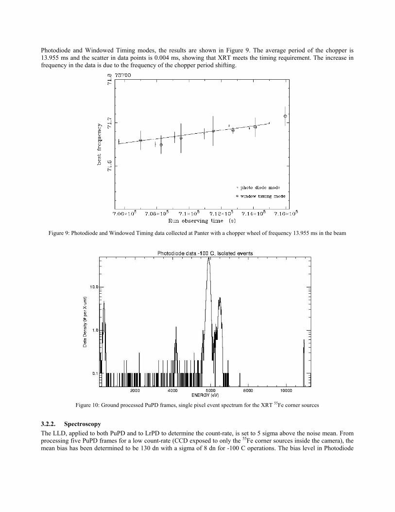
Photodiode and Windowed Timing modes, the results are shown in Figure 9. The average period of the chopper is 13.955 ms and the scatter in data points is 0.004 ms, showing that XRT meets the timing requirement. The increase in frequency in the data is due to the frequency of the chopper period shifting.

Figure 9: Photodiode and Windowed Timing data collected at Panter with a chopper wheel of frequency 13.955 ms in the beam

Figure 10: Ground processed PuPD frames, single pixel event spectrum for the XRT 55Fe corner sources

3.2.2. Spectroscopy The LLD, applied to both PuPD and to LrPD to determine the count-rate, is set to 5 sigma above the noise mean. From processing five PuPD frames for a low count-rate (CCD exposed to only the 55Fe corner sources inside the camera), the mean bias has been determined to be 130 dn with a sigma of 8 dn for -100 C operations. The bias level in Photodiode

mode may change around the orbit due to thermal variations and due to bright sources in the field. The LLD is fixed via telecommand prior to going into Auto State and so the calculated bias parameters are telemetered down for post-processing. Post-processing event recognition has been performed on the five PuPD frames and the results are shown in Figure 10. The full width half maximum (FWHM) of the event reconstructed PuPD and LrPD frames is 148 eV at 6keV, with a noise of 6.7 electrons. This spectroscopic resolution is retained for fluxes up to 1.5 Crab.

3.3. Windowed Timing Mode

3.3.1. Timing The timing resolution for windowed timing mode is shown in Figure 9 showing it meets the 10 ms time tagging requirement.

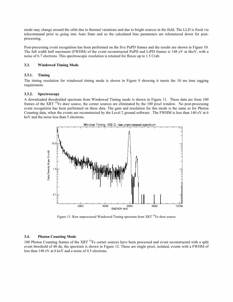
3.3.2. Spectroscopy A downloaded thresholded spectrum from Windowed Timing mode is shown in Figure 11. These data are from 100 frames of the XRT 55Fe door source, the corner sources are eliminated by the 100 pixel window. No post-processing event recognition has been performed on these data. The gain and resolution for this mode is the same as for Photon Counting data, when the events are reconstructed by the Level 2 ground software. The FWHM is less than 140 eV at 6 keV and the noise less than 5 electrons.

Figure 11: Raw unprocessed Windowed Timing spectrum from XRT 55Fe door source

3.4. Photon Counting Mode 100 Photon Counting frames of the XRT 55Fe corner sources have been processed and event reconstructed with a split event threshold of 40 dn, the spectrum is shown in Figure 12. These are single pixel, isolated, events with a FWHM of less than 140 eV at 6 keV and a noise of 4.5 electrons.

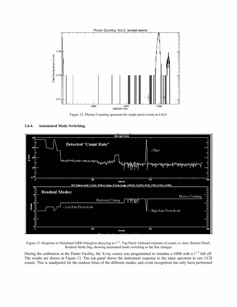
Figure 12: Photon Counting spectrum for single pixel events at 6 keV

2.6.4. Automated Mode Switching

Figure 13: Response to Simulated GRB/Afterglow decaying as t-1.3. Top Panel: Onboard estimate of counts vs. time. Bottom Panel: Readout Mode flag, showing automated mode switching as the flux changes

During the calibration at the Panter Facility, the X-ray source was programmed to simulate a GRB with a t-1.3 fall off. The results are shown in Figure 13. The top panel shows the instrument response to the input spectrum in raw CCD counts. This is unadjusted for the readout times of the different modes, and event recognition has only been performed

on the PC data. The bottom panel shows the modes corresponding to the change in flux, demonstrating the mode switching capability of the XRT.

4. CONCLUSIONS The XRT operating modes have been extensively tested at Panter, the requirement for the centroid position has been increased to 2.5 arcsec and the time to centroid waived for those fluxes where the time taken was slightly over 5 seconds. All other requirements are met. Various optimisations and improvements have been implemented in the flight software; some based on the Panter calibration findings and some on the testing performed at the S/C level, in particular from Day in the Life testing with the FoM, UVOT and the S/C which tested the full automated operation of the XRT. There is an on-orbit calibration plan, which will confirm the operating parameters in place. Furthermore, once on-orbit and GRBs are detected, additional optimisations of the flight software parameters are expected.

5. FURTHER WORK The implementation of the bias row and bias map is under consideration. Currently both the bias map and bias row are taken at the beginning of the slew to the next target. The bias map is added in to the stored bias map accumulated over previous slews and the bias row calculation creates a completely new bias row for each target. In the current mode of operation, if there are optically bright objects in the field of view when observing a GRB or pre-planned target, they will not be taken into account by the bias map and row. An alternative mode of operation, which will require an update to the onboard flight software and Mode Sequence Table, is to take a bias row before going into Windowed Timing for the first time and to take a bias map before going into Photon Counting for the first time.

ACKNOWLEDGEMENTS

This work was funded by NASA contract NAS5-00136

REFERENCES

1. J.A. Nousek et al., “Swift GRB Mission”, Proc. SPIE 5165, in press, 2004 2. S.D. Barthelmy et al., “Swift Burst Alert Telescope (BAT)”, Proc. SPIE 5165, in press, 2004 3. P.W.A. Roming et al., “Swift Ultra-Violet/Optical Telescope (UVOT)”, Proc. SPIE 5165, in press, 2004 4. D.N. Burrows et al., “Swift X-Ray Telescope (XRT)”, Proc. SPIE 5165, in press, 2004 5. D.N. Burrows, J.E. Hill, J.A. Nousek, A. Wells, A.D.T. Short, R.M. Ambrosi, G. Chincarini, O. Citterio, G.

Tagliaferri, “The Swift X-ray Telescope (XRT)”, Proc. SPIE 4851, p. 1320, 2002 6. O. Citterio, S Campana, P. Conconi, M. Ghigo, F. Mazzoleni, E. Poretti, G. Conti, G. Cusumano, B. Sacco, H.

Brauninger, W. Burkert, R. Eggert, C. Castelli and R. Willingale, “Characteristics of the flight model optics for the JET-X Telescope onboard the Spectrum-X-Γ satellite”, Proc. SPIE 2805, p. 56, 1996

7. A.D.T. Short, A. Keay, M.J.L. Turner, “Performance of the XMM EPIC MOS CCD Detectors”, Proc. SPIE 3445, p. 13, 1998

8. J.E. Hill, C. Cheruvu, A.F. Abbey, R.M. Ambrosi, D.N. Burrows, A.D.T. Short, A. Wells, J.A. Nousek , “An Algorithm for Locating PSF-Like Events and Computing the Centroid in X-ray Images”, Proc. SPIE 4851, p. 1347, 2001

9. R.M. Ambrosi, I.B. Hutchinson, , J.E. Hill, C. Cheruvu, A.F. Abbey A.D.T. Short, “The Impact of the In-orbit Background and the X-ray Source Intensity on the Centroiding Accuracy of the Swift X-ray Telescope”, NIM A: Vol. 493, 1-2, p. 67, 2002

10. R.M. Ambrosi, A.F. Abbey, I.B. Hutchinson, R. Willingale, S. Campana, G. Cusumano, W. Burkert, A. Wells, A.D.T. Short, O. Citterio, G. Tagliaferri, H. Brauninger, “Centroiding and Point Response Function Measurements of the Mirror/Detector Combination for the X-ray Telescope of the Swift Gamma Ray Burst Explorer”, Proc. SPIE 4497, p. 19, 2002

11. R. M. Ambrosi, A. F. Abbey, I. B. Hutchinson, R. Willingale, A. Wells, A.D.T. Short, S. Campana, O. Citterio, G. Tagliaferri, W. Burkert, H. Brauninger, “Point Spread Function and Centroiding Accuracy Measurements with the JET-X Mirror and MOS CCD Detector of the Swift Gamma Ray Burst Explorer's X-ray Telescope”, NIM A. Vol. 488, 3, p. 543, 2002

12. A. Moretti et al., “Swift XRT Point Spread Function Measured at the Panter End-to-End Tests”, Proc. SPIE 5165, 2004, in press