Embed Size (px)
Citation preview

1 / 166
Este documento incorpora firma electrónica, y es copia auténtica de un documento electrónico archivado por la ULL según la Ley 39/2015.Su autenticidad puede ser contrastada en la siguiente dirección https://sede.ull.es/validacion/
Identificador del documento: 960521Código de verificación: ThtRedGl
Firmado por: HARESH MANGHARAM CHULANI Fecha: 23/06/2017 18:03:30UNIVERSIDAD DE LA LAGUNA
JOSE MANUEL RODRIGUEZ RAMOS 23/06/2017 18:06:55UNIVERSIDAD DE LA LAGUNA
ERNESTO PEREDA DE PABLO 27/06/2017 14:59:25UNIVERSIDAD DE LA LAGUNA
Weighted Fourier Phase Slope as a Centroiding
Method in a Shack-Hartmann Wavefront Sensor for
Adaptive Optics in Astronomy
Haresh Mangharam Chulani
Submitted in partial fulfilment of the requirements
for the degree of Doctor of Philosophy in
Physics and Engineering
Thesis director: Dr. José Manuel Rodríguez Ramos
June, 2017

2 / 166
Este documento incorpora firma electrónica, y es copia auténtica de un documento electrónico archivado por la ULL según la Ley 39/2015.Su autenticidad puede ser contrastada en la siguiente dirección https://sede.ull.es/validacion/
Identificador del documento: 960521Código de verificación: ThtRedGl
Firmado por: HARESH MANGHARAM CHULANI Fecha: 23/06/2017 18:03:30UNIVERSIDAD DE LA LAGUNA
JOSE MANUEL RODRIGUEZ RAMOS 23/06/2017 18:06:55UNIVERSIDAD DE LA LAGUNA
ERNESTO PEREDA DE PABLO 27/06/2017 14:59:25UNIVERSIDAD DE LA LAGUNA

3 / 166
Este documento incorpora firma electrónica, y es copia auténtica de un documento electrónico archivado por la ULL según la Ley 39/2015.Su autenticidad puede ser contrastada en la siguiente dirección https://sede.ull.es/validacion/
Identificador del documento: 960521Código de verificación: ThtRedGl
Firmado por: HARESH MANGHARAM CHULANI Fecha: 23/06/2017 18:03:30UNIVERSIDAD DE LA LAGUNA
JOSE MANUEL RODRIGUEZ RAMOS 23/06/2017 18:06:55UNIVERSIDAD DE LA LAGUNA
ERNESTO PEREDA DE PABLO 27/06/2017 14:59:25UNIVERSIDAD DE LA LAGUNA
To my parents,

4 / 166
Este documento incorpora firma electrónica, y es copia auténtica de un documento electrónico archivado por la ULL según la Ley 39/2015.Su autenticidad puede ser contrastada en la siguiente dirección https://sede.ull.es/validacion/
Identificador del documento: 960521Código de verificación: ThtRedGl
Firmado por: HARESH MANGHARAM CHULANI Fecha: 23/06/2017 18:03:30UNIVERSIDAD DE LA LAGUNA
JOSE MANUEL RODRIGUEZ RAMOS 23/06/2017 18:06:55UNIVERSIDAD DE LA LAGUNA
ERNESTO PEREDA DE PABLO 27/06/2017 14:59:25UNIVERSIDAD DE LA LAGUNA

5 / 166
Este documento incorpora firma electrónica, y es copia auténtica de un documento electrónico archivado por la ULL según la Ley 39/2015.Su autenticidad puede ser contrastada en la siguiente dirección https://sede.ull.es/validacion/
Identificador del documento: 960521Código de verificación: ThtRedGl
Firmado por: HARESH MANGHARAM CHULANI Fecha: 23/06/2017 18:03:30UNIVERSIDAD DE LA LAGUNA
JOSE MANUEL RODRIGUEZ RAMOS 23/06/2017 18:06:55UNIVERSIDAD DE LA LAGUNA
ERNESTO PEREDA DE PABLO 27/06/2017 14:59:25UNIVERSIDAD DE LA LAGUNA
Acknowledgements
Very many people have, knowingly or unknowingly, contributed to the accomplishment of
the present work. Here is a list of just a few of them.
First of all, I would like to thank my thesis director, José Manuel Rodríguez Ramos, for his
guidance, advice, and always open, positive and optimistic attitude, from the commencement
till the completion of this work.
My special gratitude is for Ezequiel Ballesteros Ramírez, my colleague at the IAC (Instituto de
Astrofísica de Canarias), for transmitting me encouragement and motivation to perform a
research work like the present one, and for his thorough and disinterested revision of the full
text.
This work was executed in parallel with my participation in the EDiFiSE (Equalized and
Diffraction limited Field Spectrograph Experiment) project at the IAC, and received much
input from it. I would like to thank the former principal investigator of the project, Jesús
Jiménez Fuensalida, from whom I learnt about atmospheric turbulence characterization and
emulation, Luis Fernando Rodríguez Ramos for his ever readiness to discuss any (mainly
technical) topic, Ángel Alonso for the project management, Yolanda Martín for the FPGA and
user interface programming, Félix Gracia for his support in dealing with the optical system,
and Francesca Pinna and Enrique Joven for their help in the EMCCD (Electron Multiplying
Charge Coupled Device) camera characterization method validation.
I would also like to thank Jose Antonio Acosta Pulido, EDiFiSE’s present principal investigator,
and Luzma Montoya, also from the IAC, for providing me with uselful and relevant
bibliography.
Finally, I would like to express my gratitude to all my relatives and friends who have
understandingly allowed me the time and space and heartfeltly wished for the successful
completion of this work.

6 / 166
Este documento incorpora firma electrónica, y es copia auténtica de un documento electrónico archivado por la ULL según la Ley 39/2015.Su autenticidad puede ser contrastada en la siguiente dirección https://sede.ull.es/validacion/
Identificador del documento: 960521Código de verificación: ThtRedGl
Firmado por: HARESH MANGHARAM CHULANI Fecha: 23/06/2017 18:03:30UNIVERSIDAD DE LA LAGUNA
JOSE MANUEL RODRIGUEZ RAMOS 23/06/2017 18:06:55UNIVERSIDAD DE LA LAGUNA
ERNESTO PEREDA DE PABLO 27/06/2017 14:59:25UNIVERSIDAD DE LA LAGUNA

7 / 166
Este documento incorpora firma electrónica, y es copia auténtica de un documento electrónico archivado por la ULL según la Ley 39/2015.Su autenticidad puede ser contrastada en la siguiente dirección https://sede.ull.es/validacion/
Identificador del documento: 960521Código de verificación: ThtRedGl
Firmado por: HARESH MANGHARAM CHULANI Fecha: 23/06/2017 18:03:30UNIVERSIDAD DE LA LAGUNA
JOSE MANUEL RODRIGUEZ RAMOS 23/06/2017 18:06:55UNIVERSIDAD DE LA LAGUNA
ERNESTO PEREDA DE PABLO 27/06/2017 14:59:25UNIVERSIDAD DE LA LAGUNA
Sigh.- I caught this insight on the wing and quickly
took the nearest shoddy words to fasten it lest it
fly away from me. And now it has died of these
barren words and hangs and flaps in them – and I
hardly know any more, when I look at it, how I
could have felt so happy when I caught this bird.
(Friedrich Nietzsche: “The Gay Science”, book IV,
section 298)

8 / 166
Este documento incorpora firma electrónica, y es copia auténtica de un documento electrónico archivado por la ULL según la Ley 39/2015.Su autenticidad puede ser contrastada en la siguiente dirección https://sede.ull.es/validacion/
Identificador del documento: 960521Código de verificación: ThtRedGl
Firmado por: HARESH MANGHARAM CHULANI Fecha: 23/06/2017 18:03:30UNIVERSIDAD DE LA LAGUNA
JOSE MANUEL RODRIGUEZ RAMOS 23/06/2017 18:06:55UNIVERSIDAD DE LA LAGUNA
ERNESTO PEREDA DE PABLO 27/06/2017 14:59:25UNIVERSIDAD DE LA LAGUNA

9 / 166
Este documento incorpora firma electrónica, y es copia auténtica de un documento electrónico archivado por la ULL según la Ley 39/2015.Su autenticidad puede ser contrastada en la siguiente dirección https://sede.ull.es/validacion/
Identificador del documento: 960521Código de verificación: ThtRedGl
Firmado por: HARESH MANGHARAM CHULANI Fecha: 23/06/2017 18:03:30UNIVERSIDAD DE LA LAGUNA
JOSE MANUEL RODRIGUEZ RAMOS 23/06/2017 18:06:55UNIVERSIDAD DE LA LAGUNA
ERNESTO PEREDA DE PABLO 27/06/2017 14:59:25UNIVERSIDAD DE LA LAGUNA
Abstract
Among the latest developments in Adaptive Optics (AO) systems, Multi Object Adaptive
Optics (MOAO) systems span a large sensing field of view in the order of arcminutes, and
correct only the small portions of the sensed field of view where the scientific objects of
interest are situated, in the order of arcseconds each. Thus, they operate in open loop
correction mode, and their wavefront sensors need to deal with the large dynamic range of
the uncorrected atmospheric turbulence. This means that they need to be sensitive in low
light level scenarios as well as operate in larger fields of view as compared to the traditional
closed loop correction mode operation. Besides, Shack-Hartmann wavefront sensors (SHWFS)
continue to be the most widely employed and to have the most matured technology amongst
wavefront sensors to be found in astronomy applications.
The objective of the present work is to explore the performance of an innovative centroiding
algorithm at the subpupil image of a SHWFS, for point-like guiding sources. It has been named
Weighted Fourier Phase Slope, because it estimates the image’s displacement in the Fourier
domain by directly computing the phase slope at several spatial frequencies, without the
intermediate step of computing the phase; it then applies optimized weights to the phase
slopes at each spatial frequency obtained by a Bayesian estimation method. The idea has
been inspired by cepstrum deconvolution techniques, and this relationship is explained.
This algorithm’s tilt estimation performance is characterized and contrasted with other
known centroiding algorithms, such as Thresholded Centre of Gravity (TCoG) and Cross
Correlation (CC), through numerical simulations in Matlab™, first at a subpupil level. Figures
of merit such as computational cost, sensitivity in low light level conditions, linearity and
preferred field of view of operation, and robustness against atmospheric turbulence high
order aberrations of the spots, are all taken into account in open loop operation simulations.
Some effort has also been made to extend this comparison to a closed loop operation
situation. Results show a similar sensitivity to that of the CC algorithm, which is superior to
the one of the TCoG algorithm when big fields of view are necessary, i.e., in the open loop
correction case. On the other side, its advantage over the CC algorithm is an approximately
one order of magnitude lower computational cost. Also, as there is no threshold application
over the image, it is useful when the complete spot, including its low light level portion, is to
be considered for the centroid computation.
Numerical simulations are then extended to the complete sensor’s pupil with the aid of the
Object Oriented Matlab™ for Adaptive Optics (OOMAO) toolbox, thus including the sensor’s
fitting error in the simulations. Results are shown as Strehl Ratio (SR) or Encircled Energy (EE)
as a function of Natural Guide Star (NGS) magnitude, and are in good coincidence with the
subpupil level simulations.

10 / 166
Este documento incorpora firma electrónica, y es copia auténtica de un documento electrónico archivado por la ULL según la Ley 39/2015.Su autenticidad puede ser contrastada en la siguiente dirección https://sede.ull.es/validacion/
Identificador del documento: 960521Código de verificación: ThtRedGl
Firmado por: HARESH MANGHARAM CHULANI Fecha: 23/06/2017 18:03:30UNIVERSIDAD DE LA LAGUNA
JOSE MANUEL RODRIGUEZ RAMOS 23/06/2017 18:06:55UNIVERSIDAD DE LA LAGUNA
ERNESTO PEREDA DE PABLO 27/06/2017 14:59:25UNIVERSIDAD DE LA LAGUNA
10 Abstract
Finally, the laboratory optical setup of the EDiFiSE (Equalized and Diffraction limited Field
Spectrograph Experiment) project has been employed to corroborate the results obtained by
numerical simulations, and as a means to exemplify the algorithm’s tuning in a real case,
which is done by simulating the real system’s geometry. In this regard, the EDiFiSE’s EMCCD
(Electron Multiplying Charge Coupled Device) detector at the SHWFS has been characterized
and its gain and noise parameters have been measured and introduced in the simulated
model.
Pointing the way to the future, the necessary steps to test the algorithm at a telescope’s
adaptive optics system are devised. Also, the means to extend the applicability of the
algorithm to extended observed sources, such as with a Laser Guide Star (LGS) or in solar AO,
is proposed.

11 / 166
Este documento incorpora firma electrónica, y es copia auténtica de un documento electrónico archivado por la ULL según la Ley 39/2015.Su autenticidad puede ser contrastada en la siguiente dirección https://sede.ull.es/validacion/
Identificador del documento: 960521Código de verificación: ThtRedGl
Firmado por: HARESH MANGHARAM CHULANI Fecha: 23/06/2017 18:03:30UNIVERSIDAD DE LA LAGUNA
JOSE MANUEL RODRIGUEZ RAMOS 23/06/2017 18:06:55UNIVERSIDAD DE LA LAGUNA
ERNESTO PEREDA DE PABLO 27/06/2017 14:59:25UNIVERSIDAD DE LA LAGUNA
Table of contents
Abstract...................................................................................................................................... 9
Table of contents ..................................................................................................................... 11
List of figures ........................................................................................................................... 15
List of tables............................................................................................................................. 21
List of acronyms ....................................................................................................................... 23
Chapter 1. Atmospheric turbulence and adaptive optics ..................................................... 25
1.1. Imaging through turbulence............................................................................................. 25 1.1.1. The Kolmogorov turbulence model.................................................................................................... 25 1.1.2. The Fried Parameter r0 ....................................................................................................................... 27 1.1.3. Point Spread Function and Full Width Half Maximum ....................................................................... 29 1.1.4. Strehl Ratio and Encircled Energy....................................................................................................... 29
1.2. Adaptive Optics systems .................................................................................................. 30 1.2.1. Adaptive Optics compensation .......................................................................................................... 30 1.2.2. Sources of errors in adaptive optics system....................................................................................... 32
1.2.2.1. Anisoplanatism ........................................................................................................................... 32 1.2.2.2. Measurement error .................................................................................................................... 33 1.2.2.3. Deformable mirror fitting error .................................................................................................. 33 1.2.2.4. Temporal error............................................................................................................................ 34 1.2.2.5. Other sources of error ................................................................................................................ 34
1.2.3. Adaptive Optics system configurations .............................................................................................. 34 1.2.3.1. Single Conjugated Adaptive Optics (SCAO) systems .................................................................. 34 1.2.3.2. Ground Layer Adaptive Optics (GLAO) systems ......................................................................... 35 1.2.3.3. Multi-Conjugate Adaptive Optics (MCAO) systems.................................................................... 36 1.2.3.4. Multi-Object Adaptive Optics (MOAO) systems ......................................................................... 38
1.3. The Shack-Hartmann Wavefront Sensor (SHWFS) ............................................................. 39 1.3.1. Principles of operation ....................................................................................................................... 39 1.3.2. Image processing and phase recovery at the SHWFS ........................................................................ 41
1.3.2.1. Zonal methods for phase recovery ............................................................................................. 42 1.3.2.2. Modal methods for phase recovery. Zernike functions. ............................................................ 43
1.4. Centroiding methods in a SHWFS ..................................................................................... 45 1.4.1. Centre of Gravity (CoG) based methods ............................................................................................ 46
1.4.1.1. Thresholded centre of gravity (TCoG) ........................................................................................ 46 1.4.1.2. Weighted centre of gravity (WCoG) ........................................................................................... 46 1.4.1.3. Quad Cell (QC)............................................................................................................................. 47
1.4.2. Cross-Correlation (CC) method........................................................................................................... 47 1.4.3. Matched Filter (MF) method .............................................................................................................. 48
Chapter 2. Objective of the present work.............................................................................. 49
2.1. Motivation of the work.................................................................................................... 49
2.2. Objectives, methods and materials .................................................................................. 51

12 / 166
Este documento incorpora firma electrónica, y es copia auténtica de un documento electrónico archivado por la ULL según la Ley 39/2015.Su autenticidad puede ser contrastada en la siguiente dirección https://sede.ull.es/validacion/
Identificador del documento: 960521Código de verificación: ThtRedGl
Firmado por: HARESH MANGHARAM CHULANI Fecha: 23/06/2017 18:03:30UNIVERSIDAD DE LA LAGUNA
JOSE MANUEL RODRIGUEZ RAMOS 23/06/2017 18:06:55UNIVERSIDAD DE LA LAGUNA
ERNESTO PEREDA DE PABLO 27/06/2017 14:59:25UNIVERSIDAD DE LA LAGUNA
12 Table of contents
Chapter 3. The Weighted Fourier Phase Slope algorithm..................................................... 55
3.1. Fourier Phase Slope ......................................................................................................... 55 3.1.1. Further development of the Fourier phase slope formulation .......................................................... 58
3.2. Maximum-a-posteriori (MAP) weighting .......................................................................... 59
3.3. Comparison of computational cost of WFPS with other algorithms ................................... 61 3.3.1. Computational cost of the unidimensional and bi-dimensional FFT’s ............................................... 62
3.3.1.1. Computational cost of the unidimensional FFT.......................................................................... 62 3.3.1.2. Computational cost of the 2D-FFT .............................................................................................. 63
3.3.2. Computational cost of the WFPS algorithm ....................................................................................... 64 3.3.3. Computational cost of the TCoG and WCoG algorithms.................................................................... 66 3.3.4. Computational cost of the Cross Correlation algorithm .................................................................... 67 3.3.5. Comparison between algorithms through examples and conclusions .............................................. 68
Chapter 4. Numerical simulations at subpupil level ............................................................. 71
4.1. The simulation method.................................................................................................... 71 4.1.1. Simulation of Kolmogorov phase frames ........................................................................................... 71
4.1.1.1. Verification of the phase simulation method............................................................................. 74 4.1.2. Simulation of the pixelized images at the detector ........................................................................... 75 4.1.3. The Electron Multiplication CCD detector model .............................................................................. 77 4.1.4. Simulation workflow........................................................................................................................... 79
4.2. Linearity and dynamic range ............................................................................................ 81 4.2.1. Optimum field of view ........................................................................................................................ 84
4.3. MAP weights ................................................................................................................... 87
4.4. Sensitivity in the presence of detector noises and spot deformation ................................. 95
4.5. Effect of turbulence strength ........................................................................................... 99
4.6. Closed-loop operation simulation .................................................................................. 101
4.7. Square subaperture ....................................................................................................... 104
4.8. Conclusions of this chapter ............................................................................................ 108
Chapter 5. Numerical simulations at an entire pupil level ................................................. 111
5.1. The Object Oriented Matlab Adaptive Optics toolbox ..................................................... 111 5.1.1. Features added to the OOMAO in the context of the present work ............................................... 113 5.1.2. The simulation workflow .................................................................................................................. 115
5.2. Effect of estimating G-Tilt or Z-Tilt over the final PSF ...................................................... 118
5.3. Strehl Ratio as a function of NGS magnitude .................................................................. 122
5.4. Encircled Energy as a function of NGS magnitude ........................................................... 124
5.5. Conclusions of the present chapter ................................................................................ 125
Chapter 6. Laboratory tests ................................................................................................. 127
6.1. The EDiFiSE project ........................................................................................................ 127
6.2. The laboratory test ........................................................................................................ 128 6.2.1. The laboratory setup ........................................................................................................................ 128 6.2.2. Description of the test ...................................................................................................................... 129

13 / 166
Este documento incorpora firma electrónica, y es copia auténtica de un documento electrónico archivado por la ULL según la Ley 39/2015.Su autenticidad puede ser contrastada en la siguiente dirección https://sede.ull.es/validacion/
Identificador del documento: 960521Código de verificación: ThtRedGl
Firmado por: HARESH MANGHARAM CHULANI Fecha: 23/06/2017 18:03:30UNIVERSIDAD DE LA LAGUNA
JOSE MANUEL RODRIGUEZ RAMOS 23/06/2017 18:06:55UNIVERSIDAD DE LA LAGUNA
ERNESTO PEREDA DE PABLO 27/06/2017 14:59:25UNIVERSIDAD DE LA LAGUNA
Table of contents 13
6.2.3. Test results........................................................................................................................................ 131
6.3. Conclusions of this chapter ............................................................................................ 136
Chapter 7. General conclusions and future work ................................................................ 137
7.1. General conclusions....................................................................................................... 137
7.2. Future work .................................................................................................................. 138
Bibliography .......................................................................................................................... 141
Appendix A. Cepstrum analysis and homomorphic deconvolution .................................... 147
A.1. Definition of the complex cepstrum ............................................................................... 148
A.2. Homomorphic deconvolution ........................................................................................ 148
A.3. De-echoing a unidimensional signal ............................................................................... 151
A.4. De-echoing a bi-dimensional signal ................................................................................ 153
A.5. De-noising Shack-Hartmann subaperture images ........................................................... 154 A.5.1. High order aberrations in the spot................................................................................................... 155 A.5.2. Low light flux level ............................................................................................................................ 156 A.5.3. Limited field of view ......................................................................................................................... 157
Appendix B. Characterization of EDiFiSE’s EMCCD camera ................................................ 159

14 / 166
Este documento incorpora firma electrónica, y es copia auténtica de un documento electrónico archivado por la ULL según la Ley 39/2015.Su autenticidad puede ser contrastada en la siguiente dirección https://sede.ull.es/validacion/
Identificador del documento: 960521Código de verificación: ThtRedGl
Firmado por: HARESH MANGHARAM CHULANI Fecha: 23/06/2017 18:03:30UNIVERSIDAD DE LA LAGUNA
JOSE MANUEL RODRIGUEZ RAMOS 23/06/2017 18:06:55UNIVERSIDAD DE LA LAGUNA
ERNESTO PEREDA DE PABLO 27/06/2017 14:59:25UNIVERSIDAD DE LA LAGUNA

15 / 166
Este documento incorpora firma electrónica, y es copia auténtica de un documento electrónico archivado por la ULL según la Ley 39/2015.Su autenticidad puede ser contrastada en la siguiente dirección https://sede.ull.es/validacion/
Identificador del documento: 960521Código de verificación: ThtRedGl
Firmado por: HARESH MANGHARAM CHULANI Fecha: 23/06/2017 18:03:30UNIVERSIDAD DE LA LAGUNA
JOSE MANUEL RODRIGUEZ RAMOS 23/06/2017 18:06:55UNIVERSIDAD DE LA LAGUNA
ERNESTO PEREDA DE PABLO 27/06/2017 14:59:25UNIVERSIDAD DE LA LAGUNA
List of figures
Figure 1-1. Simplified schematic illustration of an adaptive optics system, by 2pem - Own work, CC
BY-SA 3.0, https://commons.wikimedia.org/w/index.php?curid=15279624 _____________ 30
Figure 1-2. Closed-loop vs Open-loop configurations of an AO system, from Marlon V., 2014. _____ 31
Figure 1-3. Angular anisoplanatism in AO systems, from Quiros F., 2007. _____________________ 32
Figure 1-4. SCAO system squematic diagram, from Quirós F. (2007) _________________________ 35
Figure 1-5. GLAO system squematic diagram, from Quirós F. (2007). _________________________ 36
Figure 1-6. MCAO system squematic diagrams, Star Oriented (left) and Layer Oriented (right), from
Quirós F. (2007). ____________________________________________________________ 37
Figure 1-7. Schematic comparison of MCAO (a) systems with MOAO (b) systems, from Gavel, 2006. 38
Figure 1-8. Schematic diagram of the Shack-Hartmann wavefront sensor operation, Rodríguez-
Ramos, 1998. ______________________________________________________________ 40
Figure 1-9. Fried geometry with corresponding ‘A’ matrices in a SHWFS as depicted in Herrmann,
1980. ____________________________________________________________________ 42
Figure 2-1. One dimensional representation of the relationship between image displacement and
linear phase slope shift in the Fourier domain, from Li, Huang and Gong, 2014. __________ 51
Figure 4-1. Comparison of theoretical Kolmogorov phase structure ([Eq. 4-1], solid line) with the
phase structure obtained from a series of 50000 simulated phase frames, with D/r0=1 and
32x32 pixels resolution per frame (diamond shapes). _______________________________ 74
Figure 4-2. Sketch of a high resolution image as is obtained with a 1024 x 1024 2D-FFT, and of the
final resolution image, obtained through decimation by block summation and selection of a
central FoV. _______________________________________________________________ 76
Figure 4-3. Schematic of the sources of noise in an Electron Multiplication Charge-Coupled Device._ 77
Figure 4-4. Core of the simulation workflow employed to compare the centroiding algorithms at a
subpupil level ______________________________________________________________ 79
Figure 4-5. (a) Estimated Z-Tilt as a function of applied Z-Tilt and FoV, for the WFPS algorithm with 4
x 4 spatial frequencies, circular subaperture with D/r0=2.5, Nyquist sampling, high light flux
level of 500000 photons, unity EMCCD gain, CIC=0.05 e-/pixel/frame, RON=50 e-r.m.s. (b)
Same for the TCoG algorithm. _________________________________________________ 82
Figure 4-6. (a) Estimated G-Tilt as a function of applied G-Tilt and FoV, for the WFPS algorithm with 4
x 4 spatial frequencies, circular subaperture with D/r0=2.5, Nyquist sampling, high light flux
level of 500000 photons, unity EMCCD gain, CIC=0.05 e -/pixel/frame, RON=50 e-r.m.s. (b)
Same for the TCoG algorithm. _________________________________________________ 83
Figure 4-7. (a) Estimated Z-Tilt as a function of applied Z-Tilt and centroiding algorithm, for a FoV of 8
x 8 pixels, circular subaperture with D/r0=2.5, Nyquist sampling, high light flux level of
500000 photons, unity EMCCD gain, CIC=0.05 e-/pixel/frame, RON=50 e-r.m.s. (b) Same for G-
Tilt estimation. _____________________________________________________________ 84

16 / 166
Este documento incorpora firma electrónica, y es copia auténtica de un documento electrónico archivado por la ULL según la Ley 39/2015.Su autenticidad puede ser contrastada en la siguiente dirección https://sede.ull.es/validacion/
Identificador del documento: 960521Código de verificación: ThtRedGl
Firmado por: HARESH MANGHARAM CHULANI Fecha: 23/06/2017 18:03:30UNIVERSIDAD DE LA LAGUNA
JOSE MANUEL RODRIGUEZ RAMOS 23/06/2017 18:06:55UNIVERSIDAD DE LA LAGUNA
ERNESTO PEREDA DE PABLO 27/06/2017 14:59:25UNIVERSIDAD DE LA LAGUNA
16 List of figures
Figure 4-8. Tilt estimation error in r.m.s. radians as a function of FoV and light flux level for the TCoG
algorithm (red), the CC algorithm (green) and the WFPS algorithm with 4 x 4 spatial
frequencies (blue), for Z-Tilt estimation (a) and G-Tilt estimation (b). D/r0 is 2.5. CIC is 0.05 e-
/pix/frame and RON is 50 e- rms. _______________________________________________ 85
Figure 4-9. Tilt estimation error in r.m.s. radians as a function of FoV and light flux level for the TCoG
algorithm (red), the CC algorithm (green) and the WFPS algorithm with at most 4 x 4 spatial
frequencies (blue), for Z-Tilt estimation (a) and G-Tilt estimation (b). D/r0 is 1. CIC is 0.05 e-
/pix/frame and RON is 50 e- rms. _______________________________________________ 86
Figure 4-10. Estimated tilt error in r.m.s. radians at the sensing wavelength as a function of incident
light level at the subaperture in photons and several schemes of spatial frequencies selection
for the WFPS algorithm (see text for further explanation). D/r0 is 2.5. Nyquist sampling. FoV is
14 by 14 pixels. EMCCD gain for each light level is high without saturating a 14 bits detector.
CIC is 0.05 e-/pixel/frame. RON is 50 e- rms. (a) is for Z-Tilt estimation and (b) for G-Tilt
estimation. ________________________________________________________________ 88
Figure 4-11. Estimated tilt error in r.m.s. radians at the sensing wavelength as a function of incident
light level at the subaperture in photons and several schemes of spatial frequencies selection
for the WFPS algorithm. D/r0 is 1. Nyquist sampling. FoV is 10 by 10 pixels. EMCCD gain for
each light level is high without saturating a 14 bits detector. CIC is 0.05 e -/pixel/frame. RON is
50 e- rms. (a) is for Z-Tilt and (b) for G-Tilt estimation. ______________________________ 92
Figure 4-12. Tilt estimation error in r.m.s. radians at the sensing wavelength as a function of incident
light level per subaperture in photons for the TCoG centroiding algorithm (red plots), CC
centroiding algorithm (green plots) and WFPS centroiding algorithm with 6 spatial
frequencies (blue plots). (a) is for Z-Tilt estimation with each subpanel for a different FoV:
10x10, 12x12, 14x14 and 16x16 pixels. (b) is for G-Tilt estimation, also with four subpanels
for the same values of FoV as for the Z-Tilt estimation case. For the 10x10 pixels FoV case, a
fourth algorithm corresponding to WFPS with 14X14 2D-FFT’s and 6 spatial frequencies has
been added, in cyan. D/r0 is 2.5. Nyquist sampling. EMCCD gain for each light level is high
without saturating a 14 bits detector. CIC is 0.05 e-/pixel/frame. RON is 50 e- rms. _______ 96
Figure 4-13. Tilt estimation error in r.m.s. radians at the sensing wavelength as a function of incident
light level per subaperture in photons for the TCoG centroiding algorithm (red plots), CC
centroiding algorithm (green plots) and WFPS centroiding algorithm with 6 spatial
frequencies (blue plots). (a) is for Z-Tilt estimation with each subpanel for a different FoV:
6x6, 8x8, 10x10 and 12x12 pixels. (b) is for G-Tilt estimation, also with four subpanels for the
same values of FoV as for the Z-Tilt estimation case. D/r0 is 1. Nyquist sampling. EMCCD gain
for each light level is high without saturating a 14 bits detector. CIC is 0.05 e -/pixel/frame.
RON is 50 e- rms. ___________________________________________________________ 98
Figure 4-14. Tilt estimation error in r.m.s. radians as a function of subpupil diameter to Fried
parameter ratio (D/r0) for incident light levels of 30, 50, 100, 200, 300 and 10000 photons
and two centroiding algorithms: TCoG and WFPS with 6 spatial frequencies selected. FoV
values are as per Table 4-8. (a) is for Z-Tilt estimation. (b) is for G-Tilt estimation. Nyquist
sampling. QE is 97%. EMCCD gain for each light level is high without saturating a 14 bits
detector. CIC is 0.05 e-/pixel/frame. RON is 50 e- rms. _____________________________ 100
Figure 4-15. Simulation of tilt estimation in a circular subaperture for closed loop operation and
D/r0=2.5. Estimation error in rms radians as a function of incident photons for Z-Tilt
estimation and a 10x10 pixels FoV (a), Z-Tilt estimation and a 12x12 pixels FoV (b), G-Tilt

17 / 166
Este documento incorpora firma electrónica, y es copia auténtica de un documento electrónico archivado por la ULL según la Ley 39/2015.Su autenticidad puede ser contrastada en la siguiente dirección https://sede.ull.es/validacion/
Identificador del documento: 960521Código de verificación: ThtRedGl
Firmado por: HARESH MANGHARAM CHULANI Fecha: 23/06/2017 18:03:30UNIVERSIDAD DE LA LAGUNA
JOSE MANUEL RODRIGUEZ RAMOS 23/06/2017 18:06:55UNIVERSIDAD DE LA LAGUNA
ERNESTO PEREDA DE PABLO 27/06/2017 14:59:25UNIVERSIDAD DE LA LAGUNA
List of figures 17
estimation and a 10x10 pixels FoV (c), and G-Tilt estimation and a 12x12 pixels FoV (d), for
the TCoG algorithm (red traces), WCoG algorithm (orange traces), CC algorithm (green
traces) and WFPS algorithm with 6 spatial frequencies (blue traces). Nyquist sampling. QE is
97%. EMCCD gain for each light level is high without saturating a 14 bits detector. CIC is 0.05
e-/pixel/frame. RON is 50 e- rms. ______________________________________________ 102
Figure 4-16. Simulation of tilt estimation in a circular subaperture for closed loop operation and
D/r0=1. Estimation error in rms radians as a function of incident photons for Z-Tilt estimation
and a 6x6 pixels FoV (a), Z-Tilt estimation and a 8x8 pixels FoV (b), G-Tilt estimation and a
6x6 pixels FoV (c), and G-Tilt estimation and a 8x8 pixels FoV (d), for the TCoG algorithm (red
traces), WCoG algorithm (orange traces), CC algorithm (green traces) and WFPS algorithm
with 6 spatial frequencies (blue traces). Nyquist sampling. QE is 97%. EMCCD gain for each
light level is high without saturating a 14 bits detector. CIC is 0.05 e -/pixel/frame. RON is 50 e-
rms. ____________________________________________________________________ 103
Figure 4-17. The largest square shaped portion of the Kolmogorov circular phase is extracted to
simulate a square subaperture. _______________________________________________ 104
Figure 4-18. Tilt estimation error in r.m.s. radians as a function of the number of incident photons in
the subaperture, for a square shaped subaperture, with D/r0=2.5 (D is the square side). (a) is
for Z-Tilt estimation and (b) is for G-Tilt estimation. FoV’s under study are 12x12, 14x14 and
16x16 pixels, and the simulated algorithms are TCoG, CC and WFPS with 6 spatial
frequencies. Nyquist sampling of the spot. Detector’s QE is 97%. EMCCD gain is high, without
saturating a 14 bits detector. CIC is 0.05 e-/pixel/frame. RON is 50 e- r.m.s. ____________ 105
Figure 4-19. Tilt estimation error in r.m.s. radians as a function of the number of incident photons in
the subaperture, for a square shaped subaperture, with D/r0=1 (D is the square side). (a) is
for Z-Tilt estimation and (b) is for G-Tilt estimation. FoV’s under study are 8x8, 10x10 and
12x12 pixels, and the simulated algorithms are TCoG, CC and WFPS with 6 spatial
frequencies. Nyquist sampling of the spot. Detector’s QE is 97%. EMCCD gain is high, without
saturating a 14 bits detector. CIC is 0.05 e-/pixel/frame. RON is 50 e- r.m.s. ____________ 106
Figure 5-1. OOMAO class diagram, from Conan and Correia, 2014. _________________________ 112
Figure 5-2. Samples of SHWFS images created with the OOMAO for a 20 x 20 square subpupils
configuration in a 4.2 m circular aperture with an 8.4% central obscuration. (a) Without any
kind of noise, planar wavefront and magnitude 0 star. (b) For a magnitude 11 star, Fried
parameter of 21 cm, EMCCD gain of 1000, CIC noise of 0.05 e -/pixel/frame and RON of 50
rms e-. (c) Same as in (b), for an 8.4 cm Fried parameter. ___________________________ 115
Figure 5-3. Core of the simulation workflow programmed in the OOMAO for the assessment of the
effect of the centroiding algorithms at a pupil level._______________________________ 116
Figure 5-4. 2D plots of the system PSF for a 4.2 m aperture with 8.4% central obscuration, 20x20
square subapertures, 500 Hz system working frequency and 200 frames integration spanned
through 4 seconds. (a) is the PSF at diffraction limit spanning a 0.27” FoV. For the 21 cm r0
case, a FoV of 1.35” is shown in panels (b) for no correction, and (c) and (d) for a correction of
130 Zernike modes after estimating G-Tilt or Z-Tilt at the subpupil level, respectively. Panels
(e), (f) and (g) show 3.38” of FoV for an 8.4 cm r0 case without turbulence compensation and
compensating 130 Zernike modes out of G-Tilt and Z-Tilt estimation at subpupil level,
respectively. The centroiding algorithm has been WFPS with 6 spatial frequencies involved.

18 / 166
Este documento incorpora firma electrónica, y es copia auténtica de un documento electrónico archivado por la ULL según la Ley 39/2015.Su autenticidad puede ser contrastada en la siguiente dirección https://sede.ull.es/validacion/
Identificador del documento: 960521Código de verificación: ThtRedGl
Firmado por: HARESH MANGHARAM CHULANI Fecha: 23/06/2017 18:03:30UNIVERSIDAD DE LA LAGUNA
JOSE MANUEL RODRIGUEZ RAMOS 23/06/2017 18:06:55UNIVERSIDAD DE LA LAGUNA
ERNESTO PEREDA DE PABLO 27/06/2017 14:59:25UNIVERSIDAD DE LA LAGUNA
18 List of figures
NGS and science object magnitudes are both 5. QE at the SHWFS is 97%; EMCCD gain is 50;
CIC noise is 0.05 e-/pixel/frame and RON is 50 rms e-. _____________________________ 118
Figure 5-5. Horizontal cuts of the corrected PSF’s in Figure 5-4. (a) is for the 21 cm r0 case. (b) is for
the 8.4 cm r0 case. Blue traces are for Z-Tilt estimation at subpupil level and violet traces are
for G-Tilt estimation at subpupil level. Ordinate coordinate represents image counts
normalized with respect to the peak at diffraction limit. ___________________________ 120
Figure 5-6. Encircled Energy graphs obtained from the PSF’s in Figure 5-4. (a) is for the 21 cm r0 case.
(b) is for the 8.4 cm r0 case. Black traces correspond to the diffraction limited case. Violet
traces and blue traces are for G-Tilt and Z-Tilt estimation at the subpupil level, respectively.
Red traces are for the uncorrected PSF’s. _______________________________________ 121
Figure 5-7. Strehl Ratio in percentage units obtained by Marechal’s approximation as a function of
star magnitude for two atmospheric conditions: (a) 21 cm r0 and (b) 8.4 cm r0; and three
centroiding algorithms: TCoG (red traces), CC (green traces) and WFPS with 6 spatial
frequencies (blue traces). System’s aperture is 4.2 m wide, with a central obscuration of 8.4%.
Optical throughput is the default unity. SHWFS has 20 x 20 square subapertures and a ~2.7”
FoV in (a) or ~3.8” FoV in (b) with Nyquist sampling. Phase recovery is modal with optimal
method and number of modes selected for each star magnitude. ____________________ 122
Figure 5-8. Encircled Energy graphs as a function of star magnitude for two atmospheric conditions:
(a) 21 cm r0 and (b) 8.4 cm r0; and three centroiding algorithms: TCoG (red traces), CC (green
traces) and WFPS with 6 spatial frequencies (blue traces), all tuned to estimate G-Tilt.
Diffraction limited and no correction cases are shown in black traces. System’s aperture is 4.2
m wide, with a central obscuration of 8.4%. Optical throughput is the default unity. SHWFS
has 20 x 20 square subapertures and a ~2.7” FoV in (a) or ~3.8” FoV in (b) with Nyquist
sampling. Phase recovery is modal through pseudo-inverson with optimal method selected
for each star magnitude and a fixed number of 130 Zernike modes. __________________ 124
Figure 6-1. Diagram of the portion of the optical laboratory setup of the EDiFiSE project which has
been employed for the laboratory test in the present work. _________________________ 128
Figure 6-2. View of the optical setup of the EDiFiSE project at the laboratory facilities of the IAC,
courtesy by Dr. Félix Gracia Temich, from the EDiFiSE team. ________________________ 129
Figure 6-3. (a) rms value of differences between estimated tilt and estimated true tilt at the SHWFS
subpupils as a function of incident light level for the applied static turbulence with D/r0~1.
Values are obtained as averages among all centroid coordinates in the SHWFS image. Stars
in red are for the TCoG algorithm, in green for the CC algorithm, and in blue and cyan for the
WFPS algorithm involving the six lowermost spatial frequencies with 12 x 12 and 14 x 14
sized 2D-FFT’s, respectively. (b) rms value of differences between estimated phases and
estimated true phases at the DM actuator’s coordinates as a function of incident light level
for the same applied static turbulence. Phases are obtained by applying the control matrix to
the vector of centroid coordinates. Shown values are averages among all the DM actuators.
Colour code is as for panel (a) ________________________________________________ 133
Figure 6-4. (a) rms value of differences between estimated tilt and estimated true tilt at the SHWFS
subpupils as a function of incident light level for the applied static turbulence with D/r0~1.5.
Values are obtained as averages among all centroid coordinates in the SHWFS image. Stars
in red are for the TCoG algorithm, in green for the CC algorithm, and in blue and cyan for the
WFPS algorithm involving the six lowermost spatial frequencies with 12 x 12 and 14 x 14

19 / 166
Este documento incorpora firma electrónica, y es copia auténtica de un documento electrónico archivado por la ULL según la Ley 39/2015.Su autenticidad puede ser contrastada en la siguiente dirección https://sede.ull.es/validacion/
Identificador del documento: 960521Código de verificación: ThtRedGl
Firmado por: HARESH MANGHARAM CHULANI Fecha: 23/06/2017 18:03:30UNIVERSIDAD DE LA LAGUNA
JOSE MANUEL RODRIGUEZ RAMOS 23/06/2017 18:06:55UNIVERSIDAD DE LA LAGUNA
ERNESTO PEREDA DE PABLO 27/06/2017 14:59:25UNIVERSIDAD DE LA LAGUNA
List of figures 19
sized 2D-FFT’s, respectively. (b) rms value of differences between estimated phases and
estimated true phases at the DM actuator’s coordinates as a function of incident light level
for the same applied static turbulence. Phases are obtained by applying the control matrix to
the vector of centroid coordinates. Shown values are averages among all the DM actuators.
Colour code is as for panel (a) ________________________________________________ 134
Figure 6-5. (a) rms value of differences between estimated tilt and estimated true tilt at the SHWFS
subpupils as a function of incident light level for the applied static turbulence with D/r0~2.
Values are obtained as averages among all centroid coordinates in the SHWFS image. Stars
in red are for the TCoG algorithm, in green for the CC algorithm, and in blue and cyan for the
WFPS algorithm involving the six lowermost spatial frequencies with 12 x 12 and 14 x 14
sized 2D-FFT’s, respectively. (b) rms value of differences between estimated phases and
estimated true phases at the DM actuator’s coordinates as a function of incident light level
for the same applied static turbulence. Phases are obtained by applying the control matrix to
the vector of centroid coordinates. Shown values are averages among all the DM actuators.
Colour code is as for panel (a) ________________________________________________ 135
Figure A-1. Canonic form for homomorphic systems with convolution as the input and the output
operations. See text for an explanation. ________________________________________ 148
Figure A-2. Homomorphic deconvolution of a triangular sequence with an echo. (a) Input (solid line)
and output (dashed line) sequences. (b) log-magnitude of the Fourier transform or,
equivalently, real part of the complex cepstrum’s Fourier transform of the input (solid line)
and the output (dashed line). (c) Unwrapped phase of the Fourier transform or, equivalently,
imaginary part of the complex cepstrum’s Fourier transform of the input (solid line) and the
output (dashed line). _______________________________________________________ 152
Figure A-3. 2D Gaussian shape with an echo before (a) and after (b) homomorphic deconvolution. 153
Figure A-4. (a) Simulated subaperture image for Dsub/r0=2.5, FWHM(diff)=2 pixels, FoV=16x16 pixels,
5000 photons flux, CIC=0.05 e-/pix/frame, Gemccd=80, RON=50 e- rms. Green cross points to
the perfect Z-tilt estimation; red cross is the image’s CoG. Difference is mainly due to high
order aberrations in the subpupil. (b) Same image after filtering in the cepstrum domain.
Green cross points to the perfect Z-tilt estimation; blue cross is the image’s CoG. _______ 155
Figure A-5. (a) Simulated subaperture image for Dsub/r0=2.5, FWHM(diff)=2 pixels, FoV=16x16 pixels,
50 photons flux, CIC=0.05 e-/pix/frame, Gemccd=1000, RON=50 e- rms. Green cross points to
the perfect Z-tilt estimation; red cross is the image’s CoG. Difference is mainly due to spurious
charge noise in a large FoV. (b) Same image after filtering in the cepstrum domain. Green
cross points to the perfect Z-tilt estimation; blue cross is the image’s CoG. _____________ 156
Figure A-6. (a) Simulated subaperture image for Dsub/r0=2.5, FWHM(diff)=2 pixels, FoV=12x12 pixels,
5000 photons flux, CIC=0.05 e-/pix/frame, Gemccd=80, RON=50 e- rms. Green cross points to
the perfect Z-tilt estimation; red cross is the image’s CoG. Difference is mainly due to
truncation of the spot in a limited FoV. (b) Same image after filtering in the cepstrum
domain, employing 16x16-point 2D-FFT’s. Green cross points to the perfect Z-tilt estimation;
blue cross is the image’s CoG. ________________________________________________ 157
Figure B-1. Histograms of dark images for a situation without EMCCD gain. Blue trace is for a real
acquired signal from a single pixel of EDiFiSE’s SHWFS detector. Green trace is for a simulated
signal following the EMCCD model described in Hirsch et al, 2013. ___________________ 162

20 / 166
Este documento incorpora firma electrónica, y es copia auténtica de un documento electrónico archivado por la ULL según la Ley 39/2015.Su autenticidad puede ser contrastada en la siguiente dirección https://sede.ull.es/validacion/
Identificador del documento: 960521Código de verificación: ThtRedGl
Firmado por: HARESH MANGHARAM CHULANI Fecha: 23/06/2017 18:03:30UNIVERSIDAD DE LA LAGUNA
JOSE MANUEL RODRIGUEZ RAMOS 23/06/2017 18:06:55UNIVERSIDAD DE LA LAGUNA
ERNESTO PEREDA DE PABLO 27/06/2017 14:59:25UNIVERSIDAD DE LA LAGUNA
20 List of figures
Figure B-2. Histograms of dark images for a situation with programmed EMCCD gain of 100. Blue
trace is for a real acquired signal from a single pixel of EDiFiSE’s SHWFS detector. Green trace
is for a simulated signal following the EMCCD model described in Hirsch et al, 2013. _____ 162
Figure B-3. Histograms of dark images for a situation with programmed EMCCD gain of 300. Blue
trace is for a real acquired signal from a single pixel of EDiFiSE’s SHWFS detector. Green trace
is for a simulated signal following the EMCCD model described in Hirsch et al, 2013. _____ 163
Figure B-4. Histograms of dark images for a situation with programmed EMCCD gain of 500. Blue
trace is for a real acquired signal from a single pixel of EDiFiSE’s SHWFS detector. Green trace
is for a simulated signal following the EMCCD model described in Hirsch et al, 2013. _____ 163
Figure B-5. Histograms of dark images for a situation with programmed EMCCD gain of 1000. Blue
trace is for a real acquired signal from a single pixel of EDiFiSE’s SHWFS detector. Green trace
is for a simulated signal following the EMCCD model described in Hirsch et al, 2013. _____ 164

21 / 166
Este documento incorpora firma electrónica, y es copia auténtica de un documento electrónico archivado por la ULL según la Ley 39/2015.Su autenticidad puede ser contrastada en la siguiente dirección https://sede.ull.es/validacion/
Identificador del documento: 960521Código de verificación: ThtRedGl
Firmado por: HARESH MANGHARAM CHULANI Fecha: 23/06/2017 18:03:30UNIVERSIDAD DE LA LAGUNA
JOSE MANUEL RODRIGUEZ RAMOS 23/06/2017 18:06:55UNIVERSIDAD DE LA LAGUNA
ERNESTO PEREDA DE PABLO 27/06/2017 14:59:25UNIVERSIDAD DE LA LAGUNA
List of tables
Table 3-1. Computational cost of the WFPS algorithm for an N by N image 𝐼𝑥𝑦 following the
computation of the Fourier phase slopes according to equation [Eq. 3-17] and selecting 𝑁𝑓
spatial frequencies. Total values are approximated assuming 𝑁2 ≫ 1. ________________ 65
Table 3-2. Computational cost of the WFPS algorithm for an N by N image 𝐼𝑥𝑦 following the
computation of the Fourier phase slopes according to equation [Eq. 3-14] by direct method
computation of the 2D-FFT’s focusing on 𝑁𝑓 spatial frequencies exclusively. M has the same
meaning as in [Eq. 3-28]. Total values are approximated assuming 𝑁2 ≫ 1. ____________ 65
Table 3-3. Computational cost of the TCoG algorithm for an N by N image 𝐼𝑥𝑦 following the
computation described in [Eq. 1-27]. Threshold T is an input to the algorithm. ___________ 66
Table 3-4. Computational cost of the WCoG algorithm for an N by N image 𝐼𝑥𝑦 following the
computation described in [Eq. 1-26] and [Eq. 1-28]. Weights 𝑊𝑥𝑦 are predetermined and an
input to the algorithm. _______________________________________________________ 66
Table 3-5. Computational cost of the CC algorithm for an N by N image 𝐼𝑥𝑦 and an Nref by Nref image
𝐼𝑟𝑒𝑓. CC computation is done in the Fourier domain, with an Nfft by Nfft bi-dimensional FFT,
being Nfft ≥ N + Nref -1. TCoG is applied to the correlation figure, without previous
interpolation. ______________________________________________________________ 67
Table 3-6. Example of computational cost comparison between WCoG, TCoG, WFPS and CC
algorithms, for an ELT with 80 x 80 subpupils, 12 x 12 pixels per subpupil at the detector and
100 µsecs budgeted latency for centroids computation._____________________________ 69
Table 3-7. Example of computational cost comparison between WCoG, TCoG, WFPS and CC
algorithms, for an ELT with 80 x 80 subpupils, 16 x 16 pixels per subpupil at the detector and
100 µsecs budgeted latency for centroids computation._____________________________ 69
Table 4-1. Covariance matrix for the first 14 zero mean Zernike functions (Z2 to Z15) of Kolmogorov
turbulence phase. (D/r0)5/3 units. _______________________________________________ 73
Table 4-2. Optimal FoV in pixels x pixels as a function of light flux level for the TCoG, CC and WFPS
(with 4x4 frequencies) algorithms, obtained from Figure 4-8. D/r0=2.5. CIC=0.05 e-/pix/frame.
RON=50 e- rms. ____________________________________________________________ 85
Table 4-3. Optimal FoV in pixels x pixels as a function of light flux level for the TCoG, CC and WFPS
(with at most 4x4 frequencies) algorithms, obtained from Figure 4-9. D/r0=1. CIC=0.05 e-
/pix/frame. RON=50 e- rms. ___________________________________________________ 86
Table 4-4. List of MAP weights for the calculation of the horizontal value of the centroid with the
WFPS algorithm, as per [Eq. 3-23] (𝑊𝑘, 𝑙𝑥), when estimating Z-Tilt. D/r0 is 2.5. Nyquist
sampling. FoV is 14 by 14 pixels. EMCCD gain for each light level is high without saturating a
14 bits detector. CIC is 0.05 e-/pixel/frame. RON is 50 e- rms. Light level increases vertically in
the table. Three different patterns of spatial frequencies selection are listed in a column each:
3 lowermost frequencies, 6 lowermost frequencies and 4x4 lowermost frequencies. ______ 89
Table 4-5. List of MAP weights for the calculation of the horizontal value of the centroid with the
WFPS algorithm, as per [Eq. 3-23] (𝑊𝑘, 𝑙𝑥), when estimating G-Tilt. D/r0 is 2.5. Nyquist

22 / 166
Este documento incorpora firma electrónica, y es copia auténtica de un documento electrónico archivado por la ULL según la Ley 39/2015.Su autenticidad puede ser contrastada en la siguiente dirección https://sede.ull.es/validacion/
Identificador del documento: 960521Código de verificación: ThtRedGl
Firmado por: HARESH MANGHARAM CHULANI Fecha: 23/06/2017 18:03:30UNIVERSIDAD DE LA LAGUNA
JOSE MANUEL RODRIGUEZ RAMOS 23/06/2017 18:06:55UNIVERSIDAD DE LA LAGUNA
ERNESTO PEREDA DE PABLO 27/06/2017 14:59:25UNIVERSIDAD DE LA LAGUNA
22 List of tables
sampling. FoV is 14 by 14 pixels. EMCCD gain for each light level is high without saturating a
14 bits detector. CIC is 0.05 e-/pixel/frame. RON is 50 e- rms. Light level increases vertically in
the table. Three different patterns of spatial frequencies selection are listed in a column each:
3 lowermost frequencies, 6 lowermost frequencies and 4x4 lowermost frequencies. ______ 90
Table 4-6. List of MAP weights for the calculation of the horizontal value of the centroid with the
WFPS algorithm, as per [Eq. 3-23] (𝑊𝑘, 𝑙𝑥), when estimating Z-Tilt. D/r0 is 1. Nyquist
sampling. FoV is 10 by 10 pixels. EMCCD gain for each light level is high without saturating a
14 bits detector. CIC is 0.05 e-/pixel/frame. RON is 50 e- rms. Light level increases vertically in
the table. Three different patterns of spatial frequencies selection are listed in a column each:
3 lowermost frequencies, 6 lowermost frequencies and 4x4 lowermost frequencies. ______ 93
Table 4-7. List of MAP weights for the calculation of the horizontal value of the centroid with the
WFPS algorithm, as per [Eq. 3-23] (𝑊𝑘, 𝑙𝑥), when estimating G-Tilt. D/r0 is 1. Nyquist
sampling. FoV is 10 by 10 pixels. EMCCD gain for each light level is high without saturating a
14 bits detector. CIC is 0.05 e-/pixel/frame. RON is 50 e- rms. Light level increases vertically in
the table. Three different patterns of spatial frequencies selection are listed in a column each:
3 lowermost frequencies, 6 lowermost frequencies and 4x4 lowermost frequencies. ______ 94
Table 4-8. Employed FoV in pixels by pixels for the assessment of the effect of turbulence strength,
the results of which are illustrated in Figure 4-14. ________________________________ 101
Table B-1. Measured EMCCD gains vs. programmed gains, and sensitivity values obtained thereof.
________________________________________________________________________ 160
Table B-2. Estimated offset and subsequent CIC and RON values obtained by dark images histogram
fitting for the listed programmed EMCCD gains.__________________________________ 164

23 / 166
Este documento incorpora firma electrónica, y es copia auténtica de un documento electrónico archivado por la ULL según la Ley 39/2015.Su autenticidad puede ser contrastada en la siguiente dirección https://sede.ull.es/validacion/
Identificador del documento: 960521Código de verificación: ThtRedGl
Firmado por: HARESH MANGHARAM CHULANI Fecha: 23/06/2017 18:03:30UNIVERSIDAD DE LA LAGUNA
JOSE MANUEL RODRIGUEZ RAMOS 23/06/2017 18:06:55UNIVERSIDAD DE LA LAGUNA
ERNESTO PEREDA DE PABLO 27/06/2017 14:59:25UNIVERSIDAD DE LA LAGUNA
List of acronyms
2D_DFT or 2D-DFT Bi-dimensional Discrete Fourier Transform 2D_FFT or 2D-FFT Bi-dimensional Fast Fourier Transform A/D Analog to Digital ADU Analog to Digital Unit AO Adaptive Optics AO4ELT5 5th Adaptive Optics for Extremely Large Telescopes Conference BS Beam Splitter CAOS Code for Adaptive Optics Systems CC Cross-Correlation
CCD Charge Coupled Device CIC Clock Induced Charge CoG Centre of Gravity DM Deformable Mirror EDiFiSE Equalized and Diffraction limited Field Spectrograph EE Encircled Energy EIFU Equalized Integral Field Unit ELT Extremely Large Telescope EM Electron Multiplication EMCCD Electron Multiplying Charge Coupled Device ENF Excess Noise Factor FLOPS Floating Point Operations Per Second FFT Fast Fourier Transform F/O Fibre Optic FoV Field of View FoR Field of Regard FPGA Field Programmable Gate Array FPS Fourier Phase Shift FW Filterwheel FWHM Full Width Half Maximum
Gflops GigaFlop (109 FLOPS) GLAO Ground Layer Adaptive Optics GPU Graphical Processor Unit
GHRIL Ground-based High Resolution Imaging Laboratory GS Guide Star IAC Instituto de Astrofísica de Canarias IACAT IAC’s Atmosphere and Telescope IDL Interactive Data Language IEEE Institute of Electrical and Electronics Engineers IR Infrared LGS Laser Guide Star LMMSE Linear Minimum Mean Square Error LO-MCAO Layer Oriented Multi-Conjugate Adaptive Optics

24 / 166
Este documento incorpora firma electrónica, y es copia auténtica de un documento electrónico archivado por la ULL según la Ley 39/2015.Su autenticidad puede ser contrastada en la siguiente dirección https://sede.ull.es/validacion/
Identificador del documento: 960521Código de verificación: ThtRedGl
Firmado por: HARESH MANGHARAM CHULANI Fecha: 23/06/2017 18:03:30UNIVERSIDAD DE LA LAGUNA
JOSE MANUEL RODRIGUEZ RAMOS 23/06/2017 18:06:55UNIVERSIDAD DE LA LAGUNA
ERNESTO PEREDA DE PABLO 27/06/2017 14:59:25UNIVERSIDAD DE LA LAGUNA
24 List of acronyms
MAP Maximum a Posteriori MCAO Multi Conjugate Adaptive Optics
MEMS Microelectromechanical Systems MF Matched Filter ML Maximum Likelihood MMSE Minimum Mean Square Error MOAO Multi Object Adaptive Optics MVM Matrix Vector Multiplication NGS Natural Guide Star OOMAO Object Oriented Matlab for Adaptive Optics OTF Optical Transfer Function PCI Peripheral Component Interconnect bus PDF Probability Density Function PI Physik Instrumente PSF Point Spread Function QC Quad Cell
QE Quantum Efficiency RON ReadOut Noise SCAO Single Conjugated Adaptive Optics
s-FDO single frame Fourier Domain Offset SHWFS Shack-Hartmann Wavefront Sensor SNR Signal to Noise Ratio
SO-MCAO Star Oriented Multi-Conjugate Adaptive Optics SR Strehl Ratio TCoG Thresholded Centre of Gravity TT Tip Tilt WCoG Weighted Centre of Gravity WFC Wavefront Controller WFPS Weighted Fourier Phase Slope WFS Wavefront Sensor WHT William Herschel Telescope WIO Workshop on Information Optics XAO eXtreme Adaptive Optics

25 / 166
Este documento incorpora firma electrónica, y es copia auténtica de un documento electrónico archivado por la ULL según la Ley 39/2015.Su autenticidad puede ser contrastada en la siguiente dirección https://sede.ull.es/validacion/
Identificador del documento: 960521Código de verificación: ThtRedGl
Firmado por: HARESH MANGHARAM CHULANI Fecha: 23/06/2017 18:03:30UNIVERSIDAD DE LA LAGUNA
JOSE MANUEL RODRIGUEZ RAMOS 23/06/2017 18:06:55UNIVERSIDAD DE LA LAGUNA
ERNESTO PEREDA DE PABLO 27/06/2017 14:59:25UNIVERSIDAD DE LA LAGUNA
Chapter 1. Atmospheric turbulence and adaptive optics
The problem of imaging through turbulence is introduced in this chapter, together with the
metrics that will be used throughout this work to quantify the astronomical image quality.
Adaptive optics (AO) systems are presented as real time solutions to the turbulence
aberration. Different types of such systems are presented, from the simplest Single
Conjugated Adaptive Optics (SCAO) systems to the recently developed Multi Object Adaptive
Optics (MOAO) systems. The limitations and sources of errors they are encountered with are
described. The consequently appeared sky coverage issue is mentioned. A particular
emphasis is made in wavefront sensing elements (Wavefront Sensors -WFS-), especially the
so-called Shack Hartmann wavefront sensor (SHWFS), which is the recipient of the algorithm
introduced in this work. Finally, different other types of centroiding methods used in Shack
Hartmann wavefront sensors are described, pointing out their advantages and disadvantages.
1.1. Imaging through turbulence
Atmospheric turbulence aberrates astronomical images when observing through ground
based telescopes. Fluctuations in refractive index of the air mass across the two dimensions
of the pupil aperture imply a non-uniform wavefront phase of the incoming light and
therefore a serious limitation in angle resolution of the telescope. Extensive literature is
available that helps in understanding the effect of atmospheric turbulence in astronomical
observations (Roddier, 1981; Goodman, 1985; Tyson, 1991; Hardy, 1998). Here, only the
definition and physical meaning of the Fried parameter, as a metric of turbulence strength,
are given in the framework of the Kolmogorov turbulence model. Likewise, metrics of image
quality and resolution such as the Full Width Half Maximum (FWHM), strehl ratio and
encircled energy defined over the long-term Point Spread Function (PSF) of the optical system
are introduced.
1.1.1. The Kolmogorov turbulence model
The properties of fluid flows are determined primarily by the well-known dimensionless
Reynolds number Re = V L / ν, where V is the fluid velocity, L a characteristic length scale, and

26 / 166
Este documento incorpora firma electrónica, y es copia auténtica de un documento electrónico archivado por la ULL según la Ley 39/2015.Su autenticidad puede ser contrastada en la siguiente dirección https://sede.ull.es/validacion/
Identificador del documento: 960521Código de verificación: ThtRedGl
Firmado por: HARESH MANGHARAM CHULANI Fecha: 23/06/2017 18:03:30UNIVERSIDAD DE LA LAGUNA
JOSE MANUEL RODRIGUEZ RAMOS 23/06/2017 18:06:55UNIVERSIDAD DE LA LAGUNA
ERNESTO PEREDA DE PABLO 27/06/2017 14:59:25UNIVERSIDAD DE LA LAGUNA
26 Weighted Fourier Phase Slope
ν the kinematic viscosity of the fluid. It is the ratio of inertial forces to viscous forces within
the fluid, and gives the conditions under which a laminar flow becomes turbulent. When Re
becomes larger than a critical value that depends on the geometry of the flow, the fluid will
move turbulently. For air, ν ≈ 15 · 10-6 m2 s-1, so that for typical wind speeds of a few m s-1 and
length scales of meters to kilometres, the Reynolds number will be Re ⪆ 106, meaning that air
will move turbulently.
Turbulent flows are characterized by random vortices also known as turbulent eddies. The
turbulent energy is generated by eddies on a large scale L0, the outer scale. Non-linear
behaviour of the flow implies that low spatial frequencies or large scale eddies give place to
smaller scale or higher spatial frequency structures. Energy injected to large structures is
transmitted to successively smaller structures in the so-called energy cascade, until viscosity
becomes important, triggering kinetic energy dissipation as heat and stopping the cascade.
This occurs at the inner scale, l0. In equilibrium, the rate of energy transfer per unit mass (ϵ)
must be equal to the rate of energy dissipation per unit mass at the smallest scales. The range
of length scales l0 ≤ l ≤ L0 at which energy cascading takes place is known as the inertial range.
For atmospheric turbulence, the inner scale l0 is of the order of some millimetres, and the
outer scale L0 is of the order of tens of meters.
The original contribution of Kolmogorov (1961) is a model describing the turbulence
spectrum, i.e., the turbulence strength as a function of the eddy length scale or spatial
frequency, within the inertial range. This model is generally known as Kolmogorov turbulence.
The spatial structure of a random process can be described by structure functions. The
structure function Dx(R1, R2) of a random variable x measured at positions R1 and R2 is defined
by
𝐷𝑥(𝑅1, 𝑅2) = ⟨|𝑥(𝑅1) − 𝑥(𝑅2)|2⟩ [Eq. 1-1]
that is, the structure function is the measurement of the expectation value of the quadratic
difference of the values of x measured at two positions R1 and R2. Under the assumption that
the turbulence is homogeneous and isotropic, the structure function of the turbulent velocity
fluctuations field, Dv(R1, R2), can only depend on |R1 - R2|, and can be written as Dv(|R1 - R2|).
Kolmogorov’s main hypothesis was that, within the inertial range, the structure function
Dv(|R1 - R2|) should only depend on the rate of energy transfer per unit mass ϵ, since energy
dissipation due to viscosity only happens below the inner scale. Following a dimensional
analysis aiming at cancelling out the viscosity contribution within the inertial range, he found
that Dv(|R1 - R2|) follows a 2/3 power law:
𝐷𝑣(|𝑅1 − 𝑅2|) = 𝐶𝑣2|𝑅1 − 𝑅2|
2/3 [Eq. 1-2]
where 𝐶𝑣2 is the velocity structure constant, and only depends on ϵ.

27 / 166
Este documento incorpora firma electrónica, y es copia auténtica de un documento electrónico archivado por la ULL según la Ley 39/2015.Su autenticidad puede ser contrastada en la siguiente dirección https://sede.ull.es/validacion/
Identificador del documento: 960521Código de verificación: ThtRedGl
Firmado por: HARESH MANGHARAM CHULANI Fecha: 23/06/2017 18:03:30UNIVERSIDAD DE LA LAGUNA
JOSE MANUEL RODRIGUEZ RAMOS 23/06/2017 18:06:55UNIVERSIDAD DE LA LAGUNA
ERNESTO PEREDA DE PABLO 27/06/2017 14:59:25UNIVERSIDAD DE LA LAGUNA
Chapter 1. Atmospheric turbulence and adaptive optics 27
However, velocity fluctuations by themselves do not affect light propagation. Temperature
fluctuations induced by turbulent mixing of cold and hot air masses at different heights in the
atmosphere, and the consequent changes in air density and refractive index, relate lightwave
propagation with the velocity fluctuation field. Tatarski (1961) established this relationship
and reached the conclusion that, for small temperature fluctuations, the refractive index
structure function Dn(R1, R2) measured at two positions R1 and R2 depends on the absolute
distance |R1 - R2| and follows a 2/3 power law:
𝐷𝑛(|𝑅1− 𝑅2|) = 𝐶𝑛2|𝑅1 − 𝑅2|
2/3 [Eq. 1-3]
where 𝐶𝑛2 is the refractive index structure constant, and is a measurement of the strength of
the optical turbulence. It is usually expressed as a function of altitude h. The 𝐶𝑛2(ℎ) profile
above an astronomical observatory determines the observational optical quality of the site,
and so great effort is done to characterize it. Experimental measures show that 𝐶𝑛2 is
concentrated in thin layers of one hundred to two hundred meters thick, where its value
increases substantially. Furthermore, they show that most of the turbulence strength is
concentrated in the first few kilometres of the atmosphere.
1.1.2. The Fried Parameter r0
A plane wave coming from an astronomical object and entering the Earth through the
atmosphere will see its phase distorted when reaching a ground based telescope. The
resultant complex field at the telescope pupil 𝜓(𝑟) = 𝐴(𝑟)exp[𝑗𝜙(𝑟)] will exhibit random
fluctuations in the phase 𝜙(𝑟) and the amplitude 𝐴(𝑟) after propagation through the
atmosphere. However, in most cases of interest, the near-field approximation can be
assumed, which is valid as long as ℎ ≪ 𝐷2/𝜆, where D is the telescope diameter, 𝜆 is the
wavelength and h is the mean height of the turbulent layers over the telescope. Following
this assumption, amplitude fluctuations may be neglected and only phase fluctuations should
be considered (Tyson, 1991). This is equivalent to adopting a geometrical optics approach.
Therefore, phase fluctuations in the telescope pupil 𝜙(𝑟) are directly linked to the vertical
distribution of refractive index fluctuations 𝑛(𝑟, ℎ) by:
𝜙(𝑟) = 𝑘∫ 𝑛(𝑟, ℎ)𝑑ℎ∞
0
[Eq. 1-4]
where 𝑘 = 2𝜋/𝜆 is the wavenumber at the observing wavelength 𝜆. Based on this equation
and the statistical descriptions of the refractive index fluctuations, Fried (1965) concluded
that the phase 𝜙(𝑟) exhibits Gaussian statistics and its structure function can be expressed
as:
𝐷𝜙(|𝑅1− 𝑅2|) = ⟨|𝜙(𝑅1) − 𝜙(𝑅2)|2⟩ = 6.88 (
𝑟
𝑟0)5/3
[Eq. 1-5]
with 𝑟 = |𝑅1 − 𝑅2| and 𝑟0 being the Fried parameter defined as:

28 / 166
Este documento incorpora firma electrónica, y es copia auténtica de un documento electrónico archivado por la ULL según la Ley 39/2015.Su autenticidad puede ser contrastada en la siguiente dirección https://sede.ull.es/validacion/
Identificador del documento: 960521Código de verificación: ThtRedGl
Firmado por: HARESH MANGHARAM CHULANI Fecha: 23/06/2017 18:03:30UNIVERSIDAD DE LA LAGUNA
JOSE MANUEL RODRIGUEZ RAMOS 23/06/2017 18:06:55UNIVERSIDAD DE LA LAGUNA
ERNESTO PEREDA DE PABLO 27/06/2017 14:59:25UNIVERSIDAD DE LA LAGUNA
28 Weighted Fourier Phase Slope
𝑟0 = [0.423𝑘2sec(𝛾)∫ 𝐶𝑛
2(ℎ)𝑑ℎ∞
0
]
−3/5
[Eq. 1-6]
where 𝛾 is the zenith angle of observation. 𝑟0 involves the integral of the 𝐶𝑛2(ℎ) profile, so it
is a measure of the whole turbulence strength as seen from the telescope pupil.
Whilst turbulence in the inertial subrange cannot be characterized by any typical length scale,
the first main contribution of Fried parameter is to allow for a definition of a characteristic
length scale of the turbulent atmosphere in a statistical sense. Furthermore, the model for
the atmospheric effect as a transfer function in the framework of linear systems theory gets
really simplified.
The optical transfer function (OTF) of an optical system specifies how spatial frequencies are
filtered by it and then handled to the next item in the optical chain (see Goodman, 2005, for
example). For long exposures, the OTF of the atmosphere-telescope system is the product of
the telescope transfer function and the atmospheric transfer function, the latter being equal
to the wavefront coherence function, defined as
𝐵𝜓(|𝑅1 − 𝑅2|) = ⟨𝜓(𝑅1)𝜓∗(𝑅2)⟩ [Eq. 1-7]
and which can be expressed as a function of the phase structure function 𝐷𝜙(|𝑅1 − 𝑅2|) in
equation [Eq. 1-5], adopting the simple exponential expression:
𝐵𝜓(𝑟) = 𝑒𝑥𝑝 [−3.44 (𝑟
𝑟0)5/3
] [Eq. 1-8]
again with 𝑟 = |𝑅1 − 𝑅2| and 𝑟0 the Fried parameter. An analysis of the expression in [Eq. 1-
8] reveals the physical meaning of 𝑟0 . For large 𝑟0 ’s (larger than the physical dimensions of
the other components in the optical chain, mainly the telescope’s aperture), 𝐵𝜓(𝑟) will tend
to unity and the OTF of the system will be dominated by the telescope aperture: the image
will be diffraction-limited. Whereas for small 𝑟0 ’s, 𝐵𝜓(𝑟) will dominate the system’s OTF,
filtering out the high spatial content of the image and, therefore, limiting the system’s angle
resolution: we say the image will be seeing-limited, or limited by the atmospheric turbulence
strength. Actually, the 0.423 constant in expression [Eq. 1-6] was chosen so that the
resolution of seeing-limited images obtained through an atmosphere with turbulence
characterized by a Fried parameter 𝑟0 is the same as the resolution of diffraction-limited
images taken with a telescope of diameter 𝑟0 . It can also be shown that the mean-square
phase variation over an aperture of diameter 𝑟0 is about 1 rad2. So an extremely simplified
version of the atmospheric turbulence would be that of constant phase 𝑟0 sized patches, and
random phases between the individual patches.
It is important to note from [Eq. 1-6] the 𝑟0 ∝ 𝜆6/5 dependency of the Fried parameter with
wavelength. This means that, for a particular atmospheric turbulence strength, it is easier to
get diffraction-limited images at longer wavelengths than at shorter ones. Typical values of 𝑟0

29 / 166
Este documento incorpora firma electrónica, y es copia auténtica de un documento electrónico archivado por la ULL según la Ley 39/2015.Su autenticidad puede ser contrastada en la siguiente dirección https://sede.ull.es/validacion/
Identificador del documento: 960521Código de verificación: ThtRedGl
Firmado por: HARESH MANGHARAM CHULANI Fecha: 23/06/2017 18:03:30UNIVERSIDAD DE LA LAGUNA
JOSE MANUEL RODRIGUEZ RAMOS 23/06/2017 18:06:55UNIVERSIDAD DE LA LAGUNA
ERNESTO PEREDA DE PABLO 27/06/2017 14:59:25UNIVERSIDAD DE LA LAGUNA
Chapter 1. Atmospheric turbulence and adaptive optics 29
are ∼10-15 cm in the visible (500 nm) and ∼54-90 cm in the infrared (2.2 µm),
respectively.
1.1.3. Point Spread Function and Full Width Half Maximum
The response of an optical system to a point source is called its Point Spread Function (PSF).
It is the system’s impulse response, and so the OTF is its Fourier transform (see Goodman,
2005, for example). The shape of the PSF varies according to the system’s pupil shape. The
common pattern in all these shapes is a main lobe with a certain width, indicating that the
original point source’s energy is “spread” over a larger surface, surrounded by secondary
lobes of decreasing amplitude as they get further away from the main lobe.
The width of the main lobe indicates the resolution capacity of the optical system. A common
metric utilized in this sense is the Full Width Half Maximum, defined as the angular distance
between the points of the main lobe where the intensity has decreased to half of the
maximum, over a one-dimensional coordinate. It is expressed normally in arcseconds.
For diffraction-limited images in a circular aperture the PSF takes the form of an Airy disk,
with 𝐹𝑊𝐻𝑀𝑑𝑖𝑓 = 1.03𝜆/𝐷, 𝐷 being the pupil’s diameter. Whereas for long exposures of
seeing-limited images, the expression becomes 𝐹𝑊𝐻𝑀𝑠𝑒𝑒𝑖𝑛𝑔 = 0.9759𝜆/𝑟0.
1.1.4. Strehl Ratio and Encircled Energy
Two other metrics that quantify the optical image quality in the presence of turbulence are
the Strehl Ratio (SR) and the Encircled Energy (EE).
The Strehl ratio is defined as the on-axis intensity in the image of a point source divided by
the peak intensity in a hypothetical diffraction-limited image taken through the same
aperture. For a circular aperture with an aberration function 𝜑(𝜌, 𝜃), which describes the
wavefront distortion in linear distance units as a function of the cylindrical coordinates (𝜌, 𝜃),
the Strehl ratio is given by
𝑆𝑅 =1
𝜋2|∫ ∫ 𝜌𝑑𝜌𝑑𝜃𝑒 𝑖𝑘𝜑(𝜌,𝜃)
2𝜋
0
1
0
|
2
[Eq. 1-9]
From this equation, it is clear that 0 ≤ SR ≤ 1, that SR = 1 for constant 𝜑, that SR ≪ 1 for
strongly varying 𝜑, and that for any given (varying) 𝜑, the Strehl ratio tends to be larger for
longer wavelengths (smaller k). In the case of atmospheric turbulence, only the statistical
properties of 𝜑 are known. If the r.m.s. phase error 𝜎𝜙 ≡ 𝑘𝜎𝜑 is smaller than about 2 rad, SR
can be approximated by the so-called extended Marechal approximation:
𝑆𝑅 = 𝑒−𝜎𝜙2
[Eq. 1-10]
Encircled energy is the integral of the point spread function over a disk of a given diameter,
as a function of that diameter. In contrast to the SR, which only takes into account the on-axis
light intensity, EE is an indication of how well light is being gathered in from the halo toward

30 / 166
Este documento incorpora firma electrónica, y es copia auténtica de un documento electrónico archivado por la ULL según la Ley 39/2015.Su autenticidad puede ser contrastada en la siguiente dirección https://sede.ull.es/validacion/
Identificador del documento: 960521Código de verificación: ThtRedGl
Firmado por: HARESH MANGHARAM CHULANI Fecha: 23/06/2017 18:03:30UNIVERSIDAD DE LA LAGUNA
JOSE MANUEL RODRIGUEZ RAMOS 23/06/2017 18:06:55UNIVERSIDAD DE LA LAGUNA
ERNESTO PEREDA DE PABLO 27/06/2017 14:59:25UNIVERSIDAD DE LA LAGUNA
30 Weighted Fourier Phase Slope
the centroid of the image. As a figure of merit, it is useful for determining object contrast with
respect to sky background or with respect to the halo of a nearby bright star. It is normally
expressed as encircled energy fraction, that is, the ratio from 0 to 1 of the encircled energy to
the total PSF energy.
1.2. Adaptive Optics systems
As it has been pointed out in the discussion of the Fried parameter’s physical meaning, in
point 1.1.2, though telescopes with ever larger aperture sizes are being developed, the
limitation imposed by the atmosphere implies no angular resolution improvement in the
optical system, unless atmospheric turbulence is somehow compensated for. Adaptive optics
systems come into play to partially achieve this compensation in real time. This technique is,
as expected, not devoid of limitations, such as the need of an enough bright light source in
the sky to be able to correctly sense the light wavefront, with the consequence of a limited
portion of the sky where they can operate reliably. In order to overcome these limitations,
increasingly complex AO systems are being developed, with more sensing and corrective
elements, aiming at an improvement in spanned field of view (FoV) and at extending the
turbulence correction to ever fainter scientific objects of interest.
1.2.1. Adaptive Optics compensation
Figure 1-1 shows a simplified schematic illustration of an AO system working in closed-loop
compensation, by wikimedia.org. Light is shown with dotted lines, control connections with
dashed lines. The wavefront enters the AO system at the top. The light first hits a tip–tilt (TT)
mirror and is then directed to a deformable mirror (DM). The wavefront is corrected and part
of the light is tapped off by a beamsplitter (BS). The residual errors (due to system latency,
nonlinearities, etc.) are measured by a wavefront sensor (Shack-Hartmann in this case) and
the control hardware then sends updated signals to the DM and the TT mirror. The two
filterwheels (FW1 and FW2) are used during calibration only.
Figure 1-1. Simplified schematic illustration of an adaptive optics system, by 2pem - Own work, CC BY-SA 3.0, https://commons.wikimedia.org/w/index.php?curid=15279624

31 / 166
Este documento incorpora firma electrónica, y es copia auténtica de un documento electrónico archivado por la ULL según la Ley 39/2015.Su autenticidad puede ser contrastada en la siguiente dirección https://sede.ull.es/validacion/
Identificador del documento: 960521Código de verificación: ThtRedGl
Firmado por: HARESH MANGHARAM CHULANI Fecha: 23/06/2017 18:03:30UNIVERSIDAD DE LA LAGUNA
JOSE MANUEL RODRIGUEZ RAMOS 23/06/2017 18:06:55UNIVERSIDAD DE LA LAGUNA
ERNESTO PEREDA DE PABLO 27/06/2017 14:59:25UNIVERSIDAD DE LA LAGUNA
Chapter 1. Atmospheric turbulence and adaptive optics 31
Proper servo design guarantees closed loop stability and a good attenuation of the wavefront
perturbations, at the majority of the temporal frequencies where they are present, at the
point in the optical path where the wavefront sensor is situated and, therefore, at the science
detector.
So, the key elements of an AO system have already been introduced:
The phase corrector is the deformable mirror. The most utilized one consists of a thin
mirrored membrane with an array of length varying actuators that locally push or pull
the membrane giving it the desired shape. Another type of DM is the bimorph, where
the length varying material is in the membrane itself, and applied voltage generates a
curvature in the membrane; this is why they are also called “curvature mirrors”, and
are mainly used with curvature sensors in AO.
The phase sensing element is the wavefront sensor. Section 1.3 gives a brief
description of the most utilized one: the Shack Hartmann wavefront sensor. Others to
be found in astronomical systems are the curvature (Roddier, Roddier and Roddier,
1988) and the pyramid (Ragazzoni, 1996) WFS’s.
The control hardware, in charge of reconstructing the phase from the sensing values
and calculating the commands to send to the corrective elements. It has to be fast
enough to introduce as a small time lag to the loop as the perturbation attenuation
bandwidth requires.
It is important to note here that closed loop operation of AO systems, though the norm, is not
the only choice. Open loop operation is also possible. Closed loop has the advantage of a less
dynamic range requirement in the sensor and of a good performance even in the presence of
unmodeled nonlinearities or other error sources, mainly in the corrective elements. Open
loop is the choice when correction is made over a small region of the whole sensed field of
view.
Figure 1-2. Closed-loop vs Open-loop configurations of an AO system, from Marlon V., 2014.
Figure 1-2 compares schematically both operating modes. In the closed loop case, the first
element in the optical path is the corrective DM, so the WFS sees a corrected turbulence with

32 / 166
Este documento incorpora firma electrónica, y es copia auténtica de un documento electrónico archivado por la ULL según la Ley 39/2015.Su autenticidad puede ser contrastada en la siguiente dirección https://sede.ull.es/validacion/
Identificador del documento: 960521Código de verificación: ThtRedGl
Firmado por: HARESH MANGHARAM CHULANI Fecha: 23/06/2017 18:03:30UNIVERSIDAD DE LA LAGUNA
JOSE MANUEL RODRIGUEZ RAMOS 23/06/2017 18:06:55UNIVERSIDAD DE LA LAGUNA
ERNESTO PEREDA DE PABLO 27/06/2017 14:59:25UNIVERSIDAD DE LA LAGUNA
32 Weighted Fourier Phase Slope
small dynamic range. The science target has to be close enough to the guide star (GS) so that
the sensed turbulence from the guide star’s direction is a good approximation of the
turbulence affecting the science object. Whereas in the open loop case, the first element in
the optical path is the WFS sensing element, so it sees an uncorrected turbulence with large
dynamic range. The corrected wavefront is not, in principle, monitored, so there is a stringent
requirement for a precise modelling of the corrective DM element. The sensed field of view
can be large by taking advantage of a cluster of GS’s, and the target science object can be
anywhere in the whole sensed field of view.
1.2.2. Sources of errors in adaptive optics system
Several factors prevent ideal turbulence correction in real AO systems (Hardy, 1998):
1.2.2.1. Anisoplanatism
Figure 1-3. Angular anisoplanatism in AO systems, from Quiros F., 2007.
Anisoplanatism is one of the most important effects to limit AO system performance. As
illustrated in Figure 1-3, in most astronomical applications the astronomical object of interest
is extremely faint or emits most of its radiation in a spectral range unavailable for wavefront
sensing, and so a close by reference or guide star GS is used for this purpose. The wavefront
coming from the GS will be different from the one coming from the science object, and this
phenomenon is known as anisoplanatism. For AO systems with a single WFS and single DM
(SCAO systems, see point 1.2.3.1), the atmospheric turbulence compensation is only efficient
within a FoV that varies from a few arcsec in the visible to a few tens of arcsec in the near
infrared, called the isoplanatic patch.

33 / 166
Este documento incorpora firma electrónica, y es copia auténtica de un documento electrónico archivado por la ULL según la Ley 39/2015.Su autenticidad puede ser contrastada en la siguiente dirección https://sede.ull.es/validacion/
Identificador del documento: 960521Código de verificación: ThtRedGl
Firmado por: HARESH MANGHARAM CHULANI Fecha: 23/06/2017 18:03:30UNIVERSIDAD DE LA LAGUNA
JOSE MANUEL RODRIGUEZ RAMOS 23/06/2017 18:06:55UNIVERSIDAD DE LA LAGUNA
ERNESTO PEREDA DE PABLO 27/06/2017 14:59:25UNIVERSIDAD DE LA LAGUNA
Chapter 1. Atmospheric turbulence and adaptive optics 33
In order to be able to measure the wavefront perturbations introduced by atmospheric
turbulence with the required accuracy, the signal-to-noise ratio (SNR) on the WFS
measurements should be kept as high as possible. This implies that bright stars should be
used for wavefront sensing. The magnitude of the faintest GS that could be used for a given
SCAO system is known as the limiting magnitude, and is determined by the level of
performance sought and system parameters such as optics throughput, detector noise, etc.
The probability of finding a natural guide star (NGS) brighter than a given limiting magnitude
and within a given FoV is known as de sky coverage. The sky coverage offered by SCAO
systems is quite limited because a suitable GS must be found within the isoplanatic patch
around the object of interest.
In order to overcome this limitation, the concept of laser guide star (LGS) has been proposed,
which consists of creating an artificial star by projecting a laser beam on the sky. Two LGS
technologies have been demonstrated: Rayleigh and sodium LGS’s. LGS’s boost the sky
coverage because a LGS can be conveniently positioned within the isoplanatic patch of the
object of interest. Several limitations are associated with LGS’s, nevertheless, one of them
being the so-called focal anisoplanatism. The issue here is that the LGS spot is produced at a
finite altitude (∼15 km for Rayleigh and ∼90kmforsodiumLGS’s) from where the LGS
wavefront propagates down to the telescope pupil in a conical fashion. As a result, the
atmospheric turbulence volume probed by the LGS wavefront is not exactly the same as the
one traversed by the wavefront coming from the object of interest.
1.2.2.2. Measurement error
With the term measurement error, the difference between the actual wavefront reaching a
WFS and its output estimated wavefront is referred to.
Here, the example of a Shack Hartmann wavefront sensor (SHWFS) will be taken (described
in point 1.3). For this particular case, the two main sources of measurement error are:
Finite spatial sampling of the front. This means limited spatial degrees of freedom for
measurement and, hence, correction. Furthermore, high spatial frequencies become
noise in the measured low spatial frequencies through aliasing.
Measurement noise, which in turn comes from:
. Photon noise, which is associated with light’s photonic nature
. Detector’s noises, such as spurious thermal and CIC (Clock Induced Charge)
noise, amplification noise, read out noise, etc.
. Nonlinearities due to pixelation, limited FoV, etc.
. Centroid anisoplanatism, due to high order asymmetric modes in the subpupil
that deform the spot (Yura and Tavis, 1985).
1.2.2.3. Deformable mirror fitting error
In the same fashion as with the WFS, the fact that the DM is shaped with a finite number of
actuators (or electrodes, in the case of bimorph DM’s) placed at a certain distance from each

34 / 166
Este documento incorpora firma electrónica, y es copia auténtica de un documento electrónico archivado por la ULL según la Ley 39/2015.Su autenticidad puede ser contrastada en la siguiente dirección https://sede.ull.es/validacion/
Identificador del documento: 960521Código de verificación: ThtRedGl
Firmado por: HARESH MANGHARAM CHULANI Fecha: 23/06/2017 18:03:30UNIVERSIDAD DE LA LAGUNA
JOSE MANUEL RODRIGUEZ RAMOS 23/06/2017 18:06:55UNIVERSIDAD DE LA LAGUNA
ERNESTO PEREDA DE PABLO 27/06/2017 14:59:25UNIVERSIDAD DE LA LAGUNA
34 Weighted Fourier Phase Slope
other, which cannot be made arbitrarily small due to mechanical constraints, limits the
number of spatial modes which can be corrected. This is called fitting error in the deformable
mirror.
1.2.2.4. Temporal error
This fundamental error is caused by the inability of the AO system to respond instantly to the
changes in the wavefront. Collecting enough photons for adequate SNR in the WFS
measurements requires time, as well as reading the image from the detector. Processing the
WFS data to obtain the correction command also requires time. Time delay occurs in the
process of transferring the information among the pieces of AO system hardware (WFS to
computer and then to DM). Finally, the DM is a mechanic system with a certain response time
which is comparable to the rest of time delay sources. All this time delay means that the
control system will always be responding to slightly out-of-date information about the
atmospheric turbulence, and hence, will not be able to perform a perfect correction.
1.2.2.5. Other sources of error
There are also a number of error sources due to imperfections in the technology involved in
making AO system elements. The most important of these are:
Nonlinearities in the DM and WFS output, and the limited dynamic range of both the
DM and WFS, which may cause errors due to saturation.
Manufacturing defects such as irregularities in DM actuator or WFS subaperture
positions, aberrations and geometrical misalignments of optical elements, which may
deteriorate the system performance and even cause closed loop instability.
Different optical paths to the WFS and to the science detector result in the so-called
non-common path errors, which can also be significant.
Scattered light in the system which causes background illumination of the sensor.
Additional error terms that arise when tomographically or 3-D sensing the wavefront (see
point 1.2.3) have been called by Rigaut, Ellerbroek and Flicker (2000) as generalized fitting,
generalized anisoplanatism and generalized aliasing errors.
When designing an AO system, the wise approach is to reach a balance among all the
mentioned error terms in this point 1.2.2, rather than to eliminate anyone of the terms, since
most of them are correlated to each other.
1.2.3. Adaptive Optics system configurations
1.2.3.1. Single Conjugated Adaptive Optics (SCAO) systems
The first and simplest AO systems developed, the Single Conjugated Adaptive Optics (SCAO)
systems, consist of a single DM and a single WFS, normally both of them conjugated to the
telescope’s pupil (see Figure 1-4). Most 4-m, 8-m and 10-m class telescopes have been
equipped with such systems.

35 / 166
Este documento incorpora firma electrónica, y es copia auténtica de un documento electrónico archivado por la ULL según la Ley 39/2015.Su autenticidad puede ser contrastada en la siguiente dirección https://sede.ull.es/validacion/
Identificador del documento: 960521Código de verificación: ThtRedGl
Firmado por: HARESH MANGHARAM CHULANI Fecha: 23/06/2017 18:03:30UNIVERSIDAD DE LA LAGUNA
JOSE MANUEL RODRIGUEZ RAMOS 23/06/2017 18:06:55UNIVERSIDAD DE LA LAGUNA
ERNESTO PEREDA DE PABLO 27/06/2017 14:59:25UNIVERSIDAD DE LA LAGUNA
Chapter 1. Atmospheric turbulence and adaptive optics 35
Closed loop operation of these systems is the norm, and so they have the advantage of not
requiring a rigorous model of the corrective elements and achieving very good performance
in on-axis correction. Indeed, when the term eXtreme Adaptive Optics (XAO) is used, referring
to an AO system that achieves an extremely good performance, such as SR’s higher than 90%,
by default an SCAO configuration is assumed.
Figure 1-4. SCAO system squematic diagram, from Quirós F. (2007)
The main disadvantage of SCAO systems is anisoplanatism, as mentioned in point 1.2.2.1. This
can lead to a sky coverage as low as ∼3% due to the low probability of finding enough bright
stars in the isoplanatic patch of fainter objects of interest (Assémat, Gendron and Hammer,
2007).
1.2.3.2. Ground Layer Adaptive Optics (GLAO) systems
As opposed to SCAO systems, which intend to achieve very good correction in a small FoV,
Ground Layer Adaptive Optics (GLAO) systems intend to achieve a moderate correction but
in a large FoV. The concept was envisaged by Rigaut (2002), and is illustrated in Figure 1-5.
Taking advantage of the fact that most of the turbulence is concentrated in the first few
kilometres above the telescope, as mentioned in point 1.1.1, using a single DM conjugated to
a low altitude and compensating for only the ground turbulent layer is a means for achieving
a moderate but uniform correction in a wide FoV.
In order to measure the wavefront perturbation introduced by the ground turbulent layer, it
is required to have several WFS’s coupled to different GS’s distributed in the FoV. All WFS’s
will measure the contribution of the ground turbulent layer (see again Figure 1-5), but also
each WFS (coupled to a GS in direction θ) will measure the contributions of the higher

36 / 166
Este documento incorpora firma electrónica, y es copia auténtica de un documento electrónico archivado por la ULL según la Ley 39/2015.Su autenticidad puede ser contrastada en la siguiente dirección https://sede.ull.es/validacion/
Identificador del documento: 960521Código de verificación: ThtRedGl
Firmado por: HARESH MANGHARAM CHULANI Fecha: 23/06/2017 18:03:30UNIVERSIDAD DE LA LAGUNA
JOSE MANUEL RODRIGUEZ RAMOS 23/06/2017 18:06:55UNIVERSIDAD DE LA LAGUNA
ERNESTO PEREDA DE PABLO 27/06/2017 14:59:25UNIVERSIDAD DE LA LAGUNA
36 Weighted Fourier Phase Slope
turbulent layers in the corresponding direction θ. In principle, the contributions of the higher
altitude layers can be averaged out by simply averaging the wavefronts measured by all WFSs,
as long as the number of WFSs is large.
Control configuration of the correction loop in GLAO systems is closed loop by norm.
Figure 1-5. GLAO system squematic diagram, from Quirós F. (2007).
1.2.3.3. Multi-Conjugate Adaptive Optics (MCAO) systems
Multi-Conjugate Adaptive Optics (MCAO) systems can be seen as an extension of GLAO
systems which intend to achieve the good correction performance of SCAO systems but in
large FoV’s of correction similar to those of GLAO systems.
Anisoplanatism that limits the corrected FoV in SCAO systems is due to the altitude
distribution of turbulence, which makes it vary with the observation angle. The idea behind
MCAO systems is to use several DM’s conjugated to a different atmospheric height each,
where the majority of the turbulence is concentrated, thereby considerably improving
corrected FoV with respect to SCAO systems, and correction performance with respect to
GLAO systems (Figure 1-6).
The necessity arises then to make a tomographic or 3D estimation of the turbulence in the
intended correction FoV. Two approaches are taken for this purpose, giving place to two types
of MCAO: Start Oriented (SO-MCAO) and Layer Oriented (LO-MCAO) as shown in Figure 1-6.
In the former, each WFS is coupled to a GS and senses the whole turbulence in the direction
of that GS; a Wavefront Controller or Computer (WFC) gathers the measurements from all
WFS’s and computes the tomographic estimation of the turbulence and, hence, the
commands to each DM (Figure 1-6, left). In the latter, each WFS is conjugated to the height
of a turbulence layer and receives the light from all the GS’s; the DM’s are conjugated to the

37 / 166
Este documento incorpora firma electrónica, y es copia auténtica de un documento electrónico archivado por la ULL según la Ley 39/2015.Su autenticidad puede ser contrastada en la siguiente dirección https://sede.ull.es/validacion/
Identificador del documento: 960521Código de verificación: ThtRedGl
Firmado por: HARESH MANGHARAM CHULANI Fecha: 23/06/2017 18:03:30UNIVERSIDAD DE LA LAGUNA
JOSE MANUEL RODRIGUEZ RAMOS 23/06/2017 18:06:55UNIVERSIDAD DE LA LAGUNA
ERNESTO PEREDA DE PABLO 27/06/2017 14:59:25UNIVERSIDAD DE LA LAGUNA
Chapter 1. Atmospheric turbulence and adaptive optics 37
same heights as the WFS’s, and it is possible in principle to establish a loop control between
each pair of WFS/DM conjugated at the same height (Figure 1-6, right).
Figure 1-6. MCAO system squematic diagrams, Star Oriented (left) and Layer Oriented (right), from Quirós F. (2007).
AO control of DM’s in MCAO is closed loop, allowing feedback of mirror shape to the control
system, and this constitutes a point in favour for MCAO systems. However, there are several
disadvantages in MCAO systems directly related to the wide field of operation, to the closed
loop control strategy and to the MCAO concept itself (Gavel, 2006):
MCAO requires a wide field optical relay with accessible positions for DM’s at desired
atmospheric conjugates, and this implies the use of powered optics. Due to being a
wide field system, the powered optics in the relay must be larger than the deformable
mirror which is conjugated to the pupil (ground layer), to avoid vignetting the off-axis
beams. DM’s not at the pupil must also be larger to cover the field, and must have the
additional actuators associated with this larger “meta-pupil” so that beam footprints
anywhere in the field will see AO correction.
Physical optics inherent to the wide field of view places a lower limit on the size of the
pupil in the optical relay and, in particular, on the size of the DM. For a 10-m class
telescope, the limit will be on the order of 100 mm DM size. Therefore, mirrors in a
wide-field MCAO relay will most likely be traditional large piezo DMs, which are costly
and present greater nonlinearities than newer technologies such as MEMS
(microelectromechanical systems) mirrors.
There is a generalized anisoplanatism error due to finite number of DM’s trying to
correct a continuous atmospheric volume. Thus, there is a trade-off between the
correction performance in a field of view versus the extent of that field of view.

38 / 166
Este documento incorpora firma electrónica, y es copia auténtica de un documento electrónico archivado por la ULL según la Ley 39/2015.Su autenticidad puede ser contrastada en la siguiente dirección https://sede.ull.es/validacion/
Identificador del documento: 960521Código de verificación: ThtRedGl
Firmado por: HARESH MANGHARAM CHULANI Fecha: 23/06/2017 18:03:30UNIVERSIDAD DE LA LAGUNA
JOSE MANUEL RODRIGUEZ RAMOS 23/06/2017 18:06:55UNIVERSIDAD DE LA LAGUNA
ERNESTO PEREDA DE PABLO 27/06/2017 14:59:25UNIVERSIDAD DE LA LAGUNA
38 Weighted Fourier Phase Slope
Science objects of interest are seen through the relay optics and the set of corrective
DM’s in series, so light throughput is reduced, background emission is increased and
field distortion may be introduced.
1.2.3.4. Multi-Object Adaptive Optics (MOAO) systems
Here is where Multi-Object Adaptive Optics (MOAO) systems come into play, offering an
elegant and clean solution to simultaneously observing tens of turbulence compensated faint
objects of interest across a wide field of view. The concept of MOAO consists of, instead of
correcting the whole wide FoV, the AO correction is performed only on the regions where the
science objects of interest are, thanks to a DM conjugated to pupil for each object. The
wavefront sensing is done in a similar fashion as in MCAO. Several bright NGS’s possibly
combined with LGS’s are sensed across the FoV of interest and a tomographic reconstruction
allows for an estimation of the on-axis wavefront in the pupil of each science object (Gavel,
2006; Assémat, Gendron and Hammer, 2007; Marlon, 2014). Figure 1-7 is a schematic
illustration comparing the MCAO and MOAO concepts (Gavel, 2006).
Figure 1-7. Schematic comparison of MCAO (a) systems with MOAO (b) systems, from Gavel, 2006.
As it can be seen, the most noticeable aspect of MOAO systems is the reduction of the number
of optical surfaces to its strict minimum. Another important aspect is that WFS’s and DM’s
become separate, physically and functionally independent items, which should optically
occupy a small space in the focal plane of the telescope to avoid light obstruction and which
can be moved around the focal plane as a positioner does with the IFU’s (Integral Field Units)
of a multi-object spectrograph (Assémat, Gendron and Hammer, 2007).
On the other hand, the challenge that these systems impose is the open loop control of the
DM’s. In that sense, effort has to be done in efficiently modelling the response of the DM ,
taking into account such effects as nonlinearities, hysteresis and drifting (see Guzmán et al,
2010, as an example of such works). Open loop operation also imposes tough requirements
to WFS’s, which should balance the need of a high dynamic range in order to provide reliable
absolute open-loop measurements, with a high sensitivity versus flux level (Assémat,
Gendron and Hammer, 2007).

39 / 166
Este documento incorpora firma electrónica, y es copia auténtica de un documento electrónico archivado por la ULL según la Ley 39/2015.Su autenticidad puede ser contrastada en la siguiente dirección https://sede.ull.es/validacion/
Identificador del documento: 960521Código de verificación: ThtRedGl
Firmado por: HARESH MANGHARAM CHULANI Fecha: 23/06/2017 18:03:30UNIVERSIDAD DE LA LAGUNA
JOSE MANUEL RODRIGUEZ RAMOS 23/06/2017 18:06:55UNIVERSIDAD DE LA LAGUNA
ERNESTO PEREDA DE PABLO 27/06/2017 14:59:25UNIVERSIDAD DE LA LAGUNA
Chapter 1. Atmospheric turbulence and adaptive optics 39
Advantages of MOAO over MCAO systems are (Gavel, 2006):
Lower isoplanatic error at the science field points. The whole turbulence as seen at
the pupil is compensated for, and not only the turbulence at discrete heights.
MOAO units are deployable on a wider field of regard (FoR1) than MCAO. Whereas
MCAO systems can offer a 2 x 2 arcmin2 FoV of correction, MOAO systems are
envisaged for FoV’s in the order of 10 x 10 arcmin2 (Assémat, Gendron and Hammer,
2007).
Sky coverage is enhanced by correcting tip/tilt stars with their own MOAO units,
allowing dimmer tip/tilt stars than with MCAO (when LGS’s are used).
Reduced number of optical surfaces for AO correction minimizes emissivity and
optimizes throughput. No field distortion is introduced by DM’s in series.
There are already MOAO systems which have been tested on-sky. EAGLE is a multi-object IFU
near-IR spectrograph conceived for the E-ELT, that will be able to analyse 20 spatially resolved
galaxies at a time in a very large field of view (10’) relying on a MOAO system. The instrument
has a pathfinder, CANARY, which has already been tested in the William Herschel Telescope
(WHT). On sky results may be found in Rousset et al (2011).
RAVEN is a MOAO system with 3 NGS’s, a central LGS and two science pick-offs that feed the
IRCS (Infrared Camera and Spectrograph) instrument of the 8-meter class Subaru telescope.
Each corrected science FoV is 4” whereas the whole FoR from where the two science objects
are selected and simultaneously analysed is of 2’. On-sky results can be seen at Larière et al,
2014, where the authors propose as future work the development of advanced centroiding
algorithms suited for open loop AO. They mention the development in their group of a
modified correlation algorithm which they have tested at the laboratory (Andersen et al,
2014).
1.3. The Shack-Hartmann Wavefront Sensor (SHWFS)
Wavefront sensors are key elements in AO systems, as they are the probes that sense the
turbulence wavefront. The object of study of this work is centred around the Shack-Hartmann
wavefront sensor (SHWFS), which is the most widely utilized WFS, not only in astronomical
applications but also in medical, ophthalmological, communications and other optical
applications. Other sensors used mainly in astronomical applications are the curvature sensor
and the pyramidal sensor. They will not be treated in this work.
1.3.1. Principles of operation
The design of this sensor was based on an aperture array that had been developed in 1900 by
Johannes Franz Hartmann as a means of tracing individual rays of light through the optical
system of a large telescope, thereby testing the quality of the image (Hartmann, 1900). In the
1 In MOAO systems, the term Field of Regard (FoR) is employed referring to the whole field of view from which science objects can be selected and analysed simultaneously, whereas the term Field of View (FoV) refers to the corrected field of view for each science object.
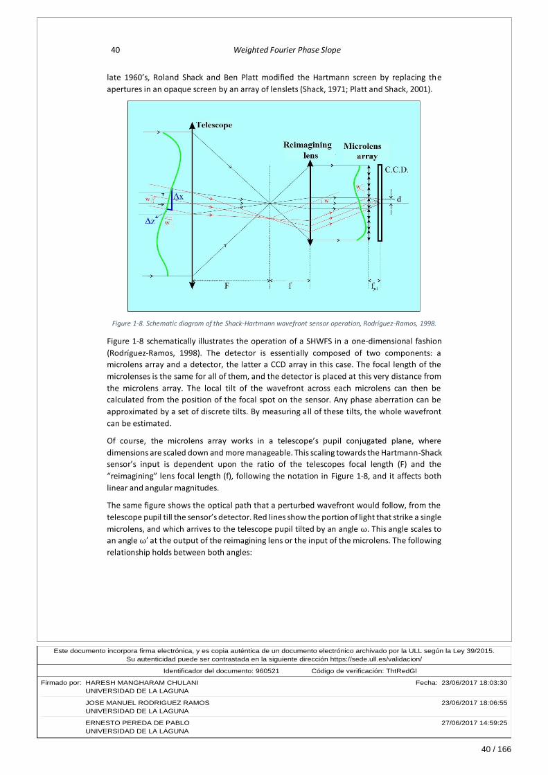
40 / 166
Este documento incorpora firma electrónica, y es copia auténtica de un documento electrónico archivado por la ULL según la Ley 39/2015.Su autenticidad puede ser contrastada en la siguiente dirección https://sede.ull.es/validacion/
Identificador del documento: 960521Código de verificación: ThtRedGl
Firmado por: HARESH MANGHARAM CHULANI Fecha: 23/06/2017 18:03:30UNIVERSIDAD DE LA LAGUNA
JOSE MANUEL RODRIGUEZ RAMOS 23/06/2017 18:06:55UNIVERSIDAD DE LA LAGUNA
ERNESTO PEREDA DE PABLO 27/06/2017 14:59:25UNIVERSIDAD DE LA LAGUNA
40 Weighted Fourier Phase Slope
late 1960’s, Roland Shack and Ben Platt modified the Hartmann screen by replacing the
apertures in an opaque screen by an array of lenslets (Shack, 1971; Platt and Shack, 2001).
Figure 1-8. Schematic diagram of the Shack-Hartmann wavefront sensor operation, Rodríguez-Ramos, 1998.
Figure 1-8 schematically illustrates the operation of a SHWFS in a one-dimensional fashion
(Rodríguez-Ramos, 1998). The detector is essentially composed of two components: a
microlens array and a detector, the latter a CCD array in this case. The focal length of the
microlenses is the same for all of them, and the detector is placed at this very distance from
the microlens array. The local tilt of the wavefront across each microlens can then be
calculated from the position of the focal spot on the sensor. Any phase aberration can be
approximated by a set of discrete tilts. By measuring all of these tilts, the whole wavefront
can be estimated.
Of course, the microlens array works in a telescope’s pupil conjugated plane, where
dimensions are scaled down and more manageable. This scaling towards the Hartmann-Shack
sensor’s input is dependent upon the ratio of the telescopes focal length (F) and the
“reimagining” lens focal length (f), following the notation in Figure 1-8, and it affects both
linear and angular magnitudes.
The same figure shows the optical path that a perturbed wavefront would follow, from the
telescope pupil till the sensor’s detector. Red lines show the portion of light that strike a single
microlens, and which arrives to the telescope pupil tilted by an angle ω. This angle scales to
an angle ω’at the output of the reimagining lens or the input of the microlens. The following
relationship holds between both angles:

41 / 166
Este documento incorpora firma electrónica, y es copia auténtica de un documento electrónico archivado por la ULL según la Ley 39/2015.Su autenticidad puede ser contrastada en la siguiente dirección https://sede.ull.es/validacion/
Identificador del documento: 960521Código de verificación: ThtRedGl
Firmado por: HARESH MANGHARAM CHULANI Fecha: 23/06/2017 18:03:30UNIVERSIDAD DE LA LAGUNA
JOSE MANUEL RODRIGUEZ RAMOS 23/06/2017 18:06:55UNIVERSIDAD DE LA LAGUNA
ERNESTO PEREDA DE PABLO 27/06/2017 14:59:25UNIVERSIDAD DE LA LAGUNA
Chapter 1. Atmospheric turbulence and adaptive optics 41
tan𝜔
tan𝜔′=𝑓
𝐹 [Eq. 1-11]
Note that angle ω is produced by a linear wavefront displacement Δz along the wavefront
optical axis z and across the subaperture width Δx, so for small angles, tan𝜔 = Δ𝑧 Δ𝑥⁄ . Also,
the spot displacement in the detector d is a consequence of wavefront angle of arrival ω’at the microlens, and so tan 𝜔′ = 𝑑 𝑓𝜇𝑙⁄ , where 𝑓𝜇𝑙 is the microlens focal length. Therefore, there
is relationship between the wavefront displacement at the system’s pupil Δz and the spot
displacement at the detector d which can be expressed as:
Δ𝑧
Δ𝑥=𝑓
𝐹
𝑑
𝑓𝜇𝑙 [Eq. 1-12]
Δz is a wavefront displacement measured in linear units. Here the variable 𝜙 is introduced as
the wavefront measured in radians, so that Δ𝜙 = (2𝜋 𝜆⁄ )Δ𝑧. Also, displacement d is
measured in linear units and can be expressed as the product of the displacement in pixels d’
and the pixel size dpix, finally leading to an expression that relates wavefront peak to valley
displacement Δϕ across the subaperture, in radians, to pixel displacement d’ of the spot:
Δϕ
Δ𝑥= [2𝜋
𝜆
𝑓
𝐹
𝑑𝑝𝑖𝑥𝑓𝜇𝑙] 𝑑′ [Eq. 1-13]
where all the terms into brackets are constants related to the system and sensor geometries.
1.3.2. Image processing and phase recovery at the SHWFS
It is clear from expression [Eq. 1-13] that the SHWFS senses phase gradient at every
subaperture and, consequently, in the whole aperture of the system. This statement relies on
the adequate measurement of the displacement of the spots at the detector. The normal
procedure to determine the spots’ displacements is to assign a certain portion of pixels of the
detector to each spot (and that portion will determine the FoV of the sensor) and compute
through some centroiding method the position of the spot in its assigned portion. This
position will be compared to a reference position measured, for example, by illuminating the
sensor with a plane wavefront. Point 1.4 is a review of the most employed centroiding
methods in a SHWFS.
Wavefront phase reconstruction at the whole system’s aperture is obtained from the
measurements of the 2N2 average phase slopes at the array of N2 subapertures. That is, in
each subaperture a pair of gradients are measured, one in each orthogonal axis. This implies
approximating the phase wavefront at the subaperture level to a plane, which is tilted
according to the estimated gradients. A phase recovery method is applied then to all the
measurements globally to obtain the whole aperture’s phase.
These methods are classified in two big groups:
Zonal methods, in which the phase at any point in the aperture is a function of the
phase and phase slope estimations at neighbour points.

42 / 166
Este documento incorpora firma electrónica, y es copia auténtica de un documento electrónico archivado por la ULL según la Ley 39/2015.Su autenticidad puede ser contrastada en la siguiente dirección https://sede.ull.es/validacion/
Identificador del documento: 960521Código de verificación: ThtRedGl
Firmado por: HARESH MANGHARAM CHULANI Fecha: 23/06/2017 18:03:30UNIVERSIDAD DE LA LAGUNA
JOSE MANUEL RODRIGUEZ RAMOS 23/06/2017 18:06:55UNIVERSIDAD DE LA LAGUNA
ERNESTO PEREDA DE PABLO 27/06/2017 14:59:25UNIVERSIDAD DE LA LAGUNA
42 Weighted Fourier Phase Slope
Modal methods, in which the phase is expressed as a linear combination of a set of
functions, which are orthogonal in the aperture. Zernike functions are the most
employed for circular apertures (see point 1.3.2.2).
Chapter 5 of the present work consists of a set of simulation tests performed over the whole
aperture of the SHWFS. For this purpose, the Object Oriented Matlab Adaptive Optics toolbox
(OOMAO, Conan and Correia, 2014) has been utilized. Here, some of the phase recovery
methods implemented in the toolbox and used in the tests are seen in detail.
1.3.2.1. Zonal methods for phase recovery
The starting point is a geometry consisting of phase gradients measured at certain points, and
phase points where the phase is to be estimated. Figure 1-9 (Herrmann, 1980) shows a
geometry that relates measured gradients and estimated phase points locations. Basically,
gradient is considered to be measured at the subaperture centres, and phase is estimated at
the corners of the subapertures. This geometry is called Fried geometry (Fried, 1977) and is
the one employed in the OOMAO toolbox.
Figure 1-9. Fried geometry with corresponding ‘A’ matrices in a SHWFS as depicted in Herrmann, 1980.
Figure 1-9 shows a simple case of 2 x 2 subapertures, and so 8 measured gradients and 9
points where to estimate phase. It also shows the A matrix that relates gradients to phases
for this particular case, according to the following expression (Herrman, 1980):
Δϕ = 𝐴ϕ [Eq. 1-14]
where Δϕ is a column vector of measured average phase gradients in both axes of each
subaperture and ϕ is a column vector of phases in the corners of the subapertures. Matrix A
has a deficiency in rank of 2 for Fried geometry. It is possible to define a reduced A matrix,
called Ar in Figure 1-9, by equalling phase at points 8 and 9 to zero. Alternatively, two
equations can be added to the system by imposing constraints to the sum of paired numbered
phases and the sum of odd numbered phases, resulting in the extended matrix Ae. Both Ar
and Ae are full rank and they lead to no indetermination when obtaining phases from
gradients.

43 / 166
Este documento incorpora firma electrónica, y es copia auténtica de un documento electrónico archivado por la ULL según la Ley 39/2015.Su autenticidad puede ser contrastada en la siguiente dirección https://sede.ull.es/validacion/
Identificador del documento: 960521Código de verificación: ThtRedGl
Firmado por: HARESH MANGHARAM CHULANI Fecha: 23/06/2017 18:03:30UNIVERSIDAD DE LA LAGUNA
JOSE MANUEL RODRIGUEZ RAMOS 23/06/2017 18:06:55UNIVERSIDAD DE LA LAGUNA
ERNESTO PEREDA DE PABLO 27/06/2017 14:59:25UNIVERSIDAD DE LA LAGUNA
Chapter 1. Atmospheric turbulence and adaptive optics 43
Least-squares minimum norm solution is the first zonal phase recovery method to be
proposed (Fried, 1977; Hudgin, 1977; Herrmann, 1980). OOMAO calls it Direct Fitting. It is
based on the generalized Moore-Penrose matrix inversion, and can be expressed as:
ϕ̂𝐿𝑆𝑀𝑁 = 𝐴+ Δϕ [Eq. 1-15]
with 𝐴+being the generalized inverse or pseudo-inverse of matrix 𝐴, and ϕ̂𝐿𝑆𝑀𝑁 the estimated
phases from the measured gradients Δϕ.
Linear Minimum Mean Square Error (LMMSE)
Minimum Mean Square Error (MMSE) estimator is a Bayesian estimation method which
minimizes the mean square error of the fitted values of the variable to be estimated, and it is
given by the posterior mean of the parameter to be estimated. In the case being dealt with
here, it would be expressed as:
ϕ̂𝑀𝑀𝑆𝐸 = ⟨ϕ Δϕ⁄ ⟩ [Eq. 1-16]
MMSE becomes the linear MMSE or LMMSE when a linear dependency of the parameter to
be estimated upon the measured variable is assumed. In our case, and taking into account
that phase and phase gradients are zero mean variables, the LMMSE estimator of the phase
would be:
ϕ̂𝐿𝑀𝑀𝑆𝐸 = 𝐶ϕΔϕ𝐶Δϕ−1Δϕ [Eq. 1-17]
where 𝐶ϕΔϕ is the cross-covariance matrix between ϕ and Δϕ, and 𝐶Δϕ is the auto-covariance
matrix of Δϕ.
This is a second choice of zonal phase recovery method implemented in the OOMAO toolbox.
1.3.2.2. Modal methods for phase recovery. Zernike functions.
It is sometimes useful to represent a phase by the coefficients of an expansion in a set of basic
functions. Zernike polynomials are very conveniently used because of their simplicity and
physical meaning. This could be expressed as:
𝜙(𝑥, 𝑦) =∑𝑐𝑗 𝑍𝑗(𝑥,𝑦) [Eq. 1-18]
x and y being the coordinates where phase ϕ and set of Zernike functions 𝑍𝑗 are defined, and
𝑐𝑗 are the coefficients of the expansion.
The definition of Zernike functions for polar coordinates can be found in Noll, 1976. For n the
radial order and m the azimuthal order, both nonnegative integers fulfilling n≥m and n-m

44 / 166
Este documento incorpora firma electrónica, y es copia auténtica de un documento electrónico archivado por la ULL según la Ley 39/2015.Su autenticidad puede ser contrastada en la siguiente dirección https://sede.ull.es/validacion/
Identificador del documento: 960521Código de verificación: ThtRedGl
Firmado por: HARESH MANGHARAM CHULANI Fecha: 23/06/2017 18:03:30UNIVERSIDAD DE LA LAGUNA
JOSE MANUEL RODRIGUEZ RAMOS 23/06/2017 18:06:55UNIVERSIDAD DE LA LAGUNA
ERNESTO PEREDA DE PABLO 27/06/2017 14:59:25UNIVERSIDAD DE LA LAGUNA
44 Weighted Fourier Phase Slope
even, a pair of even and odd Zernike functions are defined for m≠0 or a single function for
m=0:
𝑍𝑛𝑚(𝜌,𝜃) = √2(𝑛 + 1)𝑅𝑛
𝑚(𝜌) cos(𝑚𝜃)
𝑍𝑛−𝑚(𝜌, 𝜃) = √2(𝑛 + 1)𝑅𝑛
𝑚(𝜌)sin(𝑚𝜃)}𝑚 ≠ 0
𝑍𝑛𝑚(𝜌, 𝜃) = √(𝑛 + 1)𝑅𝑛
0(𝜌), 𝑚 = 0
[Eq. 1-19]
with 𝜌 the normalized radial distance 0 ≤ 𝜌 ≤ 1, and 𝜃 the azimuthal angle. The radial
polynomials 𝑅𝑛𝑚(𝜌) are defined as:
𝑅𝑛𝑚(𝜌) = ∑
(−1)𝑠(𝑛 − 𝑠)!
𝑠! [𝑛 + 𝑚2
− 𝑠] ! [𝑛 − 𝑚2
− 𝑠] !𝜌𝑛−2𝑠
(𝑛−𝑚)/2
𝑠=0
[Eq. 1-20]
Noll (1976) mapped the m and n indexes into a single index j, with the following rule: even
Zernike functions -with azimuthal part cos(𝑚𝜃)- receive even indexes j; odd Zernike functions
-with azimuthal part sin(𝑚𝜃)- receive odd indexes j; lower n values receive lower j; and within
a given n, lower values of m receive lower j.
So, any wavefront phase 𝜙(𝑟, 𝜃) defined in a circular aperture with radius R as a function of
radial coordinate 𝑟, 0 ≤ 𝑟 ≤ 𝑅, and azimuthal coordinate 𝜃, can be expressed as:
𝜙(𝑟, 𝜃) = 𝜙(𝑅𝜌, 𝜃) = ∑𝑐𝑗𝑍𝑗(𝜌, 𝜃)
𝑗
[Eq. 1-21]
Zernike functions correspond to classic optical aberrations such as tilt, defocus, astigmatism,
coma, spherical aberration, distortion, field curvature, etc. The coefficients 𝑐𝑗 give and idea
of the dominant aberrations in the propagation medium. Zernike modal phase recovery
means estimating such Zernike coefficients. A vectorised expression from [Eq. 1-21] would
be:
𝜙 = 𝑍𝑐 [Eq. 1-22]
with 𝜙 a column vector of phases at the discrete point of estimation, c a column vector of
coefficients and Z a matrix with as many columns as Zernike functions are used in the
expansion and as many rows as evaluation coordinates of the same. Substituting 𝜙 in
equation [Eq. 1-14] by its value in [Eq. 1-22], a relationship between measured phase
gradients and Zernike coefficients is obtained:
Δϕ = (𝐴𝑍)𝑐 [Eq. 1-23]
Product of matrixes 𝐴𝑍 is equivalent to computing the phase difference of each Zernike
function across the subapertures of the sensor. The OOMAO toolbox computes this matrix in

45 / 166
Este documento incorpora firma electrónica, y es copia auténtica de un documento electrónico archivado por la ULL según la Ley 39/2015.Su autenticidad puede ser contrastada en la siguiente dirección https://sede.ull.es/validacion/
Identificador del documento: 960521Código de verificación: ThtRedGl
Firmado por: HARESH MANGHARAM CHULANI Fecha: 23/06/2017 18:03:30UNIVERSIDAD DE LA LAGUNA
JOSE MANUEL RODRIGUEZ RAMOS 23/06/2017 18:06:55UNIVERSIDAD DE LA LAGUNA
ERNESTO PEREDA DE PABLO 27/06/2017 14:59:25UNIVERSIDAD DE LA LAGUNA
Chapter 1. Atmospheric turbulence and adaptive optics 45
a recursive manner (Stephenson P., 2014, for example). So, a first option of modal phase
recovery offered by OOMAO is inverting the above expression [Eq. 1-23] in a minimum least
squares sense to obtain a direct relationship between Zernike coefficients c and measured
gradients Δϕ:
�̂�𝑔 = (𝐴𝑍)+ Δϕ [Eq. 1-24]
A second option would be a two steps option. First, a zonal phase recovery method is applied
to estimate the phases 𝜙, for example by LSMN estimation; second, coefficients c are
estimated by solving the set of equations in expression [Eq. 1-22] in a least squares sense:
�̂� = 𝑍+𝐴+Δϕ [Eq. 1-25]
Expressions [Eq. 1-24] and [Eq. 1-25] do not give the same results. In the first option, a least
squares fit gives the minimum variance of the gradients, and hence the subscript g, whereas
the second option gives a minimum variance of the phase (Herrmann, 1980).
1.4. Centroiding methods in a SHWFS
When a light wavefront strikes a SHWFS, a spots matrix is registered at the detector as a
consequence of light going through the microlens array. Each spot is displaced, with respect
to the plane wavefront case, a distance proportional to the average wavefront gradient as
expressed in equation [Eq. 1-13]. Methods have been devised that deal globally with the
matrix spots and obtain the phase gradient by spatial demodulation of the whole image in
the detector (Carmon and Ribak, 2003; Talmi and Ribak, 2004; Sarver et al, 2006; Lukin et al,
2010). Nevertheless, the most common approach is the independent treatment of each
subaperture, consisting of estimating the displacement of the corresponding spot at the
detector, followed by a phase recovery method that deals globally with the gradients matrix,
such as those described in point 1.3.2. The methods employed to estimate the displacement
of each spot in its assigned portion of detector are generally called centroiding methods, both
when absolute displacement is estimated and when the displacement is relative to a
reference spot.
It is convenient to clarify that two possible definitions for a circular subaperture phase tilt can
be found (see Tyler, 1994, for example). One is the G-tilt, which is the average phase gradient
over the aperture. The other one is the Z-tilt, or Zernike tilt, and is the tilt of the best planar
approximation of the phase in a least squares error sense. For symmetric spots, both tilts
coincide. However, when asymmetric phase modes dominate, both tilts differ. Centre of
gravity based centroiding methods actually estimate G-tilt, whereas when minimizing phase
estimation error or maximizing Strehl ratio is desired, a Z-tilt estimation in the subperture
would be preferred.
46 / 166
Este documento incorpora firma electrónica, y es copia auténtica de un documento electrónico archivado por la ULL según la Ley 39/2015.Su autenticidad puede ser contrastada en la siguiente dirección https://sede.ull.es/validacion/
Identificador del documento: 960521Código de verificación: ThtRedGl
Firmado por: HARESH MANGHARAM CHULANI Fecha: 23/06/2017 18:03:30UNIVERSIDAD DE LA LAGUNA
JOSE MANUEL RODRIGUEZ RAMOS 23/06/2017 18:06:55UNIVERSIDAD DE LA LAGUNA
ERNESTO PEREDA DE PABLO 27/06/2017 14:59:25UNIVERSIDAD DE LA LAGUNA
46 Weighted Fourier Phase Slope
Three are the most known and favourite centroiding method families which are foreseen to
be employed in ELT’s (Thomas et al, 2006; Gradatour et al, 2010; Lardière et al, 2010): centre
of gravity (CoG), cross-correlation (CC) and matched filter (MF).
1.4.1. Centre of Gravity (CoG) based methods
The centre of gravity algorithm applies to each spot image I, defined across the x-horizontal
coordinate and y-vertical coordinate, the following function:
𝑐𝑜𝑔(𝐼) = (∑𝑥𝐼(𝑥, 𝑦)
𝑥,𝑦
∑𝐼(𝑥, 𝑦)
𝑥,𝑦
⁄ ,∑𝑦𝐼(𝑥, 𝑦)
𝑥,𝑦
∑𝐼(𝑥, 𝑦)
𝑥,𝑦
⁄ ) [Eq. 1-26]
In the absence of noise, it is a direct estimator of the average phase gradient at the aperture
or G-tilt. It is a linear estimator for small spot’s displacements, such as in closed loop system’s
operation. However, it is very much affected by spot’s truncation and by detector’s noise
when a large FoV, implying more detector’s pixels into play, and high dynamic range are
required, such as in open loop operation. The following are variations to the simple CoG that
intend to improve its robustness against these effects.
1.4.1.1. Thresholded centre of gravity (TCoG)
It applies a threshold T to the image I, and only those pixels with a brighter intensity than T
are taken into account for CoG computation, according to the following expression:
𝑡𝑐𝑜𝑔(𝐼) =
(
∑ 𝑥[𝐼(𝑥, 𝑦) − 𝑇]
𝑥,𝑦 𝐼⁄ ≥𝑇
∑ [𝐼(𝑥, 𝑦) − 𝑇]
𝑥,𝑦 𝐼⁄ ≥𝑇
⁄ ,
∑ 𝑦[𝐼(𝑥, 𝑦) − 𝑇]
𝑥,𝑦 𝐼⁄ ≥𝑇
∑ [𝐼(𝑥, 𝑦) − 𝑇]
𝑥,𝑦 𝐼⁄ ≥𝑇
⁄
)
[Eq. 1-27]
Threshold T is normally a fraction of the spot’s maximum intensity, with a lower bound which
depends on the detector’s noise. It is preferably determined by optimization, since
thresholding is itself a source of nonlinear noise (Arines and Ares, 2002).
1.4.1.2. Weighted centre of gravity (WCoG)
It applies a weight W to the image I before centroiding, and so its formulation is:
𝑤𝑐𝑜𝑔(𝐼,𝑊) = 𝑐𝑜𝑔(𝐼×𝑊) [Eq. 1-28]
Weight W is normally a Gaussian centred at the image’s centre, intending to give more weight
to brighter pixels and to attenuate noisy pixels, for an assumed centred spot. So WCoG
method is adequate for small displacements in the spot, as in closed loop operation in XAO
systems (Nicolle, 2004; Fusco, 2004). It becomes nonlinear for big displacements as the spot’s
shape gets distorted, and needs careful calibration and linearization to compensate spot’s
distortion and gain dynamic range (Lardière et al, 2010). Optimization of the width of the
47 / 166
Este documento incorpora firma electrónica, y es copia auténtica de un documento electrónico archivado por la ULL según la Ley 39/2015.Su autenticidad puede ser contrastada en la siguiente dirección https://sede.ull.es/validacion/
Identificador del documento: 960521Código de verificación: ThtRedGl
Firmado por: HARESH MANGHARAM CHULANI Fecha: 23/06/2017 18:03:30UNIVERSIDAD DE LA LAGUNA
JOSE MANUEL RODRIGUEZ RAMOS 23/06/2017 18:06:55UNIVERSIDAD DE LA LAGUNA
ERNESTO PEREDA DE PABLO 27/06/2017 14:59:25UNIVERSIDAD DE LA LAGUNA
Chapter 1. Atmospheric turbulence and adaptive optics 47
Gaussian weight W is convenient in this sense, to get a good compromise between noise
rejection and linearity.
Some variations of this algorithm have been proposed that intend to gain in dynamic range:
IWC or Intensity Weighted Centroiding, in which weights are the pixel intensities themselves,
and IWCoG, for Iteratively Weighted Centre of Gravity, where weights are iteratively
displaced to the measured spot position (Vyas, Roopashree and Prasad, 2009a).
1.4.1.3. Quad Cell (QC)
Quad Cell is the particular case of a CoG with only 2 x 2 pixels or cells. Numbering those pixels
from 1 to 4, starting upward to the left and in anti-clockwise direction, its formula would be:
𝑞𝑐(𝐼) = (1
𝐺𝑥
𝐼1 + 𝐼2 − 𝐼3 − 𝐼4𝐼1 + 𝐼2 + 𝐼3 + 𝐼4
,1
𝐺𝑦
𝐼1 − 𝐼2 + 𝐼3 − 𝐼4𝐼1 + 𝐼2 + 𝐼3 + 𝐼4
) [Eq. 1-29]
This method is very sensitive to spot’s shape variations. 𝐺𝑥and 𝐺𝑦intend to compensate for
gain variations in x and y axis due to different spot’s elongation. It is a preferred method for
very low light flux level, but it is only suitable for closed loop operation and needs calibration
and compensation for its nonlinearities.
1.4.2. Cross-Correlation (CC) method
Cross-correlation method applied for extended objects can be applied also to point-like
sources (Poyneer et al, 2004). The cross-correlation between the snapshot or live image I and
a reference image I0 is computed, and a correlation figure is obtained. Centroid of the
correlation figure is an estimation of displacement between live and reference images. For
subpixel accuracy, this centroid can be computed with a CoG, habitually thresholded, or with
curve fitting methods. Correlation can be computed in the image domain, but for
computational cost reasons, it is preferably performed in the Fourier domain (Sidick et al,
2008).
It has been reported (Poyneer et al, 2004; Thomas et al, 2006; Gradatour et al, 2010; Lardière
et al, 2010) that CC is more robust than CoG based methods against detector noise; it is more
linear allowing for a higher dynamic range, and it is less impacted by variations in the spot
shape. The cons are a much higher computational cost and the need for a proper reference
selection. Nonetheless, at high light flux level both CC and CoG methods perform similarly and
are limited by photonic noise.
Recently, CC performance in the RAVEN MOAO system for the Subaru telescope for natural
and laser guide stars has been reported (Andersen et al, 2014). An increase in 0.5 to 1 in
limiting magnitude is predicted at a cost of a decrease of frequency system from 250 to 150
Hz, so it CC is particularly suited to very low light flux levels. They report CC is more robust
than other methods against spot undersampling and large FoV’s.

48 / 166
Este documento incorpora firma electrónica, y es copia auténtica de un documento electrónico archivado por la ULL según la Ley 39/2015.Su autenticidad puede ser contrastada en la siguiente dirección https://sede.ull.es/validacion/
Identificador del documento: 960521Código de verificación: ThtRedGl
Firmado por: HARESH MANGHARAM CHULANI Fecha: 23/06/2017 18:03:30UNIVERSIDAD DE LA LAGUNA
JOSE MANUEL RODRIGUEZ RAMOS 23/06/2017 18:06:55UNIVERSIDAD DE LA LAGUNA
ERNESTO PEREDA DE PABLO 27/06/2017 14:59:25UNIVERSIDAD DE LA LAGUNA
48 Weighted Fourier Phase Slope
1.4.3. Matched Filter (MF) method2
Matched Filter method is based on a first order approximation of the Taylor expansion of the
spot’s image intensity I as a function of spot displacement with respect to a reference spot’s
image I0 (Lardière et al, 2010):
𝐼 = 𝐼0 + (𝑑𝑥 − 𝑑0𝑥)𝜕𝐼
𝜕𝑑𝑥+ (𝑑𝑦 − 𝑑0𝑦)
𝜕𝐼
𝜕𝑑𝑦 [Eq. 1-30]
with (𝑑𝑥,𝑑𝑦) the coordinates of the live spot and (𝑑0𝑥,𝑑0𝑦) the coordinates of the reference
spot. This Taylor expansion is only valid if the current image I is a shifted copy of the reference
image I0 and if the shift is of a very small amount (a fraction of a pixel). [Eq. 1-30] can be
expressed for each subaperture in a matrix notation as:
𝐼 − 𝐼0 = 𝐺𝑚𝑓(𝑑 − 𝑑0) [Eq. 1-31]
with 𝐺𝑚𝑓the matched filter gain matrix composed of the pixel intensity derivatives for both
x- and y-directions. [Eq. 1-31] can be solved for each lenslet slope d as:
�̂�𝑚𝑓 = 𝑅(𝐼 − 𝐼0) + 𝑑0 [Eq. 1-32]
with R the pseudo-inverse of the matrix 𝐺𝑚𝑓 .
MF method is suited for low flux level. It requires proper reference selection and refreshment;
and a correct calibration against the updated reference.
2 Some authors use the terms Matched Filter and Cross-Correlation interchangeably (Leroux and Dainty, 2010, for example). It is not the case in the present work.

49 / 166
Este documento incorpora firma electrónica, y es copia auténtica de un documento electrónico archivado por la ULL según la Ley 39/2015.Su autenticidad puede ser contrastada en la siguiente dirección https://sede.ull.es/validacion/
Identificador del documento: 960521Código de verificación: ThtRedGl
Firmado por: HARESH MANGHARAM CHULANI Fecha: 23/06/2017 18:03:30UNIVERSIDAD DE LA LAGUNA
JOSE MANUEL RODRIGUEZ RAMOS 23/06/2017 18:06:55UNIVERSIDAD DE LA LAGUNA
ERNESTO PEREDA DE PABLO 27/06/2017 14:59:25UNIVERSIDAD DE LA LAGUNA
Chapter 2. Objective of the present work
2.1. Motivation of the work
The centroiding method in a Shack Hartmann wavefront sensor plays a crucial role in
determining the robustness of the sensor against the measurement noise described in point
1.2.2.2. With the recent interest in MOAO systems, in which turbulence is sensed and
compensated for in open loop, the requirement of balancing sensitivity respect to light flux
level with a high dynamic range has become a very desirable trait in wavefront sensors.
Moreover, a very low light level situation calls for a configuration with high subaperture size
to Fried parameter ratio and, hence, a centroiding method which is robust against high order
aberrations in the spot is required. All this should be combined with a fast algorithm with low
computational cost in order to keep the temporal error described in point 1.2.2.4 as low as
possible.
The success of the CoG based methods is understandable from the point of view of simplicity
and low hardware resources requirement. However, they are prone to noise when many
pixels per subaperture come into play, such as when a large dynamic range or field of view is
required. WCoG and QC are adaptations of pure CoG that make the sensor more sensitive,
but at the cost of lowering the dynamic range, making them suitable only for closed loop
system operation. TCoG is perhaps the CoG derived method which best balances sensitivity
and dynamic range requirement; yet, threshold cannot be kept high in low light level
conditions, and non-Gaussian type of noise such as CIC noise in Electron Multiplying CCD’s
(EMCCD’s) cannot be fully managed with a simple threshold.
Hardware speed and processing capabilities are in continuous growth. Modern GPU’s
(Graphical Processor Units), which were in principle thought for commercial applications with
a high computational demand due to video processing, such as 3D games, are taken
advantage of in scientific applications where the high computational load is parallelizable.
Another hardware processing component which is parallel in nature is the FPGA (Field
Programmable Gate Array). It is programmable hardware, and was in principle thought of as
a digital electronics prototyping component. More recently, it has been used for scientific
parallel demanding computation, such as computing the 2D-FFT (bi-dimensional Fast Fourier

50 / 166
Este documento incorpora firma electrónica, y es copia auténtica de un documento electrónico archivado por la ULL según la Ley 39/2015.Su autenticidad puede ser contrastada en la siguiente dirección https://sede.ull.es/validacion/
Identificador del documento: 960521Código de verificación: ThtRedGl
Firmado por: HARESH MANGHARAM CHULANI Fecha: 23/06/2017 18:03:30UNIVERSIDAD DE LA LAGUNA
JOSE MANUEL RODRIGUEZ RAMOS 23/06/2017 18:06:55UNIVERSIDAD DE LA LAGUNA
ERNESTO PEREDA DE PABLO 27/06/2017 14:59:25UNIVERSIDAD DE LA LAGUNA
50 Weighted Fourier Phase Slope
Transform) or in a full-FPGA AO system (Rodríguez-Ramos J.M et al, 2008; Chulani H.M. et al,
2016). Processing components such as GPU’s and FPGA’s allow for centroiding methods with
a certain computational complexity to be implemented in a SHWFS and still its computational
latency be negligible in comparison to the latency due to other required operations such as
light integration, image read and DM shape change.
Some authors have proposed shifting from the image domain to transformed domains where
denoising filters are easier to apply. In this sense, the Zernike expansion of the image has
been proposed (Vyas, Roopashree and Prasad, 2009b), followed even by feature extraction
and Gaussian pattern matching techniques (Vyas, Roopashree and Prasad, 2010). A
somewhat similar method is the Gram-Charlier expansion of the Gaussian fit of the image and
subsequent filtering proposed by Ruggiu, Solomon and Loos (1998).
The Fourier transform of a discrete image Ixy is its expansion into a base of discrete
exponentials, according to the expression (Oppenheim and Schafer, 1989)
𝕀(𝜔𝑥, 𝜔𝑦) = ℱ{𝐼𝑥𝑦}|𝜔𝑥 ,𝜔𝑦=∑∑𝐼𝑥𝑦𝑒
−𝑗𝜔𝑥𝑥𝑒−𝑗𝜔𝑦𝑦
𝑦𝑥
[Eq. 2-1]
with ℱ{·} the Fourier transform operation, 𝜔𝑥 = 2𝜋𝑓𝑥, 𝜔𝑦 = 2𝜋𝑓𝑦 , 𝑓𝑥 and 𝑓𝑦 the spatial
frequencies in the x- and y-axis, respectively, and −𝜋 ≤ 𝜔𝑥 ≤ 𝜋, −𝜋 ≤ 𝜔𝑦 ≤ 𝜋, or,
alternatively, 𝜔𝑥and 𝜔𝑦ranging any interval of length 2𝜋, since the Fourier transform is
periodic in both axes with period 2𝜋.
Fast algorithms have been developed that compute a discrete version of the Fourier
transform of a discrete signal (Fast Fourier Transform, abbreviated FFT). Besides, many
operations in the image domain have their counterparts in the Fourier domain. Cross-
correlation in the image domain, for example, becomes a multiplication (and conjugation of
one of the terms) in the Fourier domain. Furthermore, displacement in the image domain is
equivalent to a planar phase addition in the Fourier domain ([Eq. 2-2]). This has led to the CC
centroiding method being completely calculated in the Fourier domain, as described in Sidick
et al, 2008. After multiplication of the image’s Fourier transform by the reference’s Fourier
conjugate, a least squares fit is applied to the phase of the product to compute its slope, and
so, the displacement of the correlation figure.
The relationship between image displacement and Fourier phase slope can be easily derived
from [Eq. 2-1] and expressed as
ℱ{𝐼𝑥𝑦(𝑥 − 𝑥0, 𝑦 − 𝑦0)}|𝜔𝑥 ,𝜔𝑦= 𝕀(𝜔𝑥 , 𝜔𝑦)𝑒
−𝑗𝜔𝑥𝑥0𝑒−𝑗𝜔𝑦𝑦0 [Eq. 2-2]
This is represented in a one-dimensional simplification in Figure 2-1 (Li, Huang and Gong,
2014). Based in this very principle, professor J. P. Fillard and his group at the Université de
Montpellier proposed a method they called Fourier Phase Shift (FPS) as an alternative to the
CoG centroiding method (Fillard, 1992; Fillard et al, 1993), back in the 90’s. It consisted of
applying a least squares planar fit to the phase of the image’s Fourier transform to obtain its
slope, thus estimating what he called a best symmetric centre of the spot, since a plane
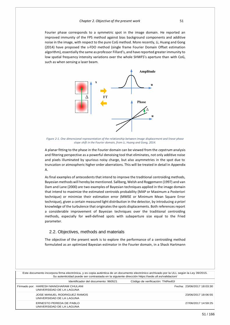
51 / 166
Este documento incorpora firma electrónica, y es copia auténtica de un documento electrónico archivado por la ULL según la Ley 39/2015.Su autenticidad puede ser contrastada en la siguiente dirección https://sede.ull.es/validacion/
Identificador del documento: 960521Código de verificación: ThtRedGl
Firmado por: HARESH MANGHARAM CHULANI Fecha: 23/06/2017 18:03:30UNIVERSIDAD DE LA LAGUNA
JOSE MANUEL RODRIGUEZ RAMOS 23/06/2017 18:06:55UNIVERSIDAD DE LA LAGUNA
ERNESTO PEREDA DE PABLO 27/06/2017 14:59:25UNIVERSIDAD DE LA LAGUNA
Chapter 2. Objective of the present work 51
Fourier phase corresponds to a symmetric spot in the image domain. He reported an
improved immunity of the FPS method against bias background components and additive
noise in the image, with respect to the pure CoG method. More recently, Li, Huang and Gong
(2014) have proposed the s-FDO method (single frame Fourier Domain Offset estimation
algorithm), essentially the same as professor Fillard’s, and have reported greater immunity to
low spatial frequency intensity variations over the whole SHWFS’s aperture than with CoG,
such as when sensing a laser beam.
Figure 2-1. One dimensional representation of the relationship between image displacement and linear phase slope shift in the Fourier domain, from Li, Huang and Gong, 2014.
A planar fitting to the phase in the Fourier domain can be viewed from the cepstrum analysis
and filtering perspective as a powerful denoising tool that eliminates, not only additive noise
and pixels illuminated by spurious noisy charge, but also asymmetries in the spot due to
truncation or atmospheric higher order aberrations. This will be treated in detail in Appendix
A.
As final examples of antecedents that intend to improve the traditional centroiding methods,
Bayesian methods will hereby be mentioned. Sallberg, Welsh and Roggemann (1997) and van
Dam and Lane (2000) are two examples of Bayesian techniques applied in the image domain
that intend to maximize the estimated centroids probability (MAP or Maximum a Posteriori
technique) or minimize their estimation error (MMSE or Minimum Mean Square Error
technique), given a certain measured light distribution in the detector, by introducing a priori
knowledge of the turbulence that originates the spots displacements. Both references report
a considerable improvement of Bayesian techniques over the traditional centroiding
methods, especially for well-defined spots with subaperture size equal to the Fried
parameter.
2.2. Objectives, methods and materials
The objective of the present work is to explore the performance of a centroiding method
formulated as an optimized Bayesian estimator in the Fourier domain, in a Shack Hartmann

52 / 166
Este documento incorpora firma electrónica, y es copia auténtica de un documento electrónico archivado por la ULL según la Ley 39/2015.Su autenticidad puede ser contrastada en la siguiente dirección https://sede.ull.es/validacion/
Identificador del documento: 960521Código de verificación: ThtRedGl
Firmado por: HARESH MANGHARAM CHULANI Fecha: 23/06/2017 18:03:30UNIVERSIDAD DE LA LAGUNA
JOSE MANUEL RODRIGUEZ RAMOS 23/06/2017 18:06:55UNIVERSIDAD DE LA LAGUNA
ERNESTO PEREDA DE PABLO 27/06/2017 14:59:25UNIVERSIDAD DE LA LAGUNA
52 Weighted Fourier Phase Slope
wavefront sensor. The scope of the present work is limited to night time astronomical
adaptive optics applications, where a natural guide star is the sensing light source. This novel
algorithm’s mathematical expression will be derived, and its advantages and disadvantages
with respect to most utilized centroiding methods such as TCoG, WCoG and CC will be
determined, according to the following figures of merit:
Real time implementation feasibility. In that sense, the number of operations to be
performed in a system cycle per SHWFS subaperture and whole aperture will be
worked out and contrasted with the computational power of modern processors and
co-processors.
Balance between sensitivity and dynamic range. In that sense, the behaviour of the
centroiding method will be evaluated as a function of light flux level, detector noises
and required field of view for open and closed loop operation.
The effect of spot truncation due to a limited number of pixels (and hence, limited
field of view) in the sensor will be determined and compared with the behaviour of
the other centroiding methods.
Robustness against high order aberrations in the spot, more noticeable as the size of
the subaperture with respect to the Fried parameter increases, will be evaluated and
compared.
The proposed algorithm’s characteristics in terms of sensitivity, dynamic range and
robustness against spot’s deformation will be determined firstly at a subaperture level
through numerical simulation. MATLAB™3 software package will be used for this purpose.
Numerical simulations will then be extended to the whole SHWFS aperture with the aid of a
free open MATLAB toolbox called Object Oriented Matlab for Adaptive Optics toolbox
(OOMAO, Conan and Correia, 2014). The whole sensor’s behaviour with this new proposed
centroid method can be thus evaluated, and Strehl Ratio as well as Encircled Energy figures
due to measurement and fitting errors can be estimated.
Finally, the work done by the author for the EDiFiSE (Equalized and Diffraction limited Field
Spectrograph Experiment) project at the IAC (Instituto de Astrofísica de Canarias) has created
the opportunity of utilizing its adaptive optics setup at the optical laboratory facility of the
institute. This setup consists of a full-FPGA closed loop controlled SCAO system with a SHWFS
that comprises a microlens array and an EMCCD Andor Ixon+ detector of 128 by 128 pixels
(Chulani et al, 2016). It receives a perturbed light wavefront from the IACAT (IAC’s
Atmosphere and Telescope) ground support equipment (Moreno-Raso et al, 2010). Inside the
IACAT, Kolmogorov turbulence is emulated by phase plates with the appropriate refractive
index drawing, with five phase plates in total that emulate a different Fried parameter each,
and the possibility of combining up to three phase plates simultaneously in the optical bench.
The aperture and focal length characteristics of three different telescopes can also be
emulated; the 4,2 m William Herschel Telescope’s configuration will be selected. Light source
is intensity regulated.
3 MATLAB is a registered trademark of The Mathworks, Inc.

53 / 166
Este documento incorpora firma electrónica, y es copia auténtica de un documento electrónico archivado por la ULL según la Ley 39/2015.Su autenticidad puede ser contrastada en la siguiente dirección https://sede.ull.es/validacion/
Identificador del documento: 960521Código de verificación: ThtRedGl
Firmado por: HARESH MANGHARAM CHULANI Fecha: 23/06/2017 18:03:30UNIVERSIDAD DE LA LAGUNA
JOSE MANUEL RODRIGUEZ RAMOS 23/06/2017 18:06:55UNIVERSIDAD DE LA LAGUNA
ERNESTO PEREDA DE PABLO 27/06/2017 14:59:25UNIVERSIDAD DE LA LAGUNA
Chapter 2. Objective of the present work 53
The SHWFS will be utilized in this setup to acquire image sequences distorted by static
turbulent patterns, with different light fluxes and turbulence strengths, and without applying
any correction, so that dynamic range requirement at the wavefront sensor is high. Image
sequences will be processed offline with different centroiding algorithms and the wavefront
recovery error determined for each sequence and each algorithm. Applied static wavefront
perturbation is actually unknown, but can be estimated as an average of wavefront phases
recovered by the centroiding methods under study in a very bright light level situation. The
objective is to compare each algorithm’s characteristics of sensitivity, dynamic range and
robustness against spots deformation due to limited FoV and/or turbulence.
A previous step is the complete sensitivity, gain and noise characterization of the EMCCD
detector, in order to correctly estimate the flux level and SNR’s from the recorded images.

54 / 166
Este documento incorpora firma electrónica, y es copia auténtica de un documento electrónico archivado por la ULL según la Ley 39/2015.Su autenticidad puede ser contrastada en la siguiente dirección https://sede.ull.es/validacion/
Identificador del documento: 960521Código de verificación: ThtRedGl
Firmado por: HARESH MANGHARAM CHULANI Fecha: 23/06/2017 18:03:30UNIVERSIDAD DE LA LAGUNA
JOSE MANUEL RODRIGUEZ RAMOS 23/06/2017 18:06:55UNIVERSIDAD DE LA LAGUNA
ERNESTO PEREDA DE PABLO 27/06/2017 14:59:25UNIVERSIDAD DE LA LAGUNA
55 / 166
Este documento incorpora firma electrónica, y es copia auténtica de un documento electrónico archivado por la ULL según la Ley 39/2015.Su autenticidad puede ser contrastada en la siguiente dirección https://sede.ull.es/validacion/
Identificador del documento: 960521Código de verificación: ThtRedGl
Firmado por: HARESH MANGHARAM CHULANI Fecha: 23/06/2017 18:03:30UNIVERSIDAD DE LA LAGUNA
JOSE MANUEL RODRIGUEZ RAMOS 23/06/2017 18:06:55UNIVERSIDAD DE LA LAGUNA
ERNESTO PEREDA DE PABLO 27/06/2017 14:59:25UNIVERSIDAD DE LA LAGUNA
Chapter 3. The Weighted Fourier Phase Slope algorithm
This chapter presents the mathematical definition of the centroiding method under study in
this work. It has been given the name Weighted Fourier Phase Slope (abbreviated WFPS),
because it first calculates the slopes, or derivatives with respect to both spatial frequency
axes, of the image’s Fourier phase, and then averages these slopes with optimized weights in
order to obtain the centroid’s horizontal and vertical coordinates in the image domain . The
computational cost of such an algorithm is also presented, and contrasted with other known
algorithms.
This innovative centroiding method has been presented in the IEEE 12th Workshop on
Information Optics (Chulani and Rodríguez-Ramos, 2013) and has been accepted for
presentation at the 5th Adaptive Optics for Extremely Large Telescopes Conference (Chulani
and Rodríguez-Ramos, 2017).
3.1. Fourier Phase Slope
For a given SHWFS subaperture image 𝐼𝑥𝑦, its Fourier transform is
𝕀(𝜔𝑥, 𝜔𝑦) = ℱ{𝐼𝑥𝑦}|𝜔𝑥 ,𝜔𝑦=∑∑𝐼𝑥𝑦𝑒
−𝑗𝜔𝑥𝑥𝑒−𝑗𝜔𝑦𝑦
𝑦𝑥
[Eq. 3-1]
following the notation in [Eq. 2-1], and can be expressed as
𝕀(𝜔𝑥, 𝜔𝑦) = |𝕀(𝜔𝑥, 𝜔𝑦)|𝑒𝑗𝑎𝑟𝑔(𝕀(𝜔𝑥 ,𝜔𝑦)) [Eq. 3-2]
with |𝕀(𝜔𝑥, 𝜔𝑦)| and 𝑎𝑟𝑔 (𝕀(𝜔𝑥, 𝜔𝑦)) being the magnitude and angle or phase, respectively,
of the complex number 𝕀(𝜔𝑥 , 𝜔𝑦). The Fourier phase slopes with respect to both horizontal
and vertical axes are the phase derivatives with respect to the spatial frequency in those axes:
𝜕
𝜕𝜔𝑥𝑎𝑟𝑔 (𝕀(𝜔𝑥, 𝜔𝑦)) , ,
𝜕
𝜕𝜔𝑦𝑎𝑟𝑔 (𝕀(𝜔𝑥, 𝜔𝑦)) [Eq. 3-3]

56 / 166
Este documento incorpora firma electrónica, y es copia auténtica de un documento electrónico archivado por la ULL según la Ley 39/2015.Su autenticidad puede ser contrastada en la siguiente dirección https://sede.ull.es/validacion/
Identificador del documento: 960521Código de verificación: ThtRedGl
Firmado por: HARESH MANGHARAM CHULANI Fecha: 23/06/2017 18:03:30UNIVERSIDAD DE LA LAGUNA
JOSE MANUEL RODRIGUEZ RAMOS 23/06/2017 18:06:55UNIVERSIDAD DE LA LAGUNA
ERNESTO PEREDA DE PABLO 27/06/2017 14:59:25UNIVERSIDAD DE LA LAGUNA
56 Weighted Fourier Phase Slope
𝑎𝑟𝑔(·) in [Eq. 3-3] is the “unwrapped” phase defined such that it satisfies the requirement of
continuity:
𝑎𝑟𝑔 (𝕀(𝜔𝑥 , 𝜔𝑦)) = 𝐴𝑅𝐺 (𝕀(𝜔𝑥 , 𝜔𝑦)) + 2𝜋𝑟(𝜔𝑥 , 𝜔𝑦) [Eq. 3-4]
where 𝐴𝑅𝐺 (𝕀(𝜔𝑥 , 𝜔𝑦)) is the principal value of the phase, and is not necessarily a
continuous surface, but is limited to an interval of length 2𝜋 as would typically be obtained
from an arctangent subroutine:
−𝜋 < 𝐴𝑅𝐺 (𝕀(𝜔𝑥 , 𝜔𝑦)) ≤ 𝜋 [Eq. 3-5]
and 𝑟(𝜔𝑥 , 𝜔𝑦)takes on the appropriate integer values to make 𝑎𝑟𝑔 (𝕀(𝜔𝑥, 𝜔𝑦)) a continuous
surface. Unwrapping the phase is a necessary operation so that the derivatives in [Eq. 3-3] are
defined and non-singular in the range −𝜋 ≤ 𝜔𝑥 ≤ 𝜋, −𝜋 ≤ 𝜔𝑦 ≤ 𝜋 of spatial frequencies in
the Fourier domain.
There is a way of obtaining the slopes in [Eq. 3-3] without the need of explicitly calculating
the phase and unwrapping it, through the Fourier’s logarithmic derivative (Oppenheim and
Schafer, 1989). Now, let us focus our derivation of the slopes in [Eq. 3-3] on the horizontal
axis first. For the derivative of the Fourier’s logarithm, the following relationship holds:
𝜕
𝜕𝜔𝑥(𝑙𝑜𝑔[𝕀(𝜔𝑥,𝜔𝑦)]) =
𝜕𝜕𝜔𝑥
(𝕀(𝜔𝑥 , 𝜔𝑦))
𝕀(𝜔𝑥, 𝜔𝑦) [Eq. 3-6]
From [Eq. 3-1], the derivative of the image’s Fourier transform can be obtained:
𝜕
𝜕𝜔𝑥(𝕀(𝜔𝑥 , 𝜔𝑦)) =∑∑(−𝑗𝑥𝐼𝑥𝑦)𝑒
−𝑗𝜔𝑥𝑥𝑒−𝑗𝜔𝑦𝑦
𝑦𝑥
= ℱ{−𝑗𝑥𝐼𝑥𝑦}|𝜔𝑥 ,𝜔𝑦
[Eq. 3-7]
Substituting in [Eq. 3-6]:
𝜕
𝜕𝜔𝑥(𝑙𝑜𝑔[𝕀(𝜔𝑥, 𝜔𝑦)]) =
ℱ{−𝑗𝑥𝐼𝑥𝑦}|𝜔𝑥 ,𝜔𝑦
ℱ{𝐼𝑥𝑦}|𝜔𝑥 ,𝜔𝑦
[Eq. 3-8]
On the other hand, from [Eq. 3-2] we get:
𝜕
𝜕𝜔𝑥(𝑎𝑟𝑔 (𝕀(𝜔𝑥, 𝜔𝑦))) =
𝜕
𝜕𝜔𝑥(𝐼𝑚{𝑙𝑜𝑔[𝕀(𝜔𝑥, 𝜔𝑦)]})
= 𝐼𝑚 {𝜕
𝜕𝜔𝑥(𝑙𝑜𝑔[𝕀(𝜔𝑥, 𝜔𝑦)])}
[Eq. 3-9]
with 𝐼𝑚{·} being the operation of taking the imaginary part. Finally, by combining [Eq. 3-8]
and [Eq. 3-9] we get:
57 / 166
Este documento incorpora firma electrónica, y es copia auténtica de un documento electrónico archivado por la ULL según la Ley 39/2015.Su autenticidad puede ser contrastada en la siguiente dirección https://sede.ull.es/validacion/
Identificador del documento: 960521Código de verificación: ThtRedGl
Firmado por: HARESH MANGHARAM CHULANI Fecha: 23/06/2017 18:03:30UNIVERSIDAD DE LA LAGUNA
JOSE MANUEL RODRIGUEZ RAMOS 23/06/2017 18:06:55UNIVERSIDAD DE LA LAGUNA
ERNESTO PEREDA DE PABLO 27/06/2017 14:59:25UNIVERSIDAD DE LA LAGUNA
Chapter 3. The Weighted Fourier Phase Slope algorithm 57
𝜕
𝜕𝜔𝑥(𝑎𝑟𝑔 (ℱ{𝐼𝑥𝑦}|𝜔𝑥 ,𝜔𝑦
)) = −𝑅𝑒 {ℱ{𝑥𝐼𝑥𝑦}|𝜔𝑥,𝜔𝑦
ℱ{𝐼𝑥𝑦}|𝜔𝑥 ,𝜔𝑦
} [Eq. 3-10]
with 𝑅𝑒{·} being the operation of taking the real part. [Eq. 3-10] expresses the horizontal
Fourier phase slope of image 𝐼𝑥𝑦 in the Fourier domain as a function of a quotient of Fourier
transforms involving the image itself and the horizontal coordinate 𝑥. It is a direct means of
obtaining the phase slope bypassing the need of explicitly calculating and unwrapping the
phase.
For the vertical Fourier phase slope, in a similar fashion, the following expression is obtained:
𝜕
𝜕𝜔𝑦(𝑎𝑟𝑔 (ℱ{𝐼𝑥𝑦}|𝜔𝑥 ,𝜔𝑦
)) = −𝑅𝑒 {ℱ{𝑦𝐼𝑥𝑦}|𝜔𝑥 ,𝜔𝑦
ℱ{𝐼𝑥𝑦}|𝜔𝑥 ,𝜔𝑦
} [Eq. 3-11]
Units of the slopes in [Eq. 3-10] and [Eq. 3-11] are the same as for the image’s horizontal and
vertical coordinates, 𝑥 and 𝑦, respectively.
It is interesting to note that the Fourier phase slope at the zero spatial frequency is the image’s CoG. This can be seen by evaluating [Eq. 3-10] and [Eq. 3-11] at 𝜔𝑥 = 𝜔𝑦 = 0:
𝜕
𝜕𝜔𝑥(𝑎𝑟𝑔 (𝕀(𝜔𝑥, 𝜔𝑦)))|
𝜔𝑥=𝜔𝑦=0
= −𝑅𝑒 {∑ ∑ 𝑥𝐼𝑥𝑦𝑦𝑥
∑ ∑ 𝐼𝑥𝑦𝑦𝑥} = −
∑ ∑ 𝑥𝐼𝑥𝑦𝑦𝑥
∑ ∑ 𝐼𝑥𝑦𝑦𝑥
𝜕
𝜕𝜔𝑦(𝑎𝑟𝑔 (𝕀(𝜔𝑥, 𝜔𝑦)))|
𝜔𝑥=𝜔𝑦=0
= −𝑅𝑒 {∑ ∑ 𝑦𝐼𝑥𝑦𝑦𝑥
∑ ∑ 𝐼𝑥𝑦𝑦𝑥} = −
∑ ∑ 𝑦𝐼𝑥𝑦𝑦𝑥
∑ ∑ 𝐼𝑥𝑦𝑦𝑥
[Eq. 3-12]
Here, the negative sign indicates that a negative slope in the Fourier’s phase is a positive
displacement in the image domain, as seen in [Eq. 2-2].
In practice, a discrete version of the bi-dimensional Fourier transform is utilized, the so-called
Bi-dimensional Discrete Fourier Transform (2D_DFT), that evaluates the Fourier transform at discrete frequencies 𝜔𝑥 = 2𝜋𝑘/𝑁 and 𝜔𝑦 = 2𝜋𝑙/𝑁, with 𝑁×𝑁 the number of spatial
frequencies evaluated, and 𝑘 and 𝑙 integers that take values between 0 and 𝑁 − 1.
Furthermore, the algorithm that implements the 2D_DFT has been optimized to maximize
computational speed, and has been named Bi-dimensional Fast Fourier Transform (2D_FFT).
In this work, the terms 2D_DFT and 2D_FFT are used as synonyms and interchangeably. Its
mathematical definition is:
𝕀(𝑘, 𝑙) = 2𝐷_𝐹𝐹𝑇{𝐼𝑥𝑦}|𝑘,𝑙 =∑∑𝐼𝑥𝑦𝑒−𝑗2𝜋𝑥𝑘/𝑁𝑒−𝑗2𝜋𝑦𝑙/𝑁
𝑦𝑥
[Eq. 3-13]
The value of 𝑁×𝑁 will be at least the size of the original image 𝐼𝑥𝑦, but it can be made larger
if spot’s truncation is suspected due to limited FoV (see example in point A.5.3), in order to
increase dynamic range.
Emphasizing the use of the 2D_FFT in equations [Eq. 3-10] and [Eq. 3-11], we obtain the final
expressions for the discrete Fourier phase slopes:

58 / 166
Este documento incorpora firma electrónica, y es copia auténtica de un documento electrónico archivado por la ULL según la Ley 39/2015.Su autenticidad puede ser contrastada en la siguiente dirección https://sede.ull.es/validacion/
Identificador del documento: 960521Código de verificación: ThtRedGl
Firmado por: HARESH MANGHARAM CHULANI Fecha: 23/06/2017 18:03:30UNIVERSIDAD DE LA LAGUNA
JOSE MANUEL RODRIGUEZ RAMOS 23/06/2017 18:06:55UNIVERSIDAD DE LA LAGUNA
ERNESTO PEREDA DE PABLO 27/06/2017 14:59:25UNIVERSIDAD DE LA LAGUNA
58 Weighted Fourier Phase Slope
When interest is in image displacement rather than in Fourier’s phase slope, then the sign in
[Eq. 3-14] should be changed from negative to positive, as explained before. Following the
notation of [Eq. 1-13]:
𝑑𝑘,𝑙′𝑥 = 𝑅𝑒 {
2𝐷_𝐹𝐹𝑇{𝑥𝐼𝑥𝑦}|𝑘,𝑙
2𝐷_𝐹𝐹𝑇{𝐼𝑥𝑦}|𝑘,𝑙}
𝑑𝑘,𝑙′𝑦 = 𝑅𝑒 {
2𝐷_𝐹𝐹𝑇{𝑦𝐼𝑥𝑦}|𝑘,𝑙
2𝐷_𝐹𝐹𝑇{𝐼𝑥𝑦}|𝑘,𝑙
}
[Eq. 3-15]
with 𝑑𝑘,𝑙′𝑥 and 𝑑𝑘,𝑙
′𝑦 being spot’s displacement estimators, measured in pixels, calculated at each
spatial frequency determined by the pair of values of 𝑘 and 𝑙.
3.1.1. Further development of the Fourier phase slope formulation
The biggest portion in the computational cost of the WFPS algorithm consists of obtaining the
slopes in equation [Eq. 3-14], so the natural question arises whether this formulation is
simplifiable. As the real part of a quotient of complex numbers is taken for each pair of 𝑘 and
𝑙 values, the computational cost might be reduced if the imaginary part is not computed.
Let us express the 2D_FFT in [Eq. 3-13] as a function of its real and imaginary parts:
2𝐷_𝐹𝐹𝑇{𝐼𝑥𝑦}|𝑘,𝑙
=∑∑𝐼𝑥𝑦 cos [2𝜋
𝑁(𝑥𝑘 + 𝑦𝑙)]
𝑦𝑥
− 𝑗∑∑𝐼𝑥𝑦 sin [2𝜋
𝑁(𝑥𝑘 + 𝑦𝑙)]
𝑦𝑥
[Eq. 3-16]
Then [Eq. 3-14] can be expressed as:
𝑆𝑘,𝑙𝑥 = −
𝛼𝑘,𝑙𝑥 𝑐𝑘,𝑙 + 𝛽𝑘,𝑙
𝑥 𝑑𝑘,𝑙
(𝛾𝑘,𝑙)2+ (𝛿𝑘,𝑙)
2 ,, 𝑆𝑘,𝑙𝑦 = −
𝛼𝑘,𝑙𝑦 𝑐𝑘,𝑙 + 𝛽𝑘,𝑙
𝑦 𝑑𝑘,𝑙
(𝛾𝑘,𝑙)2+ (𝛿𝑘,𝑙)
2
𝛼𝑘,𝑙𝑥 =∑ ∑ 𝑥𝐼𝑥𝑦 cos[
2𝜋
𝑁(𝑥𝑘 + 𝑦𝑙)]
𝑦𝑥
𝛼𝑘,𝑙𝑦 =∑ ∑ 𝑦𝐼𝑥𝑦 cos [
2𝜋
𝑁(𝑥𝑘 + 𝑦𝑙)]
𝑦𝑥
𝛽𝑘,𝑙𝑥 =∑ ∑ 𝑥𝐼𝑥𝑦 sin [
2𝜋
𝑁(𝑥𝑘 + 𝑦𝑙)]
𝑦𝑥
𝛽𝑘,𝑙𝑦 =∑ ∑ 𝑦𝐼𝑥𝑦 sin [
2𝜋
𝑁(𝑥𝑘 + 𝑦𝑙)]
𝑦𝑥
𝛾𝑘,𝑙 =∑ ∑ 𝐼𝑥𝑦 cos [2𝜋
𝑁(𝑥𝑘 + 𝑦𝑙)]
𝑦𝑥
[Eq. 3-17]
𝑆𝑘,𝑙𝑥 = −𝑅𝑒 {
2𝐷_𝐹𝐹𝑇{𝑥𝐼𝑥𝑦}|𝑘,𝑙2𝐷_𝐹𝐹𝑇{𝐼𝑥𝑦}|𝑘,𝑙
}
𝑆𝑘,𝑙𝑦 = −𝑅𝑒 {
2𝐷_𝐹𝐹𝑇{𝑦𝐼𝑥𝑦}|𝑘,𝑙2𝐷_𝐹𝐹𝑇{𝐼𝑥𝑦}|𝑘,𝑙
}
[Eq. 3-14]
59 / 166
Este documento incorpora firma electrónica, y es copia auténtica de un documento electrónico archivado por la ULL según la Ley 39/2015.Su autenticidad puede ser contrastada en la siguiente dirección https://sede.ull.es/validacion/
Identificador del documento: 960521Código de verificación: ThtRedGl
Firmado por: HARESH MANGHARAM CHULANI Fecha: 23/06/2017 18:03:30UNIVERSIDAD DE LA LAGUNA
JOSE MANUEL RODRIGUEZ RAMOS 23/06/2017 18:06:55UNIVERSIDAD DE LA LAGUNA
ERNESTO PEREDA DE PABLO 27/06/2017 14:59:25UNIVERSIDAD DE LA LAGUNA
Chapter 3. The Weighted Fourier Phase Slope algorithm 59
𝛿𝑘,𝑙 =∑ ∑ 𝐼𝑥𝑦 sin [2𝜋
𝑁(𝑥𝑘 + 𝑦𝑙)]
𝑦𝑥
In section 3.3 the computational cost comparison between [Eq. 3-14] and [Eq. 3-17] will be
shown.
3.2. Maximum-a-posteriori (MAP) weighting
Evaluation of equations [Eq. 3-14] or [Eq. 3-17] give a pair of matrices, one for horizontal and the other for vertical Fourier phase slopes of the image 𝐼𝑥𝑦. After the change of sign in [Eq. 3-
15], an averaging method is needed to reduce each matrix to a single coordinate, thus
obtaining the horizontal and the vertical coordinates of the estimated centroid of the image.
For a perfectly symmetric and well sampled spot in a noiseless image and with infinite field of
view, the corresponding phase in the Fourier domain would be planar, and so, any two
entries, one from each of the pair of phase slope matrices defined in [Eq. 3-14] or [Eq. 3-17],
would define a perfect estimator of the phase tilt in the subpupil. This holds true both for Z-
tilt and G-tilt at the subpupil, which are equal for a symmetric spot, as explained in the
introduction of section 1.4. However, for a real non-symmetric pixelized spot in a noisy image
with limited FoV, the same pair of entries would be a noisy estimator of the phase tilt, and so
the following expression holds:
𝑑𝑣′𝑥 = 𝐻×𝑑′𝑥 + 𝐸𝑥
𝑑𝑣′𝑦 = 𝐻×𝑑′𝑦 + 𝐸𝑦
[Eq. 3-18]
where 𝑑𝑣′𝑥 and 𝑑𝑣
′𝑦 are rearrangements of 𝑑𝑘,𝑙′𝑥 and 𝑑𝑘,𝑙
′𝑦 in vector format, respectively; 𝑑′𝑥 and
𝑑′𝑦 are the spot’s displacement in pixels related to Δ𝜙𝑥 and Δ𝜙𝑦, the true horizontal and
vertical phase tilts at the subpupil (equation [Eq. 1-13] details this relationship); 𝐻 is an
observation vector with the same size as 𝑑𝑣′𝑥 or 𝑑𝑣
′𝑦 with unity entries; and, finally, 𝐸𝑥 and 𝐸𝑦
are error vectors. Because of symmetry properties in the 2D_FFT, only the first quadrant of
𝑑𝑘,𝑙′𝑥 and 𝑑𝑘,𝑙
′𝑦 are vectorized, and so 𝑑𝑣′𝑥, 𝑑𝑣
′𝑦, 𝐻, 𝐸𝑥 and 𝐸𝑦 are, at most, of length 𝑁2/4.
Measurement errors in vectors 𝐸𝑥 and 𝐸𝑦 are larger for higher spatial frequencies, where
energy of the spot decays. Also, they are not independent from each other but there is a
strong correlation between adjacent spatial frequencies, actually taking the form of ripples
added to the planar phase. Asymmetries in the spot of a subpupil image due to high order
aberrations or due to truncation when FoV is limited, and even noise due to spurious charge
in the detector, can be regarded as similar to spatial reverberation of the spot. Thus, they will
originate the errors in vectors 𝐸𝑥 and 𝐸𝑦 in the form of ripples added to the planar phase,
and a strong correlation between adjacent spatial frequencies will be seen (see example in
Appendix A, section A.3, showing that an echo in the time domain reflects as an additive ripple
in the phase of the Fourier domain).
Appendix A introduces the cepstrum analysis techniques to separate a principal or main signal
from its repetition in time or space, as in the case of isolating reverberation from a principal
60 / 166
Este documento incorpora firma electrónica, y es copia auténtica de un documento electrónico archivado por la ULL según la Ley 39/2015.Su autenticidad puede ser contrastada en la siguiente dirección https://sede.ull.es/validacion/
Identificador del documento: 960521Código de verificación: ThtRedGl
Firmado por: HARESH MANGHARAM CHULANI Fecha: 23/06/2017 18:03:30UNIVERSIDAD DE LA LAGUNA
JOSE MANUEL RODRIGUEZ RAMOS 23/06/2017 18:06:55UNIVERSIDAD DE LA LAGUNA
ERNESTO PEREDA DE PABLO 27/06/2017 14:59:25UNIVERSIDAD DE LA LAGUNA
60 Weighted Fourier Phase Slope
acoustical signal. Examples in section A.5 show that cepstrum techniques can successfully
denoise the subpupil images of a SHWFS. The technique consists of low pass prefiltering the
image in the cepstrum domain, which is equivalent to smoothing the Fourier spectrum shape,
and then calculating the CoG over the filtered image. As we are only interested in finding the
centroid of the image, it is not necessary as part of the centroiding method to obtain the
resulting image of the cepstrum filtering operation. It just suffices to smooth the phase slope
in the Fourier domain by averaging or weighting it around the origin of frequencies and then
taking the phase slope at this same frequency origin.
Now, an appropriate estimation method to obtain the necessary phase slope weights is the
Maximum-a-Posteriori Bayesian estimator4. For the pair of centroid coordinates 𝑑′𝑥 and 𝑑′𝑦
which are observed through vector 𝐻 giving rise to observed displacements 𝑑𝑣′𝑥 and 𝑑𝑣
′𝑦 with
errors 𝐸𝑥 and 𝐸𝑦 ([Eq. 3-18]), and assuming Gaussian probability distributions for
displacements and errors, MAP estimators of the centroid coordinates are given by (Srinath
and Rajasekaran, 1979, for example):
�̂�𝑊𝐹𝑃𝑆′𝑥 = (𝐻𝑇𝑉𝐸𝑥
−1𝐻 + 𝑉𝑑′𝑥−1)
−1(𝐻𝑇𝑉𝐸𝑥
−1𝑑𝑣′𝑥 + 𝑉𝑑′𝑥
−1𝜇𝑑′𝑥)
�̂�𝑊𝐹𝑃𝑆′𝑦 = (𝐻𝑇𝑉𝐸𝑦
−1𝐻 + 𝑉𝑑′𝑦−1)
−1(𝐻𝑇𝑉𝐸𝑦
−1𝑑𝑣′𝑦 + 𝑉𝑑′𝑦
−1𝜇𝑑′𝑦)
[Eq. 3-19]
𝑉𝐸𝑥 and 𝑉𝐸𝑦 are the covariance matrices of errors 𝐸𝑥 and 𝐸𝑦. Their role is to give more weight
to the cleanest or less noisy displacement measurements in 𝑑𝑣′𝑥 and 𝑑𝑣
′𝑦. A second, equally
important role, is to take advantage of the covariances among the errors at different spatial
frequencies in order to cancel out noise, in an optimized way. For example, if two
displacements in 𝑑𝑣′𝑥 or 𝑑𝑣
′𝑦 have negative error covariance between them, and the other
displacements are uncorrelated or have very small covariance with the rest, the first two will
sum in [Eq. 3-19] with high weights and with the same sign in order to cancel noise. Hence,
by this manner, ripples in the Fourier phase slope that make up the errors in 𝐸𝑥 and 𝐸𝑦 are
smoothed in an optimized way.
𝜇𝑑′𝑥 and 𝜇𝑑′𝑦 are the a priori means of displacements 𝑑′𝑥 and 𝑑′𝑦; 𝑉𝑑′𝑥 and 𝑉𝑑′𝑦 are their a
priori variances. Their role is to give weight to the a priori knowledge of the magnitude to
estimate, improving the estimation when the measurement error is above the a priori
variance. In the present work, and with the aim of fairness when comparing with other
centroiding methods, this a priori knowledge is not taken into account, and [Eq. 3-19] is
simplified to:
�̂�𝑊𝐹𝑃𝑆′𝑥 = (𝐻𝑇𝑉𝐸𝑥
−1𝐻)−1(𝐻𝑇𝑉𝐸𝑥
−1𝑑𝑣′𝑥)
�̂�𝑊𝐹𝑃𝑆′𝑦 = (𝐻𝑇𝑉𝐸𝑦
−1𝐻)−1(𝐻𝑇𝑉𝐸𝑦
−1𝑑𝑣′𝑦)
[Eq. 3-20]
4 Linear Minimum Mean Square Error (LMMSE), another Bayesian estimator, would give the same result under the same assumptions of Gaussian distributions and linear relationship between observed and estimated magnitudes ([Eq. 3-18]).

61 / 166
Este documento incorpora firma electrónica, y es copia auténtica de un documento electrónico archivado por la ULL según la Ley 39/2015.Su autenticidad puede ser contrastada en la siguiente dirección https://sede.ull.es/validacion/
Identificador del documento: 960521Código de verificación: ThtRedGl
Firmado por: HARESH MANGHARAM CHULANI Fecha: 23/06/2017 18:03:30UNIVERSIDAD DE LA LAGUNA
JOSE MANUEL RODRIGUEZ RAMOS 23/06/2017 18:06:55UNIVERSIDAD DE LA LAGUNA
ERNESTO PEREDA DE PABLO 27/06/2017 14:59:25UNIVERSIDAD DE LA LAGUNA
Chapter 3. The Weighted Fourier Phase Slope algorithm 61
which can be expressed as:
�̂�𝑊𝐹𝑃𝑆′𝑥 = 𝑊𝑣
𝑥×𝑑𝑣′𝑥
�̂�𝑊𝐹𝑃𝑆′𝑦 = 𝑊𝑣
𝑦×𝑑𝑣′𝑦
[Eq. 3-21]
with 𝑊𝑣𝑥 and 𝑊𝑣
𝑦 being row vectors consisting of the MAP weights for the horizontal and
vertical displacement estimation, respectively, that we were looking for:
𝑊𝑣𝑥 = (𝐻𝑇𝑉𝐸𝑥
−1𝐻)−1𝐻𝑇𝑉𝐸𝑥
−1
𝑊𝑣𝑦= (𝐻𝑇𝑉𝐸𝑦
−1𝐻)−1𝐻𝑇𝑉𝐸𝑦
−1
[Eq. 3-22]
Finally, vectors can be rearranged into matrices in an inverse manner as was done in [Eq. 3-
18], and [Eq. 3-21] can be expressed as:
�̂�𝑊𝐹𝑃𝑆′𝑥 =∑ 𝑊𝑘,𝑙
𝑥 ×𝑑𝑘,𝑙′𝑥
𝑥
�̂�𝑊𝐹𝑃𝑆′𝑦
=∑ 𝑊𝑘,𝑙𝑦×𝑑𝑘,𝑙
′𝑦
𝑦
[Eq. 3-23]
with multiplication in [Eq. 3-23] being element-wise. [Eq. 3-23] expresses the Weighted
Fourier Phase Slope estimation of the spot displacement in the horizontal and vertical axes,
�̂�𝑊𝐹𝑃𝑆′𝑥 and �̂�𝑊𝐹𝑃𝑆
′𝑦 , respectively, as weighted combinations of the displacements 𝑑𝑘,𝑙′𝑥 and 𝑑𝑘,𝑙
′𝑦
or, equivalently, of the phase slopes 𝑆𝑘,𝑙𝑥 and 𝑆𝑘,𝑙
𝑦 ([Eq. 3-14]), calculated at the different spatial
frequencies in the Fourier domain determined by indexes 𝑘 and 𝑙, with applied MAP weights
𝑊𝑘.𝑙𝑥 and 𝑊𝑘,𝑙
𝑦.
It is convenient to clarify here that error vectors 𝐸𝑥 and 𝐸𝑦 in [Eq. 3-18] and, therefore, their
covariance matrices 𝑉𝐸𝑥 and 𝑉𝐸𝑦 in [Eq. 3-22], and the derived weights 𝑊𝑘.𝑙𝑥 and 𝑊𝑘,𝑙
𝑦 in [Eq.
3-23], can only be obtained in simulations where the applied phase tilt in the subpupil is
known.
3.3. Comparison of computational cost of WFPS with other algorithms
One of the figures of merit that allows a comparison of the WFPS algorithm with other known
algorithms is its computational cost. This section aims at giving such a comparison. Here, the
computational cost is measured in terms of the number of arithmetic multiplications and
additions required for processing a SHWFS image. Other operations, such as indexing, are not
being counted for, as they are normally performed without speed penalization in a
microprocessor.
First, an estimation of the computational cost for the 2D_FFT algorithm will be given; second,
the WFPS algorithm will be evaluated; and, finally, it will be compared with the TCoG, the
WCoG and the CC algorithms.

62 / 166
Este documento incorpora firma electrónica, y es copia auténtica de un documento electrónico archivado por la ULL según la Ley 39/2015.Su autenticidad puede ser contrastada en la siguiente dirección https://sede.ull.es/validacion/
Identificador del documento: 960521Código de verificación: ThtRedGl
Firmado por: HARESH MANGHARAM CHULANI Fecha: 23/06/2017 18:03:30UNIVERSIDAD DE LA LAGUNA
JOSE MANUEL RODRIGUEZ RAMOS 23/06/2017 18:06:55UNIVERSIDAD DE LA LAGUNA
ERNESTO PEREDA DE PABLO 27/06/2017 14:59:25UNIVERSIDAD DE LA LAGUNA
62 Weighted Fourier Phase Slope
3.3.1. Computational cost of the unidimensional and bi-dimensional FFT’s
The 𝑁×𝑁-point 2D_FFT algorithm as defined in [Eq. 3-13] is computed by applying a unidimensional 𝑁-point FFT to each row of image 𝐼𝑥𝑦, and then applying the 𝑁-point
unidimensional FFT to each column of the result; or vice versa: first columns, then rows. The
unidimensional 𝑁-point FFT would be expressed as:
𝕀(𝑘) = 𝐹𝐹𝑇{𝐼(𝑥)}|𝑘 =∑𝐼(𝑥)𝑒−𝑗2𝜋𝑥𝑘/𝑁
𝑥
[Eq. 3-24]
with 𝐼(𝑥) any of the rows or columns of the image 𝐼𝑥𝑦, and index 𝑘 ranging from 0 to 𝑁 − 1.
3.3.1.1. Computational cost of the unidimensional FFT
The computational cost of the 𝑁-point unidimensional FFT is an amply dealt with topic by
Oppenheim and Schafer, 1989. Here, we are interested in efficiently computing the FFT in two
different cases: when all frequencies are required (all values of index 𝑘 ranging from 0 to 𝑁 −
1 in [Eq. 3-24]); and when only a subset of frequencies are required. Also, we will distinguish
between 𝐼(𝑥) being a real or complex number sequence in our derivations. All the presented
results are taken or derived from the mentioned reference.
When a limited number 𝑀 of frequencies are required out of the total of 𝑁, with 𝑀 smaller
than 𝑙𝑜𝑔2𝑁, then the direct computation of the FFT in [Eq. 3-24], in which each frequency 𝑘
is computed independently, is the most computationally efficient method. The number of
operations in this case, when 𝐼(𝑥) is real, is 𝑀𝑁 real by complex multiplications and 𝑀(𝑁 −
1) complex additions or, equivalently, 2𝑀𝑁 real multiplications and 2𝑀(𝑁 − 1) real
additions. When 𝐼(𝑥) is complex, then the required number of operations is 𝑀𝑁 complex
multiplications and 𝑀(𝑁 − 1) complex additions or, equivalently, 4𝑀𝑁 real multiplications
and 𝑀(4𝑁 − 2) real additions. The correspondence between complex and real operations is
as follows: 2 real multiplications for a real by complex multiplication; 4 real multiplications
and 2 real additions for a complex multiplication; and 2 real additions for a complex addition.
When all 𝑁 frequencies of the FFT are required, the most efficient way is to decompose its
computation into stages where the smallest possible FFT’s are calculated; the output of a
stage is the input to the next stage, after some reordering of the sequence’s elements, so
here there is almost no difference in computational cost whether the original sequence 𝐼(𝑥)
is real or complex.
The applied algorithms for 𝑁 being a power of 2 and the whole FFT computed, are called
decimation-in-time and decimation-in-frequency, and both lead to the same computational
cost. The required number of operations in this case is (𝑁 2⁄ )𝑙𝑜𝑔2𝑁 complex multiplications
and 𝑁𝑙𝑜𝑔2𝑁 complex additions or, equivalently, 2𝑁𝑙𝑜𝑔2𝑁 real multiplications and 3𝑁𝑙𝑜𝑔2𝑁
real additions.
For 𝑁 other than a power of 2, but not a prime number, there is still great room for
computational cost improvement with respect to the direct computation. Algorithms such as
the Cooley-Tukey FFT and the Prime Factors FFT take advantage of 𝑁 being a composite
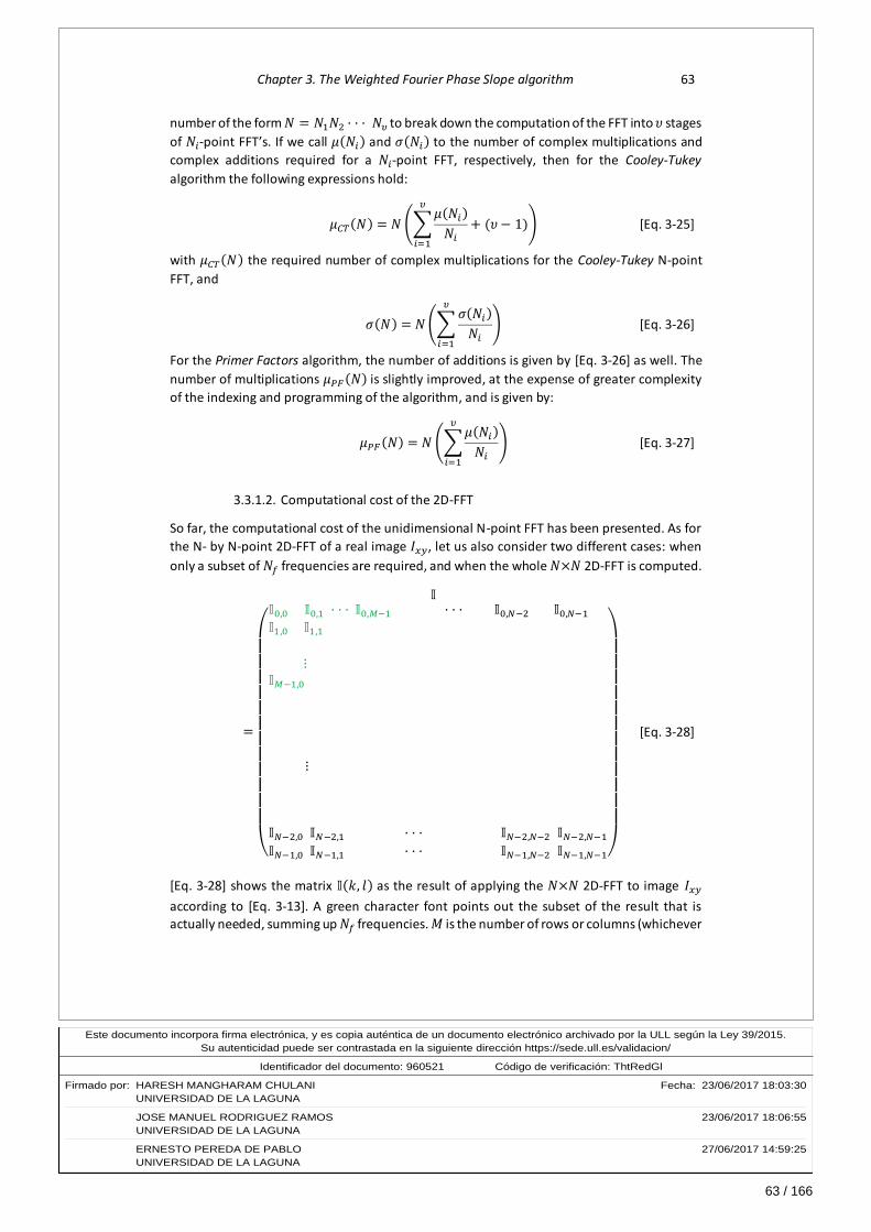
63 / 166
Este documento incorpora firma electrónica, y es copia auténtica de un documento electrónico archivado por la ULL según la Ley 39/2015.Su autenticidad puede ser contrastada en la siguiente dirección https://sede.ull.es/validacion/
Identificador del documento: 960521Código de verificación: ThtRedGl
Firmado por: HARESH MANGHARAM CHULANI Fecha: 23/06/2017 18:03:30UNIVERSIDAD DE LA LAGUNA
JOSE MANUEL RODRIGUEZ RAMOS 23/06/2017 18:06:55UNIVERSIDAD DE LA LAGUNA
ERNESTO PEREDA DE PABLO 27/06/2017 14:59:25UNIVERSIDAD DE LA LAGUNA
Chapter 3. The Weighted Fourier Phase Slope algorithm 63
number of the form 𝑁 = 𝑁1𝑁2 ··· 𝑁𝜐 to break down the computation of the FFT into 𝜐 stages
of 𝑁𝑖-point FFT’s. If we call 𝜇(𝑁𝑖) and 𝜎(𝑁𝑖) to the number of complex multiplications and
complex additions required for a 𝑁𝑖-point FFT, respectively, then for the Cooley-Tukey
algorithm the following expressions hold:
𝜇𝐶𝑇(𝑁) = 𝑁 (∑𝜇(𝑁𝑖)
𝑁𝑖
𝜐
𝑖=1
+ (𝜐 − 1)) [Eq. 3-25]
with 𝜇𝐶𝑇(𝑁) the required number of complex multiplications for the Cooley-Tukey N-point
FFT, and
𝜎(𝑁) = 𝑁(∑𝜎(𝑁𝑖)
𝑁𝑖
𝜐
𝑖=1
) [Eq. 3-26]
For the Primer Factors algorithm, the number of additions is given by [Eq. 3-26] as well. The
number of multiplications 𝜇𝑃𝐹(𝑁) is slightly improved, at the expense of greater complexity
of the indexing and programming of the algorithm, and is given by:
𝜇𝑃𝐹(𝑁) = 𝑁 (∑𝜇(𝑁𝑖)
𝑁𝑖
𝜐
𝑖=1
) [Eq. 3-27]
3.3.1.2. Computational cost of the 2D-FFT
So far, the computational cost of the unidimensional N-point FFT has been presented. As for
the N- by N-point 2D-FFT of a real image 𝐼𝑥𝑦, let us also consider two different cases: when
only a subset of 𝑁𝑓 frequencies are required, and when the whole 𝑁×𝑁 2D-FFT is computed.
𝕀
=
(
𝕀0,0𝕀0,1 ··· 𝕀0,𝑀−1 ··· 𝕀0,𝑁−2𝕀0,𝑁−1𝕀1,0𝕀1,1
⋮𝕀𝑀−1,0
⋮
𝕀𝑁−2,0𝕀𝑁−2,1 ··· 𝕀𝑁−2,𝑁−2𝕀𝑁−2,𝑁−1𝕀𝑁−1,0𝕀𝑁−1,1 ··· 𝕀𝑁−1,𝑁−2𝕀𝑁−1,𝑁−1)
[Eq. 3-28]
[Eq. 3-28] shows the matrix 𝕀(𝑘, 𝑙) as the result of applying the 𝑁×𝑁 2D-FFT to image 𝐼𝑥𝑦
according to [Eq. 3-13]. A green character font points out the subset of the result that is actually needed, summing up 𝑁𝑓 frequencies. 𝑀 is the number of rows or columns (whichever
64 / 166
Este documento incorpora firma electrónica, y es copia auténtica de un documento electrónico archivado por la ULL según la Ley 39/2015.Su autenticidad puede ser contrastada en la siguiente dirección https://sede.ull.es/validacion/
Identificador del documento: 960521Código de verificación: ThtRedGl
Firmado por: HARESH MANGHARAM CHULANI Fecha: 23/06/2017 18:03:30UNIVERSIDAD DE LA LAGUNA
JOSE MANUEL RODRIGUEZ RAMOS 23/06/2017 18:06:55UNIVERSIDAD DE LA LAGUNA
ERNESTO PEREDA DE PABLO 27/06/2017 14:59:25UNIVERSIDAD DE LA LAGUNA
64 Weighted Fourier Phase Slope
is less) spanned by the 𝑁𝑓 frequencies. In the example in [Eq. 3-28], the 2D-FFT can be
calculated in the following steps: first, N-point unidimensional FFT’s are applied to each of the
𝑁 rows of the real valued image 𝐼𝑥𝑦, and only the required 𝑀 frequencies are calculated (via
direct method), giving as a result a matrix of 𝑁 rows by 𝑀 columns; second, N-point
unidimensional FFT’s are applied to each of the resulting complex valued 𝑀 columns, and only
the frequencies pointed out by green font are calculated (via direct method), which in total sum up 𝑁𝑓 frequencies.
This process sums up a total of 𝑀𝑁2 complex by real multiplications and 𝑀𝑁(𝑁 − 1) complex additions for the 𝑁 horizontal N-point FFT’s; and 𝑁𝑓𝑁 complex multiplications and 𝑁𝑓(𝑁 −
1) complex additions for the 𝑀 vertical N-point FFT’s. Or, equivalently, 𝑁(2𝑀𝑁 + 4𝑁𝑓) real
multiplications and 𝑁(2𝑀𝑁 + 4𝑁𝑓) − (2𝑀𝑁 + 2𝑁𝑓) real additions.
When the complete 𝑁×𝑁 2D-FFT is required, then the unidimensional FFT’s are calculated
wholly through the most appropriate and efficient method, which depends upon the value of
𝑁, as it has been discussed above in point 3.3.1.1. The number of required operations is then
2𝑁 times the required number of operations for the N-point unidimensional FFT.
3.3.2. Computational cost of the WFPS algorithm
It will be proven in the next chapter that only a small number of spatial frequencies are
involved with significant weight in the computation of the WFPS centroiding method for
habitual system’s geometries and noises. These spatial frequencies are located at the
lowermost corner in the first quadrant of the Fourier domain, just as the green coloured
entries in the matrix of [Eq. 3-28]. In the derivation of the computational cost of the WFPS
algorithm, it will be assumed that the 2D-FFT’s involved are evaluated only at a small set of
spatial frequencies located in such manner.
On the other hand, two possible ways to compute the phase slopes in WFPS have been
presented in point 3.1, and here the computational cost for both of them will be derived. We
will start with the formulation for the phase slope in point 3.1.1. Table 3-1 summarizes the
computational cost of the WFPS algorithm for an N by N image 𝐼𝑥𝑦 for which 𝑁𝑓 Fourier phase
slopes are calculated following the expression [Eq. 3-17]. Only those operations directly
involving the live image 𝐼𝑥𝑦 are taken into account. The rest of operations can be computed
offline and their results stored, such as the product of coordinates and sines or cosines in [Eq.
3-17]. The total number of operations required is clearly dominated by the calculation of the
phase slopes: for each spatial frequency, ~6𝑁2 real multiplications are required, and the
same approximate number of real additions.
Table 3-2, on the other hand, summarizes the computational cost of the WFPS algorithm for
an N by N image 𝐼𝑥𝑦 when the 𝑁𝑓 Fourier phase slopes are calculated by direct evaluation of
the 2D-FFT’s in expression [Eq. 3-14]. The number of operations reflected for the 2D-FFT’s has
been derived in point 3.3.1.2, and M has the same meaning as in [Eq. 3-28]. Here, the total values are dominated by the computation of the 2D-FFT’s, and depend upon the number 𝑁𝑓
of spatial frequencies evaluated and their distribution in the frequency domain.

65 / 166
Este documento incorpora firma electrónica, y es copia auténtica de un documento electrónico archivado por la ULL según la Ley 39/2015.Su autenticidad puede ser contrastada en la siguiente dirección https://sede.ull.es/validacion/
Identificador del documento: 960521Código de verificación: ThtRedGl
Firmado por: HARESH MANGHARAM CHULANI Fecha: 23/06/2017 18:03:30UNIVERSIDAD DE LA LAGUNA
JOSE MANUEL RODRIGUEZ RAMOS 23/06/2017 18:06:55UNIVERSIDAD DE LA LAGUNA
ERNESTO PEREDA DE PABLO 27/06/2017 14:59:25UNIVERSIDAD DE LA LAGUNA
Chapter 3. The Weighted Fourier Phase Slope algorithm 65
#Real multiplications #Real additions #Real divisions 𝜶𝒙 𝑁2 𝑁2 − 1 𝜶𝒚 𝑁2 𝑁2 − 1 𝜷𝒙 𝑁2 𝑁2 − 1 𝜷𝒚 𝑁2 𝑁2 − 1 𝜸 𝑁2 𝑁2 − 1 𝜹 𝑁2 𝑁2 − 1
𝒅′𝒙 =𝜶𝒙𝜸 + 𝜷𝒙𝜹
𝜸𝟐 + 𝜹𝟐 4 2 1
𝒅′𝒚 =
𝜶𝒚𝜸 + 𝜷𝒚𝜹
𝜸𝟐 + 𝜹𝟐 2 1 1
Total per frequency 6𝑁2 + 6 6𝑁2 − 3 2
# frequencies ×𝑁𝑓
𝜮(𝒅′𝒙×𝑾𝒙) 𝑁𝑓 𝑁𝑓 − 1
𝜮(𝒅′𝒚×𝑾𝒚) 𝑁𝑓 𝑁𝑓 − 1
TOTAL (approx.) ~6𝑁𝑓𝑁2 ~6𝑁𝑓𝑁
2 2𝑁𝑓
Table 3-1. Computational cost of the WFPS algorithm for an N by N image 𝐼𝑥𝑦 following the computation of the
Fourier phase slopes according to equation [Eq. 3-17] and selecting 𝑁𝑓 spatial frequencies. Total values are
approximated assuming 𝑁2 ≫ 1.
#Real multiplications
#Real additions #Real divisions
𝟐𝑫_𝑭𝑭𝑻{𝒙𝑰𝒙𝒚} 𝑁(2𝑀𝑁 + 4𝑁𝑓) 𝑁(2𝑀𝑁 + 4𝑁𝑓) −
(2𝑀𝑁 + 2𝑁𝑓)
𝟐𝑫_𝑭𝑭𝑻{𝒚𝑰𝒙𝒚} 𝑁(2𝑀𝑁 + 4𝑁𝑓) 𝑁(2𝑀𝑁 + 4𝑁𝑓) −
(2𝑀𝑁 + 2𝑁𝑓)
𝟐𝑫_𝑭𝑭𝑻{𝑰𝒙𝒚} 𝑁(2𝑀𝑁 + 4𝑁𝑓) 𝑁(2𝑀𝑁 + 4𝑁𝑓) −
(2𝑀𝑁 + 2𝑁𝑓)
Total 2D-FFT’s (direct method)
3𝑁(2𝑀𝑁 + 4𝑁𝑓) 3[𝑁(2𝑀𝑁 + 4𝑁𝑓) −
(2𝑀𝑁 + 2𝑁𝑓)]
𝒅′𝒙 =𝜶𝒙𝜸 + 𝜷𝒙𝜹
𝜸𝟐 + 𝜹𝟐 4 2 1
𝒅′𝒚 =
𝜶𝒚𝜸 + 𝜷𝒚𝜹
𝜸𝟐 + 𝜹𝟐 2 1 1
Total per frequency 6 3 2
# frequencies ×𝑁𝑓
𝜮(𝒅′𝒙×𝑾𝒙) 𝑁𝑓 𝑁𝑓 − 1
𝜮(𝒅′𝒚×𝑾𝒚) 𝑁𝑓 𝑁𝑓 − 1
TOTAL (approx.) ~6𝑀𝑁2+ 12𝑁𝑓𝑁 ~6𝑀𝑁(𝑁 − 1)+ 12𝑁𝑓𝑁
2𝑁𝑓
Table 3-2. Computational cost of the WFPS algorithm for an N by N image 𝐼𝑥𝑦 following the computation of the
Fourier phase slopes according to equation [Eq. 3-14] by direct method computation of the 2D-FFT’s focusing on 𝑁𝑓 spatial frequencies exclusively. M has the same meaning as in [Eq. 3-28]. Total values are approximated
assuming 𝑁2 ≫ 1.

66 / 166
Este documento incorpora firma electrónica, y es copia auténtica de un documento electrónico archivado por la ULL según la Ley 39/2015.Su autenticidad puede ser contrastada en la siguiente dirección https://sede.ull.es/validacion/
Identificador del documento: 960521Código de verificación: ThtRedGl
Firmado por: HARESH MANGHARAM CHULANI Fecha: 23/06/2017 18:03:30UNIVERSIDAD DE LA LAGUNA
JOSE MANUEL RODRIGUEZ RAMOS 23/06/2017 18:06:55UNIVERSIDAD DE LA LAGUNA
ERNESTO PEREDA DE PABLO 27/06/2017 14:59:25UNIVERSIDAD DE LA LAGUNA
66 Weighted Fourier Phase Slope
Let us take as an example, for the purpose of comparing both methods of computing the
phase slopes, a case where 𝑁 = 12, 𝑁𝑓 = 6 and 𝑀 = 3. Following the computation in [Eq. 3-
17] and according to Table 3-1, the required number of operations would be ~5184 real
multiplications per image and the same approximate number of real sums. Whereas following
the 2D-FFT’s computation in [Eq. 3-14] and according to Table 3-2, the required number of
operations would be ~3456 real multiplications and ~3240 real sums per image, slightly less
than in the previous case, but in the same order of magnitude.
3.3.3. Computational cost of the TCoG and WCoG algorithms
Table 3-3 and Table 3-4 summarize the computational cost of the TCoG and the WCoG algorithms, respectively, for an N by N image 𝐼𝑥𝑦, following the computation described in
equations [Eq. 1-26] to [Eq. 1-28]. Threshold T is predetermined and an input to the TCoG
algorithm. Similarly, weights W are predetermined, fixed, and an input to the WCoG
algorithm. The total number of operations is an order of magnitude less than in the WFPS
algorithm case, approximately.
#Real multiplications
#Real additions
#Real divisions
#Real comparisons
𝑰𝒙𝒚 − 𝑻 𝑁2 𝑁2 𝜮𝒙(𝑰𝒙𝒚 − 𝑻) 𝑁2 𝑁2 − 1
𝜮𝒚(𝑰𝒙𝒚 − 𝑻) 𝑁2 𝑁2 − 1 𝜮(𝑰𝒙𝒚 − 𝑻) 𝑁2 − 1
𝜮𝒙(𝑰𝒙𝒚 − 𝑻)𝜮(𝑰𝒙𝒚 − 𝑻)⁄
1
𝜮𝒚(𝑰𝒙𝒚 − 𝑻)𝜮(𝑰𝒙𝒚 − 𝑻)⁄
1
TOTAL 2𝑁2 4𝑁2 − 3 2 𝑁2
Table 3-3. Computational cost of the TCoG algorithm for an N by N image 𝐼𝑥𝑦 following the computation
described in [Eq. 1-27]. Threshold T is an input to the algorithm.
#Real multiplications #Real additions #Real divisions 𝑾𝒙𝒚𝑰𝒙𝒚 𝑁2 𝜮𝒙𝑾𝒙𝒚𝑰𝒙𝒚 𝑁2 𝑁2 − 1 𝜮𝒚𝑾𝒙𝒚𝑰𝒙𝒚 𝑁2 𝑁2 − 1 𝜮𝑾𝒙𝒚𝑰𝒙𝒚 𝑁2 − 1 𝜮𝒙𝑾𝒙𝒚𝑰𝒙𝒚
𝜮𝑾𝒙𝒚𝑰𝒙𝒚⁄
1
𝜮𝒚𝑾𝒙𝒚𝑰𝒙𝒚𝜮𝑾𝒙𝒚𝑰𝒙𝒚⁄
1
TOTAL 3𝑁2 3𝑁2 − 3 2
Table 3-4. Computational cost of the WCoG algorithm for an N by N image 𝐼𝑥𝑦 following the computation
described in [Eq. 1-26] and [Eq. 1-28]. Weights 𝑊𝑥𝑦 are predetermined and an input to the algorithm.

67 / 166
Este documento incorpora firma electrónica, y es copia auténtica de un documento electrónico archivado por la ULL según la Ley 39/2015.Su autenticidad puede ser contrastada en la siguiente dirección https://sede.ull.es/validacion/
Identificador del documento: 960521Código de verificación: ThtRedGl
Firmado por: HARESH MANGHARAM CHULANI Fecha: 23/06/2017 18:03:30UNIVERSIDAD DE LA LAGUNA
JOSE MANUEL RODRIGUEZ RAMOS 23/06/2017 18:06:55UNIVERSIDAD DE LA LAGUNA
ERNESTO PEREDA DE PABLO 27/06/2017 14:59:25UNIVERSIDAD DE LA LAGUNA
Chapter 3. The Weighted Fourier Phase Slope algorithm 67
3.3.4. Computational cost of the Cross Correlation algorithm
For the evaluation of the computational cost of the CC algorithm, cross-correlation in the
Fourier domain is assumed, and subsequent application of the TCoG algorithm to the
correlation figure in order to obtain the final centroid coordinates. Thus, the CC algorithm,
applied to an N by N pixels size live image 𝐼𝑥𝑦 and a Nref by Nref pixels size reference image
𝐼𝑟𝑒𝑓, is composed of the following operations:
1. Zero padding the N by N pixels size live image 𝐼𝑥𝑦 to complete a Nfft by Nfft pixels size
image, being Nfft ≥ N + Nref -1. This is necessary to avoid aliasing in the image domain,
since the signal in the Fourier domain is discretized.
2. Calculating the Nfft by Nfft 2D-FFT of the zero-padded live image.
3. Multiplying in the Fourier domain live and reference images: 𝕀×𝕀𝑟𝑒𝑓 . The reference
image in the Fourier domain has been precalculated with the adequate resolution.
Matrices are multiplied element-wise.
4. Assuming no interpolation or increase in the original image resolution is required, a
Nfft by Nfft inverse 2D-FFT gives the correlation figure.
5. A TCoG algorithm is applied to the correlation figure and the final centroid obtained.
#Real
multiplications #Real additions
#Real divisions
#Real comparisons
𝟐𝑫_𝑭𝑭𝑻{𝑰𝒙𝒚} 8𝑁𝑓𝑓𝑡𝜇(𝑁𝑓𝑓𝑡) 4𝑁𝑓𝑓𝑡 (𝜇(𝑁𝑓𝑓𝑡) + 𝜎(𝑁𝑓𝑓𝑡))
𝕀×𝕀𝒓𝒆𝒇 4𝑁𝑓𝑓𝑡2 2𝑁𝑓𝑓𝑡
2
𝒊_𝟐𝑫_𝑭𝑭𝑻{𝕀×
𝕀𝒓𝒆𝒇} 8𝑁𝑓𝑓𝑡𝜇(𝑁𝑓𝑓𝑡) 4𝑁𝑓𝑓𝑡 (𝜇(𝑁𝑓𝑓𝑡) + 𝜎(𝑁𝑓𝑓𝑡))
TCoG 2𝑁𝑓𝑓𝑡2 4𝑁𝑓𝑓𝑡
2 − 3 2 𝑁𝑓𝑓𝑡2
TOTAL
(approx.)
𝑁𝑓𝑓𝑡(16𝜇(𝑁𝑓𝑓𝑡) +
6𝑁𝑓𝑓𝑡)
~𝑁𝑓𝑓𝑡(8𝜇(𝑁𝑓𝑓𝑡) +
8𝜎(𝑁𝑓𝑓𝑡) + 6𝑁𝑓𝑓𝑡) 2 𝑁𝑓𝑓𝑡
2
Table 3-5. Computational cost of the CC algorithm for an N by N image 𝐼𝑥𝑦 and an Nref by Nref image 𝐼𝑟𝑒𝑓. CC
computation is done in the Fourier domain, with an Nfft by Nfft bi-dimensional FFT, being Nfft ≥ N + Nref -1. TCoG is applied to the correlation figure, without previous interpolation.
Table 3-5 summarizes the computational cost of the above described CC algorithm. Notation
in equations [Eq. 3-25] to [Eq. 3-27] has been followed: 𝜇(𝑁𝑓𝑓𝑡) is the number of complex
multiplications for an 𝑁𝑓𝑓𝑡-point unidimensional FFT, and 𝜎(𝑁𝑓𝑓𝑡) is the number of complex
additions. Whole 𝑁𝑓𝑓𝑡×𝑁𝑓𝑓𝑡 bi-dimensional FFT’s are calculated, and so, the number of
operations for a 2D-FFT is 2𝑁𝑓𝑓𝑡 times that required for a unidimensional FFT. Inverse 2D-FFT
requires the same number of operations as the direct 2D-FFT.
The total number of multiplications and additions for the CC algorithm depends upon the
chosen size of the 2D-FFT, which is in any case bigger than the live image’s size. Also, the
efficiency of the unidimensional FFT’s calculation plays an important role through the values
of 𝜇(𝑁𝑓𝑓𝑡) and 𝜎(𝑁𝑓𝑓𝑡), and this depends upon the chosen value of 𝑁𝑓𝑓𝑡. Comparison with
WFPS algorithm will be made through examples in the following point.
68 / 166
Este documento incorpora firma electrónica, y es copia auténtica de un documento electrónico archivado por la ULL según la Ley 39/2015.Su autenticidad puede ser contrastada en la siguiente dirección https://sede.ull.es/validacion/
Identificador del documento: 960521Código de verificación: ThtRedGl
Firmado por: HARESH MANGHARAM CHULANI Fecha: 23/06/2017 18:03:30UNIVERSIDAD DE LA LAGUNA
JOSE MANUEL RODRIGUEZ RAMOS 23/06/2017 18:06:55UNIVERSIDAD DE LA LAGUNA
ERNESTO PEREDA DE PABLO 27/06/2017 14:59:25UNIVERSIDAD DE LA LAGUNA
68 Weighted Fourier Phase Slope
3.3.5. Comparison between algorithms through examples and conclusions
As an example of SHWFS configuration, for the purpose of comparing the computational cost
of the centroiding algorithms seen in the previous points, we will take the case of an ELT with
80 by 80 subpupils and 12 by 12 pixels of the detector assigned to each subpupil. We will
assign for the computation of all the centroids of a SHWFS image an allowed latency of 100
µsecs, and then work out the computational power required for the computation of each
centroiding method for the whole pupil or SHWFS image.
For the WFPS algorithm, we again assume that the number of spatial frequencies involved in
the computation of Fourier phase slopes is 𝑁𝑓 = 6, and the columns and rows spanned by
them is 𝑀 = 3. We also assume that the 2D-FFT’s are of size 12 by 12, same as the subpupil
image’s size. Following [Eq. 3-17] for the computation of the phase slopes and according to
Table 3-1, the required number of operations would be ~5184 real multiplications per image
and the same approximate number of real sums, per subpupil and per frame. Regarding both
multiplications and additions as floating point operations, this makes a computational
requirement of ~665 Gflops. Whereas partially calculating the 2D-FFT’s in [Eq. 3-14] and
according to Table 3-2, the required number of operations would be ~3456 real
multiplications and ~3240 real sums per image and per subpupil, which gives a
computational requirement of ~430 Gflops.
For the TCoG algorithm, the number of required operations according to Table 3-3 is ~1008
floating point operations per image per subpupil, including real comparisons. Whereas for the
WCoG algorithm, the number of required operations according to Table 3-4 is ~864 floating
point operations per image per subpupil. This implies a total computational requirement of
~65 Gflops for the TCoG and ~55 Gflops for the WCoG.
As for the CC algorithm, there are several options to be considered. First, the size of the
reference image is an option. We will consider a favourable case with Nref = 4 pixels, and a less
favourable case with Nref = 6 pixels. Second, the size of the unidimensional FFT (Nfft) affects
computational efficiency.
In the case of Nref = 4 pixels, the most efficient value for Nfft is 16. The efficient schemes for a
power of 2 size unidimensional FFT can be applied, resulting in µ(16)=32 complex
multiplications and σ(16)=64 complex additions. Following the derivation summarized in
Table 3-5, this makes a requirement of ~9728 real multiplications, ~13824 real additions
and 256 real comparisons per subpupil per frame, for a total of ~1524 Gflops.
With Nref = 6 pixels the situation is less favourable. By choosing Nfft=18, we have µ(18)=
σ(16)=144 complex multiplications or additions, and a total requirement of ~5578 Gflops.
Choosing Nfft=32 makes the unidimensional FFT’s more efficient, with µ(32)=80 complex
multiplications and σ(32)=160 complex additions, but the 2D-FFT size becomes much larger
and the total computational requirement is ~7406 Gflops.
Table 3-6 summarizes the results just obtained in this example.
In the first example described above, 80 x 80 subpupils in an ELT implies a subpupil diameter
or side size of around half a metre, for a pupil size of ~40 metres. On the other hand, Fried

69 / 166
Este documento incorpora firma electrónica, y es copia auténtica de un documento electrónico archivado por la ULL según la Ley 39/2015.Su autenticidad puede ser contrastada en la siguiente dirección https://sede.ull.es/validacion/
Identificador del documento: 960521Código de verificación: ThtRedGl
Firmado por: HARESH MANGHARAM CHULANI Fecha: 23/06/2017 18:03:30UNIVERSIDAD DE LA LAGUNA
JOSE MANUEL RODRIGUEZ RAMOS 23/06/2017 18:06:55UNIVERSIDAD DE LA LAGUNA
ERNESTO PEREDA DE PABLO 27/06/2017 14:59:25UNIVERSIDAD DE LA LAGUNA
Chapter 3. The Weighted Fourier Phase Slope algorithm 69
parameters in the visible wavelength for a good observing site are in the order of 15-20 cm.
Thus, subpupil size to Fried parameter ratios in this example are in the order of 3. In open
loop observations, a bigger than 12 x 12 pixels FoV is required to cope with the spots’ tilt
movements. So here we illustrate a second example where, in an ELT with 80 x 80 subpupils,
this time 16 x 16 pixels at the detector are assigned to each subpupil. Table 3-7 summarizes
the results obtained in this second example.
COMPUTATIONAL COST COMPARISON
80 x 80 subpupils, 16 x 16 pixels per subpupil, 100 µsecs. latency WCoG TCoG
~98 Gflops ~115 Gflops WFPS CC
Nf = 6 frequencies, spanning M = 3 columns
Nref = 4, Nfft = 20
Phase slopes as f(α,β,γ,δ) [Eq. 3-17] ~7706 Gflops ~1180 Gflops Nref = 6, Nfft = 24 Partial computation of 2D-FFT’s (Nfft=16) ~11096 Gflops ~719 Gflops Nref = 6, Nfft = 32 ~7406 Gflops Table 3-7. Example of computational cost comparison between WCoG, TCoG, WFPS and CC algorithms, for an
ELT with 80 x 80 subpupils, 16 x 16 pixels per subpupil at the detector and 100 µsecs budgeted latency for centroids computation.
COMPUTATIONAL COST COMPARISON
80 x 80 subpupils, 12 x 12 pixels per subpupil, 100 µsecs. latency WCoG TCoG
~55 Gflops ~65 Gflops WFPS CC
Nf = 6 frequencies, spanning M = 3 columns
Nref = 4, Nfft = 16
Phase slopes as f(α,β,γ,δ) [Eq. 3-17] ~1524 Gflops ~665 Gflops Nref = 6, Nfft = 18
Partial computation of 2D-FFT’s (Nfft=12) ~5578 Gflops ~430 Gflops Nref = 6, Nfft = 32 ~7406 Gflops Table 3-6. Example of computational cost comparison between WCoG, TCoG, WFPS and CC algorithms, for an
ELT with 80 x 80 subpupils, 12 x 12 pixels per subpupil at the detector and 100 µsecs budgeted latency for centroids computation.

70 / 166
Este documento incorpora firma electrónica, y es copia auténtica de un documento electrónico archivado por la ULL según la Ley 39/2015.Su autenticidad puede ser contrastada en la siguiente dirección https://sede.ull.es/validacion/
Identificador del documento: 960521Código de verificación: ThtRedGl
Firmado por: HARESH MANGHARAM CHULANI Fecha: 23/06/2017 18:03:30UNIVERSIDAD DE LA LAGUNA
JOSE MANUEL RODRIGUEZ RAMOS 23/06/2017 18:06:55UNIVERSIDAD DE LA LAGUNA
ERNESTO PEREDA DE PABLO 27/06/2017 14:59:25UNIVERSIDAD DE LA LAGUNA
70 Weighted Fourier Phase Slope
We are considering in Table 3-7 the generic formulation of the Prime Factors FFT algorithm
([Eq. 3-26] and [Eq. 3-27]), and so µ(20) = σ(20)=180 and µ(24) = σ(24)=216. In this second
example, the most efficient value for the CC algorithm is Nfft = 32.
Both examples are showing us an increase in computational cost of one order of magnitude
when shifting from CoG derived algorithms to WFPS algorithm, and again an increase of
another order of magnitude when comparing WFPS with the CC algorithm, except when the
case is very favourable to the CC algorithm, such as when the sum of N and Nref is a power of
2. Even in this latter case, the CC algorithm requires more than 3 times the computational
power required for the WFPS algorithm.
Finally, let us compare the required computational power obtained in these examples for the
evaluated centroiding algorithms with commercial elements of computation. Let us take, as
an example, systems based on the Tesla G80 GPU from Nvidia5. The CoG based centroiding
algorithms can fit into a C870 PCI Express computing module, comprising one G80 based GPU,
and hence 128 streaming processor cores at 1.35 GHz, for a total processing power of 345.6
GFlops, computed in a conservative manner. The WFPS algorithm would require one S870
computing server which comes in a 1U form factor for a standard 19-inch rack and comprises
four G80 based GPU’s, making up a total processing power of 1382.4 Gflops. Cross correlation,
for the 16 x 16 FoV case, would require at least half a dozen of S870 servers.
5 The processing power specifications of these elements have been taken from the English version of Wikipedia, at the “Nvidia Tesla” entry, as of May, 2017.

71 / 166
Este documento incorpora firma electrónica, y es copia auténtica de un documento electrónico archivado por la ULL según la Ley 39/2015.Su autenticidad puede ser contrastada en la siguiente dirección https://sede.ull.es/validacion/
Identificador del documento: 960521Código de verificación: ThtRedGl
Firmado por: HARESH MANGHARAM CHULANI Fecha: 23/06/2017 18:03:30UNIVERSIDAD DE LA LAGUNA
JOSE MANUEL RODRIGUEZ RAMOS 23/06/2017 18:06:55UNIVERSIDAD DE LA LAGUNA
ERNESTO PEREDA DE PABLO 27/06/2017 14:59:25UNIVERSIDAD DE LA LAGUNA
Chapter 4. Numerical simulations at subpupil level
In this chapter, the behaviour of the Weighted Fourier Phase Slope algorithm and its
comparison with other known centroiding methods will be evaluated and understood
through numerical simulations at a subpupil level. In this kind of simulation, a single Shack-
Hartmann subaperture is illuminated with a wavefront fulfilling Kolmogorov phase statistiscs;
an image is thus formed at the detector situated at the microlense’s focal plane, and the
appropriate detector’s gain and noise model is applied to obtain a close to real subpupil
image. The incident phase tilt is then estimated by applying different centroiding methods to
this image, and the result is compared to the known applied tilt, thus obtaining an estimation
error for each centroiding method that allows for their behaviour comparison. Light level flux,
detector noises, FoV, atmospheric turbulence strength and any other parameter defining the
system can be easily changed in simulation, and hence sensitivity and linearity of the
centroiding methods with different FoV’s, and their robustness against such effects as higher
orders of turbulence phase, can be easily evaluated. Moreover, optimization of every
centroiding method’s parameters, such as MAP weights for the WFPS as expressed in [Eq. 3-
22], is achieved through this type of simulation.
4.1. The simulation method
4.1.1. Simulation of Kolmogorov phase frames
The approach to simulate independent Kolmogorov phase frames has been taken from
Roddier, 1990. Roddier’s approach consists in expanding the phase into a functions base for
which the coefficients covariance matrix is known and diagonal, that is, the contribution of
each function to the total phase energy is known and uncorrelated to the other functions’
contributions. Such a base is called a Karhunen-Loève base of functions.
A Kolmogorov phase 𝜙 is characterized by its spatial structure function as expressed in [Eq.
1-5]:

72 / 166
Este documento incorpora firma electrónica, y es copia auténtica de un documento electrónico archivado por la ULL según la Ley 39/2015.Su autenticidad puede ser contrastada en la siguiente dirección https://sede.ull.es/validacion/
Identificador del documento: 960521Código de verificación: ThtRedGl
Firmado por: HARESH MANGHARAM CHULANI Fecha: 23/06/2017 18:03:30UNIVERSIDAD DE LA LAGUNA
JOSE MANUEL RODRIGUEZ RAMOS 23/06/2017 18:06:55UNIVERSIDAD DE LA LAGUNA
ERNESTO PEREDA DE PABLO 27/06/2017 14:59:25UNIVERSIDAD DE LA LAGUNA
72 Weighted Fourier Phase Slope
𝐷𝜙(𝑟) = 6.88 (𝑟
𝑟0)5/3
[Eq. 4-1]
with 𝑟 being the distance between the two evaluated points in space and 𝑟0 being the Fried
parameter which characterizes the turbulence strength. Such a structure function gives place
to a Wiener spatial power spectrum expressed as:
𝑊𝜙(𝑓) = 0.023
𝑟05/3𝑓11/3
[Eq. 4-2]
where 𝑓 is the wave spatial frequency. For a Kolmogorov phase expressed into a Zernike
functions expansion, such as in [Eq. 1-21]:
𝜙(𝑟, 𝜃) = 𝜙(𝑅𝜌, 𝜃) = ∑𝑐𝑗𝑍𝑗(𝜌, 𝜃)
𝑗
[Eq. 4-3]
with 𝑟 and 𝜃 the polar radial and azimuthal coordinates, respectively, and 𝜌 the radial
coordinate normalized by the aperture radius 𝑅, knowledge of the Wiener power spectrum
function in [Eq. 4-2] allows to obtain the covariance matrix of the Zernike coefficients 𝑐𝑗 (Noll,
1976; Roddier, 1990). The result thus obtained is expressed as:
⟨𝑐𝑗∗𝑐𝑗′⟩ =
𝐾𝑧𝑧′𝛿𝑧Γ [(𝑛 + 𝑛′ −53) /2]
(𝐷/𝑟0)5/3
Γ [(𝑛 − 𝑛′ +173 ) /2] Γ [(𝑛′ − 𝑛 +
173 ) /2]Γ [(𝑛 + 𝑛
′ +233 ) /2]
[Eq. 4-4]
𝛿𝑧 is a logical Kronecker symbol the value of which is:
𝛿𝑧 = (𝑚 = 𝑚′) ∧ (𝑝𝑎𝑟𝑖𝑡𝑦(𝑗, 𝑗′)̅̅ ̅̅ ̅̅ ̅̅ ̅̅ ̅̅ ̅̅ ̅̅ ∨ (𝑚 = 0)) [Eq. 4-5]
and 𝑛, 𝑚, 𝑛′ and 𝑚′ are the radial and azimuthal orders of 𝑍𝑗 and 𝑍𝑗′. In other words,
covariance can only be non-zero for Zernike functions with the same azimuthal order.
Furthermore, for Zernike functions with non-zero azimuthal order, the parity of their indexes
must be the same, i.e., the covariance between an even and an odd function is zero.
As for the 𝐾𝑧𝑧′ factor, its value is:
𝐾𝑧𝑧′ = 2.2698(−1)(𝑛+𝑛′−2𝑚)/2√(𝑛 + 1)(𝑛′ + 1) [Eq. 4-6]
Finally, 𝐷/𝑟0 is the ratio of the pupil’s diameter to the Fried parameter.
This covariance of Zernike’s coefficients for Kolmogorov turbulence as expressed in [Eq. 4-4]
was found already implemented in an IDL subroutine for the CAOS simulation tool6, adapted
6 CAOS stands for Code for Adaptive Optics Systems, and is a programming environment for AO modelling and post-AO imaging, based on IDL language. IDL stands for Interactive Data Language, and is a programming language used for data analysis.

73 / 166
Este documento incorpora firma electrónica, y es copia auténtica de un documento electrónico archivado por la ULL según la Ley 39/2015.Su autenticidad puede ser contrastada en la siguiente dirección https://sede.ull.es/validacion/
Identificador del documento: 960521Código de verificación: ThtRedGl
Firmado por: HARESH MANGHARAM CHULANI Fecha: 23/06/2017 18:03:30UNIVERSIDAD DE LA LAGUNA
JOSE MANUEL RODRIGUEZ RAMOS 23/06/2017 18:06:55UNIVERSIDAD DE LA LAGUNA
ERNESTO PEREDA DE PABLO 27/06/2017 14:59:25UNIVERSIDAD DE LA LAGUNA
Chapter 4. Numerical simulations at subpupil level 73
to work in the MATLAB™ environment and used to generate the phase frames for all the
simulations described in this chapter.
0.4557 0 0 0 0 0 -0.0144 0 0 0 0 0 0 0 0 0.4557 0 0 0 -0.0144 0 0 0 0 0 0 0 0 0 0 0.0236 0 0 0 0 0 0 -0.0039 0 0 0 0 0 0 0 0.0236 0 0 0 0 0 0 0 -0.0039 0 0 0 0 0 0 0.0236 0 0 0 0 0 -0.0039 0 0 0 0 -0.0144 0 0 0 0.0063 0 0 0 0 0 0 0 0
-0.0144 0 0 0 0 0 0.0063 0 0 0 0 0 0 0 0 0 0 0 0 0 0 0.0063 0 0 0 0 0 0 0 0 0 0 0 0 0 0 0.0063 0 0 0 0 0 0 0 -0.0039 0 0 0 0 0 0 0.0025 0 00 0 0 0 0 0 0 -0.0039 0 0 0 0 0 0.0025 00 0 0 0 0 0 -0.0039 0 0 0 0 0 0 0 0.0025 0 0 0 0 0 0 0 0 0 0 0 0 0 0 0.0025 0
0 0 0 0 0 0 0 0 0 0 0 0 0 0.0025
Table 4-1. Covariance matrix for the first 14 zero mean Zernike functions (Z2 to Z15) of Kolmogorov turbulence phase. (D/r0)5/3 units.
Table 4-1 shows the covariance matrix 𝑉𝑍 for the first 15 Zernike functions except 𝑍1 or piston,
for a Kolmogorov turbulence phase, in (𝐷/𝑟0)5/3 units. Off diagonal non-zero elements
correspond to the cross covariance of terms with same azimuthal order and same parity,
according to [Eq. 4-5]. Thus, Kolmogorov phase cannot be simulated by generating random
independent Zernike coefficients, because these non-zero cross covariances should be taken
into account.
The Zernike expansion of the phase as in [Eq. 4-3] can be vectorised and expressed as in [Eq.
1-22]:
𝜙 = 𝑍𝑐 [Eq. 4-7]
with 𝜙 a column vector of phases at the coordinates of interest, 𝑍 a matrix with as many
columns as Zernike functions and as many rows as coordinates in which the functions are
evaluated, and 𝑐 a column vector of Zernike coefficients. The covariance matrix 𝑉𝑍 can then
be expressed as:
𝑉𝑍 = ⟨𝑐𝑐𝑇⟩ [Eq. 4-8]
𝑐 is regarded as real-valued, and 𝑐𝑇 is the transpose of 𝑐. Angular brackets denote temporal
averaging. Being 𝑉𝑍 a Hermitian matrix, a unitary matrix 𝑈 and a diagonal matrix 𝑉𝐾𝐿 can be
found such that:
𝑉𝐾𝐿 = 𝑈𝑉𝑍𝑈𝑇 [Eq. 4-9]
by a singular value decomposition (SVD) of 𝑉𝑍, for example. If we employ the unitary matrix
𝑈 for a function set transformation, the new coefficient vector would be:

74 / 166
Este documento incorpora firma electrónica, y es copia auténtica de un documento electrónico archivado por la ULL según la Ley 39/2015.Su autenticidad puede ser contrastada en la siguiente dirección https://sede.ull.es/validacion/
Identificador del documento: 960521Código de verificación: ThtRedGl
Firmado por: HARESH MANGHARAM CHULANI Fecha: 23/06/2017 18:03:30UNIVERSIDAD DE LA LAGUNA
JOSE MANUEL RODRIGUEZ RAMOS 23/06/2017 18:06:55UNIVERSIDAD DE LA LAGUNA
ERNESTO PEREDA DE PABLO 27/06/2017 14:59:25UNIVERSIDAD DE LA LAGUNA
74 Weighted Fourier Phase Slope
𝑑 = 𝑈c [Eq. 4-10]
for which the covariance matrix is:
⟨𝑑𝑑𝑇⟩ = ⟨𝑈𝑐𝑐𝑇𝑈𝑇⟩ = 𝑈⟨𝑐𝑐𝑇⟩𝑈𝑇 = 𝑈𝑉𝑍𝑈𝑇 = 𝑉𝐾𝐿 [Eq. 4-11]
which is diagonal, and the phase in [Eq. 4-7] can be expressed as
𝜙 = (𝑍𝑈𝑇)𝑑 = 𝐾_𝐿𝑑 [Eq. 4-12]
This means that, by developing the Kolmogorov phase 𝜙 into a linear combination of a set of
functions defined by 𝐾_𝐿 = 𝑍𝑈𝑇, the resultant coefficients 𝑑 have a diagonal covariance
matrix 𝑉𝐾𝐿 and, hence, are statistically independent. Such a function base is called a
Karhunen-Loève base. The method for simulating Kolmogorov phase frames has therefore
consisted of generating random 𝑑 coefficients with Gaussian distribution, zero mean and
variance determined by 𝑉𝐾𝐿, and applying them to a phase expansion into a Karhunen-Loève
base of functions according to [Eq. 4-12].
4.1.1.1. Verification of the phase simulation method
Figure 4-1. Comparison of theoretical Kolmogorov phase structure ([Eq. 4-1], solid line) with the phase structure obtained from a series of 50000 simulated phase frames, with D/r0=1 and 32x32 pixels resolution per frame
(diamond shapes).
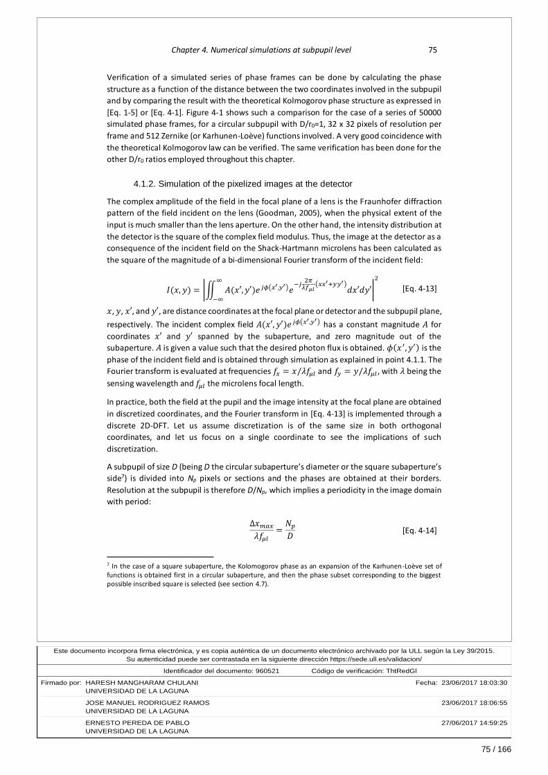
75 / 166
Este documento incorpora firma electrónica, y es copia auténtica de un documento electrónico archivado por la ULL según la Ley 39/2015.Su autenticidad puede ser contrastada en la siguiente dirección https://sede.ull.es/validacion/
Identificador del documento: 960521Código de verificación: ThtRedGl
Firmado por: HARESH MANGHARAM CHULANI Fecha: 23/06/2017 18:03:30UNIVERSIDAD DE LA LAGUNA
JOSE MANUEL RODRIGUEZ RAMOS 23/06/2017 18:06:55UNIVERSIDAD DE LA LAGUNA
ERNESTO PEREDA DE PABLO 27/06/2017 14:59:25UNIVERSIDAD DE LA LAGUNA
Chapter 4. Numerical simulations at subpupil level 75
Verification of a simulated series of phase frames can be done by calculating the phase
structure as a function of the distance between the two coordinates involved in the subpupil
and by comparing the result with the theoretical Kolmogorov phase structure as expressed in
[Eq. 1-5] or [Eq. 4-1]. Figure 4-1 shows such a comparison for the case of a series of 50000
simulated phase frames, for a circular subpupil with D/r0=1, 32 x 32 pixels of resolution per
frame and 512 Zernike (or Karhunen-Loève) functions involved. A very good coincidence with
the theoretical Kolmogorov law can be verified. The same verification has been done for the
other D/r0 ratios employed throughout this chapter.
4.1.2. Simulation of the pixelized images at the detector
The complex amplitude of the field in the focal plane of a lens is the Fraunhofer diffraction
pattern of the field incident on the lens (Goodman, 2005), when the physical extent of the
input is much smaller than the lens aperture. On the other hand, the intensity distribution at
the detector is the square of the complex field modulus. Thus, the image at the detector as a
consequence of the incident field on the Shack-Hartmann microlens has been calculated as
the square of the magnitude of a bi-dimensional Fourier transform of the incident field:
𝐼(𝑥, 𝑦) = |∬ 𝐴(𝑥′, 𝑦′)𝑒𝑗𝜙(𝑥′,𝑦′)𝑒
−𝑗2𝜋𝜆𝑓𝜇𝑙
(𝑥𝑥′+𝑦𝑦′)𝑑𝑥′𝑑𝑦′
∞
−∞
|
2
[Eq. 4-13]
𝑥, 𝑦, 𝑥′, and 𝑦′, are distance coordinates at the focal plane or detector and the subpupil plane,
respectively. The incident complex field 𝐴(𝑥′, 𝑦′)𝑒𝑗𝜙(𝑥′,𝑦′) has a constant magnitude 𝐴 for
coordinates 𝑥′ and 𝑦′ spanned by the subaperture, and zero magnitude out of the
subaperture. 𝐴 is given a value such that the desired photon flux is obtained. 𝜙(𝑥 ′, 𝑦′) is the
phase of the incident field and is obtained through simulation as explained in point 4.1.1. The
Fourier transform is evaluated at frequencies 𝑓𝑥 = 𝑥/𝜆𝑓𝜇𝑙 and 𝑓𝑦 = 𝑦/𝜆𝑓𝜇𝑙 , with 𝜆 being the
sensing wavelength and 𝑓𝜇𝑙 the microlens focal length.
In practice, both the field at the pupil and the image intensity at the focal plane are obtained
in discretized coordinates, and the Fourier transform in [Eq. 4-13] is implemented through a
discrete 2D-DFT. Let us assume discretization is of the same size in both orthogonal
coordinates, and let us focus on a single coordinate to see the implications of such
discretization.
A subpupil of size D (being D the circular subaperture’s diameter or the square subaperture’s
side7) is divided into Np pixels or sections and the phases are obtained at their borders.
Resolution at the subpupil is therefore D/Np, which implies a periodicity in the image domain
with period:
Δ𝑥𝑚𝑎𝑥𝜆𝑓𝜇𝑙
=𝑁𝑝𝐷
[Eq. 4-14]
7 In the case of a square subaperture, the Kolomogorov phase as an expansion of the Karhunen-Loève set of functions is obtained first in a circular subaperture, and then the phase subset corresponding to the biggest possible inscribed square is selected (see section 4.7).

76 / 166
Este documento incorpora firma electrónica, y es copia auténtica de un documento electrónico archivado por la ULL según la Ley 39/2015.Su autenticidad puede ser contrastada en la siguiente dirección https://sede.ull.es/validacion/
Identificador del documento: 960521Código de verificación: ThtRedGl
Firmado por: HARESH MANGHARAM CHULANI Fecha: 23/06/2017 18:03:30UNIVERSIDAD DE LA LAGUNA
JOSE MANUEL RODRIGUEZ RAMOS 23/06/2017 18:06:55UNIVERSIDAD DE LA LAGUNA
ERNESTO PEREDA DE PABLO 27/06/2017 14:59:25UNIVERSIDAD DE LA LAGUNA
76 Weighted Fourier Phase Slope
being Δ𝑥𝑚𝑎𝑥 the maximum range in the horizontal coordinate 𝑥 which can be calculated with
this resolution at the pupil. Same analysis applies for the vertical coordinate 𝑦. Taking into
account that Δ𝑥/𝑓𝜇𝑙 is the angular distance spanned by the linear distance Δ𝑥, and that 𝜆/𝐷
is approximately the FWHM at diffraction limit, [Eq. 4-14] can be expressed as:
𝐹𝑜𝑉𝑚𝑎𝑥 = 𝑁𝑝𝐹𝑊𝐻𝑀𝑑𝑖𝑓𝑓 [Eq. 4-15]
which means that the maximum angular FoV obtainable by simulation is Np times the FWHM
at diffraction limit.
On the other hand, the image domain is also discretized and obtained with a 2D-FFT of size
Nfft by Nfft. Hence, Δ𝑥𝑚𝑎𝑥 = 𝑁𝑓𝑓𝑡Δ𝑥𝑝𝑖𝑥, with Δ𝑥𝑝𝑖𝑥 the linear image’s pixel size, and [Eq. 4-14]
can be expressed as:
𝜆/𝐷
Δ𝑥𝑝𝑖𝑥/𝑓𝜇𝑙=𝐹𝑊𝐻𝑀𝑑𝑖𝑓𝑓Δ𝑥𝑝𝑖𝑥/𝑓𝜇𝑙
=𝑁𝑓𝑓𝑡𝑁𝑝
[Eq. 4-16]
which states that the ratio 𝑁𝑓𝑓𝑡/𝑁𝑝 is the diffraction FWHM size in pixels.
𝑁𝑝 has been selected to be 𝑁𝑝 = 32 throughout the simulations presented in this chapter,
and it has been verified that aliasing effects in the image domain with this pupil resolution is
negligible. On the other hand, 𝑁𝑓𝑓𝑡 is given a value of 𝑁𝑓𝑓𝑡 = 64, which implies a diffraction
FWHM size of two pixels, the same spot’s resolution as in the OOMAO, and which is known
to be in the optimum range (Thomas et al, 2006). Note that 𝜆 and 𝑓𝜇𝑙 are not explicitly selected
in the simulation, but are implicitly chosen through the selection of the ratio 𝑁𝑓𝑓𝑡/𝑁𝑝 and,
therefore, of the spot’s size.
Figure 4-2. Sketch of a high resolution image as is obtained with a 1024 x 1024 2D-FFT, and of the final resolution image, obtained through decimation by block summation and selection of a central FoV.

77 / 166
Este documento incorpora firma electrónica, y es copia auténtica de un documento electrónico archivado por la ULL según la Ley 39/2015.Su autenticidad puede ser contrastada en la siguiente dirección https://sede.ull.es/validacion/
Identificador del documento: 960521Código de verificación: ThtRedGl
Firmado por: HARESH MANGHARAM CHULANI Fecha: 23/06/2017 18:03:30UNIVERSIDAD DE LA LAGUNA
JOSE MANUEL RODRIGUEZ RAMOS 23/06/2017 18:06:55UNIVERSIDAD DE LA LAGUNA
ERNESTO PEREDA DE PABLO 27/06/2017 14:59:25UNIVERSIDAD DE LA LAGUNA
Chapter 4. Numerical simulations at subpupil level 77
Actually, the employed 2D-FFT is 1024 x 1024 sized, so that the image is first obtained with a
close to continuous resolution. It is then decimated by simple block summation to the final
resolution of 64 x 64, thus simulating the effect of pixelation at the detector. Finally, the
desired FoV is selected out of the calculated FoVmax by selecting the appropriate central range
in the image. This has been sketched in Figure 4-2.
4.1.3. The Electron Multiplication CCD detector model
Electron Multiplication (EM) Charge-Coupled Devices (EMCCDs) are used to take images
under low-light conditions and for photon-counting experiments. They are applied in a wide
range of scientific fields, such as single molecule microscopy, astronomy, spectroscopy and
biomedical imaging. Imaging under low-light conditions presents the problem that the signal
can be low compared to the readout noise. EMCCDs overcome this problem by amplifying the
signal in an electron-multiplication register, previous to the readout electronics. This reduces
the effective readout noise to less than one electron, at the price, however, of introducing an
amplification noise. Noise and gain model for an EMCCD detector has been taken from Hirsch
et. al., 2013.
Figure 4-3 is a schematic representation of the main blocks in an EMCCD for a gain and noise
statistical model derivation.
First, the emission of light from a light source is a statistical process itself with Poisson
distribution. So, for a mean incident light intensity 𝐼, the probability density function 𝑝(𝑛𝑝ℎ; 𝐼)
of the incident number of photons 𝑛𝑝ℎ is a Poisson distribution 𝑃(𝑛𝑝ℎ; 𝐼).
𝑝(𝑛𝑝ℎ; 𝐼) = 𝑃(𝑛𝑝ℎ; 𝐼) [Eq. 4-17]
When a photon hits the exposed part of the detector array, there is a chance that it creates a
photoelectron. This stochastic process is the second source of noise. The number of electrons
expected per photon is the quantum efficiency of the detector, 𝑞 (or QE), and depends on the
detector material and the wavelength of the light. The probability of getting 𝑛𝑝𝑒
noe: output electrons
Detector array
nic: image value
Readout electronics EM Register
npe: photoelectrons
c: spurious charge
2) photon induced electron emission
nph: incident photons
1) photon emission 3) clock and thermal induced
electron emission
4) electron multiplication
5) analog-digital conversion, etc
Figure 4-3. Schematic of the sources of noise in an Electron Multiplication Charge-Coupled Device.
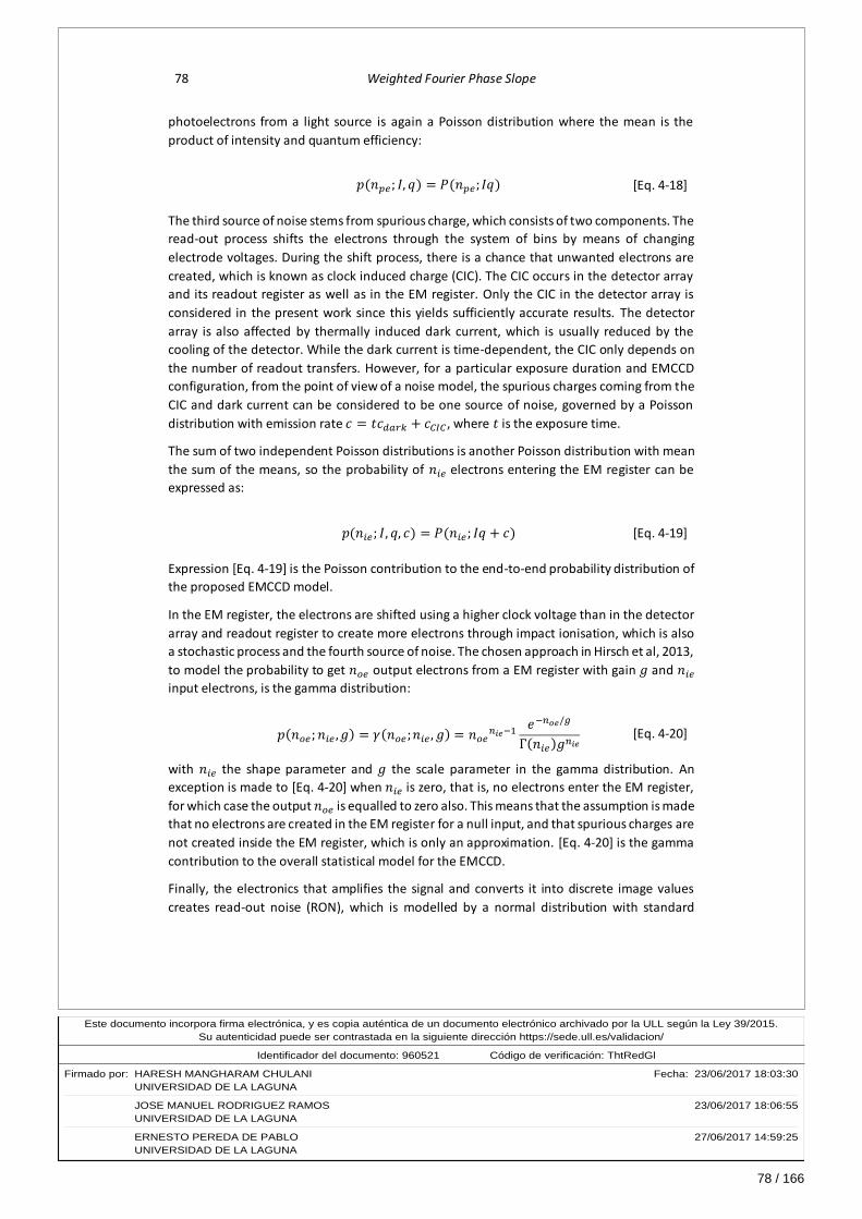
78 / 166
Este documento incorpora firma electrónica, y es copia auténtica de un documento electrónico archivado por la ULL según la Ley 39/2015.Su autenticidad puede ser contrastada en la siguiente dirección https://sede.ull.es/validacion/
Identificador del documento: 960521Código de verificación: ThtRedGl
Firmado por: HARESH MANGHARAM CHULANI Fecha: 23/06/2017 18:03:30UNIVERSIDAD DE LA LAGUNA
JOSE MANUEL RODRIGUEZ RAMOS 23/06/2017 18:06:55UNIVERSIDAD DE LA LAGUNA
ERNESTO PEREDA DE PABLO 27/06/2017 14:59:25UNIVERSIDAD DE LA LAGUNA
78 Weighted Fourier Phase Slope
photoelectrons from a light source is again a Poisson distribution where the mean is the
product of intensity and quantum efficiency:
𝑝(𝑛𝑝𝑒; 𝐼, 𝑞) = 𝑃(𝑛𝑝𝑒; 𝐼𝑞) [Eq. 4-18]
The third source of noise stems from spurious charge, which consists of two components. The
read-out process shifts the electrons through the system of bins by means of changing
electrode voltages. During the shift process, there is a chance that unwanted electrons are
created, which is known as clock induced charge (CIC). The CIC occurs in the detector array
and its readout register as well as in the EM register. Only the CIC in the detector array is
considered in the present work since this yields sufficiently accurate results. The detector
array is also affected by thermally induced dark current, which is usually reduced by the
cooling of the detector. While the dark current is time-dependent, the CIC only depends on
the number of readout transfers. However, for a particular exposure duration and EMCCD
configuration, from the point of view of a noise model, the spurious charges coming from the
CIC and dark current can be considered to be one source of noise, governed by a Poisson
distribution with emission rate 𝑐 = 𝑡𝑐𝑑𝑎𝑟𝑘 + 𝑐𝐶𝐼𝐶, where 𝑡 is the exposure time.
The sum of two independent Poisson distributions is another Poisson distribution with mean
the sum of the means, so the probability of 𝑛𝑖𝑒 electrons entering the EM register can be
expressed as:
𝑝(𝑛𝑖𝑒; 𝐼, 𝑞, 𝑐) = 𝑃(𝑛𝑖𝑒; 𝐼𝑞 + 𝑐) [Eq. 4-19]
Expression [Eq. 4-19] is the Poisson contribution to the end-to-end probability distribution of
the proposed EMCCD model.
In the EM register, the electrons are shifted using a higher clock voltage than in the detector
array and readout register to create more electrons through impact ionisation, which is also
a stochastic process and the fourth source of noise. The chosen approach in Hirsch et al, 2013,
to model the probability to get 𝑛𝑜𝑒 output electrons from a EM register with gain 𝑔 and 𝑛𝑖𝑒
input electrons, is the gamma distribution:
𝑝(𝑛𝑜𝑒; 𝑛𝑖𝑒 , 𝑔) = 𝛾(𝑛𝑜𝑒;𝑛𝑖𝑒 , 𝑔) = 𝑛𝑜𝑒𝑛𝑖𝑒−1
𝑒−𝑛𝑜𝑒/𝑔
Γ(𝑛𝑖𝑒)𝑔𝑛𝑖𝑒
[Eq. 4-20]
with 𝑛𝑖𝑒 the shape parameter and 𝑔 the scale parameter in the gamma distribution. An
exception is made to [Eq. 4-20] when 𝑛𝑖𝑒 is zero, that is, no electrons enter the EM register,
for which case the output 𝑛𝑜𝑒 is equalled to zero also. This means that the assumption is made
that no electrons are created in the EM register for a null input, and that spurious charges are
not created inside the EM register, which is only an approximation. [Eq. 4-20] is the gamma
contribution to the overall statistical model for the EMCCD.
Finally, the electronics that amplifies the signal and converts it into discrete image values
creates read-out noise (RON), which is modelled by a normal distribution with standard
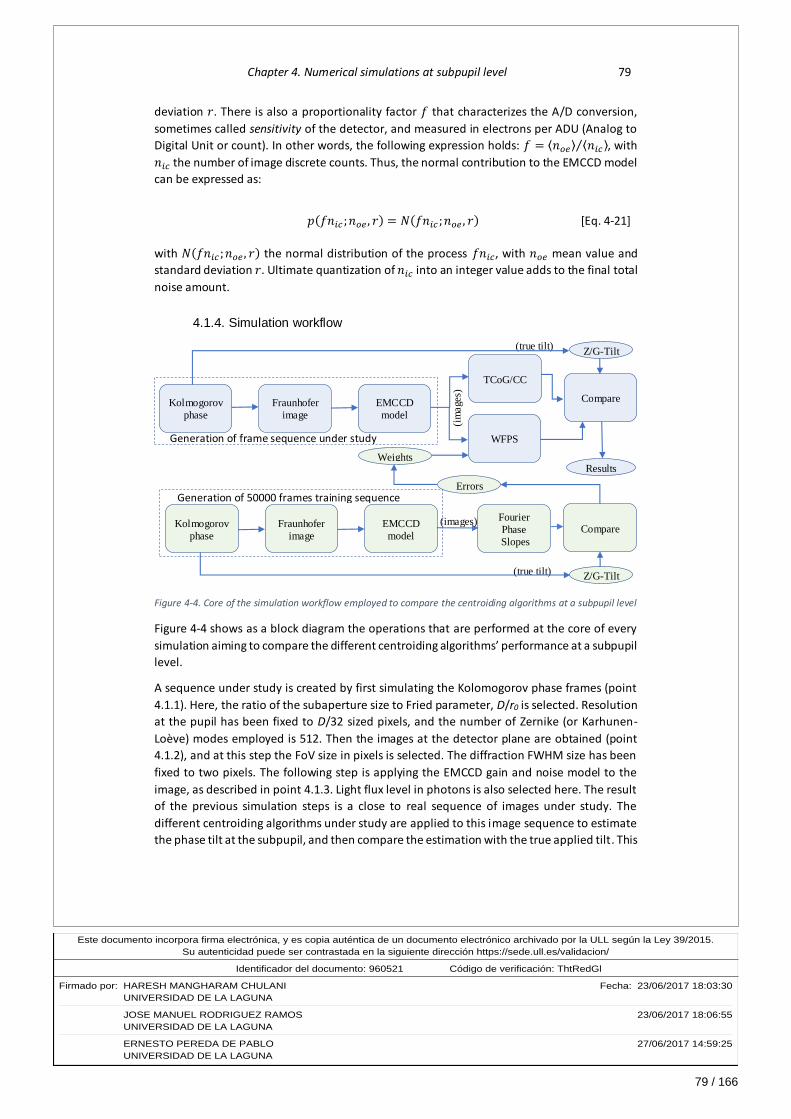
79 / 166
Este documento incorpora firma electrónica, y es copia auténtica de un documento electrónico archivado por la ULL según la Ley 39/2015.Su autenticidad puede ser contrastada en la siguiente dirección https://sede.ull.es/validacion/
Identificador del documento: 960521Código de verificación: ThtRedGl
Firmado por: HARESH MANGHARAM CHULANI Fecha: 23/06/2017 18:03:30UNIVERSIDAD DE LA LAGUNA
JOSE MANUEL RODRIGUEZ RAMOS 23/06/2017 18:06:55UNIVERSIDAD DE LA LAGUNA
ERNESTO PEREDA DE PABLO 27/06/2017 14:59:25UNIVERSIDAD DE LA LAGUNA
Chapter 4. Numerical simulations at subpupil level 79
deviation 𝑟. There is also a proportionality factor 𝑓 that characterizes the A/D conversion,
sometimes called sensitivity of the detector, and measured in electrons per ADU (Analog to
Digital Unit or count). In other words, the following expression holds: 𝑓 = ⟨𝑛𝑜𝑒⟩ ⟨𝑛𝑖𝑐⟩⁄ , with
𝑛𝑖𝑐 the number of image discrete counts. Thus, the normal contribution to the EMCCD model
can be expressed as:
𝑝(𝑓𝑛𝑖𝑐 ;𝑛𝑜𝑒 , 𝑟) = 𝑁(𝑓𝑛𝑖𝑐 ;𝑛𝑜𝑒 , 𝑟) [Eq. 4-21]
with 𝑁(𝑓𝑛𝑖𝑐 ;𝑛𝑜𝑒 , 𝑟) the normal distribution of the process 𝑓𝑛𝑖𝑐, with 𝑛𝑜𝑒 mean value and
standard deviation 𝑟. Ultimate quantization of 𝑛𝑖𝑐 into an integer value adds to the final total
noise amount.
4.1.4. Simulation workflow
Figure 4-4. Core of the simulation workflow employed to compare the centroiding algorithms at a subpupil level
Figure 4-4 shows as a block diagram the operations that are performed at the core of every
simulation aiming to compare the different centroiding algorithms’ performance at a subpupil
level.
A sequence under study is created by first simulating the Kolomogorov phase frames (point
4.1.1). Here, the ratio of the subaperture size to Fried parameter, D/r0 is selected. Resolution
at the pupil has been fixed to D/32 sized pixels, and the number of Zernike (or Karhunen-
Loève) modes employed is 512. Then the images at the detector plane are obtained (point
4.1.2), and at this step the FoV size in pixels is selected. The diffraction FWHM size has been
fixed to two pixels. The following step is applying the EMCCD gain and noise model to the
image, as described in point 4.1.3. Light flux level in photons is also selected here. The result
of the previous simulation steps is a close to real sequence of images under study. The
different centroiding algorithms under study are applied to this image sequence to estimate
the phase tilt at the subpupil, and then compare the estimation with the true applied tilt. This
(im
age
s)
(true tilt)
(true tilt)
Generation of 50000 frames training sequence
Generation of frame sequence under study
(images)
Kolmogorov
phase
Fraunhofer
image
EMCCD
model
TCoG/CC
WFPS
Z/G-Tilt
Compare
Results
Kolmogorov
phase
Fraunhofer
image
EMCCD
model
Z/G-Tilt
Fourier
Phase
Slopes
Weights
Errors
Compare

80 / 166
Este documento incorpora firma electrónica, y es copia auténtica de un documento electrónico archivado por la ULL según la Ley 39/2015.Su autenticidad puede ser contrastada en la siguiente dirección https://sede.ull.es/validacion/
Identificador del documento: 960521Código de verificación: ThtRedGl
Firmado por: HARESH MANGHARAM CHULANI Fecha: 23/06/2017 18:03:30UNIVERSIDAD DE LA LAGUNA
JOSE MANUEL RODRIGUEZ RAMOS 23/06/2017 18:06:55UNIVERSIDAD DE LA LAGUNA
ERNESTO PEREDA DE PABLO 27/06/2017 14:59:25UNIVERSIDAD DE LA LAGUNA
80 Weighted Fourier Phase Slope
true tilt can be the Zernike tilt (Z-Tilt), which was obtained at the first step of the simulation,
or the G-Tilt, which is obtained by applying a true CoG to a version of the image sequence
with maximum FoV and exempt of noise.
A parallel training sequence, with 50000 frames and with exactly the same system parameters
as the sequence under study, is simulated in order to obtain the necessary weights for the
WFPS algorithm. The Fourier phase slopes of the sequence at a set of spatial frequencies are
obtained by applying [Eq. 3-15] to each image, and the resulting spot’s displacement
measurements are compared to the true applied phase tilt to obtain the measurement errors.
MAP weights are a function of the measurement error covariance matrix, as expressed in [Eq.
3-22]. The number and order of the spatial frequencies involved in the WFPS algorithm, and
consequently the number of weights, are selectable in the simulation.
As for the control algorithms, TCoG’s threshold is a unique value for the whole sequence
under study, and is calculated by minimizing the tilt estimation error of the whole sequence
under study itself. For the CC algorithm, the reference image is a bi-dimensional Gaussian
shape for which the FWHM and the spanned FoV are selectable parameters. The correlation
figure is obtained with no interpolation, i.e., with the same resolution as the live and
reference images. The centroid is calculated over the correlation figure with a TCoG
algorithm, for which the threshold is again a unique value for the whole sequence and is
calculated by minimization of the final tilt estimation error for the whole sequence under
study.
The centroiding algorithms give the result of spot’s displacement in pixel units. In order to
compare their outputs with the system’s input phase tilt and to give the final estimation errors
in wave radians at the sensing wavelength, a conversion from displacement in pixels to wave
radians becomes mandatory. Expression [Eq. 1-13] was obtained through geometrical
considerations and relates displacement in pixels 𝑑′ with the peak to valley phase tilt Δϕ
across the subaperture width at the telescope’s pupil plane Δ𝑥:
Δϕ
Δ𝑥= [2𝜋
𝜆
𝑓
𝐹
𝑑𝑝𝑖𝑥𝑓𝜇𝑙] 𝑑′ [Eq. 4-22]
with 𝐹/𝑓 the magnification factor of the phase tilt from the telescope’s aperture to the
SHWFS’s input, and 𝑑𝑝𝑖𝑥/𝑓𝜇𝑙 the angular pixel size. Taking into account that the size of the
SHWFS’s subaperture 𝐷 is 𝐷 = Δ𝑥𝑓/𝐹, and substituting [Eq. 4-16] into [Eq. 4-22], we get:
Δϕ = [2𝜋𝑁𝑝𝑁𝑓𝑓𝑡
] 𝑑′ [Eq. 4-23]
with 𝑁𝑝 and 𝑁𝑓𝑓𝑡 the simulation parameters corresponding to the number of pixels in one
dimension in the subpupil’s domain and the number of pixels in one dimension for the
maximum FoV in the image domain, respectively. Finally, with the aim of giving the estimation
error results in r.m.s. radians, peak to valley tilt is divided by a factor of four when the
subaperture is circular, resulting in:

81 / 166
Este documento incorpora firma electrónica, y es copia auténtica de un documento electrónico archivado por la ULL según la Ley 39/2015.Su autenticidad puede ser contrastada en la siguiente dirección https://sede.ull.es/validacion/
Identificador del documento: 960521Código de verificación: ThtRedGl
Firmado por: HARESH MANGHARAM CHULANI Fecha: 23/06/2017 18:03:30UNIVERSIDAD DE LA LAGUNA
JOSE MANUEL RODRIGUEZ RAMOS 23/06/2017 18:06:55UNIVERSIDAD DE LA LAGUNA
ERNESTO PEREDA DE PABLO 27/06/2017 14:59:25UNIVERSIDAD DE LA LAGUNA
Chapter 4. Numerical simulations at subpupil level 81
Δϕ𝑟𝑚𝑠 = [𝜋
2
𝑁𝑝𝑁𝑓𝑓𝑡
]𝑑′ [Eq. 4-24]
with 𝑁𝑝 the number of phase pixels spanned by the aperture’s diameter. For a square
subaperture, the factor8 relating peak to valley and r.m.s. phase is 2√3, and so:
Δϕ𝑟𝑚𝑠𝑆𝑄𝑅
= [𝜋
√3
𝑁𝑝𝑁𝑓𝑓𝑡
] 𝑑′ [Eq. 4-25]
with 𝑁𝑝 the number of phase pixels spanned by the aperture’s side.
As an example, the true horizontal Z-tilt, given in r.m.s. wave radians at the sensing
wavelength, for a circular subaperture, is the coefficient of the second Zernike function in the
phase Zernike expansion, 𝑐2 in [Eq. 4-3]. For a given estimated horizontal spot’s displacement
�̂�′𝑥, given in pixels, and obtained by any of the centroiding methods, the estimated horizontal
Z-tilt in r.m.s. radians would be �̂�2 = �̂�′𝑥(𝜋/2)(𝑁𝑝/𝑁𝑓𝑓𝑡).
4.2. Linearity and dynamic range
One of the main concerns regarding centroiding algorithms is their linearity when operation
in large dynamic ranges is required. Some illustrations are shown in this section that compare
the WFPS with other algorithms in this respect. Open loop observation is assumed with a large
subaperture size to Fried parameter ratio (D/r0=2.5) so that the spot’s tilt excursion, and
hence the required dynamic range, are large.
Figure 4-5 shows the estimated Z-Tilt, in r.m.s. radians at the sensing wavelength, as a
function of applied Z-Tilt and the FoV extent in pixels by pixels for the WFPS algorithm (a) and
the TCoG algorithm (b), for a circular subaperture with D/r0=2.5, Nyquist sampling (FWHM at
diffraction of 2 pixels), high light flux level of 500000 photons, QE value of 97%, unity EMCCD
gain, CIC noise of 0.05 e-/pixel/frame, RON noise of 50 e- r.m.s. and sensitivity of 10 e-/ADU.9
Non-smooth aspect of the graphs is due to the spot’s deformation in response to high order
aberrations in the atmospheric turbulence, and not because of detector noises, which are
negligible with respect to the light flux level. Response is plotted up to an absolute value of 5
r.m.s. radians of applied tilt across the subaperture, which correspond to 6.37 pixels of spot’s
displacement, according to equation [Eq. 4-24]. Recovered Z-Tilt shows a very good linearity
for FoV’s of 16 x 16 and 14 x 14 pixels, for both algorithms. It only starts worsening when the
FoV is reduced to 12 x 12 pixels, at both extremes of the graph, for applied tilts greater (in
absolute value) than 4 r.m.s. radians (5.1 pixels of displacement). When FoV is further reduced
to 8 x 8 pixels, linearity is only maintained up to 2 r.m.s. radians of applied tilt. TCoG algorithm
can even completely lose the tilt estimation for applied tilts close to 5 r.m.s. radians, when
8 This factor has been derived by the author 9 Unless otherwise stated, simulations in this section are for a Nyquist sampled spot (FWHM at diffraction of 2
pixels) and typical values of detector parameters: RON of 50 e- r.m.s., CIC of 0.05 e-/pixel/frame, QE of 97% (which is the Andor Ixon 860 EMCCD response at wavelengths between 500 and 600 nm), and sensitivity of 10 e-/ADU.

82 / 166
Este documento incorpora firma electrónica, y es copia auténtica de un documento electrónico archivado por la ULL según la Ley 39/2015.Su autenticidad puede ser contrastada en la siguiente dirección https://sede.ull.es/validacion/
Identificador del documento: 960521Código de verificación: ThtRedGl
Firmado por: HARESH MANGHARAM CHULANI Fecha: 23/06/2017 18:03:30UNIVERSIDAD DE LA LAGUNA
JOSE MANUEL RODRIGUEZ RAMOS 23/06/2017 18:06:55UNIVERSIDAD DE LA LAGUNA
ERNESTO PEREDA DE PABLO 27/06/2017 14:59:25UNIVERSIDAD DE LA LAGUNA
82 Weighted Fourier Phase Slope
the spot almost gets out of the observed FoV and only its tail remains inside. WFPS, however,
has the capacity to keep up with the estimation, as long as the tail’s intensity is over the
background noise (see point A.5.2 for an example that explains this behaviour).
The reason for such a good linearity behaviour of both algorithms when the FoV is adequate
is that, for a high light flux level, the TCoG makes use of the threshold to eliminate the tails of
the spot and concentrate in the central more symmetric part of the spot, thereby correctly
estimating the Z-Tilt even when the spot may be slightly truncated. WFPS, on the other hand,
overcomes spot’s truncation by giving very small weight to the zero spatial frequency and
larger weights to other frequencies that are less affected by spot’s truncation.
Figure 4-5. (a) Estimated Z-Tilt as a function of applied Z-Tilt and FoV, for the WFPS algorithm with 4 x 4 spatial frequencies, circular subaperture with D/r0=2.5, Nyquist sampling, high light flux level of 500000 photons, unity
EMCCD gain, CIC=0.05 e-/pixel/frame, RON=50 e-r.m.s. (b) Same for the TCoG algorithm.
Figure 4-6 shows the result of a repetition of the previous experiment, maintaining all the
system’s parameters, with the only difference that G-Tilt is estimated. Both algorithms see
their linearity worsened, even for the largest 16 x 16 pixels FoV. This is because G-Tilt is

83 / 166
Este documento incorpora firma electrónica, y es copia auténtica de un documento electrónico archivado por la ULL según la Ley 39/2015.Su autenticidad puede ser contrastada en la siguiente dirección https://sede.ull.es/validacion/
Identificador del documento: 960521Código de verificación: ThtRedGl
Firmado por: HARESH MANGHARAM CHULANI Fecha: 23/06/2017 18:03:30UNIVERSIDAD DE LA LAGUNA
JOSE MANUEL RODRIGUEZ RAMOS 23/06/2017 18:06:55UNIVERSIDAD DE LA LAGUNA
ERNESTO PEREDA DE PABLO 27/06/2017 14:59:25UNIVERSIDAD DE LA LAGUNA
Chapter 4. Numerical simulations at subpupil level 83
correctly estimated by a pure CoG. So TCoG’s optimal threshold is zero or close by, and WFPS
tends to give a high weight to zero spatial frequency. In both cases, truncation of the spot
affects the estimated G-Tilt. In any case, overall behaviour of both algorithms with respect to
linearity when estimating G-Tilt is again very similar.
Figure 4-6. (a) Estimated G-Tilt as a function of applied G-Tilt and FoV, for the WFPS algorithm with 4 x 4 spatial frequencies, circular subaperture with D/r0=2.5, Nyquist sampling, high light flux level of 500000 photons, unity EMCCD gain, CIC=0.05 e-/pixel/frame, RON=50 e-r.m.s. (b) Same for the TCoG algorithm.
Figure 4-7 concentrates on the particular case of a FoV of 8 x 8 pixels, for a system with the
same parameters as the previous simulations, and for estimation of Z-Tilt (a) and G-Tilt (b)
with TCoG, CC, WFPS and a version of WFPS that employs 16 x 16 2D-FFT’s. CC algorithm
employs a 2D Gaussian reference with FWHM of 2 pixels, FoV of 8 pixels, and no interpolation.
Centroid is computed by a TCoG over the correlation figure.10 A very similar behaviour can be
seen between the CC and TCoG algorithms. The WFPS with augmented 2D-FFT size has the
10 Unless otherwise stated, the CC algorithm will employ a 2D Gaussian as a reference, with FWHM=2 pixels, FoV=8pixels, and no interpolation. Centroid is computed by a TCoG over the correlation figure.

84 / 166
Este documento incorpora firma electrónica, y es copia auténtica de un documento electrónico archivado por la ULL según la Ley 39/2015.Su autenticidad puede ser contrastada en la siguiente dirección https://sede.ull.es/validacion/
Identificador del documento: 960521Código de verificación: ThtRedGl
Firmado por: HARESH MANGHARAM CHULANI Fecha: 23/06/2017 18:03:30UNIVERSIDAD DE LA LAGUNA
JOSE MANUEL RODRIGUEZ RAMOS 23/06/2017 18:06:55UNIVERSIDAD DE LA LAGUNA
ERNESTO PEREDA DE PABLO 27/06/2017 14:59:25UNIVERSIDAD DE LA LAGUNA
84 Weighted Fourier Phase Slope
capacity to slightly improve linearity with respect to TCoG. For example, a 6% improvement
is seen when estimating Z-Tilt with 3 rms radians applied.
Figure 4-7. (a) Estimated Z-Tilt as a function of applied Z-Tilt and centroiding algorithm, for a FoV of 8 x 8 pixels, circular subaperture with D/r0=2.5, Nyquist sampling, high light flux level of 500000 photons, unity EMCCD
gain, CIC=0.05 e-/pixel/frame, RON=50 e-r.m.s. (b) Same for G-Tilt estimation.
4.2.1. Optimum field of view
A question that naturally arises is what field of view or dynamic range would be the optimum
in every situation, and this depends on the turbulence strength, the light flux level and the
robustness of the centroiding algorithm against detector noise. Turbulence strength calls for
large FoV’s so that linearity is maintained, as it has just been explained. On the other hand,
as the signal to noise ratio gets lower, lower FoV’s will be preferred in order to reduce noisy
pixels. This will be truer for those centroiding algorithms which are more affected by the
detector’s noises.

85 / 166
Este documento incorpora firma electrónica, y es copia auténtica de un documento electrónico archivado por la ULL según la Ley 39/2015.Su autenticidad puede ser contrastada en la siguiente dirección https://sede.ull.es/validacion/
Identificador del documento: 960521Código de verificación: ThtRedGl
Firmado por: HARESH MANGHARAM CHULANI Fecha: 23/06/2017 18:03:30UNIVERSIDAD DE LA LAGUNA
JOSE MANUEL RODRIGUEZ RAMOS 23/06/2017 18:06:55UNIVERSIDAD DE LA LAGUNA
ERNESTO PEREDA DE PABLO 27/06/2017 14:59:25UNIVERSIDAD DE LA LAGUNA
Chapter 4. Numerical simulations at subpupil level 85
Figure 4-8. Tilt estimation error in r.m.s. radians as a function of FoV and light flux level for the TCoG algorithm
(red), the CC algorithm (green) and the WFPS algorithm with 4 x 4 spatial frequencies (blue), for Z-Tilt estimation (a) and G-Tilt estimation (b). D/r0 is 2.5. CIC is 0.05 e-/pix/frame and RON is 50 e- rms.
Optimal FoV for Z-Tilt/G-Tilt estimation (pixels x pixels). D/r0=2.5
#photons (per subpupil)
TCoG CC WFPS
(4x4 freqs)
10 10x10/10x10 10x10/10x10 10x10/10x10 20 10x10/10x10 10x10/12x12 12x12/12x12 30 10x10/10x10 12x12/12x12 12x12/12x12 50 12x12/12x12 12x12/12x12 14x14/16x16 100 12x12/12x12 16x16/12x12 16x16/16x16 300 14x14/16x16 16x16/16x16 16x16/16x16 10000 16x16/16x16 16x16/16x16 16x16/16x16
Table 4-2. Optimal FoV in pixels x pixels as a function of light flux level for the TCoG, CC and WFPS (with 4x4 frequencies) algorithms, obtained from Figure 4-8. D/r0=2.5. CIC=0.05 e-/pix/frame. RON=50 e- rms.
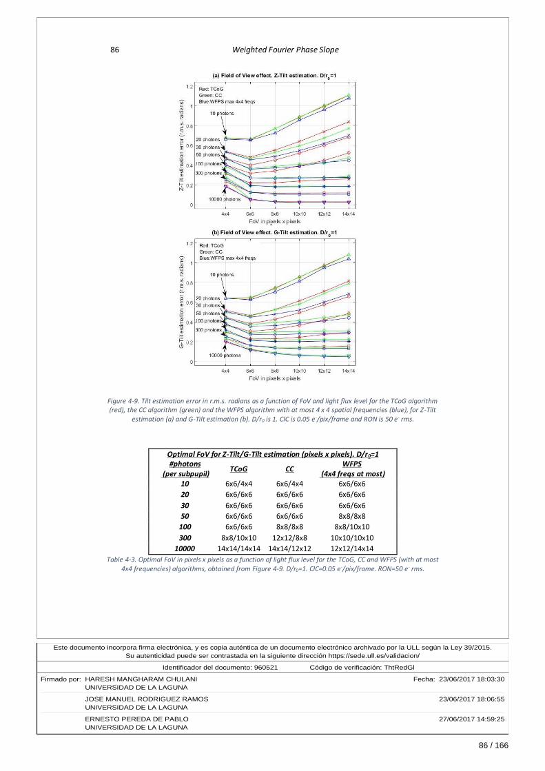
86 / 166
Este documento incorpora firma electrónica, y es copia auténtica de un documento electrónico archivado por la ULL según la Ley 39/2015.Su autenticidad puede ser contrastada en la siguiente dirección https://sede.ull.es/validacion/
Identificador del documento: 960521Código de verificación: ThtRedGl
Firmado por: HARESH MANGHARAM CHULANI Fecha: 23/06/2017 18:03:30UNIVERSIDAD DE LA LAGUNA
JOSE MANUEL RODRIGUEZ RAMOS 23/06/2017 18:06:55UNIVERSIDAD DE LA LAGUNA
ERNESTO PEREDA DE PABLO 27/06/2017 14:59:25UNIVERSIDAD DE LA LAGUNA
86 Weighted Fourier Phase Slope
Figure 4-9. Tilt estimation error in r.m.s. radians as a function of FoV and light flux level for the TCoG algorithm (red), the CC algorithm (green) and the WFPS algorithm with at most 4 x 4 spatial frequencies (blue), for Z-Tilt
estimation (a) and G-Tilt estimation (b). D/r0 is 1. CIC is 0.05 e-/pix/frame and RON is 50 e- rms.
Optimal FoV for Z-Tilt/G-Tilt estimation (pixels x pixels). D/r0=1
#photons (per subpupil)
TCoG CC WFPS
(4x4 freqs at most)
10 6x6/4x4 6x6/4x4 6x6/6x6 20 6x6/6x6 6x6/6x6 6x6/6x6 30 6x6/6x6 6x6/6x6 6x6/6x6 50 6x6/6x6 6x6/6x6 8x8/8x8 100 6x6/6x6 8x8/8x8 8x8/10x10 300 8x8/10x10 12x12/8x8 10x10/10x10 10000 14x14/14x14 14x14/12x12 12x12/14x14
Table 4-3. Optimal FoV in pixels x pixels as a function of light flux level for the TCoG, CC and WFPS (with at most
4x4 frequencies) algorithms, obtained from Figure 4-9. D/r0=1. CIC=0.05 e-/pix/frame. RON=50 e- rms.

87 / 166
Este documento incorpora firma electrónica, y es copia auténtica de un documento electrónico archivado por la ULL según la Ley 39/2015.Su autenticidad puede ser contrastada en la siguiente dirección https://sede.ull.es/validacion/
Identificador del documento: 960521Código de verificación: ThtRedGl
Firmado por: HARESH MANGHARAM CHULANI Fecha: 23/06/2017 18:03:30UNIVERSIDAD DE LA LAGUNA
JOSE MANUEL RODRIGUEZ RAMOS 23/06/2017 18:06:55UNIVERSIDAD DE LA LAGUNA
ERNESTO PEREDA DE PABLO 27/06/2017 14:59:25UNIVERSIDAD DE LA LAGUNA
Chapter 4. Numerical simulations at subpupil level 87
Figure 4-8 shows the dependence of the tilt estimation error in r.m.s. radians at the sensing
wavelength with the FoV in pixels by pixels and light flux level in photons, for the TCoG
algorithm (red lines), the CC algorithm (green lines) and the WFPS algorithm with 4x4 spatial
frequencies (blue lines), when estimating Z-Tilt (a) and estimating G-Tilt (b). D/r0 is 2.5. CIC is
0.05 e-/pix/frame and RON is 50 e- rms. Selected EM gain for each light level is high without
saturating a 14 bits detector. Table 4-2 collects the optimal FoV values for the different light
flux levels and the three algorithms under study. A general conclusion that can be extracted
from this simulation is that the WFPS algorithm is the least affected by detector noise among
the three evaluated algorithms, calling for bigger FoV’s for each light level under study, and
giving as a result a better tilt estimation at the optimal FoV. CC algorithm would be in the
second place in this respect, with a very similar behaviour. However, TCoG is very much
affected by detector noise, and requires small optimal FoV’s. Moreover, red traces in Figure
4-8 tend to rapidly increase with FoV value for light levels below 100 photons, indicating that
TCoG algorithm is very sensitive to the optimal selection of FoV. WFPS and CC are much more
tolerant in this sense, allowing for a broader range of FoV selection with little or no
penalization in tilt estimation error for light levels above 30 photons. For low light level such
as 30 to 50 photons, TCoG must work with FoV’s in the order of 10x10 to 12x12 pixels,
whereas CC and WFPS can work with FoV’s of 12x12 to even 16x16 pixels.
Figure 4-9 and Table 4-3 illustrate the result for an identical simulation for D/r0=1. The WFPS
employs 2 x 2 spatial frequencies for the 4 x 4 pixels FoV, 3 x 3 spatial frequencies for the 6 x
6 pixels FoV, and 4 x 4 spatial frequencies for the rest of FoV values. Very similar conclusions
to the previous simulations can be extracted. TCoG requires as low a FoV as 6x6 pixels for
light levels of 100 photons and below, whereas CC and WFPS work better with higher FoV’s
of 8x8 or 10x10 pixels for 50 photons of incident light or above.
4.3. MAP weights
Once the working FoV is decided, we are in a position to determine the number of spatial
frequencies to involve in the WFPS algorithm and the value of their corresponding MAP
weights. The number of spatial frequencies has a direct impact on the computational cost of
the algorithm, as seen in point 3.3.2 (see Tables 3-1 and 3-2), and a certain impact on the tilt
estimation error, as will be seen in the present point.
Note here that the numerical simulation of the system at a subpupil level is a must in order
to obtain the necessary MAP weights for the WFPS algorithm. These weights are a function
of the tilt estimation error covariance matrices 𝑉𝐸𝑥 and 𝑉𝐸𝑦 as expressed in [Eq. 3-22], with
tilt estimation error vectors 𝐸𝑥 and 𝐸𝑦 defined in [Eq. 3-18]. These error covariance matrices
can only be determined when a sufficiently large set of input phases to the system and their
corresponding recovered phase tilts at the involved spatial frequencies are known, and this is
only feasible through numerical simulation. This is the reason why, for every simulation
performed in this chapter and for every sequence of turbulent phases under study, a parallel
much larger sequence of 50000 frames with the same system parameters is always utilized to
obtain the error covariance matrices and thereby the MAP weights for the WFPS algorithm,
as shown in the simulation workflow in Figure 4-4.
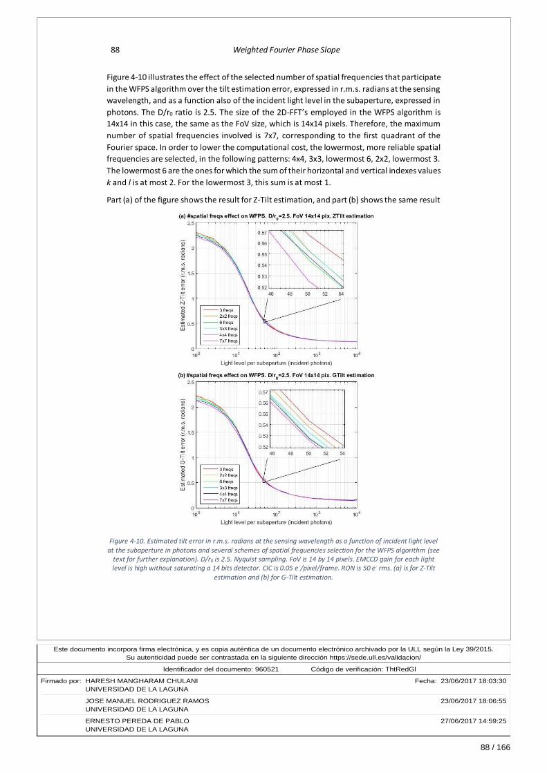
88 / 166
Este documento incorpora firma electrónica, y es copia auténtica de un documento electrónico archivado por la ULL según la Ley 39/2015.Su autenticidad puede ser contrastada en la siguiente dirección https://sede.ull.es/validacion/
Identificador del documento: 960521Código de verificación: ThtRedGl
Firmado por: HARESH MANGHARAM CHULANI Fecha: 23/06/2017 18:03:30UNIVERSIDAD DE LA LAGUNA
JOSE MANUEL RODRIGUEZ RAMOS 23/06/2017 18:06:55UNIVERSIDAD DE LA LAGUNA
ERNESTO PEREDA DE PABLO 27/06/2017 14:59:25UNIVERSIDAD DE LA LAGUNA
88 Weighted Fourier Phase Slope
Figure 4-10 illustrates the effect of the selected number of spatial frequencies that participate
in the WFPS algorithm over the tilt estimation error, expressed in r.m.s. radians at the sensing
wavelength, and as a function also of the incident light level in the subaperture, expressed in
photons. The D/r0 ratio is 2.5. The size of the 2D-FFT’s employed in the WFPS algorithm is
14x14 in this case, the same as the FoV size, which is 14x14 pixels. Therefore, the maximum
number of spatial frequencies involved is 7x7, corresponding to the first quadrant of the
Fourier space. In order to lower the computational cost, the lowermost, more reliable spatial
frequencies are selected, in the following patterns: 4x4, 3x3, lowermost 6, 2x2, lowermost 3.
The lowermost 6 are the ones for which the sum of their horizontal and vertical indexes values
k and l is at most 2. For the lowermost 3, this sum is at most 1.
Part (a) of the figure shows the result for Z-Tilt estimation, and part (b) shows the same result
Figure 4-10. Estimated tilt error in r.m.s. radians at the sensing wavelength as a function of incident light level at the subaperture in photons and several schemes of spatial frequencies selection for the WFPS algorithm (see
text for further explanation). D/r0 is 2.5. Nyquist sampling. FoV is 14 by 14 pixels. EMCCD gain for each light level is high without saturating a 14 bits detector. CIC is 0.05 e -/pixel/frame. RON is 50 e- rms. (a) is for Z-Tilt
estimation and (b) for G-Tilt estimation.

89 / 166
Este documento incorpora firma electrónica, y es copia auténtica de un documento electrónico archivado por la ULL según la Ley 39/2015.Su autenticidad puede ser contrastada en la siguiente dirección https://sede.ull.es/validacion/
Identificador del documento: 960521Código de verificación: ThtRedGl
Firmado por: HARESH MANGHARAM CHULANI Fecha: 23/06/2017 18:03:30UNIVERSIDAD DE LA LAGUNA
JOSE MANUEL RODRIGUEZ RAMOS 23/06/2017 18:06:55UNIVERSIDAD DE LA LAGUNA
ERNESTO PEREDA DE PABLO 27/06/2017 14:59:25UNIVERSIDAD DE LA LAGUNA
Chapter 4. Numerical simulations at subpupil level 89
MAP weights for WFPS horizontal centroid (𝑾𝒌,𝒍𝒙 ). Z-Tilt estimation.
D/r0=2.5. FoV=14x14 pixels.
Photons 3 frequencies 6 frequencies 4 x 4 frequencies
10
0.9265 0.0350 0.0000 0.0000 0.9330 0.0314 -0.0227 0.0000 1.0019 0.0336 -0.0214 -0.0101
0.0386 0.0409 0.0189 0.0440 0.0210 -0.0001 -0.0082 -0.0014 0.0033 -0.0027 -0.0045 -0.0103 -0.0098 -0.0099 -0.0124 -0.0144
20
0.7850 0.0956 0.7166 0.0860 0.0048 0.7224 0.0870 0.0030 -0.0025 0.1194 0.1238 0.0535 0.1163 0.0526 0.0116 -0.0011 0.0152 0.0133 0.0084 0.0047 -0.0039
-0.0009 -0.0009 -0.0029 -0.0071
30
0.6573 0.1532 0.5636 0.1390 0.0232 0.5385 0.1339 0.0192 0.0029
0.1895 0.1854 0.0680 0.1828 0.0674 0.0167 0.0029 0.0207 0.0184 0.0092 0.0063 -0.0004 0.0024 0.0033 -0.0001 -0.0035
50
0.5455 0.2250 0.4560 0.1996 0.0294 0.4326 0.1891 0.0286 0.0046 0.2296 0.2337 0.0646 0.2191 0.0629 0.0161 0.0060 0.0168 0.0159 0.0102 0.0073 0.0016
0.0042 0.0030 0.0011 -0.0023
100
0.4442 0.3029 0.4050 0.2669 0.0306 0.3801 0.2564 0.0255 0.0077
0.2530 0.2399 0.0426 0.2280 0.0371 0.0139 0.0071 0.0150 0.0118 0.0085 0.0077 0.0037 0.0064 0.0048 0.0017 -0.0005
200
0.3772 0.3394 0.3600 0.3088 0.0247 0.3378 0.2848 0.0196 0.0109 0.2834 0.2702 0.0238 0.2559 0.0186 0.0112 0.0088 0.0125 0.0109 0.0120 0.0090 0.0045 0.0054 0.0056 0.0040 0.0010
500
0.2885 0.3592 0.2910 0.3414 0.0178 0.2772 0.3123 0.0098 0.0128
0.3523 0.3359 0.0063 0.3210 0.0046 0.0090 0.0098 0.0077 0.0018 0.0081 0.0090 0.0063 0.0067 0.0058 0.0051 0.0007
1000
0.2468 0.3702 0.2497 0.3594 0.0134 0.2475 0.3295 0.0058 0.0127 0.3830 0.3719 0.0005 0.3485 -0.0083 0.0104 0.0095 0.0050 0.0009 0.0114 0.0103 0.0061 0.0036 0.0050 0.0049 0.0022
10000
0.2055 0.3601 0.2000 0.3517 0.0120 0.1987 0.3211 0.0050 0.0113
0.4343 0.4428 -0.0047 0.4190 -0.0062 0.0081 0.0120 -0.0018 -0.0071 0.0074 0.0096 0.0078 0.0020 0.0056 0.0046 0.0010
Table 4-4. List of MAP weights for the calculation of the horizontal value of the centroid with the WFPS
algorithm, as per [Eq. 3-23] (𝑊𝑘,𝑙𝑥 ), when estimating Z-Tilt. D/r0 is 2.5. Nyquist sampling. FoV is 14 by 14 pixels.
EMCCD gain for each light level is high without saturating a 14 bits detector. CIC is 0.05 e -/pixel/frame. RON is
50 e- rms. Light level increases vertically in the table. Three different patterns of spatial frequencies selection are listed in a column each: 3 lowermost frequencies, 6 lowermost frequencies and 4x4 lowermost frequencies.

90 / 166
Este documento incorpora firma electrónica, y es copia auténtica de un documento electrónico archivado por la ULL según la Ley 39/2015.Su autenticidad puede ser contrastada en la siguiente dirección https://sede.ull.es/validacion/
Identificador del documento: 960521Código de verificación: ThtRedGl
Firmado por: HARESH MANGHARAM CHULANI Fecha: 23/06/2017 18:03:30UNIVERSIDAD DE LA LAGUNA
JOSE MANUEL RODRIGUEZ RAMOS 23/06/2017 18:06:55UNIVERSIDAD DE LA LAGUNA
ERNESTO PEREDA DE PABLO 27/06/2017 14:59:25UNIVERSIDAD DE LA LAGUNA
90 Weighted Fourier Phase Slope
MAP weights for WFPS horizontal centroid (𝑾𝒌,𝒍𝒙 ). G-Tilt estimation.
D/r0=2.5. FoV=14x14 pixels.
Photons 3 frequencies 6 frequencies 4 x 4 frequencies
10
0.9345 0.0305 0.0000 0.0000 0.9509 0.0288 -0.0232 0.0000 1.0194 0.0311 -0.0190 -0.0106
0.0350 0.0357 0.0122 0.0387 0.0190 -0.0018 -0.0120 -0.0045 0.0007 -0.0023 -0.0055 -0.0116 -0.0106 -0.0094 -0.0140 -0.0120
20
0.8007 0.0857 0.7443 0.0788 0.0025 0.7650 0.0755 -0.0006 -0.0028 0.1135 0.1143 0.0456 0.1078 0.0456 0.0095 -0.0012 0.0146 0.0133 0.0062 0.0027 -0.0049
-0.0015 -0.0018 -0.0041 -0.0087
30
0.6885 0.1348 0.6190 0.1220 0.0167 0.6082 0.1246 0.0163 0.0007
0.1767 0.1692 0.0563 0.1620 0.0560 0.0119 0.0014 0.0168 0.0152 0.0075 0.0039 -0.0020 0.0006 0.0003 -0.0023 -0.0045
50
0.6036 0.1928 0.5476 0.1718 0.0229 0.5328 0.1614 0.0188 0.0023 0.2036 0.1998 0.0441 0.2001 0.0493 0.0101 0.0014 0.0137 0.0119 0.0060 0.0050 0.0002
0.0012 0.0004 0.0004 -0.0014
100
0.5607 0.2202 0.5392 0.2025 0.0134 0.5337 0.2012 0.0124 0.0030
0.2192 0.2177 0.0215 0.2066 0.0177 0.0041 0.0031 0.0057 0.0050 0.0038 0.0039 0.0026 0.0015 0.0009 0.0007 -0.0004
200
0.5734 0.2025 0.5660 0.2023 0.0022 0.5670 0.1996 0.0016 0.0038 0.2241 0.2343 -0.0004 0.2268 -0.0017 -0.0012 0.0029 -0.0043 -0.0040 -0.0003 0.0018 0.0028 -0.0007 0.0004 0.0001 0.0010
500
0.6243 0.1703 0.6181 0.1908 -0.0086 0.6159 0.1906 -0.0087 0.0016
0.2054 0.2331 -0.0218 0.2327 -0.0146 -0.0042 0.0016 -0.0116 -0.0112 -0.0029 -0.0007 0.0026 -0.0024 -0.0027 0.0003 0.0021
1000
0.6825 0.1467 0.6644 0.1755 -0.0126 0.6678 0.1790 -0.0099 0.0009 0.1708 0.2127 -0.0250 0.2082 -0.0174 -0.0073 0.0001 -0.0150 -0.0132 -0.0041 -0.0013 0.0003 -0.0040 -0.0018 -0.0003 0.0030
10000
0.6385 0.1436 0.6053 0.1805 -0.0174 0.6024 0.1881 -0.0133 -0.0016
0.2180 0.2972 -0.0358 0.3081 -0.0252 -0.0073 -0.0044 -0.0298 -0.0253 -0.0077 -0.0039 0.0003 -0.0066 -0.0031 -0.0021 0.0016
Table 4-5. List of MAP weights for the calculation of the horizontal value of the centroid with the WFPS
algorithm, as per [Eq. 3-23] (𝑊𝑘,𝑙𝑥 ), when estimating G-Tilt. D/r0 is 2.5. Nyquist sampling. FoV is 14 by 14 pixels.
EMCCD gain for each light level is high without saturating a 14 bits detector. CIC is 0.05 e -/pixel/frame. RON is
50 e- rms. Light level increases vertically in the table. Three different patterns of spatial frequencies selection are listed in a column each: 3 lowermost frequencies, 6 lowermost frequencies and 4x4 lowermost frequencies.

91 / 166
Este documento incorpora firma electrónica, y es copia auténtica de un documento electrónico archivado por la ULL según la Ley 39/2015.Su autenticidad puede ser contrastada en la siguiente dirección https://sede.ull.es/validacion/
Identificador del documento: 960521Código de verificación: ThtRedGl
Firmado por: HARESH MANGHARAM CHULANI Fecha: 23/06/2017 18:03:30UNIVERSIDAD DE LA LAGUNA
JOSE MANUEL RODRIGUEZ RAMOS 23/06/2017 18:06:55UNIVERSIDAD DE LA LAGUNA
ERNESTO PEREDA DE PABLO 27/06/2017 14:59:25UNIVERSIDAD DE LA LAGUNA
Chapter 4. Numerical simulations at subpupil level 91
for G-Tilt estimation. In both cases, an order of magnitude of magnification of the plot is
necessary to appreciate the change in behaviour of the WFPS algorithm when estimating the
tilt. The magnification is done around 50 photons of incident light, and only a less than 10%
variation in tilt estimation error can be appreciated between the best and the worst case for
the Z-Tilt estimation, and less than 5% variation for the G-Tilt estimation. A good compromise
between computational cost and estimation performance that will be used throughout the
work is to utilize the lowermost 6 spatial frequencies.
Tables 4-4 and 4-5 list the MAP weights 𝑊𝑘,𝑙𝑥 for the calculation of the horizontal value of the
centroids, corresponding to the previous simulation, for the Z-Tilt and G-Tilt estimation,
respectively, and for a selected number of representative light levels and three spatial
frequencies patterns: lowermost 3, lowermost 6 and lowermost 4x4. Vertical weights are the
transpose of horizontal weights, that is, 𝑊𝑘,𝑙𝑦 = 𝑊𝑙 ,𝑘
𝑥 .
The listed weights values are just as they were obtained from the simulation applied to a
50000 frames sequence realization. They should not be taken as exact values, in the sense
that they are repeatedly obtained only within a certain error margin, when different
realizations of the 50000 frames training sequence are utilized. This error margin is of a few
percent points, less than 5%, for the largest weight values, and increases for lower values,
being 10 to 20% a common error margin for weight values around 0.01. Not only the error
margin depends upon the weight value, but also on the signal level at the particular spatial
frequency, being sometimes quite big when the spatial frequency is probably near a null of
signal. In general, it has been seen that a 50000 frames long training sequence is a good
compromise between simulation time and resources consumption and weights calculation
precision.
At very low light level, below 50 photons, weights for Z-Tilt and G-Tilt estimation tend to be
quite similar, indicating that when detector noises dominate, the error distribution
throughout the spatial frequencies is similar for both cases, regardless of the exact spot shape
and whether Z-Tilt or G-Tilt is being estimated. For light levels of 100 photons and above,
when estimating Z-Tilt, there is a clear tendency of the three lowermost frequencies to
accumulate the major portion of the total weight, with more or less equally distributed values,
and with a decreasing value for the zero spatial frequency weight as light increases. Whereas
when estimating G-Tilt, the weight at zero spatial frequency is always the dominant, and tends
to increase with increasing light level above 100 photons. This was an expected behaviour for
moderate to high light levels, when high order atmospheric turbulence effects dominate
measurement noise. The algorithm tends to distribute the weights among more spatial
frequencies when estimating Z-Tilt in order to smooth the Fourier phase and symmetrize the
spot, whereas it concentrates the weight at the zero spatial frequency when estimating G-
Tilt, for it looks for a near pure CoG calculation.
By careful study of the weights, we also find a justification to employ only the lowermost six,
as the weights beyond these tend to be of the order of 0.01 or below, thus indicating that
their contribution to the final centroid estimation is low. This is both valid for G-Tilt and for Z-
Tilt estimation, though more evident for the former due to the weight concentration at zero
spatial frequency.

92 / 166
Este documento incorpora firma electrónica, y es copia auténtica de un documento electrónico archivado por la ULL según la Ley 39/2015.Su autenticidad puede ser contrastada en la siguiente dirección https://sede.ull.es/validacion/
Identificador del documento: 960521Código de verificación: ThtRedGl
Firmado por: HARESH MANGHARAM CHULANI Fecha: 23/06/2017 18:03:30UNIVERSIDAD DE LA LAGUNA
JOSE MANUEL RODRIGUEZ RAMOS 23/06/2017 18:06:55UNIVERSIDAD DE LA LAGUNA
ERNESTO PEREDA DE PABLO 27/06/2017 14:59:25UNIVERSIDAD DE LA LAGUNA
92 Weighted Fourier Phase Slope
Finally, it is fair to mention that some effort has been made to assess the algorithm’s
performance degradation with the use of non-optimal weights. It has been seen that weights
variation of 10 to even 15% in their values leads to almost no variation in estimation
performance. This kind of tests should be further and more extensively performed.
Figure 4-11. Estimated tilt error in r.m.s. radians at the sensing wavelength as a function of incident light level at the subaperture in photons and several schemes of spatial frequencies selection for the WFPS algorithm.
D/r0 is 1. Nyquist sampling. FoV is 10 by 10 pixels. EMCCD gain for each light level is high without saturating a 14 bits detector. CIC is 0.05 e-/pixel/frame. RON is 50 e- rms. (a) is for Z-Tilt and (b) for G-Tilt estimation.
Figure 4-11 and Tables 4-6 and 4-7 show the results of a repetition of the previous simulation
for a case with D/r0=1 and a FoV of 10x10 pixels. In this case, the maximum number of spatial
frequencies involved is 5x5. Again, the employment of only the six lowermost frequencies is
a good choice, and this can be seen both from the estimation performance in the figure and
from the weights values in the tables. Also, the same considerations regarding repeatability,
error margins and performance dependence on optimal weights made for the previous case,
are valid here.
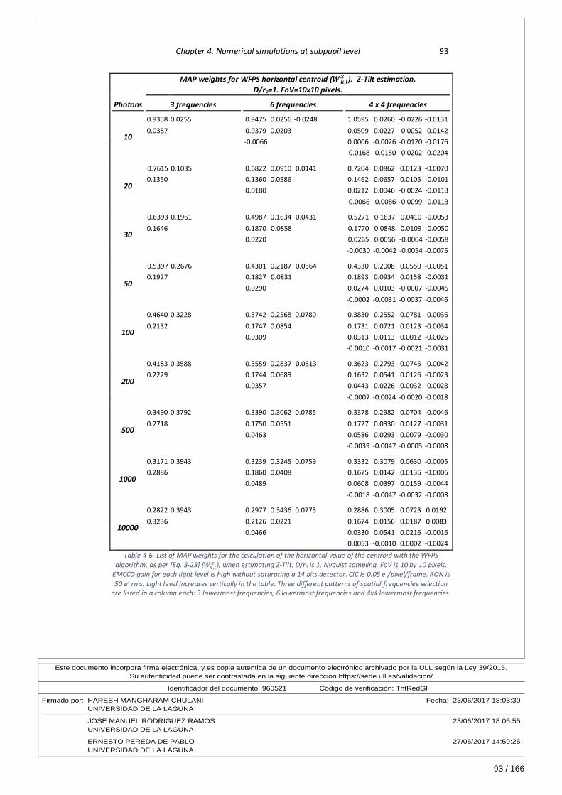
93 / 166
Este documento incorpora firma electrónica, y es copia auténtica de un documento electrónico archivado por la ULL según la Ley 39/2015.Su autenticidad puede ser contrastada en la siguiente dirección https://sede.ull.es/validacion/
Identificador del documento: 960521Código de verificación: ThtRedGl
Firmado por: HARESH MANGHARAM CHULANI Fecha: 23/06/2017 18:03:30UNIVERSIDAD DE LA LAGUNA
JOSE MANUEL RODRIGUEZ RAMOS 23/06/2017 18:06:55UNIVERSIDAD DE LA LAGUNA
ERNESTO PEREDA DE PABLO 27/06/2017 14:59:25UNIVERSIDAD DE LA LAGUNA
Chapter 4. Numerical simulations at subpupil level 93
MAP weights for WFPS horizontal centroid (𝑾𝒌,𝒍𝒙 ). Z-Tilt estimation.
D/r0=1. FoV=10x10 pixels.
Photons 3 frequencies 6 frequencies 4 x 4 frequencies
10
0.9358 0.0255 0.0000 0.0000 0.9475 0.0256 -0.0248 0.0000 1.0595 0.0260 -0.0226 -0.0131
0.0387 0.0379 0.0203 0.0509 0.0227 -0.0052 -0.0142 -0.0066 0.0006 -0.0026 -0.0120 -0.0176 -0.0168 -0.0150 -0.0202 -0.0204
20
0.7615 0.1035 0.6822 0.0910 0.0141 0.7204 0.0862 0.0123 -0.0070 0.1350 0.1360 0.0586 0.1462 0.0657 0.0105 -0.0101 0.0180 0.0212 0.0046 -0.0024 -0.0113
-0.0066 -0.0086 -0.0099 -0.0113
30
0.6393 0.1961 0.4987 0.1634 0.0431 0.5271 0.1637 0.0410 -0.0053
0.1646 0.1870 0.0858 0.1770 0.0848 0.0109 -0.0050 0.0220 0.0265 0.0056 -0.0004 -0.0058 -0.0030 -0.0042 -0.0054 -0.0075
50
0.5397 0.2676 0.4301 0.2187 0.0564 0.4330 0.2008 0.0550 -0.0051 0.1927 0.1827 0.0831 0.1893 0.0934 0.0158 -0.0031 0.0290 0.0274 0.0103 -0.0007 -0.0045
-0.0002 -0.0031 -0.0037 -0.0046
100
0.4640 0.3228 0.3742 0.2568 0.0780 0.3830 0.2552 0.0781 -0.0036
0.2132 0.1747 0.0854 0.1731 0.0721 0.0123 -0.0034 0.0309 0.0313 0.0113 0.0012 -0.0026 -0.0010 -0.0017 -0.0021 -0.0031
200
0.4183 0.3588 0.3559 0.2837 0.0813 0.3623 0.2793 0.0745 -0.0042 0.2229 0.1744 0.0689 0.1632 0.0541 0.0126 -0.0023 0.0357 0.0443 0.0226 0.0032 -0.0028 -0.0007 -0.0024 -0.0020 -0.0018
500
0.3490 0.3792 0.3390 0.3062 0.0785 0.3378 0.2982 0.0704 -0.0046
0.2718 0.1750 0.0551 0.1727 0.0330 0.0127 -0.0031 0.0463 0.0586 0.0293 0.0079 -0.0030 -0.0039 -0.0047 -0.0005 -0.0008
1000
0.3171 0.3943 0.3239 0.3245 0.0759 0.3332 0.3079 0.0630 -0.0005 0.2886 0.1860 0.0408 0.1675 0.0142 0.0136 -0.0006 0.0489 0.0608 0.0397 0.0159 -0.0044 -0.0018 -0.0047 -0.0032 -0.0008
10000
0.2822 0.3943 0.2977 0.3436 0.0773 0.2886 0.3005 0.0723 0.0192
0.3236 0.2126 0.0221 0.1674 0.0156 0.0187 0.0083 0.0466 0.0330 0.0541 0.0216 -0.0016 0.0053 -0.0010 0.0002 -0.0024
Table 4-6. List of MAP weights for the calculation of the horizontal value of the centroid with the WFPS
algorithm, as per [Eq. 3-23] (𝑊𝑘,𝑙𝑥 ), when estimating Z-Tilt. D/r0 is 1. Nyquist sampling. FoV is 10 by 10 pixels.
EMCCD gain for each light level is high without saturating a 14 bits detector. CIC is 0.05 e -/pixel/frame. RON is
50 e- rms. Light level increases vertically in the table. Three different patterns of spatial frequencies selection are listed in a column each: 3 lowermost frequencies, 6 lowermost frequencies and 4x4 lowermost frequencies.

94 / 166
Este documento incorpora firma electrónica, y es copia auténtica de un documento electrónico archivado por la ULL según la Ley 39/2015.Su autenticidad puede ser contrastada en la siguiente dirección https://sede.ull.es/validacion/
Identificador del documento: 960521Código de verificación: ThtRedGl
Firmado por: HARESH MANGHARAM CHULANI Fecha: 23/06/2017 18:03:30UNIVERSIDAD DE LA LAGUNA
JOSE MANUEL RODRIGUEZ RAMOS 23/06/2017 18:06:55UNIVERSIDAD DE LA LAGUNA
ERNESTO PEREDA DE PABLO 27/06/2017 14:59:25UNIVERSIDAD DE LA LAGUNA
94 Weighted Fourier Phase Slope
MAP weights for WFPS horizontal centroid (𝑾𝒌,𝒍𝒙 ). G-Tilt estimation.
D/r0=1. FoV=10x10 pixels.
Photons 3 frequencies 6 frequencies 4 x 4 frequencies
10
0.9360 0.0225 0.0000 0.0000 0.9622 0.0191 -0.0280 0.0000 1.0680 0.0257 -0.0188 -0.0132
0.0414 0.0373 0.0167 0.0447 0.0219 -0.0041 -0.0165 -0.0072 0.0032 -0.0056 -0.0140 -0.0194 -0.0173 -0.0172 -0.0181 -0.0193
20
0.7790 0.0902 0.7035 0.0833 0.0112 0.7748 0.0804 0.0121 -0.0055 0.1307 0.1311 0.0552 0.1114 0.0596 0.0076 -0.0087 0.0157 0.0168 0.0043 -0.0029 -0.0089
-0.0073 -0.0098 -0.0099 -0.0141
30
0.6539 0.1621 0.5638 0.1355 0.0363 0.5835 0.1361 0.0360 -0.0052
0.1840 0.1689 0.0733 0.1685 0.0749 0.0109 -0.0051 0.0222 0.0238 0.0049 -0.0007 -0.0065 -0.0033 -0.0048 -0.0062 -0.0068
50
0.6008 0.2158 0.5105 0.1733 0.0518 0.5154 0.1646 0.0477 -0.0042 0.1834 0.1719 0.0708 0.1742 0.0772 0.0137 -0.0031 0.0217 0.0214 0.0085 0.0009 -0.0041
-0.0016 -0.0023 -0.0035 -0.0048
100
0.6029 0.2181 0.5382 0.1720 0.0548 0.5411 0.1673 0.0508 -0.0025
0.1791 0.1620 0.0559 0.1634 0.0473 0.0076 -0.0012 0.0171 0.0215 0.0103 0.0017 -0.0020 0.0003 -0.0008 -0.0020 -0.0030
200
0.6413 0.1796 0.6158 0.1503 0.0345 0.6226 0.1439 0.0323 0.0017 0.1791 0.1701 0.0264 0.1566 0.0230 0.0034 0.0004 0.0029 0.0058 0.0059 0.0062 -0.0012 0.0018 -0.0002 -0.0005 -0.0018
500
0.7535 0.1100 0.7502 0.1130 -0.0100 0.7425 0.1020 -0.0061 0.0103
0.1366 0.1595 0.0012 0.1472 0.0064 -0.0043 0.0060 -0.0140 -0.0208 -0.0008 0.0081 -0.0004 0.0064 0.0041 0.0003 -0.0010
1000
0.8408 0.0657 0.8338 0.0892 -0.0469 0.8270 0.0832 -0.0373 0.0158 0.0935 0.1513 -0.0026 0.1295 0.0061 -0.0094 0.0083 -0.0248 -0.0409 0.0004 0.0026 0.0008 0.0099 0.0022 0.0021 -0.0005
10000
0.9025 0.0326 0.8772 0.0998 -0.1376 0.8856 0.1402 -0.1103 0.0032
0.0648 0.2363 -0.0068 0.1887 0.0201 -0.0153 0.0069 -0.0689 -0.0899 0.0057 -0.0430 0.0219 -0.0105 -0.0128 0.0075 0.0018
Table 4-7. List of MAP weights for the calculation of the horizontal value of the centroid with the WFPS
algorithm, as per [Eq. 3-23] (𝑊𝑘,𝑙𝑥 ), when estimating G-Tilt. D/r0 is 1. Nyquist sampling. FoV is 10 by 10 pixels.
EMCCD gain for each light level is high without saturating a 14 bits detector. CIC is 0.05 e -/pixel/frame. RON is
50 e- rms. Light level increases vertically in the table. Three different patterns of spatial frequencies selection are listed in a column each: 3 lowermost frequencies, 6 lowermost frequencies and 4x4 lowermost frequencies.
95 / 166
Este documento incorpora firma electrónica, y es copia auténtica de un documento electrónico archivado por la ULL según la Ley 39/2015.Su autenticidad puede ser contrastada en la siguiente dirección https://sede.ull.es/validacion/
Identificador del documento: 960521Código de verificación: ThtRedGl
Firmado por: HARESH MANGHARAM CHULANI Fecha: 23/06/2017 18:03:30UNIVERSIDAD DE LA LAGUNA
JOSE MANUEL RODRIGUEZ RAMOS 23/06/2017 18:06:55UNIVERSIDAD DE LA LAGUNA
ERNESTO PEREDA DE PABLO 27/06/2017 14:59:25UNIVERSIDAD DE LA LAGUNA
Chapter 4. Numerical simulations at subpupil level 95
4.4. Sensitivity in the presence of detector noises and spot
deformation
In practice, a SHWFS works with a FoV optimized for a particular observation scenario, or just
determined by the available number of pixels per subaperture at the detector. It is interesting
to assess the behaviour of a centroiding algorithm as a function of incident light for a number
of possible FoV values.
Figure 4-12 consists of plots of tilt estimation error in r.m.s. radians at the sensing wavelength
as a function of incident light level per subaperture in photons, with logarithmic scales at both
abscissae and ordinates, for three centroiding algorithms: TCoG plotted in red, CC plotted in
green and WFPS with six spatial frequencies plotted in blue. The upper part, labelled as (a), is
for Z-Tilt estimation, and in turn comprises four subpanels, each for a different FoV value:
10x10, 12x12, 14x14 and 16x16 pixels. The lower part, labelled as (b), is for G-Tilt estimation,
and also consists of four subpanels for the same FoV values as for Z-Tilt estimation. For the
10x10 pixels FoV case, a fourth algorithm corresponding to WFPS with 14X14 2D-FFT’s and 6
spatial frequencies has been added, in cyan. The rest of parameters that define the system
are a D/r0 ratio of 2.5, Nyquist sampling at the diffraction limit, a detector’s QE of 97%, CIC
noise of 0.05 e-/pixel/frame, a high EMCCD gain but below saturation of a 14 bits detector,
and a RON noise of 50 e- rms.
The strongest trait of the WFPS algorithm is its good sensitivity for light levels from 20 to 200
photons per subaperture, in the same order as the CC algorithm’s sensitivity, when compared
to the TCoG algorithm’s sensitivity, and this difference in the algorithms behaviour at low to
moderate light levels becomes more evident as the FoV value increases. For example, in the
case of Z-Tilt estimation with a FoV of 16x16 pixels, the WFPS and CC algorithms give an
estimation error of 0.55 rms radians at 50 incident photons, whereas TCoG gives an error of
0.9 rms radians for the same light level, or a similar error of 0.53 rms radians at double the
light level, or 100 incident photons. In other words, WFPS and CC when compared with TCoG
at 50 photons of incident light have a ~40% less estimation error or the same error at half the
light level. In the case of G-Tilt estimation for the same FoV of 16x16 pixels, the results of the
same comparison around 50 photons of incident light are quite similar, with an improvement
of ~33% in estimation error or same performance at half the light level. When the FoV value
is decreased, this improvement in estimation error also decreases. For example, at a FoV
value of 10x10 pixels, the improvement is of a ~20% for Z-Tilt estimation and of a ~12% for
G-Tilt estimation, at the same light level of 50 photons, for the WFPS algorithm with 10x10
2D-FFT’s over the TCoG. We had already seen in point 4.2.1 that TCoG works better in smaller
FoV’s and WFPS calls for larger FoV’s.
For low to moderate light levels such as in the examples just mentioned, detector noises are
the main cause of tilt estimation error. Thresholding is an insufficient tool to fight against this
type of noise in these light level scenarios. A cross-correlation previous to thresholding and
centroid computation shows itself to be a good option to eliminate noise. WFPS, on its side,
is also good at supressing noise at these light levels by smoothing the Fourier phase, as is
illustrated in the example in point A.5.2, appendix A.
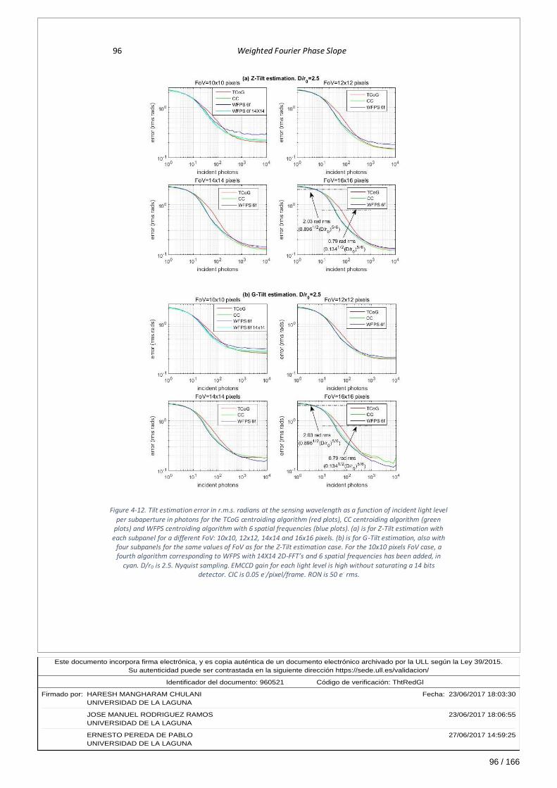
96 / 166
Este documento incorpora firma electrónica, y es copia auténtica de un documento electrónico archivado por la ULL según la Ley 39/2015.Su autenticidad puede ser contrastada en la siguiente dirección https://sede.ull.es/validacion/
Identificador del documento: 960521Código de verificación: ThtRedGl
Firmado por: HARESH MANGHARAM CHULANI Fecha: 23/06/2017 18:03:30UNIVERSIDAD DE LA LAGUNA
JOSE MANUEL RODRIGUEZ RAMOS 23/06/2017 18:06:55UNIVERSIDAD DE LA LAGUNA
ERNESTO PEREDA DE PABLO 27/06/2017 14:59:25UNIVERSIDAD DE LA LAGUNA
96 Weighted Fourier Phase Slope
Figure 4-12. Tilt estimation error in r.m.s. radians at the sensing wavelength as a function of incident light level
per subaperture in photons for the TCoG centroiding algorithm (red plots), CC centroiding algorithm (green plots) and WFPS centroiding algorithm with 6 spatial frequencies (blue plots). (a) is for Z-Tilt estimation with
each subpanel for a different FoV: 10x10, 12x12, 14x14 and 16x16 pixels. (b) is for G-Tilt estimation, also with four subpanels for the same values of FoV as for the Z-Tilt estimation case. For the 10x10 pixels FoV case, a fourth algorithm corresponding to WFPS with 14X14 2D-FFT’s and 6 spatial frequencies has been added, in
cyan. D/r0 is 2.5. Nyquist sampling. EMCCD gain for each light level is high without saturating a 14 bits detector. CIC is 0.05 e-/pixel/frame. RON is 50 e- rms.

97 / 166
Este documento incorpora firma electrónica, y es copia auténtica de un documento electrónico archivado por la ULL según la Ley 39/2015.Su autenticidad puede ser contrastada en la siguiente dirección https://sede.ull.es/validacion/
Identificador del documento: 960521Código de verificación: ThtRedGl
Firmado por: HARESH MANGHARAM CHULANI Fecha: 23/06/2017 18:03:30UNIVERSIDAD DE LA LAGUNA
JOSE MANUEL RODRIGUEZ RAMOS 23/06/2017 18:06:55UNIVERSIDAD DE LA LAGUNA
ERNESTO PEREDA DE PABLO 27/06/2017 14:59:25UNIVERSIDAD DE LA LAGUNA
Chapter 4. Numerical simulations at subpupil level 97
For high light levels of 1000 to 10000 photons per subaperture, detector noises become less
important, and measurement noise is dominated by spot’s deformation due to high order
turbulent phase modes, truncation due to limited FoV, and light shot (intrinsic Poisson) noise.
Note in Figure 4-12 that, for these light levels, the tilt estimation errors are at most in the
order of ~0.3 r.m.s. radians, or one twentieth of wavelength size, for the worst cases, and
hence it can be stated that all the algorithms work fine in these scenarios. However, certain
minor differences can be seen, and it is interesting to reflect on them because it throws light
on the particularities of each algorithm.
For the Z-Tilt estimation in Figure 4-12(a), for the 10x10 pixels case, it can be seen that, for
high light levels, the WFPS algorithm (blue trace) has a tilt estimation error of the order of
~0.3 r.m.s. radians, whereas CC (green trace) and TCoG (red trace) have errors in the order
of ~0.2 r.m.s. radians, slightly higher for the CC algorithm. In this scenario, the dominating
error cause is truncation of the spot due to limited FoV. It was seen in point 4.2 that for a D/r0
ratio of 2.5, a minimum of 12x12 pixels FoV was necessary to adequately cope for the whole
dynamic range of the signal. The reason for the CC and TCoG algorithms’ better behaviour in
this scenario is a powerful tool they have to estimate Z-Tilt over a truncated spot:
thresholding. The Z-Tilt information is in the more symmetric part of the spot around its
maximum, and thresholding is an adequate means to eliminate the low light level asymmetric
part of the spot, including the effect of truncation due to limited FoV. WFPS, on its side, can
deal with spot’s truncation by employing a larger 2D-FFT size than the FoV. A fourth trace in
cyan colour has been added to the figure for the 10x10 FoV case, corresponding to a WFPS
algorithm employing 14x14 2D-FFT’s, and selecting the six lowermost spatial frequencies.
Note that this last trace gets confounded with the green trace of the CC algorithm. This
improvement is explained because of the symmetrizing capacity of the WFPS algorithm over
a spot right in the border of the FoV when a larger 2D-FFT is employed, as illustrated in the
example in point A.5.3, appendix A.
Continuing with the Z-Tilt estimation case, as the FoV gets larger, and for high light levels, the
behaviour of all algorithms is very similar. In this scenario, atmospheric turbulence high order
modes dominate the noise. Thresholding is a good means of selecting the symmetric part of
the spot, as was explained, and so this similarity in their behaviour is not surprising.
For G-Tilt estimation (Figure 4-12-b), high light levels and a FoV of 10x10 pixels, all the
algorithms have a tilt estimation error around ~0.3 r.m.s. radians. The reason is that, in this
case, for G-Tilt estimation, thresholding is not a good tool to employ against spot’s truncation,
because the G-Tilt information is precisely in the asymmetric part of the spot. The only means
to improve this is increasing the FoV and letting this information in, as can be seen in the
following subpanels for FoV’s of 12x12, 14x14 and 16x16 pixels. Something that catches the
attention is that the WFPS outperforms the other two when FoV increases (see the 16x16 FoV
subpanel at light levels from 1000 to 10000 photons). The reason for this is a better capacity
of the WFPS algorithm to reach a compromise between filtering out the detector noise which
is still present and respecting the spot’s asymmetries, whereas CC and TCoG cannot reach
such a compromise by simple thresholding.
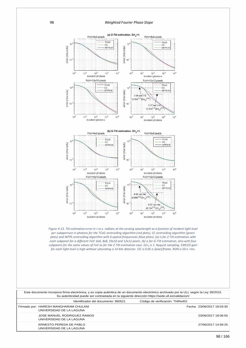
98 / 166
Este documento incorpora firma electrónica, y es copia auténtica de un documento electrónico archivado por la ULL según la Ley 39/2015.Su autenticidad puede ser contrastada en la siguiente dirección https://sede.ull.es/validacion/
Identificador del documento: 960521Código de verificación: ThtRedGl
Firmado por: HARESH MANGHARAM CHULANI Fecha: 23/06/2017 18:03:30UNIVERSIDAD DE LA LAGUNA
JOSE MANUEL RODRIGUEZ RAMOS 23/06/2017 18:06:55UNIVERSIDAD DE LA LAGUNA
ERNESTO PEREDA DE PABLO 27/06/2017 14:59:25UNIVERSIDAD DE LA LAGUNA
98 Weighted Fourier Phase Slope
Figure 4-13. Tilt estimation error in r.m.s. radians at the sensing wavelength as a function of incident light level per subaperture in photons for the TCoG centroiding algorithm (red plots), CC centroiding algorithm (green
plots) and WFPS centroiding algorithm with 6 spatial frequencies (blue plots). (a) is for Z-Tilt estimation with
each subpanel for a different FoV: 6x6, 8x8, 10x10 and 12x12 pixels. (b) is for G-Tilt estimation, also with four subpanels for the same values of FoV as for the Z-Tilt estimation case. D/r0 is 1. Nyquist sampling. EMCCD gain
for each light level is high without saturating a 14 bits detector. CIC is 0.05 e -/pixel/frame. RON is 50 e- rms.

99 / 166
Este documento incorpora firma electrónica, y es copia auténtica de un documento electrónico archivado por la ULL según la Ley 39/2015.Su autenticidad puede ser contrastada en la siguiente dirección https://sede.ull.es/validacion/
Identificador del documento: 960521Código de verificación: ThtRedGl
Firmado por: HARESH MANGHARAM CHULANI Fecha: 23/06/2017 18:03:30UNIVERSIDAD DE LA LAGUNA
JOSE MANUEL RODRIGUEZ RAMOS 23/06/2017 18:06:55UNIVERSIDAD DE LA LAGUNA
ERNESTO PEREDA DE PABLO 27/06/2017 14:59:25UNIVERSIDAD DE LA LAGUNA
Chapter 4. Numerical simulations at subpupil level 99
Straight lines corresponding to 2.03 and 0.79 rms radians have been added to the graph. 2.03
rms radians correspond to the energy in the tip and tilt modes in a turbulence following
Kolmogorov statistics, when D/r0 ratio is 2.5, according to the Noll coefficients derived in Noll,
1976. In the same reference, the remaining turbulent energy when tip and tilt are corrected
can be found in the third Noll coefficient, and gives a value of 0.79 rms radians for the same
D/r0 ratio, being this a kind of fitting error at the subpupil level.
Figure 4-13 shows the results for a repetition of the previous simulation with the same system
parameters values except that the D/r0 ratio value is unity, and FoV’s values are 6x6, 8x8,
10x10 and 12x12 pixels. It is interesting to see that, because the spot is less aberrated by
atmospheric turbulence than in the previous D/r0=2.5 case, all the considerations regarding
spot’s deformation and truncation, though still present, are much ameliorated. For the
smallest FoV values the behaviour of the algorithms is quite indistinguishable, especially for
G-Tilt estimation. When the FoV value increases, an improved behaviour can be seen in the
CC and WFPS algorithms with respect to the TCoG algorithm for light levels between 20 and
200 photons, due to their robustness against detector noises, as was seen in for the D/r0=2.5
case.
4.5. Effect of turbulence strength
Increase in turbulence strength has a twofold effect on tilt estimation in a subpupil of a
SHWFS. First, when sensing the wavefront in an open loop configuration, the tilt dynamic
range will increase, and a larger FoV will be required. A larger FoV implies more detector pixels
and, hence, more measurement noise. Second, high order aberrations will be more
pronounced, the spot will be further away from its diffraction shape and its energy
disseminated among more pixels, all this making tilt estimation noisier.
The purpose of the present point is to show the results of a simulation that assesses the effect
of turbulence strength in subpupil tilt estimation, for two centroinding algorithms: TCoG and
WFPS with 6 spatial frequencies; CC algorithm, as was seen in point 4.4, has a behaviour
almost identical to WFPS, in almost all system configurations simulated. As the turbulence
strength increases, the FoV will be also increased in the simulation, as per shown in Table 4-8.
Two light level regimes are considered for the purpose of FoV selection. When incident light
level is 200 photons or below, the selected FoV is slightly smaller for the TCoG algorithm than
for the WFPS algorithm. When light level is 300 photons or above, the FoV is larger than for
the dimmer light level, and the same for both algorithms. The intention is to be as close as
possible to the optimum field of view determined in point 4.2.1. For the D/r0 ratios not studied
in the mentioned point, FoV values have been approximately inferred from the corresponding
to the studied D/r0 ratios.
As regards the other system configuration parameters, they do not vary with respect to the
previous simulations. Open loop observation is assumed, in a circular subpupil. D/r0 ratio
varies from 0.5, corresponding to a very well sampled pupil, or a very good turbulence
scenario, to 3. Above a ratio of 3, the overall correction that the system can achieve from the
recovered phase modes becomes too low. Sampling of the spot follows the Nyquist criteria,

100 / 166
Este documento incorpora firma electrónica, y es copia auténtica de un documento electrónico archivado por la ULL según la Ley 39/2015.Su autenticidad puede ser contrastada en la siguiente dirección https://sede.ull.es/validacion/
Identificador del documento: 960521Código de verificación: ThtRedGl
Firmado por: HARESH MANGHARAM CHULANI Fecha: 23/06/2017 18:03:30UNIVERSIDAD DE LA LAGUNA
JOSE MANUEL RODRIGUEZ RAMOS 23/06/2017 18:06:55UNIVERSIDAD DE LA LAGUNA
ERNESTO PEREDA DE PABLO 27/06/2017 14:59:25UNIVERSIDAD DE LA LAGUNA
100 Weighted Fourier Phase Slope
that is, FWHM of the spot at diffraction limit is 2 pixels. Simulated QE of the detector is 97%,
and the EMCCD gain is as high as possible without saturating a 14 bits detector. CIC noise is
0.05 e-/pixel/frame, and RON is 50 r.m.s. e-.
Figure 4-14. Tilt estimation error in r.m.s. radians as a function of subpupil diameter to Fried parameter ratio (D/r0) for incident light levels of 30, 50, 100, 200, 300 and 10000 photons and two centroiding algorithms: TCoG and WFPS with 6 spatial frequencies selected. FoV values are as per Table 4-8. (a) is for Z-Tilt estimation. (b) is for G-Tilt estimation. Nyquist sampling. QE is 97%. EMCCD gain for each light level is high without saturating a
14 bits detector. CIC is 0.05 e-/pixel/frame. RON is 50 e- rms.

101 / 166
Este documento incorpora firma electrónica, y es copia auténtica de un documento electrónico archivado por la ULL según la Ley 39/2015.Su autenticidad puede ser contrastada en la siguiente dirección https://sede.ull.es/validacion/
Identificador del documento: 960521Código de verificación: ThtRedGl
Firmado por: HARESH MANGHARAM CHULANI Fecha: 23/06/2017 18:03:30UNIVERSIDAD DE LA LAGUNA
JOSE MANUEL RODRIGUEZ RAMOS 23/06/2017 18:06:55UNIVERSIDAD DE LA LAGUNA
ERNESTO PEREDA DE PABLO 27/06/2017 14:59:25UNIVERSIDAD DE LA LAGUNA
Chapter 4. Numerical simulations at subpupil level 101
Figure 4-14 shows the result of the simulation. Tilt estimation error is plotted versus the D/r0
ratio for the two mentioned algorithms and light levels of 30, 50, 100, 200, 300 and 10000
photons per subaperture. Red traces are for the TCoG algorithm and blue traces are for the
WFPS algorithm. (a) subpanel is for Z-Tilt estimation and (b) is for G-Tilt. All the graphs,
especially the ones for 30, 50 and 100 photons, clearly indicate that WFPS algorithm permits
to operate at worse turbulence strength scenarios for a particular performance assessed by
tilt estimation error. For example, at a 100 photons light regime, performance with the WFPS
algorithm at a particular D/r0 ratio is similar to the performance with the TCoG algorithm at a
0.5 smaller D/ r0 ratio. If, for example, the system requires a maximum tilt estimation error at
subpupil level of 0.4 r.m.s. radians, which is approximately ~λ/15 (at the sensing wavelength),
and the subaperture diameter is 40 cm, for the TCoG algorithm the Fried paramenter r0 should
not go much below 20 cm, whereas for the WFPS algorithm it can go as low as 16 cm, for a
light regime of 100 photons.
4.6. Closed-loop operation simulation
So far, all simulations in this chapter have assumed that the system works in open loop
correction and, so, the atmosphere is sensed in its full dynamic range, without any correction.
In the present point, closed loop system correction is assumed. As explained in point 1.2.1
and illustrated in Figure 1-2, in closed loop operation, the corrective deformable mirror comes
in the optical path before the wavefront sensor, and so, the latter senses a corrected
wavefront. For a SHWFS, this means that the spot corresponding to each subaperture will stay
near the set-point reference when the correction is good. Therefore, at a subpupil level,
closed loop operation can be simulated by attenuating the tip and tilt modes by a correction
factor. In the present point, an attenuation factor of 10 has been employed for all scenarios.
This implies that the assumption is made that the servo correction is independent of such
variables as measurement noise, image size or computational cost. Moreover, system
instabilities are not being taken into account, even when the wavefront measurement is
dominated by noise. These assumptions are justified because the present simulations do not
intend to assess the closed loop behaviour of the system, but just to compare the
performance of several centroiding algorithms when the system geometry has been
adequated to closed loop operation.
Employed FoV (pixels x pixels) for turbulence strength effect assessment
#photons per subaperture
D/r0
0.5 1 1.5 2 2.5 3
200 and below
TCoG 6x6 6x6 8x8 10x10 12x12 14x14
WFPS 6f 8x8 8x8 10x10 12x12 14x14 16x16
300 and above TCoG
12x12 12x12 14x14 14x14 16x16 16x16
WFPS 6f Table 4-8. Employed FoV in pixels by pixels for the assessment of the effect of turbulence strength, the results of
which are illustrated in Figure 4-14.
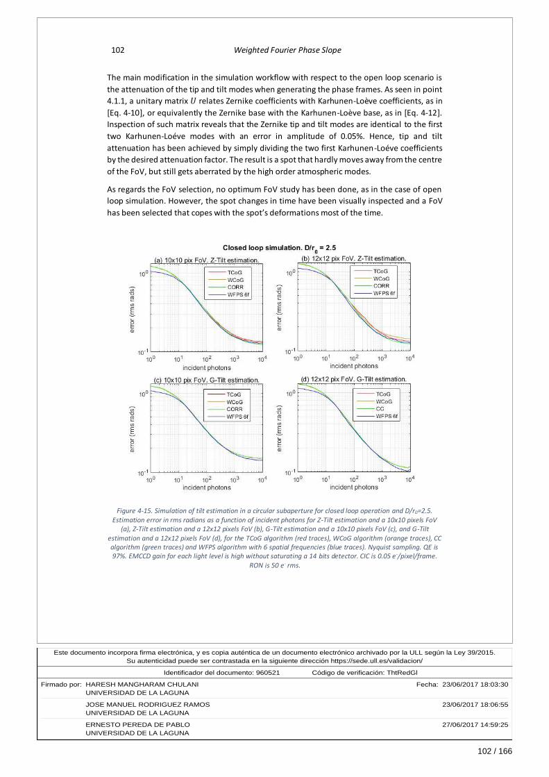
102 / 166
Este documento incorpora firma electrónica, y es copia auténtica de un documento electrónico archivado por la ULL según la Ley 39/2015.Su autenticidad puede ser contrastada en la siguiente dirección https://sede.ull.es/validacion/
Identificador del documento: 960521Código de verificación: ThtRedGl
Firmado por: HARESH MANGHARAM CHULANI Fecha: 23/06/2017 18:03:30UNIVERSIDAD DE LA LAGUNA
JOSE MANUEL RODRIGUEZ RAMOS 23/06/2017 18:06:55UNIVERSIDAD DE LA LAGUNA
ERNESTO PEREDA DE PABLO 27/06/2017 14:59:25UNIVERSIDAD DE LA LAGUNA
102 Weighted Fourier Phase Slope
The main modification in the simulation workflow with respect to the open loop scenario is
the attenuation of the tip and tilt modes when generating the phase frames. As seen in point
4.1.1, a unitary matrix 𝑈 relates Zernike coefficients with Karhunen-Loève coefficients, as in
[Eq. 4-10], or equivalently the Zernike base with the Karhunen-Loève base, as in [Eq. 4-12].
Inspection of such matrix reveals that the Zernike tip and tilt modes are identical to the first
two Karhunen-Loéve modes with an error in amplitude of 0.05%. Hence, tip and tilt
attenuation has been achieved by simply dividing the two first Karhunen-Loéve coefficients
by the desired attenuation factor. The result is a spot that hardly moves away from the centre
of the FoV, but still gets aberrated by the high order atmospheric modes.
As regards the FoV selection, no optimum FoV study has been done, as in the case of open
loop simulation. However, the spot changes in time have been visually inspected and a FoV
has been selected that copes with the spot’s deformations most of the time.
Figure 4-15. Simulation of tilt estimation in a circular subaperture for closed loop operation and D/r0=2.5. Estimation error in rms radians as a function of incident photons for Z-Tilt estimation and a 10x10 pixels FoV
(a), Z-Tilt estimation and a 12x12 pixels FoV (b), G-Tilt estimation and a 10x10 pixels FoV (c), and G-Tilt
estimation and a 12x12 pixels FoV (d), for the TCoG algorithm (red traces), WCoG algorithm (orange traces), CC algorithm (green traces) and WFPS algorithm with 6 spatial frequencies (blue traces). Nyquist sampling. QE is 97%. EMCCD gain for each light level is high without saturating a 14 bits detector. CIC is 0.05 e-/pixel/frame.
RON is 50 e- rms.

103 / 166
Este documento incorpora firma electrónica, y es copia auténtica de un documento electrónico archivado por la ULL según la Ley 39/2015.Su autenticidad puede ser contrastada en la siguiente dirección https://sede.ull.es/validacion/
Identificador del documento: 960521Código de verificación: ThtRedGl
Firmado por: HARESH MANGHARAM CHULANI Fecha: 23/06/2017 18:03:30UNIVERSIDAD DE LA LAGUNA
JOSE MANUEL RODRIGUEZ RAMOS 23/06/2017 18:06:55UNIVERSIDAD DE LA LAGUNA
ERNESTO PEREDA DE PABLO 27/06/2017 14:59:25UNIVERSIDAD DE LA LAGUNA
Chapter 4. Numerical simulations at subpupil level 103
Figure 4-16. Simulation of tilt estimation in a circular subaperture for closed loop operation and D/r0=1.
Estimation error in rms radians as a function of incident photons for Z-Tilt estimation and a 6x6 pixels FoV (a), Z-Tilt estimation and a 8x8 pixels FoV (b), G-Tilt estimation and a 6x6 pixels FoV (c), and G-Tilt estimation and a
8x8 pixels FoV (d), for the TCoG algorithm (red traces), WCoG algorithm (orange traces), CC algorithm (green traces) and WFPS algorithm with 6 spatial frequencies (blue traces). Nyquist sampling. QE is 97%. EMCCD gain
for each light level is high without saturating a 14 bits detector. CIC is 0.05 e -/pixel/frame. RON is 50 e- rms.
Figure 4-15 show the result of tilt estimation error in r.m.s. radians for the sensing wavelength
as a function of incident photons per subaperture, for a closed loop scenario with D/r0=2.5.
Selected FoV’s are 10x10 and 12x12 pixels, and for each FoV both Z-Tilt and G-Tilt have been
estimated, making up a total of four subpanels labelled from (a) to (d). In each case, four
algorithms have been simulated: TCoG (red traces), WCoG (orange traces), CC (green traces)
and WFPS with 6 spatial frequencies (blue traces). WCoG algorithm, which was explained in
point 1.4.1.2, has been added as an algorithm which is appropriate for closed loop operation
when weights are kept fixed in the FoV. Width of the Gaussian weights are optimized by
minimizing the tilt estimation error of the sequence of images under study. Figure 4-16 shows
the same kind of results for a scenario with D/r0=1 and selected FoV’s of 6x6 and 8x8 pixels.
As a general conclusion extracted from these results, there is hardly any difference in
performance between the simulated algorithms for the most common light level regimes,
from 10 to 1000 photons. The reduced number of pixels involved implies a reduced amount
of detector noise, and the simple TCoG is sufficient to get a near optimum performance. As
the spot does not move much from the centre of the FoV, the effect of an evenly distributed

104 / 166
Este documento incorpora firma electrónica, y es copia auténtica de un documento electrónico archivado por la ULL según la Ley 39/2015.Su autenticidad puede ser contrastada en la siguiente dirección https://sede.ull.es/validacion/
Identificador del documento: 960521Código de verificación: ThtRedGl
Firmado por: HARESH MANGHARAM CHULANI Fecha: 23/06/2017 18:03:30UNIVERSIDAD DE LA LAGUNA
JOSE MANUEL RODRIGUEZ RAMOS 23/06/2017 18:06:55UNIVERSIDAD DE LA LAGUNA
ERNESTO PEREDA DE PABLO 27/06/2017 14:59:25UNIVERSIDAD DE LA LAGUNA
104 Weighted Fourier Phase Slope
noise across the FoV is small, and the WFPS algorithm tends to give high weight values to the
zero spatial frequency, thus getting near a CoG algorithm.
On the other hand, the selected FoV’s are small enough and sufficient, and this can be seen
in the estimation error for high light level conditions: for Z-Tilt estimation there is not much
change with increased FoV, whereas for G-Tilt estimation there is a slight, small improvement
when FoV increases, as more of the spot’s “skirt” is captured.
4.7. Square subaperture
Manufacturers offer both circular and square shaped microlenses arrays. So far, the
simulations in this chapter have assumed a circular shaped subaperture. In this point, results
are shown of an assessment of the applicability of the WFPS algorithm to the case of a square
shaped microlens.
Zernike functions are in principle defined for a circular aperture. The simulation method of
Kolmogorov phase frames as explained in point 4.1.1 has the Zernike coefficients’ covariance
matrix for Kolmogorov turbulence as a starting point, and this assumes a circular aperture in
the system. In order to simulate Kolmogorov turbulence as seen from a square subaperture,
first a turbulent phase in a circular subaperture has been simulated, and then a square shaped
piece of that phase has been selected, as shown in Figure 4-17.
Figure 4-17. The largest square shaped portion of the Kolmogorov circular phase is extracted to simulate a square subaperture.
From the square shaped phase thus obtained, an image in the focal plane of the microlens is
derived as explained in point 4.1.2. All the exposed formulation in the mentioned point is valid
for a square subaperture, taking into account that D is the side of the square and that Np is
the number of pixels of phase corresponding to the length of D.
Another necessary issue to consider when the aperture is square in shape is the definition of
Zernike tilt, which is in principle dependent upon the Zernike tip and tilt modes defined in a
circular aperture. The equivalent modes for a square subaperture are a horizontally inclined
plane and a vertically inclined plane over the square, which we may call 𝑍2𝑆𝑄𝑅 and 𝑍3
𝑆𝑄𝑅 ,
respectively. If 𝜙𝑆𝑄𝑅 is the square shaped phase extracted from the circular shaped phase 𝜙,
Kolmogorov phase
is simulated in a
circular aperture
The largest square
shaped portion of
the phase is
extracted
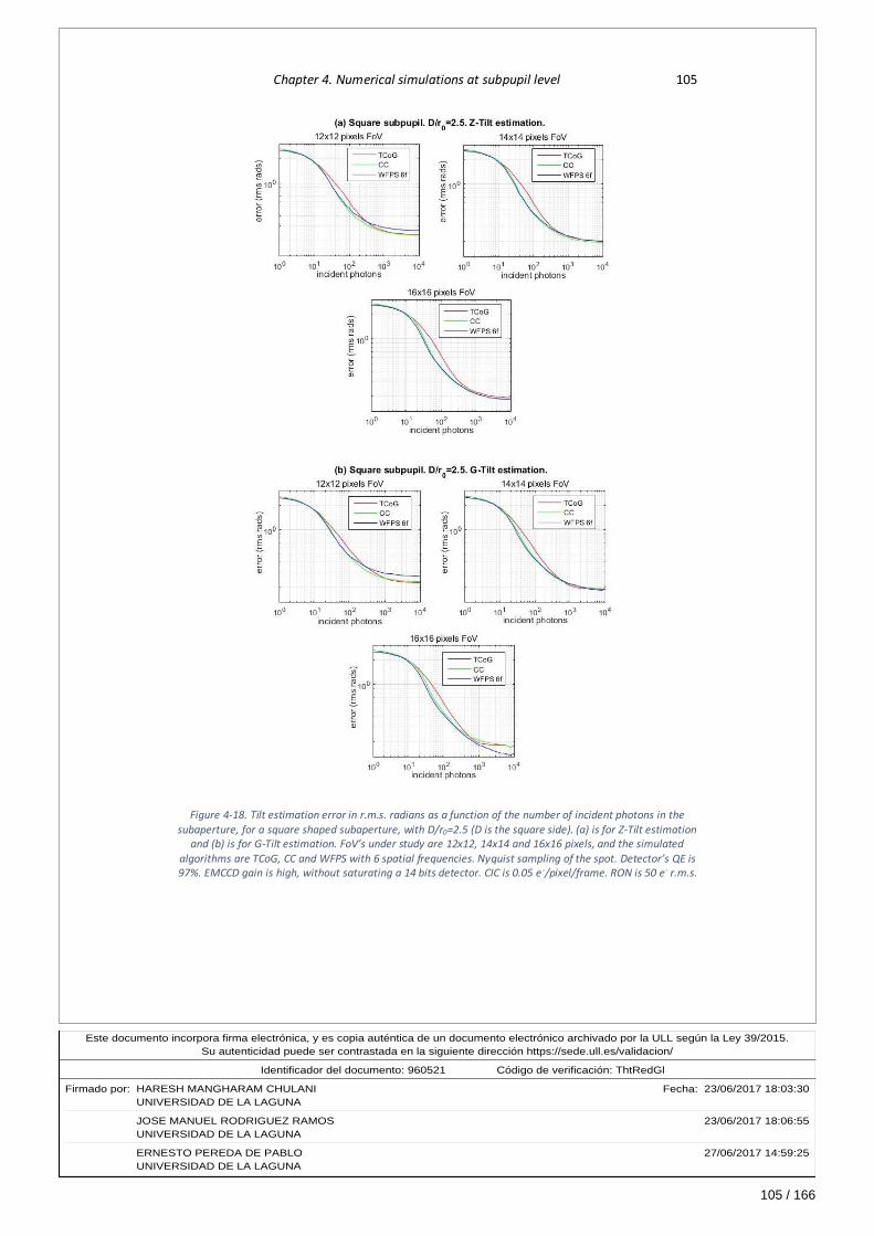
105 / 166
Este documento incorpora firma electrónica, y es copia auténtica de un documento electrónico archivado por la ULL según la Ley 39/2015.Su autenticidad puede ser contrastada en la siguiente dirección https://sede.ull.es/validacion/
Identificador del documento: 960521Código de verificación: ThtRedGl
Firmado por: HARESH MANGHARAM CHULANI Fecha: 23/06/2017 18:03:30UNIVERSIDAD DE LA LAGUNA
JOSE MANUEL RODRIGUEZ RAMOS 23/06/2017 18:06:55UNIVERSIDAD DE LA LAGUNA
ERNESTO PEREDA DE PABLO 27/06/2017 14:59:25UNIVERSIDAD DE LA LAGUNA
Chapter 4. Numerical simulations at subpupil level 105
Figure 4-18. Tilt estimation error in r.m.s. radians as a function of the number of incident photons in the subaperture, for a square shaped subaperture, with D/r0=2.5 (D is the square side). (a) is for Z-Tilt estimation
and (b) is for G-Tilt estimation. FoV’s under study are 12x12, 14x14 and 16x16 pixels, and the simulated
algorithms are TCoG, CC and WFPS with 6 spatial frequencies. Nyquist sampling of the spot. Detector’s QE is 97%. EMCCD gain is high, without saturating a 14 bits detector. CIC is 0.05 e -/pixel/frame. RON is 50 e- r.m.s.
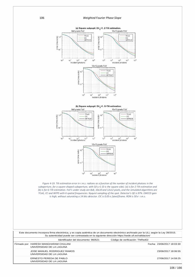
106 / 166
Este documento incorpora firma electrónica, y es copia auténtica de un documento electrónico archivado por la ULL según la Ley 39/2015.Su autenticidad puede ser contrastada en la siguiente dirección https://sede.ull.es/validacion/
Identificador del documento: 960521Código de verificación: ThtRedGl
Firmado por: HARESH MANGHARAM CHULANI Fecha: 23/06/2017 18:03:30UNIVERSIDAD DE LA LAGUNA
JOSE MANUEL RODRIGUEZ RAMOS 23/06/2017 18:06:55UNIVERSIDAD DE LA LAGUNA
ERNESTO PEREDA DE PABLO 27/06/2017 14:59:25UNIVERSIDAD DE LA LAGUNA
106 Weighted Fourier Phase Slope
Figure 4-19. Tilt estimation error in r.m.s. radians as a function of the number of incident photons in the subaperture, for a square shaped subaperture, with D/r0=1 (D is the square side). (a) is for Z-Tilt estimation and (b) is for G-Tilt estimation. FoV’s under study are 8x8, 10x10 and 12x12 pixels, and the simulated algorithms are
TCoG, CC and WFPS with 6 spatial frequencies. Nyquist sampling of the spot. Detector’s QE is 97%. EMCCD gain is high, without saturating a 14 bits detector. CIC is 0.05 e -/pixel/frame. RON is 50 e- r.m.s.
107 / 166
Este documento incorpora firma electrónica, y es copia auténtica de un documento electrónico archivado por la ULL según la Ley 39/2015.Su autenticidad puede ser contrastada en la siguiente dirección https://sede.ull.es/validacion/
Identificador del documento: 960521Código de verificación: ThtRedGl
Firmado por: HARESH MANGHARAM CHULANI Fecha: 23/06/2017 18:03:30UNIVERSIDAD DE LA LAGUNA
JOSE MANUEL RODRIGUEZ RAMOS 23/06/2017 18:06:55UNIVERSIDAD DE LA LAGUNA
ERNESTO PEREDA DE PABLO 27/06/2017 14:59:25UNIVERSIDAD DE LA LAGUNA
Chapter 4. Numerical simulations at subpupil level 107
then the coefficients which quantify the amount of tip and tilt in the square aperture can be
calculated by orthogonal projection of 𝜙𝑆𝑄𝑅 over 𝑍2𝑆𝑄𝑅 and 𝑍3
𝑆𝑄𝑅 , as in [Eq. 4-26]:
𝑐2𝑆𝑄𝑅
=∬𝜙𝑆𝑄𝑅 ⋅ 𝑍2
𝑆𝑄𝑅𝑑𝑥𝑑𝑦
∬𝑍2𝑆𝑄𝑅
⋅ 𝑍2𝑆𝑄𝑅𝑑𝑥𝑑𝑦
𝑐3𝑆𝑄𝑅
=∬𝜙𝑆𝑄𝑅 ⋅ 𝑍3
𝑆𝑄𝑅𝑑𝑥𝑑𝑦
∬𝑍3𝑆𝑄𝑅
⋅ 𝑍3𝑆𝑄𝑅𝑑𝑥𝑑𝑦
[Eq. 4-26]
𝑐2𝑆𝑄𝑅
and 𝑐3𝑆𝑄𝑅
would be the coefficients of an expansion of 𝜙𝑆𝑄𝑅over a set of orthogonal
functions in the square subaperture, with tip and tilt represented by 𝑍2𝑆𝑄𝑅 and 𝑍3
𝑆𝑄𝑅 .
As for the r.m.s. tip and tilt values related to the 𝑐2𝑆𝑄𝑅
and 𝑐3𝑆𝑄𝑅
coefficients, these can be
calculated as:
Δϕ𝑟𝑚𝑠𝑆𝑄𝑅|ℎ𝑜𝑟𝑖𝑧
= 𝑐2𝑆𝑄𝑅
[1
𝑆𝑆𝑄𝑅∬𝑍2
𝑆𝑄𝑅⋅ 𝑍2
𝑆𝑄𝑅𝑑𝑥𝑑𝑦]
1/2
Δϕ𝑟𝑚𝑠𝑆𝑄𝑅|
𝑣𝑒𝑟𝑡= 𝑐3
𝑆𝑄𝑅 [1
𝑆𝑆𝑄𝑅∬𝑍3
𝑆𝑄𝑅 ⋅ 𝑍3𝑆𝑄𝑅𝑑𝑥𝑑𝑦]
1/2
[Eq. 4-27]
with 𝑆𝑆𝑄𝑅 being the area of the square subaperture. These are the true tilt r.m.s. values to be
compared with the r.m.s. recovered tilt values from the image’s displacement and obtained
from [Eq. 4-25].
When comparing the images at focal plane corresponding to a square subpupil and a circular
subpupil with the diameter length equal to the square subpupil’s side, the most evident
difference is that a cross shaped spot comes out of the square subpupil, whereas the spot for
the circular subaperture is circularly symmetric. Second, more light passes through the square
subaperture, approximately a 25% more. And third, more turbulence is seen through the
square subaperture, leading to a more aberrated spot.
Figure 4-18 shows the results of the tilt recovery error in r.m.s. radians as a function of
incident photons per subaperture for image sequences obtained from a square shaped
subpupil. The ratio of subaperture side to Fried parameter is D/r0=2.5. Open loop sensing is
assumed. Spot’s sampling follows Nyquist criterion and, so, FWHM at diffraction limit is 2
pixels wide. FoV’s under study are 12x12, 14x14, and 16x16 pixels. The applied centroiding
algorithms are TCoG (red traces), CC (green traces) and WFPS with six spatial frequencies
(blue traces). Panel (a) is for Z-Tilt estimation and panel (b) is for G-Tilt estimation. The
detector’s gain and noise parameters are as for the rest of simulations in this chapter.
A very similar behaviour of all the algorithms to the circular subpupil case (section 4.4) can be
seen. For low to moderate light levels, detector noise dominates and the spot’s shape is
unimportant. Errors are somewhat higher than for the circular subpupil case for the three
algorithms at a particular light level, most probably because of the increase in higher order
turbulent aberrations, but this gets compensated for the most common light levels by the fact
that more light gets through the square subpupil. Tilt estimation improvement of CC and

108 / 166
Este documento incorpora firma electrónica, y es copia auténtica de un documento electrónico archivado por la ULL según la Ley 39/2015.Su autenticidad puede ser contrastada en la siguiente dirección https://sede.ull.es/validacion/
Identificador del documento: 960521Código de verificación: ThtRedGl
Firmado por: HARESH MANGHARAM CHULANI Fecha: 23/06/2017 18:03:30UNIVERSIDAD DE LA LAGUNA
JOSE MANUEL RODRIGUEZ RAMOS 23/06/2017 18:06:55UNIVERSIDAD DE LA LAGUNA
ERNESTO PEREDA DE PABLO 27/06/2017 14:59:25UNIVERSIDAD DE LA LAGUNA
108 Weighted Fourier Phase Slope
WFPS algorithms over the TCoG algorithm for light levels from 20 to 200 incident photons is
very similar to the circular subpupil case. For example, for the 16x16 pixels FoV case and for
50 incident photons, CC and WFPS commit an error of ~0.65 rms radians when estimating Z-
Tilt, which is in the order of one tenth of the sensing wavelength, whereas TCoG’s error is in
the order of ~1 rms radian for the same light level, or the same error at double the light level,
or 100 incident photons. Error estimation improvement at 50 photons is, therefore, of ~35%.
Very similar figures can be seen for the G-Tilt estimation.
MAP weights for the WFPS algorithm are also very similar to the circular subpupil case for low
to moderate light levels, thus indicating that detector noise dominates. For high light levels
above 500 photons, weights are more concentrated at zero spatial frequency than for the
circular subpupil case, probably because of the increased spot’s aberration. At these light
levels, the three algorithms have a similar tilt estimation error. For the case of 16x16 pixels
FoV and G-Tilt estimation, WFPS outperforms the other two, because it can better take into
account the assymetries of the spot in the presence of noise, same as happened in the circular
subpupil case.
Figure 4-19 shows the results of an identical simulation when reducing the D/r0 ratio to unity
and the FoV’s to 8x8, 10x10 and 12x12 pixels. As it was seen for the circular subpupil case,
the three algorithm’s performances tend to get closer to each other, especially for the lowest
FoV case of 8x8 pixels. For the larger FoV’s and light levels of 20 to 200 incident photons, an
improvement of tilt estimation for CC and WFPS algorithms as compared to the TCoG
algorithm can be seen, which can reach a ~40% for 12x12 pixels FoV and Z-Tilt estimation at
50 incident photons. At high light levels, performance of the three algorithms is again very
similar to each other and to the circular subpupil case.
4.8. Conclusions of this chapter
The Weighted Fourier Phase Slope algorithm has been characterized and compared to other
commonly used algorithms such as TCoG and CC for open loop wavefront sensing and also to
WCoG for closed loop wavefront sensing.
It has been seen that the selection of the lowermost six spatial frequencies in the WFPS
algorithm is a good compromise between tilt estimation performance and computational
cost, thus leading to a hardware speed requirement of one order of magnitude less than for
the CC algorithm implemented in the Fourier domain (this last issue was seen in section 3.3,
point 3.3.5). Further increasing the number of spatial frequencies leads to only a slight
improvement in tilt estimation performance.
The required linearity when observing in open loop configuration is equally good for WFPS,
CC and TCoG algorithms when the selected FoV spans the tilt’s full dynamic range. When the
FoV is shortened, TCoG and CC increase their threshold values in order to overcome the spot’s
truncation effect over the tilt estimation. WFPS algorithm does not have this advantage,
unless a thresholded variation of it is implemented. However, it can overcome the spot’s
truncation and reach a similar tilt estimation performance than the other two algorithms by
employing larger 2D-FFT’s than the size of the FoV.

109 / 166
Este documento incorpora firma electrónica, y es copia auténtica de un documento electrónico archivado por la ULL según la Ley 39/2015.Su autenticidad puede ser contrastada en la siguiente dirección https://sede.ull.es/validacion/
Identificador del documento: 960521Código de verificación: ThtRedGl
Firmado por: HARESH MANGHARAM CHULANI Fecha: 23/06/2017 18:03:30UNIVERSIDAD DE LA LAGUNA
JOSE MANUEL RODRIGUEZ RAMOS 23/06/2017 18:06:55UNIVERSIDAD DE LA LAGUNA
ERNESTO PEREDA DE PABLO 27/06/2017 14:59:25UNIVERSIDAD DE LA LAGUNA
Chapter 4. Numerical simulations at subpupil level 109
As regards sensitivity in low to moderate light level conditions, CC and WFPS algorithms, while
being very similar to each other, outperform the TCoG algorithm for light levels between 20
and 200 photons for typical values of detector’s gain and CIC and RON noises. Simple
thresholding finds itself to be limited in the simultaneous presence of turbulence high order
aberrations and non-Gaussian type of detector’s noise, such as amplified CIC noise, for the
mentioned light levels. By prefiltering with a correlation such as in the CC algorithm or by
smoothing the phase in the Fourier domain such as in the WFPS algorithm, more robust
centroiding algorithms are achieved in the presence of the mentioned measurement noises.
As the selected or required FoV is increased, this tilt estimation performance difference
between the CC and WFPS algorithms on one side and the TCoG algorithm on the other side
become increasingly evident, as more FoV means more detector pixels and, hence, noise. In
this respect, both CC and WFPS algorithms, at the mentioned light levels, prefer to work with
larger FoV’s than the TCoG algorithm, and are able to cope with worse turbulence scenarios,
maintaining tilt estimation performance.
For high light levels, the three algorithms perform equally as tilt estimation error is concerned.
An exception is the case of large FoV’s and G-Tilt estimation, where the assymetries of the
spot, contained in its low light level portion, are required to be taken into account, in the
presence of noise. Here, the WFPS outperforms the CC and TCoG algorithms, because its
mechanism to supress noise does not use thresholding the image at any moment.
In closed loop wavefront sensing, the required FoV is rather small as the spot is kept fixed at
the reference set-point. The amount of noise in this scenario is therefore small, and the four
studied algorithms (WCoG was added) perform in a very similar manner as regards tilt
estimation.
Finally, an evaluation of the performance of TCoG, CC and WFPS algorithms for open loop
sensing through a square shaped subaperture was made, showing a very similar behaviour as
seen in the circular shaped subaperture.

110 / 166
Este documento incorpora firma electrónica, y es copia auténtica de un documento electrónico archivado por la ULL según la Ley 39/2015.Su autenticidad puede ser contrastada en la siguiente dirección https://sede.ull.es/validacion/
Identificador del documento: 960521Código de verificación: ThtRedGl
Firmado por: HARESH MANGHARAM CHULANI Fecha: 23/06/2017 18:03:30UNIVERSIDAD DE LA LAGUNA
JOSE MANUEL RODRIGUEZ RAMOS 23/06/2017 18:06:55UNIVERSIDAD DE LA LAGUNA
ERNESTO PEREDA DE PABLO 27/06/2017 14:59:25UNIVERSIDAD DE LA LAGUNA
111 / 166
Este documento incorpora firma electrónica, y es copia auténtica de un documento electrónico archivado por la ULL según la Ley 39/2015.Su autenticidad puede ser contrastada en la siguiente dirección https://sede.ull.es/validacion/
Identificador del documento: 960521Código de verificación: ThtRedGl
Firmado por: HARESH MANGHARAM CHULANI Fecha: 23/06/2017 18:03:30UNIVERSIDAD DE LA LAGUNA
JOSE MANUEL RODRIGUEZ RAMOS 23/06/2017 18:06:55UNIVERSIDAD DE LA LAGUNA
ERNESTO PEREDA DE PABLO 27/06/2017 14:59:25UNIVERSIDAD DE LA LAGUNA
Chapter 5. Numerical simulations at an entire pupil level
There are two main sources of measurement error in a Shack-Hartmann Wavefront Sensor,
as it was explained in point 1.2.2.2. First, tilt estimation is affected by measurement noise in
each subpupil, due to the detector’s noises, pixelation, limited FoV and turbulence high order
aberrations. This is the measurement error at the subpupil level and was the object of study
in the previous chapter. Second, a limited number of subpupils implies a limited number of
phase modes recovered, and a consequent fitting error in the estimated phase. This second
source of error works at the entire pupil level, and becomes the dominant measurement error
when tilt estimation at the subpupil level is good. The purpose of the present chapter is to
assess the effect of varying the centroiding algorithm at the subpupil level on the globa l
performance of the SHWFS at the entire pupil level, thus including the fitting error in the
simulation.
The selected tool for this purpose is the Object Oriented Matlab toolbox for Adaptive Optics
(OOMAO, Conan and Correia, 2014). Results are presented as Strehl Ratio (SR) or Encircled
Energy (EE) of the system PSF as a function of star magnitude, for a particular system
configuration and centroiding algorithm, after compensation with the estimated phase at the
entire sensor pupil.
5.1. The Object Oriented Matlab Adaptive Optics toolbox
The OOMAO toolbox is a freely available11 extension of the Matlab™ language, consisting of
a library of Matlab classes oriented towards the numerical modelling of AO systems. Figure
5-1 shows the OOMAO class diagram with the objects disposed as in a closed-loop controlled
system. It has been taken from Conan and Correia, 2014, and shows a complete set of classes
corresponding to an advanced stage of development of the tool. The OA system is created by
selecting and instantiating objects from the available classes, initializing and configuring
them, and assembling them throughout an optical path. The main classes used during a
simulation are:
11 It is downloadable at https://github.com/rconan/OOMAO, as of May, 2017.

112 / 166
Este documento incorpora firma electrónica, y es copia auténtica de un documento electrónico archivado por la ULL según la Ley 39/2015.Su autenticidad puede ser contrastada en la siguiente dirección https://sede.ull.es/validacion/
Identificador del documento: 960521Código de verificación: ThtRedGl
Firmado por: HARESH MANGHARAM CHULANI Fecha: 23/06/2017 18:03:30UNIVERSIDAD DE LA LAGUNA
JOSE MANUEL RODRIGUEZ RAMOS 23/06/2017 18:06:55UNIVERSIDAD DE LA LAGUNA
ERNESTO PEREDA DE PABLO 27/06/2017 14:59:25UNIVERSIDAD DE LA LAGUNA
112 Weighted Fourier Phase Slope
Figure 5-1. OOMAO class diagram, from Conan and Correia, 2014.
source: It can be a single source or an asterism, and a NGS or a LGS. It inherits from
the stochasticWave class the properties of amplitude and phase of an optical wave,
which is propagated through the optical system with the use of the overloaded Matlab
operators .× and ×.
telescope: It contains properties such as the aperture size, central obscuration size,
and spatial and temporal resolution of the system. It is a child of the telescopeAbstract
class, which embeds an atmosphere class instance in order to create the complete
optical system which precedes the AO sensing and corrective components.
atmosphere: The atmospheric phase aberration as a function of time is created in this
class. It embeds one or more turbulenceLayer instances, each with a user defined
height and wind speed and direction.
deformableMirror: The compensation of the atmospheric phase is implemented here.
This object has not been used in the present work. A zernike object has been used
instead in order to subtract a user defined number of Zernike modes from the
propagating wave.
shackHartmann: This class implements the Shack-Hartmann wavefront sensor. Its
properties are related to the phase recovery at each subpupil and at the whole pupil
as well. For example, the selected centroiding algorithm and the values of its
associated parameters such as the TCoG threshold are found in this class, as well as
matrixes that relate phase gradients in the subpupils with phase values in the
subpupils’ corners for a Fried geometry sensor. Since a SHWFS is composed basically

113 / 166
Este documento incorpora firma electrónica, y es copia auténtica de un documento electrónico archivado por la ULL según la Ley 39/2015.Su autenticidad puede ser contrastada en la siguiente dirección https://sede.ull.es/validacion/
Identificador del documento: 960521Código de verificación: ThtRedGl
Firmado por: HARESH MANGHARAM CHULANI Fecha: 23/06/2017 18:03:30UNIVERSIDAD DE LA LAGUNA
JOSE MANUEL RODRIGUEZ RAMOS 23/06/2017 18:06:55UNIVERSIDAD DE LA LAGUNA
ERNESTO PEREDA DE PABLO 27/06/2017 14:59:25UNIVERSIDAD DE LA LAGUNA
Chapter 5. Numerical simulations at an entire pupil level 113
of a lenslet array and a detector, two classes can be found embedded in the
shackHartmann class:
. lensletArray: Properties such as the number of lenslets, number of detector
pixels per lenslet and percentage of light as a criterion to include the subpupils
in the borders, define the objects in this class. Lenslets are square shaped. By
default, the images at the detector are Nyquist sampled, i. e., the FWHM is 2
pixels wide. This can be changed to any desired width by the nyquistSampling
property in this class.
. detector: The main task of this class is to add photonic noise to the light, add a
background light, apply a quantum efficiency and add the readout noise.
imager: This class implements the generation of the final turbulence compensated PSF
as seen by the science detector. It is actually a child of the detector class, and also
embeds an instantation of the lensletArray class to generate a 1 x 1 lenslet array. It
contains properties that allow to define the starting and ending times of light
integration, as well as methods that calculate the Strehl Ratio and Encircled Energy12
over the PSF.
This tool was selected for the whole SHWFS simulation without dedicating much effort to
investigating, comparing and selecting among other tools, mainly because its free cost and
the possibility of reusing Matlab code that was programmed for the simulations at the
subpupil level. Very strong points that could be observed in its design characteristics are its
modularity due to the object-oriented programming, a vectorised code in line with Matlab’s
good programming practice, and Matlab’s parallel computing capabilities usage. The only
weak point to mention is the lack of detailed code documentation, probably because it is a
tool under development yet.
5.1.1. Features added to the OOMAO in the context of the present work
Some features were added to the shackHartmann and its embedded classes lensletArray and
detector, necessary to achieve the desired simulation results. These have been the following:
The possibility of defining a circular subpupil array has been added to the lensletArray
class. The public properties subpupilShape and circularSubpupilRadius have been
added, that allow to select between a square shaped and a circular shaped subpupil,
and define a radius size in pixels for the circular shaped case. A private property called
circularSubpupilMask is used as a mask in the Fraunhoffer image generation at the
propagateThrough method. It is calculated in the setCircularSubpupilMask method,
which is called when the number of pixels per lenslet is defined.
No significant differences were found in the simulation results between circular and
square shaped subpupils, and so the results for circular subpupils will not be shown.
The gain and noise model of an EMCCD camera, as explained in point 4.1.3, has been
added to the detector class through the properties emccdGain and CICNoise. The CIC
12 The Encircled Energy calculation was not implemented at the time the author downloaded the toolbox.

114 / 166
Este documento incorpora firma electrónica, y es copia auténtica de un documento electrónico archivado por la ULL según la Ley 39/2015.Su autenticidad puede ser contrastada en la siguiente dirección https://sede.ull.es/validacion/
Identificador del documento: 960521Código de verificación: ThtRedGl
Firmado por: HARESH MANGHARAM CHULANI Fecha: 23/06/2017 18:03:30UNIVERSIDAD DE LA LAGUNA
JOSE MANUEL RODRIGUEZ RAMOS 23/06/2017 18:06:55UNIVERSIDAD DE LA LAGUNA
ERNESTO PEREDA DE PABLO 27/06/2017 14:59:25UNIVERSIDAD DE LA LAGUNA
114 Weighted Fourier Phase Slope
noise is like a background light with Poisson distribution; it is not affected by the
quantum efficiency, and it is amplified by the EMCCD gain. The EMCCD gain is
implemented through a gamma distribution, as expressed in equation [Eq. 4-20]. Both
items are applied to the image before adding readout noise. In the final offset
subtraction, the mean value of background light, affected by the quantum efficiency
and the EMCCD gain, is subtracted; and the mean CIC noise affected only by the
EMCCD gain is subtracted as well.
The correlation centroiding algorithm has been implemented in the shackHartmann
class. The correlation reference is the diffraction limited image, and is set with the
setCorrelationReference method, which should be called after propagating a planar
wavefront to the SHWFS. The correlation is executed in the Fourier domain, in the
dataProcessing method, where the rest of centroiding algorithms are to be found. A
thresholding can be applied to the correlation figure, through the
correlationThreshold public property, and finally a centre of gravity is applied to the
thresholded correlation figure.
The Weighted Fourier Phase Slope algorithm has been implemented in the
shackHartmann class, at the dataProcessing method. Public properties wfpsWeightsX
and wfpsWeightsY have been included to contain the Bayesian weights at the working
spatial frequencies for the horizontal and vertical centroids calculation, respectively.
An encircled energy computation function has been implemented, where the input
parameters are the PSF, wavelength, pupil diameter, Nyquist sampling factor, total
amount of light at the pupil and a vector of circle diameters in arcsecs, and the output
is the EE as a function of the specified circle diameters.
Figure 5-2 shows three samples of the SHWFS detector’s images created with the OOMAO for
a 20 x 20 square subpupils configuration in a 4.2 m. circular aperture with a central
obscuration of an 8.4% of the aperture’s surface and Nyquist sampling. This will be the
working configuration throughout the simulations presented in this chapter. The first panel,
labelled (a), is for the case of a planar wavefront, a FoV of 10 x 10 pixels, which for a source
wavelength of 550 nm. is a ~2.7” FoV, a very brilliant star of zero magnitude and no noise
sources. In the second panel, labelled (b), the star magnitude is 11. For the default optical
throughput of unity, this means ~31.5 incident photons per subpupil at a system frequency
of 500 Hz. Atmospheric turbulence has been added, with a Fried parameter of 21 cm, which
is equal to the subpupil side size. Poisson photon noise has been enabled; a quantum
efficiency of 97% and an EMCCD gain of 1000 have been applied; and a CIC noise of 0.05 e -
/pixel/frame and a RON noise of 50 rms e- have been added. RON noise is not actually visible
in the figure. The spurious visible noise corresponds to the CIC noise which, when amplified
by the EM register, reaches habitual pixel peak values in the order of ~3000 – 5000 digital
counts for the default detector sensitivity of 1 e-/ADU, thus becoming noticeable against the
spots’ peak values of ~5000 – 10000 digital counts. In the third panel, labelled (c), the FoV
has been increased to 14 x 14 pixels, corresponding to a ~3.8” FoV, in order to cope with the
increase in turbulence strength corresponding to a Fried parameter of 8.4 cm, 2.5 times
smaller than the square subpupil’s side size. The spots are visibly more diffused and the image
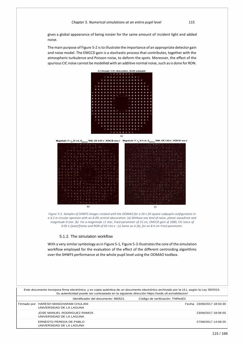
115 / 166
Este documento incorpora firma electrónica, y es copia auténtica de un documento electrónico archivado por la ULL según la Ley 39/2015.Su autenticidad puede ser contrastada en la siguiente dirección https://sede.ull.es/validacion/
Identificador del documento: 960521Código de verificación: ThtRedGl
Firmado por: HARESH MANGHARAM CHULANI Fecha: 23/06/2017 18:03:30UNIVERSIDAD DE LA LAGUNA
JOSE MANUEL RODRIGUEZ RAMOS 23/06/2017 18:06:55UNIVERSIDAD DE LA LAGUNA
ERNESTO PEREDA DE PABLO 27/06/2017 14:59:25UNIVERSIDAD DE LA LAGUNA
Chapter 5. Numerical simulations at an entire pupil level 115
gives a global appearance of being noisier for the same amount of incident light and added
noise.
The main purpose of Figure 5-2 is to illustrate the importance of an appropriate detector gain
and noise model. The EMCCD gain is a stochastic process that contributes, together with the
atmospheric turbulence and Poisson noise, to deform the spots. Moreover, the effect of the
spurious CIC noise cannot be modelled with an additive normal noise, such as is done for RON.
Figure 5-2. Samples of SHWFS images created with the OOMAO for a 20 x 20 square subpupils configuration in a 4.2 m circular aperture with an 8.4% central obscuration. (a) Without any kind of noise, planar wavefront and
magnitude 0 star. (b) For a magnitude 11 star, Fried parameter of 21 cm, EMCCD gain of 1000, CIC noise of 0.05 e-/pixel/frame and RON of 50 rms e-. (c) Same as in (b), for an 8.4 cm Fried parameter.
5.1.2. The simulation workflow
With a very similar symbology as in Figure 5-1, Figure 5-3 illustrates the core of the simulation
workflow employed for the evaluation of the effect of the different centroiding algorithms
over the SHWFS performance at the whole pupil level using the OOMAO toolbox.

116 / 166
Este documento incorpora firma electrónica, y es copia auténtica de un documento electrónico archivado por la ULL según la Ley 39/2015.Su autenticidad puede ser contrastada en la siguiente dirección https://sede.ull.es/validacion/
Identificador del documento: 960521Código de verificación: ThtRedGl
Firmado por: HARESH MANGHARAM CHULANI Fecha: 23/06/2017 18:03:30UNIVERSIDAD DE LA LAGUNA
JOSE MANUEL RODRIGUEZ RAMOS 23/06/2017 18:06:55UNIVERSIDAD DE LA LAGUNA
ERNESTO PEREDA DE PABLO 27/06/2017 14:59:25UNIVERSIDAD DE LA LAGUNA
116 Weighted Fourier Phase Slope
There are two optical paths that share a telescope instance with a 4.2 m. pupil diameter size
and an 8.4% of central obscuration. The telescope instance embeds an atmosphere instance,
which is initialized and configured following a model used in several examples included in the
toolbox: a three-layer model with 0, 5 and 12 km. altitude and fractional r0’s of 0.5, 0.3 and
0.2, respectively; wind speeds are 10, 5 and 20 m/s, and wind directions are 0, π/2 and π. The
system frequency has been set to 500 Hz.
Each optical path has its own source. The one labelled ngs represents the Natural Guide Start
and its light ends up in the shackHartmann object. The second one, labelled science,
represents the scientific object of interest and its light ends up in the imager object through
a zernike object. Both light sources are set to the default wavelength of 550 nm, and therefore
the sensing system performance evaluation is made at the WFS sensing wavelength.
The SHWFS observes the full dynamic range of the atmosphere, as in an open loop
configuration. The shackHartmann object is configured to have a matrix of 20 x 20 square
shaped lenslets, and only the subpupils with a minimum of 85% of light with respect to the
most illuminated one are considered for the phase recovery computation. Sampling of the
spots follows the Nyquist criterion. The number of detector pixels per lenslet has been set to
10 x 10 for the case of a 21 cm r0, making up a ~2.7” FoV, and 14 x 14 for the case of an 8.4
cm r0, making up a ~3.8” FoV. As regards the detector model, a QE of 97% has been applied;
since star magnitudes under study are over 7.5, an EMCCD gain value of 1000 has been
applied, unless otherwise stated; CIC noise has been set to 0.05 e-/pixel/frame, and RON to
50 rms e-. The sensitivity of the detector is the default 1 e-/ADU. It is through the
shackHartmann properties that the centroiding algorithm is selected: Thresholded Centre of
Gravity, Correlation or Weighted Fourier Phase Slope.
Figure 5-3. Core of the simulation workflow programmed in the OOMAO for the assessment of the effect of the centroiding algorithms at a pupil level.
At the other optical path, an imager object receives a compensated wavefront. The corrector
element is a zernike object that receives the corrective Zernike coefficient values from the
shackHartmann instance. This correction is applied with the same spatial resolution in the
pupil as the one defined in the telescope and shackHartmann objects, i.e., the number of
lenslets multiplied by the number of detector pixels per lenslet. After this correction, the final
Zernike coefficients
Strehl Ratio
(Marechal approximation)
Encircled Energy
(over the PSF)
source
source
ngs
science
telescope
atmosphere
atm
tel
shackHartmann
wfs
zernike
zern
imager
cam

117 / 166
Este documento incorpora firma electrónica, y es copia auténtica de un documento electrónico archivado por la ULL según la Ley 39/2015.Su autenticidad puede ser contrastada en la siguiente dirección https://sede.ull.es/validacion/
Identificador del documento: 960521Código de verificación: ThtRedGl
Firmado por: HARESH MANGHARAM CHULANI Fecha: 23/06/2017 18:03:30UNIVERSIDAD DE LA LAGUNA
JOSE MANUEL RODRIGUEZ RAMOS 23/06/2017 18:06:55UNIVERSIDAD DE LA LAGUNA
ERNESTO PEREDA DE PABLO 27/06/2017 14:59:25UNIVERSIDAD DE LA LAGUNA
Chapter 5. Numerical simulations at an entire pupil level 117
Strehl Ratio can be easily calculated by the Marechal approximation, even before the
computation of the PSF. An average residual phase is computed for this purpose, by
integrating during a period of 4 seconds.
Finally, the imager object receives the wavefront with the residual phase, and integrates 200
frames with a temporal sampling period of 20 ms to compute the system PSF. Sampling is four
times finer than the Nyquist criterion, i.e., the FWHM of the PSF at diffraction limit is 8 pixels
wide. The selected FoV is 50 times the FWHM at diffraction, 1.35” or 400 pixels, for the 21 cm
r0 case, and 125 times the FWHM at diffraction, 3.38” or 1000 pixels, for the 8.4 cm r0 case,
in order to span a ~95% of the PSF energy. By knowing the total light energy at the whole
pupil, the Encircled Energy as a function of circle diameter in arcseconds can be computed
over the PSF.
A study was conducted to determine the most appropriate phase recovery method among
the offered by the OOMAO toolbox. As explained in point 1.3.2, the OOMAO toolbox offers
zonal and modal methods for phase recovery. Two zonal methods were studied and
compared: the Least-Square Minimum Norm (LSMN) and the Linear Minimum Mean Square
Error (LMMSE) methods (see point 1.3.2.1). The LMMSE method consistently gave better
phase estimation results, with a ~40% error improvement when fitting error dominates, i.e.,
for high SNR, and so was selected as the zonal method of preference. Moreover, this zonal
method apparently outperforms the modal methods for situations with enough light, say ~50
photons or more per subpupil. This assessment is not actually reliable from the point of view
of the author, because phase estimation is optimized (and, consequently, phase errors are
minimized) only at the subpupil corners for a zonal phase recovery and Fried geometry
SHWFS, and therefore the performance assessment at such a discretized pupil cannot be
extrapolated to the whole pupil. A better, more reliable assessment is done through a modal
phase recovery method, which allows for an evaluation with an arbitrarily large resolution
over the whole pupil.
The OOMAO offers several ways of phase recovery as a function of Zernike modes. The
methods that rely on the pseudo-inversion of matrixes that relate phase or phase slopes with
modes (see point 1.3.2.2) consistently gave better estimation results than the methods that
rely on the orthogonal projection of the phase or phase slopes over the modes or modes
slopes, because the discretized modes are not actually orthogonal over the discretized pupil.
So, orthogonal projection methods were disregarded, and the two modal phase recovery
methods which were studied are based on pseudo-inversion as explained in point 1.3.2.2. The
first one, described by [Eq. 1-25], employs two pseudo-inversions: one to recover phases from
phase slopes13, and the other to recover modes from phases. The second one, described by
[Eq. 1-24], directly recovers modes from phase slopes through a single pseudo-inversion.
When there are more than ~50 incident photons per subaperture for the TCoG algoritm or
more then ~30 photons per subaperture for the CC and WFPS algorithms, the first method
([Eq. 1-25]) performs better. When there is less light, then the second is the method of choice
([Eq. 1-24]). As regards the optimal number of Zernike modes to recover, it seems to depend
13 For this first step, zonal LMMSE method was employed.

118 / 166
Este documento incorpora firma electrónica, y es copia auténtica de un documento electrónico archivado por la ULL según la Ley 39/2015.Su autenticidad puede ser contrastada en la siguiente dirección https://sede.ull.es/validacion/
Identificador del documento: 960521Código de verificación: ThtRedGl
Firmado por: HARESH MANGHARAM CHULANI Fecha: 23/06/2017 18:03:30UNIVERSIDAD DE LA LAGUNA
JOSE MANUEL RODRIGUEZ RAMOS 23/06/2017 18:06:55UNIVERSIDAD DE LA LAGUNA
ERNESTO PEREDA DE PABLO 27/06/2017 14:59:25UNIVERSIDAD DE LA LAGUNA
118 Weighted Fourier Phase Slope
only on the lenslet pitch, and not on the size of the central obscuration. For a 20 x 20 lenslet
array, the optimal number of modes is around 110 to 140, usually somewhat lower for the
first method ([Eq. 1-25]) and higher for the second ([Eq. 1-24]), within the mentioned range.
Only a slight decreasing tendency in the optimal number of modes was observed when light
goes below 25 photons per subpupil.
5.2. Effect of estimating G-Tilt or Z-Tilt over the final PSF
Figure 5-4. 2D plots of the system PSF for a 4.2 m aperture with 8.4% central obscuration, 20x20 square subapertures, 500 Hz system working frequency and 200 frames integration spanned through 4 seconds. (a) is the PSF at diffraction limit spanning a 0.27” FoV. For the 21 cm r0 case, a FoV of 1.35” is shown in panels (b) for
no correction, and (c) and (d) for a correction of 130 Zernike modes after estimating G-Tilt or Z-Tilt at the subpupil level, respectively. Panels (e), (f) and (g) show 3.38” of FoV for an 8.4 cm r0 case without turbulence
compensation and compensating 130 Zernike modes out of G-Tilt and Z-Tilt estimation at subpupil level, respectively. The centroiding algorithm has been WFPS with 6 spatial frequencies involved. NGS and science
object magnitudes are both 5. QE at the SHWFS is 97%; EMCCD gain is 50; CIC noise is 0.05 e -/pixel/frame and RON is 50 rms e-.
119 / 166
Este documento incorpora firma electrónica, y es copia auténtica de un documento electrónico archivado por la ULL según la Ley 39/2015.Su autenticidad puede ser contrastada en la siguiente dirección https://sede.ull.es/validacion/
Identificador del documento: 960521Código de verificación: ThtRedGl
Firmado por: HARESH MANGHARAM CHULANI Fecha: 23/06/2017 18:03:30UNIVERSIDAD DE LA LAGUNA
JOSE MANUEL RODRIGUEZ RAMOS 23/06/2017 18:06:55UNIVERSIDAD DE LA LAGUNA
ERNESTO PEREDA DE PABLO 27/06/2017 14:59:25UNIVERSIDAD DE LA LAGUNA
Chapter 5. Numerical simulations at an entire pupil level 119
Throughout chapter 4 it was seen that the WFPS algorithm can be tuned to estimate both Z-
Tilt and G-Tilt at the subpupil. When estimating G-Tilt for bright guide stars (or abundant light
at subpupil level) and when the FoV is large enough to cope with the spot’s tilt movements
and high order aberrations, WFPS outperforms the two centroiding algorithms used for a
comparison purpose, the CC and the TCoG, thanks to its capacity to overcome noise without
thresholding the image. As for Z-Tilt estimation for high light level, the three algorithms
perform similarly; the WFPS may need to employ larger 2D-FFT’s than the FoV if the latter is
small. The present point shows results of a test aimed to assess the effect of estimating G-Tilt
or Z-Tilt at the subpupil level over the final corrected PSF, using the OOMAO tool.
PSF’s have been obtained for a system with a 4.2 m aperture and 8.4% central obscuration,
20 x 20 square subapertures, a NGS and a science object both with magnitude 5 and 500 Hz
of working frequency. They are represented in 2D format in Figure 5-4. Light level from the
NGS at the subpupil is ~8000 incident photons per system light integration period; hence, it
is a very high light level situation. The phase recovery method is the two-step modal method:
first a zonal LMMSE estimation of phases and then a modal estimation through a pseudo-
inverted Zernike modes matrix. The centroiding algorithm is the WFPS involving 6 spatial
frequencies and tuned to estimate either G-Tilt or Z-Tilt at the subpupil. The detector’s
parameters at the SHWFS have been set to a 97% QE, a 50 EMCCD gain, a 0.05 e-/pixel/frame
of CIC noise and a 50 rms e- RON noise. PSF’s are obtained by integrating 200 frames
separated from each other by 20 msegs., spanning a total of 4 seconds of integration. Panel
(a) shows a diffraction limited PSF within a ~0.27” FoV, ~10 times the diffraction limited
FWHM at a 550 nm wavelength. For the 21 cm r0 case, a 10 x 10 pixels FoV is selected at the
SHWFS which, for a Nyquist sampling, is a ~2.7” FoV. At the imager object, a ~1.35” FoV is
selected, ~50 times the FWHM at diffraction limit. Panels (b), (c) and (d) show the no
correction case, and the 130 Zernike modes corrected cases out of G-Tilt and Z-Tilt estimation,
respectively. For the 8.4 cm r0 case, a 14x14 pixels FoV is selected at the SHWFS,
corresponding to a ~3.8” FoV at Nyquist sampling. Panels (e), (f) and (g) show the obtained
PSF’s for no turbulence compensation, and 130 Zernike modes correction out of G-Tilt and Z-
Tilt estimation, respectively, within a ~3.38” FoV, ~125 times the diffraction limited FWHM.
Figure 5-4 is useful to verify that the correction is good, and the phase recovery method,
number of modes, selected FoV’s, integration times, etc., are correct. However, it does not
allow to properly appreciate the differences in the corrected PSF’s out of G-Tilt and Z-Tilt
estimations, which are apparently equivalent in the figure.
Figure 5-5 shows horizontal cuts of the corrected PSF’s for the 21 cm r0 case (a) and 8.4 cm r0
case (b) out of Z-Tilt estimations (blue traces) and G-Tilt estimations (violet traces); ordinate
scale is logarithmic, representing image counts normalized with respect to the peak at
diffraction limit, which, at the peak, is actually the achieved Strehl Ratio; abscissa spans the
central 0.27” of the PSF, which is ~10 times the diffraction limited FWHM. The difference in
Z-Tilt and G-Tilt over a circular aperture leads to a tilt difference variance of 0.241(𝑑/𝑟0)5/3
rads2 (taken from Thomas et al, 2006), meaning that it is greater for worse turbulence
conditions, and this is applicable to square apertures also. This is why the difference between
PSF’s is more appreciable in panel (b) for the 8.4 cm r0 case than in panel (a) for the 21 cm r0
case.

120 / 166
Este documento incorpora firma electrónica, y es copia auténtica de un documento electrónico archivado por la ULL según la Ley 39/2015.Su autenticidad puede ser contrastada en la siguiente dirección https://sede.ull.es/validacion/
Identificador del documento: 960521Código de verificación: ThtRedGl
Firmado por: HARESH MANGHARAM CHULANI Fecha: 23/06/2017 18:03:30UNIVERSIDAD DE LA LAGUNA
JOSE MANUEL RODRIGUEZ RAMOS 23/06/2017 18:06:55UNIVERSIDAD DE LA LAGUNA
ERNESTO PEREDA DE PABLO 27/06/2017 14:59:25UNIVERSIDAD DE LA LAGUNA
120 Weighted Fourier Phase Slope
The first and most obvious difference is that Z-Tilt estimation at subpupil level leads to a
higher SR at the system corrected PSF. The achieved SR’s are, for the 21cm r0, 56.3% for Z-Tilt
estimation and 55.4% for G-Tilt estimation. The difference is much bigger and evident in the
figure for an 8.4 cm r0: 4.93% for Z-Tilt as compared to a 3.39% for G-Tilt. The best fitting plane
approximating a given wavefront in the least square error sense corresponds to the Z-Tilt. The
minimization of the phase error at a subpupil level is extrapolated to the pupil level and,
applying for example Marechal’s approximation ([Eq. 1-10]), this implies a higher SR.
Figure 5-5. Horizontal cuts of the corrected PSF’s in Figure 5-4. (a) is for the 21 cm r0 case. (b) is for the 8.4 cm r0 case. Blue traces are for Z-Tilt estimation at subpupil level and violet traces are for G-Tilt estimation at subpupil
level. Ordinate coordinate represents image counts normalized with respect to the peak at diffraction limit.
The second difference that catches the attention is that Z-Tilt leads to more defined secondary
lobes in the PSF, whereas G-Tilt leads to a smoother type of PSF shape (at least in the central
represented zone), as seen more clearly in panel (b). This could imply a better Encircled
Energy characteristic for PSF’s obtained out of G-Tilt estimation at the subpupil level.

121 / 166
Este documento incorpora firma electrónica, y es copia auténtica de un documento electrónico archivado por la ULL según la Ley 39/2015.Su autenticidad puede ser contrastada en la siguiente dirección https://sede.ull.es/validacion/
Identificador del documento: 960521Código de verificación: ThtRedGl
Firmado por: HARESH MANGHARAM CHULANI Fecha: 23/06/2017 18:03:30UNIVERSIDAD DE LA LAGUNA
JOSE MANUEL RODRIGUEZ RAMOS 23/06/2017 18:06:55UNIVERSIDAD DE LA LAGUNA
ERNESTO PEREDA DE PABLO 27/06/2017 14:59:25UNIVERSIDAD DE LA LAGUNA
Chapter 5. Numerical simulations at an entire pupil level 121
Figure 5-6 shows Encircled Energy graphs as a function of spanned FoV for the PSF’s
represented in Figure 5-4. Diffraction limited (black traces), uncorrected (red traces) and
corrected out of G-Tilt estimation (violet traces) and Z-Tilt estimation (blue traces) cases are
represented, for the 21 cm r0 case (panel “a”) and 8.4 cm r0 case (panel “b”).
Figure 5-6. Encircled Energy graphs obtained from the PSF’s in Figure 5-4. (a) is for the 21 cm r0 case. (b) is for the 8.4 cm r0 case. Black traces correspond to the diffraction limited case. Violet traces and blue traces are for
G-Tilt and Z-Tilt estimation at the subpupil level, respectively. Red traces are for the uncorrected PSF’s.
For both turbulence conditions, and for greater than 50 miliarcsecs FoV’s, EE is higher for the
turbulence compensated PSF obtained out of G-Tilt estimation at the subpupil level than for
the one obtained out of Z-Tilt estimations. The difference reaches a ~1% for the 21 cm r0
case, and ~0.25% for the 8.4 cm r0. It seems that centering the spots at each subpupil
according to a mean phase gradient (G-Tilt) rather than minimizing the phase quadratic error
(Z-Tilt) leads to more final PSF’s energy concentrated in less space, though the difference is
very modest.

122 / 166
Este documento incorpora firma electrónica, y es copia auténtica de un documento electrónico archivado por la ULL según la Ley 39/2015.Su autenticidad puede ser contrastada en la siguiente dirección https://sede.ull.es/validacion/
Identificador del documento: 960521Código de verificación: ThtRedGl
Firmado por: HARESH MANGHARAM CHULANI Fecha: 23/06/2017 18:03:30UNIVERSIDAD DE LA LAGUNA
JOSE MANUEL RODRIGUEZ RAMOS 23/06/2017 18:06:55UNIVERSIDAD DE LA LAGUNA
ERNESTO PEREDA DE PABLO 27/06/2017 14:59:25UNIVERSIDAD DE LA LAGUNA
122 Weighted Fourier Phase Slope
From these results, the decision is taken to estimate Z-Tilt at the subpupil level when looking
for SR results at the whole pupil level, and to estimate G-Tilt at the subpupil level when looking
for EE results at the whole pupil level.
5.3. Strehl Ratio as a function of NGS magnitude
Figure 5-7. Strehl Ratio in percentage units obtained by Marechal’s approximation as a function of star magnitude for two atmospheric conditions: (a) 21 cm r0 and (b) 8.4 cm r0; and three centroiding algorithms:
TCoG (red traces), CC (green traces) and WFPS with 6 spatial frequencies (blue traces). System’s aperture is 4.2 m wide, with a central obscuration of 8.4%. Optical throughput is the default unity. SHWFS has 20 x 20 square subapertures and a ~2.7” FoV in (a) or ~3.8” FoV in (b) with Nyquist sampling. Phase recovery is modal with
optimal method and number of modes selected for each star magnitude.
When studying and comparing the sensitivity of the various selected centroiding algorithms
in the previous chapter, for example in section 4.7 for square shaped subapertures, the
conclusion was reached that WFPS and CC outperform TCoG for light levels around 20 to 200

123 / 166
Este documento incorpora firma electrónica, y es copia auténtica de un documento electrónico archivado por la ULL según la Ley 39/2015.Su autenticidad puede ser contrastada en la siguiente dirección https://sede.ull.es/validacion/
Identificador del documento: 960521Código de verificación: ThtRedGl
Firmado por: HARESH MANGHARAM CHULANI Fecha: 23/06/2017 18:03:30UNIVERSIDAD DE LA LAGUNA
JOSE MANUEL RODRIGUEZ RAMOS 23/06/2017 18:06:55UNIVERSIDAD DE LA LAGUNA
ERNESTO PEREDA DE PABLO 27/06/2017 14:59:25UNIVERSIDAD DE LA LAGUNA
Chapter 5. Numerical simulations at an entire pupil level 123
photons, the former having for example the same performance at ~60 incident photons as
the latter at 100 incident photons. At that point, the performance was assessed and
conclusions were reached only at a subpupil level, without considering the global fitting error
at the pupil level. In the present section, results are shown in Figure 5-7 of achieved Strehl
Ratios after turbulence compensation at the whole pupil as a function of the NGS magnitude.
The system configuration keeps on being the one studied in the previous sections: a 4.2 m
aperture with 8.4% central obscuration and 20 x 20 square subapertures for wavefront
sensing. NGS wavelength is 550 nm and optical throughput is unity. Light integration period
is determined by the system working frequency of 500 Hz. The range of 200 to 20 incident
photons per subpupil corresponds to NGS magnitudes of ~9 to ~11.5. For the results
corresponding to a 21 cm Fried parameter r0, shown in panel (a), the SHWFS’s FoV is ~2.7” or
10x10 pixels at Nyquist sampling, whereas for the 8.4 cm r0 in panel (b), the FoV is ~3.8” or
14x14 pixels at Nyquist sampling. The three centroiding algorithms under study are TCoG (red
traces), CC (green traces) and WFPS involving six spatial frequencies (blue traces), all tuned to
estimate Z-Tilt at the subpupil. Phase recovery at the whole pupil is modal and uses matrix
pseudo-inversion. The two-step method (slopes to phases and phases to modes) is used for
light levels over 50 photons per subpupil (over NGS magnitude 10.5) for the TCoG algorithm
and for light levels over 30 photons per subpupil (over NGS magnitude 11) for the CC and
WFPS algorithms. For lower light levels, the one step method (modes directly from slopes) is
used. The number of recovered modes is allowed to vary and an optimal value is taken,
ranging from 110 to 140, predominating the value of ~130 optimal number of Zernike modes.
The SHWFS’s detector parameters are, as usual, a 97% QE, an EMCCD gain of 1000, a 0.05 e -
/pixel/frame CIC noise and a 50 rms e- RON. Finally, Strehl Ratios14 are computed through
Marechal approximation, without the need of obtaining a PSF.
Results in Figure 5-7 are in very good coincidence with the conclusions obtained in chapter 4
where comparisons were made at a subpupil level. First of all, CC and WFPS algorithms show
a similar sensitivity behaviour, outperforming the TCoG algorithm by allowing to work with
higher NGS magnitudes for a particular performance level evaluated as a Strehl Ratio. Second,
the range of NGS magnitudes for which CC and WFPS show this improvement in phase
estimation goes from ~9 to ~12 for 21 cm r0, which corresponds to ~200 to ~12 photons per
subpupil, and from ~8.5 to ~11 for 8.4 cm r0, corresponding to ~300 to ~30 photons per
subpupil. This is again in good coincidence with the results at subpupil level. And third, when
measurement noise at subpupil level dominates, i.e., when SR decays for higher NGS
magnitudes, the difference in NGS magnitude between the TCoG and the WFPS algorithms
for a particular performance is ~0.6 to ~0.7 for most of the light level range, corresponding
to a linear factor of ~1.7 to ~1.9 in light level, which is again in accordance with the results
seen at the subpupil level.
14 Note that this is a Strehl Ratio for a simulation workflow as shown in Figure 5-3. Thus, only measurement error at the subpupil level and sensor’s fitting error at the pupil level are being considered. Other sources of noise
such as anisoplanatism, corrective mirror fitting error, optical alignement errors or errors due to correction temporal delays are not being considered here. Hence, the obtained Strehl Ratios in this simulation should be regarded as higher than the expected in a real AO system.
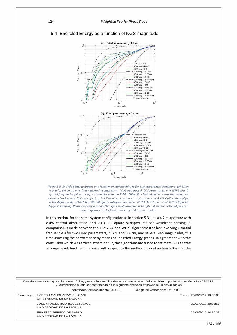
124 / 166
Este documento incorpora firma electrónica, y es copia auténtica de un documento electrónico archivado por la ULL según la Ley 39/2015.Su autenticidad puede ser contrastada en la siguiente dirección https://sede.ull.es/validacion/
Identificador del documento: 960521Código de verificación: ThtRedGl
Firmado por: HARESH MANGHARAM CHULANI Fecha: 23/06/2017 18:03:30UNIVERSIDAD DE LA LAGUNA
JOSE MANUEL RODRIGUEZ RAMOS 23/06/2017 18:06:55UNIVERSIDAD DE LA LAGUNA
ERNESTO PEREDA DE PABLO 27/06/2017 14:59:25UNIVERSIDAD DE LA LAGUNA
124 Weighted Fourier Phase Slope
5.4. Encircled Energy as a function of NGS magnitude
Figure 5-8. Encircled Energy graphs as a function of star magnitude for two atmospheric conditions: (a) 21 cm r0 and (b) 8.4 cm r0; and three centroiding algorithms: TCoG (red traces), CC (green traces) and WFPS with 6 spatial frequencies (blue traces), all tuned to estimate G-Tilt. Diffraction limited and no correction cases are
shown in black traces. System’s aperture is 4.2 m wide, with a central obscuration of 8.4%. Optical throughput is the default unity. SHWFS has 20 x 20 square subapertures and a ~2.7” FoV in (a) or ~3.8” FoV in (b) with Nyquist sampling. Phase recovery is modal through pseudo-inverson with optimal method selected for each
star magnitude and a fixed number of 130 Zernike modes.
In this section, for the same system configuration as in section 5.3, i.e., a 4.2 m aperture with
8.4% central obscuration and 20 x 20 square subapertures for wavefront sensing, a
comparison is made between the TCoG, CC and WFPS algorithms (the last involving 6 spatial
frequencies) for two Fried parameters, 21 cm and 8.4 cm, and several NGS magnitudes, this
time assessing the performance by means of Encircled Energy graphs. In agreement with the
conclusion which was arrived at section 5.2, the algorithms are tuned to estimate G-Tilt at the
subpupil level. Another difference with respect to the methodology at section 5.3 is that the

125 / 166
Este documento incorpora firma electrónica, y es copia auténtica de un documento electrónico archivado por la ULL según la Ley 39/2015.Su autenticidad puede ser contrastada en la siguiente dirección https://sede.ull.es/validacion/
Identificador del documento: 960521Código de verificación: ThtRedGl
Firmado por: HARESH MANGHARAM CHULANI Fecha: 23/06/2017 18:03:30UNIVERSIDAD DE LA LAGUNA
JOSE MANUEL RODRIGUEZ RAMOS 23/06/2017 18:06:55UNIVERSIDAD DE LA LAGUNA
ERNESTO PEREDA DE PABLO 27/06/2017 14:59:25UNIVERSIDAD DE LA LAGUNA
Chapter 5. Numerical simulations at an entire pupil level 125
number of modes employed at the modal phase recovery has been fixed to 130. Finally, the
EE graph is computed over the PSF obtained by integration during 4 seconds of the light from
the whole pupil at the focal plane with an imager object (200 frames separated 20 miliseconds
from each other). System frequency, SHWFS’s fields of view and detector’s gain and noise
parameters, and modal phase recovery methods, are the same as in sections 5.2 and 5.3.
Results are shown in Figure 5-8 in a double logarithmic scale, with panel (a) corresponding to
the 21 cm r0 case and panel (b) corresponding to the 8.4 cm r0 case. TCoG results for various
NGS magnitudes are shown in red traces with different line styles; the same magnitudes and
line styles for the CC algorithm are shown in green traces; and blue traces are used for the
WFPS algorithm. For a comparison purpose, the diffraction limited case and the turbulence
uncompensated case are shown in black traces as best and worst limits, respectively.
Results are in good agreement with the Strehl Ratios shown in Figure 5-7. The CC and WFPS
algorithms show a similar performance, that outperforms the one shown by the TCoG
algorithm. For the 21 cm r0 case in panel (a), and for a bright NGS of magnitude 5, the
performace is similar for the three algorithms, with the red trace of the TCoG being right
below the green trace of the CC, and thus being not visible. For NGS magnitudes of 10.5, 11
and 11.5, the difference in performance becomes very noticeable, with TCoG reaching similar
levels of EE as CC and WFPS for a dimmer NGS, with a magnitude somewhere between 0.5
and 1 higher. For the 8.4 cm r0 case in panel (b), the EE is one order of magnitude lower than
in the 21 cm r0 case for FoV’s smaller than 0.1”, in agreement with the SR decrease. Here
again CC and WFPS allow for a dimmer NGS than the required by TCoG, with a magnitude
~0.5 to ~1 higher. It may seem that CC slightly outperforms WFPS, but this is only apparent
and due to the logarithmic abscissa scale. A more careful inspection of the figure reveals that
WFPS actually reaches higher EE values than CC does for higher than 0.15” FoV’s. It is the
author’s opinion that, as WFPS does not threshold the image and makes a better estimation
of G-Tilt than CC, it achieves PSF’s with more concentrated energies but less peak values, and
this translates into smaller EE values for the initial FoV’s around the PSF’s main lobe width
that give place to higher EE values when the FoV’s increase. This effect is more noticeable in
the 8.4 cm r0 case than in the 21 cm r0 case, such as the difference between G-Tilt and Z-Tilt
is higher for the first case than for the second.
5.5. Conclusions of the present chapter
The comparison in performance between the TCoG, CC and WFPS algorithms has been
translated from the SHWFS subpupil level to the whole pupil level, thus including fitting error
due to the pupil spatial sampling. The OOMAO tool has been used for this purpose, with some
extensions implemented by the author. Results are shown in the form of Strehl Ratios and
Encircled Energies as a function of NGS magnitudes.
There is a very good coincidence between the performances seen at subpupil and at pupil
level. In high light level scenarios, that is, when fitting error dominates, all the algorithms
perform similarly. When measurement noise at subpupil level dominates, that is, at low light
level scenarios, CC and WFPS allow to use dimmer NGS’s, of about ~0.6 to ~0.7 higher

126 / 166
Este documento incorpora firma electrónica, y es copia auténtica de un documento electrónico archivado por la ULL según la Ley 39/2015.Su autenticidad puede ser contrastada en la siguiente dirección https://sede.ull.es/validacion/
Identificador del documento: 960521Código de verificación: ThtRedGl
Firmado por: HARESH MANGHARAM CHULANI Fecha: 23/06/2017 18:03:30UNIVERSIDAD DE LA LAGUNA
JOSE MANUEL RODRIGUEZ RAMOS 23/06/2017 18:06:55UNIVERSIDAD DE LA LAGUNA
ERNESTO PEREDA DE PABLO 27/06/2017 14:59:25UNIVERSIDAD DE LA LAGUNA
126 Weighted Fourier Phase Slope
magnitudes, than the required by the TCoG algorithm, for a certain performance as measured
by a SR or an EE.
This study has been reported for a 4.2 m aperture with 8.4% central obscuration, which are
the William Herschel Telescope’s dimensions. A 20 x 20 matrix of square shaped subapertures
has been considered for wavefront measurement at the SHWFS. And two turbulence strength
conditions have been simulated: a 21 cm r0, equal to the subaperture side size, and an 8.4 cm
r0, 2.5 smaller than the subaperture side size. Open loop wavefront sensing has been
assumed. Other spatial sampling configurations were tested and also showed coherent
results, but are not shown here.
The WFPS’s capacity to tune itself for Z-Tilt or G-Tilt estimation has been taken advantage of
to assess the effect of such a choice over the wavefront estimation at the pupil level. It seems
that Z-Tilt estimation at the subpupil level leads to a modest increase in SR, and G-Tilt
estimation leads to an also modest increase in EE. Though this should be confirmed with more
extensive simulation, it has been used as a criterion for tuning all the algorithms when
obtaining the results of SR and EE.

127 / 166
Este documento incorpora firma electrónica, y es copia auténtica de un documento electrónico archivado por la ULL según la Ley 39/2015.Su autenticidad puede ser contrastada en la siguiente dirección https://sede.ull.es/validacion/
Identificador del documento: 960521Código de verificación: ThtRedGl
Firmado por: HARESH MANGHARAM CHULANI Fecha: 23/06/2017 18:03:30UNIVERSIDAD DE LA LAGUNA
JOSE MANUEL RODRIGUEZ RAMOS 23/06/2017 18:06:55UNIVERSIDAD DE LA LAGUNA
ERNESTO PEREDA DE PABLO 27/06/2017 14:59:25UNIVERSIDAD DE LA LAGUNA
Chapter 6. Laboratory tests
The present chapter presents the description and results of a modest laboratory test
conducted mainly in order to show the necessary basic steps to apply the WFPS algorithm in
a real case. It has been achieved by taking advantage of the laboratory setup of the EDiFiSE
(Equalized and Diffraction limited Field Spectrograph Experiment) project at the Technology
Division of the IAC (Instituto de Astrofísica de Canarias). This setup is not, in principle, thought
for centroiding methods characterization. However, tests have been conducted as far as the
system would allow and a very good coincidence with the numerical simulations is seen in the
sensitivity test results, thereby confirming that the real system’s geometry is correctly
characterized and paving the way for moving the WFPS algorithm from simulation into reality.
6.1. The EDiFiSE project
EDiFiSE is a prototype instrument in development at the IAC’s Technology Division, in which
the author has participated during the execution of the present work. It is a high resolution
integral field spectrograph intended for the observation of high-contrast objects as an
alternative to coronographs. For this purpose, it combines an Adaptive Optics (AO) system
and an Equalized Integral Field Unit (EIFU). It is designed to be tested at the GHRIL (Ground-
based High Resolution Imaging Laboratory) platform of the 4.2m William Herschel Telescope
(WHT) at the Roque de los Muchachos Observatory in the island of La Palma. A detailed
description of the instrument and its scientific goals can be found at García-Lorenzo et al,
2008.
The technologies under test are basically two. One is the Field Programmable Gate Array
(FPGA) as an electronic component to fully implement the wavefront sensing and control
computation of the AO system (Chulani et al, 2016). The other one is a fiber optics based EIFU
where the central fibers are intensity regulated with variable attenuators, thereby allowing
to decrease the contrast of bright objects with respect to its surroundings and to detect
nearby faint objects or structures.

128 / 166
Este documento incorpora firma electrónica, y es copia auténtica de un documento electrónico archivado por la ULL según la Ley 39/2015.Su autenticidad puede ser contrastada en la siguiente dirección https://sede.ull.es/validacion/
Identificador del documento: 960521Código de verificación: ThtRedGl
Firmado por: HARESH MANGHARAM CHULANI Fecha: 23/06/2017 18:03:30UNIVERSIDAD DE LA LAGUNA
JOSE MANUEL RODRIGUEZ RAMOS 23/06/2017 18:06:55UNIVERSIDAD DE LA LAGUNA
ERNESTO PEREDA DE PABLO 27/06/2017 14:59:25UNIVERSIDAD DE LA LAGUNA
128 Weighted Fourier Phase Slope
At present, the AO system has successfully been integrated at the IAC laboratory facilities,
and tested using the IAC’s Atmosphere and Telescope (IACAT) simulator (see Moreno-Raso et
al, 2010, for a description of this simulation facility).
6.2. The laboratory test
6.2.1. The laboratory setup
Figure 6-1. Diagram of the portion of the optical laboratory setup of the EDiFiSE project which has been employed for the laboratory test in the present work.
Figure 6-1 is a diagram of the portion of EDiFiSE’s laboratory optical setup which has been
employed in the present work. The IACAT simulator is provided with a regulatable light source
that feeds with white light a pinholes plate through optical fibers, thus being able to simulate
a single Natural Guide Star (NGS) or an asterism. Five phase plates that emulate Kolomogorov
turbulence are available, each with a different Fried parameter. Upto three of them can be
simultaneously motorized and mounted on the optical bench. Light is collimated and passed
through these phase plates and a 2 cm circular mask emulating the system’s aperture and
secondary’s central obscuration, till the telescope simulator. The characteristics of the WHT
have been selected, with a focal ratio f/10.94.
EDiFiSE’s AO system comprises two full-FPGA parallel control closed-loops, one for tip/tilt (TT)
correction and the other for higher order modes correction. The former has the S-330.2SL TT
platform and mirror from Physik Instrumente (PI) as the corrective element, whereas the
latter employs the DM97-15 deformable mirror (DM) from the Alpao manufacturer. Closed
loop correction means that these corrective elements come before the sensing elements in
the optical path. Hence, Figure 6-1 shows the Shack-Hartmann wavefront sensor (SHWFS) at
IACAT
Alpao
DM97-15
SHWFS
(based on Andor
iXon 860)
Phase
plates
20 mm
mask
Regulatable
Light Source
Pinholes plate
F/OCommon
collimator
Telescope
simulator
Instrument
collimator
(F 125 mm)
PI S-330.2SL
TT platform
+ mirror
(F 250 mm)
(F 60 mm)

129 / 166
Este documento incorpora firma electrónica, y es copia auténtica de un documento electrónico archivado por la ULL según la Ley 39/2015.Su autenticidad puede ser contrastada en la siguiente dirección https://sede.ull.es/validacion/
Identificador del documento: 960521Código de verificación: ThtRedGl
Firmado por: HARESH MANGHARAM CHULANI Fecha: 23/06/2017 18:03:30UNIVERSIDAD DE LA LAGUNA
JOSE MANUEL RODRIGUEZ RAMOS 23/06/2017 18:06:55UNIVERSIDAD DE LA LAGUNA
ERNESTO PEREDA DE PABLO 27/06/2017 14:59:25UNIVERSIDAD DE LA LAGUNA
Chapter 6. Laboratory tests 129
the end of the optical path. This WFS comprises an array of square microlenses and an EMCCD
(Electronic Multiplication Charge Coupled Device) Andor iXon 860 detector. An instrument
collimator lens with 125 mm focal length at the instrument’s interface with the IACAT creates
a ~11.43 mm wide collimated beam that incides on the corrective elements, and which is
further reduced by the pair of lenses with 250 and 60 mm focal lengths, in order to fit into
the SHWFS detector size, which is ~3.07 mm in size per side (the detector comprises 128 x
128 pixels and pixel size is 24 x 24 microns). The square microlens size is ~310 microns per
side, and so we have a 10 x 10 subpupils SHWFS configuration for a 4.2 m aperture telescope.
Figure 6-1 is a simplified diagram of the laboratory setup, with the necessary components to
explain the test performed in the context of this work. Just to give the reader an idea of the
real appearance of the setup, Figure 6-2 is a shot of the same from a nice viewpoint, courtesy
by Dr. Félix Gracia Témich, from the EDiFiSE project team. In the foreground, the SHWFS
components, i.e., the Andor iXon 860 detector and the microlens array mechanical mount are
shown. In the middle ground, the two corrective elements can be seen, that is, the Alpao’s
DM and the TT platform from PI. The Kolmogorov phase plates are situated in the background
of the photograph.
Figure 6-2. View of the optical setup of the EDiFiSE project at the laboratory facilities of the IAC, courtesy by Dr. Félix Gracia Temich, from the EDiFiSE team.
6.2.2. Description of the test
As it was said in the introduction of this chapter, the described setup in the previous point is
not meant for centroiding methods performance assessment. First of all, the optical path
spans a portion of the phase plates, and there is not any means of knowing the true applied

130 / 166
Este documento incorpora firma electrónica, y es copia auténtica de un documento electrónico archivado por la ULL según la Ley 39/2015.Su autenticidad puede ser contrastada en la siguiente dirección https://sede.ull.es/validacion/
Identificador del documento: 960521Código de verificación: ThtRedGl
Firmado por: HARESH MANGHARAM CHULANI Fecha: 23/06/2017 18:03:30UNIVERSIDAD DE LA LAGUNA
JOSE MANUEL RODRIGUEZ RAMOS 23/06/2017 18:06:55UNIVERSIDAD DE LA LAGUNA
ERNESTO PEREDA DE PABLO 27/06/2017 14:59:25UNIVERSIDAD DE LA LAGUNA
130 Weighted Fourier Phase Slope
phase therefrom, such as a second SHWFS with a very high spatial resolution. Second, the
system was not designed to automatically acquire SHWFS image sequences with a varying
atmospheric phase in a repetitive manner and with different light levels. The light source is
manually regulatable through a knob, and the phase plates control software and SHWFS data
acquisition software are not interconnected. An automated system would have facilitated to
make statistics from acquired image sequences. However, it was out of the scope of the
present work to develop such a system. And third, the optical setup is that of a closed-loop
controlled system, and the SHWFS has been configured for such a control mode. The
microlenses’ focal length is ~25 mm, giving a spot FWHM size at diffraction limit of ~2.5
pixels. The assigned portion of the detector to each subpupil can be at most 12 x 12 pixels,
which is good enough for closed loop control, but unsufficient for open loop sensing with such
a big spot when the Fried parameter goes below the subaperture side size. This leaves no
margin at all for FoV variation assessment tests.
Bearing in mind the mentioned limitations, a test has been designed to assess the sensitivity
performance of the WFPS centroiding method against the TCoG and CC algorithms. The
corrective elements have been employed as passive reflectors, only giving the DM the
necessary shape to compensate for static aberrations in the optical path from the light source
to the SHWFS (leaving the phase plates aside). Therefore, wavefront sensing has been as in
an open loop mode. The phase plates have been kept still, thus emulating a static atmospheric
aberration. For every static aberration emulated, SHWFS image sequences of 5000 frames
have been taken, each with a different light source level. Also, accumulations of 10000 frames
with the same light levels have been taken, in order to assess the incident light level per
subpupil in the SHWFS. The acquired image sequences have been processed offline in order
to assess the wavefront sensing degradation as the light level decreases. This has been done
with all the centroiding methods under evaluation: the TCoG, the CC, and the WFPS with the
six lowermost spatial frequencies involved and two 2D-FFT sizes, 12 x 12 and 14 x 14. A
reasonable and fair estimation of the true applied phase has been considered to be at the
halfway in the range between the minimum and maximum coordinate values for each
centroid at each subpupil15, dealing separately with horizontal and vertical coordinates,
computed over the accumulated frame with the highest light level.
The tuning of all the centroiding methods has been aimed to estimate Z-Tilt, and has been
done by simulating the real system’s geometry at a subpupil level. In this regard, two are the
main system parameters that need to be determined: the Fried parameter and the FWHM of
the diffraction spot at the subpupil in pixel units.
Three have been the static turbulent aberrations emulated and, so, three have been the Fried
parameter values to determine. In the first case, a single plate has been used which the
manufacturer specifies as having a phase drawing with r0 = 2.32 mm at λ = 632nm, which
scales to a 48.7 cm r0 at the WHT (the Fried parameter values of the phase plates and their
combinations, scaled to the WHT, have been taken from Fuensalida, 2015). The Andor iXon
860 quantum efficiency curve shows a pass band centered at 600 nm, and for this wavelength
15 As some philosophical currents would state, virtue is in the midpoint between all extremes.

131 / 166
Este documento incorpora firma electrónica, y es copia auténtica de un documento electrónico archivado por la ULL según la Ley 39/2015.Su autenticidad puede ser contrastada en la siguiente dirección https://sede.ull.es/validacion/
Identificador del documento: 960521Código de verificación: ThtRedGl
Firmado por: HARESH MANGHARAM CHULANI Fecha: 23/06/2017 18:03:30UNIVERSIDAD DE LA LAGUNA
JOSE MANUEL RODRIGUEZ RAMOS 23/06/2017 18:06:55UNIVERSIDAD DE LA LAGUNA
ERNESTO PEREDA DE PABLO 27/06/2017 14:59:25UNIVERSIDAD DE LA LAGUNA
Chapter 6. Laboratory tests 131
the r0 decreases to ~45.75 cm. Finally, the subaperture size to Fried parameter ratio has been
approximated to unity: D/r0 ~ 1. For the second case, a single plate has been used as well,
with a drawing r0 of 1.36 mm at λ = 632 nm. This scales to an r0 = ~26.87 cm at λ = 600 nm at
the WHT, and the approximation of D/r0 ~ 1.5 has been made. As for the third turbulence
case, the combination of the two previous plates has been used, which gives a Fried
paramenter value r0 = ~21.9 cm at λ = 600 nm at the WHT, and D/r0 has been approximated
to ~2. The last two cases correspond to Fried parameter values of ~21.6 cm and ~17.6 cm at
a 500 nm wavelength, which would be good seeing situations at the Roque de los Muchachos
Observatory in La Palma. Smaller r0’s would have required a larger FoV than the available one
to deal with the spots’ tilt.
As regards the FWHM size, the actual value sought is the λ/D ratio, with D being the square
subaperture side size. For a 600 nm wavelength and a 42 cm subaperture side size, the λ/D
ratio is ~0.295”. The scale plate at the SHWFS is ~0.129”/pixel, and so the value in pixels of
the the λ/D ratio is ~2.3. When illuminating the SHWFS with a flat wavefront, somewhat
wider spots were seen, perhaps due to the effect of the higher wavelengths in the white light,
and FWHM values ~2.7 - 2.9 pixels were obtained when fitting the spots to 2D Gaussian
shapes. Finally, a 2.5 pixels value has been selected for the λ/D ratio in the simulation, which
corresponds to a ~650 nm wavelength. This has been obtained at the simulation by assigning
a 32 x 32 pixels resolution to the square subpupil, and employing an 80 x 80 2D-FFT to obtain
the Fraunhofer image at the focal plane (see equation [Eq. 4-16]). Out of the full image
obtained, a 12 x 12 pixels central portion is finally selected.
The other simulation parameters of importance are related to the detector sensitivity, gain
and noise values. A sensitivity value of 16 e-/ADU has been introduced in the simulation. The
real EMCCD gain has been seen to be a ~20% lower than the programmed gain with the
detector’s cooling system set at -80ºC. Two gain values were programmed: 1000 for light
levels below 1000 incident photons per subpupil, and 200 for higher levels. So, the values
introduced in the simulation have been 800 and 160, respectively. As for the noises, a CIC
value of 0.155 e-/pixel/frame and a RON of 50 rms e- have been employed. Appendix B details
how these values have been determined.
6.2.3. Test results
Having estimated the true phase for each of the three static turbulences applied as that
obtained over the accumulation of frames with the highest light level, i.e., in a negligible
detector noise situation, and as a fair compromise between all the centroiding methods, it is
possible to estimate the phase error for every acquired frame in every sequence at each light
level. This phase error has been first estimated at a subpupil level, as a difference in centroid
coordinates at each subpupil. The rms value of such estimated phase tilt error throughout the
whole image sequence, averaged among all the centroids in the image, is represented for
each light level in panels labelled (a) of Figures 6-3, 6-4 and 6-5, for the three turbulence
phases applied and the four centroid algorithms under evaluation. The units have been
converted from rms pixels to rms tilt radians applying equation [Eq. 4-25].

132 / 166
Este documento incorpora firma electrónica, y es copia auténtica de un documento electrónico archivado por la ULL según la Ley 39/2015.Su autenticidad puede ser contrastada en la siguiente dirección https://sede.ull.es/validacion/
Identificador del documento: 960521Código de verificación: ThtRedGl
Firmado por: HARESH MANGHARAM CHULANI Fecha: 23/06/2017 18:03:30UNIVERSIDAD DE LA LAGUNA
JOSE MANUEL RODRIGUEZ RAMOS 23/06/2017 18:06:55UNIVERSIDAD DE LA LAGUNA
ERNESTO PEREDA DE PABLO 27/06/2017 14:59:25UNIVERSIDAD DE LA LAGUNA
132 Weighted Fourier Phase Slope
The commands to the DM are calculated through MVM (Matrix Vector Multiplication) in the
control loops in normal operation of the AO system of EDiFiSE. The same control matrixes
have been employed to estimate the phase errors at the complete pupil. True phases have
been estimated in the same manner as for the subpupil tilts, i.e., as a midpoint in the range
of phases corresponding to the different centroiding methods for every DM actuator,
obtained from the accumulated frame at the highest light level for each static turbulence
applied. The phase at the pupil is then obtained for each frame, as corrective commands to
the DM, by applying the control matrix to the obtained centroids vector, and the phase error
is obtained at every DM actuator as the distance between its phase and the estimated true
phase. The rms values of such distances throughout the whole image sequence, averaged
among all the DM actuators, is represented for each light level in panels labelled (b) of Figures
6-3, 6-4 and 6-5, for the three turbulence phases applied and the four centroiding algorithms.
As the fitting error is not actually being taken into account, the graph shapes are very similar
to those in panels (a). The units are in rms percentage of peak to valley (PV) stroke at the DM.
According to the manufacturer, the 100% PV stroke cannot be specified in length units as it
depends on the mirror shape. The author estimates it should be around ~10 – 20 microns16.
Figure 6-3 shows the results for the D/r0 ~ 1 case. This turbulence phase has produced the
least clear results among the three studied cases. As it was seen in chapter 4, the better the
turbulence condition, the less difference will be appreciated between the different
centroiding methods. In spite of this, the tendency of the TCoG algorithm to worsen its tilt
estimation more rapidly than the other algorithms as the light decreases below 200 incident
photons per subpupil is clearly seen in the figure. For higher light levels, the variation of all
the centroiding methods with light level is similar. Note that these values should not be
interpreted as tilt or phase estimation errors and used to compare the tilt or phase estimation
capacity of each centroiding method, since they are actually distances to a midpoint which
has been taken as a true phase. Centroiding methods that obtain an estimation which is closer
to this midpoint will show lower values in the graph, but this does not mean a better
estimation of the real phase. So, the graphs should only be used to corroborate that there is
not much dispersion between the different methods at high light level, which is the case (0.1
rms radians is ~λ/60); and to evaluate the estimated tilt variation as light decreases for every
algorithm in order to assess its sensitivity.
Figure 6-4, for a D/r0 ~ 1.5 case, shows a much clearer result than the previous one, perhaps
because this phase had a strong tilt component, and the errors at low light level reach values
which are more than double of those shown in the previous figure. Here, the difference in
sensitivity of the TCoG algorithm with respect to the other algorithms is very visible, and the
gap in estimated tilt between 20 and 200 incident photons per subpupil reminds the results
obtained by simulation at a subpupil level in chapter 4. Similar comments can be said of the
results shown in Figure 6-5 for the D/r0 ~ 2 case, which confirm the improvement in sensitivity
of the WFPS and CC algorithms with respect to the TCoG.
16 From DM stroke specifications at the Alpao’s web page for different Zernike modes.
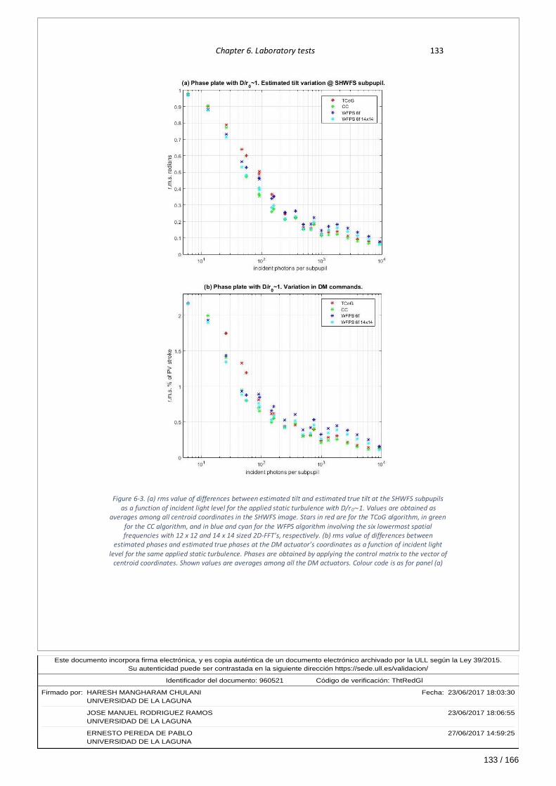
133 / 166
Este documento incorpora firma electrónica, y es copia auténtica de un documento electrónico archivado por la ULL según la Ley 39/2015.Su autenticidad puede ser contrastada en la siguiente dirección https://sede.ull.es/validacion/
Identificador del documento: 960521Código de verificación: ThtRedGl
Firmado por: HARESH MANGHARAM CHULANI Fecha: 23/06/2017 18:03:30UNIVERSIDAD DE LA LAGUNA
JOSE MANUEL RODRIGUEZ RAMOS 23/06/2017 18:06:55UNIVERSIDAD DE LA LAGUNA
ERNESTO PEREDA DE PABLO 27/06/2017 14:59:25UNIVERSIDAD DE LA LAGUNA
Chapter 6. Laboratory tests 133
Figure 6-3. (a) rms value of differences between estimated tilt and estimated true tilt at the SHWFS subpupils as a function of incident light level for the applied static turbulence with D/r0~1. Values are obtained as
averages among all centroid coordinates in the SHWFS image. Stars in red are for the TCoG algorithm, in green for the CC algorithm, and in blue and cyan for the WFPS algorithm involving the six lowermost spatial frequencies with 12 x 12 and 14 x 14 sized 2D-FFT’s, respectively. (b) rms value of differences between
estimated phases and estimated true phases at the DM actuator’s coordinates as a function of incident light level for the same applied static turbulence. Phases are obtained by applying the control matrix to the vector of
centroid coordinates. Shown values are averages among all the DM actuators. Colour code is as for panel (a)
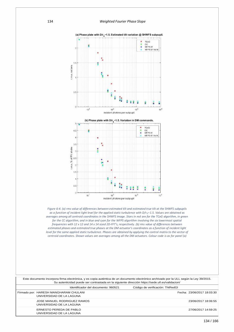
134 / 166
Este documento incorpora firma electrónica, y es copia auténtica de un documento electrónico archivado por la ULL según la Ley 39/2015.Su autenticidad puede ser contrastada en la siguiente dirección https://sede.ull.es/validacion/
Identificador del documento: 960521Código de verificación: ThtRedGl
Firmado por: HARESH MANGHARAM CHULANI Fecha: 23/06/2017 18:03:30UNIVERSIDAD DE LA LAGUNA
JOSE MANUEL RODRIGUEZ RAMOS 23/06/2017 18:06:55UNIVERSIDAD DE LA LAGUNA
ERNESTO PEREDA DE PABLO 27/06/2017 14:59:25UNIVERSIDAD DE LA LAGUNA
134 Weighted Fourier Phase Slope
Figure 6-4. (a) rms value of differences between estimated tilt and estimated true tilt at the SHWFS subpupils as a function of incident light level for the applied static turbulence with D/r0~1.5. Values are obtained as
averages among all centroid coordinates in the SHWFS image. Stars in red are for the TCoG algorithm, in green for the CC algorithm, and in blue and cyan for the WFPS algorithm involving the six lowermost spatial frequencies with 12 x 12 and 14 x 14 sized 2D-FFT’s, respectively. (b) rms value of differences between
estimated phases and estimated true phases at the DM actuator’s coordinates as a function of incident light
level for the same applied static turbulence. Phases are obtained by applying the control matrix to the vector of centroid coordinates. Shown values are averages among all the DM actuators. Colour code is as for panel (a)

135 / 166
Este documento incorpora firma electrónica, y es copia auténtica de un documento electrónico archivado por la ULL según la Ley 39/2015.Su autenticidad puede ser contrastada en la siguiente dirección https://sede.ull.es/validacion/
Identificador del documento: 960521Código de verificación: ThtRedGl
Firmado por: HARESH MANGHARAM CHULANI Fecha: 23/06/2017 18:03:30UNIVERSIDAD DE LA LAGUNA
JOSE MANUEL RODRIGUEZ RAMOS 23/06/2017 18:06:55UNIVERSIDAD DE LA LAGUNA
ERNESTO PEREDA DE PABLO 27/06/2017 14:59:25UNIVERSIDAD DE LA LAGUNA
Chapter 6. Laboratory tests 135
Figure 6-5. (a) rms value of differences between estimated tilt and estimated true tilt at the SHWFS subpupils as a function of incident light level for the applied static turbulence with D/r0~2. Values are obtained as
averages among all centroid coordinates in the SHWFS image. Stars in red are for the TCoG algorithm, in green for the CC algorithm, and in blue and cyan for the WFPS algorithm involving the six lowermost spatial frequencies with 12 x 12 and 14 x 14 sized 2D-FFT’s, respectively. (b) rms value of differences between
estimated phases and estimated true phases at the DM actuator’s coordinates as a function of incident light level for the same applied static turbulence. Phases are obtained by applying the control matrix to the vector of
centroid coordinates. Shown values are averages among all the DM actuators. Colour code is as for panel (a)

136 / 166
Este documento incorpora firma electrónica, y es copia auténtica de un documento electrónico archivado por la ULL según la Ley 39/2015.Su autenticidad puede ser contrastada en la siguiente dirección https://sede.ull.es/validacion/
Identificador del documento: 960521Código de verificación: ThtRedGl
Firmado por: HARESH MANGHARAM CHULANI Fecha: 23/06/2017 18:03:30UNIVERSIDAD DE LA LAGUNA
JOSE MANUEL RODRIGUEZ RAMOS 23/06/2017 18:06:55UNIVERSIDAD DE LA LAGUNA
ERNESTO PEREDA DE PABLO 27/06/2017 14:59:25UNIVERSIDAD DE LA LAGUNA
136 Weighted Fourier Phase Slope
6.3. Conclusions of this chapter
A test has been conducted at the laboratory facilities of the IAC taking advantage of the AO
subsystem setup of the EDiFiSE project.
The results show, in the first place, that the method of determining the WFPS Bayesian
weights, i.e., of tuning the algorithm, by simulating the real system’s geometry at a subpupil
level, is correct. This has been deducted from the similarity in tilt estimation results of the
WFPS algorithm and the control algorithms, the TCoG and the CC, at high light level.
And in the second place, a very good coincidence between the laboratory test and the
simulation at subpupil level has been found as regards the sensitivity performance of the
algorithms under evaluation, which confirms the improvement in performance of the WFPS
algorithm over the TCoG algorithm for light levels of 20 to 200 incident photons per subpupil,
in a very similar manner as the CC algorithm does.
This test has been conducted with three values of turbulence strength, leading to D/r0~1,
D/r0~1.5 and D/r0~2 ratio values, with D being the square subaperture size, and with a single
sample of static turbulence phase for each r0. Wavefronts have been sensed as in an open
loop correction mode. The FWHM of the SHWFS subpupil’s spot at diffraction limit has been
estimated as 2.5 pixels, and the FoV size has been 12 x 12 pixels.

137 / 166
Este documento incorpora firma electrónica, y es copia auténtica de un documento electrónico archivado por la ULL según la Ley 39/2015.Su autenticidad puede ser contrastada en la siguiente dirección https://sede.ull.es/validacion/
Identificador del documento: 960521Código de verificación: ThtRedGl
Firmado por: HARESH MANGHARAM CHULANI Fecha: 23/06/2017 18:03:30UNIVERSIDAD DE LA LAGUNA
JOSE MANUEL RODRIGUEZ RAMOS 23/06/2017 18:06:55UNIVERSIDAD DE LA LAGUNA
ERNESTO PEREDA DE PABLO 27/06/2017 14:59:25UNIVERSIDAD DE LA LAGUNA
Chapter 7. General conclusions and future work
7.1. General conclusions
Shack-Hartmann wavefront sensors (SHWFS) are by far the most commonly used wavefront
sensors in astronomy, and those with the most matured and known techonology. However,
they face new challenges as adaptive optics (AO) systems evolve. Recent Multi Object
Adaptive Optics (MOAO) systems work in open loop correction mode, and present their
sensors the need to balance sensitivity in low light level conditions with a large dynamic range
that copes with the uncorrected atmospheric turbulence. This requirement falls directly upon
the centroiding method employed at the subpupil of the SHWFS, and invites new studies and
proposals on this subject. This work presents a novel, optimized, Fourier domain based
centroiding method which is real time implementable. The following are the main conclusions
which can be extracted from this work.
1. A new centroiding method for SHWFS’s has been formulated, as a Bayesian estimator
of the tilt at the subpupil, from the image’s Fourier phase slopes. Phase slopes are
obtained without phase computation and unwrapping, and the computational cost is
one order of magnitude lower than for the Cross-Correlation (CC) algorithm. Its
applicability to wavefront sensing with point-like guiding souces has been shown. It
has been named Weighted Fourier Phase Slope (WFPS).
2. Numerical simulations both at the subpupil and at the pupil level, as well as
experimental results at the laboratory, show that the WFPS and CC algorithms have a
similar sensitivity, which outperforms the Thresholded Centre of Gravity (TCoG)
algorithm, for light levels in the range of 20 to 200 incident photons per subpupil and
in the presence of detector noises and turbulence high order perturbations. Sky
coverage is thus improved, as the NGS can be magnitude 0.6 – 0.7 higher

138 / 166
Este documento incorpora firma electrónica, y es copia auténtica de un documento electrónico archivado por la ULL según la Ley 39/2015.Su autenticidad puede ser contrastada en la siguiente dirección https://sede.ull.es/validacion/
Identificador del documento: 960521Código de verificación: ThtRedGl
Firmado por: HARESH MANGHARAM CHULANI Fecha: 23/06/2017 18:03:30UNIVERSIDAD DE LA LAGUNA
JOSE MANUEL RODRIGUEZ RAMOS 23/06/2017 18:06:55UNIVERSIDAD DE LA LAGUNA
ERNESTO PEREDA DE PABLO 27/06/2017 14:59:25UNIVERSIDAD DE LA LAGUNA
138 Weighted Fourier Phase Slope
3. As a consequence of the improved sensitivity, the algorithm’s optimal working FoV is
higher than for the TCoG algorithm, and similar to the CC algorithm’s, becoming an
algorithm of choice when large FoV’s are required, such as in open loop sensing and
in strong turbulence conditions. This point, and the following, have been shown
through numerical simulations at the subpupil level.
4. The WFPS algorithm keeps a relationship with low pass cepstrum filtering, and it can
be tuned to estimate Z-Tilt or G-Tilt in the presence of noise, without thresholding the
image at any step. As a consequence, it outperforms the CC and TCoG algorithms when
estimating G-Tilt at high light level and large enough FoV, for it can take into account
the low light level portion at the skirt of the spot.
5. As for Z-Tilt estimation at high light level, the three algorithms, TCoG, CC and WFPS,
perform similarly as long as a large enough FoV is spanned so as to avoid spot’s
truncation. In the case of a smaller FoV, and since the WFPS algorithm does not
threshold the image, it will need to employ a larger 2D-FFT than the image size in order
to simmetrize the spot and compensate for its partial truncation.
7.2. Future work
The following natural step is the algorithm verification in a fully operational adaptive optics
system at the lab, and then at a telescope. The necessary steps to achieve this goal would be:
1. The values of real world systems’ defining parameters constantly vary in time. In long
term observations, the turbulence Fried parameter, and even the received light from
the guiding source, change. It would be necessary therefore to devise a means to
adapt the algorithm (its Bayesian weights) to this changing working environment.
Further simulations are necessary in this line to determine the algorithm’s
performance degradation when utilizing non-optimal weights, so as to establish the
weights update period in long term real observations.
2. It has been seen that this algorithm shows an important advantage over the CC as
regards computational cost. This is based upon the computation of partial 2D-FFT’s,
i.e., their computation at only a limited number of spatial frequencies. It becomes
therefore necessary to efficiently programme this partial bi-dimensional discrete
Fourier transform computation for its execution in the platforms of choice of the AO
systems at the telescopes: CPU’s, GPU’s, FPGA’s, etc.
The variation in computational cost with respect to existing centroiding algorithms
should then be measured. This variation will probably require a tuning of the
stabilizing filters at the correction loops of the AO systems.

139 / 166
Este documento incorpora firma electrónica, y es copia auténtica de un documento electrónico archivado por la ULL según la Ley 39/2015.Su autenticidad puede ser contrastada en la siguiente dirección https://sede.ull.es/validacion/
Identificador del documento: 960521Código de verificación: ThtRedGl
Firmado por: HARESH MANGHARAM CHULANI Fecha: 23/06/2017 18:03:30UNIVERSIDAD DE LA LAGUNA
JOSE MANUEL RODRIGUEZ RAMOS 23/06/2017 18:06:55UNIVERSIDAD DE LA LAGUNA
ERNESTO PEREDA DE PABLO 27/06/2017 14:59:25UNIVERSIDAD DE LA LAGUNA
Chapter 7. General conclusions and future work 139
3. Appropriate working AO systems should be sought, such as MOAO systems that
correct in open loop, in order to test the algorithm’s performance against the
traditional ones, first at the lab and then at telescopes.
Moving on to another issue, throughout this work only point-like guiding sources have been
considered. However, the applicability of the algorithm in the field of AO for astronomy is
broader:
1. Firstly, the WFPS algorithm, such as it has been formulated in this work, is applicable
to wavefront sensing with LGS’s, where spots are seen elongated at the SHWFS’s
subpupils. This should be confirmed by numerical simulations first, determining the
2D-FFT required sizes, number of spatial frequencies involved, optimal weights, etc.
Elongated spots mean big required working FoV’s and large number of pixels per
subpupil involved, even in closed loop correction mode, and this is where the WFPS
algorithm outperforms the traditional CoG based ones. Also, its simmetrizing capacity
could be of advantage when the source is asymmetric right from the start.
2. Second, if the elongated spot’s structure should be taken into account, then the WFPS
algorithm could be reformulated as a weighted average of differences of Fourier phase
slopes corresponding to the live images and a reference image. This is applicable also
to the wavefront sensing with extended objects such as in solar AO. The effectiveness
first, and then the performance of this reformulated WFPS algorithm should be shown
through numerical simulations in principle. A possible advantage over the traditional
CC algorithm could be a considerable decrease in computational cost, as it has been
seen in this work.

140 / 166
Este documento incorpora firma electrónica, y es copia auténtica de un documento electrónico archivado por la ULL según la Ley 39/2015.Su autenticidad puede ser contrastada en la siguiente dirección https://sede.ull.es/validacion/
Identificador del documento: 960521Código de verificación: ThtRedGl
Firmado por: HARESH MANGHARAM CHULANI Fecha: 23/06/2017 18:03:30UNIVERSIDAD DE LA LAGUNA
JOSE MANUEL RODRIGUEZ RAMOS 23/06/2017 18:06:55UNIVERSIDAD DE LA LAGUNA
ERNESTO PEREDA DE PABLO 27/06/2017 14:59:25UNIVERSIDAD DE LA LAGUNA

141 / 166
Este documento incorpora firma electrónica, y es copia auténtica de un documento electrónico archivado por la ULL según la Ley 39/2015.Su autenticidad puede ser contrastada en la siguiente dirección https://sede.ull.es/validacion/
Identificador del documento: 960521Código de verificación: ThtRedGl
Firmado por: HARESH MANGHARAM CHULANI Fecha: 23/06/2017 18:03:30UNIVERSIDAD DE LA LAGUNA
JOSE MANUEL RODRIGUEZ RAMOS 23/06/2017 18:06:55UNIVERSIDAD DE LA LAGUNA
ERNESTO PEREDA DE PABLO 27/06/2017 14:59:25UNIVERSIDAD DE LA LAGUNA
Bibliography
Andersen D. et al, 2014. “Comparing the performance of open loop centroiding techniques in
the Raven MOAO system”, Adaptive Optics Systems IV, Proc. SPIE 9148.
Arines J. and Ares J., 2002. “Minimum variance centroid thresholding”, Optics Letters, Vol 27,
No 7, pp. 497-499.
Assémat F., Gendron E. and Hammer F., 2007. “The FALCON concept: multi-object adaptive
optics and atmospheric tomography for integral field spectroscopy – principles and
performance on an 8-m telescope”, Mon. Not. R. Astron. Soc. 376, pp. 287-312.
Carmon Y. and Ribak E. N., 2003. “Phase retrieval by demodulation of a Hartmann-Shack
sensor”, Optics Communications, 215, pp. 285-288.
Chulani H. M. and Rodríguez-Ramos J. M., 2013. “Weighted Fourier Phase Slope as a
centroiding method in a Shack-Hartmann wavefront sensor: A Z-tilt estimation
method in the Fourier domain, optimizable to the system’s geometry”, IEEE 12th
Workshop on Information Optics (WIO’2013).
Chulani H.M. et al, 2016. “EDIFISE full-FPGA adaptive optics. First laboratory results using the
IACAT optical ground support equipment”, Adaptive Optics Systems V, Proc. SPIE
9909.
Chulani H. M. and Rodríguez-Ramos J. M., 2017. “Preliminary performance results of the
Weighted Fourier Phase Slope centroiding method for Shack Hartmann wavefront
sensors obtained with the OOMAO simulator”, accepted for presentation at the 5th
Adaptive Optics for Extremely Large Telescopes (AO4ELT5) Conference.
Conan R. and Correia C., 2014. “Object-oriented Matlab adaptive optics toolbox”, Adaptive
Optics Systems IV, Proc. SPIE 9148.
Fillard J.P., 1992. “Subpixel accuracy location estimation from digital signals”, Optical
Engineering, Vol 31, No 11, pp. 2465-2471.
Fillard J.P. et al, 1993. “Computer simulation of super-resolution point source image
detection”, Optical Engineering, Vol 32, No 11, pp. 2936-2944.
Fried, D.L., 1965. “Statistics of a Geometric Representation of Wavefront Distortion”, J. Opt.
Soc. Am. 55(11), pp. 1427-1435.
Fried, D.L., 1977. “Least-square fitting a wave-front distortion estimate to an array of phase-
difference measurements”, J. Opt. Soc. Am., Vol 67, No 3, pp. 370-375.
Fuensalida J. J., 2015. “Combinación de placas de fase de IACAT en configuración WHT para
EDiFiSE”. IAC internal report. Ref. IP/TN-EDI/170.

142 / 166
Este documento incorpora firma electrónica, y es copia auténtica de un documento electrónico archivado por la ULL según la Ley 39/2015.Su autenticidad puede ser contrastada en la siguiente dirección https://sede.ull.es/validacion/
Identificador del documento: 960521Código de verificación: ThtRedGl
Firmado por: HARESH MANGHARAM CHULANI Fecha: 23/06/2017 18:03:30UNIVERSIDAD DE LA LAGUNA
JOSE MANUEL RODRIGUEZ RAMOS 23/06/2017 18:06:55UNIVERSIDAD DE LA LAGUNA
ERNESTO PEREDA DE PABLO 27/06/2017 14:59:25UNIVERSIDAD DE LA LAGUNA
142 Weighted Fourier Phase Slope
Fusco T. et al, 2004. “Optimisation of a Shack-Hartmann-based wavefront sensor for XAO
system”, Advancements in Adaptive Optics, Proc. SPIE 5490, pp. 1155-1166.
García-Lorenzo B. et al, 2008. “EDiFiSE: equalized and diffraction-limited field spectrograph
experiment”, Proc. SPIE 7014.
Gavel D., 2006. “Multi-Object Adaptive Optics and Multi-Conjugate Adaptive Optics
Architectures. System Design Trade Study.” Keck Next Generation Adaptive Optics.
Draft.
Ghiglia D.C. and Pritt M.D., 1998. “Two-Dimensional Phase Unwrapping: Theory, Algorithms
and Software”, New York: Wiley-Interscience.
Goldstein R.M., Zebken H.A. and Werner C.L., 1988. “Satellite radar interferometry: Two-
dimensional phase unwrapping”, Radio Science, Vol 23, No 4, pp. 713–720.
Goodman, J.W., 1985. “Statistical Optics”, John Wiley and Sons, New York, N.Y.
Goodman, J.W., 2005. “Introduction to Fourier Optics”, 3rd ed., Roberts & Co Publishers.
Gradatour D. et al, 2010. “Comparing centroiding methods for Shack-Hartmann wavefront
sensing with laser guide stars on an ELT”. Adaptive Optics Systems II, Proc. SPIE 7736.
Guzmán D. et al, 2010. “Deformable mirror model for open-loop adaptive optics using
multivariate adaptive regression splines”, Optics Express, Vol 18, No 7, pp. 6492-6505.
Hardy, J.W., 1998. “Adaptive Optics for Astronomical Telescopes”, New York, Oxford
University Press.
Hartmann J., 1900. “Bemerkungen über den Bau und die Justirung von Spectrographen”,
Zeitschrift für Instrumentenkunde, Berlin, Julins Springer, 20: 17-27, 47-58.
Herrmann J., 1980. “Least squares wave front errors of minimum norm”, J. Opt. Soc. Am., Vol
70, No 1, pp. 28-35.
Hirsch M. et al, 2013. “A Stochastic Model for Electron Multiplication Charge-Coupled Devices
– From Theory to Practice”, PLoS ONE, Vol 8, Issue 1: e53671.
Hudgin R.H., 1977. “Wavefront reconstruction for compensated imaging”, J. Opt. Soc. Am.,
Vol 67, No 3, pp. 375-378.
Kolmogorov, A., 1961. “The local structure of turbulence in incompressible viscous fluids for
very large Reynolds’ numbers”, Turbulence, Classic Papers on Statistical Theory, S. K.
Friedlander and L. Topper eds. Wiley-Interscience Publishers Inc., New York, NY.
Lardière O. et al, 2010. “Compared performance of different centroiding algorithms for high-
pass filtered laser guide star Shack-Hartmann wavefront sensors”, Adaptive Optics
Systems II, Proc. SPIE 7736.
Lardière O. et al, 2014. “Multi-Object Adaptive Optics On-sky Results with RAVEN”, Adaptive
Optics Systems IV, Proc. SPIE 9148.

143 / 166
Este documento incorpora firma electrónica, y es copia auténtica de un documento electrónico archivado por la ULL según la Ley 39/2015.Su autenticidad puede ser contrastada en la siguiente dirección https://sede.ull.es/validacion/
Identificador del documento: 960521Código de verificación: ThtRedGl
Firmado por: HARESH MANGHARAM CHULANI Fecha: 23/06/2017 18:03:30UNIVERSIDAD DE LA LAGUNA
JOSE MANUEL RODRIGUEZ RAMOS 23/06/2017 18:06:55UNIVERSIDAD DE LA LAGUNA
ERNESTO PEREDA DE PABLO 27/06/2017 14:59:25UNIVERSIDAD DE LA LAGUNA
Bibliography 143
Leroux C. and Dainty C., 2010. “Estimation of centroid positions with a matched filter
algorithm: relevance for aberrometry of the eye”, Optics Express, Vol 18, No 2, pp.
1197-1206.
Li T., Huang L. and Gong M., 2014. “Wavefront sensing for a nonuniform intensity laser beam
by Shack-Hartmann sensor with modified Fourier domain centroiding”, Optical
Engineering, Vol 53, No 4.
Lukin V.P. et al, 2010: “Wavefront sensors and algorithms for adaptive optical systems”,
Adaptive Optics System II, Proc. SPIE 7736.
Marlon V., 2014. “Investigación del problema inverso de reconstrucción tomográfica en
óptica adaptativa para astronomía a través de técnicas de minería de datos e
inteligencia artificial”, PhD Dissertation, Oviedo University, Spain.
Moreno-Raso J. et al, 2010. “Atmosphere and telescope simulator for new adaptive optics
methods development”, Adaptive Optics Systems II, Proc. SPIE 7736.
Nicolle M. et al, 2004. “Improvement of Shack-Hartmann wave-front sensor measurement for
extreme adaptive optics”, Optics Letters, Vol 29, No 23, pp. 2743-2745.
Noll, R.J., 1976. “Zernike polynomials and atmospheric turbulence”, J. Opt. Soc. Am., Vol 66,
No 3, pp. 207-211.
Oppenheim A. V. and Schafer R. W., 1989. “Discrete Time Signal Processing”, Prentice Hall
International, Inc.
Pinna F., 2014. “Modelado y caracterización de cámaras EMCCD (Electron Multiplication
Charge Coupled Devices) de uso en óptica adaptativa, a partir de un modelo
estocástico conocido de las mismas. Validación con imágenes reales.” IAC’s internal
report DE/PR-DE/033v.1.
Platt, B.C. and Shack, R.V., 2001. “History and Principles of Shack-Hartmann Wavefront
Sensing”, J. of Refractive Surgery, Vol 17, No 5, pp. S573-577.
Poyneer L.A. et al, 2005. “Experimental results for correlation-based wavefront sensing”,
Advanced Wavefront Control: Methods, Devices and Applications III, Proc. SPIE 5894.
Quirós F., 2007. “Reconstruction and Control Laws for Multi-conjugate Adaptive Optics in
Astronomy”, PhD Dissertation, Imperial College, London, UK.
Ragazzoni R., 1996. “Pupil plane wavefront sensing with an oscillating prism”, Journal of
Modern Optics, Vol 43, No 2, pp. 289-293.
Rigaut F.J., Ellerbroek B.L. and Flicker R., 2000. “Principles, limitations and performance of
multiconjugate adaptive optics”, Proc. SPIE Vol 4007, pp. 1022-1031.
Rigaut F., 2002. “Ground conjugate wide field adaptive optics for the ELTs”. Beyond
Conventional Adaptive Optics, ESO Conference and Workshop Proc., 58, pp.11-16.

144 / 166
Este documento incorpora firma electrónica, y es copia auténtica de un documento electrónico archivado por la ULL según la Ley 39/2015.Su autenticidad puede ser contrastada en la siguiente dirección https://sede.ull.es/validacion/
Identificador del documento: 960521Código de verificación: ThtRedGl
Firmado por: HARESH MANGHARAM CHULANI Fecha: 23/06/2017 18:03:30UNIVERSIDAD DE LA LAGUNA
JOSE MANUEL RODRIGUEZ RAMOS 23/06/2017 18:06:55UNIVERSIDAD DE LA LAGUNA
ERNESTO PEREDA DE PABLO 27/06/2017 14:59:25UNIVERSIDAD DE LA LAGUNA
144 Weighted Fourier Phase Slope
Robbins M.S. and Hadwen B.J., 2003. “The noise performance of Electron Multiplying Charge-
Coupled Devices”. IEEE Transactions on Electron Devices, Vol 50, No 5.
Roddier F., 1981. “The effects of atmospheric turbulence in optical astronomy”, Progress in
Optics XIX, E. Wolf eds., North Holland.
Roddier F., Roddier C. and Roddier N., 1988. “Curvature Sensing: A New Wavefront Sensing
Method”, Proc. SPIE Vol 0976, Statistical Optics.
Roddier N., 1990. “Atmospheric wavefront simulation and Zernike polynomials”, Proc. SPIE
Vol 1237, Amplitude and Intensity Spatial Interferometry, pp. 668-679.
Rodríguez-Ramos J.M., 1998. “Detección de frente de onda. Aplicación a técnicas de alta
resolución espacial y alineamiento de superficies ópticas segmentadas”, PhD
Dissertation, La Laguna University, Spain.
Rodriguez-Ramos J.M. et al, 2008: “2D-FFT implementation on FPGA for wavefront phase
recovery from the CAFADIS camera”, Adaptive Optics Systems, Proc. SPIE 7015.
Rousset G. et al, 2011. “First star images corrected by multi-object adaptive optics”, SPIE
Newsroom, DOI 10.1117/2.1201109.003736
Ruggiu J.M., Solomon C.J. and Loos G., 1998. “Gram-Charlier matched filter for Shack-
Hartmann sensing at low light levels”, Optics Letters, Vol 23, No 4, pp. 235-237.
Sallberg S.A., Welsh B.M. and Roggemann M.C., 1997. “Maximum a posteriori estimation of
wave-front slopes using a Shack-Hartmann wave-front sensor”, J. Opt. Soc. Am. A, Vol
14, No 6.
Sarver E.J., Schwiegerling J. and Applegate R.A., 2006. “Extracting Wavefront Error from
Shack-Hartmann Images Using Spatial Demodulation”. J. Refract. Surg., 22(9), pp. 949-
953.
Shack, R.V., 1971. “Production and use of a lenticular Hartmann screen”, J. Opt. Soc. Am. (Oral
presentation). Ramada Inn, Tucson, Arizona. Smith, F. Dow, ed. Vol 61, No 5, p. 656.
Sidick E. et al, 2008. “Adaptive cross-correlation algorithm for extended scene Shack-
Hartmann wavefront sensing”, Optics Letters, Vol 33, No 3, pp. 213-215.
Srinath M.D. and Rajasekaran P.K., 1979. “An Introduction to Statistical Signal Processing with
Applications”, John Wiley & Sons.
Stephenson P., 2014. “Recurrence relations for the Cartesian derivatives of the Zernike
polynomials”, J. Opt. Soc. Am. A, Vol 31, No 4, pp. 708-715.
Talmi A. and Ribak E.N., 2004. “Direct demodulation of Hartmann-Shack patterns”. J. Opt. Soc.
Am. A., Vol 21, No 4.
Tatarski, V.I., 1961. “Wave Propagation in a Turbulent Medium”, McGraw-Hill Book Company,
New York, NY.

145 / 166
Este documento incorpora firma electrónica, y es copia auténtica de un documento electrónico archivado por la ULL según la Ley 39/2015.Su autenticidad puede ser contrastada en la siguiente dirección https://sede.ull.es/validacion/
Identificador del documento: 960521Código de verificación: ThtRedGl
Firmado por: HARESH MANGHARAM CHULANI Fecha: 23/06/2017 18:03:30UNIVERSIDAD DE LA LAGUNA
JOSE MANUEL RODRIGUEZ RAMOS 23/06/2017 18:06:55UNIVERSIDAD DE LA LAGUNA
ERNESTO PEREDA DE PABLO 27/06/2017 14:59:25UNIVERSIDAD DE LA LAGUNA
Bibliography 145
Thomas S. et al, 2006: “Comparison of centroid computation algorithms in a Shack-Hartmann
sensor”, Mon. Not. R. Astron. Soc. 371, pp. 323-336.
Tyler G.A., 1994. “Bandwidth considerations for tracking through turbulence”, J. Opt. Soc. Am.
A, Vol 11, No 1, pp. 358-367.
Tyson, R.K., 1991. “Principles of Adaptive Optics”, Academic Press, New York.
Van Dam M.A. and Lane R.G., 2000. “Wave-front slope estimation”, J. Opt. Soc. Am. A, Vol 17,
No 7, pp. 1319-1324.
Vyas A., Roopashree M. B. and Prasad B. R., 2009(a). “Optimization of Existing Centroiding
Algorithms for Shack Hartmann Sensor” Proc. National Conference on Innovative
Computational Intelligence & Security Systems, Sona College of Technology, Salem,
pp. 400-405.
Vyas A., Roopashree M. B. and Prasad B. R., 2009(b). “Denoising Shack Hartmann sensor Spot
Pattern using Zernike Reconstructor”, International Journal of Power Control Signal
and Computation (IJPCSC) Vol 2, No 2.
Vyas A., Roopashree M. B. and Prasad B. R., 2010. “Centroid Detection by Gaussian Pattern
Matching in Adaptive Optics”, 2010 International Journal of Computer Applications.
Vol 1, No 26, pp 30-35.
Yura H.T. and Tavis M.T., 1985. “Centroid anisoplanatism”, J. Opt. Soc. Am. A, Vol 2(5), pp.
765-773.

146 / 166
Este documento incorpora firma electrónica, y es copia auténtica de un documento electrónico archivado por la ULL según la Ley 39/2015.Su autenticidad puede ser contrastada en la siguiente dirección https://sede.ull.es/validacion/
Identificador del documento: 960521Código de verificación: ThtRedGl
Firmado por: HARESH MANGHARAM CHULANI Fecha: 23/06/2017 18:03:30UNIVERSIDAD DE LA LAGUNA
JOSE MANUEL RODRIGUEZ RAMOS 23/06/2017 18:06:55UNIVERSIDAD DE LA LAGUNA
ERNESTO PEREDA DE PABLO 27/06/2017 14:59:25UNIVERSIDAD DE LA LAGUNA

147 / 166
Este documento incorpora firma electrónica, y es copia auténtica de un documento electrónico archivado por la ULL según la Ley 39/2015.Su autenticidad puede ser contrastada en la siguiente dirección https://sede.ull.es/validacion/
Identificador del documento: 960521Código de verificación: ThtRedGl
Firmado por: HARESH MANGHARAM CHULANI Fecha: 23/06/2017 18:03:30UNIVERSIDAD DE LA LAGUNA
JOSE MANUEL RODRIGUEZ RAMOS 23/06/2017 18:06:55UNIVERSIDAD DE LA LAGUNA
ERNESTO PEREDA DE PABLO 27/06/2017 14:59:25UNIVERSIDAD DE LA LAGUNA
Appendix A. Cepstrum analysis and homomorphic
deconvolution
The introduction and definitions of complex cepstrum, homomorphic system and
homomorphic deconvolution in this appendix, and even the notation in the equations, have
been taken from Oppenheim and Schafer, 1989. The examples are original of this work.
Though chapter 3 is self-contained and completely defines the algorithm evaluated in the
present work, this appendix introduces some image processing techniques that are behind
and have inspired the algorithm, providing the reader a deeper insight into the essence of the
same.
The term cepstrum is a derivation of the term spectrum by inverting the order of the first
letters, and it refers to a signal transform into a domain where customary operations in the
time side are performed in the frequency side, and vice versa 17. That is, the convolution
operation, which is habitually applied in the time domain, is in cepstrum techniques applied
in the frequency domain; and so, a low pass filter in the cepstrum domain, for example,
actually smoothes the rapid variations of the signal’s spectrum shape. This technique is very
much applied in the treatment of echoed signals in disciplines such as processing speech
signal, seismic signals, biomedical signals, old acoustic recordings and sonar signals.
Homomorphic systems are a non-linear type of systems in the classical sense, but which satisfy
a generalized superposition principle; i.e., input signals and their corresponding responses are
superimposed or combined by an operation having the same algebraic properties as addition.
A particular but very extended case of homomorphic systems involve the convolution
operation at their inputs and outputs. The concept of the cepstrum is a fundamental part of
the theory of homomorphic systems for processing signals that have been combined by
convolution.
17 In the introduction of this appendix, time and frequency domains are mentioned, following the discussion in
Oppenheim and Schafer, 1989, and also because cepstrum analysis was first applied to time domain signals. In the following sections of the appendix, the same concepts will be extended to a bi-dimensional case and image and spatial frequency will be talked about.

148 / 166
Este documento incorpora firma electrónica, y es copia auténtica de un documento electrónico archivado por la ULL según la Ley 39/2015.Su autenticidad puede ser contrastada en la siguiente dirección https://sede.ull.es/validacion/
Identificador del documento: 960521Código de verificación: ThtRedGl
Firmado por: HARESH MANGHARAM CHULANI Fecha: 23/06/2017 18:03:30UNIVERSIDAD DE LA LAGUNA
JOSE MANUEL RODRIGUEZ RAMOS 23/06/2017 18:06:55UNIVERSIDAD DE LA LAGUNA
ERNESTO PEREDA DE PABLO 27/06/2017 14:59:25UNIVERSIDAD DE LA LAGUNA
148 Weighted Fourier Phase Slope
A.1. Definition of the complex cepstrum
Consider an image 𝐼(𝑥, 𝑦) whose Fourier transform is
ℱ{𝐼(𝑥, 𝑦)}|𝜔𝑥 ,𝜔𝑦 = 𝕀(𝜔𝑥 , 𝜔𝑦) = |𝕀(𝜔𝑥, 𝜔𝑦)|𝑒𝑗∢𝕀(𝜔𝑥 ,𝜔𝑦) [Eq. A-1]
where |𝕀(𝜔𝑥 , 𝜔𝑦)| and ∢𝕀(𝜔𝑥 , 𝜔𝑦) are the magnitude and angle, respectively, of the complex
number 𝕀(𝜔𝑥 , 𝜔𝑦). The complex cepstrum corresponding to 𝐼(𝑥, 𝑦) is defined to be the image
𝐼(𝑥, 𝑦) for which the Fourier transform is
�̂�(𝜔𝑥 , 𝜔𝑦) = 𝑙𝑜𝑔[𝕀(𝜔𝑥,𝜔𝑦)] = 𝑙𝑜𝑔|𝕀(𝜔𝑥, 𝜔𝑦)| + 𝑗𝑎𝑟𝑔 (𝕀(𝜔𝑥, 𝜔𝑦)) [Eq. A-2]
𝑙𝑜𝑔 in equation [Eq. A-2] is the natural logarithm and 𝑎𝑟𝑔 is the “unwrapped” phase defined
such that it satisfies the requirement of continuity:
𝑎𝑟𝑔 (𝕀(𝜔𝑥 , 𝜔𝑦)) = 𝐴𝑅𝐺 (𝕀(𝜔𝑥 , 𝜔𝑦)) + 2𝜋𝑟(𝜔𝑥 ,𝜔𝑦) [Eq. A-3]
𝐴𝑅𝐺 (𝕀(𝜔𝑥, 𝜔𝑦)) is the principal value of the phase, and is not necessarily a continuous
surface, but is limited to an interval of length 2𝜋 as would typically be obtained from an
arctangent subroutine:
−𝜋 < 𝐴𝑅𝐺 (𝕀(𝜔𝑥 , 𝜔𝑦)) ≤ 𝜋 [Eq. A-4]
𝑟(𝜔𝑥 , 𝜔𝑦)takes on the appropriate integer values to make 𝑎𝑟𝑔 (𝕀(𝜔𝑥, 𝜔𝑦)) a continuous
surface. In summary, the cepstrum transform in the image domain implies a new Fourier
transform whose real part is the log-magnitude of the original Fourier transform and whose
imaginary part is the unwrapped phase of the original one.
A.2. Homomorphic deconvolution
Figure A-1. Canonic form for homomorphic systems with convolution as the input and the output operations. See text for an explanation.
Figure A-1 shows the canonic representation of a homomorphic system that obeys a
generalized principle of superposition for convolution, both at its input and at its output.
Specifically, if the input is
D∗ L D∗−1
I(x,y) Î(x,y) Ô(x,y) O(x,y)
* * + + + +

149 / 166
Este documento incorpora firma electrónica, y es copia auténtica de un documento electrónico archivado por la ULL según la Ley 39/2015.Su autenticidad puede ser contrastada en la siguiente dirección https://sede.ull.es/validacion/
Identificador del documento: 960521Código de verificación: ThtRedGl
Firmado por: HARESH MANGHARAM CHULANI Fecha: 23/06/2017 18:03:30UNIVERSIDAD DE LA LAGUNA
JOSE MANUEL RODRIGUEZ RAMOS 23/06/2017 18:06:55UNIVERSIDAD DE LA LAGUNA
ERNESTO PEREDA DE PABLO 27/06/2017 14:59:25UNIVERSIDAD DE LA LAGUNA
Appendix A. Cepstrum analysis and homomorphic deconvolution 149
𝐼(𝑥, 𝑦) = 𝐼1(𝑥, 𝑦) ∗ 𝐼2(𝑥, 𝑦) [Eq. A-5]
with ∗ being the convolution operation, then the corresponding output is
𝑂(𝑥, 𝑦) = 𝑂1(𝑥, 𝑦) ∗ 𝑂2(𝑥, 𝑦) [Eq. A-6]
with 𝑂1(𝑥, 𝑦) and 𝑂2(𝑥, 𝑦) being the outputs of the system to inputs 𝐼1(𝑥, 𝑦) and 𝐼2(𝑥, 𝑦),
respectively. The use of such a system to remove or alter one of the components of a
convolution is called homomorphic deconvolution.
𝐷∗[·] represents the characteristic system for convolution, which means that, for an input
expressed as in [Eq. A-5], then
𝐼(𝑥,𝑦) = 𝐼1(𝑥, 𝑦) + 𝐼2(𝑥, 𝑦) [Eq. A-7]
In particular, 𝐷∗[·] can be chosen to be the complex cepstrum transform. Effectively, for an
input which is the convolution of inputs, such as in [Eq. A-5], there is a multiplication
relationship in the Fourier domain among inputs, such that
𝕀(𝜔𝑥 , 𝜔𝑦) = 𝕀1(𝜔𝑥 , 𝜔𝑦)×𝕀2(𝜔𝑥 , 𝜔𝑦) [Eq. A-8]
and then, for the complex cepstrum’s Fourier transform:
�̂�(𝜔𝑥 , 𝜔𝑦) = 𝑙𝑜𝑔[𝕀(𝜔𝑥, 𝜔𝑦)] = 𝑙𝑜𝑔[𝕀1(𝜔𝑥, 𝜔𝑦)] + 𝑙𝑜𝑔[𝕀2(𝜔𝑥, 𝜔𝑦)]
= �̂�1(𝜔𝑥 , 𝜔𝑦) + �̂�2(𝜔𝑥 ,𝜔𝑦) [Eq. A-9]
from which [Eq. A-7] follows by linearity of the inverse Fourier transform.
On the other hand, 𝐷∗−1[·] is the inverse of the characteristic system for convolution and,
equivalently, can be chosen to be the inverse of the complex cepstrum transform. For an
image �̂�(𝑥, 𝑦) that is a sum of images and can be expressed as
�̂�(𝑥,𝑦) = �̂�1(𝑥, 𝑦) + �̂�2(𝑥, 𝑦) [Eq. A-10]
or, in the Fourier domain, as
�̂�(𝜔𝑥 , 𝜔𝑦) = �̂�1(𝜔𝑥 , 𝜔𝑦) + �̂�2(𝜔𝑥 , 𝜔𝑦) [Eq. A-11]
then the inverse complex cepstrum transform implies an exponential operation in the Fourier
domain, such that

150 / 166
Este documento incorpora firma electrónica, y es copia auténtica de un documento electrónico archivado por la ULL según la Ley 39/2015.Su autenticidad puede ser contrastada en la siguiente dirección https://sede.ull.es/validacion/
Identificador del documento: 960521Código de verificación: ThtRedGl
Firmado por: HARESH MANGHARAM CHULANI Fecha: 23/06/2017 18:03:30UNIVERSIDAD DE LA LAGUNA
JOSE MANUEL RODRIGUEZ RAMOS 23/06/2017 18:06:55UNIVERSIDAD DE LA LAGUNA
ERNESTO PEREDA DE PABLO 27/06/2017 14:59:25UNIVERSIDAD DE LA LAGUNA
150 Weighted Fourier Phase Slope
𝕆(𝜔𝑥 , 𝜔𝑦) = 𝑒𝑥𝑝(�̂�(𝜔𝑥 , 𝜔𝑦)) = 𝑒𝑥𝑝(�̂�1(𝜔𝑥 , 𝜔𝑦) + �̂�2(𝜔𝑥, 𝜔𝑦))
= 𝑒𝑥𝑝(�̂�1(𝜔𝑥 , 𝜔𝑦))×𝑒𝑥𝑝 (�̂�2(𝜔𝑥, 𝜔𝑦))
= 𝕆1(𝜔𝑥 , 𝜔𝑦)×𝕆2(𝜔𝑥, 𝜔𝑦)
[Eq. A-12]
from where [Eq. A-6] follows in the image domain.
Finally, the middle box in Figure A-1, represented by 𝐿, is a linear filter in the usual sense; i.e.,
linear for the addition operation at its input and output. The class of linear frequency-invariant
filters has proved to be most useful for deconvolution in this kind of systems. The point here
is that, for an image 𝐼(𝑥, 𝑦) expressed as in [Eq. A-5], we might want to remove the effect of
𝐼2(𝑥, 𝑦) and obtain 𝑂(𝑥, 𝑦) = 𝐼1(𝑥, 𝑦), which means that �̂�(𝑥, 𝑦) = 𝐼1(𝑥, 𝑦). Now, the
logarithm in equation [Eq. A-9] has a twofold effect over the input image 𝐼(𝑥, 𝑦). First, it
converts the convolution in [Eq. A-5] into the sum in [Eq. A-7]. Second, logarithm in the Fourier
domain widens the spectrum shapes (small magnitudes are amplified, whereas large
magnitudes are not), and so shapes in the image domain should shrink. Hence, many a time,
𝐼1(𝑥, 𝑦) and 𝐼2(𝑥, 𝑦) will have nonoverlapping nonzero regions, either exactly or
approximately, and can be separated by an operation of the type
�̂�(𝑥, 𝑦) = 𝐿(𝑥, 𝑦)×𝐼(𝑥, 𝑦) [Eq. A-13]
with 𝐿(𝑥, 𝑦) a linear frequency-invariant filter defined as
𝐿(𝑥, 𝑦) = {1,(𝑥,𝑦) ∈ 𝑅0,𝑜𝑡ℎ𝑒𝑟𝑤𝑖𝑠𝑒
[Eq. A-14]
By appropriately choosing the nonzero region 𝑅, 𝐼2(𝑥, 𝑦) for example can be removed from
𝐼(𝑥, 𝑦), leaving �̂�(𝑥, 𝑦) = 𝐼1(𝑥, 𝑦).
The product in [Eq. A-13] means a convolution is performed in the Fourier domain, and so
�̂�(𝜔𝑥 , 𝜔𝑦) = 𝕃(𝜔𝑥 , 𝜔𝑦) ∗ �̂�(𝜔𝑥 , 𝜔𝑦) [Eq. A-15]
This is the interchange of roles between image and Fourier domains which was mentioned at
the beginning of this appendix, and which justifies the term cepstrum analysis for this type of
homomorphic deconvolution.
The following are examples of the use of this deconvolution technique. First, de-echoing
examples of mono- and bi-dimensional signals will be shown. Then, simulated Shack-Harmann
images of a single subaperture will be analysed to obtain their centroids with and without
cepstrum technique.

151 / 166
Este documento incorpora firma electrónica, y es copia auténtica de un documento electrónico archivado por la ULL según la Ley 39/2015.Su autenticidad puede ser contrastada en la siguiente dirección https://sede.ull.es/validacion/
Identificador del documento: 960521Código de verificación: ThtRedGl
Firmado por: HARESH MANGHARAM CHULANI Fecha: 23/06/2017 18:03:30UNIVERSIDAD DE LA LAGUNA
JOSE MANUEL RODRIGUEZ RAMOS 23/06/2017 18:06:55UNIVERSIDAD DE LA LAGUNA
ERNESTO PEREDA DE PABLO 27/06/2017 14:59:25UNIVERSIDAD DE LA LAGUNA
Appendix A. Cepstrum analysis and homomorphic deconvolution 151
A.3. De-echoing a unidimensional signal
Let us take as an example a triangular unidimensional sequence 𝑡[𝑛] with a rapid attack and
a slower decay, that resembles the envelope of a typical acoustical signal. The signal is twenty-
seven samples in length, but an echo is added with half of 𝑡[𝑛]’s amplitude at sample twenty,
and the total length becomes forty-six samples. So, in this deconvolution example, the input
signal 𝑖[𝑛] is the convolution of a triangular signal 𝑡[𝑛] with a sum of two Dirac delta functions
(Figure A-2-a, solid line):
𝑖[𝑛] = 𝑡[𝑛] ∗ (𝛿[𝑛] + 0.5×𝛿[𝑛 − 20]) [Eq. A-16]
𝑡[𝑛] and its echo are overlapping, with the echo being summed to the last portion of 𝑡[𝑛]’s
decay. By homomorphic deconvolution, an output 𝑜[𝑛] as close as possible to 𝑡[𝑛] is sought.
Let us call 𝑖2[𝑛] the sum of the two Dirac delta functions, such that
𝑖2[𝑛] = 𝛿[𝑛] + 0.5×𝛿[𝑛 − 20] → 𝑖[𝑛] = 𝑡[𝑛] ∗ 𝑖2[𝑛] [Eq. A-17]
and let us call �̂�2[𝑛] to the complex cepstrum transform of 𝑖2[𝑛]. Now, the Fourier transform
of a Dirac delta function 𝛿[𝑛] is unity, and the logarithm of the Fourier transform of 𝑖2[𝑛] can
be developed into a Taylor expansion of the logarithm function around unity. It is, then,
straightforward to see that �̂�2[𝑛] is a train of Dirac delta functions starting at sample 20 and
continuing at samples multiple of 20, that is, 40, 60, etc., with zero value for 𝑛 < 20. By
defining a frequency-invariant linear filter 𝑙[𝑛] such that:
𝑙[𝑛] = {1, − 19 ≤ 𝑛 ≤ 190,𝑜𝑡ℎ𝑒𝑟𝑤𝑖𝑠𝑒
[Eq. A-18]
which is applied to the complex cepstrum of the input �̂�[𝑛] such that �̂�[𝑛] = 𝑙[𝑛]×�̂�[𝑛], and
finally, by inverting the cepstrum transform, an output 𝑜[𝑛] is obtained that is close to 𝑡[𝑛],
as can be seen in Figure A-2-a (dashed line).
In the Fourier domain, the echo at the input of the deconvolution system translates into a
ripple, both in the magnitude (Figure A-2-b, solid line) and in the phase (Figure A-2-c, solid
line). A 1024-point FFT has been employed to shift to the Fourier domain, a large enough
length to avoid aliasing effects in the cepstrum domain. Low pass frequency-invariant filtering
means a convolution with 𝑙[𝑛]’s Fourier transform in the Fourier domain, whose effect is seen
at the output of the deconvolution system as the smoothing of the ripple present at the input
(Figure A-2-b and Figure A-2-c, dashed lines).
In summary, a triangular unidimensional signal has been successfully separated from an
overlapping echo by low pass frequency-invariant linear filtering in the cepstrum domain. This
is equivalent to smoothing the ripple present in the magnitude and phase of the signal’s
Fourier transform.

152 / 166
Este documento incorpora firma electrónica, y es copia auténtica de un documento electrónico archivado por la ULL según la Ley 39/2015.Su autenticidad puede ser contrastada en la siguiente dirección https://sede.ull.es/validacion/
Identificador del documento: 960521Código de verificación: ThtRedGl
Firmado por: HARESH MANGHARAM CHULANI Fecha: 23/06/2017 18:03:30UNIVERSIDAD DE LA LAGUNA
JOSE MANUEL RODRIGUEZ RAMOS 23/06/2017 18:06:55UNIVERSIDAD DE LA LAGUNA
ERNESTO PEREDA DE PABLO 27/06/2017 14:59:25UNIVERSIDAD DE LA LAGUNA
152 Weighted Fourier Phase Slope
Figure A-2. Homomorphic deconvolution of a triangular sequence with an echo. (a) Input (solid line) and output (dashed line) sequences. (b) log-magnitude of the Fourier transform or, equivalently, real part of the complex
cepstrum’s Fourier transform of the input (solid line) and the output (dashed line). (c) Unwrapped phase of the
Fourier transform or, equivalently, imaginary part of the complex cepstrum’s Fourier transform of the input (solid line) and the output (dashed line).

153 / 166
Este documento incorpora firma electrónica, y es copia auténtica de un documento electrónico archivado por la ULL según la Ley 39/2015.Su autenticidad puede ser contrastada en la siguiente dirección https://sede.ull.es/validacion/
Identificador del documento: 960521Código de verificación: ThtRedGl
Firmado por: HARESH MANGHARAM CHULANI Fecha: 23/06/2017 18:03:30UNIVERSIDAD DE LA LAGUNA
JOSE MANUEL RODRIGUEZ RAMOS 23/06/2017 18:06:55UNIVERSIDAD DE LA LAGUNA
ERNESTO PEREDA DE PABLO 27/06/2017 14:59:25UNIVERSIDAD DE LA LAGUNA
Appendix A. Cepstrum analysis and homomorphic deconvolution 153
A.4. De-echoing a bi-dimensional signal
Figure A-3-a illustrates a synthetic 2D Gaussian shape, symmetric with respect to its centre,
with 10 samples of standard deviation both in the horizontal and the vertical axes, to which
an overlapping echo at a distance of 20 samples in each axis and of half the amplitude of the
main Gaussian has been added. Here, same as in the previous example, the objective of de-
echoing the image by homomorphic deconvolution is pursued, and so, this is a bi-dimensional
extension of the unidimensional case.
Figure A-3. 2D Gaussian shape with an echo before (a) and after (b) homomorphic deconvolution.
128-point by 128-point bi-dimensional FFT and inverse-FFT have been used to shift to the
cepstrum domain, as this FFT’s size is large enough to avoid aliasing effects. A 2D phase
unwrapping function called GoldsteinUnwrap2D_function.m has been downloaded from the
Mathworks’ web page File Exchange section, in order to unwrap the 2D phase of the bi-
dimensional Fourier transform of the image. This function implements the Goldstein’s branch
154 / 166
Este documento incorpora firma electrónica, y es copia auténtica de un documento electrónico archivado por la ULL según la Ley 39/2015.Su autenticidad puede ser contrastada en la siguiente dirección https://sede.ull.es/validacion/
Identificador del documento: 960521Código de verificación: ThtRedGl
Firmado por: HARESH MANGHARAM CHULANI Fecha: 23/06/2017 18:03:30UNIVERSIDAD DE LA LAGUNA
JOSE MANUEL RODRIGUEZ RAMOS 23/06/2017 18:06:55UNIVERSIDAD DE LA LAGUNA
ERNESTO PEREDA DE PABLO 27/06/2017 14:59:25UNIVERSIDAD DE LA LAGUNA
154 Weighted Fourier Phase Slope
cut phase unwrapping method described in Goldstein, Zebken and Werner (1988) and in
Ghiglia and Pritt (1998).
A bi-dimensional version of the frequency-invariant linear filter has been defined as:
𝐿[𝑥, 𝑦] = {
1, − 15 ≤ 𝑥 ≤ 15−15 ≤ 𝑦 ≤ 150,𝑜𝑡ℎ𝑒𝑟𝑤𝑖𝑠𝑒
[Eq. A-19]
The result of homomorphic deconvolution and successful de-echoing is shown in Figure A-3-
b.
A.5. De-noising Shack-Hartmann subaperture images
As explained in chapter 3, the algorithm object of study in the present work has two steps to
estimate the centroid of a SHWFS subaperture image:
Calculating the phase slope ([Eq. 3-14]) or, equivalently, the spot’s displacement ([Eq.
3-15]) in the Fourier domain.
Averaging the phase slopes with optimized weights 𝑊𝑘.𝑙𝑥 and 𝑊𝑘.𝑙
𝑦 calculated with a
MAP criterion according to equation [Eq. 3-23].
Though the weights for this second step are calculated in the first quadrant of the Fourier
domain, since the image is real and, hence, its Fourier transform symmetric around zero
spatial frequency, the weighting operation is actually applied over the four quadrants in a
symmetric manner around zero spatial frequency. Besides, taking the phase slope at the
origin of spatial frequencies or zero spatial frequency is equivalent to calculating the pure CoG
in the image domain (equation [Eq. 3-12]). These facts lead us to the relationship between
the proposed algorithm and deconvolution in the cepstrum domain: averaging the phase
slope around the origin of spatial frequencies in the Fourier domain implies smoothing the
Fourier’s phase or, equivalently, low pass frequency-invariant linear filtering of the image in
the cepstrum domain, and subsequently taking the CoG of the filtered image in the original
domain.
The frequency-invariant linear filter 𝐿[𝑥, 𝑦] can be calculated from the weights 𝑊𝑘.𝑙𝑥 and 𝑊𝑘.𝑙
𝑦
by replicating them in the four quadrants as necessary to get a pair of symmetric sets of
weights around the spatial frequency origin; then normalizing each set to sum unity, and
finally taking the bi-dimensional Fourier transform of both of them and multiplying:
𝐿[𝑥,𝑦] = 2𝐷_𝐹𝐹𝑇{𝑊4𝑞𝑥 }×2𝐷_𝐹𝐹𝑇{𝑊4𝑞
𝑦 } [Eq. A-20]
with 𝑊4𝑞𝑥 and 𝑊4𝑞
𝑦the extended symmetric and normalized sets of weights and 2𝐷_𝐹𝐹𝑇 the
discrete version of the bi-dimensional Fourier transform as defined in equation [Eq. 3-13].
Symmetrisation of the weights guarantees that 𝐿[𝑥, 𝑦] is real, and their normalization
guarantees that 𝐿[𝑥, 𝑦] equals unity at the origin. Multiplying both Fourier transforms in [Eq.
A-20] means the phase in the Fourier domain is smoothed in both orthogonal axes.
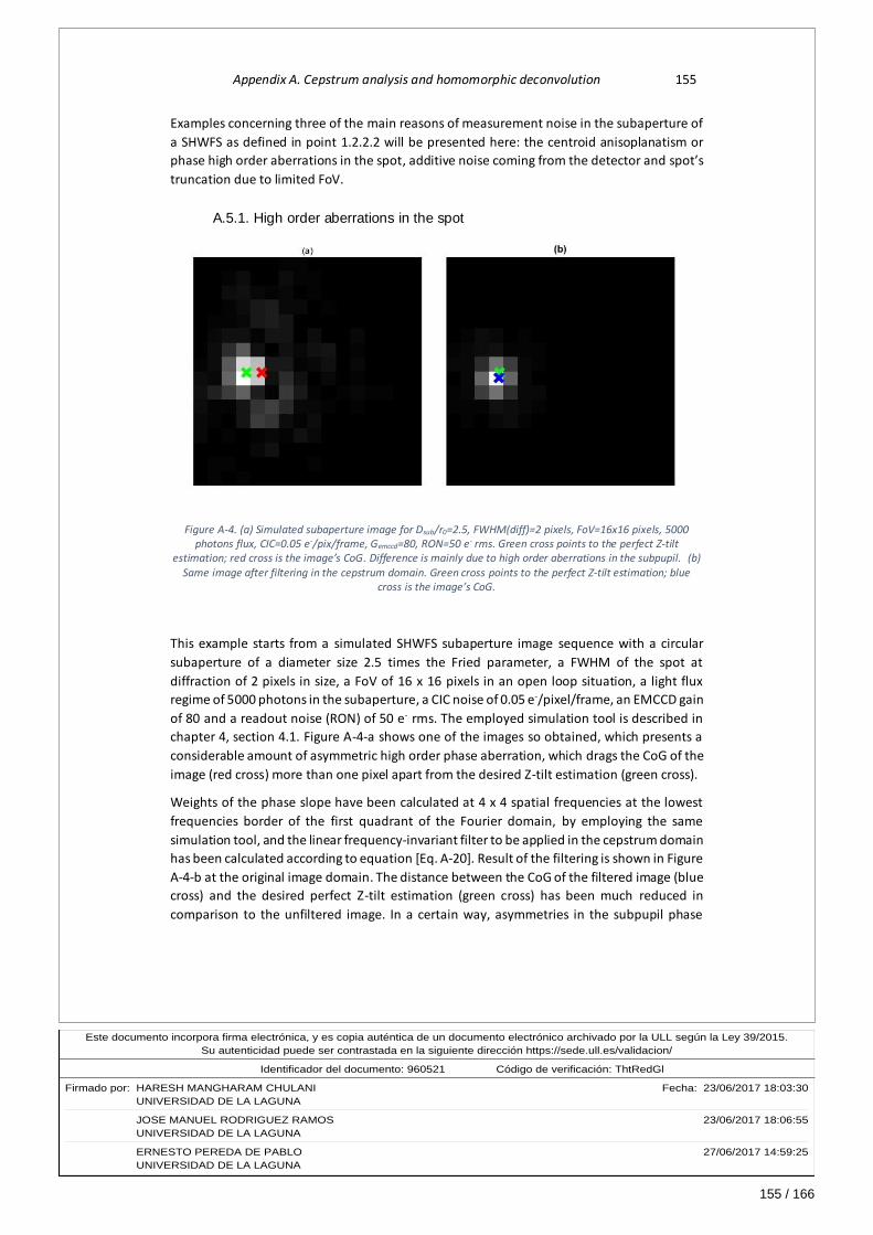
155 / 166
Este documento incorpora firma electrónica, y es copia auténtica de un documento electrónico archivado por la ULL según la Ley 39/2015.Su autenticidad puede ser contrastada en la siguiente dirección https://sede.ull.es/validacion/
Identificador del documento: 960521Código de verificación: ThtRedGl
Firmado por: HARESH MANGHARAM CHULANI Fecha: 23/06/2017 18:03:30UNIVERSIDAD DE LA LAGUNA
JOSE MANUEL RODRIGUEZ RAMOS 23/06/2017 18:06:55UNIVERSIDAD DE LA LAGUNA
ERNESTO PEREDA DE PABLO 27/06/2017 14:59:25UNIVERSIDAD DE LA LAGUNA
Appendix A. Cepstrum analysis and homomorphic deconvolution 155
Examples concerning three of the main reasons of measurement noise in the subaperture of
a SHWFS as defined in point 1.2.2.2 will be presented here: the centroid anisoplanatism or
phase high order aberrations in the spot, additive noise coming from the detector and spot’s
truncation due to limited FoV.
A.5.1. High order aberrations in the spot
This example starts from a simulated SHWFS subaperture image sequence with a circular
subaperture of a diameter size 2.5 times the Fried parameter, a FWHM of the spot at
diffraction of 2 pixels in size, a FoV of 16 x 16 pixels in an open loop situation, a light flux
regime of 5000 photons in the subaperture, a CIC noise of 0.05 e-/pixel/frame, an EMCCD gain
of 80 and a readout noise (RON) of 50 e- rms. The employed simulation tool is described in
chapter 4, section 4.1. Figure A-4-a shows one of the images so obtained, which presents a
considerable amount of asymmetric high order phase aberration, which drags the CoG of the
image (red cross) more than one pixel apart from the desired Z-tilt estimation (green cross).
Weights of the phase slope have been calculated at 4 x 4 spatial frequencies at the lowest
frequencies border of the first quadrant of the Fourier domain, by employing the same
simulation tool, and the linear frequency-invariant filter to be applied in the cepstrum domain
has been calculated according to equation [Eq. A-20]. Result of the filtering is shown in Figure
A-4-b at the original image domain. The distance between the CoG of the filtered image (blue
cross) and the desired perfect Z-tilt estimation (green cross) has been much reduced in
comparison to the unfiltered image. In a certain way, asymmetries in the subpupil phase
Figure A-4. (a) Simulated subaperture image for Dsub/r0=2.5, FWHM(diff)=2 pixels, FoV=16x16 pixels, 5000 photons flux, CIC=0.05 e-/pix/frame, Gemccd=80, RON=50 e- rms. Green cross points to the perfect Z-tilt
estimation; red cross is the image’s CoG. Difference is mainly due to high order aberrations in the subpupil. (b) Same image after filtering in the cepstrum domain. Green cross points to the perfect Z-tilt estimation; blue
cross is the image’s CoG.

156 / 166
Este documento incorpora firma electrónica, y es copia auténtica de un documento electrónico archivado por la ULL según la Ley 39/2015.Su autenticidad puede ser contrastada en la siguiente dirección https://sede.ull.es/validacion/
Identificador del documento: 960521Código de verificación: ThtRedGl
Firmado por: HARESH MANGHARAM CHULANI Fecha: 23/06/2017 18:03:30UNIVERSIDAD DE LA LAGUNA
JOSE MANUEL RODRIGUEZ RAMOS 23/06/2017 18:06:55UNIVERSIDAD DE LA LAGUNA
ERNESTO PEREDA DE PABLO 27/06/2017 14:59:25UNIVERSIDAD DE LA LAGUNA
156 Weighted Fourier Phase Slope
which are not very pronounced will derive in a non-symmetrical diffused “tail” in the spot.
This “tail” resembles a set of echoes or reverberation of the main spot and can be adequately
dealt with by cepstrum deconvolution.
A.5.2. Low light flux level
This second example starts from a simulated SHWFS subaperture image sequence with a
circular subaperture of a diameter size 2.5 times the Fried parameter, a FWHM of the spot at
diffraction of 2 pixels in size, a FoV of 16 x 16 pixels in an open loop situation, a light flux
regime of 50 photons in the subaperture, a CIC noise of 0.05 e-/pixel/frame, an EMCCD gain
of 1000 and a readout noise (RON) of 50 e- rms. Figure A-5-a shows one of the images so
obtained, which shows a spot near a corner of the FoV and spurious CIC noise randomly
distributed across the FoV, with a considerable portion far apart from the spot. Thus, the CoG
of the image is dragged towards its centre (red cross), at around 3 pixels of distance from the
desired Z-tilt estimation (green cross).
A 3 x 3 set of weights has been calculated for each axis of the Fourier phase slope, and the
frequency-invariant linear filter obtained through equation [Eq. A-20]. Result of the cepstrum
filtering as reflected in the original image domain is shown in Figure A-5-b. The CoG of the
filtered image (blue cross) is almost over the centre of the most luminous pixel, very much
closer to the desired Z-tilt estimation (green cross) than before filtering. Spurious charge noise
very much resembles echoes of the main spot, and can be tackled successfully by cepstrum
low pass frequency-invariant filtering.
Figure A-5. (a) Simulated subaperture image for Dsub/r0=2.5, FWHM(diff)=2 pixels, FoV=16x16 pixels, 50 photons flux, CIC=0.05 e-/pix/frame, Gemccd=1000, RON=50 e- rms. Green cross points to the perfect Z-tilt
estimation; red cross is the image’s CoG. Difference is mainly due to spurious charge noise in a large FoV. (b)
Same image after filtering in the cepstrum domain. Green cross points to the perfect Z-tilt estimation; blue cross is the image’s CoG.
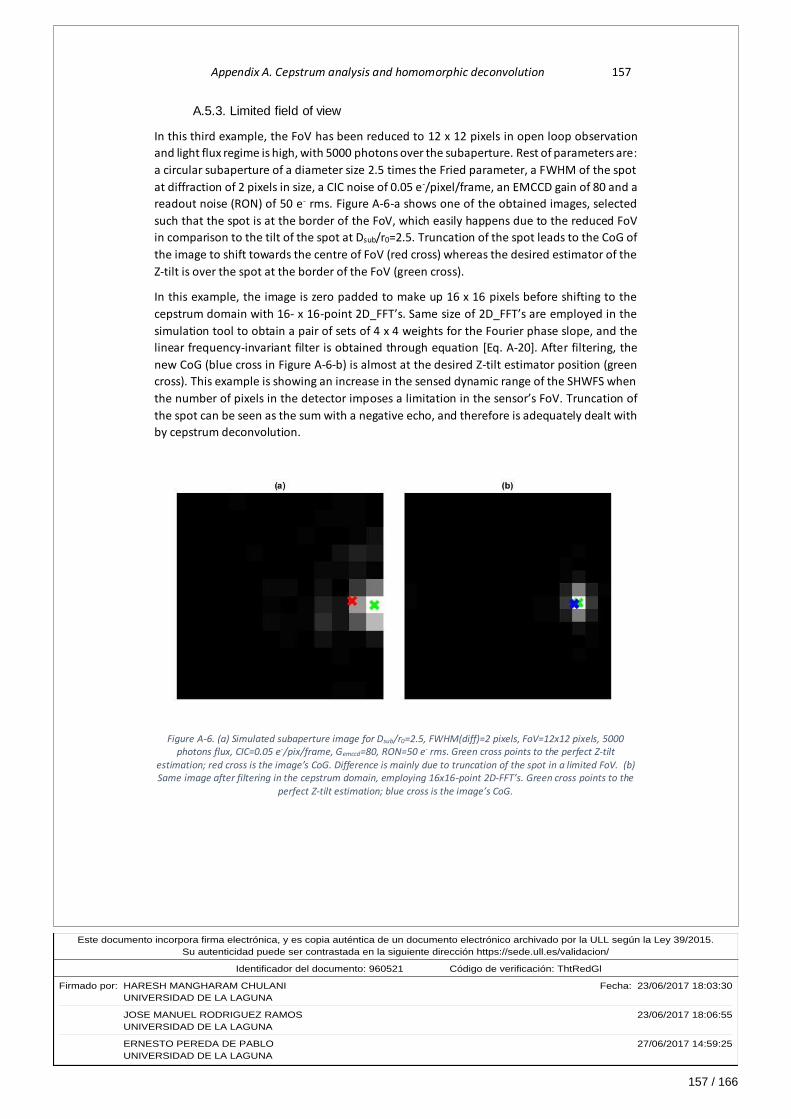
157 / 166
Este documento incorpora firma electrónica, y es copia auténtica de un documento electrónico archivado por la ULL según la Ley 39/2015.Su autenticidad puede ser contrastada en la siguiente dirección https://sede.ull.es/validacion/
Identificador del documento: 960521Código de verificación: ThtRedGl
Firmado por: HARESH MANGHARAM CHULANI Fecha: 23/06/2017 18:03:30UNIVERSIDAD DE LA LAGUNA
JOSE MANUEL RODRIGUEZ RAMOS 23/06/2017 18:06:55UNIVERSIDAD DE LA LAGUNA
ERNESTO PEREDA DE PABLO 27/06/2017 14:59:25UNIVERSIDAD DE LA LAGUNA
Appendix A. Cepstrum analysis and homomorphic deconvolution 157
A.5.3. Limited field of view
In this third example, the FoV has been reduced to 12 x 12 pixels in open loop observation
and light flux regime is high, with 5000 photons over the subaperture. Rest of parameters are:
a circular subaperture of a diameter size 2.5 times the Fried parameter, a FWHM of the spot
at diffraction of 2 pixels in size, a CIC noise of 0.05 e-/pixel/frame, an EMCCD gain of 80 and a
readout noise (RON) of 50 e- rms. Figure A-6-a shows one of the obtained images, selected
such that the spot is at the border of the FoV, which easily happens due to the reduced FoV
in comparison to the tilt of the spot at Dsub/r0=2.5. Truncation of the spot leads to the CoG of
the image to shift towards the centre of FoV (red cross) whereas the desired estimator of the
Z-tilt is over the spot at the border of the FoV (green cross).
In this example, the image is zero padded to make up 16 x 16 pixels before shifting to the
cepstrum domain with 16- x 16-point 2D_FFT’s. Same size of 2D_FFT’s are employed in the
simulation tool to obtain a pair of sets of 4 x 4 weights for the Fourier phase slope, and the
linear frequency-invariant filter is obtained through equation [Eq. A-20]. After filtering, the
new CoG (blue cross in Figure A-6-b) is almost at the desired Z-tilt estimator position (green
cross). This example is showing an increase in the sensed dynamic range of the SHWFS when
the number of pixels in the detector imposes a limitation in the sensor’s FoV. Truncation of
the spot can be seen as the sum with a negative echo, and therefore is adequately dealt with
by cepstrum deconvolution.
Figure A-6. (a) Simulated subaperture image for Dsub/r0=2.5, FWHM(diff)=2 pixels, FoV=12x12 pixels, 5000 photons flux, CIC=0.05 e-/pix/frame, Gemccd=80, RON=50 e- rms. Green cross points to the perfect Z-tilt
estimation; red cross is the image’s CoG. Difference is mainly due to truncation of the spot in a limited FoV. (b) Same image after filtering in the cepstrum domain, employing 16x16-point 2D-FFT’s. Green cross points to the
perfect Z-tilt estimation; blue cross is the image’s CoG.

158 / 166
Este documento incorpora firma electrónica, y es copia auténtica de un documento electrónico archivado por la ULL según la Ley 39/2015.Su autenticidad puede ser contrastada en la siguiente dirección https://sede.ull.es/validacion/
Identificador del documento: 960521Código de verificación: ThtRedGl
Firmado por: HARESH MANGHARAM CHULANI Fecha: 23/06/2017 18:03:30UNIVERSIDAD DE LA LAGUNA
JOSE MANUEL RODRIGUEZ RAMOS 23/06/2017 18:06:55UNIVERSIDAD DE LA LAGUNA
ERNESTO PEREDA DE PABLO 27/06/2017 14:59:25UNIVERSIDAD DE LA LAGUNA

159 / 166
Este documento incorpora firma electrónica, y es copia auténtica de un documento electrónico archivado por la ULL según la Ley 39/2015.Su autenticidad puede ser contrastada en la siguiente dirección https://sede.ull.es/validacion/
Identificador del documento: 960521Código de verificación: ThtRedGl
Firmado por: HARESH MANGHARAM CHULANI Fecha: 23/06/2017 18:03:30UNIVERSIDAD DE LA LAGUNA
JOSE MANUEL RODRIGUEZ RAMOS 23/06/2017 18:06:55UNIVERSIDAD DE LA LAGUNA
ERNESTO PEREDA DE PABLO 27/06/2017 14:59:25UNIVERSIDAD DE LA LAGUNA
Appendix B. Characterization of EDiFiSE’s EMCCD camera
The gain and noise model of the EMCCD (Electronic Multiplying Charge Coupled Device)
detector has been taken from Hirsch et al, 2013, and explained in point 4.1.3. This model has
been utilized in the simulations at subpupil level shown in chapter 4, and in those at the entire
pupil level shown in chapter 5. When tuning by simulations the WFPS algorithm to be used in
a real AO system, as it was done in chapter 6, and this applies to any other algorithm too, it is
important to properly model the real EMCCD detector that is going to create the SHWFS
images. This means, a proper estimation of its quantum efficiency q, Clock Induced Charge
(CIC) noise c, EMCCD gain g, Read Out Noise (RON) r, and sensitivity f. The purpose of the
present appendix is to explain how these parameters have been estimated in the context of
the present work. This characterization has been done over the EDiFiSE’s Andor iXon 860
detector with serial number X-4131.
The quantum efficiency q value has been taken from the detector’s manufacturer
specifications, in the same way as it was done in the work reported at Hirsch et al, 2013.
Concretely, the value 0.97 or 97% has been employed throughout this work, which is the value
at the peak of the quantum efficiency curve and a good approximation for the wavelength
range from ~500 to ~650 nm. This means that the assumption has been made in the
simulations throughout this work that the sensing wavelength is somewhere in the
mentioned range. It also means that, when incident photons have been estimated in chapter
6, again the simplifying assumption of the light being concentrated in this wavelength range
was made.
For the sensitivity estimation, the mean-variance method is proposed at Hirsch’s paper, which
can be expressed as:
𝑓 = �̅�𝑖𝑐/𝜎𝑛𝑖𝑐2 [Eq. B-1]
with �̅�𝑖𝑐 the mean of image counts level and 𝜎𝑛𝑖𝑐2 its variance. Here, the assumptions are made
that the EMCCD gain is turned off and that the image counts variance is dominated by Poisson
distributed noise. This implies a high light level, well above RON, and a well stabilized light

160 / 166
Este documento incorpora firma electrónica, y es copia auténtica de un documento electrónico archivado por la ULL según la Ley 39/2015.Su autenticidad puede ser contrastada en la siguiente dirección https://sede.ull.es/validacion/
Identificador del documento: 960521Código de verificación: ThtRedGl
Firmado por: HARESH MANGHARAM CHULANI Fecha: 23/06/2017 18:03:30UNIVERSIDAD DE LA LAGUNA
JOSE MANUEL RODRIGUEZ RAMOS 23/06/2017 18:06:55UNIVERSIDAD DE LA LAGUNA
ERNESTO PEREDA DE PABLO 27/06/2017 14:59:25UNIVERSIDAD DE LA LAGUNA
160 Weighted Fourier Phase Slope
source. This last condition was not met in the present work’s case, because the
characterization was made in-situ, in the same setup described in point 6.2.1, and not in any
specifically designed characterization setup. A workaround was therefore needed, and this is
explained in the following paragraphs.
As for the EMCCD gain, a similar mean-variance method is proposed again at Hirsch’s paper,
according to the following expression:
𝑔 = 𝑓𝜎𝑛𝑖𝑐𝑔2
2�̅�𝑖𝑐𝑔 [Eq. B-2]
where the superscript g has been added to �̅�𝑖𝑐 just to indicate that the image counts are
obtained with the EMCCD gain applied. Here again the assumption is made that Poisson noise
dominates, which is easily achieved when applying a moderate gain. Also, by applying the
gain, acquired image sequences will span a much shorter time period than for the sensitivity
estimation for the same final light level, and hence stability of the light source for such shorter
periods is easily achieved. The factor of 2 in the denominator of [Eq. B-2] is the so called Excess
Noise Factor (ENF), which has been seen to be of this value for gains over 100 (Robbins and
Hadwen, 2003), and is a consequence of the Electronic Multiplication stochastic process.
Another method to estimate the EMCCD gain could simply be to compute the ratio of light
levels with and without applied gain:
𝑔 =�̅�𝑖𝑐𝑔
�̅�𝑖𝑐 [Eq. B-3]
In this case, any offset applied by the electronics of the detector should be subtracted from
the measured signal. This second method of gain estimation has the advantage to be
independent of sensitivity estimation. In the present work, the method in equation [Eq. B-3]
has been utilized first, and then the method in equation [Eq. B-2] has been employed to
estimate the sensitivity value, by equalling the estimated gains obtained by both methods.
This has been done for five values of programmed EMCCD gains and with the detector cooled
at -80ºC. The measured gains and sensitivity values obtained thereof are listed in Table B-1.
Programmed Gemccd Measured Gemccd Sensitivity f in e-/ADU
10 8.6 16.35 100 80.63 15.72 300 226.10 15.47 500 385.99 16.08 1000 860.15 17.80
Table B-1. Measured EMCCD gains vs. programmed gains, and sensitivity values obtained thereof.
It is necessary for the estimation of the detector noises to have an estimated sensitivity value,
as will be seen further on. A sensitivity value of 16 e-/ADU has been selected. As for the
EMCCD gain, the value obtained by equation [Eq. B-2] with the mentioned sensitivity of 16
will be taken as the estimated gain.

161 / 166
Este documento incorpora firma electrónica, y es copia auténtica de un documento electrónico archivado por la ULL según la Ley 39/2015.Su autenticidad puede ser contrastada en la siguiente dirección https://sede.ull.es/validacion/
Identificador del documento: 960521Código de verificación: ThtRedGl
Firmado por: HARESH MANGHARAM CHULANI Fecha: 23/06/2017 18:03:30UNIVERSIDAD DE LA LAGUNA
JOSE MANUEL RODRIGUEZ RAMOS 23/06/2017 18:06:55UNIVERSIDAD DE LA LAGUNA
ERNESTO PEREDA DE PABLO 27/06/2017 14:59:25UNIVERSIDAD DE LA LAGUNA
Appendix B. Characterization of EDiFiSE’s EMCCD camera 161
Till now, the sensitivity and gain parameters have been estimated from illuminated images.
Noise parameters need to be estimated from dark images. In Hirsch et al, 2013, the employed
estimation method for the noise parameters is the Maximum Likelihood (ML) method, or
maximization of the log-likelihood function, given the observation of a series of dark images
and assuming a concrete parametric model for dark images, with c, g, r and f as the
parameters, and with a Poisson, a gamma and a normal components, as explained in point
4.1.3. The sensitivity f and the gain g are obtained by mean-variance methods over
illuminated images (equations [Eq. B-1] and [Eq. B-2], respectively). Read out noise r and CIC
noise c are determined jointly by maximization of the mentioned likelihood function.
In the present work, noises are estimated by minimization of the difference between the
observed histogram of a dark image sequence and the histogram obtained from the
parametric model proposed in Hirsch’s work. The difference with the mentioned work is that
only one parameter is estimated, which is the bias offset at the dark image, and the r and c
noise components are obtained as a function of the observed values and the estimated offset.
This is done on a pixel by pixel basis over a selection of random pixels throughout the whole
image, and final values are obtained by averages among all evaluated pixels. This method was
validated by characterizing other detectors from the same manufacturer, in a work by a
student at the IAC and co-tutored by the author (Pinna F., 2014).
After offset subtraction in an observed dark image, negative image counts are due to negative
normal RON exclusively. Therefore, r in rms electron units can be estimated from such
negative image counts as:
�̂� = 𝑓[(𝑛𝑖𝑐 − 𝑜𝑓𝑓𝑠𝑒𝑡)2̅̅ ̅̅ ̅̅ ̅̅ ̅̅ ̅̅ ̅̅ ̅̅ ̅̅ ̅̅ ]1/2,, 𝑛𝑖𝑐 < 𝑜𝑓𝑓𝑠𝑒𝑡 [Eq. B-4]
Whereas CIC noise is the reason for a positive mean in the observed dark image18, and can
therefore be estimated in electron units as:
�̂� = (�̅�𝑖𝑐 − 𝑜𝑓𝑓𝑠𝑒𝑡)𝑓/𝑔 [Eq. B-5]
Finally, the electronic offset is estimated by the minimization of the distance between the
probability density function (PDF) obtained from the observed dark image counts and the one
obtained from the model at Hirsch’s work:
휀𝑝 = ∫|𝑝(𝑛𝑖𝑐 ;𝑜𝑏𝑠𝑒𝑟𝑣𝑒𝑑) − 𝑝(𝑛𝑖𝑐 ;𝑞, 𝑐, 𝑔, 𝑟, 𝑓, 𝑜𝑓𝑓𝑠𝑒𝑡)|𝑑𝑝 [Eq. B-6]
𝑝(𝑛𝑖𝑐; 𝑜𝑏𝑠𝑒𝑟𝑣𝑒𝑑) is the PDF which depends only on the observed values in the dark image,
and 𝑝(𝑛𝑖𝑐 ;𝑞, 𝑐, 𝑔, 𝑟, 𝑓, 𝑜𝑓𝑓𝑠𝑒𝑡) is the parametric model from Hirsch’s paper with an offset
added. q, g and f are determined as previously explained. c and r are estimated by equations
[Eq. B-5] and [Eq. B-4], respectively. And so, the only left parameter to estimate is the offset,
18 Dark images were taken with the detector’s shutter off.

162 / 166
Este documento incorpora firma electrónica, y es copia auténtica de un documento electrónico archivado por la ULL según la Ley 39/2015.Su autenticidad puede ser contrastada en la siguiente dirección https://sede.ull.es/validacion/
Identificador del documento: 960521Código de verificación: ThtRedGl
Firmado por: HARESH MANGHARAM CHULANI Fecha: 23/06/2017 18:03:30UNIVERSIDAD DE LA LAGUNA
JOSE MANUEL RODRIGUEZ RAMOS 23/06/2017 18:06:55UNIVERSIDAD DE LA LAGUNA
ERNESTO PEREDA DE PABLO 27/06/2017 14:59:25UNIVERSIDAD DE LA LAGUNA
162 Weighted Fourier Phase Slope
and this is accomplished by minimizing 휀𝑝. By multiplying 휀𝑝 by 100, a histogram relative
fitting error in percentage units is obtained.
Figure B-1. Histograms of dark images for a situation without EMCCD gain. Blue trace is for a real acquired signal from a single pixel of EDiFiSE’s SHWFS detector. Green trace is for a simulated signal following the
EMCCD model described in Hirsch et al, 2013.
Figure B-2. Histograms of dark images for a situation with programmed EMCCD gain of 100. Blue trace is for a
real acquired signal from a single pixel of EDiFiSE’s SHWFS detector. Green trace is for a simulated signal following the EMCCD model described in Hirsch et al, 2013.

163 / 166
Este documento incorpora firma electrónica, y es copia auténtica de un documento electrónico archivado por la ULL según la Ley 39/2015.Su autenticidad puede ser contrastada en la siguiente dirección https://sede.ull.es/validacion/
Identificador del documento: 960521Código de verificación: ThtRedGl
Firmado por: HARESH MANGHARAM CHULANI Fecha: 23/06/2017 18:03:30UNIVERSIDAD DE LA LAGUNA
JOSE MANUEL RODRIGUEZ RAMOS 23/06/2017 18:06:55UNIVERSIDAD DE LA LAGUNA
ERNESTO PEREDA DE PABLO 27/06/2017 14:59:25UNIVERSIDAD DE LA LAGUNA
Appendix B. Characterization of EDiFiSE’s EMCCD camera 163
Figure B-3. Histograms of dark images for a situation with programmed EMCCD gain of 300. Blue trace is for a real acquired signal from a single pixel of EDiFiSE’s SHWFS detector. Green trace is for a simulated signal
following the EMCCD model described in Hirsch et al, 2013.
Figure B-4. Histograms of dark images for a situation with programmed EMCCD gain of 500. Blue trace is for a real acquired signal from a single pixel of EDiFiSE’s SHWFS detector. Green trace is for a simulated signal
following the EMCCD model described in Hirsch et al, 2013.
Figures B-1 to B-5 show the results of a dark image histogram fitting for a single pixel and
programmed EMCCD gains of 1 (no gain), 100, 300, 500 and 1000. Blue traces are for the
observed image counts, and green traces are from the parametric model. It is interesting to
see how, for the tails due to CIC noise, the model always gives less occurrences for lower

164 / 166
Este documento incorpora firma electrónica, y es copia auténtica de un documento electrónico archivado por la ULL según la Ley 39/2015.Su autenticidad puede ser contrastada en la siguiente dirección https://sede.ull.es/validacion/
Identificador del documento: 960521Código de verificación: ThtRedGl
Firmado por: HARESH MANGHARAM CHULANI Fecha: 23/06/2017 18:03:30UNIVERSIDAD DE LA LAGUNA
JOSE MANUEL RODRIGUEZ RAMOS 23/06/2017 18:06:55UNIVERSIDAD DE LA LAGUNA
ERNESTO PEREDA DE PABLO 27/06/2017 14:59:25UNIVERSIDAD DE LA LAGUNA
164 Weighted Fourier Phase Slope
image counts and more occurrences for higher image counts. This is quite probably because
the model assumes that CIC noise is only produced in the charge transfers before the EM
register, whereas actually some CIC noise is produced in the EM register itself and is affected
by lower EMCCD gains than the total gain.
Figure B-5. Histograms of dark images for a situation with programmed EMCCD gain of 1000. Blue trace is for a real acquired signal from a single pixel of EDiFiSE’s SHWFS detector. Green trace is for a simulated signal
following the EMCCD model described in Hirsch et al, 2013.
Programmed Gemccd
Estimated
Gemccd CIC (e-)
RON (rms e-)
Estimated
offset
εp (%)
1 1 0 47.36 100.7 3.77 100 82.04 0.156 48.08 98.8 4.66 300 233.92 0.144 48.77 97.7 4.22 500 384.07 0.158 52.18 96.9 5.64 1000 773.43 0.161 62.55 94.0 8.87
Table B-2. Estimated offset and subsequent CIC and RON values obtained by dark images histogram fitting for the listed programmed EMCCD gains.
Table B-2 collects the results for offset, CIC and RON estimation from the previous figures.
Also, the gains introduced in the parametric model are listed, as well as the final histogram
fitting error.
Finally, a good approximation for the parameters introduced in the model of EDiFiSE’s SHWFS
detector have been: a sensitivity of 16 e-/ADU; a gain which is 20% less than the programmed
one, i.e., 160 for a programmed gain of 200, and 800 for a programmed 1000 gain; a CIC noise
of 0.155 e-/pixel/frame; a RON of 50 rms e-; and a QE of 97%.

165 / 166
Este documento incorpora firma electrónica, y es copia auténtica de un documento electrónico archivado por la ULL según la Ley 39/2015.Su autenticidad puede ser contrastada en la siguiente dirección https://sede.ull.es/validacion/
Identificador del documento: 960521Código de verificación: ThtRedGl
Firmado por: HARESH MANGHARAM CHULANI Fecha: 23/06/2017 18:03:30UNIVERSIDAD DE LA LAGUNA
JOSE MANUEL RODRIGUEZ RAMOS 23/06/2017 18:06:55UNIVERSIDAD DE LA LAGUNA
ERNESTO PEREDA DE PABLO 27/06/2017 14:59:25UNIVERSIDAD DE LA LAGUNA

166 / 166
Este documento incorpora firma electrónica, y es copia auténtica de un documento electrónico archivado por la ULL según la Ley 39/2015.Su autenticidad puede ser contrastada en la siguiente dirección https://sede.ull.es/validacion/
Identificador del documento: 960521Código de verificación: ThtRedGl
Firmado por: HARESH MANGHARAM CHULANI Fecha: 23/06/2017 18:03:30UNIVERSIDAD DE LA LAGUNA
JOSE MANUEL RODRIGUEZ RAMOS 23/06/2017 18:06:55UNIVERSIDAD DE LA LAGUNA
ERNESTO PEREDA DE PABLO 27/06/2017 14:59:25UNIVERSIDAD DE LA LAGUNA