1

Configurable Architectures for Multi-Mode Floating

Point AddersManish Kumar Jaiswal, B. Sharat Chandra Varma, Hayden K.-H. So, M. Balakrishnan, Kolin Paul and

Ray C.C. Cheung

Abstract—This paper presents two architectures for floatingpoint (F.P.) adders, which operates in multi-mode configurationwith multi-precision support. First architecture (named QPdDP)works in dual-mode which can operates either for quadrupleprecision or two-parallel double precision. The second architec-ture (named QPdDPqSP) works in tri-mode which is able tocompute either of a quadruple precision, two-parallel doubleprecision and four-parallel single precision computations. Thearchitectures are based on the standard state-of-the-art flowfor F.P. adder which supports the computation of normal andsub-normal operands, along with the support for the excep-tional case handling. The key components in the architecture,such as comparator, swap, dynamic shifters, leading-one-detector(LOD), mantissa adders/subtractors, and rounding circuit, arere-designed & optimized for multi-mode computation, to enableefficient resource sharing for multi-precision operands. The data-path in each multi-mode architecture is tuned for multi-precisionsupport with minimal multiplexing circuitry overhead. Theseproposed architectures provide multi-precision SIMD supportfor lower precision operands, along with high precision computa-tional support, and thus, have a better resource utilization. A fullypipelined version of both adder architectures are presented. Theproposed adder architectures are synthesized using UMC 90nmtechnology ASIC implementation. The proposed architecturesare compared with the best available literature works, andhave shown better design metrics in terms of area, delay andarea× period, along with more computational support.

Keywords-Floating Point Addition, Multi-Mode Multi-precisionArithmetic, SIMD, ASIC, Digital Arithmetic, Configurable Ar-chitecture.

I. INTRODUCTION

Floating point (FP) number system [1], due to its wide

dynamic range, is a common choice for a large set of scientific,

engineering and numerical processing computations. Gener-

ally, the performance of these computations greatly depends on

the underlying floating point arithmetic processing unit. Sev-

eral contemporary general purpose processors provide SIMD

support for parallel floating point arithmetic computation. This

Copyright (c) 2015 IEEE. Personal use of this material is permitted.However, permission to use this material for any other purposes must beobtained from the IEEE by sending an email to pubs-permissions@ieee.org.

This work is party supported by the The University of Hong Kong grant(Project Code. 201409176200), the Research Grants Council of Hong Kong(Project ECS 720012E), and the Croucher Innovation Award 2013.

Manish Kumar Jaiswal, B. Sharat Chandra Varma, Hayden K.-H. So arewith Department of EEE, The University of Hong Kong, Hong Kong e-mail:{manishkj,varma,hso}@eee.hku.hk

M. Balakrishnan and Kolin Paul are with Department of CSE, IndianInstitute of Technology, Delhi, India. e-mail: {mbala,kolin}@cse.iitd.ernet.in

Ray C.C. Cheung is with Department of EE, City University of Hong Kong,Hong Kong e-mail: r.cheung@cityu.edu.hk

is achieved by using multiple units of single precision and

double precision arithmetic hardware.

To provide much higher floating point computational sup-

port, several custom high performance computing machines

from major semiconductor companies like Intel, IBM, ARM,

and Nvidia, provide huge multi-core computing systems. Each

core in these generally contains a larger vector floating point

unit (VFU). The VFU units in these computing system cores

contain separate vector processing arrays of single precision

and double precision computational units. Like, the Synergistic

Processing Element (SPE), in Cell-BE processor [2] from

IBM, contains a vector array of 4 single precision and an

array of 2 double precision. The ARM VFU co-processor

(VFU9-S) [3] provides a vector array of 16 single precision FP

units and 8 double precision vector array. Like wise, the Intel

has developed a 60 core Xeon PhiTM computing machine,

in which each core contains an array of 16 single precision

units and an array of 8 double precision units. Similarly, the

Nvidia’s next generation CUDATM architecture: KeplerTM

GK110 [4] contains 15 Streaming Multiprocessor (SMX), in

which each SMX contains 192 single precision core and 64

double precision core. Generally, these processing systems

contain separate units/arrays for single precision and double

precision computations. However, if an unified dynamically

configurable computational unit can support a double precision

with dual/two-parallel single precision (DPdSP) arithmetic, or

quadruple precision with dual/two-parallel double precision

(QPdDP) arithmetic, it can save a large silicon area in the

above computing machines.

Furthermore, the availability for double precision arithmetic

computation is not enough and the demand for high precision

arithmetic is increasing in many application areas [5], [6]. In

this view, this paper is aimed towards the configurable multi-

mode multi-precision floating arithmetic architecture design,

currently aiming towards the addition/subtraction arithmetic,

with high precision support.

Some literature have focused on the standard cell based

ASIC architectures for configurable dual-mode multi-precision

floating point arithmetic, included with quadruple precision

support [7]–[17]. Many of these works [7]–[11] are dedicated

to the dual-mode multiplier design, and [12] proposed a dual-

mode FMA architecture. Isseven et al. [14] proposed a dual-

mode division architecture. Some literature [15]–[17] have

proposed dual-mode architectures for adder. These works have

tried to improve the resource utilization for the hardware with

multi-precision computational support. However, the overhead

of extra hardware, and un-optimized data-path and resource

2

sharing lead to large overhead of area and delay metrics. Fur-

thermore, they have limited support only for normal operands.

The dual-mode adder architectures of [15], [16] used a large

number of multiplexers (to support dual mode) at various

level of architecture, and have less tuned data path for dual

mode operation. Further the extra use of resources (like more

adders/subtractors for exponent & mantissa, relatively larger

dual shifters, extra mantissa normalizing shifters for dual mode

support) made their area & delay overhead larger. Some recent

literature by [18], [19] have also worked on the dual-mode

DPdSP addition and division architectures.

This work is built on top of the work proposed by Jaiswal et

al. [18] for dual-mode DPdSP adder architecture. This paper

is extending the idea of dual-mode DPdSP adder architecture

to the dual-mode QPdDP (quadruple precision with dual/two-

parallel double precision) adder architecture. Furthermore, this

paper also proposes a new tri-mode QPdDPqSP (quadruple

precision with dual/two-parallel with quad/four-parallel single

precision) adder architecture. The tri-mode adder architecture

is a fresh proposal. The computational components of the float-

ing point adder arithmetic are constructed for the on-the-fly

or configurable multi-mode multi-precision support. The data-

path is tuned for better resource sharing and to minimize the

multiplexing circuitry. All the proposed architectures are pro-

vided with the full supports for normal as well as sub-normal

operands computation, exceptional case handling, and with

round-to-nearest rounding method. Other rounding methods

can also be easily included. Both architectures are designed

with 4-stage pipeline and synthesized for a 90nm standard cell

based ASIC implementation. The proposed architectures are

compared with the best optimized implementations available

in the literature. The main contributions of this work can be

summarized as follows:

• A dual-mode QPdDP adder architecture is proposed

which can process either a Quadruple Precision or dual

(two parallel) Double Precision addition/subtraction. An

architecture for tri-mode QPdDPqSP adder is also pro-

posed, which can process either a Quadruple Precision

or dual (two parallel) Double Precision or quad (four

parallel) Single Precision additions/subtractions.

• Both proposed architectures provide high precision com-

putational support as well as SIMD support for the lower

precision computations.

• The architectural sub-components and data-path are con-

structed for the configurable multi-mode operation, which

enables efficient resource utilization with multi-precision

support.

• The proposed dual-mode QPdDP architecture has smaller

area × period metric in comparison with the best

available literature. Moreover, the proposal on tri-mode

QPdDPqSP architecture also shows a promising design

metrics, and stand as a fresh contribution on tri-mode

adder architecture.

This manuscript is organized as follows. Section II briefly

discusses the basic algorithmic flow of the floating point

adder arithmetic, which is used in current context for multi-

mode processing. Section III describes the proposed dual-

mode QPdDP adder architecture and section IV discusses the

proposed tri-mode QPdDPqSP adder architecture. The detail

implementation results and related comparisons with previous

literature work are presented in the section V. Finally, the

manuscript is concluded in section VI.

II. BACKGROUND

The present work on the multi-mode floating point adder

architecture follows the basic single-path algorithm for this

computation. A floating point arithmetic computation involves

computing separately the sign, exponent and mantissa part

of the operands, and later combine them after rounding and

normalization [1]. The standard format for floating point

numbers are as follows:

SP :

Sign︷ ︸︸ ︷

1− bit

Exponent︷ ︸︸ ︷

8− bit

Mantissa︷ ︸︸ ︷

23− bit

DP :

Sign︷ ︸︸ ︷

1− bit

Exponent︷ ︸︸ ︷

11− bit

Mantissa︷ ︸︸ ︷

52− bit

QP :

Sign︷ ︸︸ ︷

1− bit

Exponent︷ ︸︸ ︷

15− bit

Mantissa︷ ︸︸ ︷

112− bit

A basic state-of-the-art computational flow of the floating

point adder is shown in the Algorithm 1. Here, steps 6-7 and

step-22 require for sub-normal processing. Sub-normals repre-

sents the numbers whose magnitude fall beyond the minimum

normal format value. The sub-normal representation helps in

preserving the underflown result of a computation, which can

not be represented by a valid normal number. The unification

of these normal and sub-normal number in floating point

representation, generally, makes the floating point computation

a tough task. In present work of multi-mode multi-precision

architectures, each steps of the flow are constructed for the

support of the multi-mode operation with resource sharing and

tuned data-path with minimum multiplexing circuitry.

III. CONFIGURABLE QUADRUPLE PRECISION / DUAL

(TWO-PARALLEL) DOUBLE PRECISION (QPDDP) ADDER

ARCHITECTURE

The architecture for proposed QPdDP adder is presented

here to provide the higher precision requirements of the

applications, with dual-mode support. The computational flow

of the QPdDP adder architecture is based on the Algorithm 1

and the architecture is shown in Fig. 1. The input/output

register for this architecture is assumed as shown in Fig. 2. The

two 128-bit input operands, contain either 1 set of quadruple

precision or 2 sets of double precision operands. Based on the

mode deciding control signal (qp dp), the dual-mode archi-

tecture switched to either quadruple precision or dual (two-

parallel) double precision computation mode (qp dp: 1 → QP

Mode, qp dp: 0 → Dual DP Mode). All the computational

steps in QPdDP dual mode adder are discussed below in detail.

The data-extraction, sub-normal and exceptional handling

are shown in the Fig. 3. Based on the precision format, the

sign, exponent and mantissa parts of the operands are extracted

for both, the quadruple precision and double precision.

3

Algorithm 1 F.P. Adder Computational Flow [1]

1: (IN1, IN2) Input Operands;2: Data Extraction & Exceptional Check-up:3: {S1(Sign1), E1(Exponent1), M1(Mantissa1)} ← IN1

4: {S2, E2, M2} ← IN2

5: Check for INFINITY, NAN6: Check for SUB-NORMALs7: Update Exponents & Mantissa’s MSB for SUB-NORMALs8: COMPARE, SWAP & Dynamic Right SHIFT:9: IN1 gt IN2← {E1,M1} ≥ {E2,M2}

10: Large E,M ← IN1 gt IN2 ? E1,M1 : E2,M211: Small E,M ← IN1 gt IN2 ? E2,M2 : E1,M112: Right Shift ← Large E - Small E13: Small M ← Small M >> Right Shift14: Mantissa Computation:15: OP ← S1⊕ S216: if OP == 1 then17: Add M ← Large M + Small M18: else19: Add M ← Large M - Small M20: Leading-One-Detection & Dynamic Left SHIFT:21: Left Shift ← LOD(Add M)22: Left Shift← Adjustment for SUB-NORMAL or Underflow23: Add M ← Add M << Left Shift24: Normalization & Rounding:25: Mantissa Normalization & Compute Rounding ULP based

on Guard, Round & Sticky Bit26: Add M ← Add M + ULP27: Large E ← Large E + Add M[MSB] - Left Shift28: Finalizing Output:29: Update Exponent & Mantissa for Exceptional Cases30: Determine Final Output

As appeared in Fig. 2 that the exponent portion of QP and

second DP (DP-2) operand are overlapped.

QP Exponent︷ ︸︸ ︷

xxxxxxxxxxx︸ ︷︷ ︸

DP−2 Exponent

xxxx

This scenario is used to share the resources related to sub-

normal, infinity, and NaN detection of QP and second

DP operands. The detection of sub-normals are shown in the

Fig. 3, which detects the zero value of corresponding exponent.

Similarly, the checks for infinity and NaN are handled

(which detects the maximum binary value of corresponding

exponent). After these exceptional checks the exponent and

mantissa are updated accordingly, as shown in Fig. 3. In

comparison to only QP computation, this unit requires extra

related resources for first DP (DP-1) operands.

The dual-mode comparator unit for dual-mode QPdDP

adder is shown in Fig. 4. The comparator unit determines

which operand is large and which one is small. This unit is

shared among the QP and both DP operands. It is comprised of

two comparator units for both DPs operands, which generates

their corresponding comparison results. These DP results are

further combined to form QP comparison. The individual

‘greater-than’ and ‘equivalent’ functions are designed using

following boolean functions:

(in1 > in2) = in1n.in2n + (in1n ⊕ in2n).in1n−1.in2n−1 + . . .

. . . + (in1n ⊕ in2n) . . . (in11 ⊕ in21).in10.in20

(in1 == in2) = (in1n ⊕ in2n) . . . . . . (in10 ⊕ in20)

In terms of resources, this dual-mode comparator unit

m_L m_S e_L

Dua-Mode DRS

add_m

e_S

e_L

Data Extraction & SubNormal HandlerComparator

_sn: SubNormal-gt-: Greater than-eq-: Equal to

_L: Large_S: Small_l_: Left_r_: Right

_s: Sign_e : Exponent_m: Mantissa_op: Operation

Swap: Large Sign, Exp, Mant and OP

R_Shift_Amount

LOD_in

Left Shift Update (for subnormal, underflow)

Exponent Update (for subnormal, underflow,

overflow, exceptional cases)

Final Processing

m_ovf

m_ovf

add_mu add_ml

add_m_shifted

qp_dp

qp_dpdp1_r_shiftqp_r_shiftdp2_r_shift

qp_dpm_S_shifted

dp2_op

dp1_op

qp_opDual-Mode Add/Sub

Dual-Mode LODdp1_l_shift_tmpqp_l_shift_tmpdp2_l_shift_tmpdp1_sn

dp2_snqp_sn

qp_dp

dp2_l_shift qp_l_shift dp1_l_shiftqp_dpDual-Mode DLS

qp_dp

dp1_sndp2_sn

qp_sn

qp_dpdp1_Ls

dp2_Lsqp_Ls

qp: Quadruple Precisiondp: Double Precisionqp_dp: Quadruple/Double

Mantissa Sum & LOD_in

Normalization & Dual-Mode Rounding

in2[127:0] in1[127:0]

12812822 22

6 67

65 65

128

2128

6 67

6 67

128

128

qp_dp

128

e_L

Fig. 1: QPdDP Adder Architecture.

128-bit64-bit

15-bit 112-bit

11-bit 52-bit 11-bit 52-bit

QP[127:64] / DP2 QP[63:0] / DP1

Fig. 2: QPdDP Adder: Input / Output Register Format.

in1[62:52] in2[62:52]

dp1_sn2dp1_sn1

dp1_sn

in1[126:116] in2[126:116]

dp2_sn2dp2_sn1

dp2_sn

dp2_sn2dp2_sn1

in1[115:112] in2[115:112]

qp_sn1 qp_sn2

qp_sn

dp1_e1 = {in1[62:53], in1[52] | dp1_sn1}dp1_e2 = {in2[62:53], in2[52] | dp1_sn2}dp2_e1 = {in1[126:117], in1[116] | dp2_sn1}dp2_e2 = {in2[126:117], in2[116] | dp2_sn2}qp_e1 = {in1[126:113], in1[112] | qp_sn1}qp_e2 = {in2[126:113], in2[112] | qp_sn2}

dp1_m1 = {~dp1_sn1, in1[51:0]}dp1_m2 = {~dp1_sn2, in2[51:0]}dp2_m1 = {~dp2_sn1, in1[115:64]}dp2_m2 = {~dp2_sn2, in2[115:64]}qp_m1 = {~qp_sn1, in1[111:0]}qp_m2 = {~qp_sn2, in2[111:0]}

Sub-Normal Detection:

Exponents: Mantissas:

Fig. 3: QPdDP Adder: Data Extraction and Subnormal Han-

dler.

requires similar resources as needed in only QP comparator,

and there is no area overhead in this unit.

The next computational unit in this architecture is the Dual-

4

dp1_in1-gt-in2 = (in1[62:0] > in2[62:0]) ? 1 : 0

dp2_in1-eq-in2 = (in1[126:64] == in2[126:64]) ? 1 : 0

dp2_in1-gt-in2 = (in1[127:64] > in2[127:64]) ? 1 : 0

qp_in1-gt-in2 = dp2_in1-gt-in2 | ( dp2_in1-eq-in2 & ((in1[63]&~in2[63) | (in1[63]~^in2[63]) & dp1_in1-gt-in2) )

QP[127:64] / DP2 QP[63:0] / DP1

Compare DP-1Compare DP-2

dp2_in1-gt-in2 dp1_in1-gt-in2

qp_in1-gt-in2

DP-Comparisons:

QP-Comparison:

Fig. 4: QPdDP Adder: Comparator.

dp1_Le = e_L[10:0]dp2_Le = e_L[21:10]qp_Le = e_L[14:0]

OPdp1_op = dp1_s1 ~^ dp1_s2dp2_op = dp2_s1 ~^ dp2_s2qp_op = qp_s1 ~^ qp_s2

Large Signdp1_Ls = dp1_in1-gt-in2 ? dp1_s1 : dp1_s2dp2_Ls = dp2_in1-gt-in2 ? dp2_s1 : dp2_s2qp_Ls = qp_in1-gt-in2 ? qp_s1 : qp_s2

C1C2

e1[10:0]

e2[10:0]e_L[10:0]

e1[21:11]

e2[21:11]e_L[21:11]

Unified Large Exponent:

Unified Small Exponent: e_S[10:0] = c1 ? e2[10:0] : e1[10:0] e_S[21:11] = c2 ? e2[21:11] : e1[21:11]

Unified Large Mantissa:m_L[63:0]= c1 ? m1[63:0] : m2[63:0]m_L[127:64]= c2 ? m1[127:64] : m2[127:64]

Unified Small Mantissa:m_S[63:0]= c1 ? m2[63:0] : m1[63:0]m_S[127:64]= c2 ? m2[127:64] : m1[127:64]

0

1

0

1

Unified Exponent

qp_dp

C1

qp_dp

qp_in1_gt_in2

dp2_in1_gt_in2C2

Unified Compare

0

1qp_in1_gt_in2

dp1_in1_gt_in2 0

1

Unified Mantissa qp_dp

{qp_m1,15’b0}

m1

{dp2_m1,11’b0,dp1_m1,11’b0} 0

1

qp_dp

{qp_m2,15’b0}

m2

{dp2_m2,11’b0,dp1_m2,11’b0} 0

1

qp_dp

e1{dp2_e1,dp1_e1}

{7’b0,qp_e1}

0

1

qp_dp

e2{dp2_e2,dp1_e2}

{7’b0,qp_e2}

0

1

shift = e_L - e_S

qp_r_shift = dp_sp ? shift[14:0] : 0dp1_r_shift = ~qp_dp ? shift[10:0] : 0dp2_r_shift = ~qp_dp ? shift[21:11] :0

Right Shift Amount

Fig. 5: QPdDP Adder: SWAP - Large Sign, Exponent, Man-

tissa and OPERATION; Right Shift Amount.

Mode SWAP, which generates large sign (effectively output

sign-bit), small & large exponents, small & large mantissas

and effective operations (to be performed between large and

small mantissas). This computational unit is shown in Fig. 5.

For SWAP, in general to handle both DPs and QP, it needs four

11-bit (for both DP exponents), two 15-bit (for QP exponents),

four 53-bit (for both DP mantissas) and two 113-bit (for QP

mantissa) SWAP components for all the computations of this

section. However, to minimize the swapping overhead, the uni-

fied exponents, mantissas and greater-than control signals are

generated, by multiplexing either of the quadruple precision

or both double precision operands (as shown in Fig. 5).

This is an important step included in the dual-mode QPdDP

architectural flow, which helps to design a tuned data-path

computation in later stages, with reduced multiplexing cir-

0101

01

y=2**x

>> y

One Stage Dual-Mode Unit

[127:64] [63:0]

qp[x] | dp2[x] qp[x] | dp1[x]

[127:64] [63:0]

[63+y:64] [63-y:0]

qp_dp & qp[x]

[63:0][127:64]

>> y

in

01

Shifted Output

SHIFT<-- qp[6:0], dp2[5:0], dp1[5:0]

qp[6]

[127:0]

Dual-Mode Right Shifting (6 Stage <- f(qp[5:0], dp2[5:0], dp1[5:0])

in[127:0]<-- {[127:0]} / {[63:0],[63:0]}

in >> 64

Fig. 6: QPdDP Dual Mode Dynamic Right Shifter (DRS).

cuitry. Using these unified exponents, mantissas and greater-

than control signals, it requires only four 11-bit (for expo-

nents) and four 64-bit (for mantissas) SWAP circuitry for

entire processing. Effectively, it needs SWAP components

slightly more than it requires for only QP (only QP requires

two 15-bit SWAP for exponents and two 113-bit SWAP for

mantissas), along with extra multiplexing circuitry needed to

generate unified signals, however, facilitates the tuned data-

path processing. Further, among extra appended LSB ZEROs

in mantissa multiplexing (for m1 and m2), 3-bit are for

Guard, Round and Sticky bit computations in rounding phase,

and remaining can provide extended precision support to the

operands.

The basic functional component in SWAP unit is 2:1 MUX

(for unified data generation) and few xnor gates (for effective

operation, OP). The 2:1 MUX is implemented using simple

boolean logic as (y = sel.A + sel.B). The m L contains

mantissa of either large QP operand or both of large DP

operands. Similarly, m S contains small mantissas. Likewise,

e L contains large exponent, and e S contains small expo-

nents, either of QP or both DP operands.

Now, the small mantissa needs right shifting by the differ-

ence of large and small exponents. The right shift amount for

small mantissas are determined using the component shown in

Fig. 5. In general, it requires two 11-bit subtractors for both

double precision and one 15-bit subtractor for quadruple preci-

sion. However, because of effective multiplexing of operands

in SWAP section, it needs only one a 22-bit subtractor. A

subtraction of unified large exponent (e L) and unified small

exponent (e S) will produce right shift amount either for

quadruple precision or for both double precision. For right

shift amount, compared to only quadruple precision, it requires

extra resources for 7-bit subtraction. Other processing in this

section are bit-wise operations, and are done separately for all

operands.

For right shifting of small mantissas of quadruple and both

double precision operands, a dual-mode dynamic right shifter

(DRS) is designed. The QPdDP dual-mode dynamic right

shifter is shown in Fig. 6, which is used to right-shift the

5

add_mu add_ml

qp_dp[63:0][63:0][127:64][127:64]

qp_dpqp_opdp2_op

dp1_opqp_op

CLA Add/Sub 64-bit

add_ml[64]

CLA Add/Sub 64-bit

m_S_shiftedm_L

65 65

Fig. 7: QPdDP Adder: Dual Mode Mantissa Addi-

tion/Subtraction.

[62:0][63:0] 1

add_ml[63:1]1qp_dp

add_ml[64]

0

add_mu[0]

add_mu[64:1]

add_m

[62:0]1

01 qp_dp LOD_inadd_mu[62:0]

[62:0]1

|add_mu[64:63]add_ml[63] |add_ml[64:63]

add_ml[62:0]

mant_ovf

add_mu[64:0] add_ml[64:0]

Fig. 8: QPdDP Dual Mode Mantissa SUM and LOD in.

small mantissas of either QP or both DPs. The initial step

in it right-shifts the operand by 64-bit in case of QP mode

with its true shift bit. The later 6-stages in it works in dual

mode, either for QP or for both DPs operands. Each dual-

mode stage contains two shifters for each of 64-bit blocks,

which right-shifts their inputs corresponding to their shifting

bit (either for quadruple or double precision). Each of the stage

also includes one multiplexer which selects between lower

shifting output or their combination with primary input to the

stage, based on the mode of the operation. The root functional

component in this unit is 2:1 MUX which is implemented with

(y = sel.A+ sel.B) logic.

Further to the right shifting of small mantissas, the core

operation of mantissa addition/subtraction fall in the com-

putational flow. The large mantissas and right-shifted small

mantissas undergo addition/subtraction based on their effective

operation. This computation is performed in dual-mode using

two 64-bit integer adder-subtraction unit (implemented using

Carry-look-ahead method), which individually works for each

double precision, and collectively works for quadruple preci-

sion computation (as shown in Fig. 7). This unit generates the

lower and upper parts of addition/subtraction separately. This

component requires effectively similar resources as present in

only QP adder.

The lower and upper mantissa addition/subtraction results

generated in previous unit combined in “Mantissa SUM and

LOD in unit”, to provide the actual sum (either for QP or

both DPs), mantissa overflow, and the input for next level

unit, leading-one-detector (LOD). It requires a couple of 2:1

MUX and OR-gates. This unit is shown in Fig. 8.

The mantissa sum now requires to check for any underflow,

which requires a leading-one-detector (LOD), and further a

dynamic left shifter for mantissa. This situation occurs when

two very close mantissa undergoes subtraction operation. The

LOD requires to compute the left-shift amount. In present

context, the dual-mode leading-one-detector for QPdDP pro-

cessing is shown in Fig. 9. The input of LOD is either a QP

LOD in or two DP LOD in. The dual mode LOD is designed

in a hierarchical manner (using basic unit of LOD 2:1, which

consists of a AND, OR and NOT gate), which leads to 64-bit

LOD. It is comprised of two 64-bit LOD. The individual 64-bit

LOD provides left shift information for both DP operands, and

in[3:2] in[1:0]

LOD_2:1

1 0

out_hout_hv{1’b1,out_l}

{1’b0,out_h}

LOD_2:1out_lout_lv

out[1:0]out_v

1 0

out_hout_hv{1’b1,out_l}

{1’b0,out_h}

out_lout_lv

out_v

in[7:4] in[3:0]

LOD_4:2 LOD_4:2

out[2:0]

1 0

out_hout_hv{1’b1,out_l}

{1’b0,out_h}

out_lout_lv

out_v

in[15:8] in[7:0]

LOD_8:3 LOD_8:3

out[3:0]

in[0]in[1]

outout_v

in[63:32] in[31:0]in[15:0]

1 0

out_hout_hv

{1’b1,out_l}{1’b0,out_h}

out_lout_lv

out_v

in[31:16]

LOD_16:4 LOD_16:4

out[4:0]

1 0

out_hout_hv

{1’b1,out_l}{1’b0,out_h}

out_lout_lv

out_v

LOD_32:5 LOD_32:5

out[5:0]

1 0

out_hout_hv

{1’b1,out_l}{1’b0,out_h}

out_lout_lv

LOD_in[127:64] LOD_in[63:0]

LOD_64:6 LOD_64:6

dp1_shift[5:0]dp2_shift[5:0]qp_shift[6:0]

Fig. 9: QPdDP Dual Mode Leading-One-Detector.

collectively for QP operand. It effectively requires resources

equivalent to that of only QP LOD.

The left shift amount, thus generated from LOD, is then

updated for sub-normal input cases (both sub-normal input

operands) and underflow cases (if left shift amount exceeds

or is equal to the corresponding large exponent). For both

sub-normal input operand case, the corresponding left shift is

forced to zero, and for the underflow case, the correspond-

ing left shift will be equal to corresponding large exponent

decremented by one. For the exponent decrements, one of the

related subtractor is shared for the QP and first DP, as done in

the case of computation of right shift amount. This becomes

possible because the required LSBs of e L are shared among

the exponents of QP and first DP. This exponent decrements

requires one 7-bit (shared for QP and a DP) and one 6-bit (for

another DP) decrement. All other computations, related to left

shift update need to be computed separately for QP and both

DPs. With true qp dp, both DPs’ left shift are set to zero, and

for false qp dp the QP left shift is forced to zero.

The mantissa sum is then shifted left using a dual-mode

dynamic left shifter (DLS) (Fig. 10). The basic concept for

this architecture is similar to the dual-mode dynamic right

shifter, except that there is change in the shifting direction.

The first stage works in single mode only for QP shifting, and

later 6-stages works in dual-mode either for QP or both DP.

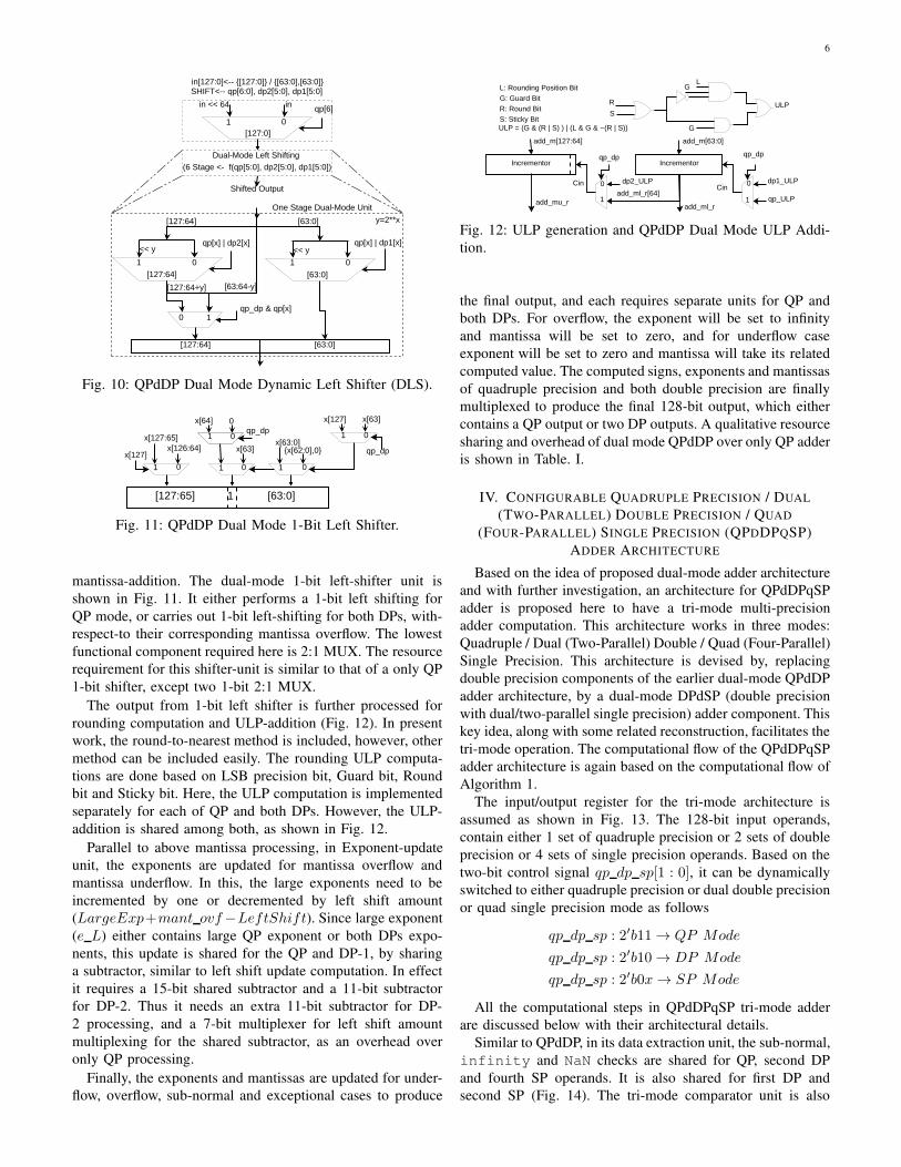
The output of dual-mode DLS then undergoes 1-bit left

shifting (normalization), in-case of mantissa overflow in

6

0101

0 1

y=2**x

<< y<< y

[63:0][127:64]

qp[x] | dp2[x] qp[x] | dp1[x]

[63:0][127:64]

qp_dp & qp[x]

[127:64+y] [63:64-y]

[63:0][127:64]

in

01

Shifted Output

SHIFT<-- qp[6:0], dp2[5:0], dp1[5:0]

in << 64 qp[6]

[127:0]

Dual-Mode Left Shifting (6 Stage <- f(qp[5:0], dp2[5:0], dp1[5:0])

in[127:0]<-- {[127:0]} / {[63:0],[63:0]}

One Stage Dual-Mode Unit

Fig. 10: QPdDP Dual Mode Dynamic Left Shifter (DLS).

[63:0][127:65] 1

x[127] {x[62:0],0}x[63:0]

1 000 11

qp_dp

x[127] x[63]

01qp_dp0

01

x[64]

x[63]x[127:65]

x[126:64]

Fig. 11: QPdDP Dual Mode 1-Bit Left Shifter.

mantissa-addition. The dual-mode 1-bit left-shifter unit is

shown in Fig. 11. It either performs a 1-bit left shifting for

QP mode, or carries out 1-bit left-shifting for both DPs, with-

respect-to their corresponding mantissa overflow. The lowest

functional component required here is 2:1 MUX. The resource

requirement for this shifter-unit is similar to that of a only QP

1-bit shifter, except two 1-bit 2:1 MUX.

The output from 1-bit left shifter is further processed for

rounding computation and ULP-addition (Fig. 12). In present

work, the round-to-nearest method is included, however, other

method can be included easily. The rounding ULP computa-

tions are done based on LSB precision bit, Guard bit, Round

bit and Sticky bit. Here, the ULP computation is implemented

separately for each of QP and both DPs. However, the ULP-

addition is shared among both, as shown in Fig. 12.

Parallel to above mantissa processing, in Exponent-update

unit, the exponents are updated for mantissa overflow and

mantissa underflow. In this, the large exponents need to be

incremented by one or decremented by left shift amount

(LargeExp+mant ovf−LeftShift). Since large exponent

(e L) either contains large QP exponent or both DPs expo-

nents, this update is shared for the QP and DP-1, by sharing

a subtractor, similar to left shift update computation. In effect

it requires a 15-bit shared subtractor and a 11-bit subtractor

for DP-2. Thus it needs an extra 11-bit subtractor for DP-

2 processing, and a 7-bit multiplexer for left shift amount

multiplexing for the shared subtractor, as an overhead over

only QP processing.

Finally, the exponents and mantissas are updated for under-

flow, overflow, sub-normal and exceptional cases to produce

qp_dp

add_m[127:64]

Incrementor

add_ml_r

Incrementor

add_mu_r

add_m[63:0]

Cin dp2_ULP

add_ml_r[64]

dp1_ULP

qp_ULP

qp_dp

0

11

0 Cin

L: Rounding Position BitG: Guard BitR: Round BitS: Sticky BitULP = (G & (R | S) ) | (L & G & ~(R | S))

R

S

G

GL

ULP

Fig. 12: ULP generation and QPdDP Dual Mode ULP Addi-

tion.

the final output, and each requires separate units for QP and

both DPs. For overflow, the exponent will be set to infinity

and mantissa will be set to zero, and for underflow case

exponent will be set to zero and mantissa will take its related

computed value. The computed signs, exponents and mantissas

of quadruple precision and both double precision are finally

multiplexed to produce the final 128-bit output, which either

contains a QP output or two DP outputs. A qualitative resource

sharing and overhead of dual mode QPdDP over only QP adder

is shown in Table. I.

IV. CONFIGURABLE QUADRUPLE PRECISION / DUAL

(TWO-PARALLEL) DOUBLE PRECISION / QUAD

(FOUR-PARALLEL) SINGLE PRECISION (QPDDPQSP)

ADDER ARCHITECTURE

Based on the idea of proposed dual-mode adder architecture

and with further investigation, an architecture for QPdDPqSP

adder is proposed here to have a tri-mode multi-precision

adder computation. This architecture works in three modes:

Quadruple / Dual (Two-Parallel) Double / Quad (Four-Parallel)

Single Precision. This architecture is devised by, replacing

double precision components of the earlier dual-mode QPdDP

adder architecture, by a dual-mode DPdSP (double precision

with dual/two-parallel single precision) adder component. This

key idea, along with some related reconstruction, facilitates the

tri-mode operation. The computational flow of the QPdDPqSP

adder architecture is again based on the computational flow of

Algorithm 1.

The input/output register for the tri-mode architecture is

assumed as shown in Fig. 13. The 128-bit input operands,

contain either 1 set of quadruple precision or 2 sets of double

precision or 4 sets of single precision operands. Based on the

two-bit control signal qp dp sp[1 : 0], it can be dynamically

switched to either quadruple precision or dual double precision

or quad single precision mode as follows

qp dp sp : 2′b11 → QP Mode

qp dp sp : 2′b10 → DP Mode

qp dp sp : 2′b0x → SP Mode

All the computational steps in QPdDPqSP tri-mode adder

are discussed below with their architectural details.

Similar to QPdDP, in its data extraction unit, the sub-normal,

infinity and NaN checks are shared for QP, second DP

and fourth SP operands. It is also shared for first DP and

second SP (Fig. 14). The tri-mode comparator unit is also

7

128-bit

64-bit15-bit

11-bit 52-bit

112-bit

11-bit 52-bit

23-bit 23-bit23-bit23-bit8-bit 8-bit 8-bit 8-bit

QP[127:96]/DP2[63:32]/SP4 QP[95:64]/DP2[31:0]/SP3 QP[63:32]/DP1[63:32]/SP2 QP[31:0]/DP1[31:0]/SP1

Fig. 13: QPdDPqSP Adder: Input/Output Register Format.

Data Extraction & SubNormal Handler

sp2_s1=in1[63], sp2_s2=in2[63]sp2_e1={in1[62:56],in1[55] | sp2_sn1}sp2_e2={in2[62:56],in2[55] | sp2_sn2}sp2_m1={~sp2_sn1,in1[54:32]}sp2_m2={~sp2_sn2,in2[54:32]}

sp1_s1 = in1[31], sp1_s2 = in2[31]sp1_e1={in1[30:24],in1[23]|sp1_sn1}sp1_e2={in2[30:24],in2[23]|sp1_sn2}sp1_m1={~sp1_sn1,in1[22:0]}sp1_m2={~sp1_sn2,in2[22:0]}

sp3_s1 = in1[95], sp3_s2 = in2[95]sp3_e1={in1[94:88],in1[87]|sp3_sn1}sp3_e2={in2[94:88],in2[87]|sp3_sn2}sp3_m1={~sp3_sn1,in1[86:64]}sp3_m2={~sp3_sn2,in2[86:64]}

sp4_s1 = in1[127], sp4_s2 = in2[127]sp4_e1={in1[126:120],in1[119] | sp4_sn1}sp4_e2={in2[126:120],in2[119] | sp4_sn2}sp4_m1={~sp4_sn1,in1[118:96]}sp4_m2={~sp4_sn2,in2[118:96]}

dp1_s1=in1[63], dp1_s2=in2[63]dp1_e1={in1[62:53],in1[52]|dp1_sn1}dp1_e2={in2[62:53],in2[52]|dp1_sn2}

dp1_m1={~dp1_sn1,in1[51:0]}dp1_m2={~dp1_sn2,in2[51:0]}

qp_s1=in[127], qp_s2=in2[127]qp_e1={in1[126:113],in1[112] | qp_sn1}qp_e2={in2[126:113],in2[112] | qp_sn2}qp_m1={~qp_sn1,in1[111:0]}qp_m2={~qp_sn2,in2[111:0]}

dp2_s1=in1[127], dp2_s2=in2[127]dp2_e1={in1[126:115],in1[116]|dp2_sn1}dp2_e2={in2[126:115],in2[116]|dp2_sn2}

dp2_m1={~dp2_sn1,in1[115:64]}dp2_m2={~dp2_sn2,in2[115:64]}

Comparator

sp2_in1-gt-in2 = (in1[62:32] > in2[62:32]) ? 1 : 0

sp1_in1-gt-in2 = (in1[30:0] > in2[30:0]) ? 1 : 0

sp3_in1-gt-in2 = (in1[94:64] > in2[94:64]) ? 1 : 0

sp4_in1-gt-in2 = (in1[126:96] > in2[126:96]) ? 1 : 0 sp4_in1-eq-in2 = (in1[126:96] == in2[126:96]) ? 1 : 0

sp2_in1-eq-in2 = (in1[62:32] == in2[62:32]) ? 1 : 0 sp3_in1-eq-in2 = (in1[94:64] == in2[94:64]) ? 1 : 0

SPs-Comparisons:

qp_in1-gt-in2 = dp2_in1-gt-in2 | ( dp2_in1-eq-in2 & ( (in1[63] & ~in2[63) | (in1[63] ~^ in2[63]) & dp1_in1-gt-in2) ) dp2_in1-eq-in2 = sp4_in1-eq-in2 & (in1[95] ~^ in2[95]) & sp3_in1-eq-in2 ? 1 : 0

QP-Comparison:

dp2_in1-gt-in2 = sp4_in1-gt-in2 | (sp4_in1-eq-in2 & ( (in1[95] & ~in2[95) | (in1[95] ~^ in2[95]) & sp3_in1-gt-in2) )

dp1_in1-gt-in2 = sp2_in1-gt-in2 | ( sp2_in1-eq-in2 & ( (in1[31] & ~in2[31) | (in1[31] ~^ in2[31]) & sp1_in1-gt-in2) ) DPs-Comparisons:

QP:

SP4:SP3:

SP1: SP2:DP1:

DP2:

in1[30:23] in2[30:23]

sp1_sn2sp1_sn1

sp1_sn

in1[62:55] in2[62:55]

sp2_sn2sp2_sn1

sp2_sn

in1[98:87] in2[98:87]

sp3_sn2sp3_sn1

sp3_sn

in1[126:119]in2[126:119]

sp4_sn2sp4_sn1

sp4_sn

dp2_sn2dp2_sn1

in1[115:112] in2[115:112]

qp_sn1 qp_sn2

qp_sn

sp2_sn2sp2_sn1

in1[54:52] in2[54:52]

dp1_sn1 dp1_sn2

dp1_sn

sp4_sn2sp4_sn1

in1[118:116] in2[118:116]

dp2_sn1 dp2_sn2

dp2_sn

Fig. 14: QPdDPqSP Adder: Data Extraction & Subnormal

Handler; Comparator.

shown in Fig. 14, which first compares all the SPs’ operands,

and then combines them to produce for both DPs’ operands

comparison. The DPs’ comparator outcomes are combined to

produce QP comparison result. This unit effectively requires

similar resources as in only QP comparator.

The SWAP unit of QPdDPqSP adder architecture is shown

in Fig. 15. Based on the mode of the operation, it initially

generates effective unified “greater than” signals (c1, c2, c3,and c4). The exponents of QP, both DPs and all SPs’ are then

multiplexed in to unified 32-bit exponents e1 (first exponent)

and e2 (second exponent). Each 8-bit of these e1 and e2 acts

as SPs’ exponents, or each 16-bit acts as DPs’ exponents, or

it will act for QP as a whole. Similarly, the mantissas are

multiplexed in to unified 128-bit m1 and m2. These unified

exponents and unified mantissas helps to have a tuned data-

path flow in the architecture, and enables to minimize the

multiplexing circuitry. Based on the effective “greater than”

signals (c1, c2, c3, and c4), unified exponents (e1 and e2) and

unified mantissas (m1 and m2), the small and large exponents,

and small and large mantissas are derived, which serves the

Unified Compare

0,1

3

2

qp_in1-gt-in2

C1dp1_in1-gt-in2

sp1_in1-gt-in2

qp_dp_sp

0,1

3

2

qp_in1-gt-in2

C2dp1_in1-gt-in2

sp2_in1-gt-in2

qp_dp_sp

0,1

3

2

qp_in1-gt-in2

C3dp2_in1-gt-in2

sp3_in1-gt-in2

qp_dp_sp

0,1

3

2

qp_in1-gt-in2

C4dp2_in1-gt-in2

sp4_in1-gt-in2

qp_dp_sp

OPsp1_op = sp1_s1 ~^ sp1_s2sp2_op = sp2_s1 ~^ sp2_s2sp3_op = sp3_s1 ~^ sp3_s2sp4_op = sp4_s1 ~^ sp4_s2dp1_op = dp1_s1 ~^ dp1_s2dp2_op = dp2_s1 ~^ dp2_s2qp_op = qp_s1 ~^ qp_s2

Large Signsp1_Ls = sp1_in1-gt-in2 ? sp1_s1 : sp1_s2sp2_Ls = sp2_in1-gt-in2 ? sp2_s1 : sp2_s2sp3_Ls = sp3_in1-gt-in2 ? sp3_s1 : sp3_s2sp4_Ls = sp4_in1-gt-in2 ? sp4_s1 : sp4_s2dp1_Ls = dp1_in1-gt-in2 ? dp1_s1 : dp1_s2dp2_Ls = dp2_in1-gt-in2 ? dp2_s1 : dp2_s2qp_Ls = qp_in1-gt-in2 ? qp_s1 : qp_s2

Unified Large Mantissa: Unified Small Mantissa:m_L[31:0]= c1 ? m1[31:0] : m2[31:0]m_L[63:32]= c2 ? m1[63:32] : m2[63:32]m_L[95:64]= c3 ? m1[95:64] : m2[95:64]m_L[127:96]= c4 ? m1[127:96] : m2[127:96]

m_S[31:0]= c1 ? m2[31:0] : m1[31:0]m_S[63:32]= c2 ? m2[63:32] : m1[63:32]m_S[95:64]= c3 ? m2[95:64] : m1[95:64]m_S[127:96]= c4 ? m2[127:96] : m1[127:96]

sp1_r_shift = SP ? shift[7:0] : 0

sp2_r_shift = SP ? shift[15:8] :0

sp3_r_shift = SP ? shift[23:16] :0

sp4_r_shift = SP ? shift[31:24] :0

dp1_r_shift = DP ? shift[10:0] : 0

dp2_r_shift = DP ? shift[26:16] :0

qp_r_shift = QP ? shift[14:0] : 0

Unified Exponentqp_dp_sp

e1{5’b0,dp2_e1,5’b0,dp1_e1}

{17’b0,qp_e1}

0,1

3

2

{sp4_e1,sp3_e1,sp2_e1,sp1_e1}

qp_dp_sp

e2{5’b0,dp2_e2,5’b0,dp1_e2}

{17’b0,qp_e2}

0,1

3

2

{sp4_e2,sp3_e2,sp2_e2,sp1_e2}

Unified Mantissa qp_dp_sp

m1{dp2_m1,11’b0,dp1_m1,11’b0}

{qp_m1,15’b0}

0,1

3

2

{sp4_m1,8’b0,sp3_m1,8’b0,sp2_m1,8’b0,sp1_m1,8’b0}

qp_dp_sp

m2{dp2_m2,11’b0,dp1_m2,11’b0}

{qp_m2,15’b0}

0,1

3

2

{sp4_m2,8’b0,sp3_m2,8’b0,sp2_m2,8’b0,sp1_m2,8’b0}

Unified Large Exponent:

Unified Small Exponent: e_S[7:0]= c1 ? e2[7:0] : e1[7:0] e_S[15:8]= c2 ? e2[15:8] : e1[15:8]e_S[23:16]= c3 ? e2[23:16] : e1[23:16] e_S[31:24]= c4 ? e2[31:24] : e1[31:24]

0

1

C1

e_L[7:0]e1[7:0]

e2[7:0]

0

1

C2

e_L[15:8]e1[15:8]

e2[15:8]

C3

0

1

e_L[23:16]e1[23:16]

e2[23:16]

0

1

e_L[31:24]e1[31:24]

e2[31:24]

C4

R_Shift_Amount

shift = e_L - e_S

Fig. 15: QPdDPqSP Adder: Swap: Large Sign, Exponent,

Mantissa and Operation; Right Shift Amount.

1 0

qp_shift[6:0]

1 0

out_hout_hv

{1’b1,out_l}{1’b0,out_h}

out_l out_lvLOD_32:5 LOD_32:5

1 0

out_hout_hv

{1’b1,out_l}{1’b0,out_h}

out_lout_lv

LOD_in[63:32] LOD_in[31:0]

LOD_32:5 LOD_32:5

sp2_shift[4:0] sp1_shift[4:0]

dp2_shift[5:0]

{1’b0,dp2_shift} {1’b1,dp1_shift}

dp1_shift[5:0]

sp3_shift[4:0]sp4_shift[4:0]

LOD_in[95:64]LOD_in[127:96]

LOD_64:6 LOD_64:6

Fig. 17: QPdDPqSP Tri-Mode Leading-One-Detector.

purpose for either of QP or DPs’ or SPs’. Furthermore, the

large sign and effective operation are computed for each modes

operands.

The next unit, also shown in Fig. 15, computes the right shift

amount for smaller mantissas. The shift amount is computed

by a 32-bit subtraction of unified large exponent e L and

unified small exponent e S. This serves the purpose for the

right shift amount of either of QP, or both DPs or all SPs, as

shown in Fig. 15.

The small mantissa is then right shifted by the tri-mode

dynamic right shifter unit (Fig. 16). The first stage of this

8

0101

01

[31:0]

0101

[63:32]

[31:0]

01

[31:0][63:32]

[63:32]

y=2**x

[127:0]

[63:0][127:64]

S4 S3 S2 S1

01

[63:0]

QP & qp[x]

[127:64]

[95:64][127:96]

One Stage (tri-mode) Unit (Stage-3 to Stage-7)

[95:64]

[95:64][127:96]

[127:96]

>> y >> y >> y >> y

D2 = (QP | DP) & (qp[x] | dp2[x])D1 = (QP | DP) & (qp[x] | dp1[x])

D1

[63-y:0][63+y:64]

[31+y:32] [31-y:0]

D2

S4 = qp[x] | dp2[x] | sp4[x]S3 = qp[x] | dp2[x] | sp3[x]S2 = qp[x] | dp1[x] | sp2[x]S1 = qp[x] | dp1[x] | sp1[x]

[95+y:96] [95-y:64]

in

01

qp[6]

[127:0]

in >> 64

SHIFT<-- qp[6:0], dp2[5:0], dp1[5:0] , sp4[4:0], sp3[4:0], sp2[4:0], sp1[4:0]

in[127:0]<-- {[127:0]} / {[63:0],[63:0]} / {31:0],[31:0],[31:0],[31:0]}

0101

01

[127:64] [63:0]

[127:64] [63:0]

[63:0][127:64]

qp[5] | dp2[5]>> 32 >> 32 qp[5] | dp1[5]

[95:64] [31:0]QP & qp[x]

Shifted Output

Stage-3 = f(qp[4], dp2[4], dp1[4], sp4[4], sp3[4], sp2[4], sp1[4])

Stage-4 = f(qp[3], dp2[3], dp1[3], sp4[3], sp3[3], sp2[3], sp1[3])

Stage-5 = f(qp[2], dp2[2], dp1[2], sp4[2], sp3[2], sp2[2], sp1[2])

Stage-6 = f(qp[1], dp2[1], dp1[1], sp4[1], sp3[1], sp2[1], sp1[1])

Stage-7 = f(qp[0], dp2[0], dp1[0], sp4[0], sp3[0], sp2[0], sp1[0])

QPdDPqSP Dynamic Right Shifter

sp1_op

m_L[31:0] m_S_shifted[31:0]

add_m1[32]

dp1_opqp_op

qp_dp_sp

sp2_op

0

m_S_shifted[63:32]

dp1_opqp_opqp_dp_sp

m_L[63:32]

0

qp_opqp_dp_sp

add_m2[32]

m_S_shifted[95:64]m_L[95:64]

dp2_opsp3_op

0

CLA Add/Sub 32-bit qp_opqp_dp_sp

add_m3[32]

dp2_opsp4_op

m_S_shifted[127:96]

add_m3[32:0] add_m2[32:0] add_m1[32:0]add_m4[32:0]

m_L[127:96]

QPdDPqSP Mantissa Addition/Subtraction

add_m[127:0] = {|add_m4[32:1], ((QP|DP)&add_m4[0]) | (SP&add_m3[32]), add_m3[31:1], (QP&add_m3[0]) | (DP|SP) & add_m2[32]),add_m2[31:1], ((QP|DP)&add_m2[0]) | (SP&add_m1[32]),add_m1[31:1]}

LOD_in1[127:0] = {|add_m4[32:31],add_m4[30:0], (QP|DP ? add_m3[31] : |add_m3[32:31]),add_m3[30:0], (QP ? add_m2[31] : |add_m2[32:31]),add_m2[30:0], (QP|DP ? add_m1[31] : | add_m1[32:31]),add_m1[30:0]}

CLA Add/Sub 32-bit CLA Add/Sub 32-bit CLA Add/Sub 32-bit

Fig. 16: QPdDPqSP Tri-Mode Dynamic Right Shifter and Mantissa Add/Sub.

0101

0 1

<< y<< y

[31:0]

0101

[63:32]

[31:0]

0 1

[31:0][63:32]

[63:32]

y=2**x

[31:32-y][63:32+y]

<< y<< y

[127:0]

[63:0][127:64]

S4 S3 S2 S1

0 1

[127:64+y] [63:64-y]

[63:0]

QP & qp[x]

[127:64]

[95:64][127:96]

One Stage (tri-mode) Unit (Stage-3 to Stage-7)in

01

in << 64 qp[6]

[127:0]

in[127:0]<-- {[127:0]} / {[63:0],[63:0]} / {31:0],[31:0],[31:0],[31:0]}

SHIFT<-- qp[6:0], dp2[5:0], dp1[5:0] , sp4[4:0], sp3[4:0], sp2[4:0], sp1[4:0]

0101

0 1

[63:0][127:64]

[63:0][127:64]

[63:0][127:64]

<< 32 << 32qp[5] | dp2[5] qp[5] | dp1[5]

[127:96] [63:32]

QP & qp[5]

Shifted Output

Stage-3 = f(qp[4], dp2[4], dp1[4], sp4[4], sp3[4], sp2[4], sp1[4])

Stage-4 = f(qp[3], dp2[3], dp1[3], sp4[3], sp3[3], sp2[3], sp1[3])

Stage-5 = f(qp[2], dp2[2], dp1[2], sp4[2], sp3[2], sp2[2], sp1[2])

Stage-6 = f(qp[1], dp2[1], dp1[1], sp4[1], sp3[1], sp2[1], sp1[1])

Stage-7 = f(qp[0], dp2[0], dp1[0], sp4[0], sp3[0], sp2[0], sp1[0])

[95:96-y][127:96+y][95:64]

[95:64][127:96]

[127:96]

D2 D1

QPdDPqSP Dynamic Left Shifter

S4 = qp[x] | dp2[x] | sp4[x]S3 = qp[x] | dp2[x] | sp3[x]S2 = qp[x] | dp1[x] | sp2[x]S1 = qp[x] | dp1[x] | sp1[x]

D2 = (QP | DP) & (qp[x] | dp2[x])D1 = (QP | DP) & (qp[x] | dp1[x])

[95:65][127:97] 1

x[127]

01

x[127:97]x[126:96]

1 1

x[94:64]x[95:65]

1 001

qp|dpx[127] x[95]0x[96]

x[95]

0101

x[62:32]x[63:33]

1 001

qpx[127] x[63]0x[64]

x[63]

0101qp

{x[30:0],0}x[31:0]

1 001

0x[32]

x[31]

01qp|dp

[63:33] [31:0]

x[127]qpx[63] dpspx[31]QPdDPqSP 1-bit Left Shifter

Cin

add_m[31:0]

sp1_ULPdp1_ULPqp_ULP

qp_dp_sp

Cin

add_m[63:32]

sp2_ULP

qp_dp_sp

add_m1_r

add_m1_r[32]

add_m2_radd_m2_r[32]

Cin

qp_dp_sp

add_m3_r

dp2_ULPsp3_ULPCin

Incrementor

qp_dp_sp

add_m4_radd_m3_r[32]

sp4_ULP

add_m[95:64]add_m[127:96]

QPdDPqSP Rounding ULP-Addition

Incrementor Incrementor Incrementor

Fig. 18: QPdDPqSP Tri-Mode Dynamic Left Shifter; 1-bit Left Shifter; and ULP Addition

9

TABLE I: Resource Sharing in QPdDPqSP Adder Sub-Components

Architectural

Components

QPdDP Adder Architecture QPdDPqSP Adder Architecture

Shared Resources Extra resource over Only QP Shared Resources Extra resource over Only QP

Data Extraction and Sub-

normal Handler

“Subnormal, infinity, and

NAN” checks of QP and

one DP

For one DP “Subnormal, infinity, and NAN”

check of QP, DP-2 and SP-4

For one DP, and two SPs

Comparator, Dynamic

Shifters, LOD

Shared QP and both DP Nil Shared QP, both DP and all SPs Nil

SWAP: Large Sign, Exp,

Mant and OP

Shared SWAP of QP and

both DP

Two 150-bit MUX, Control

Logic

Shared SWAP of QP, both DP and

all SPs

Two 160-bit 3:1 MUX, Control

Logic

Right Shift Amount Subtraction for QP and

both DP

7-bit sub, some bit-wise

ANDing

Subtraction for QP, both DP and all

SPs

17-bit sub, some bit-wise ANDing

Mantissa Add/Sub, Sum

Normalization

Shared QP and both DP two 1-bit 2:1 MUX and small

control logic

Shared QP, both DP and all SPs four 1-bit 3:1 MUX and small con-

trol logic

Left Shift Update Exponent difference of

QP and one DP

Remaining computation of

both DP

Exponent difference of QP, one DP,

and one SP

Remaining computation of both DP

and two SPs

1-bit Left Shifter Shared QP and both DP two 1-bit 2:1 MUX Shared QP, both DP and all SPs Six 1-bit 2:1 MUX and one 1-bit

3:1 MUX

Rounding ULP addition shared

among QP and both DP

ULP-computation of both DP ULP addition shared among QP,

both DP and all SPs

ULP-computation of both DP and

all SPs

Exponent Update Shared the update of QP

and one DP

Exponent Subtractor for one

DP and a 7-bit MUX

Shared the update of QP, one DP

and one SP

Exponent Subtractor for one DP

and two SP, and three 7-bit MUX

Final Processing Post Round Update of

Exponent and Mantissa

Remaining processing of both

DP, one 128-bit MUX to dis-

charge final output

Post Round Update of Exponent

and Mantissa

Remaining processing of both DP

and all SPs, one 128-bit 3:1 MUX

to discharge final output

shifter unit right shifts the input by 64-bit, and works for

QP purpose. The second stage works in dual mode fashion,

as in case on QPdDP, either for both DP or collectively

for QP. The remaining stages (stage 3-7) of this unit are

formed by combining the two dual mode stage of DPdSP

shifter, which collectively works in tri-mode, either for QP

or both DPs or four SPs, based on the effective mode of

the operation. Fig. 16 further shows the tri-mode mantissa

addition/subtraction module. It uses four 32-bit add/sub units

with control logic to accomplish this task. By combining their

outputs, this unit later generates the unified effective mantissa

addition/subtraction result add m and input LOD in for the

leading-one-detector, which contains the data either for QP, or

both DPs or all four SPs.

The LOD in is then fed in to the unified QPdDPqSP

tri-mode leading-one-detector, as shown in Fig. 17. The tri-

mode LOD contains two 64:6 LOD, each of which contains

two 32:5 LOD. The output of each 32:5 LOD gives the left

shift amount for each SPs’, which combines to produce left

shift amount for both DPs’ and QPs’. The same size LOD is

effectively required to accomplish the requirement of LOD for

only QP computation. The left shift amount is then updated

for sub-normal input cases, underflow cases (if left shift

amount exceeds or equal to the corresponding large exponent).

The underflow case requires the left shift amount equate to

exponent decrement by one. Since, the large exponents for all

mode is shared, the exponent decrement is shared among the

operands. One 7-bit decrement is shared for QP, first DP and

first SP, and one 6-bit decrement is shared for second DP and

third SP. Remaining SPs’ decrements are done separately.

Now, to shift the mantissa addition/subtraction result add m

by left shift amount, the QPdDPqSP tri-mode dynamic left

shifter is used (as shown in Fig. 18). The working principle

of tri-mode dynamic left shifter is similar to that of tri-mode

dynamic right shifter. Its first stage works for only QP, second

stage works in dual mode (either for QP or both DPs), and

remaining stages perform in tri-mode (either for QPs’ or both

DPs or all four SPs).

After left shifting of mantissa result, rounding is performed.

As in case of QPdDP, the ULP computation requires separate

units for each of QP, DPs’ and SPs’ as shown in Fig. 12.

The ULP addition is shared among all mode of the operation,

as shown in Fig. 18. Then each exponent is updated for

corresponding mantissa’s overflow or underflow, which needs

them to be either incremented by one or decremented by left

shift amount. This portion is shared as discussed for left shift

update. In the end, final normalization, and, exponents and

mantissas updates for exceptional cases are performed, and

output are multiplexed for a 128-bit output for given mode

of the operation. The resource overhead of QPdDPqSP adder

over only QP adder is shown in the Table-I.

The detailed implementation results of the dual mode

QPdDP and tri-mode QPdDPqSP adder architectures are

shown in the section V. It also discusses the comparisons with

the previous work available in the literature, along with the

improvements in the proposed architectures.

V. IMPLEMENTATION RESULTS AND COMPARISONS

Both of the proposed dual-mode QPdDP and tri-mode

QPdDPqSP architectures are implemented and synthesized for

standard-cell based ASIC platform. Synthesis is performed

using the UMC90 nm technology, using Synopsys Design

Compiler. An architecture for QP only adder is also designed

(using similar data path computational flow) and synthesized

for area & delay overhead measurements. These architectures

are designed with four pipeline stages (as shown in Fig. 1).

Similar architectures for DP only and SP only adders also syn-

thesized, using same computational flow. The implementation

details are shown in Table-II. Each module is synthesized with

the options of best possible clock-period, minimum-area, and

medium-effort for synthesis. Second pipeline stage in all the

architectures appears in critical path, and decides the clock-

period. The proposed architectures are functionally verified

for 5-millions random test cases in each mode, with different

pairs of operands, like normal-normal, subnormal-normal,

10

TABLE II: ASIC Implementation Details

SP DP QP QPdDP QPdDPqSP

Latency 4 4 4 4 4

Area(µm2) 16911 31863 76779 90116 91971

Area(gates) 5637 10621 25593 30038 30657

Period(ns) 0.78 0.95 1.1 1.16 1.45

Period(FO4) 17.33 21.11 24.44 25.78 32.22

Power(mw) 5.20 7.26 12.87 16.23 16.85

normal-subnormal and subnormal-subnormal; all mixed with

exceptional cases.

The proposed dual-mode QPdDP adder architecture requires

approximately 17% more hardware resources and roughly

5.45% extra period than only QP adder. Furthermore, the pro-

posed QPdDP adder requires approximately 35.86% smaller

area when compared with the combination of a QP only and

two-units of DP only adder ((QP+2*DP-QPdDP)/(QP+2*DP)).

Similarly, the tri-mode QPdDPqSP adder architectures re-

quires roughly 19.78% extra hardware and 31.81% large

period when compared to corresponding only QP adder.

However, when compared with the combination of a QP

only, two-units of DP only and four-units of SP only adder,

the QPdDPqSP adder requires roughly 55.81% smaller area

((QP+2*DP+4*SP-QPdDPqSP)/(QP+2*DP+4*SP)).

Literature contains very limited work on the dual-

mode QPdDP architecture, whereas the proposed tri-mode

QPdDPqSP adder architecture stands as a fresh proposal. A

comparison of dual-mode QPdDP architecture with previous

works is shown in Table-III. The related information for tri-

mode QPdDPqSP architecture are also included in Table-III,

to show its merit. The comparisons are carried out in terms

of % area and period/delay overhead over corresponding only

QP adder. This is to avoid different synthesis technologies of

earlier reported work. Moreover, the area is compared in terms

of gate-equivalent or scaled area equivalent, delay/period is

compared in terms of “Fan-Out-of-4’ (FO4) delay parameter,

and a unified comparison of area × period is performed,

all for a technology independent comparison. A. Akkas [15]

has proposed dual-mode architectures for QPdDP and DPdSP

adder with 250 nm technology. These architectures were pre-

sented for two sets of pipelining: 3-stage pipeline and 6-stage

pipeline. For their QPdDP architecture with 3-stage pipeline

they requires 15.3% more hardware and 14.12% more period

than their only QP design; and with 6-stage pipeline, the area-

overhead is 14% and period-overhead is 8.7%. Compared to

this architecture, the proposed QPdDP architecture has similar

area-overhead, but smaller delay-period overhead. Moreover,

the area × period of proposed architecture is much smaller

than QPdDP adder of [15]. Furthermore, the architectures

shown in [15] supports computation of only normalized

operands only, and it does not support sub-normal operands

computation and exceptional case handling.

Similarly, [16] has proposed dual-mode DPdSP and QPdDP

adder architectures, with two pipeline versions, 3-stage and

5-stage pipelines. These architectures do not provide compu-

tational support for sub-normal operands and without any ex-

ceptional case handling. These were synthesized with 110 nm

standard-cell ASIC library. For its 3-stage pipeline QPdDP de-

sign it has 35.8% area-overhead and 18.65% period overhead,

however, for its 5-stage design the area-overhead is 27.31%and period-overhead is 10.11%. Compared to this work, the

proposed dual-mode QPdDP architecture outperforms them

in terms of design overheads, as well as in terms of design

metrics: the area, period, and area× period.

Thus, compared to previous works, the proposed dual-

mode QPdDP adder architecture has smaller area-overhead and

delay-overhead when compared to only QP adder. The pro-

posed QPdDP architecture shows an improvement of approxi-

mately 50% in terms of unified metrics area×period product.

Furthermore, the proposed tri-mode QPdDPqSP architecture

also shows a promising design metrics, when compared to

dual-mode architectures, while being more computationally

strong. The proposed multi-mode architectures provides full

computational support to normal and sub-normal operands,

along with relevant exceptional case handling.

VI. CONCLUSIONS

This paper has presented two dynamically-configurable

multi-mode architectures for floating point adder, with on-the-

fly multi-precision support. The presented dual-mode QPdDP

and tri-mode QPdDPqSP architectures provides normal & sub-

normal computational support and exceptional case handling.

Both architectures are presented in fully pipelined format,

with 4-stages pipeline. The data path in both architectures

has been tuned with minimal required multiplexing circuitry.

The individual components of the architectures have been

constructed for on-the-fly multi-mode computation, with min-

imum required multiplexing. The dual-mode QPdDP adder ar-

chitecture needs approx 17% more resources and 5.45% more

delay-period than the QP only adder. Similarly, the tri-mode

QPdDPqSP adder architecture has approx 20% area overhead

and 32% delay overhead over QP only adder. In comparison to

previous works in literature, the proposed dual-mode QPdDP

design has approximately 50% smaller area×period product,

and has smaller area & delay overhead when compared to only

QP, and provide more computational support. Moreover, the

proposed tri-mode QPdDPqSP adder architecture stands as a

fresh proposal, while showing a promising design parameters

when compared with dual-mode QPdDP architectures. Our

future work is targeted towards the architectural exploration

of multi-mode fused multiplier adder (FMA) arithmetic unit.

REFERENCES

[1] “IEEE Standard for Floating-Point Arithmetic,” Tech. Rep., Aug. 2008.[2] H.-J. Oh, S. Mueller, C. Jacobi, K. Tran, S. Cottier, B. Michael,

H. Nishikawa, Y. Totsuka, T. Namatame, N. Yano, T. Machida, andS. H.Dhong, “A fully pipelined single-precision floating-point unit in thesynergistic processor element of a cell processor,” Solid-State Circuits,

IEEE Journal of, vol. 41, no. 4, pp. 759–771, 2006.[3] NXP Semiconductors, “AN10902 : Using the LPC32xx

VFP,” in Application note, Feb 2010. [Online]. Available:www.nxp.com/documents/application note/AN10902.pdf

[4] Nvidia, “NVIDIA’s Next Generation CUDATM ComputeArchitecture: KeplerTM GK110,” in White Paper, 2014.[Online]. Available: www.nvidia.com/content/PDF/kepler/NVIDIA-Kepler-GK110-Architecture-Whitepaper.pdf

[5] F. de Dinechin and G. Villard, “High precision numerical accuracy inphysics research,” Nuclear Instruments and Methods in Physics ResearchSection A: Accelerators, Spectrometers, Detectors and Associated Equip-

ment, vol. 559, no. 1, pp. 207–210, 2006.

11

TABLE III: Comparison of QPdDP Architecture with Related Work

QPdDP Architecture QPdDPqSP Architecture

[15] 250nm [16] 110nm Proposed 90nm Proposed 90nm

Latency 3 6 3 5 4 4

Area OH115.3% 14.01% 35.80% 27.31% 17.37% 19.78%

Period OH114.12% 8.71% 18.65% 10.11% 5.45% 31.81%

Scaled Area2 - - 239250 199723 90116 91971

Gate Count3 26967 33702 - - 30038 30657

Period (FO4)4 65.28 35.92 28.9 17.81 25.78 32.22

Scaled-Area2 × FO4-Period4 (106) - - 6.91 3.55 2.32 2.96

Gate-Count3 × FO4-Period4 (106) 1.76 1.21 - - 0.77 0.98

1Area/Period OH = (QPdDP - QP) / QP, 2in µm2 @ 90nm = (Area @ 110nm) * (90/110)23Based on minimum size inverter 41 FO4 (ns) ≈ (Tech. in µm) / 2

[6] D. H. Bailey, R. Barrio, and J. M. Borwein, “High-precision compu-tation: Mathematical physics and dynamics,” Applied Mathematics and

Computation, vol. 218, no. 20, pp. 10 106–10 121, 2012.[7] A. Baluni, F. Merchant, S. K. Nandy, and S. Balakrishnan, “A fully

pipelined modular multiple precision floating point multiplier withvector support,” in Electronic System Design (ISED), 2011 International

Symposium on, 2011, pp. 45–50.[8] K. Manolopoulos, D. Reisis, and V. Chouliaras, “An efficient multiple

precision floating-point multiplier,” in Electronics, Circuits and Systems

(ICECS), 2011 18th IEEE International Conference on, 2011, pp. 153–156.

[9] A. Akkas and M. J. Schulte, “A quadruple precision and dual doubleprecision floating-point multiplier,” in Proceedings of the Euromicro

Symposium on Digital Systems Design, ser. DSD ’03, 2003, pp. 76–.[10] ——, “Dual-mode floating-point multiplier architectures with parallel

operations,” Journal of System Architecture, vol. 52, no. 10, pp. 549–562, Oct. 2006.

[11] D. Tan, C. E. Lemonds, and M. J. Schulte, “Low-power multiple-precision iterative floating-point multiplier with simd support,” IEEE

Trans. Comput., vol. 58, no. 2, pp. 175–187, Feb. 2009.[12] L. Huang, L. Shen, K. Dai, and Z. Wang, “A new architecture for

multiple-precision floating-point multiply-add fused unit design,” inComputer Arithmetic, 2007. ARITH ’07. 18th IEEE Symposium on, 2007,pp. 69–76.

[13] M. Gok and M. M. Ozbilen, “Multi-functional floating-point maf designswith dot product support,” Microelectron. J., vol. 39, no. 1, pp. 30–43,Jan. 2008.

[14] A. Isseven and A. Akkas, “A dual-mode quadruple precision floating-point divider,” in Signals, Systems and Computers, 2006. ACSSC ’06.Fortieth Asilomar Conference on, 2006, pp. 1697–1701.

[15] A. Akkas, “Dual-Mode Quadruple Precision Floating-Point Adder,”Digital Systems Design, Euromicro Symposium on, vol. 0, pp. 211–220,2006.

[16] ——, “Dual-mode floating-point adder architectures,” Journal of Sys-

tems Architecture, vol. 54, no. 12, pp. 1129–1142, Dec. 2008.[17] M. Ozbilen and M. Gok, “A multi-precision floating-point adder,” in

Research in Microelectronics and Electronics, 2008. PRIME 2008.

Ph.D., 2008, pp. 117–120.[18] M. Jaiswal, R. Cheung, M. Balakrishnan, and K. Paul, “Unified ar-

chitecture for double/two-parallel single precision floating point adder,”Circuits and Systems II: Express Briefs, IEEE Transactions on, vol. 61,no. 7, pp. 521–525, July 2014.

[19] ——, “Configurable architecture for double/two-parallel single precisionfloating point division,” in VLSI (ISVLSI), 2014 IEEE Computer Society

Annual Symposium on, July 2014, pp. 332–337.

Manish Kumar Jaiswal (S’12–M’14) is currentlya Post-Doctorate Fellow in Dept. of EEE at TheUniversity of Hong Kong. He received his B.Sc.and M.Sc. in Electronics from D.D.U. GorakhpurUniversity in 2002 & 2004 respectively. He obtainedhis M.S.(By Research) from EE Dept. - I.I.T. Madrasin 2009 and Ph.D. from EE Dept. - City Universityof Hong Kong in 2014. He received OutstandingAcademic Performance award during his Ph.D. atCityU-HK. He worked as a Lecturer in the Dept.of Electronics at D.D.U. Gorakhpur University for

a year (2005-06), and as a Faculty Member in Dept. of EE at The ICFAIUniversity, Dehradun, India, for two years (2009-11). He also spent 6-months in IBM India Pvt. Ltd. Bangalore in 2008, as a project intern. Hisresearch interest includes Digital VLSI Design, Reconfigurable Computing,ASIC/FPGA SoC Design, VLSI Implementation of DSP, Biomedical VLSIand High-Performance Algorithmic Synthesis.

B. Sharat Chandra Varma is a Postdoctoral Re-search Fellow at the Department of Electronic andElectrical Engineering in The University of HongKong. He received his PhD from Amarnath andShasi Khosla School of Information Technology atthe Indian Institute of Technology Delhi, India inJanuary 2015. He holds a Masters degree in VLSI-CAD from Manipal University, India and did hisBachelors of Engineering degree in Electronics andCommunications Engineering from ViswesvarayaTechnological University, India. He has also worked

as a Software Engineer with QuickLogic India Pvt. Ltd. for one year, where hedeveloped CAD tools for QuickLogic FPGAs. His research interests includeFPGA, hardware accelerators, hardware-software co-design and VLSI.

Hayden K. H. So (S’03-M’07) received the B.S.,M.S., and Ph.D. degrees in electrical engineeringand computer sciences from University of California,Berkeley, CA in 1998, 2000, and 2007 respectively.He is currently an Assistant Professor of in theDepartment of Electrical and Electronic Engineeringat the University of Hong Kong. He received theCroucher Innovation Award in 2013 for his workin power-efficient high-performance heterogeneouscomputing system. He was also awarded the Univer-sity Outstanding Teaching Award (Team) in 2012, as

well as the Faculty Best Teacher Award in 2011.

12

M. Balakrishnan is a Professor in the Departmentof Computer Science & Engineering at I.I.T. Delhi.He obtained his B.E.(Hons.) in Electronics & Elec-trical Engg. from BITS Pilani in 1977 and Ph.D.from EE Dept. IIT Delhi in 1985. He worked as aScientist in CARE, IIT Delhi from 1977 to 1985where he was involved in designing and implement-ing real-time DSP systems. For the last 27 years, heis involved in teaching and research in the areas ofdigital systems design, electronic design automationand embedded systems. He has supervised 10 Ph.D.

students, 3 MSR students, 145 M.Tech/B.Tech projects and published nearly100 conference and journal papers. Further, he has held visiting positionsin universities in Canada, USA and Germany. At IIT Delhi, he has beenthe Philips Chair Professor, Head of the Department of Computer Science& Engineering, Dean of Post Graduate Studies & Research at IIT Delhiand Deputy Director (Faculty) at IIT Delhi. His research interests includeembedded systems design, low power and system level design. Currently he isinvolved in developing a number of assistive devices for the visually impaired.

Kolin Paul is an Associate Professor in the De-partment of Computer Science and Engineering atIIT Delhi India. He received his B.E. degree inElectronics an Telecommunication Engineering fromNIT Silchar in 1992 and Ph.D. in Computer Sciencein 2002 from BE College (DU), Shibpore. During2002-03 he did his post doctoral studies at Col-orado State University, Fort Collins, USA. He haspreviously worked at IBM Software Labs. His lastappointment was as a Lecturer in the Department ofComputer Science at the University of Bristol, UK.

His research interests are in understanding high performance architecturesand compilation systems. In particular he works in the area of Adap-tive/Reconfigurable Computing trying to understand its use and implicationsin embedded systems.

Ray C.C. Cheung (M’07) received the B.Eng.and M.Phil. degrees in computer engineering andcomputer science and engineering at the ChineseUniversity of Hong Kong (CUHK), Hong Kong, in1999 and 2001, respectively, and the Ph.D. degreein computing at Imperial College London, London,U.K., in 2007. In 2009, he worked as a visitingresearch fellow in the Department of Electrical En-gineering, Princeton University. He is currently anassistant professor at City University of Hong Kong(CityU). His research team, CityU Architecture Lab

for Arithmetic and Security (CALAS) focuses on the following researchtopics: reconfigurable trusted computing, SoC VLSI designs, cryptography,and embedded biomedical VLSI designs.