Confidence Intervals z Learn and Confirm Cycle …holford.fmhs.auckland.ac.nz/.../bootstrap-and-confidence-intervals.pdf · » Confidence intervals are often asymmetric The standard

Slide 1

Bootstrap and

Confidence Intervals

Nick Holford

Dept Pharmacology & Clinical Pharmacology

University of Auckland, New Zealand

Slide 2

©NHG Holford, 2015, all rights reserved.

Learn and Confirm Cycle

Original idea from GE Box (1966)

Translated to Drug Development

Sheiner LB. Learning versus confirming in

clinical drug development. Clinical

Pharmacology & Therapeutics

1997;61(3):275-91

Sheiner brought the idea of a learn and confirm cycle to drug development. The basic idea was originally devised by George Box (a famous statistician)

Slide 3


Confirming or Learning?

Confirming tests the Yes/No Hypothesis

If the question being asked has a

Yes/No answer then it is a Confirming

question

If the question has a How Much answer

then it is a Learning question

Confirming and learning require different kinds of answers.

Slide 4


Confirming

• Making sure

• Outcome Expected

• Analysis Assumptions MinimizedE.g. Randomized Treatment Assignment

• Questions for Drug Approval– E.g.

• Does the drug work?

• Can it be used safely in renal failure?

Learning

• Exploration

• Outcome Unexpected

• Assumption rich analysis

–E.g. PKPD model

• Questions for Drug Science

–E.g.

• How big an effect does the drug have?

• What is the clearance in renal failure?

Confirming or Learning?

Power Bias & Imprecision

Confirming answers are Yes or No. The rejection of the null hypothesis to accept a model answers the question ‘Is this model better than the other?’. It is therefore a confirming question. Simulation can be used to define the power of a clinical trial to reject the null hypothesis. Learning answers describe how big something is. Estimation of model parameters answers learning type questions. Simulation can be used to learn the bias and imprecision of parameter estimates.

Slide 5


Confidence in Population Models

How confident can you be in parameter

estimates?

Typical statistics

» standard error

» 95% confidence interval

Examining the distribution of uncertainty in parameter estimates is used to identify the standard error of the uncertainty (imprecision) and calculate a confidence interval.

Slide 6


The Standard Error Problem

Standard errors (SE) are not confidence intervals (CI)

CI using SE assumes a model – usually normal distribution

Normal distribution is symmetrical

What is the problem when using NONMEM?» Standard errors are asymptotic estimates

– And may be unobtainable even if the model fit is good

» Confidence intervals are often asymmetric

The standard error is of no use by itself. It can be used to compute a confidence interval under the assumption that the uncertainty is normally distributed. This is usually unreasonable for non-linear model parameters (such as Emax). It is common to find asymmetry in the uncertainty of a parameter.

Slide 7


Log Likelihood Profile

Assume that change in log likelihood with different parameter values is Chi-square distributed

Fix parameter of interest and refit the data

Find parameter values which change log likelihood by CHIINV(1-CI,df=1) e.g. 3.84 for 95% CI

The log likelihood profile method does not assume symmetry of the parameter uncertainty but it does use the likelihood ratio test (LRT) based on the change in NONMEM objective function value to predict the probability of the confidence interval. This assumption is known to be only approximately true (see discussion of the randomization test).

Slide 8


Log Likelihood Profile

Tacrine Potency Parameter

Holford NHG, Peace KE. Results and validation of a population pharmacodynamic model for cognitive effects in Alzheimer

patients treated with tacrine. Proceedings of the National Academy of Sciences of the United States of America

1992;89(23):11471-11475

+

+

+

+

+

+

+

+

-4.4 -3.6 -2.8 -2.0 -1.2 -0.4

10

8

4

D

e

l

t

a

O

B

J

βA

2

6

A log likelihood profile (LLP) is illustrated here. The parameter is BetaA the potency parameter for the effect of tacrine at a dose of 80 mg/day. The approximate 95% confidence interval is shown under the assumption of the chi-square distribution. This LLP was obtained using the FO method and therefore the actual 95% CI is almost certainly wider than shown here.

Slide 9


Resampling Methods

Jackknife (Quenouille 1949)

» Used to estimate bias

» Tukey (1958) proposed its use to estimate

variance

Bootstrap (Effron 1979)

“A data set of size n has 2n-1 nonempty

subsets; the jackknife uses only n of them.

The jackknife may be improved by using

statistics based on … all 2n-1subsets.”

Shao & Tu 1995

Resampling methods have been proposed as a means to take advantage of the assumption that observations in a data set differ randomly and it is this random difference that gives rise to the uncertainty in a parameter. The Jackknife method takes subsets of the original data and obtains estimates of the parameter of interest. These are then combined to obtain an overall parameter estimate to describe the mean or the variance. The bootstrap is similar to the jackknife but creates datasets the same size as the original by re-sampling at random from the original data. This means that the same observation can appear more than once in the data set. Under the assumption that the random component of the observation is indeed random from observation to observation then it does not matter that an observation is resampled. The bootstrap method means that many more random data sets can be generated and this opens up the possibility to estimate more interesting statistics such as confidence intervals.

Slide 10


Theoretical and Empirical

Distributions

Theoretical distribution is based on a

mathematical model for the distribution

that might have given rise to the data

e.g. normal

Empirical distribution is derived from

data

It is helpful to distinguish theoretical and empirical distributions. The bootstrap procedure constructs an empirical distribution. This is especially useful because the theoretical distribution may not be known.

Slide 11


Bootstrap Methods

Davison & Hinkley

1997

Simulation methods

» Parametric

» Non-Parametric

Davison & Hinkly describe the theory and application of bootstrap methods. They distinguish parametric bootstraps which rely on using parametric model to simulate data and non-parametric bootstraps which rely on resampling to obtain new randomly different datasets from original data.

Slide 12


Bootstrap Samples

Parametric Sampling

» Use a parametric model to simulate and

sample from the theoretical distribution

Non-parametric Sampling

» Use the data and sample from the

empirical distribution

Compute statistics (e.g. 95% CI) from

the Sample

Both the parametric and non-parametric bootstrap procedures can be used to generate samples from their respective distributions. The parametric method requires a full parametric model (e.g. PK model with population parameter variability and residual unidentified variability) while the non-parametric method only requires an original data set.

Slide 13


Non-Parametric Bootstrap#Data is the empirical dist vector Fhat[] of length NSUB#Let NBOOT be the number of bootstrap samples

for (i=1; i <= NBOOT; i++ ) {

#Sample the elements of Fhat NSUB times using a uniform random distribution

for ( j=1; j <= NSUB; j++ ){

jsub=int(NSUB*uran)+1

BS[j] = Fhat[jsub]

}

#Estimate parameter from the bootstrap sample e.g. the average

Thetastar[i] = average(BS)

}

#Describe the distribution of Thetastar e.g. standard error

se = stdev(Thetastar)

The basic bootstrap algorithm is shown using awk code. NBOOT is the number of bootstrap samples requested. This would typically be 1000 or more to obtain an estimate of the 95% confidence interval. Fhat is the empirical distribution i.e. the original data set. BS is a bootstrap data set obtained by resampling from Fhat. Nsub is the number of subjects. Thetastar is a vector of parameter estimates. In this case the average is computed for each BS sample data set. This step in the algorithm can be much more complex e.g. a NONEMM run using the BS data set can be used to estimate a full set of parameters. In the last line of the algorithm a meta-analysis procedure is used to examine the results in Thetastar. In this case the standard deviation of the average values in Thetastar is used to estimate the standard error. The same Thetastar array could also be used to find the 90% confidence interval by looking for the values of Thetastar that are less than the 5%centile and greater than the 95%centile.

Slide 14


Resampling for Regression

Model Based Resampling

» Fit model and then sample from residuals

– But problem with heteroscedastic error

Resampling Cases

» Sampling unit is a “case” of X,Y pairs

– But distorts original design

» Population analysis samples individuals as the “case”

*

10

*

jjj XY

ijij XXYY **

;

Davison & Hinckley point out the difficulty of sampling random observations when doing regression. Ideally one would sample from the residuals of the regression predictions but it there is heteroscedasticity then this cannot be done simply. The alternative is to sample from each subject as a ‘case’. This preserves the heteroscedasticity but distorts the design of the trial if there is substantial difference from subject to subject in their dose and sampling times. It seems unlikely that these design differences would be important in determining the outcome of typical PKPD data analyses.

Slide 15


WFN nmbs

Any model/data

» Care with paths for user defined $SUB

WFN command:

nmbs theopd 1 1000

Results in theopd.bs directory in theopd.txt

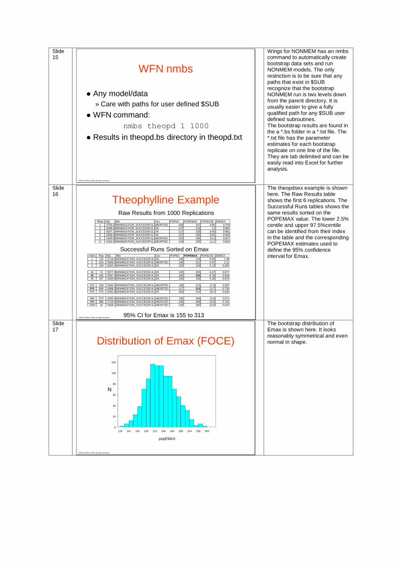
Wings for NONMEM has an nmbs command to automatically create bootstrap data sets and run NONMEM models. The only restriction is to be sure that any paths that exist in $SUB recognize that the bootstrap NONMEM run is two levels down from the parent directory. It is usually easier to give a fully qualified path for any $SUB user defined subroutines. The bootstrap results are found in the a *.bs folder in a *.txt file. The *.txt file has the parameter estimates for each bootstrap replicate on one line of the file. They are tab delimited and can be easily read into Excel for further analysis.

Slide 16


Theophylline ExampleRaw Results from 1000 Replications

Successful Runs Sorted on Emax

95% CI for Emax is 155 to 313

#Rep Obj Min Cov POPE0 POPEMAX POPEC50 EMSEX

1 5793.0 MINIMIZATION_SUCCESSFUL_R_MATRIX_ALGORITHMICALLY_NON-POSITIVE-SEMIDEFINITE_BUT_NONSINGULAR_COVARIANCE_STEP_ABORTED_ABORTED 158 147 8.85 0.754

2 5468.5 MINIMIZATION_SUCCESSFUL_OK 147 216 11 0.891

3 6037.1 MINIMIZATION_SUCCESSFUL_OK 127 230 9.05 0.801

4 5556.8 MINIMIZATION_SUCCESSFUL_OK 137 205 8.91 0.932



Index Rep Obj Min Cov POPE0 POPEMAX POPEC50 EMSEX

1 732 5719.6 MINIMIZATION_SUCCESSFUL_OK 148 116 6.64 1.38

2 216 5936.6 MINIMIZATION_SUCCESSFUL_R_MATRIX_ALGORITHMICALLY_NON-POSITIVE-SEMIDEFINITE_BUT_NONSINGULAR_COVARIANCE_STEP_ABORTED_ABORTED 148 121 4.97 1.11











The theopdsex example is shown here. The Raw Results table shows the first 6 replications. The Successful Runs tables shows the same results sorted on the POPEMAX value. The lower 2.5% centile and upper 97.5%centile can be identified from their index in the table and the corresponding POPEMAX estimates used to define the 95% confidence interval for Emax.

Slide 17


Distribution of Emax (FOCE)

116 141 165 190 215 240 264 289 314 338 363

popEMAX

0

20

40

60

80

100

120

N

The bootstrap distribution of Emax is shown here. It looks reasonably symmetrical and even normal in shape.

Slide 18


Distribution of EMSex (FOCE)

0.52 0.60 0.69 0.77 0.86 0.95 1.03 1.12 1.21 1.29 1.38

EMSex

0

50

100

150

200

N

3.2%

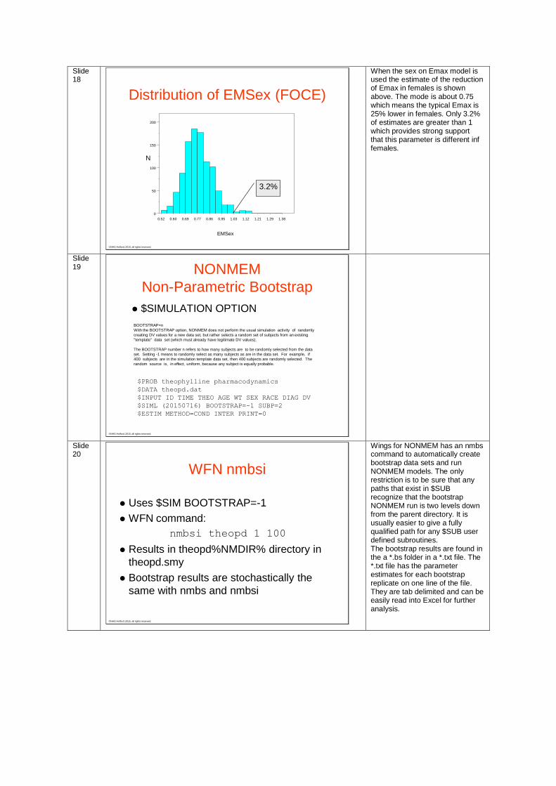
When the sex on Emax model is used the estimate of the reduction of Emax in females is shown above. The mode is about 0.75 which means the typical Emax is 25% lower in females. Only 3.2% of estimates are greater than 1 which provides strong support that this parameter is different inf females.

Slide 19


NONMEM

Non-Parametric Bootstrap

$SIMULATION OPTION

BOOTSTRAP=n

With the BOOTSTRAP option, NONMEM does not perform the usual simulation activity of randomly

creating DV values for a new data set, but rather selects a random set of subjects from an existing

"template" data set (which must already have legitimate DV values).

The BOOTSTRAP number n refers to how many subjects are to be randomly selected from the data

set. Setting -1 means to randomly select as many subjects as are in the data set. For example, if

400 subjects are in the simulation template data set, then 400 subjects are randomly selected. The

random source is, in effect, uniform, because any subject is equally probable.

$PROB theophylline pharmacodynamics

$DATA theopd.dat

$INPUT ID TIME THEO AGE WT SEX RACE DIAG DV

$SIML (20150716) BOOTSTRAP=-1 SUBP=2

$ESTIM METHOD=COND INTER PRINT=0

Slide 20


WFN nmbsi

Uses $SIM BOOTSTRAP=-1

WFN command:

nmbsi theopd 1 100

Results in theopd%NMDIR% directory in

theopd.smy

Bootstrap results are stochastically the

same with nmbs and nmbsi

Wings for NONMEM has an nmbs command to automatically create bootstrap data sets and run NONMEM models. The only restriction is to be sure that any paths that exist in $SUB recognize that the bootstrap NONMEM run is two levels down from the parent directory. It is usually easier to give a fully qualified path for any $SUB user defined subroutines. The bootstrap results are found in the a *.bs folder in a *.txt file. The *.txt file has the parameter estimates for each bootstrap replicate on one line of the file. They are tab delimited and can be easily read into Excel for further analysis.

Slide 21


Parametric Bootstrap Random effects (parameters and residual error) are

simulated instead of sampling from original dataset

Fixed effects may use the same covariate distribution

as original dataset or use simulated covariate

distribution

Distribution of bootstrap parameter estimates can be

used to calculate estimation bias

“Gold Standard” method for imprecision (confidence

intervals, standard error)

Slide 22


What is the Truth?

Bias: Easy

» True parameters for fixed and random effects used for simulation

» Compared to bootstrap average estimate

Uncertainty: Tricky

» 95SE: Standard error describing the 95% bootstrap confidence

interval for the parameters

» Compared to bootstrap average asymptotic standard error

Slide 23


NONMEM and Monolix

Estimation Methods Parametric Bootstrap

» 100 simulated data sets

» Initial estimates “jitter” x 3 or x 1/3 true value (J3)

NONMEM

» FOCEI

» AUTO (SAEM ln mu-transformed)

» A10k1k (like AUTO but 10,000 burnin, 1,000 accumulation)

Monolix

» SAEM (ln transformed internally)

» p5p2 (500 burnin, 200 accumulation, Auto option)

» A10k1k (like p5p2 but 10,000 burnin, 1,000 accumulation)

Slide 24


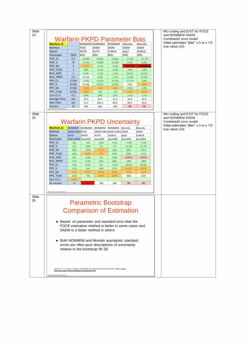
Warfarin PKPD Parameter BiasWarfarin J3 NONMEM NONMEM NONMEM Monolix MonolixMethod FOCE SAEM SAEM SAEM SAEMOption INTER AUTO A10k1k p5p2 A10k1kParameter TRUE MDL MDL MDL MDL MDLPOP_CL 0.1 -0.09% 0.58% 0.56% -11.8% -11.7%

POP_V 8 17.2% -0.08% -0.10% 9.2% 9.2%

POP_KA 2 222% -4.5% -5.0% 370084% #########

POP_TLAG 1 48% -3.5% -4.5% -19% -18%

RUV_ADD 1 5.6% -1.3% -1.4% 19.1% 19.1%

RUV_PROP 0.1 57.2% 2.0% 2.2% 11.6% 12.0%

PPV_CL 0.316 -4.3% -0.51% -0.51% -17.7% -18%

PPV_V 0.316 57.4% 0.45% 0.40% 57% 80%

PPV_KA 0.316 130% -63% -66% 4.9% 4.9%

PPV_TLAG 0.316 338% -9% -7% 102% 103%

Corr CL V 0.1 0.8% 24% 23% -239% -238%

Average Time sec 10.3 53.5 51.3 42.0 42.4

Max Time sec 51.5 102.5 80.6 82.0 91.0

Success % 100 100 100 98 98

MU coding and EXIT for FOCE and NONMEM SAEM Combined2 error model Initial estimates “jitter” x 3 or x 1/3 true value (J3)

Slide 25


Warfarin PKPD UncertaintyWarfarin J3 NONMEM NONMEM NONMEM NONMEM Monolix Monolix

Method SAEM lnMU FOCE SAEM lnMU SAEM lnMU SAEM SAEM

Option AUTO INTER AUTO A10k1k p5p2 A10k1k

Parameter 95SE SAEM AsymRSE AsymRSE AsymRSE AsymRSE AsymRSE

POP_CL 6% -5% 10% 11% -7.4% -7.2%

POP_V 6% -19% 7% 7% 11.5% 12.7%

POP_KA 29% -47% 171% 36% 46% 45%

POP_TLAG 18% -80% 75% 47% 29% 31%

RUV_ADD 6% -23% 7% 4.0% 3185% 3190%

RUV_PROP 11% 1.4% 43% 36% -28% -28%

PPV_CL 15% -8.5% 5% -2.3% 29.6% 39.8%

PPV_V 12% -6% 28% 27% 643% 647%

PPV_KA 77% 101% 364% 359% -83% -83%

PPV_TLAG 42% -7% 163% 145% 50% 52%

Corr CL V 158%

SE success % 5 100 100 98 98

MU coding and EXIT for FOCE and NONMEM SAEM Combined2 error model Initial estimates “jitter” x 3 or x 1/3 true value (J3)

Slide 26


Parametric Bootstrap

Comparison of Estimation

Based on parameter and standard error bias the

FOCE estimation method is better in some cases and

SAEM is a better method in others

Both NONMEM and Monolix asymptotic standard

errors are often poor descriptions of uncertainty

relative to the bootstrap 95 SE

Holford, N. H. G. (2014). Evaluation of NONMEM and Monolix by Parametric Bootstrap. PAGE. Alicante.

http://www.page-meeting.org/default.asp?abstract=3143

Slide 27


Practical Matters

What if my preferred final model does

not complete the $COV step?

What do I do with bootstrap runs that do

not minimize successfully?

With simple data sets it is common for nearly all boostrap runs to complete successfully. It is not usual to run the $COV step at the same time because this takes extra time and the $COV estimates are not as useful as the bootstrap estimates of uncertainty. However, with more complex problems NONMEM may finish in a variety of ways these include: 1) $COV OK 2) Minimization successful but $COV failed 3) Minimization terminated due to rounding errors 4) Other errors eg. Next iteration would produce an infinite objective function value.

Slide 28


Methods

Original Data set (Matthews et al. 2004)

» 697 patients; 2567 concentrations

Final Model terminated» MINIMIZATION TERMINATED DUE TO PROXIMITY OF LAST ITERATION

EST. TO A VALUE AT WHICH THE OBJ. FUNC. IS INFINITE

Matthews I, Kirkpatrick C, Holford NHG. Quantitative justification for target concentration intervention - Parameter

variability and predictive performance using population pharmacokinetic models for aminoglycosides. British Journal of

Clinical Pharmacology 2004;58(1):8-19

A recent publication has used bootstraps to obtain confidence intervals on parameters for a model that terminated with ‘MINIMIZATION TERMINATED DUE TO PROXIMITY OF LAST ITERATION EST. TO A VALUE AT WHICH THE OBJ. FUNC. IS INFINITE’. This model was preferred as the final model because it expressed a pathophysiological reason for why some patients have low serum creatinine concentrations in comparison to their expected aminoglycoside clearance.

Slide 29


The Final Model Context

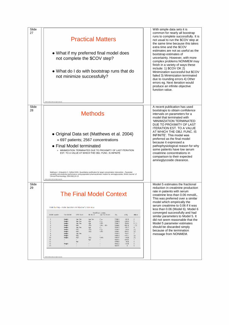
Model 5 estimates the fractional reduction in creatinine production rate in patients with serum creatinine less than 0.06 mmol/L. This was preferred over a similar model which empirically the serum creatinine to 0.06 if it was less than 0.06 (Model 6). Model 6 converged successfully and had similar parameters to Model 5. It did not seem reasonable that the Model 5 parameter estimates should be discarded simply because of the termination message from NONMEM.

Slide 30


Methods II

Original Data Set

» Bootstrap of final model

» Initial estimates equal to final estimates at

termination

Simulated Data Set

» Model identical to Original Data

» Parameters obtained from average of 1055

bootstrap runs of original data

» Bootstrap of a single simulated data set

Bootstraps were performed on the original data and also a data set obtained by simulating from the mean boostrap parameters obtained from the original data set.

Slide 31


Methods III

Compilers

» Compaq Visual Fortran 6.6 Update C

– F77OPT =/fltconsistency /optimize:4 /fast

» GNU Fortran (GCC 3.1) 3.1 20020514

– F77OPT =-fno-backslash –O

Platform

» Windows 2000

» Dual AMD MP2000

Two compilers were compared. The Compaq df compiler is aggressively optimized while the GNU g77 compiler uses default optimization. It was expected that the GNU compiler might have better numerical performance while the df compiler would be faster. All runs were performed on AMD MP2000 processors.

Slide 32


NONMEM Termination Type

Data df Data g77 Sim df

Runs 3141 924 3125

SUCCESS 30% 27% 46%

$COV 18% 9% 15%

INF OBJ 9% 12% 10%

The two compilers gave broadly similar results for the types of termination. However, somewhat unexpectedly the g77 compiler was only able to complete the covariance step in half of the runs for which the df compiler was successful. The simulated data set had more successful runs but % lower successful $COV.

Slide 33


THETA

0.0

0.2

0.4

0.6

0.8

1.0

3.0 3.5 4.0

CLR

Estimate

Pro

po

rtio

n<

=E

stim

ate

Aminoglycoside Data PK

CovSxsInf

0.0

0.2

0.4

0.6

0.8

1.0

3.2 3.4 3.6 3.8 4.0 4.2

CLR

Estimate

Pro

po

rtio

n<

=E

stim

ate

Aminoglycoside Simulated PK

CovSxsInf

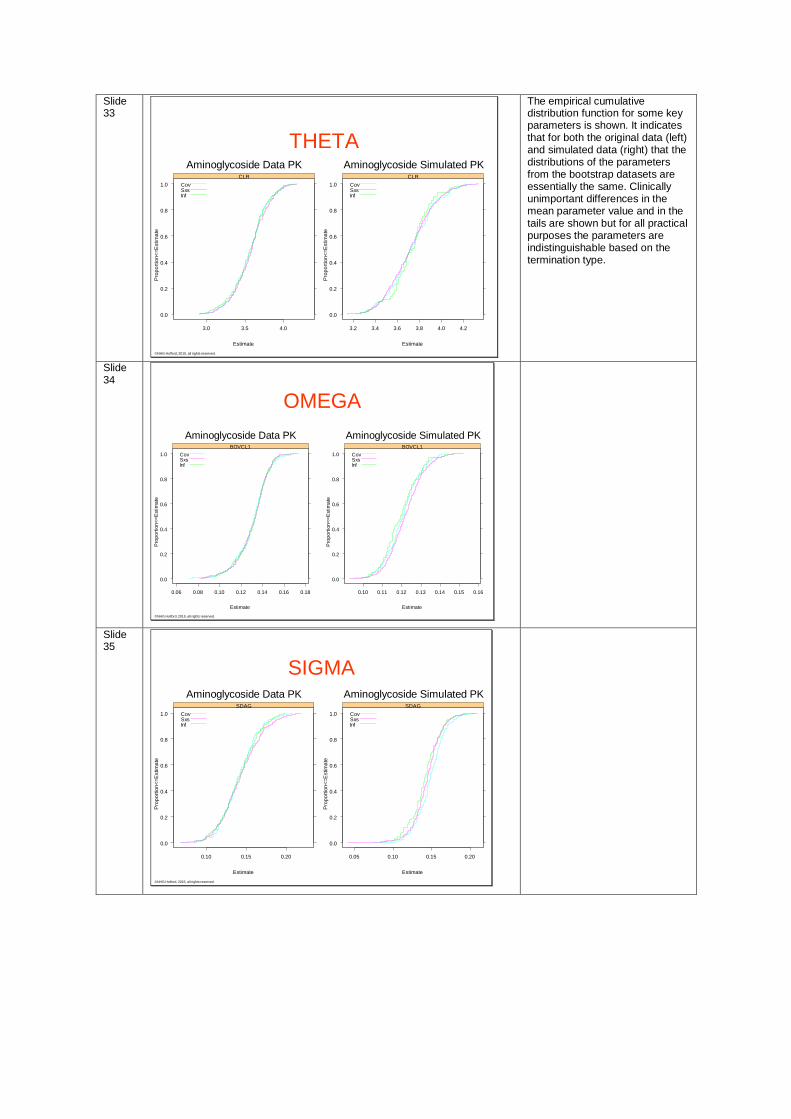
The empirical cumulative distribution function for some key parameters is shown. It indicates that for both the original data (left) and simulated data (right) that the distributions of the parameters from the bootstrap datasets are essentially the same. Clinically unimportant differences in the mean parameter value and in the tails are shown but for all practical purposes the parameters are indistinguishable based on the termination type.

Slide 34


OMEGA

0.0

0.2

0.4

0.6

0.8

1.0

0.06 0.08 0.10 0.12 0.14 0.16 0.18

BOVCL1

Estimate

Pro

po

rtio

n<

=E

stim

ate


CovSxsInf

0.0

0.2

0.4

0.6

0.8

1.0

0.10 0.11 0.12 0.13 0.14 0.15 0.16

BOVCL1

Estimate

Pro

po

rtio

n<

=E

stim

ate


CovSxsInf

Slide 35


SIGMA

0.0

0.2

0.4

0.6

0.8

1.0

0.10 0.15 0.20

SDAG

Estimate

Pro

po

rtio

n<

=E

stim

ate


CovSxsInf

0.0

0.2

0.4

0.6

0.8

1.0

0.05 0.10 0.15 0.20

SDAG

Estimate

Pro

po

rtio

n<

=E

stim

ate


CovSxsInf

Slide 36


$COV Error

$COV/BS StDev -1

COV SXS RND INF

data df THETA -1% 0% 3% 4%

data g77 THETA -6% -5% -5% 2%

sim df THETA -9% -9% -10% -11%

The estimated standard error obtained from the mean of the $COV estimates is compared to the standard deviation of the boostrap estimates. It shows that for all cases the difference is small. The simulated data set tends to have about a 10% underestimate of the true (bootstrap) standard error when it is computed from $COV. This might be expected from the asymptotic properties of the $COV standard error.

Slide 37


Bootstrap 80% Confidence Interval

BSCI: Empirical

» 10%centile to 90%centile

BSSE: Asymptotic Normal Distribution

» 1.28*2 * Bootstrap StDev

BS Asymptotic Error

» (BSSE/BSCI-1)*100

A second comparison is made of the $COV and bootstrap predictions of the 80% confidence interval. The bootstrap CI was obtained from the 10%centile to 90%centile values in the bootstrap distribution. The bootstrap standard error was also used to predict a 80% CI based on the normal distribution assumption.

Slide 38


BS StDev

Normal Distribution Assumption

Error

Stats COV SXS RND INF

THETA -21% -23% -21% -21%

Data df OMEGA -23% -21% -20% -20%

SIGMA -19% -22% -23% -22%

THETA -15% -19% -22% -20%

Data g77 OMEGA -19% -22% -20% -19%

SIGMA -22% -23% -23% -15%

THETA -21% -21% -21% -20%

Sim df OMEGA -21% -17% -21% -22%

SIGMA -21% -21% -21% -20%

Average -20% -21% -21% -20%

The standard error prediction of the 80%CI was consistently about 20% lower than the bootstrap empirical distribution CI. Once again this is compatible with the asymptotic prediction based on using SE.

Slide 39


Conclusions

NONMEM termination status is not a useful predictor of parameter reliability when the final model is acceptable ‘in context’

Compaq compiler is superior to g77 compiler in completing $COV step

$COV slightly underestimates SE

SE prediction of parameter confidence interval underestimates the empirical bootstrap interval

In conclusion, for this specific data set and model it seems that one should not rely on the NONMEM termination type as a measure of parameter reliability. This result may have more generalizable application provided one is confident that the model is a good description of the data and is not stuck at a local minimum (e.g. by comparison with other similar models).

Slide 40


References

Efron B. Bootstrap methods: another look at the jackknife. The Annals of

Statistics 1979;7(1):1-26

Efron B, Tibshirani R. Statistical data analysis in the computer age.

Science 1991;253(5018):390-395

Holford NH, Peace KE. Results and validation of a population

pharmacodynamic model for cognitive effects in Alzheimer patients

treated with tacrine. Proceedings of the National Academy of Sciences of

the United States of America 1992;89(23):11471-11475

Quenouille M. Approximation tests of correlation in time series. Journal of

the Royal Statistical Society B 1949;11:18-84

Stine (annotated bibliography) http://www.icpsr.umich.edu/TRAINING/Biblio95/stine.html

Tukey J. Bias and confidence in not quite large samples. Annals of

Mathematical Statistics 1958;29:614

Documents

Confidence Intervals z Learn and Confirm Cycle …holford.fmhs.auckland.ac.nz/.../bootstrap-and-confidence-intervals.pdf · » Confidence intervals are often asymmetric The standard