Embed Size (px)
Citation preview

Chapter 6
Confidence Intervals
1
Chapter Outline
• 6.1 Confidence Intervals for the Mean (Large Samples)
• 6.2 Confidence Intervals for the Mean (Small Samples)
• 6.3 Confidence Intervals for Population Proportions
• 6.4 Confidence Intervals for Variance and Standard Deviation
2
Section 6.1
Confidence Intervals for the Mean (Large Samples)
3
Section 6.1 Objectives
• Find a point estimate and a margin of error
• Construct and interpret confidence intervals for the population mean
• Determine the minimum sample size required when estimating μ
4
Point Estimate for Population μ
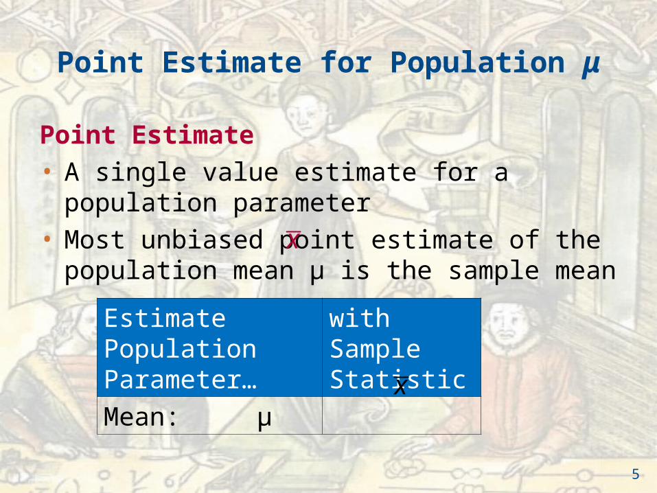
Point Estimate
• A single value estimate for a population parameter
• Most unbiased point estimate of the population mean μ is the sample mean x
Estimate Population Parameter…
with Sample Statistic
Mean: μ x
5
Example: Point Estimate for Population μ
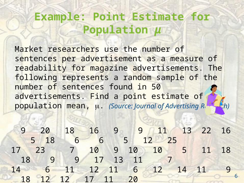
Market researchers use the number of sentences per advertisement as a measure of readability for magazine advertisements. The following represents a random sample of the number of sentences found in 50 advertisements. Find a point estimate of the population mean, . (Source: Journal of Advertising Research)
9 20 18 16 9 9 11 13 22 16 5 18 6 6 5 12 2517 23 7 10 9 10 10 5 11 18 18 9 9 17 13 11 714 6 11 12 11 6 12 14 11 9 18 12 12 17 11 20
6
Solution: Point Estimate for Population μ
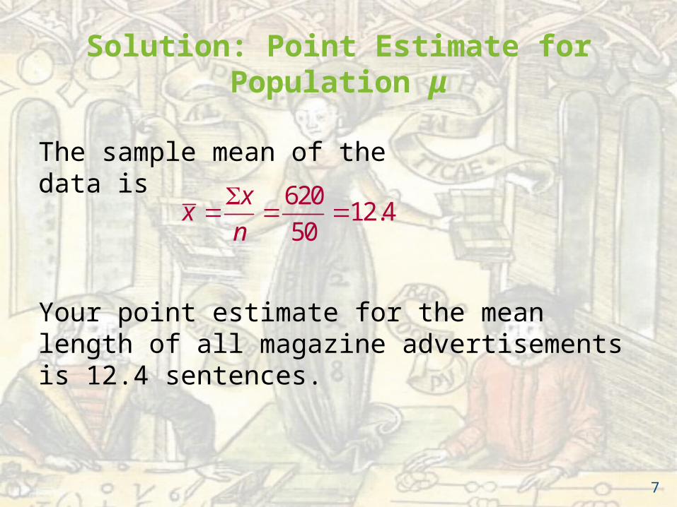
The sample mean of the data is
62012.4
50
xx
n
Your point estimate for the mean length of all magazine advertisements is 12.4 sentences.
7
Interval Estimate
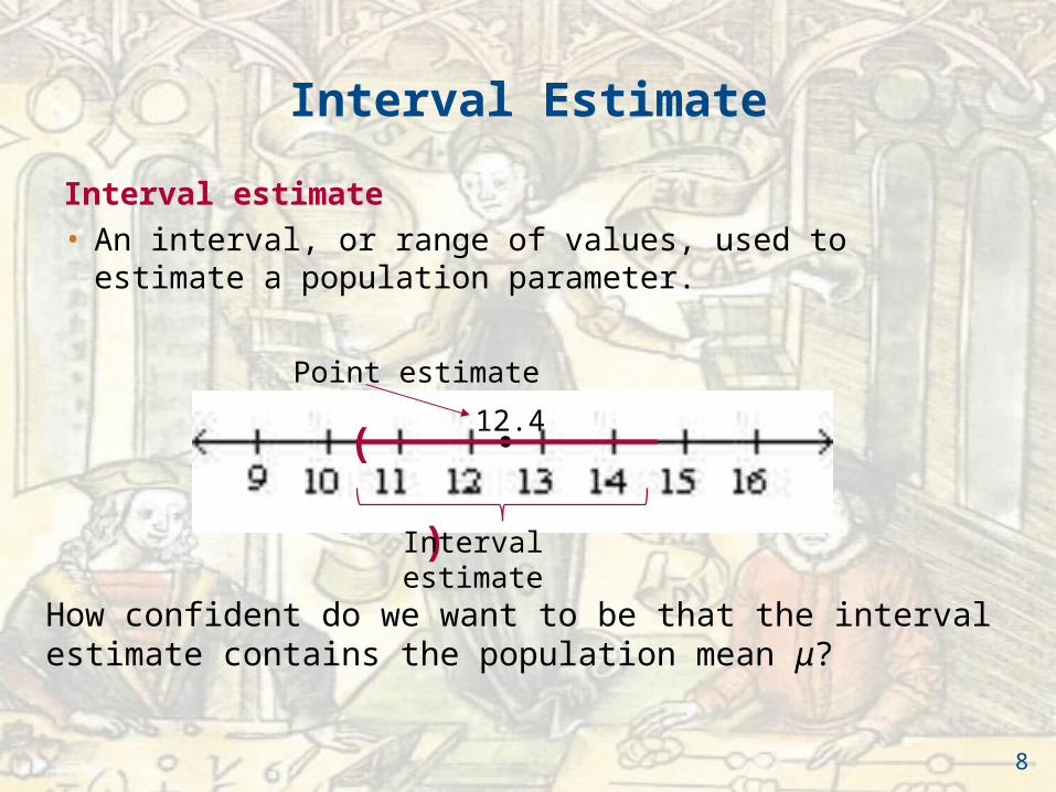
Interval estimate
• An interval, or range of values, used to estimate a population parameter.
Point estimate
• 12.4
How confident do we want to be that the interval estimate contains the population mean μ?
( )
Interval estimate
8
Level of Confidence
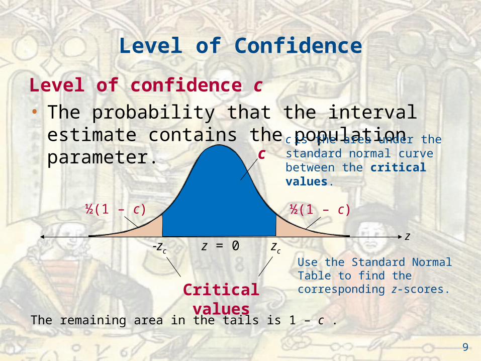
Level of confidence c
• The probability that the interval estimate contains the population parameter.
zz = 0-zc zc
Critical values
½(1 – c) ½(1 – c)
c is the area under the standard normal curve between the critical values.
The remaining area in the tails is 1 – c .
c
Use the Standard Normal Table to find the corresponding z-scores.
9
zc
Level of Confidence
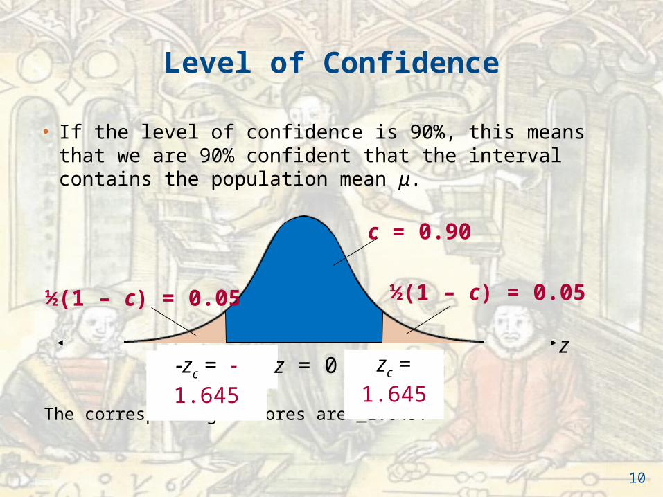
• If the level of confidence is 90%, this means that we are 90% confident that the interval contains the population mean μ.
zz = 0 zc
The corresponding z-scores are +1.645.
c = 0.90
½(1 – c) = 0.05½(1 – c) = 0.05
-zc = -1.645 zc = 1.645
10
Sampling Error
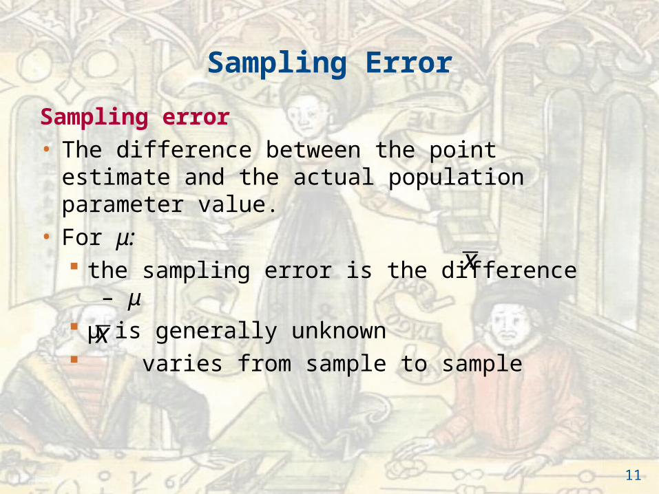
Sampling error
• The difference between the point estimate and the actual population parameter value.
• For μ: the sampling error is the difference – μ μ is generally unknown varies from sample to sample
x
x
11
Margin of Error
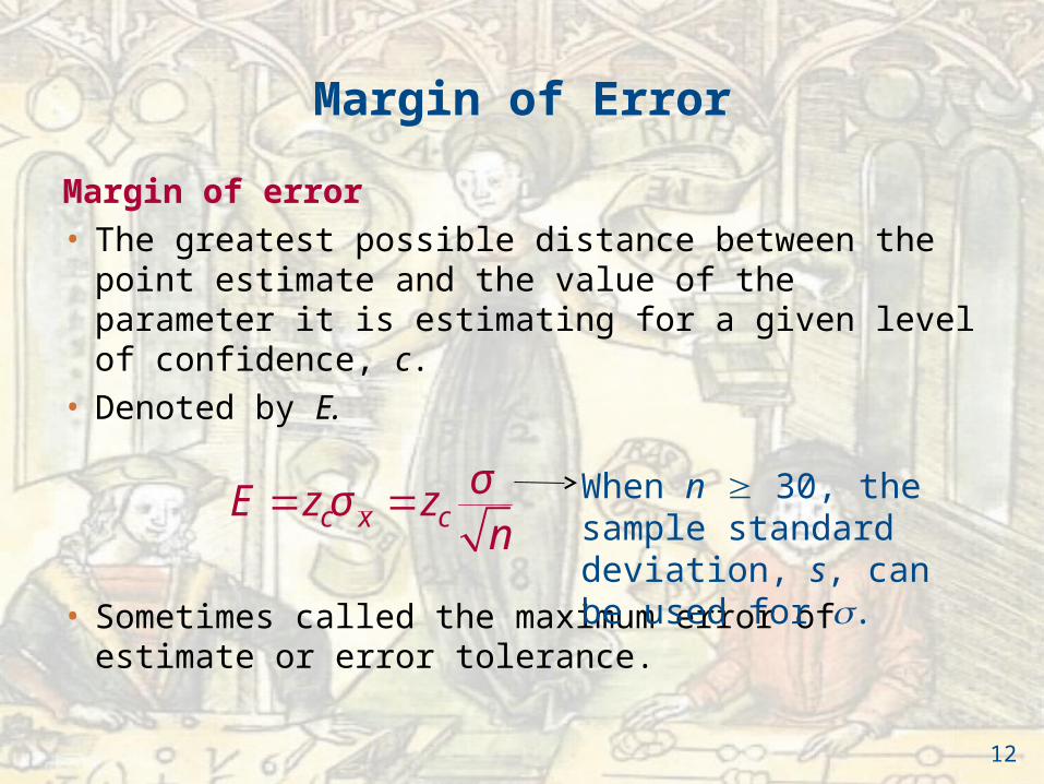
Margin of error
• The greatest possible distance between the point estimate and the value of the parameter it is estimating for a given level of confidence, c.
• Denoted by E.
• Sometimes called the maximum error of estimate or error tolerance.
c x cE z zn
σσ When n 30, the sample standard deviation, s, can be used for .
12
Example: Finding the Margin of Error
Use the magazine advertisement data and a 95% confidence level to find the margin of error for the mean number of sentences in all magazine advertisements. Assume the sample standard deviation is about 5.0.
13
zc
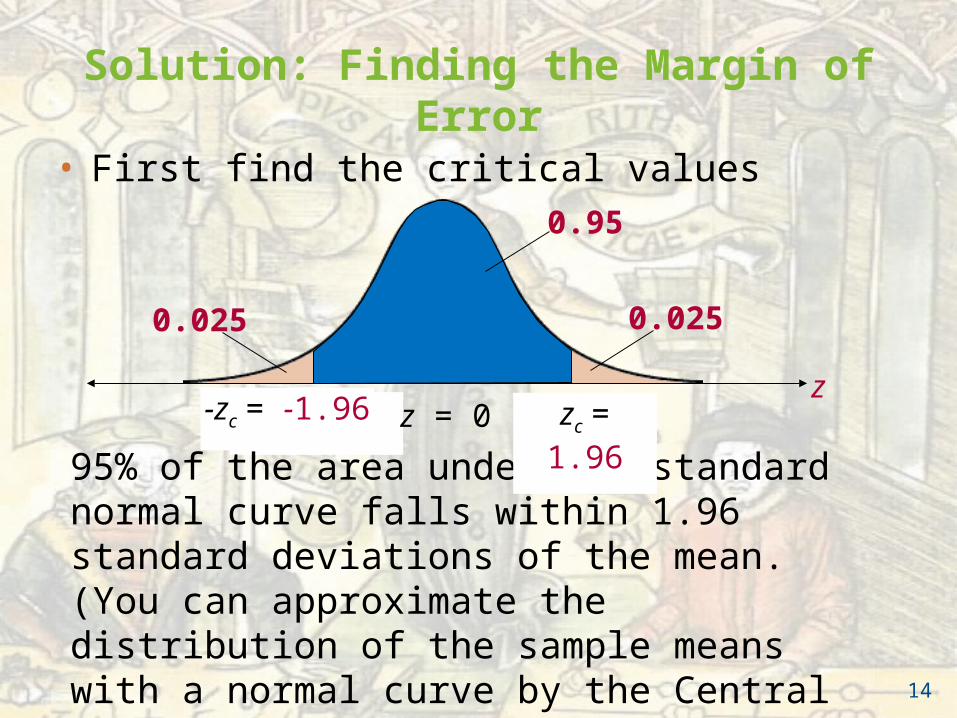
Solution: Finding the Margin of Error
• First find the critical values
zzcz = 0
0.95
0.0250.025
-zc = -1.96
95% of the area under the standard normal curve falls within 1.96 standard deviations of the mean. (You can approximate the distribution of the sample means with a normal curve by the Central Limit Theorem, because n ≥ 30.)
14
zc = 1.96
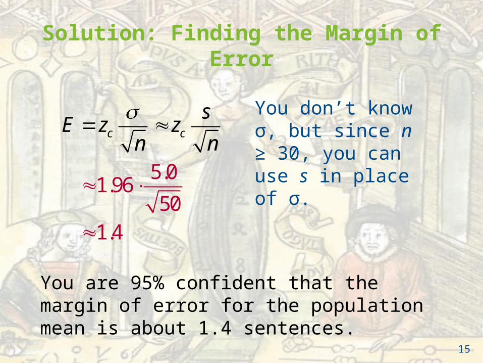
Solution: Finding the Margin of Error
5.01.96
501.4
c c
sE z z
n n
You don’t know σ, but since n ≥ 30, you can use s in place of σ.
You are 95% confident that the margin of error for the population mean is about 1.4 sentences.
15
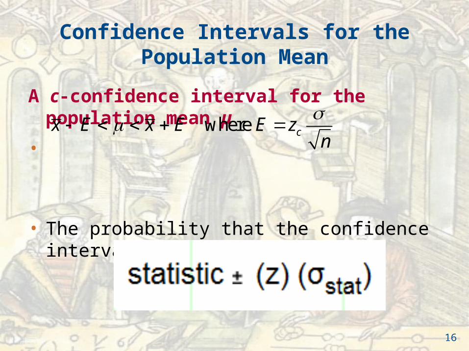
Confidence Intervals for the Population Mean
A c-confidence interval for the population mean μ
•
• The probability that the confidence interval contains μ is c.
where cx E x E E zn
16
Constructing Confidence Intervals for μ
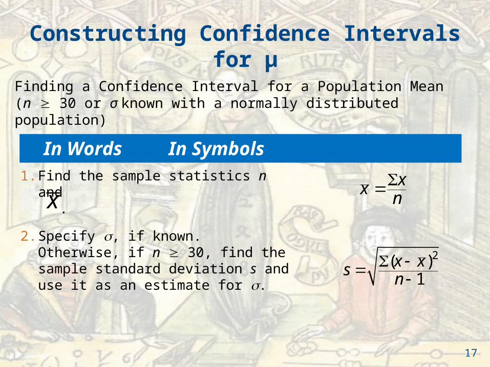
Finding a Confidence Interval for a Population Mean (n 30 or σ known with a normally distributed population)
In Words In Symbols
1. Find the sample statistics n and .
2. Specify , if known. Otherwise, if n 30, find the sample standard deviation s and use it as an estimate for .
xxn
2( )1
x xsn
x
17
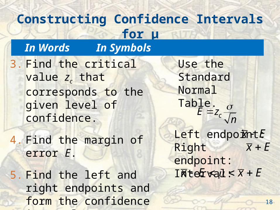
Constructing Confidence Intervals for μ
3. Find the critical value zc that corresponds to the given level of confidence.
4. Find the margin of error E.
5. Find the left and right endpoints and form the confidence interval.
Use the Standard Normal Table.
Left endpoint: Right endpoint: Interval:
cE zn
x Ex E
x E x E
18
In Words In Symbols
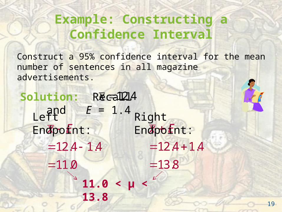
Example: Constructing a Confidence Interval
Construct a 95% confidence interval for the mean number of sentences in all magazine advertisements.
Solution: Recall and E = 1.412.4x
12.4 1.4
11.0
x E
12.4 1.4
13.8
x E
11.0 < μ < 13.8
Left Endpoint: Right Endpoint:
19
( )
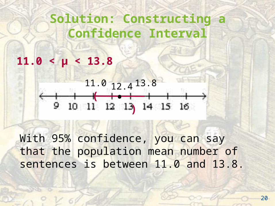
Solution: Constructing a Confidence Interval
11.0 < μ < 13.8
• 12.411.0 13.8
With 95% confidence, you can say that the population mean number of sentences is between 11.0 and 13.8.
20

Example: Constructing a Confidence Interval σ Known
A college admissions director wishes to estimate the mean age of all students currently enrolled. In a random sample of 20 students, the mean age is found to be 22.9 years. From past studies, the standard deviation is known to be 1.5 years, and the population is normally distributed. Construct a 90% confidence interval of the population mean age.
21
zc
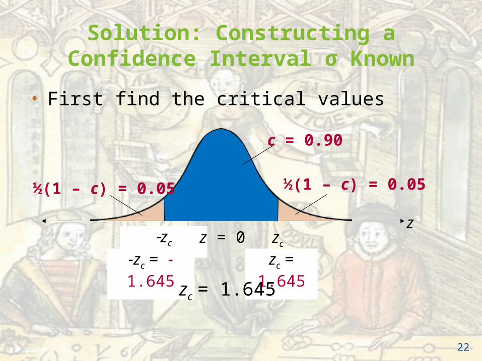
Solution: Constructing a Confidence Interval σ Known
• First find the critical values
zz = 0 zc
c = 0.90
½(1 – c) = 0.05½(1 – c) = 0.05
-zc = -1.645 zc = 1.645
zc = 1.645
22
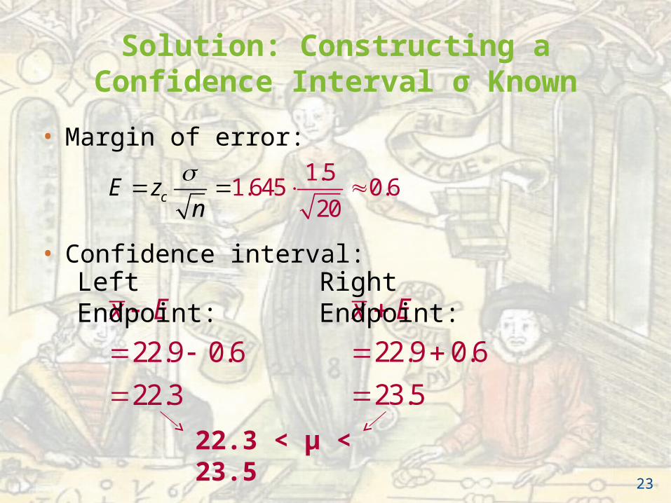
• Margin of error:
• Confidence interval:
Solution: Constructing a Confidence Interval σ Known
1.51.645 0.6
20cE z
n
22.9 0.6
22.3
x E
22.9 0.6
23.5
x E
Left Endpoint: Right Endpoint:
22.3 < μ < 23.5
23
Solution: Constructing a Confidence Interval σ Known
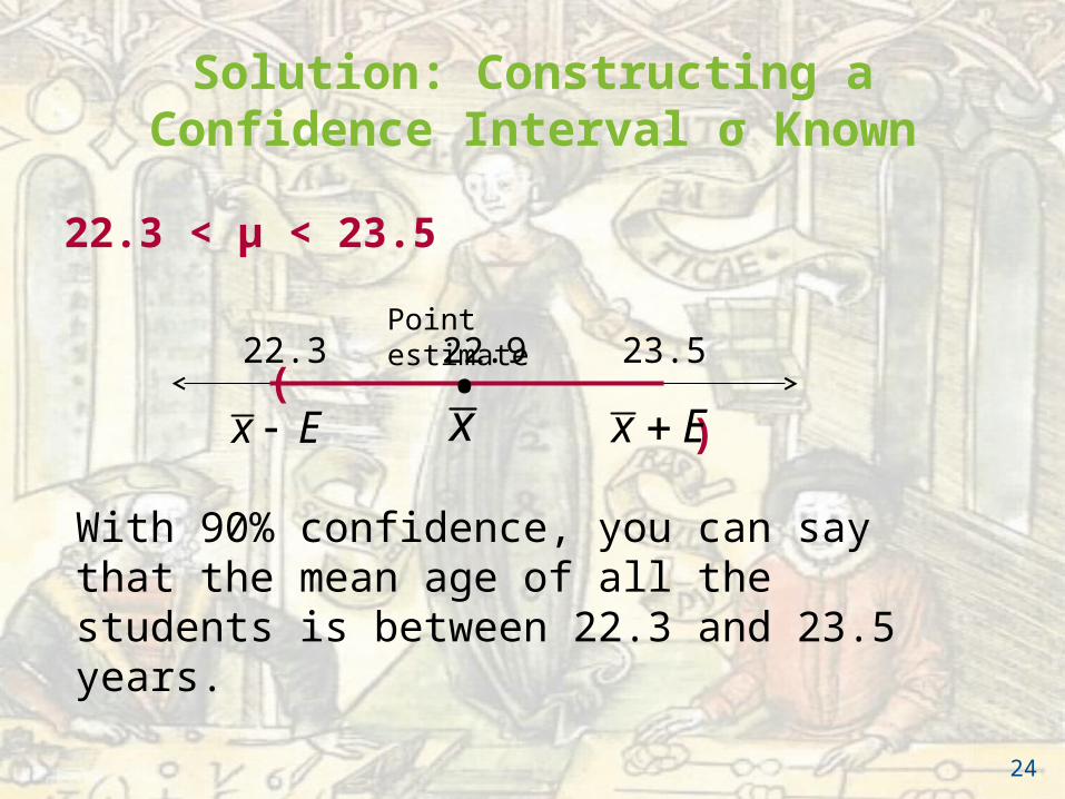
22.3 < μ < 23.5
( )• 22.922.3 23.5
With 90% confidence, you can say that the mean age of all the students is between 22.3 and 23.5 years.
Point estimate
xx E x E
24
Slide 6- 25
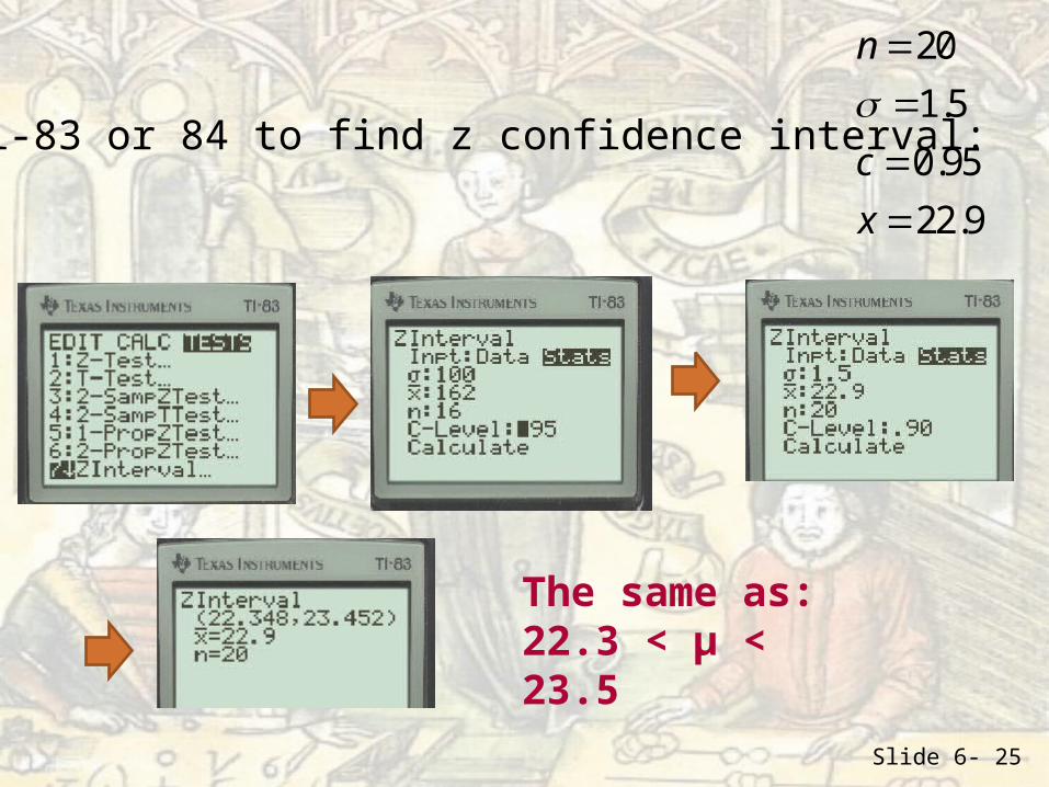
20
1.5
0.95
22.9
n
c
x
Using Ti-83 or 84 to find z confidence interval:
The same as:22.3 < μ < 23.5
Interpreting the Results
• μ is a fixed number. It is either in the confidence interval or not.
• Incorrect: “There is a 90% probability that the actual mean is in the interval (22.3, 23.5).”
• Correct: “If a large number of samples is collected and a confidence interval is created for each sample, approximately 90% of these intervals will contain μ.
26

Slide 6- 27
Confidence Intervals
http://www.learner.org/courses/againstallodds/unitpages/unit24.html
Interpreting the Results
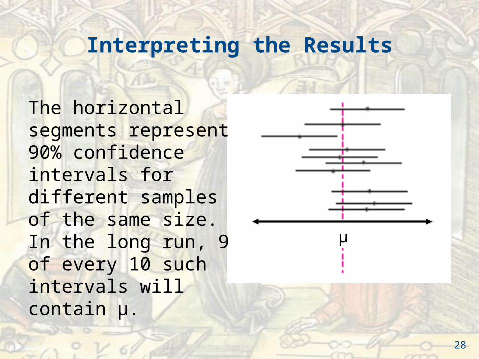
The horizontal segments represent 90% confidence intervals for different samples of the same size.In the long run, 9 of every 10 such intervals will contain μ.
28
μ
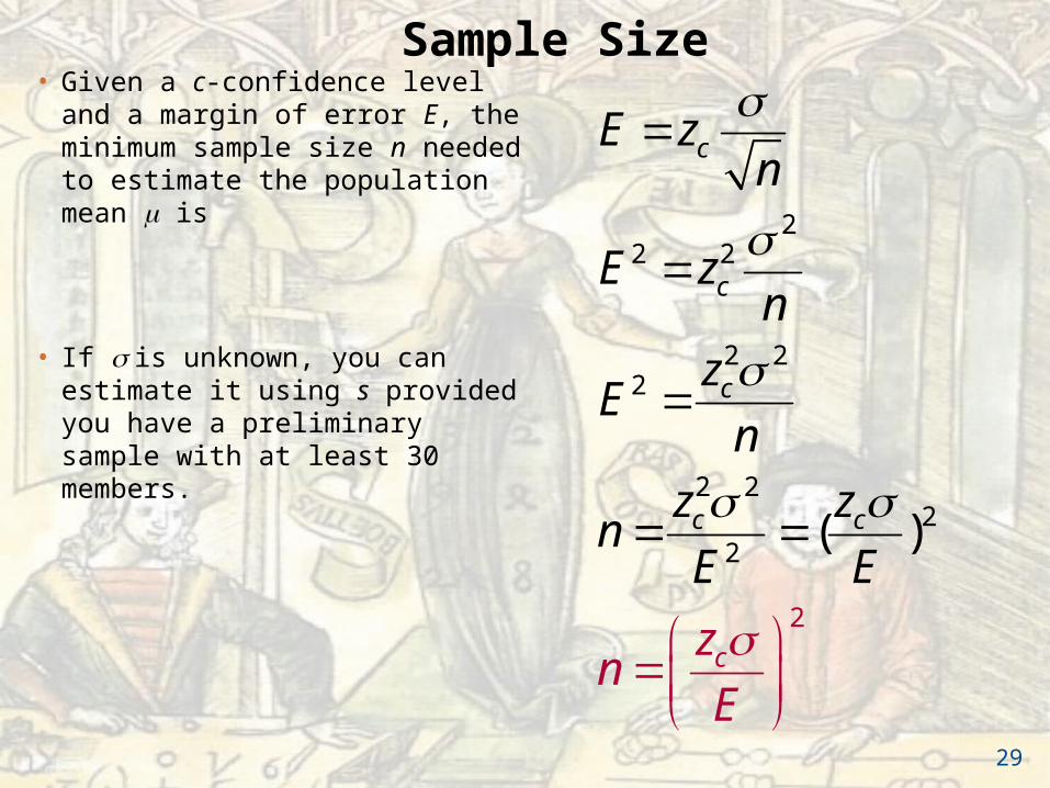
• Given a c-confidence level and a margin of error E, the minimum sample size n needed to estimate the population mean is
• If is unknown, you can estimate it using s provided you have a preliminary sample with at least 30 members.
22 2
2 22
2 22
2
2
( )
c
c
c
c
c
c
E zn
E zn
zE
n
z z
zn
E
nE E
29
Sample Size
Example: Sample Size
You want to estimate the mean number of sentences in a magazine advertisement. How many magazine advertisements must be included in the sample if you want to be 95% confident that the sample mean is within one sentence of the population mean? Assume the sample standard deviation is about 5.0.
30
zc
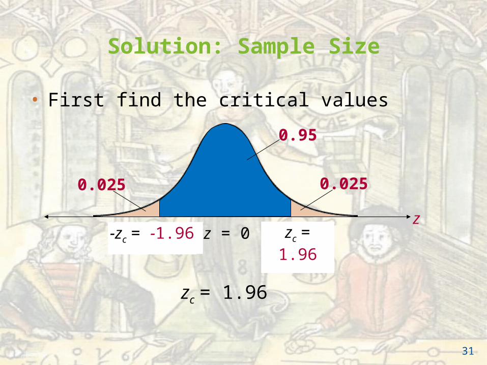
Solution: Sample Size
• First find the critical values
zc = 1.96
zz = 0 zc
0.95
0.0250.025
-zc = -1.96
31
zc = 1.96

Solution: Sample Size
zc = 1.96 s = 5.0 E = 1
221.96 5.0
96.041
czn
E
When necessary, round up to obtain a whole number.
You should include at least 97 magazine advertisements in your sample.
32
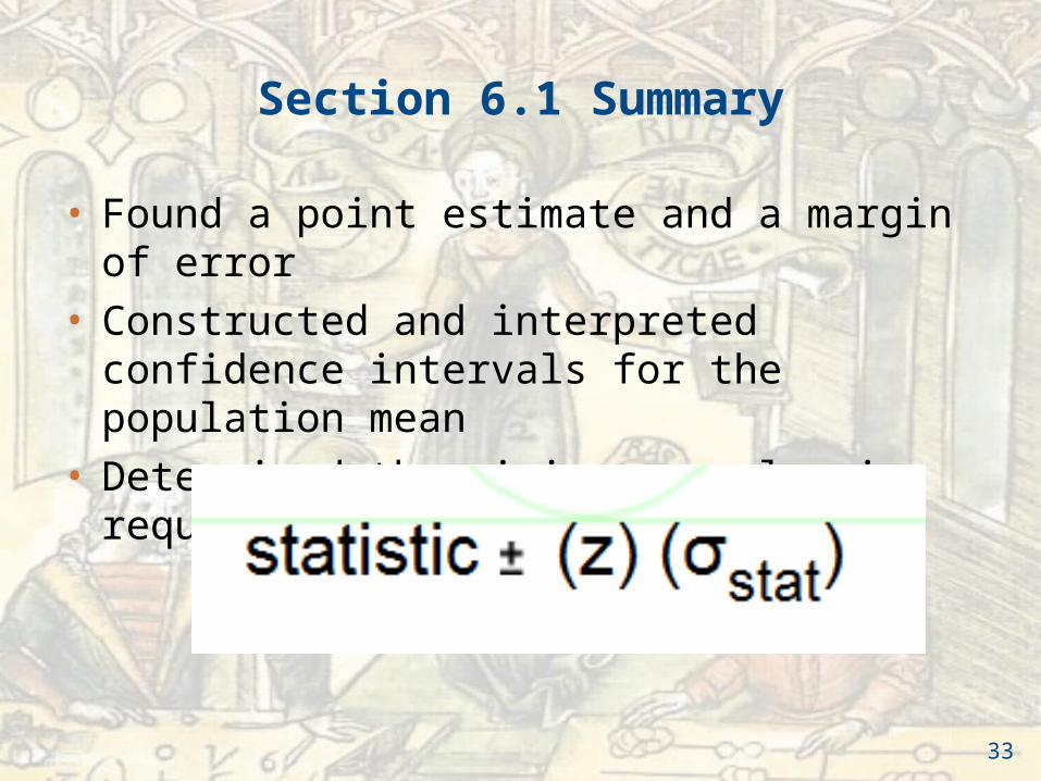
Section 6.1 Summary
• Found a point estimate and a margin of error
• Constructed and interpreted confidence intervals for the population mean
• Determined the minimum sample size required when estimating μ
33
Section 6.2
Confidence Intervals for the Mean (Small Samples)
34
Section 6.2 Objectives
• Interpret the t-distribution and use a t-distribution table
• Construct confidence intervals when n < 30, the population is normally distributed, and σ is unknown
35
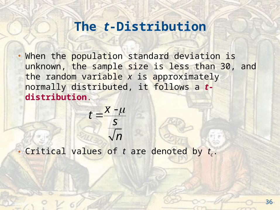
The t-Distribution
• When the population standard deviation is unknown, the sample size is less than 30, and the random variable x is approximately normally distributed, it follows a t-distribution.
• Critical values of t are denoted by tc.
-xtsn
36
Slide 6- 37
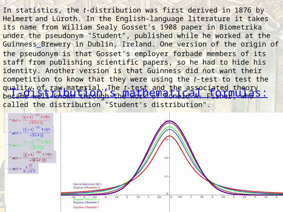
In statistics, the t-distribution was first derived in 1876 by Helmert and Lüroth. In the English-language literature it takes its name from William Sealy Gosset's 1908 paper in Biometrika under the pseudonym "Student", published while he worked at the Guinness Brewery in Dublin, Ireland. One version of the origin of the pseudonym is that Gosset's employer forbade members of its staff from publishing scientific papers, so he had to hide his identity. Another version is that Guinness did not want their competition to know that they were using the t-test to test the quality of raw material. The t-test and the associated theory became well-known through the work of Ronald A. Fisher, who called the distribution "Student's distribution".
T-distribution’s mathematical formulas:
Properties of the t-Distribution
1. The t-distribution is bell shaped and symmetric about the mean.
2. The t-distribution is a family of curves, each determined by a parameter called the degrees of freedom. The degrees of freedom are the number of free choices left after a sample statistic such as is calculated. When you use a t-distribution to estimate a population mean, the degrees of freedom are equal to one less than the sample size. d.f. = n – 1 Degrees of freedom
x
38
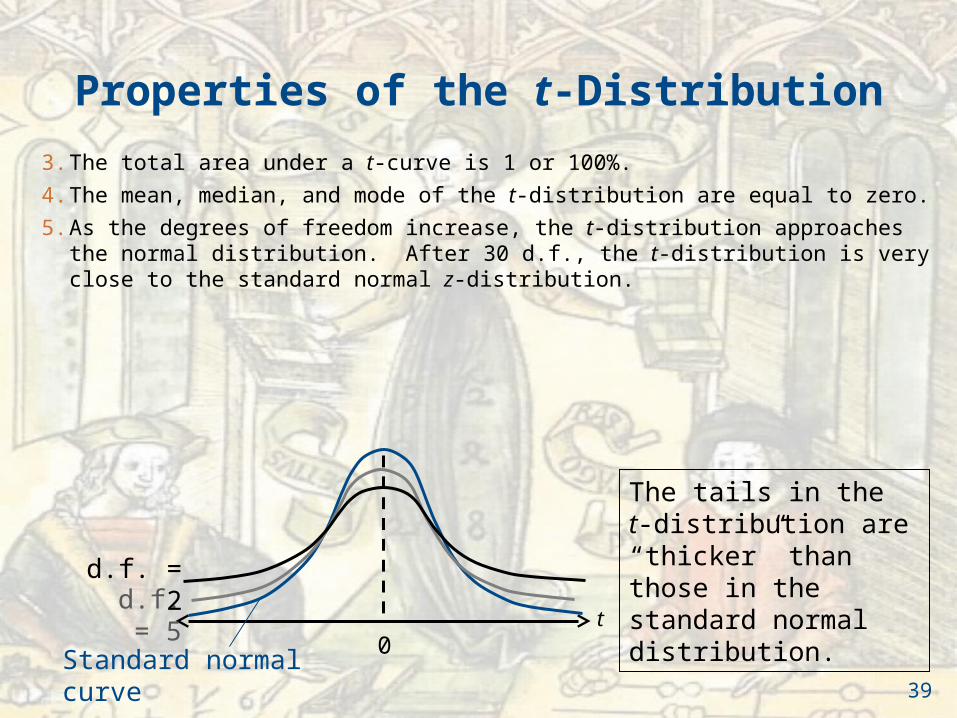
Properties of the t-Distribution
3. The total area under a t-curve is 1 or 100%.
4. The mean, median, and mode of the t-distribution are equal to zero.
5. As the degrees of freedom increase, the t-distribution approaches the normal distribution. After 30 d.f., the t-distribution is very close to the standard normal z-distribution.
t0
Standard normal curve
The tails in the t-distribution are “thicker” than those in the standard normal distribution.d.f. = 5
d.f. = 2
39
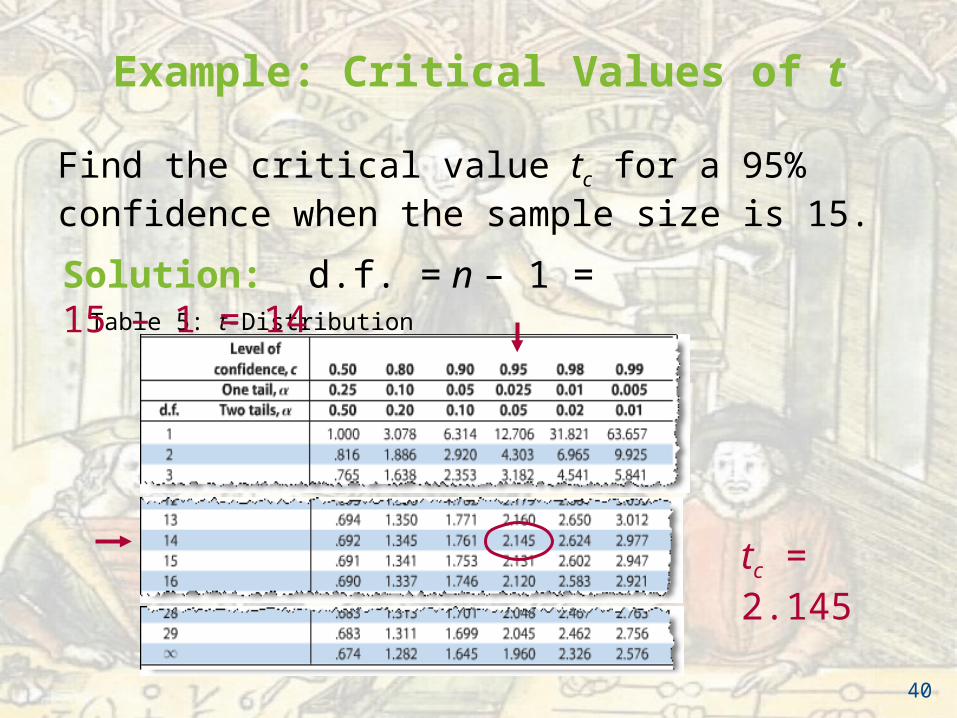
Example: Critical Values of t
Find the critical value tc for a 95% confidence when the sample size is 15.
Table 5: t-Distribution
tc = 2.145
Solution: d.f. = n – 1 = 15 – 1 = 14
40
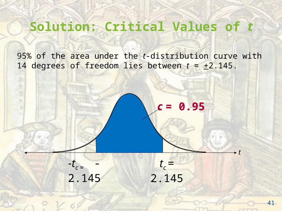
Solution: Critical Values of t
95% of the area under the t-distribution curve with 14 degrees of freedom lies between t = +2.145.
t
-tc = -2.145 tc = 2.145
c = 0.95
41
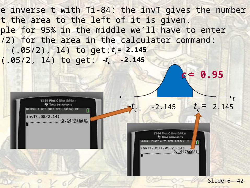
Slide 6- 42
Using the inverse t with Ti-84: the invT gives the number such that the area to the left of it is given.For example for 95% in the middle we’ll have to enter.95+(.05/2) for the area in the calculator command:invT(.95 +(.05/2), 14) to get:and invT(.05/2, 14) to get:
t-tc = -2.145 tc = 2.145
c = 0.95
tc = 2.145
-tc = -2.145
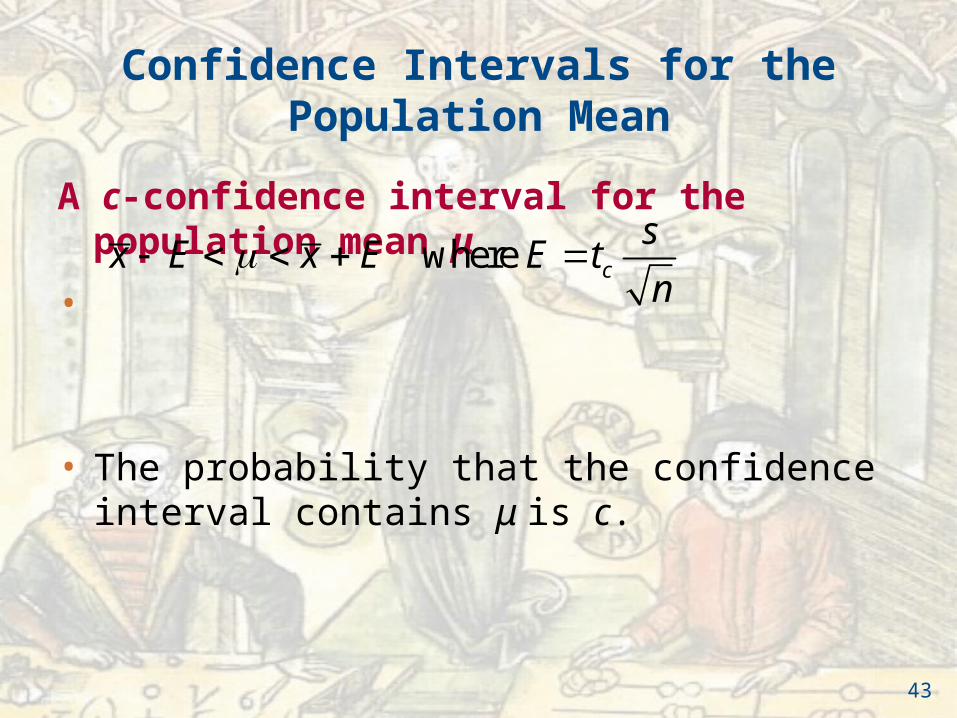
Confidence Intervals for the Population Mean
A c-confidence interval for the population mean μ
•
• The probability that the confidence interval contains μ is c.
where c
sx E x E E t
n
43
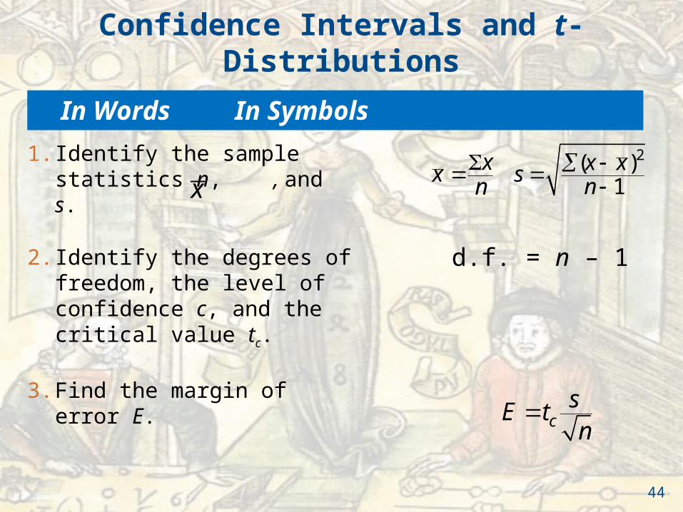
Confidence Intervals and t-Distributions
1. Identify the sample statistics n, , and s.
2. Identify the degrees of freedom, the level of confidence c, and the critical value tc.
3. Find the margin of error E.
xxn
2( )1
x xsn
cE tn
s
d.f. = n – 1
x
44
In Words In Symbols
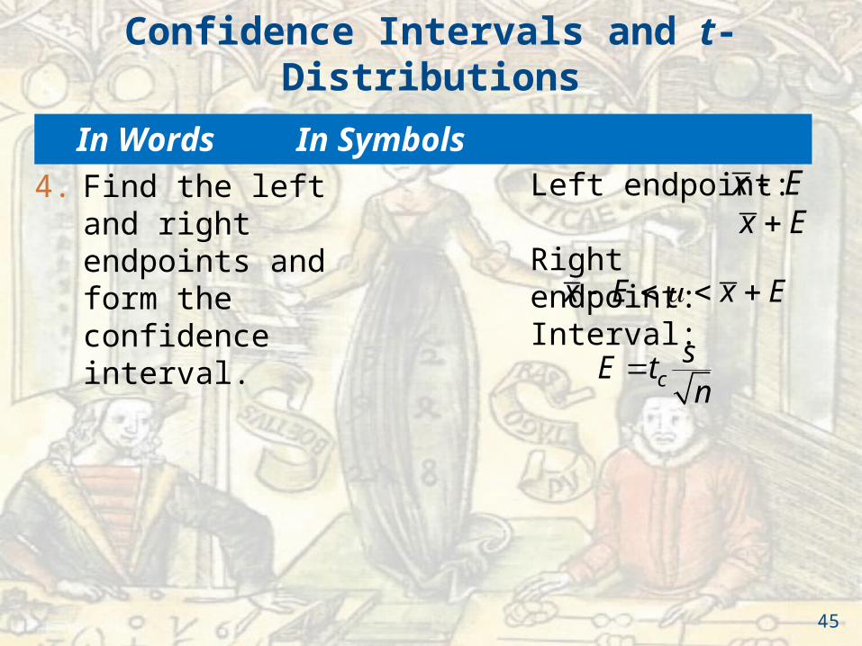
Confidence Intervals and t-Distributions
4. Find the left and right endpoints and form the confidence interval.
Left endpoint: Right endpoint: Interval:
x Ex E
x E x E
45
In Words In Symbols
cE tn
s
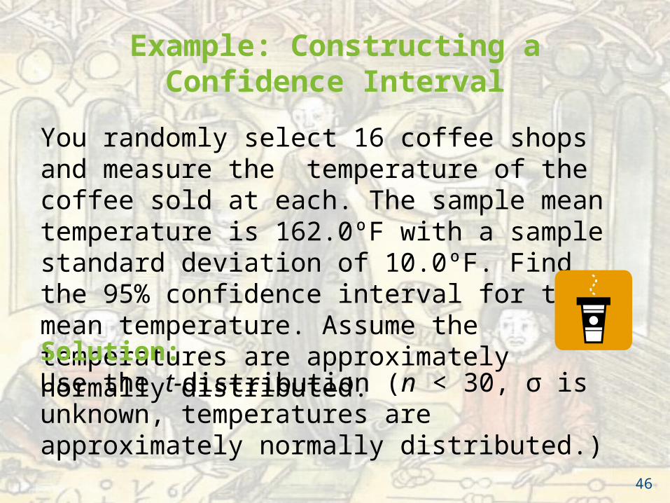
Example: Constructing a Confidence Interval
You randomly select 16 coffee shops and measure the temperature of the coffee sold at each. The sample mean temperature is 162.0ºF with a sample standard deviation of 10.0ºF. Find the 95% confidence interval for the mean temperature. Assume the temperatures are approximately normally distributed.
Solution:Use the t-distribution (n < 30, σ is unknown, temperatures are approximately normally distributed.)
46
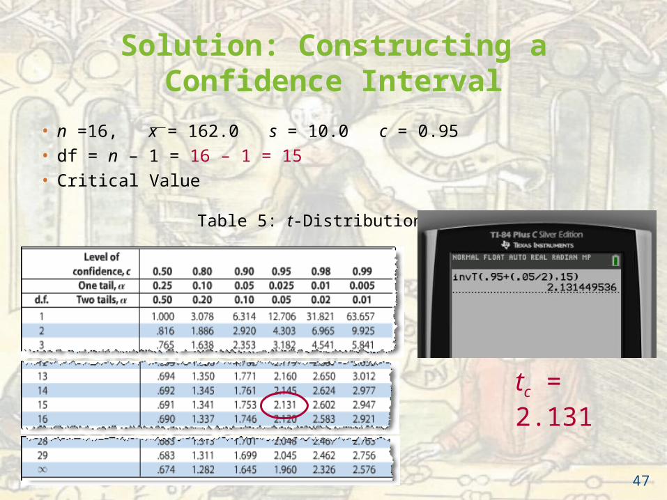
Solution: Constructing a Confidence Interval
• n =16, x = 162.0 s = 10.0 c = 0.95
• df = n – 1 = 16 – 1 = 15
• Critical Value
Table 5: t-Distribution
tc = 2.131
47
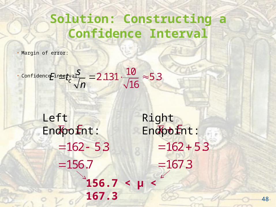
Solution: Constructing a Confidence Interval
• Margin of error:
• Confidence interval:102.131 5.316cE t
n s
162 5.3
156.7
x E
162 5.3
167.3
x E
Left Endpoint: Right Endpoint:
156.7 < μ < 167.3
48
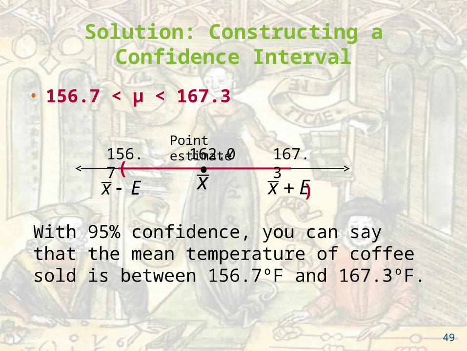
Solution: Constructing a Confidence Interval
• 156.7 < μ < 167.3
( )• 162.0156.7 167.3
With 95% confidence, you can say that the mean temperature of coffee sold is between 156.7ºF and 167.3ºF.
Point estimate
xx E x E
49
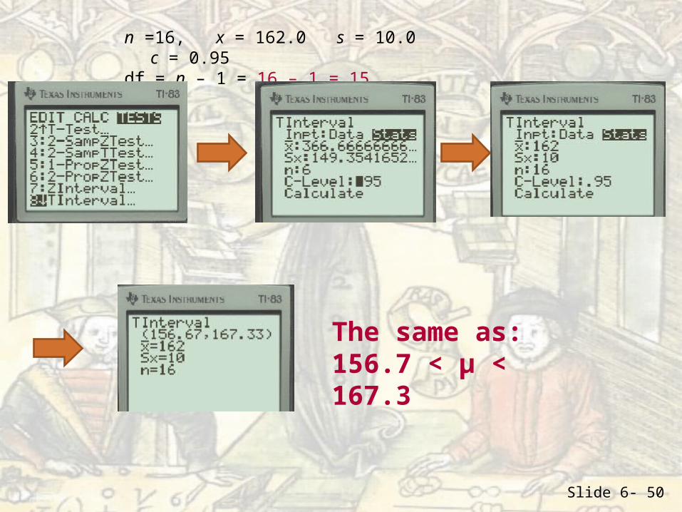
Slide 6- 50
n =16, x = 162.0 s = 10.0 c = 0.95df = n – 1 = 16 – 1 = 15
The same as:156.7 < μ < 167.3
No
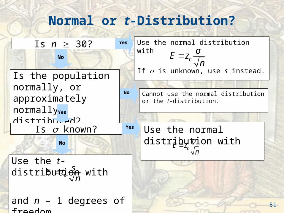
Normal or t-Distribution?
Is n 30?
Is the population normally, or approximately normally, distributed? Cannot use the normal
distribution or the t-distribution. Yes
Is known?No
Use the normal distribution with
If is unknown, use s instead.
cE zn
σYes
No
Use the normal distribution with
cE zn
σ
Yes
Use the t-distribution with
and n – 1 degrees of freedom.
cE tn
s
51
Example: Normal or t-Distribution?
You randomly select 25 newly constructed houses. The sample mean construction cost is $181,000 and the population standard deviation is $28,000. Assuming construction costs are normally distributed, should you use the normal distribution, the t-distribution, or neither to construct a 95% confidence interval for the population mean construction cost?
Solution:Use the normal distribution (the population is normally distributed and the population standard deviation is known)
52
Section 6.2 Summary
• Interpreted the t-distribution and used a t-distribution table
• Constructed confidence intervals when n < 30, the population is normally distributed, and σ is unknown
53
Section 6.3
Confidence Intervals for Population Proportions
54
Section 6.3 Objectives
• Find a point estimate for the population proportion
• Construct a confidence interval for a population proportion
• Determine the minimum sample size required when estimating a population proportion
55
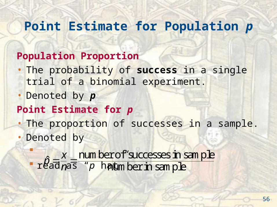
Point Estimate for Population p
Population Proportion
• The probability of success in a single trial of a binomial experiment.
• Denoted by p
Point Estimate for p
• The proportion of successes in a sample.
• Denoted by read as “p hat”
number of successes in sampleˆ number in samplexpn
56
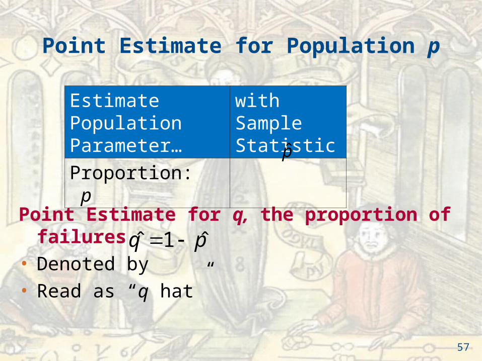
Point Estimate for Population p
Point Estimate for q, the proportion of failures
• Denoted by
• Read as “q hat”
1ˆ ˆq p
Estimate Population Parameter…
with Sample Statistic
Proportion: p p̂
57
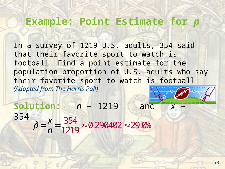
Example: Point Estimate for p
In a survey of 1219 U.S. adults, 354 said that their favorite sport to watch is football. Find a point estimate for the population proportion of U.S. adults who say their favorite sport to watch is football. (Adapted from The Harris Poll)
Solution: n = 1219 and x = 354
354 0.29ˆ 0402 29.0%1219
xpn
58
ˆ
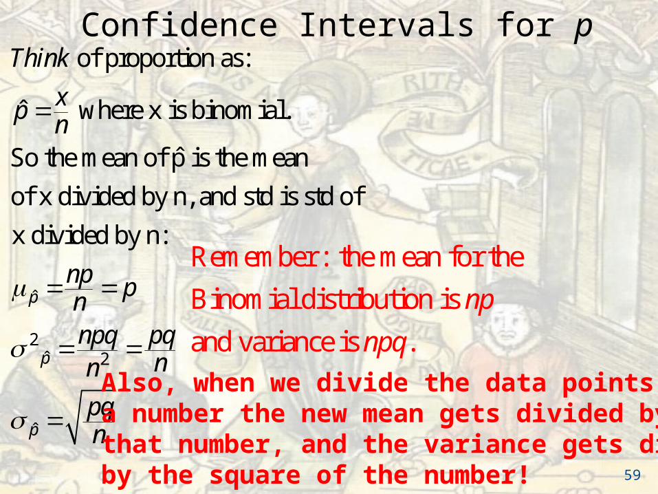
2ˆ 2
ˆ
of proportion as:
where x is binomial.ˆ
So the mean of p̂ is the mean
of x divided by n, and std is std of
x divided by n:
p
p
p
Think
xpn
np pnnpq pq
nn
pqn
59
Confidence Intervals for p
Remember : the mean for the
Binomial distribution is
and variance is .
np
npq
Also, when we divide the data points bya number the new mean gets divided by that number, and the variance gets dividedby the square of the number!
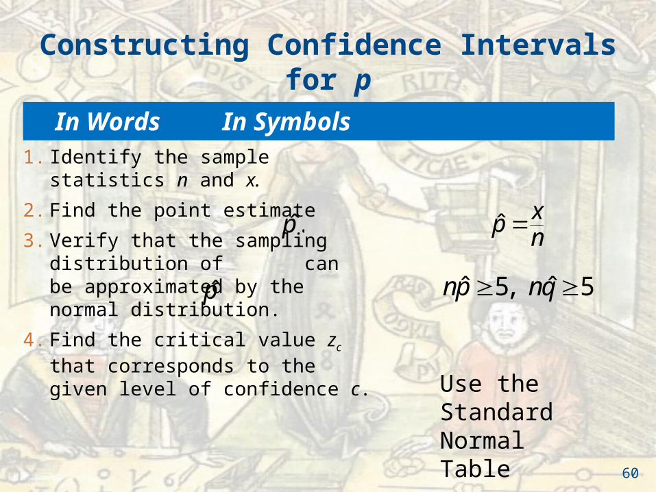
Constructing Confidence Intervals for p
1. Identify the sample statistics n and x.
2. Find the point estimate
3. Verify that the sampling distribution of can be approximated by the normal distribution.
4. Find the critical value zc that corresponds to the given level of confidence c.
ˆ xpn
Use the Standard Normal Table
.̂p
5, 5ˆ ˆnp nq p̂
60
In Words In Symbols
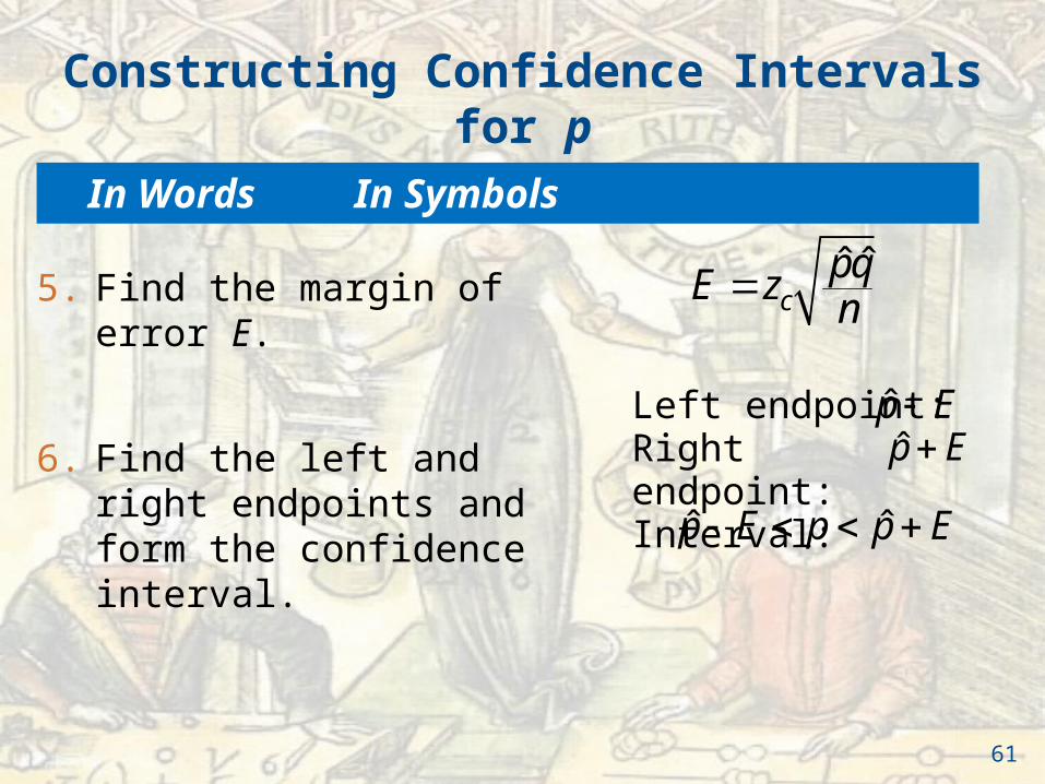
Constructing Confidence Intervals for p
5. Find the margin of error E.
6. Find the left and right endpoints and form the confidence interval.
ˆ ˆc
pqE zn
Left endpoint: Right endpoint: Interval:
p̂ Ep̂ E
ˆ ˆp E p p E
61
In Words In Symbols

Example: Confidence Interval for p
In a survey of 1219 U.S. adults, 354 said that their favorite sport to watch is football. Construct a 95% confidence interval for the proportion of adults in the United States who say that their favorite sport to watch is football.
Solution: Recall ˆ 0.290402p
1 0.290402ˆ ˆ 0.7095981q p
62
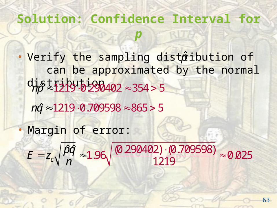
Solution: Confidence Interval for p
• Verify the sampling distribution of can be approximated by the normal distribution
p̂
1219 0.290402 354 5ˆnp
1219 0.709598 865 5ˆnq
• Margin of error:
(0.290402) (0.709598)1.96ˆ ˆ 0.0251219c
pqE zn
63
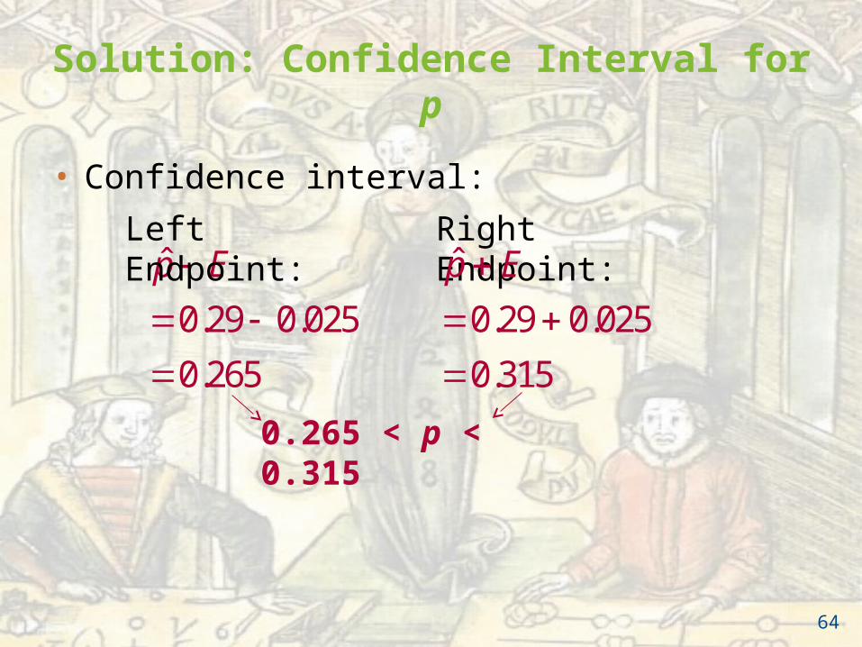
Solution: Confidence Interval for p
• Confidence interval:
ˆ
0.29 0.025
0.265
p E
Left Endpoint: Right Endpoint:
0.265 < p < 0.315
ˆ
0.29 0.025
0.315
p E
64
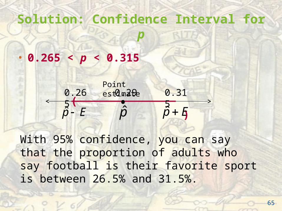
Solution: Confidence Interval for p
• 0.265 < p < 0.315
( )• 0.290.265 0.315
With 95% confidence, you can say that the proportion of adults who say football is their favorite sport is between 26.5% and 31.5%.
Point estimate
p̂p̂ E p̂ E
65
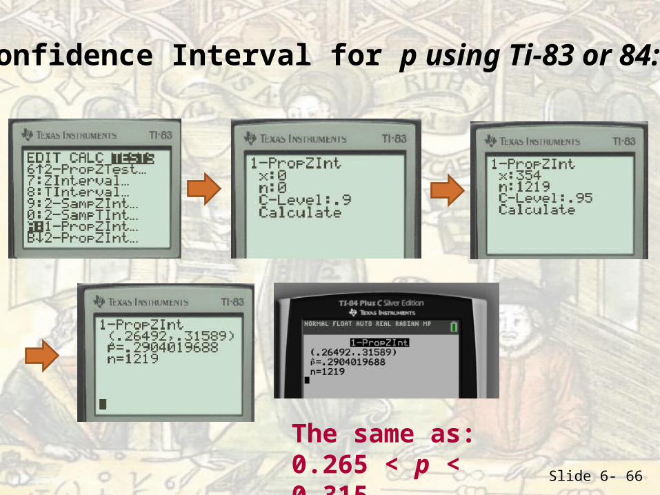
Slide 6- 66
Confidence Interval for p using Ti-83 or 84:
The same as:0.265 < p < 0.315
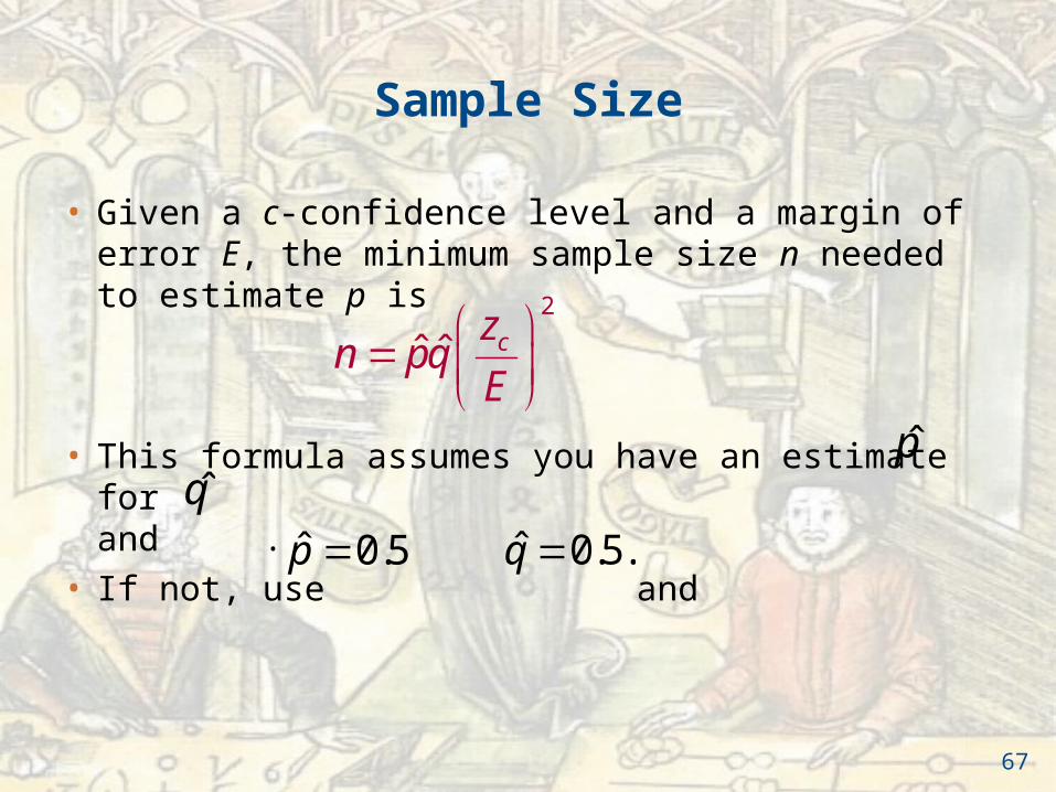
Sample Size
• Given a c-confidence level and a margin of error E, the minimum sample size n needed to estimate p is
• This formula assumes you have an estimate for and .
• If not, use and
2
ˆ ˆ czn pq
E
ˆ 0.5.qˆ 0.5p
p̂q̂
67
Slide 6- 68
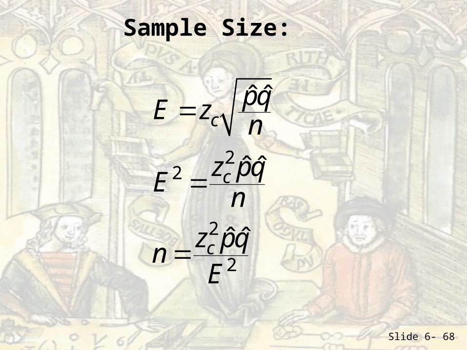
22
2
2
ˆ ˆ
ˆ ˆ
ˆ ˆ
c
c
c
pqE zn
z pqE
n
z pqn
E
Sample Size:
Slide 6- 69
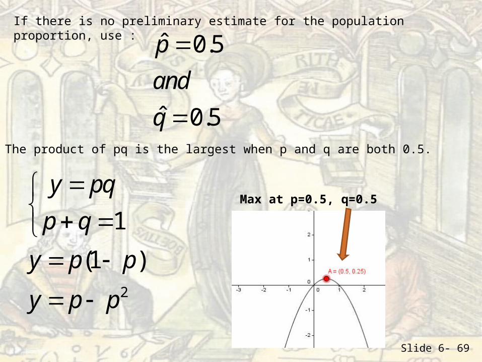
If there is no preliminary estimate for the population proportion, use :
ˆ 0.5
ˆ 0.5
p
and
q
The product of pq is the largest when p and q are both 0.5.
2
1
(1 )
y pq
p q
y p p
y p p
Max at p=0.5, q=0.5
Example: Sample Size
You are running a political campaign and wish to estimate, with 95% confidence, the proportion of registered voters who will vote for your candidate. Your estimate must be accurate within 3% of the true population. Find the minimum sample size needed if
1.no preliminary estimate is available.
Solution: Because you do not have a preliminary estimate for use and ˆ 5.0.q ˆ 0.5p p̂
70
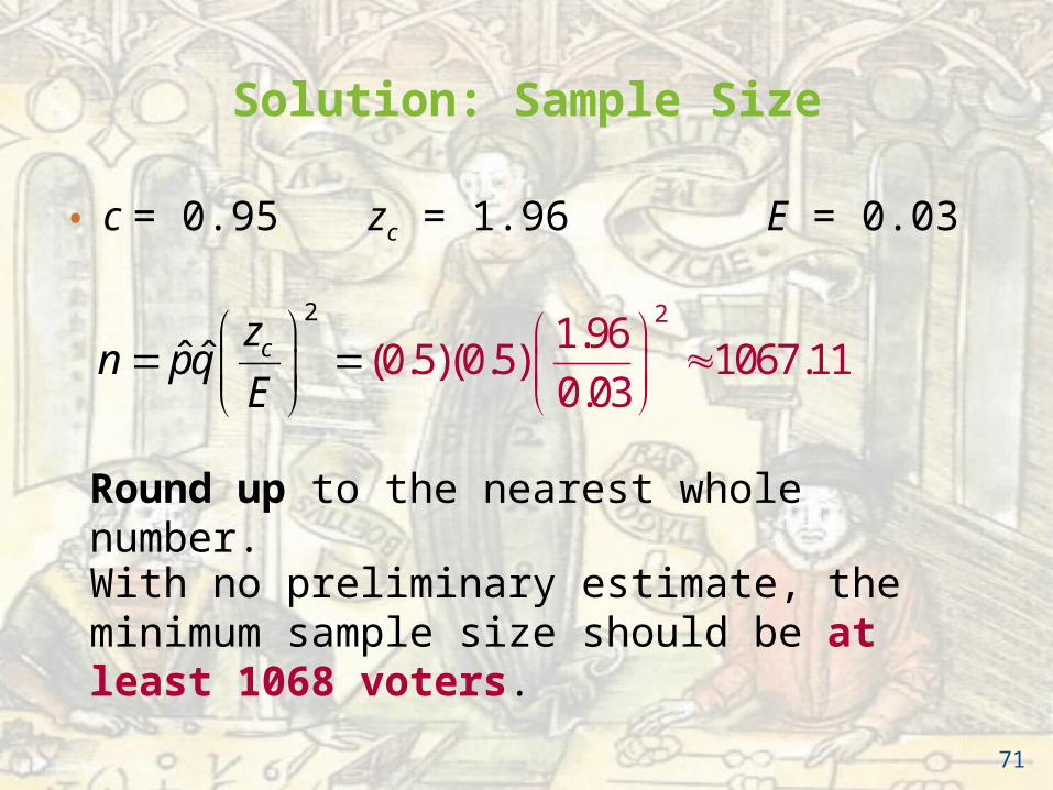
Solution: Sample Size
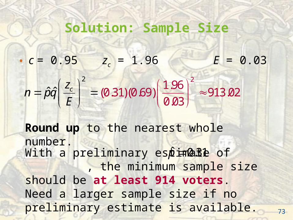
• c = 0.95 zc = 1.96 E = 0.03
2 21.96
(0.5)(0.5) 1067.110.
ˆ03
ˆ czn pq
E
Round up to the nearest whole number.
With no preliminary estimate, the minimum sample size should be at least 1068 voters.
71
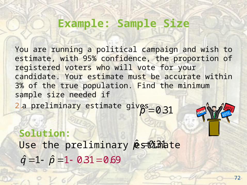
Example: Sample Size
You are running a political campaign and wish to estimate, with 95% confidence, the proportion of registered voters who will vote for your candidate. Your estimate must be accurate within 3% of the true population. Find the minimum sample size needed if
2.a preliminary estimate gives . ˆ 0.31p
Solution: Use the preliminary estimate
1 0.31 0. 9ˆ ˆ 61q p
ˆ 0.31p
72
Solution: Sample Size
• c = 0.95 zc = 1.96 E = 0.03
2 21.96
(0.31)(0.69) 913.020.
ˆ ˆ03
czn pq
E
Round up to the nearest whole number.
With a preliminary estimate of , the minimum sample size should be at least 914 voters.Need a larger sample size if no preliminary estimate is available.
ˆ 0.31p
73
Section 6.3 Summary
• Found a point estimate for the population proportion
• Constructed a confidence interval for a population proportion
• Determined the minimum sample size required when estimating a population proportion
74
Section 6.4
Confidence Intervals for Variance and Standard Deviation
75
Section 6.4 Objectives
• Interpret the chi-square distribution and use a chi-square distribution table
• Use the chi-square distribution to construct a confidence interval for the variance and standard deviation
76
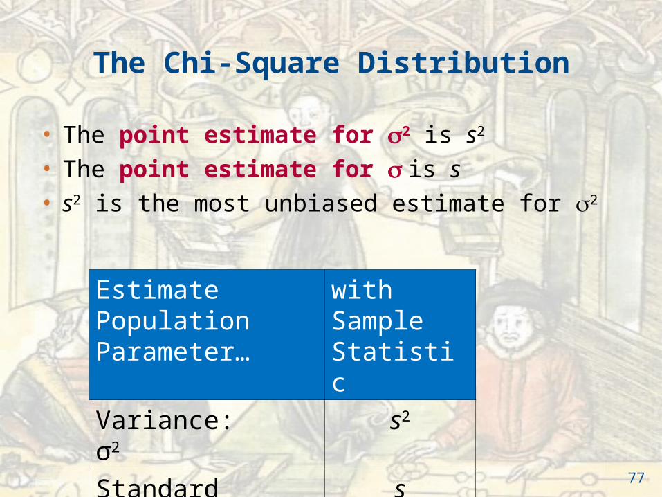
The Chi-Square Distribution
• The point estimate for 2 is s2
• The point estimate for is s
• s2 is the most unbiased estimate for 2
Estimate Population Parameter…
with Sample Statistic
Variance: σ2 s2
Standard deviation: σ s
77
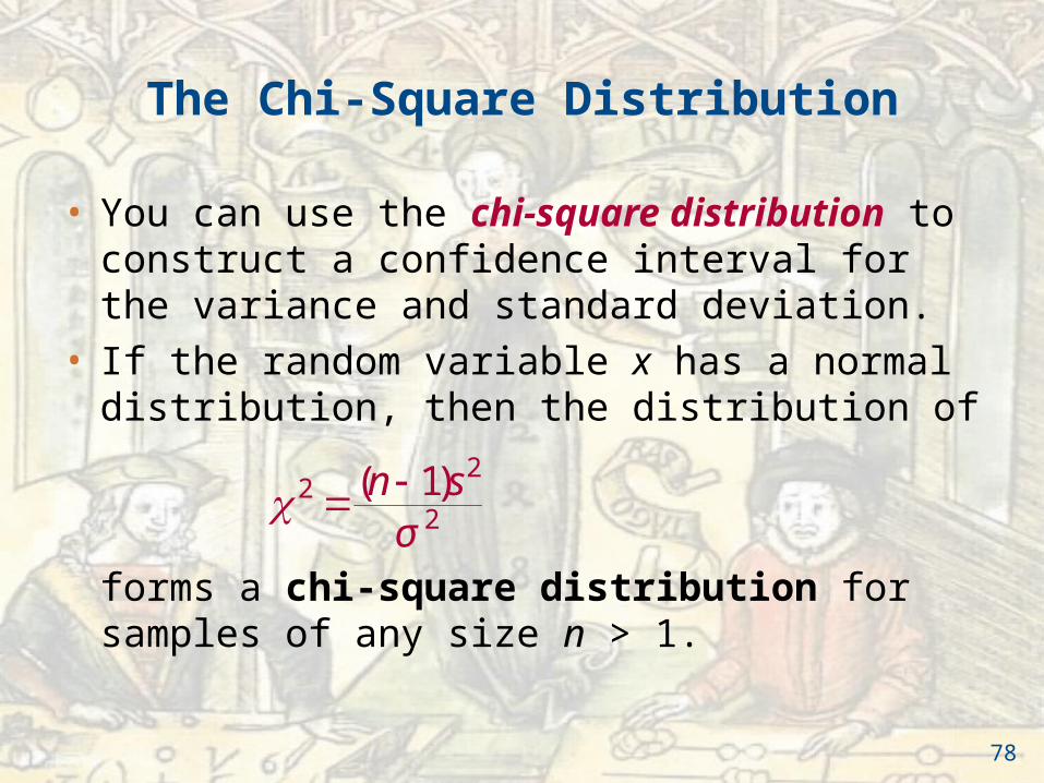
The Chi-Square Distribution
• You can use the chi-square distribution to construct a confidence interval for the variance and standard deviation.
• If the random variable x has a normal distribution, then the distribution of
forms a chi-square distribution for samples of any size n > 1.
22
2( 1)n s
σ
78
Slide 6- 79
The Chi-Square Distribution
Properties of The Chi-Square Distribution
1. All chi-square values χ2 are greater than or equal to zero.
2. The chi-square distribution is a family of curves, each determined by the degrees of freedom. To form a confidence interval for 2, use the χ2-distribution with degrees of freedom equal to one less than the sample size.
• d.f. = n – 1 Degrees of freedom
3. The area under each curve of the chi-square distribution equals one.
80
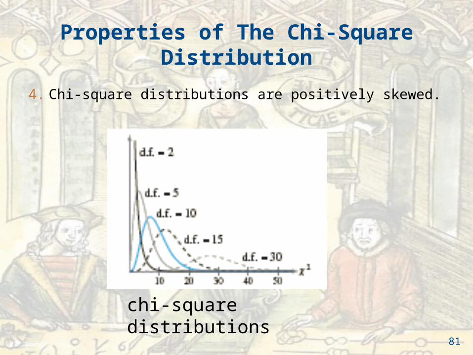
Properties of The Chi-Square Distribution
4. Chi-square distributions are positively skewed.
chi-square distributions
81
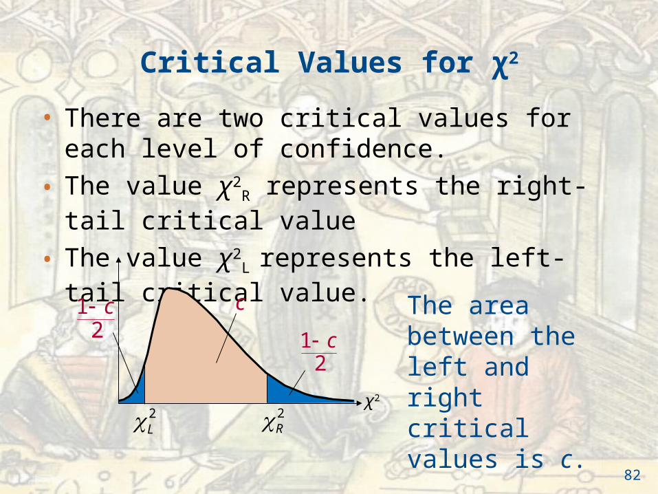
• There are two critical values for each level of confidence.
• The value χ2R represents the right-tail critical value
• The value χ2L represents the left-tail critical value.
Critical Values for χ2
The area between the left and right critical values is c.
χ2
c
12
c
12
c
2L 2
R
82
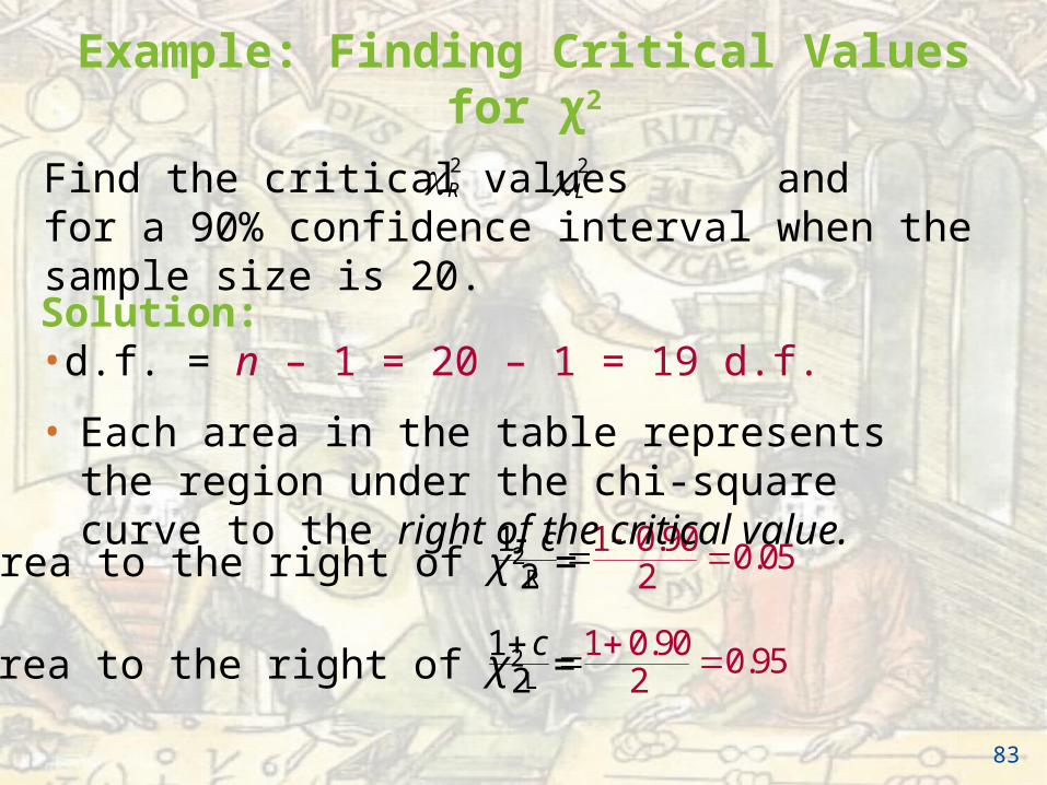
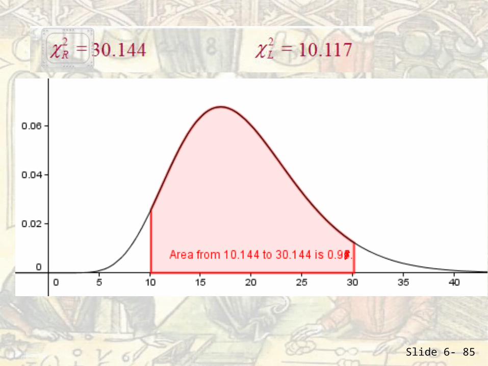
Example: Finding Critical Values for χ2
Find the critical values and for a 90% confidence interval when the sample size is 20.
Solution:•d.f. = n – 1 = 20 – 1 = 19 d.f.
• Area to the right of χ2R =
1 0.90 0.052
12
c
• Area to the right of χ2L =
1 0.90 0.952
12
c
2L2
R
83
• Each area in the table represents the region under the chi-square curve to the right of the critical value.
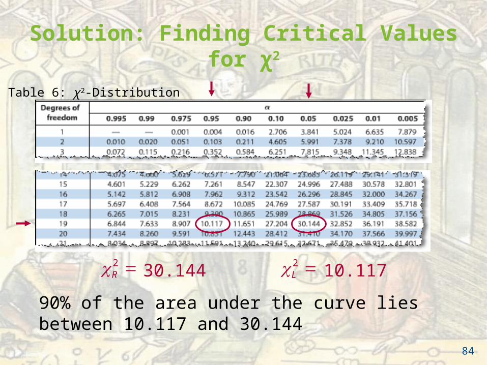
Solution: Finding Critical Values for χ2
Table 6: χ2-Distribution
2R 2
L
90% of the area under the curve lies between 10.117 and 30.144
84
30.144 10.117
Slide 6- 85
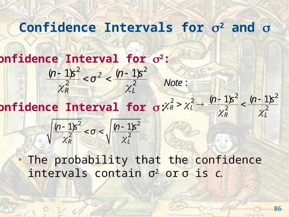
Confidence Interval for :
•
Confidence Intervals for 2 and
2 2
2 2( 1) ( 1)
R L
n s n s 2σ
• The probability that the confidence intervals contain σ2 or σ is c.
Confidence Interval for 2:
•
2 2
2 2( 1) ( 1)
R L
n s n s σ
86
2 22 2
2 2
:
( 1) ( 1)R L
R L
Note
n s n s
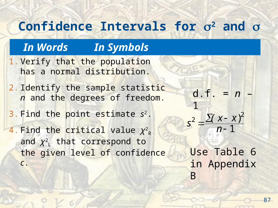
Confidence Intervals for 2 and
1. Verify that the population has a normal distribution.
2. Identify the sample statistic n and the degrees of freedom.
3. Find the point estimate s2.
4. Find the critical value χ2R and χ2
L that correspond to the given level of confidence c.
Use Table 6 in Appendix B
22 )
1x xsn
(
d.f. = n – 1
87
In Words In Symbols
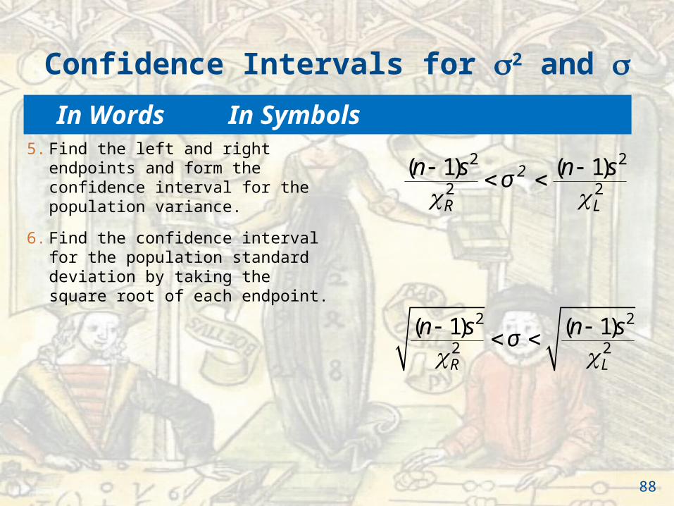
Confidence Intervals for 2 and
5. Find the left and right endpoints and form the confidence interval for the population variance.
6. Find the confidence interval for the population standard deviation by taking the square root of each endpoint.
2 2
2 2( 1) ( 1)
R L
n s n s 2σ
2 2
2 2( 1) ( 1)
R L
n s n s σ
88
In Words In Symbols
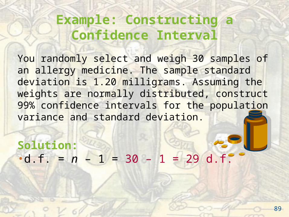
Example: Constructing a Confidence Interval
You randomly select and weigh 30 samples of an allergy medicine. The sample standard deviation is 1.20 milligrams. Assuming the weights are normally distributed, construct 99% confidence intervals for the population variance and standard deviation.
Solution:•d.f. = n – 1 = 30 – 1 = 29 d.f.
89
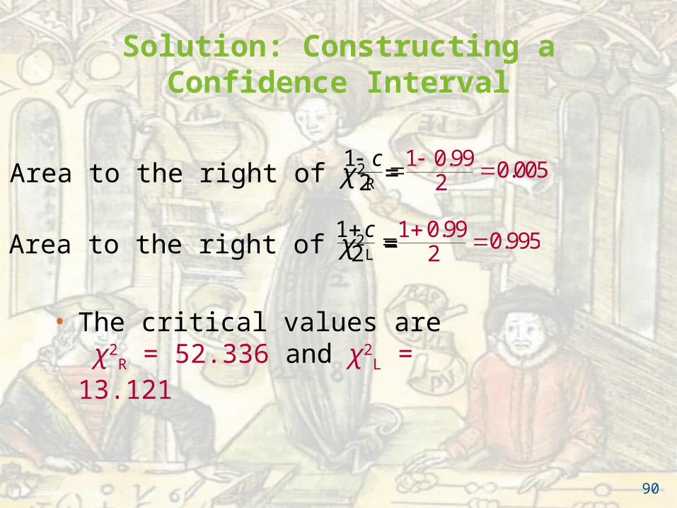
Solution: Constructing a Confidence Interval
• The critical values are χ2
R = 52.336 and χ2L = 13.121
• Area to the right of χ2R =
1 0.99 0.0052
12
c
• Area to the right of χ2L =
1 0.99 0.9952
12
c
90
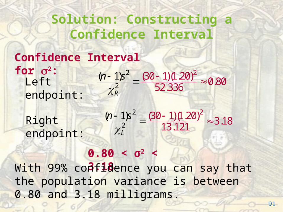
Solution: Constructing a Confidence Interval
2
22 (30 1)(1.20) 0.8052.336
( 1)
R
n s
Confidence Interval for 2:
2
22 (30 1)(1.20) 3.1813.121
( 1)
L
n s
Left endpoint:
Right endpoint:
0.80 < σ2 < 3.18With 99% confidence you can say that the population variance is between 0.80 and 3.18 milligrams.
91
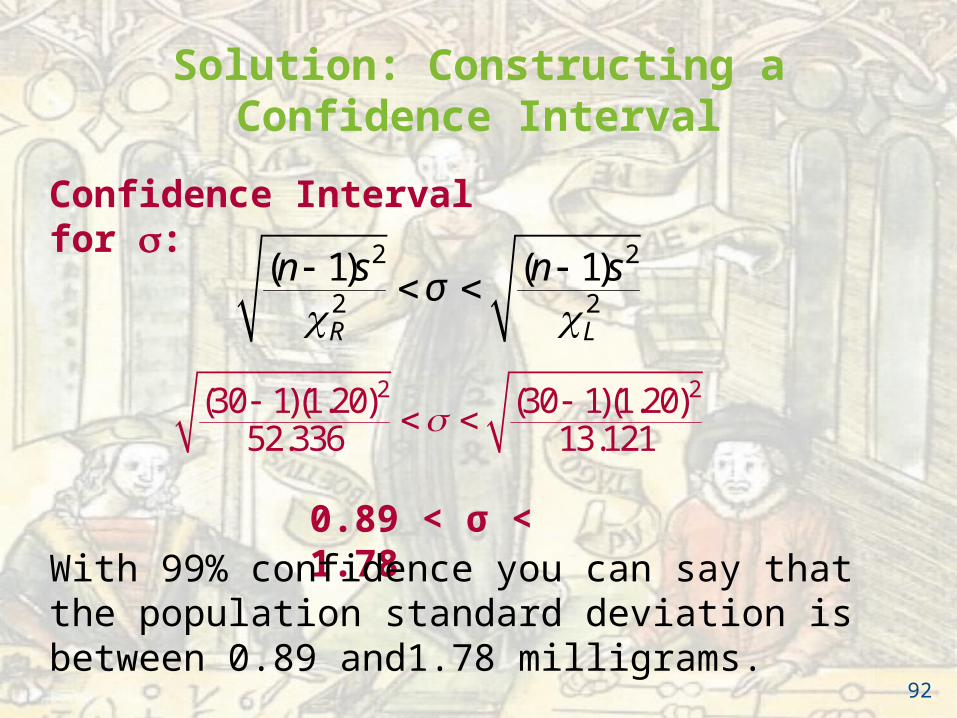
Solution: Constructing a Confidence Interval
2 2(30 1)(1.20) (30 1)(1.20)52.336 13.121
Confidence Interval for :
0.89 < σ < 1.78With 99% confidence you can say that the population standard deviation is between 0.89 and1.78 milligrams.
2 2
2 2( 1) ( 1)
R L
n s n s σ
92
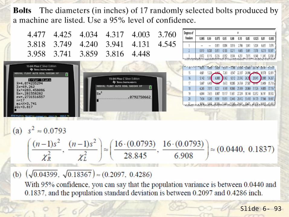
Slide 6- 93
Section 6.4 Summary
• Interpreted the chi-square distribution and used a chi-square distribution table
• Used the chi-square distribution to construct a confidence interval for the variance and standard deviation
94

Slide 6- 95
Control Charts
http://www.learner.org/courses/againstallodds/unitpages/unit23.html

Slide 4- 96
Elementary Statistics:
Picturing the World
Fifth Edition
by Larson and Farber
Chapter 6: Confidence Intervals
Slide 6- 97
A random sample of 42 textbooks has a mean price of $114.50 and a standard deviation of $12.30.
Find a point estimate for the mean price of all textbooks.
A. $42
B. $12.30
C. $114.50
D. $2.73
Slide 6- 98
A random sample of 42 textbooks has a mean price of $114.50 and a standard deviation of $12.30.
Find a point estimate for the mean price of all textbooks.
A. $42
B. $12.30
C. $114.50
D. $2.73
x
Slide 6- 99
Find the critical value zc necessary to form a 98% confidence interval.
A. 2.33
B. 2.05
C. 0.5040
D. 0.8365
Slide 6- 100
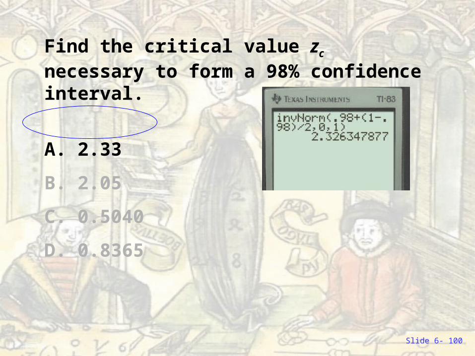
Find the critical value zc necessary to form a 98% confidence interval.
A. 2.33
B. 2.05
C. 0.5040
D. 0.8365
Slide 6- 101
A random sample of 42 textbooks has a mean price of $114.50 and a standard deviation of $12.30.
Find a 98% confidence interval for the mean price of all textbooks.
A. (111.38, 117.62)
B. (110.08, 118.92)
C. (110.78, 118.22)
D. (109.61, 119.39)
Slide 6- 102
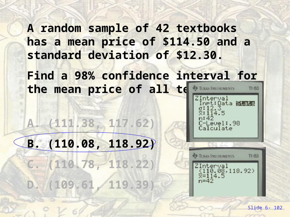
A random sample of 42 textbooks has a mean price of $114.50 and a standard deviation of $12.30.
Find a 98% confidence interval for the mean price of all textbooks.
A. (111.38, 117.62)
B. (110.08, 118.92)
C. (110.78, 118.22)
D. (109.61, 119.39)
Slide 6- 103
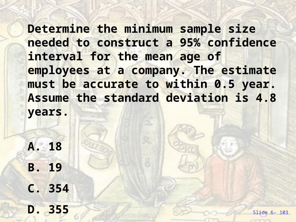
Determine the minimum sample size needed to construct a 95% confidence interval for the mean age of employees at a company. The estimate must be accurate to within 0.5 year. Assume the standard deviation is 4.8 years.
A. 18
B. 19
C. 354
D. 355
Slide 6- 104
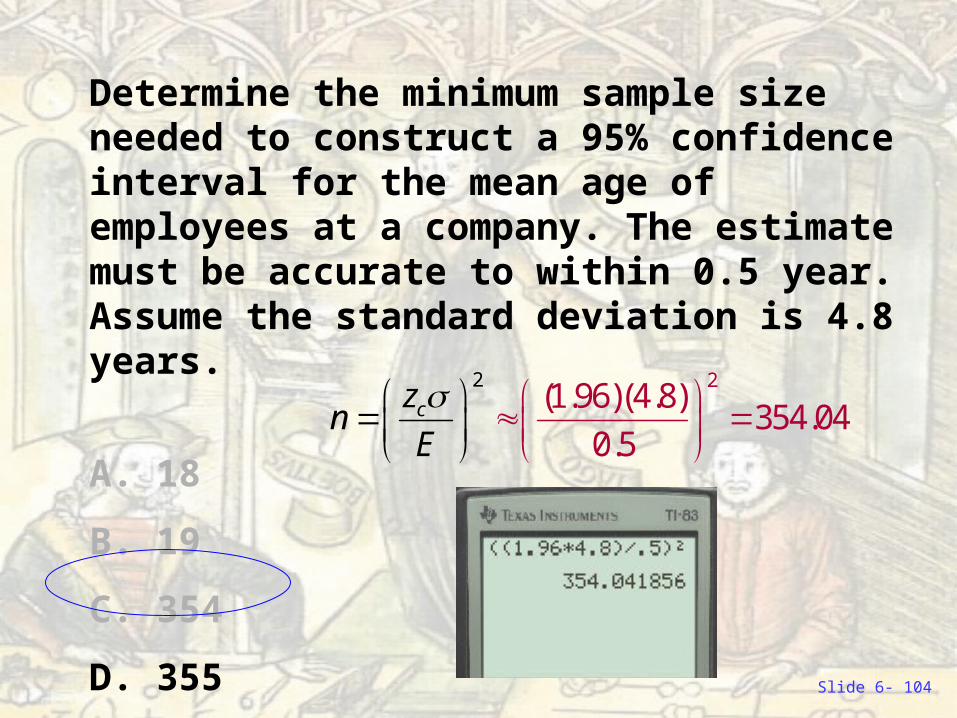
Determine the minimum sample size needed to construct a 95% confidence interval for the mean age of employees at a company. The estimate must be accurate to within 0.5 year. Assume the standard deviation is 4.8 years.
A. 18
B. 19
C. 354
D. 355
2 2(1.96)(4.8)
354.040.5
czn
E
Slide 6- 105
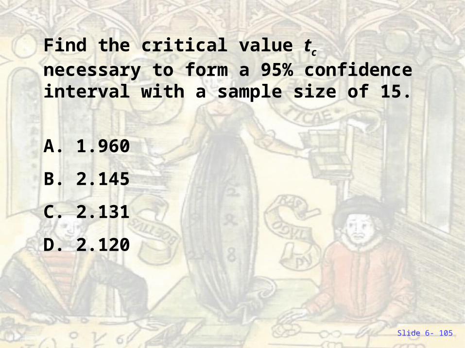
Find the critical value tc necessary to form a 95% confidence interval with a sample size of 15.
A. 1.960
B. 2.145
C. 2.131
D. 2.120
Slide 6- 106
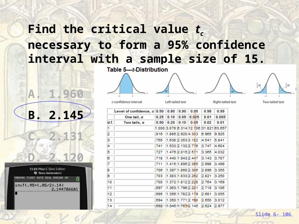
Find the critical value tc necessary to form a 95% confidence interval with a sample size of 15.
A. 1.960
B. 2.145
C. 2.131
D. 2.120
Slide 6- 107
A random sample of 15 DVD players has a mean price of $64.30 and a standard deviation of $5.60.
Find a 95% confidence interval for the mean price of all DVD players.
A. (61.20, 67.40)
B. (61.47, 67.13)
C. (61.22, 67.38)
D. (61.10, 67.51)
Slide 6- 108
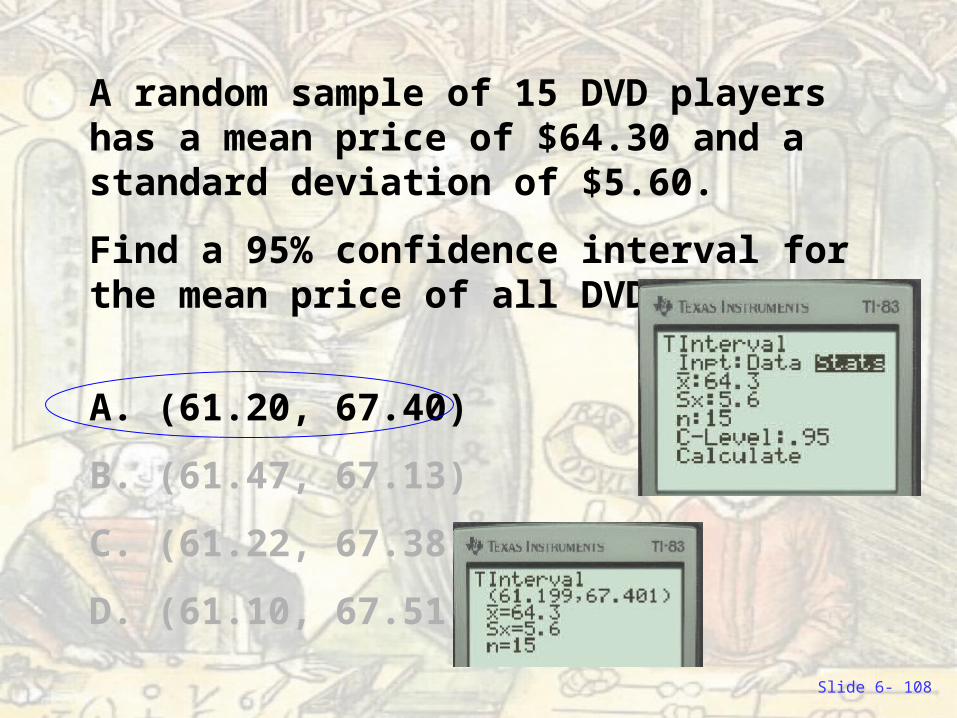
A random sample of 15 DVD players has a mean price of $64.30 and a standard deviation of $5.60.
Find a 95% confidence interval for the mean price of all DVD players.
A. (61.20, 67.40)
B. (61.47, 67.13)
C. (61.22, 67.38)
D. (61.10, 67.51)
Slide 6- 109
In a survey of 250 Internet users, 195 have high-speed Internet access at home.
Find a point estimate for the proportion of all Internet users who have high-speed Internet access at home.
A. 1.28
B. 0.78
C. 0.22
D. 195
Slide 6- 110
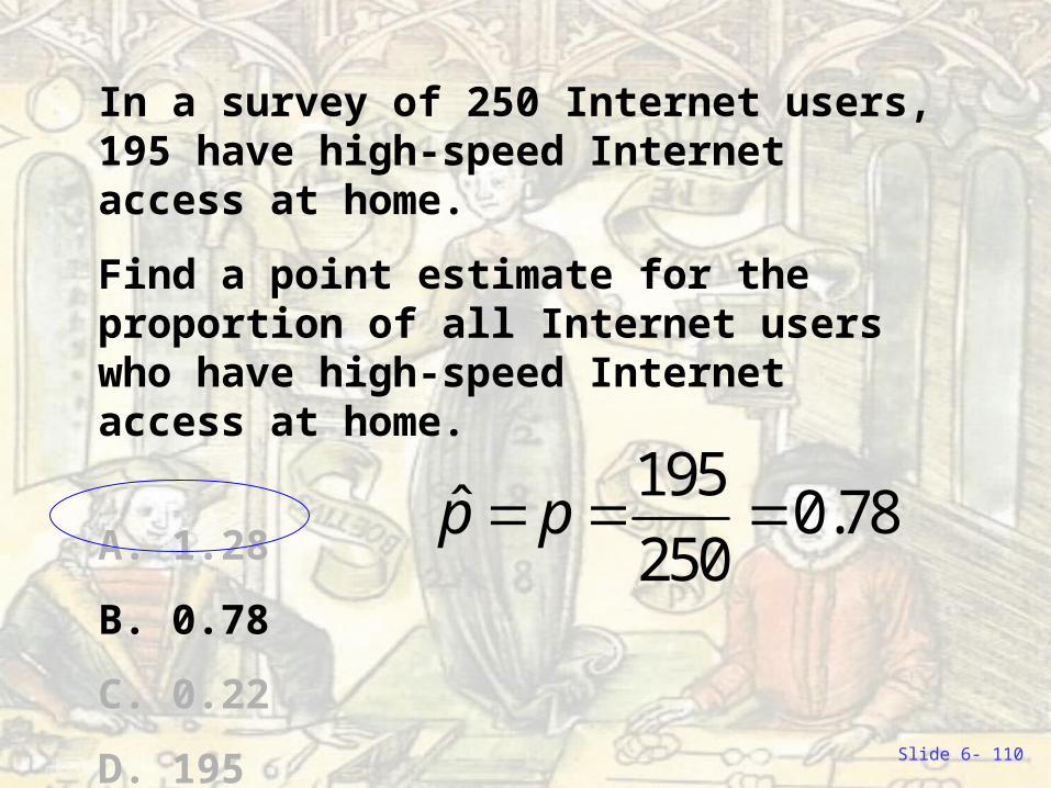
In a survey of 250 Internet users, 195 have high-speed Internet access at home.
Find a point estimate for the proportion of all Internet users who have high-speed Internet access at home.
A. 1.28
B. 0.78
C. 0.22
D. 195
195ˆ 0.78
250p p
Slide 6- 111
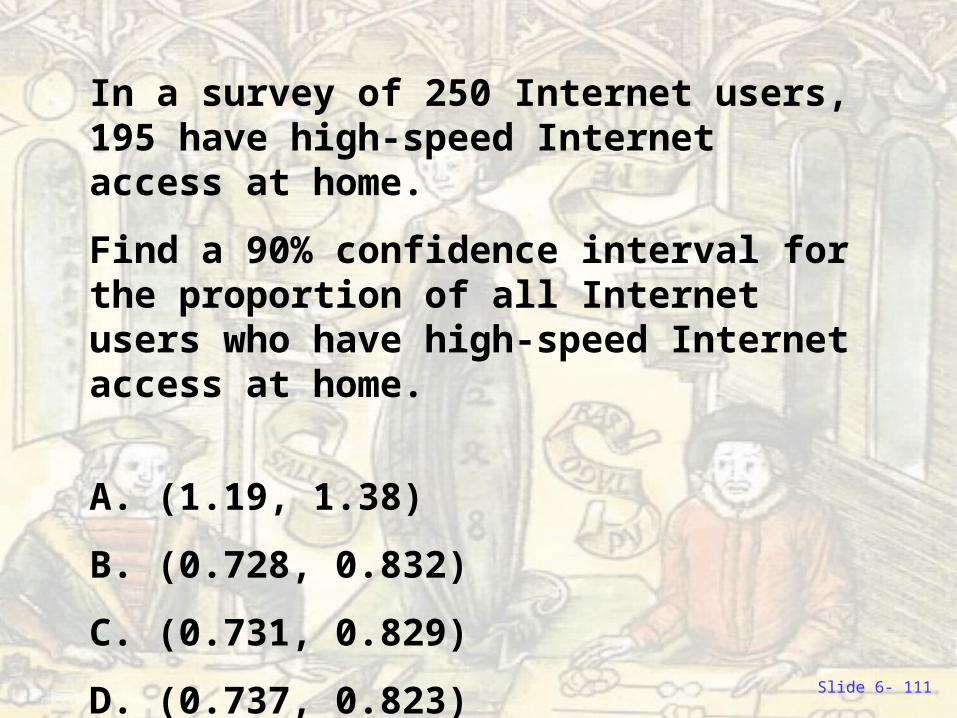
In a survey of 250 Internet users, 195 have high-speed Internet access at home.
Find a 90% confidence interval for the proportion of all Internet users who have high-speed Internet access at home.
A. (1.19, 1.38)
B. (0.728, 0.832)
C. (0.731, 0.829)
D. (0.737, 0.823)
Slide 6- 112
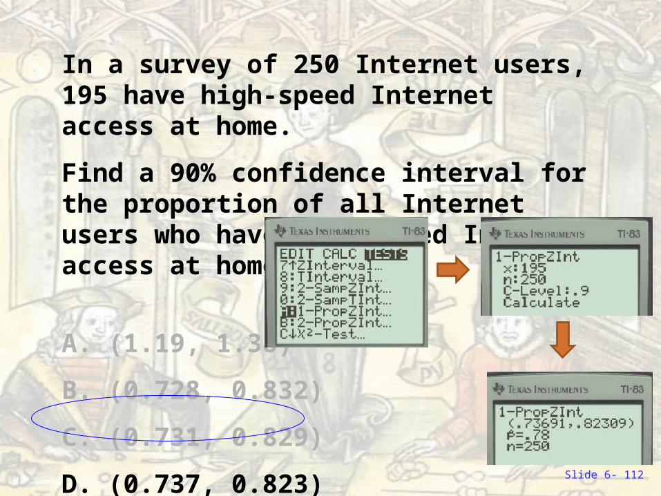
In a survey of 250 Internet users, 195 have high-speed Internet access at home.
Find a 90% confidence interval for the proportion of all Internet users who have high-speed Internet access at home.
A. (1.19, 1.38)
B. (0.728, 0.832)
C. (0.731, 0.829)
D. (0.737, 0.823)
Slide 6- 113
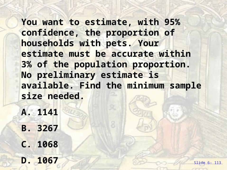
You want to estimate, with 95% confidence, the proportion of households with pets. Your estimate must be accurate within 3% of the population proportion. No preliminary estimate is available. Find the minimum sample size needed.
A. 1141
B. 3267
C. 1068
D. 1067
Slide 6- 114
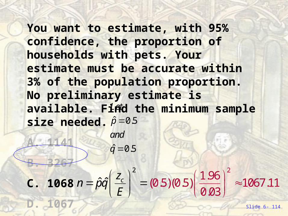
You want to estimate, with 95% confidence, the proportion of households with pets. Your estimate must be accurate within 3% of the population proportion. No preliminary estimate is available. Find the minimum sample size needed.
A. 1141
B. 3267
C. 1068
D. 10672 2
1.96(0.5)(0.5) 1067.11
0.ˆ
03ˆ cz
n pqE
ˆ 0.5
ˆ 0.5
Let
p
and
q
Slide 6- 115
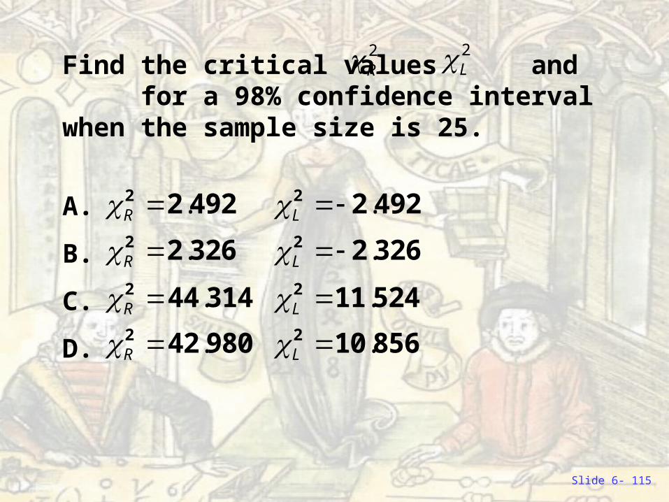
Find the critical values and for a 98% confidence interval when the sample size is 25.
A.
B.
C.
D.
2R 2
L
.R 2 42 980 .L 2 10 856
.R 2 44 314 .L 2 11 524
.R 2 2 326 .L 2 2 326
.R 2 2 492 .L 2 2 492
Slide 6- 116
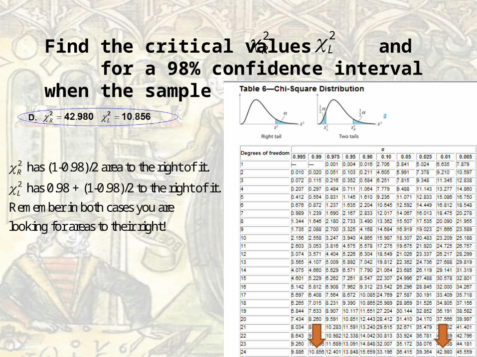
Find the critical values and for a 98% confidence interval when the sample size is 25.
2R 2
L
2
2
has (1-0.98)/2 area to the right of it.
has 0.98 + (1-0.98)/2 to the right of it.
Remember in both cases you are
looking for areas to their right!
R
L