Page 1 of 61

Introduction to Modal Intervals

Prepared for the IEEE 1788 Working Group

by

Nathan T. Hayes1, Sunfish Studio, LLC

August 21, 2009

This paper is intended to provide an introductory tour of the modal intervals. It is

geared for people who already have a set-theoretic background and are interested

to learn about the modal interval perspective. The purpose is to present a practical

introduction to a subject that otherwise seems to have received little attention over

the years, perhaps because it has a reputation of being difficult to understand. This

paper also presents some new and recent work of Sunfish, so it captures our

perspective on modal intervals as it relates to interval standardization. For all these

reasons, only the most relevant details are presented. The interested reader can find

a wealth of deeper discussion in the references.

1 Background

The common and popular notion of interval arithmetic is based on the fundamental

premise that intervals are sets of numbers and that arithmetic operations can be

performed on these sets. This interpretation of interval arithmetic, popularized by

Ramon E. Moore, has received a great deal of attention and development by interval

researchers. It is sometimes referred to as the “classical” interval arithmetic, and it

is purely set-theoretic in nature.

Modal intervals, conceived by E. Gardenes in 1985 and studied earlier in various

forms by mathematicians such as M. Warmus (1956), T. Sunaga (1958), H. J. Ortolf

(1969), E. Kaucher (1973) and N. Dimitrova, S. Markov and E. Popova (1992), can

be thought of as an extension of the classical intervals. Before starting a discussion

of modal intervals, though, many people often want to know “why?” In other words,

what is the need for the modal intervals? Why aren’t the set-theoretic intervals

“good enough?” What kind of “extensions” do the modal intervals really provide?

These are good questions, and this paper will try to answer them in a simple and

straightforward manner. One way to see a motivation for the modal intervals is to

take a closer look at some of the shortcomings of a purely set-theoretic approach. So

this is where the paper begins. 1 Special thanks to G. W. Walster, E. Hansen, A. Neumaier and S. Markov for helpful and productive discussions, as well as M. A. Sainz and E. Popova for reviewing this paper. Positions presented are my own and not necessarily those of these persons.

Page 2 of 61

1.1 Classical Intervals

The set of real numbers 𝐑 is uncountable, therefore a computer must perform

calculations upon a finite subset of 𝐑. A digital scale is such a subset. Each mark in a

digital scale is represented in a computer by a bit-pattern and corresponds to a

particular element of 𝐑 (the same applies if 𝐑∗, the set of extended-reals, is

considered, but for the sake of simplicity this paper only considers 𝐑).

For all that computationally matters, the real operators are introduced into the

system of set-theoretic intervals

𝐼 𝐑 ∶= 𝑎, 𝑏 𝑎 ∈ 𝐑, 𝑏 ∈ 𝐑,𝑎 ≤ 𝑏

by defining interval operators for addition, subtraction, multiplication and division

such that any two interval operands produce an interval result which contains every

arithmetical combination of numbers belonging to the operands. If computing on a

digital scale, interval operators employ an outer rounding to guarantee containment

of the interval operands in the interval result.

The interval functions 𝑓𝑅 of system 𝐼 𝐑 are then defined by replacing the real

operators of the real functions by the respective interval operators. By means of this

process the guarantee promised by the fundamental theorem of interval arithmetic

is obtained, i.e., all solutions are contained in the interval result. This forms the basis

of a large body of work made famous by classical interval analysis. For this reason, it

won’t be reiterated here in any further detail.

1.2 Amplification of Dependence

For any number of set-theoretic interval operands 𝑋1,… ,𝑋𝑛 ∈ 𝐼 𝐑 , the amount of

pessimism, even when exact arithmetic on 𝐑 is used, between the set of values of a

real function

𝑓 𝑥1,… , 𝑥𝑛 𝑥1,… , 𝑥𝑛 ∈ 𝑋1,… ,𝑋𝑛

and the enclosure of its interval computation 𝑓𝑅(𝑋1,… ,𝑋𝑛) is often greater than a

reasonable expected approximation when some argument variables 𝑥1,… , 𝑥𝑛 appear

multiple times in the expression of the real function 𝑓(… ), i.e., when some

components of argument 𝑥 = (𝑥1,… , 𝑥𝑛) are multi-incident in the syntax tree of the

function 𝑓(… ).

As an example, it is enough to compare, for 𝑥 ∈ 𝑋 = [1,2], the set of values of the

real function 𝑓 𝑥 ≔ 𝑥 − 𝑥, which is 𝑥 − 𝑥 𝑥 ∈ 1,2 = [0,0], with the result of

the interval operation on 𝐼 𝐑 ,

𝑓𝑅 𝑋 ∶= 𝑋 − 𝑋 = 1,2 − 1,2 ∶= 𝑥 − 𝑦 𝑥 ∈ 1,2 ,𝑦 ∈ 1,2 = [−1,1].

This phenomenon is called “amplification of dependence.” It is a well-known and

Page 3 of 61

familiar difficulty with interval computations, as it often leads to overly pessimistic

results.

1.3 Sub-distributive Law

In the system 𝐼 𝐑 , the distributive property of multiplication is weakened with

regard to addition and becomes a sub-distributive law, i.e.,

𝐴 ⋅ 𝐵 + 𝐶 ⊆ 𝐴 ⋅ 𝐵 + 𝐴 ⋅ 𝐶.

As an example, consider

1,3 ⋅ 1,1 + −1,−1 = 0,0 ⊆ 1,3 ⋅ 1,1 + 1,3 ⋅ −1,−1 = [−2,2].

The unwanted consequence of a sub-distributive law is increased pessimism similar

to the amplification of dependence. However, the dependence in this case is due

specifically to the weakened distributive properties of multiplication over addition

in the system 𝐼 𝐑 .

1.4 Empty Set

In mathematics, a lattice is a partially ordered set for which the subsets of any two

elements have a unique infimum and supremum. The real numbers ordered by the

less-or-equal relation ≤ forms a lattice, and the breaking points ( 𝑥 ≤ 𝑦 | 𝑥 ≥ 𝑦 ) for

any 𝑥,𝑦 ∈ 𝐑 is binary. For example, 𝑥 and 𝑦 have two possible situations relative to

each other, i.e., either 𝑥 ≤ 𝑦 or 𝑥 ≥ 𝑦. By comparison, the lattice on 𝐼 𝐑 has four

breaking points according to

𝑋 ⊆ 𝑌 𝑋 ⊇ 𝑌 𝑋 ≤ 𝑌 𝑋 ≥ 𝑌 )

for any 𝑋,𝑌 ∈ 𝐼 𝐑 . The system of comparison relations (𝐼 𝐑 ,≤,≥) is the partial

order complementary to the partial order (𝐼 𝐑 ,⊆,⊇).

Intersection, i.e., the system (𝐼 𝐑 ,∩), is not closed with respect to the inclusion

relations (𝐼 𝐑 ,⊆,⊇). If classical intervals 𝐴 and 𝐵 are disjoint, the operation 𝐴 ∩ 𝐵

produces the empty set, which is not an element of 𝐼 𝐑 .

It is remarkable how, in classical analysis, the empty set is taken for granted. In

some cases it is used constructively, as in proving the non-existence of zeros in the

interval Newton method. In other cases it can add a great deal of special handling to

algorithms and interval libraries. Modal intervals, however, reveal that the empty

set is an unnecessary consequence of an incomplete interval structure. It is also an

obstacle to important numerical capabilities, such as computing the inner rounding

or enclosure of an expression. Even without an empty set, the modal intervals are

capable of providing proofs of non-existence, as in the case of the interval Newton

method. More on this topic will be discussed later.

Page 4 of 61

2 Logic

Unlike classical intervals, the set-membership reasoning of modal intervals is based

entirely on predicate logic. For this reason, modal intervals are grounded not only in

set-theory but also in the theory of propositions and logic.

While it is a broad subject and runs very deep in the literature on modal intervals,

the purpose of this paper is to introduce and illustrate the basic concepts. For this

reason, some boilerplate material is quickly reviewed.

2.1 Propositions

A proposition is a statement that is either true or false, but not both. Propositional

logic, in general, lends itself well to digital computing because computers operate in

terms of binary representations, e.g., “true” or “false,” “on” or “off,” etc.

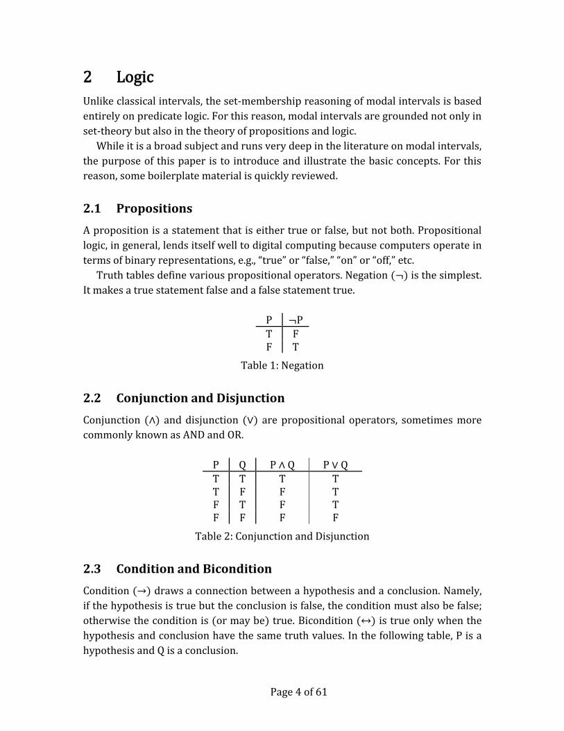
Truth tables define various propositional operators. Negation (¬) is the simplest.

It makes a true statement false and a false statement true.

P ¬P

T F F T

Table 1: Negation

2.2 Conjunction and Disjunction

Conjunction ∧ and disjunction ∨ are propositional operators, sometimes more

commonly known as AND and OR.

P Q P ∧ Q P ∨ Q

T T T T T F F T F T F T F F F F

Table 2: Conjunction and Disjunction

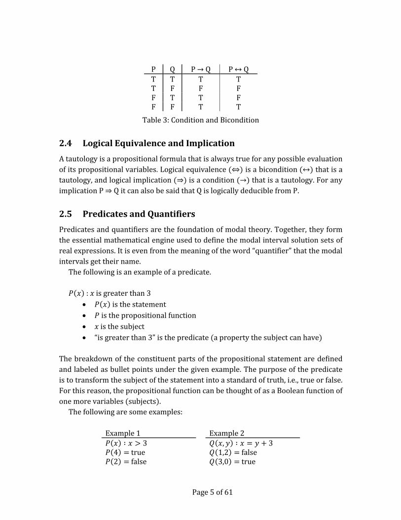
2.3 Condition and Bicondition

Condition → draws a connection between a hypothesis and a conclusion. Namely,

if the hypothesis is true but the conclusion is false, the condition must also be false;

otherwise the condition is (or may be) true. Bicondition ↔ is true only when the

hypothesis and conclusion have the same truth values. In the following table, P is a

hypothesis and Q is a conclusion.

Page 5 of 61

P Q P → Q P ↔ Q

T T T T T F F F F T T F F F T T

Table 3: Condition and Bicondition

2.4 Logical Equivalence and Implication

A tautology is a propositional formula that is always true for any possible evaluation

of its propositional variables. Logical equivalence ⇔ is a bicondition ↔ that is a

tautology, and logical implication ⇒ is a condition → that is a tautology. For any

implication P ⇒ Q it can also be said that Q is logically deducible from P.

2.5 Predicates and Quantifiers

Predicates and quantifiers are the foundation of modal theory. Together, they form

the essential mathematical engine used to define the modal interval solution sets of

real expressions. It is even from the meaning of the word “quantifier” that the modal

intervals get their name.

The following is an example of a predicate.

𝑃 𝑥 : 𝑥 is greater than 3

𝑃 𝑥 is the statement

𝑃 is the propositional function

𝑥 is the subject

“is greater than 3” is the predicate a property the subject can have)

The breakdown of the constituent parts of the propositional statement are defined

and labeled as bullet points under the given example. The purpose of the predicate

is to transform the subject of the statement into a standard of truth, i.e., true or false.

For this reason, the propositional function can be thought of as a Boolean function of

one more variables (subjects).

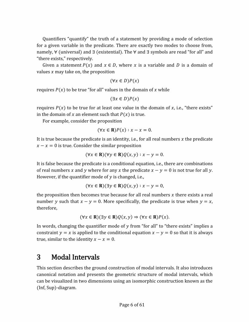
The following are some examples:

Example 1 Example 2

𝑃 𝑥 ∶ 𝑥 > 3 𝑃 4 = true 𝑃 2 = false

𝑄 𝑥,𝑦 ∶ 𝑥 = 𝑦 + 3 𝑄 1,2 = false 𝑄 3,0 = true

Page 6 of 61

Quantifiers “quantify” the truth of a statement by providing a mode of selection

for a given variable in the predicate. There are exactly two modes to choose from,

namely, ∀ universal and ∃ existential). The ∀ and ∃ symbols are read “for all” and

“there exists,” respectively.

Given a statement 𝑃(𝑥) and 𝑥 ∈ 𝐷, where 𝑥 is a variable and 𝐷 is a domain of

values 𝑥 may take on, the proposition

(∀𝑥 ∈ 𝐷)𝑃(𝑥)

requires 𝑃(𝑥) to be true “for all” values in the domain of 𝑥 while

(∃𝑥 ∈ 𝐷)𝑃(𝑥)

requires 𝑃(𝑥) to be true for at least one value in the domain of 𝑥, i.e., “there exists”

in the domain of 𝑥 an element such that 𝑃(𝑥) is true.

For example, consider the proposition

(∀𝑥 ∈ 𝐑)𝑃 𝑥 ∶ 𝑥 − 𝑥 = 0.

It is true because the predicate is an identity, i.e., for all real numbers 𝑥 the predicate

𝑥 − 𝑥 = 0 is true. Consider the similar proposition

(∀𝑥 ∈ 𝐑)(∀𝑦 ∈ 𝐑)𝑄 𝑥,𝑦 ∶ 𝑥 − 𝑦 = 0.

It is false because the predicate is a conditional equation, i.e., there are combinations

of real numbers 𝑥 and 𝑦 where for any 𝑥 the predicate 𝑥 − 𝑦 = 0 is not true for all 𝑦.

However, if the quantifier mode of 𝑦 is changed, i.e.,

(∀𝑥 ∈ 𝐑)(∃𝑦 ∈ 𝐑)𝑄 𝑥,𝑦 ∶ 𝑥 − 𝑦 = 0,

the proposition then becomes true because for all real numbers 𝑥 there exists a real

number 𝑦 such that 𝑥 − 𝑦 = 0. More specifically, the predicate is true when 𝑦 = 𝑥,

therefore,

(∀𝑥 ∈ 𝐑)(∃𝑦 ∈ 𝐑)𝑄 𝑥,𝑦 ⇒ (∀𝑥 ∈ 𝐑)𝑃 𝑥 .

In words, changing the quantifier mode of 𝑦 from “for all” to “there exists” implies a

constraint 𝑦 = 𝑥 is applied to the conditional equation 𝑥 − 𝑦 = 0 so that it is always

true, similar to the identity 𝑥 − 𝑥 = 0.

3 Modal Intervals

This section describes the ground construction of modal intervals. It also introduces

canonical notation and presents the geometric structure of modal intervals, which

can be visualized in two dimensions using an isomorphic construction known as the

(Inf, Sup)-diagram.

Page 7 of 61

3.1 Ground Construction of Modal Intervals

The ground construction of modal intervals is provided by

The set of real numbers 𝐑

The set of set-theoretic intervals 𝐼 𝐑

The set of classic predicates on the real line, 𝑃 . ∶ 𝐑 → true, false .

More particularly, if

Pred(𝐑) ∶= 𝑃(. ) 𝑃 . ∶ 𝐑 → true, false

is the set of classic predicates on the real line and

Pred(𝑥) ∶= 𝑃(. ) ∈ Pred(𝐑) 𝑃 𝑥 = true

is the set of predicates a real number 𝑥 accepts, then modal analysis stands on the

identification

𝑥 ⟷ Pred(𝑥).

This is the main point of departure from the classical analysis which instead builds

on a singleton interpretation of real numbers 𝑥 ⟷ 𝑥 .

A modal interval 𝑋 is an element of the cartesian product (𝑋′,𝑄) where 𝑋′ ∈ 𝐼 𝐑

is a set-theoretic interval and 𝑄 ∈ ∃,∀ is one of the classic quantifier modes. In

the modal interval literature, it is traditional to delimit set-theoretic intervals with

an apostrophe to distinguish them from modal intervals. The remainder of this

paper follows this convention.

From this perspective, it is common to think of the modal intervals

𝐼∗ 𝐑 ∶= 𝑋′,𝑄 𝑋′ ∈ 𝐼 𝐑 , 𝑄 ∈ ∀,∃

as quantified set-theoretic intervals. This is a similar method to that in which real

numbers are associated in pairs having the same absolute value but opposite signs.

Modal intervals in the system 𝐼∗ 𝐑 are likewise associated in pairs having the same

set but opposite modes.

For any modal interval, the quantifier “for all” or “there exists” describes how the

set-theoretic component must be used in a propositional statement. For example, if

𝐴 = 1,2 ′,∀ and 𝐵 = 1,2 ′,∃ are universal and existential modal intervals, and if

𝑃(𝑥) is a real predicate, then the proposition

∀𝑎 ∈ 𝐴′ 𝑃(𝑎)

requires the predicate 𝑃(𝑎) to be true for all 𝑎 ∈ [1,2]′ and the proposition

∃𝑏 ∈ 𝐵′ 𝑃(𝑏)

requires the predicate 𝑃(𝑏) to be true only for at least one 𝑏 ∈ [1,2]′.

Page 8 of 61

These concepts connect intuitively to the fact that in computational operations on

digital numerical information, an interval result 𝑋′ points to, and bounds, some real

number 𝑥 (or set of numbers) holding a determinate property 𝑃(𝑥). For example, an

interval may specify a tolerable limit of some unknown value, like a measurement.

In this case, it is important that a reliable solution must consider all of the possible

elements within the interval. But an interval may also specify a predetermined error

bound from which elements must be drawn or selected “a posteriori” in order to

regulate a system or solve an equation. In both examples the interval is interpreted

in one of two different ways: the former according to a universal and the latter to an

existential mode.

This idea is generalized even further by considering the set of real predicates

accepted by a modal interval, i.e.,

Pred((𝑋′,𝑄)) ∶= 𝑃(. ) ∈ Pred(𝐑) 𝑄𝑥 ∈ 𝑋′ 𝑃 𝑥 = true .

By this definition it is possible to consider the entire family of propositions

𝑄𝑥 ∈ 𝑋′ 𝑃 𝑥

which a modal interval (𝑋′,𝑄) validates.

3.2 Canonical Notation and Coordinates

For 𝑎, 𝑏 ∈ 𝐑, the canonical notation of a modal interval is

𝑎, 𝑏 ∶= 𝑎, 𝑏 ′,∃ 𝑖𝑓 𝑎 ≤ 𝑏

𝑏,𝑎 ′,∀ 𝑖𝑓 𝑎 ≥ 𝑏

With canonical notation, it is possible to express the set 𝐼∗ 𝐑 of modal intervals

in “natural” terms, i.e.,

𝐼∗ 𝐑 ∶= 𝑎, 𝑏 𝑎 ∈ 𝐑, 𝑏 ∈ 𝐑 .

This reveals another reason why modal intervals are an extension of the classical

intervals. In words, 𝐼 𝐑 is isomorphic to a portion of 𝐼∗ 𝐑 , namely the existential

modal intervals.

Canonical notation is a convenient notational scheme. Many practical theorems,

formulas and implementation strategies take advantage of canonical notation. In all

cases, the true mathematical properties of a modal interval can be deduced from the

canonical notation.

Coordinates describe the intrinsic properties of a modal interval. Because this is

an introductory paper, definitions are given without justification. For a canonical

modal interval 𝑋 = [𝑎, 𝑏], the coordinates are

Inf(𝑋) ∶= 𝑎 Sup(𝑋) ∶= 𝑏 Mode(𝑋) ∶= ∃ 𝑖𝑓 𝑎 ≤ 𝑏∀ 𝑖𝑓 𝑎 ≥ 𝑏

Page 9 of 61

and the set-theoretical component is obtained by

Set 𝑋 ∶= [min 𝑎, 𝑏 , max 𝑎, 𝑏 ]′.

For example, if [5,9] and [3,2] are canonical modal intervals, then

Inf Sup Mode Set

[5,9] 5 9 ∃ [5,9]′ [3,2] 3 2 ∀ [2,3]′

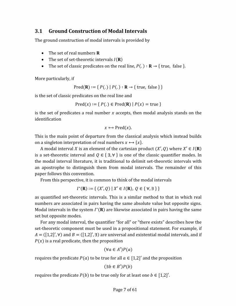
Canonical notation and coordinates provide a useful geometric interpretation of

the modal intervals. This interpretation, called the (Inf, Sup)-diagram, is depicted in

Figure 1. Every modal interval 𝑋 ∈ 𝐼∗ 𝐑 appears in the diagram as a point with the

coordinates (Inf(𝑋), Sup(𝑋)). The diagram is isomorphic to 𝐼∗ 𝐑 , and it is useful

because it reveals the underlying structure of the modal intervals. The Inf = Sup line

is the set of all real numbers, i.e., the set of degenerate modal intervals. The half

plane above is the set of existential intervals, and the half plane below is the set of

universal modal intervals. For degenerate modal intervals, quantifier modes “for all”

and “there exists” coincide, i.e., they have the same meaning.

The (Inf, Sup)-diagram reveals the structural difference between the classical and

modal intervals. For example, the shaded area below the Inf = Sup line represents a

Figure 1: (Inf, Sup)-diagram

Sup

Inf

A (existential)

B (universal)

C (point)

R (the real numbers)

Page 10 of 61

set of invalid intervals that do not belong to the 𝐼 𝐑 system. But this is the set of

universal modal intervals in the 𝐼∗ 𝐑 system. If one views the (Inf, Sup)-diagram as

an interval analogy of 𝐑 divided into complementary sets of positive and negative

real numbers, a geometric insight is then provided into why 𝐼 𝐑 is not structurally

complete. Restricting interval arithmetic to 𝐼 𝐑 is, by analogy, like restricting real

arithmetic on 𝐑 to the non-negative real numbers. Only the system 𝐼∗ 𝐑 completes

the analogy by providing complementary sets of intervals, i.e., the existential and

universal modal intervals.

4 Relations and Lattice Operators

The modal interval comparison relations on 𝐼∗ 𝐑 are mostly analogous to their set-

theoretic counterparts on 𝐼 𝐑 . However there is also a surprising difference. This

section of the paper presents an overview of this important distinction.

4.1 Comparison Relations

For any 𝐴,𝐵 ∈ 𝐼∗ 𝐑 , the identification of modal intervals with the sets of predicates

they accept is consistently used by the definition of modal inclusion

𝐴 ⊆ 𝐵 ∶= Pred(𝐴) ⊆ Pred(𝐵).

This leads to the implication

Pred(𝐴) ⇒ Pred(𝐵),

and the set-theoretic projection of modal inclusion is subsequently established. The

following table is a summary of the results:

Mode(𝐴) Mode(𝐵) Relation Projection ∃ ∃ 𝐴 ⊆ 𝐵 ⇔ Set(𝐴) ⊆ Set(𝐵) ∀ ∀ 𝐴 ⊆ 𝐵 ⇔ Set(𝐴) ⊇ Set(𝐵) ∀ ∃ 𝐴 ⊆ 𝐵 ⇔ Set(𝐴) ∩ Set(𝐵) ≠ ∅ ∃ ∀ 𝐴 ⊆ 𝐵 ⇔ Inf 𝐴 = Sup 𝐴 = Inf 𝐵 = Sup 𝐵

Modal intervals may also be associated with the set of real predicates they reject.

This provides a dual semantic in 𝐼∗ 𝐑 , i.e., for any modal interval 𝑋

Copred 𝑋 ∶= Pred 𝐑 − Pred(𝑋).

There is a complement between predicate and copredicate by means of the duality

operator

Dual 𝑎, 𝑏 ∶= 𝑏,𝑎 .

Modal inclusion is antitonic for the Dual and Copred operators, i.e.,

Page 11 of 61

𝐴 ⊆ 𝐵 ⇔ Dual(𝐴) ⊇ Dual(𝐵) ⇔ Copred(A) ⊇ Copred(B).

In words, if 𝐵 contains 𝐴, the dual of 𝐴 contains the dual of 𝐵 and the copredicate of

𝐴 contains the copredicate of 𝐵.

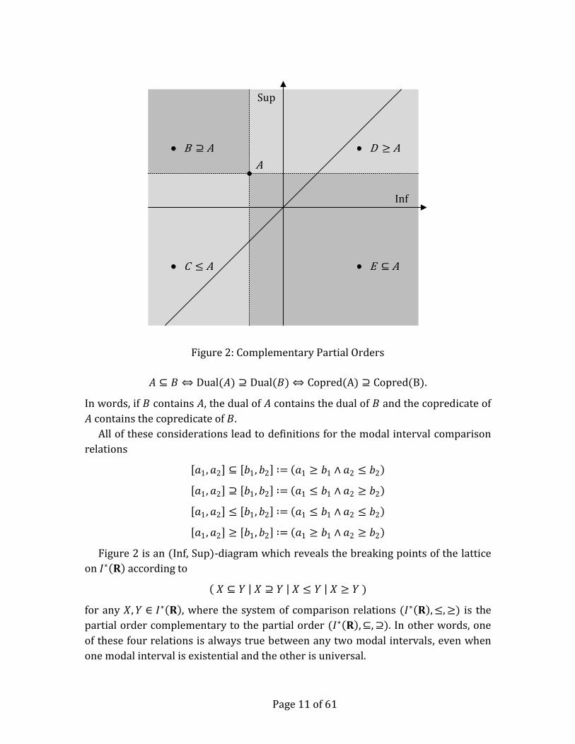
All of these considerations lead to definitions for the modal interval comparison

relations

𝑎1,𝑎2 ⊆ 𝑏1, 𝑏2 ∶= 𝑎1 ≥ 𝑏1 ∧ 𝑎2 ≤ 𝑏2

𝑎1,𝑎2 ⊇ 𝑏1, 𝑏2 ∶= 𝑎1 ≤ 𝑏1 ∧ 𝑎2 ≥ 𝑏2

𝑎1,𝑎2 ≤ 𝑏1, 𝑏2 ∶= 𝑎1 ≤ 𝑏1 ∧ 𝑎2 ≤ 𝑏2

𝑎1,𝑎2 ≥ 𝑏1, 𝑏2 ∶= 𝑎1 ≥ 𝑏1 ∧ 𝑎2 ≥ 𝑏2

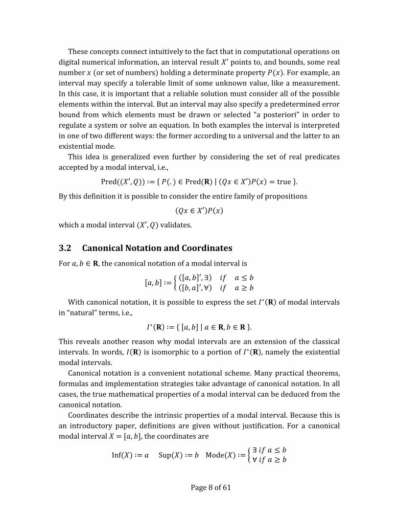
Figure 2 is an (Inf, Sup)-diagram which reveals the breaking points of the lattice

on 𝐼∗ 𝐑 according to

𝑋 ⊆ 𝑌 𝑋 ⊇ 𝑌 𝑋 ≤ 𝑌 𝑋 ≥ 𝑌 )

for any 𝑋,𝑌 ∈ 𝐼∗ 𝐑 , where the system of comparison relations (𝐼∗ 𝐑 ,≤,≥) is the

partial order complementary to the partial order (𝐼∗ 𝐑 ,⊆,⊇). In other words, one

of these four relations is always true between any two modal intervals, even when

one modal interval is existential and the other is universal.

Figure 2: Complementary Partial Orders

Sup

Inf

D ≥ AB ⊇ A

C ≤ A E ⊆ A

A

Page 12 of 61

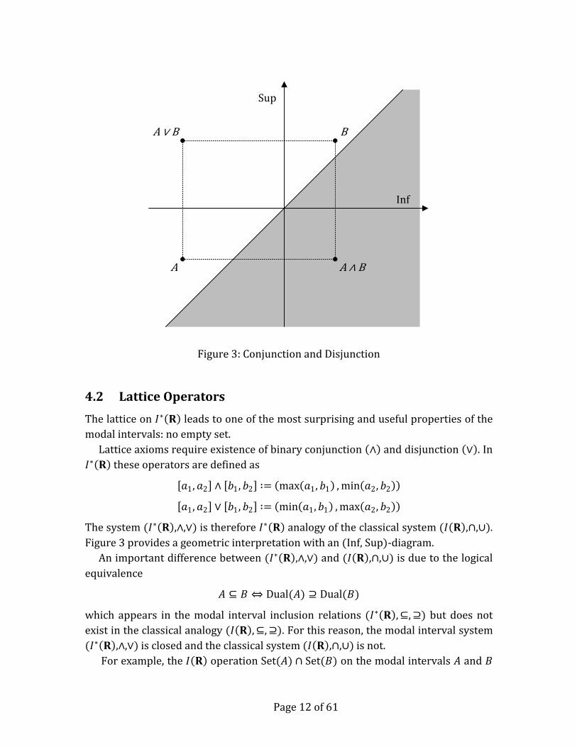
4.2 Lattice Operators

The lattice on 𝐼∗ 𝐑 leads to one of the most surprising and useful properties of the

modal intervals: no empty set.

Lattice axioms require existence of binary conjunction ∧ and disjunction ∨ . In

𝐼∗ 𝐑 these operators are defined as

𝑎1,𝑎2 ∧ 𝑏1, 𝑏2 ∶= max 𝑎1, 𝑏1 , min 𝑎2, 𝑏2

𝑎1,𝑎2 ∨ 𝑏1, 𝑏2 ∶= min 𝑎1,𝑏1 , max 𝑎2, 𝑏2

The system (𝐼∗ 𝐑 ,∧,∨) is therefore 𝐼∗ 𝐑 analogy of the classical system (𝐼 𝐑 ,∩,∪).

Figure 3 provides a geometric interpretation with an (Inf, Sup)-diagram.

An important difference between (𝐼∗ 𝐑 ,∧,∨) and (𝐼 𝐑 ,∩,∪) is due to the logical

equivalence

𝐴 ⊆ 𝐵 ⇔ Dual(𝐴) ⊇ Dual(𝐵)

which appears in the modal interval inclusion relations (𝐼∗ 𝐑 ,⊆,⊇) but does not

exist in the classical analogy (𝐼 𝐑 ,⊆,⊇). For this reason, the modal interval system

(𝐼∗ 𝐑 ,∧,∨) is closed and the classical system (𝐼 𝐑 ,∩,∪) is not.

For example, the 𝐼 𝐑 operation Set(𝐴) ∩ Set(𝐵) on the modal intervals 𝐴 and 𝐵

Figure 3: Conjunction and Disjunction

Sup

Inf

A

B

A ∧ B

A ∨ B

Page 13 of 61

depicted in Figure 3 is equivalent to the classical analogy of an intersection between

the disjoint set-theoretic intervals 𝐴′ and 𝐵′. In this case, 𝐴′ ∩ 𝐵′ ∉ 𝐼 𝐑 is the empty

set. The (Inf, Sup)-diagram reveals a geometric interpretation. The operation 𝐴′ ∩ 𝐵′

produces a result in the shaded area of the diagram representing invalid classical

intervals, i.e., the intervals which do not belong to the 𝐼 𝐑 system. By comparison,

𝐴 ∧ 𝐵 ∈ 𝐼∗ 𝐑 is a universal modal interval, which is a member of the 𝐼∗ 𝐑 system.

For this reason, the modal interval conjunction operator (∧) is closed.

This finding is often met with disbelief or received as a very shocking result of the

modal intervals, especially when one is accustomed to the classical intervals which

require an empty set. However, readers familiar with properties of convex duality

between points and planes in the study of oriented projective geometry may find the

equivalence of the relations

𝐴 ⊆ 𝐵 ⇔ Dual(𝐴) ⊇ Dual(𝐵),

as well as the closed and orderly structure of the system (𝐼∗ 𝐑 ,∧,∨), to be familiar

ideas. See, for example, “Oriented Projective Geometry, A Framework for Geometric

Computations,” Stolfi, Jorge, Academic Press, Inc., 1991, in which similar ideas and

concepts occur in the study of convex sets.

From a practical point of view, the closure of (𝐼∗ 𝐑 ,∧,∨) with respect to inclusion

means the empty set never appears in modal theory. This leads, however, to useful

computational abilities which will be explained in following sections. Any standard

aiming at modal interval compatibility does not need to provide an empty set for the

modal intervals, although such a standard may still provide an empty set for other

reasons. Classical interval algorithms such as interval Newton, for example, use the

empty set constructively in order to prove the non-existence of zeros. However, it is

also possible to modify the interval Newton method to prove non-existence of zeros

when universal intervals, and not empty intervals, are encountered.

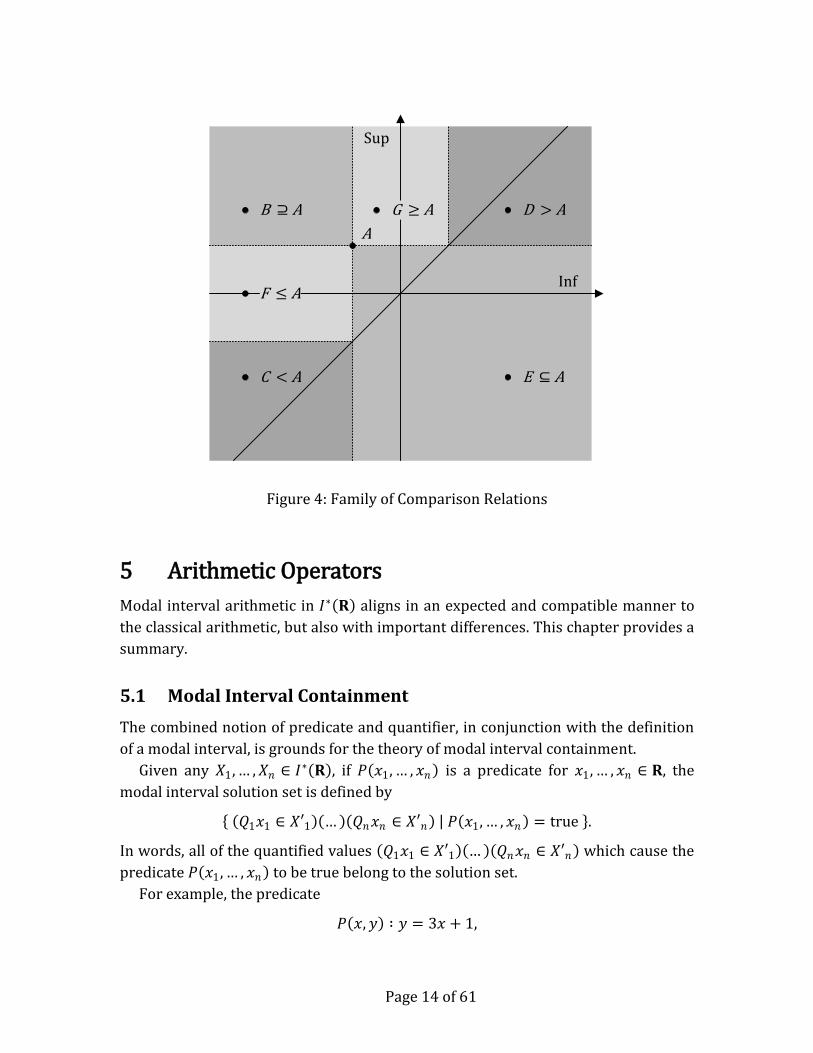
4.3 Strict Comparison Relations

In addition to the two partial orders (𝐼∗ 𝐑 ,≤,≥) and (𝐼∗ 𝐑 ,⊆,⊇), the strict modal

interval comparison relations are defined

𝑎1,𝑎2 < 𝑏1, 𝑏2 ∶= 𝑎1 < 𝑏1 ∧ 𝑎2 < 𝑏2 ∧ 𝑎1 < 𝑏2 ∧ 𝑎2 < 𝑏1

𝑎1,𝑎2 > 𝑏1, 𝑏2 ∶= 𝑎1 > 𝑏1 ∧ 𝑎2 > 𝑏2 ∧ 𝑎1 > 𝑏2 ∧ 𝑎2 > 𝑏1

Figure 4 shows the entire family of comparison relations for the modal interval 𝐴.

The relations 𝐶 < 𝐴 and 𝐷 > 𝐴 are the dark regions in the lower left and upper right

corners of the (Inf, Sup)-diagram. Note that two modal intervals 𝑋 and 𝑌 are disjoint

if 𝑋 < 𝑌 or 𝑋 > 𝑌.

Page 14 of 61

5 Arithmetic Operators

Modal interval arithmetic in 𝐼∗ 𝐑 aligns in an expected and compatible manner to

the classical arithmetic, but also with important differences. This chapter provides a

summary.

5.1 Modal Interval Containment

The combined notion of predicate and quantifier, in conjunction with the definition

of a modal interval, is grounds for the theory of modal interval containment.

Given any 𝑋1,… ,𝑋𝑛 ∈ 𝐼∗ 𝐑 , if 𝑃 𝑥1,… , 𝑥𝑛 is a predicate for 𝑥1,… , 𝑥𝑛 ∈ 𝐑, the

modal interval solution set is defined by

𝑄1𝑥1 ∈ 𝑋′1 … 𝑄𝑛𝑥𝑛 ∈ 𝑋′𝑛 𝑃 𝑥1,… , 𝑥𝑛 = true .

In words, all of the quantified values 𝑄1𝑥1 ∈ 𝑋′1 … 𝑄𝑛𝑥𝑛 ∈ 𝑋′𝑛 which cause the

predicate 𝑃 𝑥1,… , 𝑥𝑛 to be true belong to the solution set.

For example, the predicate

𝑃 𝑥,𝑦 ∶ 𝑦 = 3𝑥 + 1,

Figure 4: Family of Comparison Relations

Sup

Inf

D > AB ⊇ A

C < A E ⊆ A

A

F ≤ A

G ≥ A

Page 15 of 61

gives true propositions for some 𝑥,𝑦 ∈ 𝐑 and false propositions for the rest. The set

of all (𝑥,𝑦) pairs causing the predicate to be true forms a constraint, i.e., a graph of a

line. The predicate is false for any (𝑥,𝑦) pair not on the line because it violates the

constraint. The predicate therefore divides all (𝑥,𝑦) pairs into one of two sets, and

the set of all pairs for which the predicate is true is the solution set.

Note that the truth of a proposition of predicate 𝑃 𝑥,𝑦 depends on the quantifier

modes of 𝑥 and 𝑦. For example, the proposition

(∀𝑥 ∈ 𝐑)(∀𝑦 ∈ 𝐑)𝑃 𝑥,𝑦 ∶ 𝑦 = 3𝑥 + 1

is false because for any 𝑥 the predicate 𝑦 = 3𝑥 + 1 is not true for all 𝑦. However, the

proposition

(∀𝑥 ∈ 𝐑)(∃𝑦 ∈ 𝐑)𝑃 𝑥,𝑦 ∶ 𝑦 = 3𝑥 + 1

is true because for all 𝑥 there exists 𝑦 such that the predicate is true.

Modal theory generalizes these ideas to quantified interval equations. Given a

binary arithmetic operator ∘ and the real predicate 𝑃 𝑎, 𝑏, 𝑐 ∶ 𝑎 ∘ 𝑏 = 𝑐, the modal

interval equation 𝐴 ∘ 𝐵 = 𝐶 leads to one the following propositions

Proposition 1. ∀𝑎 ∈ 𝐴′ ∀𝑏 ∈ 𝐵′ ∃𝑐 ∈ 𝐶′ 𝑃 𝑎, 𝑏, 𝑐

Proposition 2. ∀𝑎 ∈ 𝐴′ 𝒬𝑐 ∈ 𝐶′ ∃𝑏 ∈ 𝐵′ 𝑃 𝑎, 𝑏, 𝑐

Proposition 3. ∀𝑏 ∈ 𝐵′ 𝒬𝑐 ∈ 𝐶′ ∃𝑎 ∈ 𝐴′ 𝑃 𝑎, 𝑏, 𝑐

Proposition 4. ∀𝑐 ∈ 𝐶′ ∃𝑏 ∈ 𝐵′ ∃𝑎 ∈ 𝐴′ 𝑃 𝑎, 𝑏, 𝑐

The scripted letter 𝒬 indicates the mode of 𝐶 depends on 𝐴 and 𝐵. Because “for all”

and “there exists” quantifiers are not generally commutative, an ordering problem

may arise. For this reason, only propositions with “for all” before “there exists” are

considered (and hence the re-ordering of the quantified variables).

The modal interval “Semantic Theorem for 𝑓*” then gives

min𝑎∈𝐴𝑏∈𝐵

𝑎 ∘ 𝑏 , max𝑎∈𝐴𝑏∈𝐵

𝑎 ∘ 𝑏 ⊆ 𝐶 ⇔ ∀𝑎 ∈ 𝐴′ ∀𝑏 ∈ 𝐵′ ∃𝑐 ∈ 𝐶′ 𝑃 𝑎, 𝑏, 𝑐

min𝑎∈𝐴

max𝑏∈𝐵

𝑎 ∘ 𝑏 , max𝑎∈𝐴

min𝑏∈𝐵

𝑎 ∘ 𝑏 ⊆ 𝐶 ⇔ ∀𝑎 ∈ 𝐴′ 𝒬𝑐 ∈ 𝐶′ ∃𝑏 ∈ 𝐵′ 𝑃 𝑎, 𝑏, 𝑐

min𝑏∈𝐵

max𝑎∈𝐴

𝑎 ∘ 𝑏 , max𝑏∈𝐵

min𝑎∈𝐴

𝑎 ∘ 𝑏 ⊆ 𝐶 ⇔ ∀𝑏 ∈ 𝐵′ 𝒬𝑐 ∈ 𝐶′ ∃𝑎 ∈ 𝐴′ 𝑃 𝑎, 𝑏, 𝑐

max𝑏∈𝐵𝑎∈𝐴

𝑎 ∘ 𝑏 , min𝑏∈𝐵𝑎∈𝐴

𝑎 ∘ 𝑏 ⊆ 𝐶 ⇔ ∀𝑐 ∈ 𝐶′ ∃𝑏 ∈ 𝐵′ ∃𝑎 ∈ 𝐴′ 𝑃 𝑎, 𝑏, 𝑐

These equivalences therefore provide both the mode and the range enclosure of any

arithmetic operation between two modal intervals.

Page 16 of 61

This shows the difference between modal and classical theory, i.e., the classical

theory is concerned only about the set-membership logic of Proposition 1. But this is

just one of several possible cases. Modal intervals are therefore an extension of the

classical intervals to the set-membership logic of all four cases. It is interesting to

note classical theory already uses the quantifiers, e.g., the real variables 𝑎, 𝑏 and 𝑐 in

Proposition 1 are quantified by universal and existential selection modes. Notation

styles in the classical literature do not always make this quantification explicit. But

even then the quantifier modes of Proposition 1 are assumed, i.e., they are implicit.

From a standards perspective, these are reasons why the modal and classical

approaches can be compatible.

Translation of Propositions 1-4 into formulas which can be easily implemented

inside a computer for the operations of addition, subtraction, multiplication and

division are given on p. 88 in the publication “Modal Intervals,” Gardenes, E. et. al.,

Reliable Computing 7.2, 2001, pp. 77-111. Addition and subtraction are trivial, and

multiplication and division are most efficiently implemented by creating a bit-mask

of the signs of the endpoints of the interval operands (the bit-mask can then be used

as an index into a single jump-table or switch statement).

It can also be shown modal intervals are isomorphic to the Kaucher intervals. As

an example, see Markov, S., “On Directed Interval Arithmetic and its Applications,”

Journal of Universal Computer Science 1.7, 1995, pp. 514-526. In an algebraic sense,

existential and universal modal intervals map to the proper and improper Kaucher

intervals. The operations of modal interval addition, subtraction, multiplication and

division then provide the same results as the Kaucher arithmetic, as do the lattice

operators and comparison relations.

5.2 Addition

In 𝐼 𝐑 , it is known that if 𝑎, 𝑏 ′ is a non-degenerate interval (𝑎 < 𝑏), there is no

interval 𝑥,𝑦 ′ such that

𝑎, 𝑏 ′ + 𝑥, 𝑦 ′ = 0,0 ′

and the equation

𝑎, 𝑏 ′ + 𝑥,𝑦 ′ = 𝑐, 𝑑 ′

has an interval solution only when 𝑏 − 𝑎 ≤ 𝑑 − 𝑐. Even in this case, the 𝐼 𝐑 -system

fails to obtain the solution from any set-theoretic interval operation between 𝑎, 𝑏 ′

and 𝑐,𝑑 ′.

For example, consider finding a solution for

1,2 ′ + 𝑥,𝑦 ′ = 3,5 ′

using the usual set-theoretic interval operations

Page 17 of 61

𝑥,𝑦 ′ = 3,5 ′ − 1,2 ′ = 1,4 ′.

In this case, addition has lost some of its group properties, i.e., the answer 1,4 ′ is

an overestimation of the correct answer 2,3 ′. Also, the lack of any solution to the

previously mentioned equation

𝑎, 𝑏 ′ + 𝑥, 𝑦 ′ = 0,0 ′

shows that no additive inverse element exists in 𝐼 𝐑 .

However, for any modal interval 𝑋,

𝑋 − Dual(𝑋) = 0,0

is an identity, i.e., the modal interval −Dual(𝑋) is the additive inverse element of 𝑋.

So the modal interval equation 𝐴 + 𝑋 = 𝐵 has the unique algebraic solution

𝑋 = 𝐵 − Dual(𝐴).

For example, consider an algebraic solution to the modal interval equation

1,3 + 𝑥,𝑦 = 0,0

using the modal interval operations

𝑥,𝑦 = 0,0 − Dual 1,3 = 0,0 − 3,1 = −1,−3 .

The answer is a universal modal interval. Substituting the answer into the original

equation results in

1,3 + −1,−3 = 0,0 .

For these reasons, modal interval addition is a group. In particular, it is abelian,

since the commutative property also holds. It can be shown containment is always

achieved even in the presence of directed rounding on floating-point numbers and

inexact results (see Section 5.4 of this paper).

5.3 Multiplication

As for addition, some of the group properties of multiplication in 𝐼 𝐑 are lost. For

example, consider finding a solution for

1,3 ′ ⋅ 𝑥,𝑦 ′ = 1,1 ′

using the usual set-theoretic interval operations

𝑥,𝑦 ′ = 1,1 ′/ 1,3 ′ = 1/3,1 ′.

Substituting the answer 1/3,1 ′ into the original equation yields

1,3 ′ ⋅ 1/3,1 ′ = 1/3,3 ′.

The interval 1/3,3 ′ is not equal to 1,1 ′, i.e., it is an overestimation of the right side

Page 18 of 61

of the original equation. The lack of an algebraic solution to the equation

1,3 ′ ⋅ 𝑥,𝑦 ′ = 1,1 ′

therefore shows no multiplicative inverse element exists in 𝐼 𝐑 . This is a reason the

distributive property in 𝐼 𝐑 is weakened and becomes a sub-distributive law

𝐴 ⋅ 𝐵 + 𝐶 ⊆ 𝐴 ⋅ 𝐵 + 𝐴 ⋅ 𝐶.

However, for any modal interval 𝑋 such that 0 ∉ Set(𝑋),

𝑋 Dual(𝑋) = 1,1

is an identity, i.e., the modal interval 1 Dual(𝑋) is the multiplicative inverse element

of 𝑋. The modal interval equation 𝐴 ⋅ 𝑋 = 𝐵 has the unique algebraic solution

𝑋 = 𝐵 Dual(𝐴)

so long as 0 ∉ Set(𝐴).

For example, consider an algebraic solution to the modal interval equation

1,3 ⋅ 𝑥,𝑦 = 1,1

using the modal interval operations

𝑥,𝑦 = 1,1 Dual 1,3 = 1,1 3,1 = 1,1/3 .

The answer is a universal modal interval. Substituting the answer into the original

equation results in

1,3 ⋅ 1,1/3 = 1,1 .

For these reasons, modal interval multiplication is a group for the set of all modal

intervals 𝑋 such that 0 ∉ Set(𝑋). In particular, it is abelian, since the commutative

property also holds. As for addition, it can be shown containment is always achieved

even in the presence of directed rounding on floating-point numbers and inexact

results (see Section 5.4 of this paper).

The sub-distributive property of 𝐼∗ 𝐑 therefore becomes much stronger than in

𝐼 𝐑 . Given the operators

Prop 𝑎, 𝑏 ∶= min 𝑎, 𝑏 , max(𝑎, 𝑏)

Impr 𝑎, 𝑏 ∶= max 𝑎, 𝑏 , min(𝑎, 𝑏)

the sub-distributive law in 𝐼∗ 𝐑 is

Impr 𝐴 ⋅ 𝐵 + 𝐴 ⋅ 𝐶 ⊆ 𝐴 ⋅ 𝐵 + 𝐶 ⊆ Prop 𝐴 ⋅ 𝐵 + 𝐴 ⋅ 𝐶.

For example,

1,3 ⋅ 1,1 + −1,−1 = 0,0 = 3,1 ⋅ 1,1 + 1,3 ⋅ −1,−1 .

This can be compared to the classical computation

Page 19 of 61

1,3 ′ ⋅ 1,1 ′ + 1,3 ′ ⋅ −1,−1 ′ = −2,2 ′.

As can be seen, the distributive property is stronger for modal intervals. All of the

valid distributive relations between modal intervals are many more than those for

the classical intervals, e.g., Popova, E. D., “Multiplication Distributivity of Proper and

Improper Intervals,” Reliable Computing 7.2, 2001, pp. 129-140.

5.4 Dual Computing Process

The “Dual Computing Process,” i.e., Theorem 4.5 in the 2001 reference by Gardenes

et. al., transforms the problem of finding an inner rounding of a numerical problem

into an equivalent computation that uses only the outer rounding.

Given Left 𝑥 ≤ 𝑥 and Right 𝑥 ≥ 𝑥 as the closest machine numbers adjacent to

the real number 𝑥, the outer and inner roundings are defined by

Out 𝑎, 𝑏 ∶= Left 𝑎 , Right 𝑏

Inn 𝑎, 𝑏 ∶= Right 𝑎 , Left 𝑏

The inner rounding of any interval arithmetic operation (∘) can then be computed

entirely in terms of outer rounding by

Inn 𝑋 ∘ 𝑌 ∶= Dual Out Dual 𝑋 ∘ Dual 𝑌 .

This is true since

Inn(𝑋) ⊆ 𝑋 ⊆ Out(𝑋),

which means the predicates of 𝑋 also satisfy the same inclusion relations (and the

copredicates satisfy in an antitonic manner). For this reason, the dual computing

process is an application of the logical equivalences

𝐴 ⊆ 𝐵 ⇔ Dual(𝐴) ⊇ Dual(𝐵) ⇔ Copred(A) ⊇ Copred(B),

which were presented earlier in Section 4.1 of this paper.

The dual computing process is important, because outward rounded data are not

always enough to obtain outward rounded results. For example, the exact equation

4/3,5/3 + 𝑥, 𝑦 = 2,7 ⇒ 𝑥,𝑦 = 2/3,16/3 .

But for Out 𝐴 + 𝑋 = 𝐵

1.3,1.7 + 𝑥, 𝑦 = 2,7 ⇒ 𝑥,𝑦 = 0.7,5.3 ,

which is not even the outer rounding of the exact result! For Inn 𝐴 + 𝑋 = 𝐵

1.4,1.6 + 𝑥, 𝑦 = 2,7 ⇒ 𝑥,𝑦 = 0.6,5.4 ,

which is the outer rounding of the exact result 2/3,16/3 .

From a standards perspective, this property of the modal intervals is a highly

Page 20 of 61

advantageous feature. Hardware vendors only need to provide an outer rounding on

interval processors, for example, and users can then compute inner estimations and

roundings of numerical problems via the dual computing process. The same is true

even in software implementations. An application of this property for computing the

inner estimation of a parametric solution set hull can be found in Popova, E. and W.

Kraemer, “Inner and Outer Bounds for Parametric Linear Systems,” Journal of

Computational and Applied Mathematics 199.2, 2007, 310-316.

The dual computing process is a consequence of the unique properties of 𝐼∗ 𝐑 ,

e.g., the logical equivalence

𝐴 ⊆ 𝐵 ⇔ Dual(𝐴) ⊇ Dual(𝐵),

which implies no empty set. These are reasons why an equivalent dual computing

process does not exist in 𝐼 𝐑 .

5.5 Arithmetic Facts

Kaucher interval arithmetic structure provides the algebraic completion of classical

interval arithmetic. The modal intervals, as mentioned previously, are isomorphism.

Summarizing, the following facts are relevant:

1. For any binary arithmetic operator (∘) and 𝐴,𝐵,𝐶,𝐷 ∈ 𝐼∗ 𝐑 ,

𝐴 ⊆ 𝐵,𝐶 ⊆ 𝐷 ⇒ 𝐴 ∘ 𝐶 ⊆ 𝐵 ∘ 𝐷.

2. For any two modal intervals, there always exists at least one true relation in

the system (𝐼∗ 𝐑 ,⊆,⊇,≤,≥).

3. (𝐼∗ 𝐑 ,∧,∨) is closed with respect to inclusion.

4. (𝐼∗ 𝐑 , +) is an abelian group.

5. For any 𝑋 ∈ 𝐼∗ 𝐑 , multiplicative inverse element 1 Dual(𝑋) exists so long as

0 ∉ Set(𝑋).

6. Multiplication is an abelian group for the set of all modal intervals with an

inverse element.

7. The distributive property in 𝐼∗ 𝐑 is stronger than in 𝐼 𝐑 .

8. The equation 𝐴 + 𝑋 = 𝐵 has a unique solution 𝑋 = 𝐵 − Dual(𝐴).

9. If 0 ∉ Set(𝐴), the equation 𝐴 ⋅ 𝑋 = 𝐵 has a unique solution 𝑋 = 𝐵 Dual(𝐴) .

10. The dual computing process requires only one mode of directed rounding to

compute both inner and outer estimations.

11. The modal interval comparison relations, as well as the lattice and arithmetic

operators, provide the same results as definitions provided by E. Kaucher for

intervals in the extended space of proper and improper intervals.

Modal intervals therefore provide an important connection between numeric and

Page 21 of 61

symbolic interval computations. For example, symbolic rearrangement of algebraic

expressions is an important application of computer science often ignored by the

classical interval community. This is due to the fact that classical intervals have no

group properties. However, modal intervals allow algebraic expressions to be safely

rearranged in compilers. They also provide foundation for robust Computer Algebra

Systems (CAS) that operate on algebraic expressions.

In the publication “Directed Interval Arithmetic in Mathematica: Implementation

and Applications,” Popova, E. D. and C. P. Ullrich, Technical Report 96-3, Universitaet

Basel, January 1996, the authors appeal to directed (modal) intervals:

Although conventional interval arithmetic is widely used in interval analysis

and has numerous applications, it possesses only few algebraic properties.

Lattice operations are not closed with respect to the inclusion relation. Due

to the lack of inverse elements with respect to the addition and

multiplication operations, the solution of the algebraic interval equations

𝐴 + 𝑋 = 𝐵 and 𝐴 ⋅ 𝑋 = 𝐵 cannot be generally expressed in terms of the

interval operations even if they actually exist. There is no distributivity

between addition and multiplication except for certain special cases. A

considerable scientific effort is put into developing special methods and

algorithms that try to overcome the difficulties imposed by the algebraic

incompleteness of the conventional interval arithmetic structure. For

example, arithmetic operations between conventional intervals can be used

for rough outer inclusion of functional ranges. But the bounds computed by

naïve interval evaluation are often too pessimistic to be useful. Again several

strategies have been developed to compute tighter bounds. Arithmetic

operations between conventional intervals are also of little use for the

computation of inner inclusions.

This outlines a distinction between “interval arithmetic” and “interval analysis.”

Popova points out how a great deal of effort is often spent trying to overcome the

incomplete structure of classical interval arithmetic, and this is a reference to

various interval analysis techniques in the interval literature.

From a standards perspective, this can be important to consider. It is without

doubt that interval analysis plays a crucial role in interval computations. But it is

also beyond the purview of a standard such as IEEE 1788 to standardize “interval

analysis” and not “interval arithmetic.”

For this reason, it is particularly relevant to consider the arithmetical properties

of intervals which are to be included in such a standard. Since the modal intervals

are the algebraic completion of the classical intervals, it is clear they provide the

most natural and reasonable choice.

People unfamiliar with the modal intervals may naturally resist this idea, but it

Page 22 of 61

should be remembered they are compatible, i.e., it is easy to perform purely classical

interval arithmetic with a modal interval datatype. If all inputs are existential, and if

no Dual(.) operators appear in the computation, the result coincides exactly with the

classical set-theoretic answer. The only exception is that conjunction (intersection)

of two disjoint intervals produces a universal interval. But this coincides with the

case where the classical operation provides an empty result, anyway. So it already

requires special handling in 𝐼 𝐑 .

5.6 Historical Context

The history of modal intervals goes back to the very first publications on the topic of

interval calculus. There are two papers considered as the pioneering works in this

field: one by Japanese mathematician T. Sunaga in 1958, and another by the Polish

mathematician M. Warmus in 1956. Both were apparently completed independent

of each other. In 1961, a second paper appeared by Warmus.

In the paper by Sunaga, almost all foundational elements of the interval calculus,

as known today, are presented. This includes the concept of the interval lattice 𝐼(𝐑),

the system of relations (𝐼 𝐑 ,⊆,⊇), the system of operators (𝐼 𝐑 ,∩,∪), the interval

arithmetic

𝑋 + 𝑌 = 𝑥 + 𝑦 𝑥 ∈ 𝑋,𝑦 ∈ 𝑌

𝑋 − 𝑌 = 𝑥 − 𝑦 𝑥 ∈ 𝑋,𝑦 ∈ 𝑌

𝑋𝑌 = 𝑥𝑦 𝑥 ∈ 𝑋,𝑦 ∈ 𝑌

𝑋 𝑌 = 𝑥 𝑦 𝑥 ∈ 𝑋,𝑦 ∈ 𝑌

and the sub-distributive law

𝐴 ⋅ 𝐵 + 𝐶 ⊆ 𝐴 ⋅ 𝐵 + 𝐴 ⋅ 𝐶.

Modal intervals are not formally developed, but in Example 3.4 on p. 32 of his paper,

Sunaga provides the interval 1,3 as the solution to the equation

1,2 + 𝑋 = 2,5 .

This is a remarkable anticipation of the formal (algebraic) solution provided by the

modal interval arithmetic, i.e.,

𝑋 = 2,5 − Dual 1,2 = 2,5 − 2,1 = 1,3 .

Perhaps even more remarkable, in the 1956 paper by Warmus, the system

𝐼∗ 𝐑 ∶= 𝑎, 𝑏 𝑎 ∈ 𝐑, 𝑏 ∈ 𝐑

is considered, along with the remark “there is now no need to assume 𝑎 ≤ 𝑏” for the

interval 𝑎, 𝑏 . Midpoint-radius form is also considered, and the sign of the radius is

Page 23 of 61

used to distinguish proper and improper intervals. He defines arithmetic operators

that provide inverse elements, noting the intervals then “form a ring with respect to

addition and regular multiplication.” He also points out that for system 𝐼∗ 𝐑 there

is “one-to-one correspondence between the approximate numbers, i.e., the intervals,

and the points on a plane.” This is a reference to geometric isomorphisms such as an

(Inf, Sup)-diagram, and in his 1961 paper he presents a graphical depiction in which

the entire plane is covered by the elements of 𝐼∗ 𝐑 . In this later paper he concludes

with an example

4,−2 ⋅ 𝑋 + −6,−2 ⊃ 0

which he rearranges into

4,−2 ⋅ 𝑋 ⊃ 6,2 .

This is equivalent to adding the modal interval inverse element −Dual −6,−2 to

both sides of the inequality!

Since the publications of Sunaga and Warmus, classical interval analysis has been

greatly popularized by Ramon E. Moore, who accomplished his dissertation on the

subject in 1962 and then published a monograph in 1966. Although less known, the

ideas of Sunaga and Warmus have also been advanced by others. Formal algebraic

properties of proper and improper intervals were independently studied in 1968 by

H. J. Ortolf and in 1973 by E. Kaucher. Inner arithmetic operations for the proper

intervals were developed in 1977 by S. Markov. In 1985, E. Gardenes conceived the

modal intervals, i.e., the grounding of modal analysis in predicate logic. In 1992, N.

Dimitrova, S. Markov and E. Popova studied important relations between Kaucher

intervals and inner operations on proper intervals. This work was later generalized

to the system of directed intervals in 1995 by S. Markov.

Directed intervals (S. Markov) coincide with the logical equivalences provided by

“Semantic Theorem for 𝑓*” in Propositions 1-4 (Gardenes, et. al.) presented earlier

in Section 5.1 of this paper. Directed intervals are also isomorphic to the Kaucher

intervals, as shown by S. Markov in 1995. For this reason, all prior investigations of

interval algebraic structures lead to a single system of interval arithmetic. Because

of the papers by T. Sunaga and M. Warmus, the modern view of the modal arithmetic

traces all the way back to the historical inception of the interval calculus. Most

remarkably, it is largely the same now as it was over fifty years ago.

6 Applications to Computer Graphics

This section of the paper presents an application of the modal interval analysis to

computer graphics and Computer Aided Design (CAD), namely the computation of

narrow bounds on Bezier and B-Spline curves.

Page 24 of 61

6.1 Polynomial and Rational Functions

A polynomial is a mathematical function involving the sum of powers of a function

variable, 𝑥, multiplied by coefficients 𝑎0, 𝑎1, 𝑎2, …, 𝑎𝑛 . A polynomial has the general

analytic form

𝑓 𝑥 = 𝑎𝑛𝑥𝑛 + ⋯+ 𝑎2𝑥

2 + 𝑎1𝑥 + 𝑎0.

The degree of a polynomial is the number 𝑛 characterizing the largest power of the

polynomial. The ratio of two polynomial functions is called a rational function. If

𝑓 𝑥 and 𝑔 𝑥 are two polynomial functions, then

𝑕 𝑥 =𝑓(𝑥)

𝑔(𝑥)

is a rational function.

The most efficient method to evaluate a polynomial function is by using Horner’s

rule, which factors out powers of 𝑥, giving

𝑓 𝑥 = 𝑎𝑛𝑥 + 𝑎𝑛−1 𝑥 + ⋯ 𝑥 + 𝑎0.

This method minimizes the number of arithmetical operations and results in less

numerical instability than a more naïve computational approach.

Although Horner’s rule is the most computationally efficient method to evaluate a

polynomial function, it has several disadvantages. Namely, the coefficients of the

polynomial have little geometric relation to the shape of the curve, and the method

is not numerically stable if the coefficients vary greatly in magnitude.

6.2 Bezier Curves

Popular and ubiquitous applications such as desktop publishing, computer graphics,

and Computer Aided Design (CAD) put the focus on interactive shape design, that is,

the emphasis of the polynomial computations are geometric in nature. This is in

contrast to the “algebraic flavor” of Horner’s rule and the analytic form of a

polynomial as previously presented.

For these reasons, alternative computational methods for polynomials were

developed in the 1960’s. These innovations were due largely to competition in the

automotive industry, occurring over a period of time when the availability of

computers and CAD software was replacing traditional paper and pencil design

methods. The breakthrough insight was to use control polygons, a technique that

was never used before. The polynomial is defined such that the coefficients are the

control points of a control polygon. This innovation greatly facilitates interactive

shape design, as changes to the control polygon cause the polynomial curve to

follow in a very intuitive way.

Page 25 of 61

To this day, such polynomial forms are known simply as “Bezier curves,” after

Pierre Bezier, the mathematician who first published them. Evaluating a point on a

Bezier curve can be done by a process similar to Horner’s rule. The method was

developed by Paul de Casteljau, and it uses recursive linear interpolation of control

points of a control polygon of a Bezier curve.

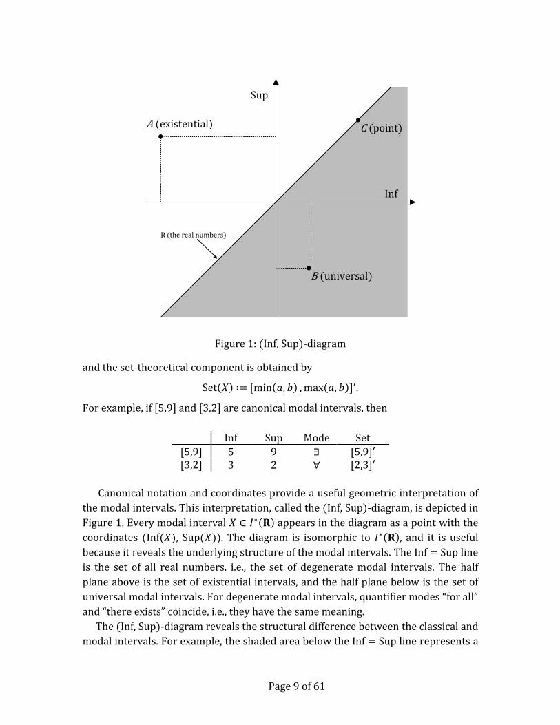
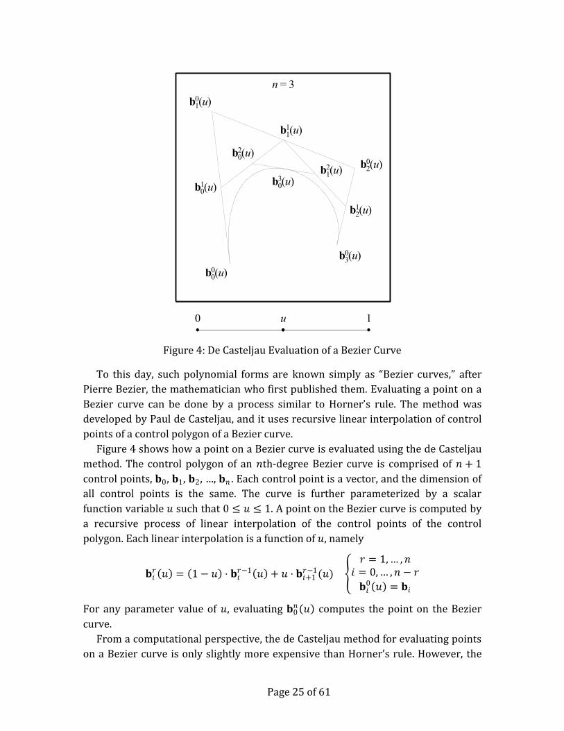
Figure 4 shows how a point on a Bezier curve is evaluated using the de Casteljau

method. The control polygon of an 𝑛th-degree Bezier curve is comprised of 𝑛 + 1

control points, 𝐛0, 𝐛1, 𝐛2, …, 𝐛𝑛 . Each control point is a vector, and the dimension of

all control points is the same. The curve is further parameterized by a scalar

function variable 𝑢 such that 0 ≤ 𝑢 ≤ 1. A point on the Bezier curve is computed by

a recursive process of linear interpolation of the control points of the control

polygon. Each linear interpolation is a function of 𝑢, namely

𝐛𝑖𝑟 𝑢 = 1 − 𝑢 ⋅ 𝐛𝑖

𝑟−1 𝑢 + 𝑢 ⋅ 𝐛𝑖+1𝑟−1(𝑢)

𝑟 = 1,… ,𝑛𝑖 = 0,… ,𝑛 − 𝑟

𝐛𝑖0 𝑢 = 𝐛𝑖

For any parameter value of 𝑢, evaluating 𝐛0𝑛 𝑢 computes the point on the Bezier

curve.

From a computational perspective, the de Casteljau method for evaluating points

on a Bezier curve is only slightly more expensive than Horner’s rule. However, the

Figure 4: De Casteljau Evaluation of a Bezier Curve

0 1u

b00(u)

b10(u)

b20(u)

b30(u)

b01(u)

b11(u)

b21(u)

b02(u)

b12(u)

b03(u)

n = 3

Page 26 of 61

de Casteljau method is more numerically stable. These qualities, as well as their

geometric nature, are the main reason why the Bezier curve and the de Casteljau

method are so common and ubiquitous in geometric applications such as desktop

publishing, computer graphics and CAD.

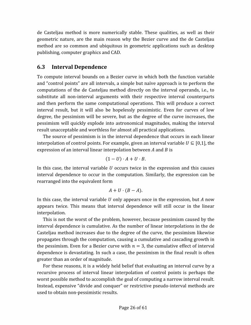
6.3 Interval Dependence

To compute interval bounds on a Bezier curve in which both the function variable

and “control points” are all intervals, a simple but naïve approach is to perform the

computations of the de Casteljau method directly on the interval operands, i.e., to

substitute all non-interval arguments with their respective interval counterparts

and then perform the same computational operations. This will produce a correct

interval result, but it will also be hopelessly pessimistic. Even for curves of low

degree, the pessimism will be severe, but as the degree of the curve increases, the

pessimism will quickly explode into astronomical magnitudes, making the interval

result unacceptable and worthless for almost all practical applications.

The source of pessimism is in the interval dependence that occurs in each linear

interpolation of control points. For example, given an interval variable 𝑈 ⊆ [0,1], the

expression of an interval linear interpolation between 𝐴 and 𝐵 is

1 − 𝑈 ⋅ 𝐴 + 𝑈 ⋅ 𝐵.

In this case, the interval variable 𝑈 occurs twice in the expression and this causes

interval dependence to occur in the computation. Similarly, the expression can be

rearranged into the equivalent form

𝐴 + 𝑈 ⋅ (𝐵 − 𝐴).

In this case, the interval variable 𝑈 only appears once in the expression, but 𝐴 now

appears twice. This means that interval dependence will still occur in the linear

interpolation.

This is not the worst of the problem, however, because pessimism caused by the

interval dependence is cumulative. As the number of linear interpolations in the de

Casteljau method increases due to the degree of the curve, the pessimism likewise

propagates through the computation, causing a cumulative and cascading growth in

the pessimism. Even for a Bezier curve with 𝑛 = 3, the cumulative effect of interval

dependence is devastating. In such a case, the pessimism in the final result is often

greater than an order of magnitude.

For these reasons, it is a widely held belief that evaluating an interval curve by a

recursive process of interval linear interpolation of control points is perhaps the

worst possible method to accomplish the goal of computing a narrow interval result.

Instead, expensive “divide and conquer” or restrictive pseudo-interval methods are

used to obtain non-pessimistic results.

Page 27 of 61

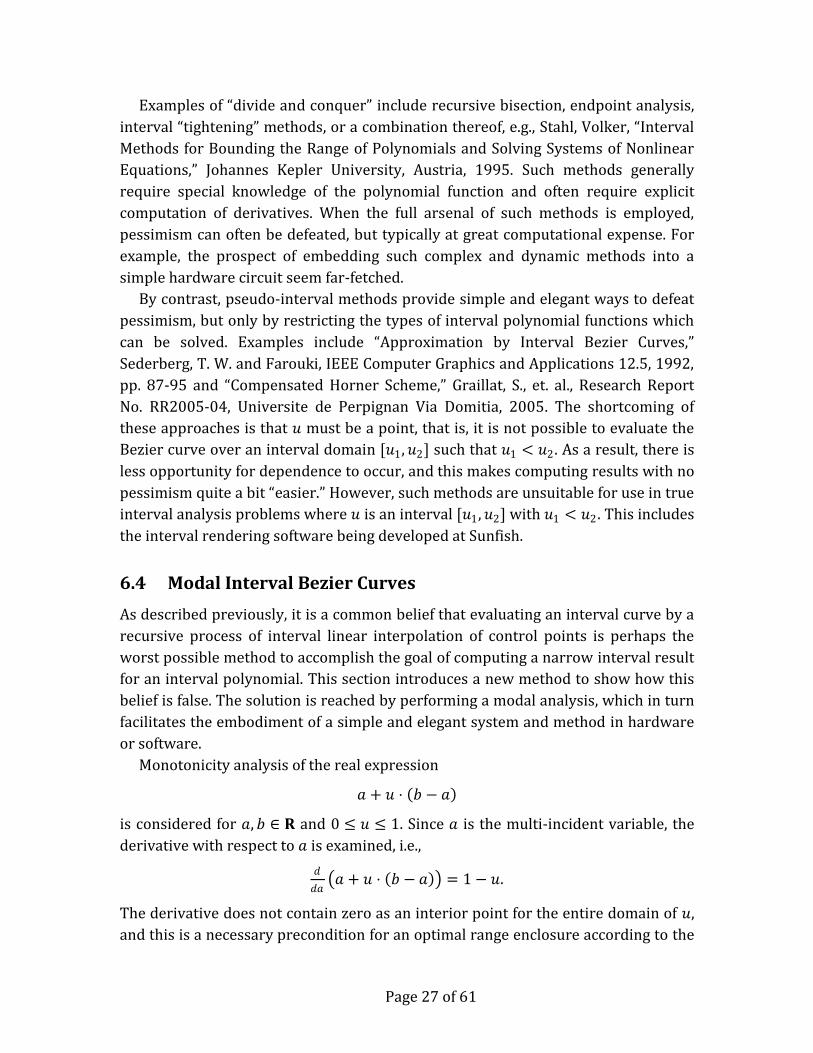
Examples of “divide and conquer” include recursive bisection, endpoint analysis,

interval “tightening” methods, or a combination thereof, e.g., Stahl, Volker, “Interval

Methods for Bounding the Range of Polynomials and Solving Systems of Nonlinear

Equations,” Johannes Kepler University, Austria, 1995. Such methods generally

require special knowledge of the polynomial function and often require explicit

computation of derivatives. When the full arsenal of such methods is employed,

pessimism can often be defeated, but typically at great computational expense. For

example, the prospect of embedding such complex and dynamic methods into a

simple hardware circuit seem far-fetched.

By contrast, pseudo-interval methods provide simple and elegant ways to defeat

pessimism, but only by restricting the types of interval polynomial functions which

can be solved. Examples include “Approximation by Interval Bezier Curves,”

Sederberg, T. W. and Farouki, IEEE Computer Graphics and Applications 12.5, 1992,

pp. 87-95 and “Compensated Horner Scheme,” Graillat, S., et. al., Research Report

No. RR2005-04, Universite de Perpignan Via Domitia, 2005. The shortcoming of

these approaches is that 𝑢 must be a point, that is, it is not possible to evaluate the

Bezier curve over an interval domain [𝑢1,𝑢2] such that 𝑢1 < 𝑢2 . As a result, there is

less opportunity for dependence to occur, and this makes computing results with no

pessimism quite a bit “easier.” However, such methods are unsuitable for use in true

interval analysis problems where 𝑢 is an interval [𝑢1,𝑢2] with 𝑢1 < 𝑢2 . This includes

the interval rendering software being developed at Sunfish.

6.4 Modal Interval Bezier Curves

As described previously, it is a common belief that evaluating an interval curve by a

recursive process of interval linear interpolation of control points is perhaps the

worst possible method to accomplish the goal of computing a narrow interval result

for an interval polynomial. This section introduces a new method to show how this

belief is false. The solution is reached by performing a modal analysis, which in turn

facilitates the embodiment of a simple and elegant system and method in hardware

or software.

Monotonicity analysis of the real expression

𝑎 + 𝑢 ⋅ 𝑏 − 𝑎

is considered for 𝑎, 𝑏 ∈ 𝐑 and 0 ≤ 𝑢 ≤ 1. Since 𝑎 is the multi-incident variable, the

derivative with respect to 𝑎 is examined, i.e.,

𝑑

𝑑𝑎 𝑎 + 𝑢 ⋅ 𝑏 − 𝑎 = 1 − 𝑢.

The derivative does not contain zero as an interior point for the entire domain of 𝑢,

and this is a necessary precondition for an optimal range enclosure according to the

Page 28 of 61

modal analysis. Next, each instance of 𝑎 is treated as an independent variable, e.g.,

𝑎0 + 𝑢 ⋅ 𝑏 − 𝑎1 ,

each instance 𝑎0 and 𝑎1 an independent variable, and the derivatives

𝑑

𝑑𝑎0 𝑎0 + 𝑢 ⋅ 𝑏 − 𝑎1 = 1 and

𝑑

𝑑𝑎1 𝑎0 + 𝑢 ⋅ 𝑏 − 𝑎1 = −𝑢

are examined. The derivatives with respect to 𝑎0 and 𝑎1 have opposite signs, and the

instance 𝑎0 shares the same sign in the derivative as 𝑎 (the instance 𝑎1 does not). In

the publication “Modal Intervals,” Gardenes, E. et. al., Reliable Computing 7.2, 2001,

pp. 77-111, by Theorem 5.4, i.e., by the “Coercion to Optimality,” the instance 𝑎1 is

therefore dualized and the interval linear interpolation becomes

𝐴 + 𝑈 ⋅ (𝐵 − Dual(𝐴)).

In other words, the linear interpolation operation is now an optimal modal interval

expression.

This optimal form of the interval linear interpolation cannot be overemphasized.

It is a total defeat of interval dependence as discussed in the previous section. Most

importantly, since 𝑈 ⊆ [0,1] is true for every step of the de Casteljau method, it can

be used recursively to compute narrow bounds on an interval Bezier curve.

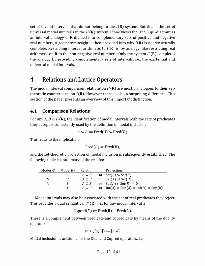
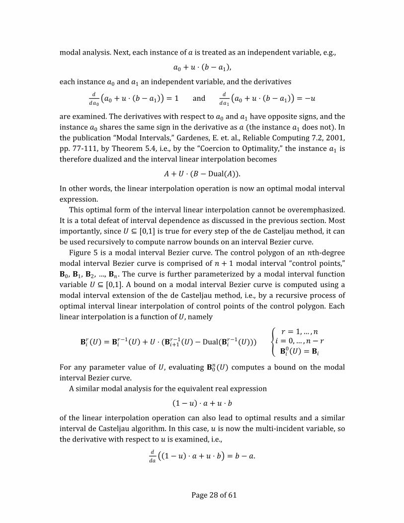
Figure 5 is a modal interval Bezier curve. The control polygon of an 𝑛th-degree

modal interval Bezier curve is comprised of 𝑛 + 1 modal interval “control points,”

𝐁0, 𝐁1, 𝐁2, …, 𝐁𝑛 . The curve is further parameterized by a modal interval function

variable 𝑈 ⊆ [0,1]. A bound on a modal interval Bezier curve is computed using a

modal interval extension of the de Casteljau method, i.e., by a recursive process of

optimal interval linear interpolation of control points of the control polygon. Each

linear interpolation is a function of 𝑈, namely

𝐁𝑖𝑟 𝑈 = 𝐁𝑖

𝑟−1 𝑈 + 𝑈 ⋅ (𝐁𝑖+1𝑟−1 𝑈 − Dual(𝐁𝑖

𝑟−1(𝑈)))

𝑟 = 1,… ,𝑛𝑖 = 0,… ,𝑛 − 𝑟

𝐁𝑖0 𝑈 = 𝐁𝑖

For any parameter value of 𝑈, evaluating 𝐁0𝑛(𝑈) computes a bound on the modal

interval Bezier curve.

A similar modal analysis for the equivalent real expression

1 − 𝑢 ⋅ 𝑎 + 𝑢 ⋅ 𝑏

of the linear interpolation operation can also lead to optimal results and a similar

interval de Casteljau algorithm. In this case, 𝑢 is now the multi-incident variable, so

the derivative with respect to 𝑢 is examined, i.e.,

𝑑

𝑑𝑎 1 − 𝑢 ⋅ 𝑎 + 𝑢 ⋅ 𝑏 = 𝑏 − 𝑎.

Page 29 of 61

However in this case zero may be an interior point in the derivative, so the modal

analysis requires branch conditions. For this reason it is not the preferred method,

e.g., it does not lead to the most efficient implementations. Nevertheless, it is an

obvious alternative that can lead to similar results.

In either case, the modal interval formulation of a Bezier curve is simple enough

that it can be easily implemented as a dedicated hardware circuit. If a modal interval

processor is available, the optimal interval linear interpolations can be managed by

a simple memory addressing unit and the modal interval arithmetic can be deeply

pipelined. If a modal interval processor is not available, it is easy to emulate by

disassembling the modal arithmetic into elementary floating-point operations and

then providing an appropriate sequence of machine instructions to a floating-point

processor. Emulation in software can also be achieved by using similar strategies.

All of these implementation choices follow naturally as a consequence of the modal

analysis.

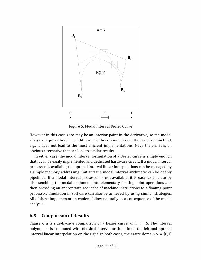
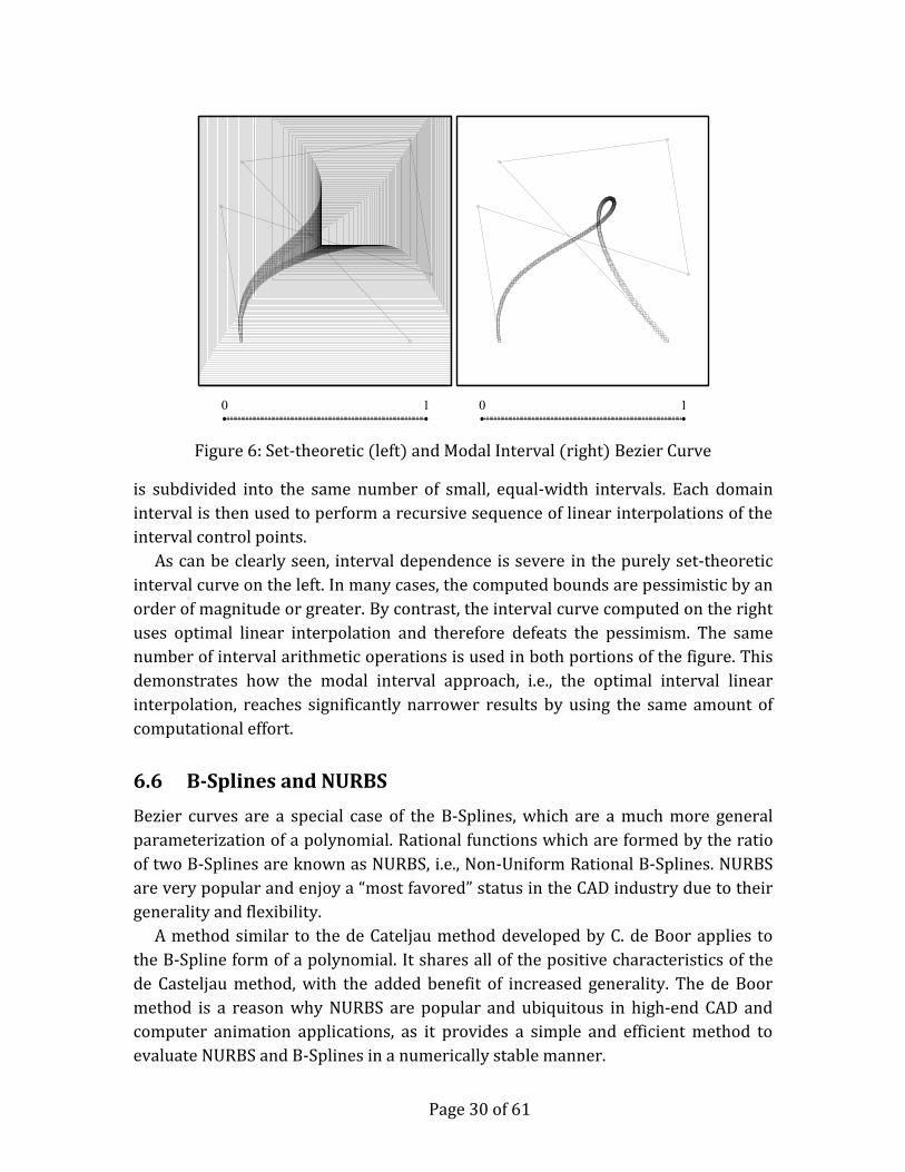
6.5 Comparison of Results

Figure 6 is a side-by-side comparison of a Bezier curve with 𝑛 = 5. The interval

polynomial is computed with classical interval arithmetic on the left and optimal

interval linear interpolation on the right. In both cases, the entire domain 𝑈 = [0,1]

Figure 5: Modal Interval Bezier Curve

0 1[ ]U

n = 3

B0

B1

B2

B3

B03(U)

Page 30 of 61

is subdivided into the same number of small, equal-width intervals. Each domain

interval is then used to perform a recursive sequence of linear interpolations of the

interval control points.

As can be clearly seen, interval dependence is severe in the purely set-theoretic

interval curve on the left. In many cases, the computed bounds are pessimistic by an

order of magnitude or greater. By contrast, the interval curve computed on the right

uses optimal linear interpolation and therefore defeats the pessimism. The same

number of interval arithmetic operations is used in both portions of the figure. This

demonstrates how the modal interval approach, i.e., the optimal interval linear

interpolation, reaches significantly narrower results by using the same amount of

computational effort.

6.6 B-Splines and NURBS

Bezier curves are a special case of the B-Splines, which are a much more general

parameterization of a polynomial. Rational functions which are formed by the ratio

of two B-Splines are known as NURBS, i.e., Non-Uniform Rational B-Splines. NURBS

are very popular and enjoy a “most favored” status in the CAD industry due to their

generality and flexibility.

A method similar to the de Cateljau method developed by C. de Boor applies to

the B-Spline form of a polynomial. It shares all of the positive characteristics of the

de Casteljau method, with the added benefit of increased generality. The de Boor

method is a reason why NURBS are popular and ubiquitous in high-end CAD and

computer animation applications, as it provides a simple and efficient method to

evaluate NURBS and B-Splines in a numerically stable manner.

Figure 6: Set-theoretic (left) and Modal Interval (right) Bezier Curve

0 1 0 1

Page 31 of 61

The modal interval methods and techniques described in this paper generalize

trivially to B-Splines and NURBS.

6.7 Comparison with Classical Approaches

Classical endpoint analysis for the real expression

𝑎 + 𝑢 ⋅ 𝑏 − 𝑎

also examines the derivative with respect to 𝑎, i.e.,

𝑑

𝑑𝑎 𝑎 + 𝑢 ⋅ 𝑏 − 𝑎 = 1 − 𝑢.

In this case, since the derivative is non-negative for the entire domain of 𝑢, the lower

and upper bound of 𝑎 can be used, respectively, in the lower and upper evaluation of

the range enclosure, i.e.,

Inf(Inf(𝐴) + 𝑈 ⋅ (𝐵 − Inf(𝐴))), Sup(Sup(𝐴) + 𝑈 ⋅ (𝐵 − Sup(𝐴))) .

This leads to the same optimal result as the modal analysis. However, it requires six

interval arithmetic operations, i.e., twice the number of operations required for the

modal interval expression

𝐴 + 𝑈 ⋅ (𝐵 − Dual(𝐴)),

which requires only three.

In any case, for an expression as simple as the linear interpolation operation, it

should not come as a surprise that classical endpoint analysis arrives at the same

range enclosure. Modal intervals are an extension of the classical intervals, and the

coercion theorems are based on monotonicity analysis. For these reasons, a modal

analysis includes traditional methods, such as classical endpoint analysis, as obvious

and alternative paths to the same destination.

In regards to computing narrow bounds on interval polynomials by using optimal

interval linear interpolation, however, there is not a prior solution, either classical

or modal, in the literature. There are also no publications, which we are aware of,

that discuss or show how to perform an optimal interval linear interpolation. We

believe optimal interval linear interpolation, either classical or modal, and its use in

recursive methods to compute narrow bounds on interval polynomials are unique

contributions to the interval community.

6.8 Linear Interpolation in the Vienna Proposal

It has been suggested in the public forum by Arnold Neumaier that optimal linear

interpolation does not require modal intervals. For set-theoretic intervals xx, yy and

tt, the optimal modal interval linear interpolation xx+tt*(yy-dual(xx)) is replaced

Page 32 of 61

by the library routine linearInt(xx,yy,tt), which uses the following recipe:

set round down dl = yl-xl; tl1=(tl if dl>=0 else tu); l=xl+tl1*dl; set round up du = yu-xu; tu1=(tu if du>=0 else tl); u=xu+tu1*du;

The inclusion of the linearInt() recipe in Version 3.0 of the Vienna Proposal, Nov.

21, 2008, was motivated by personal discussions on the topic of modal intervals and

optimal linear interpolation with Neumaier.

Following the obvious course mentioned at the end of Section 6.4 of this paper,

Neumaier obtains the linearInt() recipe (personal communication) from Hayes,

Nathan T., “System and Method to Compute Narrow Bounds on a Modal Interval

Polynomial Function,” Pub. No. WO/2007/041523, by disassembling the modal

interval arithmetic xx+tt*(yy-dual(xx)) into elementary floating-point operations!

For example,

[dl,du] = [yl-xl,yu-xu] = yy-dual(xx).

Similarly, the values of tl1 and tu1 in the linearInt() recipe come from the modal

interval multiplication table shown on p. 88 of Gardenes, E. et. al., “Modal Intervals,”

Reliable Computing 7.2, 2001, pp. 77-111. For example, since tt is a non-negative

interval, the modal interval multiplication tt*[dl,du] depends only on the signs of

dl and du. This means

[tl1*dl,tu1*du] = tt*[dl,du].

The addition of xl and xu in the lower and upper bounds of the linearInt() recipe,

respectively, follows from the interval addition operation, also depicted on p. 88 of

the Gardenes reference. In words, Neumaier simply rewrites the modal interval

expression in component-wise form.

Classical endpoint analysis does not disassemble into the same efficient recipe as

the modal analysis (see, for example, Section 6.7 of this paper). In the publication

“Computer graphics, linear interpolation and nonstandard intervals,” Dec. 22, 2008,

Neumaier provides an “a posteriori” change to a classical endpoint analysis to obtain

more efficient computation. But this change, i.e., the linearInt() recipe, is simply

the component-wise form of the modal interval arithmetic.

For example, a compiler can also disassemble the expression

𝐴 + 𝑈 ⋅ (𝐵 − Dual(𝐴))

into elementary floating-point operations and automatically obtain the linearInt()

recipe. Expert use of programming languages, such as C++ expression templates,

can also lead to similar results.

All of this shows why modal intervals may provide a fantastic opportunity for

advancements in linguistic interval technologies such as compilers or programming

Page 33 of 61

languages, e.g., a compiler or C++ class library may disassemble the modal interval

arithmetic to automatically obtain an optimal sequence of elementary operations for

a floating-point processor. Contrary to his claim, however, Neumaier demonstrates

that optimal linear interpolation does require modal intervals. In words, the most

efficient implementation is obtained directly from the modal arithmetic. Prohibiting

standardization of a modal interval datatype and requiring the linearInt() recipe,

as suggested in the Vienna Proposal, does not change this fact.

7 Modal Interval Schema

Modal intervals are an interval extension of the real numbers. Efforts to generalize

to the extended reals have been made by Miguel A. Sainz (personal communication)

and other mathematicians, e.g., E. Popova (1994), S. Markov (1996) and E. Popova

and C. Ullrich (1997).

An unresolved question in the modal interval literature is how to handle the IEEE

754 infinities in a practical implementation of modal intervals inside a computer.

These issues have been studied at Sunfish. We take the approach that infinities are

not allowed to be members of the modal interval.

This section summarizes an extension of modal intervals to the set of unbounded

modal intervals, along with a suitable schema for a practical implementation within

a computer. It compares in spirit to the purely set-theoretic schema presented in the

monograph “Self-Validated Numerical Methods and Applications,” Stolfi, Jorge and L.

H. de Figueirdedo, Brazilian Mathematics Colloquium, IMPA, Rio de Janeiro, Brazil,

1997. But the new schema presented in this chapter provides reliable and efficient

overflow tracking for unbounded modal intervals that do not contain infinites as

members. This schema is a prototype, and likely requires further development.

7.1 Background

Translating interval mathematics into practical computational methods that can be

performed within a computer is the purpose of the P1788 working group. IEEE 754

specifies exceptionally particular semantics for binary floating-point arithmetic and

enjoys pervasive and worldwide use in modern computer hardware. For this reason,

efforts focus on creating practical interval arithmetic implementations that build on

the reputation and legacy of this standard.

IEEE 754 specifies bit-patterns to represent real floating-point numbers as well

as +∞, −∞, −0, +0 and the pseudo-numbers, i.e., NaNs (Not-a-Number). Although

the standard defines results for the arithmetical combination of all permutations of

bit-patterns between two floating-point values, the translation of these results into

arithmetical combinations of intervals is unclear. This problem was first posed in

Page 34 of 61

Popova, E. D., “Extended Interval Arithmetic in IEEE Floating-Point Environment,”

Interval Computations, No. 4, 1994, pp. 100-129, and a model that makes IEEE 754

floating-point arithmetic and interval arithmetic compliant is presented.

Several efforts to map IEEE 754 to set-theoretic intervals have been made. In the

previously cited monograph, Stolfi presents a mapping to the real numbers. A more

ambitious mapping to the extended-reals is made by Walster in U.S. Pat. 6,658,443.

More recently, Steele, Jr. provides alternate results for invalid IEEE 754 arithmetic

operations in U.S. Pat. 7,069,288. For example, Steele defines

+∞ + −∞ = +∞

when rounding towards positive infinity and

+∞ + −∞ = −∞

when rounding in the opposite direction. In words, the alternate results depend on

rounding mode. These methods are not compatible with modal intervals, so a new

representation is needed.

7.2 Digital Scales

The set of real numbers 𝐑 is uncountable, so computers must therefore perform

calculations upon a finite subset of 𝐑. A digital scale is such a subset. Each mark in a

digital scale is represented in a computer by a bit-pattern and corresponds to a

particular element of 𝐑. Due to its finite nature, every digital scale is characterized

by a mark which represents a largest and a smallest real number.

Arithmetic operations performed on a digital scale may result in a number that is

not representable by any mark. If this occurs, the result is “correctly rounded” if the

exact answer is rounded to the nearest mark according to some specified rounding

convention. In interval arithmetic, two rounding conventions are used, i.e., round

down (towards negative infinity) and round up (towards positive infinity).

Overflow is a condition that occurs when a result of an arithmetic operation

exceeds the largest or smallest mark of the digital scale. To help track overflow in a

reliable manner, a digital scale can specify the two special marks −∞ and +∞ to

represent, respectively, overflow of the smaller or larger end of the digital scale.

More specifically, in IEEE 754 the marks −∞ and +∞ represent true infinite values,

i.e., they are not real numbers.

7.3 Bounded Modal Intervals

In a computer, a modal interval is comprised of a first and a second mark of a digital

scale. If both marks are real numbers, the set-theoretic component of the modal

interval is the closed set of all real numbers between and including the marks. The

Page 35 of 61

quantifier mode is deduced by the relative signed magnitude of the two marks. If the

first mark is less-than the second mark, the quantifier is existential. If the first mark

is greater-than the second mark, the quantifier is universal. If the two marks are

equal, the modal interval is a point and it represents a single real number with a

degenerate quantifier, i.e., the quantifiers “for all” and “there exists” have the same

meaning when the modal interval is a point.

7.4 Unbounded Modal Intervals

Prior methods of overflow tracking for modal intervals have been considered in the

literature, e.g., the previously mentioned references by Popova and Markov. We take

a different approach in which infinities are not allowed to be members of the modal

interval. The method presented here was developed several years ago at Sunfish

and has been used with success in practical implementations. It begins with the

introduction and treatment of unbounded modal intervals.

An unbounded modal interval is represented by a first and a second mark of a

digital scale, where at least one mark is a signed infinity, i.e., −∞ or +∞.

Strictly speaking, the presence of infinity in an unbounded modal interval is a

token which indicates an open and unbounded endpoint. The actual infinity is not

contained in the modal interval, but all real numbers 𝑥 approaching the infinity in

the limit are. For this reason, the unbounded modal interval is different from the

“extended-real” modal interval. The former contains only real numbers, while the

latter contains the infinity, which is not a real number. For example, the canonical

modal interval (−∞, 5] contains all real numbers 𝑥 ≤ 5 but not the infinity.

7.5 Special Modal Intervals

If both marks of a modal interval are infinities of the same sign, the modal interval is

a “point in the limit.” More specifically, the modal interval is a real number 𝑥 that

approaches infinity in the limit. The infinity approached by 𝑥 is the same as the two

endpoints of the interval. For example,

(+∞, +∞)

represents a real number 𝑥 in the limit as it approaches +∞, and

(−∞,−∞)

represents a real number 𝑥 in the limit as it approaches −∞. As is the case with all

points, the quantifier of a “point in the limit” is degenerate.

Other special modal intervals are the intervals comprising at least one signed

zero. IEEE 754 specifies distinct marks for −0 and +0, which are both aliases for

true mathematical zero. For this reason, zero has four aliases in the modal interval

Page 36 of 61

schema, i.e., one for each pair of zeros having one of the four possible permutations

of signs. All four aliases are points and have the same degenerate quantifier. As

should be obvious, this also means a bounded or unbounded modal interval which

contains the mark −0 or +0 in one endpoint is an alias for the same modal interval

with a zero of complimentary sign located in the same position, e.g., [−12,−0] and

[−12, +0] are aliases of each-other.

7.6 Indefinite Modal Intervals

So far, the modal interval schema has assigned a meaning for every permutation of

bit-pattern between two marks of a digital scale selected from the group of finite

real numbers, signed infinities and signed zeros. IEEE 754 also defines the pseudo-

numbers, called NaNs (Not-a-Number). If at least one mark of a modal interval is a

NaN, then the modal interval is indefinite or NaI (Not-an-Interval).

Indefinite modal intervals serve the same purpose as the NaNs do in IEEE 754,

i.e., they can be used to propagate errors through a computation. If a modal interval

operand is indefinite, the result of any lattice or arithmetic operation on it must also

be indefinite. It is always true that an indefinite modal interval is not equal to itself

or any other modal interval. All other comparison relations on an indefinite modal

interval are false.

Note that an indefinite interval is not the same as an empty interval, as the two

generally have different properties. For example, if 𝑋′ ∈ 𝐼(𝐑) is a classical interval,

then

𝑋′ ∪ ∅ = 𝑋′.

But if NaI is an indefinite interval, then

𝑋′ ∪ NaI = NaI.

Since modal intervals do not require the empty set, it is not specified in the schema.

However, classical interval algorithms can still operate properly with a modal

interval datatype by treating the universal intervals 𝑏,𝑎 such that 𝑏 > 𝑎 as empty

intervals. Consistent application of this rule always leads to the correct classical

results and allows the traditional interval algorithms such as the interval Newton

method to prove non-existence of zeros. For example, if all inputs to the algorithm

are existential intervals 𝑎, 𝑏 such that 𝑎 ≤ 𝑏, then any occurrence of a universal

interval is proof of non-existence of zeros.

7.7 Unbounded Addition

A complete mapping of IEEE 754 to the unbounded modal intervals has been given,

i.e., the schema has assigned meaning to every permutation of bit-pattern between

Page 37 of 61

two marks selected from the group of finite numbers, NaNs, signed infinities, and

signed zeros. This mapping provides representation for unbounded modal intervals.

The modal interval literature, however, provides no treatment of unbounded modal

intervals or how to perform arithmetic operations on them. What remains to be

done is to specify the operational semantics of unbounded modal intervals in the

context of modal interval arithmetic computations.

Consider an example of modal interval addition, 3, +∞ + (−∞, 2]. Semantically

speaking, this represents addition of two unbounded existential modal intervals.

IEEE arithmetic provides the result

3 + (−∞ , +∞) + 2 = (−∞, +∞).

Because the infinity in each operand represents a real number in the limit, the sums

of the endpoints are likewise real numbers in the limit. In this case, using IEEE

arithmetic to calculate the result provides the desired answer.

Consider a similar example where the modality of the first operand is universal,

i.e., +∞, 3 + (−∞, 2]. In this case, IEEE arithmetic provides the result

[ +∞) + −∞ , 3 + 2 = [NaN, 5].

The presence of NaN in the result is a consequence of an invalid operation. Namely,

the arithmetic operation (+∞) + (−∞) is invalid, and IEEE 754 specifies NaN as the

result. In this case, IEEE arithmetic does not work.

At this point, it is critically important to remember that due to the representation

of the present schema, the infinity is not actually contained in the modal interval. On

the contrary, it is in fact only a token to indicate a real number in the limit as it

approaches the infinity. This is in contrast to IEEE arithmetic, which does not treat

the infinity as a real number. It turns out that performing IEEE arithmetic directly

on the infinities in the first example provides the desired result. However, this is

only a fortunate coincidence. As the second example shows, such a computational

trick does not always provide the desired answer.

Remembering that the presence of infinities in a modal interval is only a token for

a real number in the limit as it approaches the infinity, a closer examination of the

two examples using substitution is helpful and revealing.

In the first example, substituting the infinite values for increasingly large real

magnitudes reveals the following trend

[3 + −1000 , +1000 + 2]

= [−997,1002]

[3 + −1000000 , +1000000 + 2]

= [−999997,1000002]

Page 38 of 61

[3 + −1000000000 , +1000000000 + 2]

= [−999999997,1000000002].

As larger and larger magnitudes are substituted for the infinite values, the sums

eventually overflow the digital scale, providing a result of (−∞, +∞) to represent an

unbounded interval. In this case, it is a coincidence that performing IEEE arithmetic

directly on the unbounded endpoints provides the desired result.

In the second example, substituting the infinite values for increasingly large real

magnitudes reveals the following trend

[ +1000 + −1000 , 3 + 2]

= [0,5]

[ +1000000 + −1000000 , 3 + 2]

= [0,5]

[ +1000000000 + −1000000000 , 3 + 2]

= [0,5].

As larger and larger magnitudes are substituted for the infinite values, the sums of

equal magnitude continually cancel each-other out, resulting in the modal interval

[0,5]. In this case, the computational trick of performing IEEE arithmetic directly on

the unbounded endpoints does not work.

As a conclusion to be drawn from these examples, it is a fortunate coincidence

that addition of unbounded modal intervals can be calculated using IEEE arithmetic

for any case where the result is not a NaN. Specifically, the exceptional conditions of

IEEE addition are (+∞) + (−∞) and (−∞) + (+∞). Special instruction is required

in these cases to return +0 as the proper result, except when rounding down the

result should be −0. Note the sign of the result coincides with the rules of IEEE 754

addition for finite numbers.

As it should be obvious, the same conclusion and results are obtained for the

subtraction of unbounded modal intervals.

7.8 Conversion of Digital Scales

An important point regarding the unbounded modal interval schema can be made

by considering further the example of unbounded modal interval addition.

Substituting the infinities for increasingly large real magnitudes in the example

+∞, 3 + (−∞, 2] reveals the answer is [0,5].

If an implementation does not support unbounded calculations, they must be

approximated to avoid generating unwanted NaNs. This can be accomplished by

replacing the true unbounded endpoints with large finite numbers, which then take

Page 39 of 61

on aliases as the “unbounded” endpoints.

As already demonstrated, if the true unbounded values are substituted by finite

approximations of equal magnitudes, a result is obtained. If the substitution does

not use equal magnitudes of approximation, the result becomes pessimistic. For

example,

[ +999 + −1001 , 3 + 2]

= [−2,5]

[ +9999 + −1000001 , 3 + 2]

= [−990002,5]

[ +99999 + −1000000001 , 3 + 2]

= [−999900002,5].

But pessimism is not even the worst problem which can occur. In some cases, the

computation is totally unreliable. For example, if the magnitudes of approximation

in the previous example are exchanged,

[ +1001 + −999 , 3 + 2]

= [2,5]

[ +1000001 + −9999 , 3 + 2]

= [990002,5]

[ +1000000001 + −99999 , 3 + 2]

= [999900002,5].

The answer [0,5] is not even a subset of any result! This represents a total failure of

the modal interval containment theory, i.e., it is a containment violation. In plainly

spoken words, the results are bogus.

This problem may occur in computational programs which only use the bounded

modal intervals. For example, the true unbounded endpoints are all initialized with

the same finite approximation, but during computation, accumulations of rounding

errors cause each approximation to “drift” randomly from the initial common value.

Eventually it is the case all or many of the approximations are no longer equal, and

pessimism or containment failure, as previously described, is therefore introduced

into the computation.

The problem is exacerbated when computations operate on mixed digital scales.

Conversion between digital scales often generates catastrophic rounding errors, and

this can cause dramatic changes to the magnitude of a finite approximation which

acts as the alias of an unbounded value. It can therefore also introduce staggering

Page 40 of 61

amounts of pessimism or even total failure into a computation.

7.9 Unbounded Multiplication

As in the case of addition, unbounded modal interval multiplication is considered in

a similar manner, i.e., substitution of the infinities by increasingly large magnitudes

provides a mechanism to obtain results. Performing this analysis yields the same

conclusion as before, that IEEE arithmetic conveniently works for any case that does

not result in a NaN.

Specifically, the exceptional conditions of IEEE multiplication are ±∞ × (±0)

and ±0 × (±∞). Special instruction is required in these cases to return the result

±0, where the sign of the result is equal to the sign of the product of the signs of the

operands, regardless of rounding mode. Note that the sign of the result coincides

with the rules of IEEE 754 multiplication for finite numbers.

7.10 Unbounded Division

As in the cases of addition and multiplication, the case of unbounded modal interval

division is considered. Again, the substitution of infinities by increasingly large

magnitudes provides a mechanism to obtain results. Performing this analysis yields

the same conclusion as before, that IEEE arithmetic conveniently works for any case

that does not result in a NaN.

Specifically, the exceptional conditions of IEEE division are (±∞)/(±∞). Special

instruction is required in these cases to return the result ±1, where the sign of the

result is equal to the sign of the product of the signs of the operands regardless of

rounding mode. Note that the sign of the result coincides with the rules of IEEE 754

division for finite numbers.

Division by an interval with zero as an element is undefined for the unbounded

modal intervals, just as it is for the bounded modal intervals. Any attempt to divide

by an interval with zero as an element should result in NaI.

7.11 Underflow and Negative Zero

Unlike standard mathematics, IEEE 754 defines −0 and +0 as unique elements with

different algebraic properties. This mnemonic device solves some design problems

related to a floating-point standard, but it also leads to interpretations that do not

have true mathematical counterparts. For example, IEEE 754 specifies

−0 = −0.

In his previously cited monograph on self-validated numerical methods, Jorge Stolfi

makes the following remark about the special treatment of negative zero in interval

Page 41 of 61

computations:

One of the most controversial features of the IEEE standard is the existence

of a negative zero, that is, −0 = 1/(−∞). While it is possible to concoct

examples where this feature saves an instruction or two, in the vast majority

of applications this value is an annoying distraction, and a possible source of

subtle bugs.

Unlike infinite values, he argues, which extend the domain of arithmetic operations

naturally, negative zero affects the semantics of many operations in “non-obvious

and mathematically inconsistent ways.”

For example, the IEEE 754 standard defines

1/(−0 ) = −∞ and 1/(+0 ) = +∞.

If 𝑎 is a positive real number, interval reciprocals such as

1/[−𝑎,−0] = (−∞,−1/𝑎] and 1/[+0, +𝑎] = [+1/𝑎, +∞)

are nicely accommodated by this convenience. The parenthesis “ ” and “ ” represent

endpoints that are open, i.e., the endpoint is not a member of the interval. This

requires, however, that +0 must always appear in the lower bound and −0 must

always appear in the upper bound. Even if the other arithmetic operations take

great care to produce intervals with signed zeros in the correct locations, such an

implementation may be easily defeated by a user who simply provides an input with

a signed zero in the wrong location, i.e.,

1/[−𝑎, +0] = (+∞,−1/𝑎] and 1/[−0, +𝑎] = [+1/𝑎,−∞).

This issue can be resolved by explicitly using the sign of the zero to define if the

interval represents underflow towards zero or not. For example, Walster uses this

convention for set-theoretic intervals in U.S. Pat. No. 6,658,443. If the zero endpoint

has the same sign as the other endpoint, the interval is treated as underflow toward

zero. Otherwise the interval contains zero as a member. For example,

[−𝑎,−0) and (+0, +𝑎]

are treated as underflow towards zero while

[−𝑎, +0] and [−0, +𝑎]

are treated as intervals which include zero as a member. This also implies that

[−0, +0]

must be the true containment of mathematical zero.

In practice, users and implementers alike must then take care to ensure zeros in

interval endpoints always have the correct sign, otherwise unreliable or unexpected

Page 42 of 61

results may occur. A paragraph from Popova, E. D., “Interval Operations Involving

NaNs,” Reliable Computing 2.2, 1996, pp. 161-165, provides a summary:

Two implementing paradigms are possible with respect to the zero elements

of the IEEE system. One is the algebraic sign of zero not to be interpreted by

the interval arithmetic which will lead to a simpler but restricted

implementation. The other is to consider the algebraic sign of zero as

specified by the Standard. This will complicate the basic interval software

but will allow implementation of a wider understanding of intervals (e.g.

Kahan intervals). We can consider interval with end-points zero as open or

closed; for instance [−0,1] includes 0 as an internal point but [+0,1] does

not. Whatever is the implementer’s decision about these two paradigms, it

should be followed for all interval operations.

At Sunfish, we come to the same conclusion as Stolfi on this topic and therefore

choose the first paradigm described by Popova. Our arrival at this position is due to

trials and tribulations with the various implementations already described. We find

these design options look good on paper but are often difficult and prone to error in

practice. Also, underflow can be handled simply by other methods. For example, if ε

is the smallest finite machine number, then intersecting the denominator with

(−∞,−ε] or [+ε, +∞)

provides the desired result, e.g.,

1

−∞ ,−ε ⋀ −𝑎 ,±0 = (−∞,−1/𝑎] and

1

±0,+𝑎 ⋀ +ε ,+∞ = [+1/𝑎, +∞).

For these reasons, we do not require implicit underflow tracking in the modal

interval schema. Users (or interval tools) can achieve the same results by explicitly

performing an intersection in the dominator when it is needed. Instead, the modal

interval schema defines an interval with ±0 in an endpoint to be an alias of the

modal interval with the zero of complementary sign in the same endpoint.

This design allows the sign of any zero produced by any arithmetic operation to

match existing IEEE 754 rounding conventions, i.e., it does not require any deviant

behavior except to otherwise treat the infinities as real numbers in the limit. From a

standards perspective, this makes it an attractive option, since it represents the

most minimal departure from IEEE 754 of previous schemas while providing an

exception-free interval arithmetic (except for division by an interval containing

zero). It therefore maximizes existing IEEE 754 investments and minimizes the risks

of new hardware designs.

Page 43 of 61

7.12 Summary

A complete mapping of the IEEE 754 standard to the unbounded modal intervals

has been given. The schema provides a meaning for every permutation of a modal

interval bit-image comprised of two IEEE 754 bit-patterns selected from the group

of finite number, NaN, signed infinity, or signed zero. A modal interval bit-image is

64-bits, for example, if each of the two IEEE 754 bit patterns are single-precision.

The result is a set of 264 modal interval bit-images. The schema presented in this

chapter provides a standardized meaning for each member of such a set.

The schema also provides a complete representation for the unbounded modal

intervals, as well as the arithmetical operations performed on them. The cases for

IEEE 754 arithmetic operations requiring special instruction have been presented

and classified, along with the set of required alternate results. In this case, every

alternate result coincides exactly to the IEEE 754 standard except that operations

must treat infinities as finite real numbers in the limit. The modal interval schema

therefore requires only a minimal departure from the existing IEEE 754 standard,

and future versions of that standard could easily facilitate the new schema with an

“infinity in the limit” attribute to control how the infinities are handled.

A tabulated summary of the modal interval schema, as well as the required

deviations from the IEEE 754 standard, are provided in the Appendices.

By combination of these parts and methods, the modal interval schema provides

a mathematically and computationally correct overflow tracking system and method

for the unbounded modal interval calculations, as well as an exception-free modal

interval arithmetic (except for division by an interval containing zero, which is still

undefined). Among other things, this facilitates reliable calculation of modal interval

arithmetic operations between mixed digital scales while providing opportunities

for compatibility with classical intervals.

Unbounded modal interval arithmetic remains a controversial topic, since group

properties are lost. The use of correlated magnitudes also appears to require further

constraints to obtain zero in the lower bound of an operation such as +∞, 3 +

−∞, 2 = [0,5]. For these reasons, the treatment of infinities in this schema is not a

fully developed solution and requires further study.

8 Advanced Topics

This section of the paper touches on some areas of potential difficulty in a standard

that would have the primary aim of supporting classical intervals in a manner that is

not mutually exclusive to modal intervals. There is a large area of common ground

between the two theories, but certain design choices have the potential to lead to

incompatibility.

Page 44 of 61

8.1 Kahan vs. Kaucher Intervals

Kahan introduced the notion of a projective interval

−∞,𝑎 ∪ [𝑏, +∞) ∪∞,

where −∞, +∞ are the affine infinities and ∞ is the projective infinity (the affine

infinities are not members of the projective interval but the projective infinity is).

Kahan used the notation [𝑏,𝑎] with 𝑏 > 𝑎 to denote a projective interval. Similarly,

Kaucher uses [𝑏, 𝑎] to represent the improper intervals in his completed interval

arithmetic. Modal intervals also compete with this notation by designating [𝑏,𝑎] to

represent a universal modal interval.

All of these approaches share a common notation, but only two of the approaches

share a common meaning. Modal intervals are isomorphic to the Kaucher intervals

for the arithmetical operations of addition, subtraction, multiplication and division,

e.g., Markov, S., “On Directed Interval Arithmetic and its Applications,” Journal of

Universal Computer Science 1.7, 1995, pp. 514-526. The same is true for the lattice

operators and comparison relations. In an algebraic sense, existential and universal

modal intervals map to the proper and improper Kaucher intervals. The systems are

therefore compatible.

Projective intervals are useful mainly in theoretical reasoning, although practical

applications may yet be discovered. It is also important not to make the mistake that

they are relevant only to set-theoretic intervals. Projective intervals appear in modal

interval reasoning, as well, and may have unknown but practical uses in future

modal interval applications.

Kahan’s notational scheme for projective intervals, however, is just a special case

of a more general idea, i.e., of multi-intervals (a union of disjoint interval sets which

are operated on in parallel). Multi-intervals already appear in popular commercial

applications as lists or arrays of intervals.

Oriented projective intervals are another generalization of Kahan intervals, e.g.,

Michelucci, D., “Reliable Representations of Strange Attractors,” In: Kramer, W. and J.

Wolff von Gudenberg, Scientific Computing, Validated Numerics, Interval Methods,

Kluwer, 2001, pp. 379-390. An oriented projective interval (OPI for short) is a

couple (𝑋,𝑊) of intervals 𝑋,𝑊 ∈ 𝐼(𝐑) equal to the ratio 𝑋 𝑊 . More precisely,

(𝑋,𝑊) ∶= 𝑥/𝑤 𝑥 ∈ 𝑋,𝑤 ∈ 𝑊 − 0 .

Since the OPI does not allow zero in the denominator, it is therefore a set of entirely

real numbers. Basic arithmetic operations are defined

𝑋,𝑊 + 𝐴,𝐵 ∶= (𝑋𝐵 + 𝐴𝑊,𝑊𝐵)

𝑋,𝑊 𝐴,𝐵 ∶= (𝑋𝐴,𝑊𝐵)

𝑋,𝑊 −1 ∶= (𝑊,𝑋).

Page 45 of 61

The arithmetic calculations are performed with an OPI datatype, and only after the

calculation is finished is the ratio 𝑋 𝑊 considered. When 0 ∉ 𝑊, the OPI is equal to

a finite interval, otherwise the OPI is some unbounded and possibly disconnected

set of real numbers.

A rationale for adopting the Kaucher model as a least common denominator in an

interval standard could therefore be: (a) set-theoretic intervals coincide with the

proper Kaucher intervals, and improper intervals can be ignored or treated as

empty intervals by users who wish to perform only set-theoretic calculations; (b)

users who wish to use Kaucher intervals are afforded a one-to-one mapping in their

applications; (c) modal interval users can, in a natural way, attach the semantics of

“for all” and “there exists” to the improper and proper intervals, respectively; and

(d) projective intervals, which are potentially useful to classical, Kaucher and modal

interval users, could share a common but more general mechanism for handling

multi-intervals or an OPI datatype (and perhaps such a mechanism is a C++ library

or some other facility left out of the standard).

As an example, the popular Mathematica software by Wolfram already provides

multi-interval support, i.e., an “interval” is represented by a list of one or more set-

theoretic intervals. Interestingly enough, the designers of the Mathematica software

appear to have made this choice independently of any consideration for Kaucher

intervals. In any case, this support for multi-intervals motivated the design decisions

of Popova and Ulrich, as described in the previously cited 1996 technical report,

when they added Kaucher intervals, i.e., directed intervals, to Mathematica:

Designing directed interval arithmetic for Mathematica we tried to keep and

preserve all the functionality provided by the kernel… since conventional

interval arithmetic is a special case of directed interval arithmetic. Interval

data object supports conventional multi-intervals and thus the so called

Kahan’s intervals and the arithmetic on them as a special case. This and

versatility that provide list data structures and computer algebra system

itself gave us good reasons to implement Kahan’s intervals extended to inner

and outer directed intervals… furthermore that multi-intervals have

attracted some researchers to use them in a variety of algorithms and

programming systems.

Both of these examples, as well as the reference by Michelucci, support the rationale

presented in this paper, i.e., that methods such as multi-intervals or an OPI datatype

are the correct generalization of the Kahan intervals.

8.2 Functions vs. Relations

A relation is a set of ordered pairs, e.g., (𝑥, 𝑦). The relation may be specified by an

Page 46 of 61

equation, a rule or a table. A function is a relation for which each element of the

domain corresponds exactly to one element of the range, e.g., (𝑥,𝑓(𝑥)).

Consider the function

𝑓 𝑥 ∶= 𝑥 − 2

𝑥 − 2

for all 𝑥 ∈ 𝐑. From a purely algebraic point of view, it is undefined when 𝑥 = 2

because 2 − 2 = 0 in the denominator results in division by zero. Calculus can be

used to examine the limit of 𝑓 𝑥 as 𝑥 approaches 2, but in this case a unique limit

does not exist. For example, the limit is −1 or 1 depending if the limit is examined

from the left or right. Therefore in its one-sided limits 𝑓 𝑥 is not a function because

there is more than one element in the range which corresponds exactly to the one

element 𝑥 = 2 in the domain.

A classical solution to this problem is to use power sets, i.e., the group operator

does not operate on the real numbers but instead operates on the set of all subsets

of the real numbers. This allows the set −1,1 to be the correct answer.

Modal intervals use propositional logic and real analysis to define solution sets

from the truth of conditional equations and identities. All quantified values causing

the proposition to be true are the members of the solution set. This requires that an

equation must always represent an absolute standard of truth, i.e., it must always be

decidable. This criteria is always valid for functions, but not for relations. In the

given example, 𝑓 . is not a group operator of 𝐑 because 𝑓(2) ∉ 𝐑, i.e., it is not a

function but rather an “undecidable” relation.

For these reasons, the classical approach of using relations to define solution sets

is incompatible with modal intervals. For example, the function 𝑓 𝑥 evaluated over

an interval domain with 𝑥 = 2 as an element must be undefined, i.e., the result must

be NaI and not the undecidable answer −1,1 .

Even for the classical intervals, undecidable relations can lead to a troublesome

state of affairs. For example, they often lead to large-width intervals that provide no

meaningful information to a user. Branch-and-bound algorithms can also crash or

hang after a state of deadlock is reached due to an undecidable relation. This state

happens when the algorithm bisects the problem domain down to a single machine-

representable number, but the width of the range refuses to narrow because of the

undecidable nature of the relation. For example, if 𝑓𝑅(.) is the interval extension

of 𝑓 . , then

𝑓𝑅 [2,2] = [−1,1]

is an example of a potential deadlock situation. In this case, it is not possible to

bisect the interval domain [2,2] any further, yet the range [−1,1] has not likewise

narrowed to a point. If the interval width of [−1,1] is not an acceptable tolerance

Page 47 of 61

according to the branch-and-bound algorithm and further narrowing of the range is

required, a state of deadlock results.

8.3 Natural Domains of Functions

The “natural domain” of a function is the set of real numbers for which the function

is defined. Some elementary functions, such as square root or natural logarithm, are

defined only for a proper subset of the real numbers. Even division, an arithmetic

operation, is defined only for all real numbers except zero.

This poses a question of how to handle cases when an interval argument is not a

subset of the natural domain of a function. For example,

−3,1

is defined only for the interval 0,1 , which is a subset of the argument −3,1 . What

then is the correct interval result?

Generally speaking, there are two options. The elementary function may ignore

the portion of the interval argument which is outside the natural domain of the

function and return

−3,1 = [0,1]

or it may return an undefined result, i.e.,

−3,1 = NaI.

It is often the case that both options are convenient or necessary. For example,

sometimes a user may be interested in the range enclosure over the natural domain

of the function, so it is desirable to ignore a portion of the interval argument which

is outside the natural domain of the function. However, the user may seek values of

𝑦 for which the proposition

∀𝑥 ∈ −3,1 ′ 𝑃 𝑥,𝑦 ∶ 𝑦 = 𝑥

is true. In this case, the user specifically requires the proposition to be true “for all”

values of 𝑥 in the interval −3,1 ′. Because the square root is not defined for all such

elements, the result must be undefined.

By returning NaI as the default behavior, both cases can be accommodated. For

example,

−3,1 = NaI

is the default case. In the other case, users (or interval tools) can explicitly intersect

the interval argument with the natural domain of the function, e.g.,

−3,1 ⋀[0, +∞) = [0,1].

Page 48 of 61

The same reasoning also applies to division, e.g.,

1 [−3,1] = NaI

is the default case. But if 𝜀 is the smallest finite machine number, division can also be

performed over the natural domain of the operator, e.g.,

1

−∞ ,−𝜀 ⋀ −3,1 = (−∞,−1/3] and

1

−3,1 ⋀[+𝜀 ,+∞)= [1, +∞).

For this reason, modal intervals can still be used in the extended interval Newton

method. For example, when the denominator of an interval Newton step contains

zero, the algorithm only requires division over the natural domain of the reciprocal

operator, i.e., over the domain −∞,−𝜀 ∪ [+𝜀, +∞).

In summary, if the default behavior does not return NaI, there is no method to

detect the case when the result is undefined. For this reason, the interval standard

must return NaI if an interval argument is not a subset of the natural domain of a

function. Users (or interval tools) can then override the default behavior when

necessary by providing explicit domain restrictions.

8.4 Division by Zero

Interval reciprocal is a simple way to reveal subtle differences in modal and classical

reasoning. From a standards perspective, it therefore provides a means to explore

the requirements of each approach.

The modal interval predicate

∀𝑥 ∈ −1,2 ′ 𝑃 𝑥,𝑦 ∶ 𝑦 =1

𝑥

with 𝑦 as a free variable is chosen as a convenient example because it matches the

natural line of classical reasoning, i.e., it agrees with the usual set-theoretic sense of

finding a solution set for an equation 𝑦 = 1/𝑥 when 𝑥 takes on all of the values from

an interval [−1,2]′.

Note that the predicate specifies in purely algebraic terms all that topologically

matters to find a set 𝑌′ such that the proposition

∀𝑥 ∈ −1,2 ′ ∃𝑦 ∈ 𝑌′ 𝑃 𝑥,𝑦 ∶ 𝑦 =1

𝑥

is true. In particular, there must be an element 𝑦 in the set 𝑌′ when the variable 𝑥 is

zero. This is required because the predicate is “for all” 𝑥 ∈ −1,2 ′ and 𝑥 = 0 is an

element of the set −1,2 ′. Therefore the solution is

𝑌′ = (−∞,−1] ∪ [1/2, +∞) ∪ NaI = NaI.

The endpoints with parenthesis “ “ or “ ” indicate the infinity is not a member of the

interval set. The solution is undefined because 𝑥 = 0 is an element of −1,2 ′ and the

Page 49 of 61

predicate is undefined at this value.

A purely set-theoretic approach, however, may define the solution set by instead

considering division as the inverse operation of multiplication, i.e.,

𝑌′ ∶= 𝑦 𝑥 ⋅ 𝑦 = 1 , 𝑥 ∈ −1,2 ′.

This reasoning may lead to the solution

𝑌′ = (−∞,−1] ∪ [1/2, +∞) ∪ ∅ = (−∞,−1] ∪ [1/2, +∞).

In this case, there is no solution to 𝑥 ⋅ 𝑦 = 1 when 𝑥 = 0. It is therefore argued that

𝑥 = 0 is not in the natural domain of the function so the solution at this value is the

empty set ∅.

From the modal interval perspective, this is not valid. To find a set 𝑌′ so that the

proposition

∀𝑥 ∈ −1,2 ′ ∃𝑦 ∈ 𝑌′ 𝑄 𝑥, 𝑦 ∶ 𝑥 ⋅ 𝑦 = 1

is true, as before, there must be an element 𝑦 in the set 𝑌′ such that the predicate is

true when the variable 𝑥 is zero. This is because the predicate is “for all” 𝑥 ∈ −1,2 ′

and 𝑥 = 0 is an element of the set −1,2 ′. If 𝑥 is zero, there is no 𝑦 ∈ 𝐑 to make the

equation 0 ⋅ 𝑦 = 1 true. For this reason, the solution to the proposition 𝑄 𝑥,𝑦 is the

same as the solution to the proposition 𝑃 𝑥, 𝑦 , namely

𝑌′ = (−∞,−1] ∪ [1/2, +∞) ∪ NaI = NaI.

Similar results are obtained even if zero is not an interior point of the denominator,

e.g., if either of the modal interval predicates 𝑃 𝑥,𝑦 or 𝑄 𝑥,𝑦 are quantified in 𝑥 as

∀𝑥 ∈ −1,0 ′ or ∀𝑥 ∈ 0,2 ′. In these cases, the solution for 𝑌′ must also be the same

undefined result, i.e., NaI.

For modal intervals, the set of quantified variables which cause the proposition to

be true forms the solution set. Classical reasoning in this example therefore leads to

incompatible results, i.e., it is a containment violation.

Similar problems occur when efforts are made to define the reciprocal operation

over the extended-reals. A classical containment-set (c-set) solution is to examine

𝑦 = 1/𝑥 in its limits and allow 𝑦 = −∞, +∞ when 𝑥 = 0. However, this is not a

valid predicate because it is an undecidable relation, i.e., the predicate

𝑦 =1

𝑥

is undecidable when 𝑥 = 0. In words, it is not possible to determine if

−∞ =1

𝑥 or +∞ =

1

𝑥

is true when 𝑥 = 0. The predicate is therefore not reducible to an absolute standard

of truth, so any proposition based on this predicate is undefined.

Page 50 of 61

For this reason, modal intervals are not entirely compatible with c-sets. It reveals

the difference between c-set theory as a “theory of relations” and modal intervals as

a “theory of functions.” For example, the modal intervals use propositions to define

solution sets of functions. Relations are not allowed because they are not always

decidable and therefore do not satisfy the requirements of propositional logic. This

is different than the aim of c-set theory, which is to contain all the possible limiting

values of a relation, particularly when the relation is multi-valued and undecidable

for one or more elements in the domain.

For these reasons, the c-sets and modal intervals represent different theories that

provide answers to complementary questions:

Theory of Relations (c-sets). This approach is useful when one wants to know

all possible values, i.e., the c-set, of a relation for a given domain, particularly

if the relation is multi-valued. However in this case it is not decidable if an

element of the c-set is uniquely related to an element of the domain.

Theory of Functions (modal intervals). This is useful when one wants to know

all decidable values of a function for a given domain. However in this case it is

not possible to consider relations, since they may be undecidable.

We believe both approaches are important and relevant to interval computations,

and that knowing the decidable values of a function over a given domain is more

fundamental. In the field of computer graphics, it has also been our experience that a

“theory of functions” approach is an essential requirement for efficient and robust

implementations.

8.5 Compatibility with Classical Intervals

Perhaps the biggest concern for people who do not currently use modal intervals is,

how do modal intervals affect the existing algorithms and implementations which

are based only on classical intervals? The answer is, hardly at all.

As mentioned previously in Section 5.1, classical intervals are a special case of the

modal intervals, i.e., classical theory is concerned only about the set-membership

logic of Proposition 1. For this reason, any arithmetical operation on two existential

modal intervals produces the exact same result as the classical interval arithmetic.

This maps naturally to the notion that 𝑎 ≤ 𝑏 for any interval 𝑎, 𝑏 in the classical

interval arithmetic is treated as an existential modal interval. Consistent application

of this rule leads to the usual classical results.

The only exception to this rule is intersection of two disjoint existential modal

intervals. In classical theory, the result is empty. But for modal theory, the result is a

universal modal interval. So it represents the one condition that must be specially

Page 51 of 61

checked for. As an example, the classical interval Newton method can be adapted to

operate on existential modal intervals. If an intersection in a Newton step produces

a universal modal interval, this is proof of non-existence of the zero. In this way, the

classical algorithms only have to be modified to treat any interval 𝑏, 𝑎 such that

𝑏 > 𝑎 as an empty set. Consistent application of this rule, again, leads to the usual

classical results.

In terms of interval libraries which must implement an interval datatype, modal

intervals require little or no overhead. In fact, many times modal intervals simplify

the implementation, because it is no longer necessary to validate the user input and

ensure that 𝑎 ≤ 𝑏 for an interval argument 𝑎, 𝑏 . The operations of addition and

subtraction are a good example. In this case, the formulas for modal intervals

𝑎, 𝑏 + 𝑐,𝑑 ∶= 𝑎 + 𝑐, 𝑏 + 𝑑

𝑎, 𝑏 − 𝑐,𝑑 ∶= 𝑎 − 𝑑, 𝑏 − 𝑐

are exactly the same as for classical intervals, except that the constraint 𝑎 ≤ 𝑏 and

𝑐 ≤ 𝑑 is relaxed in both cases. Therefore a modal interval implementation does not

need to check for invalid user input.

The same is true for modal interval multiplication and division, except in this case

the formula requires a few extra cases. For example, classical interval multiplication

can be broken into nine cases based on the signs of the endpoints of the two interval

operands. But modal interval multiplication requires sixteen cases. However, these

cases are all dependent on the signs of the endpoints of the two interval operands,

just as in the classical implementation. So if a bit-mask is created from the sign bits

of the two interval operands, modal interval multiplication then requires no extra

overhead from classical interval multiplication, i.e., the bit-mask can be used as an

index into a jump table or switch statement containing all sixteen cases instead of

the usual nine. The same is true for division.

8.6 Optimality

One of the practical benefits of modal intervals is their improved ability to remove

pessimism from interval computations at the arithmetic level. In the modal interval

literature, this search for perfectly narrow results is called “optimality.”

Optimality is found by examining the derivatives of a function and searching for

monotonicity, much like classical endpoint analysis. However, the modal intervals

promote the concept of endpoint analysis, via optimality, to a “first class” idea which

is supported directly by the interval datatype. Including such a feature in an interval

standard can therefore provide a strong incentive for hardware vendors to develop

interval processors.

Classical endpoint analysis, for example, requires the user to manually calculate

Page 52 of 61

the endpoints according to the

set round down perform lower bound calculation... set round up perform upper bound calculation...

paradigm. This can be a source of performance loss and programming bugs. Since

switching of the rounding mode can flush the floating-point pipeline, it often leads

to processor stalls. Not to mention it also falls entirely outside the purview of any

standard for interval arithmetic. For example, it provides little or no incentive for

hardware vendors to invest in the design or manufacture of interval processors that

perform interval arithmetic operations in specialized hardware circuits.

At Sunfish, we are designing a deeply pipelined modal interval processor. In this

case, endpoint analysis can be performed entirely within the purview of a standard

(and implemented efficiently in hardware) by operating directly on a modal interval

datatype, i.e., certain instances of interval variables in an expression are dualized, as

prescribed by the optimality theorem, and the Kaucher arithmetic then computes

the optimal results.

For example, consider the real expression

𝑓 𝑥,𝑦 ∶= (𝑥𝑦)/(𝑥 + 𝑦 + 1)

for all non-negative 𝑥 and 𝑦. To find the range enclosure of 𝑓(𝑥,𝑦) over 𝑥,𝑦 ∈ [0,2],

classical interval arithmetic yields

𝑓𝑅 0,2 , 0,2 ∶= ( 0,2 ⋅ 0,2 ) ( 0,2 + 0,2 + 1 ) = [0,4].

The result is poor, since the actual range enclosure over the given domain is [0,0.8].

Monotonicity, however, proves that 𝑓 can be coerced into the optimal form

𝑓𝑅 𝑋,𝑌 ∶= (𝑋𝑌) (Dual 𝑋 + Dual 𝑌 + 1) ,

and the modal interval arithmetic

𝑓𝑅 0,2 , 0,2 ∶= ( 0,2 ⋅ 0,2 ) (Dual( 0,2 ) + Dual( 0,2 ) + 1) = [0,0.8]

produces the optimal range enclosure.

In the previous example, 𝑓 was totally monotonic with respect to each variable,

but this condition does not always exist. Consider, for example,

𝑔 𝑥,𝑦 ∶= (𝑥𝑦 − 1) (𝑥 + 𝑦 + 1 ).

Classical interval arithmetic yields the poor enclosure

𝑔𝑅 0,2 , 0,2 ∶= ( 0,2 ⋅ 0,2 − 1) ( 0,2 + 0,2 + 1 ) = [−1,3.8].

Considering the modal analysis, 𝑔 is not totally monotonic. So it cannot be coerced

directly, but it is easy to factor into the equivalent expression

Page 53 of 61

𝑔 𝑥,𝑦 ∶= (𝑥𝑦) (𝑥 + 𝑦 + 1) − 1 (𝑥 + 𝑦 + 1) .

In this case we already know the sub-expression (𝑥𝑦)/(𝑥 + 𝑦 + 1) can be coerced

into optimality. It is also clear that 1 (𝑥 + 𝑦 + 1) is optimal due to the uni-incidence

of 𝑥 and 𝑦. For these reasons,

𝑔𝑅 𝑋,𝑌 ∶= (𝑋𝑌) (Dual 𝑋 + Dual 𝑌 + 1) − 1 (𝑋 + 𝑌 + 1)

is optimal, and the modal interval computation

𝑔𝑅 0,2 , 0,2 = [−1,0.6]

produces the optimal range enclosure.

A final example demonstrates how the group property of the Kaucher arithmetic

can be directly responsible for the optimal range enclosure. This example occurs

frequently in computer graphics. Consider the function

𝑕 𝑥,𝑦 ∶=𝑥

𝑥2 + 𝑦2

for non-negative 𝑥,𝑦 ∈ 𝐑. Monotonicity analysis reveals that

𝑕𝑅 𝑋,𝑌 ∶=𝑋

Dual(𝑋)2 + 𝑌2

is a valid coercion to optimality. In the case that 𝑋 and 𝑌 are intervals not containing

zero (at the same time), the bounds are optimal, e.g.,

𝑕𝑅([1,3], [0,4] ) ∶= [1,3]

Dual([1,3])2 + [0,4] 2= [0.242,1]

and

𝑕𝑅([0,4], [1,3] ) ∶= [0,4]

Dual([0,4])2 + [1,3] 2= [0,0.971]

are optimal enclosures. If 𝑋 = 0,0 , the function reduces to [0,0] for any 𝑌 that does

not have zero as an element. It is often the case in the real-world computer graphics

problem that 𝑌 = 0,0 , and the function then reduces to the identity

𝑋

Dual(𝑋)2 + 02 =

𝑋

Dual(𝑋)2=

𝑋

Dual(𝑋)= [1,1]

for any interval 𝑋 that does not have zero as an element. In this case, the optimal

range enclosure is due to the group property of the modal intervals.

A generalization of the modal interval function

𝑕𝑅 𝑋,𝑌 ∶=𝑋

Dual(𝑋)2 + 𝑌2

Page 54 of 61

to all four quadrants of the plane (from which an atan2 function for modal intervals

can be derived), as well as a generalization to higher dimensions, is presented in

Hayes, Nathan T., “System and Method to Compute Narrow Bounds on a Modal

Interval Spherical Projection,” Pub. No. WO/2007/041653.

9 Conclusion

This paper is an attempt to give an introductory tour of the modal intervals. In this

respect, it is only a primer. Should the reader wish to explore the subject further, the

references would be a good starting point.

To this author it is ironic that modal intervals have received so little attention in

the 50 years since T. Sunaga and M. Warmus first explored them. It is clear that an

applied science of modal analysis has tremendous commercial potential. Examples

of this would be products such as Computer Algebra Systems (CAS) and interval

compilers. These are important areas of computer science that seem to be ignored

by much of the classical interval community. The same is true about inner roundings

and enclosures. The ability of modal arithmetic to compute narrow range enclosures

of interval expressions provides strong market incentives for hardware vendors to

design and manufacture deeply pipelined modal interval processors with multiple

cores. Traditional approaches such as classical endpoint analysis provide little or no

motivation for the production of an interval processor at all. For these reasons, an

IEEE 1788 standard that does not include modal intervals would fail to inspire a full

range of potential interval products and applications.

At Sunfish, we use classical and modal interval algorithms. Both operate upon a

modal interval datatype as describe in this paper. For example, the classical interval

Newton method is adapted to operate on existential modal intervals. We therefore

transition into quantified modal interval computing while protecting our investment

in the classical algorithms, which still work properly even when the implementation

employs a modal interval datatype. We have been doing this for many years with

success, and we benefit from the best of both worlds. Furthermore, our investigation

into the design of a modal interval processor leads us to believe the interval schema

(or one similar to it) presented in this paper satisfies the needs of classical and

modal intervals. However, further investigation into the use of infinites in the modal

arithmetic is required. We believe modal intervals provide computational benefits

that can incentivize hardware vendors to capitalize on existing investments in IEEE

754 as they consider a transition into mainstream support for interval processors,

providing a motivation that could help promote widespread commercial success of

intervals in the marketplace. For these reasons, we encourage the P1788 group to

include the modal intervals in the standard.

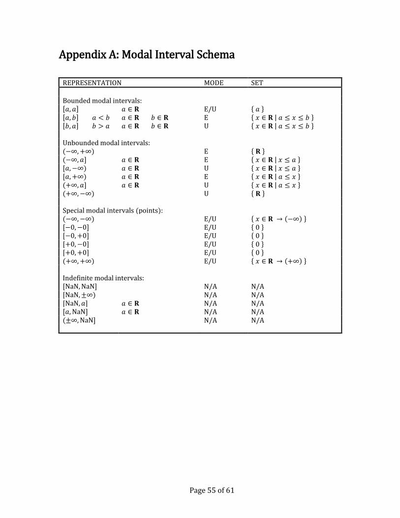
Page 55 of 61

Appendix A: Modal Interval Schema

REPRESENTATION MODE SET

Bounded modal intervals: 𝑎,𝑎 𝑎 ∈ 𝐑 E/U 𝑎 𝑎, 𝑏 𝑎 < 𝑏 𝑎 ∈ 𝐑 𝑏 ∈ 𝐑 E 𝑥 ∈ 𝐑 𝑎 ≤ 𝑥 ≤ 𝑏 𝑏,𝑎 𝑏 > 𝑎 𝑎 ∈ 𝐑 𝑏 ∈ 𝐑 U 𝑥 ∈ 𝐑 𝑎 ≤ 𝑥 ≤ 𝑏 Unbounded modal intervals: (−∞, +∞) E 𝐑 (−∞,𝑎] 𝑎 ∈ 𝐑 E 𝑥 ∈ 𝐑 𝑥 ≤ 𝑎 [𝑎,−∞) 𝑎 ∈ 𝐑 U 𝑥 ∈ 𝐑 𝑥 ≤ 𝑎 [𝑎, +∞) 𝑎 ∈ 𝐑 E 𝑥 ∈ 𝐑 𝑎 ≤ 𝑥 (+∞,𝑎] 𝑎 ∈ 𝐑 U 𝑥 ∈ 𝐑 𝑎 ≤ 𝑥 (+∞,−∞) U 𝐑 Special modal intervals (points): (−∞,−∞) E/U 𝑥 ∈ 𝐑 → −∞ [−0,−0] E/U 0 [−0, +0] E/U 0 [+0,−0] E/U 0 [+0, +0] E/U 0 (+∞, +∞) E/U 𝑥 ∈ 𝐑 → +∞ Indefinite modal intervals: [NaN, NaN] N/A N/A [NaN, ±∞) N/A N/A [NaN,𝑎] 𝑎 ∈ 𝐑 N/A N/A [𝑎, NaN] 𝑎 ∈ 𝐑 N/A N/A (±∞, NaN] N/A N/A

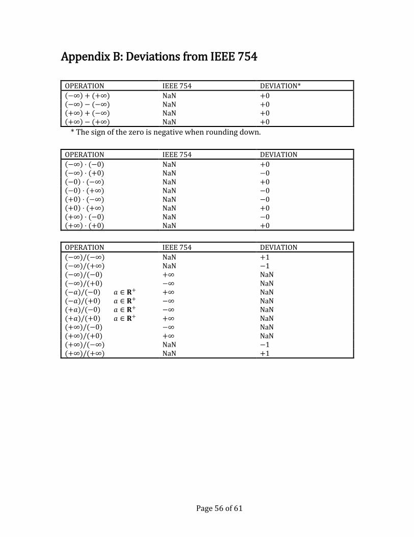
Page 56 of 61

Appendix B: Deviations from IEEE 754

OPERATION IEEE 754 DEVIATION*

−∞ + (+∞) NaN +0 −∞ − (−∞) NaN +0 +∞ + (−∞) NaN +0 +∞ − (+∞) NaN +0

* The sign of the zero is negative when rounding down.

OPERATION IEEE 754 DEVIATION

−∞ ⋅ (−0) NaN +0 −∞ ⋅ (+0) NaN −0 −0 ⋅ (−∞) NaN +0 −0 ⋅ (+∞) NaN −0 +0 ⋅ (−∞) NaN −0 +0 ⋅ (+∞) NaN +0 +∞ ⋅ (−0) NaN −0 +∞ ⋅ (+0) NaN +0

OPERATION IEEE 754 DEVIATION

(−∞)/(−∞) NaN +1 (−∞)/(+∞) NaN −1 (−∞)/(−0) +∞ NaN (−∞)/(+0) −∞ NaN (−𝑎)/(−0) 𝑎 ∈ 𝐑+ +∞ NaN (−𝑎)/(+0) 𝑎 ∈ 𝐑+ −∞ NaN (+𝑎)/(−0) 𝑎 ∈ 𝐑+ −∞ NaN (+𝑎)/(+0) 𝑎 ∈ 𝐑+ +∞ NaN (+∞)/(−0) −∞ NaN (+∞)/(+0) +∞ NaN (+∞)/(−∞) NaN −1 (+∞)/(+∞) NaN +1

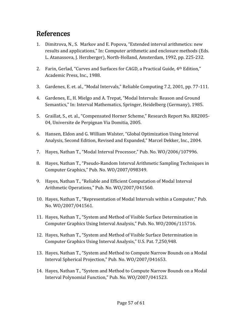
Page 57 of 61

References

1. Dimitrova, N., S. Markov and E. Popova, “Extended interval arithmetics: new

results and applications,” In: Computer arithmetic and enclosure methods Eds.

L. Atanassova, J. Herzberger), North-Holland, Amsterdam, 1992, pp. 225-232.

2. Farin, Gerlad, “Curves and Surfaces for CAGD, a Practical Guide, 4th Edition,”

Academic Press, Inc., 1988.

3. Gardenes, E. et. al., “Modal Intervals,” Reliable Computing 7.2, 2001, pp. 77-111.

4. Gardenes, E., H. Mielgo and A. Trepat, “Modal Intervals: Reason and Ground

Semantics,” In: Interval Mathematics, Springer, Heidelberg (Germany), 1985.

5. Graillat, S., et. al., “Compensated Horner Scheme,” Research Report No. RR2005-

04, Universite de Perpignan Via Domitia, 2005.

6. Hansen, Eldon and G. William Walster, “Global Optimization Using Interval

Analysis, Second Edition, Revised and Expanded,” Marcel Dekker, Inc., 2004.

7. Hayes, Nathan T., “Modal Interval Processor,” Pub. No. WO/2006/107996.

8. Hayes, Nathan T., “Pseudo-Random Interval Arithmetic Sampling Techniques in

Computer Graphics,” Pub. No. WO/2007/098349.

9. Hayes, Nathan T., “Reliable and Efficient Computation of Modal Interval

Arithmetic Operations,” Pub. No. WO/2007/041560.

10. Hayes, Nathan T., “Representation of Modal Intervals within a Computer,” Pub.

No. WO/2007/041561.

11. Hayes, Nathan T., “System and Method of Visible Surface Determination in

Computer Graphics Using Interval Analysis,” Pub. No. WO/2006/115716.

12. Hayes, Nathan T., “System and Method of Visible Surface Determination in

Computer Graphics Using Interval Analysis,” U.S. Pat. 7,250,948.

13. Hayes, Nathan T., “System and Method to Compute Narrow Bounds on a Modal

Interval Spherical Projection,” Pub. No. WO/2007/041653.

14. Hayes, Nathan T., “System and Method to Compute Narrow Bounds on a Modal

Interval Polynomial Function,” Pub. No. WO/2007/041523.

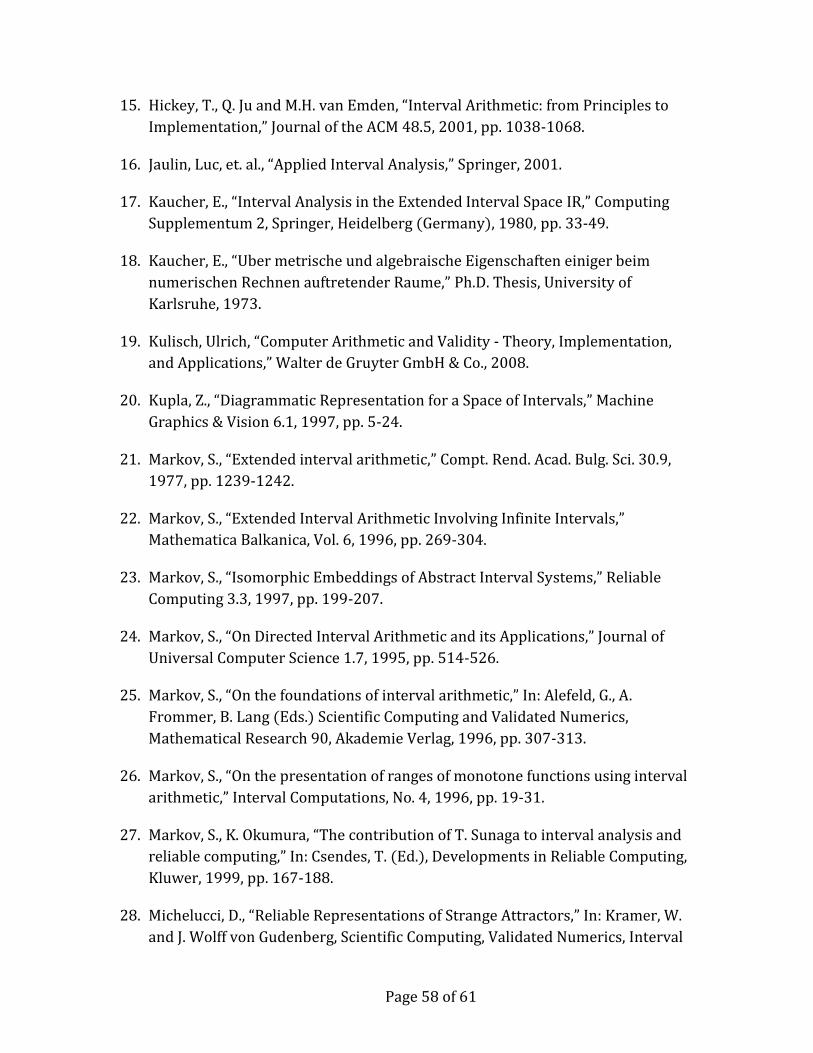
Page 58 of 61

15. Hickey, T., Q. Ju and M.H. van Emden, “Interval Arithmetic: from Principles to

Implementation,” Journal of the ACM 48.5, 2001, pp. 1038-1068.

16. Jaulin, Luc, et. al., “Applied Interval Analysis,” Springer, 2001.

17. Kaucher, E., “Interval Analysis in the Extended Interval Space IR,” Computing

Supplementum 2, Springer, Heidelberg (Germany), 1980, pp. 33-49.

18. Kaucher, E., “Uber metrische und algebraische Eigenschaften einiger beim

numerischen Rechnen auftretender Raume,” Ph.D. Thesis, University of

Karlsruhe, 1973.

19. Kulisch, Ulrich, “Computer Arithmetic and Validity - Theory, Implementation,

and Applications,” Walter de Gruyter GmbH & Co., 2008.

20. Kupla, Z., “Diagrammatic Representation for a Space of Intervals,” Machine

Graphics & Vision 6.1, 1997, pp. 5-24.

21. Markov, S., “Extended interval arithmetic,” Compt. Rend. Acad. Bulg. Sci. 30.9,

1977, pp. 1239-1242.

22. Markov, S., “Extended Interval Arithmetic Involving Infinite Intervals,”

Mathematica Balkanica, Vol. 6, 1996, pp. 269-304.

23. Markov, S., “Isomorphic Embeddings of Abstract Interval Systems,” Reliable

Computing 3.3, 1997, pp. 199-207.

24. Markov, S., “On Directed Interval Arithmetic and its Applications,” Journal of

Universal Computer Science 1.7, 1995, pp. 514-526.

25. Markov, S., “On the foundations of interval arithmetic,” In: Alefeld, G., A.

Frommer, B. Lang (Eds.) Scientific Computing and Validated Numerics,

Mathematical Research 90, Akademie Verlag, 1996, pp. 307-313.

26. Markov, S., “On the presentation of ranges of monotone functions using interval

arithmetic,” Interval Computations, No. 4, 1996, pp. 19-31.

27. Markov, S., K. Okumura, “The contribution of T. Sunaga to interval analysis and

reliable computing,” In: Csendes, T. Ed. , Developments in Reliable Computing,

Kluwer, 1999, pp. 167-188.

28. Michelucci, D., “Reliable Representations of Strange Attractors,” In: Kramer, W.

and J. Wolff von Gudenberg, Scientific Computing, Validated Numerics, Interval

Page 59 of 61

Methods, Kluwer, 2001, pp. 379-390.

29. Moore, R., “Interval Analysis,” Prentice Hall, N. J., 1966.

30. Moore, R., “Interval Arithmetic and Automatic Error Analysis in Digital

Computing,” Applied Math. & Stat. Lab., Stanford University Technical Report

No. 25, 1962; also: Ph.D. Dissertation, Stanford University, October 1962.

31. Neumaier, A., “Computer graphics, linear interpolation, and nonstandard

intervals,” http://www.mat.univie.ac.at/~neum/ms/nonstandard.pdf,

December 22, 2008.

32. Neumaier, A., “Grand Challenges and Scientific Standards in Interval Analysis,”

Reliable Computing 8.4, 2002, pp. 313-320.

33. Neumaier, A., “Vienna proposal for interval standardization,”

http://www.mat.univie.ac.at/~neum/ms/1788.pdf, November 21, 2008.

34. Ortolf, H. J., “Eine Verallgemeinerung der Intervallarithmetik,” Berichte der Ges.

Math. Datenverarbeitung, Bonn 11, 1969, pp. 1–71.

35. Piegl, Les A. and W. Tiller, “The NURBS Book, Second Edition,” Springer, 1996.

36. Popova, E. and W. Kraemer, “Inner and Outer Bounds for Parametric Linear

Systems,” Journal of Computational and Applied Mathematics 199.2, 2007, 310-

316.

37. Popova, E. D. and C. P. Ullrich, “Directed Interval Arithmetic in Mathematica:

Implementation and Applications”, Technical Report 96-3, Universitaet Basel,

January 1996.

38. Popova, E. D. and C. P. Ullrich, “Simplification of Symbolic-Numerical Interval

Expressions,” Proceedings of the 1998 International Symposium on Symbolic

and Algebraic Computations, ACM Press, 1998, pp. 207-214.

39. Popova, E. D. and C. Ullrich, “Generalising BIAS Specification,” Journal of

Universal Computer Science 3.1, 1997, pp. 23-41.

40. Popova, E. D., “Extended Interval Arithmetic in IEEE Floating-Point

Environment,” Interval Computations, No. 4, 1994, pp. 100-129.

41. Popova, E. D., “Interval Operations Involving NaNs,” Reliable Computing 2.2,

1996, pp. 161-165.

Page 60 of 61

42. Popova, E. D., “Multiplication Distributivity of Proper and Improper Intervals,”

Reliable Computing 7.2, 2001, pp. 129-140.

43. Popova, E. D., “On the Efficiency of Interval Multiplication Algorithms,”

Proceedings of III-rd International Conference “Real Numbers and Computers,”

Paris, April 27-29, 1998, pp. 117-132.

44. Sainz, M., E. Gardenes and L. Jorba, “Formal Solution to Systems of Interval

Linear or Non-Linear Equations,” Reliable Computing 8.3, 2002, pp. 189-211.

45. Sainz, M., E. Gardenes and L. Jorba, “Interval Estimations of Solution Sets to

Real-Valued Systems of Linear or Non-Linear Equations,” Reliable Computing

8.4, 2002, pp. 283-305.

46. Sederberg, T. W. and Farouki, “Approximation by Interval Bezier Curves,” IEEE

Computer Graphics and Applications 12.5, 1992, pp. 87-95.

47. Shary, Sergey P., “A New Technique in Systems Analysis under Interval

Uncertainty and Ambiguity,” Reliable Computing 8.5, 2002, pp. 321-418.

48. SIGLA/X Group Calm R., Estela M.R., et. al. , “Ground Construction of Modal

Intervals,” Proc. of MISC’99, University of Girona, Spain.

49. SIGLA/X Group Calm R., Estela M.R., et. al. , “Interpretability and Optimality of

Rational Functions,” Proc. of MISC’99, University of Girona, Spain.

50. SIGLA/X Group (Calm R., Estela M.R., et. al. , “Semantic and Rational Extensions

of Real Continuous Functions,” Proc. of MISC’99, University of Girona, Spain.

51. Snyder, John M., “Generative Modeling for Computer Graphics and CAD,

Symbolic Shape Design Using Interval Analysis,” Academic Press, Inc., 1992.

52. Stahl, Volker, “Interval Methods for Bounding the Range of Polynomials and

Solving Systems of Nonlinear Equations,” Johannes Kepler University, Austria,

1995.

53. Steele, Jr., Guy L., “Floating Point System With Improved Support of Interval

Arithmetic,” U.S. Pat. 7,069,288.

54. Stolfi, Jorge and L. H. de Figueirdedo, “Self-Validated Numerical Methods and

Applications,” Brazilian Mathematics Colloquium, IMPA, Rio de Janeiro, Brazil,

1997.

Page 61 of 61

55. Stolfi, Jorge, “Oriented Projective Geometry, A Framework for Geometric

Computations,” Academic Press, Inc., 1991.

56. Sunaga, T., “Theory of interval algebra and its application to numerical analysis,”

In: Research Association of Applied Geometry (RAAG) Memoirs, Vol. 2, 1958, pp.

29-46.

57. Walster, G. William, “Method and Apparatus for Representing Arithmetic

Intervals Within a Computer System,” U.S. Pat. 6,658,443.

58. Warmus, M., “Approximations and Inequalities in the Calculus of

Approximations. Classification of Approximate Numbers,” Bull. Acad. Polon. Sci.

Ser. Math. Astr. Phys., Vol. IX, No. 4, 1961, pp. 241–245.

59. Warmus, M., “Calculus of Approximations,” Bull. Acad. Polon. Sci., Cl. III, Vol. IV,

No. 5, 1956, pp. 253–259.