CONCEPT OF MODEL BASED TAMPERING FOR ...ise.tamu.edu/People/faculty/Bukkapatnam/PDFs/14journal...7 and Satish T.S. Bukkapatnam, Assistant Professor of Industrial 8 and Systems Engineering2

1

2 CONCEPT OF MODEL BASED TAMPERING FOR3 IMPROVING PROCESS PERFORMANCE:4 AN ILLUSTRATIVE APPLICATION TO5 TURNING PROCESS

6 Raj Palanna, Manufacturing and Quality Engineering Manager,1,*

7 and Satish T.S. Bukkapatnam, Assistant Professor of Industrial8 and Systems Engineering2

9 1Honeywell Aerospace, Torrance, CA, USA

10 2University of Southern California, Los Angeles, CA, USA1112

13 ABSTRACT

14 This paper presents the concept of a methodology called Model Based

15 Tampering (MBT), that considers the non-linear and stochastic nature of

16 process dynamics, to compensate, in real-time, the effects of process

17 degradation on the performance. The uniqueness of this concept emerges

18 from the ability to combine and utilize the structures of the existing

19 models to fit tractable and robust real-time control models in the form of

20 low-dimensional nonlinear stochastic differential equations (n-SDEs). As

21 an illustrative application of MBT, the minimization of diameter variation

22 due to tool degradation in the turning process is considered. Through a

23 series of simulation runs, the use of MBT was found to reduce diameter

24 variation by 97%. The methodology is applicable to a wide range of man-

25 ufacturing processes.

*Corresponding author. E-mails: [email protected], [email protected]

AQ2 AQ3

AQ4

AQ5

AQ1

263

Copyright D 2002 by Marcel Dekker, Inc. www.dekker.com

MACHINING SCIENCE AND TECHNOLOGY, 6(2), 263–282 (2002)

120013166_MST_6_2_R1_SPI

F1

F2

30 INTRODUCTION

31 Design tolerances have shrunk significantly during the past 60 years (see

32 Figure 1) as industries strive to achieve increasingly higher levels of product quality.[1]

33 In the 1940s and 50s, dimensional tolerances on prints were usually specified in

34 thousandths of an inch. Later, they shrank to ten-thousandths. Today, millionths of an

35 inch are not uncommon.[2] However, despite all the tightening of tolerances, machine

36 tools have not changed drastically over the years. Therefore, effective control systems

37 such as model based tampering (MBT), which is conceptualized in this paper, will

38 become necessary in order to meet the growing performance requirements without

39 altering the machine tool configurations.

40 A schematic of the MBT concept is given in Figure 2. Here, performance refers

41 to the system outputs of interest. The various state variables define the state of the

42 system at any point in time. The input is the external tamper that is provided based on

43 the system outputs. As shown in the topmost plot of the figure, the variability

44 associated with the performance as a result of process degradation can be significantly

45 reduced through the use of appropriately synthesized tamper input. Thus, MBT will

46 help us improve the performance of a manufacturing system without changing any

47 fundamental system components.[3] All one needs is an intelligent controller to com-

48 pensate for the effects of process degradation. Many difficult processes can benefit

49 tremendously from the use of this technique.[4]

50 The quality and six sigma schools of thought show the benefits of not tampering

51 for noise, but compensating for signal shifts.[1] However, these concepts and the body

52 of knowledge are predominantly limited only to linear systems.

53 Machining dynamics is non-linear and the noise contamination makes the dyna-

54 mics complex from a modeling and control standpoint.[5] Hence, non-linear stochastic

55 differential equations (n-SDEs) are the natural means to model these processes.

56 However, earlier efforts did not consider n-SDEs for modeling the dynamics of pro-

57 cess degradation, as well as the effects of degradation on the process performance

58 or quality.

59 Previous works on adaptive statistical process control predominantly used

60 algebraic models,[6–9] and process dynamics, especially the underlying nonlinearities

0.051

0.025

0.013

0.0050.003 0.0010.000

0.010

0.020

0.030

0.040

0.050

0.060

1940 1950 1960 1970 1980 1990 2000

Year

mm

?

Figure 1. Shrinking of ‘‘usual’’ tolerance specifications during the last 60 years.[1]

264 PALANNA AND BUKKAPATNAM

120013166_MST_6_2_R1_SPI

61 and stochasticity, was not thoroughly considered. Models employed for geometric

62 adaptive control (GAC) did not consider non-linear dynamics of degradation processes.

63 In addition, the noise associated with degradation processes was not modeled in the

64 GAC-related efforts.[10–13] The past research efforts concentrated on compensating for

65 ‘‘mean’’ degradation without a thorough characterization of the noise and nonlinearities

66 associated with the system. The lack of adequate theoretical foundations and

67 computational infrastructure to analyze and model n-SDEs has previously been the

68 main barrier to their widespread application to engineering domains. Because of these

69 difficulties, in current machining practice, a tamper is seldom used to compensate for

70 the effects of degradation. Thus, the use of n-SDEs to model process dynamics,

71 degradation processes, input-state-output relationships, and thence synthesize control

72 inputs makes MBT unique.

73 In this paper the basic concept of MBT as well as the major stages of the

74 methodology (see APPROACH) is presented. The key to MBT is a new method

75 for modeling process dynamics and degradation using n-SDEs, wherefrom appro-

76 priate tamper inputs can be synthesized and enforced in real-time. The experimental

77 proof-of-concept validation of this new modeling scheme is described in PROOF-

78 OF-CONCEPT VALIDATION OF N-SIDE MODELING SCHEME. In AN ILLUS-

Figure 2. A schematic of dynamic trends of different variables in a system.

CONCEPT OF MODEL BASED TAMPERING 265

120013166_MST_6_2_R1_SPI

79 TRATIVE APPLICATION OF MBT TO LATHE OPERATIONS, presents an initial

80 illustrative application of MBT to the turning process.1 The application domain was

81 chosen thus because a fair amount of research progress has already been made in

82 modeling tool degradation and process dynamics in machining.[14–17] The simulation

83 studies involving this illustrative example indicate the potential of MBT in con-

84 trolling the effects of process degradation on product quality.

85 APPROACH

86 The nomenclature employed in this paper is summarized in Figure 3. Process

87 dynamics, quantified by a state variable x—an n dimensional vector—degrades over

88 time t. This degradation of process states progressively lowers the overall performance

89 quality, represented by a performance variable (vector) z. For example, in the case of

90 lathe turning process, appropriate quantifiers of diameter and surface finish comprise

91 the output performance variable z while x may be composed of those representing tool

92 wear, forces, vibrations, etc. Performance variables are assumed to be among the

93 measured process outputs vector y. Signals from force, vibration and temperature

94 sensors may constitute y. The state of the process is estimated (the estimates are

F3

),,( puxZz =

uxYxGxFx )()()( ++= ω

)(XHy =

uYGxFx )()(ˆ)(ˆˆ •+•+= ω

),ˆ( pxUu =

u

y

u

x

x̂

z

),,( puxHy =

Figure 3. Systems perspective of the application of MBT.

1The authors note that the experimentation and models involved in the proof-of-concept validation

of the modeling scheme are different from and unrelated to those employed in the simulation

studies used to illustrate the overall MBT. While the experimentation domain was chosen to

facilitate a basic proof-of-concept validation of the modeling scheme, the simulation domain was

selected to enable a simple illustration of the MBT concept.


120013166_MST_6_2_R1_SPI

95 represented by x̂) from measurements of process outputs y, and a tamper (control input)

96 u is introduced into the process in order to meet the overall performance objectives.

97 p represents the process parameters of the machine. Here, F, G, H, Y, U, Z are

98 appropriate transformations.

99 The MBT methodology, summarized in Figure 4, essentially consists of quan-

100 titatively characterizing the degradation of a process (as quantified from the dynamics

101 of state variables), in real-time, from on-line sensor signals; and compensating the

102 effects of degradation on performance by continuously using ‘‘a knob(s)’’ which is one

103 of the control inputs u. The tamper (i.e., the control input u) for the system output has

104 to be synthesized based on the dynamics of the system and not by monitoring the

105 performance variables alone. For a given manufacturing process scenario, the variables

106 x, y, z, etc. may be determined using Process Failure Modes and Effects Analysis and

107 other screening techniques.[1] Here, y is a function of system state variables x, and its

108 dynamics is governed by

y ¼ Hðx; u; pÞ; ð1Þ

109110 where H(.) can be a differentio-integral transformation. The system state vector x is

111 governed by an n-SDE of the form

dx=dt ¼ FðxÞ þ GðxÞoþ YðxÞu; ð2Þ

112113 where F(x) is a vector field denoting the deterministic portion of the dynamics of

114 x, G(x)o represents multiplicative dynamic noise, and Y(x) u represents the control

115 input. Understanding and modeling of the underlying relations allows to ‘‘adjust’’ u in

116 such a way that the performance variable would remain stationary.

117 Thus, the MBT methodology critically hinges on the modeling scheme to derive

118 control models for the non-linear stochastic processes. The overall modeling scheme

Process Characterization andData CollectionStage I

Modeling(To Quantatively Represent

Process Dynamics)

Tamper Strategy andTamper Refinement

Validation

Stage II

Stage III

Stage IV

Figure 4. Generic MBT flow chart.

F4


120013166_MST_6_2_R1_SPI

119 consists of deriving the structure of the model and fitting the selected structure using

120 actual process outputs.

121

122 Structure Selection

123 The available analytical models serve as excellent starting points for deriving

124 appropriate model structures of the form (1) and (2). For example, structure of Koren

125 and Lenz’s model[16] is adequate for capturing tool wear dynamics. When adequate

126 structures are not available or if the structures are intractable for model fitting, one may

127 extract simpler model structures with polynomial non-linearity by studying the un-

128 derlying non-linear behaviors.[21] For example, near the range of parameters and

129 initial conditions at which dynamics undergoes a Hopf bifurcation (a type of sudden

130 qualitative change in the behavior of the process), models with quadratic or cubic

131 non-linearity will usually suffice.[18]

132

133 Model Fitting

134 Direct fitting of an n-SDE from the measured signals is extremely cumbersome.

135 Therefore the following Fokker–Planck equation is set up for the probability density

136 p(x, t) of the state variables x:[19]

@

@tpðx; tÞ ¼

Xn

i¼1

@

@xi

�D

ð1Þi ðx; tÞpðx; tÞ

�þ 1

2

Xn

ij¼1

@2

@xi@xj

�D

ð2Þij ðx; tÞpðx; tÞ

�ð3Þ

137138

139 The coefficients Dj(1) are called drift coefficients, Dij

(2) are called diffusion

140 coefficients. These coefficients are specific functions of F and G as defined in [20], and

141 they can be determined from the conditional probabilities computed from realizations

142 of x, i.e., from the measured signals or transformations of these signals. This new

143 model fitting procedure is outlined in Appendix A.

144

145 PROOF-OF-CONCEPT VALIDATION OF n-SDE MODELING SCHEME

146 The feasibility of the n-SDE modeling scheme concisely presented in the

147 previous section has been validated through the second author’s earlier efforts to model

148 machining dynamics from accelerometer signals.[21] Due to its complicated nature and

149 the multifarious parametric relationships, machining dynamics was modeled in a

150 piecewise manner over the operating range of the process parameters. The dependence

151 of machining dynamics on only one process parameter, i.e., the depth of cut d, was

152 modeled from signals extracted from experiments.[21] All experiments were conducted

153 on a 12 HP Boehringer lathe. A large diameter SAE 6150 high alloy steel billet was

154 chosen as the workpiece material. A coated carbide tool of grade K420 with positive

155 rake angle and specification SPG-422 was used. Two PCB accelerometers, located on

156 the fixture near the tail-end of the tool-holder measured vibrations along the main and

157 feed directions. The vibration signals from the two accelerometers were passed through

158 two separate 480D06 type PCB charge amplifiers, and they were digitized using a 2630


120013166_MST_6_2_R1_SPI

F5

F6

159 Tektronix Fourier Analyzer. The sampling rate for digitization was chosen to be 20

160 kHz, based on the earlier observations of the signal characteristics. All measured

161 signals were 4096 data points long.

162 Since the occurrence of chatter was well spread out in the d-space, cutting speed

163 V = 82.6 m/min was used. Vibration signals were captured from d = 0.25 mm to

164 d = 11.43 mm. All components of the piecewise model had two degrees-of-freedom

165 (revealed from experimental characterization); hence a four-dimensional x was used

166 whose components, respectively, represent instantaneous tool deflection and velocity

167 along the main (tangential) and the feed direction.

168 The first step in the modeling scheme consisted of obtaining the bifurcation

169 diagram from measured signals. The bifurcation types delineated by the bifurcation

170 diagram determined the order of polynomial non-linear structure of the model. Next,

171 the novel fitting procedure, which can fit a more generic class of non-linear stochastic

172 models as described in the previous section was applied.

173 This new modeling scheme is illustrated with respect to accelerometer signals

174 measured along the feed direction. Figures 5 and 6 show the time and frequency

175 response plots2 of the signal. One may note that although the signal appears to be

176 periodic with a few and finite number of dominant frequencies, the underlying

177 dynamics has been shown to be nonlinear and chaotic.[21] Based on these plots and

2The plots are also called the frequency–magnitude plots. The power spectrum is a plot of the

magnitude-squares verses frequency.

Figure 5. Time portraits of the deflection and velocity of a cutting tool along the two orthogonal

directions.


120013166_MST_6_2_R1_SPI

178 Bukkapatnam’s earlier analysis of bifurcations in this process, an n-SDE model with at

179 most quadratic terms of the form will be adequate:[21]

d

dt

x1

x2

x3

x4

2666664

3777775¼

x2

�c1x2 � c2x1 þPMk¼3

ckXu1k

1 Xn1k

2 Xu2k

3 Xn2k

4

x4

�d1x4 � d2x3 þPMk¼3

dkXu1k

1 Xn1k

2 Xu2k

3 Xn2k

4

2666666664

3777777775

þ

0

�w1x2 � w2x1 þPQk¼3

wkXu1k

1 Xn1k

2 Xu2k

3 Xn2k

4

0

�x1x4 � x2x3 þPQk¼3

xkXu1k

1 Xn1k

2 Xu2k

3 Xn2k

4

2666666664

3777777775o ð4Þ

180181

Figure 6. Frequency response (magnitude) plots of the measured signals along the two orthogonal

directions.3

3The plots in Figures 6 and 7 are the default frequency response (magnitude) plots from Matlab, and

the frequency bins must be interpreted thus.


120013166_MST_6_2_R1_SPI

182 In the above equation, c2 and d2 represent the stiffness terms, c1 and d1 represent

183 the damping terms, ck and dk k > 2 are the coefficients of the nonlinear terms, and w’s

184 and x’s represent the coefficients (nonlinear) noise gain terms. Typical values of these

185 terms for a representative case were as follows: M = 2, Q = 0, c1 = 669, c2 = 4.5e7,

186 c3 = � 1.3e7 (coefficient of x3), c4 = 2e15 (coefficient of x12), d1 = 1162, c2 = 2.8e6,

187 d3 = 4e7 (coefficient of x1), d4 = 3.5e15 (coefficient of x32) w1 = 4.8, w2 = 4.1, x1 = 1.6,

188 x2 = 2.1, and all remaining coefficients were zero.

189 A comparison of the frequency response (magnitude) graphs of 15 Monte-Carlo

190 runs of solutions from the model with the frequency response (magnitude) graph of the

191 original signal is shown in Figure 7. A near-perfect alignment of the graphs in the

192 figure clearly indicates that the models fitted through this new scheme can correctly

193 capture the dominant frequency domain features. Further, for signals with high levels

194 of bursts such as acoustic emission, the multiplicative noise terms can replicate the

195 characteristic time-domain features more faithfully than most modeling schemes, which

196 are limited to fitting additive noise terms alone. These experimental studies have also

197 shown that the solutions of models fit from the new modeling scheme lie within 10%

198 of the original signal.

199

200 AN ILLUSTRATIVE APPLICATION OF MBT TO LATHE OPERATIONS

201 Simulation Model Development

202 The concept of MBT was studied and illustrated using simple simulations

203 conducted in the context of tool degradation in lathe turning operations. Extensive

204 literature review as well as practical process knowledge was used to develop a

F7

Figure 7. Plot comparing the frequency response of solutions from the model runs with that of the

original signal.


120013166_MST_6_2_R1_SPI

205 simulation model that adequately represents the machining phenomenon.4 Towards

206 building this simulation model, first the tool wear model presented by Danai and

207 Ulsoy[15] was adapted. The Danai–Ulsoy model combines the earlier Koren–Lenz[16]

208 model of force, diffusion flank wear, abrasive flank wear, and crater temperature, Usui

209 et al’s model[22] of crater wear dynamics, and Chao and Trigger’s flank temperature

210 model.[14] The Danai–Ulsoy model was converted into a truly non-linear state space

211 form as shown in Appendix B. Experimenting on model parameters the representation

212 was further fine-tuned. Subsequently noise terms were added to the model to capture

213 uncertainties in the actual tool degradation.5

214 The basic relationships in this simulation model are summarized using a bipartite

215 graph[23] shown in Figure 8. A bipartite graph representation delineates how different

216 performance, state and input variables relate to each other. Here, the performance

217 variable is the diameter variation. State variables are given by flank wear wf, crater

218 wear wc, force F, flank temperatures yf and crater temperature yc. The noise in the

219 models is represented by SE*’s. The numbers given in the square boxes correspond to

220 the equations given in Appendix B. Box 9 refers to the trivial equation the forms the

221 basis for computing the tamper input u.

222

223 Experimentation Strategy

224 Once the simulation model was developed, a very rigorous data generation,

225 analysis and validation procedure was conducted. Design of Experiment (DOE) body of

226 knowledge was systematically used to explore the performance envelope of MBT on

227 lathe operations as represented by this simulation model.[24] This helped to accurately

228 locate the optimum control strategy or process parameter settings for this illustrative

229 case of minimizing diameter variation.

230 Two sets of designed simulations were conducted. First, the model was explored

231 with no noise added. The basic assumption was that the process model completely

232 captures the overall process dynamics and other relationships. The purpose of this study

233 was to assess MBT under complete knowledge. The validation studies in this case was

234 done using a 28-3ResIV fractional factorial DOE with one center point and design

235 generators: F = ABC, G = ABD and H = BCDE.[24] This was followed by an opti-

4At this stage, the authors wish to emphasize that ‘‘model’’ in MBT refers to a control model that

is developed from actual process observations, as opposed to a simulation model, which has been

used to validate MBT.5This illustrative example is unrelated to the experimentation presented in PROOF-OF-

CONCEPT VALIDATION OF n-SDE MODELING SCHEME to validate the modeling scheme.

Further, the model structures presented in Appendix B for the simulation model are unrelated to

the structures presented in PROOF-OF-CONCEPT VALIDATION OF n-SDE MODELING

SCHEME (i.e., Eq. 4). The simulation model was chosen to be different from the experimentation

because the objective for AN ILLUSTATIVE APPLICATION OF MBT TO LATHE OPERA-

TIONS is to present a simple illustration of the overall concept, while the objective of PROOF-

OF-CONCEPT VALIDATION OF n-SDE MODELING SCHEME is to provide a convincing

proof-of-concept for the new n-SDE modeling scheme, which forms the most critical part of the

overall MBT methodology.

F8


120013166_MST_6_2_R1_SPI

236 mization run over 2 factors. There were 33 total runs for this experiment. The DOE

237 responses for the conducted study are as follows. Standard deviation sD measures the

238 total variation in the output, i.e, the diameter, and Diameter sigma sD100 measures

239 output variation after 100 sec after the application of the tamper. Tool wear Wf is the

240 total flank tool wear after 1000 sec. Wf is the sum of Wf1 and Wf2, which are flank

241 wear due to abrasion and diffusion, respectively, after 1000 sec. Tool Wear Wc is the

242 total crater tool wear after 1000 sec. Tamper Energy is the response that measures total

243 tamper energy consumed after 1000 sec. The eight design factors were as follows:

244 . Cutting Speed (mm/sec)

245 . Feed (mm/rev)

246 . Depth of Cut (mm)

247 . Rake angle (deg)

248 . Clearance angle (deg)

249 . Tamper smoothness, a 0,1 variable depending whether the tamper inputs were

250 smoothed

251 . Tamper rate, the maximum allowable variation of tamper inputs in a unit time

252 (mm/sec)

253 . DeltaT, the inter-tamper time (sec)

1

2 4

F

Z

Wf

Wc

t

thetaC

5

6

3

Wf2 Wf1

8

thetaf

7

Bipartite Graph - Model Structures for Diameter Machining

- Variable - Relationship

Noise

SEcNoise

SEd

Noise

SEd

U

9

Tamper

Figure 8. Bipartite graphs capturing the relationships in the simulation model.


120013166_MST_6_2_R1_SPI

254 This experiment provided a baseline indication of how the simulation models

255 would behave for different tamper inputs under different conditions with noise

256 introduced into the models.

257 Next, noise was considered in the simulation model, and it was assumed that the

258 control model captures only the deterministic portion and the overall noise structure.

Noise on w f1 Noise on Wf2 Noise on Wc Tamper smoot Tamper Rate Rake Angle DeltaT

0.00

001

0.00

002

0.00

003

0.00

001

0.00

002

0.00

003

0.00

001

0.00

002

0.00

003 No

Yes

0.00

01

0.00

05

0.00

10 0 5 10 2 60.00017

0.00027

0.00037

0.00047

0.00057

Avg

Dia

Sig

mMain Effects Plot - Data Means for Avg Dia Sigm

Figure 9. A representative DOE main effects plot.

0.00

001

0.00

003

0.00

001

0.00

003

No Yes

0.00

01

0.00

10

0 10 2 10

0.00020

0.00045

0.00070

0.00020

0.00045

0.000700.00020

0.00045

0.000700.00020

0.00045

0.000700.00020

0.00045

0.000700.00020

0.00045

0.00070Noise on wf1

Noise on Wf2

Noise on Wc

Tamper smoot

Tamper Rate

Rake Angle

DeltaT

0.00001

0.00003

0.00001

0.00003

0.00001

0.00003

No

Yes

0.0001

0.0010

0

10

Interaction Plot - Data Means for Avg Dia Sigm

Figure 10. A representative DOE interaction plot.


120013166_MST_6_2_R1_SPI

259 The purpose of this study was to gage MBT under incomplete knowledge of process

260 dynamics. The overall process dynamics equations are summarized in Appendix B. The

261 second DOE was a 27-2ResIV fractional factorial design. Each treatment had three

262 replicates with 33 different treatments.

263 . Noise level on Wf1, measured in terms of the noise gain term (mm)

264 . Noise level on Wf2, measured in terms of the noise gain term (mm)

265 . Noise level on Wc, measured in terms of the noise gain term (mm)

266 . Tamper smoothness

267 . Tamper rate

268 . Rake angle

269 . DeltaT, the inter-tamper time (sec)

270 These simulations gave an understanding of the performance of the system under

271 noise conditions and helped validate MBT in a more representative real machining

272 environment.

273 There were three output parameters of interest in this second study: Diameter

274 variation after tamper, Tamper energy used, Overall diameter variation, listed in order

275 of importance. Also, data was collected on two other parameters of interest, i.e., Wf

276 and Wc, in order to monitor the system and understand its states. All the experiments

277 were run for a time period of 1000 sec with data being collected at 0.5 sec intervals.

278 Figure 9 shows a typical main effects plot used in the analysis and Figure 10 shows a

279 typical interactions plot used in the analysis. Statistical validation techniques like

280 normal probability plots (a typical example shown in Figure 11) and Pareto of effects

281 were used. The plots of residuals vs. order of model terms, residuals vs. fitted value,

0 10 20 30

-2

-1

0

1

2

Standardized Effect

Nor

mal

Sco

re

E

DDE

CG

CDECD

DF

G

Normal Probability Plot of the Standardized Effects(response is Tamper E, Alpha = .10)

A: Noise onB: Noise onC: Noise onD: Tamper sE: Tamper RF: Rake AngG: DeltaT

Figure 11. A representative normal probability plot. Here the letters A through G, respectively,

represent the seven design factors used in the simulations.

F11

F9

F10


120013166_MST_6_2_R1_SPI

282 a normal probability plot of residuals and a histogram of residuals revealed the

283 characteristics of the randomness underlying the outputs and the residuals of the model

284 under various conditions.

285 The experiments helped set the optimum settings for the lathe model. Figure 12

286 shows a typical graph of diameter vs. time without MBT. The following were found

287 from the simulations to be the optimum settings for process parameters and control

288 inputs under MBT:

289 . Maintain Rake Angle at 100

290 . Keep Tamper rate High

291 . Use Tamper interval = 2 sec

Time

mm

Figure 13. Typical output with MBT.

Time

mm

Figure 12.

F12

AQ6

/AQ6


120013166_MST_6_2_R1_SPI

292 The plot in Figure 13 gives a typical example of system output performance with

293 MBT employed. From the plots it is evident that the diameter variation is lower by

294 97% compared to variation without MBT. This lower variation of diameter can help

295 produce consistently high quality products that provide more value to the customer.

296

297 SUMMARY AND FUTURE RESEARCH

298 The key idea in MBT is to use the superior n-SDE models to compensate for the

299 effects of process degradations. The tamper inputs generated based on these n-SDE

300 models are, in principle, superior to those generated through alternative methods such

301 as stochastic adaptive control (SAC), especially to nonlinear manufacturing processes

302 such as turning. This is because models for SAC have predominantly neglected the

303 nonlinear and chaotic dynamics of the underlying process, and they may not be ade-

304 quate in the presence of bifurcations.

305 Effectiveness of MBT was tested under various levels of system noise. MBT was

306 very successful in reducing variation at lower levels of noise. However, after the noise

307 levels reached a certain threshold magnitude, MBT did not yield any benefit in terms

308 of variation reduction. The major reason for this trend is that under higher noise levels

309 the model accuracies tend to be significantly low. As a result, tamper inputs generated

310 using the model can not adequately compensate for the effects of degradation.

311 This effort has been successful in proving the feasibility of the concept of MBT

312 using a simple case of controlling diameter by appropriately compensating for tool

313 degradation. The ongoing research at USC builds this concept along two main fronts:

314 The first involves adapting MBT to control the surface finish while grinding shafts of a

315 critical aircraft component produced at Honeywell Aerospace, California. The second

316 involves refining the modeling scheme by conducting further rigorous experimentation

317 and analysis, which lead to a robust multi-application MBT methodology.318

319 ACKNOWLEDGMENTS

320 The authors thank the anonymous reviewers for their constructive comments that

321 have helped improve this manuscript. Bukkapatnam acknowledges National Instru-

322 ments as well as Powell Foundation Fellowship for supporting the reported research.

323 APPENDIX A

324 The relations between the sets of coefficients of Eq. 2 and the Fokker–Planck

325 Eq. 3 under Stratonovich definitions are given by [20]:

Dð1Þi ðxÞ ¼ lim

Dt!0

1

DtE½xiðt þ DtÞ � xiðtÞ� i ¼ 1; 2; . . .

Dð2Þij ðxÞ ¼ lim

Dt!0

1

DtE½ðxiðt þ DtÞ � xiðtÞÞðxjðt þ DtÞ � xjðtÞÞ�

i ¼ 1; 2; . . . n j ¼ 1; 2; . . . n ðA1-1Þ326327

F13


120013166_MST_6_2_R1_SPI

328 where

hoðtÞi ¼ E½oðtÞ� ¼ 0

hoðt1Þoðt2Þi ¼ Eðoðt1Þoðt2ÞÞ ¼ Q:dðt1; t2Þ ðA1-2Þ

329330

331 For the considered class of stationary continuous Markovian process with white

332 dynamic noise, where the validity of the Markovian property may have been achieved

333 by introducing delay coordinates, it is always possible to determine drift and diffusion

334 terms directly from measured outputs by using the Eqs. 3 and 4.

335 As long as one is looking at observed steady state signals, which emanate from

336 the vicinity of an attractor, the following relationship holds:

pðxðtÞÞ ¼ pðxðsÞÞ 8t; s ðA1-3Þ

337338 and only the conditionals vary. Therefore one long signal (time series) is adequate.

339 Furthermore, Dj(1) and Dij

(2) they have no explicit time dependence. The needed

340 conditional probability density distribution can be determined numerically from the

341 data set by calculating histograms. When signals do not emanate from the vicinity

342 of an attractor, one needs ensembles of the solutions to (2), with all solutions

343 emerging from same initial conditions. Also, if one assumes a polynomial structure

344 for F and a constant g, one can tractably fit the structures according to (4) using

345 multiple regression or generalized regression.[21] Here the residues of regression fit

346 will yield g.

347

348 APPENDIX B

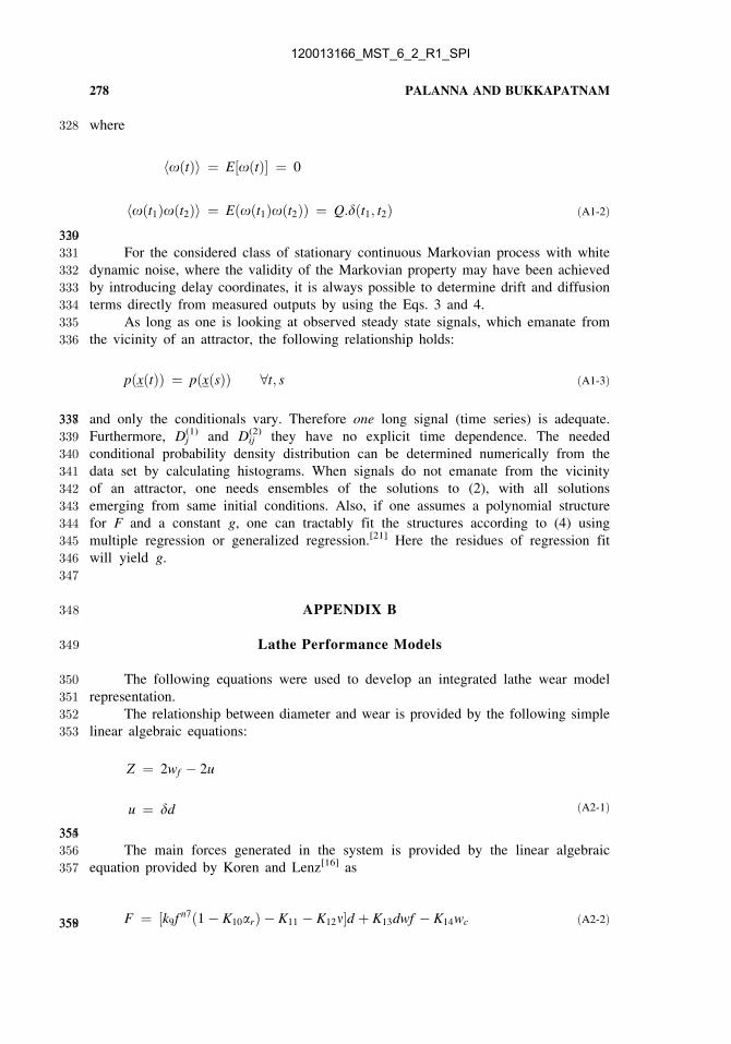
349 Lathe Performance Models

350 The following equations were used to develop an integrated lathe wear model

351 representation.

352 The relationship between diameter and wear is provided by the following simple

353 linear algebraic equations:

Z ¼ 2wf � 2u

u ¼ dd ðA2-1Þ

354355

356 The main forces generated in the system is provided by the linear algebraic

357 equation provided by Koren and Lenz[16] as

F ¼ ½k9f n7ð1 � K10arÞ � K11 � K12n�d þ K13dwf � K14wc ðA2-2Þ358359


120013166_MST_6_2_R1_SPI

360 The total f flank wear is given by a linear additive equation

wf ¼ wf 1 þ wf 2 ðA2-3*Þ361362

363 Crater wear is represented using a non linear differential equation given by Usui

364 et al.[22] as

�wc ¼ K4Fn exp½�K5=ð273 þ ycÞ� ðA2-4*Þ

365366

367 The crater temperature, which is needed for the crater wear equation, is provided

368 by a linear algebraic model of Koren and Lenz[16] as

yc ¼ K8Fnn4f n5dn6 ðA2-5Þ

369370

371 The abrasive flank wear dynamics is taken from [16] and it is given by a linear

372 differential equation

ðl0=nÞ �wf 1 þ wf 1 ¼ K1 cos arF=ð fdÞ ðA2-6Þ373374

375 The flank wear diffusion dynamics is obtained from [16] and it is given by a

376 nonlinear differential equation

�wf 2 ¼ K2

ffiffiffin

pexp½�K3=ð273=yf Þ� ðA2-7Þ

377378

379 Chao and Trigger[14] provided the following equation governing the flank

380 temperature, whose values are needed for the solution of flank wear diffusion equation

yf ¼ K6nn1f n2 þ K7wn3f ðA2-8Þ

381382

383 The table of constants for the models is provided in Appendix C.384385

386 Lathe Performance Models with Noise

387 The relationships of the two types of flank wear was modified as follows:

wf ¼ wf 1 þ wf 2 þ 0:00001o ðA2-3Þ388389

390 Crater wear equation was modified as

�wc ¼ K4Fn exp½�K5=ð273 þ ycÞ� þ 0:00001o ðA2-4Þ

391392

393 Referring back Figure 2, Eqs. A2-3,4,6,7) govern the dynamics of the state x, and

394 (A2-2,3,5,8) determine the process outputs y.


120013166_MST_6_2_R1_SPI

AP

PE

ND

IXC

Ta

ble

1.

Mo

del

Par

amet

ers

Use

din

the

Sim

ula

tio

no

fth

eN

on

lin

ear

Mo

del

Ty

pic

alW

ork

pie

ceC

utt

ing

Co

nd

itio

ns

Par

amet

erV

alu

esV

alu

eU

sed

Mat

eria

lT

oo

lM

ater

ial

v(m

/min

)f

(mm

/rev

)d

(mm

)R

ef.

K1

5.2

E-5

5.2

E-5

Ste

elC

arb

ide

18

00

.28

52

.5K

ore

nan

dL

enz,

19

70

K2

10

–2

01

5A

lSl

10

50

Ste

elP

10

Car

bid

e–

––

Ko

ren

and

Len

z,1

97

0

K3

10

,00

01

0,0

00

AlS

l1

05

0S

teel

P1

0C

arb

ide

––

–K

ore

nan

dL

enz,

19

70

K4

–8

0.2

5%

cst

eel

P2

0C

arb

ide

10

0–

35

00

.22

Tak

ahas

hi

etal

.,1

97

2

K5

22

,00

02

2,0

00

0.1

5–

0.4

5%

cst

eel

P2

0C

arb

ide

25

0–

35

00

.2,

0.2

62

Tak

ahas

hi

etal

.,1

97

2

K6

–7

24

14

2st

eel

Car

bid

e9

0–

21

00

.17

–0

.28

2.5

Ch

aoan

dT

rig

ger

,1

95

8

K7

–2

50

04

14

2st

eel

Car

bid

e9

0–

21

00

.17

–0

.28

2.5

Ch

aoan

dT

rig

ger

,1

95

8

K8

0.0

5–

0.0

60

.05

6S

teel

Car

bid

e–

––

Ko

ren

and

Len

z,1

97

0

K9

16

30

–1

96

01

96

02

Kh

1st

eel

20

A0

Car

bid

e1

10

0.1

–0

.84

Ko

ren

and

Len

z,1

97

0

K1

00

.51

–0

.63

0.5

7S

teel

Car

bid

e–

––

Ko

ren

and

Len

z,1

97

0

K1

10

.05

K5

86

Ste

elC

arb

ide

––

–K

ore

nan

dL

enz,

19

70

K1

20

.10

.1S

teel

Car

bid

e3

60

––

Ko

ren

and

Len

z,1

97

0

K1

33

00

–6

00

50

00

.45

%C

stee

lP

20

Car

bid

e–

0.2

–K

ore

nan

dL

enz,

19

70

K1

42

00

02

00

03

8N

CD

4S

teel

H.S

.S.

50

0.1

22

.5M

ich

elet

tiet

al.,

19

67

I 03

00

–7

00

50

0S

teel

Car

bid

e–

––

Ko

ren

and

Len

z,1

97

0

n1

–0

.44

14

2st

eel

Car

bid

e9

0–

21

00

.17

–0

.28

2.5

Ch

aoan

dT

rig

ger

,1

95

8

n2

–0

.64

14

2st

eel

Car

bid

e9

0–

21

00

.17

–0

.28

2.5

Ch

aoan

dT

rig

ger

,1

95

8

n3

–1

.45

41

42

stee

lC

arb

ide

90

–2

10

0.1

7–

0.2

82

.5C

hao

and

Tri

gg

er,

19

58

n4

0.4

–0

.50

.45

Ste

elC

arb

ide

––

–K

ore

nan

dL

enz,

19

70

n5

�0

.78

,�

0.5

�0

.55

Ste

elC

arb

ide

––

–K

ore

nan

dL

enz,

19

70

n6

�0

.95

�0

.95

Ste

elC

arb

ide

––

–K

ore

nan

dL

enz,

19

70

n7

0.7

4–

0.8

20

.76

Ste

elC

arb

ide

––

–K

ore

nan

dL

enz,

19

70

Tab

leca

ptu

red

fro

m‘‘

AD

yn

amic

Sta

teM

od

elfo

rO

n-L

ine

To

ol

Wea

r’’

by

K.

Dan

ai,

A.G

.U

lso

y,

Mar

.1

98

7.

PR


120013166_MST_6_2_R1_SPI

395 REFERENCES

396397 1. Evans, J.R.; Lindsay, W.M. The Management and Control of Quality; West

398 Publishing: Rochester, 1989.

399 2. Tabenkin, A.N. The growing importance of surface finish specs. Mach. Des. Sep.400 20, 1984, 99–102.401 3. Haken, H. Synergetik; Springer-Verlag: Berlin, 1990.

402 4. Ulsoy, A.G.; Koren, Y. Control of machining process. Trans. ASME: J. Dyn. Syst.,

403 Meas., Control 1993, 115, 301–308.404 5. Bukkapatnam, S.T.S.; Lakhtakia, A.; Kumara, S.R.T. Analysis of sensor signals

405 shows that turning process on a lathe exhibits low-dimensional chaos. Phys. Rev. E:

406 Stat. Phys., Plasmas, Fluids, Relat. Interdiscip. Top. 1995, 52, 2375–2387.407 6. Quesenberry, C.P. An SPC approach to compensating a tool–wear process. J. Qual.

408 Technol. Oct. 1988, 20, 220–229.409 7. Sachs, E.; Hu, A.; Ingolfsson, A. Run by run process control: Combining SPC and

410 feedback control. IEEE Trans. Semicond. Manuf. 1995, 8, 26–43.411 8. English, J.R.; Case, K.E. Control charts applied as filtering devices within a

412 feedback control loop. IIE Trans. Sep. 1990, 22, 225–268.413 9. Box, G.E.P. George’s column: Bounded adjustment charts. Qual. Eng. 1991, 4,414 331–338.415 10. Mehta, N.K.; Verma, R. Adaptive control for the machining of slender parts on a

416 lathe. Int. J. Adv. Manuf. Technol. 1995, 10, 279–286.417 11. Elbestawi, M.A.; Mohamed, Y.; Liu, L. Application of some parameter adaptive

418 control algorithms in machining. Trans. ASME: J. Dyn. Syst., Meas., Control 1990,419 112, 611–617.420 12. Kim, T.; Kim, J. Adaptive cutting force control for a machining center by

421 using indirect cutting force measurements. Int. J. Tools Manuf. 1996, 36 (8),422 925–937.423 13. Wu, Z. An adaptive acceptance control chart for tool wear. Int. J. Prod. Res. 1998,424 36, 1571–1586.425 14. Chao, B.T.; Trigger, K.J. Temperature distribution at tool–chip and tool–work

426 interface in metal cutting. Trans. ASME Feb. 1958, 311–320.427 15. Danai, K.; Ulsoy, A.G. A dynamic state model for on-line tool wear. Trans. ASME,

428 Ser. B Nov., 1987, 109, 396–399.429 16. Koren, Y.; Lenz, E. Mathematical model for the flank wear while turning steel with

430 carbide tools. CIRP Semin. Jun. 1970.431 17. Koren, Y.; Ko, T.; Ulsoy, A.G.; Danai, K. Flank wear estimation under varying

432 cutting conditions. Trans. ASME: J. Dyn. Syst., Meas., Control Jun. 1991, 113,433 300–307.434 18. Nayfeh, A.H.; Balachandran, B. Applied Non-Linear Dynamics: Analytical, Com-

435 putational, and Experimental Methods; Wiley: New York, 1994.

436 19. Risken, H. The Fokker–Plank Equation; Springer: New York, 1989.

437 20. Siegert, S.; Friedrich, R.; Peinke, J. Analysis of data sets of stochastic systems. Eur.

438 Lett. 1998.439 21. Bukkapatnam, S.T.S.; Kumara, S.R.T.; Lakhtakia, A. Sensor-based real-time

440 non-linear chatter control in machining. CIRP J. Manuf. Syst. 1999, 29, 321–441 326.

AQ7

AQ8

AQ9

AQ10


120013166_MST_6_2_R1_SPI

442 22. Usui, E.; Shirakashi, T.; Kitagawa, T. Analytical prediction of three dimensional

443 cutting process—part 3: Cutting temperature and crater wear of carbide tool. Trans

444 ASME, Ser. B May, 1978, 236–243.445 23. Friedman, G.J. Constraint theory: An overview. Int. J. Syst. Sci. 1976, 7, 1113–446 1151.447 24. Montgomery, D.C. Design and Analysis of Experiments; Wiley: New York, 1976. AQ11


120013166_MST_6_2_R1_SPI

Documents

CONCEPT OF MODEL BASED TAMPERING FOR ...ise.tamu.edu/People/faculty/Bukkapatnam/PDFs/14journal...7 and Satish T.S. Bukkapatnam, Assistant Professor of Industrial 8 and Systems Engineering2