Embed Size (px)
Citation preview
Stat Comput (2008) 18: 375–390DOI 10.1007/s11222-008-9079-6
Adaptive evolutionary Monte Carlo algorithm for optimizationwith applications to sensor placement problems
Yuan Ren · Yu Ding · Faming Liang
Received: 28 April 2008 / Accepted: 13 June 2008 / Published online: 11 July 2008© Springer Science+Business Media, LLC 2008
Abstract In this paper, we present an adaptive evolutionaryMonte Carlo algorithm (AEMC), which combines a tree-based predictive model with an evolutionary Monte Carlosampling procedure for the purpose of global optimization.Our development is motivated by sensor placement appli-cations in engineering, which requires optimizing certaincomplicated “black-box” objective function. The proposedmethod is able to enhance the optimization efficiency andeffectiveness as compared to a few alternative strategies.AEMC falls into the category of adaptive Markov chainMonte Carlo (MCMC) algorithms and is the first adaptiveMCMC algorithm that simulates multiple Markov chainsin parallel. A theorem about the ergodicity property of theAEMC algorithm is stated and proven. We demonstrate theadvantages of the proposed method by applying it to a sen-sor placement problem in a manufacturing process, as wellas to a standard Griewank test function.
Keywords Global optimization · Adaptive MCMC ·Evolutionary Monte Carlo · Data mining
Y. Ren · Y. DingDepartment of Industrial and Systems Engineering,Texas A&M University, College Station, TX 77843-3131, USA
Y. Dinge-mail: [email protected]
F. Liang (�)Department of Statistics, Texas A&M University, College Station,TX 77843-3131, USAe-mail: [email protected]
1 Introduction
Optimization problems arise in many engineering applica-tions. Engineers often need to optimize a “black-box” ob-jective function, i.e., a function that can only be evaluatedby running a computer program. These problems are gen-erally difficult to solve because of the complexity of theobjective function and the large number of decision vari-ables involved. Two categories of statistical methodologies,one based on random sampling and another based on pre-dictive modeling have made great contribution to solvingthe optimization problems of this nature. In this article,we propose an adaptive evolutionary Monte Carlo (AEMC)method, which enhances the efficiency and effectiveness ofengineering optimization problems.
A real example that motivates this research is the sen-sor placement problem. Simply put, in a sensor placementproblem, one needs to determine the number and locationsof multiple sensors so that certain design criteria can beoptimized within a given budget. Sensor placement issueshave been encountered in various applications, such as man-ufacturing quality control (Mandroli et al. 2006), structuralhealth monitoring (Bukkapatnam et al. 2005), transportationmanagement (Civilis et al. 2005), and security surveillance(Brooks et al. 2003). Depending on applications, the designcriteria to be optimized include, among others, sensitivity,detection probability, and coverage. A design criterion is afunction of the number and locations of sensors, and thisfunction is usually complicated and nonlinear. Evaluatingthe design criterion needs to run a computer program, qual-ifying it as a “black-box” objective function.
Mathematically, a sensor placement problem can be for-mulated as a constrained optimization problem.
minw∈W
H(w) subject to G(w) ≥ 0, (1)

376 Stat Comput (2008) 18: 375–390
where W ⊆ Rd , d is the number of sensors, w is a vector ofdecision variables (i.e., sensor locations), H : W → R is auser-specified design criterion to be optimized, and G(·) ≥ 0represents physical constraints associated with engineeringsystems. Taking sensor placement in an assembly processfor an example, G(·) ≥ 0 means that sensors can only beinstalled on the surface of subassemblies, and H(·) is an E-optimality design criterion (Mandroli et al. 2006). In Sect. 4,we will visit this sensor placement problem with more de-tails.
When the physical constraints are complicated and dif-ficult to handle in an optimization routine, engineers coulddiscretize the solution space W and create a finite (yet pos-sibly huge) number of solution candidates that satisfy theconstraints (see Kim and Ding 2005, Sect. 1 for an exam-ple). For the sensor placement problems, this means to iden-tify all the viable sensor locations a priori; this can be donerelatively easily because individual sensors are located ina low (less than or equal to three) dimensional space. Oneshould use a high enough resolution for discretization sothat “good” sensor locations are not lost. Suppose we dodiscretization. Then, the formulation (1) becomes an uncon-strained optimization problem,
minx∈X
H(x), (2)
where X is the sample space that contains the finite num-ber of candidate sensor locations. Clearly, X ⊂ Zd , which isthe set of d-dimensional vectors with integer elements. Notethat H(·) in (2) is still calculated according to the same de-sign criterion as in (1) but now defined on X . Recall thatH(·) is of “black-box” type with potentially plenty of localoptima, due to the complex nature of engineering systems.
Solving this discrete optimization problem might seemmathematically trivial because one just needs to enumerateall potential solutions exhaustively and select the best one.In most real-world applications, however, there could be anoverwhelmingly large number of potential solutions to beevaluated, especially when a high-resolution discretizationwas performed.
Two categories of statistical methodologies exist for solv-ing this type of optimization problems. The first categoryis the sampling-based methods: it starts with a set of ran-dom samples, and then generates new samples accordingto some pre-specified mechanism based on current samplesand probabilistically accepts/rejects the new samples forsubsequent iterations. Many well-known optimization meth-ods, such as simulated annealing (Bertsimas and Tsitsiklis1993), genetic algorithm (Holland 1992), and Markov chainMonte Carlo (MCMC) methods (Wong and Liang 1997), fallinto this category; the differences among them come fromthe specific mechanism an algorithm uses to generate andaccept new samples. These methods can handle complicated
response surface well and have been widely applied to en-gineering optimizations. Their shortcoming is that they gen-erally require a large number of function evaluations beforereaching a good solution.
The second category is the metamodel-based methods. Italso starts with a set of solution samples {x}. A metamodelis a predictive model fitted by using the historical solutionpairs {x, H(x)}. With this predictive model, new solutionsare generated based on the model’s prediction of whereone is more likely to find “good” solutions. Subsequently,the predictive model is updated as more solutions are col-lected. The model is labeled as “metamodel” because H(x)
is the computational output based on a computer model. Themetamodel-based method originates from the research oncomputer experiments (Chen et al. 2006; Fang et al. 2006;Sacks et al. 1989; Simpson et al. 1997). This strategy is alsocalled “data-mining” guided method, especially when thepredictive model used therein is a classification tree model(Liu and Igusa 2007; Kim and Ding 2005; Schwabacher etal. 2001) since the tree model is a typical “data-mining” tool.For the metamodel-based or data-mining guided methods,the major shortcoming is their ineffectiveness in handlingcomplicated response surfaces, and as a result, they onlylook for local optima.
This paper proposes an optimization algorithm, com-bining the sampling-based and metamodel-based methods.Specifically, the proposed algorithm combines evolutionaryMonte Carlo (EMC) (Liang and Wong 2000, 2001) and atree-based predictive model. The advantage of such a hybridis that it incorporates strengths from both EMC samplingand the predictive metamodeling: the tree-based predictivemodel adaptively learns informative rules from past solu-tions so that the new solutions generated from these rulesare expected to have better objective function values thanthe ones generated from “blind” sampling operations, whilethe EMC mechanism allows a search to go over the wholesample space and guides the solutions toward the global op-timum. We thus label the proposed algorithm adaptive evo-lutionary Monte Carlo (AEMC). We will further elaboratethe intuitions behind AEMC at the beginning of Sect. 3, afterwe review the two existing methodologies with more detailsin Sect. 2.
The remainder of this paper is organized as follows. Sec-tion 2 provides details of the two relevant methodologies.Section 3 describes the general idea and implementation de-tails of the AEMC algorithm. We also prove that the AEMCalgorithm preserves the ergodicity property of Markov chainsamples. In Sect. 4, we employ AEMC to solve a sensorplacement problem. We provide additional numerical exam-ples to show AEMC’s performance in optimization as wellas its potential use for sampling. We conclude this paper inSect. 5.
Stat Comput (2008) 18: 375–390 377
2 Related work
2.1 Sampling-based methods
Among the sampling-based methods, simulated annealingand genetic algorithms have been used to solve optimiza-tion problems for quite some time. They use different tech-niques to generate new random samples. Simulated anneal-ing works by simulating a sequence of distributions deter-mined by a temperature ladder. It draws samples accordingto these distributions and probabilistically accepts or rejectsthe samples. Geman and Geman (1984) have shown that ifthe temperature decreases sufficiently slowly (at a logarith-mic rate), simulated annealing can reach the global optimumof H(x) with probability 1. However, no one can afford sucha slow cooling schedule in practice. People generally use alinearly or geometrically decreasing cooling schedule, butwhen doing so, the global optimum is no longer guaranteed.
Genetic algorithm uses evolutionary operators such ascrossover and mutation to construct new samples. Mimick-ing natural selection, crossover operators are applied on twoparental samples to produce an offspring that inherits char-acteristics of both the parents, while mutation operators areoccasionally used to bring variation to the new samples. Ge-netic algorithm selects new samples according to their “fit-ness” (for example, their objective function values can beused as a measure of fitness). Genetic algorithm is known toconverge to a good solution rather slowly and lacks rigoroustheories to support its convergence to the global optimum.
The MCMC methods have also been used to solve op-timization problems (Wong and Liang 1997; Liang 2005;Liang et al. 2007; Neal 1996). Even though a typical appli-cation of MCMC is to draw samples from complicated prob-ability distributions, the sampling operations can be readilyutilized for optimization. Consider a Boltzmann distributionp(x) ∝ exp(−H(x)/τ) for some τ > 0. MCMC methodscould be used to generate samples from p(x). As a result, theMCMC method has a higher chance to obtain samples withlower H(x) values. If we keep generating samples accord-ing to p(x), we will eventually find samples close enoughto the global minimum of H(x). The MCMC methods per-form random walks in the whole sample space and thus maypotentially escape from local optima given long enough runtime.
Liang and Wong (2000, 2001) proposed a method calledevolutionary Monte Carlo (EMC), which incorporates manyattractive features of simulated annealing and genetic algo-rithm into a MCMC framework. It has been shown that EMCis effective for both sampling from high-dimensional distri-butions and optimization problems (Liang and Wong 2000,2001). Because EMC is an MCMC procedure, it guaranteesthe ergodicity of the Markov chain samples in a long run.Nonetheless, it appears that there is still a need and room tofurther improve the convergence rate of an EMC procedure.
Recently, adaptive proposals have been used to improvethe convergence rate of traditional MCMC algorithms. Forexample, Gilks et al. (1998) and Brockwell and Kadane(2005) proposed to use regenerative Markov chains and up-date the proposal parameters at regeneration times; Haario etal. (2001) proposed an adaptive Metropolis algorithm whichattempts to update the covariance matrix of the proposal dis-tributions by making use of all past samples. Important the-oretical advances on the ergodicity of the adaptive MCMCmethod have been made by Haario et al. (2001), Andrieu andRobert (2002), Atchadé and Rosenthal (2005), and Robertsand Rosenthal (2007).
2.2 Metamodel-based methods
In essence, metamodel-based methods are not much differ-ent from other sequential sampling procedures guided by apredictive model, e.g., response surface methodology usedfor physical experiments (Box and Wilson 1951). The meta-model based method constitutes of design and analysis ofcomputer experiments (Chen et al. 2006; Fang et al. 2006;Sacks et al. 1989; Simpson et al. 1997) where the so-called “metamodel” is an inexpensive surrogate or substi-tute of the computer model that is oftentimes computation-ally expensive to run (e.g., the computer model could bea finite element model of a civil structure). Various statis-tical predictive methods have been used as the metamod-els, according to the survey by Chen et al. (2006), includ-ing neural networks, tree-based methods, Splines, and spa-tial correlation models. During the past few years, therehave emerged a number of research developments, labeledas data-mining guided engineering designs (Guikema et al.2004; Huyet 2006; Liu and Igusa 2007; Kim and Ding 2005;Michalski 2000; Schwabacher et al. 2001). The data-miningguided methods are basically one form of metamodel-basedmethods because they also use a statistical predictive modelto guide the selection of design solutions. The predictivemodels used in the data-mining guided designs include re-gression, classification tree, and clustering methods.
When looking for an optimal solution, the predictivemodel is used as follows. After fitting a metamodel (or sim-ply a model, in the cases of physical experiments), one coulduse it to predict where good solutions are more likely tobe found and thus select subsequent samples accordingly.This sampling-modeling-prediction procedure is considereda data-mining operation. Liu and Igusa (2007) and Kimand Ding (2005) demonstrated that the data-mining oper-ation could greatly speed up computation under right cir-cumstances. Compared with the slow converging sampling-based methods, the metamodel-based methods can be espe-cially useful when one has limited amount of data samples;this happens when physical experiments or computer simu-lations are expensive to conduct. But the metamodel based

378 Stat Comput (2008) 18: 375–390
methods are “greedy” search methods and can be easily en-trapped in local optima.
3 Adaptive evolutionary Monte Carlo
3.1 General idea of AEMC
The strengths as well as the limitations of the sampling-based and the metamodel-based search methods motivate usto combine the two schemes and develop the AEMC algo-rithm. The intuition behind how AEMC works is explainedas follows.
A critical shortcoming of the metamodel-based methodsis that their effectiveness highly depends on how represen-tative the sampled solutions are of the optimal regions ofthe sample space. Without representative data, the resultingmetamodel could mislead the search to non-optimal regions.Consequently, the subsequent sampling from those regionswill not help the search get out of the trap. In particular,when the sample space is large and good solutions only liein a small portion of the space, data obtained by a uniformsampling from the sample space will not be representativeenough. Taking the sensor placement problem shown laterin this paper for an example, we found that only 5% ofthe solutions have relatively good objective function values.Under this circumstance, stand-alone metamodeling mech-anism could hardly be effective (as shown in the numericalresults in Sect. 4), thereby promoting the need to improvethe sample quality for the purpose of establishing a bettermetamodel.
It turns out that sampling-based algorithms (we chooseEMC in this paper), though slow as a stand-alone optimiza-tion tool, are able to improve the quality of the sampled so-lutions. This is because when conducting random searchesover a sample space, EMC will gradually converge in distri-bution to the Boltzmann distribution in (4), i.e., the smallerthe value of H(x) is, the higher the probability of samplingx is (recall that we want to minimize H(x)). In other words,
EMC will iteratively and stochastically direct current sam-ples toward the optimal regions such that the visited solu-tions are more representative of the optimal regions of thesample space. With the representative samples produced byEMC, a metamodeling operation could generate more ac-curate predictive models to characterize the promising sub-regions of the sample space.
The primary tool for improving the sampling-basedsearch is to speed up its converge rate. As argued in Sect. 2,making a MCMC method adaptive is an effective way ofachieving such an objective. The metamodel part of AEMClearns the function surface of H(x), and allows us to con-struct more effective proposal distributions for subsequentsampling operations. As argued in Gilks et al. (1995), therate of convergence of a Markov chain to the Boltzmanndistribution in (4) depends crucially on the relationship be-tween the proposal function and the target function H(x).To the best of our knowledge, AEMC is also the first adap-tive MCMC method that simulates multiple Markov chainsin parallel, while the existing adaptive MCMC methods areall based on simulation of one single Markov chain. So theAEMC can utilize information from multiple chains to im-prove the convergence rate.
The above discussions explain the benefit of combiningthe metamodel-based and sampling-based method and exe-cuting them alternately in a fashion shown in Fig. 1.
In the sequel, we will present the details of the proposedAEMC algorithm. For metamodeling (or data-mining) op-erations, we use classification and regression trees (CART),proposed by Breiman et al. (1984), to fit predictive models.We choose CART primarily because of its computational ef-ficiency. Our goal of solving an optimization problem re-quires the data-mining operations to be fast and computa-tionally scalable in order to accommodate large-sized datasets. Since the data-mining operations are repeatedly used,a complicated and computationally expensive method willunavoidably slow down the optimization process.
Fig. 1 General framework ofcombining sampling-based andmetamodel-based methods

Stat Comput (2008) 18: 375–390 379
3.2 Evolutionary Monte Carlo
For the convenience of reading this paper, we provide a briefsummary of EMC in this section and a description of theoperators of EMC in Appendix A. Please refer to Liang andWong (2000, 2001) for more details. EMC integrates fea-tures of simulated annealing and genetic algorithm into aMCMC framework. Similar to simulated annealing, EMCuses a temperature ladder and simultaneously simulates apopulation of Markov chains, each of which is associatedwith a different temperature. The chains with high tempera-tures can easily escape from local optima, while the chainswith low temperatures can search around some local regionsand find better solutions faster. The population is updatedby crossover and mutation operators, just like genetic algo-rithm, and therefore adopts some level of “learning” capa-bility, i.e., samples with better fitness will have a greaterprobability of being selected and pass their good “geneticmaterials” to the offsprings.
A population, as mentioned above, is actually a set ofn solution samples. The state space associated with a pop-ulation is the product of n sample spaces, namely X n =X × · · · × X . Denote a population x ∈ X n such that x ={x1, . . . , xn}, where xi = {xi1, . . . , xid} ∈ X is the i-th d-dimensional solution sample. EMC attaches a different tem-perature, ti , to a sample xi , and the temperatures forma ladder with the ordering t1 ≥ · · · ≥ tn. We denote t ={t1, . . . , tn}. Then the Boltzmann density can be defined fora sample xi as
fi(xi) = 1
Z(ti)exp{−H(xi)/ti}, (3)
where Z(ti) is a normalizing constant, and
Z(ti) =∑
{xi }exp{−H(xi)/ti}.
Assuming that samples in a population are mutually inde-pendent, we then have the Boltzmann distribution of thepopulation as
f (x) =n∏
i=1
fi(xi) = 1
Z(t)exp
{−
n∑
i=1
H(xi)/ti
}, (4)
where Z(t) = ∏ni=1 Z(ti).
Given an initial population x(0) = {x(0)1 , . . . , x
(0)n } and
the temperature ladder t = {t1, . . . , tn}, n Markov chainsare simulated simultaneously. Denote the iteration index byk = 1,2, . . . , and the k-th iteration of EMC consists of twosteps:
1. With probability pm (mutation rate), apply a mutationoperator to each sample independently in the populationx(k). With probability 1−pm, apply a crossover operator
to the population x(k). Accept the new population accord-ing to the Metropolis-Hastings rule. Details are given inAppendices A.1 and A.2.
2. Try to exchange n pairs of samples (x(k)i , x
(k)j ), with i
uniformly chosen from {1, . . . , n} and j = i ± 1 withprobability w(x
(k)j |x(k)
i ) as described in Appendix A.3.
EMC is a standard MCMC algorithm and thus main-tains the ergodicity property for its Markov chains. Be-cause of incorporation of features from simulated annealingand genetic algorithm, EMC constructs proposal distribu-tions more effectively and converges faster than traditionalMCMC algorithms.
3.3 The AEMC algorithm
In AEMC, we first run a number of iterations of EMC andthen use CART to learn a proposal distribution (for gener-ating new samples) from the samples produced by EMC.Denote by �(k) the set of samples we have retained afteriteration k. From �(k), we define high performance sam-ples to be those with relatively small H(x) values. The highperformance samples are the representatives of the promis-ing search regions. We denote by H
(k)(h) the h percentile of
the H(x) values in �(k). Then, the set of high performancesamples at iteration k, H (k), are defined as
H (k) = {x : x ∈ �(k) and H(x) ≤ H(k)(h) }.
As a result, the samples in �(k) are grouped into twoclasses, the high performance samples in H (k) and the oth-ers. Treating these samples as a training dataset, we then fita CART model to a two-class classification problem. Us-ing the prediction from the resulting CART model, we canpartition the sample space into rectangular regions, some ofwhich have small H(x) values and are therefore deemed asthe promising regions, while other regions as non-promisingregions.
The promising regions produced by CART are repre-sented as a
(k)j ≤ xij ≤ b
(k)j , j = 1, . . . , d, i = 1, . . . , n.
Since X is discrete and finite, there is a lower bound ljand an upper bound uj in the j -th dimension of the sample
space. Clearly we have lj ≤ a(k)j ≤ b
(k)j ≤ uj . CART may
produce multiple promising regions. We denote by m(k) thenumber of regions. Then, the collection of the promising re-gions is specified in the following:
a(k)js ≤ xij ≤ b
(k)js ,
j = 1, . . . , d, i = 1, . . . , n, s = 1, . . . ,m(k). (5)
As the algorithm goes on, we continuously update �(k),and hence a
(k)js and b
(k)js .
After we have identified the promising regions, the pro-posal density is constructed based on the following thoughts:

380 Stat Comput (2008) 18: 375–390
get a sample from the promising regions with probabilityR, and from elsewhere with probability 1 − R, respectively.We recommend using a relatively large R value, say R = .9.Since there may be multiple promising regions identified byCART, we denote the proposal density associated with eachregion by qks(x), s = 1, . . . ,m(k). In this paper, we use aMetropolis-within-Gibbs procedure (Müller 1991) to gener-ate new samples as follows.
For i = 1, . . . , n, denote the population after the k-th it-eration by x(k+1,i−1) = (x
(k+1)1 , . . . , x
(k+1)i−1 , x
(k)i , . . . , x
(k)n ),
of which the first i − 1 samples have been updated, and theMetropolis-within-Gibbs procedure is about to generate thei-th new sample. Note that x(k+1,0) = (x
(k)1 , . . . , x
(k)n ).
1. Set S to be randomly chosen from {1, . . . ,m(k)}. Gener-ate a sample x′
i from the proposal density qkS(·).
qkS(x′i ) =
d∏
j=1
(rI (a
(k)jS ≤ x′
ij ≤ b(k)jS )
b(k)jS − a
(k)jS
+ (1 − r)I (x′
ij < a(k)jS or x′
ij > b(k)jS )
(uj − lj ) − (b(k)jS − a
(k)jS )
), (6)
where I (·) is the indicator function. Here r is the prob-ability of sampling uniformly within the range specifiedby the CART rules on each dimension. Since each di-mension is independent of each other, we have R = rd .
2. Construct a new population x(k+1,i) by replacing x(k)i
with x′i , and accept the new population with probability
min(1, rd), where
rd = f (x(k+1,i))
f (x(k+1,i−1))
T (x(k+1,i−1)|x(k+1,i))
T (x(k+1,i)|x(k+1,i−1))
= exp{−(H(x′i ) − H(x
(k)i ))/ti}
× T (x(k+1,i−1)|x(k+1,i))
T (x(k+1,i)|x(k+1,i−1)), (7)
If the proposal is rejected, x(k+1,i) = x(k+1,i−1).
The transition probability in (7) is calculated as fol-lows. Since we only change one sample in each Metropolis-within-Gibbs step, the transition probability can be writtenas T (x
(k)i → x′
i |x(k)[−i]), where x
(k)[−i] = (x
(k+1)1 , . . . , x
(k+1)i−1 ,
x(k)i+1, . . . , x
(k)n ). Then we have
T (x(k)i → x′
i |x(k)[−i]) =
m(k)∑
s=1
1
m(k)qks(x
′i ).
From (6), it is not difficult to see that as long as 0 < r < 1,the proposal is global, i.e., qks(x) > 0 for all x ∈ X . SinceX is finite, it is natural to assume that f (x) is bounded
away from 0 and ∞ on X . Thus, the minorisation condition(Mengersen and Tweedie 1996), i.e.,
ω∗ = supx∈X
f (x)
qks(x)< ∞,
is satisfied. As shown in Appendix C, satisfaction of thiscondition would lead to the ergodicity of the AEMC algo-rithm.
Now we are ready to present a summary of the AEMCalgorithm, which consists of two modes: the EMC mode andthe data-mining (or metamodeling) mode.
1. Set k = 0. Start with an initial population x(0) by uni-formly sampling n samples over X and a temperatureladder t = {t1, . . . , tn}.
2. EMC mode: run EMC until a switching condition is met.
– Apply mutation, crossover, and exchange operatorsto the population x(k) and accept the updated popu-lation according to the Metropolis-Hastings rule. Setk = k + 1.
3. Run the data-mining mode until a switching condition ismet.
– With probability Pk , use the CART method to updatethe promising regions, i.e., update the values of a
(k+1)js
and b(k+1)js in (5).
– With probability 1 − Pk , do not apply CART and sim-ply let a
(k+1)js = a
(k)js and b
(k+1)js = b
(k)js .
– Generate n new samples following the Metropolis-within-Gibbs procedure mentioned earlier in this sec-tion. Set k = k + 1.
4. Alternate between the two modes until a stopping rule ismet. The algorithm could terminate when the computa-tional budget (the number of iterations) is consumed orwhen the change in the best H(x) value does not exceeda given threshold for several iterations.
To effectively implement AEMC, several issues need tobe considered. Firstly, it is the choice of parameters in EMC:n and pm. We simply follow the recommendations made inthe EMC related research. So we set n and pm to values thatfavor EMC. Typically, n = 5–20 and pm ≈ .25 (Liang andWong 2000).
Secondly, the choice of Pk . We need to make sure P1 >
P2 > · · · > Pk > · · · , and limk→∞ Pk = 0, which ensuresthe diminishing adaptation condition required for the ergod-icity of the adaptive MCMC algorithms (Roberts and Rosen-thal 2007). As discussed in Appendix C, meeting the dimin-ishing adaptation condition is crucial to the convergence ofAEMC. Intuitively, Pk could be considered as the “learn-ing rate”. In the beginning of the algorithm, we do not havemuch information about the function surface, and thereforewe apply the data-mining mode to learn new information

Stat Comput (2008) 18: 375–390 381
with a relatively high probability. As the algorithm goes on,we may have sufficient knowledge about the function sur-face, and it may be a waste to execute the data-mining modetoo often. So we make the “learning rate” decrease overtime. Specifically, we set Pk = 1/kδ . The δ (δ > 0) con-trols the decreasing speed of Pk . The larger δ is, the fasterPk decreases to 0. We choose δ = .1 in this paper.
Thirdly, the construction of training samples �(k). Thequestion is that should we use all the past samples to con-struct �(k) or should we use a subset instead, for exam-ple, using only recent samples gathered since the last data-mining operation. If we use all the past samples, data min-ing will be performed on a large dataset, and doing so willinevitably take a long time and thus slow down the opti-mization process. Because EMC is able to randomly samplefrom the whole sample space, AEMC is less likely to fallinto local optima even if we just use recent samples. Thus,the latter becomes our choice.
Lastly, we discuss the following tuning parameters ofAEMC.
– Switching condition M . In order to adopt the strengths ofthe two mechanisms and compensate their weaknesses,a proper switching condition is needed to select the ap-propriate mode of operations for the proposed optimiza-tion procedure. Because of the inability of a stand-alonedata-mining mode to find representative samples (will beshown in Sect. 4), it is not beneficial to run the data-mining mode for multiple iterations. So a natural choice isto run the data-mining mode only once for every M iter-ations of EMC. If M is too large, the learning effect fromthe data-mining mode will be overshadowed and AEMCvirtually becomes a pure EMC algorithm. If M is toosmall, EMC may not be able to gather enough representa-tive data and thus data mining could hardly be effective.We recommend choosing M based on the value of n×M ,which is the same size used in the data-mining mode forestablishing the predictive model. From our experience,nM = 300–500 works quite well.
– The proper choice of h varies for different problems. Fora minimization problem, a large h value could bring manyuninteresting samples into the set of supposedly high per-formance solutions and then slow down the optimizationprocess. On the other hand, a small value of h would in-crease the chance for the algorithm to fall into local op-timum. Besides, a very small h value may lead to smallpromising regions, which could make the acceptance rateof new samples too low. But the danger of falling into thelocal optima is not grave because the data-mining modeis followed by EMC that randomizes the population againand makes it possible to escape from the local optima. Inlight of this, we recommend an aggressive choice for theh value, i.e. h = 5–15%.
– Choice of the tree size in CART. Fitting a tree is to ap-proximate the response surface of H(x). A small-sizedtree may not be sophisticated enough to approximate thesurface, while a large-sized tree may overfit the data.Since we apply CART multiple times in the entire pro-cedure of AEMC, we believe that the mechanism of howthe trees work in AEMC is actually similar to tree boost-ing (Hastie et al. 2001), where a series of CART are puttogether to produce a result. For tree boosting, Hastie etal. (2001) recommended 2 ≤ J ≤ 10.
In our problem, however, controlling J alone does notprecisely fulfill our objective. Because our goal is to findthe global optimum rather than to make good predictionfor the whole response surface, we are much more in-terested in the part of the response surface where theH(x) values are relatively small, corresponding to theclass of high performance samples, H (k). It then makessense to control the number of terminal nodes associatedwith H (k), denoted by JH . Controlling JH enables us tofit a CART model that better approximates a high perfor-mance portion of the response surface. Note that the setof terminal nodes representing H (k) is a subset of all ter-minal nodes in the corresponding tree, meaning that thevalue of JH is positively correlated with the value of J .Thus, controlling JH in the meanwhile also regulates thevalue of J . The basic rationale behind the selection of JH
is similar to that for J : a large JH results in a large J andcould lead to overfitting; the danger of using too small aJH is that there will be too few promising regions for thesubsequent actions to search and evolve from, which maycause the proposed procedure to miss some good sam-ples. From the above arguments, we note that the H (k)
in our problem plays an analogous role as the whole re-sponse surface in the traditional tree boosting. We believethat the guideline for J could be transferred to JH , i.e.,2 ≤ JH ≤ 10.
In Sect. 4, we shall provide a sensitivity analysis of thethree tuning parameters, which reveals how the performanceof AEMC depends on their choices. From the results, wewill see that M and h are the two most important tuningparameters and that AEMC is not sensitive to the value ofJH , provided that it is chosen from the above-recommendedrange.
As an adaptive MCMC algorithm, AEMC simulates mul-tiple Markov chains in parallel and could therefore utilizethe information from different chains for improving the con-vergence rate. We will provide some empirical results insupport of this claim in Sect. 4 because a theoretical assess-ment of convergence rate is too difficult to obtain. But wedo investigate the ergodicity of AEMC. We are able to showthat AEMC is ergodic as long as the proposal qks(·) is globaland the data-mining mode is run with probability Pk → 0 ask → ∞. The ergodicity implies that AEMC will reach the

382 Stat Comput (2008) 18: 375–390
global optimum of H(x) given enough run time. This prop-erty of the AEMC algorithm is stated in Theorem 1 and itsproof is included in Appendix C.
Theorem 1 If 0 < r < 1, limk→∞ Pk = 0, and X is com-pact, then AEMC is ergodic, i.e., the samples x(k) convergein distribution to f (x).
A final note is that we assume the sample space X tobe discrete and bounded in this paper. Yet the AEMC al-gorithm could easily be extended to an optimization prob-lem with a continuous and bounded sample space. One justneeds to use the mutation and crossover operators that areproposed in Liang and Wong (2001). Theorem 1 still holds.For unbounded sample spaces, some constraints can be puton the tails of the distribution f (x) and the proposal distrib-ution to ensure that the minorisation condition hold. Refer toRoberts and Tweedie (1996), Rosenthal (1995) and Robertsand Rosenthal (2004) for more discussions on this issue.
4 Numerical results
To illustrate the effectiveness of the AEMC algorithm, weuse it to solve three problems: the first two are for opti-mization purposes and the third is for sampling purposes.The first example is a sensor placement problem in an as-sembly process, and in the second example we optimizethe Griewank function (Griewank 1981), a widely used testfunction in the area of global optimization. In the third ex-ample we use AEMC to sample from a mixture Gaussiandistribution and see how AMEC, as an adaptive MCMCmethod, can help the sampling process.
For the two optimization examples, we compare AEMCwith EMC, the stand-alone CART guided method, and thestandard genetic algorithm. As to the parameters in AEMC,we chose n = 5, pm = .25, M = 60, JH = 6 and h = 10%.For the standard genetic algorithm, we let the population
size be 100, crossover rate be .9 and mutation rate be .01.All optimization algorithms were implemented in the MAT-LAB environment, and all reported performance statisticsof the algorithms were the average result of 10 trials. Theperformance indices for comparison include the best func-tion value found by an algorithm and the number of timesthat H(·) has been evaluated (also called “the number offunction evaluations” hereinafter). The use of the numberof function evaluations as a performance measure makesgood sense for many engineering design problems, wherethe objective function H(·) is complex and time consum-ing to evaluate. Thus the time of function evaluations essen-tially dominates the entire computational cost. In Sect. 4.3,we will also present a sensitivity analysis on the three tuningparameters, the switching condition M , the percentile valueh, and the tree size JH .
4.1 Sensor placement example
In this section, we attempt to find an optimal sensor place-ment strategy in a three-station two-dimensional (2-D) as-sembly process (Fig. 2). Coordinate sensors are distributedthroughout the assembly process to monitor the dimensionalquality of the final assembly and/or of the intermediate sub-assemblies. M1–M5 are five coordinate sensors that are cur-rently in place on the three stations; this is simply one in-stance of, out of hundreds of thousands of other possible,sensor placements.
The goal of having these coordinate sensors is to estimatethe dimensional deviation at the fixture locators on differentstations, labeled as Pi , i = 1, . . . ,8, in Fig. 2. Researchershave established physical models connecting the sensormeasurements to the deviations associated with the fixturelocators (Jin and Shi 1999; Mandroli et al. 2006). Such arelationship could be expressed in a linear model, mathe-matically equivalent to a linear regression model. Thus, thedesign of sensor placement becomes very similar to the opti-mal design problem in experimentation, and the problem to
Fig. 2 Illustration:a multi-station assemblyprocess. The process proceedsas follows: (i) at the station I,part 1 and part 2 are assembled;(ii) at the station II, thesubassembly consisting of part 1and part 2 receives part 3 andpart 4; and (iii) at the station III,no assembly operation isperformed but the finalassembly is inspected. The4-way pins constrain the partmotion in both the x- and thez-axes, and the 2-way pinsconstrain the part motion in thez-axis

Stat Comput (2008) 18: 375–390 383
decide where one should place them on respective assemblystations so that the estimation of the parameters (i.e., fix-turing deviations) can be achieved with the minimum vari-ance. Similar to the optimal experimental designs, peoplechose to optimize an alphabetic optimality criterion (suchas D-optimality or E-optimality) of an information matrixthat is determined by the corresponding sensor placement.In this paper, we use the E-optimality design criterion asa measure of the sensor system sensitivity, the same as inLiu et al. (2005). But the AMEC algorithm is certainly ap-plicable to other design criteria. Due to the complexity ofthis sensor placement problem, one will need to run a set ofMATLAB codes to calculate the response of sensitivity for agiven placement of sensors. For more details of the physicalprocess and modeling, please refer to Mandroli et al. (2006).
We want to maximize the sensitivity, which is equiva-lent to minimizing the maximum variance of the parame-ter estimation. To facilitate the application of the AEMCalgorithm, we discretize the geometric area of each partviable for sensor placement using a resolution of 10 mm(which is the size of a locator’s diameter); this treatmentis the same as what was done in Kim and Ding (2005)and Liu et al. (2005). The discretization procedure also en-sures that all constraints are incorporated into the candidatesamples so that we can solve the unconstrained optimiza-tion (2) for sensor placement. This discretization results inNc candidate locations for any single sensor so the sam-ple space for (2) is X = [1,Nc]d ∩ Zd . For the assemblyprocess shown in Fig. 2, the 10-mm resolution level resultsin the number of candidate sensor locations on each part asn1 = 6,650, n2 = 7,480, n3 = 2,600, and n4 = 2,600. Be-cause part 1 and 2 appear on all three stations, part 3 and4 appear on the second and third stations, there are totallyNc = 3 × (n1 + n2) + 2 × (n3 + n4) = 52,790 candidatelocations for each sensor. Suppose that d = 9, meaning thatnine sensors are to be installed, then the total number of so-lution candidates is C
52,7909 ≈ 8.8 × 1036, where Cb
a is thecombinational operator. Evidently, the number of solutioncandidates is overwhelmingly large.
Moreover, we want to maximize the sensitivity objectivefunction (i.e., more sensitive a sensor system, the better),while AEMC is to solve a minimization problem. For thisreason, we let H(x) in the AEMC algorithm equal to thesensitivity response of x multiplied by −1, where x repre-sents an instance of sensor placement. We solve the optimalsensor placement problem for nine sensors and 20 sensors,respectively.
For the scenario of d = 9, each algorithm was run for105 function evaluations. The results of various methods arepresented in Fig. 3. It demonstrates a clear advantage ofAEMC over the other algorithms. EMC and genetic algo-rithm have similar performances. After about 4 × 10⁴ func-tion evaluations, AEMC finds H(x) ≈ 1.20, which is the
Fig. 3 Performances of the various algorithms for nine sensors
Fig. 4 Uncertainty of different algorithms for nine sensors
best value found by EMC and genetic algorithm after 105
function evaluations. This translates to 2.5 times improve-ment in terms of CPU time. Figure 4 gives a Boxplot of thebest sensitivity values found at the end of each algorithm.AMEC finds a sensitivity value, on average, 10% better thanEMC and genetic algorithm. AEMC also has smaller uncer-tainty than EMC. From the two figures, it is worth notingthat the stand-alone CART guided method performs muchworse than the other algorithms in this example. We be-lieve this happens mainly because the stand-alone CARTguided method fails to gather representative data in the sam-ple space associated with the problem. Figure 5 presents thebest (i.e., yielding the largest sensitivity) sensor placementstrategy found in this example.
We also test the AEMC method in a higher dimensionalcase, i.e., when d = 20. All the algorithms were again runfor 105 function evaluations. The algorithm performancecurves are presented in Fig. 6, where we observe that thesensitivity value found by AEMC after 3 × 10⁴ functionevaluations is the same as that found by EMC after 105
function evaluations. This translates to a 3-fold improve-

384 Stat Comput (2008) 18: 375–390
Fig. 5 Best sensor placement for nine sensors
Fig. 6 Performances of the various algorithms for 20 sensors
Fig. 7 Uncertainty of different algorithms for 20 sensors
ment in terms of CPU time. Interestingly, this improvementis greater than that in the 9-sensor case. The final sensitiv-ity value attained by AMEC is, on average, 7% better thanEMC and genetic algorithm. Again, the stand-alone CARTguided method fails to compete with the other algorithms.We feel that as the dimensionality of the sample space getshigher, the performance of the stand-alone CART guidedmethod gets worse compared to others. Figure 7 shows theuncertainty of each algorithm. In this case, AEMC has alittle higher uncertainty than EMC, but the average resultsof AEMC are still better. Figure 8 presents the best sensorplacement strategy found in this example.
Fig. 8 Best sensor placement for 20 sensors
Fig. 9 Performances of the various algorithms for the Griewank func-tion
4.2 Griewank test function
In order to show the potential applicability of AEMC toother optimization problems, we test it on a well-known testfunction. The Griewank function (Griewank 1981) has beenused as a test function for global optimization algorithms ina broad body of literature. The function is defined as
HG(x) =d∑
i=1
x2i
4000−
d∏
i=1
cos
(xi√i
)+ 1,
−600 ≤ xi ≤ 600, i = 1, . . . , d.
The global minimum is located at the origin and the globalminimum value is 0. The function has a very large numberof local minima, exponentially increasing with d . Here weset d = 50.
Figure 9 presents the performances of the various algo-rithms. All algorithms were run for 105 function evaluations.Please note that we have truncated the y-axis to be between0 and 400 so as to show the performances at the early-stageof different algorithms more clearly. AEMC clearly out-performs the other algorithms, especially in the beginningstage, as one can observe that AEMC converges much faster.As explained earlier, this fast convergence is an appealingproperty to engineering design problems. In this example,

Stat Comput (2008) 18: 375–390 385
Fig. 10 Uncertainty of different algorithms for the Griewank function
the stand-alone CART guided method converges faster thangenetic algorithm and EMC, but is entrapped into a localoptimum at an early stage. AEMC appears to level off after65,000 function evaluations. However, as assured by Theo-rem 1, AEMC will eventually reach the global optimum ifgiven enough computational effort. Figure 10 gives a Box-plot of the best HG(x) found at the end of the algorithms.Comparing to the other methods, the AEMC algorithm notonly improves the average performance but also reduces theuncertainty. Although the stand-alone CART guided methodhas found good solutions, the uncertainty of this algorithmis much higher than AEMC and the other two.
4.3 Sensitivity analysis
We run an ANOVA analysis to investigate how sensitive theperformance of AEMC to the tuning parameters: the switch-ing condition M , the percentile value h, and the tree size JH .The value of M is chosen from five levels (10, 30, 60, 90,120), the h is chosen from three levels (1%, 10%, 20%), andthe JH is chosen from three levels (3, 6, 12). Then a fullfactorial design with 45 cases is constructed.
For the sensor placement example, we use the 9-sensorcase for the ANOVA analysis. AEMC was run for 105 func-tion evaluations, and we recorded the best function valuefound as the output. For each factor level combination, thiswas done five times. The ANOVA table is shown in Table 1.We can see that the main effect of M and h is significant atthe .05 level. Our study also revealed that relatively smallerM and h are favored. For the Griewank example, we ranAEMC for 5 × 10⁴ function evaluations and recorded thebest function value found as the output. For each factor levelcombination, this was done five times. The ANOVA table isshown in Table 2. If using .05 level, then we can see that themain effects of M and h are significant. Here smaller h andM are favored as well.
Table 1 ANOVA analysis for the sensor placement example
Source Sum sq. D.f. Mean sq. F Prob > F
M 0.33 4 0.08 2.43 0.05
h 0.87 2 0.44 12.75 0.00
JH 0.06 2 0.03 0.84 0.43
M × h 0.26 8 0.03 0.94 0.48
M × JH 0.14 8 0.02 0.53 0.84
h × JH 0.11 4 0.03 0.79 0.53
Error 6.70 196 0.03
Total 8.47 224
Table 2 ANOVA analysis for the Griewank example
Source Sum sq. D.f. Mean sq. F Prob > F
M 2393.40 4 598.35 48.50 0.00
h 1046.26 2 523.13 42.40 0.00
JH 0.18 2 0.09 0.01 0.99
M × h 163.51 8 20.44 1.66 0.11
M × JH 104.15 8 13.02 1.06 0.40
h × JH 43.41 4 10.85 0.88 0.48
Error 2418.08 196 12.34
Total 6169.00 224
Based on our sensitivity analysis for both examples, weunderstand that the switching condition M and the per-centile value h are the important factors affecting the per-formance of AEMC. To choose suitable values for M and h,users may follow our general guidelines outlined in Sect. 3.3and further tune their values for specific problems.
4.4 Sampling from a mixture Gaussian distribution
AEMC falls into the category of adaptive MCMC methods,and thus could be used to draw samples from a given tar-get distribution. As shown by Theorem 1, the distributionof those samples will asymptotically converge to the targetdistribution.
We test AEMC on a five-dimensional mixture Gaussiandistribution
π(x) = 1
3N5(0, I5) + 2
3N5(5, I5),
where 0 = (0,0,0,0,0) and 5 = (5,5,5,5,5). This exam-ple is used in Liang and Wong (2001). Since in this paper weassume the sample space to be bounded, we set the samplespace to be [−10,10]5 here. The distance between the twomodes is 5
√5, which makes it difficult to jump from one
mode to another. We compare the performance of AEMCwith the Metropolis algorithm and EMC. Each algorithm
386 Stat Comput (2008) 18: 375–390
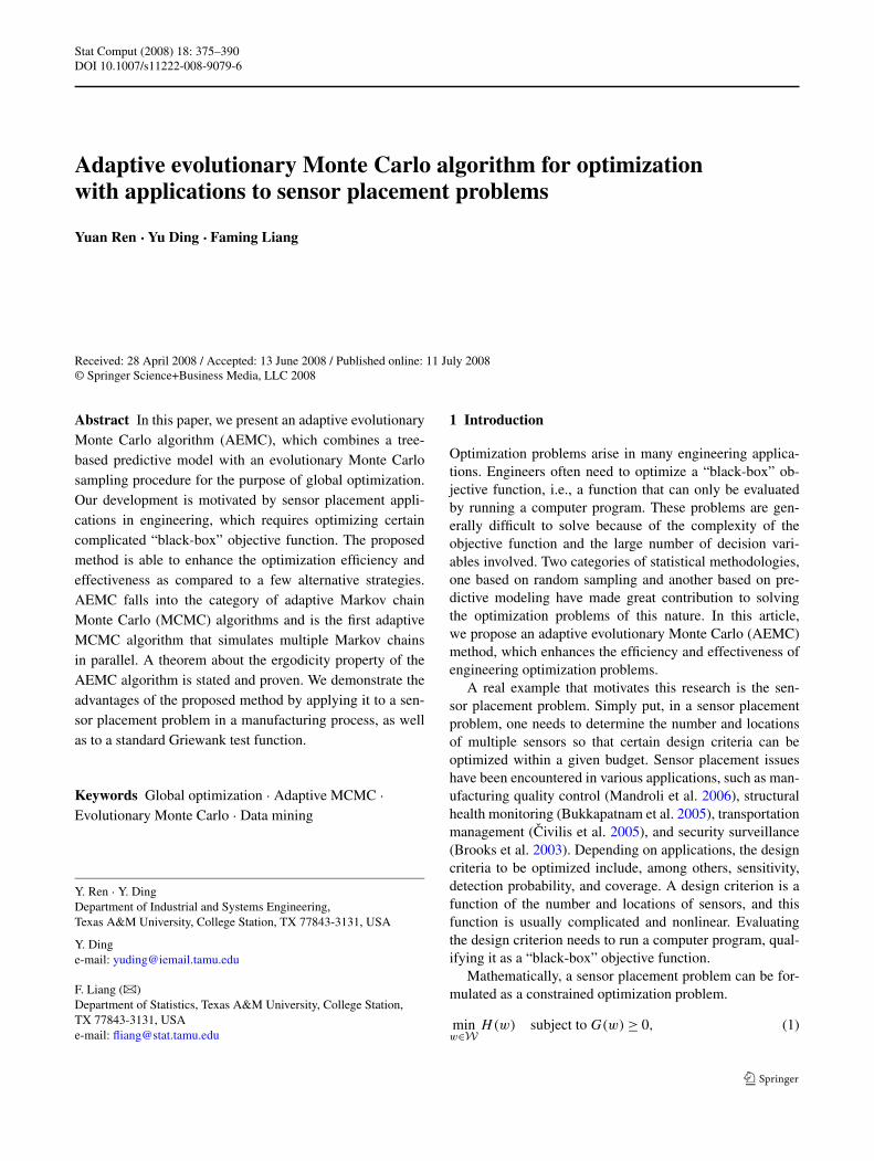
Fig. 11 Convergence rate of different algorithms
was used to obtain 105 samples and all numerical resultswere averages of 10 runs.
The Metropolis algorithm was applied with a uniformproposal distribution U [x − 2, x + 2]5. The acceptance ratewas .22. The Metropolis algorithm could not escape fromthe mode in which it started. We then compare AEMC withEMC. We only look at samples of the first dimension, sinceeach dimension is independent of each other. Since the truehistogram of the distribution is known, we can calculate theL2 distance between the estimated mass vector and the truedistribution. Specifically, we divide the interval [−10,10]into 40 intervals (with a resolution of .5), and we can calcu-late the true and estimated probability mass respectively ineach of the intervals.
All EMC related parameters are set following Liang andWong (2001). In AEMC, we set h = 25% so that samplesfrom both modes can be obtained. If h is too small, AEMCwill focus only on the peaks of the function and thus onlysamples around the mode 5 can be obtained (this is becausethe probability of sampling around the mode 5 is twice aslarge as the mode 0). In EMC, we employ the mutation andcrossover operators used in Liang and Wong (2001). The ac-ceptance rates of mutation and crossover operators were .22and .44, respectively. In AEMC, the acceptance rates of mu-tation, crossover, and data-mining operators were .23, .54,and .10, respectively. The Fig. 11 shows the L2 distance ver-sus the number of samples for the three methods in compar-ison. AEMC converges faster than EMC and the Metropo-lis algorithm, and its sampling quality is far better than theMetropolis algorithm and it also achieves better samplingquality than EMC.
5 Conclusions
In this paper, we have presented an AEMC algorithm foroptimization problems with “black-box” objective function,
which are often encountered in engineering designs (e.g.,a sensor placement problem in an assembly process). Ourexperience indicates that hybridizing a predictive modelwith an evolutionary Monte Carlo method could improvethe convergence rate for an optimization procedure. Wehave also shown that the algorithm maintains the ergodic-ity, implying its convergence to the global optimum. Nu-merical studies are used to compare the proposed AEMCmethod with other alternatives. All methods in comparisonare used to solve a sensor placement problem and to opti-mize a Griewank function. In these studies, AEMC outper-forms other alternatives and shows a much enhanced con-vergence rate.
This paper focuses mainly on the application of AEMCin solving optimization problems. Yet considering that theAEMC algorithm is an adaptive MCMC method, it shouldalso be useful for sampling from complicated probabilitydistributions. The EMC algorithm has already been shownto be a powerful tool as a sampling method. We believe thatthe data-mining component could further improve the con-vergence rate to the target distribution without destroyingthe ergodicity of the algorithm. We demonstrated the effec-tiveness of AEMC for sampling purposes using a mixtureGaussian distribution.
In the current version of AEMC, we use CART as themetamodeling method; consequently the sample space issliced into rectangles. When the function surface is com-plex, a rectangular partition may not be sufficient. A moresophisticated partition may be required. However, a goodreplacement for CART may not be straightforward to findbecause any viable candidate must be computationally effi-cient so as not to slow down the optimization process. Someother data-mining or predictive modeling methods, such asneural networks, may have more “learning” power, but theyare computationally much more expensive and are there-fore less likely to be a good candidate for the AEMC al-gorithm.
Acknowledgements The authors would like to gratefully acknowl-edge financial support from the NSF under grants CMMI-0348150 andCMMI-0726939. The authors also appreciate the editors and the refer-ees for their valuable comments and suggestions.
Appendix
We first describe the crossover, mutation, and exchange op-erators used in the EMC algorithm in Appendix A. In Ap-pendix B, we then give a brief summary of the publishedresults on the convergence of adaptive MCMC algorithms.In Appendix C, we prove the ergodicity of the AEMC algo-rithm.

Stat Comput (2008) 18: 375–390 387
Appendix A: Operators in the EMC algorithm
A.1 Crossover
From the current population x(k) = {x(k)1 , . . . , x
(k)n }, we first
select one parental pair, say x(k)i and x
(k)j (i �= j ). The first
parental sample is chosen according to a roulette wheel pro-cedure with Boltzmann weights. Then the second parentalsample is chosen randomly from the rest of the population.So the probability of selecting the pair (x
(k)i , x
(k)j ) is
P((x(k)i , x
(k)j )|x(k))
= 1
(n − 1)G(x(k))
×[exp{−H(x
(k)i )/τs} + exp{−H(x
(k)j )/τs}
], (8)
where G(x(k)) = ∑ni=1 exp{−H(x
(k)i )/τs}, and τs is the se-
lection temperature.Two offsprings are generated by some crossover opera-
tor, and the offspring with a smaller fitness value is denotedas yj and the other is yi . All the crossover operators used ingenetic algorithm, e.g., 1-point crossover, 2-point crossoverand real crossover, could be used here. Then the new pop-ulation y = {x(k)
1 , . . . , yi, . . . , yj , . . . , x(k)n } is accepted with
probability min(1,rc),
rc = f (y)
f (x(k))
T (x(k)|y)
T (y|x(k))
= exp{−(H(yi) − H(x(k)i ))/ti − (H(yj ) − H(x
(k)j ))/tj }
× T (x(k)|y)
T (y|x(k)),
where T (·|·) is the transition probability between popu-lations, and T (y|x) = P((xi, xj )|x) · P((yi, yj )|(xi, xj ))
for any two populations x and y. If the proposal is ac-cepted, the population x(k+1) = y, otherwise x(k+1) = x(k).Note that all the crossover operators are symmetric, i.e.,P((yi, yj )|(xi, xj )) = P((xi, xj )|(yi, yj )). So T (x|y)/
T (y|x) = P((yi, yj )|y)/P ((xi, xj )|x), which can be cal-culated according to (8).
Following the above selection procedure, samples withbetter H(·) values have a higher probability to be selected.Offspring generated by these parents will likely to be goodas well. In other words, the offspring have learned from thegood parents. So crossover operator allows us to constructbetter proposal distributions, and new samples generated byit are more likely to have better objective H(·) values.
A.2 Mutation
A sample, say x(k)i , is randomly selected from the current
population x(k), then mutated to a new sample yi by re-versing the values of some randomly chosen bits. Then the
new population y = {x(k)1 , . . . , yi, . . . , x
(k)n } is accepted with
probability min(1, rm),
rm = f (y)
f (x(k))
T (x(k)|y)
T (y|x(k))
= exp{−(H(yi) − H(x(k)i ))/ti}T (x(k)|y)
T (y|x(k)).
The 1-point, 2-point, and uniform mutation are all sym-metric operators, and thus T (y|x(k)) = T (x(k)|y). If theproposal is accepted, the population x(k+1) = y, otherwisex(k+1) = x(k).
A.3 Exchange
Given the current population x(k) and the temperature lad-der t , we try to change (x(k), t) = (x
(k)1 , t1, . . . , x
(k)i , ti , . . . ,
x(k)j , tj , . . . , x
(k)n , tn) to (x′, t) = (x
(k)1 , t1, . . . , x
(k)j , ti , . . . ,
x(k)i , tj , . . . , x
(k)n , tn). The new population x′ is accepted
with probability min(1,re), where
re = f (x′)f (x(k))
T (x(k)|x′)T (x ′|x(k))
= exp
{(H(x
(k)i ) − H(x
(k)j ))
(1
ti− 1
tj
)}T (x(k)|x′)T (x′|x(k))
.
If this proposal is accepted, x(k+1) = x′, otherwise x(k+1) =x(k). Typically, the exchange is performed only on stateswith neighboring temperature values, i.e., |i − j | = 1. Letp(x
(k)i ) be the probability that x
(k)i is chosen to exchange
with another state, and w(x(k)j |x(k)
i ) be the probability
that x(k)j is chosen to exchange with x
(k)i . So j = i ± 1,
and w(x(k)i+1|x(k)
i ) = w(x(k)i−1|x(k)
i ) = .5 and w(x(k)2 |x(k)
1 ) =w(x
(k)n−1|x(k)
n ) = 1. The transition probability T (x′|x(k)) =p(x
(k)i ) · w(x
(k)j |x(k)
i ) + p(x(k)j ) · w(x
(k)i |x(k)
j ), and thus
T (x′|x(k)) = T (x(k)|x′).
Appendix B: Published results on the convergenceof adaptive MCMC algorithms
In this section, we briefly review the results presented inRoberts and Rosenthal (2007). Let f (·) be a target proba-bility distribution on a state space X n with B X n = B X ×· · · × B X being the σ -algebra generated by measurable rec-tangles. Let {Kγ }γ∈Y be a collection of Markov chain ker-nels on X n, each of which has f (·) as a stationary dis-tribution: (f Kγ )(·) = f (·). Assume Kγ is φ-irreducibleand aperiodic, and we have that Kγ is ergodic for f (·),i.e., for all x ∈ X n, limk→∞ ‖Kk
γ (x, ·) − f (·)‖ = 0, where‖μ(·) − ν(·)‖ = supB∈B X n |μ(B) − ν(B)| is the usual total

388 Stat Comput (2008) 18: 375–390
variation distance. Note that B = B1 ×· · ·×Bn is a measur-able rectangle in X n, each Bi ∈ B X .
For k = 0,1,2, . . . , we have a X n-valued random vari-able X(k) representing the state of the Markov chain at it-eration k, and Y -values random variable Γ (k) representingthe kernel to be used when updating X(k) to X(k+1). LetA(k)((x, γ ),B) = P[X(k) ∈ B|X(0) = x,Γ (0) = γ ], B ∈B X n , which represents the conditional probability of X(k)
for the adaptive MCMC, given the initial conditions X(0) =x and Γ (0) = γ . Then let
T (x, γ, k) = ‖A(k)((x, γ ), ·) − f (·)‖≡ sup
B∈B X n
|A(k)((x, γ ),B) − f (B)|
denote the total variation distance between the f (·) and thedistribution of the adaptive MCMC algorithm at iteration k.Then the adaptive algorithm is called ergodic if
limk→∞T (x, γ, k) = 0, for all x ∈ X n and γ ∈ Y .
The following states three conditions that are used toprove the ergodicity of an adaptive MCMC algorithm.
(A1) (Strongly aperiodic minorisation condition) There isa C ∈ X n, ϕ > 0, and for each γ ∈ Y , there exists aprobability measure νγ (·) on X n such that
Kγ (x,B) ≥ ϕνγ (B), ∀x ∈ C, ∀B ∈ B X n . (9)
(A2) (Geometric drift condition) There is V : X n → [1,∞),0 < λ < 1, b < ∞, and supC V = v < ∞ such that foreach γ ∈ Y
Kγ V (x) ≤ λV + bI (x ∈ C), ∀x ∈ X n (10)
where Kγ V (x) = ∫X n Kγ (x,y)V (y)dy.
(A3) (Diminishing adaptation condition) The diminishingadaptation condition holds if
limk→∞ sup
x∈X n
‖KΓk+1(x, ·) − KΓk(x, ·)‖ = 0. (11)
We then have:
Theorem 2 Consider an adaptive MCMC algorithm witha family of Markov chain kernels {Kγ }γ∈Y satisfying theconditions (A1), (A2) and (A3), and E[V (x)] < ∞. Thenthe adaptive algorithm is ergodic.
Appendix C: Proof of ergodicity of AEMC
As stated in Theorem 1, we have the following:If X is compact, 0 < r < 1, and limk→∞ Pk = 0, then
AEMC is ergodic, i.e., the samples x(k) converge in distrib-ution to f (x).
Proof Denote the Markov chain kernel in the data-miningmode at iteration k by K
(1)Γk
(x, ·). To prove ergodicity, weneed to prove the conditions (A1), (A2) and (A3) for theK
(1)Γk
(x, ·), k = 0,1,2, . . . . For notational simplicity, we
drop the subscript k in the proof, denoting K(1)Γk
by K(1)Γ and
x(k) by x. We denote the proposal density learned by CARTby qΓ (·) afterwards. Since we use the Metropolis-within-Gibbs procedure in the data mining mode, we have
K(1)Γ (x,y) = K
(1,1)Γ ((x1, x2, . . . , xn),(y1, x2, . . . , xn))× · · ·
× K(1,n)Γ ((y1, . . . , yn−1, xn),
(y1, . . . , yn−1, yn)), (12)
where K(1,i)Γ (·, ·) is the Metropolis-Hastings kernel for the
transition of the i-th sample of the population and can bewritten as
K(1,i)Γ (xi, yi |ξ i )
Δ= K(1,i)Γ ((y1, . . . , yi−1, xi, . . . , xn),
(y1, . . . , yi, xi+1, . . . , xn))
= sΓ (xi, yi |ξ i ) + I (xi = yi)
(1 −
∫
XsΓ (xi, z|ξ i )dz
).
(13)
Here ξ i = (y1, . . . , yi−1, xi+1, . . . , xn) denotes the collec-tion of the fixed samples in the transition, sΓ (xi, yi |ξ i ) =qΓ (yi)min{1,
p(yi |ξ i )qΓ (xi )
p(xi |ξ i )qΓ (yi )}, and p(z|ξ ) is the conditional
density of z given the other components ξ .Since we have assumed that X n is compact, it is natural
to assume that f (x) is bounded away from 0 and ∞ on thespace X n. As long as 0 < r < 1, we have that the proposalqΓ (z) is bounded away from 0 due to (6), and then we havethe minorisation condition, i.e.,
ω∗ = supy∈X
p(y|ξ)
qΓ (y)< ∞. (14)
And then
K(1,i)Γ (z,Bi |ξ i )
=∫
Bi
sΓ (z, y|ξ i )dy
+ I (z ∈ Bi)
(1 −
∫
XsΓ (z,w|ξ i )dw
)
≥∫
Bi
qΓ (y)min
{1,
p(y|ξ i )qΓ (z)
p(z|ξ i )qΓ (y)
}dy
=∫
Bi
min
{qΓ (y),
p(y|ξ i )qΓ (z)
p(z|ξ i )
}dy

Stat Comput (2008) 18: 375–390 389
≥∫
Bi
min
{qΓ (y),
p(y|ξ i )
ω∗
}dy (by (14))
=∫
Bi
p(y|ξ i )
ω∗ dy (by definition of ω∗)
≥∫
Bi
p∗i (y)
ω∗ dy
(by defining p∗i (y) = inf
ξ′i∈X n−1p(y|ξ ′
i ))
= p∗i (Bi)
ω∗ .
Since we have assumed that f (x) is bounded away from 0and ∞, p(y|ξi), as the conditional density of a componentof x, is bounded away from 0 and ∞, and so are p∗
i (y) andp∗
i (Bi). Therefore, we have the following results:
K(1)Γ (x,B)
=∫
B1
· · ·∫
Bn
K(1,1)Γ (x1, y1|ξ1) × · · ·
× K(1,n)Γ (xn, yn|ξn)dy1 · · ·dyn
≥ p∗n(Bn)
ω∗
∫
B1
· · ·∫
Bn−1
K(1,1)Γ (x1, y1|ξ1) × · · ·
× K(1,n−1)Γ (xn−1, yn−1|ξn−1)dy1 · · ·dyn−1
· · ·
≥n∏
i=1
p∗i (Bi)/(ω
∗)n.
Define νΓ (B) = ∏ni=1 p∗
i (Bi) and ϕ = 1/(ω∗)n, and thenwe have
K(1)Γ (x,B) ≥ ϕνΓ (B), ∀x ∈ X n, ∀B ∈ B X n . (15)
The equation (15) implies that the condition (A1) is satisfied,and it also implies that C = X n is a small set (Mengersenand Tweedie 1996) and that the following condition holds:
K(1)Γ V (x) ≤ λV (x) + bI (x ∈ C), ∀x ∈ X n, (16)
by choosing V (x) = 1, 0 < λ < 1, b = 1−λ. Then the equa-tion (16) implies that the condition (A2) is satisfied. Also wehave E[V (x)] < ∞.
Now we prove the Diminishing Adaptation condition forthe kernel K
(1)Γ . Suppose at iteration k +1 the newly learned
data-mining proposal is K(1)Γ ∗ , then
K(1)Γk+1
= Pk+1K(1)Γ ∗ + (1 − Pk+1)K
(1)Γk
.
Then we have ‖K(1)Γk+1
−K(1)Γk
‖ = Pk+1‖K(1)Γ ∗ −K
(1)Γk
‖. Sincelimk→∞ Pk = 0, to prove the equation (11), it suffices toprove that ‖K(1)
Γ ∗ − K(1)Γk
‖ is bounded. Since both K(1)Γ ∗ and
K(1)Γk
are Markov chain kernels, we have ‖K(1)Γ ∗ −K
(1)Γk
‖ ≤ 2,and
‖K(1)Γk+1
− K(1)Γk
‖ = Pk+1‖K(1)Γ ∗ − K
(1)Γk
‖ ≤ 2Pk+1 → 0.
This proves the diminishing adaptation condition.The proof is complete. �
References
Andrieu, C., Robert, C.P.: Controlled MCMC for optimal sampling.MCMC Preprint Service. http://www.ceremade.dauphine.fr/~xian/control.ps.gz (2002)
Atchadé, Y.F., Rosenthal, J.S.: On adaptive Markov chain Monte Carloalgorithms. Bernoulli 11, 815–828 (2005)
Bertsimas, D., Tsitsiklis, J.: Simulated annealing. Stat. Sci. 8, 10–15(1993)
Breiman, L., Friedman, J.H., Olshen, R.A., Stone, C.J.: Classificationand Regression Trees. Chapman & Hall, New York (1984)
Brockwell, A.E., Kadane, J.B.: Identification of regeneration times inMCMC simulation, with application to adaptive schemes. J. Com-put. Graph. Stat. 14, 436–458 (2005)
Brooks, R.R., Ramanathan, P., Sayeed, A.M.: Distributed target clas-sification and tracking in sensor networks. Proc. IEEE 91, 1163–1171 (2003)
Box, G.E.P., Wilson, K.B.: On the experimental attainment of optimumconditions. J. R. Stat. Soc. B Stat. Methodol. 13, 1–45 (1951)
Bukkapatnam, S.T.S., Nichols, J.M., Seaver, M., Trickey, S.T., Hunter,M.: A wavelet-based, distortion energy approach to structuralhealth monitoring. Struct. Health Monitor. J. 4, 247–258 (2005)
Chen, V.C.P., Tsui, K., Barton, R.R., Meckesheimer, M.: A review ondesign, modeling and applications of computer experiments. IIETrans. 38, 273–291 (2006)
Civilis, A., Jensen, C.S., Pakalnis, S.: Techniques for efficient trackingof road-network-based moving objects. IEEE Trans. Knowl. DataEng. 17, 698–712 (2005)
Fang, K., Li, R., Sudjianto, A.: Design and modeling for computer ex-periments. Chapman & Hall/CRC, Boca Raton (2006)
Geman, S., Geman, D.: Stochastic relaxation, Gibbs distribution andthe Bayesian restoration of images. IEEE Trans. Pattern Anal. 6,721–741 (1984)
Gilks, W.R., Richardson, S., Spiegelhalter, D.J.: Introducing Markovchain Monte Carlo. In: Markov Chain Monte Carlo in Practice,pp. 1–19. Chapman & Hall, London (1995)
Gilks, W.R., Roberts, G.O., Sahu, S.K.: Adaptive Markov chain MonteCarlo through regeneration. J. Am. Stat. Assoc. 93, 1045–1054(1998)
Griewank, A.O.: Generalized descent for global optimization. J. Op-tim. Theory Appl. 34, 11–39 (1981)
Guikema, S.D., Davidson, R.A., Çagnan, Z.: Efficient simulation-based discrete optimization. In: Ingalls, R.G., Rossetti, M.D.,Smith, J.S., Peters, B.A. (eds.) Proceedings of the 2004 WinterSimulation Conference (2004)
Haario, H., Saksman, E., Tamminen, J.: An adaptive metropolis algo-rithm. Bernoulli 7, 223–242 (2001)
Hastie, T., Tibshirani, R., Friedman, J.: The Elements of StatisticalLearning. Springer, New York (2001)
Holland, J.H.: Adaptation in Natural and Artificial Systems: An In-troductory Analysis with Applications to Biology, Control, andArtificial Intelligence. MIT Press, Cambridge (1992)
Huyet, A.L.: Optimization and analysis aid via data-mining for simu-lated production systems. Eur. J. Oper. Res. 173, 827–838 (2006)
Jin, J., Shi, J.: State space modeling of sheet metal assembly for di-mensional control. J. Manuf. Sci. Eng. 121, 756–762 (1999)

390 Stat Comput (2008) 18: 375–390
Liang, F.: A generalized Wang-Landau algorithm for Monte Carlocomputation. J. Am. Stat. Assoc. 100, 1311–1327 (2005)
Liang, F., Liu, C., Carroll, R.J.: Stochastic approximation in MonteCarlo Computation. J. Am. Stat. Assoc. 102, 305–320 (2007)
Liang, F., Wong, W.H.: Evolutionary Monte Carlo: applications to Cp
model sampling and change point problem. Stat. Sin. 10, 317–342(2000)
Liang, F., Wong, W.H.: Real-parameter evolutionary Monte Carlo withapplications to Bayesian mixture models. J. Am. Stat. Assoc. 96,653–666 (2001)
Liu, H., Igusa, T.: Feature-based classification for design optimization.Res. Eng. Des. 17, 189–206 (2007)
Kim, P., Ding, Y.: Optimal engineering system design guided by data-mining methods. Technometrics 47, 336–348 (2005)
Liu, C., Ding, Y., Chen, Y.: Optimal coordinate sensor placements forestimating mean and variance components of variation sources.IIE Trans. 37, 877–889 (2005)
Mandroli, S.S., Shrivastava, A.K., Ding, Y.: A survey of inspectionstrategy and sensor distribution studies in discrete-part manufac-turing processes. IIE Trans. 38, 309–328 (2006)
Mengersen, K.L., Tweedie, R.L.: Rates of convergence of the Hastingsand Metropolis algorithms. Ann. Stat. 24, 101–121 (1996)
Michalski, R.S.: Learnable evolution model: evolutionary processesguided by machine learning. Mach. Learn. 38, 9–40 (2000)
Müller, P.: A generic approach to posterior integration and Gibbs sam-pling. Technical Report, Purdue University, West Lafayette, Indi-ana (1991)
Neal, R.M.: Bayesian learning for neural networks. Lecture Notes inStatistics, vol. 118. Springer, New York (1996)
Roberts, G.O., Rosenthal, J.S.: General state-space Markov chains andMCMC algorithms. Probab. Surv. 1, 20–71 (2004)
Roberts, G.O., Rosenthal, J.S.: Coupling and ergodicity of adaptiveMarkov chain Monte Carlo algorithms. J. Appl. Probab. 44, 458–475 (2007)
Roberts, G.O., Tweedie, R.L.: Geometric convergence and central limittheorems for multidimensional Hastings and Metropolis algo-rithms. Biometrika 83, 95–110 (1996)
Rosenthal, J.S.: Minorization conditions and convergence rate forMarkov chain Monte Carlo. J. Am. Stat. Assoc. 90, 558–566(1995)
Sacks, J., Welch, W.J., Mitchell, T.J., Wynn, H.P.: Design and analysisof computer experiments. Stat. Sci. 4, 409–435 (1989)
Schwabacher, M., Ellman, T., Hirsh, H.: Learning to set up numeri-cal optimizations of engineering designs. In: Braha, D. (ed.) DataMining for Design and Manufacturing, pp. 87–125. Kluwer Aca-demic, Dordrecht (2001)
Simpson, T.W., Peplinski, J., Koch, P.N., Allen, J.K.: On the useof statistics in design and the implications for deterministiccomputer experiments. In: Design Theory and Methodology—DTM’97, Sacramento, CA, September 14–17, ASME, Paper No.DETC97/DTM-3881 (1997)
Wong, W.H., Liang, F.: Dynamic weighting in Monte Carlo and opti-mization. Proc. Natl. Acad. Sci. USA 94, 14220–14224 (1997)