Embed Size (px)
Citation preview
STAT 6720
Mathematical Statistics II
Spring Semester 2000
Dr. J�urgen Symanzik
Utah State University
Department of Mathematics and Statistics
3900 Old Main Hill
Logan, UT 84322{3900
Tel.: (435) 797{0696
FAX: (435) 797{1822
e-mail: [email protected]

Contents
Acknowledgements 1
6 Limit Theorems (Continued from Stat 6710) 1
6.4 Central Limit Theorems . . . . . . . . . . . . . . . . . . . . . . . . . . . . . . . . . . 1
7 Sample Moments 8
7.1 Random Sampling . . . . . . . . . . . . . . . . . . . . . . . . . . . . . . . . . . . . . 8
7.2 Sample Moments and the Normal Distribution . . . . . . . . . . . . . . . . . . . . . 11
8 The Theory of Point Estimation 16
8.1 The Problem of Point Estimation . . . . . . . . . . . . . . . . . . . . . . . . . . . . . 16
8.2 Properties of Estimates . . . . . . . . . . . . . . . . . . . . . . . . . . . . . . . . . . 17
8.3 Su�cient Statistics . . . . . . . . . . . . . . . . . . . . . . . . . . . . . . . . . . . . . 19
8.4 Unbiased Estimation . . . . . . . . . . . . . . . . . . . . . . . . . . . . . . . . . . . . 27
8.5 Lower Bounds for the Variance of an Estimate . . . . . . . . . . . . . . . . . . . . . 37
8.6 The Method of Moments . . . . . . . . . . . . . . . . . . . . . . . . . . . . . . . . . . 45
8.7 Maximum Likelihood Estimation . . . . . . . . . . . . . . . . . . . . . . . . . . . . . 46
8.8 Decision Theory | Bayes and Minimax Estimation . . . . . . . . . . . . . . . . . . . 53
9 Hypothesis Testing 60
9.1 Fundamental Notions . . . . . . . . . . . . . . . . . . . . . . . . . . . . . . . . . . . . 60
9.2 The Neyman{Pearson Lemma . . . . . . . . . . . . . . . . . . . . . . . . . . . . . . . 65
9.3 Monotone Likelihood Ratios . . . . . . . . . . . . . . . . . . . . . . . . . . . . . . . . 68
9.4 Unbiased and Invariant Tests . . . . . . . . . . . . . . . . . . . . . . . . . . . . . . . 72
10 More on Hypothesis Testing 86
10.1 Likelihood Ratio Tests . . . . . . . . . . . . . . . . . . . . . . . . . . . . . . . . . . . 86
10.2 Parametric Chi{Squared Tests . . . . . . . . . . . . . . . . . . . . . . . . . . . . . . 91
10.3 t{Tests and F{Tests . . . . . . . . . . . . . . . . . . . . . . . . . . . . . . . . . . . . 95
10.4 Bayes and Minimax Tests . . . . . . . . . . . . . . . . . . . . . . . . . . . . . . . . . 99
1
11 Con�dence Estimation 105
11.1 Fundamental Notions . . . . . . . . . . . . . . . . . . . . . . . . . . . . . . . . . . . . 105
11.2 Shortest{Length Con�dence Intervals . . . . . . . . . . . . . . . . . . . . . . . . . . . 109
11.3 Con�dence Intervals and Hypothesis Tests . . . . . . . . . . . . . . . . . . . . . . . . 114
11.4 Bayes Con�dence Intervals . . . . . . . . . . . . . . . . . . . . . . . . . . . . . . . . . 120
12 Nonparametric Inference 121
12.1 Nonparametric Estimation . . . . . . . . . . . . . . . . . . . . . . . . . . . . . . . . . 121
12.2 Single-Sample Hypothesis Tests . . . . . . . . . . . . . . . . . . . . . . . . . . . . . . 128
13 Some Results from Sampling 131
13.1 Simple Random Samples . . . . . . . . . . . . . . . . . . . . . . . . . . . . . . . . . . 131
13.2 Strati�ed Random Samples . . . . . . . . . . . . . . . . . . . . . . . . . . . . . . . . 134
14 Some Results from Sequential Statistical Inference 138
14.1 Fundamentals of Sequential Sampling . . . . . . . . . . . . . . . . . . . . . . . . . . 138
14.2 Sequential Probability Ratio Tests . . . . . . . . . . . . . . . . . . . . . . . . . . . . 143
Index 146
2
Acknowledgements
I would like to thank my students, Hanadi B. Eltahir, Rich Madsen, and Bill Morphet, who helped
in typesetting these lecture notes using LATEX and for their suggestions how to improve some of the
material presented in class.
In addition, I particularly would like to thank Mike Minnotte and Dan Coster, who previously
taught this course at Utah State University, for providing me with their lecture notes and other
materials related to this course. Their lecture notes, combined with additional material from
Rohatgi (1976) and other sources listed below, form the basis of the script presented here.
The textbook required for this class is:
� Rohatgi, V. K. (1976): An Introduction to Probability Theory and Mathematical Statistics,
John Wiley and Sons, New York, NY.
A Web page dedicated to this class is accessible at:
http://www.math.usu.edu/~symanzik/teaching/2000_stat6720/stat6720.html
This course closely follows Rohatgi (1976) as described in the syllabus. Additional material origi-
nates from the lectures from Professors Hering, Trenkler, Gather, and Kreienbrock I have attended
while studying at the Universit�at Dortmund, Germany, the collection of Masters and PhD Prelim-
inary Exam questions from Iowa State University, Ames, Iowa, and the following textbooks:
� Bandelow, C. (1981): Einf�uhrung in die Wahrscheinlichkeitstheorie, Bibliographisches Insti-
tut, Mannheim, Germany.
� B�uning, H., and Trenkler, G. (1978): Nichtparametrische statistische Methoden, Walter de
Gruyter, Berlin, Germany.
� Casella, G., and Berger, R. L. (1990): Statistical Inference, Wadsworth & Brooks/Cole, Paci�c
Grove, CA.
� Fisz, M. (1989): Wahrscheinlichkeitsrechnung und mathematische Statistik, VEB Deutscher
Verlag der Wissenschaften, Berlin, German Democratic Republic.
� Kelly, D. G. (1994): Introduction to Probability, Macmillan, New York, NY.
� Lehmann, E. L. (1983): Theory of Point Estimation (1991 Reprint), Wadsworth & Brooks/Cole,
Paci�c Grove, CA.
� Lehmann, E. L. (1986): Testing Statistical Hypotheses (Second Edition { 1994 Reprint),
Chapman & Hall, New York, NY.
3
� Mood, A. M., and Graybill, F. A., and Boes, D. C. (1974): Introduction to the Theory of
Statistics (Third Edition), McGraw-Hill, Singapore.
� Parzen, E. (1960): Modern Probability Theory and Its Applications, Wiley, New York, NY.
� Searle, S. R. (1971): Linear Models, Wiley, New York, NY.
� Tamhane, A. C., and Dunlop, D. D. (2000): Statistics and Data Analysis { From Elementary
to Intermediate, Prentice Hall, Upper Saddle River, NJ.
Additional de�nitions, integrals, sums, etc. originate from the following formula collections:
� Bronstein, I. N. and Semendjajew, K. A. (1985): Taschenbuch der Mathematik (22. Au age),
Verlag Harri Deutsch, Thun, German Democratic Republic.
� Bronstein, I. N. and Semendjajew, K. A. (1986): Erg�anzende Kapitel zu Taschenbuch der
Mathematik (4. Au age), Verlag Harri Deutsch, Thun, German Democratic Republic.
� Sieber, H. (1980): Mathematische Formeln | Erweiterte Ausgabe E, Ernst Klett, Stuttgart,
Germany.
J�urgen Symanzik, January 19, 2001
4
Stat 6720 Mathematical Statistics II Spring Semester 2000
Lecture 2: Wednesday 1/12/2000
Scribe: J�urgen Symanzik
6 Limit Theorems (Continued from Stat 6710)
6.4 Central Limit Theorems
Let fXng1n=1 be a sequence of rv's with cdf's fFng1n=1. Suppose that the mgf Mn(t) of Xn exists.
Questions: Does Mn(t) converge? Does it converge to a mgfM(t)? If it does converge, does it hold
that Xn
d�! X for some rv X?
Example 6.4.1:
Let fXng1n=1 be a sequence of rv's such that P (Xn = �n) = 1. Then the mgf isMn(t) = E(etX ) =
e�tn. So
limn!1
Mn(t) =
8>><>>:0; t > 0
1; t = 0
1; t < 0
So Mn(t) does not converge to a mgf and Fn(x)! F (x) = 1 8x. But F (x) is not a cdf.
Note:
Due to Example 6.4.1, the existence of mgf's Mn(t) that converge to something is not enough to
conclude convergence in distribution.
Conversely, suppose that Xn has mgf Mn(t), X has mgf M(t), and Xn
d�! X. Does it hold that
Mn(t)!M(t)?
Not necessarily! See Rohatgi, page 277, Example 2, as a counter example. Thus, convergence in
distribution of rv's that all have mgf's does not imply the convergence of mgf's.
However, we can make the following statement in the next Theorem:
Theorem 6.4.2: Continuity Theorem
Let fXng1n=1 be a sequence of rv's with cdf's fFng1n=1 and mgf's fMn(t)g1n=1. Suppose that Mn(t)
exists for j t j� t0 8n. If there exists a rv X with cdf F and mgfM(t) which exists for j t j� t1 < t0
such that limn!1
Mn(t) =M(t) 8t 2 [�t1; t1], then Fnw�! F , i.e., Xn
d�! X.
1
Example 6.4.3:
Let Xn � Bin(n; �n). Recall (e.g., from Theorem 3.3.12 and related Theorems) that for
X � Bin(n; p) the mgf is MX(t) = (1� p+ pet)n. Thus,
Mn(t) = (1� �
n+�
net)n = (1 +
�(et � 1)
n)n
(�)�! e�(et�1) as n!1:
In (�) we use the fact that limn!1
(1 +x
n)n = ex. Recall that e�(e
t�1) is the mgf of a rv X where
X � Poisson(�). Thus, we have established the well{known result that the Binomial distribution
approaches the Poisson distribution, given that n!1 in such a way that np = � > 0.
Note:
Recall Theorem 3.3.11: Suppose that fXng1n=1 is a sequence of rv's with characteristic fuctions
f�n(t)g1n=1. Suppose that
limn!1
�n(t) = �(t) 8t 2 (�h; h) for some h > 0;
and �(t) is the characteristic function of a rv X. Then Xn
d�! X.
Theorem 6.4.4: Lindeberg{L�evy Central Limit Theorem
Let fXng1n=1 be a sequence of iid rv's with E(Xi) = � and 0 < V ar(Xi) = �2 <1. Then it holds
for Xn =1n
nXi=1
Xi that
pn(Xn � �)
�
d�! Z
where Z � N(0; 1).
Proof:
Let Z � N(0; 1). According to Theorem 3.3.12 (v), the characteristic function of Z is
�Z(t) = exp(�12 t2).
Let �(t) be the characteristic function of Xi. We now determine the characteristic function �n(t)
ofpn(Xn��)
�:
�n(t) = E
0BBBB@exp0BBBB@it
pn( 1
n
nXi=1
Xi � �)
�
1CCCCA1CCCCA
=
Z 1
�1: : :
Z 1
�1exp
0BBBB@itpn( 1
n
nXi=1
Xi � �)
�
1CCCCAdFX
2
= exp(� itpn�
�)
Z 1
�1exp(
itx1pn�
)dFX1: : :
Z 1
�1exp(
itxnpn�
)dFXn
=
��(
tpn�
) exp(� it�pn�
)
�nRecall from Theorem 3.3.5 that if the kth moment exists, then �(k)(0) = ikE(Xk). Thus, if we
develop a Taylor series for �( tpn�) around t = 0, we get:
�(tpn�
) = �(0) + t�0(0) +1
2t2�00(0) +
1
6t3�000(0) + : : :
= 1 + ti�pn�
� 1
2t2�2 + �2
n�2+ o
�(
tpn�
)2�
Here we make use of the Landau symbol \o". In general, if we write u(x) = o(v(x)) for x! L,
this implies limx!L
u(x)
v(x)= 0, i.e., u(x) goes to 0 faster than v(x) or v(x) goes to 1 faster than u(x).
We say that u(x) is of smaller order than v(x) as x! L. Examples are 1x3
= o( 1x2) and x2 = o(x3)
for x!1. See Rohatgi, page 6, for more details on the Landau symbols \O" and \o".
Similarly, if we develop a Taylor series for exp(� it�pn�) around t = 0, we get:
exp(� it�pn�
) = 1� ti�pn�
� 1
2t2�2
n�2+ o
�(
tpn�
)2�
Combining these results, we get:
�n(t) =
1 + t
i�pn�
� 1
2t2�2 + �2
n�2+ o
�(
tpn�
)2�!
1� ti�pn�
� 1
2t2�2
n�2+ o
�(
tpn�
)2�!!n
=
1� t
i�pn�
� 1
2t2�2
n�2+ t
i�pn�
+ t2�2
n�2� 1
2t2�2 + �2
n�2+ o
�(
tpn�
)2�!n
=
1� 1
2
t2
n+ o
�(
tpn�
)2�!n
(�)�! exp(� t2
2) as n!1
Thus, limn!1
�n(t) = �Z(t) 8t. For a proof of (�), see Rohatgi, page 278, Lemma 1. According to
the Note above, it holds that pn(Xn � �)
�
d�! Z:
3
Stat 6720 Mathematical Statistics II Spring Semester 2000
Lecture 3: Friday 1/14/2000
Scribe: J�urgen Symanzik
De�nition 6.4.5:
Let X1;X2 be iid non{degenerate rv's with common cdf F . Let a1; a2 > 0. We say that F is stable
if there exist constants A and B (depending on a1 and a2) such that B�1(a1X1 + a2X2 � A) also
has cdf F .
Note:
When generalizing the previous de�nition to sequences of rv's, we have the following examples for
stable distributions:
� Xi iid Cauchy. Then 1n
nXi=1
Xi � Cauchy (here Bn = n;An = 0).
� Xi iid N(0; 1). Then 1pn
nXi=1
Xi � N(0; 1) (here Bn =pn;An = 0).
De�nition 6.4.6:
Let fXig1i=1 be a sequence of iid rv's with common cdf F . Let Tn =nXi=1
Xi. F belongs to the domain
of attraction of a distribution V if there exist norming and centering constants fBng1n=1; Bn > 0,
and fAng1n=1 such that
P (B�1n (Tn �An) � x) = F
B�1n (Tn�An)(x)! V (x) as n!1
at all continuity points x of V .
Note:
A very general Theorem from Lo�eve states that only stable distributions can have domains of at-
traction. From the practical point of view, a wide class of distributions F belong to the domain of
attraction of the Normal distribution.
4
Theorem 6.4.7: Lindeberg Central Limit Theorem
Let fXig1i=1 be a sequence of independent non{degenerate rv's with cdf's fFig1i=1. Assume that
E(Xk) = �k and V ar(Xk) = �2k<1. Let s2n =
nXk=1
�2k.
If the Fk are absolutely continuous with pdf's fk = F 0k, assume that it holds for all � > 0 that
(A) limn!1
1
s2n
nXk=1
Zfjx��kj>�sng
(x� �k)2F 0k(x)dx = 0:
If the Xk are discrete rv's with support fxklg and probabilities fpklg, l = 1; 2; : : :, assume that it
holds for all � > 0 that
(B) limn!1
1
s2n
nXk=1
Xjxkl��kj>�sn
(xkl � �k)2pkl = 0:
The conditions (A) and (B) are called Lindeberg Condition (LC). If either LC holds, then
nXk=1
(Xk � �k)
sn
d�! Z
where Z � N(0; 1).
Proof:
Similar to the proof of Theorem 6.4.4, we can use characteristic functions again. An alternative
proof is given in Rohatgi, pages 282{288.
Note:
Feller shows that the LC is a necessary condition if�2n
s2n! 0 and s2n !1 as n!1.
Corollary 6.4.8:
Let fXig1i=1 be a sequence of iid rv's such that 1pn
nXi=1
Xi has the same distribution for all n. If
E(Xi) = 0 and V ar(Xi) = 1, then Xi � N(0; 1).
Proof:
Let F be the common cdf of 1pn
nXi=1
Xi for all n (including n = 1). By the CLT,
limn!1
P (1pn
nXi=1
Xi � x) = �(x);
where �(x) denotes P (Z � x) for Z � N(0; 1). Also, P ( 1pn
nXi=1
Xi � x) = F (x) for each n. There-
fore, we must have F (x) = �(x).
5
Note:
In general, if X1;X2; : : :, are independent rv's such that there exists a constant A with
P (j Xn j� A) = 1 8n, then the LC is satis�ed if s2n !1 as n!1. Why??
Suppose that s2n !1 as n!1. Since the j Xk j's are uniformly bounded (by A), so are the rv's
(Xk �E(Xk)). Thus, for every � > 0 there exists an N� such that if n � N� then
P (j Xk �E(Xk) j< �sn; k = 1; : : : ; n) = 1:
This implies that the LC holds since we would integrate (or sum) over the empty set, i.e., the set
fj x� �k j> �sng = �.
The converse also holds. For a sequence of uniformly bounded independent rv's, a necessary and
su�cient condition for the CLT to hold is that s2n !1 as n!1.
Example 6.4.9:
Let fXig1i=1 be a sequence of independent rv's such that E(Xk) = 0, �k = E(j Xk j2+�) < 1 for
some � > 0, andnX
k=1
�k = o(s2+�n ).
Does the LC hold? It is:
1
s2n
nXk=1
Zfjxj>�sng
x2fk(x)dx(A)
� 1
s2n
nXk=1
Zfjxj>�sng
j x j2+���s�n
fk(x)dx
� 1
s2n��s�n
nXk=1
Z 1
�1j x j2+� fk(x)dx
=1
s2n��s�n
nXk=1
�k
=1
��
0BBBB@nX
k=1
�k
s2+�n
1CCCCA(B)�! 0 as n!1
(A) holds since for j x j> �sn, it isjxj���s�n
> 1. (B) holds sincenX
k=1
�k = o(s2+�n ).
Thus, the LC is satis�ed and the CLT holds.
6
Note:
(i) In general, if there exists a � > 0 such that
nXk=1
E(j Xk � �k j2+�)
s2+�n
�! 0 as n!1;
then the LC holds.
(ii) Both the CLT and the WLLN hold for a large class of sequences of rv's fXigni=1. If the
fXig's are independent uniformly bounded rv's, i.e., if P (j Xn j� M) = 1 8n, the WLLN
(as formulated in Theorem 6.2.3) holds. The CLT holds provided that s2n !1 as n!1.
If the rv's fXig are iid, then the CLT is a stronger result than the WLLN since the CLT
provides an estimate of the probability P ( 1nj
nXi=1
Xi � n� j� �) � 1� P (j Z j� �
�
pn), where
Z � N(0; 1), and the WLLN follows. However, note that the CLT requires the existence of a
2nd moment while the WLLN does not.
(iii) If the fXig are independent (but not identically distributed) rv's, the CLT may apply while
the WLLN does not.
(iv) See Rohatgi, pages 289{293, for additional details and examples.
7
Stat 6720 Mathematical Statistics II Spring Semester 2000
Lecture 4: Wednesday 1/19/2000
Scribe: J�urgen Symanzik
7 Sample Moments
7.1 Random Sampling
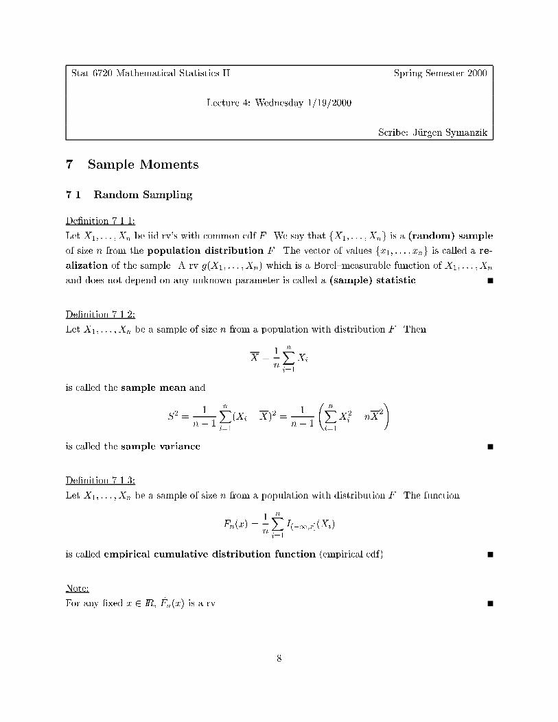
De�nition 7.1.1:
Let X1; : : : ; Xn be iid rv's with common cdf F . We say that fX1; : : : ;Xng is a (random) sample
of size n from the population distribution F . The vector of values fx1; : : : ; xng is called a re-
alization of the sample. A rv g(X1; : : : ;Xn) which is a Borel{measurable function of X1; : : : ;Xn
and does not depend on any unknown parameter is called a (sample) statistic.
De�nition 7.1.2:
Let X1; : : : ; Xn be a sample of size n from a population with distribution F . Then
X =1
n
nXi=1
Xi
is called the sample mean and
S2 =1
n� 1
nXi=1
(Xi �X)2 =1
n� 1
nXi=1
X2i � nX
2
!
is called the sample variance.
De�nition 7.1.3:
Let X1; : : : ; Xn be a sample of size n from a population with distribution F . The function
F̂n(x) =1
n
nXi=1
I(�1;x](Xi)
is called empirical cumulative distribution function (empirical cdf).
Note:
For any �xed x 2 IR, F̂n(x) is a rv.
8
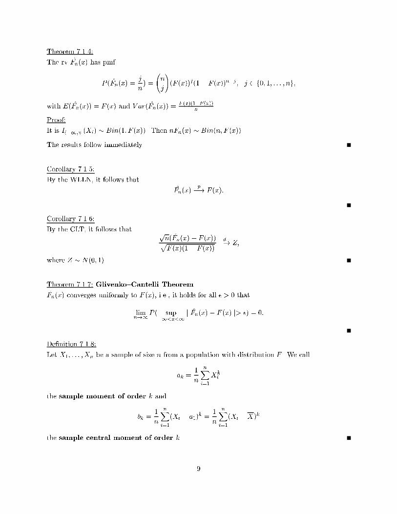
Theorem 7.1.4:
The rv F̂n(x) has pmf
P (F̂n(x) =j
n) =
n
j
!(F (x))j(1� F (x))n�j ; j 2 f0; 1; : : : ; ng;
with E(F̂n(x)) = F (x) and V ar(F̂n(x)) =F (x)(1�F (x))
n.
Proof:
It is I(�1;x](Xi) � Bin(1; F (x)). Then nF̂n(x) � Bin(n; F (x)).
The results follow immediately.
Corollary 7.1.5:
By the WLLN, it follows that
F̂n(x)p�! F (x):
Corollary 7.1.6:
By the CLT, it follows that pn(F̂n(x)� F (x))pF (x)(1 � F (x))
d�! Z;
where Z � N(0; 1).
Theorem 7.1.7: Glivenko{Cantelli Theorem
F̂n(x) converges uniformly to F (x), i.e., it holds for all � > 0 that
limn!1
P ( sup�1<x<1
j F̂n(x)� F (x) j> �) = 0:
De�nition 7.1.8:
Let X1; : : : ; Xn be a sample of size n from a population with distribution F . We call
ak =1
n
nXi=1
Xk
i
the sample moment of order k and
bk =1
n
nXi=1
(Xi � a1)k =
1
n
nXi=1
(Xi �X)k
the sample central moment of order k.
9
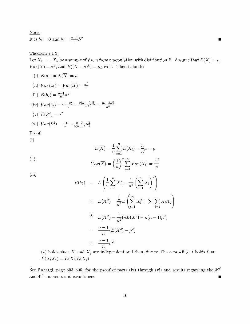
Note:
It is b1 = 0 and b2 =n�1nS2.
Theorem 7.1.9:
LetX1; : : : ;Xn be a sample of size n from a population with distribution F . Assume that E(X) = �,
V ar(X) = �2, and E((X � �)k) = �k exist. Then it holds:
(i) E(a1) = E(X) = �
(ii) V ar(a1) = V ar(X) = �2
n
(iii) E(b2) =n�1n�2
(iv) V ar(b2) =�4��22
n� 2(�4�2�22)
n2+
�4�3�22n3
(v) E(S2) = �2
(vi) V ar(S2) = �4
n� n�3
n(n�1)�22
Proof:
(i)
E(X) =1
n
nXi=1
E(Xi) =n
n� = �
(ii)V ar(X) =
�1
n
�2 nXi=1
V ar(Xi) =�2
n
(iii)
E(b2) = E
0@ 1
n
nXi=1
X2i �
1
n2
nXi=1
Xi
!21A
= E(X2)� 1
n2E
0@ nXi=1
X2i +
XXi 6=j
XiXj
1A(�)= E(X2)� 1
n2(nE(X2) + n(n� 1)�2)
=n� 1
n(E(X2)� �2)
=n� 1
n�2
(�) holds since Xi and Xj are independent and then, due to Theorem 4.5.3, it holds that
E(XiXj) = E(Xi)E(Xj).
See Rohatgi, page 303{306, for the proof of parts (iv) through (vi) and results regarding the 3rd
and 4th moments and covariances.
10
Stat 6720 Mathematical Statistics II Spring Semester 2000
Lecture 5: Friday 1/21/2000
Scribe: Rich Madsen & J�urgen Symanzik
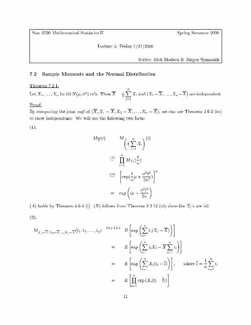
7.2 Sample Moments and the Normal Distribution
Theorem 7.2.1:
Let X1; : : : ; Xn be iidN(�; �2) rv's. Then X = 1n
nXi=1
Xi and (X1�X; : : : ;Xn�X) are independent.
Proof:
By computing the joint mgf of (X;X1 �X;X2 �X; : : : ;Xn �X), we can use Theorem 4.6.3 (iv)
to show independence. We will use the following two facts:
(1):
MX(t) = M
1n
nXi=1
Xi
!(t)(A)=
nYi=1
MXi(t
n)
(B)=
"exp(
t
n�+
�2t2
2n2)
#n
= exp
t�+
�2t2
2n
!
(A) holds by Theorem 4.6.4 (i). (B) follows from Theorem 3.3.12 (vi) since the Xi's are iid.
(2):
MX1�X;X2�X;:::;Xn�X(t1; t2; : : : ; tn)
Def:4:6:1= E
"exp
nXi=1
ti(Xi �X)
!#
= E
"exp
nXi=1
tiXi �X
nXi=1
ti
!#
= E
"exp
nXi=1
Xi(ti � t)
!#; where t =
1
n
nXi=1
ti
= E
"nYi=1
exp (Xi(ti � t))
#
11
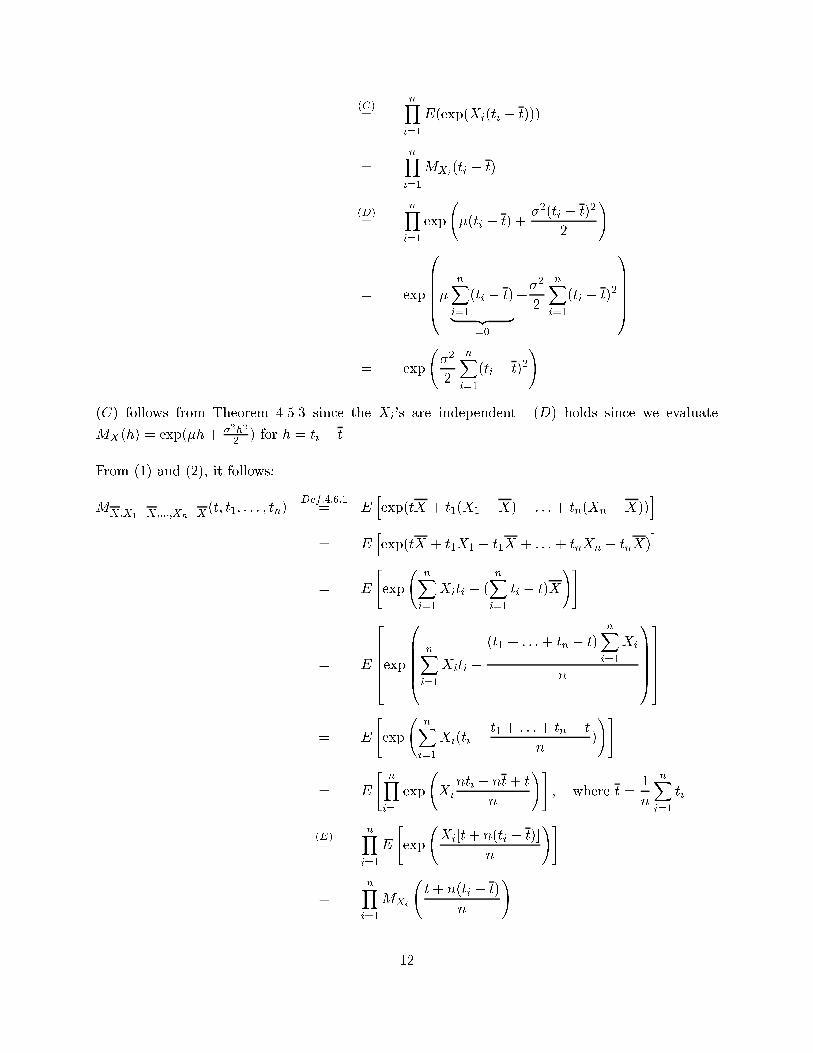
(C)=
nYi=1
E(exp(Xi(ti � t)))
=nYi=1
MXi(ti � t)
(D)=
nYi=1
exp
�(ti � t) +
�2(ti � t)2
2
!
= exp
0BBBB@�nXi=1
(ti � t)| {z }=0
+�2
2
nXi=1
(ti � t)2
1CCCCA= exp
�2
2
nXi=1
(ti � t)2
!
(C) follows from Theorem 4.5.3 since the Xi's are independent. (D) holds since we evaluate
MX(h) = exp(�h+ �2h2
2 ) for h = ti � t.
From (1) and (2), it follows:
MX;X1�X;:::;Xn�X(t; t1; : : : ; tn)
Def:4:6:1= E
hexp(tX + t1(X1 �X) + : : :+ tn(Xn �X))
i= E
hexp(tX + t1X1 � t1X + : : : + tnXn � tnX)
i= E
"exp
nXi=1
Xiti � (nXi=1
ti � t)X
!#
= E
266664exp0BBBB@
nXi=1
Xiti �(t1 + : : :+ tn � t)
nXi=1
Xi
n
1CCCCA377775
= E
"exp
nXi=1
Xi(ti �t1 + : : : + tn � t
n)
!#
= E
"nYi=1
exp
Xi
nti � nt+ t
n
!#; where t =
1
n
nXi=1
ti
(E)=
nYi=1
E
"exp
Xi[t+ n(ti � t)]
n
!#
=nYi=1
MXi
t+ n(ti � t)
n
!
12
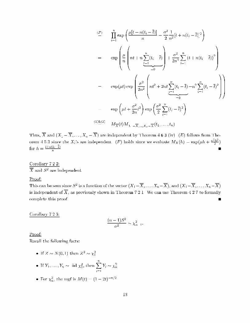
(F )=
nYi=1
exp
�[t+ n(ti � t)]
n+�2
2
1
n2[t+ n(ti � t)]2
!
= exp
0BBBB@�n0BBBB@nt+ n
nXi=1
(ti � t)| {z }=0
1CCCCA+�2
2n2
nXi=1
(t+ n(ti � t))2
1CCCCA
= exp(�t) exp
0BBBB@ �2
2n2
0BBBB@nt2 + 2ntnXi=1
(ti � t)| {z }=0
+n2nXi=1
(ti � t)2
1CCCCA1CCCCA
= exp
�t+
�2
2nt2
!exp
�2
2
nXi=1
(ti � t)2
!
(1)&(2)= M
X(t)M
X1�X;:::;Xn�X(t1; : : : ; tn)
Thus, X and (X1�X; : : : ;Xn�X) are independent by Theorem 4.6.3 (iv). (E) follows from The-
orem 4.5.3 since the Xi's are independent. (F ) holds since we evaluate MX(h) = exp(�h + �2h2
2 )
for h =t+n(ti�t)
n.
Corollary 7.2.2:
X and S2 are independent.
Proof:
This can be seen since S2 is a function of the vector (X1�X; : : : ;Xn�X), and (X1�X; : : : ;Xn�X)
is independent of X , as previously shown in Theorem 7.2.1. We can use Theorem 4.2.7 to formally
complete this proof.
Corollary 7.2.3:
(n� 1)S2
�2� �2n�1:
Proof:
Recall the following facts:
� If Z � N(0; 1) then Z2 � �21.
� If Y1; : : : ; Yn � iid �21, thennXi=1
Yi � �2n.
� For �2n, the mgf is M(t) = (1� 2t)�n=2.
13
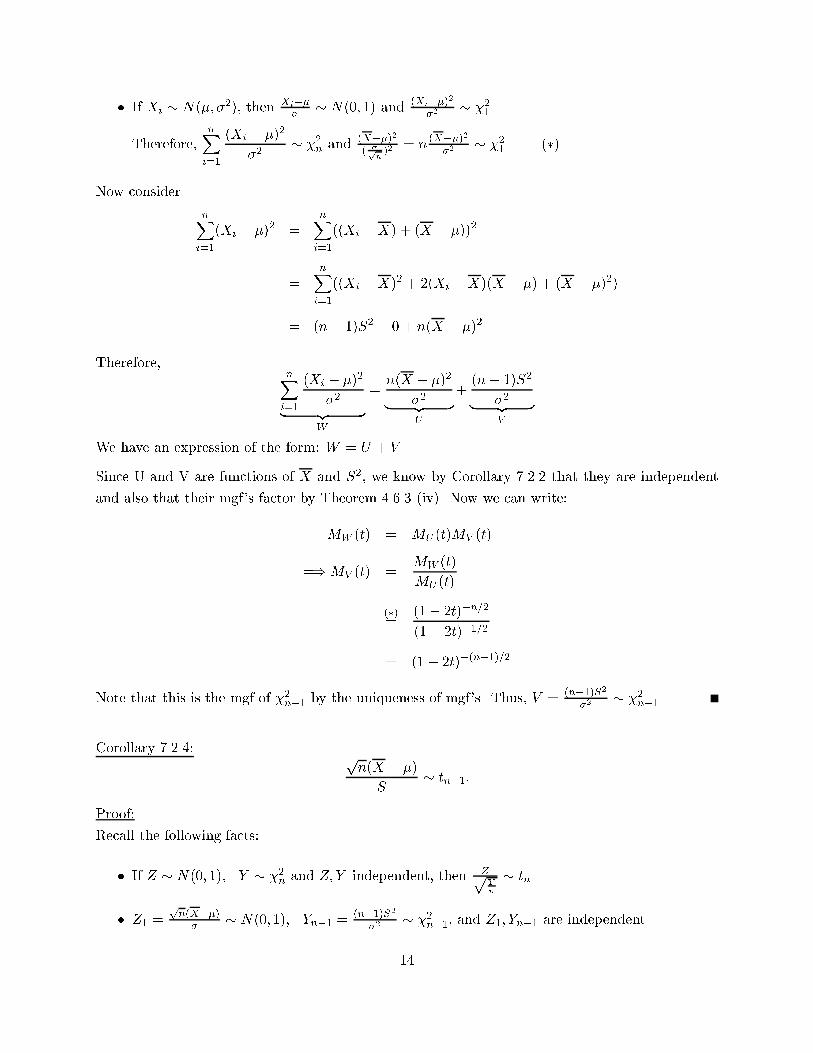
� If Xi � N(�; �2), then Xi���
� N(0; 1) and(Xi��)2
�2� �21.
Therefore,nXi=1
(Xi � �)2
�2� �2n and
(X��)2( �p
n)2
= n(X��)2
�2� �21. (�)
Now consider
nXi=1
(Xi � �)2 =nXi=1
((Xi �X) + (X � �))2
=nXi=1
((Xi �X)2 + 2(Xi �X)(X � �) + (X � �)2)
= (n� 1)S2 + 0 + n(X � �)2
Therefore,nXi=1
(Xi � �)2
�2| {z }W
=n(X � �)2
�2| {z }U
+(n� 1)S2
�2| {z }V
We have an expression of the form: W = U + V
Since U and V are functions of X and S2, we know by Corollary 7.2.2 that they are independent
and also that their mgf's factor by Theorem 4.6.3 (iv). Now we can write:
MW (t) = MU (t)MV (t)
=)MV (t) =MW (t)
MU (t)
(�)=
(1� 2t)�n=2
(1� 2t)�1=2
= (1� 2t)�(n�1)=2
Note that this is the mgf of �2n�1 by the uniqueness of mgf's. Thus, V =
(n�1)S2�2
� �2n�1.
Corollary 7.2.4: pn(X � �)
S� tn�1:
Proof:
Recall the following facts:
� If Z � N(0; 1); Y � �2n and Z; Y independent, then ZpY
n
� tn.
� Z1 =pn(X��)�
� N(0; 1); Yn�1 =(n�1)S2
�2� �2
n�1, and Z1; Yn�1 are independent.
14
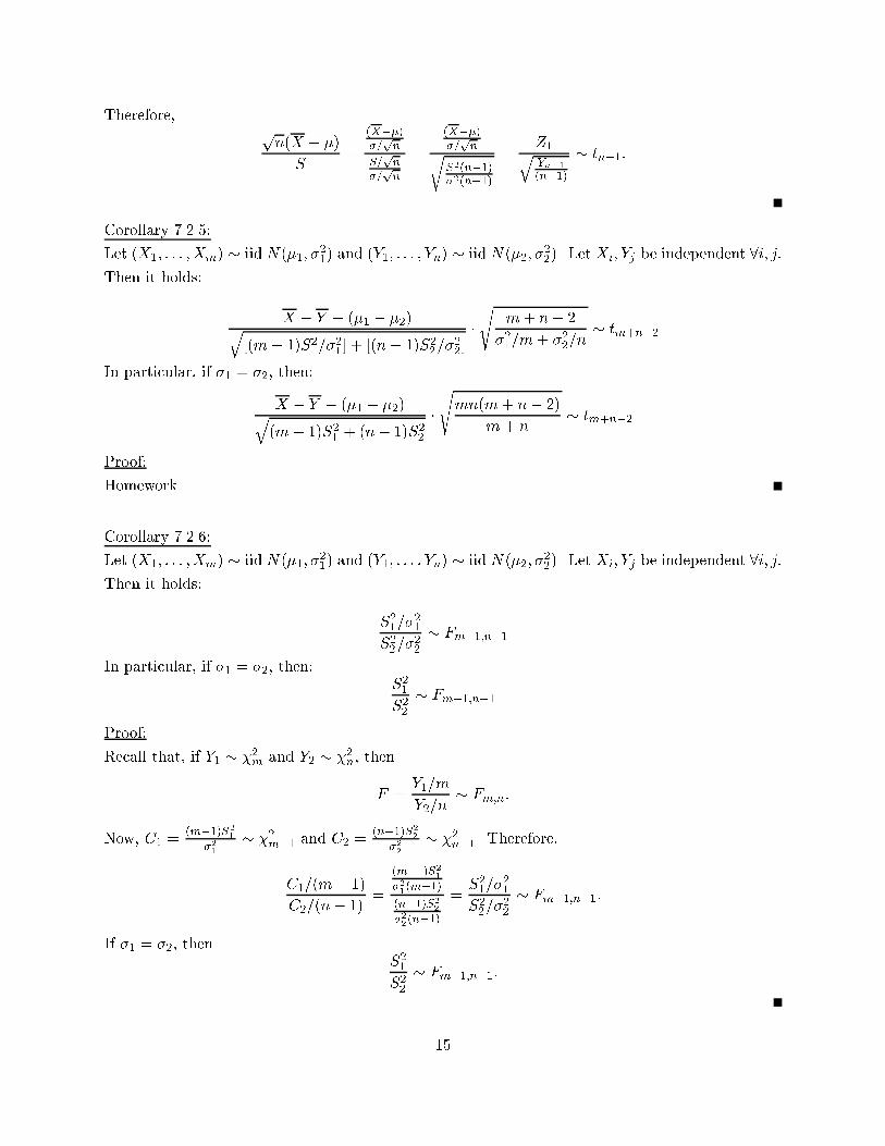
Therefore,pn(X � �)
S=
(X��)�=pn
S=pn
�=pn
=
(X��)�=pnr
S2(n�1)�2(n�1)
=Z1qYn�1
(n�1)
� tn�1:
Corollary 7.2.5:
Let (X1; : : : ;Xm) � iid N(�1; �21) and (Y1; : : : ; Yn) � iid N(�2; �
22). Let Xi; Yj be independent 8i; j:
Then it holds:
X � Y � (�1 � �2)q[(m� 1)S21=�
21 ] + [(n� 1)S22=�
22 ]�s
m+ n� 2
�21=m+ �22=n� tm+n�2
In particular, if �1 = �2, then:
X � Y � (�1 � �2)q(m� 1)S21 + (n� 1)S22
�
smn(m+ n� 2)
m+ n� tm+n�2
Proof:
Homework.
Corollary 7.2.6:
Let (X1; : : : ;Xm) � iid N(�1; �21) and (Y1; : : : ; Yn) � iid N(�2; �
22). Let Xi; Yj be independent 8i; j:
Then it holds:
S21=�21
S22=�22
� Fm�1;n�1
In particular, if �1 = �2, then:S21
S22� Fm�1;n�1
Proof:
Recall that, if Y1 � �2m and Y2 � �2n, then
F =Y1=m
Y2=n� Fm;n:
Now, C1 =(m�1)S21
�21
� �2m�1 and C2 =(n�1)S22
�22
� �2n�1. Therefore,
C1=(m� 1)
C2=(n� 1)=
(m�1)S21�21(m�1)
(n�1)S22�22(n�1)
=S21=�
21
S22=�22
� Fm�1;n�1:
If �1 = �2, thenS21
S22� Fm�1;n�1:
15
Stat 6720 Mathematical Statistics II Spring Semester 2000
Lecture 6: Monday 1/24/2000
Scribe: J�urgen Symanzik
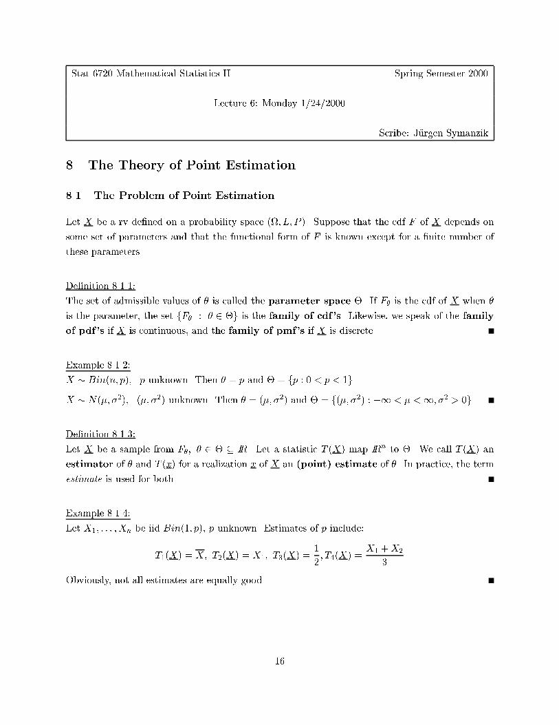
8 The Theory of Point Estimation
8.1 The Problem of Point Estimation
Let X be a rv de�ned on a probability space (; L; P ). Suppose that the cdf F of X depends on
some set of parameters and that the functional form of F is known except for a �nite number of
these parameters.
De�nition 8.1.1:
The set of admissible values of � is called the parameter space �. If F� is the cdf of X when �
is the parameter, the set fF� : � 2 �g is the family of cdf's. Likewise, we speak of the family
of pdf's if X is continuous, and the family of pmf's if X is discrete.
Example 8.1.2:
X � Bin(n; p); p unknown. Then � = p and � = fp : 0 < p < 1g.
X � N(�; �2); (�; �2) unknown. Then � = (�; �2) and � = f(�; �2) : �1 < � <1; �2 > 0g.
De�nition 8.1.3:
Let X be a sample from F�; � 2 � � IR. Let a statistic T (X) map IRn to �. We call T (X) an
estimator of � and T (x) for a realization x of X an (point) estimate of �. In practice, the term
estimate is used for both.
Example 8.1.4:
Let X1; : : : ; Xn be iid Bin(1; p), p unknown. Estimates of p include:
T1(X) = X; T2(X) = X1; T3(X) =1
2; T4(X) =
X1 +X2
3
Obviously, not all estimates are equally good.
16
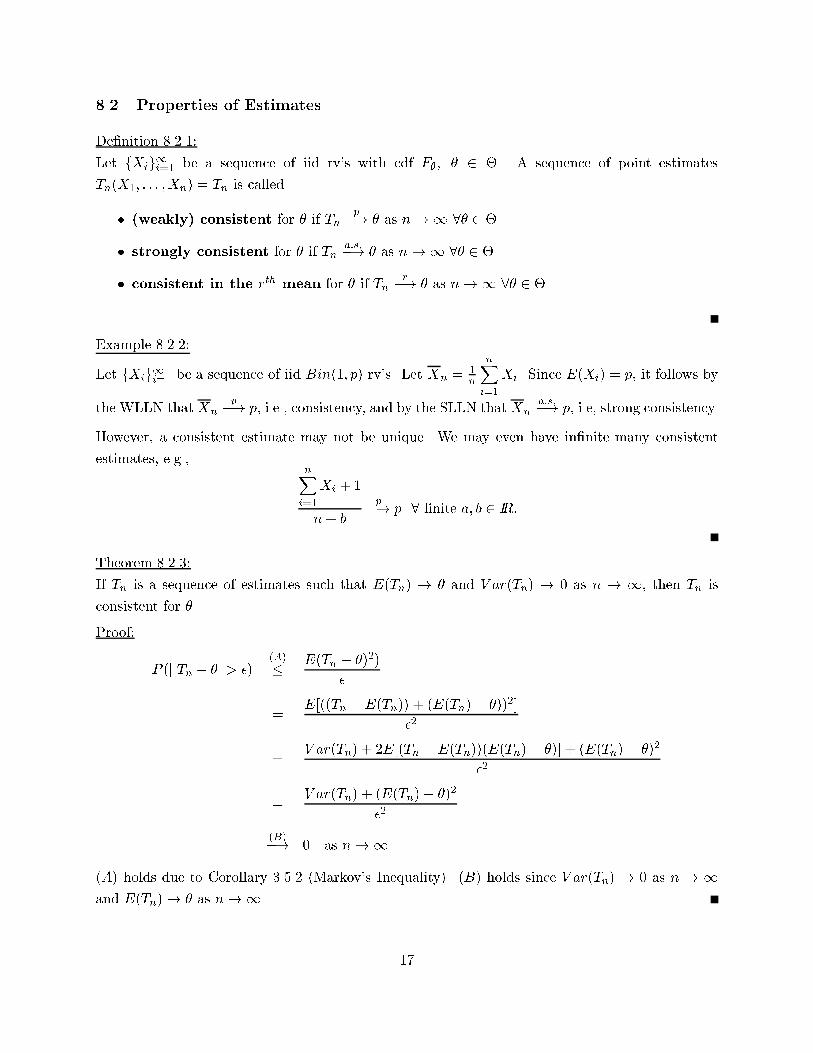
8.2 Properties of Estimates
De�nition 8.2.1:
Let fXig1i=1 be a sequence of iid rv's with cdf F�; � 2 �. A sequence of point estimates
Tn(X1; : : : ; Xn) = Tn is called
� (weakly) consistent for � if Tnp�! � as n!1 8� 2 �
� strongly consistent for � if Tna:s:�! � as n!1 8� 2 �
� consistent in the rth mean for � if Tnr�! � as n!1 8� 2 �
Example 8.2.2:
Let fXig1i=1 be a sequence of iid Bin(1; p) rv's. Let Xn =1n
nXi=1
Xi. Since E(Xi) = p, it follows by
the WLLN that Xn
p�! p, i.e., consistency, and by the SLLN that Xn
a:s:�! p, i.e, strong consistency.
However, a consistent estimate may not be unique. We may even have in�nite many consistent
estimates, e.g.,nXi=1
Xi + 1
n+ b
p�! p 8 �nite a; b 2 IR:
Theorem 8.2.3:
If Tn is a sequence of estimates such that E(Tn) ! � and V ar(Tn) ! 0 as n ! 1, then Tn is
consistent for �.
Proof:
P (j Tn � � j> �)(A)
� E(Tn � �)2)
�
=E[((Tn �E(Tn)) + (E(Tn)� �))2]
�2
=V ar(Tn) + 2E[(Tn �E(Tn))(E(Tn)� �)] + (E(Tn)� �)2
�2
=V ar(Tn) + (E(Tn)� �)2
�2
(B)�! 0 as n!1
(A) holds due to Corollary 3.5.2 (Markov's Inequality). (B) holds since V ar(Tn) ! 0 as n ! 1and E(Tn)! � as n!1.
17
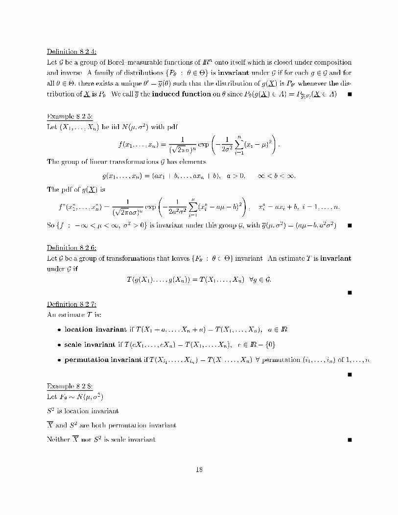
De�nition 8.2.4:
Let G be a group of Borel{measurable functions of IRn onto itself which is closed under composition
and inverse. A family of distributions fP� : � 2 �g is invariant under G if for each g 2 G and for
all � 2 �, there exists a unique �0 = g(�) such that the distribution of g(X) is P�0 whenever the dis-
tribution of X is P�. We call g the induced function on � since P�(g(X) 2 A) = Pg(�)(X 2 A).
Example 8.2.5:
Let (X1; : : : ;Xn) be iid N(�; �2) with pdf
f(x1; : : : ; xn) =1
(p2��)n
exp
� 1
2�2
nXi=1
(xi � �)2!:
The group of linear transformations G has elements
g(x1; : : : ; xn) = (ax1 + b; : : : ; axn + b); a > 0; �1 < b <1:
The pdf of g(X) is
f�(x�1; : : : ; x�n) =
1
(p2�a�)n
exp
� 1
2a2�2
nXi=1
(x�i � a�� b)2!; x�i = axi + b; i = 1; : : : ; n:
So ff : �1 < � <1; �2 > 0g is invariant under this group G, with g(�; �2) = (a�+b; a2�2).
De�nition 8.2.6:
Let G be a group of transformations that leaves fF� : � 2 �g invariant. An estimate T is invariant
under G if
T (g(X1); : : : ; g(Xn)) = T (X1; : : : ;Xn) 8g 2 G:
De�nition 8.2.7:
An estimate T is:
� location invariant if T (X1 + a; : : : ;Xn + a) = T (X1; : : : ; Xn); a 2 IR
� scale invariant if T (cX1; : : : ; cXn) = T (X1; : : : ;Xn); c 2 IR� f0g
� permutation invariant if T (Xi1 ; : : : ; Xin) = T (X1; : : : ;Xn) 8 permutation (i1; : : : ; in) of 1; : : : ; n
Example 8.2.8:
Let F� � N(�; �2).
S2 is location invariant.
X and S2 are both permutation invariant.
Neither X nor S2 is scale invariant.
18
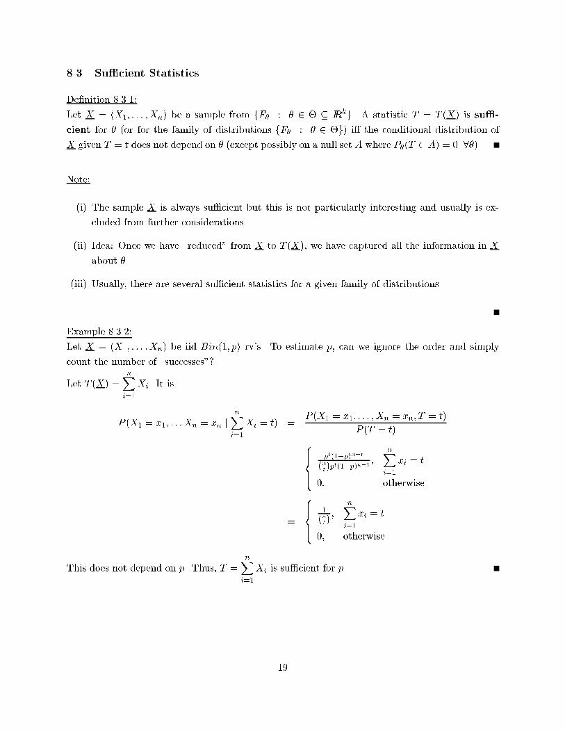
8.3 Su�cient Statistics
De�nition 8.3.1:
Let X = (X1; : : : ;Xn) be a sample from fF� : � 2 � � IRkg. A statistic T = T (X) is su�-
cient for � (or for the family of distributions fF� : � 2 �g) i� the conditional distribution of
X given T = t does not depend on � (except possibly on a null set A where P�(T 2 A) = 0 8�).
Note:
(i) The sample X is always su�cient but this is not particularly interesting and usually is ex-
cluded from further considerations.
(ii) Idea: Once we have \reduced" from X to T (X), we have captured all the information in X
about �.
(iii) Usually, there are several su�cient statistics for a given family of distributions
Example 8.3.2:
Let X = (X1; : : : ;Xn) be iid Bin(1; p) rv's. To estimate p, can we ignore the order and simply
count the number of \successes"?
Let T (X) =nXi=1
Xi. It is
P (X1 = x1; : : : Xn = xn jnXi=1
Xi = t) =P (X1 = x1; : : : ;Xn = xn; T = t)
P (T = t)
=
8>><>>:pt(1�p)n�t
(nt)pt(1�p)n�t ;
nXi=1
xi = t
0; otherwise
=
8>><>>:1
(nt);
nXi=1
xi = t
0; otherwise
This does not depend on p. Thus, T =nXi=1
Xi is su�cient for p.
19
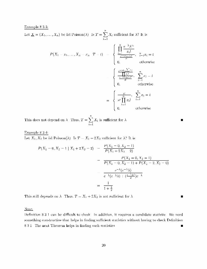
Example 8.3.3:
Let X = (X1; : : : ;Xn) be iid Poisson(�). Is T =nXi=1
Xi su�cient for �? It is
P (X1 = x1; : : : ;Xn = xn j T = t) =
8>>>><>>>>:
nYi=1
e���xi
xi!e�n�(n�)t
t!
; n
i=1xi = t
0; otherwise
=
8>>><>>>:e�n��
PxiQ
xi!
e�n�(n�)tt!
;
nXi=1
xi = t
0; otherwise
=
8>>>><>>>>:t!
nt
nYi=1
xi!
;
nXi=1
xi = t
0; otherwise
This does not depend on �. Thus, T =nXi=1
Xi is su�cient for �.
Example 8.3.4:
Let X1; X2 be iid Poisson(�). Is T = X1 + 2X2 su�cient for �? It is
P (X1 = 0;X2 = 1 j X1 + 2X2 = 2) =P (X1 = 0;X2 = 1)
P (X1 + 2X2 = 2)
=P (X1 = 0; X2 = 1)
P (X1 = 0;X2 = 1) + P (X1 = 2;X2 = 0)
=e��(e���)
e��(e���) + ( e���2
2 )e��
=1
1 + �
2
This still depends on �. Thus, T = X1 + 2X2 is not su�cient for �.
Note:
De�nition 8.3.1 can be di�cult to check. In addition, it requires a candidate statistic. We need
something constructive that helps in �nding su�cient statistics without having to check De�nition
8.3.1. The next Theorem helps in �nding such statistics.
20
Stat 6720 Mathematical Statistics II Spring Semester 2000
Lecture 7: Wednesday 1/26/2000
Scribe: J�urgen Symanzik
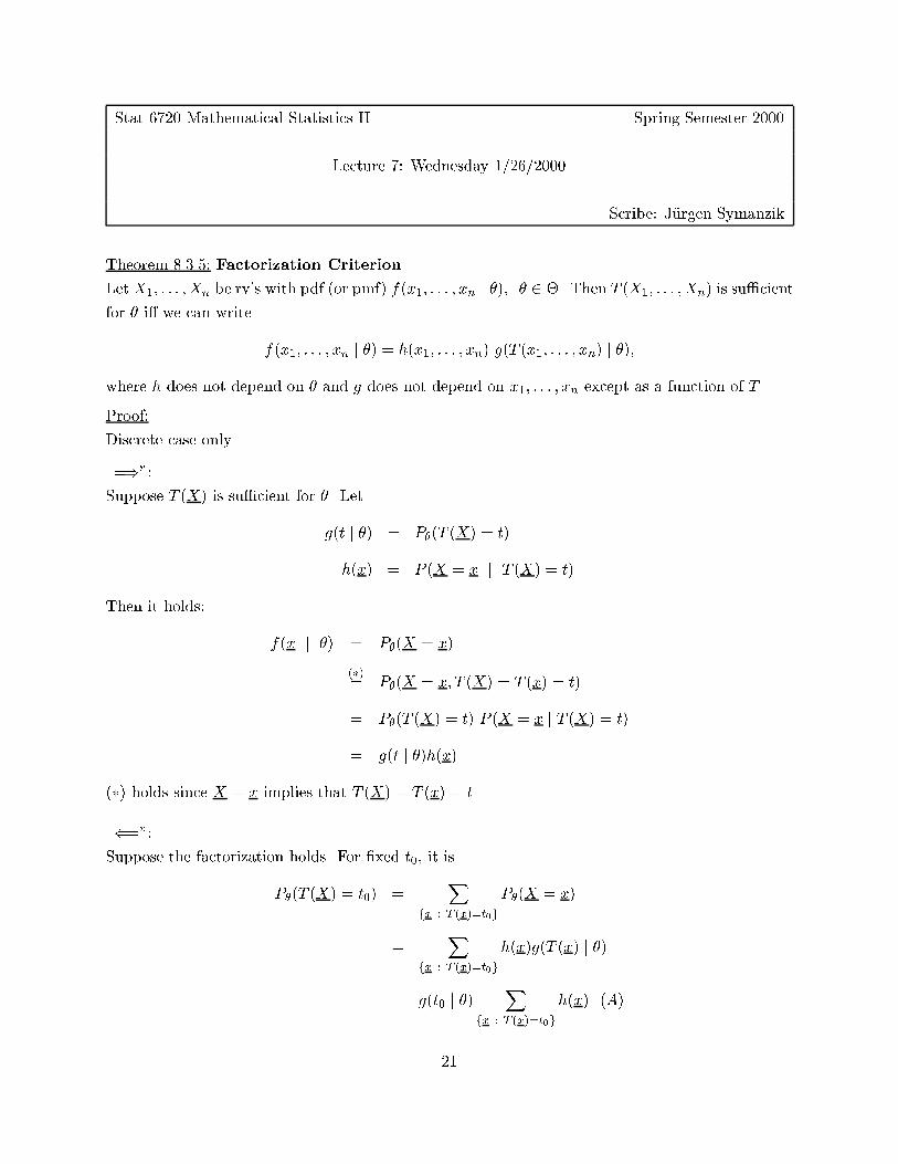
Theorem 8.3.5: Factorization Criterion
Let X1; : : : ; Xn be rv's with pdf (or pmf) f(x1; : : : ; xn j �); � 2 �. Then T (X1; : : : ;Xn) is su�cient
for � i� we can write
f(x1; : : : ; xn j �) = h(x1; : : : ; xn) g(T (x1; : : : ; xn) j �);
where h does not depend on � and g does not depend on x1; : : : ; xn except as a function of T .
Proof:
Discrete case only.
\=)":
Suppose T (X) is su�cient for �. Let
g(t j �) = P�(T (X) = t)
h(x) = P (X = x j T (X) = t)
Then it holds:
f(x j �) = P�(X = x)
(�)= P�(X = x; T (X) = T (x) = t)
= P�(T (X) = t) P (X = x j T (X) = t)
= g(t j �)h(x)
(�) holds since X = x implies that T (X) = T (x) = t.
\(=":Suppose the factorization holds. For �xed t0, it is
P�(T (X) = t0) =X
fx : T (x)=t0gP�(X = x)
=X
fx : T (x)=t0gh(x)g(T (x) j �)
= g(t0 j �)X
fx : T (x)=t0gh(x) (A)
21
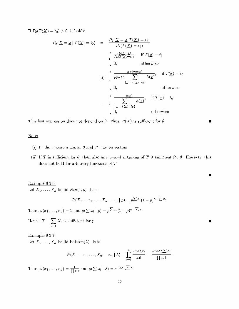
If P�(T (X) = t0) > 0, it holds:
P�(X = x j T (X) = t0) =P�(X = x; T (X) = t0)
P�(T (X) = t0)
=
8<:P�(X=x)
P�(T (X)=t0); if T (x) = t0
0; otherwise
(A)=
8>><>>:g(t0j�)h(x)
g(t0j�)X
fx : T (x)=t0gh(x)
; if T (x) = t0
0; otherwise
=
8>><>>:h(x)X
fx : T (x)=t0gh(x)
; if T (x) = t0
0; otherwise
This last expression does not depend on �. Thus, T (X) is su�cient for �.
Note:
(i) In the Theorem above, � and T may be vectors.
(ii) If T is su�cient for �, then also any 1{to{1 mapping of T is su�cient for �. However, this
does not hold for arbitrary functions of T .
Example 8.3.6:
Let X1; : : : ; Xn be iid Bin(1; p). It is
P (X1 = x1; : : : ;Xn = xn j p) = pP
xi(1� p)n�P
xi :
Thus, h(x1; : : : ; xn) = 1 and g(Pxi j p) = p
Pxi(1� p)n�
Pxi .
Hence, T =nXi=1
Xi is su�cient for p.
Example 8.3.7:
Let X1; : : : ; Xn be iid Poisson(�). It is
P (X1 = x1; : : : ;Xn = xn j �) =nYi=1
e���xi
xi!=e�n��
PxiQ
xi!:
Thus, h(x1; : : : ; xn) =1Qxi!
and g(Pxi j �) = e�n��
Pxi .
22
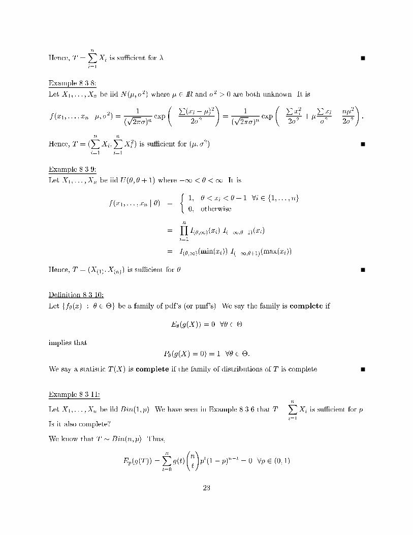
Hence, T =nXi=1
Xi is su�cient for �.
Example 8.3.8:
Let X1; : : : ; Xn be iid N(�; �2) where � 2 IR and �2 > 0 are both unknown. It is
f(x1; : : : ; xn j �; �2) =1
(p2��)n
exp
�P(xi � �)2
2�2
!=
1
(p2��)n
exp
�Px2i
2�2+ �
Pxi
�2� n�2
2�2
!:
Hence, T = (nXi=1
Xi;
nXi=1
X2i ) is su�cient for (�; �
2).
Example 8.3.9:
Let X1; : : : ; Xn be iid U(�; � + 1) where �1 < � <1. It is
f(x1; : : : ; xn j �) =
(1; � < xi < � + 1 8i 2 f1; : : : ; ng0; otherwise
=nYi=1
I(�;1)(xi) I(�1;�+1)(xi)
= I(�;1)(min(xi)) I(�1;�+1)(max(xi))
Hence, T = (X(1);X(n)) is su�cient for �.
De�nition 8.3.10:
Let ff�(x) : � 2 �g be a family of pdf's (or pmf's). We say the family is complete if
E�(g(X)) = 0 8� 2 �
implies that
P�(g(X) = 0) = 1 8� 2 �:
We say a statistic T (X) is complete if the family of distributions of T is complete.
Example 8.3.11:
Let X1; : : : ;Xn be iid Bin(1; p). We have seen in Example 8.3.6 that T =nXi=1
Xi is su�cient for p.
Is it also complete?
We know that T � Bin(n; p). Thus,
Ep(g(T )) =nXt=0
g(t)
n
t
!pt(1� p)n�t = 0 8p 2 (0; 1)
23
implies that
(1� p)nnXt=0
g(t)
n
t
!(
p
1� p)t = 0 8p 2 (0; 1) 8t:
However,nXt=0
g(t)
n
t
!(
p
1� p)t is a polynomial in p
1�p which is only equal to 0 for all p 2 (0; 1) if all
of its coe�cients are 0.
Therefore, g(t) = 0 for t = 0; 1; : : : ; n. Hence, T is complete.
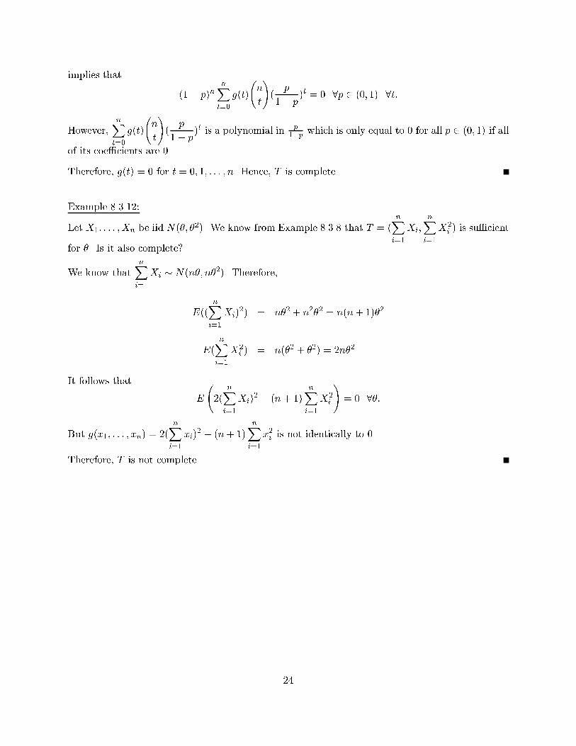
Example 8.3.12:
Let X1; : : : ;Xn be iid N(�; �2). We know from Example 8.3.8 that T = (nXi=1
Xi;
nXi=1
X2i ) is su�cient
for �. Is it also complete?
We know thatnXi=1
Xi � N(n�; n�2). Therefore,
E((nXi=1
Xi)2) = n�2 + n2�2 = n(n+ 1)�2
E(nXi=1
X2i ) = n(�2 + �2) = 2n�2
It follows that
E
2(
nXi=1
Xi)2 � (n+ 1)
nXi=1
X2i
!= 0 8�:
But g(x1; : : : ; xn) = 2(nXi=1
xi)2 � (n+ 1)
nXi=1
x2i is not identically to 0.
Therefore, T is not complete.
24
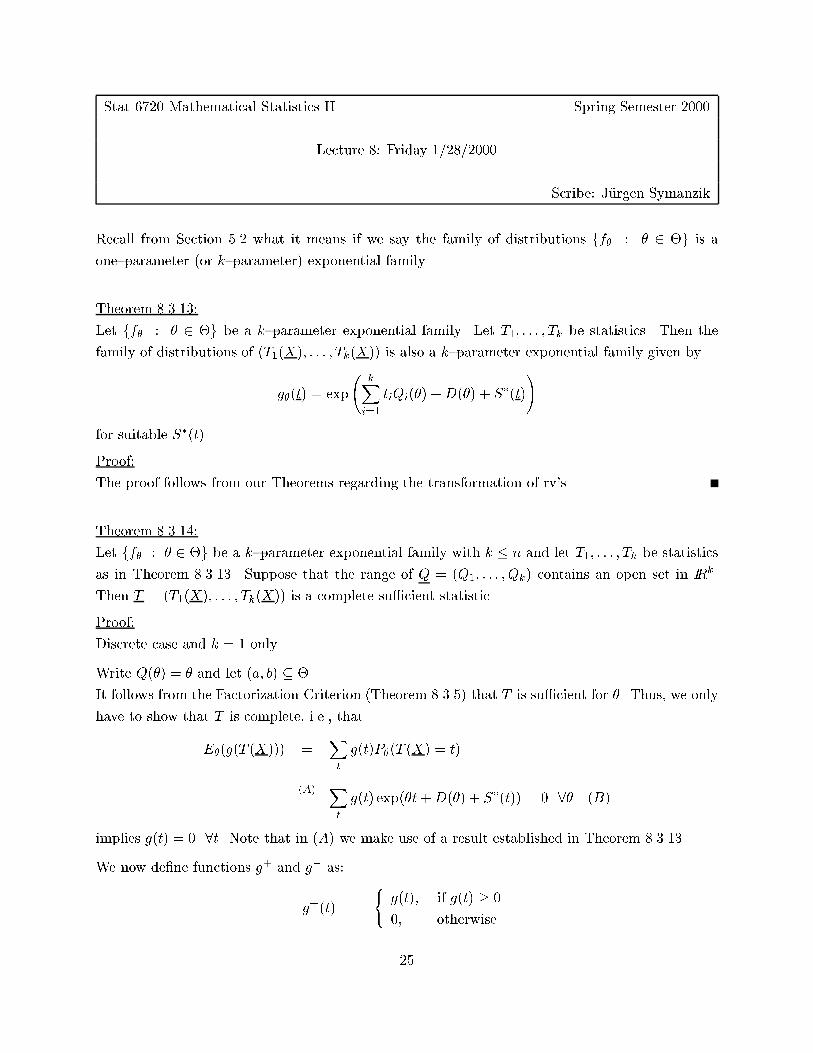
Stat 6720 Mathematical Statistics II Spring Semester 2000
Lecture 8: Friday 1/28/2000
Scribe: J�urgen Symanzik
Recall from Section 5.2 what it means if we say the family of distributions ff� : � 2 �g is a
one{parameter (or k{parameter) exponential family.
Theorem 8.3.13:
Let ff� : � 2 �g be a k{parameter exponential family. Let T1; : : : ; Tk be statistics. Then the
family of distributions of (T1(X); : : : ; Tk(X)) is also a k{parameter exponential family given by
g�(t) = exp
kXi=1
tiQi(�) +D(�) + S�(t)
!
for suitable S�(t).
Proof:
The proof follows from our Theorems regarding the transformation of rv's.
Theorem 8.3.14:
Let ff� : � 2 �g be a k{parameter exponential family with k � n and let T1; : : : ; Tk be statistics
as in Theorem 8.3.13. Suppose that the range of Q = (Q1; : : : ; Qk) contains an open set in IRk.
Then T = (T1(X); : : : ; Tk(X)) is a complete su�cient statistic.
Proof:
Discrete case and k = 1 only.
Write Q(�) = � and let (a; b) � �.
It follows from the Factorization Criterion (Theorem 8.3.5) that T is su�cient for �. Thus, we only
have to show that T is complete, i.e., that
E�(g(T (X))) =Xt
g(t)P�(T (X) = t)
(A)=
Xt
g(t) exp(�t+D(�) + S�(t)) = 0 8� (B)
implies g(t) = 0 8t. Note that in (A) we make use of a result established in Theorem 8.3.13.
We now de�ne functions g+ and g� as:
g+(t) =
(g(t); if g(t) � 0
0; otherwise
25
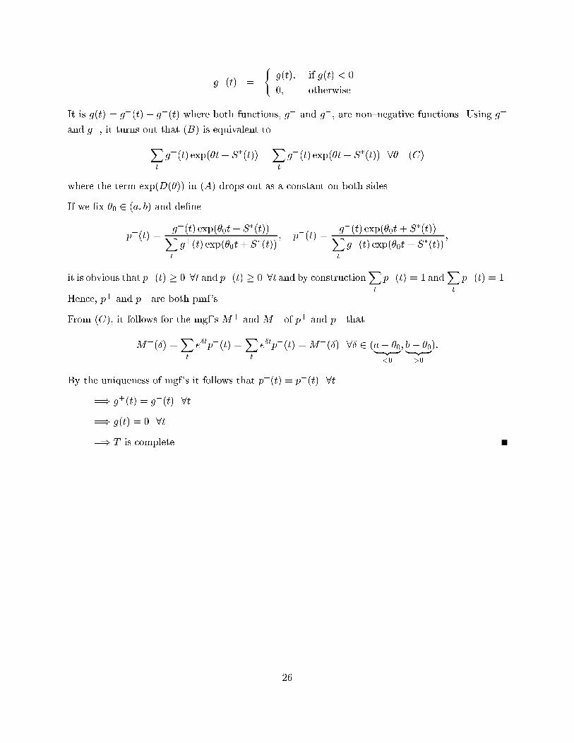
g�(t) =
(g(t); if g(t) < 0
0; otherwise
It is g(t) = g+(t)� g�(t) where both functions, g+ and g�, are non{negative functions. Using g+
and g�, it turns out that (B) is equivalent toXt
g+(t) exp(�t+ S�(t)) =Xt
g�(t) exp(�t+ S�(t)) 8� (C)
where the term exp(D(�)) in (A) drops out as a constant on both sides.
If we �x �0 2 (a; b) and de�ne
p+(t) =g+(t) exp(�0t+ S�(t))Xt
g+(t) exp(�0t+ S�(t)); p�(t) =
g�(t) exp(�0t+ S�(t))Xt
g�(t) exp(�0t+ S�(t));
it is obvious that p+(t) � 0 8t and p�(t) � 0 8t and by constructionXt
p+(t) = 1 andXt
p�(t) = 1.
Hence, p+ and p� are both pmf's.
From (C), it follows for the mgf's M+ and M� of p+ and p� that
M+(�) =Xt
e�tp+(t) =Xt
e�tp�(t) =M�(�) 8� 2 (a� �0| {z }<0
; b� �0| {z }>0
):
By the uniqueness of mgf's it follows that p+(t) = p�(t) 8t.
=) g+(t) = g�(t) 8t
=) g(t) = 0 8t
=) T is complete
26
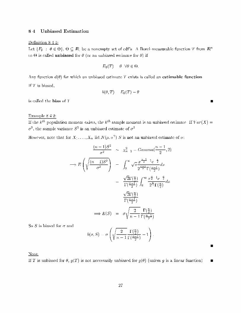
8.4 Unbiased Estimation
De�nition 8.4.1:
Let fF� : � 2 �g, � � IR, be a nonempty set of cdf's. A Borel{measurable function T from IRn
to � is called unbiased for � (or an unbiased estimate for �) if
E�(T ) = � 8� 2 �:
Any function d(�) for which an unbiased estimate T exists is called an estimable function.
If T is biased,
b(�; T ) = E�(T )� �
is called the bias of T .
Example 8.4.2:
If the kth population moment exists, the kth sample moment is an unbiased estimate. If V ar(X) =
�2, the sample variance S2 is an unbiased estimate of �2.
However, note that for X1; : : : ;Xn iid N(�; �2) S is not an unbiased estimate of �:
(n� 1)S2
�2� �2n�1 = Gamma(
n� 1
2; 2)
=) E
0@s(n� 1)S2
�2
1A =
Z 1
0
pxxn�12�1e�
x2
2n�12 �(n�12 )
dx
=
p2�(n2 )
�(n�12 )
Z 1
0
xn2�1e�
x2
2n2 �(n2 )
dx
=
p2�(n2 )
�(n�12 )
=) E(S) = �
s2
n� 1
�(n2 )
�(n�12 )
So S is biased for � and
b(�; S) = �
0@s 2
n� 1
�(n2 )
�(n�12 )� 1
1A :
Note:
If T is unbiased for �, g(T ) is not necessarily unbiased for g(�) (unless g is a linear function).
27
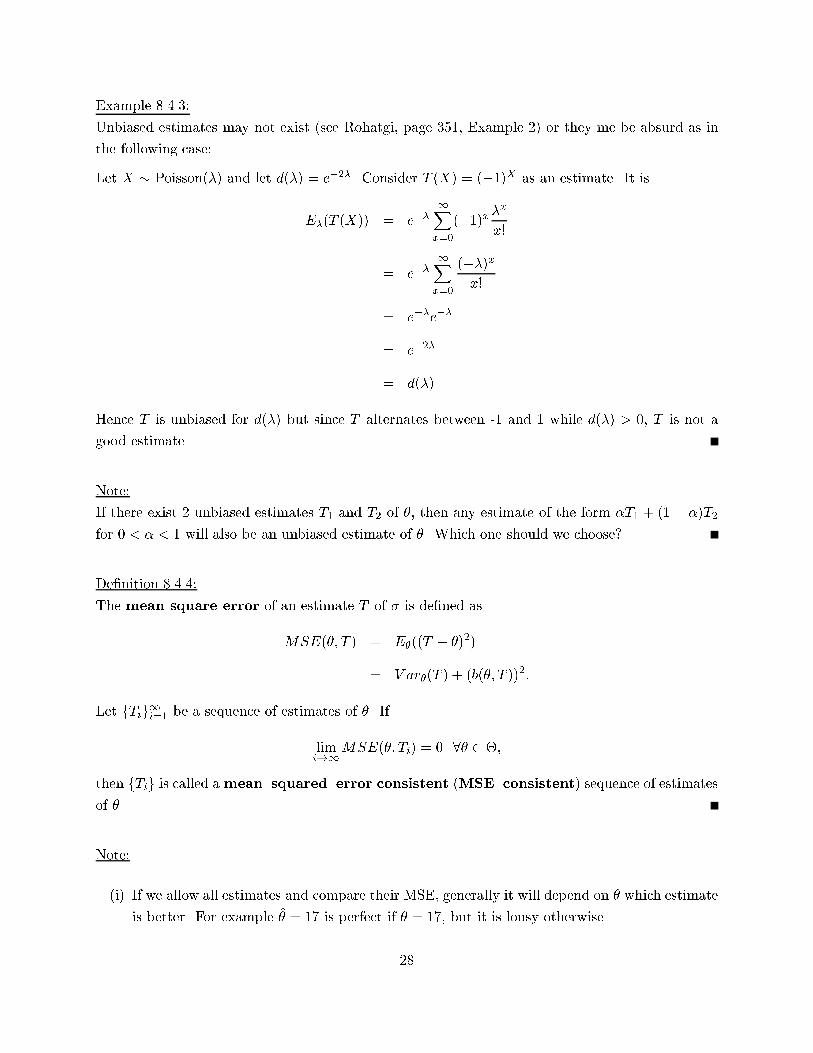
Example 8.4.3:
Unbiased estimates may not exist (see Rohatgi, page 351, Example 2) or they me be absurd as in
the following case:
Let X � Poisson(�) and let d(�) = e�2�. Consider T (X) = (�1)X as an estimate. It is
E�(T (X)) = e��1Xx=0
(�1)x�x
x!
= e��1Xx=0
(��)xx!
= e��e��
= e�2�
= d(�)
Hence T is unbiased for d(�) but since T alternates between -1 and 1 while d(�) > 0, T is not a
good estimate.
Note:
If there exist 2 unbiased estimates T1 and T2 of �, then any estimate of the form �T1 + (1 � �)T2
for 0 < � < 1 will also be an unbiased estimate of �. Which one should we choose?
De�nition 8.4.4:
The mean square error of an estimate T of � is de�ned as
MSE(�; T ) = E�((T � �)2)
= V ar�(T ) + (b(�; T ))2:
Let fTig1i=1 be a sequence of estimates of �. If
limi!1
MSE(�; Ti) = 0 8� 2 �;
then fTig is called amean{squared{error consistent (MSE{consistent) sequence of estimates
of �.
Note:
(i) If we allow all estimates and compare their MSE, generally it will depend on � which estimate
is better. For example �̂ = 17 is perfect if � = 17, but it is lousy otherwise.
28
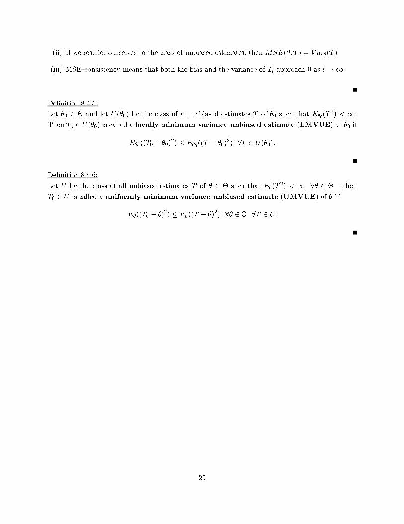
(ii) If we restrict ourselves to the class of unbiased estimates, then MSE(�; T ) = V ar�(T ).
(iii) MSE{consistency means that both the bias and the variance of Ti approach 0 as i!1.
De�nition 8.4.5:
Let �0 2 � and let U(�0) be the class of all unbiased estimates T of �0 such that E�0(T 2) < 1.
Then T0 2 U(�0) is called a locally minimum variance unbiased estimate (LMVUE) at �0 if
E�0((T0 � �0)
2) � E�0((T � �0)
2) 8T 2 U(�0):
De�nition 8.4.6:
Let U be the class of all unbiased estimates T of � 2 � such that E�(T2) < 1 8� 2 �. Then
T0 2 U is called a uniformly minimum variance unbiased estimate (UMVUE) of � if
E�((T0 � �)2) � E�((T � �)2) 8� 2 � 8T 2 U:
29
Stat 6720 Mathematical Statistics II Spring Semester 2000
Lecture 9: Monday 1/31/2000
Scribe: J�urgen Symanzik
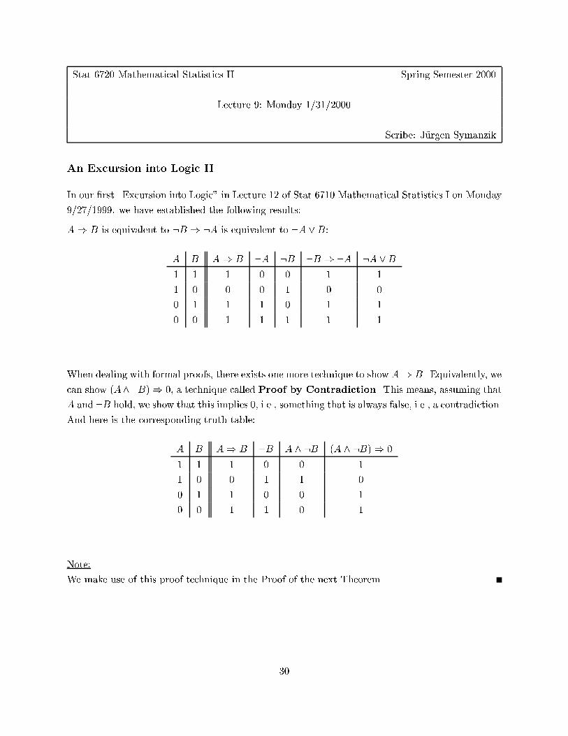
An Excursion into Logic II
In our �rst \Excursion into Logic" in Lecture 12 of Stat 6710 Mathematical Statistics I on Monday
9/27/1999, we have established the following results:
A) B is equivalent to :B ) :A is equivalent to :A _B:
A B A) B :A :B :B ) :A :A _B1 1 1 0 0 1 1
1 0 0 0 1 0 0
0 1 1 1 0 1 1
0 0 1 1 1 1 1
When dealing with formal proofs, there exists one more technique to show A) B. Equivalently, we
can show (A^:B)) 0, a technique called Proof by Contradiction. This means, assuming that
A and :B hold, we show that this implies 0, i.e., something that is always false, i.e., a contradiction.
And here is the corresponding truth table:
A B A) B :B A ^ :B (A ^ :B)) 0
1 1 1 0 0 1
1 0 0 1 1 0
0 1 1 0 0 1
0 0 1 1 0 1
Note:
We make use of this proof technique in the Proof of the next Theorem.
30
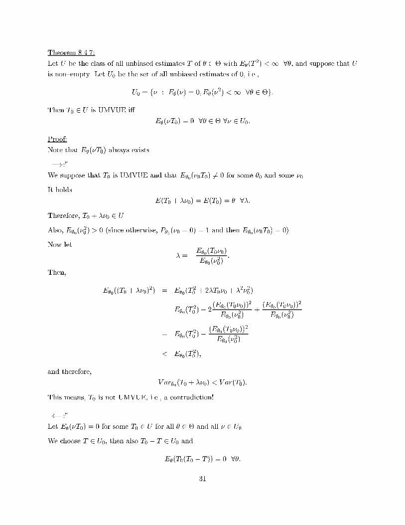
Theorem 8.4.7:
Let U be the class of all unbiased estimates T of � 2 � with E�(T2) <1 8�, and suppose that U
is non{empty. Let U0 be the set of all unbiased estimates of 0, i.e.,
U0 = f� : E�(�) = 0; E�(�2) <1 8� 2 �g:
Then T0 2 U is UMVUE i�
E�(�T0) = 0 8� 2 � 8� 2 U0:
Proof:
Note that E�(�T0) always exists.
\=):"
We suppose that T0 is UMVUE and that E�0(�0T0) 6= 0 for some �0 and some �0.
It holds
E(T0 + ��0) = E(T0) = � 8�:
Therefore, T0 + ��0 2 U .
Also, E�0(�20 ) > 0 (since otherwise, P�0(�0 = 0) = 1 and then E�0
(�0T0) = 0).
Now let
� = �E�0(T0�0)
E�0(�20)
:
Then,
E�0((T0 + ��0)
2) = E�0(T 2
0 + 2�T0�0 + �2�20 )
= E�0(T 2
0 )� 2(E�0
(T0�0))2
E�0(�20)
+(E�0
(T0�0))2
E�0(�20 )
= E�0(T 2
0 )�(E�0
(T0�0))2
E�0(�20 )
< E�0(T 2
0 );
and therefore,
V ar�0(T0 + ��0) < V ar(T0):
This means, T0 is not UMVUE, i.e., a contradiction!
\(=:"Let E�(�T0) = 0 for some T0 2 U for all � 2 � and all � 2 U0.
We choose T 2 U0, then also T0 � T 2 U0 and
E�(T0(T0 � T )) = 0 8�:
31
It follows by the Cauchy{Schwarz{Inequality, Theorem 4.5.7 (ii), that
E�(T20 ) = E�(T0T ) � (E�(T
20 ))
12 (E�(T
2))12 :
This implies
(E�(T20 ))
12 � (E�(T
2))12
and
V ar�(T0) � V ar�(T ):
32
Stat 6720 Mathematical Statistics II Spring Semester 2000
Lecture 10: Wednesday 2/2/2000
Scribe: J�urgen Symanzik
Theorem 8.4.8:
Let U be the non{empty class of unbiased estimates of � 2 � as de�ned in Theorem 8.4.7. Then
there exists at most one UMVUE T 2 U for �.
Proof:
Suppose T0; T1 2 U are both UMVUE.
Then T1 � T0 2 U0, V ar(T0) = V ar(T1), and E�(T0(T1 � T0)) = 0 8� 2 �
=) E�(T20 ) = E�(T0T1)
=) Cov(T0; T1) = E�(T0T1)�E�(T0)E�(T1)
= E�(T20 )� (E�(T0))
2
= V ar(T0)
= V ar(T1)
=) �T0T1 = 1
=) P�(aT0 + bT1 = 0) = 1 for some a; b 8� 2 �
=) � = E�(T0) = E�(� b
aT1) = E�(T1)
=) � b
a= 1
=) P�(T0 = T1) = 1 8�
Theorem 8.4.9:
(i) If an UMVUE T exists for a real function d(�), then �T is the UMVUE for �d(�); � 2 IR.
(ii) If UMVUE's T1 and T2 exist for real functions d1(�) and d2(�), respectively, then T1 + T2 is
the UMVUE for d1(�) + d2(�).
Proof:
Homework.
33
Theorem 8.4.10:
If a sample consists of n independent observations X1; : : : ;Xn from the same distribution, the
UMVUE, if it exists, is permutation invariant.
Proof:
Homework.
Theorem 8.4.11: Rao{Blackwell
Let fF� : � 2 �g be a family of cdf's, and let h be any statistic in U , where U is the non{empty
class of all unbiased estimates of � withE�(h2) <1. Let T be a su�cient statistic for fF� : � 2 �g.
Then the conditional expectation E�(h j T ) is independent of � and it is an unbiased estimate of
�. Additionally,
E�((E(h j T )� �)2) � E�((h� �)2) 8� 2 �
with equality i� h = E(h j T ).
Proof:
By Theorem 4.7.3, E�(E(h j T )) = E(h) = �.
Since X j T does not depend on � due to su�ciency, neither does E(h j T ) depend on �.
Thus, we want
E�((E(h j T ))2) � E�(h2) = E�(E(h
2 j T )):
Thus, we want
(E(h j T ))2 � E(h2 j T ):
But the Cauchy{Schwarz{Inequality gives us
(E(h j T ))2 � E(h2 j T )E(1 j T ) = E(h2 j T ):
Equality holds i�
E�((E(h j T ))2) = E�(h2)
() E�(E(h2 j T )� (E(h j T ))2) = 0
() E�(V ar(h j T )) = 0
() V ar(h j T ) = 0
() E(h2 j T ) = (E(h j T ))2
() h is a function of T and h = E(h j T ).
For the proof of the last step, see Rohatgi, page 170{171, Theorem 2, Corollary, and Proof of the
Corollary.
34
Theorem 8.4.12: Lehmann{Sche��ee
If T is a complete su�cient statistic and if there exists an unbiased estimate h of �, then E(h j T )is the (unique) UMVUE.
Proof:
Suppose that h1; h2 2 U . Then E(h1 j T ) = E(h2 j T ) = �.
Therefore,
E�(E(h1 j T )�E(h2 j T )) = 0 8� 2 �:
Since T is complete, E(h1 j T ) = E(h2 j T ).
Therefore, E(h j T ) must be the same for all h 2 U and E(h j T ) improves on all h 2 U . Therefore,E(h j T ) is UMVUE.
Note:
We can use Theorem 8.4.12 to �nd the UMVUE in two ways if we have a complete su�cient statistic
T :
(i) If we can �nd an unbiased estimate h(T ), it will be the UMVUE since E(h(T ) j T ) = h(T ).
(ii) If we have any unbiased estimate h and if we can calculate E(h j T ), then E(h j T ) willbe the UMVUE. The process of determining the UMVUE this way often is called Rao{
Blackwellization.
(iii) Even if a complete su�cient statistic does not exist, the UMVUE may still exist (see Rohatgi,
page 357{358, Example 10).
Example 8.4.13:
Let X1; : : : ; Xn be iid Bin(1; p). Then T =nXi=1
Xi is a complete su�cient statistic as seen in
Examples 8.3.6 and 8.3.11.
Since E(X1) = p, X1 is an unbiased estimate of p. However, due to part (i) of the Note above,
since X1 is not a function of T , X1 is not the UMVUE.
We can use part (ii) of the Note above to construct the UMVUE. It is
P (X1 = x j T ) =
8<:T
n; x = 1
n�Tn; x = 0
=) E(X1 j T ) = T
n= X
=) X is the UMVUE for p
35
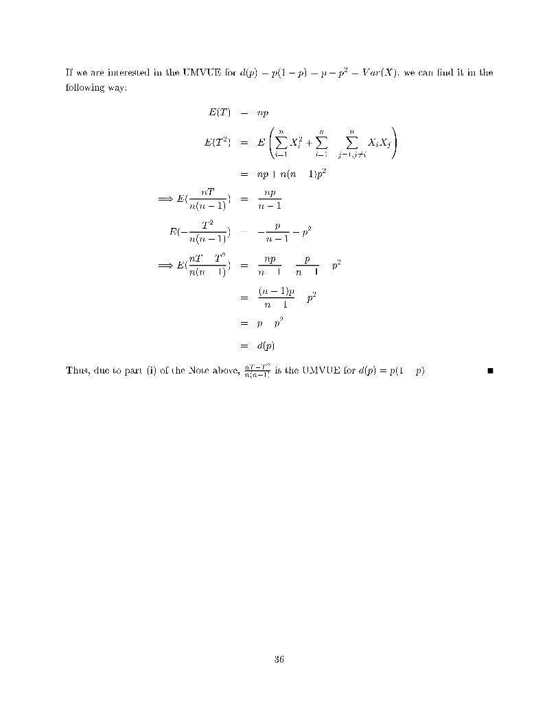
If we are interested in the UMVUE for d(p) = p(1 � p) = p� p2 = V ar(X), we can �nd it in the
following way:
E(T ) = np
E(T 2) = E
0@ nXi=1
X2i +
nXi=1
nXj=1;j 6=i
XiXj
1A= np+ n(n� 1)p2
=) E(nT
n(n� 1)) =
np
n� 1
E(� T 2
n(n� 1)) = � p
n� 1� p2
=) E(nT � T 2
n(n� 1)) =
np
n� 1� p
n� 1� p2
=(n� 1)p
n� 1� p2
= p� p2
= d(p)
Thus, due to part (i) of the Note above, nT�T 2
n(n�1) is the UMVUE for d(p) = p(1� p).
36
Stat 6720 Mathematical Statistics II Spring Semester 2000
Lecture 11: Friday 2/4/2000
Scribe: J�urgen Symanzik
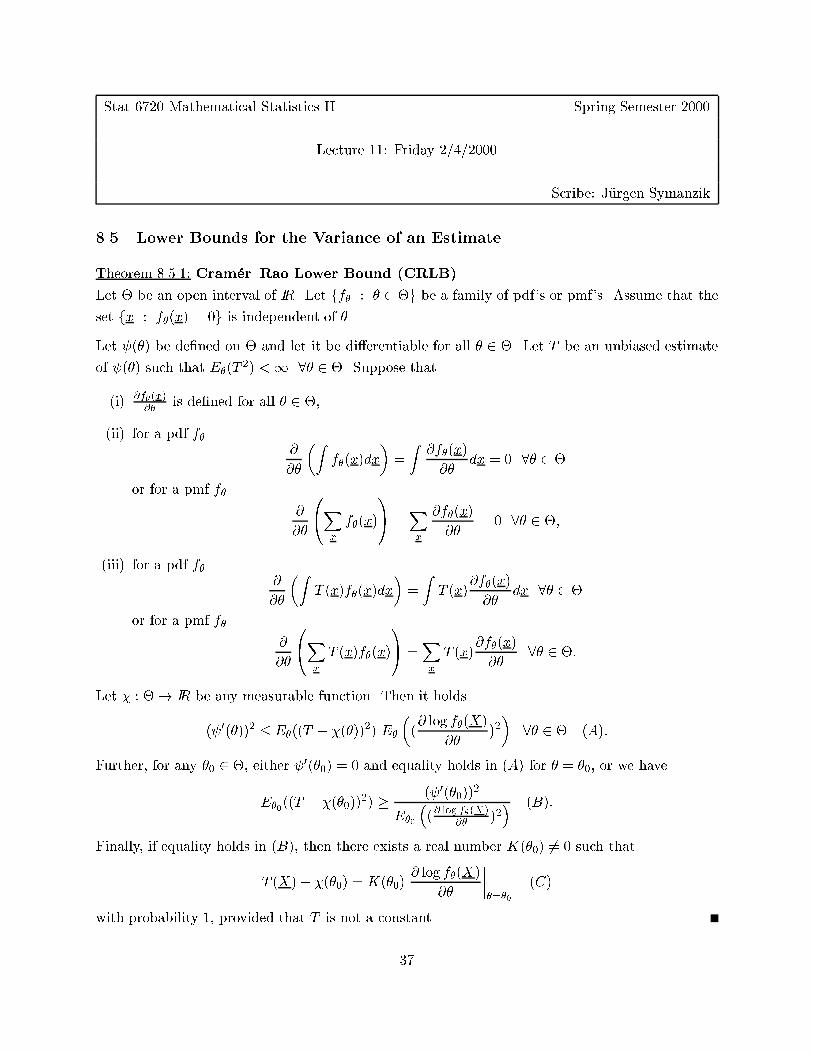
8.5 Lower Bounds for the Variance of an Estimate
Theorem 8.5.1: Cram�er{Rao Lower Bound (CRLB)
Let � be an open interval of IR. Let ff� : � 2 �g be a family of pdf's or pmf's. Assume that theset fx : f�(x) = 0g is independent of �.
Let (�) be de�ned on � and let it be di�erentiable for all � 2 �. Let T be an unbiased estimate
of (�) such that E�(T2) <1 8� 2 �. Suppose that
(i)@f�(x)@�
is de�ned for all � 2 �,
(ii) for a pdf f�@
@�
�Zf�(x)dx
�=
Z@f�(x)
@�dx = 0 8� 2 �
or for a pmf f�
@
@�
0@Xx
f�(x)
1A =Xx
@f�(x)
@�= 0 8� 2 �;
(iii) for a pdf f�@
@�
�ZT (x)f�(x)dx
�=
ZT (x)
@f�(x)
@�dx 8� 2 �
or for a pmf f�
@
@�
0@Xx
T (x)f�(x)
1A =Xx
T (x)@f�(x)
@�8� 2 �:
Let � : �! IR be any measurable function. Then it holds
( 0(�))2 � E�((T � �(�))2) E�
�(@ log f�(X)
@�)2�
8� 2 � (A):
Further, for any �0 2 �, either 0(�0) = 0 and equality holds in (A) for � = �0, or we have
E�0((T � �(�0))
2) � ( 0(�0))2
E�0
�(@ log f�(X)
@�)2� (B):
Finally, if equality holds in (B), then there exists a real number K(�0) 6= 0 such that
T (X)� �(�0) = K(�0)@ log f�(X)
@�
�����=�0
(C)
with probability 1, provided that T is not a constant.
37
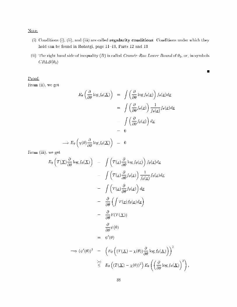
Note:
(i) Conditions (i), (ii), and (iii) are called regularity conditions. Conditions under which they
hold can be found in Rohatgi, page 11{13, Parts 12 and 13.
(ii) The right hand side of inequality (B) is called Cram�er{Rao Lower Bound of �0, or, in symbols
CRLB(�0).
Proof:
From (ii), we get
E�
�@
@�log f�(X)
�=
Z �@
@�log f�(x)
�f�(x)dx
=
Z �@
@�f�(x)
�1
f�(x)f�(x)dx
=
Z �@
@�f�(x)
�dx
= 0
=) E�
��(�)
@
@�log f�(X)
�= 0
From (iii), we get
E�
�T (X)
@
@�log f�(X)
�=
Z �T (x)
@
@�log f�(x)
�f�(x)dx
=
Z �T (x)
@
@�f�(x)
�1
f�(x)f�(x)dx
=
Z �T (x)
@
@�f�(x)
�dx
=@
@�
�ZT (x)f�(x)dx
�
=@
@�E(T (X))
=@
@� (�)
= 0(�)
=) ( 0(�))2 =
�E�
�(T (X)� �(�))
@
@�log f�(X)
��2(�)� E�
�(T (X)� �(�))2
�E�
�@
@�log f�(X)
�2!;
38
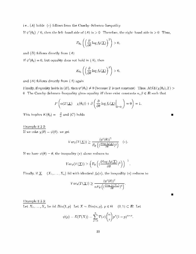
i.e., (A) holds. (�) follows from the Cauchy{Schwarz{Inequality.
If 0(�0) 6= 0, then the left{hand side of (A) is > 0. Therefore, the right{hand side is > 0. Thus,
E�0
�@
@�log f�(X)
�2!> 0;
and (B) follows directly from (A).
If 0(�0) = 0, but equality does not hold in (A), then
E�0
�@
@�log f�(X)
�2!> 0;
and (B) follows directly from (A) again.
Finally, if equality holds in (B), then 0(�0) 6= 0 (because T is not constant). Thus,MSE(�(�0); T ) >
0. The Cauchy{Schwarz{Inequality gives equality i� there exist constants �; � 2 IR such that
P
�(T (X)� �(�0)) + �
@
@�log f�(X)
�����=�0
!= 0
!= 1:
This implies K(�0) = ��
�and (C) holds.
Example 8.5.2:
If we take �(�) = (�), we get
V ar�(T (X)) � ( 0(�))2
E�
�(@ log f�(X)
@�)2� (�):
If we have (�) = �, the inequality (�) above reduces to
V ar�(T (X)) ��E�
�(@ log f�(X)
@�)2���1
:
Finally, if X = (X1; : : : ;Xn) iid with identical f�(x), the inequality (�) reduces to
V ar�(T (X)) � ( 0(�))2
nE�
�(@ log f�(X1)
@�)2� :
Example 8.5.3:
Let X1; : : : ; Xn be iid Bin(1; p). Let X � Bin(n; p), p 2 � = (0; 1) � IR. Let
(p) = E(T (X)) =nX
x=0
T (x)
n
x
!px(1� p)n�x:
39
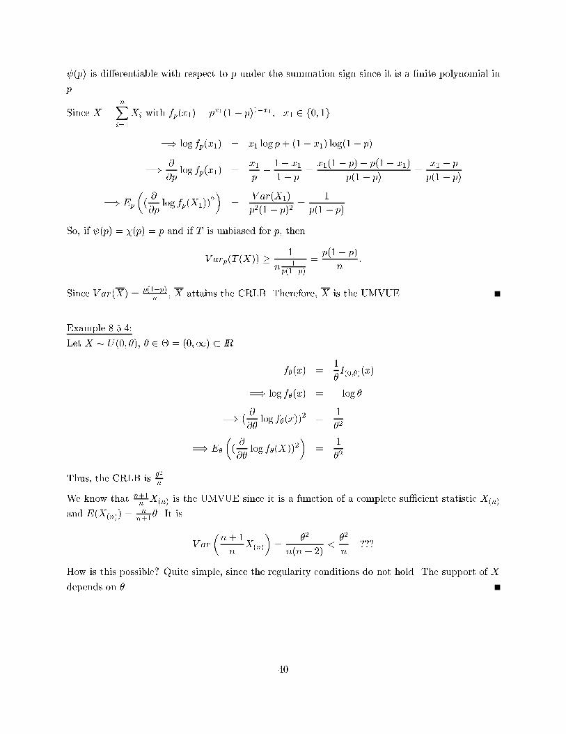
(p) is di�erentiable with respect to p under the summation sign since it is a �nite polynomial in
p.
Since X =nXi=1
Xi with fp(x1) = px1(1� p)1�x1 ; x1 2 f0; 1g
=) log fp(x1) = x1 log p+ (1� x1) log(1� p)
=) @
@plog fp(x1) =
x1
p� 1� x1
1� p=x1(1� p)� p(1� x1)
p(1� p)=
x1 � p
p(1� p)
=) Ep
�(@
@plog fp(X1))
2
�=
V ar(X1)
p2(1� p)2=
1
p(1� p)
So, if (p) = �(p) = p and if T is unbiased for p, then
V arp(T (X)) � 1
n 1p(1�p)
=p(1� p)
n:
Since V ar(X) =p(1�p)
n, X attains the CRLB. Therefore, X is the UMVUE.
Example 8.5.4:
Let X � U(0; �), � 2 � = (0;1) � IR.
f�(x) =1
�I(0;�)(x)
=) log f�(x) = � log �
=) (@
@�log f�(x))
2 =1
�2
=) E�
�(@
@�log f�(X))2
�=
1
�2
Thus, the CRLB is �2
n.
We know that n+1nX(n) is the UMVUE since it is a function of a complete su�cient statistic X(n)
and E(X(n)) =n
n+1�. It is
V ar
�n+ 1
nX(n)
�=
�2
n(n+ 2)<�2
n???
How is this possible? Quite simple, since the regularity conditions do not hold. The support of X
depends on �.
40
Stat 6720 Mathematical Statistics II Spring Semester 2000
Lecture 12: Monday 2/7/2000
Scribe: J�urgen Symanzik
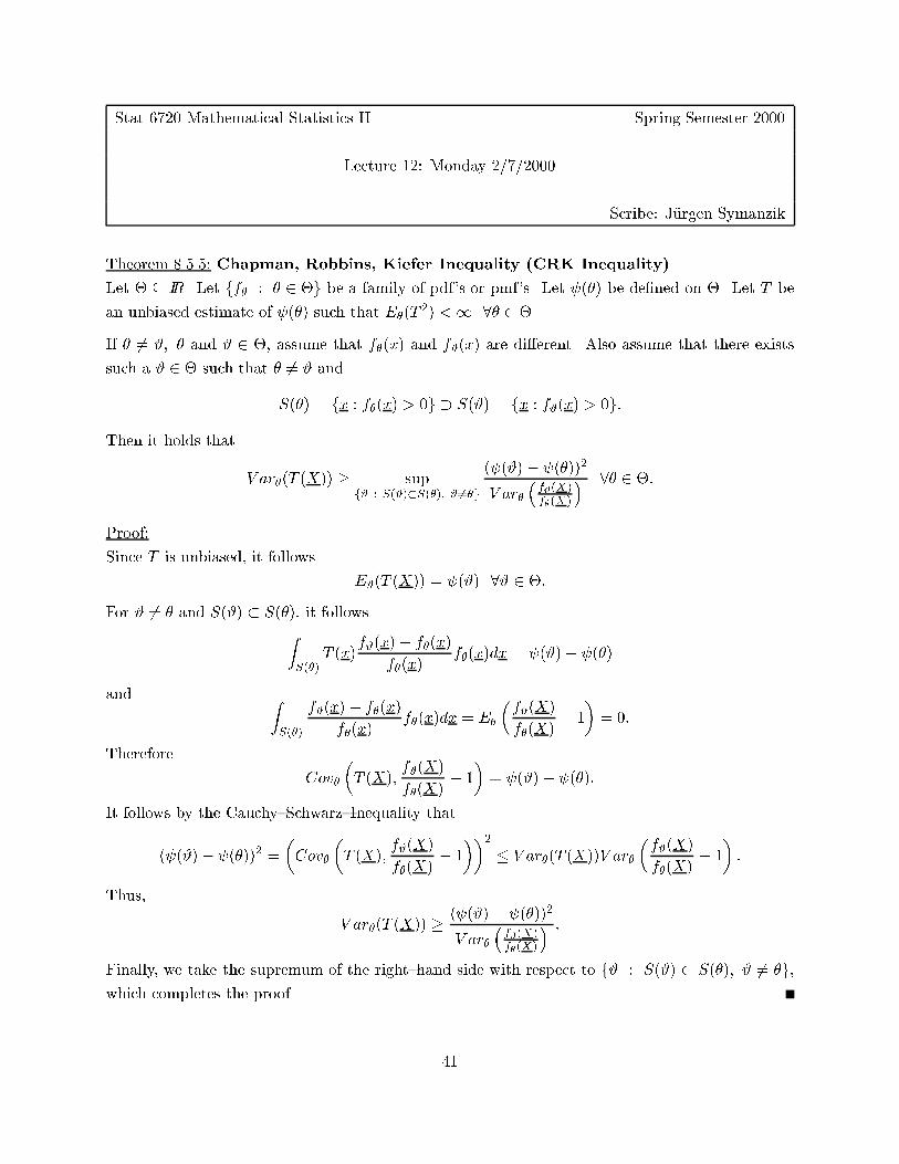
Theorem 8.5.5: Chapman, Robbins, Kiefer Inequality (CRK Inequality)
Let � � IR. Let ff� : � 2 �g be a family of pdf's or pmf's. Let (�) be de�ned on �. Let T be
an unbiased estimate of (�) such that E�(T2) <1 8� 2 �.
If � 6= #; � and # 2 �, assume that f�(x) and f#(x) are di�erent. Also assume that there exists
such a # 2 � such that � 6= # and
S(�) = fx : f�(x) > 0g � S(#) = fx : f#(x) > 0g:
Then it holds that
V ar�(T (X)) � supf# : S(#)�S(�); # 6=�g
( (#) � (�))2
V ar�
�f#(X)f�(X)
� 8� 2 �:
Proof:
Since T is unbiased, it follows
E#(T (X)) = (#) 8# 2 �:
For # 6= � and S(#) � S(�), it followsZS(�)
T (x)f#(x)� f�(x)
f�(x)f�(x)dx = (#)� (�)
and ZS(�)
f#(x)� f�(x)
f�(x)f�(x)dx = E�
�f#(X)
f�(X)� 1
�= 0:
Therefore
Cov�
�T (X);
f#(X)
f�(X)� 1
�= (#)� (�):
It follows by the Cauchy{Schwarz{Inequality that
( (#)� (�))2 =
�Cov�
�T (X);
f#(X)
f�(X)� 1
��2� V ar�(T (X))V ar�
�f#(X)
f�(X)� 1
�:
Thus,
V ar�(T (X)) � ( (#) � (�))2
V ar�
�f#(X)f�(X)
� :Finally, we take the supremum of the right{hand side with respect to f# : S(#) � S(�); # 6= �g,which completes the proof.
41
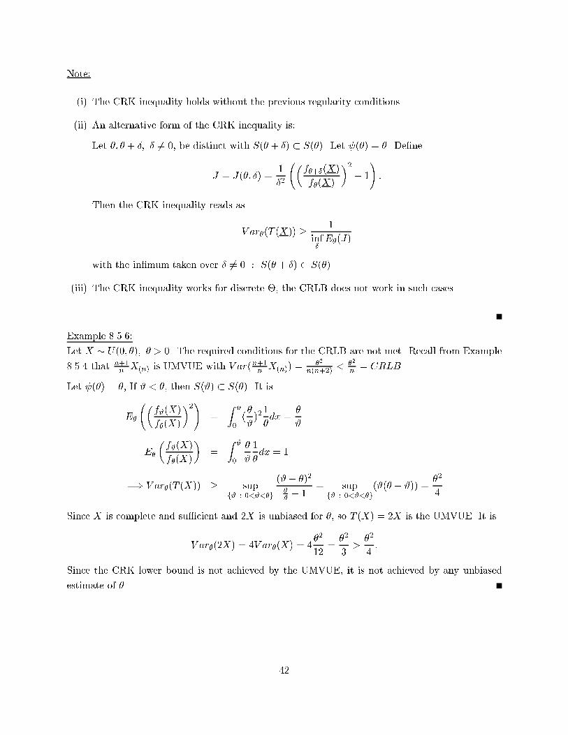
Note:
(i) The CRK inequality holds without the previous regularity conditions.
(ii) An alternative form of the CRK inequality is:
Let �; � + �; � 6= 0, be distinct with S(� + �) � S(�). Let (�) = �. De�ne
J = J(�; �) =1
�2
�f�+�(X)
f�(X)
�2� 1
!:
Then the CRK inequality reads as
V ar�(T (X)) � 1
inf�
E�(J)
with the in�mum taken over � 6= 0 : S(� + �) � S(�).
(iii) The CRK inequality works for discrete �, the CRLB does not work in such cases.
Example 8.5.6:
Let X � U(0; �); � > 0. The required conditions for the CRLB are not met. Recall from Example
8.5.4 that n+1nX(n) is UMVUE with V ar(n+1
nX(n)) =
�2
n(n+2) <�2
n= CRLB.
Let (�) = �, If # < �, then S(#) � S(�). It is
E�
�f#(X)
f�(X)
�2!=
Z#
0(�
#)21
�dx =
�
#
E�
�f#(X)
f�(X)
�=
Z#
0
�
#
1
�dx = 1
=) V ar�(T (X)) � supf# : 0<#<�g
(#� �)2
�
#� 1
= supf# : 0<#<�g
(#(� � #)) =�2
4
Since X is complete and su�cient and 2X is unbiased for �, so T (X) = 2X is the UMVUE. It is
V ar�(2X) = 4V ar�(X) = 4�2
12=�2
3>�2
4:
Since the CRK lower bound is not achieved by the UMVUE, it is not achieved by any unbiased
estimate of �.
42
Stat 6720 Mathematical Statistics II Spring Semester 2000
Lecture 13: Wednesday 2/9/2000
Scribe: J�urgen Symanzik
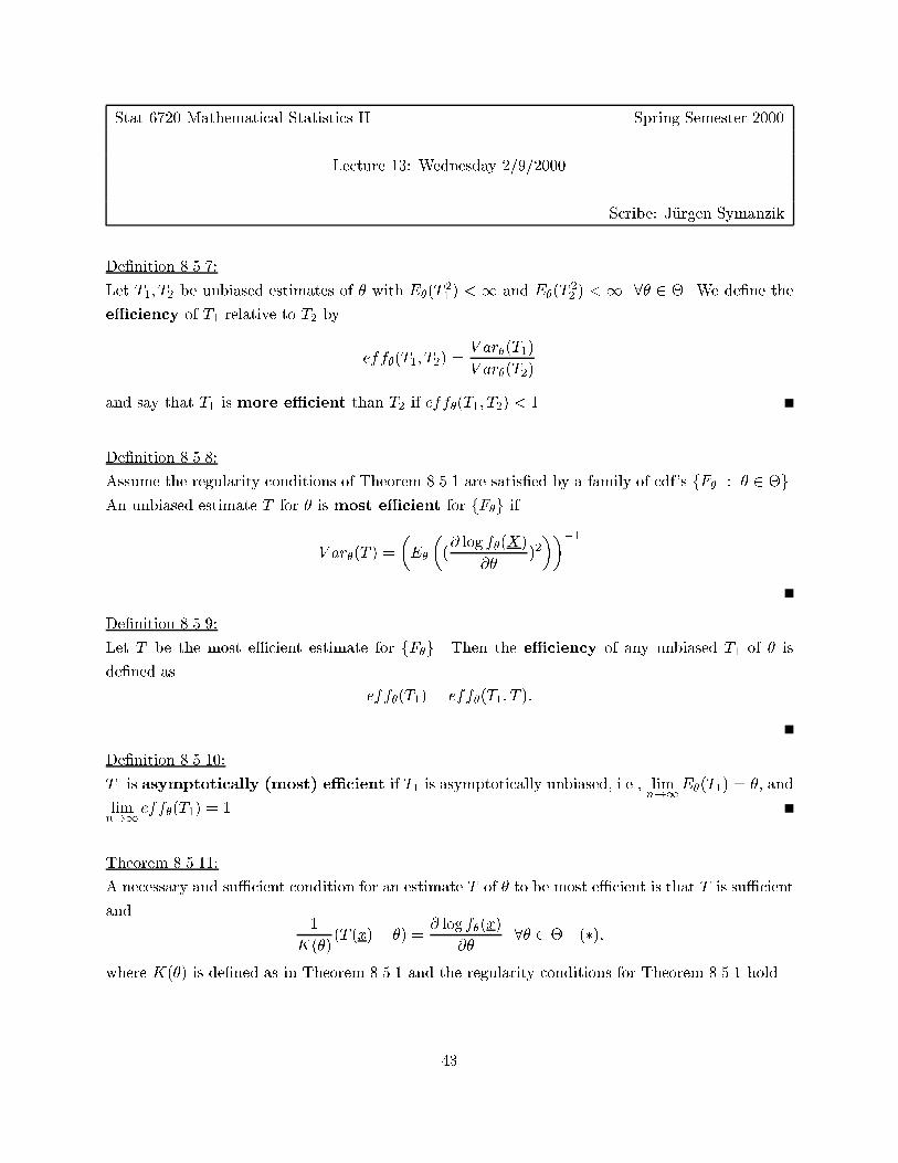
De�nition 8.5.7:
Let T1; T2 be unbiased estimates of � with E�(T21 ) < 1 and E�(T
22 ) < 1 8� 2 �. We de�ne the
e�ciency of T1 relative to T2 by
eff�(T1; T2) =V ar�(T1)
V ar�(T2)
and say that T1 is more e�cient than T2 if eff�(T1; T2) < 1.
De�nition 8.5.8:
Assume the regularity conditions of Theorem 8.5.1 are satis�ed by a family of cdf's fF� : � 2 �g.An unbiased estimate T for � is most e�cient for fF�g if
V ar�(T ) =
�E�
�(@ log f�(X)
@�)2���1
De�nition 8.5.9:
Let T be the most e�cient estimate for fF�g. Then the e�ciency of any unbiased T1 of � is
de�ned as
eff�(T1) = eff�(T1; T ):
De�nition 8.5.10:
T1 is asymptotically (most) e�cient if T1 is asymptotically unbiased, i.e., limn!1
E�(T1) = �, and
limn!1
eff�(T1) = 1.
Theorem 8.5.11:
A necessary and su�cient condition for an estimate T of � to be most e�cient is that T is su�cient
and1
K(�)(T (x)� �) =
@ log f�(x)
@�8� 2 � (�);
where K(�) is de�ned as in Theorem 8.5.1 and the regularity conditions for Theorem 8.5.1 hold.
43
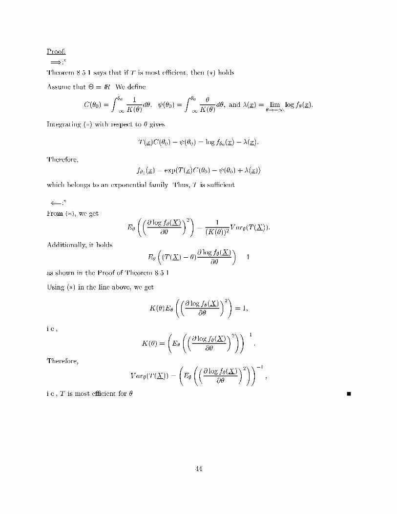
Proof:
\=):"
Theorem 8.5.1 says that if T is most e�cient, then (�) holds.
Assume that � = IR. We de�ne
C(�0) =
Z�0
�1
1
K(�)d�; (�0) =
Z�0
�1
�
K(�)d�; and �(x) = lim
�!�1log f�(x):
Integrating (�) with respect to � gives
T (x)C(�0)� (�0) = log f�0(x)� �(x):
Therefore,
f�0(x) = exp(T (x)C(�0)� (�0) + �(x))
which belongs to an exponential family. Thus, T is su�cient.
\(=:"From (�), we get
E�
�@ log f�(X)
@�
�2!=
1
(K(�))2V ar�(T (X)):
Additionally, it holds
E�
�(T (X)� �)
@ log f�(X)
@�
�= 1
as shown in the Proof of Theorem 8.5.1.
Using (�) in the line above, we get
K(�)E�
�@ log f�(X)
@�
�2!= 1;
i.e.,
K(�) =
E�
�@ log f�(X)
@�
�2!!�1:
Therefore,
V ar�(T (X)) =
E�
�@ log f�(X)
@�
�2!!�1;
i.e., T is most e�cient for �.
44
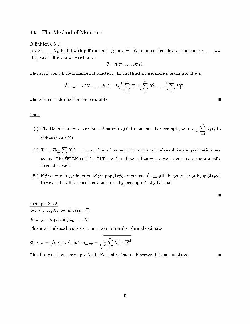
8.6 The Method of Moments
De�nition 8.6.1:
Let X1; : : : ;Xn be iid with pdf (or pmf) f�; � 2 �. We assume that �rst k moments m1; : : : ;mk
of f� exist. If � can be written as
� = h(m1; : : : ;mk);
where h is some known numerical function, the method of moments estimate of � is
�̂mom = T (X1; : : : ;Xn) = h(1
n
nXi=1
Xi;1
n
nXi=1
X2i ; : : : ;
1
n
nXi=1
Xk
i );
where h must also be Borel{measurable.
Note:
(i) The De�nition above can be estimated to joint moments. For example, we use 1n
nXi=1
XiYi to
estimate E(XY ).
(ii) Since E( 1n
nXi=1
Xj
i) = mj , method of moment estimates are unbiased for the population mo-
ments. The WLLN and the CLT say that these estimates are consistent and asymptotically
Normal as well.
(iii) If � is not a linear function of the population moments, �̂mom will, in general, not be unbiased.
However, it will be consistent and (usually) asymptotically Normal.
Example 8.6.2:
Let X1; : : : ; Xn be iid N(�; �2).
Since � = m1, it is �̂mom = X.
This is an unbiased, consistent and asymptotically Normal estimate.
Since � =qm2 �m2
1, it is �̂mom =
vuut 1n
nXi=1
X2i �X
2.
This is a consistent, asymptotically Normal estimate. However, it is not unbiased.
45
Stat 6720 Mathematical Statistics II Spring Semester 2000
Lecture 14: Friday 2/11/2000
Scribe: J�urgen Symanzik
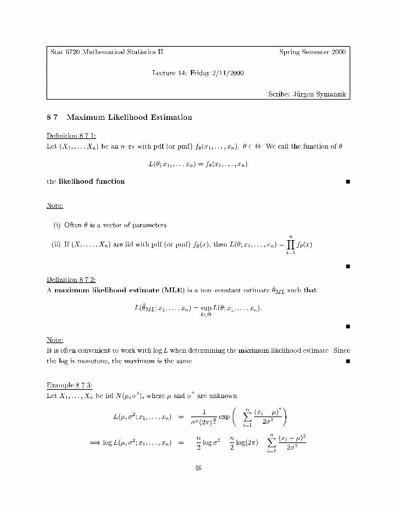
8.7 Maximum Likelihood Estimation
De�nition 8.7.1:
Let (X1; : : : ;Xn) be an n{rv with pdf (or pmf) f�(x1; : : : ; xn); � 2 �. We call the function of �
L(�;x1; : : : ; xn) = f�(x1; : : : ; xn)
the likelihood function.
Note:
(i) Often � is a vector of parameters.
(ii) If (X1; : : : ;Xn) are iid with pdf (or pmf) f�(x), then L(�;x1; : : : ; xn) =nYi=1
f�(x).
De�nition 8.7.2:
A maximum likelihood estimate (MLE) is a non{constant estimate �̂ML such that
L(�̂ML;x1; : : : ; xn) = sup�2�
L(�;x1; : : : ; xn):
Note:
It is often convenient to work with logL when determining the maximum likelihood estimate. Since
the log is monotone, the maximum is the same.
Example 8.7.3:
Let X1; : : : ; Xn be iid N(�; �2), where � and �2 are unknown.
L(�; �2;x1; : : : ; xn) =1
�n(2�)n2
exp
�
nXi=1
(xi � �)2
2�2
!
=) logL(�; �2;x1; : : : ; xn) = �n2log �2 � n
2log(2�) �
nXi=1
(xi � �)2
2�2
46
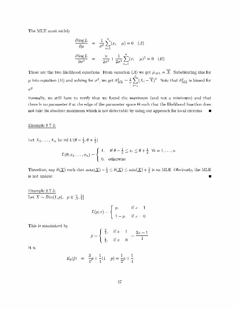
The MLE must satisfy
@ logL
@�=
1
�2
nXi=1
(xi � �) = 0 (A)
@ logL
@�2= � n
2�2+
1
2�4
nXi=1
(xi � �)2 = 0 (B)
These are the two likelihood equations. From equation (A) we get �̂ML = X . Substituting this for
� into equation (B) and solving for �2, we get �̂2ML
= 1n
nXi=1
(Xi�X)2. Note that �̂2ML
is biased for
�2.
Formally, we still have to verify that we found the maximum (and not a minimum) and that
there is no parameter � at the edge of the parameter space � such that the likelihood function does
not take its absolute maximum which is not detectable by using our approach for local extrema.
Example 8.7.4:
Let X1; : : : ; Xn be iid U(� � 12 ; � +
12).
L(�;x1; : : : ; xn) =
8<: 1; if � � 12 � xi � � + 1
2 8i = 1; : : : ; n
0; otherwise
Therefore, any �̂(X) such that max(X)� 12 � �̂(X) � min(X)+ 1
2 is an MLE. Obviously, the MLE
is not unique.
Example 8.7.5:
Let X � Bin(1; p); p 2 [14 ;34 ].
L(p;x) =
8<: p; if x = 1
1� p; if x = 0
This is maximized by
p̂ =
8<:34 ; if x = 1
14 ; if x = 0
=2x+ 1
4
It is
Ep(p̂) =3
4p+
1
4(1� p) =
1
2p+
1
4
47
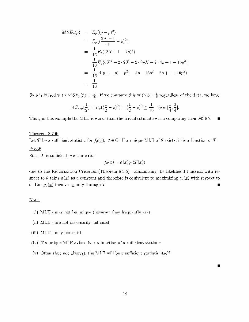
MSEp(p̂) = Ep((p̂� p)2)
= Ep((2X + 1
4� p)2)
=1
16Ep((2X + 1� 4p)2)
=1
16Ep(4X
2 + 2 � 2X � 2 � 8pX � 2 � 4p+ 1 + 16p2)
=1
16(4(p(1 � p) + p2) + 4p� 16p2 � 8p+ 1 + 16p2)
=1
16
So p̂ is biased with MSEp(p̂) =116 . If we compare this with ~p = 1
2 regardless of the data, we have
MSEp(1
2) = Ep((
1
2� p)2) = (
1
2� p)2 � 1
168p 2 [
1
4;3
4]:
Thus, in this example the MLE is worse than the trivial estimate when comparing their MSE's.
Theorem 8.7.6:
Let T be a su�cient statistic for f�(x); � 2 �. If a unique MLE of � exists, it is a function of T .
Proof:
Since T is su�cient, we can write
f�(x) = h(x)g�(T (x))
due to the Factorization Criterion (Theorem 8.3.5). Maximizing the likelihood function with re-
spect to � takes h(x) as a constant and therefore is equivalent to maximizing g�(x) with respect to
�. But g�(x) involves x only through T .
Note:
(i) MLE's may not be unique (however they frequently are).
(ii) MLE's are not necessarily unbiased.
(iii) MLE's may not exist.
(iv) If a unique MLE exists, it is a function of a su�cient statistic.
(v) Often (but not always), the MLE will be a su�cient statistic itself.
48
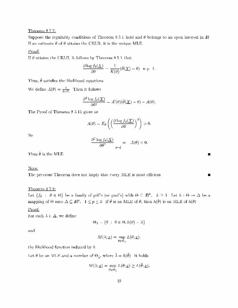
Theorem 8.7.7:
Suppose the regularity conditions of Theorem 8.5.1 hold and � belongs to an open interval in IR.
If an estimate �̂ of � attains the CRLB, it is the unique MLE.
Proof:
If �̂ attains the CRLB, it follows by Theorem 8.5.1 that
@ log f�(X)
@�=
1
K(�)(�̂(X)� �) w.p. 1:
Thus, �̂ satis�es the likelihood equations.
We de�ne A(�) = 1K(�) . Then it follows
@2 log f�(X)
@�2= A0(�)(�̂(X)� �)�A(�):
The Proof of Theorem 8.5.11 gives us
A(�) = E�
�@ log f�(X)
@�
�2!> 0:
So@2 log f�(X)
@�2
������=�̂
= �A(�) < 0:
Thus �̂ is the MLE.
Note:
The previous Theorem does not imply that every MLE is most e�cient.
Theorem 8.7.8:
Let ff� : � 2 �g be a family of pdf's (or pmf's) with � � IRk; k � 1. Let h : � ! � be a
mapping of � onto � � IRp; 1 � p � k. If �̂ is an MLE of �, then h(�̂) is an MLE of h(�).
Proof:
For each � 2 �, we de�ne
�� = f� : � 2 �; h(�) = �g
and
M(�;x) = sup�2��
L(�;x);
the likelihood function induced by h.
Let �̂ be an MLE and a member of ��̂, where �̂ = h(�̂). It holds
M(�̂;x) = sup�2�
�̂
L(�;x) � L(�̂;x);
49
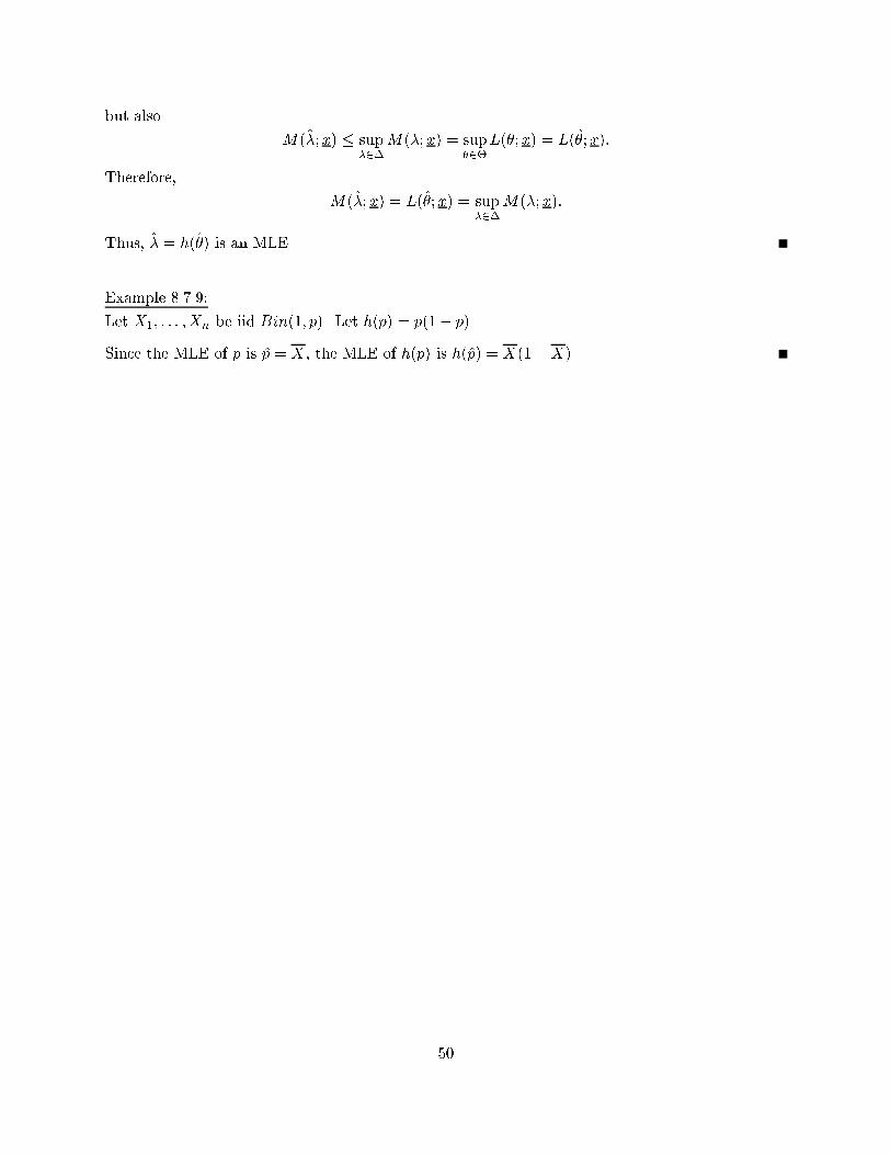
but also
M(�̂;x) � sup�2�
M(�;x) = sup�2�
L(�;x) = L(�̂;x):
Therefore,
M(�̂;x) = L(�̂;x) = sup�2�
M(�;x):
Thus, �̂ = h(�̂) is an MLE.
Example 8.7.9:
Let X1; : : : ; Xn be iid Bin(1; p). Let h(p) = p(1� p).
Since the MLE of p is p̂ = X , the MLE of h(p) is h(p̂) = X(1�X).
50
Stat 6720 Mathematical Statistics II Spring Semester 2000
Lecture 15: Monday 2/14/2000
Scribe: J�urgen Symanzik
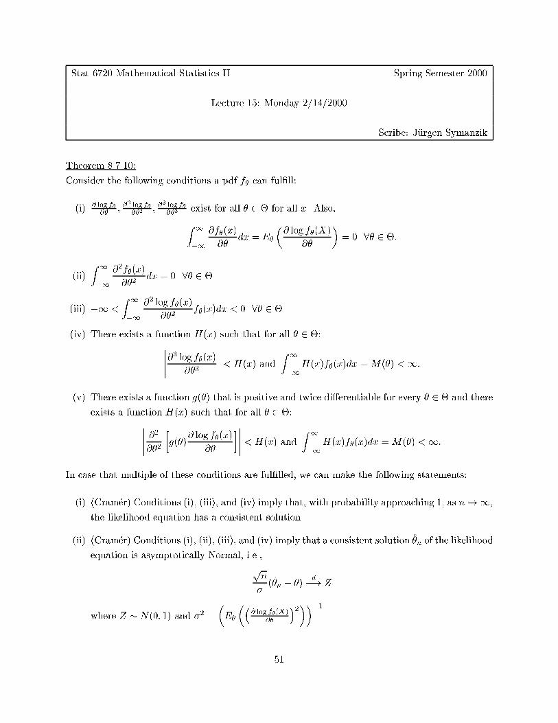
Theorem 8.7.10:
Consider the following conditions a pdf f� can ful�ll:
(i) @ log f�@�
;@2 log f�@�2
;@3 log f�@�3
exist for all � 2 � for all x. Also,Z 1
�1
@f�(x)
@�dx = E�
�@ log f�(X)
@�
�= 0 8� 2 �:
(ii)
Z 1
�1
@2f�(x)
@�2dx = 0 8� 2 �.
(iii) �1 <
Z 1
�1
@2 log f�(x)
@�2f�(x)dx < 0 8� 2 �.
(iv) There exists a function H(x) such that for all � 2 �:�����@3 log f�(x)@�3
����� < H(x) and
Z 1
�1H(x)f�(x)dx =M(�) <1:
(v) There exists a function g(�) that is positive and twice di�erentiable for every � 2 � and there
exists a function H(x) such that for all � 2 �:����� @2@�2�g(�)
@ log f�(x)
@�
������ < H(x) and
Z 1
�1H(x)f�(x)dx =M(�) <1:
In case that multiple of these conditions are ful�lled, we can make the following statements:
(i) (Cram�er) Conditions (i), (iii), and (iv) imply that, with probability approaching 1, as n!1,
the likelihood equation has a consistent solution.
(ii) (Cram�er) Conditions (i), (ii), (iii), and (iv) imply that a consistent solution �̂n of the likelihood
equation is asymptotically Normal, i.e.,
pn
�(�̂n � �)
d�! Z
where Z � N(0; 1) and �2 =
�E�
��@ log f�(X)
@�
�2���1.
51

(iii) (Kulldorf) Conditions (i), (iii), and (v) imply that, with probability approaching 1, as n!1,
the likelihood equation has a consistent solution.
(iv) (Kulldorf) Conditions (i), (ii), (iii), and (v) imply that a consistent solution �̂n of the likelihood
equation is asymptotically Normal.
Note:
In case of a pmf f�, we can de�ne similar conditions as in Theorem 8.7.10.
52
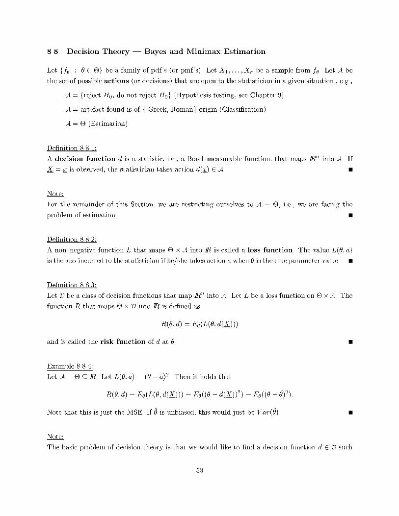
8.8 Decision Theory | Bayes and Minimax Estimation
Let ff� : � 2 �g be a family of pdf's (or pmf's). Let X1; : : : ;Xn be a sample from f�. Let A be
the set of possible actions (or decisions) that are open to the statistician in a given situation , e.g.,
A = freject H0, do not reject H0g (Hypothesis testing, see Chapter 9)
A = artefact found is of f Greek, Romang origin (Classi�cation)
A = � (Estimation)
De�nition 8.8.1:
A decision function d is a statistic, i.e., a Borel{measurable function, that maps IRn into A. If
X = x is observed, the statistician takes action d(x) 2 A.
Note:
For the remainder of this Section, we are restricting ourselves to A = �, i.e., we are facing the
problem of estimation.
De�nition 8.8.2:
A non{negative function L that maps � � A into IR is called a loss function. The value L(�; a)
is the loss incurred to the statistician if he/she takes action a when � is the true parameter value.
De�nition 8.8.3:
Let D be a class of decision functions that map IRn into A. Let L be a loss function on ��A. Thefunction R that maps �� D into IR is de�ned as
R(�; d) = E�(L(�; d(X)))
and is called the risk function of d at �.
Example 8.8.4:
Let A = � � IR. Let L(�; a) = (� � a)2. Then it holds that
R(�; d) = E�(L(�; d(X))) = E�((� � d(X))2) = E�((� � �̂)2):
Note that this is just the MSE. If �̂ is unbiased, this would just be V ar(�̂).
Note:
The basic problem of decision theory is that we would like to �nd a decision function d 2 D such
53
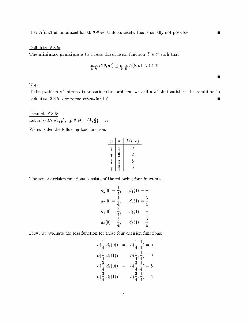
that R(�; d) is minimized for all � 2 �. Unfortunately, this is usually not possible.
De�nition 8.8.5:
The minimax principle is to choose the decision function d� 2 D such that
max�2�
R(�; d�) � max�2�
R(�; d) 8d 2 D:
Note:
If the problem of interest is an estimation problem, we call a d� that satisi�es the condition in
De�nition 8.8.5 a minimax estimate of �.
Example 8.8.6:
Let X � Bin(1; p); p 2 � = f14 ;34g = A.
We consider the following loss function:
p a L(p; a)14
14 0
14
34 2
34
14 5
34
34 0
The set of decision functions consists of the following four functions:
d1(0) =1
4; d1(1) =
1
4
d2(0) =1
4; d2(1) =
3
4
d3(0) =3
4; d3(1) =
1
4
d4(0) =3
4; d4(1) =
3
4
First, we evaluate the loss function for these four decision functions:
L(1
4; d1(0)) = L(
1
4;1
4) = 0
L(1
4; d1(1)) = L(
1
4;1
4) = 0
L(3
4; d1(0)) = L(
3
4;1
4) = 5
L(3
4; d1(1)) = L(
3
4;1
4) = 5
54
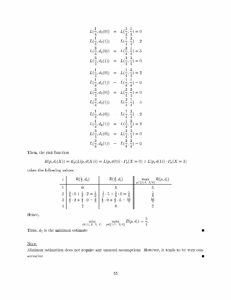
L(1
4; d2(0)) = L(
1
4;1
4) = 0
L(1
4; d2(1)) = L(
1
4;3
4) = 2
L(3
4; d2(0)) = L(
3
4;1
4) = 5
L(3
4; d2(1)) = L(
3
4;3
4) = 0
L(1
4; d3(0)) = L(
1
4;3
4) = 2
L(1
4; d3(1)) = L(
1
4;1
4) = 0
L(3
4; d3(0)) = L(
3
4;3
4) = 0
L(3
4; d3(1)) = L(
3
4;1
4) = 5
L(1
4; d4(0)) = L(
1
4;3
4) = 2
L(1
4; d4(1)) = L(
1
4;3
4) = 2
L(3
4; d4(0)) = L(
3
4;3
4) = 0
L(3
4; d4(1)) = L(
3
4;3
4) = 0
Then, the risk function
R(p; di(X)) = Ep(L(p; d(X))) = L(p; d(0)) � Pp(X = 0) + L(p; d(1)) � Pp(X = 1)
takes the following values:
i R(14 ; di) R(34 ; di) maxp2f1=4; 3=4g
R(p; di)
1 0 5 5
2 34 � 0 +
14 � 2 =
12
14 � 5 +
34 � 0 =
54
54
3 34 � 2 +
14 � 0 =
32
14 � 0 +
34 � 5 =
154
154
4 2 0 2
Hence,
mini2f1; 2; 3; 4g
maxp2f1=4; 3=4g
R(p; di) =5
4:
Thus, d2 is the minimax estimate.
Note:
Minimax estimation does not require any unusual assumptions. However, it tends to be very con-
servative.
55
Stat 6720 Mathematical Statistics II Spring Semester 2000
Lecture 16: Wednesday 2/16/2000
Scribe: J�urgen Symanzik
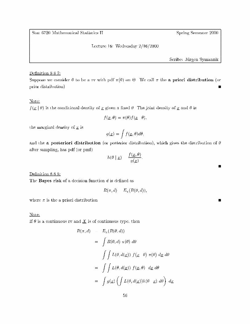
De�nition 8.8.7:
Suppose we consider � to be a rv with pdf �(�) on �. We call � the a priori distribution (or
prior distribution).
Note:
f(x j �) is the conditional density of x given a �xed �. The joint density of x and � is
f(x; �) = �(�)f(x j �);
the marginal density of x is
g(x) =
Zf(x; �)d�;
and the a posteriori distribution (or posterior distribution), which gives the distribution of �
after sampling, has pdf (or pmf)
h(� j x) = f(x; �)
g(x):
De�nition 8.8.8:
The Bayes risk of a decision function d is de�ned as
R(�; d) = E�(R(�; d));
where � is the a priori distribution.
Note:
If � is a continuous rv and X is of continuous type, then
R(�; d) = E�(R(�; d))
=
ZR(�; d) �(�) d�
=
Z ZL(�; d(x)) f(x j �) �(�) dx d�
=
Z ZL(�; d(x)) f(x; �) dx d�
=
Zg(x)
�ZL(�; d(x))h(� j x) d�
�dx
56
Similar expressions can be written if � and/or X are discrete.
De�nition 8.8.9:
A decision function d� is called a Bayes rule if d� minimizes the Bayes risk, i.e., if
R(�; d�) = infd2D
R(�; d):
Theorem 8.8.10:
Let A = � � IR. Let L(�; d(x)) = (� � d(x))2. In this case, a Bayes rule is
d(x) = E(� j X = x):
Proof:
Minimizing
R(�; d) =
Zg(x)
�Z(� � d(x))2h(� j x) d�
�dx;
where g is the marginal pdf of X and h is the conditional pdf of � given x, is the same as minimizingZ(� � d(x))2h(� j x) d�:
However, this is minimized when d(x) = E(� j X = x).
Note:
Under the conditions of Theorem 8.8.10, d(x) = E(� j X = x) is called the Bayes estimate.
Example 8.8.11:
Let X � Bin(n; p). Let L(p; d(x)) = (p� d(x))2.
Let �(p) = 1 8p 2 (0; 1), i.e., � � U(0; 1), be the a priori distribution of p.
Then it holds:
f(x; �) =
n
x
!px(1� p)n�x
g(x) =
Z 1
0
n
x
!px(1� p)n�xdp
h(p j x) =
�n
x
�px(1� p)n�xZ 1
0
n
x
!px(1� p)n�xdp
57
=px(1� p)n�xZ 1
0px(1� p)n�xdp
E(p j x) =
Z 1
0ph(p j x)dp
=
Z 1
0p
n
x
!px(1� p)n�xdp
Z 1
0
n
x
!px(1� p)n�xdp
=
Z 1
0px+1(1� p)n�xdpZ 1
0px(1� p)n�xdp
=x+ 1
n+ 2
Thus, the Bayes rule is
p̂Bayes = d�(X) =X + 1
n+ 2:
The Bayes risk of d�(X) is
R(�; d�(X)) = E�(R(p; d�(X)))
=
Z 1
0�(p)R(p; d�(x))dp
=
Z 1
0�(p)
nXx=0
L(p; d�(x))f(x j p)dp
=
Z 1
0�(p)
nXx=0
(x+ 1
n+ 2� p)2f(x j p)dp
=
Z 1
0Ep
�(X + 1
n+ 2� p)2
�dp
=
Z 1
0Ep
�(X + 1
n+ 2)2 � 2p
X + 1
n+ 2+ p2
�dp
=1
(n+ 2)2
Z 1
0Ep
�(X + 1)2 � 2p(n+ 2)(X + 1) + p2(n+ 2)2
�dp
...
=1
(n+ 2)2
Z 1
0(np(1� p) + (1� 2p)2)dp
...
58
=1
6(n+ 2)
Now we compare the Bayes rule d�(X) with the MLE p̂ML = X
n. This estimate has Bayes risk
R(�;X
n) =
Z 1
0Ep((
X
n� p)2)dp
=
Z 1
0
1
n2Ep((X � np)2)dp
=
Z 1
0
p(1� p)
ndp
=1
6n
which is, as expected, larger than the Bayes risk of d�(X).
Theorem 8.8.12:
Let ff� : � 2 �g be a family of pdf's (or pmf's). Suppose that an estimate d� of � is a Bayes
estimate corresponding to some prior distribution � on �. If the risk function R(�; d�) is constant
on �, then d� is a minimax estimate of �.
59
Stat 6720 Mathematical Statistics II Spring Semester 2000
Lecture 17: Friday 2/18/2000
Scribe: J�urgen Symanzik
9 Hypothesis Testing
9.1 Fundamental Notions
We assume that X = (X1; : : : ; Xn) is a random sample from a population distribution F�; � 2 � �IRk, where the functional form of F� is known, except for the parameter �. We also assume that �
contains at least two points.
De�nition 9.1.1:
A parametric hypothesis is an assumption about the unknown parameter �.
The null hypothesis is of the form
H0 : � 2 �0 � �:
The alternative hypothesis is of the form
H1 : � 2 �1 = ���0:
De�nition 9.1.2:
If �0 (or �1) contains only one point, we say that H0 and �0 (or H1 and �1) are simple. In this
case, the distribution of X is completely speci�ed under the null (or alternative) hypothesis.
If �0 (or �1) contains more than one point, we say that H0 and �0 (or H1 and �1) are composite.
Example 9.1.3:
Let X1; : : : ;Xn be iid Bin(1; p). Examples for hypotheses are p = 12 (simple), p � 1
2 (composite),
p 6= 14 (composite), etc.
60
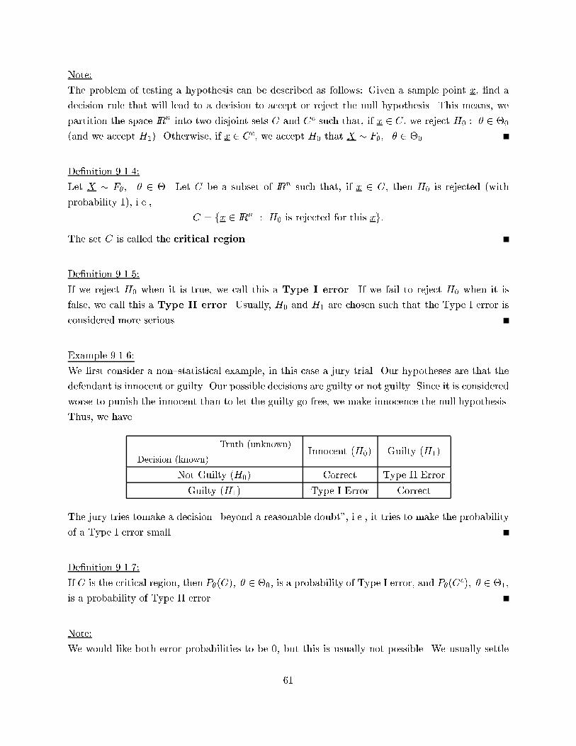
Note:
The problem of testing a hypothesis can be described as follows: Given a sample point x, �nd a
decision rule that will lead to a decision to accept or reject the null hypothesis. This means, we
partition the space IRn into two disjoint sets C and Cc such that, if x 2 C, we reject H0 : � 2 �0
(and we accept H1). Otherwise, if x 2 Cc, we accept H0 that X � F�; � 2 �0.
De�nition 9.1.4:
Let X � F�; � 2 �. Let C be a subset of IRn such that, if x 2 C, then H0 is rejected (with
probability 1), i.e.,
C = fx 2 IRn : H0 is rejected for this xg:
The set C is called the critical region.
De�nition 9.1.5:
If we reject H0 when it is true, we call this a Type I error. If we fail to reject H0 when it is
false, we call this a Type II error. Usually, H0 and H1 are chosen such that the Type I error is
considered more serious.
Example 9.1.6:
We �rst consider a non{statistical example, in this case a jury trial. Our hypotheses are that the
defendant is innocent or guilty. Our possible decisions are guilty or not guilty. Since it is considered
worse to punish the innocent than to let the guilty go free, we make innocence the null hypothesis.
Thus, we have
Truth (unknown)
Decision (known)Innocent (H0) Guilty (H1)
Not Guilty (H0) Correct Type II Error
Guilty (H1) Type I Error Correct
The jury tries tomake a decision \beyond a reasonable doubt", i.e., it tries to make the probability
of a Type I error small.
De�nition 9.1.7:
If C is the critical region, then P�(C); � 2 �0, is a probability of Type I error, and P�(Cc); � 2 �1,
is a probability of Type II error.
Note:
We would like both error probabilities to be 0, but this is usually not possible. We usually settle
61
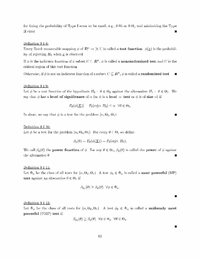
for �xing the probability of Type I error to be small, e.g., 0.05 or 0.01, and minimizing the Type
II error.
De�nition 9.1.8:
Every Borel{measurable mapping � of IRn ! [0; 1] is called a test function. �(x) is the probabil-
ity of rejecting H0 when x is observed.
If � is the indicator function of a subset C � IRn, � is called a nonrandomized test and C is the
critical region of this test function.
Otherwise, if � is not an indicator function of a subset C � IRn, � is called a randomized test.
De�nition 9.1.9:
Let � be a test function of the hypothesis H0 : � 2 �0 against the alternative H1 : � 2 �1. We
say that � has a level of signi�cance of � (or � is a level{�{test or � is of size �) if
E�(�(X)) = P�(rejct H0) � � 8� 2 �0:
In short, we say that � is a test for the problem (�;�0;�1).
De�nition 9.1.10:
Let � be a test for the problem (�;�0;�1). For every � 2 �, we de�ne
��(�) = E�(�(X)) = P�(rejct H0):
We call ��(�) the power function of �. For any � 2 �1, ��(�) is called the power of � against
the alternative �.
De�nition 9.1.11:
Let �� be the class of all tests for (�;�0;�1). A test �0 2 �� is called a most powerful (MP)
test against an alternative � 2 �1 if
��0(�) � ��(�) 8� 2 ��:
De�nition 9.1.12:
Let �� be the class of all tests for (�;�0;�1). A test �0 2 �� is called a uniformly most
powerful (UMP) test if
��0(�) � ��(�) 8� 2 �� 8� 2 �1:
62
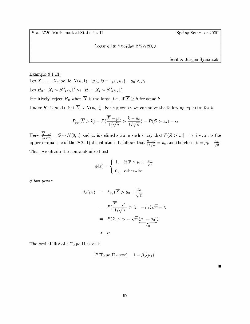
Stat 6720 Mathematical Statistics II Spring Semester 2000
Lecture 18: Tuesday 2/22/2000
Scribe: J�urgen Symanzik
Example 9.1.13:
Let X1; : : : ; Xn be iid N(�; 1); � 2 � = f�0; �1g; �0 < �1.
Let H0 : Xi � N(�0; 1) vs. H1 : Xi � N(�1; 1).
Intuitively, reject H0 when X is too large, i.e., if X � k for some k.
Under H0 it holds that X � N(�0;1n. For a given �, we can solve the following equation for k:
P�0(X > k) = P (X � �0
1=pn
>k � �0
1=pn) = P (Z > z�) = �
Here, X��01=pn= Z � N(0; 1) and z� is de�ned such in such a way that P (Z > z�) = �, i.e., z� is the
upper �{quantile of the N(0; 1) distribution. It follows that k��01=pn= z� and therefore, k = �0+
z�pn.
Thus, we obtain the nonrandomized test
�(x) =
8<: 1; if x > �0 +z�pn
0; otherwise
� has power
��(�1) = P�1(X > �0 +z�pn
= P (X � �1
1=pn
> (�0 � �1)pn+ z�
= P (Z > z� �pn (�1 � �0)| {z }
>0
)
> �
The probability of a Type II error is
P (Type II error) = 1� ��(�1):
63
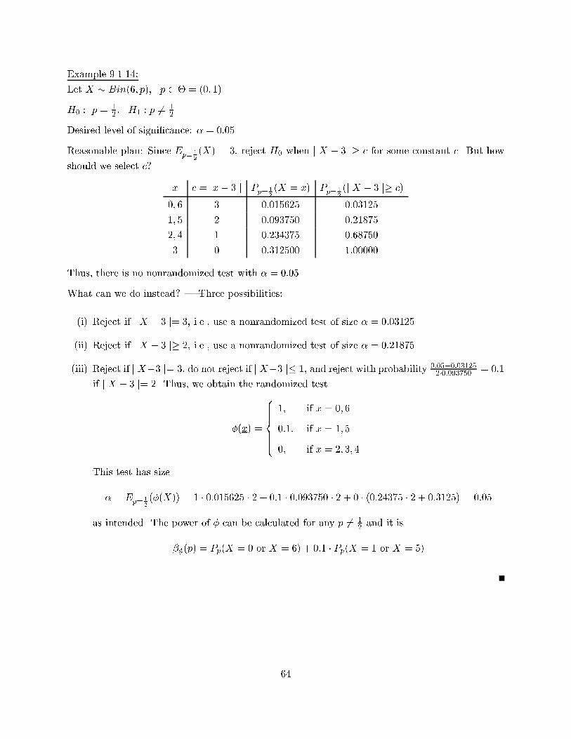
Example 9.1.14:
Let X � Bin(6; p); p 2 � = (0; 1).
H0 : p =12 ; H1 : p 6= 1
2 .
Desired level of signi�cance: � = 0:05.
Reasonable plan: Since Ep= 1
2(X) = 3, reject H0 when j X � 3 j� c for some constant c. But how
should we select c?
x c =j x� 3 j Pp= 1
2(X = x) P
p= 12(j X � 3 j� c)
0; 6 3 0:015625 0:03125
1; 5 2 0:093750 0:21875
2; 4 1 0:234375 0:68750
3 0 0:312500 1:00000
Thus, there is no nonrandomized test with � = 0:05.
What can we do instead? | Three possibilities:
(i) Reject if j X � 3 j= 3, i.e., use a nonrandomized test of size � = 0:03125.
(ii) Reject if j X � 3 j� 2, i.e., use a nonrandomized test of size � = 0:21875.
(iii) Reject if j X�3 j= 3, do not reject if j X�3 j� 1, and reject with probability 0:05�0:031252�0:093750 = 0:1
if j X � 3 j= 2. Thus, we obtain the randomized test
�(x) =
8>>>><>>>>:1; if x = 0; 6
0:1; if x = 1; 5
0; if x = 2; 3; 4
This test has size
� = Ep= 1
2(�(X)) = 1 � 0:015625 � 2 + 0:1 � 0:093750 � 2 + 0 � (0:24375 � 2 + 0:3125) = 0:05
as intended. The power of � can be calculated for any p 6= 12 and it is
��(p) = Pp(X = 0 or X = 6) + 0:1 � Pp(X = 1 or X = 5)
64
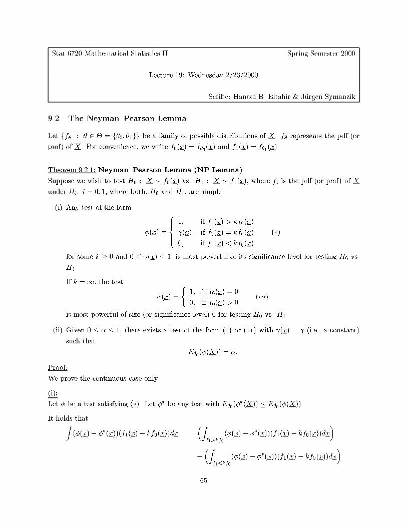
Stat 6720 Mathematical Statistics II Spring Semester 2000
Lecture 19: Wednesday 2/23/2000
Scribe: Hanadi B. Eltahir & J�urgen Symanzik
9.2 The Neyman{Pearson Lemma
Let ff� : � 2 � = f�0; �1gg be a family of possible distributions of X. f� represents the pdf (or
pmf) of X . For convenience, we write f0(x) = f�0(x) and f1(x) = f�1(x).
Theorem 9.2.1: Neyman{Pearson Lemma (NP Lemma)
Suppose we wish to test H0 : X � f0(x) vs. H1 : X � f1(x), where fi is the pdf (or pmf) of X
under Hi; i = 0; 1, where both, H0 and H1, are simple.
(i) Any test of the form
�(x) =
8>><>>:1; if f1(x) > kf0(x)
(x); if f1(x) = kf0(x)
0; if f1(x) < kf0(x)
(�)
for some k � 0 and 0 � (x) � 1, is most powerful of its signi�cance level for testing H0 vs.
H1.
If k =1, the test
�(x) =
(1; if f0(x) = 0
0; if f0(x) > 0(��)
is most powerful of size (or signi�cance level) 0 for testing H0 vs. H1.
(ii) Given 0 � � � 1, there exists a test of the form (�) or (��) with (x) = (i.e., a constant)
such that
E�0(�(X)) = �:
Proof:
We prove the continuous case only.
(i):
Let � be a test satisfying (�). Let �� be any test with E�0(��(X)) � E�0
(�(X)).
It holds thatZ(�(x)� ��(x))(f1(x)� kf0(x))dx =
�Zf1>kf0
(�(x)� ��(x))(f1(x)� kf0(x))dx
�
+
�Zf1<kf0
(�(x)� ��(x))(f1(x)� kf0(x))dx
�
65
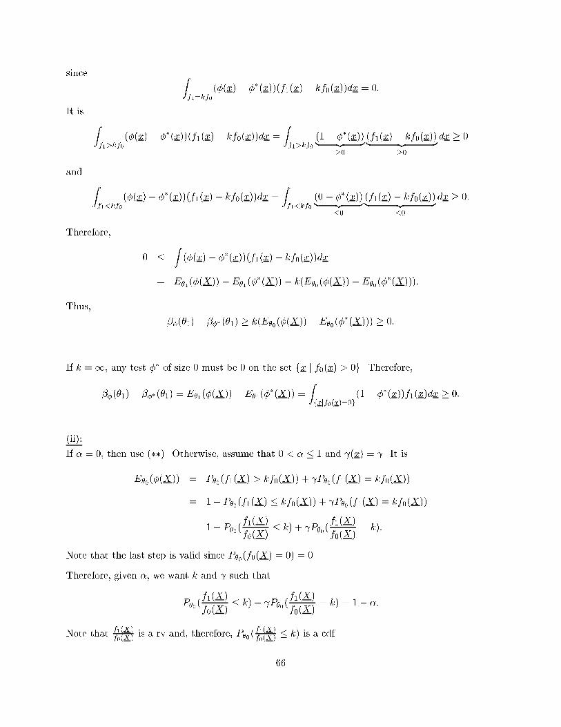
since Zf1=kf0
(�(x)� ��(x))(f1(x)� kf0(x))dx = 0:
It is Zf1>kf0
(�(x)� ��(x))(f1(x)� kf0(x))dx =
Zf1>kf0
(1� ��(x))| {z }�0
(f1(x)� kf0(x))| {z }�0
dx � 0
and Zf1<kf0
(�(x)� ��(x))(f1(x)� kf0(x))dx =
Zf1<kf0
(0� ��(x))| {z }�0
(f1(x)� kf0(x))| {z }�0
dx � 0:
Therefore,
0 �Z(�(x)� ��(x))(f1(x)� kf0(x))dx
= E�1(�(X))�E�1
(��(X))� k(E�0(�(X))�E�0
(��(X))):
Thus,
��(�1)� ���(�1) � k(E�0(�(X))�E�0
(��(X))) � 0:
If k =1, any test �� of size 0 must be 0 on the set fx j f0(x) > 0g. Therefore,
��(�1)� ���(�1) = E�1(�(X))�E�1
(��(X)) =
Zfxjf0(x)=0g
(1� ��(x))f1(x)dx � 0:
(ii):
If � = 0, then use (��). Otherwise, assume that 0 < � � 1 and (x) = . It is
E�0(�(X)) = P�0(f1(X) > kf0(X)) + P�0(f1(X) = kf0(X))
= 1� P�0(f1(X) � kf0(X)) + P�0(f1(X) = kf0(X))
= 1� P�0(f1(X)
f0(X)� k) + P�0(
f1(X)
f0(X)= k):
Note that the last step is valid since P�0(f0(X) = 0) = 0.
Therefore, given �, we want k and such that
P�0(f1(X)
f0(X)� k)� P�0(
f1(X)
f0(X)= k) = 1� �:
Note thatf1(X)f0(X) is a rv and, therefore, P�0(
f1(X)f0(X) � k) is a cdf.
66
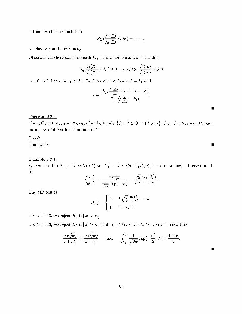
If there exists a k0 such that
P�0(f1(X)
f0(X)� k0) = 1� �;
we choose = 0 and k = k0.
Otherwise, if there exists no such k0, then there exists a k1 such that
P�0(f1(X)
f0(X)< k1) � 1� � < P�0(
f1(X)
f0(X)� k1);
i.e., the cdf has a jump at k1. In this case, we choose k = k1 and
=P�0(
f1(X)f0(X) � k1)� (1� �)
P�0(f1(X)f0(X)
= k1):
Theorem 9.2.2:
If a su�cient statistic T exists for the family ff� : � 2 � = f�0; �1gg, then the Neyman{Pearson
most powerful test is a function of T .
Proof:
Homework
Example 9.2.3:
We want to test H0 : X � N(0; 1) vs. H1 : X � Cauchy(1; 0), based on a single observation. It
isf1(x)
f0(x)=
1�
11+x2
1p2�
exp(�x2
2 )=
r2
�
exp(x2
2 )
1 + x2:
The MP test is
�(x) =
8><>: 1; ifq
2�
exp(x2
2)
1+x2> k
0; otherwise
If � < 0:113, we reject H0 if j x j> z�2.
If � > 0:113, we reject H0 if j x j> k1 or if j x j< k2, where k1 > 0, k2 > 0, such that
exp(k21
2 )
1 + k21=
exp(k22
2 )
1 + k22and
Zk1
k2
1p2�
exp(�x2
2)dx =
1� �
2:
67
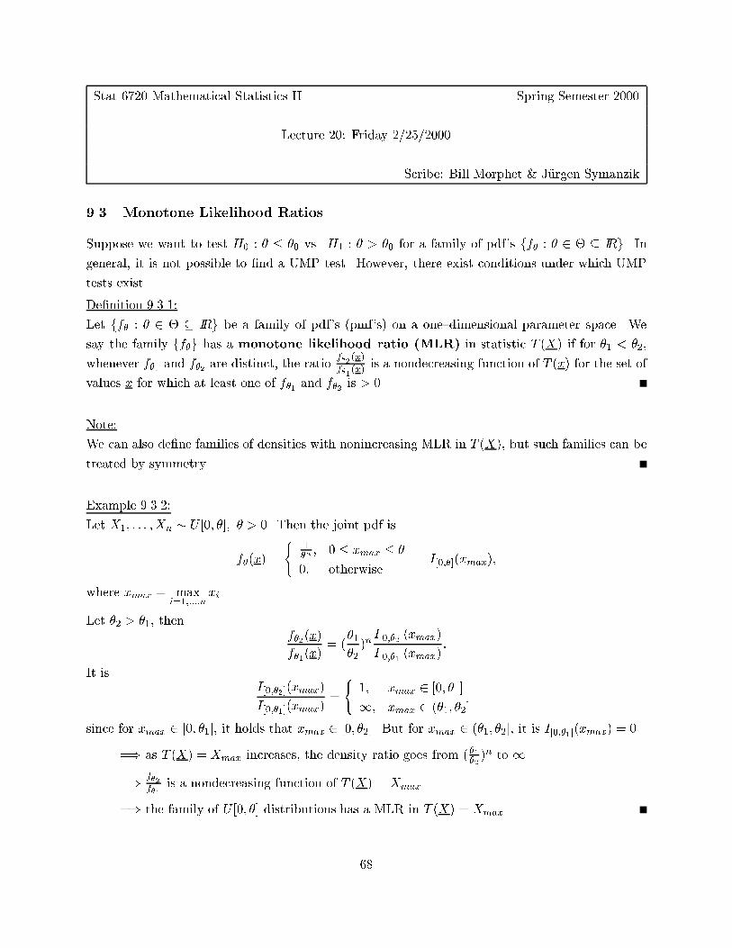
Stat 6720 Mathematical Statistics II Spring Semester 2000
Lecture 20: Friday 2/25/2000
Scribe: Bill Morphet & J�urgen Symanzik
9.3 Monotone Likelihood Ratios
Suppose we want to test H0 : � � �0 vs. H1 : � > �0 for a family of pdf's ff� : � 2 � � IRg. Ingeneral, it is not possible to �nd a UMP test. However, there exist conditions under which UMP
tests exist.
De�nition 9.3.1:
Let ff� : � 2 � � IRg be a family of pdf's (pmf's) on a one{dimensional parameter space. We
say the family ff�g has a monotone likelihood ratio (MLR) in statistic T (X) if for �1 < �2,
whenever f�1 and f�2 are distinct, the ratiof�2
(x)
f�1(x)
is a nondecreasing function of T (x) for the set of
values x for which at least one of f�1 and f�2 is > 0.
Note:
We can also de�ne families of densities with nonincreasing MLR in T (X), but such families can be
treated by symmetry.
Example 9.3.2:
Let X1; : : : ; Xn � U [0; �]; � > 0. Then the joint pdf is
f�(x) =
(1�n; 0 � xmax � �
0; otherwise= I[0;�](xmax);
where xmax = maxi=1;:::;n
xi.
Let �2 > �1, thenf�2(x)
f�1(x)= (
�1
�2)nI[0;�2](xmax)
I[0;�1](xmax):
It isI[0;�2](xmax)
I[0;�1](xmax)=
(1; xmax 2 [0; �1]
1; xmax 2 (�1; �2]
since for xmax 2 [0; �1], it holds that xmax 2 [0; �2]. But for xmax 2 (�1; �2], it is I[0;�1](xmax) = 0.
=) as T (X) = Xmax increases, the density ratio goes from ( �1�2)n to 1.
=) f�2
f�1is a nondecreasing function of T (X) = Xmax
=) the family of U [0; �] distributions has a MLR in T (X) = Xmax
68
Theorem 9.3.3:
The one{parameter exponential family f�(x) = exp(Q(�)T (x) +D(�) + S(x)), where Q(�) is non-
decreasing, has a MLR in T (X).
Proof:
Homework.
Example 9.3.4:
Let X = (X1; � � � ;Xn) be a random sample from the Poisson family with parameter � > 0. Then
the joint pdf is
f�(x) =nYi=1
�e���xi
1
xi!
�= e�n��
Pn
i=1xi
nYi=1
1
xi!= exp
�n�+
nXi=1
xi � log(�) �nXi=1
log(xi!)
!;
which belongs to the one{parameter exponential family.
Since Q(�) = log(�) is a nondecreasing function of �, it follows by Theorem 9.3.3 that the Poisson
family with parameter � > 0 has a MLR in T (X) =nXi=1
Xi.
We can verify this result by De�nition 9.3.1:
f�2(x)
f�1(x)=�
Pxi
2
�
Pxi
1
e�n�2
e�n�1=
��2
�1
�Pxi
e�n(�2��1):
If �2 > �1, then�2
�1> 1 and
��2
�1
�Pxi
is a nondecreasing function ofPxi.
Therefore, f� has a MLR in T (X) =nXi=1
Xi.
Theorem 9.3.5:
Let X � f�; � 2 � � IR, where the family ff�g has a MLR in T (X).
For testing H0 : � � �0 vs. H1 : � > �0; �0 2 �; any test of the form
�(x) =
8>><>>:1; if T (x) > t0
; if T (x) = t0
0; if T (x) < t0
(�)
has a nondecreasing power function and is UMP of its size E�0(�(X)) = �, if the size is not 0.
Also, for every 0 � � � 1 and every �0 2 �, there exists a t0 and a (�1 � t0 � 1; 0 � � 1),
such that the test of form (�) is the UMP size � test of H0 vs. H1:
69
Proof:
\=)":
Let �1 < �2; �1; �2 2 � and suppose E�1(�(X)) > 0. Since f� has a MLR in T ,
f�2(x)
f�1(x)
is a
nondecreasing function of T . Therefore, any test of form (�) is equivalent to a test
�(x) =
8>>>>><>>>>>:1; if
f�2(x)
f�1(x)
> k
; iff�2
(x)
f�1(x) = k
0; iff�2
(x)
f�1(x)
< k
(��)
which by the Neyman{Pearson Lemma (Theorem 9.2.1) is MP of size � for testing H0 : � = �1 vs.
H1 : � = �2.
Let �� be the class of tests of size �, and let �t 2 �� be the trivial test �t(x) = � 8x. Then �thas size and power �. The power of the MP test � of form (�) must be at least � as the MP test
� cannot have power less than the trivial test �t, i.e,
E�2(�(X)) � E�2
(�t(X)) = � = E�1(�(X)):
Thus, for �2 > �1,
E�2(�(X)) � E�1
(�(X));
i.e., the power function of the test � of form (�) is a nondecreasing function of �.
Now let �1 = �0 and �2 > �0. We know that a test � of form (�) is MP for H0 : � = �0 vs.
H1 : � = �2 > �0, provided that its size � = E�0(�(X)) is > 0.
Notice that the test � of form (�) does not depend on �2. It only depends on t0 and . Therefore,
the test � of form (�) is MP for all �2 2 �1. Thus, this test is UMP for simple H0 : � = �0 vs.
composite H1 : � > �0 with size E�0(�(X)) = �0.
Since � is UMP for a class �00 of tests satisfying
E�0(�00(X)) � �0;
� must also be UMP for the more restrictive class �000 of tests satisfying
E�(�000(X)) � �0 8� � �0:
But since the power function of � is nondecreasing, it holds for � that
E�(�(X)) � E�0(�(X)) = � 8� � �0:
Thus, � is UMP for H0 : � � �0 vs. H1 : � > �0.
70
\(=":Use the Neyman{Pearson Lemma (Theorem 9.2.1).
Note:
By interchanging inequalities throughout Theorem 9.3.5 and its proof, we see that this Theorem
also provides a solution of the dual problem H 00 : � � �0 vs. H
01 : � < �0.
Theorem: 9.3.6
For the one{parameter exponential family, there exists a UMP two{sided test of H0 : � � �1 or
� � �2, (where �1 < �2) vs. H1 : �1 < � < �2 of the form
�(x) =
8>><>>:1; if c1 < T (x) < c2
i; if T (x) = ci; i = 1; 2
0; if T (x) < c1; or if T (x) > c2
Note:
UMP tests for H0 : �1 � � � �2 and H 00 : � = �0 do not exist for one{parameter exponential
families.
71
Stat 6720 Mathematical Statistics II Spring Semester 2000
Lecture 21: Monday 2/28/2000
Scribe: J�urgen Symanzik
9.4 Unbiased and Invariant Tests
If we look at all size � tests in the class ��, there exists no UMP test for many hypotheses. Can
we �nd UMP tests if we reduce �� by reasonable restrictions?
De�nition 9.4.1:
A size � test � of H0 : � 2 �0 vs H1 : � 2 �1 is unbiased if
E�(�(X)) � � 8� 2 �1:
Note:
This condition means that ��(�) � � 8� 2 �0 and ��(�) � � 8� 2 �1. In other words, the power
of this test is never less than �.
De�nition 9.4.2:
Let U� be the class of all unbiased size � tests of H0 vs H1. If there exists a test � 2 U� that has
maximal power for all � 2 �1, we call � a UMP unbiased (UMPU) size � test.
Note:
It holds that U� � ��. A UMP test �� 2 �� will have ��� � � 8� 2 �1 since we must compare
all tests �� with the trivial test �(x) = �. Thus, if a UMP test exists in ��, it is also a UMPU
test in U�.
Example 9.4.3:
Let X1; : : : ; Xn be iid N(�; �2), where �2 > 0 is known. Consider H0 : � = �0 vs H1 : � 6= �0.
From the Neyman{Pearson Lemma, we know that for �1 > �0, the MP test is of the form
�1(X) =
8<: 1; if X > �0 +�pnz�
0; otherwise
and for �2 < �0, the MP test is of the form
�2(X) =
8<: 1; if X < �0 � �pnz�
0; otherwise
72
If a test is UMP, it must have the same rejection region as �1 and �2. However, these 2 rejection
regions are di�erent (actually, their intersection is empty). Thus, there exists no UMP test.
We next state a helpful Theorem and then continue with this example and see how we can �nd a
UMPU test.
73
Stat 6720 Mathematical Statistics II Spring Semester 2000
Lecture 22: Wednesday 3/1/2000
Scribe: J�urgen Symanzik
Theorem 9.4.4:
Let c1; : : : ; cn 2 IR be constants and f1(x); : : : ; fn+1(x) be real{valued functions. Let C be the class
of functions �(x) satisfying 0 � �(x) � 1 andZ 1
�1�(x)fi(x)dx = ci 8i = 1; : : : ; n:
If �� 2 C satis�es
��(x) =
8>>>><>>>>:1; if fn+1(x) >
nXi=1
kifi(x)
0; if fn+1(x) <nXi=1
kifi(x)
for some constants k1; : : : ; kn 2 IR, then �� maximizesZ 1
�1�(x)fn+1(x)dx among all � 2 C.
Proof:
Let ��(x) be as above. Let �(x) be any other function in C. Since 0 � �(x) � 1 8x, it is
(��(x)� �(x))
fn+1(x)�
nXi=1
kifi(x)
!� 0 8x:
This holds since if ��(x) = 1, the left factor is � 0 and the right factor is � 0. If ��(x) = 0, the
left factor is � 0 and the right factor is � 0.
Therefore,
0 �Z(��(x)� �(x))
fn+1(x)�
nXi=1
kifi(x)
!dx
=
Z��(x)fn+1(x)dx�
Z�(x)fn+1(x)dx�
nXi=1
ki
�Z��(x)fi(x)dx�
Z�(x)fi(x)dx
�| {z }
=ci�ci=0
Thus, Z��(x)fn+1(x)dx �
Z�(x)fn+1(x)dx:
74
Note:
(i) If fn+1 is a pdf, then �� maximizes the power.
(ii) The Theorem above is the Neyman{Pearson Lemma if n = 1; f1 = f�0 ; f2 = f�1 , and c1 = �.
Example 9.4.3: (continued)
So far, we have seen that there exists no UMP test for H0 : � = �0 vs H1 : � 6= �0.
We will show that
�3(x) =
8<: 1; if X < �0 � �pnz�=2 or if X > �0 +
�pnz�=2
0; otherwise
is a UMPU size � test.
Due to Theorem 9.2.2, we only have to consider functions of su�cient statistics T (X) = X .
Let �2 = �2
n.
To be unbiased and of size �, a test � must have
(i)
Z�(t)f�0(t)dt = �, and
(ii) @
@�
Z�(t)f�(t)dtj�=�0 =
Z�(t)
�@
@�f�(t)
������=�0
dt = 0, i.e., we have a minimum at �0.
We want to maximize
Z�(t)f�(t)dt; � 6= �0 such that conditions (i) and (ii) hold.
We choose an arbitrary �1 6= �0 and let
f1(t) = f�0(t)
f2(t) =@
@�f�(t)
�����=�0
f3(t) = f�1(t)
We now consider how the conditions on �� in Theorem 9.4.4 can be met:
f3(t) > k1f1(t) + k2f2(t)
() 1p2��
exp(� 1
2�2(x� �1)
2) >k1p2��
exp(� 1
2�2(x� �0)
2) +
k2p2��
exp(� 1
2�2(x� �0)
2)(x� �0
�2)
75
() exp(� 1
2�2(x� �1)
2) > exp(� 1
2�2(x� �0)
2) + exp(� 1
2�2(x� �0)
2)(x� �0
�2)
() exp(1
2�2((x� �0)
2 � (x� �1)2)) > k1 + k2(
x� �0
�2)
() exp(x(�1 � �0)
�2� �21 � �20
2�2) > k1 + k2(
x� �0
�2)
Note that the left hand side of this inequality is increasing in x if �1 > �0 and decreasing in x
if �1 < �0. Either way, we can choose k1 and k2 such that the linear function in x crosses the
exponential function in x at the two points
�L = �0 ��pnz�=2; �U = �0 +
�pnz�=2:
Obviously, �3 satis�es (i). We still need to check that �3 satis�es (ii) and that ��3(�) has a mini-
mum at �0 but omit this part from our proof here.
�3 is of the form �� in Theorem 9.4.4 and therefore �3 is UMP in C. But the trivial test �t(x) = �
also satis�es (i) and (ii) above. Therefore, ��3(�) � � 8� 6= �0. This means that �3 is unbiased.
Overall, �3 is a UMPU test of size �.
76
Stat 6720 Mathematical Statistics II Spring Semester 2000
Lecture 23: Friday 3/3/2000
Scribe: J�urgen Symanzik
De�nition 9.4.5:
A test � is said to be �{similar on a subset �� of � if
��(�) = E�(�(X)) = � 8� 2 ��:
A test � is said to be similar on �� � � if it is �{similar on �� for some �; 0 � � � 1.
Note:
The trivial test �(x) = � is �{similar on every �� � �.
Theorem 9.4.6:
Let � be an unbiased test of size � for H0 : � 2 �0 vs H1 : � 2 �1 such that ��(�) is a continuous
function in �. Then � is �{similar on the boundary � = �0\�1, where �0 and �1 are the closures
of �0 and �1, respectively.
Proof:
Let � 2 �. There exist sequences f�ng and f�0ng whith �n 2 �0 and �0n 2 �1 such that lim
n!1�n = �
and limn!1
�0n = �.
By continuity, ��(�n)! ��(�) and ��(�0n)! ��(�).
Since ��(�n) � � implies ��(�) � � and since ��(�0n) � � implies ��(�) � � it must hold that
��(�) = � 8� 2 �.
De�nition 9.4.7:
A test � that is UMP among all �{similar tests on the boundary � = �0 \ �1 is called a UMP
�{similar test.
Theorem 9.4.8:
Suppose ��(�) is continuous in � for all tests � of H0 : � 2 �0 vs H1 : � 2 �1. If a size � test of
H0 vs H1 is UMP �{similar, then it is UMP unbiased.
Proof:
Let �0 be UMP �{similar and of size �. This means that E�(�(X)) � � 8� 2 �0.
Since the trivial test �(x) = � is �{similar, it must hold for �0 that ��0(�) � � 8� 2 �1 since �0
77

is UMP �{similiar. This implies that �0 is unbiased.
Since ��(�) is continuous in �, we see from Theorem 9.4.6 that the class of unbiased tests is a
subclass of the class of �{similar tests. Since �0 is UMP in the larger class, it is also UMP in the
subclass. Thus, �0 is UMPU.
Note:
The continuity of the power function ��(�) cannot always be checked easily.
78
Stat 6720 Mathematical Statistics II Spring Semester 2000
Lecture 24: Monday 3/6/2000
Scribe: J�urgen Symanzik
Example 9.4.9:
Let X1; : : : ; Xn � N(�; 1).
Let H0 : � � 0 vs H1 : � > 0.
Since the family of densities has a MLR innXi=1
Xi, we could use Theorem 9.3.5 to �nd a UMP test.
However, we want to illustate the use of Theorem 9.4.8 here.
It is � = f0g and the power function
��(�) =
ZIRn�(x)
�1p2�
�nexp
�1
2
nXi=1
(xi � �)2
!dx
of any test � is continuous in �. Thus, due to Theorem 9.4.6, any unbiased size � test of H0 is
�{similar on �.
We need a UMP test of H 00 : � = 0 vs H1 : � > 0.
By the NP Lemma, a MP test of H 000 : � = 0 vs H 00
1 : � = �1, where �1 > 0 is given by
�(x) =
8><>: 1; if exp
�Px2i
2 �P
(xi��)22
�> k0
0; otherwise
or equivalently, by Theorem 9.2.2,
�(x) =
8>><>>:1; if T =
nXi=1
Xi > k
0; otherwise
Since under H0, T � N(0; n), k is determined by � = P�=0(T > k) = P ( Tpn> kp
n), i.e., k =
pnz�.
� is independent of �1 for every �1 > 0. So � is UMP �{similar for H 00 vs. H1.
Finally, � is of size �, since for � � 0, it holds that
E�(�(X)) = P�(T >pnz�)
= P (T � n�p
n> z� �
pn�)
79
(�)� P (Z > z�)
= �
(�) holds since T�n�pn� N(0; 1) for � � 0 and z� �
pn� � z� for � � 0.
Thus all the requirements are met for Theorem 9.4.8, i.e., �� is continuous and � is UMP �{similar
and of size �, and thus � is UMPU.
Note:
Rohatgi, page 428{430, lists Theorems (without proofs), stating that for Normal data, one{ and
two{tailed tests, one{ and two{tailed t{tests, one{ and two{tailed �2{tests, and two{tailed F{tests
are all UMPU.
Note:
Recall from De�nition 8.2.4 that a class of distributions is invariant under a group G of transfor-
mations, if for each g 2 G and for each � 2 � there exists a unique �0 2 � such that if X � P�,
then g(X) � P�0 .
De�nition 9.4.10:
A group G of transformations on X leaves a hypothesis testing problem invariant if G leaves both
fP� : � 2 �0g and fP� : � 2 �1g invariant, i.e., if y = g(x) � h�(y), then ff�(x) : � 2 �0g �fh�(y) : � 2 �0g and ff�(x) : � 2 �1g � fh�(y) : � 2 �1g.
Note:
We want two types of invariance for our tests:
Measurement Invariance: If y = g(x) is a 1{to{1 mapping, the decision based on y should be
the same as the decision based on x. If �(x) is the test based on x and ��(y) is the test based
on y, then it must hold that �(x) = ��(g(x)) = ��(y).
Formal Invariance: If two tests have the same structure, i.e, the same �, the same pdf's (or
pmf's), and the same hypotheses, then we should use the same test in both problems. So, if
the transformed problem in terms of y has the same formal structure as that of the problem
in terms of x, we must have that ��(y) = �(x) = ��(g(x)).
We can combine these two requirements in the following de�nition:
80
De�nition 9.4.11:
An invariant test with respect to a group G of tansformations is any test � such that
�(x) = �(g(x)) 8x 8g 2 G:
Example 9.4.12:
Let X � Bin(n; p). Let H0 : p =12 vs. H1 : p 6= 1
2 .
Let G = fg1; g2g, where g1(x) = n� x and g2(x) = x.
If � is invariant, then �(x) = �(n�x). Is the test problem invariant? For g2, the answer is obvious.
For g1, we get:
g1(X) = n�X � Bin(n; 1� p)
H0 : p =12 : ffp(x) : p =
12g = fhp(g1(x)) : p = 1
2g = Bin(n; 12
H1 : p 6= 12 : ffp(x) : p 6=
1
2g| {z }
=Bin(n;p6= 12)
= fhp(g1(x)) : p 6=1
2g| {z }
=Bin(n;p6= 12)
So all the requirements are met. If, for example, n = 10, the test
�(x) =
8<: 1; if x = 0; 1; 2; 8; 9; 10
0; otherwise
is invariant. For example, �(4) = 0 = �(10 � 4) = �(6), and, in general, �(x) = �(10 � x) 8x 2f0; 1; : : : ; 9; 10g.
Example 9.4.13:
Let X1; : : : ;Xn � N(�; �2) where both � and �2 > 0 are unknown. It is X � N(�; �2
n) and
n�1�2S2 � �2
n�1 and X and S2 independent.
Let H0 : � � 0 vs. H1 : � > 0.
Let G be the group of scale changes:
G = fgc(x; s2); c > 0 : gc(x; s2) = (cx; c2s2)g
The problem is invariant because, when gc(x; s2) = (cx; c2s2), then
(i) cX and c2S2 are independent.
(ii) cX � N(c�; c2�2
n) 2 fN(�; �
2
n)g.
(iii) n�1c2�2
c2S2 � �2n�1.
81

So, this is the same family of distributions and De�nition 9.4.10 holds because � � 0 implies that
c� � 0 (for c > 0).
An invariant test satis�es �(x; s2) � �(cx; c2s2); c > 0; s2 > 0; x 2 IR.
Let c = 1s. Then �(x; s2) � �(x
s; 1) so invariant tests depend on (x; s2) only through x
s.
If x1
s16= x2
s2, then there exists no c > 0 such that (x2; s
22) � (cx1; c
2s21). So invariance places no
restrictions on � for di�erent x1
s1= x2
s2. Thus, invariant tests are exactly those that depend only on
x
s, which are equivalent to tests that are based only on t = x
s=pn. Since this mapping is 1{to{1,
the invariant test will use T = X
S=pn� tn�1 if � = 0. Note that this test does not depend on the
nuisance parameter �2. Invariance often produces such results.
82
Stat 6720 Mathematical Statistics II Spring Semester 2000
Lecture 25: Wednesday 3/8/2000
Scribe: J�urgen Symanzik
De�nition 9.4.14:
Let G be a group of transformations on the space of X . We say a statistic T (x) is maximal
invariant under G if
(i) T is invariant, i.e., T (x) = T (g(x)) 8g 2 G, and
(ii) T is maximal, i.e., T (x1) = T (x2) implies that x1 = g(x2) for some g 2 G.
Example 9.4.15:
Let x = (x1; : : : ; xn) and gc(x) = (x1 + c; : : : ; xn + c).
Consider T (x) = (xn � x1; xn � x2; : : : ; xn � xn�1).
It is T (gc(x)) = (xn � x1; xn � x2; : : : ; xn � xn�1) = T (x), so T is invariant.
If T (x) = T (x0), then xn � xi = x0n � x0i8i = 1; 2; : : : ; n� 1.
This implies that xi � x0i= xn � x0n = c. Thus, gc(x
0) = (x01 + c; : : : ; x0n + c) = x.
Therefore, T is maximal invariant.
De�nition 9.4.16:
Let I� be the class of all invariant tests of size � of H0 : � 2 �0 vs. H1 : � 2 �1. If there exists a
UMP member in I�, it is called the UMP invariant test of H0 vs H1.
Theorem 9.4.17:
Let T (x) be maximal invariant with respect to G. A test � is invariant under G i� � is a function
of T .
Proof:
\=)":
Let � be invariant under G. If T (x1) = T (x2), then there exists a g 2 G such that x1 = g(x2).
Thus, it follows from invariance that �(x1) = �(g(x2)) = �(x2). Since � is the same whenever
T (x1) = T (x2), � must be a function of T .
83
\(=":Let � be a function of T , i.e., �(x) = h(T (x)). It follows that
�(g(x)) = h(T (g(x))) = h(T (x)) = �(x):
This means that � is invariant.
Example 9.4.18:
Consider the test problem
H0 : X � f0(x1 � �; : : : ; xn � �) vs. H1 : X � f1(x1 � �; : : : ; xn � �);
where � 2 IR.
Let G be the group of transformations with
gc(x) = (x1 + c; : : : ; xn + c);
where c 2 IR and n � 2.
As shown in Example 9.4.15, a maximal invariant statistic is T (X) = (X1�Xn; : : : ;Xn�1�Xn) =
(T1; : : : ; Tn�1). Due to Theorem 9.4.17, an invariant test � depends on X only through T .
Since the transformation
T 0
Z
!=
0BBBBB@T1...
Tn�1
Z
1CCCCCA =
0BBBBB@X1 �Xn
...
Xn�1 �Xn
Xn
1CCCCCAis 1{to{1, there exists inverses Xn = Z and Xi = Ti +Xn = Ti + Z 8i = 1; : : : ; n � 1. Applying
Theorem 4.3.5 and integrating out the last component Z (= Xn) gives us the joint pdf of T =
(T1; : : : ; Tn�1).
Thus, under Hi; i = 0; 1, the joint pdf of T is given by
Z 1
�1fi(t1+ z; t2+ z; : : : ; tn�1+ z; z)dz which
is independent of �. The problem is thus reduced to testing a simple hypothesis against a simple
alternative. By the NP Lemma (Theorem 9.2.1), the MP test is
�(t1; : : : ; tn�1) =
(1; if �(t) > c
0; if �(t) < c
where t = (t1; : : : ; tn�1) and �(t) =
Z 1
�1f1(t1 + z; t2 + z; : : : ; tn�1 + z; z)dzZ 1
�1f0(t1 + z; t2 + z; : : : ; tn�1 + z; z)dz
.
84
In the homework assignment, we use this result to construct a UMP invariant test of
H0 : X � N(�; 1) vs. H1 : X � Cauchy(1; �);
where a Cauchy(1; �) distribution has pdf f(x; �) = 1�
11+(x��)2 , where � 2 IR.
85
Stat 6720 Mathematical Statistics II Spring Semester 2000
Lectures 26 & 27: Friday 3/10/2000 & Monday 3/20/2000
Scribe: J�urgen Symanzik
10 More on Hypothesis Testing
10.1 Likelihood Ratio Tests
De�nition 10.1.1:
The likelihood ratio test statistic for
H0 : � 2 �0 vs. H1 : � 2 �1 = ���0
is
�(x) =
sup�2�0
f�(x)
sup�2�
f�(x):
The likelihood ratio test (LRT) is the test function
�(x) = I[0;c)(�(x));
for some constant c 2 [0; 1], where c is usually chosen in such a way to make � a test of size �.
Note:
(i) We have to select c such that 0 � c � 1 since 0 � �(x) � 1.
(ii) LRT's are strongly related to MLE's. If �̂ is the unrestricted MLE of � over � and �̂0 is the
MLE of � over �0, then �(x) =f�̂0(x)
f�̂(x) .
Example 10.1.2:
Let X1; : : : ; Xn be a sample from N(�; 1). We want to construct a LRT for
H0 : � = �0 vs. H1 : � 6= �0:
It is �̂0 = �0 and �̂ = X. Thus,
�(x) =(2�)�n=2 exp(�1
2
P(xi � �0)
2)
(2�)�n=2 exp(�12
P(xi � x)2)
= exp(�n2(x� �0)
2):
86
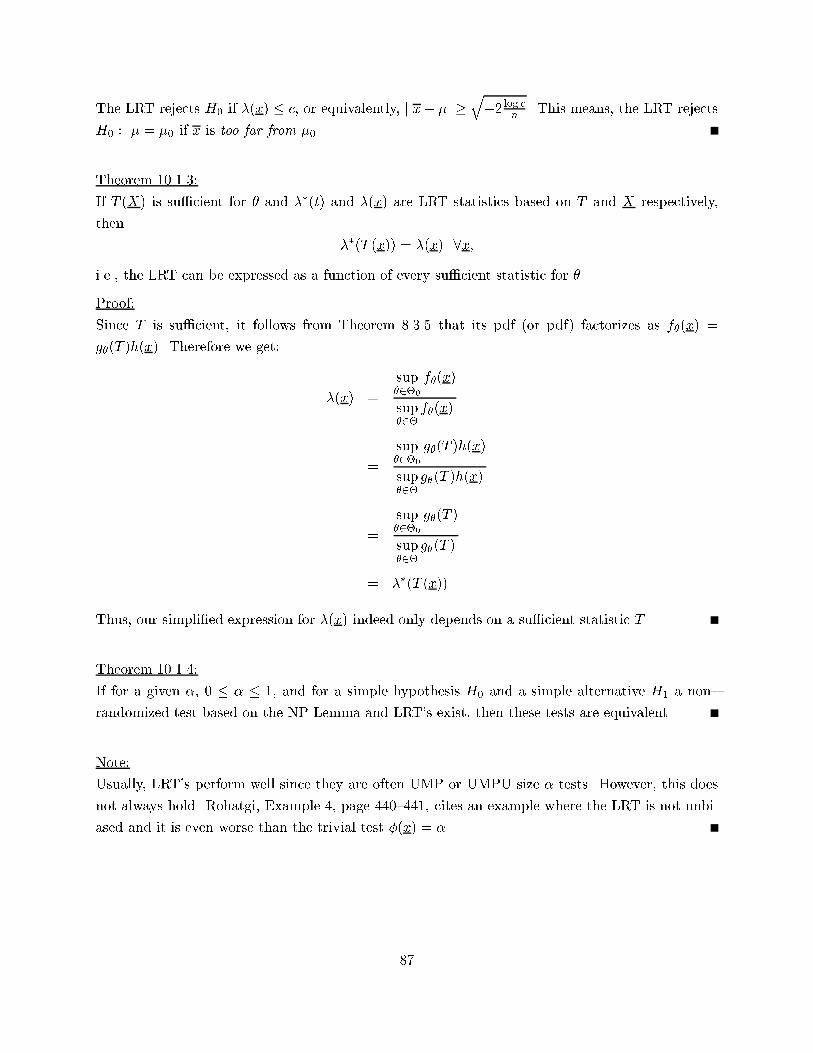
The LRT rejects H0 if �(x) � c, or equivalently, j x� � j�q�2 log c
n. This means, the LRT rejects
H0 : � = �0 if x is too far from �0.
Theorem 10.1.3:
If T (X) is su�cient for � and ��(t) and �(x) are LRT statistics based on T and X respectively,
then
��(T (x)) = �(x) 8x;
i.e., the LRT can be expressed as a function of every su�cient statistic for �.
Proof:
Since T is su�cient, it follows from Theorem 8.3.5 that its pdf (or pdf) factorizes as f�(x) =
g�(T )h(x). Therefore we get:
�(x) =
sup�2�0
f�(x)
sup�2�
f�(x)
=
sup�2�0
g�(T )h(x)
sup�2�
g�(T )h(x)
=
sup�2�0
g�(T )
sup�2�
g�(T )
= ��(T (x))
Thus, our simpli�ed expression for �(x) indeed only depends on a su�cient statistic T .
Theorem 10.1.4:
If for a given �, 0 � � � 1, and for a simple hypothesis H0 and a simple alternative H1 a non{
randomized test based on the NP Lemma and LRT's exist, then these tests are equivalent.
Note:
Usually, LRT's perform well since they are often UMP or UMPU size � tests. However, this does
not always hold. Rohatgi, Example 4, page 440{441, cites an example where the LRT is not unbi-
ased and it is even worse than the trivial test �(x) = �.
87
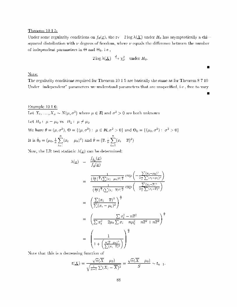
Theorem 10.1.5:
Under some regularity conditions on f�(x), the rv �2 log �(X) under H0 has asymptotically a chi{
squared distribution with � degrees of freedom, where � equals the di�erence between the number
of independent parameters in � and �0, i.e.,
�2 log �(X)d�! �2� under H0:
Note:
The regularity conditions required for Theorem 10.1.5 are basically the same as for Theorem 8.7.10.
Under \independent" parameters we understand parameters that are unspeci�ed, i.e., free to vary.
Example 10.1.6:
Let X1; : : : ; Xn � N(�; �2) where � 2 IR and �2 > 0 are both unknown.
Let H0 : � = �0 vs. H1 : � 6= �0.
We have � = (�; �2), � = f(�; �2) : � 2 IR; �2 > 0g and �0 = f(�0; �2) : �2 > 0g.
It is �̂0 = (�0;1n
nXi=1
(xi � �0)2) and �̂ = (x; 1
n
nXi=1
(xi � x)2).
Now, the LR test statistic �(x) can be determined:
�(x) =f�̂0(x)
f�̂(x)
=
1
( 2�n )n2 (P
(xi��0)2)n2
exp
��
P(xi��0)2
2 1n
P(xi��0)2
�1
( 2�n )n2 (P
(xi�x)2)n2
exp
��
P(xi�x)2
2 1n
P(xi�x)2
�
=
P(xi � x)2P(xi � �0)2
!n2
=
Px2i� nx2P
x2i� 2�0
Pxi + n�20 � nx2 + nx2
!n2
=
0BB@ 1
1 +
�n(x��0)2P(xi�x)2
�1CCA
n2
Note that this is a decreasing function of
t(X) =
pn(X � �0)q
1n�1
P(Xi �X)2
=
pn(X � �0)
S� tn�1:
88
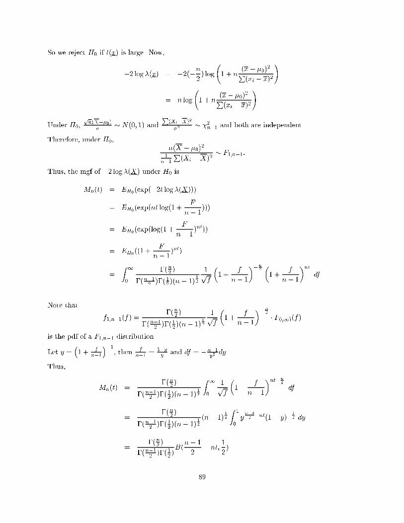
So we reject H0 if t(x) is large. Now,
�2 log �(x) = �2(�n2) log
1 + n
(x� �0)2P
(xi � x)2
!
= n log
1 + n
(x� �0)2P
(xi � x)2
!
Under H0,pn(X��0)
�� N(0; 1) and
P(Xi�X)2
�2� �2
n�1 and both are independent.
Therefore, under H0,n(X � �0)
2
1n�1
P(Xi �X)2
� F1;n�1:
Thus, the mgf of �2 log �(X) under H0 is
Mn(t) = EH0(exp(�2t log �(X)))
= EH0(exp(nt log(1 +
F
n� 1)))
= EH0(exp(log(1 +
F
n� 1)nt))
= EH0((1 +
F
n� 1)nt)
=
Z 1
0
�(n2 )
�(n�12 )�(12)(n� 1)12
1pf
�1 +
f
n� 1
��n2�1 +
f
n� 1
�ntdf
Note that
f1;n�1(f) =�(n2 )
�(n�12 )�(12 )(n� 1)12
1pf
�1 +
f
n� 1
��n2
� I[0;1)(f)
is the pdf of a F1;n�1 distribution.
Let y =�1 + f
n�1
��1, then f
n�1 =1�yy
and df = �n�1y2dy.
Thus,
Mn(t) =�(n2 )
�(n�12 )�(12)(n� 1)12
Z 1
0
1pf
�1 +
f
n� 1
�nt�n2
df
=�(n2 )
�(n�12 )�(12)(n� 1)12
(n� 1)12
Z 1
0yn�32�nt(1� y)�
12 dy
=�(n2 )
�(n�12 )�(12)B(
n� 1
2� nt;
1
2)
89
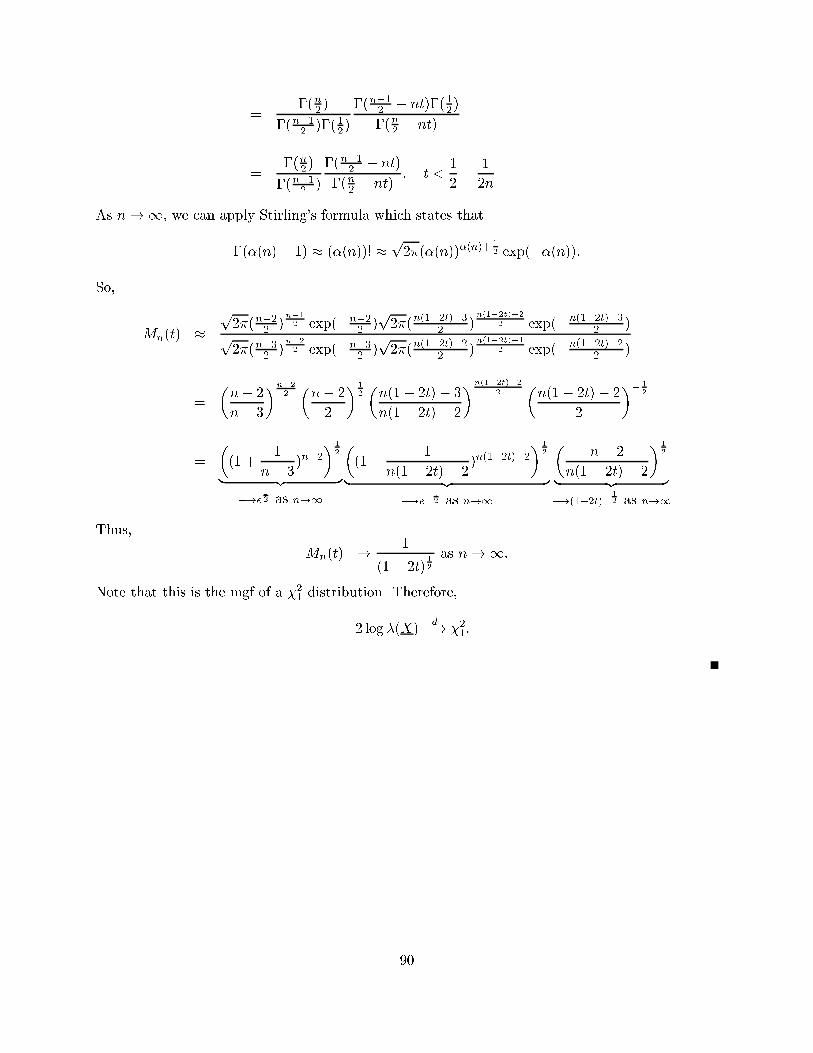
=�(n2 )
�(n�12 )�(12)
�(n�12 � nt)�(12)
�(n2 � nt)
=�(n
2)
�(n�12 )
�(n�12� nt)
�(n2� nt)
; t <1
2� 1
2n
As n!1, we can apply Stirling's formula which states that
�(�(n) + 1) � (�(n))! �p2�(�(n))�(n)+
12 exp(��(n)):
So,
Mn(t) �p2�(n�22 )
n�12 exp(�n�2
2 )p2�(
n(1�2t)�32 )
n(1�2t)�2
2 exp(�n(1�2t)�32 )
p2�(n�32 )
n�22 exp(�n�3
2 )p2�(
n(1�2t)�22 )
n(1�2t)�1
2 exp(�n(1�2t)�22 )
=
�n� 2
n� 3
�n�22�n� 2
2
� 12�n(1� 2t)� 3
n(1� 2t)� 2
�n(1�2t)�2
2�n(1� 2t)� 2
2
�� 12
=
�(1 +
1
n� 3)n�2
� 12
| {z }�!e
12 as n!1
�(1� 1
n(1� 2t)� 2)n(1�2t)�2
� 12
| {z }�!e
�12 as n!1
�n� 2
n(1� 2t)� 2
� 12
| {z }�!(1�2t)�
12 as n!1
Thus,
Mn(t) �!1
(1� 2t)12
as n!1:
Note that this is the mgf of a �21 distribution. Therefore,
�2 log �(X)d�! �21:
90
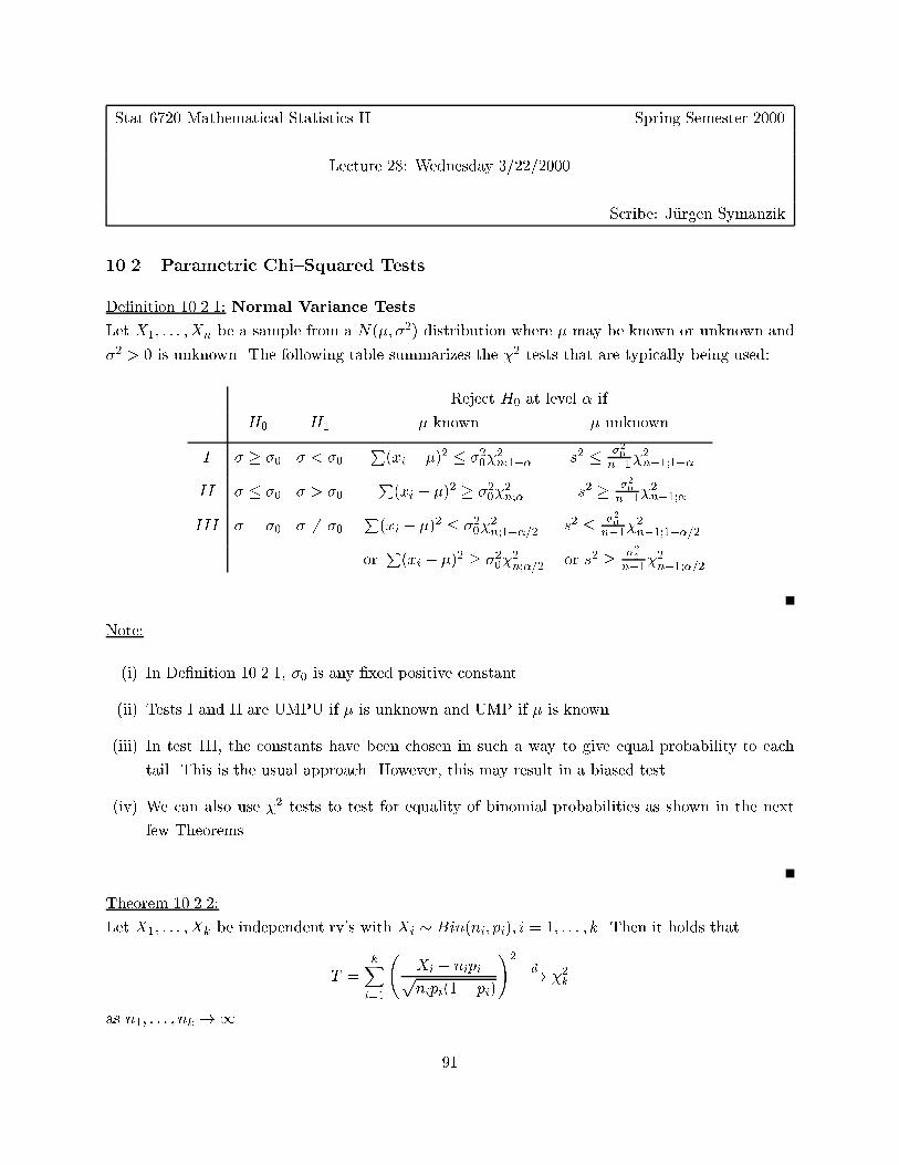
Stat 6720 Mathematical Statistics II Spring Semester 2000
Lecture 28: Wednesday 3/22/2000
Scribe: J�urgen Symanzik
10.2 Parametric Chi{Squared Tests
De�nition 10.2.1: Normal Variance Tests
Let X1; : : : ; Xn be a sample from a N(�; �2) distribution where � may be known or unknown and
�2 > 0 is unknown. The following table summarizes the �2 tests that are typically being used:
Reject H0 at level � if
H0 H1 � known � unknown
I � � �0 � < �0P(xi � �)2 � �20�
2n;1�� s2 � �20
n�1�2n�1;1��
II � � �0 � > �0P(xi � �)2 � �20�
2n;� s2 � �
20
n�1�2n�1;�
III � = �0 � 6= �0P(xi � �)2 � �20�
2n;1��=2 s2 � �
20
n�1�2n�1;1��=2
orP(xi � �)2 � �20�
2n;�=2 or s2 � �
20
n�1�2n�1;�=2
Note:
(i) In De�nition 10.2.1, �0 is any �xed positive constant.
(ii) Tests I and II are UMPU if � is unknown and UMP if � is known.
(iii) In test III, the constants have been chosen in such a way to give equal probability to each
tail. This is the usual approach. However, this may result in a biased test.
(iv) We can also use �2 tests to test for equality of binomial probabilities as shown in the next
few Theorems.
Theorem 10.2.2:
Let X1; : : : ; Xk be independent rv's with Xi � Bin(ni; pi); i = 1; : : : ; k. Then it holds that
T =kXi=1
Xi � nipipnipi(1� pi)
!2d�! �2k
as n1; : : : ; nk !1.
91
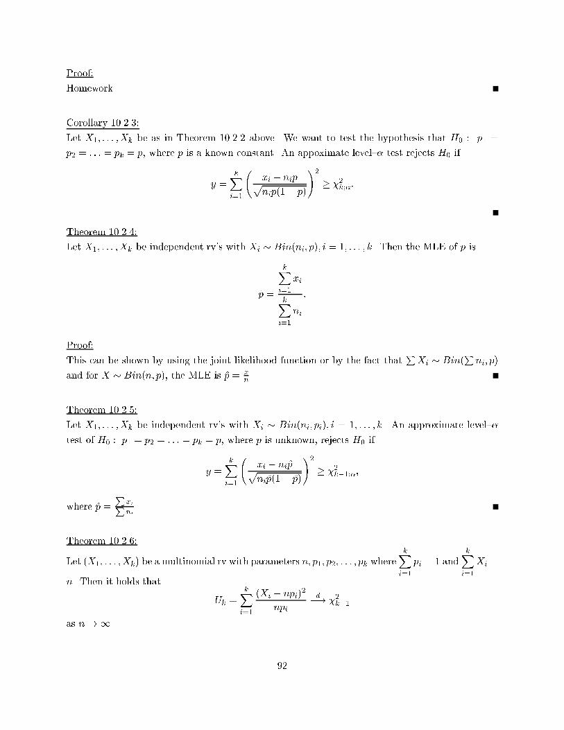
Proof:
Homework
Corollary 10.2.3:
Let X1; : : : ;Xk be as in Theorem 10.2.2 above. We want to test the hypothesis that H0 : p1 =
p2 = : : : = pk = p, where p is a known constant. An appoximate level{� test rejects H0 if
y =kXi=1
xi � nippnip(1� p)
!2
� �2k;�:
Theorem 10.2.4:
Let X1; : : : ; Xk be independent rv's with Xi � Bin(ni; p); i = 1; : : : ; k. Then the MLE of p is
p̂ =
kXi=1
xi
kXi=1
ni
:
Proof:
This can be shown by using the joint likelihood function or by the fact thatPXi � Bin(
Pni; p)
and for X � Bin(n; p), the MLE is p̂ = x
n.
Theorem 10.2.5:
Let X1; : : : ;Xk be independent rv's with Xi � Bin(ni; pi); i = 1; : : : ; k. An approximate level{�
test of H0 : p1 = p2 = : : : = pk = p, where p is unknown, rejects H0 if
y =kXi=1
xi � nip̂pnip̂(1� p̂)
!2
� �2k�1;�;
where p̂ =
PxiPni.
Theorem 10.2.6:
Let (X1; : : : ;Xk) be a multinomial rv with parameters n; p1; p2; : : : ; pk wherekXi=1
pi = 1 andkXi=1
Xi =
n. Then it holds that
Uk =kXi=1
(Xi � npi)2
npi
d�! �2k�1
as n!1.
92
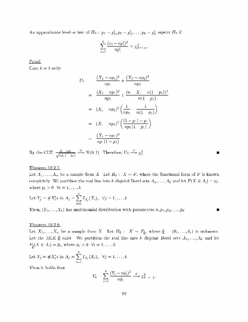
An approximate level{� test of H0 : p1 = p01; p2 = p02; : : : ; pk = p0krejects H0 if
kXi=1
(xi � np0i)2
np0i
> �2k�1;�:
Proof:
Case k = 2 only:
U2 =(X1 � np1)
2
np1+(X2 � np2)
2
np2
=(X1 � np1)
2
np1+(n�X1 � n(1� p1))
2
n(1� p1)
= (X1 � np1)2
�1
np1+
1
n(1� p1)
�
= (X1 � np1)2
�(1� p1) + p1
np1(1� p1)
�
=(X1 � np1)
2
np1(1� p1)
By the CLT, X1�np1pnp1(1�p1)
d�! N(0; 1). Therefore, U2d�! �21.
Theorem 10.2.7:
Let X1; : : : ;Xn be a sample from X. Let H0 : X � F , where the functional form of F is known
completely. We partition the real line into k disjoint Borel sets A1; : : : ; Ak and let P (X 2 Ai) = pi,
where pi > 0 8i = 1; : : : ; k.
Let Yj = #X 0is in Aj =
nXi=1
IAj (Xi); 8j = 1; : : : ; k.
Then, (Y1; : : : ; Yk) has multinomial distribution with parameters n; p1; p2; : : : ; pk.
Theorem 10.2.8:
Let X1; : : : ;Xn be a sample from X. Let H0 : X � F�, where � = (�1; : : : ; �r) is unknown.
Let the MLE �̂ exist. We partition the real line into k disjoint Borel sets A1; : : : ; Ak and let
P�̂(X 2 Ai) = p̂i, where p̂i > 0 8i = 1; : : : ; k.
Let Yj = #X 0is in Aj =
nXi=1
IAj (Xi); 8j = 1; : : : ; k.
Then it holds that
Vk =kXi=1
(Yi � np̂i)2
np̂i
d�! �2k�r�1:
93
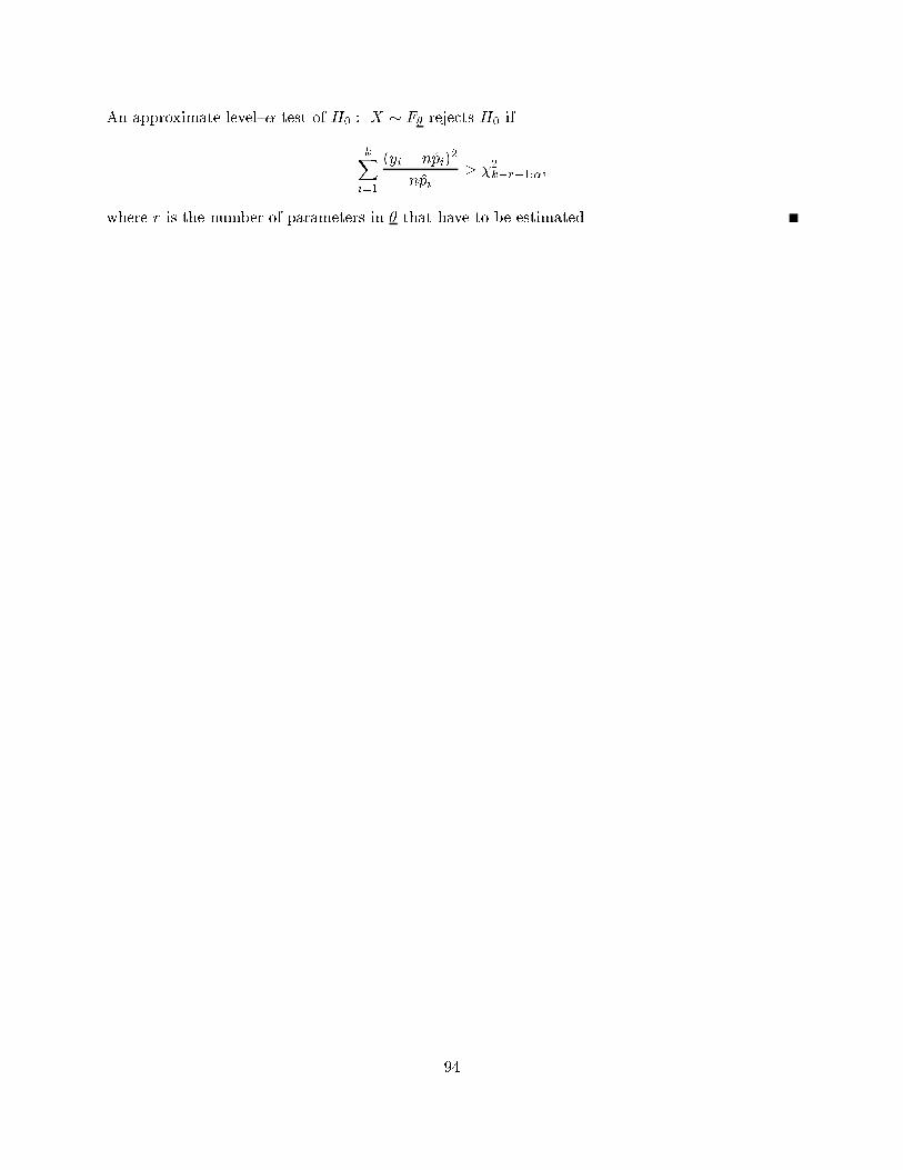
An approximate level{� test of H0 : X � F� rejects H0 if
kXi=1
(yi � np̂i)2
np̂i> �2k�r�1;�;
where r is the number of parameters in � that have to be estimated.
94
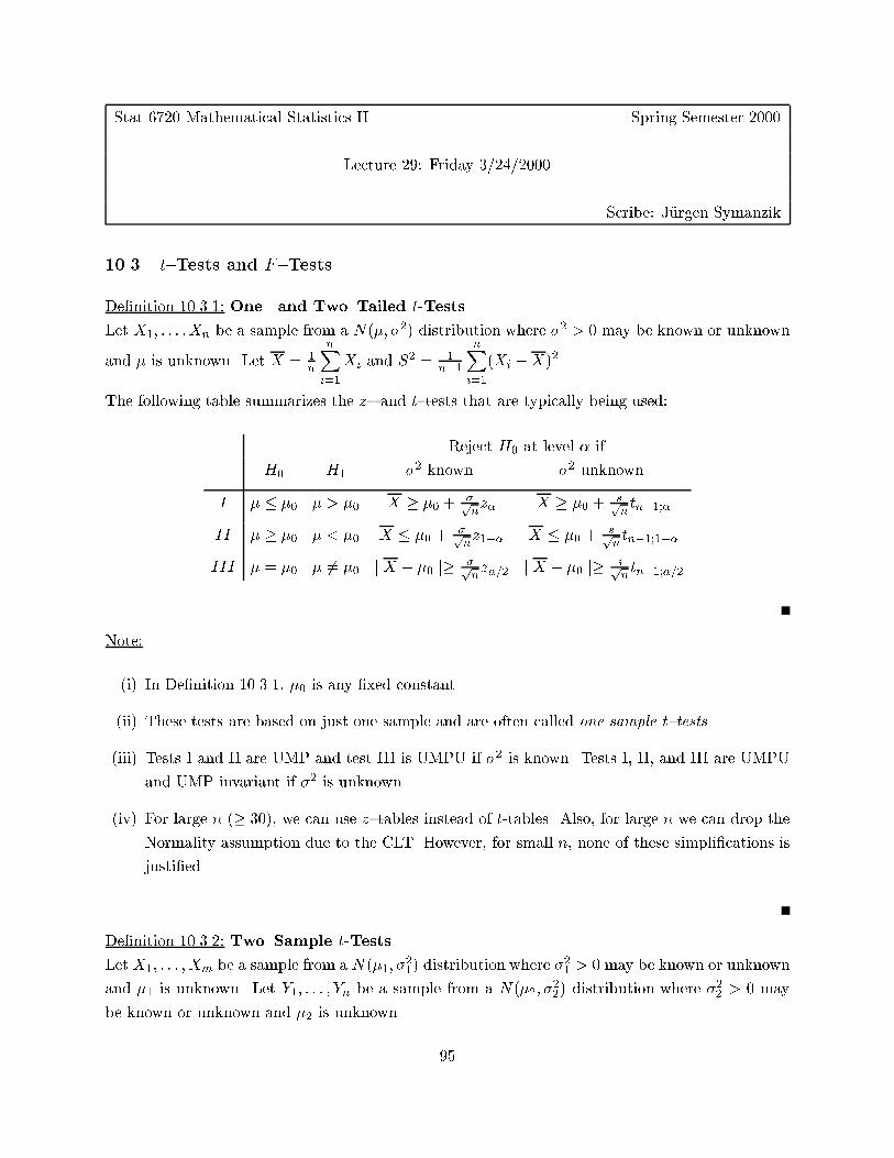
Stat 6720 Mathematical Statistics II Spring Semester 2000
Lecture 29: Friday 3/24/2000
Scribe: J�urgen Symanzik
10.3 t{Tests and F{Tests
De�nition 10.3.1: One{ and Two{Tailed t-Tests
Let X1; : : : ;Xn be a sample from a N(�; �2) distribution where �2 > 0 may be known or unknown
and � is unknown. Let X = 1n
nXi=1
Xi and S2 = 1
n�1
nXi=1
(Xi �X)2.
The following table summarizes the z{ and t{tests that are typically being used:
Reject H0 at level � if
H0 H1 �2 known �2 unknown
I � � �0 � > �0 X � �0 +�pnz� X � �0 +
spntn�1;�
II � � �0 � < �0 X � �0 +�pnz1�� X � �0 +
spntn�1;1��
III � = �0 � 6= �0 j X � �0 j� �pnz�=2 j X � �0 j� sp
ntn�1;�=2
Note:
(i) In De�nition 10.3.1, �0 is any �xed constant.
(ii) These tests are based on just one sample and are often called one sample t{tests.
(iii) Tests I and II are UMP and test III is UMPU if �2 is known. Tests I, II, and III are UMPU
and UMP invariant if �2 is unknown.
(iv) For large n (� 30), we can use z{tables instead of t-tables. Also, for large n we can drop the
Normality assumption due to the CLT. However, for small n, none of these simpli�cations is
justi�ed.
De�nition 10.3.2: Two{Sample t-Tests
Let X1; : : : ;Xm be a sample from a N(�1; �21) distribution where �
21 > 0 may be known or unknown
and �1 is unknown. Let Y1; : : : ; Yn be a sample from a N(�2; �22) distribution where �22 > 0 may
be known or unknown and �2 is unknown.
95
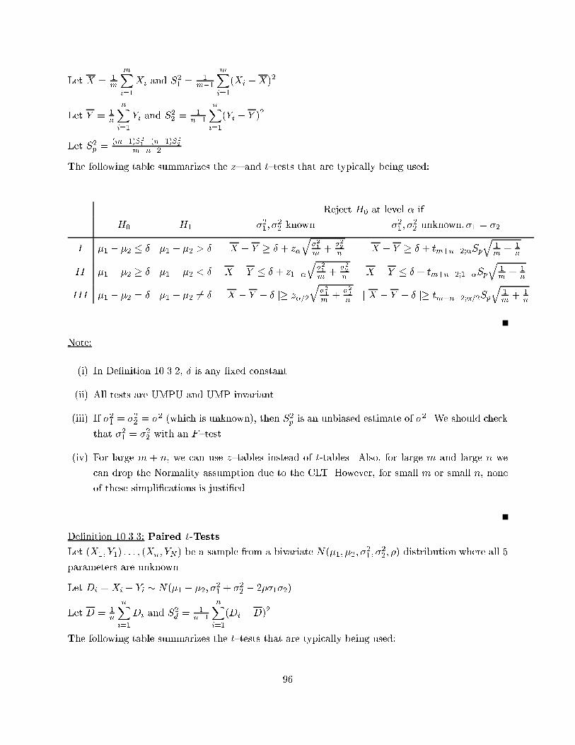
Let X = 1m
mXi=1
Xi and S21 =
1m�1
mXi=1
(Xi �X)2.
Let Y = 1n
nXi=1
Yi and S22 =
1n�1
nXi=1
(Yi � Y )2.
Let S2p =(m�1)S21+(n�1)S22
m+n�2 .
The following table summarizes the z{ and t{tests that are typically being used:
Reject H0 at level � if
H0 H1 �21; �22 known �21 ; �
22 unknown; �1 = �2
I �1 � �2 � � �1 � �2 > � X � Y � � + z�
q�21
m+
�22
nX � Y � � + tm+n�2;�Sp
q1m+ 1
n
II �1 � �2 � � �1 � �2 < � X � Y � � + z1��
q�21
m+
�22
nX � Y � � + tm+n�2;1��Sp
q1m+ 1
n
III �1 � �2 = � �1 � �2 6= � j X � Y � � j� z�=2
q�21
m+
�22
nj X � Y � � j� tm+n�2;�=2Sp
q1m+ 1
n
Note:
(i) In De�nition 10.3.2, � is any �xed constant.
(ii) All tests are UMPU and UMP invariant.
(iii) If �21 = �22 = �2 (which is unknown), then S2p is an unbiased estimate of �2. We should check
that �21 = �22 with an F{test.
(iv) For large m + n, we can use z{tables instead of t-tables. Also, for large m and large n we
can drop the Normality assumption due to the CLT. However, for small m or small n, none
of these simpli�cations is justi�ed.
De�nition 10.3.3: Paired t-Tests
Let (X1; Y1) : : : ; (Xn; YN ) be a sample from a bivariate N(�1; �2; �21 ; �
22 ; �) distribution where all 5
parameters are unknown.
Let Di = Xi � Yi � N(�1 � �2; �21 + �22 � 2��1�2).
Let D = 1n
nXi=1
Di and S2d= 1
n�1
nXi=1
(Di �D)2.
The following table summarizes the t{tests that are typically being used:
96
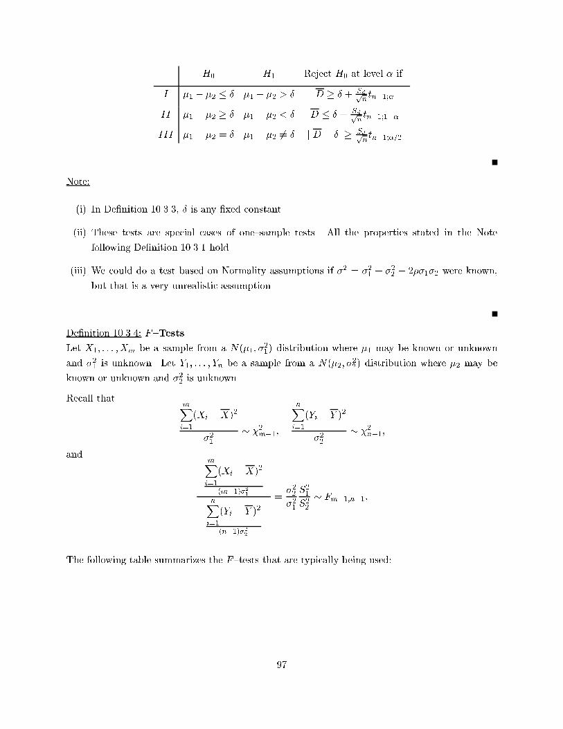
H0 H1 Reject H0 at level � if
I �1 � �2 � � �1 � �2 > � D � � + Sdpntn�1;�
II �1 � �2 � � �1 � �2 < � D � � + Sdpntn�1;1��
III �1 � �2 = � �1 � �2 6= � j D � � j� Sdpntn�1;�=2
Note:
(i) In De�nition 10.3.3, � is any �xed constant.
(ii) These tests are special cases of one{sample tests. All the properties stated in the Note
following De�nition 10.3.1 hold.
(iii) We could do a test based on Normality assumptions if �2 = �21 + �22 � 2��1�2 were known,
but that is a very unrealistic assumption.
De�nition 10.3.4: F{Tests
Let X1; : : : ;Xm be a sample from a N(�1; �21) distribution where �1 may be known or unknown
and �21 is unknown. Let Y1; : : : ; Yn be a sample from a N(�2; �22) distribution where �2 may be
known or unknown and �22 is unknown.
Recall thatmXi=1
(Xi �X)2
�21� �2m�1;
nXi=1
(Yi � Y )2
�22� �2n�1;
andmXi=1
(Xi �X)2
(m�1)�21nXi=1
(Yi � Y )2
(n�1)�22
=�22
�21
S21
S22� Fm�1;n�1:
The following table summarizes the F{tests that are typically being used:
97
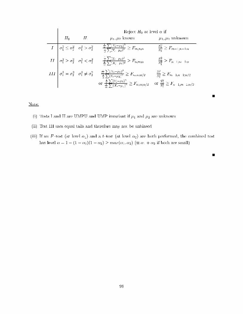
Reject H0 at level � if
H0 H1 �1; �2 known �1; �2 unknown
I �21 � �22 �21 > �22
1m
P(Xi��1)2
1n
P(Yi��2)2
� Fm;n;�S21
S22
� Fm�1;n�1;�
II �21 � �22 �21 < �22
1n
P(Yi��2)2
1m
P(Xi��1)2
� Fn;m;�S22
S21
� Fn�1;m�1;�
III �21 = �22 �21 6= �22
1m
P(Xi��1)2
1n
P(Yi��2)2
� Fm;n;�=2S21
S22
� Fm�1;n�1;�=2
or1n
P(Yi��2)2
1m
P(Xi��1)2
� Fn;m;�=2 orS22
S21
� Fn�1;m�1;�=2
Note:
(i) Tests I and II are UMPU and UMP invariant if �1 and �2 are unknown.
(ii) Test III uses equal tails and therefore may not be unbiased.
(iii) If an F{test (at level �1) and a t{test (at level �2) are both performed, the combined test
has level � = 1� (1� �1)(1 � �2) � max(�1; �2) (� �1 + �2 if both are small).
98
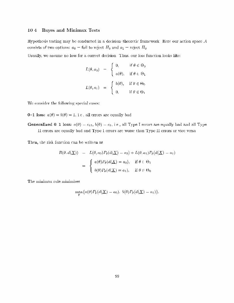
10.4 Bayes and Minimax Tests
Hypothesis testing may be conducted in a decision{theoretic framework. Here our action space A
consists of two options: a0 = fail to reject H0 and a1 = reject H0.
Usually, we assume no loss for a correct decision. Thus, our loss function looks like:
L(�; a0) =
8<: 0; if � 2 �0
a(�); if � 2 �1
L(�; a1) =
8<: b(�); if � 2 �0
0; if � 2 �1
We consider the following special cases:
0{1 loss: a(�) = b(�) = 1, i.e., all errors are equally bad.
Generalized 0{1 loss: a(�) = cII , b(�) = cI , i.e., all Type I errors are equally bad and all Type
II errors are equally bad and Type I errors are worse than Type II errors or vice versa.
Then, the risk function can be written as
R(�; d(X)) = L(�; a0)P�(d(X) = a0) + L(�; a1)P�(d(X) = a1)
=
8<: a(�)P�(d(X) = a0); if � 2 �1
b(�)P�(d(X) = a1); if � 2 �0
The minimax rule minimizes
max�
fa(�)P�(d(X) = a0); b(�)P�(d(X) = a1)g:
99
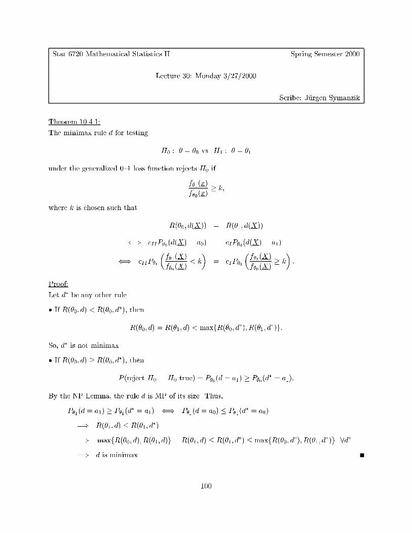
Stat 6720 Mathematical Statistics II Spring Semester 2000
Lecture 30: Monday 3/27/2000
Scribe: J�urgen Symanzik
Theorem 10.4.1:
The minimax rule d for testing
H0 : � = �0 vs. H1 : � = �1
under the generalized 0{1 loss function rejects H0 if
f�1(x)
f�0(x)� k;
where k is chosen such that
R(�0; d(X)) = R(�1; d(X))
() cIIP�1(d(X) = a0) = cIP�0(d(X) = a1)
() cIIP�1
�f�1(X)
f�0(X)< k
�= cIP�0
�f�1(X)
f�0(X)� k
�:
Proof:
Let d� be any other rule.
� If R(�0; d) < R(�0; d�), then
R(�0; d) = R(�1; d) < maxfR(�0; d�); R(�1; d�)g:
So, d� is not minimax.
� If R(�0; d) � R(�0; d�), then
P (reject H0 j H0 true) = P�0(d = a1) � P�0(d� = a1):
By the NP Lemma, the rule d is MP of its size. Thus,
P�1(d = a1) � P�1(d� = a1) () P�1(d = a0) � P�1(d
� = a0)
=) R(�1; d) � R(�1; d�)
=) maxfR(�0; d); R(�1; d)g = R(�1; d) � R(�1; d�) � maxfR(�0; d�); R(�1; d�)g 8d�
=) d is minimax
100
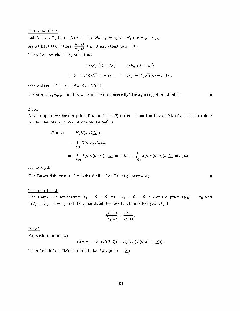
Example 10.4.2:
Let X1; : : : ; Xn be iid N(�; 1). Let H0 : � = �0 vs. H1 : � = �1 > �0.
As we have seen before,f�1
(x)
f�0(x)
� k1 is equivalent to x � k2.
Therefore, we choose k2 such that
cIIP�1(X < k2) = cIP�0(X � k2)
() cII�(pn(k2 � �1)) = cI(1��(
pn(k2 � �0)));
where �(z) = P (Z � z) for Z � N(0; 1).
Given cI ; cII ; �0; �1, and n, we can solve (numerically) for k2 using Normal tables.
Note:
Now suppose we have a prior distribution �(�) on �. Then the Bayes risk of a decision rule d
(under the loss function introduced before) is
R(�; d) = E�R(�; d(X))
=
Z�R(�; d)�(�)d�
=
Z�0
b(�)�(�)P�(d(X) = a1)d� +
Z�1
a(�)�(�)P�(d(X) = a0)d�
if � is a pdf.
The Bayes risk for a pmf � looks similar (see Rohatgi, page 461).
Theorem 10.4.3:
The Bayes rule for testing H0 : � = �0 vs. H1 : � = �1 under the prior �(�0) = �0 and
�(�1) = �1 = 1� �0 and the generalized 0{1 loss function is to reject H0 if
f�1(x)
f�0(x)� cI�0
cII�1:
Proof:
We wish to minimize
R(�; d) = E�(R(�; d)) = E�(E�(L(�; d) j X)):
Therefore, it is su�cient to minimize E�(L(�; d) j X).
101
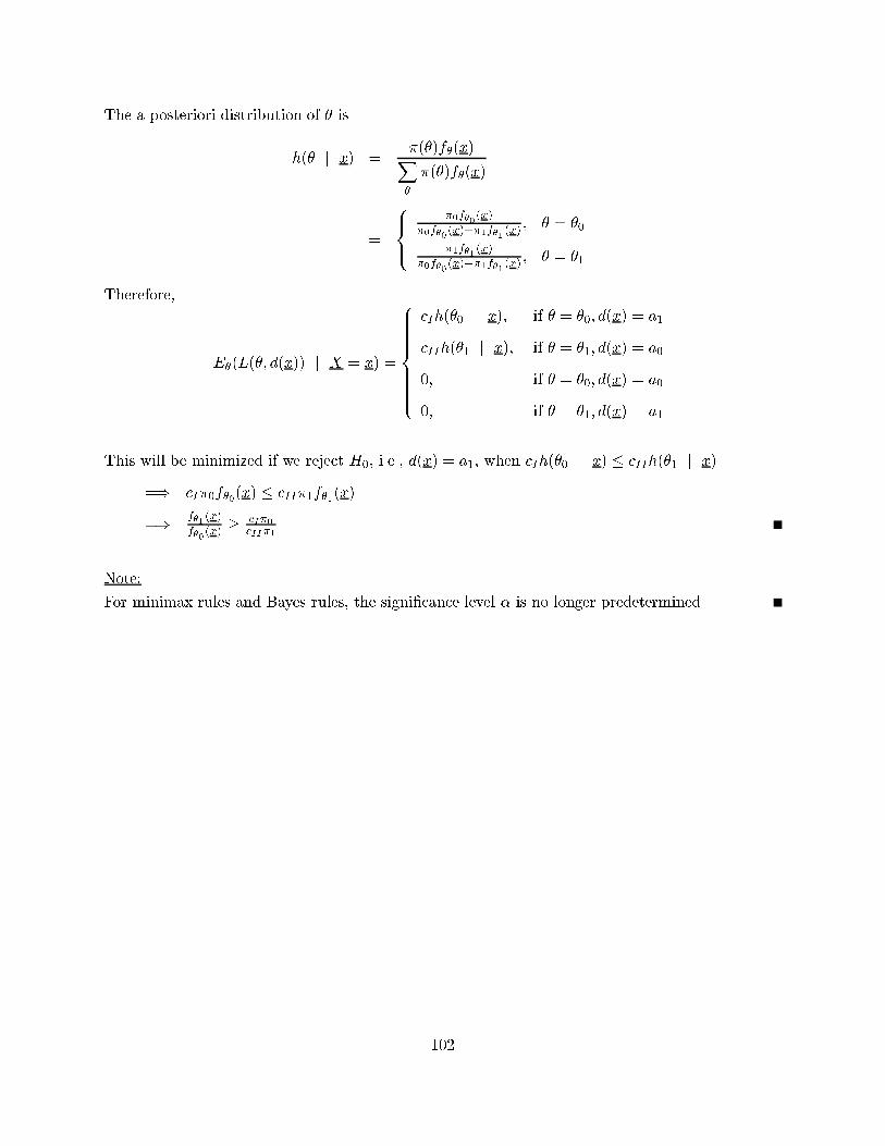
The a posteriori distribution of � is
h(� j x) =�(�)f�(x)X�
�(�)f�(x)
=
8><>:�0f�0
(x)
�0f�0(x)+�1f�1 (x)
; � = �0
�1f�1(x)
�0f�0(x)+�1f�1 (x)
; � = �1
Therefore,
E�(L(�; d(x)) j X = x) =
8>>>>>>><>>>>>>>:
cIh(�0 j x); if � = �0; d(x) = a1
cIIh(�1 j x); if � = �1; d(x) = a0
0; if � = �0; d(x) = a0
0; if � = �1; d(x) = a1
This will be minimized if we reject H0, i.e., d(x) = a1, when cIh(�0 j x) � cIIh(�1 j x)
=) cI�0f�0(x) � cII�1f�1(x)
=) f�1(x)
f�0(x) �
cI�0
cII�1
Note:
For minimax rules and Bayes rules, the signi�cance level � is no longer predetermined.
102
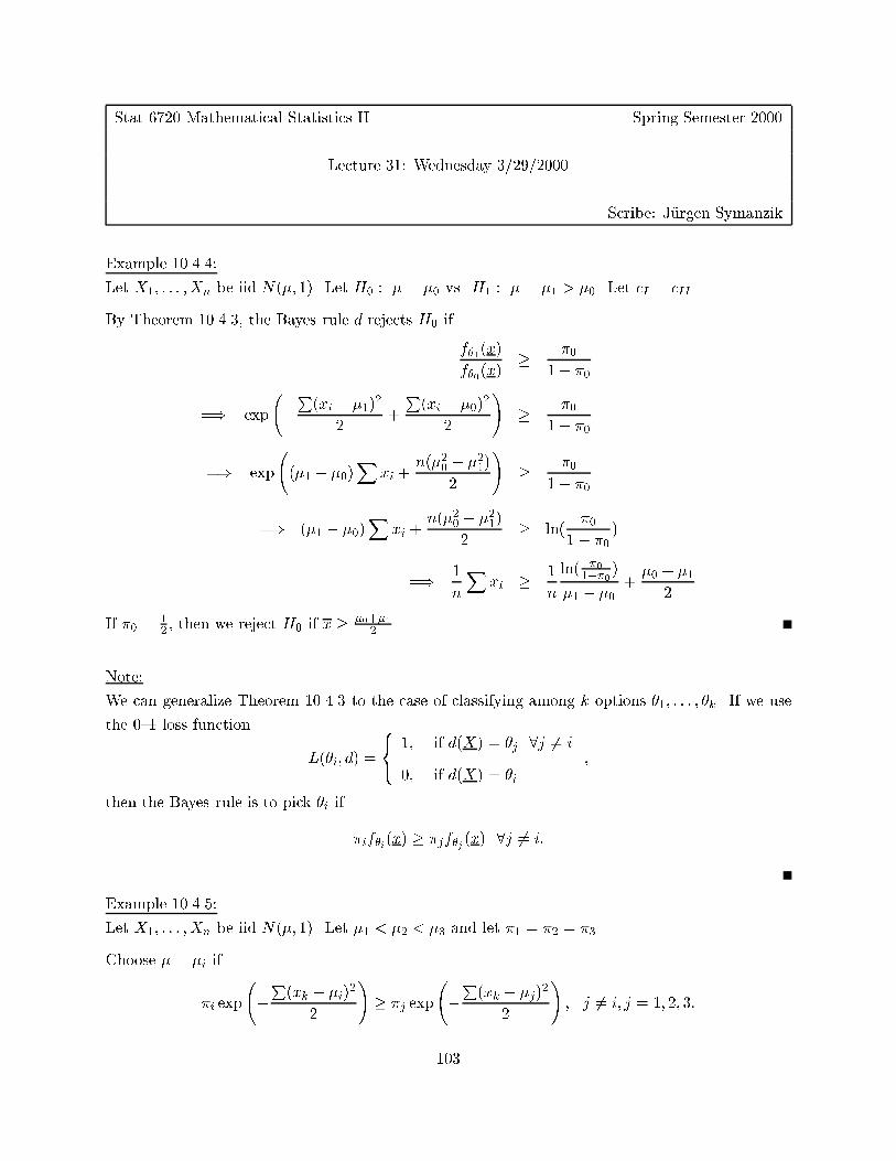
Stat 6720 Mathematical Statistics II Spring Semester 2000
Lecture 31: Wednesday 3/29/2000
Scribe: J�urgen Symanzik
Example 10.4.4:
Let X1; : : : ; Xn be iid N(�; 1). Let H0 : � = �0 vs. H1 : � = �1 > �0. Let cI = cII .
By Theorem 10.4.3, the Bayes rule d rejects H0 if
f�1(x)
f�0(x)� �0
1� �0
=) exp
�P(xi � �1)
2
2+
P(xi � �0)
2
2
!� �0
1� �0
=) exp
(�1 � �0)
Xxi +
n(�20 � �21)
2
!� �0
1� �0
=) (�1 � �0)X
xi +n(�20 � �21)
2� ln(
�0
1� �0)
=) 1
n
Xxi � 1
n
ln( �0
1��0 )
�1 � �0+�0 + �1
2
If �0 =12 , then we reject H0 if x � �0+�1
2 .
Note:
We can generalize Theorem 10.4.3 to the case of classifying among k options �1; : : : ; �k. If we use
the 0{1 loss function
L(�i; d) =
8<: 1; if d(X) = �j 8j 6= i
0; if d(X) = �i
;
then the Bayes rule is to pick �i if
�if�i(x) � �jf�j (x) 8j 6= i:
Example 10.4.5:
Let X1; : : : ; Xn be iid N(�; 1). Let �1 < �2 < �3 and let �1 = �2 = �3.
Choose � = �i if
�i exp
�P(xk � �i)
2
2
!� �j exp
�P(xk � �j)
2
2
!; j 6= i; j = 1; 2; 3:
103

Similar to Example 10.4.4, these conditions can be transformed as follows:
x(�i � �j) �(�i � �j)(�i + �j)
2; j 6= i; j = 1; 2; 3:
In our particular example, we get the following decision rules:
(i) Choose �1 if x � �1+�22 (and x � �1+�3
2 ).
(ii) Choose �2 if x � �1+�22 and x � �2+�3
2 .
(iii) Choose �3 if x � �2+�32
(and x � �1+�32
).
Note that in (i) and (iii) the condition in parentheses automatically holds when the other condition
holds.
If �1 = 0; �2 = 2, and �3 = 4, we have the decision rules:
(i) Choose �1 if x � 1.
(ii) Choose �2 if 1 � x � 3.
(iii) Choose �3 if x � 3.
We do not have to worry how to handle the boundary since the probability that the rv will realize
on any of the two boundary points is 0.
104
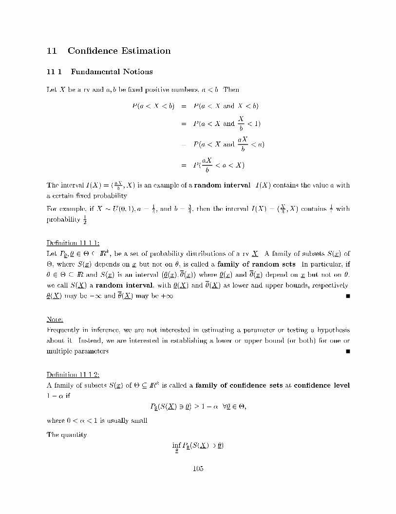
11 Con�dence Estimation
11.1 Fundamental Notions
Let X be a rv and a; b be �xed positive numbers, a < b. Then
P (a < X < b) = P (a < X and X < b)
= P (a < X andX
b< 1)
= P (a < X andaX
b< a)
= P (aX
b< a < X)
The interval I(X) = (aXb; X) is an example of a random interval. I(X) contains the value a with
a certain �xed probability.
For example, if X � U(0; 1); a = 14 , and b =
34 , then the interval I(X) = (X3 ;X) contains 1
4 with
probability 12 .
De�nition 11.1.1:
Let P�; � 2 � � IRk, be a set of probability distributions of a rv X. A family of subsets S(x) of
�, where S(x) depends on x but not on �, is called a family of random sets. In particular, if
� 2 � � IR and S(x) is an interval (�(x); �(x)) where �(x) and �(x) depend on x but not on �,
we call S(X) a random interval, with �(X) and �(X) as lower and upper bounds, respectively.
�(X) may be �1 and �(X) may be +1.
Note:
Frequently in inference, we are not interested in estimating a parameter or testing a hypothesis
about it. Instead, we are interested in establishing a lower or upper bound (or both) for one or
multiple parameters.
De�nition 11.1.2:
A family of subsets S(x) of � � IRk is called a family of con�dence sets at con�dence level
1� � if
P�(S(X) 3 �) � 1� � 8� 2 �;
where 0 < � < 1 is usually small.
The quantity
inf�
P�(S(X) 3 �)
105
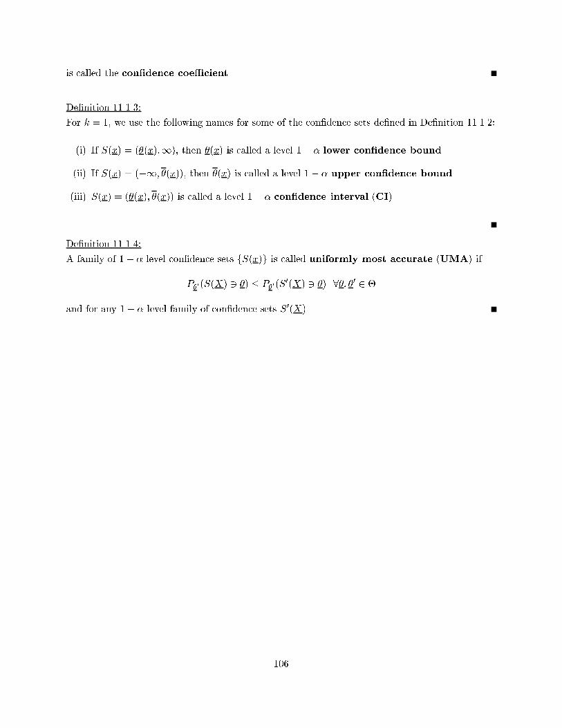
is called the con�dence coe�cient.
De�nition 11.1.3:
For k = 1, we use the following names for some of the con�dence sets de�ned in De�nition 11.1.2:
(i) If S(x) = (�(x);1), then �(x) is called a level 1� � lower con�dence bound.
(ii) If S(x) = (�1; �(x)), then �(x) is called a level 1� � upper con�dence bound.
(iii) S(x) = (�(x); �(x)) is called a level 1� � con�dence interval (CI).
De�nition 11.1.4:
A family of 1� � level con�dence sets fS(x)g is called uniformly most accurate (UMA) if
P�0(S(X) 3 �) � P�0(S0(X) 3 �) 8�; �0 2 �
and for any 1� � level family of con�dence sets S0(X).
106
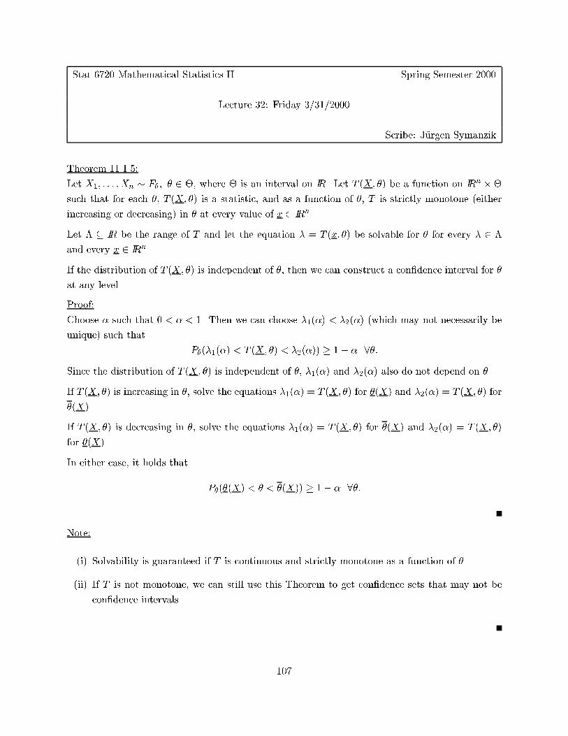
Stat 6720 Mathematical Statistics II Spring Semester 2000
Lecture 32: Friday 3/31/2000
Scribe: J�urgen Symanzik
Theorem 11.1.5:
Let X1; : : : ;Xn � F�; � 2 �, where � is an interval on IR. Let T (X; �) be a function on IRn ��
such that for each �, T (X; �) is a statistic, and as a function of �, T is strictly monotone (either
increasing or decreasing) in � at every value of x 2 IRn.
Let � � IR be the range of T and let the equation � = T (x; �) be solvable for � for every � 2 �
and every x 2 IRn.
If the distribution of T (X; �) is independent of �, then we can construct a con�dence interval for �
at any level.
Proof:
Choose � such that 0 < � < 1. Then we can choose �1(�) < �2(�) (which may not necessarily be
unique) such that
P�(�1(�) < T (X; �) < �2(�)) � 1� � 8�:
Since the distribution of T (X; �) is independent of �, �1(�) and �2(�) also do not depend on �.
If T (X; �) is increasing in �, solve the equations �1(�) = T (X; �) for �(X) and �2(�) = T (X; �) for
�(X).
If T (X; �) is decreasing in �, solve the equations �1(�) = T (X; �) for �(X) and �2(�) = T (X; �)
for �(X).
In either case, it holds that
P�(�(X) < � < �(X)) � 1� � 8�:
Note:
(i) Solvability is guaranteed if T is continuous and strictly monotone as a function of �.
(ii) If T is not monotone, we can still use this Theorem to get con�dence sets that may not be
con�dence intervals.
107
Example 11.1.6:
Let X1; : : : ; Xn � N(�; �2), where � and �2 > 0 are both unknown. We seek a 1�� level con�dence
interval for �.
Note that
T (X;�) =X � �
S=pn� tn�1
is independent of � and monotone and decreasing in �.
We choose �1(�) and �2(�) such that
P (�1(�) < T (X;�) < �2(�)) = 1� �
and solve for � which yields
P (X � S�2(�)pn
< � < X � S�1(�)pn
) = 1� �:
Thus,
(X � S�2(�)pn
;X � S�1(�)pn
)
is a 1� � level CI for �. We commonly choose �2(�) = ��1(�) = tn�1;�=2.
Example 11.1.7:
Let X1; : : : ; Xn � U(0; �).
We know that �̂ = max(X(i)) =Maxn is the MLE for � and su�cient for �.
The pdf of Maxn is given by
fn(y) =nyn�1
�nI(0;�)(y):
Then the rv Tn =Maxn
�has the pdf
hn(t) = ntn�1I(0;1)(t);
which is independent of �. Tn is monotone and decreasing in �.
We now have to �nd numbers �1(�) and �2(�) such that
P (�1(�) < Tn < �2(�)) = 1� �
=) n
Zb
a
tn�1dt = 1� �
=) �n2 � �n1 = 1� �
If we choose �2 = 1 and �1 = �1=n, then (Maxn; ��1=nMaxn) is a 1� � level CI for �.
108
11.2 Shortest{Length Con�dence Intervals
In practice, we usually want not only an interval with coverage probability 1 � � for �, but if
possible the shortest (most precise) such interval.
De�nition 11.2.1:
A rv T (X; �) whose distribution is independent of � is called a pivot.
Note:
The methods we will discuss here can provide the shortest interval based on a given pivot. They
will not guarantee that there is no other pivot with a shorter minimal interval.
Example 11.2.2:
Let X1; : : : ; Xn � N(�; �2), where �2 is known. The obvious pivot for � is
T�(X) =X � �
�=pn� N(0; 1):
Suppose that (a; b) is an interval such that P (a < Z < b) = 1� �, where Z � N(0; 1).
A 1� � level CI based on this pivot is found by
1� � = P (a <X � �
�=pn< b) = P (X � b
�pn< � < X � a
�pn):
The length of the interval is L = (b� a) �pn.
To minimize L, we must choose a and b such that b� a is minimal while
�(b)� �(a) =1p2�
Zb
a
e�x2
2 dx = 1� �;
where �(z) = P (Z � z).
To �nd a minimum, we can di�erentiate these expressions with respect to a. However, b is not a
constant but is an implicit function of a. Formally, we could writed b(a)da
. However, this is usually
shortened to db
da.
Here we getd
da(�(b)� �(a)) = �(b)
db
da� �(a) = 0
anddL
da=
�pn(db
da� 1) =
�pn(�(a)
�(b)� 1):
109
The minimum occurs when �(a) = �(b) which happens when a = b or a = �b. If we select a = b,
then �(b)� �(a) = �(a)� �(a) = 0 6= 1 � �. Thus, we must have that b = �a = z�=2. Thus, the
shortest CI based on T� is
(X � z�=2�pn;X + z�=2
�pn):
110
Stat 6720 Mathematical Statistics II Spring Semester 2000
Lecture 33: Monday 4/3/2000
Scribe: J�urgen Symanzik
De�nition 11.2.3:
A pdf f(x) is unimodal i� there exists a x� such that f(x) is nondecreasing for x � x� and f(x)
is nonincreasing for x � x�.
Theorem 11.2.4:
Let f(x) be a unimodal pdf. If the interval [a; b] satis�es
(i)
Zb
a
f(x)dx = 1� �
(ii) f(a) = f(b) > 0, and
(iii) a � x� � b, where x� is a mode of f(x),
then the interval [a; b] is the shortest of all intervals which satisfy condition (i).
Proof:
Let [a0; b0] be any interval with b0 � a0 < b� a. We will show that this implies
Zb
a
f(x)dx < 1� �,
i.e., a contradiction.
We assume that a0 � a. The case a < a0 is similar.
� Suppose that b0 � a. Then a0 � b0 � a � x�. It followsZb0
a0f(x)dx � f(b0)(b0 � a0) jx � b0 � x� ) f(x) � f(b0)
� f(a)(b0 � a0) jb0 � a � x� ) f(b0) < f(a)
< f(a)(b� a) jb0 � a0 < b� a and f(a) > 0
�Zb
a
f(x)dx jf(x) � f(a) for a � x � b
= 1� � jby (i)
� Suppose b0 > a. We can immediately exclude that b0 > b since then b0 � a0 > b � a, i.e., b0 � a0
wouldn't be of shorter length than b� a. Thus, we have to consider the case that a0 � a < b0 < b.
It holds that Zb0
a0f(x)dx =
Zb
a
f(x)dx+
Za
a0f(x)dx�
Zb
b0f(x)dx
111
Note that
Za
a0f(x)dx � f(a)(a� a0) and
Zb
b0f(x)dx � f(b)(b� b0). Therefore, we get
Za
a0�Zb
b0� f(a)(a� a0)� f(b)(b� b0)
= f(a)((a� a0)� (b� b0)) since f(a) = f(b)
= f(a)((b0 � a0)� (b� a))
< 0
Thus, Zb0
a0f(x)dx < a� �:
Note:
Example 11.2.2 is a special case of Theorem 11.2.4.
Example 11.2.5:
Let X1; : : : ; Xn � N(�; �2), where � is known. The obvious pivot for �2 is
T�2(X) =
P(Xi � �)2
�2� �2n:
So
P
a <
P(Xi � �)2
�2< b
!= 1� �
() P
P(Xi � �)2
b< �2 <
P(Xi � �)2
a
!= 1� �
We wish to minimize
L = (1
a� 1
b)X
(Xi � �)2
such that
Zb
a
fn(t)dt = 1� �, where fn(t) is the pdf of a �2n distribution.
We get
fn(b)db
da� fn(a) = 0
anddL
da=
�1
a2� 1
b2db
da
�X(Xi � �)2 =
�1
a2� 1
b2fn(a)
fn(b)
�X(Xi � �)2:
We obtain a minimum if a2fn(a) = b2fn(b).
112
Note that in practice equal tails �2n;�=2 and �
2n;1��=2 are used, which do not result in shortest{length
CI's. The reason for this selection is simple: When these tests were developed, computers did not
exist that could solve these equations numerically. People in general had to rely on tabulated val-
ues. Manually solving the equation above for each case obviously wasn't a feasible solution.
Example 11.2.6:
Let X1; : : : ;Xn � U(0; �). Let Maxn = maxXi = X(n). Since Tn = Maxn
�has pdf ntn�1I(0;1)(t)
which does not depend on �, Tn can be selected as a our pivot. The density of Tn is strictly
increasing for n � 2, so we cannot �nd constants a and b as in Example 11.2.5.
If P (a < Tn < b) = 1� �, then P (Maxn
b< � < Maxn
a) = 1� �.
We wish to minimize
L =Maxn(1
a� 1
b)
such that
Zb
a
ntn�1dt = bn � an = 1� �.
We get
nbn�1 � nan�1da
db= 0 =) da
db=bn�1
an�1
and
dL
db=Maxn(�
1
a2da
db+
1
b2) =Maxn(�
bn�1
an+1+
1
b2) =Maxn(
an+1 � bn+1
b2an+1) < 0 for 0 � a < b � 1:
Thus, L does not have a local minimum. It is minimized when b = 1, i.e., when b is as large as
possible. The corresponding a is selected as a = �1=n.
The shortest 1� � level CI based on Tn is (Maxn; ��1=nMaxn).
113
Stat 6720 Mathematical Statistics II Spring Semester 2000
Lecture 35: Wednesday 4/12/2000
Scribe: J�urgen Symanzik
11.3 Con�dence Intervals and Hypothesis Tests
Example 11.3.1:
Let X1; : : : ;Xn � N(�; �2), where �2 > 0 is known. In Example 11.2.2 we have shown that the
interval
(X � z�=2�pn;X + z�=2
�pn)
is a 1� � level CI for �.
Suppose we de�ne a test � of H0 : � = �0 vs. H1 : � 6= �0 that rejects H0 i� �0 does not fall in
this interval. Then,
P�0(Type I error) = P�0(X � z�=2�pn� �0) + P�0(X + z�=2
�pn� �0)
= P�0
j X � �0 j
�pn
� z�=2
!= �;
i.e., � has size �.
Conversely, if �(x; �0) is a family of size � tests ofH0 : � = �0, the set f�0 j �(x; �0) fails to reject H0gis a level 1� � con�dence set for �0.
Theorem 11.3.2:
Denote H0(�0) for H0 : � = �0, and H1(�0) for the alternative. Let A(�0); �0 2 �, denote the
acceptance region of a level{� test of H0(�0). For each possible observation x, de�ne
S(x) = f� : x 2 A(�); � 2 �g:
Then S(x) is a family of 1� � level con�dence sets for �.
If, moreover, A(�0) is UMP for (�;H0(�0);H1(�0)), then S(x) minimizes P�(S(X) 3 �0) 8� 2 H1(�0)
among all 1� � level families of con�dence sets, i.e., S(x) is UMA.
Proof:
It holds that S(x) 3 � i� x 2 A(�). Therefore,
P�(S(X) 3 �) = P�(X 2 A(�)) � 1� �:
114
Let S�(X) be any other family of 1 � � level con�dence sets. De�ne A�(�) = fx : S�(x) 3 �g.Then,
P�(X 2 A�(�)) = P�(S�(X) 3 �) � 1� �:
Since A(�0) is UMP, it holds that
P�(X 2 A�(�0)) � P�(X 2 A(�0)) 8� 2 H1(�0):
This implies that
P�(S�(X) 3 �0) � P�(X 2 A(�0)) = P�(S(X) 3 �0) 8� 2 H1(�0):
Example 11.3.3:
Let X be a rv that belongs to a one{parameter exponential family with pdf f�(x) = exp(Q(�)T (x)+
S0(x) +D(�)), where Q(�) is non{decreasing. We consider a test H0 : � = �0 vs. H1 : � < �0.
The acceptance region of a UMP size � test of H0 has the form A(�0) = fx : T (x) > c(�0)g.
For � � �0,
P�0(T (X) � c(�0)) = � = P�(T (X) � c(�)) � P�0(T (X) � c(�))
(since for a UMP test, it holds power � size). Therefore, we can choose c(�) as non{decreasing.
A level 1� � CI for � is then
S(x) = f� : x 2 A(�)g = (�1; c�1(T (x)));
where c�1(T (x)) = sup�
f� : c(�) � T (x)g.
Example 11.3.4:
Let X � Exp(�) with f�(x) =1�e�
x� I(0;1)(x). Then Q(�) = �1
�and T (x) = x.
We want to test H0 : � = �0 vs. H1 : � < �0.
The acceptance region of a UMP size � test of H0 has the form A(�0) = fx : x � c(�0)g, where
� =
Zc(�0)
0f�0(x)dx =
Zc(�0)
0
1
�0e� x
�0 dx = 1� e� c(�0)
�0 :
Thus,
e� c(�0)
�0 = 1� � =) c(�0) = �0 log(1
1� �)
Therefore, the UMA family of 1� � level con�dence sets is of the form
S(x) = f� : x 2 A(�)g
= f� : � � x
log( 11�� )
g
=
"0;
x
log( 11��)
#:
115
Note:
Just as we frequently restrict the class of tests (when UMP tests don't exist), we can make the
same sorts of restrictions on CI's.
De�nition 11.3.5:
A family S(x) of con�dence sets for parameter � is said to be unbiased at level 1� � if
P�(S(X) 3 �) � 1� � and P�0(S(X) 3 �) � 1� � 8�; �0 2 �:
If S(x) is unbiased and minimizes P�0(S(X) 3 �) among all unbiased CI's at level 1��, it is calleduniformly most accurate unbiased (UMAU).
Theorem 11.3.6:
Let A(�0) be the acceptance region of a UMPU size � test of H0 : � = �0 vs. H1 : � 6= �0 (for
all �0). Then S(x) = f� : x 2 A(�)g is a UMAU family of con�dence sets at level 1� �.
Proof:
Since A(�) is unbiased, it holds that
P�0(S(X) 3 �) = P�0(X 2 A(�)) � 1� �:
Thus, S is unbiased.
Let S�(x) be any other unbiased family of level 1� � con�dence sets, where
A�(�) = fx : S�(x) 3 �g:
It holds that
P�0(X 2 A�(�)) = P�0(S�(X) 3 �) � 1� �:
Therefore, A�(�) is the acceptance region of an unbiased size � test. Thus,
P�0(S�(X) 3 �) = P�0(X 2 A�(�))
A UMPU� P�0(X 2 A(�))
= P�0(S(X) 3 �)
116
Stat 6720 Mathematical Statistics II Spring Semester 2000
Lecture 36: Friday 4/14/2000
Scribe: J�urgen Symanzik
Theorem 11.3.7:
Let � be an interval on IR and f� be the pdf of X. Let S(X) be a family of 1�� level CI's, where
S(X) = (�(X); �(X)), � and � increasing functions of X, and �(X)� �(X) is a �nite rv.
Then it holds that
E�(�(X)� �(X))) =
Z(�(x)� �(x))f�(x)dx =
Z�0 6=�
P�(S(X) 3 �0) d�0:
Proof:
It holds that � � � =
Z�
�
d�0. Thus,
E�(�(X)� �(X))) =
ZIRn(�(x)� �(x))f�(x)dx
=
ZIRn
Z�(x)
�(x)d�0!f�(x)dx
=
ZIR
0BBBBB@Z 2IRnz }| {��1(�0)
��1(�0)| {z }2IRn
f�(x)dx
1CCCCCA d�0
=
ZIR
P�(S(X) 3 �0) d�0
=
Z�0 6=�
P�(S(X) 3 �0) d�0
Note:
Theorem 11.3.7 says that the expected length of the CI is the probability that S(X) includes the
false �, averaged over all false values of �.
Corollary 11.3.8:
If S(X) is UMAU, then E(�(X)� �(X)) is minimized among all unbiased families of CI's.
117
Proof:
E�(�(X)� �(X)) =
Z�0 6=�
P�(S(X) 3 �0) d�0
but a UMAU CI minimizes this probability for all �0.
Example 11.3.9:
Let X1; : : : ; Xn � N(�; �2), where �2 > 0 is known.
By Example 11.2.2, (X � z�=2�pn; X + z�=2
�pn) is the shortest 1� � level CI for �.
By Example 9.4.3, the equivalent test is UMPU. So this interval is UMAU and has shortest ex-
pected length as well.
Example 11.3.10:
Let X1; : : : ; Xn � N(�; �2), where � and �2 > 0 are both unknown.
Note that
T (X;�2) =(n� 1)S2
�2= T� � �2n�1:
Thus,
P�2
�1 <
(n� 1)S2
�2< �2
!= 1� � () P�2
(n� 1)S2
�2< �2 <
(n� 1)S2
�1
!= 1� �:
We now de�ne P ( ) as
P�2
(n� 1)S2
�2< �02 <
(n� 1)S2
�1
!= P
�T�
�2< <
T�
�1
�= P (�1 < T� < �2 ) = P ( );
where = �02
�2.
If our test is unbiased, then it holds that
P (1) = 1� � and P ( ) < 1� � 8 < 1:
This implies that we can �nd �1; �2 such that P (1) = 1� � and
dP ( )
d
���� =1
= �2fT�(�2)� �1fT�(�1) = 0;
where fT� is the pdf that relates to T�, i.e., a the pdf of a �2n�1 distribution. We can solve for
�1; �2 numerically. Then, (n� 1)S2
�2;(n� 1)S2
�1
!is an unbiased 1� � level CI.
118

Rohatgi, Theorem 4, page 428, states that the related test is UMPU. Therefore, our CI is UMAU
with shortest expected length among all unbiased intervals.
Note that this CI is di�erent both from the equal{tail CI and from the shortest{length CI, i.e., a
similar observation as in Example 11.2.5.
119
11.4 Bayes Con�dence Intervals
De�nition 11.4.1:
Given a posterior distribution h(� j x), a level 1�� credible set (Bayesian con�dence set) is any
set A such that
P (� 2 A j x) =ZA
h(� j x)d� = 1� �:
Example 11.4.2:
Let X � Bin(n; p) and �(p) � U(0; 1).
In Example 8.8.11, we have shown that
h(p j x) =px(1� p)n�xZ 1
0px(1� p)n�xdp
I(0;1)(p)
= B(x+ 1; n� x+ 1)�1px(1� p)n�xI(0;1)(p)
=�(n+ 2)
�(x+ 1)�(n� x+ 1)px(1� p)n�xI(0;1)(p)
� Beta(x+ 1; n� x+ 1);
where B(a; b) =�(a)�(b)�(a+b) is the beta function evaluated for a and b.
Using tables for incomplete beta integrals or a numerical approach, we can �nd �1 and �2 such
that Ppjx(�1 < p < �2) = 1� �. So (�1; �2) is a credible interval for p.
Note:
(i) The de�nitions and interpretations of credible intervals and con�dence intervals are quite
di�erent. Therefore, very di�erent intervals may result.
(ii) We can often use Theorem 11.2.4 to �nd the shortest credible interval.
120
Stat 6720 Mathematical Statistics II Spring Semester 2000
Lecture 34: Monday 4/10/2000
Scribe: J�urgen Symanzik
12 Nonparametric Inference
12.1 Nonparametric Estimation
De�nition 12.1.1:
A statistical method which does not rely on assumptions about the distributional form of a rv
(except, perhaps, that it is absolutely continuous, or purely discrete) is called a nonparametric
or distribution{free method.
Note:
Unless otherwise speci�ed, we make the following assumptions for the remainder of this chapter: Let
X1; : : : ;Xn be iid� F , where F is unknown. Let P be the class of all possible distributions ofX.
De�nition 12.1.2:
A statistic T (X) is su�cient for a family of distributions P if the conditional distibution of X
given T = t is the same for all F 2 P.
Example 12.1.3:
Let X1; : : : ; Xn be absolutely continuous. Let T = (X(1); : : : ; X(n)).
It holds that
f(x j T = t) =1
n!;
so T is su�cient for the family of absolutely continuous distributions on IR.
De�nition 12.1.4:
A family of distributions P is complete if the only unbiased estimate of 0 is the 0 itself, i.e.,
EF (h(X)) = 0 8F 2 P =) h(x) = 0 8x:
De�nition 12.1.5:
A statistic T (X) is complete in relation to P if the class of induced distributions of T is com-
plete.
121
Theorem 12.1.6:
The order statistic (X(1); : : : ;X(n)) is a complete su�cient statistic, provided that X1; : : : ;Xn are
of either (pure) discrete of (pure) continuous type.
De�nition 12.1.7:
A parameter g(F ) is called estimable if it has an unbiased estimate, i.e., there exists a T (X) such
that
EF (T (X)) = g(F ) 8F 2 P:
Example 12.1.8:
Let P be the class of distributions for which second moments exist. Then X is unbiased for
�(F ) =RxdF (x). Thus, �(F ) is estimable.
De�nition 12.1.9:
The degree m of an estimable parameter g(F ) is the smallest sample size for which an unbiased
estimate exists for all F 2 P.
An unbiased estimate based on a sample of size m is called a kernel.
Lemma 12.1.10:
There exists a symmetric kernel for every estimable parameter.
Proof:
Let T (X1; : : : ;Xm) be a kernel of g(F ). De�ne
Ts(X1; : : : ;Xm) =1
m!
Xall permutations off1;:::;mg
T (Xi1 ; : : : ;Xim):
where the summation is over all m! permutations of f1; : : : ;mg.
Clearly Ts is symmetric and E(Ts) = g(F ).
Example 12.1.11:
(i) E(X1) = �(F ), so �(F ) has degree 1 with kernel X1.
(ii) E(I(c;1)(X1)) = PF (X > c), where c is a known constant. So g(F ) = PF (X > c) has degree
1 with kernel I(c;1)(X1).
(iii) There exists no T (X1) such that E(T (X1)) = �2(F ) =R(x� �(F ))2dF (x).
But E(T (X1;X2)) = E(X21 �X1X2) = �2(F ). So �2(F ) has degree 2 with kernel X2
1 �X1X2.
Note that X22 �X2X1 is another kernel.
122
(iv) A symmetric kernel for �2(F ) is
Ts(X1; X2) =1
2((X2
1 �X1X2) + (X22 �X1X2)) =
1
2(X1 �X2)
2:
123
Stat 6720 Mathematical Statistics II Spring Semester 2000
Lecture 37: Monday 4/17/2000
Scribe: Rich Madsen & J�urgen Symanzik
De�nition 12.1.12:
Let g(F ) be an estimable parameter of degree m. Let X1; : : : ;Xn be a sample of size n; n � m.
Given a kernel T (Xi1 ; : : : ;Xim) of g(F ), we de�ne a U{statistic by
U(X1; : : : ;Xn) =1�n
m
� Xc
Ts(Xi1 ; : : : ;Xim);
where Ts is de�ned as in Lemma 12.1.10 and the summation is over all�n
m
�combinations from
f1; � � � ; ng: U(X1; : : : ;Xn) is symmetric in the Xi's and EF (U(X)) = g(F ) for all F:
Example 12.1.13:
For estimating �(F ) with degree m of �(F ) = 1:
U{statistic:
U�(X) =1�n
1
� Xc
Xi
=1 � (n� 1)!
n!
Xc
Xi
=1
n
nXi=1
Xi
= X
For estimating �2(F ) with degree m of �2(F ) = 2:
Symmetric kernel:
Ts(Xi1 ; Xi2) =1
2(Xi1 �Xi2)
2; i1; i2 = 1; : : : ; n; i1 6= i2
U{statistic:
U�2(X) =1�n
2
� Xi1<i2
1
2(Xi1 �Xi2)
2
=1�n
2
� 14
Xi1 6=i2
(Xi1 �Xi2)2
124
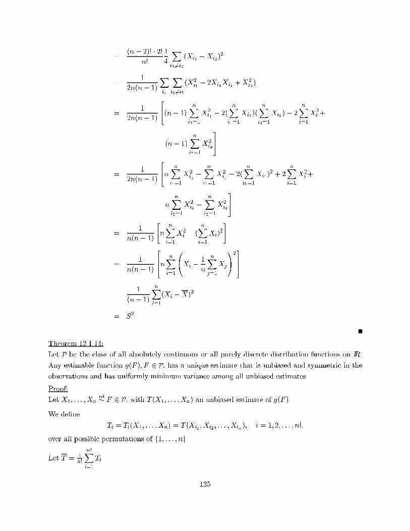
=(n� 2)! � 2!
n!
1
4
Xi1 6=i2
(Xi1 �Xi2)2
=1
2n(n� 1)
Xi1
Xi2 6=i1
(X2i1� 2Xi1Xi2 +X2
i2)
=1
2n(n� 1)
24(n� 1)nX
i1=1
X2i1� 2(
nXi1=1
Xi1)(nX
i2=1
Xi2) + 2nXi=1
X2i +
(n� 1)nX
i2=1
X2i2
35
=1
2n(n� 1)
24n nXi1=1
X2i1�
nXi1=1
X2i1� 2(
nXi1=1
Xi1)2 + 2
nXi=1
X2i +
n
nXi2=1
X2i2�
nXi2=1
X2i2
35=
1
n(n� 1)
"n
nXi=1
X2i � (
nXi=1
Xi)2
#
=1
n(n� 1)
264n nXi=1
0@Xi �1
n
nXj=1
Xj
1A2375
=1
(n� 1)
nXi=1
(Xi �X)2
= S2
Theorem 12.1.14:
Let P be the class of all absolutely continuous or all purely discrete distribution functions on IR.
Any estimable function g(F ); F 2 P, has a unique estimate that is unbiased and symmetric in the
observations and has uniformly minimum variance among all unbiased estimates.
Proof:
Let X1; : : : ; Xn
iid� F 2 P; with T (X1; : : : ; Xn) an unbiased estimate of g(F ).
We de�ne
Ti = Ti(X1; : : : ;Xn) = T (Xi1 ;Xi2 ; : : : ;Xin); i = 1; 2; : : : ; n!;
over all possible permutations of f1; : : : ; ng.
Let T = 1n!
n!Xi=1
Ti.
125
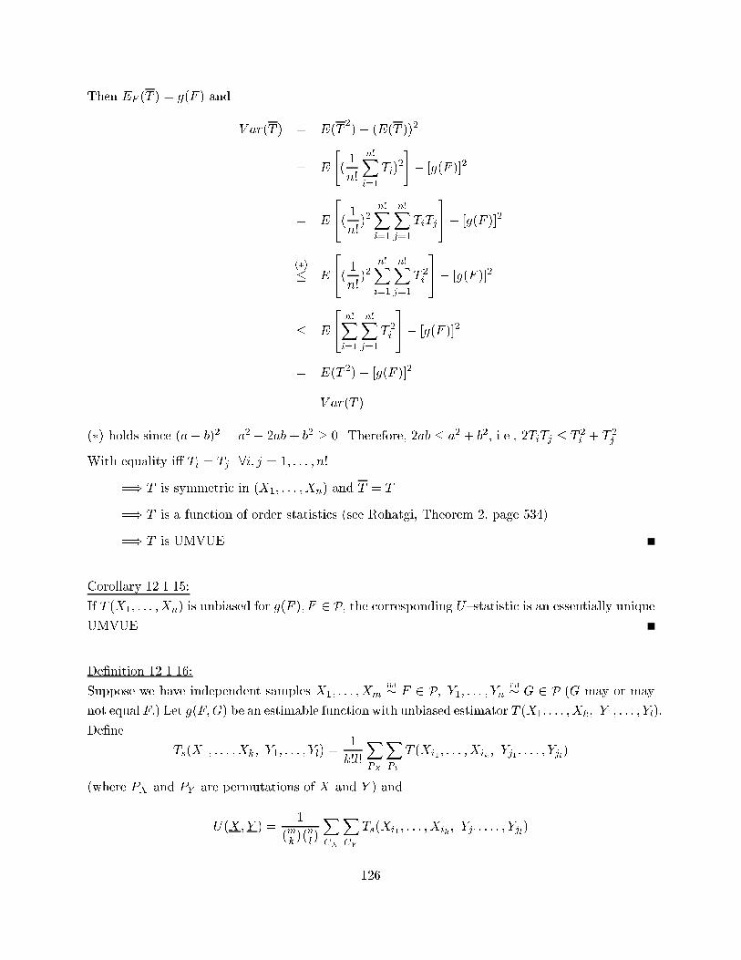
Then EF (T ) = g(F ) and
V ar(T ) = E(T2)� (E(T ))2
= E
"(1
n!
n!Xi=1
Ti)2
#� [g(F )]2
= E
24( 1n!)2
n!Xi=1
n!Xj=1
TiTj
35� [g(F )]2
(�)� E
24( 1n!)2
n!Xi=1
n!Xj=1
T 2i
35� [g(F )]2
� E
24 n!Xi=1
n!Xj=1
T 2i
35� [g(F )]2
= E(T 2)� [g(F )]2
= V ar(T )
(�) holds since (a� b)2 = a2 � 2ab+ b2 � 0. Therefore, 2ab � a2 + b2, i.e., 2TiTj � T 2i+ T 2
j.
With equality i� Ti = Tj 8i; j = 1; : : : ; n!
=) T is symmetric in (X1; : : : ;Xn) and T = T
=) T is a function of order statistics (see Rohatgi, Theorem 2, page 534)
=) T is UMVUE
Corollary 12.1.15:
If T (X1; : : : ;Xn) is unbiased for g(F ); F 2 P, the corresponding U{statistic is an essentially uniqueUMVUE.
De�nition 12.1.16:
Suppose we have independent samples X1; : : : ;Xm
iid� F 2 P; Y1; : : : ; Yniid� G 2 P (G may or may
not equal F:) Let g(F;G) be an estimable function with unbiased estimator T (X1; : : : ;Xk; Y1; : : : ; Yl):
De�ne
Ts(X1; : : : ;Xk; Y1; : : : ; Yl) =1
k!l!
XPX
XPY
T (Xi1 ; : : : ;Xik; Yj1 ; : : : ; Yjl)
(where PX and PY are permutations of X and Y ) and
U(X;Y ) =1�
m
k
��n
l
� XCX
XCY
Ts(Xi1 ; : : : ; Xik; Yj1 ; : : : ; Yjl)
126
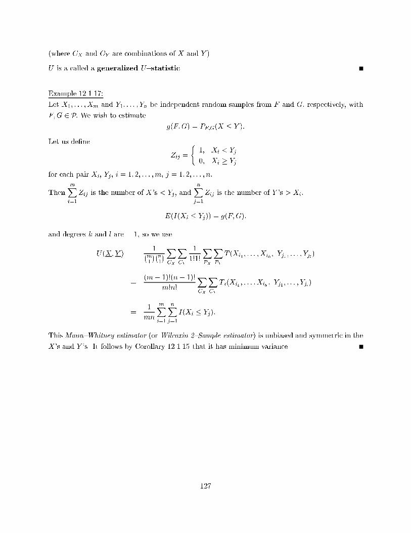
(where CX and CY are combinations of X and Y ).
U is a called a generalized U{statistic.
Example 12.1.17:
Let X1; : : : ;Xm and Y1; : : : ; Yn be independent random samples from F and G, respectively, with
F;G 2 P: We wish to estimate
g(F;G) = PF;G(X � Y ):
Let us de�ne
Zij =
(1; Xi < Yj
0; Xi � Yj
for each pair Xi; Yj; i = 1; 2; : : : ;m; j = 1; 2; : : : ; n:
ThenmXi=1
Zij is the number of X's < Yj; andnXj=1
Zij is the number of Y 's > Xi:
E(I(Xi � Yj)) = g(F;G);
and degrees k and l are = 1, so we use
U(X;Y ) =1�
m
1
��n
1
� XCX
XCY
1
1!1!
XPX
XPY
T (Xi1 ; : : : ; Xik; Yj1 ; : : : ; Yjl)
=(m� 1)!(n� 1)!
m!n!
XCX
XCY
Ts(Xi1 ; : : : ;Xik; Yj1 ; : : : ; Yjl)
=1
mn
mXi=1
nXj=1
I(Xi � Yj):
This Mann{Whitney estimator (or Wilcoxin 2{Sample estimator) is unbiased and symmetric in the
X's and Y 's. It follows by Corollary 12.1.15 that it has minimum variance.
127
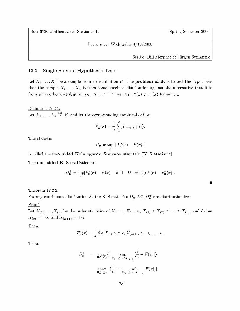
Stat 6720 Mathematical Statistics II Spring Semester 2000
Lecture 38: Wednesday 4/19/2000
Scribe: Bill Morphet & J�urgen Symanzik
12.2 Single-Sample Hypothesis Tests
Let X1; : : : ;Xn be a sample from a distribution F . The problem of �t is to test the hypothesis
that the sample X1; : : : ;Xn is from some speci�ed distribution against the alternative that it is
from some other distribution, i.e., H0 : F = F0 vs. H1 : F (x) 6= F0(x) for some x.
De�nition 12.2.1:
Let X1; : : : ; Xn
iid� F , and let the corresponding empirical cdf be
F �n(x) =1
n
nXi=1
I(�1;x](Xi):
The statistic
Dn = supx
j F �n(x)� F (x) j
is called the two{sided Kolmogorov{Smirnov statistic (K{S statistic).
The one{sided K{S statistics are
D+n = sup
x
[F �n(x)� F (x)] and D�n = sup
x
[F (x) � F �n(x)]:
Theorem 12.2.2:
For any continuous distribution F , the K{S statistics Dn;D�n ;D
+n are distribution free.
Proof:
Let X(1); : : : ;X(n) be the order statistics of X1; : : : ; Xn, i.e., X(1) � X(2) � : : : � X(n), and de�ne
X(0) = �1 and X(n+1) = +1.
Then,
F �n(x) =i
nfor X(i) � x < X(i+1); i = 0; : : : ; n:
Then,
D+n = max
0�i�nf sup
X(i)�x<X(i+1)
[i
n� F (x)]g
= max0�i�n
f in� [ inf
X(i)�x<X(i+1)
F (x)]g
128
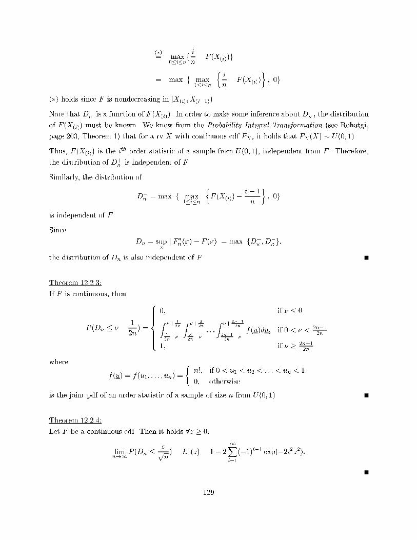
(�)= max
0�i�nf in� F (X(i))g
= max f max1�i�n
�i
n� F (X(i))
�; 0g
(�) holds since F is nondecreasing in [X(i);X(i+1)).
Note that D+n is a function of F (X(i)). In order to make some inference about D
+n , the distribution
of F (X(i)) must be known. We know from the Probability Integral Transformation (see Rohatgi,
page 203, Theorem 1) that for a rv X with continuous cdf FX , it holds that FX(X) � U(0; 1).
Thus, F (X(i)) is the ith order statistic of a sample from U(0; 1), independent from F . Therefore,
the distribution of D+n is independent of F .
Similarly, the distribution of
D�n = max f max
1�i�n
�F (X(i))�
i� 1
n
�; 0g
is independent of F .
Since
Dn = supx
j F �n(x)� F (x) j= max fD+n ; D
�n g;
the distribution of Dn is also independent of F .
Theorem 12.2.3:
If F is continuous, then
P (Dn � � +1
2n) =
8>>>>><>>>>>:
0; if � � 0Z�+ 1
2n
12n��
Z�+ 3
2n
32n��
: : :
Z�+ 2n�1
2n
2n�12n
��f(u)du; if 0 < � < 2n�1
2n
1; if � � 2n�12n
where
f(u) = f(u1; : : : ; un) =
(n!; if 0 < u1 < u2 < : : : < un < 1
0; otherwise
is the joint pdf of an order statistic of a sample of size n from U(0; 1).
Theorem 12.2.4:
Let F be a continuous cdf. Then it holds 8z � 0:
limn!1
P (Dn �zpn) = L1(z) = 1� 2
1Xi=1
(�1)i�1 exp(�2i2z2):
129
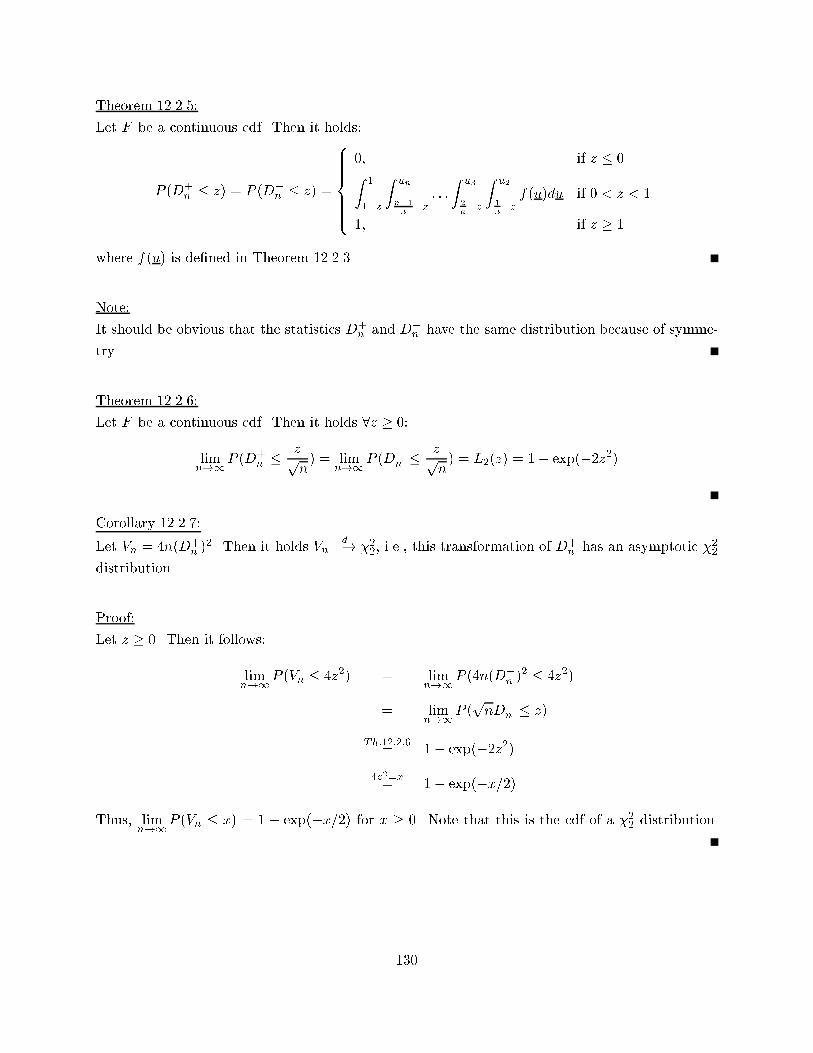
Theorem 12.2.5:
Let F be a continuous cdf. Then it holds:
P (D+n � z) = P (D�
n � z) =
8>>>>><>>>>>:0; if z � 0Z 1
1�z
Zun
n�1n�z: : :
Zu3
2n�z
Zu2
1n�zf(u)du if 0 < z < 1
1; if z � 1
where f(u) is de�ned in Theorem 12.2.3.
Note:
It should be obvious that the statistics D+n and D�
n have the same distribution because of symme-
try.
Theorem 12.2.6:
Let F be a continuous cdf. Then it holds 8z � 0:
limn!1
P (D+n �
zpn) = lim
n!1P (D�
n �zpn) = L2(z) = 1� exp(�2z2)
Corollary 12.2.7:
Let Vn = 4n(D+n )
2. Then it holds Vnd�! �22, i.e., this transformation of D+
n has an asymptotic �22
distribution.
Proof:
Let z � 0. Then it follows:
limn!1
P (Vn � 4z2) = limn!1
P (4n(D+n )
2 � 4z2)
= limn!1
P (pnD+
n � z)
Th:12:2:6= 1� exp(�2z2)
4z2=x= 1� exp(�x=2)
Thus, limn!1
P (Vn � x) = 1 � exp(�x=2) for x � 0. Note that this is the cdf of a �22 distribution.
130
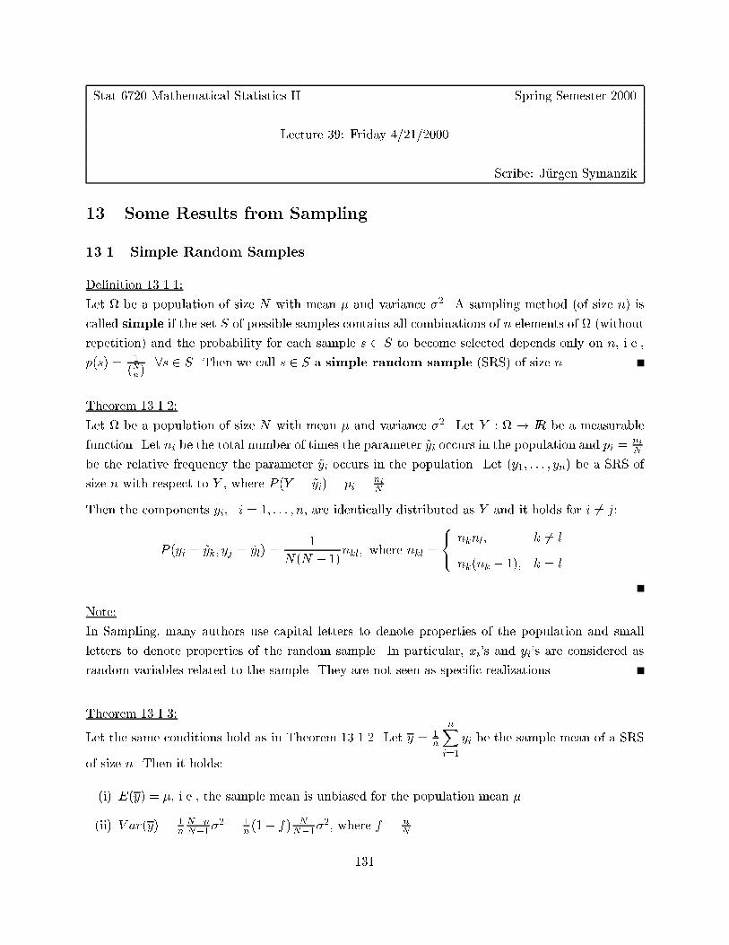
Stat 6720 Mathematical Statistics II Spring Semester 2000
Lecture 39: Friday 4/21/2000
Scribe: J�urgen Symanzik
13 Some Results from Sampling
13.1 Simple Random Samples
De�nition 13.1.1:
Let be a population of size N with mean � and variance �2. A sampling method (of size n) is
called simple if the set S of possible samples contains all combinations of n elements of (without
repetition) and the probability for each sample s 2 S to become selected depends only on n, i.e.,
p(s) = 1
(Nn)8s 2 S. Then we call s 2 S a simple random sample (SRS) of size n.
Theorem 13.1.2:
Let be a population of size N with mean � and variance �2. Let Y : ! IR be a measurable
function. Let ni be the total number of times the parameter ~yi occurs in the population and pi =ni
N
be the relative frequency the parameter ~yi occurs in the population. Let (y1; : : : ; yn) be a SRS of
size n with respect to Y , where P (Y = ~yi) = pi =ni
N.
Then the components yi; i = 1; : : : ; n, are identically distributed as Y and it holds for i 6= j:
P (yi = ~yk; yj = ~yl) =1
N(N � 1)nkl; where nkl =
8<: nknl; k 6= l
nk(nk � 1); k = l
Note:
In Sampling, many authors use capital letters to denote properties of the population and small
letters to denote properties of the random sample. In particular, xi's and yi's are considered as
random variables related to the sample. They are not seen as speci�c realizations.
Theorem 13.1.3:
Let the same conditions hold as in Theorem 13.1.2. Let y = 1n
nXi=1
yi be the sample mean of a SRS
of size n. Then it holds:
(i) E(y) = �, i.e., the sample mean is unbiased for the population mean �.
(ii) V ar(y) = 1n
N�nN�1�
2 = 1n(1� f) N
N�1�2, where f = n
N.
131
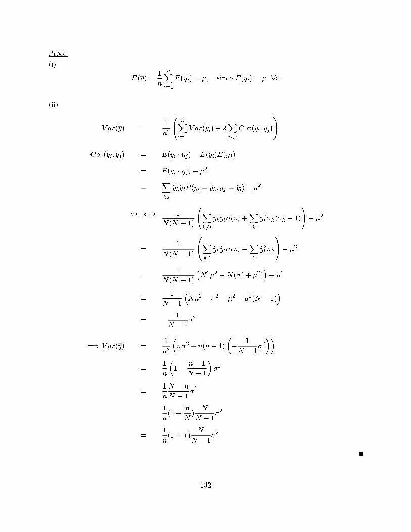
Proof:
(i)
E(y) =1
n
nXi=1
E(yi) = �; since E(yi) = � 8i:
(ii)
V ar(y) =1
n2
0@ nXi=1
V ar(yi) + 2Xi<j
Cov(yi; yj)
1ACov(yi; yj) = E(yi � yj)�E(yi)E(yj)
= E(yi � yj)� �2
=Xk;l
~yk~ylP (yi = ~yk; yj = ~yl)� �2
Th:13:1:2=
1
N(N � 1)
0@Xk 6=l
~yk~ylnknl +Xk
~y2knk(nk � 1)
1A� �2
=1
N(N � 1)
0@Xk;l
~yk~ylnknl �Xk
~y2knk
1A� �2
=1
N(N � 1)
�N2�2 �N(�2 + �2)
�� �2
=1
N � 1
�N�2 � �2 � �2 � �2(N � 1)
�= � 1
N � 1�2
=) V ar(y) =1
n2
�n�2 + n(n� 1)
�� 1
N � 1�2��
=1
n
�1� n� 1
N � 1
��2
=1
n
N � n
N � 1�2
=1
n(1� n
N)
N
N � 1�2
=1
n(1� f)
N
N � 1�2
132
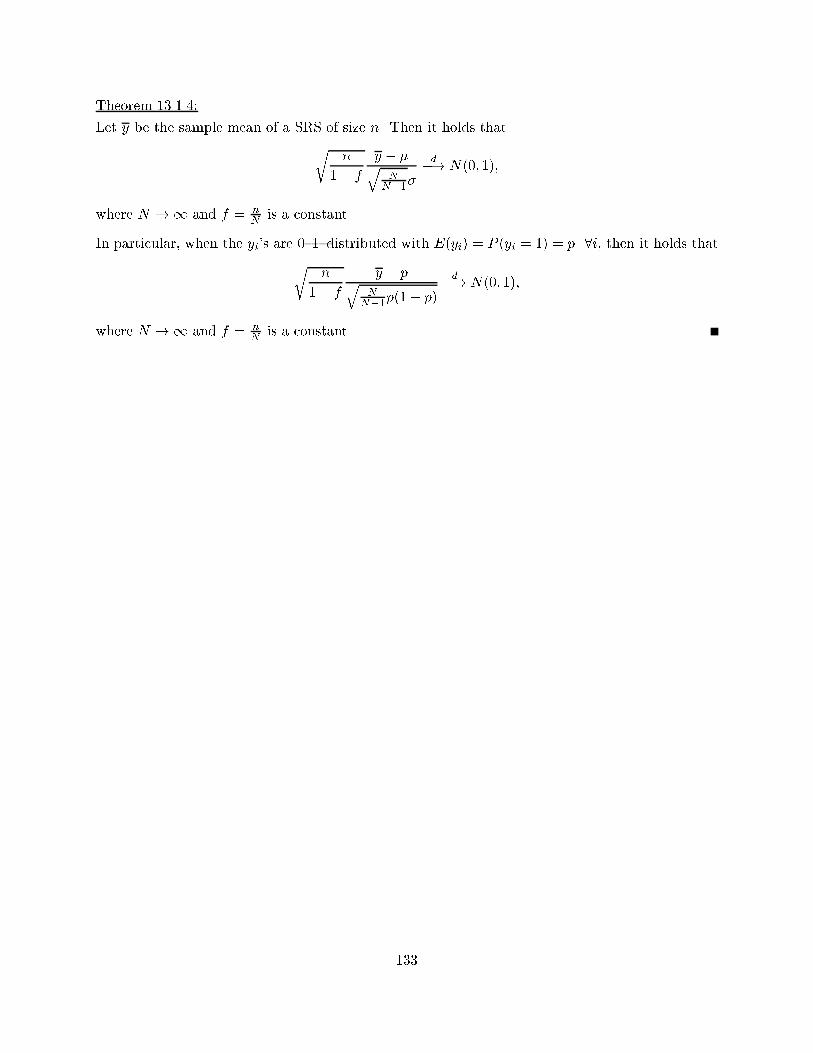
Theorem 13.1.4:
Let y be the sample mean of a SRS of size n. Then it holds thatrn
1� f
y � �qN
N�1�
d�! N(0; 1);
where N !1 and f = n
Nis a constant.
In particular, when the yi's are 0{1{distributed with E(yi) = P (yi = 1) = p 8i, then it holds thatrn
1� f
y � pqN
N�1p(1� p)
d�! N(0; 1);
where N !1 and f = n
Nis a constant.
133
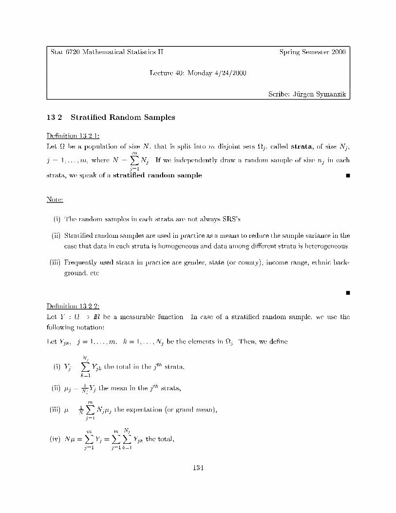
Stat 6720 Mathematical Statistics II Spring Semester 2000
Lecture 40: Monday 4/24/2000
Scribe: J�urgen Symanzik
13.2 Strati�ed Random Samples
De�nition 13.2.1:
Let be a population of size N , that is split into m disjoint sets j, called strata, of size Nj ,
j = 1; : : : ;m, where N =mXj=1
Nj. If we independently draw a random sample of size nj in each
strata, we speak of a strati�ed random sample.
Note:
(i) The random samples in each strata are not always SRS's.
(ii) Strati�ed random samples are used in practice as a means to reduce the sample variance in the
case that data in each strata is homogeneous and data among di�erent strata is heterogeneous.
(iii) Frequently used strata in practice are gender, state (or county), income range, ethnic back-
ground, etc.
De�nition 13.2.2:
Let Y : ! IR be a measurable function. In case of a strati�ed random sample, we use the
following notation:
Let Yjk; j = 1; : : : ;m; k = 1; : : : ; Nj be the elements in j. Then, we de�ne
(i) Yj =
NjXk=1
Yjk the total in the jth strata,
(ii) �j =1NjYj the mean in the jth strata,
(iii) � = 1N
mXj=1
Nj�j the expectation (or grand mean),
(iv) N� =mXj=1
Yj =mXj=1
NjXk=1
Yjk the total,
134
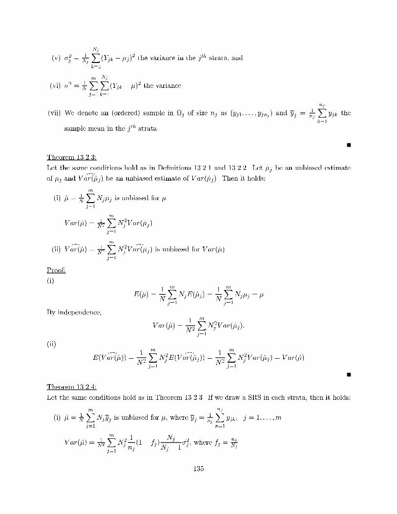
(v) �2j= 1
Nj
NjXk=1
(Yjk � �j)2 the variance in the jth strata, and
(vi) �2 = 1N
mXj=1
NjXk=1
(Yjk � �)2 the variance.
(vii) We denote an (ordered) sample in j of size nj as (yj1; : : : ; yjnj ) and yj = 1nj
njXk=1
yjk the
sample mean in the jth strata.
Theorem 13.2.3:
Let the same conditions hold as in De�nitions 13.2.1 and 13.2.2. Let �̂j be an unbiased estimate
of �j anddV ar(�̂j) be an unbiased estimate of V ar(�̂j). Then it holds:
(i) �̂ = 1N
mXj=1
Nj�̂j is unbiased for �.
V ar(�̂) = 1N2
mXj=1
N2j V ar(�̂j).
(ii) dV ar(�̂) = 1N2
mXj=1
N2j
dV ar(�̂j) is unbiased for V ar(�̂).
Proof:
(i)
E(�̂) =1
N
mXj=1
NjE(�̂j) =1
N
mXj=1
Nj�j = �
By independence,
V ar(�̂) =1
N2
mXj=1
N2j V ar(�̂j):
(ii)
E( dV ar(�̂)) = 1
N2
mXj=1
N2j E(
dV ar(�̂j)) =1
N2
mXj=1
N2j V ar(�̂j) = V ar(�̂)
Theorem 13.2.4:
Let the same conditions hold as in Theorem 13.2.3. If we draw a SRS in each strata, then it holds:
(i) �̂ = 1N
mXj=1
Njyj is unbiased for �, where yj =1nj
njXk=1
yjk; j = 1; : : : ;m.
V ar(�̂) = 1N2
mXj=1
N2j
1
nj(1� fj)
Nj
Nj � 1�2j , where fj =
nj
Nj.
135
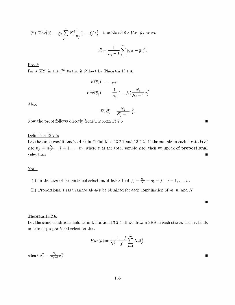
(ii) dV ar(�̂) = 1N2
mXj=1
N2j
1
nj(1� fj)s
2j is unbiased for V ar(�̂), where
s2j =1
nj � 1
njXk=1
(yjk � yj)2:
Proof:
For a SRS in the jth strata, it follows by Theorem 13.1.3:
E(yj) = �j
V ar(yj) =1
nj(1� fj)
Nj
Nj � 1�2j
Also,
E(s2j ) =Nj
Nj � 1�2j :
Now the proof follows directly from Theorem 13.2.3.
De�nition 13.2.5:
Let the same conditions hold as in De�nitions 13.2.1 and 13.2.2. If the sample in each strata is of
size nj = nNj
N; j = 1; : : : ;m, where n is the total sample size, then we speak of proportional
selection.
Note:
(i) In the case of proportional selection, it holds that fj =nj
Nj= n
N= f; j = 1; : : : ;m.
(ii) Proportional strata cannot always be obtained for each combination of m, n, and N .
Theorem 13.2.6:
Let the same conditions hold as in De�nition 13.2.5. If we draw a SRS in each strata, then it holds
in case of proportional selection that
V ar(�̂) =1
N2
1� f
f
mXj=1
Nj~�2j ;
where ~�2j=
Nj
Nj�1�2j.
136
Theorem 13.2.7:
If we draw (1) a strati�ed random sample that consists of SRS's of sizes nj under proportional
selection and (2) a SRS of size n =mXj=1
nj from the same population, then it holds that
V ar(y)� V ar(�̂) =1
n
N � n
N(N � 1)
0@ mXj=1
Nj(�j � �)2 � 1
N
mXj=1
(N �Nj)~�2j
1A :
137
Stat 6720 Mathematical Statistics II Spring Semester 2000
Lecture 41: Wednesday 4/26/2000
Scribe: J�urgen Symanzik
14 Some Results from Sequential Statistical Inference
14.1 Fundamentals of Sequential Sampling
Example 14.1.1:
A particular machine produces a large number of items every day. Each item can be either \de-
fective" or \non{defective". The unknown proportion of defective items in the production of a
particular day is p.
Let (X1; : : : ;Xm) be a sample from the daily production where xi = 1 when the item is defective
and xi = 0 when the item is non{defective. Obviously, Sm =mXi=1
Xi � Bin(m; p) denotes the
total number of defective items in the sample (assuming that m is small compared to the daily
production).
We might be interested to test H0 : p � p0 vs. H1 : p > p0 at a given signi�cance level � and use
this decision to trash the entire daily production and have the machine �xed if indeed p > p0. A
suitable test could be
�1(x1; : : : ; xm) =
8<: 1; if sm > c
0; if sm � c
where c is chosen such that �1 is a level{� test.
However, wouldn't it be more bene�cial if we sequentially sample the items (e.g., take item # 57,
623, 1005, 1286, 2663, etc.) and stop the machine as soon as it becomes obvious that it produces
too many bad items. (Alternatively, we could also �nish the time consuming and expensive process
to determine whether an item is defective or non{defective if it is impossible to surpass a certain
proportion of defectives.) For example, if for some j < m it already holds that sj > c, then we
could stop (and immediately call maintenance) and reject H0 after only j observations.
More formally, let us de�ne T = minfj j Sj > cg and T 0 = minfT;mg. We can now consider
a decision rule that stops with the sampling process at random time T 0 and rejects H0 if T � m.
Thus, if we consider R0 = f(x1; : : : ; xm) j t � mg and R1 = f(x1; : : : ; xm) j sm > cg as criticalregions of two tests �0 and �1, then these two tests are equivalent.
138
De�nition 14.1.2:
Let � be the parameter space and A the set of actions the statistician can take. We assume that the
rv's X1;X2; : : : are observed sequentially and iid with common pdf (or pmf) f�(x). A sequential
decision procedure is de�ned as follows:
(i) A stopping rule speci�es whether an element of A should be chosen without taking any
further observation. If at least one observation is taken, this rule speci�es for every set of
observed values (x1; x2; : : : ; xn), n � 1, whether to stop sampling and choose an action in A
or to take another observation xn+1.
(ii) A decision rule speci�es the decision to be taken. If no observation has been taken, then we
take action d0 2 A. If n � 1 observation have been taken, then we take action dn(x1; : : : ; xn) 2A, where dn(x1; : : : ; xn) speci�es the action that has to be taken for the set (x1; : : : ; xn) of
observed values. Once an action has been taken, the sampling process is stopped.
Note:
In the remainder of this chapter, we assume that the statistician takes at least one observation.
De�nition 14.1.3:
Let Rn � IRn; n = 1; 2; : : :, be a sequence of Borel{measurable sets such that the sampling process is
stopped after observing X1 = x1; X2 = x2; : : : ; Xn = xn if (x1; : : : ; xn) 2 Rn. If (x1; : : : ; xn) =2 Rn,
then another observation xn+1 is taken. The sets Rn; n = 1; 2; : : : are called stopping regions.
De�nition 14.1.4:
With every sequential stopping rule we associate a stopping random variable N which takes on
the values 1; 2; 3; : : :. Thus, N is rv that indicates the total number of observations taken before
the sampling is stopped.
Note:
We use the (sloppy) notation fN = ng to denote the event that sampling is stopped after observingexactly n values x1; : : : ; xn (i.e., sampling is not stopped before taking n samples). Then the
following equalities hold:
fN = 1g = R1
fN = ng = f(x1; : : : ; xn) 2 IRn j sampling is stopped after n observations but not beforeg
= (R1 [R2 [ : : : [Rn�1)c \Rn
= Rc
1 \Rc
2 \ : : : \Rc
n�1 \Rn
139
fN � ng =n[
k=1
fN = kg
Here we will only consider closed sequential sampling procedures, i.e., procedures where sampling
eventually stops with probability 1, i.e.,
P (N <1) = 1;
P (N =1) = 1� P (N <1) = 0:
140
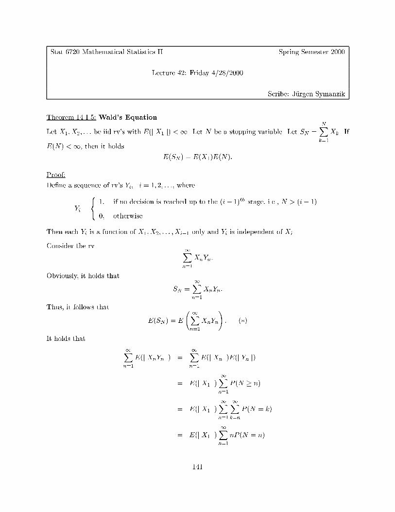
Stat 6720 Mathematical Statistics II Spring Semester 2000
Lecture 42: Friday 4/28/2000
Scribe: J�urgen Symanzik
Theorem 14.1.5: Wald's Equation
Let X1; X2; : : : be iid rv's with E(j X1 j) <1. Let N be a stopping variable. Let SN =NXk=1
Xk. If
E(N) <1, then it holds
E(SN ) = E(X1)E(N):
Proof:
De�ne a sequence of rv's Yi; i = 1; 2; : : :, where
Yi =
8<: 1; if no decision is reached up to the (i� 1)th stage, i.e., N > (i� 1)
0; otherwise
Then each Yi is a function of X1;X2; : : : ;Xi�1 only and Yi is independent of Xi.
Consider the rv 1Xn=1
XnYn:
Obviously, it holds that
SN =1Xn=1
XnYn:
Thus, it follows that
E(SN ) = E
1Xn=1
XnYn
!: (�)
It holds that
1Xn=1
E(j XnYn j) =1Xn=1
E(j Xn j)E(j Yn j)
= E(j X1 j)1Xn=1
P (N � n)
= E(j X1 j)1Xn=1
1Xk=n
P (N = k)
= E(j X1 j)1Xn=1
nP (N = n)
141

= E(j X1 j)E(N)
< 1
We may therefore interchange the expectation and summation signs in (�) and get
E(SN ) = E
1Xn=1
XnYn
!
=1Xn=1
E(XnYn)
=1Xn=1
E(Xn)E(Yn)
= E(X1)1Xn=1
P (N � n)
= E(X1)E(N)
which completes the proof.
142
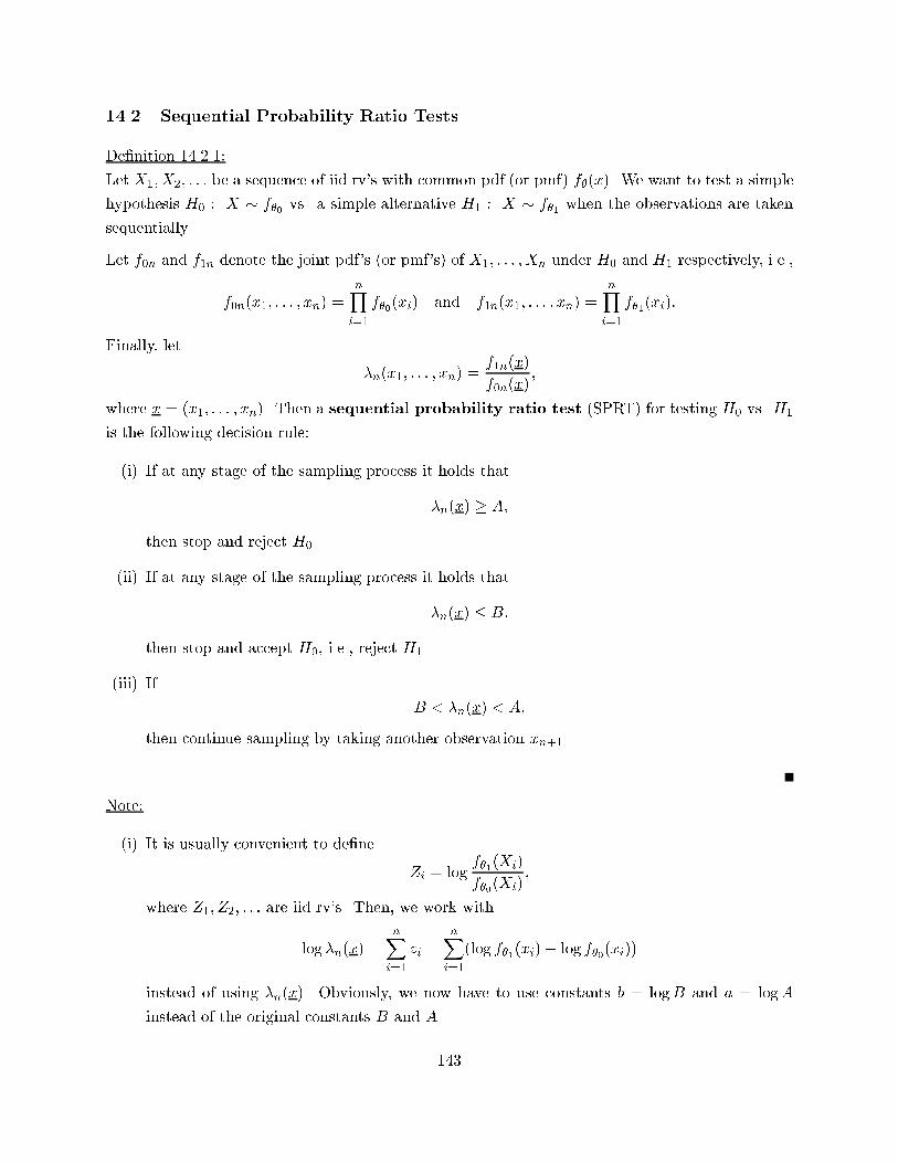
14.2 Sequential Probability Ratio Tests
De�nition 14.2.1:
Let X1;X2; : : : be a sequence of iid rv's with common pdf (or pmf) f�(x). We want to test a simple
hypothesis H0 : X � f�0 vs. a simple alternative H1 : X � f�1 when the observations are taken
sequentially.
Let f0n and f1n denote the joint pdf's (or pmf's) of X1; : : : ; Xn under H0 and H1 respectively, i.e.,
f0n(x1; : : : ; xn) =nYi=1
f�0(xi) and f1n(x1; : : : ; xn) =nYi=1
f�1(xi):
Finally, let
�n(x1; : : : ; xn) =f1n(x)
f0n(x);
where x = (x1; : : : ; xn). Then a sequential probability ratio test (SPRT) for testing H0 vs. H1
is the following decision rule:
(i) If at any stage of the sampling process it holds that
�n(x) � A;
then stop and reject H0.
(ii) If at any stage of the sampling process it holds that
�n(x) � B;
then stop and accept H0, i.e., reject H1.
(iii) If
B < �n(x) < A;
then continue sampling by taking another observation xn+1.
Note:
(i) It is usually convenient to de�ne
Zi = logf�1(Xi)
f�0(Xi);
where Z1; Z2; : : : are iid rv's. Then, we work with
log �n(x) =nXi=1
zi =nXi=1
(log f�1(xi)� log f�0(xi))
instead of using �n(x). Obviously, we now have to use constants b = logB and a = logA
instead of the original constants B and A.
143
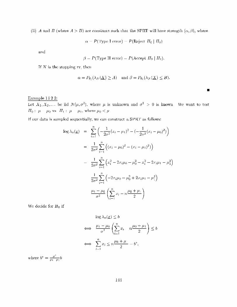
(ii) A and B (where A > B) are constants such that the SPRT will have strength (�; �), where
� = P (Type I error) = P (Reject H0 j H0)
and
� = P (Type II error) = P (Accept H0 j H1):
If N is the stopping rv, then
� = P�0(�N (X) � A) and � = P�1(�N (X) � B):
Example 14.2.2:
Let X1;X2; : : : be iid N(�; �2), where � is unknown and �2 > 0 is known. We want to test
H0 : � = �0 vs. H1 : � = �1, where �0 < �1.
If our data is sampled sequentially, we can constract a SPRT as follows:
log �n(x) =nXi=1
�� 1
2�2(xi � �1)
2 � (� 1
2�2(xi � �0)
2)
�
=1
2�2
nXi=1
�(xi � �0)
2 � (xi � �1)2)�
=1
2�2
nXi=1
�x2i � 2xi�0 + �20 � x2i + 2xi�1 � �21
�
=1
2�2
nXi=1
��2xi�0 + �20 + 2xi�1 � �21
�
=�1 � �0
�2
nXi=1
xi � n�0 + �1
2
!
We decide for H0 if
log �n(x) � b
() �1 � �0
�2
nXi=1
xi � n�0 + �1
2
!� b
()nXi=1
xi � n�0 + �1
2+ b�;
where b� = �2
�1��0 b.
144
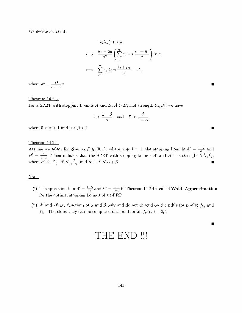
We decide for H1 if
log �n(x) � a
() �1 � �0
�2
nXi=1
xi � n�0 + �1
2
!� a
()nXi=1
xi � n�0 + �1
2+ a�;
where a� = �2
�1��0a.
Theorem 14.2.3:
For a SPRT with stopping bounds A and B, A > B, and strength (�; �), we have
A � 1� �
�and B � �
1� �;
where 0 < � < 1 and 0 < � < 1.
Theorem 14.2.4:
Assume we select for given �; � 2 (0; 1), where � + � � 1, the stopping bounds A0 = 1���
and
B0 = �
1�� . Then it holds that the SPRT with stopping bounds A0 and B0 has strength (�0; �0),
where �0 � �
1�� , �0 � �
1�� , and �0 + �0 � �+ �.
Note:
(i) The approximationA0 = 1���
andB0 = �
1�� in Theorem 14.2.4 is calledWald{Approximation
for the optimal stopping bounds of a SPRT.
(ii) A0 and B0 are functions of � and � only and do not depend on the pdf's (or pmf's) f�0 and
f�1 . Therefore, they can be computed once and for all f�i 's, i = 0; 1.
THE END !!!
145

Index
�{similar, 77
0{1 Loss, 99
A Posteriori Distribution, 56
A Priori Distribution, 56
Action, 53
Alternative Hypothesis, 60
Asymptotically (Most) E�cient, 43
Bayes Estimate, 57
Bayes Risk, 56
Bayes Rule, 57
Bayesian Con�dence Set, 120
Bias, 27
Central Limit Theorem, Lindeberg, 5
Central Limit Theorem, Lindeberg{L�evy, 2
Chapman, Robbins, Kiefer Inequality, 41
CI, 106
Closed, 140
Complete, 23, 121
Complete in Relation to P, 121
Composite, 60
Con�dence Bound, Lower, 106
Con�dence Bound, Upper, 106
Con�dence Coe�cient, 106
Con�dence Interval, 106
Con�dence Level, 105
Con�dence Sets, 105
Consistent in the rthMean, 17
Consistent, Mean{Squared{Error, 28
Consistent, Strongly, 17
Consistent, Weakly, 17
Continuity Theorem, 1
Contradiction, Proof by, 30
Cram�er{Rao Lower Bound, 37
Credible Set, 120
Critical Region, 61
CRK Inequality, 41
CRLB, 37
Decision Function, 53
Decision Rule, 139
Degree, 122
Distribution, Population, 8
Distribution{Free, 121
Domain of Attraction, 4
E�ciency, 43
E�cient, Asymptotically (Most), 43
E�cient, More, 43
E�cient, Most, 43
Empirical Cumulative Distribution Function, 8
Error, Type I, 61
Error, Type II, 61
Estimable, 122
Estimable Function, 27
Estimate, Bayes, 57
Estimate, Maximum Likelihood, 46
Estimate, Method of Moments, 45
Estimate, Minimax, 54
Estimate, Point, 16
Estimator, 16
Estimator, Mann{Whitney, 127
Estimator, Wilcoxin 2{Sample, 127
Exponential Family, One{Parameter, 25
F{Test, 97
Factorization Criterion, 21
Family of CDF's, 16
Family of Con�dence Sets, 105
Family of PDF's, 16
Family of PMF's, 16
Family of Random Sets, 105
Formal Invariance, 80
Generalized U{Statistic, 127
Glivenko{Cantelli Theorem, 9
Hypothesis, Alternative, 60
Hypothesis, Null, 60
Independence of X and S2, 13
Induced Function, 18
Interval, Random, 105
Invariance, Measurement, 80
Invariant, 18, 80
Invariant Test, 81
Invariant, Location, 18
Invariant, Maximal, 83
Invariant, Permutation, 18
Invariant, Scale, 18
K{S Statistic, 128
Kernel, 122
Kernel, Symmetric, 122
Kolmogorov{Smirnov Statistic, 128
Landau Symbols O and o, 3
Lehmann{Sche��ee, 35
Level of Signi�cance, 62
Level{�{Test, 62
Likelihood Function, 46
Likelihood Ratio Test, 86
Likelihood Ratio Test Statistic, 86
Lindeberg Central Limit Theorem, 5
146

Lindeberg Condition, 5
Lindeberg{L�evy Central Limit Theorem, 2
LMVUE, 29
Locally Minumum Variance Unbiased Estimate, 29
Location Invariant, 18
Logic, 30
Loss Function, 53
Lower Con�dence Bound, 106
LRT, 86
Mann{Whitney Estimator, 127
Maximal Invariant, 83
Maximum Likelihood Estimate, 46
Mean Square Error, 28
Mean{Squared{Error Consistent, 28
Measurement Invariance, 80
Method of Moments Estimate, 45
Minimax Estimate, 54
Minimax Principle, 54
MLE, 46
MLR, 68
Monotone Likelihood Ratio, 68
More E�cient, 43
Most E�cient, 43
Most Powerful Test, 62
MP, 62
MSE{Consistent, 28
Neyman{Pearson Lemma, 65
Nonparametric, 121
Nonrandomized Test, 62
Normal Variance Tests, 91
NP Lemma, 65
Null Hypothesis, 60
One Sample t{Test, 95
One{Tailed t-Test, 95
Paired t-Test, 96
Parameter Space, 16
Parametric Hypothesis, 60
Permutation Invariant, 18
Pivot, 109
Point Estimate, 16
Point Estimation, 16
Population Distribution, 8
Power, 62
Power Function, 62
Probability Integral Transformation, 129
Probability Ratio Test, Sequential, 143
Problem of Fit, 128
Proof by Contradiction, 30
Proportional Selection, 136
Random Interval, 105
Random Sample, 8
Random Sets, 105
Random Variable, Stopping, 139
Randomized Test, 62
Rao{Blackwell, 34
Rao{Blackwellization, 35
Realization, 8
Regularity Conditions, 38
Risk Function, 53
Risk, Bayes, 56
Sample, 8
Sample Central Moment of Order k, 9
Sample Mean, 8
Sample Moment of Order k, 9
Sample Statistic, 8
Sample Variance, 8
Scale Invariant, 18
Selection, Proportional, 136
Sequential Decision Procedure, 139
Sequential Probability Ratio Test, 143
Signi�cance Level, 62
Similar, 77
Similar, �, 77
Simple, 60, 131
Simple Random Sample, 131
Size, 62
SPRT, 143
SRS, 131
Stable, 4
Statistic, 8
Statistic, Kolmogorov{Smirnov, 128
Statistic, Likelihood Ratio Test, 86
Stopping Random Variable, 139
Stopping Regions, 139
Stopping Rule, 139
Strata, 134
Strati�ed Random Sample, 134
Strongly Consistent, 17
Su�cient, 19, 121
Symmetric Kernel, 122
t{Test, 95
Test Function, 62
Test, Invariant, 81
Test, Likelihood Ratio, 86
Test, Most Powerful, 62
Test, Nonrandomized, 62
Test, Randomized, 62
Test, Uniformly Most Powerful, 62
Two{Sample t-Test, 95
Two{Tailed t-Test, 95
Type I Error, 61
Type II Error, 61
147
U{Statistic, 124
U{Statistic, Generalized, 127
UMA, 106
UMAU, 116
UMP, 62
UMP �{similar, 77
UMP Invariant, 83
UMP Unbiased, 72
UMPU, 72
UMVUE, 29
Unbiased, 27, 72, 116
Uniformly Minumum Variance Unbiased Estimate, 29
Uniformly Most Accurate, 106
Uniformly Most Accurate Unbiased, 116
Uniformly Most Powerful Test, 62
Unimodal, 111
Upper Con�dence Bound, 106
Wald's Equation, 141
Wald{Approximation, 145
Weakly Consistent, 17
Wilcoxin 2{Sample Estimator, 127
148