Embed Size (px)
Citation preview

Advanced Quantum Field Theory(Version of September 2016)
Jorge Crispim Romao
Physics Department2016


Contents
1 Free Field Quantization 13
1.1 General formalism . . . . . . . . . . . . . . . . . . . . . . . . . . . . . . . . 13
1.1.1 Canonical quantization for particles . . . . . . . . . . . . . . . . . . 13
1.1.2 Canonical quantization for fields . . . . . . . . . . . . . . . . . . . . 17
1.1.3 Symmetries and conservation laws . . . . . . . . . . . . . . . . . . . 19
1.2 Quantization of scalar fields . . . . . . . . . . . . . . . . . . . . . . . . . . . 23
1.2.1 Real scalar field . . . . . . . . . . . . . . . . . . . . . . . . . . . . . . 23
1.2.2 Microscopic causality . . . . . . . . . . . . . . . . . . . . . . . . . . . 27
1.2.3 Vacuum fluctuations . . . . . . . . . . . . . . . . . . . . . . . . . . . 28
1.2.4 Charged scalar field . . . . . . . . . . . . . . . . . . . . . . . . . . . 28
1.2.5 Time ordered product and the Feynman propagator . . . . . . . . . 30
1.3 Second quantization of the Dirac field . . . . . . . . . . . . . . . . . . . . . 32
1.3.1 Canonical formalism for the Dirac field . . . . . . . . . . . . . . . . 32
1.3.2 Microscopic causality . . . . . . . . . . . . . . . . . . . . . . . . . . . 35
1.3.3 Feynman propagator . . . . . . . . . . . . . . . . . . . . . . . . . . . 36
1.4 Electromagnetic field quantization . . . . . . . . . . . . . . . . . . . . . . . 37
1.4.1 Introduction . . . . . . . . . . . . . . . . . . . . . . . . . . . . . . . 37
1.4.2 Undefined metric formalism . . . . . . . . . . . . . . . . . . . . . . . 39
1.4.3 Feynman propagator . . . . . . . . . . . . . . . . . . . . . . . . . . . 46
1.5 Discrete Symmetries . . . . . . . . . . . . . . . . . . . . . . . . . . . . . . . 47
1.5.1 Parity . . . . . . . . . . . . . . . . . . . . . . . . . . . . . . . . . . . 47
1.5.2 Charge conjugation . . . . . . . . . . . . . . . . . . . . . . . . . . . . 49
1.5.3 Time reversal . . . . . . . . . . . . . . . . . . . . . . . . . . . . . . . 50
1.5.4 The T CP theorem . . . . . . . . . . . . . . . . . . . . . . . . . . . . 51
Problems for Chapter 1 . . . . . . . . . . . . . . . . . . . . . . . . . . . . . . . . 52
2 Physical States. S Matrix. LSZ Reduction. 55
2.1 Physical states . . . . . . . . . . . . . . . . . . . . . . . . . . . . . . . . . . 55
2.2 In states . . . . . . . . . . . . . . . . . . . . . . . . . . . . . . . . . . . . . . 56
3

4 CONTENTS
2.3 Spectral representation for scalar fields . . . . . . . . . . . . . . . . . . . . . 58
2.4 Out states . . . . . . . . . . . . . . . . . . . . . . . . . . . . . . . . . . . . . 60
2.5 S matrix . . . . . . . . . . . . . . . . . . . . . . . . . . . . . . . . . . . . . . 61
2.6 Reduction formula for scalar fields . . . . . . . . . . . . . . . . . . . . . . . 62
2.7 Reduction formula for fermions . . . . . . . . . . . . . . . . . . . . . . . . . 65
2.7.1 States in and out . . . . . . . . . . . . . . . . . . . . . . . . . . . . . 65
2.7.2 Spectral representation fermions . . . . . . . . . . . . . . . . . . . . 66
2.7.3 Reduction formula fermions . . . . . . . . . . . . . . . . . . . . . . . 68
2.8 Reduction formula for photons . . . . . . . . . . . . . . . . . . . . . . . . . 70
2.9 Cross sections . . . . . . . . . . . . . . . . . . . . . . . . . . . . . . . . . . . 72
Problems for Chapter 2 . . . . . . . . . . . . . . . . . . . . . . . . . . . . . . . . 75
3 Covariant Perturbation Theory 77
3.1 U matrix . . . . . . . . . . . . . . . . . . . . . . . . . . . . . . . . . . . . . 77
3.2 Perturbative expansion of Green functions . . . . . . . . . . . . . . . . . . . 80
3.3 Wick’s theorem . . . . . . . . . . . . . . . . . . . . . . . . . . . . . . . . . . 82
3.4 Vacuum–Vacuum amplitudes . . . . . . . . . . . . . . . . . . . . . . . . . . 87
3.5 Feynman rules for λϕ4 . . . . . . . . . . . . . . . . . . . . . . . . . . . . . . 88
3.6 Feynman rules for QED . . . . . . . . . . . . . . . . . . . . . . . . . . . . . 93
3.6.1 Compton scattering . . . . . . . . . . . . . . . . . . . . . . . . . . . 94
3.6.2 Electron–positron elastic scattering (Bhabha scattering) . . . . . . . 98
3.6.3 Fermion Loops . . . . . . . . . . . . . . . . . . . . . . . . . . . . . . 100
3.6.4 Feynman rules for QED . . . . . . . . . . . . . . . . . . . . . . . . . 102
3.7 General formalism for getting the Feynman rules . . . . . . . . . . . . . . . 103
3.7.1 Example: scalar electrodynamics . . . . . . . . . . . . . . . . . . . . 105
Problems for Chapter 3 . . . . . . . . . . . . . . . . . . . . . . . . . . . . . . . . 108
4 Radiative Corrections 111
4.1 QED Renormalization at one-loop . . . . . . . . . . . . . . . . . . . . . . . 111
4.1.1 Vacuum Polarization . . . . . . . . . . . . . . . . . . . . . . . . . . . 112
4.1.2 Self-energy of the electron . . . . . . . . . . . . . . . . . . . . . . . . 121
4.1.3 The Vertex . . . . . . . . . . . . . . . . . . . . . . . . . . . . . . . . 125
4.2 Ward-Takahashi identities in QED . . . . . . . . . . . . . . . . . . . . . . . 130
4.2.1 Transversality of the photon propagator n = 0, p = 1 . . . . . . . . . 131
4.2.2 Identity for the vertex n = 1, p = 0 . . . . . . . . . . . . . . . . . . . 133
4.3 Counterterms and power counting . . . . . . . . . . . . . . . . . . . . . . . 136
4.4 Finite contributions from RC to physical processes . . . . . . . . . . . . . . 140
4.4.1 Anomalous electron magnetic moment . . . . . . . . . . . . . . . . . 140

CONTENTS 5
4.4.2 Cancellation of IR divergences in Coulomb scattering . . . . . . . . 142
5 Functional Methods 147
5.1 Introduction . . . . . . . . . . . . . . . . . . . . . . . . . . . . . . . . . . . . 147
5.2 Generating functional for Green’s functions . . . . . . . . . . . . . . . . . . 148
5.2.1 Green’s functions . . . . . . . . . . . . . . . . . . . . . . . . . . . . . 148
5.2.2 Connected Green’s functions . . . . . . . . . . . . . . . . . . . . . . 148
5.2.3 Truncated Green’s functions . . . . . . . . . . . . . . . . . . . . . . . 150
5.2.4 Irreducible diagrams . . . . . . . . . . . . . . . . . . . . . . . . . . . 150
5.3 Generating functionals for Green’s functions . . . . . . . . . . . . . . . . . . 151
5.4 Feynman rules . . . . . . . . . . . . . . . . . . . . . . . . . . . . . . . . . . 157
5.5 Path integral for generating functionals . . . . . . . . . . . . . . . . . . . . 159
5.5.1 Quantum mechanics of n degrees of freedom . . . . . . . . . . . . . . 159
5.5.2 Field theory . . . . . . . . . . . . . . . . . . . . . . . . . . . . . . . . 161
5.5.3 Applications . . . . . . . . . . . . . . . . . . . . . . . . . . . . . . . 162
5.5.4 Example: perturbation theory for λφ4 . . . . . . . . . . . . . . . . . 163
5.5.5 Symmetry factors . . . . . . . . . . . . . . . . . . . . . . . . . . . . . 168
5.5.6 A comment on the normal ordering . . . . . . . . . . . . . . . . . . . 169
5.5.7 Generating functionals for fermions . . . . . . . . . . . . . . . . . . . 172
5.6 Change of variables in path integrals. Applications . . . . . . . . . . . . . . 172
5.6.1 Introduction . . . . . . . . . . . . . . . . . . . . . . . . . . . . . . . 172
5.6.2 Dyson-Schwinger equations . . . . . . . . . . . . . . . . . . . . . . . 173
5.6.3 Ward identities . . . . . . . . . . . . . . . . . . . . . . . . . . . . . . 177
Problems for Chapter 5 . . . . . . . . . . . . . . . . . . . . . . . . . . . . . . . . 178
6 Non-Abelian Gauge Theories 183
6.1 Classical theory . . . . . . . . . . . . . . . . . . . . . . . . . . . . . . . . . . 183
6.1.1 Introduction . . . . . . . . . . . . . . . . . . . . . . . . . . . . . . . 183
6.1.2 Covariant derivative . . . . . . . . . . . . . . . . . . . . . . . . . . . 184
6.1.3 Tensor Fµν . . . . . . . . . . . . . . . . . . . . . . . . . . . . . . . . 185
6.1.4 Choice of gauge . . . . . . . . . . . . . . . . . . . . . . . . . . . . . . 186
6.1.5 The action and the equations of motion . . . . . . . . . . . . . . . . 186
6.1.6 Energy–momentum tensor . . . . . . . . . . . . . . . . . . . . . . . . 187
6.1.7 Hamiltonian formalism . . . . . . . . . . . . . . . . . . . . . . . . . . 187
6.2 Quantization . . . . . . . . . . . . . . . . . . . . . . . . . . . . . . . . . . . 189
6.2.1 Systems with n degrees of freedom . . . . . . . . . . . . . . . . . . . 189
6.2.2 QED as a simple example . . . . . . . . . . . . . . . . . . . . . . . . 192
6.2.3 Non abelian gauge theories. Non covariant gauges . . . . . . . . . . 194

6 CONTENTS
6.2.4 Non abelian gauge theories in covariant gauges . . . . . . . . . . . . 196
6.2.5 Gauge invariance of the S matrix . . . . . . . . . . . . . . . . . . . . 201
6.2.6 Faddeev-Popov ghosts . . . . . . . . . . . . . . . . . . . . . . . . . . 205
6.2.7 Feynman rules in the Lorenz gauge . . . . . . . . . . . . . . . . . . . 206
6.2.8 Feynman rules for the interaction with matter . . . . . . . . . . . . 209
6.3 Ward Identities . . . . . . . . . . . . . . . . . . . . . . . . . . . . . . . . . . 211
6.3.1 BRS transformation . . . . . . . . . . . . . . . . . . . . . . . . . . . 211
6.3.2 Ward-Takahashi-Slavnov-Taylor identities . . . . . . . . . . . . . . . 215
6.3.3 Example: Transversality of vacuum polarization . . . . . . . . . . . 219
6.3.4 Gauge invariance of the S matrix . . . . . . . . . . . . . . . . . . . . 223
6.4 Ward Takahashi Identities in QED . . . . . . . . . . . . . . . . . . . . . . . 225
6.4.1 Ward-Takahashi identities for the functional Z[J ] . . . . . . . . . . . 225
6.4.2 Ward-Takahashi identities for the functionals W and Γ . . . . . . . . 226
6.4.3 Example: Ward identity for the QED vertex . . . . . . . . . . . . . 227
6.4.4 Ghosts in QED . . . . . . . . . . . . . . . . . . . . . . . . . . . . . . 227
6.5 Unitarity and Ward Identities . . . . . . . . . . . . . . . . . . . . . . . . . . 230
6.5.1 Optical Theorem . . . . . . . . . . . . . . . . . . . . . . . . . . . . . 230
6.5.2 Cutkosky rules . . . . . . . . . . . . . . . . . . . . . . . . . . . . . . 231
6.5.3 Example of Unitarity: scalars and fermions . . . . . . . . . . . . . . 234
6.5.4 Unitarity and gauge fields . . . . . . . . . . . . . . . . . . . . . . . . 237
Problems for Chapter 6 . . . . . . . . . . . . . . . . . . . . . . . . . . . . . . . . 241
7 Renormalization Group 247
7.1 Callan -Symanzik equation . . . . . . . . . . . . . . . . . . . . . . . . . . . 247
7.1.1 Renormalization scheme with momentum subtraction . . . . . . . . 247
7.1.2 Renormalization group . . . . . . . . . . . . . . . . . . . . . . . . . . 249
7.1.3 Callan - Symanzik equation . . . . . . . . . . . . . . . . . . . . . . . 250
7.1.4 Weinberg’s theorem and the solution of the RG equations . . . . . . 253
7.1.5 Asymptotic solution of the RG equations . . . . . . . . . . . . . . . 253
7.2 Minimal subtraction (MS) scheme . . . . . . . . . . . . . . . . . . . . . . . 256
7.2.1 Renormalization group equations for MS . . . . . . . . . . . . . . . . 256
7.2.2 Minimal subtraction scheme . . . . . . . . . . . . . . . . . . . . . . . 257
7.2.3 Physical parameters . . . . . . . . . . . . . . . . . . . . . . . . . . . 259
7.2.4 Renomalization group functions in minimal subtraction . . . . . . . 260
7.2.5 β and γ properties . . . . . . . . . . . . . . . . . . . . . . . . . . . . 264
7.2.6 Gauge independence of β and γm in MS . . . . . . . . . . . . . . . . 266
7.3 Effective gauge couplings . . . . . . . . . . . . . . . . . . . . . . . . . . . . 270
7.3.1 Fixed points . . . . . . . . . . . . . . . . . . . . . . . . . . . . . . . 270

CONTENTS 7
7.3.2 β function for theories with scalars, fermions and gauge fields . . . . 271
7.3.3 The vacuum of a NAGT as a paramagnetic medium (µ > 1) . . . . 277
7.4 Renormalization group applications . . . . . . . . . . . . . . . . . . . . . . . 278
7.4.1 Scale MX . . . . . . . . . . . . . . . . . . . . . . . . . . . . . . . . . 278
7.4.2 Scale MZ . . . . . . . . . . . . . . . . . . . . . . . . . . . . . . . . . 280
Problems for Chapter 7 . . . . . . . . . . . . . . . . . . . . . . . . . . . . . . . . 291
A Path Integral in Quantum Mechanics 293
A.1 Introduction . . . . . . . . . . . . . . . . . . . . . . . . . . . . . . . . . . . . 293
A.2 Configuration space . . . . . . . . . . . . . . . . . . . . . . . . . . . . . . . 293
A.2.1 Matrix elements of operators . . . . . . . . . . . . . . . . . . . . . . 294
A.2.2 Time ordered product of operators . . . . . . . . . . . . . . . . . . . 295
A.2.3 Exact results I: harmonic oscillator . . . . . . . . . . . . . . . . . . . 295
A.2.4 Exact results II: external force . . . . . . . . . . . . . . . . . . . . . 295
A.2.5 Perturbation theory . . . . . . . . . . . . . . . . . . . . . . . . . . . 296
A.3 Phase space formulation . . . . . . . . . . . . . . . . . . . . . . . . . . . . . 296
A.4 Bargmann-Fock space (coherent states) . . . . . . . . . . . . . . . . . . . . 297
A.4.1 Normal form for an operator . . . . . . . . . . . . . . . . . . . . . . 298
A.4.2 Evolution operator . . . . . . . . . . . . . . . . . . . . . . . . . . . . 299
A.4.3 Exact results I: harmonic oscillator . . . . . . . . . . . . . . . . . . . 300
A.4.4 Exact results II: external force . . . . . . . . . . . . . . . . . . . . . 303
A.5 Fermion systems . . . . . . . . . . . . . . . . . . . . . . . . . . . . . . . . . 304
A.5.1 Derivatives . . . . . . . . . . . . . . . . . . . . . . . . . . . . . . . . 304
A.5.2 Dot product . . . . . . . . . . . . . . . . . . . . . . . . . . . . . . . . 304
A.5.3 Integration . . . . . . . . . . . . . . . . . . . . . . . . . . . . . . . . 305
A.5.4 Representation of operators . . . . . . . . . . . . . . . . . . . . . . . 306
A.5.5 Normal form for operators . . . . . . . . . . . . . . . . . . . . . . . . 307
Problems for Appendix A . . . . . . . . . . . . . . . . . . . . . . . . . . . . . . . 309
B Path Integral in Quantum Field Theory 311
B.1 Path integral quantization . . . . . . . . . . . . . . . . . . . . . . . . . . . . 311
B.2 Path integral for generating functionals . . . . . . . . . . . . . . . . . . . . 314
B.3 Fermion systems . . . . . . . . . . . . . . . . . . . . . . . . . . . . . . . . . 320
Problems Appendix B . . . . . . . . . . . . . . . . . . . . . . . . . . . . . . . . . 322
C Useful techniques for renormalization 325
C.1 µ parameter . . . . . . . . . . . . . . . . . . . . . . . . . . . . . . . . . . . . 325
C.2 Feynman parametrization . . . . . . . . . . . . . . . . . . . . . . . . . . . . 326
C.3 Wick Rotation . . . . . . . . . . . . . . . . . . . . . . . . . . . . . . . . . . 328

8 CONTENTS
C.4 Scalar integrals in dimensional regularization . . . . . . . . . . . . . . . . . 329
C.5 Tensor integrals in dimensional regularization . . . . . . . . . . . . . . . . . 331
C.6 Γ function and useful relations . . . . . . . . . . . . . . . . . . . . . . . . . 331
C.7 Explicit formulæ for the 1–loop integrals . . . . . . . . . . . . . . . . . . . . 333
C.7.1 Tadpole integrals . . . . . . . . . . . . . . . . . . . . . . . . . . . . . 333
C.7.2 Self–Energy integrals . . . . . . . . . . . . . . . . . . . . . . . . . . . 333
C.7.3 Triangle integrals . . . . . . . . . . . . . . . . . . . . . . . . . . . . . 334
C.7.4 Box integrals . . . . . . . . . . . . . . . . . . . . . . . . . . . . . . . 334
C.8 Divergent part of 1–loop integrals . . . . . . . . . . . . . . . . . . . . . . . . 335
C.8.1 Tadpole integrals . . . . . . . . . . . . . . . . . . . . . . . . . . . . . 335
C.8.2 Self–Energy integrals . . . . . . . . . . . . . . . . . . . . . . . . . . . 335
C.8.3 Triangle integrals . . . . . . . . . . . . . . . . . . . . . . . . . . . . . 336
C.8.4 Box integrals . . . . . . . . . . . . . . . . . . . . . . . . . . . . . . . 336
C.9 Passarino-Veltman Integrals . . . . . . . . . . . . . . . . . . . . . . . . . . . 336
C.9.1 The general definition . . . . . . . . . . . . . . . . . . . . . . . . . . 336
C.9.2 The divergences . . . . . . . . . . . . . . . . . . . . . . . . . . . . . 339
C.9.3 Useful results for PV integrals . . . . . . . . . . . . . . . . . . . . . 339
C.10 Examples of 1-loop calculations with PV functions . . . . . . . . . . . . . . 350
C.10.1 Vaccum Polarization in QED . . . . . . . . . . . . . . . . . . . . . . 350
C.10.2 Electron Self-Energy in QED . . . . . . . . . . . . . . . . . . . . . . 352
C.10.3 QED Vertex . . . . . . . . . . . . . . . . . . . . . . . . . . . . . . . . 355
C.11 Modern techniques in a real problem: µ→ eγ . . . . . . . . . . . . . . . . . 360
C.11.1 Neutral scalar charged fermion loop . . . . . . . . . . . . . . . . . . 360
C.11.2 Charged scalar neutral fermion loop . . . . . . . . . . . . . . . . . . 371
D Feynman Rules for the Standard Model 377
D.1 Introduction . . . . . . . . . . . . . . . . . . . . . . . . . . . . . . . . . . . . 377
D.2 The Standard Model . . . . . . . . . . . . . . . . . . . . . . . . . . . . . . . 377
D.2.1 Gauge Group SU(3)c . . . . . . . . . . . . . . . . . . . . . . . . . . 377
D.2.2 Gauge Group SU(2)L . . . . . . . . . . . . . . . . . . . . . . . . . . 378
D.2.3 Gauge Group U(1)Y . . . . . . . . . . . . . . . . . . . . . . . . . . . 378
D.2.4 The Gauge Field Lagrangian . . . . . . . . . . . . . . . . . . . . . . 379
D.2.5 The Fermion Fields Lagrangian . . . . . . . . . . . . . . . . . . . . . 380
D.2.6 The Higgs Lagrangian . . . . . . . . . . . . . . . . . . . . . . . . . . 380
D.2.7 The Yukawa Lagrangian . . . . . . . . . . . . . . . . . . . . . . . . . 381
D.2.8 The Gauge Fixing . . . . . . . . . . . . . . . . . . . . . . . . . . . . 381
D.2.9 The Ghost Lagrangian . . . . . . . . . . . . . . . . . . . . . . . . . . 381
D.2.10 The Complete SM Lagrangian . . . . . . . . . . . . . . . . . . . . . 382

CONTENTS 9
D.3 The Feynman Rules for QCD . . . . . . . . . . . . . . . . . . . . . . . . . . 383
D.3.1 Propagators . . . . . . . . . . . . . . . . . . . . . . . . . . . . . . . . 383
D.3.2 Triple Gauge Interactions . . . . . . . . . . . . . . . . . . . . . . . . 383
D.3.3 Quartic Gauge Interactions . . . . . . . . . . . . . . . . . . . . . . . 383
D.3.4 Fermion Gauge Interactions . . . . . . . . . . . . . . . . . . . . . . . 384
D.3.5 Ghost Interactions . . . . . . . . . . . . . . . . . . . . . . . . . . . . 384
D.4 The Feynman Rules for the Electroweak Theory . . . . . . . . . . . . . . . 384
D.4.1 Propagators . . . . . . . . . . . . . . . . . . . . . . . . . . . . . . . . 384
D.4.2 Triple Gauge Interactions . . . . . . . . . . . . . . . . . . . . . . . . 385
D.4.3 Quartic Gauge Interactions . . . . . . . . . . . . . . . . . . . . . . . 385
D.4.4 Charged Current Interaction . . . . . . . . . . . . . . . . . . . . . . 386
D.4.5 Neutral Current Interaction . . . . . . . . . . . . . . . . . . . . . . . 386
D.4.6 Fermion-Higgs and Fermion-Goldstone Interactions . . . . . . . . . . 386
D.4.7 Triple Higgs-Gauge and Goldstone-Gauge Interactions . . . . . . . . 387
D.4.8 Quartic Higgs-Gauge and Goldstone-Gauge Interactions . . . . . . . 388
D.4.9 Triple Higgs and Goldstone Interactions . . . . . . . . . . . . . . . . 390
D.4.10 Quartic Higgs and Goldstone Interactions . . . . . . . . . . . . . . . 391
D.4.11 Ghost Propagators . . . . . . . . . . . . . . . . . . . . . . . . . . . . 392
D.4.12 Ghost Gauge Interactions . . . . . . . . . . . . . . . . . . . . . . . . 392
D.4.13 Ghost Higgs and Ghost Goldstone Interactions . . . . . . . . . . . . 393

10 CONTENTS
Preface
This is a text for an Advanced Quantum Field Theory course that I have been teachingfor many years at Instituto Superior Tecnico. This course was first written in Portuguese.Then, at a latter stage, I added some text in one-loop techniques in English. Then,I realized that this text could be more useful if it was all in English. As the process ofrevising the whole text shall take a long time, I decided to make available a mixed languagetext. At the moment, around 60% are in English, the rest in Portuguese. My goal is tochange this gradually.
This last semester an effort was made to correct known misprints in the equationsbefore the full translation gets done. However, I am certain that many more still remain.If you find errors or misprints, please send me an email.
IST, May 2012
Jorge C. Romao
11

12 CONTENTS

Chapter 1
Free Field Quantization
1.1 General formalism
1.1.1 Canonical quantization for particles
Before we study the canonical quantization of systems with an infinite number of degreesof freedom, as it is the case with fields, we will review briefly the quantization of systemswith a finite number of degrees of freedom, like a system of particles.
Let us start with a system that consists of one particle with just one degree of freedom,like a particle moving in one space dimension. The classical equations of motion areobtained from the action,
S =
∫ t2
t1
dtL(q, q) . (1.1)
The condition for the minimization of the action, δS = 0, gives the Euler-Lagrange equa-tions,
d
dt
∂L
∂q− ∂L
∂q= 0 (1.2)
which are the equations of motion.
Before proceeding to the quantization, it is convenient to change to the Hamiltonianformulation. We start by defining the conjugate momentum p, to the coordinate q, by
p =∂L
∂q(1.3)
Then we introduce the Hamiltonian using the Legendre transform
H(p, q) = pq − L(q, q) (1.4)
In terms of H the equations of motion are,
13

14 CHAPTER 1. FREE FIELD QUANTIZATION
H, qPB =∂H
∂p= q (1.5)
H, pPB = −∂H∂q
= p (1.6)
where the Poisson Bracket (PB) is defined by
f(p, q), g(p, q)PB =∂f
∂p
∂g
∂q− ∂f
∂q
∂g
∂p(1.7)
obviously satisfying
p, qPB = 1 . (1.8)
The quantization is done by promoting p and q to hermitian operators that instead ofEq. (1.8) will satisfy the commutation relation (h = 1),
[p, q] = −i (1.9)
which is trivially satisfied in the coordinate representation where p = −i ∂∂q
. The dynamics
is the given by the Schrodinger equation
H(p, q) |ΨS(t)〉 = i∂
∂t|ΨS(t)〉 (1.10)
If we know the state of the system in t = 0, |ΨS(0)〉, then Eq. (1.10) completelydetermines the state |Ψs(t)〉 and therefore the value of any physical observable. Thisdescription, where the states are time dependent and the operators, on the contrary, do notdepend on time, is known as the Schrodinger representation. There exits and alternativedescription, where the time dependence goes to the operators and the states are timeindependent. This is called the Heisenberg representation. To define this representation,we formally integrate Eq. (1.10) to obtain
|ΨS(t)〉 = e−iHt |ΨS(0)〉 = e−iHt |ΨH〉 . (1.11)
The state in the Heisenberg representation, |ΨH〉, is defined as the state in the Schrodingerrepresentation for t = 0. The unitary operator e−iHt allows us to go from one representa-tion to the other. If we define the operators in the Heisenberg representation as,
OH(t) = eiHtOSe−iHt (1.12)
then the matrix elements are representation independent. In fact,
〈ΨS(t)|OS |ΨS(t)〉 =⟨ΨS(0)|eiHtOSe−iHt|ΨS(0)
⟩(1.13)
1.1. GENERAL FORMALISM 15
= 〈ΨH |OH(t)|ΨH〉 . (1.14)
The time evolution of the operator OH(t) is then given by the equation
dOH(t)
dt= i[H,OH (t)] +
∂OH∂t
(1.15)
which can easily be obtained from Eq. (1.12). The last term in Eq. (1.15) is only presentif OS explicitly depends on time.
In the non-relativistic theory the difference between the two representations is verysmall if we work with energy eigenfunctions. If ψn(q, t) = e−iωntun(q) is a Schrodingerwave function, then the Heisenberg wave function is simply un(q). For the relativistictheory, the Heisenberg representation is more convenient, because it is easier to describethe time evolution of operators than that of states. Also, Lorentz covariance is moreeasily handled in the Heisenberg representation, because time and spatial coordinates aretogether in the field operators.
In the Heisenberg representation the fundamental commutation relation is now
[p(t), q(t)] = −i (1.16)
The dynamics is now given by
dp(t)
dt= i[H, p(t)] ;
dq(t)
dt= i[H, q(t)] (1.17)
Notice that in this representation the fundamental equations are similar to the classicalequations with the substitution,
, PB =⇒ i[, ] (1.18)
In the case of a system with n degrees of freedom Eqs. (1.16) and (1.17) are generalizedto
[pi(t), qj(t)] = −iδij (1.19)
[pi(t), pj(t)] = 0 (1.20)
[qi(t), qj(t)] = 0 (1.21)
andpi(t) = i[H, pi(t)] ; qi(t) = i[H, qi(t)] (1.22)
Because it is an important example let us look at the harmonic oscillator. The Hamil-tonian is
H =1
2(p2 + ω2
0q2) (1.23)
The equations of motion are
p = i[H, p] = −ω20q (1.24)

16 CHAPTER 1. FREE FIELD QUANTIZATION
q = i[H, q] = p =⇒ q + ω20q = 0 . (1.25)
It is convenient to introduce the operators
a =1√2ω0
(ω0q + ip) ; a† =1√2ω0
(ω0q − ip) (1.26)
The equations of motion for a and a† are very simple:
a(t) = −iω0a(t) e a†(t) = iω0a
†(t) . (1.27)
They have the solution
a(t) = a0e−iω0t ; a†(t) = a†0e
iω0t (1.28)
and obey the commutation relations
[a, a†] = [a0, a†0] = 1 (1.29)
[a, a] = [a0, a0] = 0 (1.30)
[a†, a†] = [a†0, a†0] = 0 (1.31)
In terms of a, a† the Hamiltonian reads
H =1
2ω0(a
†a+ aa†) =1
2ω0(a
†0a0 + a0a
†0) (1.32)
= ω0a†0a0 +
1
2ω0 (1.33)
where we have used[H, a0] = −ω0a0, [H, a†0] = ω0a
†0 (1.34)
We see that a0 decreases the energy of a state by the quantity ω0 while a†0 increasesthe energy by the same amount. As the Hamiltonian is a sum of squares the eigenvaluesmust be positive. Then it should exist a ground state (state with the lowest energy), |0〉,defined by the condition
a0 |0〉 = 0 (1.35)
The state |n〉 is obtained by the application of(a†0
)n. If we define
|n〉 = 1√n!
(a†0
)n|0〉 (1.36)
then〈m|n〉 = δmn (1.37)
and
H |n〉 =(n+
1
2
)ω0 |n〉 (1.38)
We will see that, in the quantum field theory, the equivalent of a0 and a†0 are thecreation and annihilation operators.

1.1. GENERAL FORMALISM 17
1.1.2 Canonical quantization for fields
Let us move now to field theory, that is, systems with an infinite number of degrees offreedom. To specify the state of the system, we must give for all space-time points onenumber (or more if we are not dealing with a scalar field). The equivalent of the coordinatesqi(t) and velocities, qi, are here the fields ϕ(~x, t) and their derivatives, ∂µϕ(~x, t). The actionis now
S =
∫d4xL(ϕ, ∂µϕ) (1.39)
where the Lagrangian density L, is a functional of the fields ϕ and their derivatives ∂µϕ.Let us consider closed systems for which L does not depend explicitly on the coordinatesxµ (energy and linear momentum are therefore conserved). For simplicity let us considersystems described by n scalar fields ϕr(x), r = 1, 2, · · · n. The stationarity of the action,δS = 0, implies the equations of motion, the so-called Euler-Lagrange equations,
∂µ∂L
∂(∂µϕr)− ∂L∂ϕr
= 0 r = 1, · · · n (1.40)
For the case of real scalar fields with no interactions that we are considering, we caneasily see that the Lagrangian density should be,
L =n∑
r=1
[1
2∂µϕr∂µϕr −
1
2m2ϕrϕr
](1.41)
in order to obtain the Klein-Gordon equations as the equations of motion,
(⊔⊓ +m2)ϕr = 0 ; r = 1, · · · n (1.42)
To define the canonical quantization rules we have to change to the Hamiltonian for-malism, in particular we need to define the conjugate momentum π(x) for the field ϕ(x).To make an analogy with systems with n degrees of freedom, we divide the 3-dimensionalspace in cells with elementary volume ∆Vi. Then we introduce the coordinate ϕi(t) as theaverage of ϕ(~x, t) in the volume element ∆Vi, that is,
ϕi(t) ≡1
∆Vi
∫
(∆Vi)d3xϕ(~x, t) (1.43)
and also
ϕi(t) ≡1
∆Vi
∫
(∆Vi)d3xϕ(~x, t) . (1.44)
Then
L =
∫d3xL →
∑
i
∆ViLi . (1.45)
Therefore the canonical momentum is now
pi(t) =∂L
∂ϕi(t)= ∆Vi
∂Li∂ϕi(t)
≡ ∆Viπi(t) (1.46)
18 CHAPTER 1. FREE FIELD QUANTIZATION
and the Hamiltonian
H =∑
i
piϕi − L =∑
i
∆Vi(πiϕi − Li) (1.47)
Going now into the limit of the continuum, we define the conjugate momentum,
π(~x, t) ≡ ∂L(ϕ, ϕ)∂ϕ(~x, t)
(1.48)
in such a way that its average value in ∆Vi is πi(t) defined in Eq. (1.46). Eq. (1.47)suggests the introduction of an Hamiltonian density such that
H =
∫d3xH (1.49)
H = πϕ−L . (1.50)
To define the rules of the canonical quantization we start with the coordinates ϕi(t)and conjugate momenta pi(t). We have
[pi(t), ϕj(t)] = −iδij[ϕi(t), ϕj(t)] = 0
[pi(t), pj(t)] = 0 (1.51)
In terms of momentum πi(t) we have
[πi(t), ϕj(t)] = −i δij∆Vi
. (1.52)
Going into the continuum limit, ∆Vi → 0, we obtain
[ϕ(~x, t), ϕ(~x′, t)] = 0 (1.53)
[π(~x, t), π(~x′, t)] = 0 (1.54)
[π(~x, t), ϕ(~x′, t)] = −iδ(~x − ~x′) (1.55)
These relations are the basis of the canonical quantization. For the case of n scalarfields, the generalization is:
[ϕr(~x, t), ϕs(~x′, t)] = 0 (1.56)
[πr(~x, t), πs(~x′, t)] = 0 (1.57)
[πr(~x, t), ϕs(~x′, t)] = −iδrsδ(~x− ~x′) (1.58)
where
πr(~x, t) =∂L
∂ϕr(~x, t)(1.59)
and the Hamiltonian is
H =
∫d3xH (1.60)
with
H =
n∑
r=1
πrϕr − L . (1.61)

1.1. GENERAL FORMALISM 19
1.1.3 Symmetries and conservation laws
The Lagrangian formalism gives us a powerful method to relate symmetries and conser-vation laws. At the classical level the fundamental result is the following theorem.
Noether’s Theorem
To each continuous symmetry transformation that leaves L and the equations ofmotion invariant, corresponds one conservation law.
Proof:
We will make a generic proof for the most general case, and then consider particularcases. We take a general change of inertial frame, including Lorentz transformationsand translations. For infinitesimal transformations we have
x′µ = xµ + εµ + ωµνxν ≡ xµ + δxµ, δxµ = εµ + ωµνx
ν (1.62)
where εµ and ωµν are infinitesimal constant parameters. For the fields, under sucha transformation we have two types of variations.
δϕr(x) ≡ ϕ′r(x)− ϕr(x) (1.63)
δTϕr(x) ≡ ϕ′r(x′)− ϕr(x) (1.64)
They are related because (we neglect second order terms)
δTϕr(x) =[ϕ′r(x
′)− ϕr(x′)]+[ϕr(x
′)− ϕr(x)]
=δϕr(x′) +
∂ϕr∂β
δxβ = δϕr(x) +∂ϕr∂β
δxβ (1.65)
Now the invariance of the Lagrangian
L(ϕ′r(x′), ∂αϕ′(x′)) = L(ϕr(x), ∂αϕ(x)) (1.66)
can be written as
0 =L(ϕ′r(x′), ∂αϕ′(x′))−L(ϕr(x), ∂αϕ(x))
=δL+∂L∂xβ
δxβ (1.67)
Now we calculate δL (using the equations of motion)
δL =∂L∂ϕr
δϕr +∂L
∂(∂αϕr)δ(∂αϕr)
=∂
∂xα
[∂L
∂(∂αϕr)δϕr
]
=∂
∂xα
[∂L
∂(∂αϕr)δTϕr −
∂L∂(∂αϕr)
∂L∂xβ
δxβ]
(1.68)

20 CHAPTER 1. FREE FIELD QUANTIZATION
where we have used Eq. (1.65). Introducing now Eq. (1.68) in Eq. (1.67) we obtain
0 =∂
∂xα
[∂L
∂(∂αϕr)δTϕr −
(∂L
∂(∂αϕr)
∂L∂xβ
− Lgαβ)δxβ]
=∂
∂xα
[∂L
∂(∂αϕr)δTϕr − Tαβδxβ
]
=∂αJα (1.69)
We have defined the conserved current Jαand the tensor Tαβ by
Tαβ ≡ ∂L∂(∂αϕr)
∂L∂xβ
− Lgαβ (1.70)
Jα ≡ ∂L∂(∂αϕr)
δTϕr − Tαβδxβ (1.71)
This ends the proof of Noether’s theorem.
Before we apply it to particular cases let us also introduce some useful notation. Wedefine for infinitesimal transformations
ϕ′r(x′) = Srs(a)ϕs(x), Srs(ω) = δrs +
1
2ωαβΣ
αβrs → δTϕr(x) =
1
2ωαβΣ
αβrs (1.72)
1) Translations
First we consider the case of translations. For this case we have
δTϕr = 0, δxµ = εµ (1.73)
From the above and using the fact that εµ is arbitrary and constant we get from Eq. (1.71)
∂µJµ = 0 −→ ∂µT
µν = 0 (1.74)
where T µν is the energy-momentum tensor defined above in Eq. (1.70),
T µν = −gµνL+∑
r
∂L∂(∂µϕr)
∂ν ϕr (1.75)
Using these relations we can define the conserved quantities
Pµ ≡∫d3xT 0µ ⇒ dPµ
dt= 0 (1.76)
Noticing that T 00 = H, it is easy to realize that Pµ should be the 4-momentum vector.Therefore we conclude that invariance for translations leads to the conservation of energyand momentum.

1.1. GENERAL FORMALISM 21
2) Lorentz transformations
Consider the infinitesimal Lorentz transformations
x′µ = xµ + ωµν xν , δTϕr(x) =
1
2ωαβΣ
αβrs (1.77)
where we have indicated the total variation of the fiels using the conventions of Eq. (1.72).For instance for scalar fields we have δTϕr(x) = 0 and for spinors
δTψr(x) =1
8[γµ, γν ]rsω
µνψs(x) (1.78)
Inserting these variations in the conserved current, Eq. (1.71), and factoring out the con-stant parameters ωαβ we obtain
∂µMµαβ = 0 with Mµαβ = xαT µβ − xβT µα +
∂L∂(∂µϕr)
Σαβrs ϕs (1.79)
The conserved angular momentum is then
Mαβ =
∫d3xM0αβ =
∫d3x
[xαT 0β − xβT 0α +
∑
r,s
πrΣαβrs ϕs
](1.80)
withdMαβ
dt= 0 (1.81)
3) Internal Symmetries
Let us consider that the Lagrangian is invariant for an infinitesimal internal symmetrytransformation
δTϕr(x) = −iελrsϕs(x), δxµ = 0 (1.82)
where we explicitely indicate that there are no chnage in the coordinates, only in the fields.Then substituting in the current we easily obtain
∂µJµ = 0 where Jµ = −i ∂L
∂(∂µϕr)λrsϕs (1.83)
This leads to the conserved charge
Q(λ) = −i∫d3xπrλrsϕs ;
dQ
dt= 0 (1.84)
These relations between symmetries and conservation laws were derived for the classicaltheory. Let us see now what happens when we quantize the theory. In the quantum theorythe fields ϕr(x) become operators acting on the Hilbert space of the states. The physicalobservables are related with the matrix elements of these operators. We have thereforeto require Lorentz covariance for those matrix elements. This in turn requires that theoperators have to fulfill certain conditions.
22 CHAPTER 1. FREE FIELD QUANTIZATION
This means that the classical fields relation
ϕ′r(x′) = Srs(a)ϕs(x) (1.85)
should be in the quantum theory⟨Φ′α|ϕr(x′)|Φ′β
⟩= Srs(a) 〈Φα|ϕs(x)|Φβ〉 (1.86)
It should exist an unitary transformation U(a, b) that should relate the two inertial frames∣∣Φ′⟩= U(a, b) |Φ〉 (1.87)
where aµν e bµ are defined byx′µ = aµνx
ν + bµ (1.88)
Using Eq. (1.87) in Eq. (1.86) we get that the field operators should transform as
U(a, b)ϕr(x)U−1(a, b) = S(−1)
rs (a)ϕs(ax+ b) (1.89)
Let us look at the consequences of this relation for translations and Lorentz transfor-mations. We consider first the translations. Eq. (1.89) is then
U(b)ϕr(x)U−1(b) = ϕr(x+ b) (1.90)
For infinitesimal translations we can write
U(ε) ≡ eiεµPµ ≃ 1 + iεµPµ (1.91)
where Pµ is an hermitian operator. Then Eq. (1.90) gives
i[Pµ, ϕr(x)] = ∂µϕr(x) (1.92)
The correspondence with classical mechanics and non relativistic quantum theory sug-gests that we identify Pµ with the 4-momentum, that is, Pµ ≡ Pµ where Pµ has beendefined in Eq. (1.76).
As we have an explicit expression for Pµ and we know the commutation relations ofthe quantum theory, the Eq. (1.92) becomes an additional requirement that the theoryhas to verify in order to be invariant under translations. We will see explicitly that this isindeed the case for the theories in which we are interested.
For Lorentz transformations x′µ = aµν xν , we write for an infinitesimal transformation
aµν = gµν + ωµν +O(ω2) (1.93)
and therefore
U(ω) ≡ 1− i
2ωµνMµν (1.94)
We then obtain from Eq. (1.89) the requirement
i[Mµν , ϕr(x)] = xµ∂νϕr − xν∂µϕr +Σµνrs ϕs(x) (1.95)
Once more the classical correspondence lead us to identify Mµν = Mµν where theangular momentum Mµν is defined in Eq. (1.80). For each theory we will have to verifyEq. (1.95) for the theory to be invariant under Lorentz transformations. We will see thatthis is true for the cases of interest.

1.2. QUANTIZATION OF SCALAR FIELDS 23
1.2 Quantization of scalar fields
1.2.1 Real scalar field
The real scalar field described by the Lagrangian density
L =1
2∂µϕ∂µϕ− 1
2m2ϕϕ (1.96)
to which corresponds the Klein-Gordon equation
(⊔⊓+m2)ϕ = 0 (1.97)
is the simplest example, and in fact was already used to introduce the general formalism.As we have seen the conjugate momentum is
π =∂L∂ϕ
= ϕ (1.98)
and the commutation relations are
[ϕ(~x, t), ϕ(~x′, t)] = [π(~x, t), π(~x′, t)] = 0
[π(~x, t), ϕ(~x′, t)] = −iδ3(~x− ~x′) (1.99)
The Hamiltonian is given by,
H = P 0 =
∫d3xH
=
∫d3x
[1
2π2 +
1
2|~∇ϕ|2 + 1
2m2ϕ2
](1.100)
and the linear momentum is~P = −
∫d3xπ~∇ϕ (1.101)
Using Eqs. (1.100) and (1.101) it is easy to verify that
i[Pµ, ϕ] = ∂µϕ (1.102)
showing the invariance of the theory for the translations. In the same way we can verifythe invariance under Lorentz transformations, Eq. (1.95), with Σµνrs = 0 (spin zero).
In order to define the states of the theory it is convenient to have eigenstates of energyand momentum. To build these states we start by making a spectral Fourier decompositionof ϕ(~x, t) in plane waves:
ϕ(~x, t) =
∫dk[a(k)e−ik·x + a†(k)eik·x
](1.103)
where
dk ≡ d3k
(2π)32ωk; ωk = +
√|~k|2 +m2 (1.104)

24 CHAPTER 1. FREE FIELD QUANTIZATION
is the Lorentz invariant integration measure. As in the quantum theory ϕ is an operator,also a(k) e a†(k) should be operators. As ϕ is real, then a†(k) should be the hermitianconjugate to a(k). In order to determine their commutation relations we start by solvingEq. (1.103) in order to a(k) and a†(k). Using the properties of the delta function, we get
a(k) = i
∫d3xeik·x∂
↔0ϕ(x)
a†(k) = −i∫d3xe−ik·x∂
↔0ϕ(x) (1.105)
where we have introduced the notation
a∂↔
0b = a∂b
∂t− ∂a
∂tb (1.106)
The second member of Eq. (1.105) is time independent as can be checked explicitly(see Problem 1.3). This observation is important in order to be able to choose equal timesin the commutation relations. We get
[a(k), a†(k′)] =
∫d3x
∫d3y
[eik·x∂
↔0ϕ(~x, t), e
−ik′·y∂↔
0ϕ(~y, t)]
= (2π)32ωkδ3(~k − ~k′) (1.107)
and[a(k), a(k′)] = [a†(k), a†(k′)] = 0 (1.108)
We then see that, except for a small difference in the normalization, a(k) e a†(k) shouldbe interpreted as annihilation and creation operators of states with momentum kµ. Toshow this, we observe that
H =1
2
∫dk ωk
[a†(k)a(k) + a(k)a†(k)
](1.109)
~P =1
2
∫dk ~k
[a†(k)a(k) + a(k)a†(k)
](1.110)
Using these explicit forms we can then obtain
[Pµ, a†(k)] = kµa†(k) (1.111)
[Pµ, a(k)] = −kµa(k) (1.112)
showing that a†(k) adds momentum kµ and that a(k) destroys momentum kµ. That thequantization procedure has produced an infinity number of oscillators should come as nosurprise. In fact a(k), a†(k) correspond to the quantization of the normal modes of theclassical Klein-Gordon field.
By analogy with the harmonic oscillator, we are now in position of finding the eigen-states of H. We start by defining the base state, that in quantum field theory is calledthe vacuum. We have
a(k) |0〉k = 0 ; ∀k (1.113)

1.2. QUANTIZATION OF SCALAR FIELDS 25
Then the vacuum, that we will denote by |0〉, will be formally given by
|0〉 = Πk |0〉k (1.114)
and we will assume that it is normalized, that is 〈0|0〉 = 1. If now we calculate thevacuum energy, we find immediately the first problem with infinities in Quantum FieldTheory (QFT). In fact
〈0|H|0〉 =1
2
∫dk ωk
⟨0|[a†(k)a(k) + a(k)a†(k)
]|0⟩
=1
2
∫dk ωk
⟨0|[a(k), a†(k)
]|0⟩
=1
2
∫d3k
(2π)32ωkωk(2π)
32ωkδ3(0)
=1
2
∫d3k ωkδ
3(0) = ∞ (1.115)
This infinity can be understood as the the (infinite) sum of the zero point energy of allquantum oscillators. In the discrete case we would have,
∑k
12ωk = ∞. This infinity can
be easily removed. We start by noticing that we only measure energies as differences withrespect to the vacuum energy, and those will be finite. We will then define the energy ofthe vacuum as being zero. Technically this is done as follows. We define a new operatorPµN.O. as
PµN.O. ≡ 1
2
∫dk kµ
[a†(k)a(k) + a(k)a†(k)
]
−1
2
∫dk kµ
⟨0|[a†(k)a(k) + a(k)a†(k)
]|0⟩
=
∫dk kµa†(k)a(k) (1.116)
Now⟨0|PµN.O.|0
⟩= 0. The ordering of operators where the annihilation operators appear
on the right of the creation operators is called normal ordering and the usual notation is
:1
2(a†(k)a(k) + a(k)a†(k)) :≡ a†(k)a(k) (1.117)
Therefore to remove the infinity of the energy and momentum corresponds to choose thenormal ordering to our operators. We will adopt this convention in the following droppingthe subscript ”N.O.” to simplify the notation. This should not appear as an ad hocprocedure. In fact, in going from the classical theory where we have products of fieldsinto the quantum theory where the fields are operators, we should have a prescription forthe correct ordering of such products. We have just seen that this should be the normalordering.
Once we have the vacuum we can build the states by applying the the creation operatorsa†(k). As in the case of the harmonic oscillator, we can define the number operator,
N =
∫dk a†(k)a(k) (1.118)

26 CHAPTER 1. FREE FIELD QUANTIZATION
It is easy to see that N commutes with H and therefore the eigenstates of H are alsoeigenstates of N . The state with one particle of momentum kµ is obtained as a†(k) |0〉. Infact we have
Pµa†(k) |0〉 =
∫dk′k′µa†(k′)a(k′)a†(k) |0〉
=
∫d3k′k′µδ3(~k − ~k′)a†(k) |0〉
= kµa†(k) |0〉 (1.119)
andNa†(k) |0〉 = a†(k) |0〉 (1.120)
In a similar way, the state a†(k1)...a†(kn) |0〉 would be a state with n particles. However,the sates that we have just defined have a problem. They are not normalizable andtherefore they can not form a basis for the Hilbert space of the quantum field theory, theso-called Fock space. The origin of the problem is related to the use of plane waves andstates with exact momentum. This can be solved forming states that are superpositionsof plane waves
|1〉 = λ
∫dkC(k)a†(k) |0〉 (1.121)
Then
〈1|1〉 = λ2∫dk1dk2C
∗(k1)C(k2)⟨0|a(k1)a†(k2)|0
⟩
= λ2∫dk|C(k)|2 = 1 (1.122)
and therefore
λ =
(∫dk |C(k)|2
)−1/2(1.123)
with the condition that∫dk |C(k)|2 <∞. If k is only different from zero in a neighborhood
of a given 4-momentum kµ, then the state will have a well defined momentum (within someexperimental error).
A basis for the Fock space can then be constructed from the n–particle normalizedstates
|n〉 =
(n!
∫dk1 · · · dkn|C(k1, · · · kn)|2
)−1/2
∫dk1 · · · dknC(k1, · · · kn)a†(k1) · · · a†(kn) |0〉 (1.124)
that satisfy
〈n|n〉 = 1 (1.125)
N |n〉 = n |n〉 (1.126)
1.2. QUANTIZATION OF SCALAR FIELDS 27
Due to the commutation relations of the operators a†(k) in Eq. (1.124), the functionsC(k1 · · · kn) are symmetric, that is,
C(· · · ki, · · · kj , · · · ) = C(· · · kj · · · ki · · · ) (1.127)
This shows that the quanta that appear in the canonical quantization of real scalar fieldsobey the Bose–Einstein statistics. This interpretation in terms of particles, with creationand annihilation operators, that results from the canonical quantization, is usually calledsecond quantization, as opposed to the description in terms of wave functions (the firstquantization.
1.2.2 Microscopic causality
Classically, the fields can be measured with an arbitrary precision. In a relativistic quan-tum theory we have several problems. The first, results from the fact that the fields arenow operators. This means that the observables should be connected with the matrixelements of the operators and not with the operators. Besides this question, we can onlyspeak of measuring ϕ in two space-time points x and y if [ϕ(x), ϕ(y)] vanishes. Let uslook at the conditions needed for this to occur.
[ϕ(x), ϕ(y)] =
∫dk1dk2
[a(k1), a
†(k2)]e−ik1·x+ik2·y +
[a†(k1), a(k2)
]eik1x−ik2·y
=
∫dk1
(e−ik1·(x−y) − eik1·(x−y)
)
≡ i∆(x− y) (1.128)
The function ∆(x− y) is Lorentz invariant and satisfies the relations
(⊔⊓x +m2)∆(x− y) = 0 (1.129)
∆(x− y) = −∆(y − x) (1.130)
∆(~x− ~y, 0) = 0 (1.131)
The last relation ensures that the equal time commutator of two fields vanishes.Lorentz invariance implies then,
∆(x− y) = 0 ; ∀ (x− y)2 < 0 (1.132)
This means that for two points that can not be physically connected, that is for which(x − y)2 < 0, the fields interpreted as physical observables, can then be independentlymeasured. This result is known as Microscopic Causality. We note that
∂0∆(x− y)|x0=y0 = −δ3(~x− ~y) (1.133)
which ensures the canonical commutation relation, Eq. (1.99).

28 CHAPTER 1. FREE FIELD QUANTIZATION
1.2.3 Vacuum fluctuations
It is well known from Quantum Mechanics that, in an harmonic oscillator, the coordinateis not well defined for the energy eigenstates, that is
⟨n|q2|n
⟩> (〈n|q|n〉)2 = 0 (1.134)
In Quantum Field Theory, we deal with an infinite set of oscillators, and therefore we willhave the same behavior, that is,
〈0|ϕ(x)ϕ(y)|0〉 6= 0 (1.135)
although〈0|ϕ(x)|0〉 = 0 (1.136)
We can calculate Eq. (1.135). We have
〈0|ϕ(x)ϕ(y)|0〉 =
∫dk1dk2e
−ik1·xeik2·y⟨0|a(k1)a†(k2)|0
⟩
=
∫dk1e
−ik·(x−y) ≡ ∆+(x− y) (1.137)
The function ∆+(x− y) corresponds to the positive frequency part of ∆(x− y). Wheny → x this expression diverges quadratically,
⟨0|ϕ2(x)|0
⟩= ∆+(0) =
∫dk1 =
∫d3k1
(2π)32ωk1(1.138)
This divergence can not be eliminated in the way we did with the energy of the vacuum.In fact these vacuum fluctuations, as they are known, do have observable consequenceslike, for instance, the Lamb shift. We will be less worried with the result of Eq. (1.138),if we notice that for measuring the square of the operator ϕ at x we need frequenciesarbitrarily large, that is, an infinite amount of energy. Physically only averages over afinite space-time region have meaning.
1.2.4 Charged scalar field
The description in terms of real fields does not allow the distinction between particlesand anti-particles. It applies only the those cases were the particle and anti-particleare identical, like the π0. For the more usual case where particles and anti-particles aredistinct, it is necessary to have some charge (electric or other) that allows us to distinguishthem. For this we need complex fields.
The theory for the scalar complex field can be easily obtained from two real scalarfields ϕ1 and ϕ2 with the same mass. If we denote the complex field ϕ by,
ϕ =ϕ1 + iϕ2√
2(1.139)
thenL = L(ϕ1) + L(ϕ2) =: ∂µϕ†∂µϕ−m2ϕ†ϕ : (1.140)

1.2. QUANTIZATION OF SCALAR FIELDS 29
which leads to the equations of motion
(⊔⊓+m2)ϕ = 0 ; (⊔⊓ +m2)ϕ† = 0 (1.141)
The classical theory given in Eq. (1.140) has, at the classical level, a conserved current,∂µJ
µ = 0, with
Jµ = iϕ†∂↔µ
ϕ (1.142)
Therefore we expect, at the quantum level, the charge Q
Q =
∫d3x : i(ϕ†ϕ− ϕ†ϕ) : (1.143)
to be conserved, that is, [H,Q] = 0. To show this we need to know the commutationrelations for the field ϕ. The definition Eq. (1.139), and the commutation relations for ϕ1
and ϕ2 allow us to obtain the following relations for ϕ and ϕ†:
[ϕ(x), ϕ(y)] = [ϕ†(x), ϕ†(y)] = 0 (1.144)
[ϕ(x), ϕ†(y)] = i∆(x− y) (1.145)
For equal times we can get from Eq. (1.145)
[π(~x, t), ϕ(~y, t)] = [π†(~x, t), ϕ†(~y, t)] = −iδ3(~x− ~y) (1.146)
where
π = ϕ† ; π† = ϕ (1.147)
The plane waves expansion is then
ϕ(x) =
∫dk[a+(k)e
−ik·x + a†−(k)eik·x]
ϕ†(x) =∫dk[a−(k)e
−ik·x + a†+(k)eik·x]
(1.148)
where the definition of a±(k) is
a±(k) =a1(k)± ia2(k)√
2; a†± =
a†1(k)∓ ia†2(k)√2
(1.149)
The algebra of the operators a± it is easily obtained from the algebra of the operatorsai′s. We get the following non-vanishing commutators:
[a+(k), a†+(k
′)] = [a−(k), a†−(k
′)] = (2π)32ωkδ3(~k − ~k′) (1.150)
therefore allowing us to interpret a+ and a†+ as annihilation and creation operators ofquanta of type +, and similarly for the quanta of type −. We can construct the numberoperators for those quanta:
N± =
∫dk a†±(k)a±(k) (1.151)
30 CHAPTER 1. FREE FIELD QUANTIZATION
One can easily verify thatN+ +N− = N1 +N2 (1.152)
where
Ni =
∫dk a†i (k)ai(k) (1.153)
The energy-momentum operator can be written in terms of the + and − operators,
Pµ =
∫dk kµ
[a†+(k)a+(k) + a†−(k)a−(k)
](1.154)
where we have already considered the normal ordering. Using the decomposition inEq. (1.148), we obtain for the charge Q:
Q =
∫d3x : i(ϕ†ϕ− ϕ†ϕ) :
=
∫dk[a†+(k)a+(k)− a†−(k)a−(k)
]
= N+ −N− (1.155)
Using the commutation relation in Eq. (1.150) one can easily verify that
[H,Q] = 0 (1.156)
showing that the charge Q is conserved. The Eq. (1.155) allows us to interpret the± quantaas having charge ±1. However, before introducing interactions, the theory is symmetric,and we can not distinguish between the two types of quanta. From the commutationrelations (1.150) we obtain,
[Pµ, a†+(k)] = kµa†+(k)
[Q, a†+(k)] = +a†+(k) (1.157)
showing that a†+(k) creates a quanta with 4-momentum kµ and charge +1. In a similar
way we can show that a†− creates a quanta with charge −1 and that a±(k) annihilatequanta of charge ±1, respectively.
1.2.5 Time ordered product and the Feynman propagator
The operator ϕ† creates a particle with charge +1 or annihilates a particle with charge −1.In both cases it adds a total charge +1. In a similar way ϕ annihilates one unit of charge.Let us construct a state of one particle (not normalized) with charge +1 by application ofϕ† in the vacuum:
|Ψ+(~x, t)〉 ≡ ϕ†(~x, t) |0〉 (1.158)
The amplitude to propagate the state |Ψ+〉 into the future to the point (~x′, t′) with t′ > tis given by
θ(t′ − t)⟨Ψ+(~x
′, t′)|Ψ+(~x, t)⟩= θ(t′ − t)
⟨0|ϕ(~x′, t′)ϕ†(~x, t)|0
⟩(1.159)

1.2. QUANTIZATION OF SCALAR FIELDS 31
In ϕ†(~x, t) |0〉 only the operator a†+(k) is active, while in 〈0|ϕ(~x′, t′) the same happens toa+(k). Therefore Eq. (1.159) is the matrix element that creates a quanta of charge +1 in(~x, t) and annihilates it in (~x′, t′) with t′ > t.
There exists another way of increasing the charge by +1 unit in (~x, t) and decreasingit by −1 in (~x′, t′). This is achieved if we create a quanta of charge −1 in ~x′ at time t′ andlet it propagate to ~x where it is absorbed at time t > t′. The amplitude is then,
θ(t− t′)⟨Ψ−(~x, t)|Ψ−(~x′, t′)
⟩=⟨0|ϕ†(~x, t)ϕ(~x′, t′)|0
⟩θ(t− t′) (1.160)
Since we can not distinguish the two paths we must sum of the two amplitudes inEqs. (1.159) and (1.160). This is the so-called Feynman propagator. It can be written ina more compact way if we introduce the time ordered product. Given two operators a(x)and b(x′) we define the time ordered product T by,
Ta(x)b(x′) = θ(t− t′)a(x)b(x′) + θ(t′ − t)b(x′)a(x) (1.161)
In this prescription the older times are always to the right of the more recent times. Itcan be applied to an arbitrary number of operators. With this definition, the Feynmanpropagator reads,
∆F (x′ − x) =
⟨0|Tϕ(x′)ϕ†(x)|0
⟩(1.162)
Using the ϕ and ϕ† decomposition we can calculate ∆F (for free fields, of course)
∆F (x′ − x) =
∫dk[θ(t′ − t)e−ik·(x
′−x) + θ(t− t′)eik·(x′−x)
](1.163)
=
∫d4k
(2π)4i
k2 −m2 + iεe−ik·(x
′−x) (1.164)
≡∫
d4k
(2π)4∆F (k)e
−ik·(x′−x)
where
∆F (k) ≡i
k2 −m2 + iε(1.165)
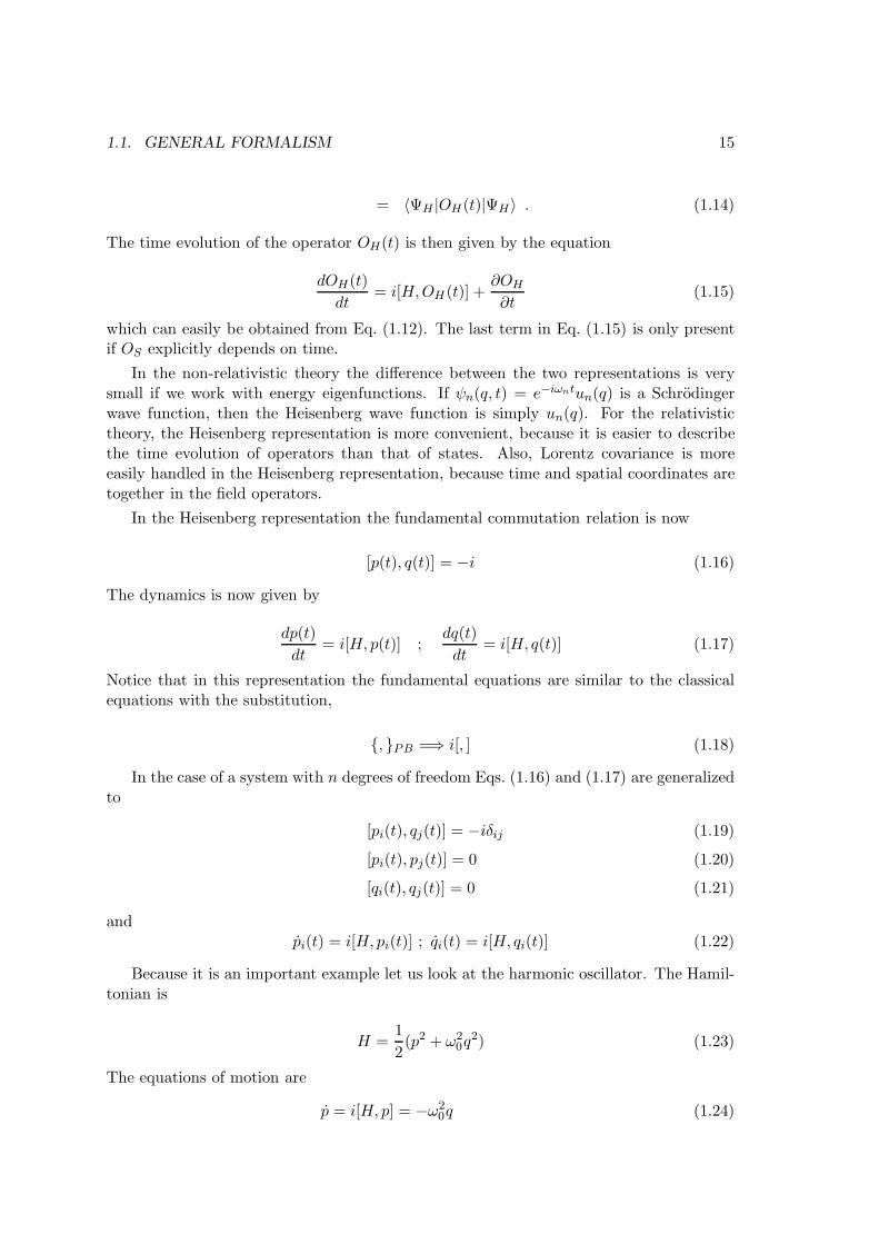
∆F (k) is the propagator in momenta space (Fourier transform). The equivalence be-tween Eq. (1.164) and Eq. (1.163) is done using integration in the complex plane of thetime component k0, with the help of the residue theorem. The contour is defined by theiε prescription, as indicated in Fig. (1.1). Applying the operator (⊔⊓′x+m2) to ∆F (x
′−x)in any of the forms of Eq. (1.163) one can show that
(⊔⊓′x +m2)∆F (x′ − x) = −iδ4(x′ − x) (1.166)
that is, ∆F (x′ − x) is the Green’s function for the Klein-Gordon equation with Feynman
boundary conditions.
In the presence of interactions, Feynman propagator looses the simple form of Eq. (1.165).However, as we will see, the free propagator plays a key role in perturbation theory.

32 CHAPTER 1. FREE FIELD QUANTIZATION
Re k0
Im k0
Figure 1.1: Integration in the complex k0 plane.
1.3 Second quantization of the Dirac field
Let us now apply the formalism of second quantization to the Dirac field. As we willsee, something has to be changed, otherwise we would be led to a theory obeying Bosestatistics, while we know that electrons have spin 1/2 and obey Fermi statistics.
1.3.1 Canonical formalism for the Dirac field
The Lagrangian density that leads to the Dirac equation is
L = iψγµ∂µψ −mψψ (1.167)
The conjugate momentum to ψα is
πα =∂L∂ψα
= iψ†α (1.168)
while the conjugate momentum to ψ†α vanishes. The Hamiltonian density is then
H = πψ − L = ψ†(−i~α · ~∇+ βm)ψ (1.169)
The requirement of translational and Lorentz invariance for L leads to the tensors T µν
and Mµνλ. Using the obvious generalizations of Eqs. (1.75) and (1.79) we get
T µν = iψγµ∂νψ − gµνL (1.170)
and
Mµνλ = iψγµ(xν∂λ − xλ∂ν + σνλ)ψ −(xνgµλ − xµgνλ
)L (1.171)
where
σνλ =1
4[γν , γλ] (1.172)
The 4-momentum Pµ and the angular momentum tensor Mνλ are then given by,
Pµ ≡∫d3xT 0µ

1.3. SECOND QUANTIZATION OF THE DIRAC FIELD 33
Mµλ ≡∫d3xM0νλ (1.173)
or
H ≡∫d3xψ†(−i~α · ~∇+ βm)ψ
~P ≡∫d3xψ†(−i~∇)ψ (1.174)
If we define the angular momentum vector ~J ≡ (M23,M31,M12) we get
~J =
∫d3xψ†
(~r × 1
i~∇+
1
2~Σ
)ψ (1.175)
which has the familiar aspect ~J = ~L + ~S. We can also identify a conserved current,∂µj
µ = 0, with jµ = ψγµψ, which will give the conserved charge
Q =
∫d3xψ†ψ (1.176)
All that we have done so far is at the classical level. To apply the canonical formalismwe have to enforce commutation relations and verify the Lorentz invariance of the theory.This will lead us into problems. To see what are the problems and how to solve them, wewill introduce the plane wave expansions,
ψ(x) =
∫dp∑
s
[b(p, s)u(p, s)e−ip·x + d†(p, s)v(p, s)eip·x
](1.177)
ψ†(x) =∫dp∑
s
[b†(p, s)u†(p, s)e+ip·x + d(p, s)v†(p, s)e−ip·x
](1.178)
where u(p, s) and v(p, s) are the spinors for positive and negative energy, respectively,introduced in the study of the Dirac equation and b, b†, d and d† are operators. To seewhat are the problems with the canonical quantization of fermions, let us calculate Pµ.We get
Pµ =
∫dk kµ
∑
s
[b†(k, s)b(k, s) − d(k, s)d†(k, s)
](1.179)
where we have used the orthogonality and closure relations for the spinors u(p, s) andv(p, s). From Eq. (1.179) we realize that if we define the vacuum as b(k, s) |0〉 = d(k, s) |0〉 =0 and if we quantize with commutators then particles b and particles d will contribute withopposite signs to the energy and the theory will not have a stable ground state. In fact,this was the problem already encountered in the study of the negative energy solutions ofthe Dirac equation, and this is the reason for the negative sign in Eq. (1.179). Dirac’s holetheory required Fermi statistics for the electrons and we will see how spin and statisticsare related.
To discover what are the relations that b, b†, d and d† should obey, we recall that atthe quantum level it is always necessary to verify Lorentz invariance. This gives,
i[Pµ, ψ(x)] = ∂µψ ; i[Pµ, ψ(x)] = ∂µψ (1.180)

34 CHAPTER 1. FREE FIELD QUANTIZATION
Instead of imposing canonical quantization commutators and, as a consequence, verifyingEq. (1.180) we will do the other way around. We start with Eq. (1.180) and we willdiscover the appropriate relations for the operators. Using the expansions Eqs. (1.177)and (1.178) we can show that Eq. (1.180) leads to
[Pµ, b(k, s)] = −kµb(k, s) ; [Pµ, b†(k, s)] = kµb
†(k, s) (1.181)
[Pµ, d(k, s)] = −kµd(k, s) ; [Pµ, d†(k, s)] = kµd
†(k, s) (1.182)
Using Eq. (1.179) for Pµ we get
∑
s′
[(b†(p, s′)b(p, s′)− d(p, s′)d†(p, s′)
), b(k, s)
]= −(2π)32k0δ3(~k − ~p)b(k, s) (1.183)
and three other similar relations. If we assume that
[d†(p, s′)d(p, s′), b(k, s)] = 0 (1.184)
the condition from Eq. (1.183) reads
∑
s′
[b†(p, s′)b(p, s′), b(k, s) − b†(p, s′), b(k, s)b(p, s′)
]=
= −(2π)32k0δ3(~p− ~k)b(k, s) (1.185)
where the parenthesis , denote anti-commutators. It is easy to see that Eq. (1.185) isverified if we impose the canonical commutation relations. We should have
b†(p, s), b(k, s) = (2π)32k0δ3(~p − ~k)δss′
d†(p, s′), d(k, s) = (2π)32k0δ3(~p− ~k)δss′ (1.186)
and all the other anti-commutators vanish. Note that as b anti-commutes with d and d†,then it commutes with d†d and therefore Eq. (1.184) is verified.
With the anti-commutator relations both contributions to Pµ in Eq. (1.179) are posi-tive. As in boson case we have to subtract the zero point energy. This is done, as usual,by taking all quantities normal ordered. Therefore we have for Pµ,
Pµ =
∫dk kµ
∑
s
:(b†(k, s)b(k, s) − d(k, s)d†(k, s)
):
=
∫dk kµ
∑
s
:(b†(k, s)b(k, s) + d†(k, s)d(k, s)
): (1.187)
and for the charge
Q =
∫d3x : ψ†(x)ψ(x) :
=
∫dk∑
s
[b†(k, s)b(k, s) − d†(k, s)d(k, s)
](1.188)

1.3. SECOND QUANTIZATION OF THE DIRAC FIELD 35
which means that the quanta of b type have charge +1 while those of d type have charge−1. It is interesting to note that was the second quantization of the Dirac field thatintroduced the − sign in Eq. (1.188), making the charge operator without a definite sign,while in Dirac theory was the probability density that was positive defined. The reverseis true for bosons. We can easily show that
[Q, b†(k, s)] = b†(k, s) [Q, d(k, s)] = d(k, s)
[Q, b(k, s)] = −b(k, s) [Q, d†(k, s)] = −d†(k, s)and then
[Q,ψ] = −ψ ; [Q,ψ] = ψ (1.189)
In QED the charge is given by eQ (e < 0). Therefore we see that ψ creates positrons andannihilates electrons and the opposite happens with ψ.
We can introduce the number operators
N+(p, s) = b†(p, s)b(p, s) ; N−(p, s) = d†(p, s)d(p, s) (1.190)
and we can rewrite
Pµ =
∫dk kµ
∑
s
(N+(k, s) +N−(k, s)) (1.191)
Q =
∫dk∑
s
(N+(k, s)−N−(k, s)) (1.192)
Using the anti-commutator relations in Eq. (1.186) it is now easy to verify that the theoryis Lorentz invariant, that is (see Problem 1.4),
i[Mµν , ψ] = (xµ∂ν − xν∂µ)ψ +Σµνψ . (1.193)
1.3.2 Microscopic causality
The anti-commutation relations in Eq. (1.186) can be used to find the anti-commutationrelations at equal times for the fields. We get
ψα(~x, t), ψ†β(~y, t) = δ3(~x− ~y)δαβ (1.194)
andψα(~x, t), ψβ(~y, t) = ψ†α(~x, t), ψ†β(~y, t) = 0 (1.195)
These relations can be generalized to unequal times
ψα(x), ψ†β(y) =
∫dp[[(p/+m)γ0
]αβ
e−ip·(x−y) −[(−p/+m)γ0
]αβ
eip·(x−y)]
=[(i∂/x +m)γ0
]αβ
i∆(x− y) (1.196)
where the ∆(x− y) function was defined in Eq. (1.128) for the scalar field. The fact thatγ0 appears in Eq. (1.196) is due to the fact that in Eq. (1.196) we took ψ† and not ψ. Infact, if we multiply on the right by γ0 we get
ψα(x), ψβ(y) = (i∂/x +m)αβi∆(x− y) (1.197)

36 CHAPTER 1. FREE FIELD QUANTIZATION
and
ψα(x), ψβ(y) = ψα(x), ψβ(y) = 0 (1.198)
We can easily verify the covariance of Eq. (1.197). We use
U(a, b)ψ(x)U−1(a, b) = S−1(a)ψ(ax + b)
U(a, b)ψ(x)U−1(a, b) = ψ(ax+ b)S(a)
S−1γµS = aµνγν (1.199)
to get
U(a, b)ψα(x), ψβ(y)U−1(a, b) =
= S−1ατ (a)ψτ (ax+ b), ψλ(ay + b)Sλβ(a)
= S−1ατ (a)(i∂/ax +m)τλi∆(ax− ay)Sλβ(a)
= (i∂/ +m)αβi∆(x− y) (1.200)
where we have used the invariance of ∆(x − y) and the result S−1i∂/axS = i∂/x. For(x − y)2 < 0 the anti-commutators vanish, because ∆(x − y) also vanishes. This resultallows us to show that any two observables built as bilinear products of ψ e ψ commutefor two spacetime points for which (x− y)2 < 0. Therefore
[ψα(x)ψβ(x), ψλ(y)ψτ (y)
]=
= ψα(x)ψβ(x), ψλ(y)ψτ (y)− ψα(x), ψλ(y)ψβ(x)ψτ (y)
+ψλ(y)ψα(x)ψβ(x), ψτ (y) − ψλ(y)ψτ (y), ψα(x)ψβ(x)
= 0 (1.201)
for (x− y)2 < 0. In this way the microscopic causality is satisfied for the physical observ-ables, such as the charge density or the momentum density.
1.3.3 Feynman propagator
For the Dirac field, as in the case of the charged scalar field, there are two ways of increasingthe charge by one unit in x′ and decrease it by one unit in x (note that the electron hasnegative charge). These ways are
θ(t′ − t)⟨0|ψβ(x′)ψ†α(x)|0
⟩(1.202)
θ(t− t′)⟨0|ψ†α(x)ψβ(x′)|0
⟩(1.203)
In Eq. (1.202) an electron of positive energy is created at ~x in the instant t, propagatesuntil ~x′ where is annihilated at time t′ > t. In Eq. (1.203) a positron of positive energyis created in x′ and annihilated at x with t > t′. The Feynman propagator is obtained

1.4. ELECTROMAGNETIC FIELD QUANTIZATION 37
summing the two amplitudes. Due the exchange of ψβ and ψα there must be a minus signbetween these two amplitudes. Multiplying by γ0, in order to get ψ instead of ψ†, we getfor the Feynman propagator,
SF (x′ − x)αβ = θ(t′ − t)
⟨0|ψα(x′)ψβ(x)|0
⟩
−θ(t− t′)⟨0|ψβ(x)ψα(x′)|0
⟩
≡⟨0|Tψα(x′)ψβ(x)|0
⟩(1.204)
where we have defined the time ordered product for fermion fields,
Tη(x)χ(y) ≡ θ(x0 − y0)η(x)χ(y) − θ(y0 − x0)χ(y)η(x) . (1.205)
Inserting in Eq. (1.204) the expansions for ψ and ψ we get,
SF (x′ − x)αβ=
∫dk[(k/ +m)αβθ(t
′ − t)e−ik·(x′−x) + (−k/+m)αβθ(t− t′)eik·(x
′−x)]
=
∫d4k
(2π)4i(k/ +m)αβk2 −m2 + iε
e−ik·(x′−x)
≡∫
d4k
(2π)4SF (k)αβe
−ik·(x′−x) (1.206)
where SF (k) is the Feynman propagator in momenta space. We can also verify thatFeynman’s propagator is the Green function for the Dirac equation, that is (see Problem1.7),
(i∂/−m)λα SF (x′ − x)αβ = iδλβδ
4(x′ − x) (1.207)
1.4 Electromagnetic field quantization
1.4.1 Introduction
The free electromagnetic field is described by the classical Lagrangian,
L = −1
4FµνF
µν (1.208)
where
Fµν = ∂µAν − ∂νAµ (1.209)
The free field Maxwell equations are
∂αFαβ = 0 (1.210)
that corresponds to the usual equations in 3-vector notation,
~∇ · ~E = 0 ; ~∇× ~B =∂ ~E
∂t(1.211)

38 CHAPTER 1. FREE FIELD QUANTIZATION
The other Maxwell equations are a consequence of Eq. (1.209) and can written as,
∂αFαβ = 0 ; Fαβ =
1
2εαβµνFµν (1.212)
corresponding to
~∇ · ~B = 0 ; ~∇× ~E = −∂~B
∂t(1.213)
Classically, the quantities with physical significance are the fields ~E e ~B, and thepotentials Aµ are auxiliary quantities that are not unique due to the gauge invariance ofthe theory. In quantum theory the potentials Aµ are the ones playing the leading roleas, for instance in the minimal prescription. We have therefore to formulate the quantumfields theory in terms of Aµ and not of ~E and ~B.
When we try to apply the canonical quantization to the potentials Aµ we immediatelyrun into difficulties. For instance, if we define the conjugate momentum as,
πµ =∂L∂(Aµ)
(1.214)
we get
πk =∂L
∂(Ak)= −Ak − ∂A0
∂xk= Ek
π0 =∂L∂A0
= 0 (1.215)
Therefore the conjugate momentum to the coordinate A0 vanishes and does not allowus to use directly the canonical formalism. The problem has its origin in the fact that thephoton, that we want to describe, has only two degrees of freedom (positive or negativehelicity) but we are using a field Aµ with four degrees of freedom. In fact, we have toimpose constraints on Aµ in such a way that it describes the photon. This problem canbe addressed in three different ways:
i) Radiation Gauge
Historically, this was the first method to be used. It is based in the fact that it isalways possible to choose a gauge, called the radiation gauge, where
A0 = 0 ; ~∇ · ~A = 0 (1.216)
that is, the potential ~A is transverse. The conditions in Eq. (1.216) reduce the num-ber of degrees of freedom to two, the transverse components of ~A. It is then possibleto apply the canonical formalism to these transverse components and quantize theelectromagnetic field in this way. The problem with this method is that we looseexplicit Lorentz covariance. It is then necessary to show that this is recovered in thefinal result. This method is followed in many text books, for instance in Bjorkenand Drell [1].

1.4. ELECTROMAGNETIC FIELD QUANTIZATION 39
ii) Quantization of systems with constraints
It can be shown that the electromagnetism is an example of an Hamilton generalizedsystem, that is a system where there are constraints among the variables. The wayto quantize these systems was developed by Dirac for systems of particles with ndegrees of freedom. The generalization to quantum field theories is done using theformalism of path integrals. We will study this method in Chapter 6, as it will beshown, this is the only method that can be applied to non-abelian gauge theories,like the Standard Model.
iii) Undefined metric formalism
There is another method that works for the electromagnetism, called the formalismof the undefined metric, developed by Gupta and Bleuler [2, 3]. In this formalism,that we will study below, Lorentz covariance is kept, that is we will always workwith the 4-vector Aµ, but the price to pay is the appearance of states with negativenorm. We have then to define the Hilbert space of the physical states as a sub-spacewhere the norm is positive. We see that in all cases, in order to maintain the explicitLorentz covariance, we have to complicate the formalism. We will follow the bookof Silvan Schweber [4].
1.4.2 Undefined metric formalism
To solve the difficulty of the vanishing of π0, we will start by modifying the MaxwellLagrangian introducing a new term,
L = −1
4FµνF
µν − 1
2ξ(∂ ·A)2 (1.217)
where ξ is a dimensionless parameter. The equations of motion are now,
⊔⊓Aµ −(1− 1
ξ
)∂µ(∂ ·A) = 0 (1.218)
and the conjugate momenta
πµ =∂L∂Aµ
= Fµ0 − 1
ξgµ0(∂ ·A) (1.219)
that is π0 = −1
ξ (∂ ·A)πk = Ek
We remark that the Lagrangian of Eq. (1.216) and the equations of motion, Eq. (1.218),reduce to Maxwell theory in the gauge ∂ · A = 0. This why we say that the choice ofEq. (1.216) corresponds to a class of Lorenz gauges with parameter ξ. With this abuse oflanguage (in fact we are not setting ∂ · A = 0, otherwise the problems would come back)the value of ξ = 1 is known as the Feynman gauge and ξ = 0 as the Landau gauge.
From Eq. (1.218) we get⊔⊓(∂ ·A) = 0 (1.220)

40 CHAPTER 1. FREE FIELD QUANTIZATION
implying that (∂ ·A) is a massless scalar field. Although it would be possible to continuewith a general ξ, from now on we will take the case of the so-called Feynman gauge, whereξ = 1. Then the equation of motion coincide with the Maxwell theory in the Lorenz gauge.As we do not have anymore π0 = 0, we can impose the canonical commutation relationsat equal times:
[πµ(~x, t), Aν(~y, t)] = −igµν δ3(~x− ~y)
[Aµ(~x, t), Aν(~y, t)] = [πµ(~x, t), πν(~y, t)] = 0 (1.221)
Knowing that [Aµ(~x, t), Aµ(~y, t)] = 0 at equal times, we can conclude that the spacederivatives of Aµ also commute at equal times. Then, noticing that
πµ = −Aµ + space derivatives (1.222)
we can write instead of Eq. (1.221)
[Aµ(~x, t), Aν(~y, t)] = [Aµ(~x, t), Aµ(~y, t)] = 0
[Aµ(~x, t), Aν(~y, t)] = igµνδ3(~x− ~y) (1.223)
If we compare these relations with the corresponding ones for the real scalar field, wherethe only one non-vanishing is,
[ϕ(~x, t), ϕ(~y, t)] = −iδ3(~x− ~y) (1.224)
we see (gµν = diag(+,−,−,−) that the relations for space components are equal but theydiffer for the time component. This sign will be the source of the difficulties previouslymentioned.
If, for the moment, we do not worry about this sign, we expand Aµ(x) in plane waves,
Aµ(x) =
∫dk
3∑
λ=0
[a(k, λ)εµ(k, λ)e−ik·x + a†(k, λ)εµ∗(k, λ)eik·x
](1.225)
where εµ(k, λ) are a set of four independent 4-vectors that we assume to real, without lossof generality. We will now make a choice for these 4-vectors. We choose εµ(1) and εµ(2)orthogonal to kµ and nµ, such that
εµ(k, λ)εµ(k, λ′) = −δλλ′ for λ, λ′ = 1, 2 (1.226)
After, we choose εµ(k, 3) in the plane (kµ, nµ) orthogonal to nµ and normalized, that is
εµ(k, 3)nµ = 0 ; εµ(k, 3)εµ(k, 3) = −1 (1.227)
Finally we choose εµ(k, 0) = nµ. The vectors εµ(k, 1) and εµ(k, 2) are called transversepolarizations, while εµ(k, 3) and εµ(k, 0) longitudinal and scalar polarizations, respec-tively. We can give an example. In the frame where nµ = (1, 0, 0, 0) and ~k is along the zaxis we have
εµ(k, 0) ≡ (1, 0, 0, 0) ; εµ(k, 1) ≡ (0, 1, 0, 0)

1.4. ELECTROMAGNETIC FIELD QUANTIZATION 41
εµ(k, 2) ≡ (0, 0, 1, 0) ; εµ(k, 3) ≡ (0, 0, 0, 1) (1.228)
In general we can show that
ε(k, λ) · ε∗(k, λ′) = gλλ′
∑
λ
gλλεµ(k, λ)ε∗ν (k, λ) = gµν (1.229)
Inserting the expansion (1.225) in (1.223) we get
[a(k, λ), a†(k′, λ′)] = −gλλ′2k0(2π)3δ3(~k − ~k′) (1.230)
showing, once more, that the quanta associated with λ = 0 has a commutation relationwith the wrong sign. Before addressing this problem, we can verify that the generalizationof Eq. (1.223) for arbitrary times is
[Aµ(x), Aν(y)] = −igµν∆(x, y) (1.231)
showing the covariance of the theory. The function ∆(x− y) is the same that was intro-duced before for scalar fields.
Therefore, up to this point, everything is as if we had 4 scalar fields. There is, however,the problem of the sign difference in one of the commutators. Let us now see what arethe consequences of this sign. For that we introduce the vacuum state defined by
a(k, λ) |0〉 = 0 λ = 0, 1, 2, 3 (1.232)
To see the problem with the sign we construct the one-particle state with scalar polariza-tion, that is
|1〉 =∫dk f(k)a†(k, 0) |0〉 (1.233)
and calculate its norm
〈1|1〉 =
∫dk1dk2f
∗(k1)f(k2)⟨0|a(k1, 0)a†(k2, 0)|0
⟩
= −〈0|0〉∫dk |f(k)|2 (1.234)
where we have used Eq. (1.230) for λ = 0. The state |1〉 has a negative norm. Thesame calculation for the other polarization would give well behaved positive norms. Wetherefore conclude that the Fock space of the theory has indefinite metric. What happensthen to the probabilistic interpretation of quantum mechanics?
To solve this problem we note that we are not working anymore with the classicalMaxwell theory because we modified the Lagrangian. What we would like to do is toimpose the condition ∂ · A = 0, but that is impossible as an equation for operators, asthat would bring us back to the initial problems with π0 = 0. We can, however, requirethat condition on a weaker form, as a condition only to be verified by the physical states.

42 CHAPTER 1. FREE FIELD QUANTIZATION
More specifically, we require that the part of ∂ ·A that contains the annihilation operator(positive frequencies) annihilates the physical states,
∂µA(+)µ |ψ〉 = 0 (1.235)
The states |ψ〉 can be written in the form
|ψ〉 = |ψT 〉 |φ〉 (1.236)
where |ψT 〉 is obtained from the vacuum with creation operators with transverse polar-ization and |φ〉 with scalar and longitudinal polarization. This decomposition depends,of course, on the choice of polarization vectors. To understand the consequences of
Eq. (1.235) is enough to analyze the states |φ〉 as ∂µA(+)µ contains only scalar and longi-
tudinal polarizations,
i∂ · A(+) =
∫dk e−ik·x
∑
λ=0,3
a(k, λ) ε(k, λ) · k (1.237)
and therefore Eq. (1.235) becomes
∑
λ=0,3
k · ε(k, λ) a(k, λ) |φ〉 = 0 (1.238)
Condition (1.238) does not determine completely |φ〉. In fact, there is much arbitrari-ness in the choice of the transverse polarization vectors, to which we can always add aterm proportional to kµ because k · k = 0. This arbitrariness must reflect itself on thechoice of |φ〉. Condition (1.238) is equivalent to,
[a(k, 0) − a(k, 3)] |φ〉 = 0 . (1.239)
We can construct |φ〉 as a linear combination of states |φn〉 with n scalar or longitudinalphotons:
|φ〉 = C0 |φ0〉+ C1 |φ1〉+ · · ·+ Cn |φn〉+ · · ·
|φ0〉 ≡ |0〉 (1.240)
The states |φn〉 are eigenstates of the operator number for scalar or longitudinal pho-tons,
N ′ |φn〉 = n |φn〉 (1.241)
where
N ′ =∫dk[a†(k, 3)a(k, 3) − a†(k, 0)a(k, 0)
](1.242)
Thenn 〈φn|φn〉 =
⟨φn|N ′|φn
⟩= 0 (1.243)
where we have used Eq. (1.239). This means that
〈φn|φn〉 = δn0 (1.244)

1.4. ELECTROMAGNETIC FIELD QUANTIZATION 43
that is, for n 6= 0, the state |φn〉 has zero norm. We have then for the general state |φ〉,〈φ|φ〉 = |C0|2 ≥ 0 (1.245)
and the coefficients Ci, i = 1, · · · n · · · are arbitrary. We have to show that this arbitrarinessdoes not affect the physical observables. The Hamiltonian is
H =
∫d3x : πµAµ − L :
=1
2
∫d3x :
3∑
i=1
[A2i + (~∇Ai)2
]− A2
0 − (~∇A0)2 :
=
∫dk k0
[3∑
λ=1
a†(k, λ)a(k, λ) − a†(k, 0)a(k, 0)
](1.246)
It is easy to check that if |ψ〉 is a physical state we have
〈ψ|H|ψ〉〈ψ|ψ〉 =
⟨ψT |
∫dk k0
∑2λ=1 a
†(k, λ)a(k, λ)|ψT⟩
〈ψT |ψT 〉(1.247)
and the arbitrariness on the physical states completely disappears when we take averagevalues. Besides that, only the physical transverse polarizations contribute to the result.One can show (see Problem 1.10) that the arbitrariness in |φ〉 is related with a gaugetransformation within the class of Lorenz gauges.
It is important to note that although for the average values of the physical observablesonly the transverse polarizations contribute, the scalar and longitudinal polarizations arenecessary for the consistency of the theory. In particular they show up when we considercomplete sums over the intermediate states.
Invariance for translations is readily verified. For that we write,
Pµ =
∫dk kµ
3∑
λ=0
(−gλλ)a†(k, λ)a(k, λ) (1.248)
Then
i[Pµ, Aν ] =
∫dk dk
′ikµ∑
λ,λ′
(−gλλ)[a†(k, λ)a(k, λ), a(k′ , λ′)
]εν(k′, λ′)e−ik·x
+[a†(x, λ)a(k, λ), a†(k′, λ′)
]ε∗ν(k′, λ′)eik
′·x
=
∫dk ikµ
∑
λ
[a(k, λ)εν(k, λ)e−ik·x − a†(k, λ)εν(k, λ)eik·x
]
= ∂µAν (1.249)
showing the invariance under translations. In a similar way, it can be shown the invariancefor Lorentz transformations (see Problem 1.11). For that we have to show that
M jk =
∫d3x :
[xjT 0k − xkT 0j + EjAk − EkAj
]: (1.250)

44 CHAPTER 1. FREE FIELD QUANTIZATION
M0i =
∫d3x :
[x0T 0i − xiT 00 − (∂ ·A)Ai − EiA0
]: (1.251)
where (ξ = 1)
T 0i = −(∂ ·A) ∂iA0 − Ek∂iAk
T 00 =
3∑
i=1
[A2i + (~∇Aj)2
]− A2
0 − (~∇A0)2 (1.252)
Using these expressions one can show that the photon has helicity ±1, correspondingtherefore to spin one. For that we start by choosing the direction of ~k along the axis 3(z axis) and take the polarization vector with the choice of Eq. (1.228). A one-photonphysical state will then be (not normalized),
|k, λ〉 = a†(k, λ) |0〉 λ = 1, 2 (1.253)
Let us now calculate the angular momentum along the axis 3. This is given by
M12 |k, λ〉 = M12a†(k, λ) |0〉
= [M12, a†(k, λ)] |0〉 (1.254)
where we have used the fact that the vacuum state satisfiesM12 |0〉 = 0. The operatorM12
has one part corresponding the orbital angular momenta and another corresponding to thespin. The contribution of the orbital angular momenta vanishes (angular momenta in thedirection of motion) as one can see calculating the commutator. In fact the commutatorwith the orbital angular momenta is proportional to k1 or k2, which are zero by hypothesis.Let us then calculate the spin part. Using the notation,
Aµ = Aµ(+) +Aµ(−) (1.255)
where Aµ(+)(Aµ(−)) correspond to the positive (negative) frequencies, we get
: E1A2−E2A1 := E1(+)A2(+)+E1(−)A2(+)+A2(−)E1(+)+E1(−)A2(−)− (1 ↔ 2) (1.256)
Then[: E1A2 − E2A1 :, a†(k, λ)
]=
= E1(+)[A2(+), a†(k, λ)
]+[E1(+), a†(k, λ)
]A2(+)
+E1(−)[A2(+), a†(k, λ)
]+A2(−)
[E1(+), a†(k, λ)
]− (1 ↔ 2)
= E1[A2(+), a†(k, λ)
]+A2
[E1(+), a†(k, λ)
]− (1 ↔ 2) (1.257)
Now (recall that λ = 1, 2)
[A2(+), a†(k, λ)]=∫dk′∑
λ′
ε2(k′, λ′)[a(k′, λ′), a†(k, λ)
]e−ik
′·x

1.4. ELECTROMAGNETIC FIELD QUANTIZATION 45
=ε2(k, λ)e−ik·x
[E1(+), a†(k, λ)]=∫dk′∑
λ′
(ik′0ε0(k′, λ′) + ik′1ε0(k′, λ′)
) [a(k′, λ′), a†(k, λ)
]e−ik
′·x
= ik0ε1(k, λ)e−ik·x (1.258)
Therefore∫d3x
[: E1A2 − E2A1 :, a†(k, λ)
]
=
∫d3xe−ik·x
[E1ε2(k, λ) +A2ik0ε1(k, λ) − E2ε1(k, λ) +A1ik0ε2(k, λ)
]
=
∫d3xe−ik·x
[ε1(k, λ)∂
↔0A
2(x)− ε2(k, λ)∂↔
0A1(x)
](1.259)
where we have used the fact that Ei = −Ai, i = 1, 2, for our choice of frame andpolarization vectors. On the other hand
a(k, λ) = −i∫d3xeik·x ∂
↔0 ε
µ(k, λ)Aµ(x)
a†(k, λ) = i
∫d3xe−ik·x ∂
↔0 ε
µ(k, λ)Aµ(x) (1.260)
For our choice we get
a†(k, 1) = −i∫d3xe−ik·x ∂
↔0 A
1(x)
a†(k, 2) = −i∫d3xe−ik·x ∂
↔0 A
2(x) (1.261)
and therefore[M12, a†(k, λ)] = iε1(k, λ)a†(k, 2) − iε2(k, λ)a†(k, 1) (1.262)
We find that the state a†(k, λ) |0〉 , λ = 1, 2 is not an eigenstate of the operator M12.However the linear combinations,
a†R(k) =1√2
[a†(k, 1) + ia†(k, 2)
]
a†L(k) =1√2
[a†(k, 1) − ia†(k, 2)
](1.263)
which correspond to right and left circular polarization, verify
[M12, a†R(k)] = a†R(k) ; [M12, a†L(k)] = −a†L(k) (1.264)
showing that the photon has spin 1 with right or left circular polarization (negative orpositive helicity).

46 CHAPTER 1. FREE FIELD QUANTIZATION
1.4.3 Feynman propagator
The Feynman propagator is defined as the vacuum expectation value of the time orderedproduct of the fields, that is
Gµν(x, y) ≡ 〈0|TAµ(x)Aν(y)|0〉
= θ(x0 − y0) 〈0|Aµ(x)Aν(y)|0〉 + θ(y0 − x0) 〈0|Aν(y)Aµ(x)|0〉 (1.265)
Inserting the expansions for Aµ(x) and Aν(y) we get
Gµν(x− y) = −gµν∫dk[e−ik·(x−y)θ(x0 − y0) + eik·(x−y)θ(y
0−x0)]
= −gµν∫
d4k
(2π)4i
k2 + iεe−ik·(x−y)
≡∫
d4k
(2π)4Gµν(k)e
−ik·(x−y) (1.266)
where Gµν(k) is the Feynman propagator on the momentum space
Gµν(k) ≡−igµνk2 + iε
(1.267)
It is easy to verify that Gµν(x− y) is the Green’s function of the equation of motion, thatfor ξ = 1 is the wave equation, that is
⊔⊓xGµν(x− y) = igµνδ4(x− y) (1.268)
These expressions for Gµν(x−y) and Gµν(k) correspond to the particular case of ξ = 1,the so-called Feynman gauge. For the general case where ξ 6= 0 the equation of motionreads [
⊔⊓xgµρ −(1− 1
ξ
)∂µ∂ρ
]Aρ(x) = 0 (1.269)
For this case the equal times commutation relations are more complicated (see Problem1.12). Using those relations one can show that the Feynman propagator is still the Green’sfunction of the equation of motion, that is
[⊔⊓xgµρ −
(1− 1
ξ
)∂µ∂ρ
]〈0|TAρ(x)Aν(y)|0〉 = igµνδ4(x− y) (1.270)
Using this equation we can then obtain in an arbitrary ξ gauge (of the Lorenz type),
Gµν(k) = −i gµνk2 + iε
+ i(1− ξ)kµkν
(k2 + iε)2. (1.271)
1.5. DISCRETE SYMMETRIES 47
1.5 Discrete Symmetries
We know from the study of the Dirac equation the transformations like space inversion(Parity) and charge conjugation, are symmetries of the Dirac equation. More precisely, ifψ(x) is a solution of the Dirac equation, then
ψ′(x) = ψ′(−~x, t) = γ0ψ(~x, t) (1.272)
ψc(x) = CψT(x) (1.273)
are also solutions (if we take the charge −e for ψc). Similar operations could also bedefined for scalar and vector fields.
With second quantization the fields are no longer functions, they become operators. Wehave therefore to find unitary operators P and C that describe those operations within thisformalism. There is another discrete symmetry, time reversal, that in second quantizationwill be described by an anti-unitary operator T . We will exemplify with the scalar fieldhow to get these operators. We will leave the Dirac and Maxwell fields as exercises.
1.5.1 Parity
To define the meaning of the Parity operation we have to put the system in interactionwith the measuring system, considered to be classical. This means that we will considerthe system described by
L −→ L− jµ(x)Aµext(x) (1.274)
where we have considered that the interaction is electromagnetic. jµ(x) is the electromag-netic current that has the form,
jµ(x) = ie : ϕ∗∂↔µϕ : scalar field
jµ(x) = e : ψγµψ : Dirac field (1.275)
In a Parity transformation we invert the coordinates of the measuring system, thereforethe classical fields are now
Aµext = (A0ext(−~x, t)),− ~Aext(−~x, t) = Aextµ (−~x, t) (1.276)
For the dynamics of the new system to be identical to that of the original system, whichshould be the case if Parity is conserved, it is necessary that the equations of motionremain the same. This is true if
PL(~x, t)P−1 = L(−~x, t) (1.277)
Pjµ(~x, t)P−1 = jµ(−~x, t) (1.278)
Eqs. (1.277) and (1.278) are the conditions that a theory should obey in order to beinvariant under Parity. Furthermore P should leave the commutation relations unchanged,so that the quantum dynamics is preserved. For each theory that conserves Parity shouldbe possible to find an unitary operator P that satisfies these conditions.

48 CHAPTER 1. FREE FIELD QUANTIZATION
Now we will find such an operator P for the scalar field. It is easy to verify that thecondition
Pϕ(~x, t)P−1 = ±ϕ(−~x, t) (1.279)
satisfies all the requirements. The sign ± is the intrinsic parity of the particle describedby the field ϕ, (+ for scalar and − for pseudo-scalar). In terms of the expansion of themomentum, Eq. (1.279) requires
Pa(k)P−1 = ±a(−k) ; Pa†(k)P−1 = ±a†(−k) (1.280)
where −k means that we have changed ~k into −~k (but k0 remains intact, that is, k0 =
+
√|~k|2 +m2). It is easier to solve Eq. (1.280) in the momentum space. As P should be
unitary, we writeP = eiP (1.281)
Then
Pa(k)P−1 = a(k) + i[P, a(k)] + · · ·+ in
n![P, [· · · , [P, a(k)] · · · ] + · · ·
= −a(−k) (1.282)
where we have chosen the case of the pseudo-scalar field.
Eq. (1.282) suggests the form
[P, a(k)] =λ
2[a(k) + εa(−k)] (1.283)
where λ and ε = ±1 are to be determined. We get
[P, [P, a(k)]] =λ2
2[a(k) + εa(−k)] (1.284)
and therefore
Pa(k)P−1 = a(k) +1
2
[iλ+
(iλ)2
2!+ · · · + (iλ)4
n!+ · · ·
](a(k) + εa(−k))
=1
2[a(k) − εa(−k)] + 1
2eiλ[a(k) + εa(−k)]
= −a(−k) (1.285)
We solve Eq. (1.285) if we choose λ = π and ε = +1 (λ = π and ε = −1 for the scalarcase). It is easy to check that
Pps = −π2
∫dk[a†(k)a(k) + a†(k)a(−k)
]= P †ps (1.286)
and it is solution of Eq. (1.283) for λ = π and ε = +1. Therefore,
Pps = exp
−iπ
2
∫dk[a†(k)a(k) + a†(k)a(−k)
](1.287)

1.5. DISCRETE SYMMETRIES 49
and for the scalar field
Ps = exp
−iπ
2
∫dk[a†(k)a(k) − a†(k)a(−k)
](1.288)
For the case of the Dirac field, the condition equivalent to Eq. (1.279) is now
Pψ(~x, t)P−1 = γ0ψ(−~x, t) (1.289)
Repeating the same steps we get
PDirac = exp
−iπ
2
∫dp∑
s
[b†(p, s)b(p, s)− b†(p, s)b(−p, s)
+ d†(p, s)d(p, s) + d†(p, s)d(−p, s)]
(1.290)
The case of the Maxwell field is left as an exercise.
1.5.2 Charge conjugation
The conditions for charge conjugation invariance are now
CL(x)C−1 = L ; CjµC−1 = −jµ (1.291)
where jµ is the electromagnetic current. Conditions (1.291) are verified for the chargedscalar fields if
Cϕ(x)C−1 = ϕ∗(x) ; Cϕ∗(x)C−1 = ϕ(x) (1.292)
and for the Dirac field if
Cψα(x)C−1 = Cαβ ψβ(x)
Cψα(x)C−1 = −ψβ(x)C−1βα (1.293)
where C is the charge conjugation matrix.
Finally from the invariance of jµAµ we obtain the condition for the electromagnetic
field,
CAµC−1 = −Aµ (1.294)
By using a method similar to the one used in the case of the Parity we can get theoperator C for the different theories. For instance, for the scalar field we get
Cs = exp
iπ
2
∫dk (a†+ − a†−)(a+ − a−)
(1.295)
and for the Dirac field
C = C1C2 (1.296)

50 CHAPTER 1. FREE FIELD QUANTIZATION
with
C1 = exp
−i∫dp∑
s
φ(p, s)[b†(p, s)b(p, s)− d†(p, s)d(p, s)
]
C2 = exp
iπ
2
∫dp∑
s
[b†(p, s)− d†(p, s)
][b(p, s)− d(p, s)]
(1.297)
with
v(p, s) = eiφ(p,s) uc(p, s)
u(p, s) = eiφ(p,s) vc(p, s) (1.298)
where the phase φ(p, s) is arbitrary (see [5]).
1.5.3 Time reversal
Classically the meaning of the time reversal invariance it is clear. We change the sign ofthe time, the velocities change direction and the system goes from what was the final stateto the initial state. This exchange between the initial and final state has as consequence, inquantum mechanics, that the corresponding operator must be anti-linear or anti-unitary.In fact 〈f |i〉 = 〈i|f〉∗ and therefore if we want 〈T ϕf |T ϕi〉 = 〈ϕi|ϕf 〉 then T must includethe complex conjugation operation. We can write
T = UK (1.299)
where U is unitary and K is the instruction to tale the complex conjugate of all c-numbers.Then
〈Tϕf |Tϕi〉 = 〈UKϕf |UKϕi〉
= 〈Uϕf |Uϕi〉∗
= 〈ϕf |ϕi〉∗ = 〈ϕi|ϕf 〉 (1.300)
as we wanted. A theory will be invariant under time reversal if
T L(~x, t)T −1 = L(~x,−t)
T jµ(~x, t)T −1 = jµ(~x,−t) (1.301)
For the scalar field this condition will be verified if
T ϕ(~x, t)T −1 = ±ϕ(~x,−t) (1.302)
and for the electromagnetic field we must have.
T Aµ(~x, t)T −1 = Aµ(~x,−t) (1.303)

1.5. DISCRETE SYMMETRIES 51
making jµAµ invariant. For the case of the Dirac field the transformation is
T ψα(~x, t)T −1 = Tαβψβ(~x,−t) (1.304)
In order that Eq. (1.301) is satisfied, the T matrix must satisfy
TγµT−1 = γTµ = γµ∗ (1.305)
with a solution, in the Dirac representation,
T = iγ1γ3 (1.306)
Applying the same type of reasoning already used for P and C we can find T , orequivalently, U . For the Dirac field, noticing that
Tu(p, s) = u∗(−p,−s)eiα+(p,s)
Tv(p, s) = v∗(−p,−s)eiα−(p,s) (1.307)
we can write U = U1U2 and obtain
U1 = exp
−i∫dp∑
s
[α+b
†(p, s)b(p, s)− α−d†(p, s)d(p, s)
](1.308)
and
U2 = exp
−iπ
2
∫dp∑
s
[b†(p, s)b(p, s) + b†(p, s)b(−p− s)
− d†(p, s)d(p, s) − d†(p, s)d(−p,−s)]
(1.309)
1.5.4 The T CP theorem
It is a fundamental theorem in Quantum Field Theory that the product T CP is an invari-ance of any theory that satisfies the following general conditions:
• The theory is local and covariant for Lorentz transformations.
• The theory is quantized using the usual relation between spin and statistics, that is,commutators for bosons and anti-commutators for fermions.
This theorem due to Ludus, Zumino, Pauli e Schwinger has an important consequencethat if one of the discrete symmetries is not preserved then another one must also beviolated to preserve the invariance of the product. For a proof of the theorem see thebooks of Bjorken and Drell[1, 6] and Itzykson and Zuber[7].

52 CHAPTER 1. FREE FIELD QUANTIZATION
Problems for Chapter 1
1.1 Verify, for the scalar field, the covariant relations for translations and Lorentz trans-formations,
i[Pµ, ϕ] = ∂µϕ
i[Mµν , ϕ] = (xµ∂ν − xν∂µ)ϕ (1.310)
1.2 Show that
∂0∆(x− y)|x0=y0 = −δ3(~x− ~y) (1.311)
1.3 Show that
∫d4k
(2π)4i
k2 −m2 + iεe−ik·(x−y) =
=
∫dk[θ(x0 − y0)e−ik·(x−y) + θ(y0 − x0)eik·(x−y)
](1.312)
where dk ≡ d3k
(2π)32k0. Hint: Integrate in the complex plane of the variable dk0 and use
the prescription iε to define the contours.
1.4 Show that for the Dirac theory the requirements of Lorentz invariance are satisfied,
i[Mµν , ϕ] = (xµ∂ν − xν∂µ)ϕ+Σµνϕ ; Σµν =1
4[γµ, γν ] (1.313)
1.5 Show that
ψα(~x, t), ψ†β(~y, t) = δαβδ3(~x− ~y) (1.314)
1.6 Show that
SF (x− y)αβ = θ(x0 − y0)⟨0|ψα(x)ψβ(y)|0
⟩
−θ(y0 − x0)⟨0|ψβ(y)ψα(x)|0
⟩(1.315)
corresponds to

Problems 53
SF (x− y)αβ =
∫d4p
(2π)4i(p/+m)αβp2 −m2 + iε
e−ip·(x−y) (1.316)
Hint: Expand ψα e ψβ in plane waves.
1.7 Show that(i∂/x −m)αβSF (x− y)βγ = iδαγδ
4(x− y) (1.317)
1.8 Show that is is always possible to choose the electromagnetic potential Aµ such that
A0 = 0 , ~∇ · ~A = 0 (Radiation gauge) (1.318)
1.9 Show that we have[Aµ(x), Aν(y)] = −igµν∆(x− y) (1.319)
1.10 Consider the indefinite metric formalism for the electromagnetic field.
a) Consider the expectation value of Aµ in the state |φ〉. Show that
〈φ|Aµ|φ〉 = C∗0C1
∫dk e−ik·x 〈0| [εµ(k, 3)a(k, 3) + εµ(k, 0)a(k, 0)] |φ1〉
+h.c. (1.320)
b) Choose the state |φ1〉 in the form
|φ1〉 =∫dk f(k)
[a†(k, 3) − a†(k, 0)
]|0〉 (1.321)
Show that
〈φ|Aµ|φ〉 =∫dk [εµ(k, 3) + εµ(k, 0)] (C
∗0C1e
−ik·xf(k) + c.c.) (1.322)
c) Choose εµ(k, λ) to be real. Show that
εµ(k, 3) + εµ(k, 0) =kµ
(n · k) (1.323)
d) Show that
〈φ|Aµ|φ〉 = ∂µΛ(x) (1.324)
where
⊔⊓Λ = 0 (1.325)
Comment the result.
54 CHAPTER 1. FREE FIELD QUANTIZATION
1.11 Show the covariance of the electromagnetism for the Lorentz transformations,
i[Mµν , Aλ] = (xµ∂ν − xν∂µ)Aλ +Σµν,λσAσ (1.326)
whereΣµν,λσ = gµλgνσ − gµσgλν (1.327)
1.12 Show that for the general case of ξ 6= 1 we have
[Aµ(~x, t), Aν(~y, t)] = 0
[Aµ(~x, t), Aν(~y, t)] = igµν [1− (1− ξ)gµ0] δ3(~x− ~y)
[Ai(~x, t), Aj(~y, t)] = [A0(~x, t), A0(~y, t)] = 0
[A0(~x, t), Ai(~y, t)] = i(1− ξ)∂iδ3(~x− ~y) (1.328)
1.13 Use the results of Problem 1.12 to show that, in the general gauge with ξ 6= 1 wehave [
⊔⊓xgµρ −(1− 1
ξ
)∂µ∂ρ
]〈0|TAρ(x)Aν(y)|0〉 = igµνδ4(x− y) (1.329)
where (⊔⊓gµρ−
(1− 1
ξ
)∂µ∂ρ
)Aρ = 0 (1.330)
1.14 Find the operator P for the Dirac and Maxwell fields.
1.15 Find the operator C for the Dirac and Maxwell fields.
1.16 Show thatT ψα(~x, t)T−1 = Tαβψβ(~x,−t) (1.331)
ensures thatT L(~x, t)T −1 = L(~x,−t) (1.332)
if there is a matrix T such that TγµT−1 = γµ∗. Find T in the Dirac representation.
1.17 Find the operator T for the Dirac and Maxwell fields.
1.18 Consider the Lagrangian
L = ψiγµDµPLψ −mψψ (1.333)
where
Dµ = ∂µ + iAaµτa
2
PL =1− γ5
2(1.334)
Show that the theory is neither invariant under P nor under C but it is invariant for theproduct CP .

Chapter 2
Physical States. S Matrix. LSZReduction.
2.1 Physical states
In the previous chapter we saw, for the case of free fields, how to construct the space ofstates, the so-called Fock space of the theory. When we consider the real physical case,with interactions, we are no longer able to solve the problem exactly. For instance, theinteraction between electrons and photons is given by a set of nonlinear coupled equations,
(i∂/−m)ψ = eA/ ψ
∂µFµν = eψγνψ (2.1)
that do not have an exact solution. In practice we have to resort to approximation meth-ods. In the following chapter we will learn how to develop a covariant perturbation theory.Here we are going just to study the general properties of the theory.
Let us start by the physical states. As we do not know how to solve the problem exactly,we can not prove the assumptions we are going to make about these states. However, theseare reasonable assumptions, based essentially on Lorentz covariance. We choose our statesto be eigenstates of energy and momentum, and of all the other observables that commutewith Pµ. Besides that, we will also assume that
i) The eigenvalues of p2 are non-negative and p0 > 0.
ii) There exists one non-degenerate base state, with the minimum of energy, which isLorentz invariant. This state is called the vacuum state |0〉 and by convention
pµ |0〉 = 0 (2.2)
iii) There exist one particle states∣∣p(i)
⟩, such that,
p(i)µ p(i)µ = m2
i (2.3)
55

56 CHAPTER 2. PHYSICAL STATES. S MATRIX. LSZ REDUCTION.
for each stable particle with mass mi.
iv) The vacuum and the one-particle states constitute the discrete spectrum of pν.
2.2 In states
As we are mainly interested in scattering problems, we should construct states that havea simple interpretation in the limit t → −∞. At that time, the particles that are goingto participate in the scattering process have not interacted yet (we assume that the in-teractions are adiabatically switched off when |t| → ∞ which is appropriate for scatteringproblems).
We look for operators that create one particle states with the physical mass. To beexplicit, we start by an hermitian scalar field given by the Lagrangian
L =1
2∂µϕ∂µϕ− 1
2m2ϕ2 − V (x) (2.4)
where V (x) is an operator made of more than two interacting fields ϕ at point x. Forinstance, those interactions can be self-interactions of the type
V (x) =λ
4!ϕ4(x) (2.5)
The field ϕ satisfies the following equation of motion
(⊔⊓+m2)ϕ(x) = − ∂V
∂ϕ(x)≡ j(x) (2.6)
and the equal time canonical commutation relations,
[ϕ(~x, t)ϕ(~y, t)] = [π(~x, t)π(~y, t)] = 0
[π(~x, t), ϕ(~y, t)] = −iδ3(~x− ~y) (2.7)
whereπ(x) = ϕ(x) (2.8)
if we assume that V (x) has no derivatives. We designate by ϕin(x) the operator thatcreates one-particle states. It will be a functional of the fields ϕ(x). Its existence will beshown by explicit construction. We require that ϕin(x) must satisfy the conditions:
i) ϕin(x) and ϕ(x) transform in the same way for translations and Lorentz transforma-tions. For translations we have then
i [Pµ, ϕin(x)] = ∂µϕin(x) (2.9)
ii) The spacetime evolution of ϕin(x) corresponds to that of a free particle of mass m,that is
(⊔⊓+m2)ϕin(x) = 0 (2.10)

2.2. IN STATES 57
From these definitions it follows that ϕin(x) creates one-particle states from the vac-uum. In fact, let us consider a state |n〉, such that,
Pµ |n〉 = pµn |n〉 . (2.11)
Then
∂µ 〈n|ϕin(x)|0〉 = i 〈n| [Pµ, ϕin(x)] |0〉
= ipµn 〈n|ϕin(x)|0〉 (2.12)
and therefore⊔⊓ 〈n|ϕin(x)|0〉 = −p2n 〈n|ϕin(x)|0〉 (2.13)
Then(⊔⊓ +m2) 〈n|ϕin(x)|0〉 = (m2 − p2n) 〈n|ϕin(x)|0〉 = 0 (2.14)
where we have used the fact that ϕin(x) is a free field, Eq. (2.10). Therefore the statescreated from the vacuum by ϕin are those for which p2n = m2, that is, the one-particlestates of mass m.
The Fourier decomposition of ϕin(x) is then the same as for free fields, that is,
ϕin(x) =
∫dk[ain(k)e
−ik·x + a†in(k)eik·x]
(2.15)
where ain(k) and a†in(k) satisfy the usual algebra for creation and annihilation operators.
In particular, by repeated use of a†in(k) we can create one state of n particles.
To express ϕin(x) in terms of ϕ(x) we start by introducing the retarded Green’s func-tion of the Klein-Gordon operator,
(⊔⊓x +m2)∆ret(x− y;m) = δ4(x− y) (2.16)
where∆ret(x− y;m) = 0 if x0 < y0 (2.17)
We can then write
√Zϕin(x) = ϕ(x)−
∫d4y∆ret(x− y;m)j(y) (2.18)
The field ϕin(x), defined by Eq. (2.15), satisfies the two initial conditions. The constant√Z was introduced to normalize ϕin in such a way that it has amplitude 1 to create
one-particle states from the vacuum. The fact that ∆ret = 0 for x0 → −∞, suggests that√Zϕin(x) is, in some way, the limit of ϕ(x) when x0 → −∞. In fact, as ϕ and ϕin are
operators, the correct asymptotic condition must be set on the matrix elements of theoperators. Let |α〉 and |β〉 be two normalized states. We define the operators
ϕf (t) = i
∫d3xf∗(x) ∂
↔0 ϕ(x)
ϕfin = i
∫d3xf∗(x) ∂
↔0 ϕin(x) (2.19)

58 CHAPTER 2. PHYSICAL STATES. S MATRIX. LSZ REDUCTION.
where f(x) is a normalized solution of the Klein-Gordon equation. By Green’s theorem,
ϕfin does not depend on time (for plane waves f = e−ik·x and ϕfin = ain). Then theasymptotic condition of Lehmann, Symanzik e Zimmermann (LSZ) [8], is
limt→−∞
〈α|ϕf (t) |β〉 =√Z 〈α|ϕfin |β〉 (2.20)
2.3 Spectral representation for scalar fields
We saw that Z had a physical meaning as the square of the amplitude for the field ϕ(x)to create one-particle states from the vacuum. Let us now find a formal expression for Zand show that 0 ≤ Z ≤ 1.
We start by calculating the expectation value in the vacuum of the commutator of twofields,
i∆′(x, y) ≡ 〈0| [ϕ(x), ϕ(y)] |0〉 (2.21)
As we do not know how to solve the equations for the interacting fields ϕ, we can not solveexactly the problem of finding the ∆′, in contrast with the free field case. We can, however,determine its form using general arguments of Lorentz invariance and the assumed spectrafor the physical states. We introduce a complete set of states between the two operatorsin Eq. (2.21) and we use the invariance under translations in order to obtain,
〈n|ϕ(y)|m〉 = 〈n| eiP ·yϕ(0)e−iP ·y |m〉
= ei(pn−pm)·y 〈n|ϕ(0)|m〉 (2.22)
Therefore we get
∆′(x, y) = −i∑
n
〈0|ϕ(0)|n〉 〈n|ϕ(0)|0〉 (e−ipn·(x−y) − eipn·(x−y))
≡ ∆′(x− y) (2.23)
that is, like in the free field case, ∆′ is only a function of the difference x− y. Introducingnow
1 =
∫d4q δ4(q − pn) (2.24)
we get
∆′(x− y) = −i∫
d4q
(2π)3
[(2π)3
∑
n
δ4(pn − q)| 〈0|ϕ(0)|n〉 |2](e−iq·(x−y) − eiq·(x−y))
= −i∫
d4q
(2π)3ρ(q)(e−iq·(x−y) − eiq·(x−y)) (2.25)
where we have defined the density ρ(q) (spectral amplitude),
ρ(q) = (2π)3∑
n
δ4(pn − q)| 〈0|ϕ(0)|n〉 |2 (2.26)

2.3. SPECTRAL REPRESENTATION FOR SCALAR FIELDS 59
This spectral amplitude measures the contribution to ∆′ of the states with 4-momentumqµ. ρ(q) is Lorentz invariant (as can be shown using the invariance of ϕ(x) and theproperties of the vacuum and of the states |n〉) and vanishes when q is not in future lightcone, due the assumed properties of the physical states. Then we can write
ρ(q) = ρ(q2)θ(q0) (2.27)
and we get
∆′(x− y) = −i∫
d4q
(2π)3ρ(q2)θ(q0)(e−iq·(x−y) − eiq·(x−y))
= −i∫
d4q
(2π)3
∫dσ2δ(q2 − σ2)ρ(σ2)θ(q0)
[e−iq·(x−y) − eiq·(x−y)
]
=
∫ ∞
0dσ2ρ(σ2)∆(x− y;σ) (2.28)
where
∆(x− y;σ) = −i∫
d4q
(2π)3δ(q2 − σ2)θ(q0)(e−iq·(x−y) − eiq·(x−y)) (2.29)
is the invariant function defined for the commutator of free fields with mass σ.
The Eq. (2.28) is known as the spectral decomposition of the commutator of two fields.This expression will allow us to show that 0 ≤ Z < 1. To show that, we separate the statesof one-particle from the sum in Eq. (2.26). Let |p〉 be a one-particle state with momentump. Then
〈0|ϕ(x)|p〉 =√Z 〈0|ϕin(x)|p〉+
∫d4y∆ret(x− y;m) 〈0|j(y)|p〉
=√Z 〈0|ϕin(x)|p〉 (2.30)
where we have used
〈0|j(y)|p〉 =⟨0|(⊔⊓ +m2)ϕ(y)|p
⟩=
= (⊔⊓+m2)e−ip·y 〈0|ϕ(0)|p〉
= (m2 − p2)e−ip·y 〈0|ϕ(0)|p〉 = 0 (2.31)
On the other hand
〈0|ϕin(x)|p〉 =
∫d3k
(2π)32ωke−ik·x 〈0|ain(k)|p〉
= e−ip·x (2.32)
and therefore
ρ(q) = (2π)3∫dp δ4(p − q)Z + contributions from more than one particle

60 CHAPTER 2. PHYSICAL STATES. S MATRIX. LSZ REDUCTION.
= Zδ(q2 −m2)θ(q0) + · · · (2.33)
Therefore
∆′(x− y) = Z∆(x− y;m) +
∫ ∞
m21
dσ2ρ(σ2)∆(x− y;σ) (2.34)
where m1 is the mass of the lightest state of two or more particles. Finally noticing that
∂
∂x0∆′(x− y)|x0=y0 =
∂
∂x0∆(x− y;σ)|x0=y0 = −δ3(~x− ~y) (2.35)
we get the relation
1 = Z +
∫ ∞
m21
dσ2ρ(σ2) (2.36)
which means0 ≤ Z < 1 (2.37)
where this last step results from the assumed positivity of ρ(σ2).
2.4 Out states
In the same way as we reduced the dynamics of t → −∞ to the free fields ϕin, it is alsopossible to define in the limit t → +∞ the corresponding free fields, ϕout(x). These freefields will be the final state of a scattering problem. The formalism is copied from thecase of ϕin, and therefore we will present the results without going into the details of thederivations. ϕout(x) obey the following relations:
i [Pµ, ϕout] = ∂µϕout
(⊔⊓+m2)ϕout = 0 (2.38)
and has the expansion
ϕout(x) =
∫dk[aout(k)e
−ik·x + a†out(k)eik·x]
(2.39)
The asymptotic condition is now
limt→∞
〈α|ϕf (t) |β〉 =√Z 〈α|ϕfout |β〉 (2.40)
and √Zϕout(x) = ϕ(x) −
∫d4y∆adv(x− y;m)j(y) (2.41)
where the Green’s functions ∆adv satisfy
(⊔⊓x +m2)∆adv(x− y;m) = δ4(x− y)
∆adv(x− y;m) = 0 ; x0 > y0 . (2.42)
For one-particle states we get
〈0|ϕ(x)|p〉 =√Z 〈0|ϕout(x)|p〉
=√Z 〈0|ϕin(x)|p〉
=√Ze−ip·x (2.43)
2.5. S MATRIX 61
2.5 S matrix
We have now all the formalism needed to study the transition amplitudes from one initialstate to a given final state, the so-called S matrix elements. Let us start by an initial statewith n non-interacting particles (we suppose that initially they are well separated),
|p1 · · · pn ; in〉 ≡ |α ; in〉 (2.44)
where p1 · · · pn are the 4-momenta of the n particles. Other quantum numbers are assumedbut not explicitly written. The final state will be, in general, a state with m particles
∣∣p′1 · · · p′m ; out⟩≡ |β ; out〉 (2.45)
The S matrix element Sβα is defined by the amplitude
Sβα ≡ 〈β ; out|α ; in〉 (2.46)
The S matrix is an operator that induces an isomorphism between the in and out states,that by assumption are a complete set of states,
〈β ; out| = 〈β ; in|S
〈β ; in| = 〈β ; out|S−1
〈β ; out|α ; in〉 = 〈β ; in|S|α ; in〉 = 〈β ; out|S|α; out〉 (2.47)
From the assumed properties for the states we can show the following results for theS matrix.
i) 〈0|S|0〉 = 〈0|0〉 = 1 (stability and unicity of the vacuum)
ii) The stability of the one-particle states gives
〈p ; in|S|p ; in〉 = 〈p ; out|p ; in〉 = 〈p ; in|p ; out〉 = 1 (2.48)
because |p ; in〉 = |p ; out〉.
iii) ϕin(x) = Sϕout(x)S−1
iv) The S matrix is unitary. To show this we have
δβα = 〈β ; out|α ; out〉 =⟨β ; in|SS†|α ; in
⟩(2.49)
and therefore
SS† = 1 (2.50)

62 CHAPTER 2. PHYSICAL STATES. S MATRIX. LSZ REDUCTION.
v) The S matrix is Lorentz invariant. In fact we have
ϕin(ax+ b) = U(a, b)ϕin(x)U−1(a, b) = USϕout(x)S
−1U−1
= USU−1ϕout(ax+ b)US−1U−1 . (2.51)
But
ϕin(ax+ b) = Sϕout(ax+ b)S−1 , (2.52)
and therefore we get finally
S = U(a, b)SU−1(a, b) . (2.53)
2.6 Reduction formula for scalar fields
The S matrix elements are the quantities that are directly connected to the experiment.In fact, |Sβα|2 represents the transition probability from the initial state |α ; in〉 to thefinal |β ; out〉. We are going in this section to use the previous formalism to express thesematrix elements in terms of the so-called Green functions for the interacting fields. Inthis way the problem of the calculation of these probabilities is transferred to the problemof calculating these Green functions. These, of course, can not be evaluated exactly, butwe will learn in the next chapter how to develop a covariant perturbation theory for thatpurpose.
Let us then proceed to the derivation of the relation between the S matrix elementsand the the Green functions of the theory. This technique is known as the LSZ reductionfrom the names of Lehmann, Symanzik e Zimmermann [8] that have introduced it. Bydefinition
〈p1 · · · ; out|q1 · · · ; in〉 =⟨p1, · · · ; out|a†in(q1)|q2, · · · ; in
⟩(2.54)
Using
a†in(q1) = −i∫
td3xe−iq1·x ∂
↔0ϕin(x) (2.55)
where the integral is time-independent, and therefore can be calculated for an arbitrarytime t. If we take t → −∞ and use the asymptotic condition for the in fields, Eq. (2.20),we get
〈p1 · · · ; out|q1 · · · ; in〉 = − limt→−∞
iZ−1/2∫
td3xe−iq1·x ∂
↔0 〈p1 · · · ; out|ϕ(x)|q2 · · · ; in〉
(2.56)
In a similar way one can show that
⟨p1 · · · ; out|a†out(q1)|q2 · · · ; in
⟩=
2.6. REDUCTION FORMULA FOR SCALAR FIELDS 63
= − limt→∞
iZ−1/2∫
td3xe−iq1·x ∂
↔0 〈p1 · · · ; out|ϕ(x)|q2 · · · ; in〉 . (2.57)
Then, using the result,
(limt→∞
− limt→−∞
)∫d3xf(~x, t) = lim
tf→∞,ti→−∞
∫ tf
ti
dt∂
∂t
∫d3xf(~x, t)
=
∫d4x∂0f(~x, t) (2.58)
and subtracting Eq. (2.57) from Eq. (2.56) we get
〈p1 · · · ; out|q1 · · · ; in〉=⟨p1 · · · ; out|a†out(q1)|q2 · · · ; in
⟩
+iZ−1/2∫d4x ∂0
[e−iq1·x∂
↔0 〈p1 · · · ; out|ϕ(x)|q2 · · · ; in〉
](2.59)
The first term on the right-hand side of Eq. (2.59) corresponds to a sum of disconnectedterms, in which at least one of the particles is not affected by the interaction (it will vanishif none of the initial momenta coincides with one of the final momenta). Its form is
⟨p1 · · · ; out|a†out(q1)|q2 · · · ; in
⟩=
=n∑
k=1
(2π)32p0k δ3(~pk − ~q1) 〈p1, · · · , pk, · · · ; out|q2, · · · ; in〉 (2.60)
where pk means that this momentum was taken out from that state. For the second termwe write,
∫d4x ∂0
[e−iqix∂
↔0 〈p1 · · · ; out|ϕ(x)|q2 · · · ; in〉
]
=
∫d4x
[−∂20e−iq1·x 〈· · · 〉+ e−iq1·x∂20 〈· · · 〉
]
=
∫d4x
[(−∆2 +m2)e−iq1·x 〈· · · 〉+ e−iq1·x∂20 〈· · · 〉
]
=
∫d4xe−iq1·x(⊔⊓+m2) 〈p1 · · · ; out|ϕ(x)|q2 · · · ; in〉 (2.61)
where we have used (⊔⊓ + m2)e−iq1·x = 0, and have performed an integration by parts(whose justification would imply the substitution of plane waves by wave packets).
Therefore, after this first step in the reduction we get,
〈p1, · · · pn; out|q1 · · · qℓ; in〉 =
=n∑
k=1
2p0k(2π)3δ3(~pk − ~q1) 〈p1, · · · pk; · · · pn; out|q2 · · · q2 · · · qℓ; in〉

64 CHAPTER 2. PHYSICAL STATES. S MATRIX. LSZ REDUCTION.
+iZ−1/2∫d4xe−iq1x(⊔⊓+m2) 〈p1 · · · pn; out|ϕ(x)|q2 · · · qℓ; in〉 (2.62)
We will proceed with the process until all the momenta in the initial and final state areexchanged by the field operators. To be specific, let us now remove one momentum inthe final state. From now on we will no longer consider the disconnected terms, becausein practice we are only interested in the cases where all the particles interact1. We havethen
〈p1 · · · pn; out|ϕ(x1)|q2 · · · qℓ; in〉 = 〈p2 · · · pn; out|aout(p1)ϕ(x1)|q2 · · · qℓ; in〉
= limy01→∞
iZ−1/2∫d3y1 e
ip1·y1∂↔y01
〈p2 · · · pn; out|ϕ(y1)ϕ(x1)|q2 · · · qℓ; in〉
= 〈p2 · · · pn; out|ϕ(x1)ain(p1)|q2 · · · qℓ; in〉
+ limy01→∞
iZ−1/2∫d3y1 e
ip1·y1∂↔y01
〈p2 · · · pn; out|ϕ(y1)ϕ(x1)|q2 · · · qℓ; in〉
− limy01→−∞
iZ−1/2∫d3y1 e
ip1·y1∂↔y01
〈p2 · · · pn; out|ϕ(x1)ϕ(y1)|q2 · · · qℓ; in〉
= 〈p2 · · · pn; out|ϕ(x1)ain(p1)|q2 · · · qℓ; in〉
+iZ−1/2(
limy01→∞
− limy01→−∞
)∫d3y1 e
ip1·y1∂↔y01
〈p2 · · · pn; out|Tϕ(y1)ϕ(x1)|q2 · · · qℓ; in〉
(2.63)
where we have used the properties of the time-ordered product, Eq. (1.161). Applying thesame procedure that lead to Eq. (2.61) we obtain,
〈p1 · · · pn, ; out|ϕ(x1)|q2 · · · qℓ; in〉 = disconnected terms
+iZ−1/2∫d4y1e
ip1·y1(⊔⊓y1 +m2) 〈p2 · · · pn; out|Tϕ(y1)ϕ(x1)|q2 · · · qℓ; in〉 (2.64)
It is not very difficult to generalize this method to obtain the final reduction formulafor scalar fields,
〈p1 · · · pn; out|q1 · · · qℓ; in〉 = disconnected terms
+
(i√Z
)n+ℓ ∫d4y1 · · · d4ynd4x1 · · · d4xℓe[i
∑n1 pk·yk−i
∑ℓ1 qr ·xr]
(⊔⊓y1 +m2) · · · (⊔⊓xℓ +m2) 〈0|Tϕ(y1) · · ·ϕ(yn)ϕ(x1) · · ·ϕ(xℓ)|0〉 (2.65)
This last equation is the fundamental equation in quantum field theory. It allows us torelate the transition amplitudes to the Green functions of the theory. The quantity
〈0|Tϕ(x1) · · ·ϕ(xn)|0〉 ≡ G(x1 · · · xn) (2.66)
1Once we know the cases where all the particles interact, we can always calculate situations where someof the particles do not participate in the scattering.

2.7. REDUCTION FORMULA FOR FERMIONS 65
is known as the complete green function for r = m+ ℓ particles and we will introduce thefollowing diagrammatic representation for it,
G(x1 · · · xn) = (2.67)
x1 xi
xlxn
The factors (⊔⊓ +m2) in Eq. (2.65) force the external particles to be on-shell. In fact, inmomentum space (⊔⊓ + m2) → (−p2 +m2). Therefore, Eq. (2.65) will vanish unless thepropagators of the external legs are on-shell, as in that case they will have a pole, 1
p2−m2 .
Eq. (2.65) will then give the residue of that pole. We conclude that for the transitionamplitudes only the truncated Green functions will contribute, that is the ones with theexternal legs removed. In the next chapter we will learn how to evaluate these Greenfunctions in perturbation theory.
2.7 Reduction formula for fermions
2.7.1 States in and out
The definition of the in and out follows exactly the same steps as in the case of the scalarfields. We will therefore, for simplicity, just state the results with the details.
The states ψin(x) satisfy the conditions,
(i∂/−m)ψin(x) = 0
[Pµ, ψin(x)] = −i∂µψin(x) . (2.68)
The states ψin(x) will create one-particle states and they are related with the fields ψ(x)by, √
Z2ψin(x) = ψ(x)−∫d4ySret(x− y,m)j(y) (2.69)
where ψ(x) satisfies the Dirac equation,
(i∂/−m)ψ(x) = j(x) (2.70)
and Sret is the retarded Green function for the Dirac equation,
(i∂/x −m)Sret(x− y,m) = δ4(x− y)

66 CHAPTER 2. PHYSICAL STATES. S MATRIX. LSZ REDUCTION.
Sret(x− y) = 0 ; x0 < y0 (2.71)
The fields ψin(x), as free fields, have the Fourier expansion,
ψin(x) =
∫dp∑
s
[bin(p, s)u(p, s)e
−ip·x + d†in(p, s)v(p, s)eip·x]
(2.72)
where the operators bin, din satisfy exactly the same algebra as in the free field case. Theasymptotic condition is now,
limt→−∞
〈α|ψf (t) |β〉 =√Z2 〈α|ψfin |β〉 (2.73)
where ψf (t) and ψfin have a meaning similar to Eq. (2.19).
For the ψout fields we get essentially the same expressions with ψin substituted by ψout.The main difference is in the asymptotic condition that now reads,
limt→∞
〈α|ψf (t) |β〉 =√Z2 〈α|ψfout |β〉 (2.74)
implying the following relation between the fields ψout and ψ,
√Z2ψout = ψ(x) −
∫d4ySadv(x− y;m)j(y) (2.75)
where
(i∂/x −m)Sadv(x− y;m) = δ4(x− y)
Sadv(x− y;m) = 0 x0 > y0 . (2.76)
2.7.2 Spectral representation fermions
Let us consider the vacuum expectation value of the anti-commutator of two Dirac fields,
S′αβ(x, y) ≡ i 〈0| ψα(x), ψβ(y) |0〉
= i∑
n
[〈0|ψα(0) |n〉 〈n|ψβ(0) |0〉 e−ipn(x−y)
+ 〈0|ψβ(0) |n〉 〈n|ψα(0) |0〉 eipn·(x−y)]
≡ S′αβ(x− y) (2.77)
where we have introduced a complete set of eigen-states of the 4-momentum. As beforewe introduce the spectral amplitude ραβ(q),
ραβ(q) ≡ (2π)3∑
n
δ4(pn − q) 〈0|ψα(0) |n〉 〈n|ψβ(0) |0〉 (2.78)

2.7. REDUCTION FORMULA FOR FERMIONS 67
We will now find the most general form for ραβ(q) using Lorentz invariance arguments.ραβ(q) is a 4× 4 matrix in Dirac space, and can therefore be written as
ραβ(q) = ρ(q)δαβ + ρµ(q)γµαβ + ρµν(q)σ
µναβ + ρ(q)γ5αβ + ρµ(q)(γ
µγ5)αβ (2.79)
Lorentz invariance arguments restrict the form of the coefficients ρ(q), ρµ(q), ρµν(q), ρ(q)and ρµ(q). Under Lorentz transformations the fields transform as
U(a)ψα(0)U−1(a) = S−1αλ (a)ψλ(0)
U(a)ψα(0)U−1(a) = ψλ(0)Sλα(a)
S−1γµS = aµνγν (2.80)
Then we can show that the matrix (in Dirac space), ραβ must obey the relation,
ρ(q) = S−1(a)ρ(qa−1)S(a) (2.81)
where we have used a matrix notation. This relation gives the properties of the differentcoefficients on Eq. (2.79). For instance,
ρµ(q) = aµνρν(qa−1) (2.82)
which means that ρµ transform as a 4−vector.
Using the fact that ραβ is a function of q and vanishes outside the future light cone,we can finally write
ραβ(q) = ρ1(q2)q/αβ + ρ2(q
2)δαβ + ρ1(q2)(q/γ5)αβ + ρ2(q
2)γ5αβ (2.83)
that is, ραβ(q) is determined up to four scalar functions of q2. Requiring invariance underparity transformations we get, instead of Eq. (2.81),
ραβ(~q, q0) = γ0αλρλδ(−~q, q0)γ0δβ (2.84)
and inserting in Eq. (2.83) we obtain,
ρ1 = ρ2 = 0 (2.85)
Therefore for the Dirac theory, that preserves parity, we get,
ραβ(q) = ρ1(q2)q/αβ + ρ2(q
2)δαβ (2.86)
Repeating the steps of the scalar case we write,
S′αβ(x− y) =
∫ ∞
0dσ2
ρ1(σ
2)Sαβ(x− y;σ)+
+[σρ1(σ
2)− ρ2(σ2)]δαβ∆(x− y;σ)
(2.87)
where ∆ and Sαβ are the functions defined for free fields. We can then show that

68 CHAPTER 2. PHYSICAL STATES. S MATRIX. LSZ REDUCTION.
i) ρ1 e ρ2 are real
ii) ρ1(σ2) ≥ 0
iii) σρ1(σ2)− ρ2(σ
2) ≥ 0
Using the previous relations we can extract of the one-particle states from Eq. (2.87). Weget,
S′αβ(x− y) = Z2Sαβ(x− y;m)
+
∫ ∞
m21
dσ2ρ1(σ
2)Sαβ(x− y;σ)
+[σρ1(σ
2)− ρ2(σ2)]δαβ∆(x− y;σ)
(2.88)
where m1 is the threshold for the production of two or more particles. EvaluatingEq. (2.88) at equal times we can obtain
1 = Z2 +
∫
m21
dσ2ρ1(σ2) (2.89)
that is
0 ≤ Z2 < 1 (2.90)
2.7.3 Reduction formula fermions
To get the reduction formula for fermions we will proceed as in the scalar case. The onlydifficulty has to do with the spinor indices. The creation and annihilation operators canbe expressed in terms of the fields ψin by the relations,
bin(p, s) =
∫d3xu(p, s)eip·xγ0ψin(x)
d†in(p, s) =
∫d3xv(p, s)e−ip·xγ0ψin(x)
b†in(p, s) =
∫d3xψin(x)γ
0e−ip·xu(p, s)
din(p, s) =
∫d3xψin(x)γ
0eip·xv(p, s) (2.91)
with the integrals being time independent. In fact, to be more rigorous we should substi-tute the plane wave solutions by wave packets, but as in the scalar case, to simplify matterwe will not do it. To establish the reduction formula we start by extracting one electronfrom the initial state,
〈β; out|(ps)α; in〉 =⟨β; out|b†in(p, s)|α, in
⟩

2.7. REDUCTION FORMULA FOR FERMIONS 69
= 〈β − (p, s); out|α; in〉 +⟨β; out|b†in(p, s)− b†out(p, s)|α; in
⟩
= disconnected terms
+
∫d3x
⟨β; out|ψin(x)− ψout(x)|α; in
⟩γ0e−ip·xu(p, s)
= disconnected terms
−(
limt→+∞
− limt→−∞
)1√Z2
∫d3x
⟨β; out|ψ(x)|α; in
⟩γ0e−ip·xu(p, s)
= disconnected terms
−Z−1/22
∫d4x
[⟨β; out|∂0ψ(x)|α; in
⟩γ0e−ip·xu(p, s)
+⟨β; out|ψ(x)|α; in
⟩γ0∂0(e
−ip·xu(p, s))]
(2.92)
Using now(iγ0∂0 + iγi∂i −m)(e−ip·xu(p, s)) = 0 (2.93)
we get, after an integration by parts,
⟨β; out|b†in(ρ, s)|α; in
⟩= disconnected terms
−iZ−1/22
∫d4x
⟨β; out|ψ(x)|α; in
⟩(−i∂←/x −m)e−ip·xu(p, s) (2.94)
In a similar way the reduction of an anti-particle from the initial state gives,
⟨β; out|d†in(p, s)|α; in
⟩= disconnected terms
+iZ−1/22
∫d4xe−ip·xv(p, s)(i∂/x −m) 〈β; out|ψ(x)|α; in〉 (2.95)
while the reduction of a particle or of an anti-particle from the final state give, respectively,
〈β; out|bout(p, s)|α; in〉 = disconnected terms
−iZ−1/22
∫d4xeip·xu(p, s)(i∂/x −m) 〈β; out|ψ(x)|α; in〉 (2.96)
and
〈β; out|dout(p, s)|α; in〉 = disconnected terms
+iZ−1/22
∫d4x
⟨β; out|ψ(x)|α; in
⟩(−i∂←/x −m)v(p, s)eip·x (2.97)
Notice the formal relation between one electron in the initial state and a positron in thefinal state. To go from one to the other one just has to do,
u(p, s)e−ip·x → −v(p, s)eip·x (2.98)

70 CHAPTER 2. PHYSICAL STATES. S MATRIX. LSZ REDUCTION.
The following steps in the reduction are similar, one only has to pay attention to signsbecause of the anti-commutation relations for fermions. To write the final expression wedenote the momenta in the state 〈in| by pi or pi, respectively for particles or anti-particles,and those in the state 〈out| by p′i, p′i. We also make the following conventions (needed todefine the global sign),
|(p1, s1), · · · , (p1, s1); · · · ; in〉 = b†in(p1, s1) · · · d†in(p1, s1) · · · |0〉 (2.99)
and ⟨out; (p′1, s
′1) · · · , (p′1, s′1) · · ·
∣∣ = 〈0| · · · dout(p′1, s′1), · · · bout(p′1, s′1) (2.100)
Then, if n(n′) denotes the total number of particles (anti-particles), we get
⟨out; (p′1, s
′1) · · · , (p′1, s′1) · · · |(p1, s1), · · · (p1, s1), · · · ; in
⟩= disconnected terms
+(−iZ−1/22 )n(iZ−1/22 )n
′
∫d4x1 · · · d4y1 · · · d4x′1 · · · d4y′1 · · ·
e−i∑
(pi·xi)−i∑
(pi·yi)e+i∑
(p′i·x′i)+i∑
(p′i·y′i)
u(p′1, s′1)(i∂/x′1 −m) · · · v(p1, s1)(i∂/y1 −m)
〈0|T (· · ·ψ(y′1) · · ·ψ(x′1)ψ(x1) · · ·ψ(y1) · · · |0〉
(−i∂←/x1 −m)u(p1, s1) · · · (−i∂
←/y′1 −m)v(p′1, s
′1) (2.101)
Eq. (2.101) is the fundamental expression that allows to relate the elements of the Smatrix with the Green functions of the theory. The operators within the time-orderedproduct can be reordered, modulo some minus sign. The sign and ordering shown corre-spond to the conventions in Eqs. (2.99) and (2.100). In terms of diagrams, we representthe Green function,
〈0|T[ψ(y′m′) · · ·ψ(y′1)ψ(x′ℓ′) · · ·ψ(x′1)ψ(x1) · · ·ψ(xℓ)ψ(y1) · · ·ψ(ym)
]|0〉 (2.102)
by the diagram2 of Fig. (2.1).
The operators (i∂/−m) e (−i∂←/−m) force the particles to be on-shell and remove the
propagators from the external lines (truncated Green functions). In the next chapter wewill learn how to determine these functions in perturbation theory.
2.8 Reduction formula for photons
The LSZ formalism for photons, has some difficulties connected with the problems inquantizing the electromagnetic field. When one adopts a formalism (radiation gauge)
2With lepton number conservation, the number of particles minus anti-particles is conserved, that is
ℓ−m = ℓ′−m
′

2.8. REDUCTION FORMULA FOR PHOTONS 71
x1
x′1
y1
y′1
xl
x′l
ym
y′m
Figure 2.1: Green function for fermions.
where the only components of the field Aµ are transverse (as in Ref.[6]), the problemsarise in showing the Lorentz and gauge invariance of the S matrix. In the formalism ofthe undefined metric, that we adopted in section 1.4.2, the difficulties are connected withthe states of negative norm, besides the gauge invariance.
Here we are going to ignore these difficulties3 and assume that we can define the infields by the relation,
√Z3A
µin(x) = Aµ(x)−
∫d4yDµν
ret(x− y)jν(y) (2.103)
and in the same way for the out fields,
√Z3A
µout(x) = Aµ(x)−
∫d4yDµν
adv(x− y)jν(y) (2.104)
where
⊔⊓Aµin = ⊔⊓Aµout = 0
⊔⊓Aµ = jµ
⊔⊓Dµνadv, ret = δµνδµ(x− y) (2.105)
The fields in and out are free fields, and therefore they have a Fourier expansion inplane waves and creation and annihilation operators of the form
Aµin(x) =
∫dk
3∑
λ=0
[ain(k, λ)ε
µ(k, λ)e−ik·x + a†in(k, λ)εµ∗(k, λ)eik·x
](2.106)
and therefore
ain(k, λ) = −i∫d3xeik·x∂
↔0εµ(k, λ)Ainµ (x)
3We will see in chapter 6 a more satisfactory procedure to quantize all gauge theories, including Maxwelltheory of the electromagnetic field. We will see that the resulting perturbation theory coincides with theone we get here. This is our justification to be less precise here.

72 CHAPTER 2. PHYSICAL STATES. S MATRIX. LSZ REDUCTION.
a†in(k, λ) = i
∫d3xe−ik·x∂
↔0εµ∗(k, λ)Ainµ (x) (2.107)
where, as usual, ain(k, λ) and a†in(k, λ) are time independent. In Eq. (2.106) all thepolarizations appear, but as the elements of the S matrix are between physical states, weare sure that the longitudinal and scalar polarizations do not contribute. In this formalismwhat is difficult to show is the spectral decomposition. We are not going to enter thosedetails, just state that we can show that Z3 is gauge independent and satisfies 0 ≤ Z3 < 1.The reduction formula is easily obtained. We get
〈β; out|(kλ)α; in〉 = 〈β − (k, λ); out|α; in〉 +⟨β; out|a†in(k, λ) − a†out(k, λ)|α; in
⟩
= disconnected terms
+i
∫d3xe−ik·x∂
↔0ε∗µ(k, λ) 〈β; out|Aµin(x)−Aµout(x)|α; in〉
= disconnected terms
−i( limt→+∞
− limt→−∞
)Z−1/23
∫d3xe−ik·x∂
↔0 〈β; out|Aµ(x)|α; in〉 ε∗µ(k, λ)
= disconnected terms
−iZ−1/23
∫d4xe−ik·x∂
↔0 〈β; out|Aµ(x)|α; in〉 ε∗µ(k, λ)
= disconnected terms
−iZ−1/23
∫d4xe−ik·x~⊔⊓x 〈β; out|Aµ(x)|α; in〉 ε∗µ(k, λ) (2.108)
The final formula for photons is then⟨k′1 · · · k′n; out|k1 · · · kℓ; in
⟩= disconnected terms
+
( −i√Z3
)n+ℓ ∫d4y1 · · · d4ynd4x1 · · · d4xℓ e[i
∑n k′i·yi−i∑ℓ ki·xi]
εµ1(k1, λ1) · · · εµℓ(kℓ, λℓ)ε∗µ′1(k′1, λ
′1) · · · ε∗µ
′n(k′n, λ
′n)
⊔⊓y1 · · · ⊔⊓xℓ 〈0|T (Aµ′1(y1) · · ·Aµ′n(yn)Aµ1(x1) · · ·Aµℓ(xℓ) |0〉 (2.109)
and corresponds to the diagram of Fig. (2.2).
2.9 Cross sections
The reduction formulas, Eqs.(2.65), (2.101) and (2.109), are the fundamental results ofthis chapter. They relate the transition amplitudes from the initial to the final state withthe Green functions of the theory. In the next chapter we will show how to evaluate theseGreen functions setting up the so-called covariant perturbation theory. Before we closethis chapter, let us indicate how these transition amplitudes
Sfi ≡ 〈f ; out|i; in〉 (2.110)

2.9. CROSS SECTIONS 73
x1 xi
xlxn
Figure 2.2: Green function for photons.
are related with the quantities that are experimentally accessible, the cross sections. Thenthe path between experiment (cross sections) and theory (Green functions) will be estab-lished.
As we have seen in the reduction formulas there is always a trivial contribution to theS matrix, that corresponds to the so-called disconnected terms, when the system goes fromthe initial to the final state without interaction. The subtraction of this trivial contributionleads us to introduce the T matrix with the relation,
Sfi = 1fi − i(2π)4δ4(Pf − Pi)Tfi (2.111)
where we have factorized explicitly the delta function expressing the 4-momentum conser-vation. If we neglect the trivial contribution, the transition probability from the initial tothe final state will be given by
Wf←i =∣∣(2π)4δ4(Pf − Pi)Tfi
∣∣2 (2.112)
To proceed we have to deal with the meaning of a square of a delta function. Thisappears because we are using plane waves. To solve this problem we can normalize in abox of volume V and consider that the interaction has a duration of T . Then
(2π)4δ4(Pf − Pi) = limV → ∞T → ∞
∫
Vd3x
∫ T/2
−T/2dx0ei(Pf−Pi)·x . (2.113)
However
F ≡∫
Vd3x
∫ T/2
−T/2dx0ei(Pf−Pi)·x = V δ~Pf ~Pj
2
|Ef − Ei|sin
∣∣∣∣T
2(Ef − Ei)
∣∣∣∣ (2.114)
and the square of the last expression can be done, giving,
|F |2 = V 2δ~Pf , ~Pi4
|Ef − Ei|2sin2
∣∣∣∣T
2(Ef − Ei)
∣∣∣∣ . (2.115)
If we want the transition rate by unit of volume (and unit of time) we divide by V T . Then
Γfi = limV → ∞T → ∞
V δ~Pf , ~Pi 2sin2 T2 (Ef − Ei)T2 (Ef − Ei)2
|Tfi|2 (2.116)

74 CHAPTER 2. PHYSICAL STATES. S MATRIX. LSZ REDUCTION.
Using now the results
limV→∞
V δ~Pf ~Pj = (2π)3δ3(~Pf − ~Pi)
limT→∞
2sin2 T2 (Ef − Ei)T2 (Ef − Ei)2
= (2π) δ(Ef − Ei) (2.117)
we get for the transition rate by unit volume and unit time,
Γfi ≡ (2π)4δ4(Pf − Pi)|Tfi|2 (2.118)
To get the cross section we have to further divide by the incident flux, and normalize theparticle densities to one particle per unit volume. Finally, we sum (integrate) over all finalstates in a certain energy-momentum range. We get,
dσ =1
ρ1ρ2
1
|~v12|Γfi
n∏
j=3
d3pj2p0j(2π)
3(2.119)
whereρ1 = 2E1 ; ρ2 = 2E2 (2.120)
An equivalent way of writing this equation is
dσ =1
4[(pi · p2)2 −m2
1m22
]1/2 (2π)4δ4(Pf − Pi)|Tfi|2
n∏
j=3
dpj (2.121)
that exhibits well the Lorentz invariance of each part that enters the cross section4. Theincident flux and phase space factors are purely kinematics. The physics, with its inter-actions, is in the matrix element Tfi.
We note that with our conventions, fermion and boson fields have the same normal-ization, that is, the one-particle states obey
⟨p|p′⟩= 2p0(2π)3δ3(~p − ~p′) (2.122)
differing in this way from some older books like Ref.[1].
4It is assumed that, in the case of two beams they are in the same line. Then the cross section, beinga transverse area, is invariant for Lorentz transformations along that direction.

Problems 75
Problems for Chapter 2
2.1 Show that the spectral representation for fermions, ραβ(q), satisfies,
a) ρ(q) = S−1(a)ρ(qa−1)S(a)
b) ραβ(~q, q0) = γ0αλρλδ(−~q, q0)γ0δβ
2.2 Use the results of the previous problem to show that, in a theory that preserves Parity,like QED, we have
ραβ(q) = ρ1(q2)q/αβ + ρ2(q
2)δαβ (2.123)
2.3 Show that the functions ρ1 and ρ2 defined in problem 2.2 satisfy the following prop-erties:
i) ρ1 and ρ2 are real
ii) ρ1(σ2) ≥ 0
iii) σρ1(σ2)− ρ2(σ
2) ≥ 0
2.4 Show that for the Dirac field we have
1 = Z2 +
∫ ∞
m21
dσ2ρ1(σ2) (2.124)
2.5 Show that
〈0| [ϕin(x), ϕout(y)] |0〉 = i∆(x− y;m) (2.125)

76 CHAPTER 2. PHYSICAL STATES. S MATRIX. LSZ REDUCTION.
Chapter 3
Covariant Perturbation Theory
3.1 U matrix
In this chapter we are going to develop a method to evaluate the Green functions of agiven theory. From what we have seen in the two previous chapters, we realize that weonly know how to calculate for free fields, like the in an out fields. However, the Greenfunctions we are interested in, are given in terms of the physical interacting fields, and wedo not know how to operate with these. We are going to see how to express the physicalfields as perturbative series in terms of free in fields. In this way we will be able to evaluatethe Green functions in perturbation theory.
We start by defining the U matrix. To simplify matters, we will be considering, forthe moment, only scalar fields. In the end we will return to the other cases. The physicalinteracting fields ϕ(~x, t) and their conjugate momenta π(~x, t), satisfy the same equal timecommutation relations than the in fields, ϕin(~x, t) and their πin(~x, t). Also, both ϕ andϕin form a complete set of operators, in the sense that any state, free or interacting, canbe obtained by application of ϕin or ϕ in the vacuum. This implies that there should bean unitary transformation U(t) that relates ϕ with ϕin, that is,
ϕ(~x, t) = U−1(t)ϕin(~x, t)U(t)
π(~x, t) = U−1(t)πin(~x, t)U(t) (3.1)
The dynamics of U can be obtained from the equations of motion for ϕ(x) and ϕin(x).These are,
∂ϕin∂t
(x) = i[Hin(ϕin, πin), ϕin]
∂πin∂t
(x) = i[Hin(ϕin, πin), πin] (3.2)
and
∂ϕ
∂t(x) = i[H(ϕ, π), ϕ]
∂π
∂t(x) = i[H(ϕ, π), π] (3.3)
77

78 CHAPTER 3. COVARIANT PERTURBATION THEORY
Then from Eqs. (3.2) and (3.1) we get,
ϕin(x) =∂
∂t
[U(t)ϕ(x)U−1(t)
]
=[U(t)U−1(t), ϕin
]+ i [H(ϕin, πin), ϕin(x)]
= ϕin(x) +[UU−1 + iHI(ϕin, πin), ϕin
](3.4)
where
HI(ϕin, πin) = H(ϕin, πin)−Hin(ϕin, πin) ≡ HI(t) (3.5)
and in a similar way
πin(x) = πin +[UU−1 + iHI(ϕin, πin), πin
](3.6)
From Eqs. (3.4) and (3.6) we obtain,
iUU−1 = HI(t) + E0(t) (3.7)
where E0(t) commutes with ϕin and πin and is therefore a time dependent c-number, notan operator. Defining
H ′I(t) = HI(t) + E0(t) (3.8)
we get a differential equation for U(t), that reads,
i∂U(t)
∂t= H ′I(t)U(t) (3.9)
The solution of this equation in terms of the in fields, is the basis of the covariant pertur-bation theory.
To integrate Eq. (3.9) we need an initial condition. For that we introduce the operator
U(t, t′) ≡ U(t)U−1(t′) (3.10)
where t ≥ t′, and that obviously satisfies
U(t, t) = 1 (3.11)
It is easy to see that U(t, t′) also satisfies Eq. (3.9), that is,
i∂U(t, t′)
∂t= H ′I(t)U(t, t′) (3.12)
and has the initial condition, Eq. (3.11). To proceed we start by transforming Eq. (3.12)in an equivalent integral equation, that is,
U(t, t′) = 1− i
∫ t
t′dt1H
′I(t1)U(t1, t
′) (3.13)

3.1. U MATRIX 79
Notice that we have not solved the problem because U(t, t′) appears on both sides of theequation. However, we can iterate the equation to get the expansion,
U(t, t′) = 1− i
∫ t
t′dt1H
′I(t1) + (−i)2
∫ t
t′dt1H
′I(t1)
∫ t1
t′dt2H
′I(t2)
+ · · ·+ (−i)n∫ t
t′dt1
∫ t1
t′dt2 · · ·
∫ tn−1
t′dtnH
′I(t1) · · ·H ′I(tn)
+ · · · (3.14)
Of course this expansion can only be useful if HI contains a small parameter and, becauseof that, we can truncate the expansion at certain order in that parameter. Coming backto Eq. (3.14), as t1 ≥ t2 ≥, · · · tn, the product is time-ordered and we can therefore write
U(t, t′) = 1 +∞∑
n=1
(−i)n∫ t
t′dt1
∫ t1
t′dt2 · · ·
∫ tn−1
t′dtnT (H
′I(t1) · · ·H ′I(tn)) (3.15)
Using the symmetry t1, t2 we can write,
∫ t
t′dt1
∫ t1
t′dt2T (H
′I(t1)H
′I(t2)) =
∫ t
t′dt2
∫ t2
t′dt1T (H
′I(t1)H
′I(t2))
=1
2
∫ t
t′dt1
∫ t
t′dt2T (H
′I(t1)H
′2(t2)) (3.16)
which can be seen from the illustration in Fig. 3.1.
t
tt′t′ t1
t2
∫ tt′ dt1
∫ t1t′ dt2
∫ tt′ dt2
∫ t2t′ dt1
Figure 3.1: Integration regions in Eq.(3.16)
In general, for n integrations, instead of 12 we will have 1
n! , and we get,
U(t, t′) = 1 +
∞∑
n=1
(−i)nn!
∫ t
t′dt1 · · ·
∫ t
t′dtnT (H
′I(t1) · · ·H ′I(tn))
≡ T
(exp[−i
∫ t
t′dtH ′I(t)]
)
= T
(exp[−i
∫ t
t′d4xHI(ϕin)]
)(3.17)

80 CHAPTER 3. COVARIANT PERTURBATION THEORY
where the time-ordered product is to be interpreted expanding the exponential.
The operators U satisfy the following multiplication rule
U(t, t′) = U(t, t′′)U(t′′, t′) (3.18)
which can be seen using the definition, Eq. (3.10), or from the explicit expression, Eq. (3.17).From Eq. (3.18), we can obtain,
U(t, t′) = U−1(t′, t) (3.19)
3.2 Perturbative expansion of Green functions
As we saw in the previous chapter, the LSZ technique reduces the evaluation of theelements of the S matrix to a basic ingredient, the so-called Green functions of the theory.These are expectation values of time-ordered products of the Heisenberg fields, ϕ(x),
G(x1, · · · , xn) ≡ 〈0|Tϕ(x1)ϕ(x2) · · ·ϕ(xn) |0〉 (3.20)
The basic idea for the evaluation of the Green functions consists in expressing the fieldsϕ(x) in terms of the fields ϕin(x), using the operator U . We get
G(x1, · · · , xn) = 〈0|T (U−1(t1)ϕin(x1)U(t1, t2)ϕin(x2)U(t2, t3) · · ·
· · ·U(tn−1, tn)ϕin(xn)U(tn)) |0〉
= 〈0|T (U−1(t)U(t, t1)ϕin(x1)U(t1, t2) · · ·
· · ·U(tn−1, tn)ϕin(xn)U(tn,−t)U(−t)) |0〉 (3.21)
where t is a time that we will let go to ∞. When t→ ∞, t is later than all the ti and −t isearlier than all the times ti. Therefore we can take U−1(t) e U(−t) out of the time-orderedproduct. Using the multiplicative property of the operator U we can then write,
G(x1, · · · , xn) = 〈0|U−1(t)T(ϕin(x1) · · ·ϕin(xn) exp[−i
∫ t
−tH ′I(t
′)dt′]
)U(−t) |0〉 (3.22)
where the time-ordered product T is meant to be applied after expanding the exponential.If it were not for the presence of the operators U−1(t) and U(−t), we would have beensuccessful in expressing the Green function G(x1 · · · xn) completely in terms of the infields. Now we are going to show that the vacuum is an eigenstate of the operator U(t).For that we consider an arbitrary state |αp; in〉 that contains one particle of momentum p,all the other quantum numbers being denoted collectively by α. To simplify, we continueconsidering the case of the scalar field. We have then,
〈αp; in|U(−t)|0〉 = 〈α; in|ain(p)U(−t)|0〉
= −i∫d3xf∗p (~x,−t′)
(∂→
∂t′− ∂←
∂t′
)〈α; in|ϕin(~x,−t′)U(−t) |0〉

3.2. PERTURBATIVE EXPANSION OF GREEN FUNCTIONS 81
(3.23)
where fp(~x, t) = e−ip·x. We use now Eq. (3.1) to express ϕin(~x,−t) in terms of ϕ(~x,−t).We get,
〈αp; in|U(−t)|0〉 =
= −i∫d3xf∗p (~x,−t′)∂
↔′0
⟨α; in|U(−t′)ϕ(~x,−t′)U−1(−t′)U(−t)|0
⟩
= −i∫d3xf∗p (~x,−t′)
[− ∂←
0′ 〈α; in|U(−t′)ϕ(~x,−t′)U−1(−t′)U(−t) |0〉
+ 〈α; in|U(−t′)ϕ(~x,−t′)U−1(−t′)U(−t) |0〉]
+i
∫ ′d3xf∗p (~x,−t′) 〈α; in| U(−t′)ϕ(~x,−t′)U−1(−t′)U(−t) |0〉
+i
∫d3xf∗p (~x,−t′) 〈α; in|U(−t′)ϕ(~x,−t′)U−1(−t′)U(−t) |0〉 (3.24)
We take now the t = t′ → ∞ limit. Then
〈αp; in|U(−t) |0〉 =√Z 〈α; in|U(−t)ain(p) |0〉
+ 〈α; in| U(−t)ϕ(~x,−t) + U(−t)ϕ(~x,−t)U−1(−t)U(−t) |0〉 (3.25)
Now the first term in Eq. (3.25) vanishes because ain(p) |0〉 = 0. The second term alsovanishes because we have (we omit the arguments to simplify the notation),
Uϕ+ UϕU−1U = UU−1ϕinU + ϕinUU−1U
= UU−1ϕinU − ϕinUU−1U
= [UU−1, ϕin]U = −i[HI , ϕin]U = 0 (3.26)
where we have used Eq. (3.7) and assumed that the interactions have no derivative1. Weconclude then that,
limt→∞
〈αp; in|U(−t)|0〉 = 0 (3.27)
for all states in that contain at least one particle. This means that,
limt→∞
U(−t) |0〉 = λ− |0〉 (3.28)
In a similar way we could show that,
limt→∞
U(t) |0〉 = λ+ |0〉 (3.29)
1The study of theories with derivatives was not trivial before the quantization via path integral wasintroduced. As we will be viewing this method for gauge theories, we can avoid here the complications ofthe derivatives. The quantization via path integral is the only method that is available for non-abeliangauge theories as we will be discussing in chapter 6.

82 CHAPTER 3. COVARIANT PERTURBATION THEORY
Returning now to the expression for the Green function, we can write,
G(x1, · · · xn) = λ−λ∗+ 〈0|T
(ϕin(x1) · · ·ϕin(xn) exp
[−i∫ t
−tH ′I(t
′)dt′])
|0〉 (3.30)
The dependence in the operator U disappeared from the expectation value. To proceed,let us evaluate the constants λ±, or more to the point, the combination λ−λ∗+ that appearsin Eq. (3.30). We get (in the limit → ∞),
λ−λ∗+ = 〈0|U(−t) |0〉 〈0|U−1(t) |0〉
= 〈0|U(−t)U−1(t) |0〉 = 〈0|U(−t, t) |0〉
= 〈0|T(exp
[+i
∫ t
−tdt′H ′I(t
′)
])|0〉
= 〈0|T(exp
[−i∫ t
−tdt′H ′I(t
′)
])|0〉−1 (3.31)
Using this result we can write the Green function of Eq. (3.30) in the form,
G(x1, · · · , xn) =〈0|T (ϕin(x1) · · ·ϕin(xn) exp[−i
∫ t−t dt
′H ′I(t′)]) |0〉
〈0|T (exp[−i∫ t−t dt
′H ′I(t′)) |0〉
(3.32)
when t → ∞. Before we write the final expression, we can now introduce the numberE0(t). For that we recall that,
H ′I = HI + E0 (3.33)
and noticing that E0 is not an operator, we get a factor exp[−i∫ t−t dt
′E0(t′)] both in the
numerator and denominator, canceling out in the final result. The final result can thenbe obtained from Eq. (3.32), just substituting H ′I by HI . We get,
G(x1 · · · , xn) =〈0|T (ϕin(x1) · · ·ϕin(xn) exp[−i
∫ t−t dt
′HI(t′)]) |0〉
〈0|T (exp[−i∫ t−t dt
′HI(t′)) |0〉
=
∑∞m=0
(−i)mm!
∫∞−∞ d
4y1 · · · d4ym 〈0|T (ϕin(x1) · · ·ϕin(xn)HI(y1) · · · HI(ym) |0〉∑∞
m=0(−i)nn!
∫ +∞−∞ d4y1 · · · d4ym 〈0|T (HI(y1) · · · HI(ym)) |0〉
(3.34)
This equation is the fundamental result. The Green functions have been expressed interms of the in fields whose algebra we know. It is therefore possible to reduce Eq. (3.34)to known quantities. In this reduction plays an important role the Wick’s theorem, towhich we now turn.
3.3 Wick’s theorem
To evaluate the amplitudes that appear in Eq. (3.34) we have to move the annihilationoperators to the right until they act on the vacuum. The final result from these manipu-lations can be stated in the form of a theorem, known as Wick’s theorem, which reads,
T (ϕin(x1) · · ·ϕin(xn)) =
3.3. WICK’S THEOREM 83
= : ϕin(x1) · · ·ϕin(xn) : +[〈0|T (ϕin(x1)ϕin(x2)) |0〉 : ϕin(x3) · · ·ϕin(xn) : +perm.
+ 〈0|T (ϕin(x1)ϕin(x2)) |0〉 〈0|T (ϕin(x3)ϕin(x4)) |0〉 : ϕin(x5) · · ·ϕin(xn) : +perm.
+ · · ·
+
〈0|T (ϕin(x1)ϕin(x2)) |0〉 · · · 〈0|T (ϕin(xn−1)ϕin(xn)) |0〉+ perm.
n even
〈0|T (ϕin(x1)ϕin(x2) |0〉 · · · 〈0|T (ϕin(xn−2)ϕin(xn−1)) |0〉ϕin(xn) + perm.
n odd
(3.35)
Proof:
The proof of the theorem is done by induction. For n = 1 it is certainly true (andtrivial). Also for n = 2 we can shown that
T (ϕin(x1)ϕin(x2)) =: ϕin(x1)ϕin(x2) : +c-number (3.36)
where the c-number comes from the commutations that are needed to move the annihila-tion operators to the right. To find this constant, we do not have to do any calculation,just to notice that
〈0| : · · · : |0〉 = 0 (3.37)
Then
T (ϕin(x1)ϕin(x2)) =: ϕin(x1)ϕin(x2) : + 〈0|T (ϕin(x1)ϕin(x2)) |0〉 (3.38)
which is in agreement with Eq. (3.35).
Continuing with the induction, let us assume that Eq. (3.35) is valid for a given n. Wehave to show that it remains valid for n+ 1. Let us consider then T (ϕin(x1) · · ·ϕin(xn+1))and let us assume that tn+1 is the earliest time. Then
T (ϕin(x1) · · ·ϕin(xn+1)) =
= T (ϕin(x1) · · ·ϕin(xn))ϕin(xn+1)
= : ϕin(x1) · · ·ϕin(xn) : ϕin(xn+1)
+∑
perm
〈0|T (ϕin(x1)ϕin(x2)) |0〉 : ϕin(x3) · · ·ϕin(xn) : ϕin(xn+1)
+ · · · (3.39)
To write Eq. (3.39) in the form of Eq. (3.35) it is necessary to find the rule showing howto introduce ϕin(xn+1) inside the normal product. For that, we introduce the notation,
ϕin(x) = ϕ(+)in (x) + ϕ
(−)in (x) (3.40)

84 CHAPTER 3. COVARIANT PERTURBATION THEORY
where ϕ(+)in (x) contains the annihilation operator and ϕ
(−)in (x) the creation operator. Then
we can write,
: ϕin(x1) · · ·ϕin(xn) :=∑
A,B
∏
i∈Aϕ(−)in (xi)
∏
j∈Bϕ(+)in (xj) (3.41)
where the sum runs over all the sets A,B that constitute partitions of the n indices. Then
: ϕin(x1) · · ·ϕin(xn) : ϕin(xn+1) =
=∑
A,B
∏
i∈Aϕ(−)in (xi)
∏
j∈Bϕ(+)in (xj)[ϕ
(+)in (xn+1) + ϕ
(−)in (xn+1)]
=∑
A,B
∏
iǫA
ϕ(−)in (xi)
∏
j∈Bϕ(+)in (xj)ϕ
(+)in (xn+1)
+∑
A,B
∏
i∈Aϕ(−)in (xi)ϕ
(−)in (xn+1)
∏
j∈Bϕ(+)in (xj)
+∑
A,B
∏
i∈Aϕ(−)in (xi)
∑
k∈B
∏
j∈Bj 6=kϕ(+)in (xj) 〈0|ϕ(+)
in (xk)ϕ(−)in (xn+1) |0〉 (3.42)
we can now write,
〈0|ϕ(+)in (xk)ϕ
(−)in (xn+1) |0〉 = 〈0|ϕin(xk)ϕin(xn+1) |0〉
= 〈0|T (ϕin(xk)ϕin(xn+1)) |0〉 (3.43)
where we have used the fact that tn+1 is the earliest time. We can then write Eq. (3.42)in the form,
: ϕin(x1) · · ·ϕin(xn) : ϕin(xn+1) =: ϕin(x1) · · ·ϕin(xn+1) :
+∑
k
: ϕin(x1) · · ·ϕin(xk−1)ϕin(xk+1) · · ·ϕin(xn) : 〈0|T (ϕin(xk)ϕin(xn+1)) |0〉
(3.44)
With this result, Eq. (3.39) takes the general form of Eq. (3.35) for the n + 1 case,ending the proof of the theorem. To fully understand the theorem, it is important to doin detail the case n = 4, to see how things work. The importance of the Wick’s theoremfor the applications comes from the following two corollaries.
Corollary 1 : If n is odd, then 〈0|T (ϕin(x1) · · ·ϕin(xn)) |0〉 = 0, as results triviallyfrom Eqs. (3.35) and (3.37) and from,
〈0|ϕin(x) |0〉 = 0 (3.45)
Corollary 2: If n is even
〈0|T (ϕin(x1) · · ·ϕin(xn)) |0〉 =

3.3. WICK’S THEOREM 85
=∑
permδp 〈0|T (ϕin(x1)ϕin(x2)) |0〉 · · · 〈0|T (ϕin(xn−1)ϕin(xn)) |0〉 (3.46)
where δp is the sign of the permutation that is necessary to introduce in case of fermionfields. This result, that in practice is the most important one, also results from Eqs.(3.35), (3.37) and (3.45).
Therefore the vacuum expectation value of the time-ordered product of n operatorsthat appear in the general formula, Eq. (3.34), are obtained considering all the vacuumexpectation values of the fields taken two by two (contractions) in all possible ways. Nowthese contractions are nothing else than the Feynman propagators for free fields. Forinstance,
〈0|T (ϕin(x1)ϕin(x2)ϕin(x3)ϕin(x4)) |0〉
= 〈0|T (ϕin(x1)ϕin(x2)) |0〉 〈0|T (ϕin(x3)ϕin(x4) |0〉
+ 〈0|T (ϕin(x1)ϕin(x3)) |0〉 〈0|T (ϕin(x2)ϕin(x4)) |0〉
+ 〈0|T (ϕin(x1)ϕin(x4)) |0〉 〈0|T (ϕin(x2)ϕin(x3)) |0〉
= ∆F (x1 − x2)∆F (x3 − x4) + ∆F (x1 − x3)∆F (x2 − x4)
+∆F (x1 − x4)∆F (x2 − x3) (3.47)
where
∆F (x− y) =
∫d4k
(2π)4i
k2 −m2 + iǫe−ik(x−y) (3.48)
is the Feynman propagator for the free field theory in the case of scalar fields.
It is convenient to use a graphical (diagrammatic) representation for these propagators.We have in configuration space,
∆F (x− y) =
∫d4k
(2π)4i
k2 −m2 + iǫe−ik·(x−y) (3.49)
p
SF (x− y)αβ =
∫d4p
(2π)4i(p/+m)αβp2 −m2 + iǫ
e−ip·(x−y) (3.50)αβp
µ νp Dµν
F (x− y) =
∫d4k
(2π)4−igµνk2 + iǫ
e−ik·(x−y) (3.51)
respectively for scalar, spinor and photon (in the Feynman gauge) fields.
As the interaction Hamiltonian is normal ordered, there will be no contractions betweenthe fields that appear in HI . The fields in HI can only contract with fields outside. In this
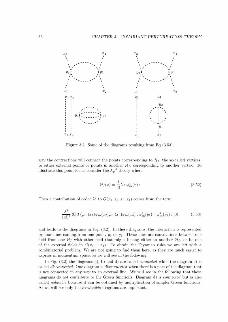
86 CHAPTER 3. COVARIANT PERTURBATION THEORY
x1 x1
x1x1
x2x2
x2 x2
x3
x3
x3
x3x4
x4x4
x4
y1
y1
y1
y1
y2
y2
y2
y2
Figure 3.2: Some of the diagrams resulting from Eq (3.53).
way the contractions will connect the points corresponding to HI , the so-called vertices,to either external points or points in another HI , corresponding to another vertex. Toillustrate this point let us consider the λϕ4 theory where,
HI(x) =1
4!λ : ϕ4
in(x) : (3.52)
Then a contribution of order λ2 to G(x1, x2, x3, x4) comes from the term,
λ2
(4!)2〈0|T (ϕin(x1)ϕin(x2)ϕin(x3)ϕin(x4) : ϕ4
in(y1) :: ϕ4in(y2) : |0〉 (3.53)
and leads to the diagrams in Fig. (3.2). In these diagrams, the interaction is representedby four lines coming from one point, y1 or y2. These lines are contractions between onefield from one HI with other field that might belong either to another HI , or be oneof the external fields in G(x1 · · · x4). To obtain the Feynman rules we are left with acombinatorial problem. We are not going to find them here, as they are much easier toexpress in momentum space, as we will see in the following.
In Fig. (3.2) the diagrams a), b) and d) are called connected while the diagram c) iscalled disconnected. One diagram is disconnected when there is a part of the diagram thatis not connected in any way to an external line. We will see in the following that thesediagrams do not contribute to the Green functions. Diagram d) is connected but is alsocalled reducible because it can be obtained by multiplication of simpler Green functions.As we will see only the irreducible diagrams are important.

3.4. VACUUM–VACUUM AMPLITUDES 87
y1y1
y1
y2y2
y2
y3y3 y4y4y5
a) b) c)
Figure 3.3: Some vacuum–vacuum amplitudes in Eq. (3.54).
3.4 Vacuum–Vacuum amplitudes
We have seen in the previous section examples of the numerator of Eq. (3.34). Let usnow look at the denominator, the so-called vacuum-vacuum amplitudes. Continuing withthe example of λϕ4, some of the diagrams contributing for these amplitudes are shown inFig. (3.3). The diagrams associated with the numerator of Eq. (3.34) can be separatedinto connected and disconnected parts. For all diagrams that have as connected part acontribution of order s in the interaction HI , the numerator of G(x1 · · · xn) takes the form,
∞∑
p=0
(−i)pp!
∫d4y1 · · · d4yp 〈0|T (ϕin(x1) · · ·ϕin(xn)HI(y1) · · · HI(ys)) |0〉c
× p!
s!(p− s)!〈0|T (HI(ys+1) · · · HI(yp)) |0〉 (3.54)
where the subscript c indicates that only the connected parts are included. The combina-torial factor
p
s
=
p!
s!(p− s)!(3.55)
is the number of ways in which we can extract s terms HI from a set of p terms. We writethen Eq. (3.54) in the form (r = p− s),
(−i)ss!
∫d4y1 · · · d4ys 〈0|T (ϕin(x1) · · ·ϕin(xn)HI(y1) · · · H(ys)) |0〉c
×∞∑
r=0
(−i)rr!
∫d4z1 · · · d4zr 〈0|T (HI(z1) · · · HI(zr)) |0〉 (3.56)
This equation has the form of a connected diagram of order s times an infinite seriesof vacuum-vacuum amplitudes, that cancels exactly against the denominator. This is truefor all orders, and therefore we can write,
G(x1, · · · xn) =
∑iGi(x1 · · · xn)∑
kDk=
(∑
iGci (x1, · · · xn))(
∑kDk)∑
kDk
88 CHAPTER 3. COVARIANT PERTURBATION THEORY
=∑
i
Gci (x1 · · · xn) (3.57)
where Gci are the connected diagrams and Dk the disconnected ones. This result meansthat we can simply ignore completely the disconnected diagrams and consider only theconnected ones when evaluating the Green functions. These are simply the sum of allconnected diagrams, simplifying enormously the structure of Eq. (3.34).
3.5 Feynman rules for λϕ4
To understand how the Feynman rules appear, let us consider the case of a real scalarfield with an interaction of the form,
HI =λ
4!: ϕ4
in := −LI (3.58)
To be more precise we consider two particles in the initial and final state. Then the Smatrix element is,
Sfi =⟨p′1p′2; out|p1p2; in
⟩
= (i)4∫d4x1d
4x2d4x3d
4x4e−ip1·x1−ip2·x2+ip′ix3+ip′2·x4
(⊔⊓x1 +m2) · · · (⊔⊓x4 +m2) 〈0|T (ϕ(x1)ϕ(x2)ϕ(x3)ϕ(x4)) |0〉 (3.59)
For the Green function we use the expressions in Eqs. (3.34) and (3.57) and we obtain,
G(x1, x2, x3, x4) =
∞∑
p=0
(−iλ)pp!
∫d4z1 · · · d4zp
〈0|T (ϕin(x1)ϕin(x2)ϕin(x3)ϕin(x4) :ϕ4in(z1)
4!: · · · : ϕ
4in(zp)
4!:) |0〉c (3.60)
As the case p = 0 is trivial (there is no interaction) we begin by the p = 1 case.
• p = 1
Then the Green function is,
G(x1, x2, x3, x4) = (−iλ)∫d4z 〈0|T
(ϕin(x1)ϕin(x2)ϕin(x3)ϕin(x4) :
ϕ4in(z)
4!:
)|0〉
= (−iλ)4!4!
∫d4z∆F (x1 − z)∆F (x2 − z)∆F (x3 − z)∆F (x4 − z)
(3.61)
to which corresponds, in the configuration space, the diagram of Fig. (3.4). To proceed,

3.5. FEYNMAN RULES FOR λϕ4 89
x1 x2
x3 x4
z
Figure 3.4: Vertex in the λφ4 theory.
we introduce the Fourier transform of the propagators, that is,
∆F (x1 − z) =
∫d4q1(2π)4
e−iq1·(x1−z)∆F (q1) (3.62)
where
∆F (q1) =i
q21 −m2(3.63)
then
G(x1, · · · x4) = (−iλ)∫d4z
d4q1(2π)4
· · · d4q4
(2π)4e−iq1·x1−iq2x2−iq3x3−iq4x4+i(q1+q2+q3+q4)·z
∆F (q1)∆F (q2)∆F (q3)∆F (q4)
= (−iλ)∫
d4q1(2π)4
· · · d4q4
(2π)4e−iq1·x1−iq2·x2−iq3·x3−iq4·x4
(2π)4δ4(q1 + q2 + q3 + q4)∆F (q1)∆F (q2)∆F (q3)∆F (q4)
(3.64)
If we now introduce the T matrix transition amplitude, defined by
Sfi = δfi − i(2π)4δ(Pf − Pi) Tfi (3.65)
we obtain
−iTfi = (−iλ) (3.66)
for this amplitude we draw the Feynman diagram of Fig. (3.5), and we associate to thevertex the number (−iλ).
• p = 2
Let us consider now a more complicated case, the evaluation of G(x1 · · · x4) in secondorder in the coupling λ. After this exercise we will be in position to be able to state the

90 CHAPTER 3. COVARIANT PERTURBATION THEORY
p1 p2
p′1 p′2
−i λ
Figure 3.5: Vertex in momentum space.
Feynman rules in momentum space with all generality. From Eq. (3.60) we get in secondorder in λ,
G(x1, · · · x4) =
=(−iλ)2
2!
∫d4z1d
4z2 〈0|T(ϕin(x1)ϕin(x2)ϕin(x3)ϕin(x4) :
ϕ4in(z1)
4!::ϕ4in(z2)
4!:
)|0〉c
=(−iλ)2
2!
∫d4z1d
4z2
(4× 3
4!
)×(4× 3
4!
)× 2
∆F (x1 − z1)∆F (x2 − z1)∆F (z1 − z2)∆F (z1 − z2)∆F (z2 − x3)∆F (z2 − x4)
+∆F (x1 − z1)∆F (x2 − z2)∆F (z1 − z2)∆F (z1 − z2)∆F (z1 − x3)∆F (z2 − x4)
+∆F (x1 − z1)∆F (x2 − z2)∆F (z1 − z2)∆F (z1 − z2)∆F (z1 − x4)∆F (z2 − x3)
+∆F (x1 − z2)∆F (x2 − z2)∆F (z2 − z1)∆F (z2 − z1)∆F (z1 − x3)∆F (z1 − x4)
+∆F (x1 − z2)∆F (x2 − z1)∆F (z1 − z2)∆F (z2 − z1)∆F (z1 − x3)∆F (z2 − x4)
+ ∆F (x1 − z2)∆F (x2 − z1)∆F (z1 − z2)∆F (z1 − z2)∆F (z1 − x4)∆F (z1 − x3)
=(−iλ)2
2!
∫d4z1d
4z2

3.5. FEYNMAN RULES FOR λϕ4 91
x1 x1x1 x2 x2x2
x3 x3x4 x4 x4x3
z1 z1z2 z2z2z11
21
2
1
2__ __ __
+ (z1 ↔ z2)
(3.67)
Let us now go into momentum space, by introducing the Fourier transform of thepropagators. We start by diagram a),
G(a)(x1, x2, x3, x4) =
=(−iλ)2
2!
1
2
∫d4z1d
4z2∆F (x1 − z1)∆F (x2 − z1)∆F (z1 − z2)∆F (z1 − z2)
∆F (z2 − x3)∆F (z2 − x4)
=(−iλ)2
2!
1
2
∫d4z1d
4z2d4q1(2π)4
d4q2(2π)4
d4q3(2π)4
d4q4(2π)4
d4q5(2π)4
d4q6(2π)4
ei[(q1·x1+q2·x2−q3·x3−q4·x4)+z1·(q5−q1−q2+q6)+z2·(q3+q4−q5−q6)]
∆F (q1)∆F (q2)∆F (q3)∆F (q4)∆F (q5)∆F (q6)
=(−iλ)2
2!
1
2(2π)4
∫d4q1(2π)4
· · · d4q5
(2π)4δ4(q1 + q2 − q3 − q4) e
i[q1·x1+q2·x2−q2·x3−q4·x4]
∆F (q1)∆F (q2)∆F (q3)∆F (q4)∆F (q5)∆F (q1 + q2 − q5) (3.68)
Now we insert the last equation into the reduction formula. We get
S(a)fi = (i)4
∫d4x1 · · · d4x4e−i[p1·x1+p2·x2−p
′1·x3−p′2·x4]
(⊔⊓x1 +m2) · · · (⊔⊓x4 +m2)G(a)(x1, · · · , x4) (3.69)
The only dependence of G(a) in the coordinates, xi(i = 1, · · · 4), is in the exponential,therefore,
(⊔⊓xi +m2) → (−q2i +m2) (3.70)
and using(−q2i +m2)∆F (qi) = −i (3.71)
we get
S(a)fi =
(−iλ)22!
1
2
∫d4x1 · · · d4x4
∫d4q1(2π)4
· · · d4q5
(2π)4(2π)4δ4(q1 + q2 − q3 − q4)

92 CHAPTER 3. COVARIANT PERTURBATION THEORY
p1 p2
p′1 p′2
q q − p1 − p212
Figure 3.6:
e−i[x1·(p1−q1)+x2·(p2−q2)−x3·(p′1−q3)−x4·(p′2−q4)]∆F (q5)∆F (q1 + q2 − q5)
=(−iλ)2
2!
1
2
∫d4q1(2π)4
· · · d4q5
(2π)4(2π)4δ4(q1 + q2 − q3 − q4)(2π)
4δ4(p1 − q1)
(2π)4δ4(p2 − q2)(2π)4δ4(p′1 − q3)(2π)
4δ4(p′2 − q4)∆F (q5)∆F (q1 + q2 − q5)
=(−iλ)2
2!
1
2
∫d4q5(2π)4
(2π)4δ4(p1 + p2 − p′1 − p′2)∆F (q5)∆F (p1 + p2 − q5) (3.72)
This expression can be written in the form
S(a)fi = (2π)4δ4(p1 + p2 − p′1 − p′2)
(−iλ)22!
1
2
∫d4q
(2π)4∆F (q)∆F (p1 + p2 − q) (3.73)
If we denote by a′) the diagram a) with the interchange z1 ↔ z2 and redo the calculationwe get exactly the same result as in Eq. (3.73). Therefore,
S(a+a′)fi = (2π)4δ4(p1 + p2 − p′1 − p′2)(−iλ)2
1
2
∫d4q
(2π)4∆F (q)∆F (p1 + p2 − q) (3.74)
or in terms of the Tfi matrix,
−iT (a+a′)fi = (−iλ)2 1
2
∫d4q
(2π)4∆F (q)∆F (p1 + p2 − q) (3.75)
To encode this result we draw the Feynman diagram of Fig. (3.6), that has the sametopology as a) and a′) but in momentum space. We find that in order to evaluate the −iTmatrix, we associate to each vertex a factor (−iλ), to each internal line a propagator ∆F
and for each loop the integral∫ d4q
(2π)4. Besides that we have 4-momentum conservation at
each vertex. Finally there is a symmetry factor (see below) which takes the value 12 for
this diagram.
If we repeat the calculations for diagrams b) + b′) and c) + c′) it is easy to see that weget,
−iT (b+b′)fi = (−iλ)2 1
2
∫d4q
(2π)4∆F (q)∆F (q − p1 + p′1) (3.76)

3.6. FEYNMAN RULES FOR QED 93
p1p1 p2p2
p′1p′1
p′2p′2
q−p1+p′2
q−p1+p′112
12
Figure 3.7:
and
−iT (c+c′)fi = (−iλ)2 1
2
∫d4q
(2π)4∆F (q)∆F (q − p1 + p′2) (3.77)
to which correspond the diagrams of Fig. (3.7).
After this exercise we are in position to state the Feynman rules with all generality forthe λϕ4 theory. These are rules for the −iT matrix, that is, after we factorize (2π)4δ4(· · · ).These are (for a process with n external legs):
1. Draw all topologically distinct diagrams with n external legs.
2. At each vertex multiply by the factor (−iλ).
3. To each internal line associate a propagator ∆F (q).
4. For each loop include an integral∫ d4q
(2π)4 . The direction of this momentum is irrele-
vant, but we have to respect 4-momentum conservation ate each vertex.
5. Multiply by the symmetry factor of the diagram. This is defined by,
S =# of distinct ways of connecting the vertices to the external legs
Permutations of each vertex × Permutations of equal vertices(3.78)
6. Add the contributions of all the topologically distinct diagrams. The result is the−iT matrix amplitude that enters the formula for the cross section.
3.6 Feynman rules for QED
We now turn to the case of QED. Like λφ4, it is a theory without derivatives and therefore,
LI = −HI = −e QψinγµψinAinµ (3.79)
where e is the absolute value of the electron charge, or the proton charge. For the electronthe sign enters explicitly in Q = −1. This way of writing in Eq. (3.79), allows for obvious

94 CHAPTER 3. COVARIANT PERTURBATION THEORY
p p′
k k′
γγ
e−e−
Figure 3.8: Kinematics for the Compton scattering.
generalizations for particles with other charges, like for instance the quarks. For QED wehave then,
LQEDI = e ψinγµψinA
inµ (3.80)
Due to the electric charge conservation, the Green functions that we have to deal withhave an equal number of ψ and ψ fields. In general we have,
G(x1 · · · xnxn+1 · · · x2n; y1 · · · yp) =
= 〈0|T (ψ(x1) · · ·ψ(xn)ψ(xn+1) · · ·ψ(x2n)Aµ1(y1) · · ·Aµp(yp)) |0〉 (3.81)
where, for simplicity, we omit the spinorial indices in the fermion fields. This equation iswritten in terms of the physical fields. Following a similar procedure to the scalar fieldcase, we can obtain an expression for G in terms of the in fields. This will be,
G(x1 · · · x2n; y1 · · · yp) =〈0|Tψin(x1) · · ·ψin(x2n)Aµ1in (y1) · · ·A
µpin (yp) e
[i∫
d4zLI(z)] |0〉〈0|T exp[i
∫d4zLI(z)] |0〉
= 〈0|Tψin(x1) · · ·ψin(x2n)Aµ1in (y1) · · ·Aµpin (yp) e
[i∫
d4tLI(z)] |0〉c(3.82)
where the fields in LI are normal ordered, and 〈0| · · · |0〉c means that we only consider theconnected diagrams. To get the Feynman rules we will evaluate a few simple processes.
3.6.1 Compton scattering
Compton scattering corresponds to the following process,
e− + γ → e− + γ (3.83)
and we choose the kinematics in Fig. (3.8). The S matrix element to evaluate is therefore,
Sfi =⟨(p′, s′), k′; out|(p, s), k; in
⟩(3.84)

3.6. FEYNMAN RULES FOR QED 95
Using the LSZ reduction formula Eq. (2.101), and Eq. (2.109) we can write,
Sfi =
∫d4xd4x′
∫d4yd4y′e−i[p·x+k·y−p
′·x′−k′·y′]εµ(k)ε∗µ′
(k′)
u(p′, s′)α′(i∂→/x′−m)α′β′~⊔⊓y~⊔⊓y′ 〈0|T (ψβ′(x′)ψβ(x)Aµ(y)Aµ′(y
′)) |0〉 (−i∂←/x−m)βαuα(p, s)
(3.85)
Our task is therefore to evaluate the Green function
G(x′, x, y, y′) ≡ 〈0|T (ψβ′(x′)ψβ(x)Aµ(y)Aµ′(y′)) |0〉 (3.86)
If we use Eq. (3.82) and the fact that the interaction has an odd number of fields, we findthat the lowest contribution is quadratic in the interaction2. We get
G(x, x′, y, y′) =
=(ie)2
2!
∫d4z1d
4z2 〈0|T (ψinβ′ (x′)ψinβ (x)Ainµ (y)Ainµ′ (y
′)
: ψin(z1)γσψin(z1)A
inσ (z1) :: ψ
in(z2)γ
ρψin(z2)Ainρ (z2) :) |0〉
=(ie)2
2!(γσ)γδ (γρ)γ′δ′
∫d4z1d
4z2 〈0|T (ψinβ′ (x′)ψinβ (x)Ainµ (y)Ainµ′ (y
′)
: ψinγ (z1)ψ
inδ (z1)A
inσ (z1) :: ψ
inγ′ (z2)ψ
inδ′ (z2)A
inρ (z2) :) |0〉 (3.87)
Now we use Wick’s theorem to write 〈0|T (· · · ) |0〉 in terms of the propagators. We get,
〈0|T (ψinβ′ (x′)ψinβ (x)Ainµ (y)Ainµ′ (y
′) :ψinγ (z1)ψ
inδ (z1)A
inσ (z1) ::ψ
inγ′ (z2)ψ
inδ′ (z2)A
inρ (z2)) :) |0〉
= 〈0|Tψinβ′ (x′)ψinγ (z1) |0〉 〈0|Tψinδ′ (z2)ψ
inβ (x) |0〉 〈0|Tψinδ (z1)ψγ′(z2) |0〉
〈0|T (Ainµ (y)Ainσ (z1)) |0〉 〈0|TAinµ′(y′)Ainρ (z2) |0〉
+ 〈0|Tψinβ′ (x′)ψinγ (z1) |0〉 〈0|Tψinδ′ (z2)ψ
inβ (x) |0〉 〈0|Tψinδ (z1)ψγ′(z2)|0
〈0|TAinµ (y)Ainρ (z2) |0〉 〈0|TAinµ′ (y′)Ainσ (z1) |0〉
+ 〈0|Tψinβ′ (x′)ψinγ′ (z2) |0〉 〈0|Tψinδ (z1)ψ
inβ (x) |0〉 〈0|Tψinδ′ (z2)ψ
inγ (z1) |0〉
〈0|TAinµ (y)Ainσ (z1) |0〉 〈0|TAinµ′ (y′)Ainρ (z2) |0〉
+ 〈0|Tψinβ′ (x′)ψinγ′ (z2) |0〉 〈0|Tψinδ (z1)ψ
inβ (x) |0〉 〈0|Tψinδ′ (z2)ψ
inγ (z1) |0〉
〈0|TAinµ (y)Ainρ (z2) |0〉 〈0|TAinµ′ (y′)Ainσ (z1) |0〉
= SFβ′γ(x′ − z1)SFδ′β(z2 − x)SFδγ′(z1 − z2)DFµσ(y − z1)DFµ′ρ(y
′ − z2)
2By Wick’s theorem the expectation value of an odd number of fields vanishes.

96 CHAPTER 3. COVARIANT PERTURBATION THEORY
xx
xx
x′ x′
x′x′
y
yy
y
y′
y′
y′
y′
z1z1
z1z1
z2z2
z2z2a) b)
c) d)
Figure 3.9: Diagrams for Compton scattering in configuration space.
+SFβ′γ(x′ − z1)SFδ′β(z2 − x)SFδγ′(z1 − z2)DFµρ(y − z2)DFµ′σ(y
′ − z1)
+SFβ′γ′(x′ − z2)SFδβ(z1 − x)SFδ′γ(z2 − z1)DFµσ(y − z1)DFµ′ρ(y
′ − z2)
+SFβ′γ′(x′ − z2)SFδβ(z1 − x)SFδ′γ(z2 − z1)DFµρ(y − z2)DFµ′σ(y
′ − z1) (3.88)
To better understand Eq. (3.88) it is useful to draw the corresponding diagrams inconfiguration space. We show them in Fig. (3.9). From this figure it is clear that b) ≡ c)and a) ≡ d) because z1 and z2 are irrelevant labels. From this we get a factor of 2 thatis going to cancel the 1
2! in Eq. (3.87)3. We have then only two distinct diagrams that wetake as c) and d). Then, including already the factor of 2, we get for diagrama c)
G(c)(x, x′, y, y′) = (ie)2(γσ)γδ(γρ)γ′δ′
∫d4z1d
4z2 SFβ′γ′(x′ − z2)SFδβ(z1 − x)
SFδ′γ(z2 − z1)DFµσ(y − z1)DFµ′ρ(y′ − z2) (3.89)
To proceed we could, like in the case of λϕ4, introduce the Fourier transform of thepropagators. However, it is easier to get rid of the external legs using the results,
(i∂/x −m)αλSFλβ(x− y) = iδαβδ4(x− y)
SFαλ(x− y)(−i∂←/y −m)λβ = iδαβδ
4(x− y) (3.90)
and⊔⊓xDFµν(x− y) = igµνδ
4(x− y) (3.91)
3In fact this result is general, for n vertices we have n! that cancels against the factor 1n!
from theexpansion of the exponential.

3.6. FEYNMAN RULES FOR QED 97
p p′
k k′
µ ν
a) p p′
k k′
µ ν
b)
Figure 3.10: Diagrams for Compton scattering.
We get therefore,
S(c)fi = (ie)2
∫d4xd4x′d4yd4y′e−i(p·x+k·y−p
′·x′−k′·y′)εµ(k)gµσε∗µ′(k′)gµ′ρ
(γσ)γδ(γρ)γ′δ′ u(p
′, s′)α′δα′γ′uα(p, s) δδα∫d4z1d
4z2δ4(x′ − z2)δ
4(x− z1)δ4(y − z1)δ
4(y′ − z2) SFδ′γ(z2 − z1)
= (ie)2∫d4z1d
4z2e−i(p·z1+k·z1−p′·z2−k′·z2)εµ(k)ε∗µ
′
(k′)
u(p′, s′)α′(γµ′)α′δ′SFδ′γ(z2 − z1)(γµ)γαuα(p, s) (3.92)
Finally we use
SF (z2 − z1) =
∫d4q
(2π)4i(q/+m)
q2 −m2 + iǫe−iq·(z2−z1)
≡∫
d4q
(2π)4SF (q)e
−iq·(z2−z1) (3.93)
to get
S(c)fi =
∫d4q
(2π)4d4z1d
4z2e−iz1·(p+k−q)+iz2·(p′+k′−q)
εµ(k)εµ′∗(k′)u(p′, s′)(ieγµ′ )SF (q)(ieγµ)u(p, s)
= (2π)4δ(4)(p+ k − p′ − k)·
εµ(k)εµ′∗(k′)u(p′, s′)(ieγµ′ )SF (p+ k)(ieγµ)u(p, s) (3.94)
Therefore, the T matrix transition amplitude is,
−iT (c)fi = εµ(k)εµ
′∗(k′)u(p′, s′)(ieγµ′)SF (p+ k)(ieγµ)u(p, s) (3.95)
corresponding to the diagram on the left panel of Fig. (3.10). In Eq. (3.95) we factor outthe quantity (ieγµ), because it will be clear that this quantity will be the Feynman rule forthe vertex. The arrows in these diagrams correspond to the flow of electric charge. Noticethat to an electron in the initial state we associate a spinor u(p, s) and for an electron in
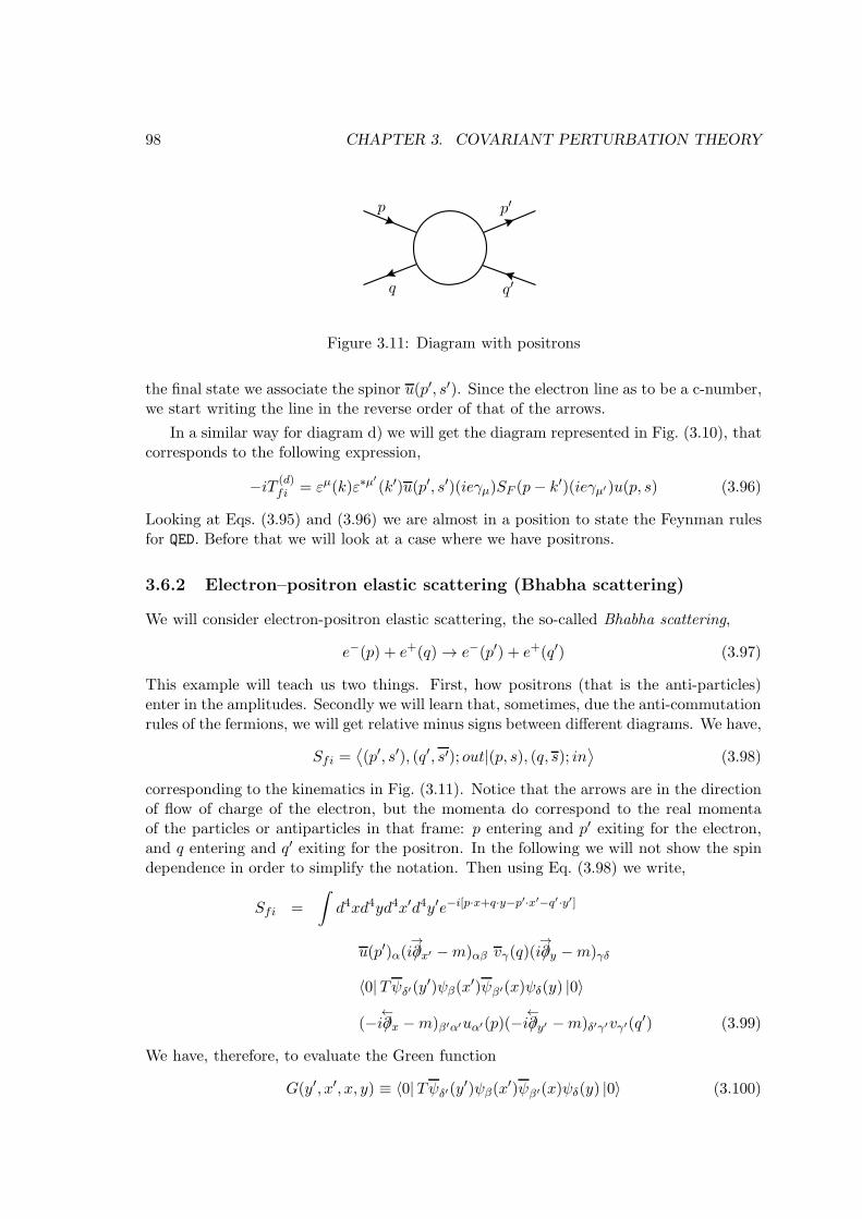
98 CHAPTER 3. COVARIANT PERTURBATION THEORY
p p′
q q′
Figure 3.11: Diagram with positrons
the final state we associate the spinor u(p′, s′). Since the electron line as to be a c-number,we start writing the line in the reverse order of that of the arrows.
In a similar way for diagram d) we will get the diagram represented in Fig. (3.10), thatcorresponds to the following expression,
−iT (d)fi = εµ(k)ε∗µ
′
(k′)u(p′, s′)(ieγµ)SF (p− k′)(ieγµ′)u(p, s) (3.96)
Looking at Eqs. (3.95) and (3.96) we are almost in a position to state the Feynman rulesfor QED. Before that we will look at a case where we have positrons.
3.6.2 Electron–positron elastic scattering (Bhabha scattering)
We will consider electron-positron elastic scattering, the so-called Bhabha scattering,
e−(p) + e+(q) → e−(p′) + e+(q′) (3.97)
This example will teach us two things. First, how positrons (that is the anti-particles)enter in the amplitudes. Secondly we will learn that, sometimes, due the anti-commutationrules of the fermions, we will get relative minus signs between different diagrams. We have,
Sfi =⟨(p′, s′), (q′, s′); out|(p, s), (q, s); in
⟩(3.98)
corresponding to the kinematics in Fig. (3.11). Notice that the arrows are in the directionof flow of charge of the electron, but the momenta do correspond to the real momentaof the particles or antiparticles in that frame: p entering and p′ exiting for the electron,and q entering and q′ exiting for the positron. In the following we will not show the spindependence in order to simplify the notation. Then using Eq. (3.98) we write,
Sfi =
∫d4xd4yd4x′d4y′e−i[p·x+q·y−p
′·x′−q′·y′]
u(p′)α(i∂→/x′ −m)αβ vγ(q)(i∂
→/y −m)γδ
〈0|Tψδ′(y′)ψβ(x′)ψβ′(x)ψδ(y) |0〉
(−i∂←/x −m)β′α′uα′(p)(−i∂
←/y′ −m)δ′γ′vγ′(q
′) (3.99)
We have, therefore, to evaluate the Green function
G(y′, x′, x, y) ≡ 〈0|Tψδ′(y′)ψβ(x′)ψβ′(x)ψδ(y) |0〉 (3.100)
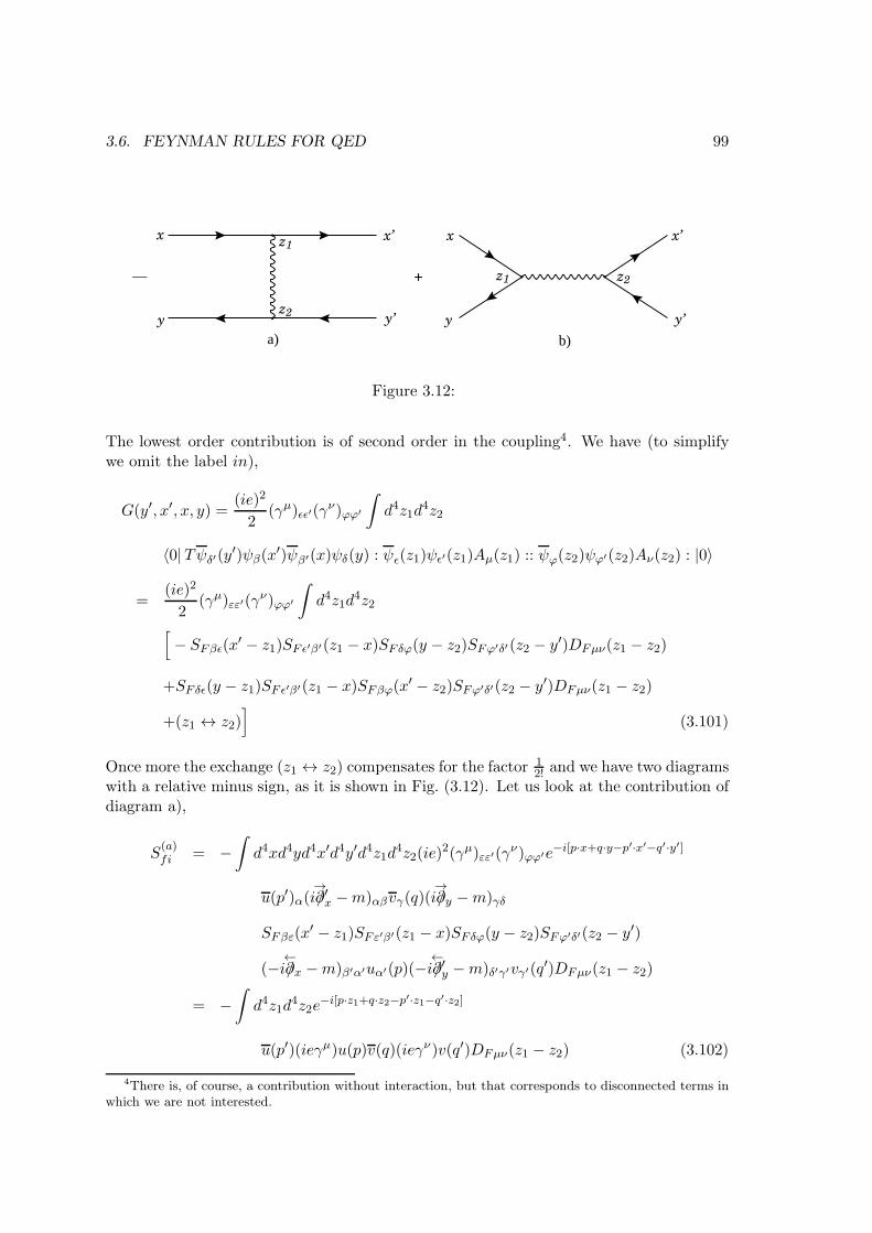
3.6. FEYNMAN RULES FOR QED 99
+
b)a)
x x
y y
z1 z2
z1
z2
x’
y’
x’
y’
__
Figure 3.12:
The lowest order contribution is of second order in the coupling4. We have (to simplifywe omit the label in),
G(y′, x′, x, y) =(ie)2
2(γµ)ǫǫ′(γ
ν)ϕϕ′
∫d4z1d
4z2
〈0|Tψδ′(y′)ψβ(x′)ψβ′(x)ψδ(y) : ψǫ(z1)ψǫ′(z1)Aµ(z1) :: ψϕ(z2)ψϕ′(z2)Aν(z2) : |0〉
=(ie)2
2(γµ)εε′(γ
ν)ϕϕ′
∫d4z1d
4z2
[− SFβǫ(x
′ − z1)SFǫ′β′(z1 − x)SFδϕ(y − z2)SFϕ′δ′(z2 − y′)DFµν(z1 − z2)
+SFδǫ(y − z1)SFǫ′β′(z1 − x)SFβϕ(x′ − z2)SFϕ′δ′(z2 − y′)DFµν(z1 − z2)
+(z1 ↔ z2)]
(3.101)
Once more the exchange (z1 ↔ z2) compensates for the factor 12! and we have two diagrams
with a relative minus sign, as it is shown in Fig. (3.12). Let us look at the contribution ofdiagram a),
S(a)fi = −
∫d4xd4yd4x′d4y′d4z1d
4z2(ie)2(γµ)εε′(γ
ν)ϕϕ′e−i[p·x+q·y−p′·x′−q′·y′]
u(p′)α(i∂→/′x −m)αβvγ(q)(i∂
→/y −m)γδ
SFβε(x′ − z1)SFε′β′(z1 − x)SFδϕ(y − z2)SFϕ′δ′(z2 − y′)
(−i∂←/x −m)β′α′uα′(p)(−i∂
←/′y −m)δ′γ′vγ′(q
′)DFµν(z1 − z2)
= −∫d4z1d
4z2e−i[p·z1+q·z2−p′·z1−q′·z2]
u(p′)(ieγµ)u(p)v(q)(ieγν)v(q′)DFµν(z1 − z2) (3.102)
4There is, of course, a contribution without interaction, but that corresponds to disconnected terms inwhich we are not interested.
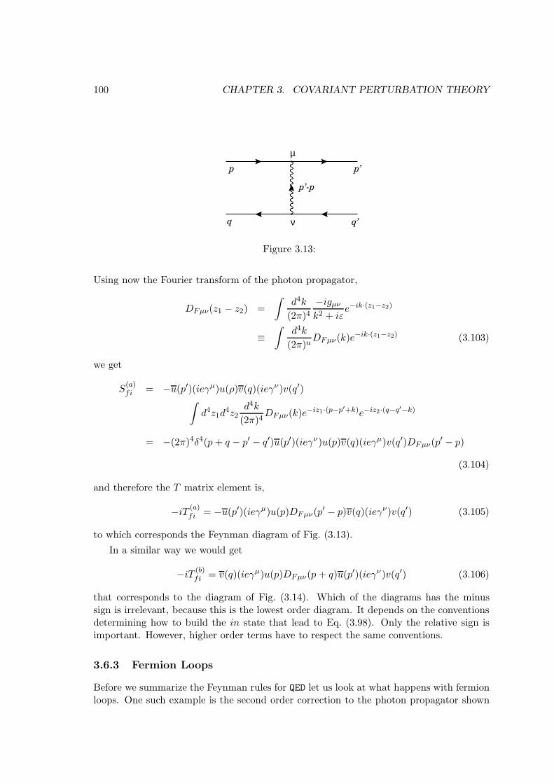
100 CHAPTER 3. COVARIANT PERTURBATION THEORY
p p’
q q’
p’-p
µ
ν
Figure 3.13:
Using now the Fourier transform of the photon propagator,
DFµν(z1 − z2) =
∫d4k
(2π)4−igµνk2 + iε
e−ik·(z1−z2)
≡∫
d4k
(2π)uDFµν(k)e
−ik·(z1−z2) (3.103)
we get
S(a)fi = −u(p′)(ieγµ)u(ρ)v(q)(ieγν)v(q′)
∫d4z1d
4z2d4k
(2π)4DFµν(k)e
−iz1·(p−p′+k)e−iz2·(q−q′−k)
= −(2π)4δ4(p + q − p′ − q′)u(p′)(ieγν)u(p)v(q)(ieγµ)v(q′)DFµν(p′ − p)
(3.104)
and therefore the T matrix element is,
−iT (a)fi = −u(p′)(ieγµ)u(p)DFµν(p
′ − p)v(q)(ieγν)v(q′) (3.105)
to which corresponds the Feynman diagram of Fig. (3.13).
In a similar way we would get
−iT (b)fi = v(q)(ieγµ)u(p)DFµν(p + q)u(p′)(ieγν)v(q′) (3.106)
that corresponds to the diagram of Fig. (3.14). Which of the diagrams has the minussign is irrelevant, because this is the lowest order diagram. It depends on the conventionsdetermining how to build the in state that lead to Eq. (3.98). Only the relative sign isimportant. However, higher order terms have to respect the same conventions.
3.6.3 Fermion Loops
Before we summarize the Feynman rules for QED let us look at what happens with fermionloops. One such example is the second order correction to the photon propagator shown

3.6. FEYNMAN RULES FOR QED 101
p
q q’
p’
µ νp+q
Figure 3.14:
Figure 3.15: Vacuum polarization
in Fig. (3.15). First of all, the loop orientation it is only relevant if leads to topologicallydifferent diagrams. Therefore the diagrams of Fig. (3.16) are topologically equivalent andonly one should be considered. However the diagrams in Fig. (3.17) are topologicallydistinct and both should be considered.
Figure 3.16: Topologically equivalent diagrams
The second aspect that is relevant is a possible sign coming from the anti-commutationof the fermion fields, that should affect some diagrams, and in particular the fermion loop.To understand this sign we should note that by definition of loop, the internal lines arenot connected to external fermion lines, they should originate only in the interaction.Therefore they should come from terms of the form
〈0|T · · · : ψ(z1)A/(z1)ψ(z1) : · · · : ψ(zn)A/(zn)ψ(zn) : · · · |0〉 . (3.107)
Now it is clear that in order to make the appropriate contractions of the fermion fieldsto bring them to the form of the Feynman propagator, 〈0|Tψ(z1)ψ(z2) |0〉, it is necessary

102 CHAPTER 3. COVARIANT PERTURBATION THEORY
11
22 33
44
Figure 3.17: Topologically distinct diagrams
to make an odd number of permutations of the fermion fields, and therefore we get a (−)sign for the loops. This sign is physically relevant because there is a lowest order diagramwhere the photons do not interact, corersponding to the free propagator. So the minussign is defined in relation to this lowest order diagram and therefore it is not arbitrary(see the difference with respect to the discussion of the Bahbha scattering).
3.6.4 Feynman rules for QED
We are now in position to state the Feynman rules for QED
1. For a given process, draw all topologically distinct diagrams.
2. For each electron entering a diagram a factor u(p, s). If it leaves the diagram a factoru(p, s).
3. For each positron leaving the diagram (final state) a factor v(p, s). It it enters thediagram (initial state) then we have a factor v(p, s).
4. For each photon in the initial state we have the vector εµ(k) and in the final stateε∗µ(k).
5. For each internal fermionic line the propagator
SFαβ(p) = i(p/+m)αβp2 −m2 + iε
(3.108)p αβ
6. For each virtual photon the propagator (Feynman gauge)
DFµν(k) = −igµνk2
(3.109)µ νk
7. For each vertex the factor

3.7. GENERAL FORMALISM FOR GETTING THE FEYNMAN RULES 103
ieγµ (3.110)µ
α
β
8. For each internal momentum, not fixed by conservation of momenta, as in the caseof loops, a factor
∫d4q
(2π)4(3.111)
9. For each loop of fermions a −1 sign.
10. A factor of −1 between diagrams that differ by exchange of fermionic lines. In doubt,revert to Wick’s theorem.
Comments
• In QED there are no symmetry factors, that is, they are always equal to 1.
• In our discussion we did not consider the Z factors that come in the reductionformulas, like in Eq. (2.65). This is true in lowest order in perturbation theory.They can be calculated also in perturbation theory. Their definition is (for instancefor the electron),
limp/→m
S′F (p) = Z2SF (p) (3.112)
where S′F (p) is the propagator of the theory with interactions. Then we can obtain,in perturbation theory,
Z2 = 1 +O(α) + · · · (3.113)
In higher orders it is necessary to correct the external lines with these√Z factors.
3.7 General formalism for getting the Feynman rules
After showing how to obtain the Feynman rules for λφ4 and QED, we are going to presenthere, without proof, a general method to obtain the Feynman rules of any theory, includingthe case when the interactions have derivatives, that we have excluded up to now, andthat is very important for the Standard Model. This method can only be fully justifiedwith the methods of Chapter 5. For simplicity we will consider only scalar fields.
The starting point is the action taken as a functional of the fields,
Γ0[ϕ] ≡∫d4xL[ϕ]· (3.114)

104 CHAPTER 3. COVARIANT PERTURBATION THEORY
In fact, Γ0[ϕ] is the generating functional of the one particle irreducible Green functionsin lowest order, as we will see in Chapter 5. The rules are as follows:
Propagators
1. Start by evaluating Γ(2)0 (xi, xj) ≡
δ2Γ0[ϕ]
δϕ(xi)δϕ(xj)
2. Then evaluate the Fourier Transform (FT) to get Γ(2)0 (pi, pj) defined by the relation
(2π)4δ4(pi + pj)Γ(2)0 (pi, pj) ≡
∫d4xid
4xje−i(pi·xi+pj ·xj)Γ(2)
0 (xi, xj) (3.115)
where all the momenta are incoming.
3. The Feynman propagator is then
G(0)F ij = i[Γ
(2)0 (pi, pj)]
−1 . (3.116)
Do not forget that pi = −pj.
Vertices
1. Evaluate Γ(n)0 (x1 · · · xn) = δnΓ0[ϕ]
δϕ(x1) · · · δϕ(xn)2. Then take the Fourier Transform to obtain
(2π)4δ4(p1 + p2 + · · ·+ pn)Γ(n)0 (p1 · · · pn)
≡∫d4x1 · · · d4xne−i(p1·x1+···pn·xn)Γ(n)
0 (x1 · · · xn) (3.117)
3. The vertex in momenta space is then given by the rule
iΓ(n)0 (p1, · · · pn) (3.118)
Comments

3.7. GENERAL FORMALISM FOR GETTING THE FEYNMAN RULES 105
• For fermionic fields it is necessary to take care with the order of the derivation. Theconvention that we take is
δ2
δψα(x)δψβ(y)
(ψ(z)Γψ(z)
)≡ Γβαδ
4(z − x)δ4(z − y) (3.119)
ψα(x) e ψβ(x) are here taken as classical anti-commuting fields (Grassmann variables,see Chapter 5).
• The functional derivatives are defined by
δϕi(x)
δϕk(y)≡ δikδ
4(x− y) (3.120)
3.7.1 Example: scalar electrodynamics
The Lagrangian is
L = (∂µ − ieQAµ)ϕ∗(∂µ + ieQAµ)ϕ−mϕ∗ϕ+ LMaxwell −
λ
4(ϕ∗ϕ)2 (3.121)
ThereforeLint = −ieQϕ∗∂
↔µϕA
µ + e2Q2ϕ∗ϕAµAµ (3.122)
The propagators are the usual ones, let us consider only the vertices. There are twovertices. The cubic vertex is
µk
p
qϕ
ϕ∗
Figure 3.18: Cubic vertex in scalar QED.
Γ(3)µ (x1, x2, x3) = −ieQ
∫d4zδ4(z − x1)(∂
→µ − ∂
←µ)δ
4(z − x2)δ4(z − x3) (3.123)
therefore
(2π)4δ4(p + k + q)Γ(3)µ (p, q, k) ≡ −ieQ
∫d4zd4x1d
4x2d4x3e
−i(x1·p+x2·q+x3·k)
δ4(z − x1) (∂→µ − ∂
←µ)δ
4(z − x2)δ4(z − x3)

106 CHAPTER 3. COVARIANT PERTURBATION THEORY
= −ieQ∫d4zd4x2e
−i[(p+k)·z+q·x2]∂µδ4(z − x2)
+ieQ
∫d4zd4x1e
−i[p·x1+(q+k)·z]∂µδ4(z − x1)
= −ieQ(ipµ − iqµ)(2π)4δ4(p+ q + k) (3.124)
Therefore we obtain for this vertex
iΓµ(p, q, k) = ieQ (pµ − qµ) = −ieQ (qµ − pµ) (3.125)
The other vertex is
µ ν
k1 k2
p q
Figure 3.19: Quartic vertex in scalar QED (seagull).
We obtain,
Γ(4)µν (x1, x2, x3, x4) = 2e2Q2δ4(x1 − x2)δ
4(x1 − x3)δ4(x1 − x4)gµν (3.126)
and
Γ(4)µν (p, q, k1, k2) = 2(eQ)2gµν (3.127)
and we finally get for the Feynman rule.
i2e2Q2 gµν (3.128)
Comment
• From the above results we can enunciate a simple rule for interactions that havederivatives of fields.
Consider that we have one field in the Lagrangian that has a derivative,say ∂µφ. Then the rule is
∂µφ→ −i (incoming momentum)µ (3.129)
In the end do not forget to multiply the result by i.

3.7. GENERAL FORMALISM FOR GETTING THE FEYNMAN RULES 107
• As an example consider the following term in the Lagrangian for scalar electrody-namics
L = ieQ∂µϕ∗ϕAµ + · · · (3.130)
If p is the incoming momentum of the line associated with the field ϕ∗, see Fig. 3.18,we have
Vertex = i× (ieQ)× (−ipµ) = i eQ pµ (3.131)
in agreement with Eq. (3.125).

108 CHAPTER 3. COVARIANT PERTURBATION THEORY
Problems for Chapter 3
3.1 Show explicitly that Wick’s theorem is valid for the case of 4 fields, that is
T (ϕin(x1)ϕin(x2)ϕin(x3)ϕin(x4)) =: ϕin(x1) · · ·ϕin(x4) : + · · · (3.132)
3.2 For the case of the λϕ4 theory verify the Feynman rules for the diagrams
p1p1 p2p2
p′1p′1
p′2p′2
q−p1+p′2
q−p1+p′112
12
3.3 Consider a theory with the following interaction Lagrangian
LI = − λ
3!ϕ3in (3.133)
• a) Find the Feynman rules for this theory.
• b) Find the symmetry factor for the diagram
3.4 Verify that for Compton scattering the diagram

Problems 109
bp p′
k k′
µ ν
gives the result of Eq. (3.96).
3.5 Verify Eq. (3.106).
3.6 Show that in QED the symmetry factors are always 1.
3.7 Explicitly calculate the T matrix element for the process e+e− → γγ and verify thatis in agreement with the general rules.
3.8 Show that the amplitudes for e+e− → γγ and e−γ → e−γ are related. How can oneobtain one from the other?

110 CHAPTER 3. COVARIANT PERTURBATION THEORY
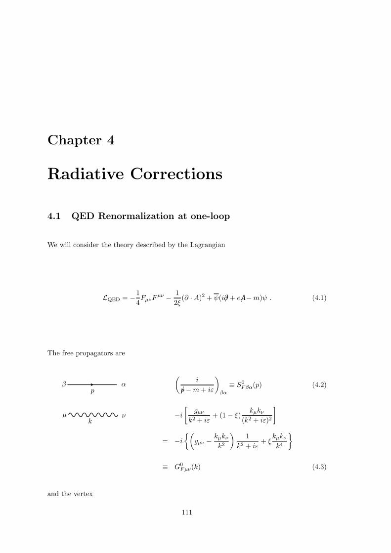
Chapter 4
Radiative Corrections
4.1 QED Renormalization at one-loop
We will consider the theory described by the Lagrangian
LQED = −1
4FµνF
µν − 1
2ξ(∂ ·A)2 + ψ(i∂/+ eA/−m)ψ . (4.1)
The free propagators are
(i
p/−m+ iε
)
βα
≡ S0Fβα(p) (4.2)
−i[
gµνk2 + iε
+ (1− ξ)kµkν
(k2 + iε)2
]
= −i(
gµν −kµkνk2
)1
k2 + iε+ ξ
kµkνk4
≡ G0Fµν(k) (4.3)
αβp
µ νk
and the vertex
111

112 CHAPTER 4. RADIATIVE CORRECTIONS
+ie(γµ)βα e = |e| > 0 (4.4)
e−
e−γ
We will now consider the one-loop corrections to the propagators and to the vertex. Wewill work in the Feynman gauge (ξ = 1).
4.1.1 Vacuum Polarization
In first order the contribution to the photon propagator is given by the diagram of Fig. 4.1that we write in the form
kk
p
p+ k
Figure 4.1: Vacuum polarization.
G(1)µν (k) ≡ G0
µµ′(k) iΠµ′ν′(k)G0
ν′ν(k) (4.5)
where
iΠµν(k) = −(+ie)2∫
d4p
(2π)4Tr[γµ(p/+m)γν(p/+ k/+m)]
(p2 −m2 + iε)((p + k)2 −m2 + iε)(4.6)
= −4e2∫
d4p
(2π)4[2pµpν + pµkν + pνkµ − gµν(p
2 + p · k −m2)
(p2 −m2 + iε)((p + k)2 −m2 + iε)
Simple power counting indicates that this integral is quadratically divergent for largevalues of the internal loop momenta. In fact the divergence is milder, only logarithmic. Theintegral being divergent we have first to regularize it and then to define a renormalizationprocedure to cancel the infinities. For this purpose we will use the method of dimensionalregularization. For a value of d small enough the integral converges. If we define ǫ = 4−d,

4.1. QED RENORMALIZATION AT ONE-LOOP 113
in the end we will have a divergent result in the limit ǫ→ 0. We get therefore1
iΠµν(k, ǫ) = −4e2 µǫ∫
ddp
(2π)d[2pµpν + pµkν + pνkµ − gµν(p
2 + p · k −m2)]
(p2 −m2 + iε)((p + k)2 −m2 + iε)
= −4e2 µǫ∫
ddp
(2π)dNµν(p, k)
(p2 −m2 + iε)((p + k)2 −m2 + iε)(4.7)
where
Nµν(p, k) = 2pµpν + pµkν + pνkµ − gµν(p2 + p · k −m2) (4.8)
To evaluate this integral we first use the Feynman parameterization to rewrite the denom-inator as a single term. For that we use (see Appendix)
1
ab=
∫ 1
0
dx
[ax+ b(1− x)]2(4.9)
to get
iΠµν(k, ǫ) = −4e2 µǫ∫ 1
0dx
∫ddp
(2π)dNµν(p, k)
[x(p+ k)2 − xm2 + (1− x)(p2 −m2) + iε]2
= −4e2 µǫ∫ 1
0dx
∫ddp
(2π)dNµν(p, k)
[p2 + 2k · px+ xk2 −m2 + iε]2
= −4e2 µǫ∫ 1
0dx
∫ddp
(2π)dNµν(p, k)
[(p+ kx)2 + k2x(1− x)−m2 + iε]2(4.10)
For dimension d sufficiently small this integral converges and we can change variables
p→ p− kx (4.11)
We then get
iΠµν(k, ǫ) = −4e2 µǫ∫ 1
0dx
∫ddp
(2π)dNµν(p− kx, k)
[p2 − C + iǫ]2(4.12)
where
C = m2 − k2x(1− x) (4.13)
Nµν is a polynomial of second degree in the loop momenta as can be seen from Eq. (4.8).However as the denominator in Eq. (4.12) only depends on p2 is it easy to show that
∫ddp
(2π)dpµ
[p2 − C + iǫ]2= 0
∫ddp
(2π)dpµpν
[p2 − C + iǫ]2=
1
dgµν
∫ddp
(2π)dp2
[p2 − C + iǫ]2(4.14)
1Where µ is a parameter with dimensions of a mass that is introduced to ensure the correct dimensionsof the coupling constant in dimension d, that is, [e] = 4−d
2= ǫ
2. We take then e → eµ
ǫ2 . For more details
see the Appendix.

114 CHAPTER 4. RADIATIVE CORRECTIONS
x
x
Re p0
Im p0
Figure 4.2: Wick rotation.
This means that we only have to calculate integrals of the form
Ir,m =
∫ddp
(2π)d(p2)r
[p2 − C + iǫ]m
=
∫dd−1p(2π)d
∫dp0
(p2)r
[p2 − C + iǫ]m(4.15)
To make this integration we will use integration in the plane of the complex variable p0 asdescribed in Fig. 4.2. The deformation of the contour corresponds to the so called Wickrotation,
p0 → ip0E ;
∫ +∞
−∞→ i
∫ +∞
−∞dp0E (4.16)
and p2 = (p0)2 − |~p|2 = −(p0E)2 − |~p|2 ≡ −p2E, where pE = (p0E, ~p) is an euclidean vector,
that isp2E = (p0E)
2 + |~p|2 (4.17)
We can then write (see the Appendix for more details),
Ir,m = i(−1)r−m∫
ddpE(2π)d
p2r
E[p2E + C
]m (4.18)
where we do not need the iǫ anymore because the denominator is positive definite2(C > 0).To proceed with the evaluation of Ir,m we write,
∫ddpE =
∫dp p d−1 dΩd−1 (4.19)
where p =√
(p0E)2 + |~p|2 is the length of of vector pE in the euclidean space with d
dimensions and dΩd−1 is the solid angle that generalizes spherical coordinates. We canshow (see Appendix) that ∫
dΩd−1 = 2πd2
Γ(d2)(4.20)
2The case when C < 0 is obtained by analytical continuation of the final result.

4.1. QED RENORMALIZATION AT ONE-LOOP 115
The p integral is done using the result,
∫ ∞
0dx
xp
(x2 + C)m=
Γ(p+12
)C
12(p−2m+1)Γ
(−p
2 +m− 12
)
2Γ(m)(4.21)
and we finally get
Ir,m = iCr−m+ d2(−1)r−m
(4π)d2
Γ(r + d2)
Γ(d2 )
Γ(m− r − d2 )
Γ(m)(4.22)
Note that the integral representation of Ir,m, Eq. (4.15) is only valid for d < 2(m − r) toensure the convergence of the integral when p→ ∞. However the final form of Eq. (4.22)can be analytically continued for all the values of d except for those where the functionΓ(m− r − d/2) has poles, which are (see section C.6),
m− r − d
26= 0,−1,−2, . . . (4.23)
For the application to dimensional regularization it is convenient to write Eq. (4.22) aftermaking the substitution d = 4− ǫ. We get
Ir,m = i(−1)r−m
(4π)2
(4π
C
) ǫ2
C2+r−m Γ(2 + r − ǫ2)
Γ(2− ǫ2)
Γ(m− r − 2 + ǫ2)
Γ(m)(4.24)
that has poles for m− r − 2 ≤ 0 (see section C.6).
We now go back to calculate Πµν . First we notice that after the change of variables ofEq. (4.11) we get, neglecting terms that vanish due to Eq. (4.14),
Nµν(p− kx, k) = 2pµpν + 2x2kµkν − 2xkµkν − gµν(p2 + x2k2 − xk2 −m2
)(4.25)
and therefore
Nµν ≡ µǫ∫
ddp
(2π)dNµν(p − kx, k)
[p2 − C + iǫ]2
=
(2
d− 1
)gµνµ
ǫI1,2 +
[− 2x(1− x)kµkν+x(1− x)k2gµν + gµνm
2
]µǫI0,2 (4.26)
Using now Eq. (4.24) we can write
µǫI0,2 =i
16π2
(4πµ2
C
) ǫ2 Γ( ǫ2)
Γ(2)
=i
16π2
(∆ǫ − ln
C
µ2
)+O(ǫ) (4.27)
where we have used the expansion of the Γ function, Eq. (C.47),
Γ( ǫ2
)=
2
ǫ− γ +O(ǫ) (4.28)

116 CHAPTER 4. RADIATIVE CORRECTIONS
γ being the Euler constant and we have defined, Eq. (C.50),
∆ǫ =2
ǫ− γ + ln 4π (4.29)
In a similar way
µǫI1,2 = − i
16π2
(4πµ2
C
) ǫ2
CΓ(3− ǫ
2)
Γ(2− ǫ2)
Γ(−1 + ǫ2)
Γ(2)
=i
16π2C
(1 + 2∆ǫ − 2 ln
C
µ2
)+O(ǫ) (4.30)
Due to the existence of a pole in 1/ǫ in the previous equations we have to expand allquantities up to O(ǫ). This means for instance, that
2
d− 1 =
2
4− ǫ− 1 = −1
2+
1
8ǫ+O(ǫ2) (4.31)
Substituting back into Eq. (4.26), and using Eq. (4.13), we obtain
Nµν = gµν
[−1
2+
1
8ǫ+O(ǫ2)
] [i
16π2C
(1 + 2∆ǫ − 2 ln
C
µ2
)+O(ǫ)
]
+
[− 2x(1− x)kµkν+x(1− x)k2gµν + gµνm
2
] [i
16π2
(∆ǫ − ln
C
µ2
)+O(ǫ)
]
= − i
16π2kµkν
[(∆ǫ − ln
C
µ2
)2x(1 − x)
]
+i
16π2gµνk
2
[∆ǫ
(x(1− x) + x(1− x)
)+ ln
C
µ2
(− x(1− x)− x(1− x)
)
+ x(1− x)
(1
2− 1
2
)]
+i
16π2gµνm
2
[∆ǫ(−1 + 1) + ln
C
µ2(1− 1) + (−1
2+
1
2)
](4.32)
and finally
Nµν =i
16π2
(∆ǫ − ln
C
µ2
)(gµνk
2 − kµkν)2x(1− x) (4.33)
Now using Eq. (4.7) we get
Πµν(k) = −4e21
16π2(gµνk
2 − kµkν) ∫ 1
0dx 2x(1− x)
(∆ǫ − ln
C
µ2
)
= −(gµνk
2 − kµkν)Π(k2, ǫ) (4.34)
where
Π(k2, ǫ) ≡ 2α
π
∫ 1
0dx x(1− x)
[∆ǫ − ln
m2 − x(1− x)k2
µ2
](4.35)

4.1. QED RENORMALIZATION AT ONE-LOOP 117
+ +
+ + . . .
=
=Gµν
Figure 4.3: Full photon propagator.
This expression clearly diverges as ǫ → 0. Before we show how to renormalize itlet us discuss the meaning of Πµν(k). The full photon propagator is given by the seriesrepresented in Fig. 4.3, where
≡ iΠµν(k) = sum of all one-particle irreducible(proper) diagrams to all orders
(4.36)
In lowest order we have the contribution represented in Fig. 4.4, which is what we have
=
Figure 4.4: Lowest order contribution.
just calculated. To continue it is convenient to rewrite the free propagator of the photon(in an arbitrary gauge ξ) in the following form
iG0µν =
(gµν −
kµkνk2
)1
k2+ ξ
kµkνk4
= P Tµν1
k2+ ξ
kµkνk4
≡ iG0Tµν + iG0L
µν (4.37)
where we have introduced the transversal projector P Tµν defined by
P Tµν =
(gµν −
kµkνk2
)(4.38)

118 CHAPTER 4. RADIATIVE CORRECTIONS
obviously satisfying the relations,
kµP Tµν = 0
P TµνP Tνρ = P Tµρ
(4.39)
The full photon propagator can also in general be written separating its transversal anlongitudinal parts
Gµν = GTµν +GLµν (4.40)
where GTµν satisfies
GTµν = P TµνGµν (4.41)
Eq. (4.34) means that, to first order, the vacuum polarization tensor is transversal,that is
iΠµν(k) = −ik2P Tµν Π(k) (4.42)
This result is in fact valid to all orders of perturbation theory, a result that can be shownusing the Ward-Takahashi identities. This means that the longitudinal part of the photonpropagator is not renormalized,
GLµν = G0Lµν (4.43)
For the transversal part we obtain from Fig. 4.3,
iGTµν = P Tµν1
k2+ P Tµµ′
1
k2(−i)k2P Tµ′ν′Π(k2)(−i)P Tν′ν
1
k2
+P Tµρ1
k2(−i)k2P Tρλ Π(k2)(−i)P Tλτ
1
k2(−i)k2P Tτσ Π(k2)(−i)P Tσν
1
k2+ · · ·
= P Tµν1
k2[1−Π(k2) + Π2(k2) + · · ·
](4.44)
which gives, after summing the geometric series,
iGTµν = P Tµν1
k2[1 + Π(k2)
] (4.45)
All that we have done up to this point is formal because the function Π(k) diverges.The most satisfying way to solve this problem is the following. The initial lagrangianfrom which we started has been obtained from the classical theory and nothing tell usthat it should be exactly the same in quantum theory. In fact, as we have just seen, thenormalization of the wave functions is changed when we calculate one-loop corrections,and the same happens to the physical parameters of the theory, the charge and the mass.Therefore we can think that the correct lagrangian is obtained by adding corrections to the

4.1. QED RENORMALIZATION AT ONE-LOOP 119
classical lagrangian, order by order in perturbation theory, so that we keep the definitionsof charge and mass as well as the normalization of the wave functions. The terms that weadd to the lagrangian are called counterterms3. The total lagrangian is then,
Ltotal = L(e,m, ...) + ∆L (4.46)
Counterterms are defined from the normalization conditions that we impose on the fieldsand other parameters of the theory. In QED we have at our disposal the normalizationof the electron and photon fields and of the two physical parameters, the electric chargeand the electron mass. The normalization conditions are, to a large extent, arbitrary. Itis however convenient to keep the expressions as close as possible to the free field case,that is, without radiative corrections. We define therefore the normalization of the photonfield as,
limk→0
k2iGRTµν = 1 · P Tµν (4.47)
where GRTµν is the renormalized propagator (the transversal part) obtained from the la-grangian Ltotal. The justification for this definition comes from the following argument.Consider the Coulomb scattering to all orders of perturbation theory. We have then thesituation described in Fig. 4.5. Using the Ward-Takahashi identities one can show that
=
++ +
Figure 4.5: Corrections to Coulomb scattering.
the last three diagrams cancel in the limit q = p′ − p → 0. Then the normalization con-dition, Eq. (4.47), means that we have the situation described in Fig. 4.6, that is, theexperimental value of the electric charge is determined in the limit q → 0 of the Coulombscattering.
3This interpretation in terms of quantum corrections makes sense. In fact we can show that an expansionin powers of the coupling constant can be interpreted as an expansion in hL, where L is the number of theloops in the expansion term.

120 CHAPTER 4. RADIATIVE CORRECTIONS
=limq→0
Figure 4.6: Definition of the electric charge.
The counterterm lagrangian has to have the same form as the classical lagrangian torespect the symmetries of the theory. For the photon field it is traditional to write
∆L = −1
4(Z3 − 1)FµνF
µν = −1
4δZ3 FµνF
µν (4.48)
corresponding to the following Feynman rule
µ νkk − i δZ3k
2
(gµν −
kµkνk2
)(4.49)
We have then
iΠµν = iΠloopµν − i δZ3k2
(gµν −
kµkνk2
)
= −i (Π(k, ǫ) + δZ3) k2 P Tµν (4.50)
Therefore we should make the substitution
Π(k, ǫ) → Π(k, ǫ) + δZ3 (4.51)
in the photon propagator. We obtain,
iGTµν = P Tµν1
k21
1 + Π(k, ǫ) + δZ3(4.52)
The normalization condition, Eq. (4.47), implies
Π(0, ǫ) + δZ3 = 0 (4.53)
from which one determines the constant δZ3. We get
δZ3 = −Π(0, ǫ) = −2α
π
∫ 1
0dxx(1 − x)
[∆ǫ − ln
m2
µ2
]
= − α
3π
[∆ǫ − ln
m2
µ2
](4.54)

4.1. QED RENORMALIZATION AT ONE-LOOP 121
The renormalized photon propagator can then be written as 4
iGµν(k) =P Tµν
k2[1 + Π(k, ǫ) −Π(0, ǫ)]+ iGLµν (4.55)
The finite radiative corrections are given through the function
ΠR(k2)≡Π(k2, ǫ)−Π(0, ǫ)
=−2α
π
∫ 1
0dxx(1− x) ln
[m2 − x(1− x)k2
m2
]
=− α
3π
1
3+ 2
(1 +
2m2
k2
)[(4m2
k2− 1
)1/2
cot−1(4m2
k2− 1
)1/2
− 1
](4.56)
where the last equation is valid for k2 < 4m2. For values k2 > 4m2 the result for ΠR(k2)can be obtained from Eq. (4.56) by analytical continuation. Using (k2 > 4m2)
cot−1 iz = i
(− tanh−1 z +
iπ
2
)(4.57)
and (4m2
k2− 1
)1/2
→ i
√1− 4m2
k2(4.58)
we get
ΠR(k2) = − α
3π
1
3+ 2
(1 +
2m2
k2
)[−1 +
√1− 4m2
k2tanh−1
(1− 4m2
k2
)1/2
(4.59)
−iπ2
√1− 4m2
k2
] (4.60)
The imaginary part of ΠR is given by
Im ΠR(k2) =α
3
(1 +
2m2
k2
)√1− 4m2
k2θ
(1− 4m2
k2
)(4.61)
and it is related to the pair production that can occur 5 for k2 > 4m2.
4.1.2 Self-energy of the electron
The electron full propagator is given by the diagrammatic series of Fig. 4.7, which can bewritten as,
4Notice that the photon mass is not renormalized, that is the pole of the photon propagator remainsat k2 = 0.
5For k2 > 4m2 there is the possibility of producing one pair e+e−. Therefore on top of a virtual process(vacuum polarization) there is a real process (pair production).

122 CHAPTER 4. RADIATIVE CORRECTIONS
= + +
+ . . .+
Figure 4.7: Full electron propagator
S(p) = S0(p) + S0(p)
(− iΣ(p)
)S0(p) + · · ·
= S0(p)
[1− iΣ(p)S(p)
](4.62)
where we have identified
≡ −iΣ(p) (4.63)
Multiplying on the left with S−10 (p) and on the right with S−1(p) we get
S−10 (p) = S−1(p)− iΣ(p) (4.64)
which we can rewrite as
S−1(p) = S−10 (p) + iΣ(p) (4.65)
Using the expression for the free field propagator,
S0(p) =i
p/−m=⇒ S−10 (p) = −i(p/−m) (4.66)
we can then write
S−1(p) = S−10 (p) + iΣ(p)
= −i[p/− (m+Σ(p))
](4.67)
We conclude that it is enough to calculate Σ(p) to all orders of perturbation theory toobtain the full electron propagator. The name self-energy given to Σ(p) comes from thefact that, as can be seen in Eq. (4.67), it comes as an additional (momentum dependent)contribution to the mass.
In lowest order there is only the diagram of Fig. 4.8 contributing to Σ(p) and thereforewe get,
−iΣ(p) = (+ie)2∫
d4k
(2π)4(−i) gµν
k2 − λ2 + iεγµ
i
p/+ k/ −m+ iεγν (4.68)

4.1. QED RENORMALIZATION AT ONE-LOOP 123
pp
k
p+ k
Figure 4.8: Self-energy of the electron
where we have chosen the Feynman gauge (ξ = 1) for the photon propagator and we haveintroduced a small mass for the photon λ, in order to control the infrared divergences(IR) that will appear when k2 → 0 (see below). Using dimensional regularization and theresults of the Dirac algebra in dimension d,
γµ(p/+ k/)γµ = −(p/+ k/)γµγµ + 2(p/+ k/) = −(d− 2)(p/+ k/)
mγµγµ = md (4.69)
we get
−iΣ(p) = −µǫe2∫
ddk
(2π)d1
k2 − λ2 + iεγµ
p/+ k/+m
(p+ k)2 −m2 + iεγµ
= −µǫe2∫
ddk
(2π)d−(d− 2)(p/+ k/) +md
[k2 − λ2 + iε] [(p+ k)2 −m2 + iε]
= −µǫe2∫ 1
0dx
∫ddk
(2π)d−(d− 2)(p/+ k/) +md
[(k2 − λ2) (1− x) + x(p+ k)2 − xm2 + iε]2
= −µǫe2∫ 1
0dx
∫ddk
(2π)d−(d− 2)(p/+ k/) +md
[(k + px)2 + p2x(1− x)− λ2(1− x)− xm2 + iε]2
= −µǫe2∫ 1
0dx
∫ddk
(2π)d−(d− 2) [p/(1− x) + k/] +md
[k2 + p2x(1− x)− λ2(1− x)− xm2 + iε]2
= −µǫe2∫ 1
0dx[− (d− 2)p/(1 − x) +md
]I0,2 (4.70)
where6
I0,2 =i
16π2[∆ǫ − ln
[−p2x(1− x) +m2x+ λ2(1− x)
]](4.71)
The contribution from the loop in Fig. 4.8 to the electron self-energy Σ(p) can then bewritten in the form,
Σ(p)loop = A(p2) +B(p2) p/ (4.72)
with
A = e2µǫ(4− ǫ)m1
16π2
∫ 1
0dx[∆ǫ − ln
[−p2x(1− x) +m2x+ λ2(1− x)
]]
B = −e2µǫ(2− ǫ)1
16π2
∫ 1
0dx (1− x)
[∆ǫ
6The linear term in k vanishes.

124 CHAPTER 4. RADIATIVE CORRECTIONS
− ln[−p2x(1− x) +m2x+ λ2(1− x)
]](4.73)
Using now the expansions
µǫ(4− ǫ) = 4
[1 + ǫ
(lnµ− 1
4
)+O(ǫ2)
]
µǫ(4− ǫ)∆ǫ = 4
[∆ǫ + 2
(lnµ− 1
4
)+O(ǫ)
]
µǫ(2− ǫ) = 2
[1 + ǫ
(lnµ− 1
2
)+O(ǫ2)
]
µǫ(2− ǫ)∆ǫ = 2
[∆ǫ + 2
(lnµ− 1
2
)+O(ǫ)
](4.74)
we can finally write,
A(p2) =4 e2m
16π2
∫ 1
0dx
[∆ǫ −
1
2− ln
[−p2x(1− x) +m2x+ λ2(1− x)
µ2
]](4.75)
and
B(p2) = − 2 e2
16π2
∫ 1
0dx (1− x)
[∆ǫ − 1− ln
[−p2x(1− x) +m2x+ λ2(1− x)
µ2
]](4.76)
To continue with the renormalization program we have to introduce the counterterm la-grangian and define the normalization conditions. We have
∆L = i (Z2 − 1)ψγµ∂µψ − (Z2 − 1)mψψ + Z2δmψψ + (Z1 − 1)eψγµψAµ (4.77)
and therefore we get for the self-energy
−iΣ(p) = −iΣloop(p) + i (p/−m) δZ2 + i δm (4.78)
Contrary to the case of the photon we see that we have two constants to determine. Inthe on-shell renormalization scheme that is normally used in QED the two constants areobtained by requiring that the pole of the propagator corresponds to the physical mass(hence the name of on-shell renormalization), and that the residue of the pole of therenormalized electron propagator has the same value as the free field propagator. Thisimplies,
Σ(p/ = m) = 0 → δm = Σloop(p/ = m)
∂Σ
∂p/
∣∣∣∣p/=m
= 0 → δZ2 =∂Σloop
∂p/
∣∣∣∣p/=m
(4.79)
We then get for δm,
δm = A(m2) +mB(m2)

4.1. QED RENORMALIZATION AT ONE-LOOP 125
=2me2
16π2
∫ 1
0dx
[2∆ǫ − 1− 2 ln
(m2x2 + λ2(1− x)
µ2
)]
−(1− x)
[∆ǫ − 1− ln
(m2x2 + λ2(1− x)
µ2
)]
=2me2
16π2
[3
2∆ǫ −
1
2−∫ 1
0dx (1 + x) ln
(m2x2 + λ2(1− x)
µ2
)]
=3αm
4π
[∆ǫ −
1
3− 2
3
∫ 1
0dx (1 + x) ln
(m2x2
µ2
)](4.80)
where in the last step in Eq. (4.80) we have taken the limit λ → 0 because the integraldoes not diverge in that limit7. In a similar way we get for δZ2,
δZ2 =∂Σloop
∂p/
∣∣∣∣p/=m
=∂A
∂p/
∣∣∣∣p/=m
+B +m∂B
∂p/
∣∣∣∣p/=m
(4.81)
where
∂A
∂p/
∣∣∣∣p/=m
=4 e2m2
16π2
∫ 1
0dx
2(1− x)x
−m2x(1− x) +m2x+ λ2(1− x)
=2αm2
π
∫ 1
0dx
(1− x)x
m2x2 + λ2(1− x)
B = − α
2π
∫ 1
0dx (1− x)
[∆ǫ − 1− ln
(m2x2 + λ2(1− x)
µ2
)]
m∂B
∂p/
∣∣∣∣p/=m
= − α
2πm2
∫ 1
0dx
2x(1− x)2
m2x2 + λ2(1− x)(4.82)
Substituting Eq. (4.82) in Eq. (4.81) we get,
δZ2 = − α
2π
[1
2∆ǫ −
1
2−∫ 1
0dx (1 − x) ln
(m2x2
µ2
)− 2
∫ 1
0dx
(1 + x)(1 − x)xm2
m2x2 + λ2(1− x)
]
=α
4π
[−∆ǫ − 4 + ln
m2
µ2− 2 ln
λ2
m2
](4.83)
where we have taken the λ → 0 limit in all cases that was possible. It is clear that thefinal result in Eq. (4.83) diverges in that limit, therefore implying that Z2 is IR divergent.This is not a problem for the theory because δZ2 is not a physical parameter. We will seein section 4.4.2 that the IR diverges cancel for real processes. If we had taken a generalgauge (ξ 6= 1) we would find out that δm would not be changed but that Z2 would showa gauge dependence. Again, in physical processes this should cancel in the end.
4.1.3 The Vertex
The diagram contributing to the QED vertex at one-loop is the one shown in Fig. 4.9. In
7δm is not IR divergent.

126 CHAPTER 4. RADIATIVE CORRECTIONS
µ
p
k
p′
Figure 4.9: The QED vertex.
the Feynman gauge (ξ = 1) this gives a contribution,
ie µǫ/2Λloopµ (p′, p) = (ie µǫ/2)3∫
ddk
(2π)d(−i) gρσ
k2 − λ2 + iε
γσi[(p/′ + k/) +m]
(p′ + k)2 −m2 + iεγµ
i[(p/+ k/) +m]
(p + k)2 −m2 + iεγρ (4.84)
where Λµ is related to the full vertex Γµ through the relation
iΓµ = ie (γµ + Λloopµ + γµδZ1)
= ie(γµ + ΛRµ
)(4.85)
The integral that defines Λloopµ (p′, p) is divergent. As before we expect to solve this problemby regularizing the integral, introducing counterterms and normalization conditions. Thecounterterm has the same form as the vertex and is already included in Eq. (4.85). Thenormalization constant is determined by requiring that in the limit q = p′ − p → 0 thevertex reproduces the tree level vertex because this is what is consistent with the definitionof the electric charge in the q → 0 limit of the Coulomb scattering. Also this should bedefined for on-shell electrons. We have therefore that the normalization condition gives,
u(p)(Λloopµ + γµδZ1
)u(p)
∣∣∣p/=m
= 0 (4.86)
If we are interested only in calculating δZ1 and in showing that the divergences can beremoved with the normalization condition then the problem is simpler. It can be done intwo ways.
1st method
We use the fact that δZ1 is to be calculated on-shell and for p = p′. Then
iΛloopµ (p, p) = e2µǫ∫
ddk
(2π)d1
k2 − λ2 + iεγρ
1
p/+ k/ −m+ iεγµ
1
p/+ k/−m+ iεγρ (4.87)

4.1. QED RENORMALIZATION AT ONE-LOOP 127
However we have
1
p/+ k/ −m+ iεγµ
1
p/+ k/−m+ iε= − ∂
∂pµ1
p/+ k/−m+ iε(4.88)
and therefore
iΛloopµ (p, p) = −e2µǫ ∂
∂pµ
∫ddk
(2π)d1
k2 − λ2 + iεγρ
p/+ k/+m
(p+ k)2 −m2 + iεγρ (4.89)
= −i ∂∂pµ
Σloop(p) (4.90)
We conclude then, that Λloopµ (p, p) is related to the self-energy of the electron8,
Λloopµ (p, p) = − ∂
∂pµΣloop (4.91)
On-shell we have
Λloopµ (p, p)
∣∣∣∣p/=m
= − ∂Σloop
∂pµ
∣∣∣∣p/=m
= −δZ2γµ (4.92)
and the normalization condition, Eq. (4.86), gives
δZ1 = δZ2 (4.93)
As we have already calculated δZ2 in Eq. (4.83), then δZ1 is determined.
2nd method
In this second method we do not rely in the Ward identity but just calculate the integralsfor the vertex in Eq. (4.84). For the moment we do not put p′ = p but we will assumethat the vertex form factors are to be evaluated for on-shell spinors. Then we have
i u(p′)Λloopµ u(p) = e2µǫ∫
ddk
(2π)du(p)γρ [p/
′ + k/ +m)] γµ [p/+ k/ +m)] γρu(p)
D0D1D2
= e2µǫ∫
ddk
(2π)dNµ
D0D1D2(4.94)
where
Nµ = u(p)
[(−2 + d)k2γµ + 4p · p′γµ + 4(p+ p′) · k γµ + 4mkµ
8This result is one of the forms of the Ward-Takahashi identity.

128 CHAPTER 4. RADIATIVE CORRECTIONS
− 4k/ (p + p′)µ + 2(2 − d)k/kµ
]u(p) (4.95)
D0 = k2 − λ2 + iǫ (4.96)
D1 = (k + p′)2 −m2 + iǫ (4.97)
D2 = (k + p)2 −m2 + iǫ (4.98)
Now using the results of section C.7.3 with
rµ1 = p′µ ; rµ2 = pµ (4.99)
Pµ = x1p′µ + x2p
µ (4.100)
C = (x1 + x2)2m2 − x1x2 q
2 + (1− x1 − x2)λ2 (4.101)
whereq = p′ − p (4.102)
we get,
i u(p′)Λloopµ u(p) = iα
4πΓ(3)
∫ 1
0dx1
∫ 1−x1
0dx2
1
2Cu(p′)γµu(p)
[− (−2 + d)(x21m
2 + x22m2 + 2x1x2p
′ · p)− 4p′ · p
+4(p+ p′) · (x1p′ + x2p) +(2− d)2
2C
(∆ǫ − ln
C
µ2
)]
+u(p)u(p)m
[4(x1p
′ + x2p)µ − 4(p′ + p)µ(x1 + x2)
− 2(2− d)(x1 + x2)(x1p′ + x2p)µ
](4.103)
= i u(p)[G(q2) γµ +H(q2) (p+ p′)
]u(p) (4.104)
where we have defined9,
G(q2) ≡ α
4π
[∆ǫ − 2− 2
∫ 1
0dx1
∫ 1−x1
0dx2 ln
(x1 + x2)2m2 − x1x2q
2 + (1− x1 − x2)λ2
µ2
+
∫ 1
0dx1
∫ 1−x1
0dx2
( −2(x1 + x2)2m2 − x1x2q
2 − 4m2 + 2q2
(x1 + x2)2m2 − x1x2q2 + (1− x1 − x2)λ2
+2(x1 + x2)(4m
2 − q2)
(x1 + x2)2m2 − x1x2q2 + (1− x1 − x2)λ2
)](4.105)
H(q2) ≡ α
4π
[∫ 1
0dx1
∫ 1−x1
0dx2
−2m (x1 + x2) + 2m (x1 + x2)2
(x1 + x2)2m2 − x1x2q2 + (1− x1 − x2)λ2
](4.106)
9To obtain Eq. (4.106) one has to show that the symmetry of the integrals in x1 ↔ x2 implies that thecoefficient of p is equal to the coefficient of p′.
4.1. QED RENORMALIZATION AT ONE-LOOP 129
Now, using the definition of Eq. (4.85), we get for the renormalized vertex,
u(p′)ΛRµ (p′, p)u(p) = u(p′)
[(G(q2) + δZ1
)γµ +H(q2) (p + p′)µ
]u(p) (4.107)
As δZ1 is calculated in the limit of q = p′ − p → 0 it is convenient to use the Gordonidentity to get rid of the (p′ + p)µ term. We have
u(p′)(p′ + p
)µu(p) = u(p′)
[2mγµ − iσµν q
ν]u(p) (4.108)
and therefore,
u(p′)ΛRµ (p′, p)u(p) = u(p′)
[(G(q2) + 2mH(q2) + δZ1
)γµ − iH(q2)σµν q
ν]u(p)
= u(p′)
[γµF1(q
2) +i
2mσµνq
νF2(q2)
]u(p) (4.109)
where we have introduced the usual notation for the vertex form factors,
F1(q2) ≡ G(q2) + 2mH(q2) + δZ1 (4.110)
F2(q2) ≡ −2mH(q2) (4.111)
The normalization condition of Eq. (4.86) implies F1(0) = 0, that is,
δZ1 = −G(0) − 2mH(0) (4.112)
We have therefore to calculate G(0) and H(0). In this limit the integrals of Eqs. (4.105)and (4.106) are much simpler. We get (we change variables x1 + x2 → y),
G(0) =α
4π
[∆ǫ − 2− 2
∫ 1
0dx1
∫ 1
x1
dy lny2m2 + (1− y)λ2
µ2
+
∫ 1
0dx1
∫ 1
x1
dy−2y2m2 − 4m2 + 8ym2
y2m2 + (1− y)λ2
](4.113)
H(0) =α
4π
∫ 1
0dx1
∫ 1
x1
dy−2my + 2my2
y2m2 + (1− y)λ2(4.114)
Now using
∫ 1
0dx1
∫ 1
x1
dy lny2m2 + (1− y)λ2
µ2=
1
2
(lnm2
µ2− 1
)(4.115)
∫ 1
0dx1
∫ 1
x1
dy−2y2m2 − 4m2 + 8ym2
y2m2 + (1− y)λ2= 7 + 2 ln
λ2
m2(4.116)
∫ 1
0dx1
∫ 1
x1
dy−2my + 2my2
y2m2 + (1− y)λ2= − 1
m(4.117)
(where we took the limit λ→ 0 if possible) we get,
G(0) =α
4π
[∆ǫ + 6− ln
m2
µ2+ 2 ln
λ2
m2
](4.118)
130 CHAPTER 4. RADIATIVE CORRECTIONS
H(0) = − α
4π
1
m(4.119)
Substituting the previous expressions in Eq. (4.112) we get finally,
δZ1 =α
4π
[−∆ǫ − 4 + ln
m2
µ2− 2 ln
λ2
m2
](4.120)
in agreement with Eq. (4.83) and Eq. (4.93). The general form of the form factors Fi(q2),
for q2 6= 0, is quite complicated. We give here only the result for q2 < 0 (in section C.10.3we will give a general formula for numerical evaluation of these functions),
F1(q2) =
α
4π
(2 ln
λ2
m2+ 4
)(θ coth θ − 1)− θ tanh
θ
2− 8 coth θ
∫ θ/2
0β tanh βdβ
F2(q2) =
α
2π
θ
sinh θ(4.121)
where
sinh2θ
2= − q2
4m2· (4.122)
In the limit of zero transferred momenta (q = p′ − p = 0) we get
F1(0) = 0
F2(0) =α
2π
(4.123)
a result that we will use in section 4.4.1 while discussing the anomalous magnetic momentof the electron.
4.2 Ward-Takahashi identities in QED
In the study of the QED vertex, in one of the methods, we used the Ward identity
Λµ(p, p) = − ∂
∂pµΣ(p) (4.124)
We are going to derive here the general form for these identities. The following discussionis formal in the sense that the various Green functions are divergent. We have to provethat we can find a regularization scheme that preserves the identities. This happens whenone uses a regularization that preserves the gauge invariance of the theory. Examples aredimensional regularization and the Pauli-Villars regularization.
Ward identities are a consequence of the gauge invariance of the theory, as will befully discussed in chapters 5 and 6. Here we are only going to use the fact that there is aconserved current,
jµ = eψγµψ
∂µjµ = 0
(4.125)

4.2. WARD-TAKAHASHI IDENTITIES IN QED 131
We are interested in calculating the quantity
∂µx 〈0|Tjµ(x)ψ(x1)ψ(y1) · · ·ψ(xn)ψ(yn)Aν1(z1) · · ·Aνp(zp) |0〉 (4.126)
This quantity does not vanish, despite the fact that ∂µjµ = 0. This happens becausein the time ordered product we have θ functions that depend on the coordinate x0. Forinstance, for the field ψ(xi) we should have a contribution of the form,
∂0x[θ(x0 − x0i )j0(x)ψ(xi) + θ(x0i − x0)ψ(xi)j0(x)
]
= δ(x0 − x0i )j0(x)ψ(xi)− δ(x0 − x0i )ψ(xi)j0(x)
=[j0(x), ψ(xi)
]δ(x0 − x0i ) (4.127)
In this way we get ( means that we omit that term from the sum),
∂µx 〈0|Tjµ(x)ψ(x1) · · ·ψ(yn)Aν1(z1) · · ·Aνp(zp) |0〉
=n∑
i=1
〈0|T[j0(x), ψ(xi)] δ(x
0 − x0i )ψ(yi)
+ψ(xi)[j0(x), ψ(yi)
]δ(x0 − y0i )
ψ(x1)ψ(y1) · · · ψ(xi)ψ(yi) · · ·Aνp(zp) |0〉
+
p∑
j=1
〈0|Tψ(x1) · ψ(yn)Aνp(z1) · · · [j0(x), Aνj (zj)]δ(x0 − z0j ) · · ·Aνp(zp) |0〉 (4.128)
Using now the equal time commutation relations,
[j0(x), ψ(x
′)]δ(x0 − x′0) = −eψ(x)δ4(x− x′)
[j0(x), ψ(x
′)]δ(x0 − x′0) = eψ(x)δ4(x− x′)
[j0(x), Aµ(x
′)]δ(x0 − x′0) = 0
(4.129)
that express that ψ,ψ and Aµ create quanta with charge Q =∫d3xj0(x) equal to −e,+e
and zero, respectively, we get,
∂µx 〈0|Tjµ(x)ψ(x1) · · ·ψ(yn)Aν1(z1) · · ·Aνp(zp) |0〉
= e 〈0|Tψ(y1) · · ·Aνp(zp) |0〉n∑
i=1
[δ4(x− yi)− δ4(x− xi)
](4.130)
Taking different values for n and p we get different relations among the Green functionsof the theory. We will consider in the following, two important cases.
4.2.1 Transversality of the photon propagator n = 0, p = 1
The Green function 〈0|Tjµ(x)Aν(y) |0〉 corresponds to the Feynman diagram of Fig. 4.10,and it is related with the full photon propagator shown in Fig. 4.11, by the diagrammaticrelation shown in Fig. 4.12 known as the Dyson-Schwinger equation for QED. It can be

132 CHAPTER 4. RADIATIVE CORRECTIONS
µ, x ν, y
Figure 4.10: Green function 〈0|Tjµ(x)Aν(y) |0〉.
µ, x ν, y
Figure 4.11: Photon propagator
written as
Gµν(x− y) = G0µν(x− y)− i
∫d4x′G0
µρ(x− x′) 〈0|Tjρ(x′)Aν(y) |0〉 (4.131)
We apply now the derivative ∂µx to get,
∂µxGµν(x− y) = ∂µxG0µν(x− y)− i
∫d4x′∂µxG
0µρ(x− x′) 〈0|Tjρ(x′)Aµ(y) |0〉 (4.132)
The free photon propagator is given by,
G0µρ(x− x′) =
∫d4p
(2π)4e−i(x−x
′)·pG0µρ(p) (4.133)
where
G0µν(p) = −i
[(gµν −
pµpνp2
)1
p2+ ξ
pµpνp4
]. (4.134)
Therefore
∂µxG0µρ(x− x′) =
∫d4p
(2π)4e−i(x−x
′)·p(−ipµ)G0µρ(p)
=
∫d4p
(2π)4e−i(x−x
′)·p(−ipρ)F (p2)
= −∂x′ρ∫
d4p
(2π)4e−i(x−x
′)·pF (p2)
= −∂x′ρ F (x− x′) (4.135)
= +µ, x µ, xµ, x ν, y ν, yν, y
Figure 4.12: Dyson-Schwinger equation.

4.2. WARD-TAKAHASHI IDENTITIES IN QED 133
and we get
∂µxGµν(x− y) = ∂µxG0µν(x− y) + i
∫d4x′∂ρx′F (x− x′) 〈0|Tjρ(x′)Aν(y) |0〉
= ∂µxG0µν(x− y)− i
∫d4x′F (x− x′)∂x
′
ρ 〈0|Tjρ(x′)Aν(y) |0〉
= ∂µxG0µν(x− y) (4.136)
where we have made an integration by parts and used the Ward-Takashashi identity forn = 0, p = 1. We have then
∂µxGµν(x− y) = ∂µxG0µν(x− y) (4.137)
which in momenta space implies
pµGµν(p) = pµG0µν(p) (4.138)
This means that the longitudinal part of the photon propagator is not renormalized,or in other words, that the self-energy of the photon (vacuum polarization) is transverse.In fact
pµG0µν(p) = −iξ pν
p2(4.139)
or
pµ = −iξ pνp2G−1νµ (p) = −ξ pν
p2Γνµ(p) (4.140)
But, in agreement with our conventions, we have
Γνµ(p) = −(gνµp2 − pνpµ)−
1
ξpνpµ +Πνµ(p
2) (4.141)
and therefore
−ξ pνp2
Γνµ(p) = pµ −1
ξ
1
p2pνΠνµ(p
2) = pµ (4.142)
which gives
pνΠνµ(p2) = 0 (4.143)
that is, the self-energy is transverse.
4.2.2 Identity for the vertex n = 1, p = 0
We are now interested in the Green function,
〈0|Tjµ(x)ψβ(x1)ψα(y1) |0〉 (4.144)
to which corresponds the diagram of Fig. 4.13. This Green function can be related withthe vertex 〈0|TAµ(x)ψβ(x1)ψα(y1) |0〉 corresponding to the diagram of Fig. 4.14, throughthe following diagrammatic equation,

134 CHAPTER 4. RADIATIVE CORRECTIONS
µ, x
β, x1 α, y1
Figure 4.13: Green function 〈0|Tjµ(x)ψβ(x1)ψα(y1) |0〉.
µ, x
β, x1 α, y1
Figure 4.14: Full vertex.
(4.145)=
µ, xµ, x
β, x1β, x1 α, y1α, y1
that we can write as,
〈0|TAµ(x)ψβ(x1)ψα(y1) |0〉 = −i∫d4x′G0
µν(x− x′) 〈0|Tjν(x′)ψβ(x1)ψα(y1) |0〉 (4.146)

4.2. WARD-TAKAHASHI IDENTITIES IN QED 135
Taking the Fourier transform,
∫d4xd4x1d
4y1ei(p′·x1−p·y1−q·x) 〈0|TAµ(x)ψβ(x1)ψα(y1) |0〉
= −iG0µν(q)
∫d4xd4x1d
4y1ei(p′·x1−p·y1−q·x) 〈0|Tjν(x)ψβ(x1)ψα(y1) |0〉 (4.147)
where the direction of the momenta are shown in Fig. 4.15, and the momentum transfered
µ
β α
pp′
q = p′ − q
Figure 4.15: Definition of the momenta in the vertex.
is q = p′ − p.
On the other side, using the definition of Γµ, we have,
∫d4xd4x1d
4y1ei(p′·x1−p·y1−q·x) 〈0|TAµ(x)ψβ(x1)ψα(y1) |0〉
= (2π)4δ4(p′ − p− q)Gµν(q)[S(p′)iΓν(p
′, p)S(p)]βα
(4.148)
Therefore we get,
(2π)4δ(p′ − p− q)Gµν(q)S(p′)iΓν(p′, p)S(p)
= −iG0µν(q)
∫d4xd4x1d
4y1ei(p′·x1−p·y1−q·x) 〈0|Tjν(x)ψ(x1)ψ(y1) |0〉 (4.149)
Multiplying by qµ and using the result,
qµGµν(q) = qµG0µν(q) = −iξ qν
q2(4.150)
we can then write (using the Ward identity for n = 1, p = 0)
(2π)4δ(p′ − q − p)S(p′)qνΓν(p′, p)S(p)
= i
∫d4xd4x1d
4y1∂νx 〈0|Tjν(x)ψ(x1)ψ(y1) |0〉 ei(p
′·x1−p·y1−q·x)

136 CHAPTER 4. RADIATIVE CORRECTIONS
= ie
∫d4xd
4x1d4y1e
i(p′·x1−p·y1−q·x) 〈0|Tψ(x1)ψ(y1) |0〉[δ(x− y1)− δ(x− x1)
]
= ie(2π)4δ(p′ − p− q)[S(p′)− S(p)
](4.151)
or
qνΓν(p′, p) = ie
[S−1(p)− S−1(p′)
](4.152)
As qν = (p′ − p)ν we get in the limit p′ = p,
Γν(p, p) = −ie∂S−1
∂pν
= −e(γν −
∂Σ
∂pν
)(4.153)
Using Γν = −e(γν + Λν) we finally get the Ward identity in the form used before,
Λν(p, p) = − ∂Σ
∂pν. (4.154)
4.3 Counterterms and power counting
All that we have shown in the previous sections can be interpreted as follows. The initialLagrangian L(e,m, · · · ) has been obtained from a correspondence between classical andquantum theory. It is then natural that the initial Lagrangian has to be modified byquantum corrections. The total Lagrangian is then given by,
Ltotal = L(e,m, · · · ) + ∆L (4.155)
and
∆L = ∆L(1) +∆L[2] + · · · (4.156)
where ∆L[i] is the ith − loops correction. This also correspond to order hi as countingin terms of loops is equivalent to counting in terms of h10. This interpretation is quiteattractive because in the limit h → 0 the total Lagrangian reduces to the classical one.With the Lagrangian Ltot we can then obtain finite results, although Ltot is divergentbecause of the counter-terms in ∆L.
With this language the results up to the first order in h can be written as,
L(e,m, · · · ) = −1
4FµνF
µν +λ2
2AµAµ −
1
2ξ(∂ · A)2
+iψ∂/ψ −mψψ − eψA/ψ (4.157)
∆L(1) = −1
4(Z3 − 1)FµνF
µν + (Z2 − 1)(iψ∂/ψ −mψψ)
10hE−1+L = hE2+ V
2 . We have the following relations L = I − V + 1 ; 3V = E + 2I (this only for QED).

4.3. COUNTERTERMS AND POWER COUNTING 137
+Z2δmψψ − e(Z1 − 1)ψA/ψ (4.158)
The Lagrangian
Ltotal = −1
4Z3FµνF
µν +λ2
2AµA
µ − 1
2ξ(∂ · A)2
+Z2(iψ∂/ψ −mψψ + δmψψ)
−eZ1ψA/ψ (4.159)
will give the renormalized Green’s functions up the the order h.
In fact, we have only shown that the two-point and three-point Green’s functions (self-energies and vertex) were finite. It is important to verify that all the Green’s functions,with an arbitrary number of external legs are finite, as we have already used all our freedomin the renormalization of those Green’s functions. This leads us to the so-called powercounting.
Let us consider a Feynman diagram G, with L loops, IB bosonic and IF fermionicinternal lines. If there are vertices with derivatives, δv is the number of derivatives inthat vertex. We define then the superficial degree of divergence of the diagram (note thatL = IB + IF + 1− V ) by,
ω(G) = 4L+∑
v
δv − IF − 2IB
= 4 + 3IF + 2IB +∑
v
(δv − 4) (4.160)
For large values of the momenta the diagram will be divergent as
Λω(G) if ω(G) > 0 (4.161)
and aslnΛ if ω(G) = 0 (4.162)
where Λ is a cutoff. The origin of the different terms can be seen in the following corre-spondence, ∫
d4q
(2π)4(for each loop) → 4L
∂µ ⇔ kµ → δv
iq/−m
→ −IF
iq2 −m2 → −2IB
(4.163)
The expression for ω(G) is more useful when expressed in terms of the number of ex-ternal legs and of the dimensionality of the vertices of the theory. Let ωv be the dimension,in terms of mass, of the vertex v, that is,
ωv = δv +#campos bosonicos +3
2#campos fermionicos (4.164)

138 CHAPTER 4. RADIATIVE CORRECTIONS
Then, if we denote by fv(bv) the number of fermionic (bosonic) internal lines that join atthe vertex v, we can write,
∑
v
ωv =∑
v
(δv +3
2fv + bv) +
3
2EF + EB (4.165)
where EF (EB) are the total number of external fermionic (bosonic) lines of the diagram.As we have,
IF =1
2
∑
v
fv
IB =1
2
∑
v
bv (4.166)
we get
∑
v
ωv =∑
v
δv + 3IF + 2IB +3
2EF + EB (4.167)
Substituting in the expression for ω(G) we get finally,
ω(G) =4− 3
2EF − EB +
∑
v
(ωv − 4)
=4− 3
2EF − EB −
∑
v
[gv] (4.168)
where [gv] denotes the dimension in terms of mass of the coupling constant of vertex v,satisfying,
ωv + [gv] = 4 . (4.169)
From the previous expression for the superficial degree of divergence, Eq. (4.168), wecan then classify theories in three classes,
i) Non-renormalizable Theories
They have at least one vertex with ωv > 4 (or [gv] < 0). The superficial degree of di-vergence increases with the number of vertices, that is, with the order of perturbationtheory. For an order high enough all the Green functions will diverge.
ii) Renormalizable Theories
All the vertices have ωv ≤ 4 and at least one has ωv = 4. If all vertices have ωv = 4then
ω(G) = 4− 3
2EF − EB (4.170)
and all the diagrams contributing to a given Green function have the same degreeof divergence. Only a finite number of Green functions are divergent.

4.3. COUNTERTERMS AND POWER COUNTING 139
iii) Super-Renormalizable Theories
All the vertices have ωv < 4. Only a finite number of diagrams are divergent.11
Coming back to our question of knowing which are the divergent diagrams in QED, wecan now summarize the situation in Table 4.1. All the other diagrams are superficially
EF EB ω(G) Effective degreeof divergence
0 2 2 0 (Current Conservation (CC))0 3 0 (Furry’s Theorem)0 4 0 Convergent (CC)2 0 1 0 (Current Conservation)2 1 0 0
Table 4.1: Superficial and effective degree of divergence in QED.
convergent. We have therefore a situation where there are only a finite number of divergentdiagrams, exactly the ones that we considered before. This analysis shows that, up to orderh, the Lagrangian
Ltotal = −1
4Z3FµνF
µν +1
2λ2AµA
µ − 1
2ξ(∂ ·A)2
+Z2(iψ∂/ψ −mψψ + δmψψ)
−eZ1ψA/ψ (4.171)
gives Green functions that are finite and renormalized with an arbitrary number of externallegs. It remains to be shown that this Lagrangian is still valid up an arbitrary order inh, with the only modification that the renormalization constants Z1, Z2, Z3 e δm are nowgiven by power series,
Z1 = Z(1)1 + Z
(2)1 + · · · (4.172)
The previous Lagrangian, Eq. (4.171), allows for another interpretation that it is alsouseful. The fields A,ψ and ψ are the renormalized fields that give the residues equal to1 for the poles of the propagators and the constants e,m are the physical electric chargeand mass of the electron. Let us define the non-renormalized fields ψ0, ψ0 and A0 and thebare (cutoff dependent) µ20,m0 through the definitions,
ψ0 =√Z2 ψ m0 = m− δm
ψ0 =√Z2 ψ λ20 = Z−13 λ2
A0 =√Z3 A e0 = Z1Z
−12
√Z−13 e = 1√
Z3e
ξ0 = Z3ξ
(4.173)
11The effective degree of divergence it is sometimes smaller than the superficial degree because of sym-metries of the theory. This is what happens for gauge theories like QED (see Table 4.1).
140 CHAPTER 4. RADIATIVE CORRECTIONS
Then the Lagrangian written in terms of the bare quantities is identical to the originalLagrangian12
L = −1
4F0µνF
µν0 +
1
2λ20A0µA
µ0 − 1
2ξ0(∂ ·A0)
2
+i(ψ0∂/ψ0 −m0ψ0ψ0)− e0ψ0A/0ψ0 (4.174)
Finally we notice that the bare Green functions are related to the renormalized onesby
Gn,ℓ0 (p1, · · · p2n, k1, · · · kℓ, µ0,m0, ℓ0, ξ0,Λ)
= Zn2 (Λ)Zℓ/23 Gn,ℓR (p1, · · · p2n, k1 · · · kℓ, µ,m, e, ξ) (4.175)
where p1 · · · p2n (k1 · · · kℓ) are the fermion (boson) momenta. We will come back to theserelations in the study of the renormalization group, in chapter 7.
4.4 Finite contributions from RC to physical processes
4.4.1 Anomalous electron magnetic moment
We will show here, for the case of the electron anomalous moment, how the finite partof the radiative corrections can be compared with experiment, given credibility to therenormalization program. In fact we will just consider the first order, while to comparewith the present experimental limit one has to go to fourth order in QED and to includealso the weak and QCD corrections. The electron magnetic moment is given by
~µ =e
2mg~σ
2(4.176)
where e = −|e| for the electron. One of the biggest achievements of the Dirac equationwas precisely to predict the value g = 2. Experimentally we know that g is close to, butnot exactly, 2. It is usual to define this difference as the anomalous magnetic moment.More precisely,
g = 2(1 + a) (4.177)
ora =
g
2− 1 (4.178)
Our task is to calculate a from the radiative corrections that we have computed in theprevious sections. To do that let us start to show how a value a 6= 0 will appear innon relativistic quantum mechanics. Schrodinger’s equation for a charged particle in anexterior field is,
i∂ϕ
∂t=
[(~p− e ~A)2
2m+ eφ− e
2m(1 + a)~σ · ~B
]ϕ (4.179)
12The terms λ2
2A2 =
λ2
0
2A2
0 and 12ξ(∂ · A)2 = 1
2ξ0(∂ · A0)
2 are not renormalized. This a consequence ofthe Ward-Takashashi identities for QED. The Ward identity Z1 = Z2 is crucial for the equality e0A0 = eA
giving a meaning to the electric charge independently of the renormalization scheme.

4.4. FINITE CONTRIBUTIONS FROM RC TO PHYSICAL PROCESSES 141
Now we consider that the external field is a magnetic field ~B = ~∇× ~A. Then keeping onlyterms first order in e we get
H =p2
2m− e
~p · ~A+ ~A · ~p2m
− e
2m(1 + a)~σ · ~∇× ~A
≡ H0 +Hint (4.180)
With this interaction Hamiltonian we calculate the transition amplitude between twoelectron states of momenta p and p′. We get
⟨p′∣∣Hint |p〉 = − e
2m
∫d3x
(2π)3χ†e−i~p
′·~x[~p · ~A+ ~A · ~p+ (1 + a)~σ × ~∇ · ~A]ei~p·xχ
= − e
2m
∫d3x
(2π)3χ†[(~p′ + ~p) · ~A+ i(1 + a)σiǫijkqjAk
]e−i~q·xχ
= − e
2mχ†[(p′ + p)k + i(1 + a)σiǫijkqj
]Ak(q)χ (4.181)
This is the result that we want to compare with the non relativistic limit of the renormal-ized vertex. The amplitude is given by,
A=eu(p′)(γµ + ΛRµ )u(p)Aµ(q)
=eu(p′)
[γµ(1 + F1(q
2)) +i
2mσµνq
νF2(q2)
]u(p)Aµ(q)
=e
2mu(p′)
(p′ + p)µ
[1 + F1(q
2)]+ iσµνq
ν[1 + F1(q
2) + F2(q2)] u(p)Aµ(q)(4.182)
where we have used Gordon’s identity. For an external magnetic field ~B = ~∇× ~A and inthe limit q2 → 0 this expression reduces to
A =e
2mu(p′)
(p′ + p)k
[1 + F1(0)
]+ iσkjq
j[1 + F1(0) + F2(0)
]u(p)Ak(q)
=e
2mu(p′)
[−(p′ + p)k + iΣiǫkijqj
(1 +
α
2π
)]u(p)Ak(q) (4.183)
where we have used the results of Eq. (4.123),
F1(0) = 0
F2(0) =α
2π
(4.184)
Using the explicit form for the spinors u
u(p) =
χ
~σ · (~p− e ~A)
2mχ
(4.185)

142 CHAPTER 4. RADIATIVE CORRECTIONS
we can write in the non relativistic limit,
A = − e
2mχ†[(p′ + p)k + i
(1 +
α
2π
)σiǫijkqj
]χAk (4.186)
which after comparing with Eq. (4.181) leads to
aeth =α
2π(4.187)
This result obtained for the first time by Schwinger and experimentally confirmed, wasvery important in the acceptance of the renormalization program of Feynman, Dyson andSchwinger for QED.
4.4.2 Cancellation of IR divergences in Coulomb scattering
In this section we will show how the IR divergences cancel in physical processes. We willtake as an example the Coulomb scattering from a fixed nucleus. This is better done if westart from first principles. Coulomb scattering corresponds to the diagram of Fig. 4.16,which gives the following matrix element for the S matrix,
Aµc
pi pf
Figure 4.16: Lowest order diagram to Coulomb scattering.
Sfi = iZe2(2π)δ(Ei − Ef )1
|~q|2 u(pf )γ0u(pi) (4.188)
We will now study the radiative corrections to this result in lowest order in perturbationtheory. Due to the IR divergences it is convenient to introduce a mass λ for the photon.For a classical field, as we are considering, this means a screening. If we take,
A0c(x) = Ze
e−λ|~x|
4π|~x| (4.189)
the Fourier transform will be,
A0c(q) = Ze
1
|~q|2 + λ2(4.190)
that shows that the screening is equivalent to a mass for the photon. With these modifi-cations we have,
Sfi = iZe2(2π)δ(Ef − Ei)i
|~q|2 + λ2u(pf )γ
0u(pi) (4.191)

4.4. FINITE CONTRIBUTIONS FROM RC TO PHYSICAL PROCESSES 143
We are interested in calculating the corrections up to order e3 in the amplitude. Tothis contribute13 the diagrams of Fig. 4.17. Diagram 1 is of order e2 while diagrams 2, 3, 4
AµcAµcAµc
AµcAµc
pipipipi pfpfpfpf
Figure 4.17: Coulomb scattering up to second order.
are of order e4. Therefore the interference between 1 and (2 + 3 + 4) is of order α3 andshould be added to the result of the bremsstrahlung in a Coulomb field. The contributionfrom 1 + 2 + 3 can be easily obtained by noticing that
eAµc γµ → eAµc (γµ + ΛRµ +ΠRµνGνργρ) (4.192)
where ΛRµ e ΠRµν have been calculated before. We get
S(1+2+3)fi = iZe2(2π)δ(Ei − Ef )
1
|~q|2 + λ2u(pf )γ
0
1 +
α
π
[−1
2ϕ tanhϕ
(1 + ln
λ
m
)(2ϕ coth 2ϕ− 1)− 2 coth 2ϕ
∫ ϕ
0β tanh βdβ
+
(1− coth2 ϕ
β
)(ϕ cothϕ− 1) +
1
9
]− q/
2m
α
π
ϕ
sinh 2ϕ
u(pi) (4.193)
where
|~q|24m
= sinh2 ϕ . (4.194)
Finally the fourth diagram gives
S(4)fi = (iZe)2(e)2
∫d4k
(2π)4u(pf )
[2πδ(Ef − k0)
(pf − k)2 − λ2γ0
i
k/ −m+ iεγ0
2πδ(k0 − Ei)
(k − pi)2 − λ2
]
= −2iZ2α2
π2πδ(Ef − Ei) u(pf )
[m(I1 − I2) + γ0Ei(I1 + I2)
]u(pi) (4.195)
with
13We do not have to consider the self-energies of the external legs of the electron because they areon-shell.

144 CHAPTER 4. RADIATIVE CORRECTIONS
I1 =
∫d3k
1
[(~pf − ~k)2 + λ2][(~pi − ~k)2 + λ2][(~p)2 − (~k)2 + iε](4.196)
and
1
2(~pi + ~pf )I2 ≡
∫d3k
~k
[(~pf − ~k)2 + λ2][(~pi − ~k)2 + λ2][(~p)2 − (~k)2 + iε]. (4.197)
In the limit λ→ 0 it can be shown that
I1 =π2
2ip3 sin2 θ/2ln
(2p sin(θ/2)
λ
)(4.198)
I2 =π2
2p3 cos2 θ/2
π
2
[1− 1
sin θ/2
]− i
[1
sin2 θ/2ln
(2p sin θ/2
λ
)+ ln
λ
2p
]
(4.199)
With these expressions we get for the cross section
dσ
dΩ=Z2α2
|~q|21
2
∑
pol
|u(pf )Γu(pi)|2 (4.200)
where
Γ = γ0(1 +A) + γ0q/
2mB + C (4.201)
and
A =α
π
[(1 + ln
λ
m
)(2ϕ coth 2ϕ− 1)− 2 coth 2ϕ
∫ ϕ
0dββ tanh β − ϕ
2tanhϕ
+
(1− 1
3coth2 ϕ
)(ϕ cothϕ− 1) +
1
9
]− Zα
2π2|~q|2E(I1 + I2) (4.202)
B = −απ
ϕ
sinh 2ϕ(4.203)
C = −Zα
2π2m|~q|2(I1 − I2) (4.204)
Therefore
1
4
∑
pol
|u(pf )pu(pi)|2 =1
4Tr[Γ(p/i +m)Γ(p/f +m)]
4.4. FINITE CONTRIBUTIONS FROM RC TO PHYSICAL PROCESSES 145
= 2E2(1− β2 sin2 θ/2) + 2E22Bβ2 sin2θ
2
+2E22ReA
(1− β2 sin2
θ
2
)+ 2ReC(2mE) +O(α2) (4.205)
Notice that A,B e C are of order α. Therefore the final result is, up to order α3:
(dσ
dΩ
)
elastic
=
(dσ
dΩ
)
Mott
1 +
2α
π
[(1 + ln
λ
m
)(2ϕ coth ϕ− 1)− ϕ
2tanhϕ
−2 coth 2ϕ
∫ ϕ
0dββ tanh β +
(−coth2 ϕ
3
)(ϕ cothϕ− 1) +
1
9
− ϕ
sinh 2ϕ
B2 sin2 θ/2
1− β2 sin2 θ/2
]+ Zαπ
β sin θ2 [1− sin θ/2]
1− β2 sin2 θ/2
(4.206)
As we had said before the result is IR divergent in the limit λ → 0. This divergenceis not physical and can be removed in the following way. The detectors have an energythreshold, below which they can not detect. Therefore in the limit ω → 0 bremsstrahlungin a Coulomb field and Coulomb scattering can not be distinguished. This means that wehave to add both results. If we consider an energy interval ∆E with λ ≤ ∆E ≤ E we get
[dσ
dΩ(∆E)
]
BR
=
(dσ
dΩ
)
Mott
∫
ω≤∆E
d3k
2ω(2π)3e2[
2pi · pfki · pik · pf
− m2
(k · p·)2 − m2
(k · pf )2]
(4.207)
Giving a mass to the photon (that is ω = (|~k|2 +λ2)1/2) the integral can be done with theresult,
[dσ
dΩ(∆E)
]
BR
=
(dσ
dΩ
)
Mott
2α
π
(2ϕ coth 2ϕ − 1) ln
2∆E
λ+
1
2βln
1 + β
1− β
−1
2cosh 2ϕ
1− β2
β sin θ/2
∫ 1
cos θ/2dξ
1
(1− β2ξ2)[ξ − cos2 θ/2]1/2ln
1 + βξ
1− βξ
(4.208)
The inclusive cross section can now be written as
dσ
dΩ(∆E) =
(dσ
dΩ
)
elastic
+
[dσ
dΩ(∆E)
]
BR
=
(dσ
dΩ
)
Mott
(1− δR + δB) (4.209)

146 CHAPTER 4. RADIATIVE CORRECTIONS
where δR and δB are complicated expressions that depend on the resolution of the detector∆E but do not depend on λ that can be finally put to zero. One can show that in QED allthe IR divergences can be treated in a similar way. One should note that the final effectof the bremsstrahlung is finite and can be important.
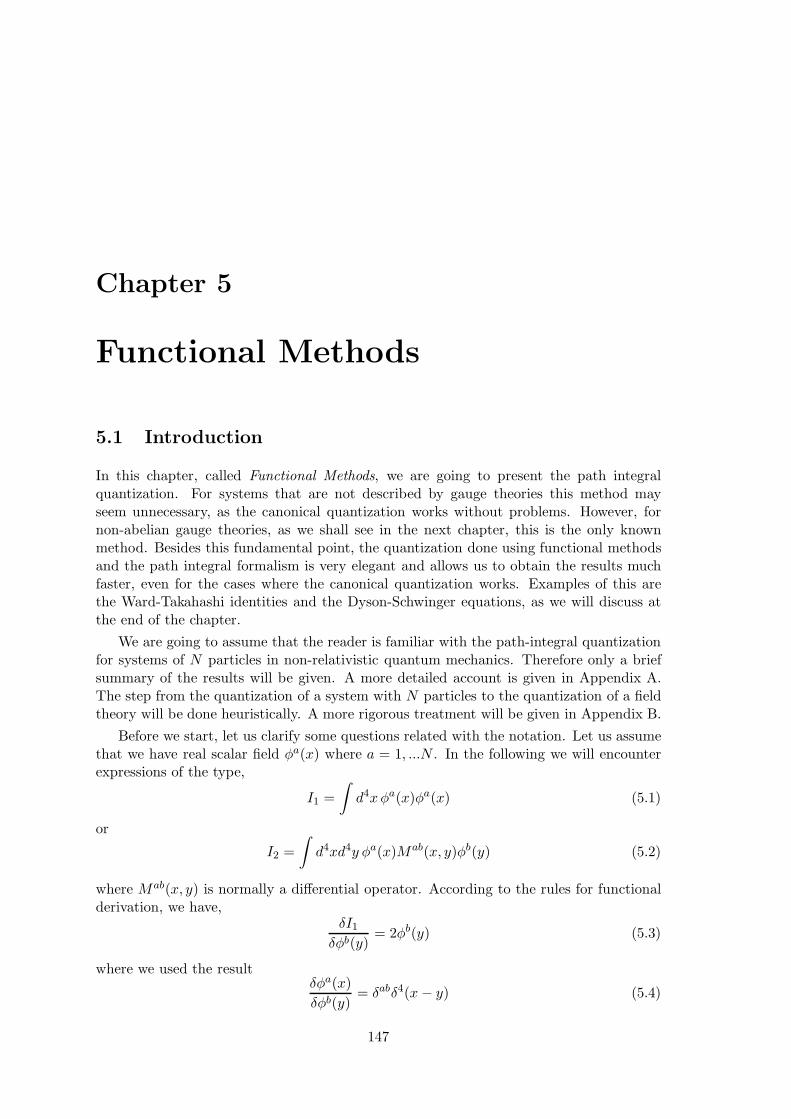
Chapter 5
Functional Methods
5.1 Introduction
In this chapter, called Functional Methods, we are going to present the path integralquantization. For systems that are not described by gauge theories this method mayseem unnecessary, as the canonical quantization works without problems. However, fornon-abelian gauge theories, as we shall see in the next chapter, this is the only knownmethod. Besides this fundamental point, the quantization done using functional methodsand the path integral formalism is very elegant and allows us to obtain the results muchfaster, even for the cases where the canonical quantization works. Examples of this arethe Ward-Takahashi identities and the Dyson-Schwinger equations, as we will discuss atthe end of the chapter.
We are going to assume that the reader is familiar with the path-integral quantizationfor systems of N particles in non-relativistic quantum mechanics. Therefore only a briefsummary of the results will be given. A more detailed account is given in Appendix A.The step from the quantization of a system with N particles to the quantization of a fieldtheory will be done heuristically. A more rigorous treatment will be given in Appendix B.
Before we start, let us clarify some questions related with the notation. Let us assumethat we have real scalar field φa(x) where a = 1, ...N . In the following we will encounterexpressions of the type,
I1 =
∫d4xφa(x)φa(x) (5.1)
or
I2 =
∫d4xd4y φa(x)Mab(x, y)φb(y) (5.2)
where Mab(x, y) is normally a differential operator. According to the rules for functionalderivation, we have,
δI1δφb(y)
= 2φb(y) (5.3)
where we used the resultδφa(x)
δφb(y)= δabδ4(x− y) (5.4)
147

148 CHAPTER 5. FUNCTIONAL METHODS
If we keep all the indices in the previous expressions (and in some much more compli-cated that we will encounter soon), we will get a very complicated situation with respectto the notation. Therefore it will be useful to make use of a more compact notation. Tothis end we identify,
φi ⇐⇒ φa(x) (5.5)
that is, the index i will represent both the discrete index a as well as the continuous x,
i⇐⇒ a, x (5.6)
In the case that the fields have further indices we will assume that i will always rep-resent them collectively. We also use the Einstein convention meaning a sum for discreteindices and an integration for continuous indices. With these conventions Eq. (5.1) andEq. (5.4) can be written as
I1 = φiφi I2 = φiMijφj
δI1δφj
= 2φjδφiδφj
= δij
(5.7)
In the following we will use these conventions, returning to the more usual notation whenconvenient or in case of a possible confusion.
5.2 Generating functional for Green’s functions
5.2.1 Green’s functions
The basic objects in Quantum Field Theory are the so-called Green functions. To avoidunnecessary complications we are going to use mostly the example of the scalar field. Thegeneralizations are however quite straightforward. The Green function of order n is givenby
G(n)(x1, . . . , xn) ≡ 〈0|Tφ(x1) · · · φ(xn)|0〉 . (5.8)
The Green functions defined in the previous equation are, sometimes called completeto distinguish from the Green functions connected, truncated or one particle irreduciblethat we now are going to define.
5.2.2 Connected Green’s functions
We call connected Green functions those that in which none of the external lines goesthrough the diagram without interacting. As an example, in Fig. 5.1 we represent adisconnected contribution to G4(x1, . . . , x4), while in Fig. 5.2 we have a connected contri-bution to the same Green function.
Therefore the connected Green functions are obtained summing over all the connecteddiagrams. The disconnected Green functions, corresponding to disconnected diagrams,can be obtained from connected Green functions of lower order, therefore the relevantquantities are the connected Green functions Gnc (x1, . . . , xn). It is clear that we have
Gnc (x1, . . . , xn) = Gn(x1, . . . , xn)− partes desconexas, (5.9)

5.2. GENERATING FUNCTIONAL FOR GREEN’S FUNCTIONS 149
x1 x2
x3 x4
Figure 5.1: Disconnected contribution to G4(x1, . . . , x4).
x1 x2
x3 x4
Figure 5.2: Connected contribution to G4(x1, . . . , x4).
andG2c(x1, x2) = G2(x1, x2) . (5.10)
Conventionally we represent Gnc (x1, . . . , xn) by the diagram of Fig. 5.3,
x1 x2
xixn
Figure 5.3: Graphical representation for Gnc (x1, . . . , xn).
Sometimes it is important to consider the Green functions in momentum space. Wedefine then Gnc (p1, . . . , pn) through the relation (Fourier Transform)
(2π)4δ4(p1 + p2 + · · · pn) Gnc (p1, . . . , pn)
≡∫d4x1 · · · d4xne−i(p1·x1+···+pn·xn) Gnc (x1, . . . , xn) , (5.11)
where all momenta, p1, . . . , pn, are incoming, as shown in Fig. 5.4. Notice that in thedefinition we have factored out the delta function that ensures the conservation of 4-momentum. With these conventions G2(p,−p) ≡ G2(p) is the full propagator representedin Fig. 5.5.

150 CHAPTER 5. FUNCTIONAL METHODS
p1 p2
pipn
Figure 5.4: Graphical representation for Gnc (p1, . . . , pn)
p −p
Figure 5.5: Full propagator G2(p).
5.2.3 Truncated Green’s functions
For n > 2 one defines the truncated Green functions through the relation,
Gntrunc(p1, . . . , pn) =
n∏
k=1
[G2(pk)
]−1Gnc (p1, . . . , pn) (5.12)
that is, we multiply each external line by the inverse of the full propagator correspondingto that line. These are the functions that play a fundamental role in the Theory, as thesethe ones that are related to the S matrix elements. In fact the LSZ reduction formula forscalars fields is
〈p1, . . . , pn out|q1, . . . , qℓ in〉 = 〈p1, . . . , pn in|S|q1, . . . , qℓ in〉 = disconnected terms
+(iZ−1/2
)n+ℓ ∫d4y1 · · · d4xℓ exp
[i
(n∑
k=1
pk · yk −ℓ∑
k=1
qk · xk)]
×(⊔⊓y1 +m2) · · · (⊔⊓xℓ +m2) 〈0|Tφ(y1) · · · φ(xℓ)|0〉c (5.13)
which gives
〈p1, . . . , pn out|q1, . . . , qℓ in〉 = 〈p1, . . . , pn in|S|q1, . . . , qℓ in〉 = disconnected terms
+Z−(n+ℓ)/2 (2π)4δ(∑
pi −∑
qj
)Gn+ℓtrunc(−p1, . . . ,−pn, q1, . . . , qℓ) (5.14)
5.2.4 Irreducible diagrams
We saw in 5.14 that the S elements related with the cross sections are expressed in terms oftruncated diagrams. Among the truncated Green functions there is an important subset.

5.3. GENERATING FUNCTIONALS FOR GREEN’S FUNCTIONS 151
These are the Green functions that correspond to the subset of one particle irreducible orproper that are the truncated diagrams that remain connected when one cuts any arbitraryinternal line. For instance the diagram of Fig. 5.61 is truncated but it is not proper, whilethe diagram of Fig. 5.7 is proper (in λφ3).
Figure 5.6: Example of a truncated diagram that is not proper.
Figure 5.7: Example of a proper diagram.
The reason why the non-irreducible truncated diagrams are not important is becausethey can always be expressed in terms of irreducible diagrams of lower order (remember theself energy series that we saw in the last lecture). It is convenient to introduce a notationfor the irreducible Green Functions (sum of all the irreducible diagrams for a given numberof exterior legs) where the factor i was introduced by convenience. In Fig. 5.8 the externallegs are drawn to make the figure more clear. They are in fact truncated. It is alsoconvenient to define a notation for the truncated diagrams of order n. This is shown inFig. 5.9 or, in another way, in Fig. 5.10. We can define similar diagrams in momentumspace.
5.3 Generating functionals for Green’s functions
The Generating Functional (FG) for the Green functions plays a very important role inQuantum Field Theory. In fact starting with it, by taking appropriate functional deriva-tives, one can obtain all the Green functions. Therefore they can treat simultaneously aninfinite number of Green functions. The FG of the full Green functions is given by,
Z(J) ≡⟨0|TeiJiφi |0
⟩(5.15)
1The bars indicate the the external lines are cuted.

152 CHAPTER 5. FUNCTIONAL METHODS
iΓ(n)(x1, . . . , xn) =
x1 x2
xixn
Figure 5.8: Irreducible Green functions.
G(n)trunc(x1, . . . , xn) ≡ ≡ =
x1x1 x2x2
xixi xnxn
Figure 5.9: Graphical representation of truncated Green functions.
where we are using the compact notation explained before.
Jiφi ≡∫d4x J(x)φ(x) . (5.16)
Z(J) generates all the Green functions, because if we expand the exponential in 5.15 weget
Z(J) =∑∞
n=0in
n!Ji1 · · · Jin 〈0|Tφi1 · · ·φin |0〉
=∑∞
n=0in
n!Ji1 · · · JinGni1···in (5.17)
The Green functions are then obtained taking derivatives
Gni1···in =δnZ
iδJi1 · · · iδJin
∣∣∣∣Ji=0
(5.18)
The generating functional of the connected Green functions is defined by the relation,
Z(J) = eiW (J) (5.19)

5.3. GENERATING FUNCTIONALS FOR GREEN’S FUNCTIONS 153
=
x1 x1x2 x2
xi xixn xn
Figure 5.10: Another representation of truncated Green functions.
orW (J) = −i lnZ(J) . (5.20)
The connected Green functions are then obtained by taking functional derivatives
Gnc i1···in = iδnW
iδJi1 · · · iδJin
∣∣∣∣Ji=0
(5.21)
Before we actually prove this statement, let us define the last important generating func-tional, the one that generates the irreducible Green functions. This is defined through theLegendre transformation of W (J), that is
Γ(φ) ≡W (J)− Jiφi (5.22)
where
φi ≡ δW (J)δJi
Ji = −δΓ(φ)δφi
(5.23)
The irreducible Green functions are then obtained through
Γni1···in =δnΓ(φ)
δφi1 · · · δφin
∣∣∣∣φ=0
. (5.24)
Having given the definitions we have now to show that W (J) and Γ(φ) do generate theconnected and irreducible Green functions, respectively. Let us start with W (J). Theproof is done calculating Gnc i1···in . We are going only to do only the n = 2, n = 3 andn = 4 cases. The generalizations are immediate.
n = 2
G2c i1i2 = i
δ2W
iδJi1 iδJi2
∣∣∣∣Ji=0
=δ2 lnZ
iδJi1 iδJi2
∣∣∣∣Ji=0
=δ
iδJi1
1
Z
δZ
iδJi2
∣∣∣∣Ji=0

154 CHAPTER 5. FUNCTIONAL METHODS
=1
Z
δ2Z
iδJi1 iδJi2
∣∣∣∣Ji=0
− 1
Z
δZ
iδJi1
1
Z
δZ
iδJi2
∣∣∣∣Ji=0
=δ2Z
iδJi1 iδJi2
∣∣∣∣Ji=0
(5.25)
orG2c i1i2 = G2
i1i2 (5.26)
To obtain this result we have used,
Z(0) = 1 The vacuum is normalized
δZ
iδJi= 〈0|Tφi|0〉 = 0 There is no symmetry breaking (5.27)
n = 3
G3c i1i2i3 =
[1
Z
δ3Z
iδJi1 iδJi2 iδJi3− 1
Z
δ2Z
iδJi1 iδJi2
1
Z
δZ
iδJi3
− 1
Z
δ2Z
iδJi2 iδJi3
1
Z
δZ
iδJi1− 1
Z
δ2Z
iδJi1 iδJi3
1
Z
δZ
iδJi2
+21
Z
δZ
iδJi1
1
Z
δZ
iδJi2
1
Z
δZ
iδJi3
]
|Ji=0
(5.28)
thereforeG3i1i2i3 = G3
c i1i2i3 (5.29)
The case n = 4 is left as an exercise (see Problem x.x). The extension to n > 4 isstraightforward. We have therefore showed that W (J) generates all the connected Greenfunctions. Let us now show that Γ(φ) is the generating functional for the irreducible Greenfunctions. For that we need two auxiliary results. The first one is based in the relation
δJiδJk
= δik (5.30)
This relation it is obvious. However one can obtain starting with it another importantrelation. In fact
δJiδJk
=δJiδφℓ
δφℓδJk
= − δ2Γ
δφiδφℓ
δ2W
δJℓδJk= −iΓiℓGℓk (5.31)
orΓiℓGℓk = iδik (5.32)
This fundamental relation expresses the fact that Γ2 is the inverse of the propagator(except for the i that comes from conventions). It is useful to write it in a diagrammaticform shown in 5.11. Notice that
iΓ(2)ik ≡ (5.33)
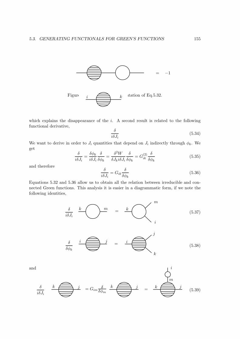
5.3. GENERATING FUNCTIONALS FOR GREEN’S FUNCTIONS 155
= −1
Figure 5.11: Graphical representation of Eq.5.32.i k
which explains the disappearance of the i. A second result is related to the followingfunctional derivative,
δ
iδJi(5.34)
We want to derive in order to Ji quantities that depend on Ji indirectly through φk. Weget
δ
iδJi=δφkiδJi
δ
δφk=
δ2W
δJkiδJi
δ
δφk= G
(2)ik
δ
δφk(5.35)
and thereforeδ
iδJi= Gik
δ
δφk(5.36)
Equations 5.32 and 5.36 allow us to obtain all the relation between irreducible and con-nected Green functions. This analysis it is easier in a diagrammatic form, if we note thefollowing identities,
δ
iδJi(5.37)
i
kk =
m
m
δ
δφk(5.38)
ii
k
=j
j
and
δ
iδJi(5.39)
i
kkk
m
jjj == Gimδ
δφm

156 CHAPTER 5. FUNCTIONAL METHODS
where we have used 5.36 to establish 5.39. In all these relations it is understood that atthe end (after taking the functional derivatives) we do J = 0 e φ = 0 at the right placesWe will use now these relations to relate the connected and irreducible Green functionsfor n = 3 and n = 4.
n = 3
The starting point is the equation 5.32. We apply δiδJℓ
to 5.32 and we get
δ
iδJℓ= 0 (5.40)i k
= 0
Using equations 5.37 and 5.39 we get the diagram of Figure 5.12.
ii k
k
l
l
+ = 0
Figure 5.12: Graphical result of Eq.5.40.
Multiplying on the left by G(2)mi and using 5.32 we get
iΓ(3)mkl ≡
(5.41)
mm
k
k
l
l
=
This shows that Γ(3)mkl is in fact the irreducible Green function with 3 external legs, as for
3 external legs the irreducible and truncated Green functions coincide. To show that wehave really irreducible functions and not only truncated ones, one has to go to n = 4 asthe difference starts there.
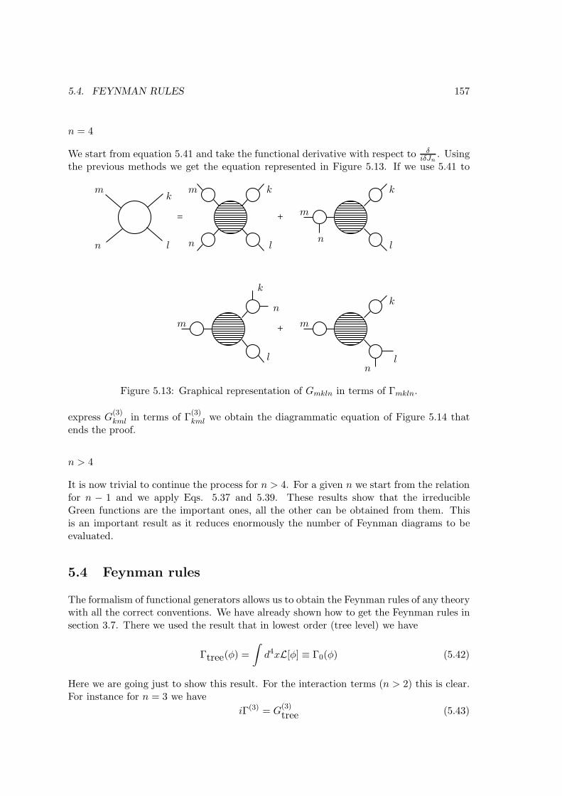
5.4. FEYNMAN RULES 157
n = 4
We start from equation 5.41 and take the functional derivative with respect to δiδJn
. Usingthe previous methods we get the equation represented in Figure 5.13. If we use 5.41 to
= +
+ mm
m
m
m
k
k
k kk
ll
l ll
n
n
n nn
Figure 5.13: Graphical representation of Gmkln in terms of Γmkln.
express G(3)kml in terms of Γ
(3)kml we obtain the diagrammatic equation of Figure 5.14 that
ends the proof.
n > 4
It is now trivial to continue the process for n > 4. For a given n we start from the relationfor n − 1 and we apply Eqs. 5.37 and 5.39. These results show that the irreducibleGreen functions are the important ones, all the other can be obtained from them. Thisis an important result as it reduces enormously the number of Feynman diagrams to beevaluated.
5.4 Feynman rules
The formalism of functional generators allows us to obtain the Feynman rules of any theorywith all the correct conventions. We have already shown how to get the Feynman rules insection 3.7. There we used the result that in lowest order (tree level) we have
Γtree(φ) =
∫d4xL[φ] ≡ Γ0(φ) (5.42)
Here we are going just to show this result. For the interaction terms (n > 2) this is clear.For instance for n = 3 we have
iΓ(3) = G(3)
tree (5.43)

158 CHAPTER 5. FUNCTIONAL METHODS
= +
+ +
m
m
mm
m
k
k
kk
k
ll
ll
l
nn
nn
n
Figure 5.14: Graphical representation of Gmkln in terms of Γmkln.
while for n = 4 we getiΓ(4) = G(4) − irreducible parts (5.44)
and it is obvious that iΓ(4)tree generates the vertices.
The i factor is in agreement with the usual conventions for the Feynman rules as itcomes from the term exp
(i∫d4xLint
)in the calculation of the Green functions. For the
quadratic terms we have, Eq. 5.32,
Γ(2)
tree(p) = p2 −m2 (5.45)
therefore, doing the inverse Fourier transform,
Γ(2)
tree(x, y) =
∫d4p1(2π)4
d4p2(2π)4
ei(p1·x+p2·y)(2π)4δ4(p1 + p2) (p21 −m2) (5.46)
and
1
2
∫d4xd4y φ(x)Γ
(2)
tree(x, y)φ(y) =
=1
2
∫d4xd4y
d4p1(2π)4
d4p2(2π)4
ei(p1·x+p2·y)(2π)4δ(p1 + p2)(p21 −m2)φ(x)φ(y)
=1
2
∫d4xφ(x)(−⊔⊓ −m2)φ(x) =
1
2
∫d4x
(∂µφ∂
µφ−m2φ2)
(5.47)
which shows that Γtree is in fact the action. In getting to Eq. (5.47) we have done anintegration by parts and discarded, usual, the boundary term. We refer the reader toSection 3.7 for the actual recipes on how to determine the Feynman rules of any theory.

5.5. PATH INTEGRAL FOR GENERATING FUNCTIONALS 159
5.5 Path integral for generating functionals
5.5.1 Quantum mechanics of n degrees of freedom
Let us start reviewing the results for the path integral in systems with 1 degree of freedom.In appendix A a more detailed explanation is given for the results that we are going touse. The fundamental result is the following transition amplitude,
⟨q′; t′|q; t
⟩= N
∫D(q)ei
∫ t′
tdtL(q,q) = N
∫D(q)eiS (5.48)
whereN is a normalization factor and D(q) is a symbolic form for representing the measureof integration. This is in fact a complicated limit (see appendix A). Another importantresult concerns the time ordered matrix elements of operators. Let
O(t1, . . . , tn) = T [OH1 (t1)OH2 (t2)...O
Hn (tn)] (5.49)
such thatt′ ≥ (t1, t2, . . . , tn) ≥ t (5.50)
Then ⟨q′; t′
∣∣O(t1, . . . , tn) |q; t〉 = N
∫D(q)O1(q(t1)) · · ·On(q(tn))eiS (5.51)
where we have assumed that the operators Oi are diagonal in the coordinate space. Forthe generalization to Quantum Field Theory the important objects are not the transitionamplitudes but the generating functionals. Consider, for instance, the Green function
G(t1, t2) ≡ 〈0|T (QH(t1)QH(t2)) |0〉 (5.52)
where |0〉 is the ground state and QH(t) is the coordinate operator in the Heisenbergrepresentation. To write Eq. (5.52) using the path integral, we introduce a complete setof states and we write
G(t1, t2) =
∫dq dq′
⟨0|q′; t′
⟩ ⟨q′; t′
∣∣T (QH(t1)QH(t2)) |q; t〉 〈q; t|0〉
=
∫dqdq′φ0(q
′, t′)φ∗0(q, t)∫
D(q)q(t1)q(t2)ei∫ t′
tLdτ (5.53)
whereφ0(q, t) = 〈0|q; t〉 = φ0(q)e
−iE0t (5.54)
The appearance in this expression of the wave functions of the fundamental state makesthe expression not very useful. We can remove them in the following way. Consider thematrix element
⟨q′; t′
∣∣O(t1, t2) |q; t〉
=
∫dQ dQ′
⟨q′; t′|Q′;T ′
⟩ ⟨Q′;T ′
∣∣O(t1, t2) |Q;T 〉 〈Q;T |q; t〉 (5.55)
where
O(t1, t2) = T (QH(t1)QH(t2))

160 CHAPTER 5. FUNCTIONAL METHODS
t′ ≥ T ′ ≥ (t1, t2) ≥ T ≥ t (5.56)
Let |n〉 be the eigenstates of energy En with wave function φn(q) that is
H |n〉 = En |n〉〈q|n〉 = φ∗n(q) (5.57)
Then
⟨q′; t′|Q′;T ′
⟩=
⟨q′∣∣ e−iH(t′−T ′)
∣∣Q′⟩
=∑
n
⟨q′|n
⟩〈n| e−iH(t′−T ′)
∣∣Q′⟩
=∑
n
φ∗n(q′)φn(Q
′)e−iEn(t′−T ′) (5.58)
We consider now the limit t′ → −i∞. We obtain then
limt′→−i∞
⟨q′; t′|Q′;T ′
⟩= φ∗0(q
′)φ0(Q′)e−E0|t′|eiE0T ′
(5.59)
In a similar way
limt→i∞
〈Q;T |q; t〉 = φ0(q)φ∗0(Q)e−E0|t|e−iE0T (5.60)
Applying these limits to Eq. (5.55) we get
limt′→−i∞
limt→i∞
⟨q′; t′
∣∣O(t1, t2) |q; t〉
=
∫dQdQ′φ∗0(q
′)φ0(Q′)e−E0|t′|eiE0T ′
⟨Q′;T ′
∣∣O(t1, t2) |Q;T 〉φ0(q)φ∗0(Q)e−E0|t|e−iE0T
= φ∗0(q′)φ0(q)e
−E0|t′|e−E0|t|
∫dQdQ′φ0(Q
′, T ′)φ∗0(Q,T )⟨Q′;T ′
∣∣O(t1, t2) |Q;T 〉 (5.61)
Using the definition of Green function in Eq.5.53 we obtain the important result
limt′→−i∞
limt→i∞
⟨q′; t′
∣∣O(t1, t2) |q; t〉 = φ∗0(q′)φ0(q)e
−E0|t′|e−E0|t|G(t1, t2) (5.62)
On the other hand
limt′→−i∞
limt→i∞
⟨q′; t′|q; t
⟩= φ∗0(q
′)φ0(q)e−E0|t′|eE0|t| (5.63)
Therefore we can finally write
G(t1, t2) = limt′→−i∞
limt→i∞
[〈q′; t′|T (QH(t1)QH(t2)) |q; t〉〈q′; t′|q; t〉
](5.64)

5.5. PATH INTEGRAL FOR GENERATING FUNCTIONALS 161
Using 5.51 we can finally write G(t1, t2) in terms of a path integral, as
G(t1, t2) = limt′→−i∞
limt→i∞
1
〈q′; t′|q; t〉
∫D(q)q(t1)q(t2)e
i∫ t′
tLdτ (5.65)
This result is easily generalized to Green functions with n-points
G(t1, . . . , tn) = 〈0|T (q(t1) · · · q(tn)) |0〉
= limt′→−i∞
limt→i∞
1
〈q′; t′|q; t〉
∫D(q)q(t1) · · · q(tn)ei
∫ t′
tLdτ (5.66)
We can now see that all the Green functions can be obtained from the generating functional
Z[J ] = limt′→−i∞
limt→i∞
1
〈q′; t′|q; t〉
∫D(q)ei
∫ t′
t[L(q,q)+Jq]dτ (5.67)
by functional derivation
G(t1, . . . , tn) =δnZ[J ]
iδJ(t1) · · · iδJ(tn)
∣∣∣∣J=0
(5.68)
The expression 5.67 for the generating functional shows that its the transition amplitudebetween the ground state at time t and the ground state at time t′, in the presence of anexterior source and with normalization such that Z[J = 0] = 1
Z[J ] = 〈0|0〉J (5.69)
For a system with n degrees of freedom, we have the generalization of 5.67
Z[J1, . . . , Jn] = limt′→−i∞
limt→i∞
N
∫D(qi)e
i∫ t′
tdτ [L(qi,qi)+
∑Ni=1 Jiqi] (5.70)
Comments
• In the previous equation the time limits for times t and t′ are imaginary. This meansthat these Green functions are in Euclidean space. For field theory this correspondsto the prescription m2 → m2 − iǫ.
• In equation 5.70 we do not explicitly wrote the normalization. It should be chosenin such a way that Z[0, . . . , 0] = 1. However, as we will see, for the connectedGreen functions in Quantum Field Theory the normalization it is not relevant, andtherefore we will not worry about it.
5.5.2 Field theory
To get the generating functional in Quantum Field Theory we proceed in the usual heuristicway, by making the following equivalences,
t → xµ

162 CHAPTER 5. FUNCTIONAL METHODS
q(t) → φ(x)
D(q) → D(φ)
L(qi, qi) →∫d3xL(φ, ∂µφ) (5.71)
We get therefore
Z[J ] = N
∫D(φ)ei
∫
d4x[L(φ,∂µφ)+J(x)φ(x)] (5.72)
This is the starting point in the path integral quantization. We will see in the next lecturehow to use it. A more rigorous derivation of the above result, Eq. 5.72, be found inappendix B.
5.5.3 Applications
Once we know the generating functional Z[J ] we also know all the Green functions of thetheory and therefore how to address any problem in Quantum Field Theory. We can askin which conditions can we evaluate Z[J ]? The answer is that as we only know how to doGaussian path integrals we can only do either free fields or perturbation theory. Howeverthere are two main advantages in the method that we will now discuss:
• Perturbation Theory
The expression for Z[J ] allows to establish the perturbative expansion and find theFeynman rules for any theory.
• Formal Manipulations
Relations among the Green functions that are a consequence of symmetry propertiesof the theory (for instance Ward identities) are much simpler in terms of the gener-ating functionals. Here the expression of Z[J ] in terms of a path integral, Eq. 5.72is particularly useful as we will discuss later.
We will use the scalar field as an example to illustrate the first point, that is how toestablish the perturbative expansion. We consider a real scalar field, described by theLagrangian,
L(φ) = L0(φ) + LI(φ) (5.73)
where L0(φ) is quadratic in the fields, that is
L0(φ) =1
2∂µφ∂
µφ− 1
2m2φ2 (5.74)
We can then write,
Z[J ] = N
∫D(φ)ei
∫
d4x[L0(φ)+LI (φ)+Jφ]
= N
∫D(φ)ei
∫
d4x[LI(φ)] ei∫
d4x[L0(φ)+Jφ] (5.75)
This last integral can formally be written in the form,
Z[J ] = exp
[i
∫d4xLI
(δ
iδJ
)]Z0[J ] (5.76)

5.5. PATH INTEGRAL FOR GENERATING FUNCTIONALS 163
where
Z0[J ] = N
∫D(φ)ei
∫
d4x[L0+Jφ] . (5.77)
The usefulness of this expression results from the two following points:
• Z0[J ] can be exactly calculated because is quadratic in the fields (Gaussian integral).
• If LI(φ) has a small parameter, the exponential can be developed in a power seriesin this parameter and the generating functional Z[J ] can be obtained order by orderin perturbation theory, as the integrals will be Gaussian integrals with polynomials.
5.5.4 Example: perturbation theory for λφ4
To see the connection with the usual results let us consider as an example the derivationof the Feynman rules for a real scalar theory with the interaction,
LI = − λ
4!φ4 . (5.78)
The generating functional Z[J ] is
Z[J ] = N exp
(−iλ) 1
4!
∫d4x
(δ
iδJ
)4Z0[J ] (5.79)
where (see Problems)
Z0[J ] = exp
−1
2
∫d4xd4yJ(x)∆(x, y)J(y)
(5.80)
The normalization N is to be chosen such that Z[0] = 1, as we will see later. We expandin a series in the coupling constant,
Z[J ] = NZ0[J ]1 + (−iλ)Z ′1[J ] + (−iλ)2Z ′2[J ] + · · ·
(5.81)
where
Z ′1[J ] ≡ Z−10 [J ]
1
4!
∫d4x
(δ
δJ
)4Z0[J ] (5.82)
and
Z ′2[J ] ≡ 1
2Z−10 [J ]
1
4!
∫d4x
(δ
δJ
)42
Z0[J ]
=1
2Z−10 [J ]
1
4!
∫d4x
(δ
δJ
)4(Z0Z
′1)
=1
2
(Z ′1[J ]
)2+
1
2Z−10 [J ]
1
4!
∫d4x
4δ3Z0
δJ3(x)
δZ ′1δJ(x)

164 CHAPTER 5. FUNCTIONAL METHODS
+6δ2Z0
δJ2(x)
δ2Z ′1δJ2(x)
+ 4δZ0
δJ(x)
δ3Z ′1δJ3(x)
+ Z0δ4Z ′1δJ4(x)
(5.83)
We get for the first order
Z ′1[J ] =
=1
4!
∫d4x
[3∆(x, x)∆(x, x) − 3!∆(x, x)
∫d4y1d
4y2∆(x, y1)∆(x, y2)J(y1)J(y2)
+
∫d4y1 · · · d4y4∆(x, y1)∆(x, y2)∆(x, y3)∆(x, y4)J(y1)J(y2)J(y3)J(y4)
](5.84)
This result can be represented diagrammatically in the form,
Z ′1 =1
8− 1
4+
1
4!(5.85)
For Z ′2 we get
Z ′2[J ]
=1
2
(Z ′1[J ]
)2+
1
2
(1
4!
)2
4!
∫d4x1d
4x2∆(x1, x2)∆(x1, x2)∆(x1, x2)∆(x1, x2)
+
(1
4!
)2 [−72
∫d4x2
∫d4x1∆(x1, x2)
∫d4y1∆(x1, y1)J(y1)
∆(x1, x2)∆(x2, x2)
∫d4y2∆(x2, y2)J(y2)
+24
∫d4x2d
4x1∆(x1, x1)
∫d4y1∆(x1, y1)J(y1)∆(x1, y2)
∫d4y2∆(x2, y1)J(y2)
∫d4y3∆(x2, y3)J(y2)
∫d4y4∆(x1, y4)J(y4)
+24
∫d4x2
∫d4x1
∫d4y1d
4y2d4y3d
4y4∆(x1, x2)∆(x1, y1)
∆(x1, y2)∆(x1, y2)∆(x2, x2)∆(x2, y4)J(y1) · · · J(y4)
−8
∫d4x2
∫d4x1
∫d4y1 · · · d4y6∆(x1, x2)∆(x1, y1)∆(x1y2)
∆(x1, y3)∆(x2, y4)∆(x2, y5)∆(x2, y6)J(y1) · · · J(y6)
+36
∫d4x2d
4x1∆(x1, x1)∆(x1, x2)∆(x1, x2)∆(x2, x2)

5.5. PATH INTEGRAL FOR GENERATING FUNCTIONALS 165
−36
∫d4x2d
4x1∆(x1, x1)∆(x1, x2)∆(x1, x2)
∫d4y1d
4y2∆(x2, y1)
∆(x2, y2)J(y1)J(y2)
−36
∫d4x2d
4x1d4y1d
4y2∆(x1, x2)∆(x1, x2)∆(x2, x1)
∆(x1, y1)∆(x1, y2)J(y1)J(y2)
+36
∫d4x2d
4x1d4y1 · · · d4y4∆(x1, x2)∆(x1, x2)∆(x1, y1)
∆(x1, y2)∆(x2, y3)∆(x2, y4)J(y1) · · · J(y4)
−48
∫d4x2dy1d
4y1d4y2∆(x1, x2)∆(x1, x2)∆(x1, x2)
∆(x1, y1)∆(x2, y2)J(y1)J(y2)
](5.86)
This can also be written as,
Z ′2[J ]
=1
2
(Z ′1[J ]
)2+
1
2 · 4!
∫d4x1d
4x2∆4(x1, x2)
+3
2 · 4!
∫d4x1d
4x2∆(x1, x1)∆2(x1, x2)∆(x2, x2)
− 1
2 · 3! · 3!
∫d4x1d
4x2d4y1 · · · d4y6∆(y1, x1)∆(y2, x1)∆(y3, x1)
∆(x1, x2)∆(x2, y4)∆(x2, y5)∆(x2, y6)J(y1) · · · J(y6)
+2
4!
∫d4x1d
4x2d4y1 · · · d4y4∆(y1, x1)∆(x1, x1)∆(x1, x2)
∆(x2, y2)∆(x2, y3)∆(x2, y4)J(y1) · · · J(y4)
+3
2 · 4!
∫d4x1d
4x2d4y1 · · · d4y4∆(y1, x1)∆(y2, x1)∆
2(x1, x2)
∆(x2, y3)∆(x2, y4)J(y1) · · · J(y4)
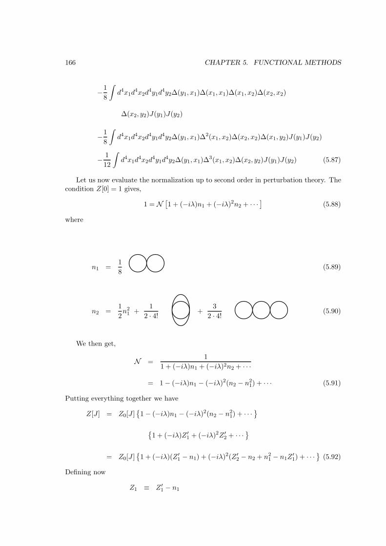
166 CHAPTER 5. FUNCTIONAL METHODS
−1
8
∫d4x1d
4x2d4y1d
4y2∆(y1, x1)∆(x1, x1)∆(x1, x2)∆(x2, x2)
∆(x2, y2)J(y1)J(y2)
−1
8
∫d4x1d
4x2d4y1d
4y2∆(y1, x1)∆2(x1, x2)∆(x2, x2)∆(x1, y2)J(y1)J(y2)
− 1
12
∫d4x1d
4x2d4y1d
4y2∆(y1, x1)∆3(x1, x2)∆(x2, y2)J(y1)J(y2) (5.87)
Let us now evaluate the normalization up to second order in perturbation theory. Thecondition Z[0] = 1 gives,
1 = N[1 + (−iλ)n1 + (−iλ)2n2 + · · ·
](5.88)
where
n1 =1
8(5.89)
n2 =1
2n21 +
1
2 · 4! +3
2 · 4! (5.90)
We then get,
N =1
1 + (−iλ)n1 + (−iλ)2n2 + · · ·
= 1− (−iλ)n1 − (−iλ)2(n2 − n21) + · · · (5.91)
Putting everything together we have
Z[J ] = Z0[J ]1− (−iλ)n1 − (−iλ)2(n2 − n21) + · · ·
1 + (−iλ)Z ′1 + (−iλ)2Z ′2 + · · ·
= Z0[J ]1 + (−iλ)(Z ′1 − n1) + (−iλ)2(Z ′2 − n2 + n21 − n1Z
′1) + · · ·
(5.92)
Defining now
Z1 ≡ Z ′1 − n1

5.5. PATH INTEGRAL FOR GENERATING FUNCTIONALS 167
Z2 ≡ Z ′2 − n2 + n21 − n1Z′1 = Z ′2 − n2 − n1Z1 (5.93)
we get
Z1[J ] = −1
4+
1
4!(5.94)
and
Z2[J ]
=1
2(Z1[J ])
2 +−1
2! 3! 3!
+3
2! 4!+
2
4!
−1
8− 1
8− 1
12(5.95)
with Z1[0] = Z2[0] = 0. Therefore the generating functional
Z[J ] = Z0[J ]1 + (−iλ)Z1[J ] + (−iλ)2Z2[J ] + · · ·
(5.96)
is automatically correctly normalized if we neglect all the vacuum amplitudes, know asbubbles. To verify that this expression reproduces the perturbation theory results, let usevaluate the propagator up to second order in λ2. We get
∆′(x1, x2) =δ2Z[J ]
iδJ(x1)iδJ(x2)
∣∣∣∣J=0
= − δ2Z0[J ]
δJ(x1)δJ(x2)
∣∣∣∣J=0
− (−iλ) δ2Z1[J ]
δJ(x1)δJ(x2)
∣∣∣∣J=0
− (−iλ)2 δ2Z2[J ]
δJ(x1)δJ(x2)
∣∣∣∣J=0

168 CHAPTER 5. FUNCTIONAL METHODS
= ∆(x1, x2) + (−iλ)12
∫d4y∆(x1, y)∆(x2, y)∆(y, y)
+(−iλ)2∫d4y1d
4y2
[1
4∆(x1, y1)∆(y1, y1)∆(y1, y2)∆(y2, y2)∆(y2, x2)
+1
4∆(x1, y1)∆
2(y1, y2)∆(y2, y2)∆(y1, x2) +1
6∆(x1, y1)∆
3(y1, y2)∆(y2, x2)
](5.97)
In diagrammatic form we have the situation of Figure 5.15.
=
x1x1x1
x1x1x1
x2x2x2
x2x2x2+
1
2
+1
4+
1
4+
1
6
Figure 5.15:
Continuing with the scalar λφ4 theory as an example, let analyze the generating func-tional for the connected Green functions, W [J ]. It is easy to see that the terms likeZ21 [J ] correspond to disconnected diagrams which are part of Z[J ]. Let us see how they
disappear in W [J ]. We have
iW [J ] = lnZ[J ] =
= lnZ0[J ] + ln1 + (−iλ)Z1[J ] + (−iλ)2Z2[J ] + · · ·
= iW0[J ] + (−iλ)Z1[J ]−1
2(−iλ)2 (Z1[J ])
2 + (−iλ)2Z2[J ] + · · ·
= iW0[J ] + (−iλ)Z1[J ] +
(−iλ)2(Z2[J ]−
1
2(Z1[J ])
2
+ · · ·
≡ iW0[J ] + (−iλ)W1[J ] + (−iλ)2W2[J ] + · · ·
(5.98)
with
iW1[J ] = Z1[J ], iW2[J ] = Z2[J ]−1
2(Z1[J ])
2 (5.99)
Therefore the disconnected diagrams contained in Z2[J ] are subtracted and W1 and W2
have only the connected diagrams.
5.5.5 Symmetry factors
After doing the derivatives in order to J to obtain a given Green function, we have somediagrams multiplied by numbers known as symmetry factors. For instance for the one-loop

5.5. PATH INTEGRAL FOR GENERATING FUNCTIONALS 169
correction to the propagator we get,
∆′(x1, x2) =δ2Z
iδJ(x1)iδJ(x2)
∣∣∣∣J=0
=
=δ2Z0
iδJ(x1)iδJ(x2)
∣∣∣∣J=0
+ (−iλ) δ2Z1
iδJ(x1)iδJ(x2)
∣∣∣∣J=0
+ · · ·
= ∆(x1, x2) +1
2+ · · · (5.100)
The factor 12 is the symmetry factor that corresponds to that diagram. The method of
the generating functional gives automatically the correct symmetry factors. However inpractical applications it is normally easier to have a rule to obtain these symmetry factors.
Rule for the Symmetry Factors
The symmetry factor S of a diagram it is given by
S =N
D(5.101)
where N is the # of different ways of forming the diagram, and D it is the product of thesymmetry factors of each vertex by the number of permutations of equal vertices.
As an example take the diagram that contributes to the propagator at one-loop rep-resented in Fig. 5.16. Then according to the rule we have,
pp
Figure 5.16:
S =4× 3
4!=
1
2(5.102)
5.5.6 A comment on the normal ordering
In the previous example we have diagrams like in Fig. 5.16, that we generically denoteby “tadpoles”, that connect fields that belong to the same vertex, and that we saw thatwere excluded by the normal ordering. This difference comes from the fact that we were
170 CHAPTER 5. FUNCTIONAL METHODS
not very rigorous in the definition of the Lagrangian to include in the path formalism.If we would we would concluded that we should have to do the normal ordering in theLagrangian to include in ei
∫
d4xL(φ) This would make the Lagrangian L(φ) to include inthe path integral different from the classical Lagrangian. Let us look at φ4 as an example.We will use the relations
φ(x)φ(x) =: φ(x)φ(x) : + 〈0| φ(x)φ(x) |0〉 (5.103)
or symbolically: φ2 := φ2 − 〈0| φ2 |0〉 . (5.104)
In a similar way
φ4 =: φ4 : +6 : φ2 : 〈0| φ2 |0〉+ 6 〈0| φ2 |0〉 〈0| φ2 |0〉 (5.105)
Therefore we get
: φ4 := φ4 − 6 : φ2(x) : 〈0| φ2(x) |0〉 − 6(〈0| φ2 |0〉
)2(5.106)
or: φ4 := φ4 − 6 φ2 〈0| φ2 |0〉 (5.107)
This means that the quantum Lagrangian should be written as
LQInt = − λ
4!: φ4 :
= − λ
4!φ4 +
λ
4φ2I (5.108)
where
I ≡ 〈0| φ2(x) |0〉
=
∫˜dk1 ˜dk2 〈0|
(a†(k1)e
ik1·x + a(k1)e−ik1·x
)(a†(k2)e
ik2·x + a(k2)e−ik2·x
)|0〉
=
∫˜dk1 ˜dk2 〈0| a(k1)a†(k2) |0〉 ei(k2−k1)·x
=
∫˜dk1 =
∫d3k
(2π)31
2ωk(5.109)
In the previous expression we have used the relations
[a(k), a+(k′)
]= (2π)32ωkδ
3(~k − ~k′) (5.110)
ωk =
√k20 + |~k|2 (5.111)
The integral I is divergent and in fact it is equal to the one-loop integral. In fact
∫d4k
(2π)4i
k2 −m2 + iε

5.5. PATH INTEGRAL FOR GENERATING FUNCTIONALS 171
=
∫d3k
(2π)3
∫ +∞
−∞dk0
i
(k0 − ωk)(k0 + ωk)
=
∫d3k
(2π)31
2ωk= I (5.112)
Therefore if we had been rigorous we should have to include the term, λ4φ
2I in theinteraction. The Lagrangian to use in the path integral should then be,
LICInt = − λ
4!φ4 +
λ
4φ2I (5.113)
It is easy to verify that the additional term cancels the tadpole. In fact we have
=i
p2 −m2
[−iλ
2I + i
λ
2I
]i
p2 −m2
= 0 (5.114)
1/2+ =
and therefore the tadpoles would not appear. However many times we do not worry aboutthis considerations and just use the classical Lagrangian in the path integral. This can bedone because the tadpole gives an infinite contribution to the mass, that can be absorbedin the renormalization process.
In QED the same occurs, we should have as interaction Lagrangian
LICInt = −eψγµψAµ + eAµ 〈0|ψγµψ |0〉 (5.115)
and the second term would remove the tadpole shown in Fig. 5.17,
Figure 5.17: Tadpole for QED.
However, due the Lorentz invariance of the theory, one can show that this tadpole vanishesto all orders and therefore we do have to worry, just use the classical Lagrangian.

172 CHAPTER 5. FUNCTIONAL METHODS
5.5.7 Generating functionals for fermions
For theories with fermion fields we introduce Grassmann variables. These anti-commutingvariables are in some sense the the classical limit of fermionic quantum fields. The detailsof this construction are explained in the Appendices A and B. Here we just review ourconventions. Due to the anti-commuting character it is necessary to specify the order ofthe derivatives.
We will take the convention that derivatives are left derivatives, that is they obey,
δ
δη(x)
∫d4yη(y)ψ(y) = ψ(x)
δ
δη(x)
∫d4yψ(y)η(y) = −ψ(x) (5.116)
In the Green functions the order of the derivatives is such that
G2n(x1, . . . , yn) = 〈0|Tψ(x1) · · ·ψ(xn)ψ(y1) · · ·ψ(yn) |0〉
≡ δ2nZ[η, η]
iδη(yn) · · · iδη(y1)iδη(xn) · · · iδη(x1)
≡ δ
iδη(yn)· · · δ
iδη(x1)Z[η, η] (5.117)
where we have defined the generating functional for fermion fields as
Z[η, η] = 〈0|Tei∫
d4x[η(x)ψ(x)+ψ(x)η(x)] |0〉
=
∫D(ψ,ψ)ei
∫
d4x[L+η(x)ψ(x)+ψ(x)η(x)] (5.118)
Examples of these results will be given in the Problems at the end of the chapter.
5.6 Change of variables in path integrals. Applications
5.6.1 Introduction
One of the great advantages of having an expression for the generating functional Z[J ] interms of a path integral is that a great number of manipulations that are familiar for theusual integrals, (change of variables, integration by parts, ...) can also be applied here.Let us see the implications of changing integration variables.
Let us consider an infinitesimal transformation of the form,
φi → φi + εFi(φ) (5.119)
whereFi(φ) = fi + fijφj + · · · (5.120)
5.6. CHANGE OF VARIABLES IN PATH INTEGRALS. APPLICATIONS 173
Then we should have, in first order,
D(φ) → D(φ) det∣∣∣δij + ε δFiδφj
∣∣∣
= D(φ)(1 + ε δFiδφi
)(5.121)
On the other hand
ei(S(φ)+Jiφi) → ei(S(φ)+Jiφi)[1 + iε
(δS
δφi+ Ji
)Fi(φ)
](5.122)
As the integral for Z(J) should be independent of the change of variables we get
0 =
∫D(φ)
[i
(δS
δφi+ Ji
)Fi +
δFiδφi
]ei(S[φ]+Jiφi) (5.123)
Using φi → δiδJi
we get a more compact expression,
i
[δS
δφi
(δ
iδJi
)+ Ji
]Fi
(δ
iδJi
)+δFiδφi
(δ
iδJ
)Z(J) = 0 (5.124)
This the general expression that we are going to apply to two important particular cases,the Dyson-Schwinger equations and the Ward identities.
5.6.2 Dyson-Schwinger equations
Let Fi = fi independent of φi, that is a simple translation of the fields. Then the previousmaster equation simplifies to
(δS
δφi
[δ
iδJ
]+ Ji
)Z(J) = 0 (5.125)
We will see below that this the expression for the Dyson-Schwinger (DS) equations forthe generating functional of the full Green functions. In this way, the DS equations are aconsequence of the path integral for constant field translations. This equations can furtherbe written as
Jk = − 1
ZE
[δ
iδJk
]Z[J ] (5.126)
where the functional E[φ] is the Euler-Lagrange equation of motion,
E [φk] ≡δS
δφk. (5.127)
For many applications it is more convenient to write the Dyson-Schwinger equationsfor the connected and proper (one particle irreducible) Green functions. For this we haveto write the corresponding equations for the functional W and Γ. Using the identity
1
Z
δ
iδJk(Z[J ]f [J ]) =
(δiW
iδJk+
δ
iδJk
)f [J ] (5.128)

174 CHAPTER 5. FUNCTIONAL METHODS
we can write1
ZE
[δ
iδJk
]Z[J ] = E
[iδW
iδJk+
δ
iδJk
]1 (5.129)
Therefore the DS equation for the generating functional of the connected Green functionscan be written as,
Jk = −E[iδW
iδJk+
δ
iδJk
]1 (5.130)
Let us now find the corresponding equation for the proper, or one particle irreducible,Green functions. To obtain this equation we use the following relations
φk =i δW
iδJkJk = − δΓ
δφkδ
iδJk= Gkm
δ
δφm
δ
δφk= −iΓkr
δ
iδJr
We getδΓ
δφk= E
[φk +Gkm
δ
δφm
]1 (5.131)
It is in the form of Eq. 5.131, that the DS are more useful.
Example : Self-energy in φ3
Let us start with the example of the self-energy in φ3. The action for this theory is, usingour compact notation,
S[φ] =1
2φk(−⊔⊓ −m2)δkmφm − λ
3!(φk)
3 (5.132)
Therefore the equation of motion is
E[φk] = (−⊔⊓ −m2)φk −λ
2(φk)
2 (5.133)
We get therefore, expanding the functional,
E
[φk +Gkm
δ
δφm
]1 = −(⊔⊓+m2)φk −
λ
2
(φk +Gkr
δ
δφr
)φk (5.134)
We get therefore for the DS equation
δΓ
δφk= −(⊔⊓+m2)φk −
λ
2
(φ2k +Gkrδrk
)(5.135)
By taking functional derivatives with respect to φm we get the DS for the various Greenfunctions, all derived from just one master equation. For instance, for the self-energy weget,
δ2Γ
δφkδφm= −(⊔⊓+m2)δkm − λ
2(2φkδkm − iΓmnGkrnδrk) (5.136)

5.6. CHANGE OF VARIABLES IN PATH INTEGRALS. APPLICATIONS 175
Setting φk = 0 we get
Γkm − (−⊔⊓−m2)δkm = iλ
2ΓmnGkrnδrk
=λ
2ΓmnGkrnΓrsGsk
= iλ
2ΓmnΓrsGskGkk′Grr′Gnn′Γk′r′n′
= −iλ2Gkk′GksΓk′sm (5.137)
where we have repeatedly used the relation
ΓijGjk = iδik (5.138)
By definition of self-energy we have,
Γkm − (−⊔⊓ −m2)δkm ≡ −Σkm (5.139)
Therefore
−iΣkm = −iλ2Gkk′GksiΓk′sm (5.140)
as shown in the Fig. 5.18, We see that the DS equation is no more than the statement
=kk mm
Figure 5.18: Dyson-Schwinger equation for φ3.
that the vertex of the theory is λ3!φ
3.
Example: Self-energy in φ4
In the case the action is
S[φ] =1
2φk(−⊔⊓−m2)δkmφm − λ
4!(φk)
4 . (5.141)
Therefore the equation of motion is
E[φ] = (−⊔⊓ −m2)φk −λ
3!(φk)
3 . (5.142)
We then get
E
[φk +Gkm
δ
δφm
]1=−(⊔⊓+m2)φk −
λ
3!
(φk +Gkm
δ
δφm
)(φk +Gkn
δ
δφn
)φk

176 CHAPTER 5. FUNCTIONAL METHODS
=−(⊔⊓+m2)φk −λ
3!
(φk +Gkm
δ
δφm
)(φ2k +Gknδnk
)
=−(⊔⊓+m2)φk −λ
3!
(φ3k + φkGknδnk + 2Gkmφkδkm
− iGkmΓmℓGknℓδnk
)(5.143)
The master equation for the DS equations then reads,
δΓ
δφk= −(⊔⊓+m2)φk −
λ
3!
(φ3k + φkGknδnk + 2Gkmφkδkm − iGkmΓmℓGknℓδnk
)(5.144)
To obtain the DS for the self-energy we take the derivative with respect to φj make allφ = 0 after derivation. We obtain,
Γkj − (−⊔⊓ −m2)δkj
= − λ
3!(Gknδnkδkj + 2Gkmδkmδkj − iGkmΓmℓjGknℓδnk
−GkmpΓpjΓmℓGknℓδnk −GkmΓmℓGknℓpΓpjδnk) (5.145)
This equation can in turn be written as,
−iΣkj = −iλ2Gkkδkj + i
λ
3!GkmiΓmℓjGkk′Gnn′Gℓℓ′iΓk′n′ℓ′δnk
+iλ
3!Gkk′Gmm′Gpp′iΓk′m′p′ΓpjΓmℓGkk′′Gnn′Gℓℓ′iΓk′′n′ℓ′δnk
+iλ
3!GkmΓmℓGknℓpΓpjδnk
= −iλ2Gkkδkj + i
λ
3!δkℓδnkGknℓpiΓpj (5.146)
For the φ4 theory we have Γijk = 0 and therefore
Gknℓp = Gkk′Gnn′Gℓℓ′Gpp′ iΓk′n′ℓ′p′ (5.147)
We finally get,
−iΣkj = −iλ2Gkkδkj − i
λ
3!Gkk′Gkn′Gkℓ′ iΓk′n′ℓ′j (5.148)
that we represent diagrammatically in Fig. 5.19 Again the DS equation for the self-energy
1
2= +
1
3!
kk kmm m
Figure 5.19: Dyson-Schwinger equation for φ4.
is nothing else than the identification of the vertex of the theory.

5.6. CHANGE OF VARIABLES IN PATH INTEGRALS. APPLICATIONS 177
5.6.3 Ward identities
Consider a theory with some symmetry. This symmetry is expressed as an invariance ofthe action, that is
δS[φ]
δφiFi(φ) = 0 (5.149)
where we considered the previously defined infinitesimal transformations. If this symmetrytransformation also leaves invariant the integration measure D(φ) the we get simply theexpression,
JiFi
[δ
iδJ
]Z(J) = 0 (5.150)
This expression is known as Ward Identity. Derivation in order to the external sourceswill lead to relations among different Green functions as a consequence of the symmetryof the theory. For gauge theories the correct expression is a bit more complicated. Thereason being, as we shall see, that in the quantization of gauge theories one normally hasto introduce terms that break the symmetry, known as gauge fixing terms. In this casewe can write,
Seff = SI + SNI (5.151)
where δSIδφiFi = 0 and δSNI
δφiFi 6= 0. Then, if the measure is still invariant, we should have
the more complicated expression for the Ward identities,
(δSNIδφi
[δ
iδJ
]+ Ji
)Fi
[δ
iδJ
]Z(J) = 0 (5.152)
In the next chapter we will apply this expression to obtain the Ward identities for QEDand for the non-Abelian gauge theories. For these last ones the question of the invarianceof the measure is more subtle and will be discussed there, after we have learned how toquantize these theories.

178 CHAPTER 5. FUNCTIONAL METHODS
Problems for Chapter 5
5.1 Evaluate G4c starting from 5.21 and show that it is indeed the connected Green
function with four external legs.
5.2 Show that for a real scalar field we have
Z0[J ] = exp
−1
2
∫d4xd4yJ(x)∆(0)(x, y)J(y)
(5.153)
where
∆(0)(x− y) =
∫d4k
(2π)4eik·(x−y)
i
k2 −m2 + iǫ(5.154)
Hint: Use a convenient generalization of the result
∫ +∞
−∞dx1 · · · dxNe−
12xiMijxj+bixi = πN/2(detM)−1/2e
12bi(M
−1)ijbj (5.155)
5.3 Determine the symmetry factors for the following diagrams:
5.4 Consider the theory φ3, that is, V (φ) = λ3!φ
3. Using
Z[J ] = exp
−i∫d4xV
[δ
iδJ
]Z0(J) (5.156)
where
Z0(J) = exp[−1
2
∫d4xd4x′J(x)G(0)
F (x− x′)J(x′)] (5.157)
and
G(0)F (x− x′) = i
∫d4keik(x−x
′) 1
k2 −m2 + iε(5.158)

Problems 179
show that the symmetry factor of the diagram
is S = 12 .
5.5 Given the Lagrangian for the free Dirac field
L0 = ψ(iγµ∂µ −m)ψ , (5.159)
show that the generating functional for the Green functions is
Z0[η, η] = e−∫
d4xd4y η(x)S0F (x,y)η(y) (5.160)
where
S0Fαβ(x, y) =
∫d4p
(2π)4e−ip·(x−y)
(i
p/−m+ iε
)
αβ
=δ2Z0
iδηα(y) iδηβ(x)
= 〈0|Tψβ(x)ψα(y) |0〉 .
5.6 As we will show in Chapter 6 the generating functional for the Green functions inQED is given by,
Z(Jµ, η, η) =
∫D(Aµ, ψ, ψ) e
i∫
d4x(LQED+LGF+JµAµ+ηψ+ψη) . (5.161)
where
LQED = −1
4FµνF
µν + ψ(iD/ −m)ψ
LGF = − 1
2ξ(∂ · A)2
Dµ = ∂µ + ieAµ .
a) Determine Z0[Jµ, η, η]
b) Show that
Z[Jµ, η, η] = exp
(−ie)
∫d4x
δ
δηα(x)(γµ)αβ
δ
δηβ(x)
δ
δJµ(x)
Z0[J
µ, η, η] . (5.162)
c) ExpandZ = Z0
[1 + (−ie)Z1 + (−ie)2Z2 + · · ·
](5.163)
where we have subtracted the vacuum-vacuum amplitudes in Zi, that is, Zi[0] = 0 →Z[0] = 1. Show that

180 CHAPTER 5. FUNCTIONAL METHODS
Z1 = −i (5.164)
Z2 =1
2Z21 +
1
2+
− +1
2(5.165)
d) Discuss the numerical factors and signs of the previous diagrams.e) Evaluate in lowest order
〈0|TAµ(x)ψβ(y)ψα(z) |0〉 =δ3Z
iδηα(z)iδηβ(y)iδJµ(x)(5.166)
and verify that it coincides with the Feynman rules for the vertexf) Determine the amplitude for the Compton scattering in lowest order, that is,
〈0|TAµ(x)Aν(y)ψβ(z)ψα(w) |0〉 =δ4Z
iδηα(w)iδηβ(z)iδJν (y)iδJµ(5.167)
and verify that it reproduces the result obtained from the usual Feynman rules.
5.7 The Ward identities for QED derived in section 5.7 have not the form
JiFi
[∂
i∂J
]Z(J) = 0 (5.168)
where δφi = Fi[φ] because
SGF =
∫d4x
(− 1
2ξ(∂ ·A)2
)(5.169)
it is not gauge invariant. Introduce the functional
Z ′(Jµ, η, η) =∫
D(Aµ, ψ, ψ, ω, ω) ei∫
d4x(Leff+JµAµ+ηψ+ψη) (5.170)
where
Leff = LQED + LGF + LG (5.171)
and
LG = −ω⊔⊓ω . (5.172)

Problems 181
where ω and ω are anti-commutative scalar fields.a) Show that
Z ′(Jµ, η, η) = N Z(Jµ, η, η) (5.173)
where N do not depend neither on the fields nor on the sources. Explain why this nor-malization does not affect the Green functions. Therefore either Z or Z ′ are good for itscalculation. b) Show that the integration measure D(Aµ, ψ, ψ, ω, ω) and
∫d4xLeff are
invariants under the transformation
δψ = −ieωθψ δψ = ieψωθ
δAµ = ∂µωθ
δω = 1ξ (∂ · A)θ δω = 0
(5.174)
where θ is an anti-commutative parameter (Grassmann variable). c) Introduce the anti-
commutative sources for the fields, ω and ω, that is
Z(Jµ, η, η, ζ, ζ) =
∫D(Aµ, ψ, ψ, ω, ω)e
i∫
d4x(Leff+JµAµ+ηψ+ψη+ωζ+ζω) (5.175)
Show that
Z(Jµ, η, η, ζ, ζ) = ZG(ζ, ζ) Z(Jµ, η, η) (5.176)
where
Z(Jµ, η, η) =
∫D(Aµ, ψ, ψ) e
i∫
d4x(LQED+LGF+JµAµ+ηψ+ψη) . (5.177)
Consider the functionals W , WG and W as well Γ,ΓG and Γ defined in a similar way.What is the relation between W , WG and W and the set Γ, ΓG and Γ . d) Show that the
Dyson-Schwinger equation for the fields ω and ω is
δΓ
δω= −⊔⊓ω . (5.178)
e) Show that the Ward identities can now be written as
JiFi[δ
iδJ]Z = 0 . (5.179)
Write the Ward identities for Γ(Aµ, ψ, ψ, ω, ω). Show that you recover the known results.
f) Show that a mass term for the photon, although it breaks the gauge symmetry doesnot spoil the Ward identities, if the ghosts also have mass. If the photon mass term were12 µ
2AµAµ what would be the mass of the ghosts?

182 CHAPTER 5. FUNCTIONAL METHODS

Chapter 6
Non-Abelian Gauge Theories
6.1 Classical theory
6.1.1 Introduction
We will start by reviewing briefly how to construct the classical action for a non-abelian(Yang-Mills) theory. Let us consider a compact group G corresponding to some inter-nal symmetry. Let φi, (i = 1, · · · , N) be a set of fields that transform under G in arepresentation of dimension N .
φ(x) → φ′(x) = U(g)φ(x) (6.1)
where U(g) is a N ×N matrix. In an infinitesimal transformation
g = 1− iαata a = 1, · · · , r (6.2)
where αa are infinitesimal parameters and ta are the generators of the group. For thefundamental representation they satisfy
[ta, tb
]= ifabctc
Tr(tatb)=
1
2δab (6.3)
Examples of these generators are
SU(2) ta =σa
2; a = 1, 2, 3
SU(3) ta =λa
2; a = 1, · · · , 8 (6.4)
where σa and λa are the Pauli and Gell-Mann matrices, respectively. In the representationassociated with the fields φi, the matrices T a are of dimension (N ×N) and they form arepresentation of the Lie algebra, that is
[T a, T b] = ifabcT c (6.5)
183

184 CHAPTER 6. NON-ABELIAN GAUGE THEORIES
Its normalization is given byTr(T aT b) = δabT (R) (6.6)
where T (R) is a number that characterizes the representation R. For a given representationone can show the identity (see Problem 6.1),
T (R) r = d(R)C2(R) (6.7)
where r is the dimension of the group G and d(R) is the dimension of the representationR. In an infinitesimal transformation
δφ = −iαaT aφ ≡ −iα∼φ (6.8)
where we have introduced the useful notation α∼ ≡ αaT a.
6.1.2 Covariant derivative
In a local gauge theory we have the usual problem that the derivative does not transformas the fields, that is,
∂µφ′ 6= U∂µφ (6.9)
because the parameters depend on the coordinates, xα. To solve this we introduce thecovariant derivative,
Dµφ = (∂µ − igA∼µ)φ ; A∼µ = AaµTa (6.10)
where Aaµ are the gauge fields, in equal number to the generators of the group. Thetransformation properties of Aaµ are obtained requiring that Dµφ transforms in the sameway as φ, that is,
(Dµφ)′ = (∂µ − igA∼
′µ)φ′ = (∂µ − igA∼
′µ)Uφ
= ∂µUφ+ U∂µφ− igA∼′µUφ
= UDµφ+ (igUA∼µ − igA∼′µU + ∂µU)φ (6.11)
Therefore (Dµφ)′ = U(Dµφ) requires
A∼′µ = UA∼µU
−1 − i
g∂µUU
−1 (6.12)
For infinitesimal transformations U ≃ 1− iα∼ and we get
δA∼µ ≡ A∼′µ −A∼µ = −i
[α∼, A∼µ
]− 1
g∂µα∼ (6.13)
This can be written in components
δAaµ = −1
g∂µα
a + f bcaαbAcµ = −1
g(∂µα
a − gf bcaαbAcµ) (6.14)
As in the adjoint representation, (T c)ab = −if bca, we get
δAaµ = −1
g
(∂µδab − ig(T c)abA
cµ
)αb = −1
g(Dµα)
a (6.15)
that is, the gauge fields transform proportionally to the covariant derivative of the param-eters of the gauge transformation.

6.1. CLASSICAL THEORY 185
6.1.3 Tensor Fµν
Let us calculate the commutator of two covariant derivatives,
[Dµ,Dν ]φ =[∂µ − igA∼µ, ∂ν − igA∼ν
]φ
= −ig(∂µA∼ν − ∂νA∼µ − ig
[A∼µ, A∼ν
])φ
≡ −ig F∼µν φ (6.16)
We have defined the tensor F∼µν ≡ F aµνTa, known as curvature,
F∼µν = ∂µA∼ν − ∂νA∼µ − ig[A∼µ, A∼ν
](6.17)
In components
F aµν = ∂µAaν − ∂νA
aµ + gfabcAbµA
cν (6.18)
which shows that it is a generalization of the Maxwell tensor. Let us see how Fµν trans-forms under gauge transformations,
F∼′µν = ∂µA∼
′ν − ∂νA∼
′µ − ig
[A∼′µ, A∼
′ν
]
=
[∂µ(UA∼νU
−1)− i
g∂µ(∂νUU
−1)− (µ↔ ν)
]
−igU [A∼µ, A∼ν ]U−1 −
[∂µUU
−1, UA∼νU−1]
−[UA∼µU
−1, ∂νUU−1]+i
g
[∂µUU
−1, ∂νUU−1] (6.19)
Using
∂µU−1 = −U−1∂µUU−1 (6.20)
we get
F∼′µν = UF∼µνU
−1 (6.21)
For infinitesimal transformations this gives,
δF∼µν = −i[α∼, F∼µν
](6.22)
It easy to see that one can construct an invariant with the tensor Fµν . In fact the quantity,
Tr(F∼′µνF
′∼µν) = Tr(F∼µνF∼
µν) =1
2F aµνF
aµν (6.23)
is an invariant and can be used to construct the action. Generalizing the Maxwell actionfor the Yang-Mills theories we get,
LYM = −1
2Tr(F∼µνF∼
µν) = −1
4F aµνF
aµν (6.24)

186 CHAPTER 6. NON-ABELIAN GAUGE THEORIES
6.1.4 Choice of gauge
As we will see later in this chapter, gauge invariance can be used to choose some particularconfiguration, or gauge for the gauge fields. We call pure gauge to the field A∼
µ such thatF∼µν = 0. One can easily show that
Fµν = 0 ⇐⇒ ∃U : A∼µ = ∂µUU−1 (6.25)
Two important examples of gauge choices are, the Axial gauge defined by,
nµAaµ(x) = 0 (6.26)
where nµ is a constant four vector, and the Lorenz gauge defined by,
∂µAaµ(x) = 0 (6.27)
6.1.5 The action and the equations of motion
The action for the pure gauge theory (without matter fields), is
S = −1
2
∫d4xTr(F∼µνF∼
µν) = −1
4
∫d4xF aµνF
µνa (6.28)
and it is invariant under gauge transformations, because Tr(F∼µνF∼µν) is. The Euler-
Lagrange equations
∂µδL
δ(∂µAaν)− δLδAaν
= 0 (6.29)
can be easily obtained noticing that we have
δLδ(∂µAaν)
=δLδF bρσ
δF bρσδ(∂µAaν)
= −F aµν (6.30)
andδLδAaν
=δLδF bρσ
δF bρσδAaν
= gf bcaAbµFcµν (6.31)
We get therefore∂µF
µνa + gf bcaAbµFµνc = 0 (6.32)
As we have in the adjoint representation, (T c)ab = −if bca, we get
(∂µδab − ig(T c)abAcµ)F
µνb = 0 (6.33)
that isDabµ F
µνb = 0 (6.34)
which is the equivalent of the Maxwell equations in the absence of external sources. As inthe Maxwell theory, from the antisymmetry of Fµνa we can derive the Bianchi identities,
Dabµ Fνρb +Dab
ν Fρµb +Dabρ Fµνb = 0 (6.35)
which are equivalent to the homogeneous Maxwell equations.

6.1. CLASSICAL THEORY 187
6.1.6 Energy–momentum tensor
As in the case of Electromagnetism, the canonical energy momentum tensor is not gaugeinvariant. In fact 1
θµν = − δLδ(∂µAaρ)
∂νAaρ + gµνL
= Fµρa∂νAaρ −1
4gµνF ρσaF aρσ (6.36)
To make it gauge invariant we proceed as in the Electromagnetism. We subtract fromθµν a quantity that is a four divergence, in such a way that the conservation laws are notchanged. The relevant quantity is,
∆θµν = ∂ρ(FµρaAνa)
= ∂ρFµρaAνa + Fµρa∂ρA
νa
= gf bcaAbρFρµcAνa + Fµρa∂ρA
νa
= Fµρa(−F νaρ + ∂νAaρ) (6.37)
We get therefore
θµν ≡ θµν −∆θµν
= FµρaF νaρ − 1
4gµνF ρσaF aρσ (6.38)
which is analogous to the electromagnetism. Introducing the analog of the electric andmagnetic fields,
Eia = F i0a ; Bka = −1
2εijkF
ija i, j, k = 1, 2, 3 (6.39)
we get
θ00 = 12(~Ea · ~Ea + ~Ba · ~Ba)
θ0i = ( ~Ea × ~Ba)i(6.40)
with an interpretation similar to the case of the electromagnetism.
6.1.7 Hamiltonian formalism
From the component θ00 we get for the Hamiltonian
H =
∫d3x
1
2( ~Ea · ~Ea + ~Ba · ~Ba) =
∫d3xH (6.41)
1One should note an overall sign difference with respect to the general definition of Eq. (1.75). This isto maintain the component θ00 with the meaning of a positive energy density. Obvsiously, the overall signin Eq. (1.75), has no meaning prior to make contact with the model.

188 CHAPTER 6. NON-ABELIAN GAUGE THEORIES
where H is the Hamiltonian density. We are now going to show that the relation betweenthe Hamiltonian and the Lagrangian is not the usual one. For this it is convenient to writethe action using the so-called first order formalism,
S =
∫d4x
−1
2(∂µA
aν − ∂νA
aµ + gfabcAbµA
cν)F
µνa +1
4F aµνF
µνa
(6.42)
where Aaµ e F aµν are now taken as independent variables. It is easy to show that thevariation of S in order to F aµν gives back its definition,
F aµν = ∂µAaν − ∂νA
aν + gfabcAbµA
cν (6.43)
and therefore if we substitute in S, Eq. 6.42, we get back the usual action. Using thedefinitions of ~Ea and ~Ba we get
S =
∫d4x−(∂0 ~Aa + ~∇A0a − gfabcA0b ~Ac) · ~Ea − 1
2( ~Ea · ~Ea + ~Ba · ~Ba)
=
∫d4x
−∂0 ~Aa · ~Ea − 1
2( ~E2 + ~B2) +A0a(~∇ · ~Ea − gfabc ~Ab · ~Ec)
(6.44)
The Lagrangian density is then
L = −Eka∂0Aka −H(Eka, Aka) +A0aCa (6.45)
where
H ≡ 12 (~Ea · ~Ea + ~Ba · ~Ba)
Bka ≡ −12ǫkmnFmna
Ca = ~∇ · ~Ea − gfabc ~Ab · ~Ec(6.46)
The variables Aak and −Eak are canonical conjugate variables, H(Eak , Aak) is the Hamil-
tonian density. The variables A0a play the role of Lagrange multipliers for the conditions,
~∇ · ~Ea − gfabc ~Ab · ~Ec = 0 (6.47)
which are just the equations of motion for ν = 0 (Gauss’s Law). If we introduce an equaltime Poisson bracket
Aia(x), Ejb(y)x0=y0 = δijδabδ3(~x− ~y) (6.48)
one can show that
Ca(x), Cb(y)x0=y0 = −gfabcCc(x)δ3(~x− ~y) (6.49)
H, Ca(x) = 0 (6.50)
This shows that gauge theories, both abelian and non-abelian, are what it is known asHamiltonian Generalized Systems, first introduced by Dirac.

6.2. QUANTIZATION 189
To define these systems let us consider a system with canonical variables (pi, qi) thatgenerate the phase space Γ2n (i = 1, . . . , n). Then the action of the Hamiltonian Gener-alized Systems is given by,
S =
∫L(t)dt where L(t) =
n∑
i=1
piqi − h(p, q)−m∑
α=1
λαϕα(p, q) (6.51)
The variables λα(α = 1, ...m) are Lagrange multipliers and ϕα are the constraints. To bean Hamiltonian generalized system the following conditions should be verified,
ϕα, ϕβ =∑
γ
fαβγ(p, q)ϕγ (6.52)
h, ϕα = fαβ(p, q)ϕβ (6.53)
The case of gauge theories is a particular case with fαβ = 0. Therefore to be able toquantize gauge theories we have to learn first how to quantize Hamiltonian generalizedsystems.
6.2 Quantization
6.2.1 Systems with n degrees of freedom
Let us consider an Hamiltonian Generalized Systems, described before. The Lagrangian is
L(t) = piqi − h(p, q)− λαϕα(p, q) (6.54)
which leads to the following equations of motion,
qi =∂h∂pi
+ λα∂ϕα
∂pi
pi = − ∂h∂qi
− λα∂ϕα
∂qi
ϕα(p, q) = 0 α = 1, . . . ,m
(6.55)
One can show that an Hamiltonian Generalized System, (HGS) is equivalent to an usualHamiltonian system (HS) defined in a phase space Γ∗2(n−m). That is, a HGS it is equiv-alent to an HS with n−m degrees of freedom. To prove this we construct explicitly theHS Γ∗. For this consider m conditions,
χα(p, q) = 0 ; α = 1, . . . ,m (6.56)
such that they satisfy, χα, χβ
= 0 (6.57)
and
det∣∣∣ϕα, χβ
∣∣∣ 6= 0 (6.58)

190 CHAPTER 6. NON-ABELIAN GAUGE THEORIES
Then, the subspace of Γ2n defined by the conditions
χα(p, q) = 0
ϕα(p, q) = 0α = 1, . . . ,m (6.59)
is the space Γ∗2(n−m). The canonical variables p∗ and q∗ in Γ∗2(n−m) can be found in thefollowing way. Due to the requirement
χα, χβ
= 0 we can choose the variables qi in Γ2n
in such a way that the χα coincide with the first m variables of the coordinate type, thatis
q︸︷︷︸n
≡ ( χα︸︷︷︸m
, q∗︸︷︷︸n−m
) (6.60)
Let now p = (pα, p∗) be the corresponding conjugate momenta. In these variables, thecondition in the determinant takes the form,
det
∣∣∣∣∂ϕα
∂pβ
∣∣∣∣ 6= 0 (6.61)
This means that, in principle the conditions ϕα(p, q) = 0 can be solved for pα, that is,
pα = pα(p∗, q∗) . (6.62)
The subspace Γ∗ it is therefore defined by the conditions,
χα ≡ qα = 0
pα = pα(p∗, q∗). (6.63)
The variables p∗ and q∗ are canonical and the Hamiltonian is given by
h∗(p∗, q∗) = h(p, q)∣∣(χ=0 ; ϕ=0) . (6.64)
The equations of motion are now
q∗ =∂h∗
∂p∗p∗ = −∂h
∗
∂q∗, (6.65)
in a total of 2(n −m) equations. The fundamental result can be formulated in a form ofa theorem.
Theorem 6.1
The two representations lead to the same equations of motion and are thereforeequivalent.
Proof:
The relations qα = 0 =⇒ qα = 0, which means, in the (p, q) description,
∂h
∂pα+ λβ
∂ϕβ∂pα
= 0 ; α = 1, . . . ,m . (6.66)

6.2. QUANTIZATION 191
Let us now consider the equations of motion in for the coordinates q∗ in the tworepresentations
q∗ =∂h
∂p∗+ λα
∂ϕα∂p∗
q∗ =∂h∗
∂p∗=
∂h
∂p∗+
∂h
∂pα∂pα∂p∗
(6.67)
The two equations will be equivalent if
λα∂ϕα∂p∗
=∂h
∂pα∂pα∂p∗
(6.68)
which means, using the previous relations,
λα(∂ϕα∂p∗
+∂ϕα∂pβ
∂pβ∂p∗
)= 0 (6.69)
But this relation is true due to the constraints ϕα = 0. Therefore the two represen-tations are equivalent which proves the theorem (the equations for p∗ could be treatedin a similar way).
If we want to quantize these systems we can use the expressions for the evolutionoperator in terms of a path integral in the variables (p∗, q∗) as these correspond to anusual Hamiltonian system. We have then,
U(q∗f , q∗i ) =
∫ ∏
t
dp∗dq∗
(2π)ei
∫
[p∗q∗−h(p∗,q∗)]dt . (6.70)
Although this is a possible way of quantizing the theory, it is normally not very convenientin most situations. This is because in real situations it is difficult to invert the relationsϕα = 0 to get pα = pα(p∗, q∗). It is normally more convenient to use the variables (p, q)with appropriate restrictions. This can be easily done substituting,
∏
t
dp∗dq∗
(2π)→∏
t
dpdq
2π
∏
t
δ(q∗)δ(pα − pα(p∗, q∗)) . (6.71)
Then
U(qf , qi) =
∫ ∏
t
dpdq
2π
∏
t
δ(qα)δ(pα − pα(p∗, q∗))ei∫
dt(pq−h(p,q)) . (6.72)
This expression can be written in terms of the constraints if we recall that
δ(qα) = δ(χα)
δ(pα − pα(p∗, q∗)) = δ(ϕα) det
∣∣∣∣∂ϕα∂pβ
∣∣∣∣ . (6.73)
Then we get
∏
t
δ(qα)δ(pα − pα(p∗, q∗)) =∏
t
δ(ϕα)δ(χα) det |ϕα, χβ| . (6.74)

192 CHAPTER 6. NON-ABELIAN GAUGE THEORIES
Finally we use the identity
δ(ϕα) =
∫dλ
2πe−i
∫
dtλαϕα , (6.75)
to get
U(qf , qi) =
∫ ∏
t
dpdq
2π
dλ
2π
∏
t,x
δ(χα) det |ϕα, χβ| eiS(p,q,λ) , (6.76)
where
S(p, q, λ) =
∫[pq − h(p, q)− λϕ]dt . (6.77)
It will be this expression in Eq. (6.76) that we will apply to the gauge theories. Note thatthe expression in the parenthesis is precisely the Lagrangian for generalized Hamiltoniansystems, Eq. (6.54). It can be shown that the physical results do not depend on theauxiliary conditions χα = 0. In gauge theories these are known as the gauge choice.
6.2.2 QED as a simple example
Let us consider the electromagnetic field coupled to an external conserved current, Jµ =(ρ, ~J), with ∂µJ
µ = 0. The Lagrangian is,
L = −1
4FµνF
µν − JµAµ . (6.78)
The action can be written using the first order formalism,
S =
∫d4x
[− ~E · (~∇A0 + ~A)− ~B · ~∇× ~A+
~B2 − ~E2
2− ρA0 + ~J · ~A
]. (6.79)
The equations of motion are obtained by varying with respect to ~E and ~B
~E = −(~∇A0 + ~A)
~B = ~∇× ~A
→
~∇ · ~B = 0 ,
~∇× ~E = −∂~B
∂t.
(6.80)
Varying with respect to A0 and ~A,
~∇ · ~E = ρ ,
~∇× ~B − ∂ ~E
∂t= ~J .
(6.81)
If we substitute ~B = ~∇× ~A we get after an integration by parts,
S =
∫d4x
− ~E · ~A−
(~E2 + (~∇×A)2
2− ~J · ~A
)+A0(~∇ · ~E − ρ)
. (6.82)
It is clear that A0 plays the role of a Lagrange multiplier. The canonical variables are~A and ~E but they are not free, as there exists one constraint to be obeyed, ~∇· ~E = ρ. This

6.2. QUANTIZATION 193
constraint is linear in the fields. Here resides the big simplification of the electromagnetism.If we choose a linear gauge condition, then detϕα, χβ will not depend either in ~E or ~Aand will be a constant that only will modify the normalization. Such a gauge condition isobtained, for instance, with the Lorenz gauge
χ = ∂µAµ − c(~x, t) , (6.83)
where c(~x, t) is an arbitrary function. Then the generating functional for Green functionsis (the term that comes from detϕα, χβ is absorbed in the normalization)
Z[Jµ] = N∫
D( ~E, ~A,A0)∏
x
δ(∂µAµ − c(x))eiS , (6.84)
where
S =
∫d4x
− ~E · ~A−
[E2 + (~∇×A)2
2+ ( ~J · ~A)
]+A0(~∇ · ~E − ρ)
=
∫d4x
−E
2
2− ~E · (~∇A0 + ~A)− (~∇×A)2
2− JµA
µ
. (6.85)
The integration in ~E is Gaussian and can be done immediately (we keep the notation Nalthough this normalization will be different after the integration)
Z[Jµ] = N∫
D(Aµ)∏
x
δ(∂µAµ − c(x))eiS , (6.86)
where now
S =
∫d4x
[−1
4(∂µAν − ∂νAµ)(∂
µAν − ∂νAµ)− JµAµ
]
=
∫d4x
[−1
4FµνF
µν − JµAµ
]. (6.87)
As the functions c(x) are arbitrary we can integrate over them with a weight
exp
(− 1
2ξ
∫d4xc2(x)
). (6.88)
We get then the familiar result,
Z[Jµ] = N∫
D(Aµ)ei∫
d4x[
− 14F 2− 1
2ξ(∂·A)2−J ·A
]
. (6.89)
As we will see later, if we had chosen a non-linear gauge condition the det |q, χ| woulddepend on ~E or ~A and it would not be possible to absorb it in the normalization (whichis irrelevant as we can always choose it such that Z[0] = 1). In that case it would benecessary to use the methods of non-abelian gauge theories that we will discuss in thenext section.

194 CHAPTER 6. NON-ABELIAN GAUGE THEORIES
6.2.3 Non abelian gauge theories. Non covariant gauges
We have seen before that the action for the non-abelian gauge theories, could be writtenin the form,
S =− 2
∫d4x Tr
[~E∼ · ∂0 ~A∼ +
1
2(~E∼
2+ ~B∼
2)−A∼
0(~∇ · ~E∼+ g[~A∼, ~E∼])
](6.90)
=
∫d4x
[−Eak∂0Aak −H(Ek, Ak) +A0aCa
], (6.91)
where
Ca = ~∇ · ~Ea − gfabc ~Ab · ~Ec . (6.92)
If we introduce the equal time Poisson brackets
−Eia(x), Ajb(y)
x0=y0
= δijδabδ3(~x− ~y) , (6.93)
one can then show that
Ca(x), Cb(y)
x0=y0
= −gfabcCc(x)δ3(~x− ~y)
H,Ca(x) = 0 , (6.94)
where
H =
∫d3xH(Ek, Ak) =
1
2
∫d3x
[(Eka)2 + (Bka)2
]. (6.95)
We see then that the non-abelian gauge theories are an example of generalized Hamiltoniansystems, like we saw with the electromagnetism. The variables of the type coordinate areAak, and the conjugate momenta are −Eak . The variables A0a are Lagrange multipliers forthe constraints,
~∇ · ~Ea − gfabc ~Ab · ~Ec = 0 , (6.96)
which are part of the equations of motion.
To proceed with the quantization we have to use the formalism of the HGS. For thatwe have to impose r auxiliary conditions (where r is the dimension of the Lie group andtherefore of its adjoint representation where the gauge fields are), that is, as many as theconstraints Ca(x) = 0, a = 1, . . . , r. Choose these conditions is what is known as choosingor fixing the gauge. This choice is arbitrary, and the physical results should not dependon it. However intermediate expressions as, for instance, the Feynman rules can dependon the choice.
As we saw in the case of the electromagnetism if it is possible to make a gauge fixingthat is linear in the dynamical variables, ~Aa and ~Ea, then the path integral will simplifybecause the determinant will not depend on these variables and can be absorbed into thenormalization. For the non-abelian case, a gauge where this is possible is the axial gaugethat we now study.

6.2. QUANTIZATION 195
Axial Gauge
It is always possible to make a gauge transformation such that the component of ~Aa alongsome direction vanishes in all points, that is,
A3a = 0 a = 1, . . . , r , (6.97)
where we have chosen the direction along the z axis. These r conditions are our auxiliaryconditions necessary to proceed with the quantization of the theory. The advantage ofthis gauge choice is the following. If we calculate Ca, A3b we get
Ca(x), A3b(y) = ∂kEka(x), A3
b (y) − gfadcAkdEkc (x), A3
b (y)
= −g δab∂
∂x3δ3(~x− ~y) =
δ
δαa(x)(δA3
b (y)) , (6.98)
where we have used the fact that A3b = 0. We see then that Ca, A3
b does not depend on~Aa and ~Ea and the determinant that appears in the expression for the path integral canbe absorbed in the normalization. We can then write the generating functional for theGreen functions in this gauge as
Z[Jµa] =
∫D( ~E, ~A,A0)
∏
x
δ(A3)eiS(~E, ~A,A0,Jµ) , (6.99)
where
S( ~E, ~A,A0, Jµ) =
∫d4x
[− ~Ea · ∂0 ~Aa − 1
2
[( ~Ea)2 + ( ~Ba)2
]+A0aCa +Aa · Ja
],
(6.100)and
Ca = ~∇ · ~Ea − gfabc ~Ab · ~Ec . (6.101)
As the integration in ~E is Gaussian we can easily get
ZA[Jµa] =
∫D(Aµ)
∏
x
δ(A3)ei∫
d4x[L(x)+Aa·Ja
]. (6.102)
After the integration the Lagrangian is then
L = −1
4(F aµνF
aµν) . (6.103)
The index A in ZA[Jµa] reminds us that this generating functional corresponds to the
axial gauge. Although the expression for the generating functional can be easily writtenin this gauge it has the disadvantage that the Feynman rules are not covariant. Before weintroduce the covariant gauges, let us look at another non-covariant gauge, the so-calledCoulomb gauge.

196 CHAPTER 6. NON-ABELIAN GAUGE THEORIES
Coulomb Gauge
This gauge is defined by the auxiliary conditions,
~∇ · ~Aa = 0 a = 1, . . . , r . (6.104)
These auxiliary conditions have a non-trivial Poisson bracket with the constraints Ca(x).In fact one can show (see problems) that
δ ~Aa = −1
g
∫d3y
~Aa(x), α
b(y)Cb(y)x0=y0
. (6.105)
Therefore ~Aa(x), Cb(y)
x0=y0
= −g δ
δαb(y)(δ ~Aa(x)) , (6.106)
and ~∇ · ~Aa(x), Cb(y)
x0=y0
= −g δ
δαb(y)~∇ · (δ ~Aa(x)) . (6.107)
As we have
δ ~Aa(x) =1
g~∇αa(x) + fabcα
b(x) ~Ac(x) , (6.108)
we get (with the condition ~∇ · ~Aa = 0)
−g~∇ · (δ ~Aa(x)) = −∇2xαa(x)− gfabc ~Ac(x) · ~∇αb(x) . (6.109)
This gives finally
~∇ · ~Aa(x), Cb(y)
=[−∇2
xδab − gfabc ~Ac(x) · ~∇x
]δ3(~x− ~y) ≡ Mc
ab(x, y) . (6.110)
As detM, although depending on ~A it does not depend on ~E, the Gaussian integrationin ~E can still be done and we get
ZC [Jµa] =
∫D(Aµ)
∏
x
[detMC
∏
x
δ(~∇ · ~A)]ei∫
d4x[L+Aa·Ja] . (6.111)
Now it is not possible to absorb detMC in the normalization. The Feynman rules thatcan be obtained from ZC [J
µ] are again non-covariant.
6.2.4 Non abelian gauge theories in covariant gauges
The gauge conditions chosen up to now (axial and Coulomb gauges) lead to Feynmanrules where the Lorentz covariance is lost. Of course the final physical results should notdepend on this, but the non-covariance in the intermediate stages of the calculations isa complication. We are now going to generalize the previous results to covariant gauges.The method to follow will be a sub-product of the answer to the following question: Howcan we show the equivalence between the axial and Coulomb gauges? For the argumentthat follows it is convenient to work with gauge invariant quantities. Then, instead of the

6.2. QUANTIZATION 197
functional ZA[Jµ] we are going to consider the integral ZA[J = 0] that, as we have seen,
has the meaning of a vacuum → vacuum transition in the absence of external sources,
ZA[0] =
∫D(Aµ)
∏
x,a
δ(A3a(x)) expiS[Aµ] , (6.112)
where S[Aµ] is the action. In a gauge transformation,
A∼µ → A∼′µ = gA∼µ = U(g)A∼µU
−1(g) − i
g∂µUU
−1 , (6.113)
the action S[Aµ] and the measure D(Aµ) are invariant, therefore we get
ZA[J = 0] =
∫D(Aµ)
∏
x,a
δ(gA3a(x)) expiS[Aµ] . (6.114)
We define now the functional ∆C [Aµ] through the relation
∆−1C [Aµ] =
∫D(g)
∏
x,a
δ(~∇ · g~Aa) , (6.115)
where D(g) represents the infinite product of the invariant measures for the group G ateach space-time point, that is
D(g) =∏
x
dg(x) . (6.116)
The invariance of the integration measure of the group G, Dg′ = D(gg′) has theconsequence that ∆C is gauge invariant. In fact
∆−1C [gAµ] =
∫D(g′)
∏
x,a
δ(~∇ · g′g~Aa)
=
∫D(g′g)
∏
x,a
δ(~∇ · g′g~Aa)
= ∆−1C [Aµ] . (6.117)
We introduce now in the expression for ZA[J = 0] the identity
1 = ∆C [Aµ]
∫D(g)
∏
x,a
δ(~∇ · g ~Aa) . (6.118)
We therefore get
ZA(J = 0) =
∫DAµeiS[Aµ]
∏
x,a
δ(A3a(x)
)∆C [Aµ]
∫D(g)
∏
y,b
δ(~∇ · g~Ab)
=
∫DAµeiS[Aµ]∆C [Aµ]
∏
y,b
δ(~∇ · ~Ab
) ∫D(g)
∏
x,a
δ(g−1A3a) , (6.119)

198 CHAPTER 6. NON-ABELIAN GAUGE THEORIES
where we have used the gauge invariance of D, S[Aµ] and ∆C [Aµ]. As the measure isinvariant, we can write in the last integral g−1 → gg0. Then
∫D(g)
∏
x,a
δ(g−1A3a(x)
)=
∫D(g)
∏
x,a
δ(gg0A3a(x)
). (6.120)
where g0 is the gauge transformation that takes from the gauge ~∇ · ~A = 0 to the gaugeA′3 = 0, that is
A′3 = g0A3 = 0 , (6.121)
with ~∇ · ~A = 0. We still have to calculate the integral over the group, that now takes theform, ∫
D(g)∏
x,a
δ(gA′3a(x)
), (6.122)
with A′3a = 0. As A′3a = 0 it is enough to consider infinitesimal transformations in thevicinity of the unit,
g(x) = e− iα∼(x) = e− iαa(x)ta , (6.123)
where αa(x) are infinitesimal. In these conditions, the integration measure dg(x) is givenby,
dg(x) =∏
a
dαa(x) . (6.124)
On the other hand to first order in αa we have
gA′3a(x) =1
g
∂αa
∂x3, (6.125)
and therefore the integral is now
∫D(g)
∏
x,a
δ(gA′3a(x)
)=
∫D(α)
∏
x,a
δ
(1
g
∂αa
∂x3
)= N . (6.126)
The integral is independent on Aµ and therefore it can be absorbed in the normalization.We get then
ZA[J = 0] = N∫
D(Aµ)∆C [Aµ]∏
x
δ(~∇ · ~A)eiS[Aµ] . (6.127)
We have obtained before an expression for ZC [J = 0], which was,
ZC [J = 0] =
∫D(Aµ)
∏
x
detMC
∏
x
δ(~∇ · ~A)eiS[Aµ] . (6.128)
Therefore to show that the two path integrals, that represent the the vacuum → vacuumamplitudes in the absence of external sources, we still have to show that ∆C [Aµ] = detMC .This can be easily shown true. In fact,
∆−1C [Aµ] =
∫D(g)
∏
x,a
δ(~∇ · g~Aa
)

6.2. QUANTIZATION 199
=
∫D(α)
∏
x,a
δ
[~∇ ·(1
g~∇αa(x) + fabcαb ~Ac
)]
=
∫D(α)
∏
x,a
δ
(1
g∇2xα
a(x) + fabc~∇αb · ~Ac)
∝ det−1MC , (6.129)
where
MabC (x, y) = −g δ
δαb(y)
(~∇ · g ~Aa
)α=0
=(−∇2
xδab − gfabc ~Ac · ~∇x
)δ3(~x− ~y) . (6.130)
Therefore ∆C [Aµ] ∝ detMC , and except for an irrelevant normalization we have, ZA[0] =ZC [0].
The way we have shown this equivalence between the axial and Coulomb gauges sug-gests a way to define the vacuum → vacuum amplitude for an arbitrary gauge defined bythe gauge conditions,
F a[Aµ] = 0 a = 1, . . . , r (6.131)
For that we define ∆F [Aµ] by the expression
∆−1F [Aµ] =
∫D(g)
∏
x,a
δ (F a[gAµ]) (6.132)
and, like before, we introduce
1 = ∆F [Aµ]
∫D(g)
∏
x,a
δ (F a[gAµ]) , (6.133)
in the expression for ZA[J = 0]. We therefore get
ZA[J = 0] =
∫D(Aµ)
∏
x,a
δ(A3a(x)
)eiS[Aµ]∆F [Aµ]
∫D(g)
∏
y,b
δ(F b[gAµ]
)
=
∫D(Aµ)
∏
y,b
δ(F b[Aµ]
)∆F [Aµ]e
iS[Aµ]
∫D(g)
∏
x,a
δ(g−1
A3a(x))
=N∫
D(Aµ)∆F [Aµ]∏
x,a
δ(F b[Aµ]
)eiS[Aµ]
=NZF [J = 0] , (6.134)
showing that the axial gauge and general gauges of the type F are equivalent. The vacuum→ vacuum amplitude in the gauge F a = 0, is therefore given by
ZF [J = 0] =
∫D(Aµ)∆F [Aµ]
∏
x,a
δ (F a[Aµ]) eiS[Aµ] . (6.135)

200 CHAPTER 6. NON-ABELIAN GAUGE THEORIES
To finish we still have to be able to evaluate ∆F [Aµ]. As in the definition ∆F [Aµ]appears multiplied by
∏δ (F a[Aµ]), we only need to know ∆F [Aµ] for Aµ that satisfy
F a[Aµ] = 0. Then for g in the vicinity of the identity we have
F a[gAbµ] = F a[Abµ] +δF a
δAbµδAbµ
= −1
g
δF a
δAbµ(Dµα)
b , (6.136)
where we have used F a[Abµ] = 0 and δAbµ = −1g (Dµα)
b. Let us calculate ∆F . We get
∆−1F [Aµ] =
∫D(g)
∏
x,a
δ(F a[gAbµ]
)
=
∫D(α)
∏
x,a
δ
(−1
g
δF a
δAbµ(Dµα)
b
)
∝ det−1MF , (6.137)
where
MabF (x, y) =
δF a
δAcµ(x)Dcbµ δ
4(x− y) = −g δFa[gA(x)]
δαb(y), (6.138)
and therefore
∆F [Aµ] = detMF = det
(−g δF
a(x)
δ(αb(y))
). (6.139)
We have discovered how to write the vacuum → vacuum amplitude in the absenceof external sources. However this is not the more interesting quantity, but rather thevacuum → vacuum amplitude in the presence of sources, ZF [J ] because this is the onethat generates the Green functions of the theory. In all this discussion the source terms,∫d4xJaµA
µa, were put to zero because they are not gauge invariant, and our derivationrelied upon gauge invariance. If we define ZF [J
aµ ] by the relation
ZF [Jaµ ] ≡
∫D(Aµ)∆F [Aµ]
∏
x,a
δ(F a[Abµ(x)])ei(S[Aµ]+
∫
d4xJaµAµa) , (6.140)
then it is clear that the functional ZF will not be equivalent for different choices of F a = 0.This means that the Green functions obtained from ZF [J
µ] will depend on the gaugeF a = 0. In the section 6.2.5 we will show that although the Green functions depend onthe gauge, this is not really a problem, because the physical results for the elements ofthe renormalized S matrix are gauge independent and these are the ones that we comparewith the experiments.
Before we finish let us make a transformation in the functional ZF [Jaµ ] to get rid of the
δ function. For the calculations it is important to exponentiate∏δ(F a[Aµ]). This can be
done in the following way. We start by defining a more general gauge condition,
F a[Abµ]− ca(x) = 0 , (6.141)

6.2. QUANTIZATION 201
where ca(x) are arbitrary functions of space-time but that do not depend on the fields.Then ∆F [A] will not be changed and we write,
ZF [Jaµ ] = N
∫D(Aµ)∆F [Aµ]
∏δ(F a[Aµ]− ca)ei(S[Aµ]+
∫
d4xJaµAµ) . (6.142)
The left side of this equation does not depend on ca(x) and therefore we can integrateover ca(x) with a convenient weight, more specifically,
exp
− i
2
∫d4x c2a(x)
, (6.143)
where x is a real parameter. We finally get
ZF [Jaµ ] = N
∫D(Aµ)∆F [Aµ]e
i(S[Aµ]+∫
d4x(− 12F 2a+J
µaAaµ))
= N∫
D(Aµ)∆F [Aµ]ei∫
d4x[L(x)− 12F 2a+J
µaAaα] . (6.144)
This expression is the starting point for the calculation of the Green functions in anarbitrary gauge defined by the gauge fixing F a. To be able to establish the Feynman rulesfor this theory we still have to exponentiate ∆F [Aµ]. This will be done in the section 6.2.6with the introduction of the Faddeev-Popov ghosts.
6.2.5 Gauge invariance of the S matrix
In the previous section we have defined the generating functional for the Green functions,ZF [J
aµ ], for a gauge condition given by the function, F a[Abµ], through the relation,
ZF [Jaµ ] ≡ N
∫D(Aµ)∆F [A]
∏
x,a
δ(F a[Abµ(x)])ei(S[Aµ]+
∫
d4xJaµAµa) . (6.145)
We have shown the equivalence between different gauges in the case of vanishing sources.We are now going to show what happens when Jaµ 6= 0. For this we will go back and redothe proof of the equivalence in the presence of the source terms. We choose for this, thecase of the Coulomb and Lorenz gauges defined by
F a = ~∇ · ~Aa Coulomb gauge
F a = ∂µAµa Lorenz gauge .
(6.146)
We define the generating functionals ZC [jaµ] and ZL[J
aµ ] by the expressions
ZC [jaµ] ≡ N
∫D(Aµ)∆c[A]
∏
x,a
δ(~∇ · ~Aa)ei(S[A]+∫
d4xjaµAµa) , (6.147)
and
ZL[Jaµ ] = N
∫D(Aµ)∆L[A]
∏
x,a
δ(∂µAµa)ei(S[A]+
∫
d4xJaµAµa) . (6.148)

202 CHAPTER 6. NON-ABELIAN GAUGE THEORIES
Let us derive the relation between them. Following the methods of last section we introducein ZC [j
aµ] the identity given by,
1 = ∆L[A]
∫D(g)
∏
x,a
(∂µgAµa) . (6.149)
We get then,
ZC [jaµ]
= N∫D(Aµ)∆C [A]
∏x,a δ(
~∇ · ~Aa)ei(S[A]+∫
d4xjaµAµa)∆L[A]
∫D(g)
∏y,b δ(∂µ
gAµa)
= N∫D(Aµ)∆L[A]
∏y,b δ(∂µA
µb)eiS[A]∆C [A]∫D(g)
∏x,a δ(
~∇ · g−1~Aa)ei∫
d4xjaµg−1
Aµa
= N∫D(Aµ)∆L[A]
∏y,b δ(∂µA
µb)eiS[A]∆C [A]∫D(g)
∏x,a δ(
~∇ · gg0~Aa)ei∫
d4xjaµgg0Aµa
(6.150)where g0 is the gauge transformation that goes from the gauge ∂µA
µa = 0 to the gauge~∇ · ~A′a = 0, ~A′a = g0~A. It is obtained solving the equation
~∇ · ~A′ = ~∇ ·[U(g0) ~AU−1(g0)− i
g~∇U(g0)U−1(g0)
]= 0 (6.151)
where ∂µAµa = 0. Due to the factor
∏x δ(
~∇ · g~A′) we are only interested in infinitesimaltransformations, and therefore
ZC [jaµ] = N
∫D(Aµ)∆L[A]
∏
y,b
δ(∂µAµb)eiS[A]ei
∫
d4xjaµg0Aµ , (6.152)
where we have used, like before, the result
∫D(g)
∏
x,a
δ(~∇ · g~A′) = ∆−1C [A] . (6.153)
To compare with ZL[Jaµ ] it is necessary to write g0Aµ as a function of Aµ, solving the
equation for g0. This can be done formally in a series in the potentials Aµ. We shouldthen have
A′i =
(δij −∇i
1
∇2∇j
)Aj +O(A2
λ) . (6.154)
If we restrict the Coulomb source to be transverse, j0 = 0 and ~∇ · ~j = 0, we can thenwrite,
ZC [jaµ] = N
∫D(Aµ)∆L[A]
∏
y,b
δ(∂µAµb)eiS[A]+
∫
d4xF aµ jµa
, (6.155)
where FCµ [A] = Aaµ+O(A2λ). Comparing with the expression for the functional ZL[J
aµ ] we
finally get,
ZC [jaµ] = exp
i
∫d4xjaµF
µa
[δ
iδJb
]ZL[J
aµ ] . (6.156)

6.2. QUANTIZATION 203
This is the expression that relates ZC with ZL. As Fµ[A] is a complicated functional,we see that the expressions will be different in the two gauges. But what has a physi-cal meaning and can be compared with the experiment are the matrix elements of therenormalized S matrix. The equivalence theorem that we will prove next shows that thesematrix elements are gauge invariant. For simplicity we will make the proof for the λφ4
case, but the reasoning also applies to the gauge theories.
Theorem 6.2
If two generating functionals, Z and Z, differ only by the terms of the externalsources, then they will lead to the same renormalized S matrix.
Proof:
Let us consider the generating functional of the Green functions,
Z[J ] = N∫
D(φ)ei(S[φ]+∫
d4xJφ) , (6.157)
where
S[φ] +
∫d4xJφ =
∫d4x
[1
2∂µφ∂
µφ− 1
2m2φ2 − λ
4!φ4 + Jφ
]. (6.158)
What happens if we couple the external source to φ + φ3 instead of coupling to justφ?
The generating functional Z[j] will then be,
Z[j] = N∫
D(φ)ei[S[φ]+∫
d4x j(φ+φ3)] . (6.159)
We can writeZ[j] in terms of Z[J ] using the usual trick,
Z[j] = exp
i
∫d4x j(x)F
[δ
iδJ
]Z[J ] , (6.160)
where F [φ] = φ+φ3. Let us now consider the four-point Green function, G(1, 2, 3, 4)generated by Z[j]
G(1, 2, 3, 4) = (−i)4 δ4Z[j]
δj(1)δj(2)δj(3)δj(4). (6.161)
A typical diagram that contributes to G(1, 2, 3, 4) is shown in Fig.6.1, where the partinside the square corresponds to a Green function generated by Z[J ].
Let us consider now the propagators G(1, 2) and G(1, 2) generated by Z[j] and Z[J ]respectively. We get the following expansion of G(1, 2) in terms of G(1, 2)
G~
= + +
+ + +(6.162)

204 CHAPTER 6. NON-ABELIAN GAUGE THEORIES
Figure 6.1: Green functions generated by Z[J ] and Z[j].
If we examine the propagators near the physical mass pole, we get (Z2 and Z2 arethe renormalization constants in the schemes)
limp2→m2
R
G =iZ2
p2 −m2R
; limp2→m2
R
G =iZ2
p2 −m2R
. (6.163)
Now, if we multiply the previous expansion near the mass pole by p2 −m2R and take
the limit p2 → m2R we get,
Z2 = Z2
[1 + 2 +
( )2+ · · ·
]. (6.164)
From here we get
σ ≡(Z2
Z2
)1/2
= 1 + + · · · , (6.165)
The unrenormalized S matrix is given by,
SNR(k1, . . . , kn) =
n∏
i=1
limk2i→m2
R
(k2i −m2R)G(k1, . . . , kn) , (6.166)
for the Green functions obtained through Z[J ]. We define in the same way,
SNR(k1, . . . , kn) =n∏
i=1
limk2i→m2
R
(k2i −m2R)G(k1, . . . , kn) , (6.167)
for the Green functions calculated from Z[j]. In these expressions n is the numberof external particles. From the argument used to relate lim(k2 −m2
R)G(k1, . . . , kn)with lim(k2 −m2
R)G(k1, . . . , kn) it is easy to see that in relating∏
lim(k2i −m2R)G
with∏
lim(k2i −m2R)G only contribute the diagrams with poles in the variables k2i .
Therefore we obtain
n∏
i=1
limk2i→m2
R
(k2i −m2R)G =
(Z
Z
)−n2
n∏
i=1
limk2i→m2
R
(k2i −m2R)G
= σnn∏
i=1
limk2i→m2
R
(k2i −m2R)G . (6.168)
From this we get a relation between the unrenormalized S matrices in the two schemes,
S NR = σnS NR , (6.169)

6.2. QUANTIZATION 205
which van be written as,
1
Zn2
SNR(k1, . . . , kn) =1
Zn2
SNR(k1, . . . , kn) . (6.170)
But1
Zn2
SNR(k1, . . . , kn) it is precisely the definition of the renormalized S matrix,
so we get
SR = SR . (6.171)
We conclude that two generating functionals that only differ by the coupling to theexternal source lead to the same renormalized S matrix and then to the same physicalquantities. This completes the proof of the equivalence theorem.
The application of our result is now clear, because
ZC [jaµ] = exp
i
∫d4xjaµF
µa
[δ
iδJx
]ZL[J
cµ] , (6.172)
where F aµ [A] = Aaµ+O(A2λ). The difference between ZC [jµ] and ZL[Jµ] lies in the coupling
to the external source, and although the Green functions are in general gauge dependent,the renormalized S matrix is gauge independent and hence physical.
6.2.6 Faddeev-Popov ghosts
Having shown the gauge invariance of the renormalized S matrix, let us go back to thegenerating functional in an arbitrary gauge defined by the gauge condition F a[Abµ]. Wehave seen in section 6.2.4 that this functional in given in the form,
ZF [Jaµ ] = N
∫D(Aµ)∆F [A]e
i∫
d4x[L(x)− 12ξ
(F a)2+JaµAµa]
, (6.173)
where
∆F [A] = detMF = det
(−g δF
a(x)
δαb(y)
). (6.174)
In this form the Feynman rules are complicated because detMF will lead to a non-localinteraction among the gauge fields. If, in some way, we could exponentiate the determinantand add it to the action, that would solve our problem.
The idea to exponentiate a determinant comes from using Gaussian integrals withGrassmann variables we have (see Appendix),
∫D(ω, ω)e−
∫
d4xωMFω = detMF . (6.175)
Using this result, and making the change MF → iMF (an irrelevant change in the nor-malization), we get
ZF [Jaµ ] = N
∫D(Aµ, ω, ω)e
i∫
d4x[Leff+JaµAµa] , (6.176)

206 CHAPTER 6. NON-ABELIAN GAUGE THEORIES
where ω and ω are anti-commutative scalar fields and Leff is given by,
Leff = L+ LGF + LG , (6.177)
with
L = −1
4F aµνF
µνa
LGF = − 1
2ξ(F a)2
LG = −ωaMabF ω
b . (6.178)
The fields ω and ω are auxiliary fields and are called Faddeev-Popov ghosts. Thename comes from the wrong spin-statistics connection, but there is no problem with this,as they are not physical fields.
Let us now evaluate more explicitly the ghost part of the Lagrangian,
MabF (x, y) = −g δF
a(x)
δαb(y)=δF a[A(x)]
δAcµ(y)Dcbµ , (6.179)
where we have used,
δAaµ(y) = −1
gDabµ α
b .
We get
∫d4xd4yωa(x)Mab
F (x, y)ωb(y) =
∫d4x
∫d4y ωa(x)
δF a(x)
δAcµ(y)Dcbµ ωb(y) , (6.180)
or
LG(x) = −∫d4y ωa(x)
δF a(x)
δAbµ(y)Dbcµ ωc(y) . (6.181)
To have a more explicit form we have to specify the gauge. In the Lorenz gauge F a = ∂µAµa
and therefore
LG(x) = −∫d4yωa(x)∂µx
[δ4(x− y)
]Dabµ ω
b(y)
= ∂µωa(x)Dabµ ω
b(x) . (6.182)
In the last step we have used integration by parts and that the covariant derivative in theadjoint representation where the ghosts, like the gauge fields, are is given by,
Dabµ = ∂µδ
ab − gfabcAcµ . (6.183)
6.2.7 Feynman rules in the Lorenz gauge
We are now ready to write the Feynman rules that will enable us to evaluate, in perturba-tion theory any process in a theory that can be described by an non-abelian gauge theory.All the work done so far just lead us to an effective Lagrangian with which we can obtain

6.2. QUANTIZATION 207
the Feynman rules as if it was a normal theory without the problem of the mismatch ofthe degrees of freedom. Our effective Lagrangian is then
Leff = L+ LGF + LG , (6.184)
where
L = −1
4F aµνF
µνa ; F aµν = ∂µAaν − ∂νA
aν + gf bcaAbµA
cν
LGF = − 1
2ξ(Fa)
2
LG = −ωa∫d4y
δF a
δAbµDbcµ ωc . (6.185)
The structure constants fabc are defined by the commutation of the generators of thegroup G. Our conventions are,
[ta, tb] = ifabctc
Tr(tatb) =1
2δab . (6.186)
To fix things, let us consider the Lorenz gauge, defined by
F a[A] = ∂µAµa(x) . (6.187)
We get then
Leff = −1
4F aµνF
µνa − 1
2ξ(∂µA
µa)2 + ∂µωaDabµ ω
b . (6.188)
Using the fact that the ghosts are in the adjoint representation of the group, we get
(Dµω)a =
(∂µδ
ab − igAcµ(Tc)ab)ωb , (6.189)
with(T c)ab ≡ −if bca = −ifabc . (6.190)
Therefore we haveDabµ ω
b = (∂µδab − gfabcAcµ)ω
b . (6.191)
We can therefore separate the Lagrangian in kinetic and interaction parts
Leff = Lkin + Lint , (6.192)
where
Lkin = −1
4(∂µA
aν − ∂νA
aµ)
2 − 1
2ξ(∂µA
µa)2 + ∂µωa∂µωa
=1
2Aµa
[⊔⊓gµν −
(1− 1
ξ
)∂µ∂ν
]δabAνb − ωa⊔⊓ δabωb , (6.193)
where we have done integrations by parts and neglected total divergences. For the inter-action Lagrangian we have
Lint = −gfabc∂µAaνAµbAνc −1
4g2fabcfadeAbµA
cνA
µdAνe + gfabc∂µωaAbµωc . (6.194)
We are now in position to get the Feynman rules for a non-abelian gauge theory. Weget with the usual conventions,
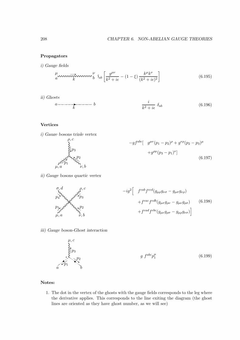
208 CHAPTER 6. NON-ABELIAN GAUGE THEORIES
Propagators
i) Gauge fields
−iδab[
gµν
k2 + iǫ− (1− ξ)
kµkν
(k2 + iǫ)2
](6.195)a b
µ ν
k
ii) Ghostsi
k2 + iǫδab (6.196)a b
k
Vertices
i) Gauge bosons triple vertex
−gfabc[ gµν(p1 − p2)ρ + gνρ(p2 − p3)
µ
+gρµ(p3 − p1)ν ]
(6.197)
µ, a ν, b
ρ, c
p1
p2
p3
ii) Gauge bosons quartic vertex
−ig2[
f eabf ecd(gµρgνσ − gµσgνρ)
+f eacf edb(gµσgρν − gµνgρσ)
+f eadf ebc(gµνgρσ − gµρgνσ)]
(6.198)
µ, a ν, b
ρ, cσ, d
p1 p2
p3p4
iii) Gauge boson-Ghost interaction
g fabcpµ1 (6.199)
µ, c
a bp1
p2
p3
Notes:
1. The dot in the vertex of the ghosts with the gauge fields corresponds to the leg wherethe derivative applies. This corresponds to the line exiting the diagram (the ghostlines are oriented as they have ghost number, as we will see)

6.2. QUANTIZATION 209
2. The other rules are as usual not forgetting the minus sign for the ghost loop becauseof their anti-commuting character.
6.2.8 Feynman rules for the interaction with matter
We have just seen the Feynman rules for the pure gauge theory, without interaction withmatter. This already non trivial due to the non-abelian character. Interaction with matteris done in the usual way, changing normal derivatives into covariant derivatives. In generalmatter is described by scalar fields, as
φi ; i = 1, ...M (6.200)
We consider also fermion fields
ψj ; j = 1, ...N (6.201)
They belong to the representations of dimension M and N , respectively. The Lagrangianwill then be
Lmatter = (Dµφ)†Dµφ−m2
φφ†φ− V (φ)
+iψDµγµψ −mψψψ
≡ Lkin + Lint . (6.202)
The interaction Lagrangian between matter and the gauge fields is easily obtainedfrom the covariant derivative
Dµij = ∂µδij − igAaµT
aij (6.203)
where T aij are the generators in the representations appropriate for the matter fields φ andψ.
We get then,
Lint = igφ∗i (∂→
− ∂←)µφjT
aijAµa + g2φ∗i T
aijT
bjkφkA
aµA
µb
+gψiγµψjT
aijA
aµ (6.204)
This leads to the following vertices:
Triple Vertices
ig(γµ)βαTaij (6.205)
µ, a
α, jβ, ip1
p2
p3

210 CHAPTER 6. NON-ABELIAN GAUGE THEORIES
ig(p1 − p2)µT aij (6.206)
µ, a
i jp1
p2
p3
Quartic Vertex
ig2gµνT a, T bij (6.207)
µ, a ν, b
i j
Group Factors
The factors fabc and T aij that appear in the Feynman rules do not need in fact to be known.In the calculations in the end will appear combinations of those that can expressed in termsof invariant quantities that characterize the group and the representation. Our generatorsare hermitian (T a† = T a) and satisfy the normalization conditions,
[T a, T b] = ifabcT c
Tr(T aT b) = δabT (R) (6.208)
In these definitions T (R) is a number that characterizes the representation R. Otherfrequently used quantity is the Casimir of the representation, defined by
∑
a,k
T aikTakj = Tr[T aT a] = δijC2(R) (6.209)
For the adjoint representation we get
facdf bcd = δabC2(G) . (6.210)
T (R) and C2(R) are not independent, they obey the relation
T (R)r = d(R)C2(R) (6.211)
where r is the dimension of the group G (number of generators) and d(R) is the dimensionof the representation R. For the adjoint representation we have
d(Adjoint) = r

6.3. WARD IDENTITIES 211
In many applications we are interested in the SU(N) family of Lie groups. For thesewe have the results
r = N2 − 1 ; d(N) = N ; d(adj) ≡ d(G) = r (6.212)
T (N) =1
2; C2(N) =
N2 − 1
2N(6.213)
T (G) = C2(G) = N (6.214)
Symmetry Factors
For the calculation of some diagrams there appear symmetry factors different from one.They were discussed before, in section5.5.5, but for completeness we recall their definitionhere. The symmetry factor is given by the # of different ways in which the lines canbe connected with the same final diagram, divided by the permutations factors for thevertices involved and by the permutation factors for the number of equal vertices.
6.3 Ward Identities
6.3.1 BRS transformation
We are now going to study the Ward identities2 for the non-abelian gauge theories. Themore convenient method is that of the Becchi, Rouet e Stora (BRS) transformations. TheBRS transformations are a generalization of the gauge transformations that make invariantthe effective action.
As we saw for non-abelian gauge theories the effective action is given by (A = gaugefield, φ = matter field)
Seff [A,φ] = S[A,φ]− 1
2ξ
∫d4xF 2
a [A,φ] −∫d4xωaMab , ω
b (6.215)
where S[A,φ] is the classical action, invariant under the (infinitesimal) gauge transforma-tions,
δAaµ = −1
gDabµ α
b
δφi = −i(T a)ijφjαa , (6.216)
and where Fa[A,φ] are the gauge conditions and the operator Mab is such that
Mabωb =
δFaδAcµ
Dcbµ ω
b +δFaδφi
ig(T b)ijφjωb . (6.217)
The efficitive action, Seff , is not invariant under gauge transformations due to the non-invariance of the gauge fixing term and of the ghost Lagrangian. This non-invariance can
2We use here the generic name of Ward identities for the more general identities for non-abelian gaugetheories, discovered by Ward, Takahashi, Slavnov and Taylor.

212 CHAPTER 6. NON-ABELIAN GAUGE THEORIES
disappear if we choose appropriate transformations for the ghosts in order to compensatethe non-invariance of
∫d4xF 2
a . These transformations, known as BRS transformations,are defined by,
δBRSAaµ = Dab
µ ωbθ
δBRSφi = ig(T b)ijφjωbθ
δBRSωa = 1
ξFa[A,φ]θ
δBRSωa = 1
2gfabcωbωcθ
(6.218)
where θ is an anti-commuting parameter independent of the space-time point (Grassmannvariable).
We see that for the fields Aaµ and φi the BRS transformations are gauge transformationswith parameter αa(x) = −gωa(x)θ. Notice the anti-commuting character of θ is necessaryfor the product ωaθ to have a bosonic (commutative) character. To show the invariance ofSeff [A,φ] we are going to prove a series of theorems needed for the general proof. Beforewe do that it is convenient to introduce the Slavnov operator, s, defined by the relations,
δBRSAaµ = sAaµθ
δBRSφi = sφiθ
δBRSωa = sωaθ
δBRSωa = sωaθ
(6.219)
This operator is distributive with respect to multiplication (like a derivative) and obeysthe following relations,
s(B1B2) = sB1B2 +B1sB2
s(F1B2) = sF1B2 + F1sB2
s(B1F2) = −sB1F2 +B1sF2
s(F1F2) = −sF1F2 + F1sF2 (6.220)
Theorem 6.3
The Slavnov operator s is nilpotent in the fields Aaµ, φi e ωa, that is s2Aaµ = s2φi =
s2ωa = 0.
Proof: We show for each case. We have
a) s2Aaµ = 0
s2Aaµ =s(Dabµ ω
b) = −δDab
µ
δAcνsAcνω
b +Dabµ sω
b
=− δνµ(−gfabc)Dcdν ω
dωb +1
2gf bcdDab
µ (ωcωd)
=
[gfabc∂µω
cωb +1
2gfacd∂µω
cωd +1
2gfacdωc∂µω
d
]
+
[gfabc(−g)f cdeAeµωdωb +
1
2g(−g)f bcdfabeAeµωcωd
]

6.3. WARD IDENTITIES 213
=(gfabc∂µωcωb − gfabc∂µω
cωb)
− 1
2g2(fabcf cde − fadcf cbe + f cdbface)Aeµω
dωb = 0 (6.221)
b) s2φi = 0
s2φi =s [ig(Ta)ijφjω
a]
=− ig(T a)ijsφjωa + ig(T a)ijφjsω
a
=g2(T a)ij(Tb)jkφkω
bωa + ig(T a)ijφj1
2gfabcωbωc
=1
2g2[T c, T b]ikω
bωcφk +i
2g2(T a)ijφjf
abcωbωc
=i
2g2(T a)ijφj(f
acb + fabc)ωbωc
=0 (6.222)
c) s2ωa = 0
s2ωa =s
(1
2gfabcωbωc
)
=− 1
2gfabcsωbωc +
1
2gfabcωbsωc
=− gfabcsωbωc
=− 1
2g2fabcf befωeωtωc
=− 1
6g2(fabcf bef + fabef bfc + fabff bce)ωeωtωc
=0 (6.223)
where we have used the anti-commutation of the ghost fields and the Jacobi identity.The theorem is then proved.
For linear gauge fixing, we can show an important result that we also give in the formof a theorem.
Theorem 6.4
For linear gauge fixings, the Slavnov operator verifies the relation
s(Mabωb) = 0 (6.224)

214 CHAPTER 6. NON-ABELIAN GAUGE THEORIES
Proof:
We saw before that
Mabωb(x) =
∫d4y
[δFa(x)
δAcµ(y)Dcbµ ω
b(y) +δFa(x)
δφi(y)ig(T b)ijφjω
b(y)
](6.225)
If we use the definitions of δBRS and of the Slavnov operator, we can write
Mabωb(x) =
∫d4y
[δFa(x)
δAcµ(y)sAcµ(y) +
δFa(x)
δφi(y)sφi(y)
]. (6.226)
If the gauge fixing is linear δFaδAcµ
and δFaδφi
do not depend on the on the fields and then
s[Mabω
b(x)]=
∫d4y
[δFa(x)
δAµ(y)s2Acµ(y) +
δFa(x)
δφi(y)s2φi(y)
]= 0 . (6.227)
where we have used the previous results. This proves the theorem.
Using theses results we can then show that the effective action is invariant under BRStransformations. We are going to show this result also in the form of a theorem.
Theorem 6.5
The action Seff is invariant under BRS transformations.
Proof:
The effective action is
Seff [A,φ] = S[A,φ] +
∫d4x
[− 1
2ξF 2a [A,φ] − ωaMabω
b
]. (6.228)
As the classical action is invariant under gauge transformations we should have
s (S[A,φ]) = 0 . (6.229)
For the other terms we have
s
(− 1
2ξF 2a − ωaMabω
b
)= −1
ξFasFa + sωaMabω
b − ωas(Mabωb) . (6.230)
But
sFa(x) =
∫d4y
[δFa
δAbµ(y)sAbµ(y) +
δFaδφi(y)
sφi(y)
]= Mabω
b(x) , (6.231)
and using one of the previous theorems we get
s(Mabωb) = 0 . (6.232)

6.3. WARD IDENTITIES 215
Therefore
s
(− 1
2ξF 2a − ωaMabω
b
)=
(−1
ξFa + sωa
)Mabω
b = 0 , (6.233)
where we have used the fact that sωa = 1ξFa. Putting everything together we get,
sSeff [A,φ] = 0 . (6.234)
For the applications we stil need another result on the invariance of the integrationmeasure that we also present as a theorem.
Theorem 6.6
The measure D(Aµ, φi, ωa, ωb) is invariant under BRS transformations.
Proof:
Simple calculations lead to the following relations
δ(sAaµ)
δAaµ= −gfabaδµµωb = 0
δ(sφi)
δφi= ig(T a)iiω
a = 0 ; (Tr(T a) = 0)
δ(sωa)
δωa= gfaacωc = 0
δ(sωa)
δωa= 0 (6.235)
As we saw in the last chapter these relations imply that the integration measure isinvariant proving the theorem
6.3.2 Ward-Takahashi-Slavnov-Taylor identities
We are now in position to derive the generalization of the Ward-Takahashi identities tonon-abelian gauge theories. This extension was done, among others, by Slavnov andTaylor, but frequently we use the short designation of Ward identities even for the non-abelian case. In a generic form Ward identities are relations among the Green functionsthat result from the gauge symmetry of the theory. As we discuss the more convenientway to describe them is through the generating functionals of the Green functions. Let usthen consider a non-abelian gauge theory. For simplicity we just consider that the matterfields are scalars φi. Fermions can be introduced later easily. The generating functional isthen
Z[Jaµ , Ji, ηa, ηa] =
∫D(Aµ, φi, ω, ω)e
i∫
d4x[Leff+JaµAµa+Jiφi+ηaωa+ωaηa ] (6.236)
where we have also introduced sources for the ghosts.
A BRS transformation is a change of variables in the integral. The value of the integralshould not be changed by this. As Seff and the measure are invariant we should have thefollowing theorem:

216 CHAPTER 6. NON-ABELIAN GAUGE THEORIES
Theorem 6.7
Given any Green function
G(x1, ..., y1, ..., z1, ..., w1, ...) = 〈0|TAaµ1(x1) · · ·φi1(y1) · · ·ωa(z1) · · ·ωb(w1) · · · |0〉(6.237)
we have the following relations:
i) s 〈0|TAaµ(x1) · · · φi1(y1) · · ·ωa(z1) · · ·ωb1(w1) |0〉 = 0
ii) 0 = 〈0|TsAaµ(x1) · · · |0〉+ · · ·+ 〈0|T · · · sφi · · · |0〉+ · · ·
+ 〈0|T · · · sωa · · · |0〉 · · · + 〈0|T · · · sωa · · · |0〉 (6.238)
Proof: The proof is clear if we write
〈0|TAaµ(x1) · · ·φi1(y1) · · ·ωa(z1) · · ·ωb(w1) |0〉 =
=
∫D(Aµ, φi, ω, ω)A
aµ(x1) · · · φi1(y1) · · ·ωa(z1) · · ·ωb(w1)e
iSeff . (6.239)
Then the BRS transformation should leave the integral invariant proving the firstrelation. Then the second relation results from the first and from the invariance ofthe measure and of the effective action.
This theorem constitutes a quick way to establish relations among Green functionsfor particular cases, as we shall see below. However to establish general results for therenormalization and gauge invariance of the S matrix, we are interested in the Wardidentities expressed in terms of the generating functionals. Using the invariance of theintegral for a change of variables, the invariance of the measure D and of Seff , we get forthe Ward identity for the generating functional Z,
0 =
∫D(Aµ, φi, ω, ω)
∫d4x(JµasAaµ + Jisφi + ηasωa − sωaηa)ei(Seff+sources) . (6.240)
The more useful Ward identities are for the functional Γ. The previous expression can notdirectly lead to Γ functional, because sAaµ, sφi and sωa are not linear in the fields. Tosolve this problem we introduce sources for these non-linear operators. We generalize theeffective action defining a new quantity Σ such that
Σ[Aaµ, φi, ωa, ωa,Ka
µ,Ki, La]
≡ Seff [Aaµ, φi, ω
a, ωa] +
∫d4x(KaµsAaµ +Kisφi + Lasωa) , (6.241)
where Kaµ,Ki and La are sources for the non-linear operators sAaµ, sφi and sω
a respec-tively. Using the previous theorems it is easy to show that Σ is invariant under BRStransformations, that is
sΣ = 0 . (6.242)
6.3. WARD IDENTITIES 217
Let us consider now the generating functional for the Green functions in the presenceof the sources Jaµ , Ji, η
a, ηa,Kµa,Ki and La, that is
Z[Jaµ , Ji, η, η,Kµ,Ki, L] =
∫D(Aµ, φi, ω, ω)e
i[Σ+
∫
d4x(JaµAµa+Jiφi+ηω+ωη)
](6.243)
We can now repeat the previous reasoning for invariance under BRS transformations. Likebefore we get (recall that sΣ = 0)
0 =
∫D(· · · )
∫d4x[Jµa sA
aµ + J isφi + ηasωa − sωaηa]ei(Σ+sources) , (6.244)
only now we have composite operators sA, sφ e sω, that is
sAaµ =δΣ
δKµa, sφi =
δΣ
δKi, sωa =
δΣ
δLa, sωa =
1
ξF a (6.245)
We get then∫
D(· · · )∫d4x
[Jµa
δΣ
δKµa+ J i
δΣ
δKi+ ηa
δΣ
δLa− 1
ξF aηa
]ei(Σ+sources) = 0 (6.246)
or in another form∫d4x
[Jµa
δ
iδKµa+ J i
δ
iδKi+ ηa
δ
iδLa− 1
ξF a[
δ
iδJµ,δ
iδJi
]ηa]eiW [Jaµ,Ji,η,η,Kµ,Ki,L] = 0
(6.247)For a linear gauge condition all the differential operators in the square bracket are of firstorder and therefore we can write
∫d4x
[Jµa
δ
δKµa+ J i
δ
δKi+ ηa
δ
δLa− 1
ξFaη
a
]W = 0 . (6.248)
This is the expression of the Ward identities for the generating functional of the con-nected Green functions, W . Normally the Ward identities are more useful for generatingfunctional of the irreducible Green functions. This defined by,
Γ[Aµ, φi, ω, ω,Kµ,Ki, L] ≡W [Jµ, Ji, η, η,Kµ,Ki, L]−∫d4x[JaµA
aµ + Jiφi + ηω + ωη]
(6.249)with the usual relations
φi = δWδJi
Aaµ = δWδJµa
ωa = δWδηa
ωa = −δWδηa
(6.250)
as usual as the inverse relations,
Ji = − δΓδφi
Jaµ = − δΓδAµa
ηa = δΓδωa
ηa = − δΓδωa
(6.251)

218 CHAPTER 6. NON-ABELIAN GAUGE THEORIES
As the Legendre transform leaves the sources Kaµ,Ki and La unchanged, we should
have.δW
δKaµ
=δΓ
δKaµ
;δW
δKi=
δΓ
δKi;
δW
δLa=
δΓ
δLa(6.252)
We then get easily∫d4x
[δΓ
δKaµ(x)
δΓ
δAµa(x)+
δΓ
δKi(x)
δΓ
δφi(x)− δΓ
δLa(x)
δΓ
δωa(x)− 1
ξF a
δΓ
δωa(x)
]= 0 (6.253)
This is the generating functional for the Ward identities for the irreducible Green func-tions. The Ward identities for specific Green functions are obtained by taking appropriatefunctional derivatives of the fields.
In the applications the previous equation is used in connection with another functionalidentity, the equation of motion (or Dyson-Schwinger) for the ghosts. This can be easilyobtained doing the following change of variables in the functional integral,
δAaµ = δφi = δωa = 0
δωa = fa = infinitesimal constant(6.254)
Then
δZ = 0 =
∫D(· · · )
(iδΣ
δωa+ iηa
)faei(Σ+sources) (6.255)
but
δΣ
δωa(x)= −Mabω
b(x) = −sFa(x)
= −∫d4y
[δFa(x)
δAbµ(y)sAbµ(y) +
δFa(x)
δφi(y)sφi(y)
]
= −∫d4y
[δFa(x)
δAbµ(y)
δΣ
δKbµ(y)+δFa(x)
δφi(y)
δΣ
δKi(y)
](6.256)
We therefore obtain
0 =
∫D(· · · )
−i∫d4y
[δFa(x)
δAbµ(y)
δΣ
δKbµ(y)+δFa(x)
δφi(y)
δΣ
δKi(y)
]+ iηa(x)
ei(Σ+sources)
=
−∫d4y
[δFa(x)
δAbµ(y)
δ
δKbµ(y)+δFa(x)
δφi(y)
δ
δKi(y)
]+ iηa(x)
eiW
(6.257)
Using now
ηa = − δΓ
δωa(6.258)
we finally get (for linear gauges)
∫d4y
[δFa(x)
δAbµ(y)
δΓ
δKµb(y)+δFa(x)
δφi(y)
δΓ
δKi(y)
]= − δΓ
δωa(x)(6.259)
which the generating functional for the Dyson-Schwinger equations for the ghosts.

6.3. WARD IDENTITIES 219
6.3.3 Example: Transversality of vacuum polarization
We are going to give an example of the application of the Ward identities. For this wewill show that the vacuum polarization is transversal. As the pure gauge theory is alreadynon-trivial, we only consider this case, the generalizations being straightforward. To showthe details of the calculations that will shed some light on the more formal expression wejust proved, we are going to do this example using two methods. The first one, that wewill call formal method, will use the general expression for the Ward identities satisfiedby the generating functional of the irreducible Green functions, Γ. The second method,which we call practical method, will use the results of one of the theorems on the BRStransformations that we proved before. The comparison between the two methods will beimportant to clarify the meaning of the expressions.
i) Formal Method
For the pure gauge theory case, the expression for the Ward identities for the generatingfunctional Γ is,
∫d4x
[δΓ
δKaµ(x)
δΓ
δAµa(x)− δΓ
δLa(x)
δΓ
δωa(x)− 1
ξF a(x)
δΓ
δωa(x)
]= 0 (6.260)
where we will choose a covariant linear gauge,
F a(x) = ∂µAaµ(x) (6.261)
To proceed it is necessary to know what is the meaning of the functional derivatives, δΓδKa
µ
and δΓδLa . From their definition we have
δΓ
δKaµ(x)
=δW
δKaµ
=δ
iδKaµ
lnZ =1
Z
δZ
iδKaµ(x)
=1
Z
∫D(· · · )sAaµ(x)ei(Σ+sources) (6.262)
As sAaµ(x) = Dabµ ω
b = ∂µωa(x)− gfabcωb(x)Acµ(x), we then get
δΓ
δKaµ(x)
= ∂xµ1
Z
δZ
iδηa(x)− gfabc
1
Z
δ2Z
iδJcµ(x)iδηb(x)
(6.263)
Introducing now Z ≡ exp(iW ), the previous expression becomes,
δΓ
δKaµ(x)
= ∂µxδ(iW )
iδηa(x)− gfabc
[δ2iW
iδJcµ(x)iδηb(x)
+δiW
iδJcµ(x)
δiW
iδηb(x)
], (6.264)
which has the following diagrammatic representation
a µµ
bb
cc
iW
iWiW
iW
δΓ
δKaµ(x)
= ∂µx −gfabc −gfabc (6.265)

220 CHAPTER 6. NON-ABELIAN GAUGE THEORIES
where W is the generating functional for the connected Green functions.
In a similar way we can show that (sωa = 12gf
abcωbωc)
δΓ
δLa(x)=
1
2g fabc
1
Z
δ2Z
iδηc(x)iδηb(x)
=1
2g fabc
[δ2(iW )
iδηc(x)iδηb(x)+
δ(iW )
iδηc(x)
δ(iW )
iδηb(x)
](6.266)
In diagrammatic form this gives
µµ
bb
cc
iW
iW
iW
δΓ
δLa(x)=
1
2g fabc +
1
2g fabc (6.267)
We want to apply δ2
δωb(y)δAcν(z)to the original equation. We get
δ2
δωb(y)δAcν(z)
(δΓ
δKaµ(x)
δΓ
δAµa(x)
)∣∣∣∣=0
=δ2Γ
δωb(y)δKaµ(x)
∣∣∣∣=0
δ2Γ
δAcν(z)δAµa(x)
∣∣∣∣=0
(6.268)
But we have
δ2Γ
δωb(y)δKaµ(x)
∣∣∣∣=0
=
∫d4w
(−i δ2Γ
δωb(y)δωf (w)
) (δ2Γ
iδηf (w)δKaµ(x)
)∣∣∣∣=0
= ∂µx
∫d4w
(−i δ2Γ
δωb(y)δωf (w)
) (δ2(iW )
iδηf (w)iδηa(x)
)∣∣∣∣=0
− g fab′c
∫d4w
(−i δ2Γ
δωb(y)δωf (w)
) (δ3iW
iδηf (w)iδηb′(x)iδJcµ(x)
)∣∣∣∣∣=0
= ∂µx δ4(x− y)δab − gfab
′c
∫d4w
(−i δ2Γ
δωb(y)δωf (w)
)
(δ3iW
iδηf (w)iδηb′(x)iδJcµ(x)
)∣∣∣∣∣=0
(6.269)
In a similar way we have for the second term,
δ2
δωb(y)δAcν(z)
(δΓ
δLaδΓ
δωa
)∣∣∣∣=0
= 0 (6.270)
δ2
δωb(y)δAcν(z)
(1
ξ∂ρA
ρa(x)δΓ
δωa(x)
)∣∣∣∣=0
=1
ξ∂νxδ
4(x− z)δ2Γ
δωb(y)δωa(x)
∣∣∣∣=0
(6.271)
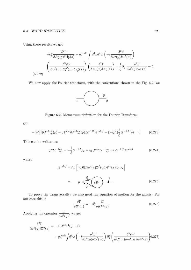
6.3. WARD IDENTITIES 221
Using these results we get
−∂yµδ2Γ
δAbµ(y)δAcν(z)
− gfade∫d4xd4w
(−i δ2Γ
δωb(y)δωf (w)
)
(δ3iW
iδηf (w)iδηd(x)iδJeµ(x)
)(δ2Γ
δAaµ(x)δAcν(z)
)+
1
ξ∂νz
δ2Γ
δωb(y)δωc(z)= 0
(6.272)
We now apply the Fourier transform, with the conventions shown in the Fig. 6.2, we
p
z y
Figure 6.2: Momentum definition for the Fourier Transform.
get
−ipµ(i)G−1cbνµ(p)− gfadeiG−1caνµ(p)∆−1fbXµdef + (−ipν) i
ξ∆−1cb(p) = 0 (6.273)
This can be written as
pµG−1cbνµ = −1
ξ∆−1cbpν + ig fadeG−1caνµ(p) ∆
−1fbXµdef (6.274)
where
Xµdef =FT[< 0|Tωd(x)ωf (w)Aµe(x)|0 >c
]
≡ (6.275)µ
d
e
fiW
To prove the Transversality we also need the equation of motion for the ghosts. Forour case this is
δΓ
δωa(z)= −∂µz
δΓ
δKµa(z)(6.276)
Applying the operator δδωb(y)
, we get
δ2Γ
δωb(y)δωa(z)=− ⊔⊓ δabδ4(y − z)
+ gfadc∫d4w
(−i δ2Γ
δωb(y)δωf (w)
)∂µz
(δ3iW
iδJcµ(z)iδηf (w)iδηd(z)
)(6.277)

222 CHAPTER 6. NON-ABELIAN GAUGE THEORIES
Applying now the Fourier transform, we get
i∆−1ab = p2δab + gfadc(−ipµ)Xdcfµ ∆−1fb (6.278)
The previous equations allow now to complete the proof of the transversality of thevacuum polarization. For this we write,
G−1abµν = G−1Tabµν + i
a
ξδabpµpν (6.279)
where pµG−1Tabµν = 0. For the free propagator we have a = 1. to show the transversality
we just have to show that the longitudinal part is not renormalized and that therefore thevalue of a remains always a = 1. Using
pµG−1abµν = ia
ξδabp2pν (6.280)
and multiplying equation by pν we obtain
ia
ξp4δcb = −1
ξp2∆−1cb − a
ξp2g f cdepµX
µdef∆−1fb (6.281)
Using now equation Eq. (6.278) we get after some trivial algebra
0 = −1
ξp2∆−1cb +
a
ξp2∆−1cb (6.282)
This implies
a = 1 (6.283)
as we wanted to shown.
2) Practical Method
Now we are going to use the so-called practical method based in Theorem 6.7 Using
sωb(x) =1
ξ∂µA
µb(x) (6.284)
and
sAaν = ∂νωa − gfadcωdAcν (6.285)
it is easy to see that the starting Green function should be⟨0|TAaν(x)ωb(y)|0
⟩. Then
Theorem 6.7 tells us that
s⟨0|TAaµ(x)ωb(y)|0
⟩= 0 (6.286)
that is
1
ξ
⟨0|TAaν(x)∂µAµb(y)|0
⟩=
⟨0|T∂νωa(x)ωb(y)|0
⟩
−gfadc⟨0|Tωd(x)Acν(x)ωb(y)|0
⟩(6.287)

6.3. WARD IDENTITIES 223
We now take the Fourier transform obtaining
i
ξpρGabνρ(p) = −ipν∆ab(p)− gfadcXdcb
ν (6.288)
where Xdcbν has been defined before. Multiplying by G−1νµ∆−1 we then get
pµG−1acνµ = −1
ξpν∆
−1ac + igf fdeχdebν ∆−1bcG−iνµaf (6.289)
which is precisely Eq. (6.274) The result in Eq. (6.278) can be easily obtained knowingthat the only vertex of the ghosts is
gfabcpµ (6.290)
µ, c
a b
p
Then
µ
daa abb b
cp
iW iW= + (6.291)
which means
∆ab(p) =i
p2δab +
i
p2gfadcpµXdcb
µ (6.292)
or in another formi∆−1ab = p2δab − igfadcpµXdcb′
µ ∆−1b′b (6.293)
which is precisely Eq. (6.278). The proof of transversality follows now the same steps asin the formal case.
6.3.4 Gauge invariance of the S matrix
We have shown before the gauge invariance of the S matrix using the equivalence theoremand the fact that the generating functionals corresponding to different gauge conditionsonly differ in the source terms. The proof used some properties of the Coulomb gauge andthis can raise some doubts about the genera validity of the argument.
We are going to show here, using the Ward identities, that the functionals ZF andZF+∆F corresponding to the gauge conditions F and F +∆F , respectively, only differ inthe source terms. As F and ∆F are arbitrary th proof is general. We have
ZF [Jaµ , Ji] =
∫D(· · · )ei[Seff+
∫
d4x(JaµAµa+Jiφi)] (6.294)

224 CHAPTER 6. NON-ABELIAN GAUGE THEORIES
Then
ZF+∆F − ZF =
∫D(· · · )
∫d4x i
[−1
ξF a∆F a − ωa
∫d4y
δ∆F a(x)
δAbµ(y)sAbµ(y)
−ωa∫d4y
δ∆F a(x)
δφi(y)sφi(y)
]ei(Seff+sources) (6.295)
We use now the Ward identities in the form that corresponds to the generating functionalZ, that is
0 =
∫D(· · · )
∫d4x[JµasAaµ + J isφi + ηsω − sωη] ei(Seff+J
aµA
µa+Jiφi+ωη+ηω) (6.296)
Taking the derivative in order to ηa(x) and setting after the ghost sources to zero, we get
0 =
∫D(· · · )
[1
ξF a(x) + iωa(x)
∫d4y[JµbsAbµ + J isφi]
]ei[Seff+
∫
d4x(JaµAµi+Jiφi)] (6.297)
or
−1ξF a[δiδJ
] ∫D(· · · )ei(Seff+sources) =
=
∫D(· · · )iωa(x)
∫d4y[JµbsAbµ + Jisφi]e
i(Seff+sources)
(6.298)
Then
∫D(· · · )
(−1ξF a∆F a
)ei(Seff+sources) =
= ∆F a[δiδJ
] (−1ξF a[δiδJ
])∫D(· · · )ei(Seff+sources)
= ∆F a[δiδJ
] ∫D(· · · )iωa(x)
∫d4y[JµbsAbµ + J isφi]e
i(Seff+sources)
=
∫D(· · · )
ωa(x)
∫d4y
[δ∆F a(x)
δAbµ(y)sAbµ(y) +
δ∆F a(x)
δφi(y)sφi(y)
]
+iωa(x)∆F a(x)
∫d4y[JµbsAbµ + J isφi]
ei(Seff+sources)
(6.299)
We get therefore
∫D(· · · )
(−1
ξF a∆F a−ωa(x)
∫d4y
[δ∆F a(x)
δAbµ(y)sAbµ(η)+
δ∆F a
δφi(y)sφi(y)
])ei(Seff+sources)
=
∫D(· · · )iωa(x)∆F a(x)
∫d4y
[JµbsAbµ + J isφi
]ei(Seff+sources)
(6.300)

6.4. WARD TAKAHASHI IDENTITIES IN QED 225
We can then write
ZF+∆F −ZF
=
∫D(· · · )i
∫d4x[iωa(x)∆F a(x)
∫d4y(JµbsAbµ + Jisφi)
]ei(Seff+sources)
=
∫D(· · · )e
iSeff+
∫d4y[Jaµ(y)Aµa(y) + JiΦi(y)]
(6.301)where
Φi(y) ≡ φi(y) + i
∫d4x[ωa(x)∆F a(x)sφi(y)] (6.302)
and
Aaµ(y) ≡ Aaµ(y) + i
∫d4x[ωb(x)∆F b(x)sAaµ(y)] (6.303)
The difference between the generating functionals ZF+∆F and ZF is only in the functionalform of the source terms. We can then use the equivalence theorem to show that therenormalized S matrix are equal in both cases.
SRF+∆F = SRF . (6.304)
6.4 Ward Takahashi Identities in QED
6.4.1 Ward-Takahashi identities for the functional Z[J ]
We will now derive again the Ward identities for QED, that we found in our study ofrenormalization, using now the functional methods. The generating functional for theGreen functions for QED is given by, in a linear gauge,
Z(Jµ, η, η) =
∫D(Aµ, ψ, ψ)e
i(Seff+∫
d4x(JµAµ+ηψ+ψη) (6.305)
where Jµ, η e η are the sources for Aµ, ψ and ψ respectively. The effective action is givenby,
Seff =
∫d4x
[LQED − 1
2ξ(∂ ·A)2
]= SQED + SGF (6.306)
where
LQED = −1
4FµνF
µν + ψ(iγµDµ −m)ψ . (6.307)
SQED is invariant under local gauge transformation of the group U(1) that we write as,
δAµ = ∂µΛ
δψ = −ieΛψδψ = ieΛψ

226 CHAPTER 6. NON-ABELIAN GAUGE THEORIES
The Seff contains the part of the gauge fixing that it is not invariant under these trans-formations. Therefore the Ward identities take the form,
(δSGFδφi
[δ
iδJ
]+ Ji
)Fi
[δ
iδJ
]Z(J) = 0 (6.308)
This can be written in our case as, putting back the explicit integrations,
0 =
∫d4x
[1
ξ∂µ∂ν
(δ
iδJν
)∂µΛ+ Jµ∂µΛ− ieΛη
δ
iδη+ ieΛη
δ
iδη
]Z(Jµ, η, η) (6.309)
After an integration by parts we get,∫d4x Λ
[−1
ξ⊔⊓∂ν
(δ
iδJν
)− ∂µJ
µ − ieηδ
iδη+ ieη
δ
iδη
]Z(Jµ, η, η) = 0 (6.310)
This can be written as[1
ξ⊔⊓∂µ
(δ
iδJµ
)+ ∂µJ
µ + ieη
(δ
iδη
)− ieη
(δ
iδη
)]Z(J, η, η) = 0 (6.311)
6.4.2 Ward-Takahashi identities for the functionals W and Γ
From the point of view of the applications it is more useful the Ward identity for thegenerating functional of the irreducible Green functions. This problem is simpler than inthe case of non-abelian gauge theories, that we just discuss, as the the previous equationis linear in the functional derivatives with respect to the different sources (we notice thatif we had chosen a non-linear gauge fixing this would not be true, even in QED). Thelinearity allow us to write immediately
∂µJµ +
[1
ξ⊔⊓∂µ
(δ
iδJµ
)+ ieη
δ
iδη− ieη
δ
iδη
]W (J, η, η) = 0 (6.312)
where W is the generating functional for the connected Green functions,
Z(Jµ, η, η) ≡ eiW (Jµ,η,η) (6.313)
As we saw the generating functional for the irreducible Green functions is given by,
Γ(Aµ, ψ, ψ) =W (Jµ, η, η)−∫d4x[JµAµ + ηψ + ψη] (6.314)
We also have the relations
Aµ =δW
iδJµ; ψ =
δW
iδη; ψ = −δW
iδη(6.315)
and
Jµ = − δΓ
δAµ; η = − δΓ
δψ; η =
δΓ
δψ(6.316)
where, as usual, the fermionic derivatives are left derivatives. We can them write
1
ξ⊔⊓∂µAµ − ∂µ
δΓ
δAµ+ ie
δΓ
δψψ + ieψ
δΓ
δψ= 0 (6.317)
This equation is the starting point to generate all the Ward identities in QED. Its applica-tion it is much easier than the equivalent expression that was proved using the canonicalformalism. The functional methods make this expressions particularly simple.

6.4. WARD TAKAHASHI IDENTITIES IN QED 227
6.4.3 Example: Ward identity for the QED vertex
To convince ourselves that this equation reproduces the Ward identities that we already
know, let us derive the Ward identity for the vertex in QED. We applyδ2
δψα(y)δψβ(z)to
the master equation. We get then
∂µxδ3Γ
δψα(y)δψβ(z)δAµ(x)
=ie
[δ2Γ
δψα(y)δψβ(x)δ4(z − x)− δ2Γ
δψα(x)δψβ(z)δ4(y − x)
](6.318)
This equation means
∂µxΓµβα(x, z, y) = ie[Γβα(x, y)δ
4(z − x)− Γβα(z, x)δ4(y − x)
](6.319)
Taking now the Fourier transform to both sides of the equation, with the momentadefined as the Fig. 6.3, we get,
µ
β α
pp′
q = p′ − p
Figure 6.3: Definition of the momenta for the vertex.
qµΓµ(p′, p) = ie[S−1(p)− S−1(p′)] (6.320)
This is precisely the well known Ward identity.
6.4.4 Ghosts in QED
We said before that the generating functional for QED was given by,
Z(Jµ, η, η) =
∫D(Aµ, ψ, ψ)e
i∫
d4x[LQED+LGF+JµAµ+ηψ+ψη] (6.321)
where LQED is the usual Lagrangian for QED and the gauge fixing term was,
LGF = − 1
2ξ(∂ ·A)2 . (6.322)
228 CHAPTER 6. NON-ABELIAN GAUGE THEORIES
In fact this is not strictly true. If we use the prescription for the gauge theories, we wouldget instead,
Z(Jµ, η, η, ζ, ζ) =
∫D(Aµ, ψ, ψ, ω, ω)e
i∫
d4x[Leff+JµAµ+ηψ+ψη+ωζ+ζω] (6.323)
In this expression ω e ω are anti-commuting scalar fields known as the Faddeev-Popovghosts as we saw before. Although in physical process they never appear as external states,it is useful to introduce also sources for them to discuss the Ward identities.
In the previous action, the Lagrangian Leff is
Leff = LQED + LGF + LG (6.324)
where LG = −ω ⊔⊓ ω (6.325)
The reason why in QED we can work with the functional Z instead of Z is because theghosts do not have interactions with the gauge fields and can be integrated out (Gaussianintegration) and absorbed in the normalization. Nevertheless, for the Ward identitiesit is useful to keep them. The effective Lagrangian, Leff , is invariant under the BRStransformations given by,
δψ = −ieωθψδψ = ieψωθ
δAµ = ∂µωθ
δω = 1ξ (∂ · A)θ
δω = 0
(6.326)
The parameter θ is an anti-commuting (Grassmann variable). The BRS transformationson the physical fields are gauge transformations with parameter Λ = ωθ and thereforeLQED is left invariant. The transformations in the ghosts ω and ω are such that thevariation of LGF cancels that of LG, just like in the non-abelian case. The invariance ofthe integration measure and of Seff allows us to write immediately the Ward identitiesfor the generating functionals. The BRS transformations allow us to obtain the Wardidentities in a quick way without having to resort to the functional Γ. This method isbased on the fact, as we saw in Theorem refth:Slavnov, that the application of the operatorδBRS to any Green function gives zero, that is
δBRS 〈0|TAµ1 · · ·ω · · ·ω · · ·ψ · · ·ψ · · · |0〉 = 0 (6.327)
Let us show two simple applications of the method in QED.
1) The non-renormalization of the longitudinal photon propagator
This result is equivalent, as we have seen, to the statement that the vacuum polarizationis transversal. It is proved easily starting with the Green function, 〈0|TAµω |0〉, and using
δBRS 〈0|TAµω |0〉 = 0 (6.328)
This gives1
ξ〈0| |TAµ∂νAν |0〉 θ − 〈0|T∂µωω |0〉 θ = 0 (6.329)
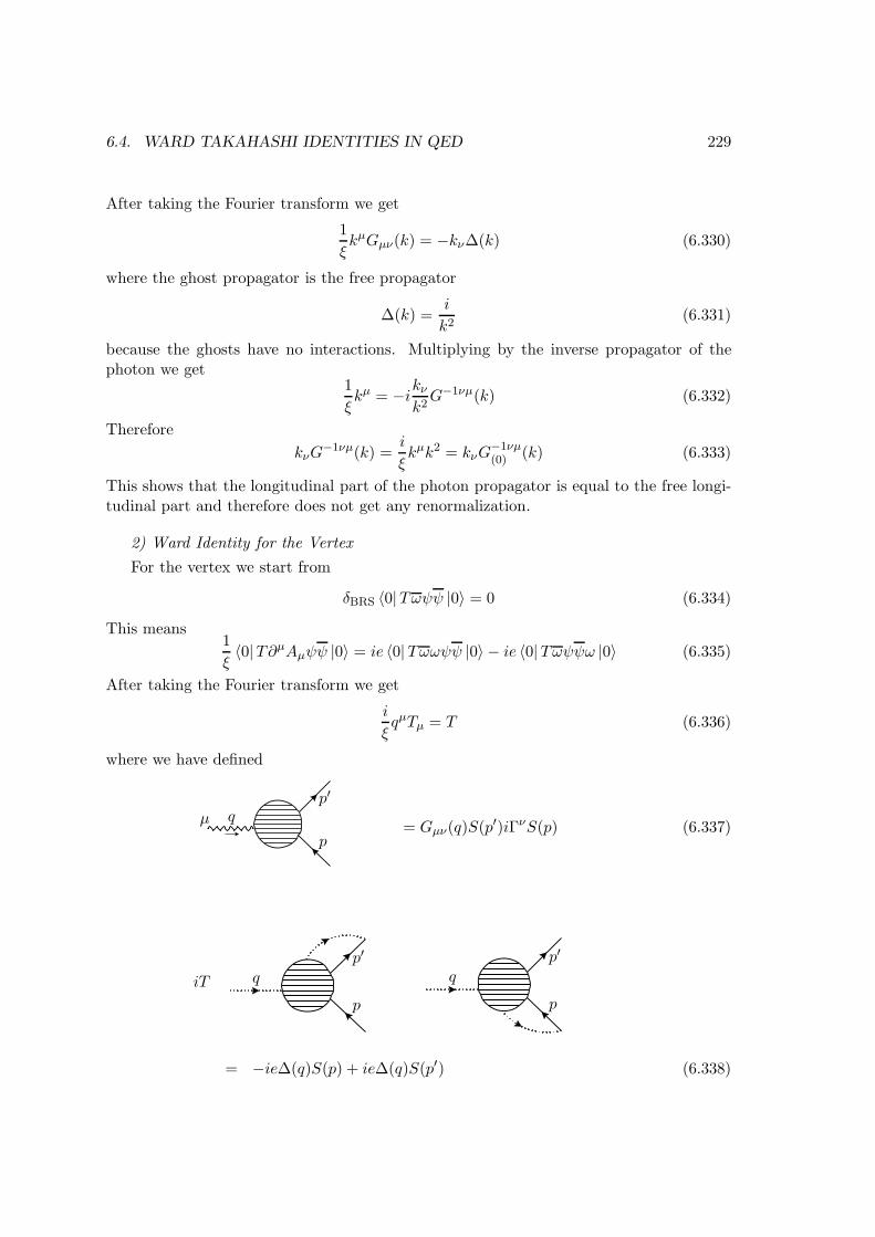
6.4. WARD TAKAHASHI IDENTITIES IN QED 229
After taking the Fourier transform we get
1
ξkµGµν(k) = −kν∆(k) (6.330)
where the ghost propagator is the free propagator
∆(k) =i
k2(6.331)
because the ghosts have no interactions. Multiplying by the inverse propagator of thephoton we get
1
ξkµ = −ikν
k2G−1νµ(k) (6.332)
Therefore
kνG−1νµ(k) =
i
ξkµk2 = kνG
−1νµ(0) (k) (6.333)
This shows that the longitudinal part of the photon propagator is equal to the free longi-tudinal part and therefore does not get any renormalization.
2) Ward Identity for the Vertex
For the vertex we start from
δBRS 〈0|Tωψψ |0〉 = 0 (6.334)
This means1
ξ〈0|T∂µAµψψ |0〉 = ie 〈0|Tωωψψ |0〉 − ie 〈0|Tωψψω |0〉 (6.335)
After taking the Fourier transform we get
i
ξqµTµ = T (6.336)
where we have defined
iTµ = = Gµν(q)S(p′)iΓνS(p) (6.337)
µ
p
qp′
iT = −ie + ie
= −ie∆(q)S(p) + ie∆(q)S(p′) (6.338)
p
qp′
p
qp′

230 CHAPTER 6. NON-ABELIAN GAUGE THEORIES
The last equality results from the fact that ghosts have no interactions in QED in alinear gauge. Putting everything together we get
i
ξqµGµν(q)S(p
′)iΓνS(p) = −ie∆(q)S(p) + ie∆(q)S(p′) (6.339)
Using1
ξkµGµν(k) = −kν∆(k) (6.340)
and multiplying by the inverse of the fermion propagators we get again the well knownthe Ward identity for the vertex,
qµΓµ(p′, p) = ie
[S−1(p)− S−1(p′)
](6.341)
6.5 Unitarity and Ward Identities
6.5.1 Optical Theorem
The S matrix, (Heisenberg 1942), can be written in the form
S = 1 + iT (6.342)
Then its unitarity SS† = 1 implies,
2 ImT = TT † (6.343)
If we insert this relation between the same initial and final state (elastic scattering) weget
2 Im 〈i|T |i〉 =⟨i|TT †|i
⟩
=∑
f
| 〈f |T |i〉 |2 (6.344)
where we have introduced a complete set of states. This relation can still be written inthe form,
σtotal = 2 Im T elasticforward (6.345)
known as the optical theorem. What we call here σtotal it is not exactly the cross section,because the flux factors are mixing. It is for our purpose the quantity defined by
σtotal ≡∑
f
| 〈f |T |i〉 |2 (6.346)
Unitarity establishes therefore a relation between the total cross section and the imag-inary part of the elastic amplitude in the forward direction (the initial and final state haveto be the same).
6.5. UNITARITY AND WARD IDENTITIES 231
6.5.2 Cutkosky rules
To show that unitarity is obeyed in a given process we have to know how to calculate theimaginary part of Feynman diagrams. Of course there is always the possibility of doingexplicitly the calculations and retrieve the imaginary part, but this only possible for simplediagrams (see below). Therefore it is useful to have rules, known as Cutkosky rules, thatgive us the imaginary part of any diagram. We will state them now.
Rule 1
The imaginary part of an amplitude is obtained using the expression
2 Im T = −∑
cuts
T (6.347)
Rule 2
The cut is obtained by writing the amplitude iT = · · · and substituting in this expressionthe propagators of the lines we cut by the following expression,
• Scalar fields
∆(p) ⇒ 2πθ(po)δ(p2 −m2) (6.348)
• Fermion fields
S(p) ⇒ (p/+m)2πθ(po)δ(p2 −m2) (6.349)
• Vector gauge fields (in the Feynman gauge)
Gµν(p) ⇒ −gµν2πθ(p0)δ(p2 −m2) (6.350)
In these expression the θ functions ensure the energy flux. The Cutkosky rules arecomplicated to prove in general (see G. ’t Hooft, ”Diagrammar”, CERN Report 1972) butwe are going to show in the two explicit examples how they work.
Example 6.1 Free propagator
For the free propagator of a scalar field the amplitude is
iT =i
p2 −m2 + iε(6.351)
The imaginary part is obtained using
1
x+ iε= P
(1
x
)− iπδ(x) (6.352)
Therefore
T = P
(1
p2 −m2
)− iπδ(p2 −m2) (6.353)

232 CHAPTER 6. NON-ABELIAN GAUGE THEORIES
The imaginary part is then
2 ImT = −2πδ(p2 −m2) (6.354)
Using the Cutkosky rule we get
2 ImT = −2πδ(p2 −m2)θ(p0) (6.355)
which is precisely the same result. The function θ(p0) tell us that the flux of energyis from left to right.
Example 6.2 Self-energy in φ3
Let us consider the self-energy in the theory given by the Lagrangian,
L =1
2∂µφ∂
µφ− 1
2m2φ2 − λ
3!φ3 (6.356)
The self-energy is given by the diagram in the Fig. 6.4. The corresponding amplitude
p
kk
p− k
Figure 6.4: Self-energy
is
iT = (−iλ)2∫
d4p
(2π)4i
p2 −m2 + iε
i
(p− k)2 −m2 + iε(6.357)
Let us calculate the imaginary part of T by two methods, first doing the explicitcalculation and second using the Cutkosky rule.
i) Explicit Calculation
iT =λ2∫
d4p
(2π)41
(p2 −m2 + iε)[(p − k)2 −m2 + iε]
=λ2∫
d4p
(2π)4
∫ 1
0dx
1
(p2 + 2p · P −M2 + iε)2
=λ2∫
d4p
(2π)4
∫ 1
0dx
1
[(p + P )2 −∆]2(6.358)
where P = −x k∆ = P 2 +M2 = m2 − k2x(1− x)− iε
(6.359)

6.5. UNITARITY AND WARD IDENTITIES 233
The amplitude is then
iT = λ2∫
d4p
(2π)4
∫ 1
0dx
1
(p2 −∆)2(6.360)
The integral is divergent. Using dimensional regularization we get
T =λ
16π2µεΓ
(2− d
2
)∫ 1
0dx∆−(2−
d2) (6.361)
Choosing on-shell renormalization, TR(k2 = m2) = 0, we get
TR =T − T (k2 = m2)
=λ2
16π2Γ(ε2
)∫ 1
0dx
[(∆(k2)
µ2
)− ε2
−(∆(k2 = m2)
µ2
)− ε2
]
=λ2
16π2
(2
ε− C +O(ε)
)∫ 1
0dx
[1− 1− ε
2lnm2 − k2x(1− x)− iε
m2 −m2x(1− x)− iε
]
=− λ2
16π2
∫ 1
0dx ln
[1− βx(1− x)− iε
1− x(1− x)− iε
]= − λ2
16π2[L(β)− L(1)] (6.362)
In this expression β = k2
m2 and the function L(β) is given by
L(β) ≡∫ 1
0dx ln
[1− β(1− x)x− iε
](6.363)
It satisfies
ImL(β) = −π√1− 4
βθ(β − 4) (6.364)
Therefore
ImT = − λ2
16π2[ImL(β)− ImL(1)
](6.365)
and we get finally,
ImT =λ2
16π
√1− 4m2
k2θ
(1− 4m2
k2
)(6.366)
The θ functions ensures that there is only imaginary part when the intermediatestate could also be a final state (production of two particles of mass m).
ii) Using the Cutkosky rules
Using the rules we get
2ImT =− (iλ)2∫
d4p
(2π)4(2π)2θ(p0)θ(k0 − p0)δ(p2 −m2)δ((p2 − k2)−m2)
=λ2∫
d4p
(2π)4d4p′(2π)2θ(p0)θ(k0 − p0)δ(p2 −m2)δ(p′2 −m2)δ4(p′ − k + p)

234 CHAPTER 6. NON-ABELIAN GAUGE THEORIES
(6.367)
Using now the result∫d4p θ(p0)δ(p2 −m2) =
∫d3p
1
2p0(6.368)
We get
2ImT = λ2∫
d3p
(2π)3d3p′
1
2p01
2p′02πδ4(p′ − k + p) (6.369)
or
2ImT = λ2∫
d3p
(2π)31
2p01
2p′02πδ(k0 − p0 − p′0) (6.370)
k = (√s,~0) ; p = (
√|~p|2 +m2, ~p) ; p′ = (
√|~p′|2 +m2,−~p) (6.371)
Therefore we get
2ImT =λ2∫
d3p
(2π)31
4(|~p|2 +m2)2πδ(
√s− 2
√|~p|2 +m2)
=λ2
4π
∫d|~p| |~p|2
|~p|2 +m2
δ(|~p| −√
s4 −m2)
2|~p|√|~p|2+m2
θ
(1− 4m2
s
)
=λ2
8π
√1− 4m2
sθ
(1− 4m2
s
)(6.372)
Using s = k2 we get
ImT =λ2
16π
√1− 4m2
k2θ
(1− 4m2
k2
)(6.373)
which is the same result as we got in the explicit calculation.
6.5.3 Example of Unitarity: scalars and fermions
As an example of checking the unitarity let us consider a theory described by the La-grangian,
L = iψ∂/ψ −mψψ +1
2∂µφ∂
µφ− 1
2M2φ2 + gψψφ (6.374)
We will show unitarity in two cases (cutting fermions lines):
i) Scalar Self-energy
The self-energy of the scalars is given by the diagram in Fig. 6.5, to which correspondsthe amplitude,
iT = g2∫
d4p
(2π)4Tr
[i
p/−m+ iε
i
p/− k/−m+ iε
](6.375)

6.5. UNITARITY AND WARD IDENTITIES 235
p
kk
p− k
Figure 6.5: Fermion contribution to the scalar self-energy.
Applying Cutkosky rules we get,
2 ImT =−∑
cuts
T
=− g2∫
d4p
(2π)4Tr[(p/+m)(p/− k/+m)](2π)θ(p0)δ(p2 −m2)
(2π)θ(k0 − p0)δ((p − k)2 −m2) (6.376)
To show the unitarity we calculate the cross section,
σ =∑
f
∣∣∣∣∣∣∣∣∣∣
∣∣∣∣∣∣∣∣∣∣
2
(6.377)k
p
p′
We get
σ =∑
f
|igu(p)v(p′)|2 = −g2∑
f
Tr[(p/+m)(−p/′ +m)] (6.378)
where we have used∑
spins v(p′)v(p) = −(−p/′+m) and
∑spins u(p)u(p
′) = p/+m. Therefore
σ = −g2∫dρ2Tr[(p/+m)(−p/′ +m)] (6.379)
where dρ2 is the phase space of two particles, that is,∫dρ2 ≡
∫d3p
(2π)3d3p′
(2π)31
2p01
2p′0(2π)4δ4(k − p− p′)
=
∫d4p
(2π)4d4p′
(2π)4(2π)θ(p0)δ(p2 −m2)(2π)θ(p′0)δ(p′2 −m2)(2π)4δ4(k−p−p′)
(6.380)We conclude then that
σ =− g2∫
d4p
(2π)4(2π)θ(p0)δ(p2 −m2)(2π)θ(k0 − p0)δ((p − k)2 −m2)
Tr[(p/+m)(p/− k/+m)] (6.381)
Comparing we obtain2ImT = σ (6.382)

236 CHAPTER 6. NON-ABELIAN GAUGE THEORIES
ii) General case
Let us consider the general case of two internal fermion lines. The amplitude iT is repre-sented by the diagram
k1k1
k2k2
knkn
p
−p′≡ iT
p′ =n∑
i=1
ki − p (6.383)
The amplitude iT is given by
iT = −∫
d4p
(2π)4Tr[T ′S(p)T ′S(−p′)
](6.384)
Where we have defined the amplitude iT ′ by
≡ u(p)iT ′v(p′) (6.385)
k1
k2
kn
p
−p′
Therefore
2 ImT =−∫
d4p
(2π)4(2π)2δ(p2 −m2)θ(p0)δ(p′2 −m2)θ(p′0)
Tr[T ′(p/+m)T ′(−p/′ +m)
]
=−∫dρ2Tr
[T ′(p/+m)T ′(−p/′ +m)
](6.386)
On the other hand

6.5. UNITARITY AND WARD IDENTITIES 237
σ =∑
f
∣∣∣∣∣∣∣∣∣∣∣∣∣∣∣∣∣
∣∣∣∣∣∣∣∣∣∣∣∣∣∣∣∣∣
2
=∑
f
|u(p)T ′v(p′)|2
= −∫dρ2Tr
[(p/+m)T ′(−p/′ +m)T ′
](6.387)
k1
k2
kn
p
−p′
Therefore
σ = 2ImT (6.388)
If the lines to be cut were scalars the result would be the same. In this case there willbe no minus sign from the loop but there will be no minus sign from the spins sum. Theproof is left as an exercise.
k1k1 k1k2k2 k2
knkn kn
p p
−p′ −p′2 Im =
∑
f
∣∣∣∣∣∣∣∣∣∣∣∣∣
∣∣∣∣∣∣∣∣∣∣∣∣∣
2
(6.389)
6.5.4 Unitarity and gauge fields
In the previous slides we have shown that unitarity holds for theories with scalar andfermion fields. We are now going to show that the proof of unitarity for gauge theoriesis more complicated and requires the use of the ward identities. The problem residesin the fact that the gauge fields in internal lines have unphysical polarizations while thefinal states should have only physical degrees of freedom. This difference would lead toa violation of unitarity in gauge theories. However we will show that the ghosts in theinternal lines will compensate for the this and will make the theory unitary as it should.Let us define the following amplitudes

238 CHAPTER 6. NON-ABELIAN GAUGE THEORIES
iT =
iT abµν =
iT ab = (6.390)
+
k1k1
k2k2
p1p1p1p1
p2p2p2p2
k1
k2
p1
p2
µ, a
ν, b
k1
k2
p1
p2
a
b
wherek2 = p1 + p2 − k1 (6.391)
Using these definitions we can write the amplitude in the form (the factor 1/2 is asymmetry factor for the gauge fields and the minus sign is for the loop of ghosts)
iT =
∫d4k1(2π)4
1
2T abµνG
aa′
µµ′(k1)Gbb′
νν′(k2)T∗a′b′µ′ν′ − T ab∆aa′(k1)∆
bb′(k2)T∗a′b′
(6.392)
Applying the Cutkosky rules we find for the imaginary part
2 ImT =
∫d4k1(2π)4
(2π)2θ(k01)θ(k02)δ(k
21)δ(k
22)
1
2T abµνT
∗abµν − T abT ∗ab
≡∫dρ2
[1
2T abµνT
∗abµν − T abT ∗ab]
(6.393)
Now we have to evaluate σtotal. As the ghosts are not physical we have
σ =∑
∣∣∣∣∣∣∣∣∣∣∣
∣∣∣∣∣∣∣∣∣∣∣
2
=1
2
∫dρ2
∑
Pol
∣∣∣εµ(k1)εν(k2)T abµν∣∣∣2
(6.394)
k1
k2
p1
p2
µ, a
ν, b

6.5. UNITARITY AND WARD IDENTITIES 239
where the factor 1/2 comes now from identical particles in the final state. Writing
∑
Pol
εµ(k1)εµ′∗(k1) = Pµµ
′
(k1) (6.395)
we get
σ =
∫dρ2
1
2T abµνT
∗abµ′ν′P
µµ′(k1)Pνν′(k2) (6.396)
We now use the result (see problems)
Pµν(k) = −gµν + kµην + kνηµ
k · η (6.397)
where ηµ is a four-vector that satisfies η · ε and η2 = 0. We get
1
2T abµνT
∗abµ′ν′P
µµ′(k1)Pνν′(k2) =
=1
2T abµνT
∗abµν − 1
2(T ab · k2) · (T ∗ab · η)
1
k2 · η
− 1
2(T ab · η) · (T ∗ab · k2)
1
k2 · η− 1
2(k1 · T ab) · (η · T ∗ab)
1
k1 · η
− 1
2(η · T ab) · (k1 · T ∗ab)
1
k1 · η+
[1
2(k1 · T ab · η)(η · T ∗ab · k2)+
+1
2(k1 · T ab · k2)(η · T ∗ab · η) +
1
2(η · T ab · η)(k1T ∗ab · k2)
+1
2(η · T ab · k2)(k1 · T ∗ab · η)
]1
(k1 · η)(k2 · η)(6.398)
Using the following Ward identities (see problems),
kµ1Tabµν = k2νT
ab
kµ2Tabµν = k1νT
ab=⇒ k1 · T ab · k2 = 0 (6.399)
we get
1
2T abµνT
∗abµ′ν′P
µµ′(k1)Pνν′(k2) =
=1
2T abµνT
∗abµν − 1
2T ab(k1 · T ∗ab · η)
1
k2 · η
− 1
2T ∗ab(k1 · T ab · η)
1
k2 · η− 1
2T ab(η · T ∗ab · k2)
1
k1 · η
− 1
2(η · T ab · k2)T ∗ab
1
k1 · η+
1
2T abT ∗ab +
1
2T abT ∗ab
=1
2T abµνT
∗abµν − T abT ∗ab (6.400)

240 CHAPTER 6. NON-ABELIAN GAUGE THEORIES
Therefore after the sum over polarizations is correctly taken in account we obtain,
σ =
∫dρ2
[1
2T abµνT
∗abµν − T abT ∗ab]
(6.401)
Comparing with the expression for 2 ImT we get
σ = 2 ImT (6.402)
as we wanted to show.
It should be clear that the ghosts with their minus sign of the loop played a crucialrole in subtracting the extra degrees of freedom. Also the Ward identities were necessaryto relate the gauge field amplitudes with the ghost amplitude.

Problems 241
Problems for Chapter 6
2.1 Mostre que T (R) esta relacionado com o operador de Casimir da representacao RC2(R) atraves de
T (R)r = d(R)C2(R) (6.403)
onde r e a dimensao do Grupo G e d(R) e a dimensao da representacao R. O CasimirC2(R) e definido por
∑
a,k
T aikTakj = δij ...C2(R) . (6.404)
2.2 Mostrar que numa escolha diferente de condicoes auxiliares χiα = 0 conduz ao mesmoresultado.
Sugestao: considere uma variacao infinitesimal
χα + δχα = 0 α = 1, ...m (6.405)
Mostre entao que
παδ(ϕα)δ(χa) det(ϕ,χ) → παδ(ϕαδ(χα + δχα) det(ϕ,χ+ δχ) . (6.406)
2.3 Mostrar que para transformacoes infinitesimais
δ ~Ea(x) = −1
y
∫
xo=yo
d3y~Ea(x), αb(y)Cb(y)
δ ~Aa(x) = −1
y
∫
xo=yo
d3y ~Aa(x), αb(y)Cb(y) (6.407)
isto e, as ligacoes Ca sao os geradores infinitesimais das transformacoes de gaugeindependentes do tempo.
2.4 Mostre que e sempre possıvel encontrar uma gauge onde A3a = 0 a = 1, ...r .
2.5 Mostre os resultados expressos na equacao 6.94.

242 CHAPTER 6. NON-ABELIAN GAUGE THEORIES
2.6 Mostre que a parte imaginaria nao depende do esquema de renormalizacao, calculan-do-a emMS eMS para o exemplo 2.2, isto e para a teoria descrita pelo Lagrangeanoda equacao 6.356.
2.7 Considere a teoria λ3!φ
3 do problema 2.6. Faca a demonstracao da unitariedade paraa self-energy dessa teoria, isto e
2 Im =∑
f
∣∣∣∣∣∣∣∣∣∣∣
∣∣∣∣∣∣∣∣∣∣∣
2
(6.408)
2.8 Considere a teoria descrita pelo Lagrangeano da Eq. (6.374). Refaca a demonstracaogeral da unitariedade no caso dos estados intermedios serem escalares, isto e
k1k1 k1
k2k2 k2
knkn kn
p p
−p′ −p′2 Im =
∑
f
∣∣∣∣∣∣∣∣∣∣∣∣∣
∣∣∣∣∣∣∣∣∣∣∣∣∣
2
(6.409)
2.9 Mostre que o integral que resulta de cortar n linhas internas e igual ao integral doespaco de fase de n partıculas. Use este resultado para fazer uma demonstracaogeral da unitariedade.
2.10 Mostre que
Pµν(k) = −gµν + kµην + kνηµ
k · η (6.410)
onde kµ, εν(k, 1), ερ(k, 2) e ησ sao quatro 4-vectores independentes e satisfazendo
η · ε(k, σ) = 0 σ = 1, 2
ε(k, 1) · ε(k, 2) = 0
k · ε(k, σ) = 0 σ = 1, 2
k2 = 0
η2 = 0 (escolha conveniente)
ε2(k, σ) = −1 σ = 1, 2 (6.411)

Problems 243
Sugestao: A expressao mais geral para Pµν e
Pµν = agµν + bkµkν + cηµην + d(kµην + kνηµ) . (6.412)
Use as relacoes anteriores para determinar a, b, c, d.
2.11 Demonstrar as identidades de Ward,
kµ1Tabµν = k2νT
ab
kµ2Tabµν = k1νT
ab=⇒ k1 · T ab · k2 = 0 (6.413)
onde T abµν e T ab sao definidas em 6.390.
2.12 Mostre que o tensor F aµν dos campos de Yang-Mills satisfaz as identidades de Bianchi:
Dabµ F
bρσ +Dab
ρ Fbσµ +Dab
σ Fbµρ = 0 (6.414)
ouDabµ∗Fµν b = 0 (6.415)
onde∗Fµν a =
1
2εµνρσF aρσ (6.416)
2.13 Explique o significado geometrico da Identidades de Bianchi.
Sugestao: Veja o artigo de R.P. Feynman em Les Houches, Session XXIX, 1976,North Holland, 1977, Pags: 135-140.
2.14 Considere a teoria de Yang-Mills (YM) sem materia.
a) Mostre que as eqs. de YM sem materia se podem escrever na forma
~∇ · ~Ea = ρa
~∇ · ~Ba = ∗ρa
~∇× ~Ea = −∂ ~Ba
∂t + ~Ja
~∇× ~Ba = −∂ ~Ea
∂t + ∗~Ja
(6.417)
calcule ρa, ∗ρa, ~Ja e ∗ ~Ja.
b) Mostre que as 4-correntes jaµ ≡ (ρa, ~Ja) e ∗jaµ ≡ (∗ρa, ∗ ~Ja) sao conservadas.
2.15 Mostre que Tr (∗FµνFµν) e uma 4-divergencia. Comente sobre a sua inclusao naaccao.
2.16 Mostre que o seguinte Ansatze (S. Coleman, Phys. Lett70B (77), 59)
A1a = A2a = 0
A0a = −A3a = x1fa(x0 + x3) + x2ga(x0 + x3) (6.418)
onde fa e ga sao funcoes arbitrarias, sao solucoes das equacoes de YM sem materia.Discuta esta solucao.

244 CHAPTER 6. NON-ABELIAN GAUGE THEORIES
2.17 Considere o Ansatze de Wu-Yang para solucoes estaticas em SU(2) YM.
A0a = xaG(r)
r2Aia = εaij xj
F (r)
r2(6.419)
a) Deduza as equacoes a que F e G devem obedecer.
b) Mostre que elas sao satisfeitas para F = −1/g e G = constante. Mostre que estassolucoes correspondem a ρa = ∗ρa = 0 e ~Ja = ∗ ~Ja = 0. (ρa, ... sao definidos noproblema 2.14).
c) Para as solucoes da alınea b) descreva o potencial e os campos e calcule a energia.
2.18 Considere QED com a condicao de gauge nao linear
F = ∂µAµ +
λ
2AµA
µ . (6.420)
a) Escreva Leff e mostre que sLeff = 0, onde s e o operador de Slavnov.
b) Calcule a polarizacao do vacuo a 1-loop. Discuta o programa de renormalizacaodando especial atencao aos vertices proporcionais a λ. Pode aqui considerar a teoriasem fermioes.
c) Demonstre a invariancia da matriz S renormalizada em relacao ao parametro λ.
d) Verifique o resultado anterior mostrando que o diagrama da figura junta, poten-cialmente perigoso para o momento magnetico anomalo do electrao, nao da con-tribuicao (seria proporcional a λ).
ee
γ
e) Deduza as identidades de Ward desta teoria para os funcionais Z e Γ. Escreva ofuncional gerador das equacoes de Dyson-Schwinger para os fantasmas, isto e,
δΓ
δω= · · · (6.421)
f) Calcule ao nıvel arvore γ+ γ → γ+ γ. Compare com o resultado na gauge linear.
g) Calcule ao nıvel arvore a amplitude T µν para e+ + e− → γ + γ. Verifique quek1µT
µν 6= 0 e k2µTµν 6= 0 onde k1 e k2 sao os 4- momentos dos fotoes. Utilize
as identidades de Ward para verificar os resultados. Ha algum problema com esteresultado?

Problems 245
2.19 Considere a teoria que descreve as interaccoes dos quarks com os gluoes (Cromodina-mica Quantica) descrita pelo Lagrangeano
LQCD = −1
4F aµνF
µνa +
n∑
α=1
ψαi (iD/−mα)ijψ
αj (6.422)
onde
F aµν = ∂µAaν − ∂νA
aµ + gfabcAbµA
cν
(Dµ)ij = δij∂µ − ig
(λa
2
)
ij
Aaµ . (6.423)
O ındice α = 1, 2, . . . , n indica os diferentes sabores de quarks (up, down, · · · , top).Para quantificar a teoria considere a condicao de gauge
LGF = − 1
2ξ(∂µA
µa)2 , (6.424)
para a qual resulta o Lagrangeano dos fantasmas
LG = ∂µωa∂µωa + gfabc∂µωaAbµω
c . (6.425)
Para renormalizar a teoria necessitamos do seguinte Lagrangeano de contratermos:
∆L = −1
4(Z3 − 1)
(∂µA
aν − ∂νA
aµ
)2 − (Z4 − 1)gfabc∂µAaνA
µbAνc
−1
4g2(Z5 − 1)fabcfadeAbµA
cνA
µdAνe +∑
α
(Z2 − 1)iψαi γ
µ∂µψαi
−∑
α
mα(Zmα − 1)ψαi ψ
αi + (Z1 − 1)g
∑
α
ψαi γ
µ
(λa
2
)
ij
ψαj Aaµ
+(Z6 − 1)∂µωa∂µωa + (Z7 − 1)gfabc∂µωaAbµω
c . (6.426)
a) Verifique a expressao para LG.b) Considere a amplitude
iT abµν ≡ (6.427)
k1
k2
p1
p2
µ, a
ν, b
Calcule ao nıvel arvore T abµν . Verifique que kµ1Tabµν 6= 0.
c) Verifique as contas da alınea anterior calculando kµ1Tabµν atraves das identidades
de Ward.

246 CHAPTER 6. NON-ABELIAN GAUGE THEORIES
d) Supondo que os gluoes possam ser estados finais, a amplitude para o processofısico q + q → g + g onde g e o gluao, e dada pela expressao
M = εµ(k1)saT abµνε
ν(k2)sb , (6.428)
onde εµ(k1) e sa sao os vectores de polarizacao de spin e de cor, respectivamente (o
mesmo para εν(k2) e sb). Sabe-se que num processo fısico, M se deve anular quando
se faz a substituicao εµ(k) → kµ. Como e que este resultado e compatıvel com asalıneas anteriores?
e) Mostre que se devem verificar as relacoes
Z1
Z2=Z4
Z3=Z7
Z6=
√Z5√Z3
(6.429)
f) Calcule Z1, Z2, Z3, Z6 e Z7, usando subtraccao mınima (MS), (isto e, calcule soa parte divergente dos diagramas) e verifique explicitamente que Z1Z6 = Z2Z7.
g) Calcule a contribuicao dos fermioes para Z4 e Z5 e verifique que tambem obedecemas relacoes da alınea a).
h) Calcule as funcoes do Grupo de Renormalizacao β, γA e γF .
Chapter 7
Renormalization Group
7.1 Callan -Symanzik equation
7.1.1 Renormalization scheme with momentum subtraction
Em teoria quantica dos campos um esquema de renormalizacao tem duas componentes.Primeiro ha um processo de regularizacao que isola os infinitos que aparecem nos diagramasde Feynman. A regularizacao e arbitraria desde que mantenha as simetrias da teoria. Parateorias sem campos de gauge ha muitos processos alternativos. Para teorias de gauge omelhor processo parece ser a regularizacao dimensional.
Depois de regularizada a teoria teremos que especificar um metodo sistematico pararemover as divergencias e definir os parametros renormalizados de teoria. A este processochamamos esquema de renormalizacao. Ha uma grande arbitrariedade na escolha doprocesso de subtracao. A fısica contudo nao pode depender desta escolha. Este e oconteudo do grupo de renormalizacao: O conteudo fı sico de teoria deve ser invariante paratransformacoes que apenas mudem as condicoes de normalizacao. Esta afirmacao trivialpoe no entanto, como veremos, constrangimentos altamente nao triviais no comportamentoassimptotico da teoria.
Vamos comecar por estudar os chamados esquemas com subtracao de momento. Con-forme o ponto no espaco dos momentos externos que serve de definicao as funcoes de Greenirredutıveis, podemos ter varias formas deste esquema. Vamos exemplificar com a teoriaλφ4.
On–shell renormalization
Isto corresponde a uma serie de Taylor para os momentos exteriores on - shell. Para aself-energy isto da
Σ(p2) = Σ(m2) + (p2 −m2)Σ′(m2) + Σ(p2) (7.1)
com as condicoes
247

248 CHAPTER 7. RENORMALIZATION GROUP
Σ(m2) = 0
∂Σ(p2)
∂p2
∣∣∣∣p2=m2
= 0(7.2)
Em termos de Γ(2)R (p2) dado por
Γ2R(p) = p2 −m2 − Σ(p2) (7.3)
temos
Γ(2)R (m2) = 0
∂Γ(2)R
∂p2
∣∣∣∣∣p2=m2
= 1(7.4)
Para Γ(4)R uma escolha conveniente e
Γ(4)R (p1, p2, p3) = −λ para
p2i = m2
s = t = u = 4m2
3
(7.5)
Neste caso os parametros m2 e λ sao a massa fısica e, a menos de factores cinematicos, aseccao eficaz para s = t = u = 4
3m2 respectivamente.
Intermediate renormalization
Este esquema corresponde a uma expansao de Taylor em torno de momentos nulos.
Σ(p2) = Σ(0) + Σ′(0)p2 + Σ(p2) (7.6)
A parte finita Σ(p2) obdece as condicoes
Σ(0) = 0
∂Σ∂p2
∣∣∣∣p2=0
= 0(7.7)
que traduzidas em termos de Γ(2)R se escrevem
Γ(2)R (0) = m2
∂Γ(2)R
∂p2= 1
(7.8)
Para Γ(4)R a condicao e

7.1. CALLAN -SYMANZIK EQUATION 249
Γ(4)R (p1, p2, p3) = −λ para p1 = p2 = p3 = 0 (7.9)
Neste esquema m2 nao e a massa fısica e λ nao e nenhuma quantidade mensuravel poisos pontos pi = 0 nao pertencem a regiao fısica. Podemos no entanto exprimir todas asquantidades mensuraveis em termos destes dois parametros, como veremos na secc ao 3.3.
General case
Os dois exemplos anteriores sao casos particulares do esquema geral onde as condicoes denormalizacao podem ser funcoes de varios momentos de referencia ξ1, ξ2... tais que
Γ(2)R (ξ21) = m2
∂Γ(2)R
∂p2
∣∣∣∣∣p2=ξ22
= 1
Γ(4)R (ξ3, ξ4, ξ5) = −λ
(7.10)
7.1.2 Renormalization group
Consideremos dois esquemas de renormalizacao R e R′. Como ambos partem do mesmoLagrangeano nao renormalizado
L = LR +∆LR = LR′ +∆LR′ (7.11)
devemos ter
φR = Z−1/2φ (R)φ0 ; φ′R = Z
−1/2φ (R′)φ0 . (7.12)
Logo
φ′R = Z−1/2φ (R′, R)φR (7.13)
onde
Zφ(R′, R) =
Zφ(R′)
Zφ(R)(7.14)
Estas relacoes indicam que os campos renormalizados em diferentes esquemas estaorelacionados por uma constante multiplicativa. Esta constante e finita pois tanto φR′
como φR sao finitos. De modo semelhante
λR′ = Z−1λ (R′, R)Z2φ(R
′, R)λR
m2R′ = m2
R + δm2(R′, R) (7.15)

250 CHAPTER 7. RENORMALIZATION GROUP
onde
Zλ(R′, R) =
Zλ(R′)
Zλ(R)
δm2(R′, R) = δm2(R′)− δm2(R) (7.16)
sao quantidades finitas. A operacao que leva as quantidades num esquema de renormal-izacao R para outro esquema R′ pode ser vista como uma transformacao de R em R′. Oconjunto de todas estas transformacoes forma o Grupo de Renormalizacao.
7.1.3 Callan - Symanzik equation
Vamos agora ver como dar uma expressao analıtica a invariancia para transformacoesdo grupo de renormalizacao. A forma da equacao do grupo de renormalizacao dependedo esquema de renormalizacao utilizado. Vamos aqui obter as equacoes do GR para oesquema com substracao de momento, a chamada equacao de Callan - Symanzik.
Notemos primeiro que
∂
∂m20
(i
p2 −m20 + iε
)=
i
p2 −m20 + iε
(−i) i
p2 −m20 + iε
(7.17)
isto e, a derivacao duma funcao de Green nao renormalizada em relacao a massa despidae equivalente a insercao dum operador composto 1
2φ2 levando momento zero, isto e
∂Γ(n)(pi)
∂m20
= −iΓ(n)φ2
(0, pi) (7.18)
As funcoes Green irredutıveis renormalizadas sao dadas por
Γ(n)R (pi;λ;m) = Z
(n/2)φ Γ(n)(pi;λ0;m0)
Γ(n)φ2R
(p; pi;λ;m) = Z−1φ2Zn/2φ Γ
(n)φ2
(p; pi;λ0;m0)
(7.19)
Entao a equacao anterior escreve-se
∂
∂m20
[Z−n/2φ Γ
(n)R (pi, λ,m)
]= −iZφ2Z−n/2Γ(n)
φ2R(0, pi, λ,m) (7.20)
e portanto
−n2Z−1φ
∂Zφ∂m2
0
Z−n/2φ Γ
(n)R + Z
−n/2φ
∂
∂m20
Γ(n)R = −iZφ2Z−n/2φ Γ
(n)φ2R
(0, pi, λ,m) (7.21)
ou seja

7.1. CALLAN -SYMANZIK EQUATION 251
[∂
∂m20
− n
2
∂ lnZφ∂m2
0
]Γ(n)R = −i Zφ2Γ(n)
φ2R
[∂m2
∂m20
∂m
∂m2
∂
∂m+
∂λ
∂m20
∂
∂λ− n
2
∂ lnZφ∂m2
0
]Γ(n)R = −iZφ2Γ(n)
φ2R(7.22)
ou ainda
[m
∂
∂m+ β
∂
∂λ− nγ
]Γ(n)R = −im2αΓ
(n)φ2R
(7.23)
que e a equacao de Callan - Symanzik para a teoria φ4, onde α, β e γ sao funcoes semdimensoes
β = 2m2
∂λ∂m2
0
∂m2
∂m20
(7.24)
γ = m2
∂ lnZφ∂m2
0
∂m2
∂m20
(7.25)
α = 2Zφ2
∂m∂m2
0
(7.26)
A funcao α esta relacionada com γ. De facto se escolhermos as condicoes de normal-izacao a pi = 0
Γ(2)R (0, λ,m) = −m2
Γ(2)φ2R
(0, 0, λ,m) = i
(7.27)
obtemos
α = 2(γ − 1) (7.28)
Como as quantidades Γ(n)R e Γ
(n)φ2R
nao dependem do cut - off, esperamos tambem queα, β e γ sejam independentes do cut - off. Para vermos isso pomos n = 2 e diferenciamosem ordem a p2
[m
∂
∂m+ β
∂
∂λ− 2γ
]∂
∂p2Γ(2)R (p, λ,m) = −im2α
∂
∂p2Γ(2)φ2R
(0, p, λ,m) (7.29)
Pondo p2 = 0 e usando

252 CHAPTER 7. RENORMALIZATION GROUP
∂Γ(2)R
∂p2
∣∣∣∣∣p2=0
= 1 (7.30)
obtemos
γ = im2(γ − 1)
[∂
∂p2Γ(2)φ2R
(0, p, λ,m)
]
p2=0
(7.31)
o que demonstra que γ e independente do cut - off. Entao α = 2(γ − 1) tambem o e etodas as funcoes excepto β sao agora independentes do cut - off. Portanto β tambem o e.Como α, β e γ sao sem dimensoes e nao dependem do cut - off, entao sao somente funcoesda constante de acoplamento que tambem nao tem dimensoes, isto e
α = α(λ)
β = β(λ)
γ = γ(λ) (7.32)
Nos vamos sobretudo estar interessados no esquema de subtraccao mı nima, por issonao vamos agora calcular as funcoes α, β e γ para todas as teorias, faremos isso na seccao3.3. Indicaremos no entanto um metodo expedito para o seu calculo. Seja por exemplo afuncao β(λ). Notando que
∂λ
∂m20
(λ0,Λ/m) =∂m2
∂m20
∂
∂m2λ(λ0,Λ/m)
=∂m2
∂m20
1
2m
∂
∂mλ(λ0,Λ/m) (7.33)
obtemos da definicao 7.24
β = m∂
∂mλ(λ0,Λ/m) = m
∂
∂m[Z(λ0,Λ/m)λ0] = −λ0Λ
∂
∂Λ[Z(λ0,Λ/m)] (7.34)
ou
β = −λ ∂
∂ ln Λ[lnZ(λ0,Λ/m)] (7.35)
onde1 Z = Z−1λ Z2φ. O resultado de 1 - loop da
Zλ = 1 +3λ032π2
lnΛ2
m2+O(λ20)
1Por definicao λ=Zλ0.

7.1. CALLAN -SYMANZIK EQUATION 253
Zφ = 1 +O(λ20) (7.36)
logo
Z = 1− 3λ032π2
lnΛ2
m2+ ... (7.37)
e
lnZ =3λ016π2
lnΛ
m+ · · · (7.38)
Portanto para φ4
β(λ) =3λ2
16π2+O(λ3) . (7.39)
7.1.4 Weinberg’s theorem and the solution of the RG equations
O teorema de Weinberg diz respeito ao comportamento assimptotico das funcoes de Green1PI na regiao Euclediana (p2i < 0) e para valores nao excepcionais dos momentos (nen-huma soma parcial e nula).
Teorema 3.1
Se os momentos nao forem excepcionais e se os parametrizarmos com pi = σki as
funcoes de Green irredutı veis de e partıcula Γ(n)R comportam-se na regiao euclediana
profunda (σ → ∞ e ki fixos, p2i < 0) do modo seguinte
limσ→∞
Γ(n)(σki, λ,m) = σ4−n[a0(lnσ)b0 + a1(ln σ)
b1 + · · · ] (7.40)
e
limσ→∞
Γ(n)φ2
(σki, λ,m) = σ2−n[a′0(lnσ)b′0 + a′1(ln σ)
b′1 + · · · ] . (7.41)
Nao faremos a demonstracao (ver Bjorken and Drell) mas notemos que as potencias deσ sao as dimensoes canonicas das funcoes de Green (em termos da massa). Se este com-portamento e o verificado assimptoticamente depende da soma da serie dos logaritmos. Seesta somar para uma potencia de σ, por exemplo σ−γ , entao assimptoticamente o com-portamento canonico σ4−n e modificado para σ4−n−γ .γ e chamada a dimensao anomala.Como vamos ver o GR vai efectuar esta soma de logaritmos e dar-nos qual a dimensaoanomala.
7.1.5 Asymptotic solution of the RG equations
Do teorema de Weinberg temos que Γ(n)R ≫ Γ
(n)φ2R
para qualquer ordem (finita) em λ na
regiao euclediana profunda (σ → ∞). Se admitirmos que isto continua verdade mesmo

254 CHAPTER 7. RENORMALIZATION GROUP
depois de somar todas as ordens de teoria de perturbacoes, entao podemos desprezaro segundo membro da equacao de Callan-Symanzik e obtemos uma equacao diferencialhomogenea
[m
∂
∂m+ β(λ)
∂
∂λ− nγ(λ)
]Γ(n)as (pi, λ,m) = 0 (7.42)
onde Γ(n)as e a forma assimptotica de Γ
(n)R . O significado desta equacao e que nesta regiao
assimptotica, uma mudanca no parametro de massa pode ser sempre compensada pormudancas apropriadas do acoplamento e da escala dos campos.
Para resolver esta equacao comecamos por definir uma quantidade Γ(n)R sem dimensoes,
usando analise dimensional
Γ(n)as (pi, λ,m) = m4−nΓ
(n)R (pi/m, λ) . (7.43)
Γ(n)R satisfaz
(m
∂
∂m+ σ
∂
∂σ
)Γ(n)R
(σpim,λ)= 0 . (7.44)
Entao
(m
∂
∂m+ σ
∂
∂σ
)mn−4Γ(n)
as (σpi, λ,m) = 0 (7.45)
ou seja
[m
∂
∂m+ σ
∂
∂σ+ (n− 4)
]Γ(n)as (σpi, λ,m) = 0 (7.46)
Usando esta equacao podemos trocar a derivacao em ordem a massa pela derivacaoem ordem a escala na equacao de Callan-Symanzik para obter
[σ∂
∂σ− β(λ)
∂
∂λ+ nγ(λ) + (n− 4)
]Γ(n)as (σpi, λ,m) = 0 (7.47)
Para resolver esta equacao removemos os termos sem derivadas com a transformacao
Γ(n)as (σpi, λ,m) = σ4−nen
∫ λ0γ(x)β(x)
dxF (n)(σpi, λ,m) . (7.48)
Substituindo na equacao diferencial vemos que os termos sem derivadas desaparecem eobtemos uma equacao diferencial para F (n)
[σ∂
∂σ− β(λ)
∂
∂λ
]F (n)(σp, λ,m) = 0 (7.49)
Introduzindo t = lnσ podemos escrever

7.1. CALLAN -SYMANZIK EQUATION 255
[∂
∂t− β(λ)
∂
∂λ
]F (n)(etp, λ,m) = 0 (7.50)
Para resolver esta equacao introduzimos a constante de acoplamento efectiva λ(t, λ)como solucao da equacao
∂λ(t, λ)
∂t= β(λ) (7.51)
com a condicao fronteira λ(0, λ) = λ. Para vermos que esta definicao nos vai dar a solucao,escrevemos
t =
∫ λ(t,λ)
λ
dx
β(x)(7.52)
e diferenciamos em ordem a λ
0 =1
β(λ)
∂λ
∂λ− 1
β(λ)(7.53)
ou ainda
β(λ)− β(λ)∂λ
∂λ= 0 (7.54)
Usando agora a definicao de λ obtemos
[∂
∂t− β(λ)
∂
∂λ
]λ(t, λ) = 0 (7.55)
O operador diferencial e exactamente o mesmo da equacao para F (n)(etp, λ,m). Por-tanto F (n) satisfaz aquela equacao se depender da t e λ atraves de λ(t, λ). Portanto a
solucao geral de Γ(n)as e
Γ(n)as (σpi, λ,m) = σ4−nen
∫ λ
0γ(x)β(x)
dxF (n)(pi, λ(t, λ),m) (7.56)
Para se obter uma interpretacao fısica desta solucao notemos que
en∫ λ
0γ(x)β(x)
dx= e
n∫ λ
0γ(x)β(x)
dxen∫ λ
λ
γ(x)β(x)
dx
= en∫ λ
0γ(x)β(x)
dxe−n
∫ λ
λ
γ(x)β(x)
dx
= en∫ λ0γ(x)β(x)
dxe−n
∫ t0 γ(λ(t
′,λ))dt′ (7.57)
Portanto

256 CHAPTER 7. RENORMALIZATION GROUP
Γ(n)as (σpi, λ,m) = σ4−ne−n
∫ t
0γ(λ(t′,λ))dt′e
−n∫ λ γ(x)
β(x)dxF (n)(pi, λ(t, λ),m) (7.58)
Se pusermos σ = 1(t = 0), vemos que en∫ λ
0γβdxF (n) e Γ
(n)as . Entao obtemos finalmente a
solucao da equacao do GR.
Γ(n)as (σpi, λ,m) = σ4−ne−n
∫ t0 γ(λ(t
′,λ))dt′Γ(n)as (pi, λ(t, λ),m) (7.59)
Nesta forma a solucao tem uma interpretacao simples. O efeito de efectuar uma mu-
danca de escala nos momentos pi nas funcoes de Green Γ(n)R e equivalente a substituir a
constante de acoplamento λ, pela constante de acoplamento efectiva λ a parte factores mul-
tiplicativos. O primeiro e simplesmente resultante do facto de Γ(n)R ter dimensao canonica
4 − n em unidades de massa. O factor exponencial e o termo da dimensao anomala queresultou de somar todos os logaritmos em teoria de perturbacoes. Este factor e controladopor γ, a dimensao anomala. Veremos a frente como calcular a dimensao anomala, numateoria qualquer.
7.2 Minimal subtraction (MS) scheme
7.2.1 Renormalization group equations for MS
Vamos agora ver outras formas que pode tomar a equacao do grupo de renormalizacao. Aafirmacao que a renormalizacao e multiplicativa pode ser escrita na forma
Γ(n)(pi, λ0,m0) = Z−n/2φ Γ
(n)R (pi, λ,m, µ) (7.60)
onde µ e a escala usada para definir a normalizacao das funcoes de Green. O lado esquerdoda equacao nao depende de µ, mas o lado direito depende explicitamente e implicitamenteatraves de λ e m. Entao temos
µ∂
∂µ
[Z−n/2φ Γ
(n)R (pi, λ,m, µ)
]= 0 (7.61)
ou seja
(µ∂
∂µ+ β
∂
∂λ+ γmm
∂
∂m− nγ
)Γ(n)R = 0 (7.62)
com
β
(λ,m
µ
)= µ
∂λ
∂µ
γm
(λ,m
µ
)= µ
∂ lnm
∂µ

7.2. MINIMAL SUBTRACTION (MS) SCHEME 257
γ
(λ,m
µ
)=
1
2µ∂ lnZφ∂µ
(7.63)
Esta equacao tem a vantagem sobre a equacao de Callan - Symanzik de ser homogenea.A dificuldade reside nas funcoes β e γ dependerem de duas variaveis λ e m
µ e portanto aequacao ser de difıcil resolucao. Existe contudo um esquema de renormalizacao em que adependencia em m
µ desaparece e portanto a equacao e simples de resolver. E o chamadoesquema de subtraccao mınima que passamos a expor.
7.2.2 Minimal subtraction scheme
O esquema de subtraccao mınima (MS) esta relacionado com o metodo de regularizacaodimensional. As divergencias dos integrais aparecem neste metodo como polos em 1
ε ondeε = 4 − d. O esquema de subtraccao mınima consiste em escolher os contratermos paracancelar somente os polos.
Vamos exemplificar com a self-energy em λφ4, a que corresponde o diagrama da Fig. 7.1
k
pp
Figure 7.1: Diagram for self-energy in φ4.
Temos
−iΣ(p) = (−iλ)µε 12
∫ddk
(2π)di
p2 −m2 + iε
= −iλ 1
32π2µε
Γ(1− d/2)
m2−d 2επε/2 (7.64)
onde ε = 4− d. Entao
Σ(p2) = λ1
32π2µε
Γ(−1 + ε/2)
m−2+ε· (2√π)ε
= λm2
32π2
( µm
)εΓ(−1 + ε/2) · (2√π)ε (7.65)
Usando2
2γ e a constante de Euler e ψ(x) a derivada logaritmica da funcao Γ. Ver o Apendice da MecanicaQuantica Relativista.

258 CHAPTER 7. RENORMALIZATION GROUP
Γ(−1 +
ε
2
)= −
2ε+
ψ(2)︷ ︸︸ ︷1− γ+O(ε)
(7.66)
e
( µm
)ε= 1 + ε ln
( µm
)(7.67)
obtemos
Σ(p2) = − λm2
32π2
[2
ε+ ψ(2) + 2 ln(µ/m) + 2 ln 2
√π +O(ε)
](7.68)
Portanto no esquema de subtraccao mınima devemos adicionar um contratermo
∆LMSφ2 = − λm2
32π21
εφ2 (7.69)
Se tivessemos feito subtraccao de momento a escala µ, isto e ΣR(p2 = µ2) = 0 terıamos
o contratermo
∆LMOMφ2 = − λm2
32π2
[1
ε+
1
2ψ(2) + ln(µ/m) + ln 2
√π
]φ2 (7.70)
Vemos assim que o Lagrangeano de contratermos no esquema de subtraccao mınimaquando expandido em serie de Laurent em ε contem so termos divergentes. Portanto
φ0 =√Zφφ
m0 = Zmm
λ0 = µεZλλ (7.71)
tendo as constantes de renormalizacao Zφ, Zm e Zλ a forma
Zλ = 1 +∞∑
r=1
ar(λ)/εr
Zm = 1 +
∞∑
r=1
br(λ)/εr
Zφ = 1 +
∞∑
r=1
cr(λ)/εr (7.72)

7.2. MINIMAL SUBTRACTION (MS) SCHEME 259
Assim os coeficientes da equacao do grupo de renormalizacao sao independentes de µ, ecomo sao adimensionais, tambem sao independentes de m dependendo somente da cons-tante de acoplamento. Isto simplifica a solucao da equacao do grupo de renormalizacao
(µ∂
∂µ+ β
∂
∂λ+ γmm
∂
∂m− nγ
)Γ(n)R = 0 (7.73)
Usando analise dimensional
[m
∂
∂m+ (n− 4) + µ
∂
∂µ+ σ
∂
∂σ
]ΓR(σp,m, λ, µ) = 0 (7.74)
e podemos escrever
[σ∂
∂σ− β
∂
∂λ− (γm − 1)m
∂
∂m+ nγ + (n− 4)
]ΓR(σp,m, λ, µ) = 0 (7.75)
que tem a solucao
ΓR(σpi,m, λ, µ) = σ4−ne−n∫ t0 γ(λ(t
′))dt′Γ(n)R (pi,m(t), λ(t), µ) (7.76)
onde se introduziram a massa efectiva m(t) e a constante de acoplamento efectiva λ(t)definidas por
dλdt
= β(λ) ; λ(t = 0) = λ
dm(t)dt
=[γm(λ)− 1
]m(t) ; m(t = 0) = m
(7.77)
A solucao desta equacao e
m(t) = m e∫ t
0[γm(λ(t′))−1]dt′
= m e−te∫ t
0γm(λ(t′))dt′
= m e−te∫ λ(t)λ
dx γm(x)β(x) (7.78)
7.2.3 Physical parameters
Os parametros definidos pelo esquema de subtraccao mınima nao sao parametros fısicos.Os parametros fısicos podem no entanto ser calculados em funcao deles. Por parametrofısico entendemos um elemento de matriz S ou a posicao do polo no propagador. Para elese valido o teorema seguinte,
Teorema 3.2:
Qualquer parametro fısico P (λ,m, µ) satisfaz a seguinte equacao do grupo de renor-malizacao

260 CHAPTER 7. RENORMALIZATION GROUP
DP (λ,m, µ) ≡[µ∂
∂µ+ β(λ)
∂
∂λ+ γmm
∂
∂m
]P (λ,m, µ) = 0 (7.79)
Dem: Consideremos primeiro o propagador escalar ∆(p2) que satisfaz a equacao dogrupo de renormalizacao
[D + 2γ]∆(p2, λ,m, µ) = 0 (7.80)
Podemos escrever uma serie de Laurent em volta do polo em p2 = m2p
∆(p2, λ,m, µ) =R2
p2 −m2p
+ ∆ (7.81)
A posicao do polo mp(λ,m, µ) e o resıduo R2(λ,m, µ) satisfazem as equacoes dogrupo de renormalizacao que podem ser obtidas por aplicacao do operador (D + 2γ)a equacao anterior. Igualando os resıduos dos polos obtemos
Dmp(λ,m, µ) = 0 (7.82)
[D + γ(λ)]R(λ,m, µ) = 0 (7.83)
Demonstramos portanto o teorema para a massa fısica. Para um elemento da matrizS temos (SR = RnΓ(n))
D limp2i→m2
p
RnΓ(n) = limp2i→m2
p
D(RnΓn)
= limp2i→m2p[nDRRn−1Γn +RnDΓn]
= limp2i→m2p[−nγ + nγ]RnΓn = 0 (7.84)
o que completa a demonstracao.
Veremos a frente como estes resultados podem ser usados para relacionar os parametrosfısicos com os parametros da teoria.
7.2.4 Renomalization group functions in minimal subtraction
Vimos anteriormente que
φ0 =√Zφφ
m0 = Zmm
λ0 = µεZλλ
(7.85)
e que as constantes de renormalizacao tem a forma.

7.2. MINIMAL SUBTRACTION (MS) SCHEME 261
Zλ = 1 +∑∞
r=1 ar(λ)/εr
Zm = 1 +∑∞
r=1 br(λ)/εr
Zφ = 1 +∑∞
r=1 cr(λ)/εr .
(7.86)
Vejamos como se calculam β, γm e γ.
i) Calculo de β(λ)
Por definicao
β(λ) = µ∂λ
∂µ(7.87)
Esta quantidade e finita no limite ε→ 0. Isto quer dizer que antes de fazermos ε→ 0deve ser uma funcao analıtica em ε. E entao conveniente definir
β(λ) = β(λ, ε = 0) = d0 (7.88)
onde
β(λ, ε) = d0 + d1ε+ d2ε2 + · · · (7.89)
com coeficientes dr a determinar. Posto isto, usamos o facto de λ0 nao depender da escalaµ. Entao
0 = µ∂
∂µ(µεZλλ)
= εµεZλλ+ µεβ(λ, ε)λ∂Zλ∂λ
+ µεZλβ(λ, ε) (7.90)
Entao
ελZλ + β(λ, ε)
(Zλ + λ
∂Zλ∂λ
)= 0 (7.91)
Usando as expressoes de Zλ e β obtemos
ελ+ a1λ+ λ∞∑
r=1
ar+1
εr+ (d0 + d1ε+ d2ε
2 + · · · )[1 +
∞∑
r=1
1
εr
(ar + λ
dardλ
)]= 0 (7.92)
Entao dr = 0 para r > 1 e
ε(λ+ d1) +
[a1λ+ d0 + d1
(a1 + λ
da1dλ
)]+∑
r
1
εr
[ar+1λ+ d0
(ar + λ
dardλ
)
262 CHAPTER 7. RENORMALIZATION GROUP
+ d1
(ar+1 + λ
dar+1
dλ
)]= 0 (7.93)
logo
λ+ d1 = 0
a1λ+ d0 + d1
(a1 + λ
da1dλ
)= 0
ar+1λ+ d0
(ar + λ
dardλ
)+ d1
(ar+1 + λ
dar+1
dλ
)= 0 (7.94)
Estes calculos dao
d1 = −λ (7.95)
β(λ) = d0 = λ2da1dλ
λ2d
dλ(ar+1) = β(λ)
d
dλ(λar) (7.96)
Portanto a funcao β(λ) depende somente do coeficiente em 1ε de Zλ que se calcula
facilmente em teoria de perturbacoes. Alem disso vemos que os resıduos dos polos deordem superior se podem calcular em termos do resıduo do polo simples. Para λφ4 e facilde ver que
Zλ = 1 +3λ
16π21
ε+ · · · (7.97)
e portanto
β(λ) = λ2da1dλ
= λ2d
dλ
(3λ
16π2
)=
3λ2
16π2(7.98)
como tınhamos obtido anteriormente. Para teorias de gauge ha uma pequena modificacaopois g0 = µε/2Zgg. Um calculo trivial da neste caso
d1 = −g/2 (7.99)
e
β(g) =1
2g2da1dg

7.2. MINIMAL SUBTRACTION (MS) SCHEME 263
1
2g2dar+1
dg= β(g)
d
dg(gar) (7.100)
onde, como anteriormente
Zg = 1 +∞∑
r=1
ar(g)/εr . (7.101)
ii) Calculo de γm(λ)
Partimos de m0 = Zmm. Aplicando µ ∂∂µ obtemos
0 = µ∂Zm∂µ
m+ Zmµ∂m
∂µ
= β(λ, ε)∂Zm∂λ
m+mZmµ∂ lnm
∂µ(7.102)
Como µ∂ lnm∂µ = γm, obtemos a equacao
[β(λ, ε)
∂
∂λ+ γm
]Zm = 0 (7.103)
ou seja
(γm + d1
db1dλ
)+∞∑
r=1
1
εr
[d0dbrdλ
+ γmbr + d1dbr+1
dλ
]= 0 (7.104)
Portanto
γm = −d1db1dλ
(7.105)
−d1dbr+1
dλ= β(λ)
dbrdλ
+ γmbr (7.106)
onde
d1 =
−λ teoria λφ4
− g/2 teorias de gauge
(7.107)
Mais uma vez γm depende somente do resıduo do polo simples.
iii) Calculo de γ(λ)
Aqui e mais facil partir da definicao de γ(λ)
γ(λ) =1
2µ∂
∂µlnZφ =
1
2µ∂
∂µZφ
1
Zφ(7.108)

264 CHAPTER 7. RENORMALIZATION GROUP
logo
[β(λ, ε)
∂
∂λ− 2γ(λ)
]Zφ = 0 (7.109)
o que da
−2γ(λ) + d1dc1dλ
+∞∑
r=1
1
εr
[d0dcrdλ
− 2γcr + d1dcr+1
dλ
]= 0 (7.110)
Entao
γ(λ) =1
2d1dc1dλ
(7.111)
−d1dcr+1
dλ= β(λ)
dcrdλ
− 2γcr (7.112)
sendo o coeficiente d1 dado anteriormente, Eq. (7.107).
Podemos concluir dizendo que o coeficiente do polo simples nas constantes de renor-malizacao, determina univocamente as funcoes β, γm e γ e tambem os valores dos polosde ordem superior.
7.2.5 β and γ properties
Nos adoptamos um esquema particular de renormalizacao. Se tivessemos adoptado outroesquema terıamos outra definicao dos parametros da teoria e funcoes β, γm e γ diferentes.Vamos aqui discutir os aspectos do grupo de renormalizacao que sao independentes doesquema usado.
Consideremos entao dois esquemas (ambos independentes da massa). Entao
g′ = gFg(g) Fg(g) = 1 +O(g2)
Z ′m(g′) = Zm(g)Fm(g) Fm(g) = 1 +O(g2)
Z ′φ(g′) = Zφ(g)Fφ(g) Fφ(g) = 1 +O(g′)
(7.113)
O 1 nas funcoes F expressa o facto que ao nıvel arvore nao ha ambiguidades. Usandoas relacoes acima podemos ver como estao relacionadas as funcoes β, γm e γ em doisesquemas. Obtemos (estamos a considerar o caso duma teoria de gauge)
β′(g′) = µ∂
∂µg′ = µ
∂
∂µ(gFg(g)) = β(g)
(Fg + g
∂Fg∂g
)
γ′m(g′) = µ
∂
∂µlnm′ = µ
∂ ln
∂µ(F−1m (g)m) = γm(g) − β(g)
∂
∂glnFm

7.2. MINIMAL SUBTRACTION (MS) SCHEME 265
γ′(g′) =1
2µ∂
∂µlnZ ′φ(g
′) = γ(g) +1
2β(g)
∂
∂glnFφ (7.114)
As funcoes β, γm e γ so coincidirao se os esquemas forem o mesmo, isto e Fg = Fm =Fφ = 1. Contudo as propriedades seguintes sao ainda independentes do esquema.
i) A existencia de um zero de β(g).
Se β(g0) = 0 entao β′(g′0) = 0 para g′0 = g0Fg(g0). Notar que em geral g0 depende doesquema, isto e g0 6= g′0.
ii) A primeira derivada de β(g) no zero.
Seja β(g0) = 0. Entao
∂β′(g′0)∂g′
=
∂g
∂g′∂
∂g
[β(g)
(Fg + g
∂Fg∂g
)]
g0
=
Fg + g
∂Fg∂g
+ g∂β
∂g+ β(g)
1
Fg + g∂Fg∂g
∂(Fg + g
∂Fg∂g
)
∂g
g0
=∂β
∂g(g0) · (7.115)
iii) Os primeiros dois termos em β(g).
Seja β(g) = b0g3 + b1g
5 +O(g7), e
Fg(g) = 1 + ag2 +O(g4) · (7.116)
Entao
g′ = g + ag3 +O(g5) (7.117)
e
g = g′ − ag′3 +O(g5) (7.118)
Portanto
β′(g′) = β(g)∂
∂g(gFg) = (b0g
3 + b1g5 +O(g7))(1 + 3ag2 +O(g4))
= b0g3 + (3ab0 + b1)g
5 +O(g7)
= b0(g′3 − 3ag′5 +O(g′7) + (3ab0 + b1)(g
′5 +O(g′7))
= b0g′3 + b1g
′5 +O(g′7) (7.119)
266 CHAPTER 7. RENORMALIZATION GROUP
iv) O primeiro termo em γ(g) e γm(g).
Seja
γ(g) = cg2 +O(g4)
γm(g) = dg2 +O(g4) (7.120)
Entao como β(g) = O(g3) e evidente que
γ′(g′) = cg′2 +O(g′4)
γ′m(g′) = dg′2 +O(g′4) . (7.121)
v) O valor de γ(g0) e γm(g0) se β(g0) = 0.
Este resultado e imediato. Como veremos na seccao seguinte todos estes resultados saonecessarios pois eles controlam resultados fısicos e estes nao podem depender do esquemade renormalizacao.
7.2.6 Gauge independence of β and γm in MS
A equacao do grupo de renormalizacao em MS foi escrita para a teoria λφ4. Vamos agoraconsiderar teorias da gauge (abelianas ou nao abelianas). Para a quantificacao destasteorias e necessario introduzir um termo que fixe a gauge
LGF = − 1
2ξ(∂ ·A)2 (7.122)
onde escolhemos as gauges do tipo de Lorentz. Como nao ha correccoes radiativas paraa parte longitudinal do propagador, nao e necessario nenhum contratermo para o termoque fixa a gauge. Portanto se pusermos, como habitualmente,
Aµ = Z−1/2A Aµ0 (7.123)
obtemos
1
2ξ(∂ · A)2 = 1
2ξZA(∂ · A0)
2 =1
2ξ0(∂ ·A0)
2 (7.124)
o que quer dizer que o parametro de gauge e renormalizacao de acordo com
ξ0 = ZAξ . (7.125)
As funcoes de Green irredutıveis renormalizadas, dependem em geral de ξ, isto e
Γ(n)R (g,m, ξ, µ) = Z
n/2A Γ
(n)0 (g0,m0, ξ0, ε) (7.126)

7.2. MINIMAL SUBTRACTION (MS) SCHEME 267
A equacao do grupo de renormalizacao e entao
[µ∂
∂µ+ β(g, ξ)
∂
∂g+ γm(g, ξ)m
∂
∂m+ δ(g, ξ)
∂
∂ξ− γA(g, ξ)
]Γ(n)R (g,m, ξ, µ) = 0 (7.127)
onde
δ(g, ξ) = µ∂
∂µξ = µ
∂
∂µ(Z−1A ξ0) =
= −ξ01
Z2A
∂
∂µZA
= −2ξγA(g, ξ) (7.128)
e se admitiu a possibilidade de β, γm e γA dependerem do parametro ξ. Contudo a de-pendencia em ξ nao e arbitraria, obedece a certos constrangimentos. Para vermos issoconsideremos uma funcao de Green sem dimensoes e correspondendo a operadores invari-antes de gauge. Entao
∂
∂ξ0G0(g0,m0, ξ0, ε) = 0 (independente de gauge) (7.129)
e
G0(g0,m0, ξ0, ε) = G(g,m, ξ, µ) (sem dimensoes (7.130)
e portanto
∂
∂ξG = 0 (7.131)
ou seja
DGG ≡[∂
∂ξ+ ρ(g, ξ)
∂
∂g+ σ(g, ξ)m
∂
∂m
]G(g,m, ξ, µ) = 0 (7.132)
onde
ρ(g, ξ) =∂g
∂ξ; σ(g, ξ) =
∂
∂ξlnm (7.133)
Mas G obedece a equacao do grupo de renormalizacao
DG ≡[µ∂
∂µ+ β
∂
∂g+ γmm
∂
∂m+ δ
∂
∂ξ
]G = 0 (7.134)

268 CHAPTER 7. RENORMALIZATION GROUP
Usando a equacao para DGG = 0 podemos substituir a derivada em ordem a ξ porderivadas em ordem aos outros parametros, obtendo uma equacao do grupo de renor-malizacao semelhante a das teorias que nao tem campos de gauge, isto e
[µ∂
∂µ+ β
∂
∂g+ γmm
∂
∂m
]G = 0 (7.135)
onde
β ≡ β − ρδ γm = γm − σδ (7.136)
Calculemos agora o comutador [DG,D]G = 0. Obtemos
[∂β
∂ξ+ β
∂β
∂g− β
∂ρ
∂g− δ
∂ρ
∂ξ
]∂
∂g+
[∂δ
∂ξ+ ρ
∂δ
∂g
]∂
∂ξ
+
[∂γm∂ξ
+ ρ∂γm∂g
− β∂σ
∂g− δ
∂σ
∂ξ
]m
∂
∂m
G = 0 (7.137)
Introduzindo as funcoes β e γm e o operador
D ≡ ∂
∂ξ+ ρ
∂
∂g(7.138)
a equacao anterior escreve-se
[(Dδ) ∂
∂ξ+
(D β +D(ρδ) − β
∂ρ
∂g− δDρ
)∂
∂g
+
(Dγm +D(σδ) − β − ∂σ
∂g− δDσ
)m
∂
∂m
]G = 0 (7.139)
Multiplicando a equacao DGG = 0 por (Dδ) obtemos
[(Dδ) ∂
∂ξ+ ρ(Dδ) ∂
∂g+ σ(Dδ)m ∂
∂m
]G = 0 (7.140)
Comparando as duas equacoes vemos que
D β = β∂ρ
∂ge D γm = β
∂σ
∂g(7.141)
Estas equacoes asseguram que resultados fısicos sejam independentes de gauge. Assimβ = 0 tem consequencias fısicas. Entao D β = 0 e D γm = 0 dizendo que a existencia doszeros de β e a dimensao anomala da massa γm sao independentes de gauge. Tambem seβ = 0 obtemos

7.2. MINIMAL SUBTRACTION (MS) SCHEME 269
D(∂β
∂g
)=
∂
∂gD β +
[D, ∂
∂g
]β
=∂
∂gD β − ∂ρ
∂g
∂β
∂g= 0 (7.142)
e portanto a primeira derivada de β no zero e independente da gauge. Finalmente comoρ = O(g3) e δ = O(g2) temos entao
β = β +O(g5) . (7.143)
Estes resultados nao dependem de se ter adoptado subtraccao minıma ou nao. Seadoptarmos subtraccao mınima temos entao
Teorema 3.3
No esquema de subtraccao mınima temos ρ = σ = 0 e portanto
D =∂
∂ξ; β = β e γm = γm (7.144)
e β e γm sao independentes da gauge em todas as ordens.
Dem: Demonstramos so para ρ, para σ e igual.
ρ = g∂
∂ξln g = − g
Zg
∂Zg∂ξ
(7.145)
Entao
0 = Zgρ+ g∂
∂ξ
(1 +
a1ε
+a2ε2
+ · · ·)
= ρ+1
ε
(ρa1 + g
∂a1∂ξ
)+O(1/ε2) (7.146)
obtemos portanto
ρ = 0 . (7.147)

270 CHAPTER 7. RENORMALIZATION GROUP
7.3 Effective gauge couplings
7.3.1 Fixed points
Como vimos na seccao anterior, o comportamento assimptotico das funcoes de Greenirredutıveis depende do comportamento assimptotico das solucoes das equacoes para aconstante de acoplamento efectivo λ(t) e para a massa efectiva, que como vimos sao
dλdt
= β(λ) ; λ(0) = λ
dmdt
=[γm(λ)− 1
]m(t) ; m(0) = m
(7.148)
Destas equacoes resulta que as variacoes da constante de acoplamento efectiva e damassa efectiva com uma variacao de escala de energia sao controladas pelas funcoes β eγm, respectivamente. Para estudar o comportamento assimptotico de λ vamos admitirque β(λ) tem a forma da figura 7.2.
β(λ)
λλ1 λ20
Figure 7.2: β(λ) as function pf λ.
Os pontos, 0, λ1 e λ2 onde β(λ) se anula sao chamadas pontos fixos, pois se λ se encontra
num desses pontos em t = 0 entao ficara aı para todos os valores do momento(dλdt = 0
).
Os pontos fixos podem ser de dois tipos:
i) Ponto fixo estavel ultravioleta(UV)
Sao aqueles em que β′(λ) < 0. E o caso do ponto λ1 na figura 7.2. Neste caso β(λ) > 0para λ < λ1 e β(λ) < 0 para λ > λ1. Entao se para t = 0 0 < λ < λ1 entao quandot → ∞ λ → λ1. Por outro lado se λ1 < λ < λ2 quando t → ∞ tambem λ → λ1.Poratnto no intervalo 0 < λ < λ2 a constante de acoplamento e sempre conduzida paraλ1 quanto t→ ∞, isto e, para momentos grandes.
ii) Ponto fixo estavel infravermelho(IR)
Sao aqueles em que β′(λ) > 0. E o caso dos pontos 0 e λ2 da figura. E facil de ver quequando t → ∞ a constante de acoplamento se afasta de 0 e λ2, mas que no limite t → 0se aproxima deles.
Podemos agora estudar o comportamento assimptotico das solucoes do grupo de renor-malizacao. Supomos, por exemplo 0 < λ < λ2. Entao (ver figura 7.2)
limt→0
λ(t, λ) = λ1 (7.149)

7.3. EFFECTIVE GAUGE COUPLINGS 271
A maneira como tende para λ1 depende da primeira derivada de β(λ). Suponhamosque na vizinhanca de λ1 temos
β(λ) = a(λ1 − λ) ; a > 0
β′(λ1) = −a < 0 (7.150)
Entao
λ(t, λ) = λ1 + (λ− λ1)e−at (7.151)
isto e, a aproximacao do ponto fixo e exponencial na variavel t. Sera tanto maior quantomaior for |β′(λ1)| = a. Vimos anteriormente que a solucao da equacao da massa efectivaera
m(t) = me−te∫ t0 γm(λ)dt′ (7.152)
Se limt→∞
λ = λ1 entao temos para t→ ∞
m = me−t(1−γm(λ1)) (7.153)
o que mostra que se γm(λ1) < 1 entao m(t) → 0 quando t → ∞. Na mesma aproximacao
∫ t
0γ(λ(t′))dt′ ≃ γ(λ1)t (7.154)
e portanto a solucao assimptotica e
limσ→∞
Γn(σpi,m, λ, µ) = σ4−n[1+γ(λ1)]Γ(n)(pi,m, λ1, µ) (7.155)
o que mostra que a dimensao dos campos nao e 1 mas 1+ γ(λ1). Daı o nome de dimensaoanomala para γ(λ).
Em geral e difıcil calcular os zeros da funcao β, pois requere normalmente resultadospara alem da teoria de perturbacoes. Contudo β(λ), γm(λ) e γ(λ) tem um zero trivialna origem. Se acontecer que a origem seja um ponto fixo estavel UV entao quer dizerque quando a escala da energia aumenta a constante de acoplamento diminui. No limitet→ ∞, λ→ 0 e por isso se diz destas teorias que sao assimptoticamente livres. E facil dever que isso acontece se β′(0) < 0. Na seccao seguinte vamos ver quais as teorias em queisso pode acontecer.
7.3.2 β function for theories with scalars, fermions and gauge fields
Vamos nesta seccao mostrar que so as teorias de gauge nao abelianas podem ser assimp-toticamente livres, isto e, so estas verificam a propriedade β′(0) < 0.
i) Teorias com escalares

272 CHAPTER 7. RENORMALIZATION GROUP
Ja vimos anteriormente que para a teoria escalar mais simples, λφ4, temos
β(λ) =3λ2
16π2+O(λ4) (7.156)
e portanto nao e assimptoticamente livre. Consideramos agora a teoria escalar mais geralcom campos φi e acoplamento
LI = −λijkℓφiφjφkφℓ (7.157)
onde se somam os ındices repetidos. Entao
βijkℓ =dλijkℓ(t)
dt= A(λiℓmnλkjmn + λijmnλkℓmn + λikmnλjℓmn) (7.158)
com A > 0. A teoria nao e assimptoticamente livre pois ha sempre funcoes β com derivadaspositivas. Por exemplo
dλ1111dt
= β1111 = 3A|λ11mn|2 > 0 ; ∀t (7.159)
ii) Teorias com escalares + fermioes + acoplamentos de Yukawa
O termo da interaccao mais geral para uma teoria com escalares e fermioes e
LI = −∑
i,j,k,ℓ
λijkℓφiφjφkφℓ +∑
a,b,k
ψa(Akab + iBk
abγ5)ψbφk (7.160)
onde A e B sao matrizes reais. Agora ja nao e possıvel mostrar que dλiiiidt > 0 por
causa do loop de fermioes de ordem A2 ou B2 com um sinal negativo. Se definirmos(gi)ab ≡ Aiab + iBi
ab, obtemos
16π2dgi
dt= (Trgigj†)gj +Tr(gi†gj)gj +M ijgj
+1
2gig†jgj +
1
2gjg†jgi + 2gjg†igj (7.161)
ondeM ij ≡ 14λikℓmλjkℓm. Usando este resultado e possıvel demonstrar o teorema seguinte:
Teorema 3.4
A teoria mais geral com escalares e fermioes nao e assimptoticamente livre poisddtTr(g
i†gi) > 0 e portanto nao e possivel gi → 0 quando t→ ∞.
Dem:
8π2d
dtTr(gi†gi) = 8π2
d
dt
∑
a,b,i
|giab|2

7.3. EFFECTIVE GAUGE COUPLINGS 273
= Tr(gigj†)Tr(gi†gj) + Tr(gigj†)(Trgigj†)
+1
2Tr(gigi†gjgj†) +
1
2Tr(gi†gigj†gj)
+2Tr(gigj†gigj†) +M ijTr(gi†gj) (7.162)
Agora o ultimo termo e positivo, assim como o terceiro e o quarto. O primeiro emaior que o segundo e portanto
8π2d
dtTr(gi†gi) ≥ 2
[Tr(gigj†)Tr(gigj†) + Tr(gigj†gigj†)
](7.163)
e o segundo membro e positivo pois pode ser escrito
8π2d
dtTr(gi†gi) ≥ (giabg
icd + giadg
icd)(g
j†bag
j†dc + gj†dag
j†bc) ≥ 0 (7.164)
como querıamos demonstrar.
iii) Teorias gauge abelianas
Consideremos o caso de QED. Temos
Ze = Z1Z−12 Z
−1/23 = Z
−1/23 (7.165)
Z3 pode ser calculado do diagrama de polarizacao do vacuo representado na Fig. 7.3, e oresultado e
Figure 7.3: Vacuum polarization in QED.
Z−1/23 = 1 +
e2
12π21
ε+ · · · (7.166)
logo
β(e) =1
2e2da1de
=e3
12π2> 0 (7.167)
Se tivessemos electrodinamica escalar Z3 seria obtido a partir dos diagramas da figura 7.4,e o resultado seria
Z−1/23 = 1 +
e2
48π21
ε(7.168)

274 CHAPTER 7. RENORMALIZATION GROUP
Figure 7.4: Vacuum polarization in scalar electrodynamics.
o que da neste caso β(e) = e3
48π2 > 0. Portanto as teorias de gauge abelianas nao sao livresassimptoticamente.
iv) Teorias de gauge nao abelianas
Comecemos pela teoria de gauge pura definida no capıtulo 2. A renormalizacao dafuncao de onda para os campos de gauge e obtida a partir dos diagramas da figura 7.5.Em subtraccao mınima obtemos,
Figure 7.5: Vacuum polarization in a pure non-abelian gauge theory.
ZA = 1 +g2
16π2
(13
3− ξ
)C2(V )
1
ε(7.169)
onde C2(V ) e o operador de Casimir definido no capıtulo 2 para a representacao adjunta,a que pertencem os campos da gauge (vectores). A constante de renormalizacao do verticetriplo, Z1, e obtida a partir dos diagramas da figura 7.6.
Figure 7.6: Vertex in a pure non-abelian gauge theory.
Obtemos

7.3. EFFECTIVE GAUGE COUPLINGS 275
Z1 = 1 +g2
16π2
(17
6− 3ξ
2
)C2(V )
1
ε+ · · · (7.170)
Entao
Zg ≡ Z1Z−3/2A = 1− g2
16π2
(11
3C2(V )
)1
ε+ · · · (7.171)
Usando ZA e Zg e as definicoes de β e γ obtemos
β = − g3
16π211
3C2(V ) < 0 (7.172)
e
γA = − g2
16π21
2
(13
3− ξ
)C2(V ) (7.173)
Portanto as teorias de gauge nao abelianas sem campos de materia sao assimptoticamentelivres. Notar que a dependencia da gauge (em ξ) desapareceu de β de acordo com oresultado demonstrado anteriormente.
A inclusao de fermioes e escalares acoplados mınimamente e agora trivial. O la-grangeano de interaccao e
Lint = gψiγµψjT
aF ijA
aµ
+igφ∗i ∂↔µφjT
aSijA
µa
+g2φ∗i TaSijT
bSjkφkA
aµA
µb (7.174)
onde T aF e T aS sao os geradores na representacao em que se encontram os fermioes e osescalares respectivamente. Para se encontrar a contribuicao destas partıculas para a funcaoβ temos que calcular a contribuicao delas para Zg. O mais facil e usar os resultados deQED e electrodinamica escalar que dizem que
Zg = Z−1/2A (7.175)
e calcular a contribuicao para ZA dos fermioes e escalares devido aos diagramas da figura7.7. O resultado e
Zg(fermioes + escalares) = 1 +g2
16π2
[4
3T (RF ) +
1
3T (RS)
]1
ε+ · · · (7.176)
pelo que
β(fermioes) =g3
16π24
3T (RF ) (7.177)
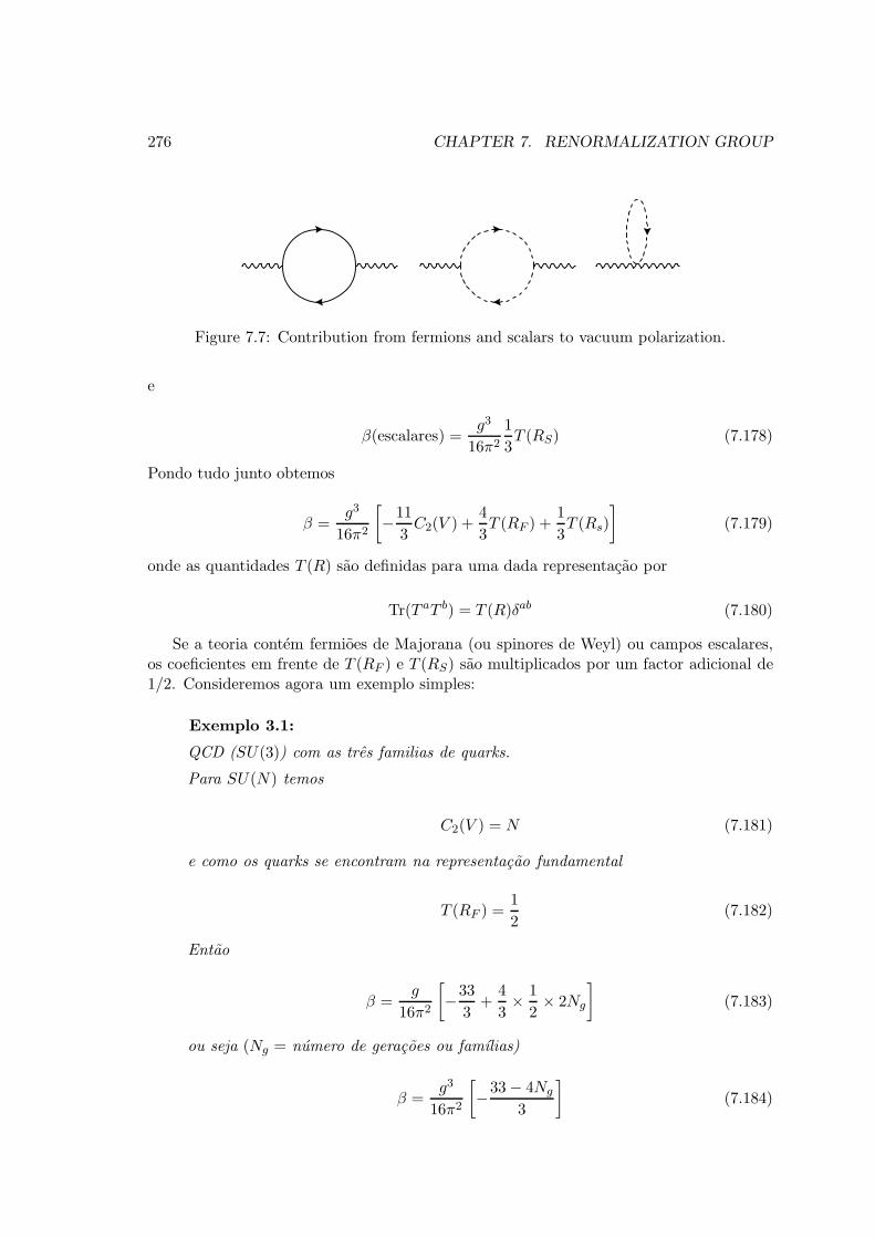
276 CHAPTER 7. RENORMALIZATION GROUP
Figure 7.7: Contribution from fermions and scalars to vacuum polarization.
e
β(escalares) =g3
16π21
3T (RS) (7.178)
Pondo tudo junto obtemos
β =g3
16π2
[−11
3C2(V ) +
4
3T (RF ) +
1
3T (Rs)
](7.179)
onde as quantidades T (R) sao definidas para uma dada representacao por
Tr(T aT b) = T (R)δab (7.180)
Se a teoria contem fermioes de Majorana (ou spinores de Weyl) ou campos escalares,os coeficientes em frente de T (RF ) e T (RS) sao multiplicados por um factor adicional de1/2. Consideremos agora um exemplo simples:
Exemplo 3.1:
QCD (SU(3)) com as tres familias de quarks.
Para SU(N) temos
C2(V ) = N (7.181)
e como os quarks se encontram na representacao fundamental
T (RF ) =1
2(7.182)
Entao
β =g
16π2
[−33
3+
4
3× 1
2× 2Ng
](7.183)
ou seja (Ng = numero de geracoes ou famılias)
β =g3
16π2
[−33− 4Ng
3
](7.184)

7.3. EFFECTIVE GAUGE COUPLINGS 277
Portanto SU(3) sera assimptoticamente livre se
33− 4Ng > 0 (7.185)
ou ainda
Ng <33
4→ Ng ≤ 8 (7.186)
Sao portanto permitidas 8 famılias ou seja 16 tripletos de SU(3).
7.3.3 The vacuum of a NAGT as a paramagnetic medium (µ > 1)
Um argumento recente (Nielsen 1981, Hughs 1981) permite compreender melhor o quese passa de diferente nas teorias de gauge nao abelianas para que elas tenham liberdadeassimptotica. Primeiro o facto de a carga diminuir a curta distancia pode ser interpretadocomo um anti - shielding do vacuo, isto e
ε < 1 (7.187)
O problema em compreender o que se passa resulta do facto de nao conhecermossubstancias3 com ε < 1. Contudo o vacuo deve ser invariante relativista e portanto deveter uma permeabilidade µ tal que (estamos a fazer c = 1)
µε = 1 (7.188)
Assim o antiscreening corresponde a µ > 1. Portanto o vacuo duma teoria de gauge naoabeliana e um paramagnetico e este conceito pode ser compreendido mais facilmente.
A permeabilidade magnetica pode ser calculada calculando a densidade de energia dovacuo num campo exterior
u0 =1
2µB2ext (7.189)
Nielsen e Hughes mostraram que µ = 1 + χ onde a susceptibilidade χ e dada por
χ ∼ (−1)2sq2∑
s3
(−1
3+ γ2s23
)(7.190)
onde s e o spin, q a carga, γ a razao giromagnetica e s3 a projeccao de spin na direccaodo campo magnetico externo. Assim para escalares, fermioes e campos de gauge obtemos
Escalares
χS ∼ −1
3q2S < 0 (diamagnetico) (7.191)
3Em QED a carga aumenta a curta distancia e portanto o vacuo e um dielectrico normal ε>1.

278 CHAPTER 7. RENORMALIZATION GROUP
Fermioes (γF = 2)
χF ∼ (−1)q2F 2
(−1
3+ 1
)= −4
3q2F (diamagnetico) (7.192)
Bosoes de gauge (γV = 2)
χV ∼ q2V 2
(−1
3+ 4
)=
22
3q2V (paramagnetico) (7.193)
e portanto
χTotal ∼22
3q2V − 4
3q2F − 1
3q2S (7.194)
Comparando com a funcao β podemos fazer a correspondencia
q2V → 1
2C2(V )
q2F → T (RF )
q2S → T (RS) (7.195)
o que permite compreender o vacuo das teorias de gauge nao abelianas como um meioparamagnetico.
7.4 Renormalization group applications
We consider the Grand Unified Theory (GUT) with the gauge group SU(5), that is
SU(5) ⊃ SUc(3)× SUL(2) × UY (1) . (7.196)
The unification takes place at the GUT scale MX . Using the renormalization groupequations and the low energy data on the coupling constants, it is possible to determinethe scale MX as well as other predictions for the theory at the low scale, which we taketo be the scale MZ . For this we need to know how the different coupling constants evolvewith the scale.
7.4.1 Scale MX
We start by writing the covariant derivatives for the unified theory and for the theory withthe broken symmetry.
SU(5) : Dµ = ∂µ + ig5
23∑
a=0
Aaµλa
2(7.197)

7.4. RENORMALIZATION GROUP APPLICATIONS 279
SU(3)× SU(2)× U(1) : Dµ = ∂µ + ig3
8∑
α
Gaµλ
2
a
+ig2
3∑
α
Aaµσ
2
a+ ig′
Y
2Bµ (7.198)
At the scale MX where the unification takes place we have
g5 = g3 = g2 = g1 (7.199)
where g1 is the coupling constant of the abelian subgroup of SU(5). However for theabelian groups there are no constraints in the normalization of the generators, and there-fore the the generator λ0 of that U(1) can be normalized in a different way from thehypercharge. We must have
g1λ0 = g′Y (7.200)
As λ0 is a generator of SU(5) it is normalized according to
TF (λaλb) = 2δab (7.201)
that is, for the fundamental representation we must have
λ0 =1√15
22
2−3
−3
(7.202)
Now, for the fundamental representation, we have
5 =
d1
d2
d3
e+
νce
R
(7.203)
and the hypercharge4 can be read directly. We obtain,
Y =
−2/3−2/3
−2/31
1
(7.204)
4Remember that our convention is such that Q = T3 +Y
2.

280 CHAPTER 7. RENORMALIZATION GROUP
Therefore Y = −√
53λ
0 and g′ = −√
35g1. This allows to determine sin2 θW at the GUT
scale MX ,
sin2 θW (MX) =g′2
g2 + g′2=
35g1
g2 +35g1
=3
8(7.205)
Also, for future reference, we note that
g′2 =3
5g21 . (7.206)
7.4.2 Scale MZ
Let us look now at what happens at the scaleMZ . The evolution of the coupling constantsis governed by the RGE equations for the three gauge groups in the broken phase
dgidt
= βi (7.207)
These β functions are given by
βi =g3i
16π2
−11
3C2(V ) +
∑
j
4
3T (RFj) +
∑
k
1
3T (RSk)
(7.208)
where the sums are over all the fermion and scalar physical states of the theory at a givenscale. Given the form of Eq. (7.208), it is usual to define
βi ≡1
16π2big
3i (7.209)
and therefore the bi are defined by the bracket in Eq. (7.208). Before we evaluate themlet us introduce Eq. (7.209) into Eq. (7.207). We get
dgidt
=bi
16π2g3i (7.210)
Let us solve this equations before we evaluate the beta function coefficients bi. For thatit is usual to introduce the generalization of the fine structure constant, that is, we define
αi ≡g2i4π
(7.211)
Multiplying both sides of Eq. (7.210) by gi and doing some trivial algebra we get,
dαidt
=bi2π
α2i (7.212)
Rearranging and integrating between some initial (µi), and final scale (µf ), we get
∫ f
i
dαiα2i
=bi2π
∫ f
idt (7.213)
7.4. RENORMALIZATION GROUP APPLICATIONS 281
or5 [− 1
αi
]f
i
=bi2π
(tf − ti) =bi2π
ln
(µfµi
)(7.214)
and finally
α−1i (µf ) = α−1i (µi)−bi4π
ln
(µ2fµ2i
)(7.215)
As at the unification scale MX we have, by definition (see Eq. (7.199)), that
α1 = α2 = α3 = α5 (7.216)
where α5 is the SU(5) unified value, and we can write the final solution
α−1i (µ) = α−15 +bi4π
ln
(M2X
µ2
), i = 1, 2, 3 (7.217)
We can rewrite these equations in terms of electromagnetic fine structure constant α(µ)and of the strong coupling equivalent αsµ), that are measured at the weak scale, to obtain
α−1s (µ) = α−15 +b34π
ln
(M2X
µ2
)
α−1(µ) sin2 θW (µ) = α−15 +b24π
ln
(M2X
µ2
)
35 cos2 θW (µ)α−1(µ) = α−15 +
b14π
ln
(M2X
µ2
)(7.218)
From these equations we obtain,
lnM2X
µ2=
12π
−8b3 + 3b2 + 5b1
[1
α(µ)− 8
3
1
αs(µ)
](7.219)
That allows to determine MX , once α(µ) and αs(µ) are known, at a given scale µ, and
sin2 θW (µ) =3(b2 − b3)
5b1 + 3b2 − 8b3+
5(b1 − b2)
5b1 + 3b2 − 8b3
α(µ)
αS(µ)(7.220)
which allows to determine sin2 θW at the scale µ = MZ , once α(MZ) and αs(MZ) areknown. Finally we can also solve for the value of α−15 . We get
α−15 = α−1(µ)1
5b1 + 3b2 − 8b3
[−3b3 + (5b1 + 3b2)
α(µ)
αS(µ)
](7.221)
Now we turn to the evaluation of the coefficients bi first in the Standard Model (SM)and the in the Minimal Supersymmetric Standard Model (MSSM).
5Remember that t = ln(µ).

282 CHAPTER 7. RENORMALIZATION GROUP
Standard Model
In the SM we have the gauge fields, Ng = 3 families of leptons, NF = 2Ng = 6 quarkflavours and one Higgs. With this information we can find the coefficients bi for the SMusing the definition
bi = −11
3C2(Vi) +
∑
j
2
3T (RFj ) +
∑
k
1
3T (RSk) (7.222)
where we have modified Eq. (7.208), as the sum in the fermions is done separately foreach quirality. This is important for the SM as the model is described in terms of left andright-handed fermions.
• SU(3)
For SU(3), we have C2(V3) = 3 and the quarks are in the fundamental representation,therefore T (RFj ) = 1/2. Then the counting goes as follows,
b3 = −11
3× 3
︸ ︷︷ ︸Gauge
+ Ng ×
2
3× 1
2× (2 + 1 + 1)
︸ ︷︷ ︸quarks
= −7 (7.223)
where the meaning of (2 + 1 + 1) is that we count the up and down components of each(SU(2)L) doublet and then the corresponding right-handed quarks for each generation.
• SU(2)
For the SU(2) we get
b2 = −11
3× 2
︸ ︷︷ ︸Gauge
+ Ng ×
Nc ×
2
3× 1
2︸ ︷︷ ︸quarksL
+2
3× 1
2︸ ︷︷ ︸leptons
+
1
3× 1
2︸ ︷︷ ︸Higgs
= −19
6(7.224)
where Nc = 3 is the number of colours.
• U(1)
Finally for the U(1) part, with the correct normalization, we have
b1 =3
5×
23×∑
fL,fR
(Y
2
)2
+1
3×∑
scalars
(Y
2
)2 (7.225)

7.4. RENORMALIZATION GROUP APPLICATIONS 283
and therefore,
b1 =3
5×
Ng ×
2
3×(−1
2
)2
× 2
︸ ︷︷ ︸LeptonsL
+2
3× (−1)2
︸ ︷︷ ︸LeptonsR
+Nc ×2
3×(1
6
)2
× 2
︸ ︷︷ ︸QuarksL
+Nc ×2
3×(2
3
)2
︸ ︷︷ ︸Up−QuarksR
+Nc ×2
3×(1
3
)2
︸ ︷︷ ︸Down−QuarksR
+
1
3×(1
2
)2
× 2
︸ ︷︷ ︸Higgs
= 4 +1
10︸︷︷︸Higgs
=41
10(7.226)
So in summary we have for the SM,
b1 =41
10, b2 = −19
6, b3 = −7 (7.227)
Now let us look to see what are the results for MX , sin2 θW (MZ) and α−15 . We will
use the current values from the Particle Data Group. These are (without worrying abouterrors)6
α−1(MZ) = 127.916, αs(MZ) = 0.118, MZ = 91.1896 GeV (7.228)
we get
MX = 6.7 × 10¹⁴ GeV, sin2 θW (MZ) = 0.208, α−15 = 41.48 (7.229)
At the time that this GUT model was proposed by the first time, the constants werenot known so precisely as today. Also the bound on the lifetime of the proton was muchlower than today. So at that time the model was completely consistent. However aftermany years of dedicated experiments for find the decay of the proton, the lower limit wassubstantially improved and also after LEP the coupling constants are known with greaterprecision. So today the value for MX is too low, the same being true for the value ofsin2 θW (MZ) (the best value today is around sin2 θW (MZ) = 0.230 7).
This can be seen very clearly if we use Eq. (7.215), with µi =MZ and plot the α−1i asa function of ln(µ2/M2
Z). This is shown in Fig. 7.8. We clearly see that the agreement isquite poor with today’s values.
Minimal Supersymmetric Standard Model
Let us now turn to the MSSM. Below the GUT scale the gauge group is the same as inthe SM, but the particle content is larger, more than duplicated in relation to the SM.We summarize in the Table 7.1 the particle content and their quantum numbers underG = SUc(3) ⊗ SUL(2)⊗ UY (1).
6Not only errors but also the difference between different renormalization schemes. Also this discussionis at one-loop level.
7Again, without discussing the very small errors and the dependence on the renormalization scheme.

284 CHAPTER 7. RENORMALIZATION GROUP
-1
(GeV)
1-1
2-1
3-1
0
10
20
30
40
50
60
100 104 108 1012 1016
a
a
aai
µ
Figure 7.8: Evolution of αi as function of the scale µ in the Standard Model for a SU(5)minimal GUT theory.
With the values in Table 7.1 we can calculate the contribution of the various particlesto the bi coefficients. We will do it in succession for the three groups and for the differentsupermultiplets.
• SU(3)
– Gauge Supermultiplet
We first do it in general for any gauge group and then apply it to the cases of interest.The gauge multiplet has a gauge boson contributing with
b gauge boson = −11
3C2(V ) (7.230)
and the left-handed gauginos in the adjoint representation of the gauge group. Thesetherefore contribute
b gauginos =2
3C2(V ) (7.231)
and thereforeb gauge SM = −3 C2(V ) (7.232)
where SM stands here for super-multiplet. Applying now to SU(3) we get
b gauge SM3 = −9 (7.233)
– Left-handed Lepton Supermultiplet
bLeptonsL SM3 = 0 (7.234)

7.4. RENORMALIZATION GROUP APPLICATIONS 285
Supermultiplet SUc(3) ⊗ SUL(2)⊗ UY (1)Quantum Numbers
V1 ≡ (λ′,W µ1 ) (1, 1, 1)
V2 ≡ (λa,W µa2 ) (1, 3, 0)
V3 ≡ (gb,W µb3 ) (8, 1, 0)
Li ≡ (L, L)i (1, 2,−1)
Ri ≡ (ℓR, ℓcL)i (1, 1, 2)
Qi ≡ (Q,Q)i (3, 2, 13)
Di ≡ (dR, dcL)i (3, 1, 23)
Ui ≡ (uR, ucL)i (3, 1,−4
3 )
Hd ≡ (Hd, Hd) (1, 2,−1)
Hu ≡ (Hu, Hu) (1, 2, 1)
Table 7.1: Particle content of the MSSM. Note that Q = T3 + Y/2.
– Right-handed Lepton Supermultiplet
bLeptonsR SM3 = 0 (7.235)
– Left-handed Quark Supermultiplet
bQuarksL SM3 =
2
3× 1
2× 2
︸ ︷︷ ︸QuarksL
+1
3× 1
2× 2
︸ ︷︷ ︸SquarksL
= 1 (7.236)
– Right-handed Up-Quark Supermultiplet
bUp−QuarkR SM3 =
2
3× 1
2︸ ︷︷ ︸Up−QuarksR
+1
3× 1
2︸ ︷︷ ︸Up−SquarksR
=1
2(7.237)
– Right-handed Down-Quark Supermultiplet
bDown−QuarkR SM3 =
2
3× 1
2︸ ︷︷ ︸Down−QuarksR
+1
3× 1
2︸ ︷︷ ︸Down−SquarksR
=1
2(7.238)
– Up type Higgs Supermultiplet

286 CHAPTER 7. RENORMALIZATION GROUP
bUp−Higgs SM3 = 0 (7.239)
– Down type Higgs Supermultiplet
bDown−Higgs SM3 = 0 (7.240)
• SU(2)
Gauge Supermultiplet
We get
b gauge SM2 = −6 (7.241)
– Left-handed Lepton Supermultiplet
bLeptonsL SM2 =
2
3× 1
2︸ ︷︷ ︸LeptonsL
+1
3× 1
2︸ ︷︷ ︸SleptonsL
=1
2(7.242)
– Right-handed Lepton Supermultiplet
bLeptonsR SM2 = 0 (7.243)
– Left-handed Quark Supermultiplet
bQuarksL SM2 = Nc
2
3× 1
2︸ ︷︷ ︸QuarksL
+Nc1
3× 1
2︸ ︷︷ ︸SquarksL
= Nc1
2=
3
2(7.244)
– Right-handed Up-Quark Supermultiplet
bUp−QuarkR SM2 = 0 (7.245)
– Right-handed Down-Quark Supermultiplet
bDown−QuarkR SM2 = 0 (7.246)
– Up type Higgs Supermultiplet

7.4. RENORMALIZATION GROUP APPLICATIONS 287
bUp−Higgs SM2 =
1
3× 1
2︸ ︷︷ ︸Higgsu
+2
3× 1
2︸ ︷︷ ︸Higgsinou
=1
2(7.247)
– Down type Higgs Supermultiplet
bDown−Higgs SM2 =
1
3× 1
2︸ ︷︷ ︸Higgsd
+2
3× 1
2︸ ︷︷ ︸Higgsinod
=1
2(7.248)
• U(1)
Gauge Supermultiplet
We get
b gauge SM1 = 0 (7.249)
– Left-handed Lepton Supermultiplet
bLeptonsL SM1 =
3
5×
2
3×(−1
2
)2
× 2
︸ ︷︷ ︸LeptonsL
+1
3×(−1
2
)2
× 2
︸ ︷︷ ︸SleptonsL
=
3
10(7.250)
– Right-handed Lepton Supermultiplet
bLeptonsR SM1 =
3
5×
2
3× (−1)2
︸ ︷︷ ︸LeptonsR
+1
3× (−1)2
︸ ︷︷ ︸SleptonsR
=
3
5(7.251)
– Left-handed Quark Supermultiplet
bQuarksL SM1 =
3
5×Nc×
2
3×(1
6
)2
× 2
︸ ︷︷ ︸QuarksL
+1
3×(1
6
)2
× 2
︸ ︷︷ ︸SquarksL
= Nc×
3
5× 1
18=
1
10(7.252)
– Right-handed Up-Quark Supermultiplet

288 CHAPTER 7. RENORMALIZATION GROUP
bUp−QuarksR SM1 =
3
5×Nc ×
2
3×(2
3
)2
︸ ︷︷ ︸Up−QuarksR
+1
3×(2
3
)2
︸ ︷︷ ︸Up−SquarksR
= Nc ×
3
5× 4
9=
4
5(7.253)
– Right-handed Down-Quark Supermultiplet
bDown−QuarksR SM1 =
3
5×Nc×
2
3×(−1
3
)2
︸ ︷︷ ︸Down−QuarksR
+1
3×(−1
3
)2
︸ ︷︷ ︸Down−SquarksR
= Nc×
3
5× 1
9=
1
5(7.254)
– Up type Higgs Supermultiplet
bHiggsu SM1 =
3
5×
1
3×(1
2
)2
× 2
︸ ︷︷ ︸Higgsu
+2
3×(1
2
)2
× 2
︸ ︷︷ ︸Higgsu
=
3
5× 1
2=
3
10(7.255)
– Down type Higgs Supermultiplet
bHiggsd SM1 =
3
5×
1
3×(−1
2
)2
× 2
︸ ︷︷ ︸Higgsd
+2
3×(−1
2
)2
× 2
︸ ︷︷ ︸Higgsd
=
3
5× 1
2=
3
10(7.256)
Now we put everything together to obtain fro the MSSM,
b1 =Ng ×(
3
10+
3
5+
1
10+
4
5+
1
5
)+
3
10+
3
10= 3× 2 +
3
5=
33
5
b2 =− 6 +Ng ×(1
2+
3
2
)+
1
2+
1
2= 1
b3 =− 9 +Ng ×(1 +
1
2+
1
2
)= −3 (7.257)

7.4. RENORMALIZATION GROUP APPLICATIONS 289
Now let us look to see what are the results for MX , sin2 θW (MZ) and α−15 in theMSSM. Using the same inputs as for the SM, Eq. (7.228) 8 , we get
MX = 2.1 × 10¹⁶ GeV, sin2 θW (MZ) = 0.231, α−15 = 24.27 (7.258)
we immediately see that these values are quite good. This can be seen very clearly if weuse Eq. (7.215), with µi =MZ and plot the α−1i as a function of ln(µ2/M2
Z). This is shownin Fig. 7.9 and the agreement is excellent.
-1
(GeV)
1-1
2-1
3-1
0
10
20
30
40
50
60
100 104 108 1012 1016
a
a
a
ai
µ
Figure 7.9: Evolution of αi as function of the scale µ in the MSSM for a SU(5) minimalGUT theory.
We can still go a step further. We know that supersymmetry must be broken abovethe electroweak scale, so what we have done in Fig. 7.9 is not quite correct because weare running with the MSSM content down to the weak scale. Of course each particle willdecouple at its mass, but assuming that their masses are not much different we can assumethat there will a scale MSUSY, below which we will have the SM RGEs. We can redo thecalculation taking now the evolved SM values at MSUSY as the boundary conditions forthe MSSM evolution. In Fig. and Fig. the results are shown for various values of theSUSY scale. We see from these results that if the SUSY scale is much higher than, say1 TeV, the good agreement starts do disappear. Before we end we should emphasize thatthese are one loop results, without many fine details, like thresholds (talking in accountthat not all the supersymmetric particles decouple at the same scale) and the importanttwo-loop effects.
8Again we do not take into account errors and the difference between different renormalization schemes.Also this discussion is at one-loop level and the effects of the supersymmetric particles not decoupling atthe same scale (thresholds) are not taken in account.

290 CHAPTER 7. RENORMALIZATION GROUP
-1
(GeV)
1-1
2-1
3-1
0
10
20
30
40
50
60
100 104 108 1012 1016
a
a
a
a i
µ-1
(GeV)
1-1
2-1
3-1
0
10
20
30
40
50
60
100 104 108 1012 1016
a
a
a
a iµ
Figure 7.10: Evolution of αi as function of the scale in the MSSM for a SU(5) minimalGUT theory. On the left panel MSUSY = 500 GeV and on the right panel MSUSY = 1000GeV.
-1
(GeV)
1-1
2-1
3-1
0
10
20
30
40
50
60
100 104 108 1012 1016
a
a
a
a i
µ
-1
(GeV)
1-1
2-1
3-1
0
10
20
30
40
50
60
100 104 108 1012 1016
a
a
a
a i
µ
Figure 7.11: Evolution of αi as function of the scale in the MSSM for a SU(5) minimalGUT theory. On the left panel MSUSY = 104 GeV and on the right panel MSUSY = 108
GeV.

Problems 291
Problems for Chapter 7
3.1 Verifique a equacao 7.161. Para isso note que βi = dgi
dt onde βi e calculada a partirdos diagramas seguintes
ii
i
i
i
3.2 Calcule em subtracao mınima (MS) a constante de renormalizacao Z3 para QED,equacao 7.166.
3.3 Calcule em MS a constante de renormalizacao Z3 em electrodinamica escalar, equacao7.168.
3.4 Considere uma teoria nao abeliana com grupo de simetria G e sem materia. Calculeas constantes de renormalizacao do propagador ZA, e do vertice triplo Z1.
3.5 Considere uma teoria nao abeliana em interaccao com campos escalares e fermioni-cos. Calcule a contribuicao destes campos para ZA e Z1. Utilize estes resultadosjuntamente com os resultados do problema 3.4 para determinar a funcao β do grupode renormalizacao para essa teoria.
3.6 Considere o modelo padrao das interaccoes electrofracas e fortes. Considerando todosos campos do modelo (incluindo os Higgs) calcule os coeficientes b1, b2 e b3 definidosna equacao (tc2-3.201).
3.7 Considere agora o modelo padrao supersimetrico mınimo (MSSM). Calcule os coefi-cientes b1, b2 e b3 definidos na equacao (tc2-3.201). Refaca a analise da convergencia

292 CHAPTER 7. RENORMALIZATION GROUP
das constantes de acoplamento no quadro duma teoria de grande unificacao super-simetrica com o grupo SU(5).

Appendix A
Path Integral in QuantumMechanics
A.1 Introduction
A formulacao usual e dada pela equacao de Schrodinger
ih∂
∂t|a(t)〉 = H |a(t)〉 (A.1)
onde
H =P 2
2m+ V (Q) (A.2)
e
[Q,P ] = ih (A.3)
Esta formulacao e equivalente a uma outra definida em termos de integrais de caminho.Para isso baseamo-nos na observacao que em mecanica quantica sabemos responder aqualquer pergunta sobre o sistema se soubermos calcular as amplitudes de transicao
⟨b(t′)|a(t)
⟩= 〈b| e−iH(t′−t) |a〉 (A.4)
Sao estas amplitudes de transicao que sao definidas em termos de integrais de caminho.Conforme a representacao escolhida para os estados |a〉 e |b〉 as expressoes para o integral decaminho vem diferentes. Assim vamos analisar separadamente os casos das representacoesno espaco das configuracoes (coordenadas), no espaco de fase e por meio de estados coe-rentes (espaco de Bargmann-Fock).
A.2 Configuration space
Introduzimos os estados |q〉 e |p〉 tais que
293

294 APPENDIX A. PATH INTEGRAL IN QUANTUM MECHANICS
Q |q〉 = q |q〉 ; P |p〉 = p |p〉
〈q′|q〉 = δ(q′ − q) ; 〈p′|p〉 = δ(p′ − p)
〈q|p〉 = 〈p|q〉∗ = 1√2πeipq (A.5)
Entao
〈qf , tf |qi, ti〉 =∫
D(q)eih
∫ tfti
dtL(q,q) (A.6)
onde D e uma medida de integracao definida pelo limite
D(q) = limn→∞
n−1∏
1
dqp
[nme−iπ/2
2π(tf − ti)
]n2
(A.7)
sendo n o numero de intervalos em que se fez a particao do intervalo (ti, tf ). O limiten→ ∞ e bastante complicado e so existe prova matematica para certas classes de potenci-ais. A Eq. (A.6) permite uma interpretacao da mecanica classica como limite da mecanicaquantica. De facto quando h → 0 a maior contribuicao para a amplitude vem das tra-jectorias que minimizam a ac cao, isto e, as trajectorias classicas. A mecanica quantica eentao vista como o estudo das flutuacoes a volta da trajectoria classica.
A.2.1 Matrix elements of operators
Usando a propriedade dos integrais de caminho
∫D(q)eiS(f,i) =
∫dq(t)
∫D(q)eiS(f,t)
∫D(q)eiS(t,i) (A.8)
onde ti < t < tf , e facil mostrar que
〈qf , tf | O(t) |qi, ti〉 =
∫dq′dq′′
∫D(q)eiS(qf ,tf ;q
′′,t)
⟨q′′∣∣O∣∣q′⟩ ∫
D(q)eiS(q′,t;qi,ti) (A.9)
Entao se O for diagonal no espaco das coordenadas, isto e, se
⟨q′′∣∣O∣∣q′⟩= O(q′)δ(q′ − q′′) (A.10)
obtemos
〈qf , tf | O |qi, ti〉 =∫
D(q) eiS(f,i)O(q(t)) (A.11)

A.2. CONFIGURATION SPACE 295
A.2.2 Time ordered product of operators
Seja O1(t1)O2(t2) · · · On(tn) com t1 ≥ t2 ≥ · · · ≥ tn. Entao e facil de mostrar que aordenacao no tempo e automatica no integral de caminho, isto e,
〈qf , tf | O1(t1)O2(t2) · · · On(tn) |qi, ti〉 =∫
D(q)eiS(f,i)O1O2 · · · On (A.12)
Este resultado e particularmente importante, pois permitira escrever as funcoes de Greende produtos de operadores ordenados no tempo como simples integrais de caminho deprodutos dos equivalentes classicos desses operadores.
A.2.3 Exact results I: harmonic oscillator
Para alguns potenciais e possıvel calcular exactamente o limite introduzido em (A.5). Paraesses casos o integral de caminho e portanto perfeitamente bem definido. Esses potenciaisnao sao muitos, mas sao particularmente importantes. Para o seguimento interessa-nosdiscutir dois deles. O primeiro e o oscilador harmonico definido pelo potencial
V (Q) = mω2
2Q2 (A.13)
Para este caso obtem-se, (os integrais sao gaussianos e por isso podem ser explicitamentecalculados)
〈f |i〉 =(mωe−iπ/2
2π sinωt
) 12
exp
imω
2
[(q2f + q2i ) cotωt−
2qfqisinωt
](A.14)
Este resultado vai ser util adiante.
A.2.4 Exact results II: external force
Consideremos agora uma forca exterior tal que o potencial e dado por
V (Q) = −QF (t) (A.15)
Neste caso obtemos
〈f |i〉F =
[me−iπ/2
2π(tf − ti)
] 12
eiS(f,i) (A.16)
onde S(f, i) e a accao calculada ao longo da trajectoria classica,
S(f, i) =m
2
(qf − qi)2
tf − ti+
∫ tf
ti
dtF (t)
(qf
t− titf − ti
+ qitf − t
tf − ti
)

296 APPENDIX A. PATH INTEGRAL IN QUANTUM MECHANICS
+1
2m
∫ tf
ti
∫ tf
ti
dt′dt′′F (t′)G(t′, t′′)F (t′′) (A.17)
onde G(t′, t′′) = t′t′′
T −Inf(t′, t′′) e a funcao de Green simetrica para o problema q..= F (t)/m
com as condicoes na fronteira G(0, t′′) = G(t′, 0) = 0.
A.2.5 Perturbation theory
A importancia do resultado exacto para a forca exterior deve-se ao facto que usandoesse resultado podemos formalmente resolver o problema dum potencial qualquer. Paraisso notemos que a derivacao funcional em realacao a fonte F (t) faz baixar Q(t). Maisexplicitamente
〈f |Q(t) |i〉F =δ
iδF (t)〈f |i〉F (A.18)
onde 〈|〉F significa calculado na presenca da fonte exterior (i.e. para o hamiltonianoH = P 2/2m−QF (t)). Entao para um potencial arbitrario V (q) temos
〈f |i〉 =
∫D(q)e
i∫ tfti
dt[ 12mq2−V (q)]
= exp
−i∫ tf
ti
dtV
[δ
iδF (t)
]〈f |i〉F
∣∣∣F=0
(A.19)
Esta expressao formal torna-se muito util quando a exponencial e expandida em serie.Entao todos os integrais sao do tipo gaussiano e podem ser exactamente executados.Obtemos assim a teoria das perturbacoes. Claro que so tera significado se houver umparametro pequeno no potencial. E importante notar que enquanto se faca teoria das per-turbacoes nao ha qualquer problema com a indefinicao matematica do integral de caminho,pois todas as integracoes sao gaussianas.
A.3 Phase space formulation
Para este caso obtemos
〈qf , tf |qi, ti〉 =∫
D(p, q)ei∫ tfti
dt[pq−h(p,q)
](A.20)
onde h(p, q) e o hamiltoniano classico e a medida e dada pelo limite
D(p, q) = limn→∞
n∏
1
dps
n−1∏
1
dqr
(2π)n(A.21)

A.4. BARGMANN-FOCK SPACE (COHERENT STATES) 297
A fase da exponencial e novamente a accao classica expressa nas variaveis canonicas pe q. Se h(p, q) depender quadraticamente de p como e usual, pode-se fazer a integracaogaussiana em p e a expressao reduz-se a do caso anterior, equacao (A.4).
A.4 Bargmann-Fock space (coherent states)
Nesta representacao usamos funcoes analıticas de variavel complexa para descrevermos osoperadores a e a† ( [a, a†] = 1). A correspondencia e feita do modo seguinte. As funcoesanalıticas geram um despaco de Hilbert com o produto interno definido por
〈g|f〉 ≡∫dzdz
2πie−zz g(z)f(z) (A.22)
Os operadores a e a† sao representados neste espaco por
a→ ∂
∂z
a† → z (A.23)
Dado um estado |f〉, representado pela funcao f(z), a accao do operador A em |f〉 produzoutro estado que tambem pode ser representado por funcoes analıticas. Se designarmospor g(z) essa funcao temos
g(z) ≡ 〈z|A |f〉 ≡∫dξdξ
2πie−ξξA(z, ξ)f(ξ) (A.24)
onde A(z, ξ) e o kernel do operador A. Uma representacao explicita para o kernel e facilde obter. Para isso introduzimos os estados |n〉, definidos por
|n〉 = a†n√n!
|0〉 (A.25)
E facil de verificar (ver Problema A.2) que com a definicao de produto interno acimaintroduzida estes estados sao ortonormados, isto e 〈fm|fn〉 = δmn.
Entao
〈z|A |f〉 =∑
n,m
zn√n!
〈n|A |m〉 〈m|f〉
=∑
n,m
zn√n!
An,m
∫dξdξ
2πie−ξξ
ξm√m!f(ξ)
=
∫dξdξ
2πie−ξξ
[∑
n,m
zn√n!An,m
ξm√m!
]f(ξ) (A.26)

298 APPENDIX A. PATH INTEGRAL IN QUANTUM MECHANICS
Portanto
A(z, ξ) ≡∑
n,m
zn√n!An,m
ξm√m!
(A.27)
O kernel de qualquer operador e assim obtido desde que se conhecam os seus elementosde matriz na base |n〉.
Ja vimos como se representam estados e operadores. Vamos ver como representarprodutos de operadores. Sejam dois operadores A1 e A2 e um estado |f〉. Seja ainda
g(η) = 〈η|A2 |f〉 =∫dξdξ
2πie−ξξA2(η, ξ)f(ξ) (A.28)
Entao
〈z|A1 |g〉 =
∫dξdξ
2πie−ξξA1(z, η)g(η)
=
∫dηdη
2πi
dξdξ
2πie−ξξe−ηη A1(z, η)A2(η, ξ)f(ξ)
=
∫dξdξ
2πie−ξξ
[∫dηdη
2πie−ηη A1(z, η)A2(η, ξ)
]f(ξ)
=
∫dξdξ
2πie−ξξ A3(z, ξ)f(ξ) (A.29)
Portanto o kernel do operador A3 = A1A2 e obtido por convolucao dos kerneis de A1 eA2, isto e
A3(z, η) =
∫dηdη
2πie−ηη A1(z, η)A2(η, ξ) (A.30)
A.4.1 Normal form for an operator
Como ja sabemos representar estados, operadores e produtos de operadores ja temos toosos ingredientes para fazer mecanica quantica neste espaco. Ha contudo um outro assuntoque e importante tendo em atencao que pretendemos aplicar este formalismo em teoriaquantica dos campos. Trata-se da forma normal dum operador1. O operador A na suaforma normal e definido por
A =∑
n,m
ANn,ma†nam√n!√m!
(A.31)
isto e, os operadores de destruicao estao a direita dos operadores de criacao. O kernelnormal e definido por
1Notar que em teoria quantica dos campos tem que se proceder ao ordenamento normal do hamiltonianopara definir o zero da energia.

A.4. BARGMANN-FOCK SPACE (COHERENT STATES) 299
AN (z, z) ≡∑
n,m
zn√n!
ANn,mzm√m!
(A.32)
isto e, e obtido por subtituicao directa dos operadores de destruicao por z e dos de criacaopor z. Para um operador dado na sua forma normal este e o kernel imediato de obter. Econtudo diferente do kernel atras definido. Para ver a relacao entre eles notemos a seguinterelacao
f(z) =∑
n
z√n!
〈n|f〉
=∑
n
∫dξdξ
2πie−ξξ
znξn
n!f(ξ)
=
∫dξdξ
2πie−ξξ ezξ f(ξ) (A.33)
O kernel ezξ e portanto uma funcao delta neste espaco. Usando este resultado obtemos
〈z|A |f〉 =∑
n,m
ANn,m√n!√m!
zndm
dzmf(z)
=∑
n,m
ANn,m√n!√m!
∫dξdξ
2πie−ξξ ezξ znξmf(ξ)
=
∫dξdξ
2πie−ξξ ezξ AN (z, ξ)f(ξ) (A.34)
donde resulta
A(z, ξ) = ezξ AN (z, ξ) (A.35)
Esta relacao e muito importante pois permite imediatamente escrever o kernel dum ope-rador qualquer uma vez que seja conhecida a sua forma normal. Isto e particularmenteutil em teoria quantica dos campos onde o hamiltoniano e dado na sua forma normal.
A.4.2 Evolution operator
Podemos obter agora a expressao para o operador de evolucao nesta representacao. Deacordo com aquilo que acabamos de dizer, para um intervalo infinitesimal, devemos terpara o kernel de U
U(z, ξ,∆t) = ezξ e−i∆t h(z,ξ) (A.36)

300 APPENDIX A. PATH INTEGRAL IN QUANTUM MECHANICS
onde h(z, ξ) e o kernel normal obtido por substituicao directa dos operadores a† e a pelasvariaveis complexas z e ξ. Notar que quando ∆t→ 0 o kernel do operador de evolucao sereduz ao kernel da identidade, ezξ, que como vimos e a funcao δ neste espaco.
Para um intervalode tempo finito t = tf − ti, dividimos o intervalo em n intervalos
∆t =t
nz0 z1 z2 · · · zn−1 zn (A.37)
Entao
U(z1, z0) ≃ ez1z0−i∆th(z1,z0)
U(z2, z1) ≃ ez2z1−i∆th(z2,z1)...
......
U(zn, zn−1) ≃ eznzn−1−i∆th(zn,zn−1) (A.38)
Aplicando agora a regra de multiplicacao dos kerneis obtemos
U(zf , tf ; zi, ti) = limn→∞
∫ n−1∏
k=1
dzkdzk2πi
exp[ n∑
k=1
zk zk−1
−n−1∑
k=1
zkzk − i
n∑
k=1
h(zk, zk−1)∆t]
(A.39)
ou seja
U(zf , tf ; zi, ti) ≡∫
D(z, z) e12
(zfzf+zizi)+i∫ tfti[ 12i(zz−zz)−h(z,z)]dt (A.40)
Nesta expressao zf (tf ) e zi(ti) sao fixados pelas condicoes fronteiras mas zf (ti) e zi(tf )sao arbitrarios. A fase da exponencial e novamente a accao, agora escrita nas variaveiscomplexas z e z. Para ver isso basta lembrar que
1
2(pdq + qdp) =
1
2i(zdz − zdz) (A.41)
A.4.3 Exact results I: harmonic oscillator
Tambem aqui vamos analisar os casos importantes em que ha resultados exactos, nomeada-mente o oscilador hamonico e o caso das fontes externas. Comecemos pelo osciladorharmonico. O hamiltoniano e dado por
H0 = ω a†a (A.42)

A.4. BARGMANN-FOCK SPACE (COHERENT STATES) 301
Trata-se portanto dum caso em que o hamiltoniano e dado na forma normal. Este problemapode ser resolvido exactamente. Temos
U(zf , zi, t) = limn→∞
∫ n−1∏
k=1
dzkdzk2πi
exp[ n∑
k=1
zk zk−1
−n−1∑
k=1
zkzk − iωt
n
n∑
k=1
zkzk−1]
= limn→∞
∫ n−1∏
k=1
dzkdzk2πi
e[−XAX+XB+BX] (A.43)
onde
X =
z1z2...
zn−1
; X = (z1, z2, · · · , zn−1) (A.44)
e
B =
z0a0...0
; B = (0, 0, · · · , 0, zna) (A.45)
com z0 = zi e zn = zf . A matriz A de dimensao (n− 1)× (n− 1) e dada por
1 0 · · · · · · · · · · · ·−a 1 0 · · · · · · · · ·0 −a 1 0 · · · · · ·...
. . .. . .
. . .. . .
...· · · · · · 0 −a 1 0· · · · · · · · · 0 −a 1
(A.46)
onde se definiu
a ≡ 1− ihωt
n(A.47)
As (n − 1) integracoes gaussianas podem ser facilmente feitas usando o resultado (verProblema A.3),
∫ ∏ dzkdzk2πi
e−zAz+uz+zu = (detA)−1 euA−1u (A.48)
obtemos entao

302 APPENDIX A. PATH INTEGRAL IN QUANTUM MECHANICS
U0(zf , zi; t) = limn→∞
[(detA)−1 eBA
−1B]
= limn→∞
[(detA)−1 ezf zia
2(A−1)n−1,1
](A.49)
E facil de verificar que para a matriz A se tem
(A−1)k,m =
ak−m se k ≥ m
0 se k < m
(A.50)
e portanto
detA = 1 (A.51)
e
A−1n−1,1 = (−1)n(−a)n−2 (A.52)
donde se conclui que
limn→∞
a2(A−1)n−1,1 = limn→∞
(1− iωt
n
)n= e−iωt (A.53)
Obtemos entao finalmente
U0(zf , zi; t) = expzfzie
−iωt (A.54)
Podemos verificar que este resultado e da forma eiS onde S e a accao calculada ao longoda trajectoria classica. De facto a estacionaridade do expoente da exponencial da
δ
1
2(zfz(tf ) + z(ti)zi) +
∫ tf
ti
[zz − zz
2− iωzz
]dt
=1
2zf δz(tf ) +
1
2ziδz(ti)−
1
2zf δz(tf )−
1
2ziδz(ti)
+
∫ tf
ti
[δz(z − iωz)− δz(z + iωz)
]dt (A.55)
pois δzf = δzi = 0. As equacoes de movimento sao portanto
z − iωz = 0
z + iωz = 0
com
z(tf ) = zf
z(ti) = zi
(A.56)

A.4. BARGMANN-FOCK SPACE (COHERENT STATES) 303
que tem como solucao
z(t) = zi eiω(ti−t)
z(t) = zf eiωt−tf )
(A.57)
Substituindo estas solucoes no expoente obtemos
1
2[zfz(tf ) + ziz(ti)] +
∫ tf
ti
[1
2(zz − zz)− iωzz
]dt
= zfzi eiω(ti−tf )
= zfzi e−iωt (A.58)
para t ≡ tf − ti, como querıamos mostrar.
Um outro resultado importante do oscilador harmonico e que a evolucao dum estadosob a accao de H0 = ωa†a e particularmente simples neste espaco das funcoes de variavelcomplexa. Seja f(z) a representacao do estado |f〉. A evolucao debaixo de H0 e dada por
U0(t)f(z) =
∫dξdξ
2πie−ξξ ezξe
−iωt
f(ξ)
= f(ze−iωt) (A.59)
isto e, e reduzida a multiplicacao por e−iωt
z → z e−iωt (A.60)
Isto e importante para descrever a matriz S, em que os estados assimptoticos evoluem deacordo com o hamiltoniano livre.
A.4.4 Exact results II: external force
Seja o hamiltoniano
H = ωa†a− f(t)a† − f(t)a (A.61)
Este hamiltoniano tambem conduz a um resultado exacto. Usando os mesmos metodosque foram utilizados para o oscilador harmonico pode-se mostrar que neste caso tambemtemos
U(zf , zi; t) = eiS(f,i) (A.62)
onde S(f, i) e a accao calculada ao longo das trajectorias classicas (ver Problema A.1).

304 APPENDIX A. PATH INTEGRAL IN QUANTUM MECHANICS
A.5 Fermion systems
Vamos generalizar os resultados anteriores ao caso de sistemas de fermioes. Comecamoscom sistemas com dois nıveis com os operadores a† e a tais que
a†, a
= 1 ; a2 = a2† = 0 (A.63)
Para efectuar a construcao anterior vamos tentar representar estes operadores num espacode Hilbert de funcoes analıticas. Isto e possıvel se considerarmos funcoes (de facto polino-mios) com coeficientes complexos em duas variaveis que anticomutam η e η, designadaspor variaveis de Grassmann e que obedecem a
ηη + ηη = 0 ; η2 = η2 = 0 (A.64)
Entao qualquer funcao P (η, η) tera a forma
P (η, η) = p0 + p1η +∼p1η + p12ηη (A.65)
A.5.1 Derivatives
Neste espaco a derivacao e definida por (as derivadas sao esquerdas)
∂P
∂η=∼p1 + p12η
∂P
∂η= p1 − p12η (A.66)
De entre todas as funcoes nas variaveis η e η definimos o subconjunto das funcoes analıticastais que
∂
∂ηf = 0 (A.67)
isto e as funcoes analıticas tem a forma
f = f0 + f1η (A.68)
A.5.2 Dot product
No espaco das funcoes analıticas define-se o produto interno
(g, f) = g0 f0 + g1 f1 (A.69)
este produto interno pode ser representado por um integral desde que definamos a inte-gracao convenientemente (ver equacao (A.74)) .

A.5. FERMION SYSTEMS 305
A.5.3 Integration
A integracao nas variaveis de Grassmann e definida pelas relacoes
∫dη η =
∫dη η = 1
∫dη 1 =
∫dη 1 = 0 (A.70)
Notar que a integracao assim definida e semelhante a derivacao. De facto2
∫dη P = ∂P ;
∫dη P = ∂P
∫dηdη P = ∂∂P (A.72)
Devido a forma da equacao A.62 e claro que se tem
∂2= ∂2 = 0 (A.73)
e que portanto o integral duma derivada e zero. Consideremos agora a mudanca devariaveis nos integrais. Seja
(ηη
)= A
(ξ
ξ
)(A.74)
Entao obtemos
ηη = (A11ξ +A12ξ)(A21ξ +A22ξ)
= (A11A22 −A12A21)ξξ
= detA ξξ (A.75)
Pelo que
∫dηdηP (η, η) =
∫dξdξ(detA)−1Q(ξ, ξ) (A.76)
onde Q(ξ, ξ) e o polinomio que se obtem de P (η, η) por substituicao de η e η por ξ e ξ.
2Estamos a usar a notacao compacta
∂≡ ∂∂η
; ∂≡ ∂∂η
(A.71)
306 APPENDIX A. PATH INTEGRAL IN QUANTUM MECHANICS
Finalmente notemos que se definirmos a conjugacao complexa de f por
f = f0 + f1η (A.77)
entao podemos encontrar uma representacao integral para o produto interno dada por
(g, f) ≡∫dηdη e−ηη g f (A.78)
Para vermos isso calculemos o integral. Obtemos
∫dηdη e−ηη g f
=
∫dηdη(1− ηη)(g0 + g1η)(f0 + f1η)
= g0f0 + g1f1
= (g, f) (A.79)
A.5.4 Representation of operators
Os operadores a e a† podem ser representados por
a→ ∂
a† → η (A.80)
E facil de ver que com estas definicoes temos a2 = a†2 = 0 e aa† + a†a = 1.
Consideremos agora os estados |0〉 e |1〉 = a† |0〉 a que correspondem as funcoes 1 e η.Entao podemos encontrar o kernel de qualquer operador
A =∑
n,m
|n〉An,m 〈m| (A.81)
De facto
(Af)η =∑
n,m
ηnAn,m 〈m|f〉
=
∫dξdξ eξξ
∑
n,m
ηn An,m ξm f(ξ)
=
∫dξdξ e−ξξ A(η, ξ) f(ξ) (A.82)

A.5. FERMION SYSTEMS 307
onde
A(η, ξ) ≡∑
n,m
ηn An,m ξm ; n,m = 0, 1 (A.83)
Para o produto de operadores e facil de ver que temos como anteriormente
A1A2(η, η) =
∫dξdξ e−ξξ A1(η, ξ) A2(ξ, η) (A.84)
A.5.5 Normal form for operators
Seja um operador definido por
A =∑
n,m
|n〉An,m 〈m| =∑
n,m
a†n |0〉 〈0| am An,m (A.85)
O projector do estado base e
|0〉 〈0| =: e−a†a : (A.86)
logo
A =∑
n,m
An,m : a†n e−a†a am :
≡∑
n,m
ANn,m a†nam (A.87)
O kernel normal e entao definido pela substituicao a† → η e a→ η, isto e
AN (η, η) =∑
n,m
ANn,m ηnηm (A.88)
O kernel da identidade e eηη, isto e
f(η) =
∫dξdξ e−ξξ+ηξ f(ξ) (A.89)
o que permite obter a relacao entre o kernel usual e kernel normal. De facto
[a†namf
]η = ηn
∂m
∂ηmf(η)
=
∫dξdξ e−ξξ eηξ ηnξm f(ξ) (A.90)

308 APPENDIX A. PATH INTEGRAL IN QUANTUM MECHANICS
o que permite escrever a relacao procurada
A(η, η) = eηη AN (η, η) (A.91)
Finalmente seguindo um raciocınio analogo ao do sistema de bosoes e facil obter o kerneldo operador de evolucao
U(ηf , tf ; ηi, ti) =
∫D(η, η) e
12(ηfηf+ηiηi) ei
∫ tfti
dt[ 12i(ηη−η)−h(η,η)] (A.92)
Problems 309
Problemas do Apendice A
Problems for Appendix A
A.1 Mostre o resultado da equacao A.59. Em particular mostre que
iS(f, i) = zf e−iω(tf−ti) zi + i
∫ tf
ti
dt[zf e
−iω(tf−t) f(t) + f(t) e−iω(t−ti) zi]
−∫ tf
ti
dt
∫ tf
ti
dt′ f(t) e−iω(t−t′) f(t′)θ(t− t′) (A.93)
Este resultado e util em muitas aplicacoes (ver equacao B.9).
A.2 Mostre que os representantes dos estados |n〉 e |m〉, zn√n!
e zm√m!
, respectivamente, sao
ortonormados, isto e, 〈fn|fm〉 = δn,m.
A.3 Mostrar que para integrais gaussianos se tem
∫ ∏ dzkdzk2πi
e−zAz+uz+zu = (detA)−1 euA−1u (A.94)
Notar que o expoente e o valor no ponto de estacionaridade.
A.4 Mostrar que para integrais gaussianos se obtem
∫ n∏
1
dηkdηk e∑
ηkAkℓηℓ+∑
(ηkξk+ξkηk)
= detA e∑
ξk(A−1)kℓξℓ (A.95)
Comparar com o resultado do problema A.3.

310 APPENDIX A. PATH INTEGRAL IN QUANTUM MECHANICS

Appendix B
Path Integral in Quantum FieldTheory
B.1 Path integral quantization
Vamos aqui generalizar os resultados do apendice A para o caso de sistemas com umnumero infinito de graus de liberdade que sao os que interessam em teoria quantica doscampos. Para evitar complicacoes com ındices e com problemas decorrentes da invarianciade gauge vamos estudar o caso do campo escalar cuja accao classica em presenca dumafonte exterior e
S(φ, J) = S0(φ, J) +
∫d4x V (x) (B.1)
onde
S0(φ, J) =
∫d4x
[1
2∂µφ∂
µφ− 1
2m2φ2 + Jφ
](B.2)
e a accao do campo escalar livre acoplada a uma fonte exterior. Vamos primeiro estudareste caso, isto e, supor que V = 0. O caso geral e facil, de obter a partir deste, comoveremos mais a frente. O hamiltoniano e dado por
H =
∫d3x
[1
2π2op +
1
2(∇φop)
2 +1
2m2φ2op − Jφop
](B.3)
e podemos introduzir os operadores a(k) e a†(k) tais que num certo instante
φop =
∫dk[a(k) ei
~k·~x + a†(k) e−i~k·~x]
(B.4)
e
πop = −i∫dk[a(k) ei
~k·~x − a†(k) e−i~k·~x]ω(k) (B.5)
311

312 APPENDIX B. PATH INTEGRAL IN QUANTUM FIELD THEORY
entao
H =
∫dk[ω(k)a†(k)a(k) − f(t,~k)a†(k)− f(t,~k)a(k)
](B.6)
onde introduzimos a transformada de fourier espacial da fonte,
f(t,~k) =
∫d3x e−i
~k·~x j(t, ~x) (B.7)
e onde definimos
dk ≡ d3k
(2π)32ωk=
d4k
(2π)42πδ(k2 −m2)θ(k0) (B.8)
usando os resultados do problema A.1 podemos escrever imediatamente o kernel do oper-ador de evolucao
U(zf , tf ; zi, ti) = exp
∫dk
[zf (k) e
−iω(k)(tf−ti) zi(k)
+i
∫ tf
ti
dt[zf (k) e
−iω(k)(tf−t) f(t,~k) + f(t,~k) e−iω(k)(t−ti) zi(k)]
−1
2
∫ tf
ti
dt
∫ tf
ti
dt′ f(t,~k) e−iω(k)(t−t′) f(t′, ~k)
](B.9)
A matriz S e entao definida como o limite
lim−ti,tf→∞
eitfH0 U(tf , ti) e−itiH0 (B.10)
onde H0 e obtido a partir de H fazendo J = 0. Na representacao que estamos a usar aaccao de e−itH0 e uma simples multiplicacao (ver eq. A.60).
z → z e−iωt (B.11)
Portanto o kernel da matriz S e
S(zf , zi) = lim−ti,tf→∞
exp
[∫dkzf (k)zi(k)
]exp
∫dk
[
i
∫ tf
ti
[zf (k) e
iω(k)t f(t,~k) + f(t,~k) e−iω(k)tzi(k)]
−1
2
∫ tf
ti
∫ tf
ti
dtdt′f(t,~k) e−iω(k)(t−t′) f(t′, ~k)
](B.12)
O primeiro factor e aquilo que e necessario para passar do kernel usual para o kernelnormal. O restante pode ser interpretado se definirmos

B.1. PATH INTEGRAL QUANTIZATION 313
φas ≡∫dk[zi(k) e
−ik·x + zf (k) eik·x]
(B.13)
Como zf nao e o complexo conjugado de zi entao φas e dado em termos de condicoes nafronteira com frequencias positivas para t → −∞ e frequencias negativas para t → ∞.Estas sao precisamente as condicoes na fronteira de Feynman. Com estas convencoes enotacoes obtemos para o primeiro termo
∫dk
∫ tf
ti
dt[zf (k) e
iω(k)t f(t,~k) + f(t,~k) e−iω(k)t zi(k)]
=
∫d4x
∫dkJ(x)
[zfe
iω(k)t−i~k·~x + zi(k) e−iω(k)t+i~k·~x
]
=
∫d4xJ(x)φas(x) (B.14)
e para o segundo
∫dk
∫dt
∫dt′ f(t,~k) e−iω(k)(t−t
′) f(t′, ~k)
=
∫d4xd4x′J(x)J(x′)
∫dk e−iω(k)(t−t
′)+i~k·(~x−~x′)
=
∫d4xd4x′ J(x)GF (x− x′)J(x′) (B.15)
pois
∫dk e−iω(k)(t−t
′)+i~k·(~x−~x′)
=
∫dk e−iω(k)(t−t
′)+i~k·(~x−~x′) θ(t− t′)
+
∫dk eiω(k)(t−t
′)+i~k·(~x−~x′) θ(t′ − t)
= i
∫d4k e−ik·(x−x
′) 1
k2 −m2 + iε
= GF (x− x′) (B.16)
Notar que as condicoes na fronteira mistas conduzem ao propagador de Feynman. Podemosportanto finalmente escrever o kernel normal da matriz S na presenca da fonte J ,
SN (zf , zi)∣∣J= ei
∫
d4x j(x)φas(x) e−12
∫
d4xd4x′ J(x)G0F (x−x′)J(x′) (B.17)

314 APPENDIX B. PATH INTEGRAL IN QUANTUM FIELD THEORY
Para se obter o operador S substituimos φas por φop e fazemos o ordenamento normal,isto e
S0(J) =: ei∫
d4x J(x)φop(x) : e−12
∫
d4xd4x′ J(x)G0F (x−x′)J(x′) (B.18)
Como o funcional gerador das funcoes de green e 〈0|S0(J)|0〉 obtemos imediatamente
Z0(J) = e−12
∫
d4xd4x′J(x)G0F (x−x′)J(x′) (B.19)
Este resultado permite resolver o problema de qualquer potencial V (x). De facto e facilde mostrar que no caso geral os kerneis estao relacionadoss por
SN = exp
[−i∫d4xV
(δ
iδJ(x)
)]SN (J)
∣∣J=0
(B.20)
e o operador S e
S =: e∫
d4xJ(x)φop(x) : exp
[−i∫d4x V
(δ
iδJ(x)
)]Z0(J)
∣∣J=0
(B.21)
ou seja
Z(J) = exp
[−i∫d4x V
(δ
iδJ(x)
)]Z0(J) (B.22)
com
Z0(J) = e−12
∫
d4xd4x′ J(x)G0F (x−x′)J(x′) (B.23)
Estas expressoes permitem calcular qualquer funcao de green com as regras usuais dateoria das perturbacoes. A quantificacao usando os integrais de caminho conduziu aos mes-mos resultados (em teoria das perturbacoes) que a quantificacao canonica. As expressoespara os funcionais geradores embora deem resultados perturbativos duma forma imediatanao sao as mais uteis quando estamos interessados em encontrar resultados validos paraalem da teoria das perturbacoes. Para esses casos (identidades de Ward, etc) e mais utilter uma expressao formal em termos dum integral de caminho. E isso que vamos agoraestudar.
B.2 Path integral for generating functionals
O ponto de partida e a expressao para o kernel da matriz S,
S(zf , zi) = lim−ti,tf→∞
∫D(z, z) e
12
∫
dk[z(k,tf )z(k,tf )+z(k,ti)z(k,ti)]
exp
i
∫ tf
ti
dt
∫dk
[1
2i(z(k, t)z(k, t) − z(k, t)z(k, t))

B.2. PATH INTEGRAL FOR GENERATING FUNCTIONALS 315
−ω(k)z(k, t)z(k, t) − V (z, z)
](B.24)
com as condicoes na fronteira1
z(k, tf ) = zf (k) eiωtf
z(k, ti) = zi(k) e−iωti
(B.25)
Em vez das variaveis z(k, t) e z(k, t) vamos introduzir os campos classicos φ(~x, t) e π(~x, t)definidos por
φ(~x, t) =
∫dk[z(k, t) ei
~k·~x + z(k, t) e−i~k·~x]
(B.26)
e
π(~x, t) = −i∫dk ω(k)
[z(k, t) ei
~k·~x − z(k, t) e−i~k·~x]
(B.27)
Estas formulas sao obviamente sugeridas pelas relacoes entre φop, πop e a(k), a†(k) expres-sas nas equacoes B.4 e B.5, so que aqui nao se trata de operadores mas sim de camposclassicos. Comecemos por escrever a accao em termos das novas variaveis,
∫ tf
ti
dt
∫dk
[1
2i(z(k, t)z(k, t) − z(k, t)z(k, t))
−ω(k)z(k, t)z(k, t) − V (z, z)]
=
∫d3x
∫ tf
ti
dt
[1
2(π∂0φ− ∂0πφ)−
1
2π2
−1
2(∂kφ)
2 − 1
2m2φ2 − V (φ)
](B.28)
Introduzimos agora novas variaveis φ1(~x, t) e π1(~x, t) definidas do modo seguinte
φ(~x, t) ≡ φas(~x, t) + φ1(~x, t)
π(~x, t) ≡ ∂0φ(~x, t) + φ1(~x, t)
(B.29)
onde
φas,in(~x, t) =
∫dk[zin(k) e
ik·x + zin(k) e−ik·x
](B.30)
e
1Nao ha restricoes em z(k,ti) e z(k,tf ).

316 APPENDIX B. PATH INTEGRAL IN QUANTUM FIELD THEORY
φas,out(~x, t) =
∫dk[zout(k) e
ik·x + zout(k) e−ik·x
](B.31)
onde in ≡ t → −∞ e out ≡ t→ +∞ com
zout(k) ≡ zf (k)
zin(k) ≡ zi(k)
(B.32)
O campo φas tem portanto as condicoes fronteira apropriadas para o problema e satisfaza equacao de Klein-Gordon
(⊔⊓+m2)φas = 0 (B.33)
Escrevemos a accao nas novas variaveis
∫d3x
∫ tf
ti
dt
[1
2(π∂0φ− ∂0πφ)−
1
2π2 − 1
2(∂kφ)
2 − 1
2m2φ2 − V (φ)
]
=
∫d3x
[−1
2πφ
]tf
ti
+
∫d3x
∫ tf
ti
dt
[π∂0φ− 1
2(π21 + 2π∂0φ− (∂0φ)
2)− 1
2(∂kφas)
2 − 1
2(∂kφ1)
2
−∂kφas∂kφ1 −1
2m2φ2as −
1
2m2φ21 −m2φasφ1 − V (φ)
]
=
∫d3x
[−1
2πφ
]tf
ti
+
∫d3x
∫ tf
ti
dt
[−1
2π21 +
1
2(∂0φas)
2 + ∂0φas∂0φ1 +1
2(∂0φ1)
2 − 1
2(∂kφas)
2
−1
2(∂kφ1)
2 − ∂kφas∂kφ1 −1
2m2φ2as −
1
2m2φ21 −m2φasφ1 − V (φ)
]
=
∫d3x
[1
2∂0φasφas + ∂0φasφ1 −
1
2πφ
]tf
ti
+
∫d3x
∫ tf
ti
dt
[−1
2π21 +
1
2∂µφ1∂
µφ1 −1
2m2φ21 − V (φ)
]
=
∫d3x
[∂0φasφ− 1
2∂0φasφas −
1
2πφ
]tf
ti
+
∫d3x
∫ tf
ti
dt
[−1
2π21 +
1
2∂µφ1∂
µφ1 −1
2m2φ21 − V (φ)
](B.34)

B.2. PATH INTEGRAL FOR GENERATING FUNCTIONALS 317
Vemos que no segundo termo as variaveis φ1 e π1 estao separadas e π1 aparece quadrati-camente. Isto permitira eliminar π1 como veremos no seguimento. Analisemos contudoprimeiro o termo que tem as condicoes na fronteira. Usando as definicoes de φas, φ e πpodemos escrever
i
∫d3x
[∂0φasφ− 1
2∂0φasφas −
1
2πφ
]tf
ti
=
∫dk
zf (k)zi(k)−
1
2
[z(k, tf )z(k, tf ) + z(k, ti)z(k, ti)
]
−1
4
[z(k, tf )− zi(k) e
−iωtf ]2 − 1
4
[z(k, ti)− zf (k) e
iωti]2(B.35)
Nesta expressao o primeiro termo da a passagem do kernel usual para o kernel normal,o segundo cancela exactamente o termo na fronteira na definicao inicial de S(zf , zi) e osultimos tem que ser estudados em detalhe. Reunindo tudo ate este ponto a expressao dokernel normal da matriz S e
SN (φas) = lim−ti,tf→∞
∫D(φ, π) exp
−1
4
∫dk[(z(k, tf )− zi(k) e
−iωtf )2
+(z(k, ti)− zf (k) e
iωti)2]
exp
∫d3x
∫ tf
ti
dt
[−π21 +
1
2∂µφ1∂
µφ1 −1
2m2φ21 − V (φ)
](B.36)
Esta expressao ja esta proxima do resultado final. Falta so mostrar que os termos dentroda primeira exponencial tendem para zero quando −ti, tf → ∞. Esta e a parte maisdelicada do argumento. Vamos expo-lo por passos:
i) Funcoes rapidamente decrescentes
Queremos que I(t) =∫d3x π21(~x, t) seja integravel. Dizemos entao que funcoes como
π1(~x, t) sao rapidamente decrescentes (RD) quando |t| → ∞.
ii) Informacao sobre z1,out(k, t) e z1,in(k, t)
Da definicao φ = φas + φ1 resultam as definicoes
z(k, t) = zi(k) e−iωt + z1(k, t)
z(k, t) = zf (k) eiωt + z1(k, t)
(B.37)
As condicoes na fronteira dizem-nos que z1,out(k, t) e z1,in(k, t) sao funcoes RD quandot→ +∞ e t→ −∞ respectivamente, mas nao nos dizem nada sobre z1,in e z1,out, que saoprecisamente os limites que precisamos.
iii) Informacao sobre os limites z1,out e z1,in
Informacao sobre os limites z1,out e z1,in obtem-se a partir do seguinte raciocınio,

318 APPENDIX B. PATH INTEGRAL IN QUANTUM FIELD THEORY
π1 = π − ∂0φ
=
∫dk[iω(k)z(k, t) − ∂0z(k, t)] e
−i~k·~x
− [iω(k)z(k, t) + ∂0z(k, t)] ei~k·~x
≡ −∫dk[z2(k, t) e
−i~k·~x + z2(k, t) ei~k·~x]
(B.38)
Para que π1 seja do tipo RD quando |t| → ∞ tambem teremos que ter z2(k, t) e z2(k, t)RD nesses limites. Vejamos qual a informacao contida neste resultado.
• t→ +∞Obtemos entao que a funcao
z2(k, t) ≡ ∂0z(k, t) + iω(k)z(k, t) (B.39)
e RD quando t → +∞. A informacao sobre z2(k, t) nao tras nada de novo ja que estacontida nas condicoes fronteiras. De facto
limt→+∞
z2(k, t) ≡ limt→+∞
[∂0z(k, t)− iω(k)z(k, t)]
= iω(k)zf (k) eiωt + ∂0z1,out(k, t)
−iω(k)zf (k) eiωt − iω(k)z1,out(k, t)
= RD t→ +∞ (B.40)
• t→ −∞A informacao contida nas condicoes na fronteira e
z2(k, t) ≡ ∂0z(k, t)− iω(k)z(k, t) = RD t→ −∞ (B.41)
iv) Demonstracao que z1,out e z1,in sao RD
Da definicao
φ(~x, t) = φas + φ1 (B.42)
resulta
φ(~x, t) = φas,in(~x, t) + φ1,in(~x, t) t→ −∞
φ(~x, t) = φas,out(~x, t) + φ1,out(~x, t) t→ +∞(B.43)

B.2. PATH INTEGRAL FOR GENERATING FUNCTIONALS 319
ou seja
z(k, t) = zin(k) eiωt + z1,in(k, t) t→ −∞
z(k, t) = zout(k) e−iωt + z1,out(k, t) t→ +∞
(B.44)
Mas usando os resultados anteriores
∂0z(k, t) − iω(k)z(k, t) = RD t→ −∞
= iω(k)zin(k) eiωt + ∂0z1,in(k, t)
−iω(k)z in(k) eiωt − iω(k)z1,in(k, t) (B.45)
ou seja
z1,in(k, t) = RD t→ −∞ (B.46)
e igualmente
z1,out(k, t) = RD t → +∞ (B.47)
Isto quer dizer que
φ1,in = RD t→ −∞
φ1,out = RD t→ +∞(B.48)
isto e, assimptoticamente
φ = φas +RD (B.49)
v) Resultado final
Estamos agora em condicoes de atacar o nosso problema. Temos
limti→−∞
∫dk[z(k, ti)− zf (k) e
iωti]2
= limti→−∞
∫dk[(zin(k)− zf (k)) e
iωti + z1,in(k, ti)]2
= limti→−∞
∫dk[(zin(k)− zf (k))
2 e2iωti + 2 (zin(k)− zf (k)) eiωtiz1,in(k, ti)
+z21,in(k, ti)]

320 APPENDIX B. PATH INTEGRAL IN QUANTUM FIELD THEORY
= 0 (B.50)
Para o outro termo obter-se-ia o mesmo resultado. Chegamos portanto ao resultado
SN (φas) =
∫D(φ, π) exp
− i
2
∫d4x π21
× exp
i
∫d4x
[1
2∂µφ1∂
µφ1 −1
2m2φ21 − V (φ)
](B.51)
onde a integracao e feita sobre os campos φ = φas + φ1 com as condicoes fronteirasapropriadas. Fazendo a integracao sobre π1 obtemos ( a menos duma normalizacao)
SN (φas) =
∫D(φ) ei
∫
d4x[ 12∂µφ1∂µφ1− 1
2m2φ21−V (φ)]
=
∫
φ=φas+φ1
D(φ) ei∫
d4x[L(φ1)−(V (φ)−V (φ1))] (B.52)
Na presenca de fontes exteriores obtemos
SN (φas, J) =
∫
φ=φas+φ1
D(φ) ei∫
d4x[L(φ1)−(V (φ)−V (φ1))+Jφ] (B.53)
Normalmente nao estamos interessados na matriz S mas no funcional gerador dasfuncoes de Green. Por definicao
Z(J) ≡ S(φas, J)∣∣∣φas=0
(B.54)
Obtemos portanto a expressao fundamental
Z(J) =
∫D(φ) ei
∫
d4x[L(φ)+Jφ] (B.55)
B.3 Fermion systems
O uso de variaveis de Grassmann permite escrever expressoes de integrais de caminho paraa matriz S e para o funcional gerador das funcoes de Green Z para este caso. Nao vamosaqui repetir os calculos que fizemos para os sistemas de bosoes, mas antes apresentarsomente os resultados deixando as demonstracoes para os problemas.
O ponto de partida e a definicao do funcional gerador das funcoes de Green em presencadas fontes exteriores fermionicas. Este e dado por2
2Comparar com a definicao do caso bosonico, equacao 5.15.

B.3. FERMION SYSTEMS 321
Z[η, η] = 〈0|T exp
[i
∫d4x
(η(x)ψ(x) + ψ(x)η(x)
)]|0〉 (B.56)
Entao as funcoes de Green
G2n(x1, . . . , yn) ≡ 〈0|Tψ(x1) · · ·ψ(xn)ψ(y1) · · ·ψ(yn) |0〉 (B.57)
sao dadas por
G2n(x1, . . . , yn) =δ2nZ
iδη(yn) · · · iδη(y1)iδη(xn) · · · iδη(x1)(B.58)
onde as derivadas sao esquerdas, isto e
δ
δη(x)
∫d4yη(y)ψ(y) = ψ(x)
δ
δη(x)
∫d4yψ(y)η(y) = −ψ(x) (B.59)
e por convencao a ordem da derivacao e a indicada, isto e
δ
iδη(yn)· · · δ
iδη(x1)(B.60)
Consideramos agora o lagrangeano de Dirac livre
L = ψ(i∂/ −m)ψ (B.61)
Pode-se mostrar (ver problema B.2) que o funcional gerador e neste caso dado por
Z0[η, η] = e−∫
d4xd4y η(x)S0F (x−y)η(y) (B.62)
onde S0F (x− y) e o propagador de Feynman para a teoria de Dirac livre, dado por
S0F (x− y) =
∫d4p
(2π)4e−ip·(x−y)
i
p/−m+ iε(B.63)
Seguindo metodos semelhantes ao do caso bosonico podemos tambem mostrar que estefuncional gerador pode ser representado pelo integral de caminho,
Z0[η, η] =
∫D(ψ,ψ) ei
∫
d4x [L(x)+ηψ+ψη] (B.64)
Tendo o funcional gerador para a teoria livre podemos formalmente escrever o funcionalgerador para qualquer teoria fermionica com interaccoes. Um exemplo e dado no ProblemaB.4.

322 APPENDIX B. PATH INTEGRAL IN QUANTUM FIELD THEORY
Problems Appendix B
B.1 Mostre que as funcoes de Green
G2n(x1, . . . , yn) ≡ 〈0|Tψ(x1) · · ·ψ(xn)ψ(y1) · · ·ψ(yn) |0〉 (B.65)
sao dadas por
G2n(x1, . . . , yn) =δ2nZ
iδη(yn) · · · iδη(y1)iδη(xn) · · · iδη(x1)(B.66)
B.2 Mostre que o funcional gerador das funcoes de Green para a teoria de Dirac livre edado por
Z0[η, η] = e−∫
d4xd4y η(x)S0F (x−y)η(y) (B.67)
B.3 Mostre que o funcional gerador das funcoes de Green para a teoria de Dirac livre sepode representar pelo seguinte integral de caminho
Z0[η, η] =
∫D(ψ,ψ) ei
∫
d4x [L(x)+ηψ+ψη] (B.68)
B.4 Considere o lagrangiano seguinte,
L(x) = ψ(i∂/−m)ψ +1
2∂µφ∂
µφ− 1
2mφ2
−gψ(x)ψ(x)φ(x) (B.69)

Problems 323
que descreve a interaccao dum campo de Dirac com um campo escalar.
a) Mostre que
Z[η, η, J ] = exp
−ig
∫d4x
(δ
iδη
)(δ
iδη
)(δ
iδJ
)Z0[η, η, J ] (B.70)
onde
Z0[η, η, J ] = e−∫
d4xd4y[η(x)S0F (x−y)η(y)+ 1
2J(x)∆F (x−y)J(y)] (B.71)
e ∆F e o propagador livre do campo escalar.
b) Mostre que Z[η, η, J ] se pode exprimir por meio do integral de caminho
Z[η, η, J ] =
∫D(ψ,ψ, φ) ei
∫
d4x[L(x)+Jφ+ηψ+ψη] (B.72)

324 APPENDIX B. PATH INTEGRAL IN QUANTUM FIELD THEORY

Appendix C
Useful techniques forrenormalization
C.1 µ parameter
The reason for the µ parameter introduced in section 4.1.1 is the following. In dimensiond = 4− ǫ, the fields Aµ and ψ have dimensions given by the kinetic terms in the action,
∫ddx
[−1
4(∂µAν − ∂νAµ)
2 + ψγ · ∂ψ]
(C.1)
We have therefore
0 = −d+ 2 + 2[Aµ] ⇒ [Aµ] = 12 (d− 2) = 1− ǫ
2
0 = −d+ 1 + 2[ψ] ⇒ [ψ] = 12(d− 1) = 3
2 − ǫ2
(C.2)
Using these dimensions in the interaction term
SI =
∫ddx eψγµψA
µ (C.3)
we get
[SI ] = −d+ [e] + 2[ψ] + [A]
= −4 + ǫ+ [e] + 3− ǫ+ 1− ǫ
2
= [e]− ǫ
2(C.4)
Therefore, if we want the action to be dimensionless (remember that we use the systemwhere h = c = 1), we have to set
325
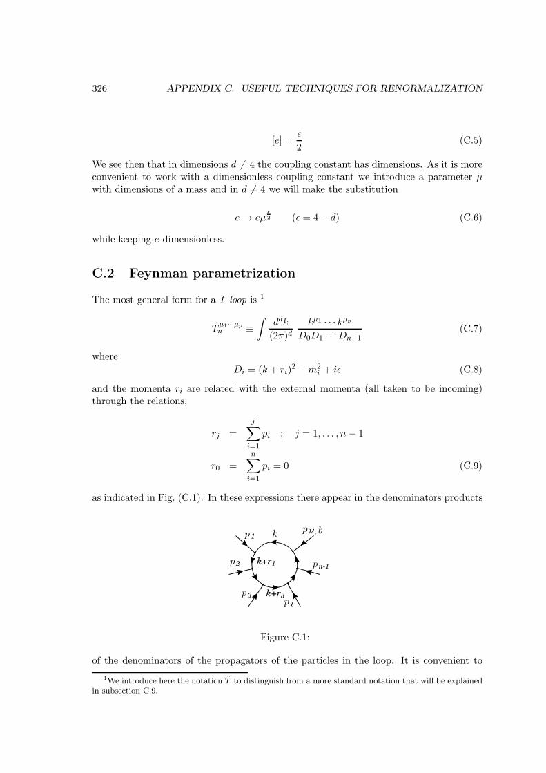
326 APPENDIX C. USEFUL TECHNIQUES FOR RENORMALIZATION
[e] =ǫ
2(C.5)
We see then that in dimensions d 6= 4 the coupling constant has dimensions. As it is moreconvenient to work with a dimensionless coupling constant we introduce a parameter µwith dimensions of a mass and in d 6= 4 we will make the substitution
e→ eµǫ2 (ǫ = 4− d) (C.6)
while keeping e dimensionless.
C.2 Feynman parametrization
The most general form for a 1–loop is 1
Tµ1···µpn ≡
∫ddk
(2π)dkµ1 · · · kµp
D0D1 · · ·Dn−1(C.7)
where
Di = (k + ri)2 −m2
i + iǫ (C.8)
and the momenta ri are related with the external momenta (all taken to be incoming)through the relations,
rj =
j∑
i=1
pi ; j = 1, . . . , n − 1
r0 =
n∑
i=1
pi = 0 (C.9)
as indicated in Fig. (C.1). In these expressions there appear in the denominators products
1
2
3
n-1k+r1
k+r3
ν, b
i
k p
p
pp
p
p
Figure C.1:
of the denominators of the propagators of the particles in the loop. It is convenient to
1We introduce here the notation T to distinguish from a more standard notation that will be explainedin subsection C.9.

C.2. FEYNMAN PARAMETRIZATION 327
combine these products in just one common denominator. This is achieved by a techniquedue to Feynman. Let us exemplify with two denominators.
1
ab=
∫ 1
0
dx
[ax+ b(1− x)]2(C.10)
The proof is trivial. In fact
∫dx
1
[ax+ b(1− x)]2=
x
b [(a− b)x+ b](C.11)
and therefore Eq. (C.10) immediately follows. Taking successive derivatives with respectto a and b we get
1
apbq=
Γ(p+ q)
Γ(p)Γ(q)
∫ 1
0dx
xp−1(1− x)q−1
[ax+ b(1− x)]p+q(C.12)
and using induction we obtain a general formula
1
a1a2 · · · an= Γ(n)
∫ 1
0dx1
∫ 1−x1
0dx2 · · ·
∫ 1−x1−···−xn−2
0
dxn−1[a1x1 + a2x2 + · · ·+ an(1− x1 − · · · − xn−1)]
n (C.13)
Before closing the section let us give an example that will be useful in the self-energy case.Consider the situation with the kinematics described in Fig. (C.2).
p+k
k
pp
Figure C.2:
We get
I =
∫ddk
(2π)d1[
(k + p)2 −m21 + iǫ
] [k2 −m2
2 + iǫ]
=
∫ 1
0dx
∫ddk
(2π)d1
[k2 + 2p · k x+ p2 x−m2
1 x−m22 (1− x) + iǫ
]2
=
∫ 1
0dx
∫ddk
(2π)d1
[k2 + 2P · k −M2 + iǫ]2
328 APPENDIX C. USEFUL TECHNIQUES FOR RENORMALIZATION
=
∫ 1
0dx
∫ddk
(2π)d1
[(k + P )2 − P 2 −M2 + iǫ]2(C.14)
where in the last line we have completed the square in the term with the loop momentak. The quantities P and M2 are, in this case, defined by
P = xp (C.15)
and
M2 = −x p2 +m21 x+m2
2 (1− x) (C.16)
They depend on the masses, external momenta and Feynman parameters, but not in theloop momenta. Now changing variables k → k−P we get rid of the linear terms in k andfinally obtain
I =
∫ 1
0dx
∫ddk
(2π)d1
[k2 − C + iǫ]2(C.17)
where C is independent of the loop momenta k and it is given by
C = P 2 +M2 (C.18)
Notice that the iǫ factors will add correctly and can all be put as in Eq. (C.17).
C.3 Wick Rotation
From the example of the last section we can conclude that all the scalar integrals can bereduced to the form
Ir,m =
∫ddk
(2π)dk2
r
[k2 − C + iǫ]m(C.19)
It is also easy to realize that also all the tensor integrals can be obtained from the scalarintegrals. For instance
∫ddk
(2π)dkµ
[k2 − C + iǫ]m= 0
∫ddk
(2π)dkµkν
[k2 − C + iǫ]m=
1
dgµν
∫ddk
(2π)dk2
[k2 − C + iǫ]m(C.20)
and so on. Therefore the integrals Ir,m are the important quantities to evaluate. We willconsider that C > 0. The case C < 0 can be done by analytical continuation of the finalformula for C > 0.
To evaluate the integral Ir,m we will use integration in the complex plane of the variablek0 as described in Fig. C.3. We can then write
Ir,m =
∫dd−1k(2π)d
∫dk0
k2r
[k20 − |~k|2 − C + iǫ
]m (C.21)

C.4. SCALAR INTEGRALS IN DIMENSIONAL REGULARIZATION 329
x
x
0Re
Im 0k
k
Figure C.3:
The function under the integral has poles for
k0 = ±(√
|~k|2 + C − iǫ
)(C.22)
as shown in Fig. C.3. Using the properties of functions of complex variables (Cauchy the-orem) we can deform the contour, changing the integration from the real to the imaginaryaxis plus the two arcs at infinity. This can be done because in deforming the contour wedo not cross any pole. Notice the importance of the iǫ prescription to be able to do this.The contribution from the arcs at infinity vanishes in dimension sufficiently low for theintegral to converge, as we assume in dimensional regularization. We have then changedthe integration along the real axis into an integration along the imaginary axis in the planeof the complex variable k0. If we write
k0 = ik0E com
∫ +∞
−∞dk0 → i
∫ +∞
−∞dk0E (C.23)
and k2 = (k0)2 − |~k|2 = −(k0E)2 − |~k|2 ≡ −k2E , where kE = (k0E ,
~k) is an euclideanvector. By this we mean that we calculate the scalar product using the euclidean metricdiag(+,+,+,+),
k2E = (k0E)2 + |~k|2 (C.24)
We can them write
Ir,m = i(−1)r−m∫
ddkE(2π)d
k2r
E[k2E + C
]m (C.25)
where we do not need the iǫ because the denominator is strictly positive (C > 0). Thisprocedure is known as Wick Rotation. We note that the Feynman prescription for thepropagators that originated the iǫ rule for the denominators is crucial for the Wick rotationto be possible.
C.4 Scalar integrals in dimensional regularization
We have seen in the last section that the scalar integrals to be calculated with dimensionalregularization had the general form of Eq. (C.25). We are now going to find a general

330 APPENDIX C. USEFUL TECHNIQUES FOR RENORMALIZATION
formula for Ir,m. We begin by writing
∫ddkE =
∫dk k
d−1dΩd−1 (C.26)
where k =√
(k0E)2 + |~k|2 is the length of the vector kE in the euclidean space in d dimen-
sions and dΩd−1 is the solid angle that generalizes spherical coordinates in that euclideanspace. The angles are defined by
kE = k(cos θ1, sin θ1 cos θ2, sin θ1 sin θ2, sin θ1 sin θ2 cos θ3, . . . , sin θ1 · · · sin θd−1) (C.27)
We can then write ∫dΩd−1 =
∫ π
0sin θd−21 dθ1 · · ·
∫ 2π
0dθd−1 (C.28)
Using now ∫ π
0sin θm dθ =
√π
Γ(m+12 )
Γ(m+22 )
(C.29)
where Γ(z) is the gamma function (see section C.6) we get
∫dΩd−1 = 2
πd2
Γ(d2)(C.30)
The integration in k is done using the result
∫ ∞
0dx
xp
(xn + an)q= π(−1)q−1 ap+1−nq Γ(p+1
n )
n sin(π p+1n ) Γ(p+1
2 − q + 1)(C.31)
and we finally get
Ir,m = iCr−m+ d2(−1)r−m
(4π)d2
Γ(r + d2)
Γ(d2)
Γ(m− r − d2)
Γ(m)(C.32)
Before ending the section we note that the integral representation for Ir,m, Eq. (C.19), isvalid only for d < 2(m − r) to ensure convergence when k → ∞. However the final formin Eq. (C.32) can be analytically continued for all values of d except for those where thefunction Γ(m− r − d/2) has poles, that is for (see section C.6),
m− r − d
26= 0,−1,−2, . . . (C.33)
For the application in dimensional regularization it is convenient to rewrite Eq. (C.32)using the relation d = 4− ǫ. we get
Ir,m = i(−1)r−m
(4π)2
(4π
C
) ǫ2
C2+r−m Γ(2 + r − ǫ2)
Γ(2− ǫ2)
Γ(m− r − 2 + ǫ2 )
Γ(m)(C.34)

C.5. TENSOR INTEGRALS IN DIMENSIONAL REGULARIZATION 331
C.5 Tensor integrals in dimensional regularization
We are frequently faced with the task of evaluating the tensor integrals of the form ofEq. (C.7),
Tµ1···µpn ≡
∫ddk
(2π)dkµ1 · · · kµp
D0D1 · · ·Dn−1(C.35)
The first step is to reduce to one common denominator using the Feynman parameteriza-tion technique. The result is,
Tµ1···µpn = Γ(n)
∫ 1
0dx1 · · ·
∫ 1−x1−···−xn−2
0dxn−1
∫ddk
(2π)dkµ1 · · · kµp
[k2 + 2k · P −M2 + iǫ]n
= Γ(n)
∫ 1
0dx1 · · ·
∫ 1−x1−···−xn−2
0dxn−1 I
µ1···µpn (C.36)
where we have defined
Iµ1···µpn ≡
∫ddk
(2π)dkµ1 · · · kµp
[k2 + 2k · P −M2 + iǫ]n(C.37)
that we call, from now on, the tensor integral. In principle all these integrals can bewritten in terms of scalar integrals. It is however convenient to have a general formula forthem. This formula can be obtained by noticing that
∂
∂Pµ1
[k2 + 2k · P −M2 + iǫ]n= −n 2kµ
[k2 + 2k · P −M2 + iǫ]n+1 (C.38)
Using the last equation one can write the final result
Iµ1···µpn =
i
16π2(4π)ǫ/2
Γ(n)
∫ ∞
0
dt
(2t)ptn−3+ǫ/2
∂
∂Pµ1· · · ∂
∂Pµpe−t C (C.39)
where C = P 2 +M2. After doing the derivatives the remaining integrals can be doneusing the properties of the Γ function (see section C.6). Notice that P , M2 and thereforealso C depend not only in the Feynman parameters but also in the exterior momenta.The advantage of having a general formula is that it can be programmed [9] and all theintegrals can then be obtained automatically.
C.6 Γ function and useful relations
The Γ function is defined by the integral
Γ(z) =
∫ ∞
0tz−1e−tdt (C.40)
or equivalently
∫ ∞
0tz−1e−µtdt = µ−zΓ(z) (C.41)

332 APPENDIX C. USEFUL TECHNIQUES FOR RENORMALIZATION
The function Γ(z) has the following important properties
Γ(z + 1) = zΓ(z)
Γ(n+ 1) = n! (C.42)
Another related function is the logarithmic derivative of the Γ function, with the proper-ties,
ψ(z) =d
dzln Γ(z) (C.43)
ψ(1) = −γ (C.44)
ψ(z + 1) = ψ(z) +1
z(C.45)
where γ is the Euler constant. The function Γ(z) has poles for z = 0,−1,−2, · · · . Nearthe pole z = −m we have
Γ(z) =(−1)m
m!
1
m+ z+
(−1)m
m!ψ(m+ 1) +O(z +m) (C.46)
From this we conclude that when ǫ→ 0
Γ( ǫ2
)=
2
ǫ+ ψ(1) +O(ǫ) Γ(−n+ ǫ) =
(−1)n
n!
[2
ǫ+ ψ(n + 1) + 1
](C.47)
and
Γ(1 + ǫ) = 1− γǫ+
(γ2 +
π2
6
)ǫ2
2!+ · · · , ǫ→ 0 (C.48)
Using these results we can expand our integrals in powers of ǫ and separate the divergentand finite parts. For instance for the one of the integrals of the self-energy,
I0,2 =i
(4π)2
(4π
C
) ǫ2 2Γ(1 + ǫ
2)
ǫ
=i
16π2
[2
ǫ− γ + ln 4π − lnC +O(ǫ)
]
=i
16π2[∆ǫ − lnC +O(ǫ)] (C.49)
where we have introduced the notation
∆ǫ =2
ǫ− γ + ln 4π (C.50)
for a combination that will appear in all expressions.

C.7. EXPLICIT FORMULÆ FOR THE 1–LOOP INTEGRALS 333
C.7 Explicit formulæ for the 1–loop integrals
Although we have presented in the previous sections the general formulæ for all the in-tegrals that appear in 1–loop, Eqs. (C.34) and (C.39), in pratice it is convenient to haveexpressions for the most important cases with the expansion on the ǫ already done. Theresults presented below were generated with the Mathematica package OneLoop [9] fromthe general expressions. In these results the integration on the Feynman parameters hasstill to be done. This is in general a difficult problem and we will present in section C.9 analternative way of expressing these integrals more convenient for a numerical evaluation.
C.7.1 Tadpole integrals
With the definitions of Eqs. (C.34) and (C.39) we get
I0,1 =i
16π2C(1 + ∆ǫ − lnC)
Iµ1 = 0
Iµν1 =i
16π21
8C2 gµν(3 + 2∆ǫ − 2 lnC) (C.51)
where for the tadpole integrals
P = 0 ; C = m2 (C.52)
because there are no Feynman parameters and there is only one mass. In this case theabove results are final.
C.7.2 Self–Energy integrals
For the integrals with two denominators we get,
I0,2 =i
16π2(∆ǫ − lnC)
Iµ2 =i
16π2(−∆ǫ + lnC)Pµ
Iµν2 =i
16π21
2
[Cgµν(1 + ∆ǫ − lnC) + 2(∆ǫ − lnC)PµP ν
]
Iµνα2 =i
16π21
2
[− Cgµν(1 + ∆ǫ − lnC)Pα − Cgνα(1 + ∆ǫ − lnC)Pµ
− Cgµα(1 + ∆ǫ − lnC)P ν − (2∆ǫPαPµ − 2 lnCPαPµ)P ν
](C.53)
where, with the notation and conventions of Fig. (C.1), we have
Pµ = x rµ1 ; C = x2 r21 + (1− x)m22 + xm2
1 − x r21 (C.54)

334 APPENDIX C. USEFUL TECHNIQUES FOR RENORMALIZATION
C.7.3 Triangle integrals
For the integrals with three denominators we get,
I0,3 =i
16π2−1
2C
Iµ3 =i
16π21
2CPµ
Iµν3 =i
16π21
4C
[Cgµν(∆ǫ − lnC)− 2PµP ν
]
Iµνα3 =i
16π21
4C
[Cgµν(−∆ǫ + lnC)Pα + Cgνα(−∆ǫ + lnC)Pµ
+ Cgµα(−∆ǫ + lnC)P ν + 2PαPµP ν]
Iµναβ3 =i
16π21
8C
[C2 (1 + ∆ǫ − lnC)
(gµαgνβ + gµβgνα + gαβgµν
)
+ 2C (∆ǫ − lnC)(gµνPαP β + gνβPαPµ + gναP βPµ + gµαP βP ν
+gµβPαP ν + gαβPµP ν)− 4PαP βPµP ν
](C.55)
where
Pµ = x1 rµ1 + x2 r
µ2
C = x21 r21 + x22 r
22 + 2x1 x2 r1 · r2 + x1m
21 + x2m
22
+(1− x1 − x2)m23 − x1 r
21 − x2 r
22 (C.56)
C.7.4 Box integrals
I0,4 =i
16π21
6C2
Iµ4 =i
16π2−1
6C2Pµ
Iµν4 =i
16π2−1
12C2
[Cgµν − 2PµP ν
]
Iµνα4 =i
16π21
12C2
[C (gµνPα + gναPµ + gµαP ν)− 2PαPµP ν
]

C.8. DIVERGENT PART OF 1–LOOP INTEGRALS 335
Iµναβ4 =i
16π21
24C2
[C2 (∆ǫ − lnC)
(gµαgνβ + gµβgνα + gαβgµν
)
− 2C(gµνPαP β + gνβPαPµ + gναP βPµ + gµαP βP ν
+ gµβPαP ν + gαβPµP ν)+ 4PαP βPµP ν
](C.57)
where
Pµ = x1 rµ1 + x2 r
µ2 + x3 r
µ3
C = x21 r21 + x22 r
22 + x23 r
23 + 2x1 x2 r1 · r2 + 2x1 x3 r1 · r3 + 2x2 x3 r2 · r3
+x1m21 + x2m
22 + x3m
23 + (1− x1 − x2 − x3)m
24
−x1 r21 − x2 r22 − x3 r
23 (C.58)
C.8 Divergent part of 1–loop integrals
When we want to study the renomalization of a given theory it is often convenient to haveexpressions for the divergent part of the one-loop integrals, with the integration on theFeynman parameters already done. We present here the results for the most importantcases. These divergent parts were calculated with the help of the package OneLoop [9].The results are for the functions T
µ,µ2,···µnn defined in Eq. (C.35).
C.8.1 Tadpole integrals
Div[T1
]=
i
16π2∆ǫm
2
Div[T µ1
]= 0
Div[T µν1
]=
i
16π21
4∆ǫm
4 gµν (C.59)
C.8.2 Self–Energy integrals
Div[T2
]=
i
16π2∆ǫ
Div[T µ2
]=
i
16π2
(−1
2
)∆ǫ r
µ1
Div[T µν2
]=
i
16π21
12∆ǫ
[(3m2
1 + 3m22 − r21)g
µν + 4rµ1 rν1
]

336 APPENDIX C. USEFUL TECHNIQUES FOR RENORMALIZATION
Div[T µνα2
]=
i
16π2
(− 1
24
)∆ǫ
[(4m2
1 + 2m22 − r21) (g
µνrα1 + gναrµ1 + gµαrν1 )
+ 6 rα1 rµ1 r
ν1
](C.60)
C.8.3 Triangle integrals
Div[T3
]= 0
Div[T µ3
]= 0
Div[T µν3
]=
i
16π21
4∆ǫ g
µν
Div[T µνα3
]=
i
16π2
(− 1
12
)∆ǫ
[gµν(rα1 + rα2 ) + gνα(rµ1 + rµ2 ) + gµα(rν1 + rν2 )
]
Div[T µναβ3
]=
i
16π21
48∆ǫ
[(2m2
1 + 2m22 + 2m2
3)(gµαgνβ + gαβgµν + gµβgνα
)
+gαβ[2rµ1 r
ν1 + rµ1 r
ν2 + (r1 ↔ r2)
]+ gµβ
[2rα1 r
ν1 + rα1 r
ν2 + (r1 ↔ r2)
]
+gνβ[2rα1 r
µ1 + rα1 r
µ2 + (r1 ↔ r2)
]+ gµν
[2rα1 r
β1 + rα1 r
β2 + (r1 ↔ r2)
]
+gµα[2rβ1 r
ν1 + rβ1 r
ν2 + (r1 ↔ r2)
]+ gνα
[2rβ1 r
µ1 + rβ1 r
µ2 + (r1 ↔ r2)
]
+(−r21 + r1 · r2 − r22
) (gµαgνβ + gαβgµν + gµβgνα
)](C.61)
C.8.4 Box integrals
Div[T4
]= Div
[T µ4
]= Div
[T µν4
]= Div
[T µνα4
]= 0
Div[T µναβ4
]=
i
16π21
24∆ǫ
[gµνgαβ + gµβgαν + gµαgνβ
](C.62)
C.9 Passarino-Veltman Integrals
C.9.1 The general definition
The description of the previous sections works well if one just wants to calculate thedivergent part of a diagram or to show the cancellation of divergences in a set of diagrams.If one actually wants to numerically calculate the integrals the task is normally quite

C.9. PASSARINO-VELTMAN INTEGRALS 337
complicated. Except for the self-energy type of diagrams the integration over the Feynmanparameters is normally quite difficult.
To overcome this problem a scheme was first proposed by Passarino and Veltman [10].These scheme with the conventions of [11, 12] was latter implemented in the Mathematicapackage FeynCalc [13] and, for numerical evaluation, in the LoopTools package [14, 15].The numerical evaluation follows the code developed earlier by van Oldenborgh [16].
We will now describe this scheme. We will write the generic one-loop tensor integralas
Tµ1···µpn ≡ (2πµ)4−d
iπ2
∫ddk
kµ1 · · · kµpD0D1D2 · · ·Dn−1
(C.63)
where we follow for the momenta the conventions of section C.2 and Fig. C.1 and definedD0 ≡ Dn and mn = m0 so that D0 = k2 − m2
0 (remember that rn ≡ r0 = 0. Themain difference between this definition and the previous one Eq. (C.7) is that a factor ofi
16π2 is taken out. This is because, as we have seen in section C.3 these integrals alwaysgive that prefactor. So with our new convention that prefactor has to included in theend. Factoring out the i has also the convenience of dealing with real functions in manycases.2 From all those integrals in Eq. (C.63) the scalar integrals are, has we have seen,of particular importance and deserve a special notation. It can be shown that there areonly four independent such integrals, namelly (4− d = ǫ)
A0(m20)=
(2πµ)ǫ
iπ2
∫ddk
1
k2 −m20
(C.64)
B0(r210,m
21,m
22)=
(2πµ)ǫ
iπ2
∫ddk
1∏
i=0
1[(k + ri)2 −m2
i
] (C.65)
C0(r210, r
212, r
220,m
21,m
22,m
23)=
(2πµ)ǫ
iπ2
∫ddk
2∏
i=0
1[(k + ri)2 −m2
i
] (C.66)
D0(r210, r
212, r
223, r
230, r
220, r
213,m
21, . . . ,m
23)=
(2πµ)ǫ
iπ2
∫ddk
3∏
i=0
1[(k + ri)2 −m2
i
] (C.67)
wherer2ij = (ri − rj)
2 ; ∀ i, j = (0, n − 1) (C.68)
Remember that with our conventions r0 = 0 so r2i0 = r2i . In all these expressions the iǫpart of the denominator factors is supressed. The general one-loop tensor integrals are notindependent. Their decomposition is not unique. We follow the conventions of [13, 15] towrite
Bµ ≡ (2πµ)4−d
iπ2
∫ddk kµ
1∏
i=0
1[(k + ri)2 −m2
i
] (C.69)
Bµν ≡ (2πµ)4−d
iπ2
∫ddk kµkν
1∏
i=0
1[(k + ri)2 −m2
i
] (C.70)
2The one loop functions are in general complex, but in some cases they can be real. These casescorrespond to the situation where cutting the diagram does not corresponding to a kinematically allowedprocess.

338 APPENDIX C. USEFUL TECHNIQUES FOR RENORMALIZATION
Cµ ≡ (2πµ)4−d
iπ2
∫ddk kµ
2∏
i=0
1[(k + ri)2 −m2
i
] (C.71)
Cµν ≡ (2πµ)4−d
iπ2
∫ddk kµkν
2∏
i=0
1[(k + ri)2 −m2
i
] (C.72)
Cµνρ ≡ (2πµ)4−d
iπ2
∫ddk kµkνkρ
2∏
i=0
1[(k + ri)2 −m2
i
] (C.73)
Dµ ≡ (2πµ)4−d
iπ2
∫ddk kµ
3∏
i=0
1[(k + ri)2 −m2
i
] (C.74)
Dµν ≡ (2πµ)4−d
iπ2
∫ddk kµkν
3∏
i=0
1[(k + ri)2 −m2
i
] (C.75)
Dµνρ ≡ (2πµ)4−d
iπ2
∫ddk kµkνkρ
3∏
i=0
1[(k + ri)2 −m2
i
] (C.76)
Dµνρσ ≡ (2πµ)4−d
iπ2
∫ddk kµkνkρkσ
3∏
i=0
1[(k + ri)2 −m2
i
] (C.77)
These integrals can be decomposed in terms of (reducible) functions in the following way:
Bµ = rµ1 B1 (C.78)
Bµν = gµν B00 + rµ1 rν1 B11 (C.79)
Cµ = rµ1 C1 + rµ2 C2 (C.80)
Cµν = gµν C00 +
2∑
i=1
rµi rνj Cij (C.81)
Cµνρ =
2∑
i=1
(gµνrρi + gνρrµi + gρµrνi ) C00i +
2∑
i,j,k=1
rµi rνj rρk Cijk (C.82)
Dµ =
3∑
i=1
rµi Di (C.83)
Dµν = gµν D00 +
3∑
i=1
rµi rνj Dij (C.84)
Dµνρ =
3∑
i=1
(gµνrρi + gνρrµi + gρµrνi ) D00i +
2∑
i,j,k=1
rµi rνj rρkDijk (C.85)
Dµνρσ = (gµνgρσ + gµρgνσ + gµσgνρ) D0000
+
3∑
i,j=1
(gµνrρi r
σj + gνρrµi r
σj + gµρrνi r
σj + gµσrνi r
ρj (C.86)
+gνσrµi rρj + gρσrµi r
νj
)D00ij

C.9. PASSARINO-VELTMAN INTEGRALS 339
+
3∑
i,j,k,l=1
rµi rνj rρkrσl Cijkl (C.87)
All coefficient functions have the same arguments as the corresponding scalar functionsand are totally symmetric in their indices. In the FeynCalc [13] package one genericnotation is used,
PaVe[i, j, . . . , r210, r212, . . ., m2
0,m21, . . .
](C.88)
for instanceB11(r
210,m
20,m
21) = PaVe
[1, 1, r210, m2
0,m21]
(C.89)
All these coefficient functions are not independent and can be reduced to the scalar func-tions. FeynCalc provides the command PaVeREduce[...] to acomplish that. This is veryuseful if one wants to check for cancellation of divergences or for gauge invariance wherea number of diagrams have to cancel.
C.9.2 The divergences
The package LoopTools provides ways to numerically check for the cancellation of diver-gences. However it is useful to know the divergent part of the Passarino-Veltman integrals.Only a small number of these integrals are divergent. They are
Div[A0(m
20)]
= ∆ǫm20 (C.90)
Div[B0(r
210,m
20,m
21)]
= ∆ǫ (C.91)
Div[B1(r
210,m
20,m
21)]
= −1
2∆ǫ (C.92)
Div[B00(r
210,m
20,m
21)]
=1
12∆ǫ
(3m2
0 + 3m21 − r210
)(C.93)
Div[B11(r
210,m
20,m
21)]
=1
3∆ǫ (C.94)
Div[C00(r
210, r
212, r
220,m
20,m
21,m
22)]
=1
4∆ǫ (C.95)
Div[C001(r
210, r
212, r
220,m
20,m
21,m
22)]
= − 1
12∆ǫ (C.96)
Div[C002(r
210, r
212, r
220,m
20,m
21,m
22)]
= − 1
12∆ǫ (C.97)
Div[D0000(r
210, . . . ,m
20, . . .)
]=
1
24∆ǫ (C.98)
(C.99)
These results were obtained with the package LoopTools, after reducing to the scalarintegrals with the command PaVeReduce, but they can be verified by comparing with ourresults of section C.8, after factoring out the i/(16π2).
C.9.3 Useful results for PV integrals
Although the PV approach is intended primarily to be used numerically there are situationswhere one wants to have explicit results. These can be useful to check cancellation of
340 APPENDIX C. USEFUL TECHNIQUES FOR RENORMALIZATION
divergences or because in some simple cases the integrals can be done analytically. Wenote that as our conventions for the momenta are the same in sections C.9 and C.7 onecan read immediately the integral representation of the PV in terms of the Feynmanparameters just by comparing both expressions, not forgetting to take out the i/(16π2)factor. For instance, from Eq. (C.81) for Cµν and Eq. (C.55) for Iµν3 we get
C12(r21, r
212, r
22 ,m
20,m
21,m
22) = −Γ(3)
2
4
∫ 1
0dx1
∫ 1−x1
0dx2
x1x2C
(C.100)
with
C = x21 r21 + x22 r
22 + x1 x2 (r
21 + r22 − r212) + x1m
21 + x2m
22
+(1− x1 − x2)m20 − x1 r
21 − x2 r
22 (C.101)
Explicit expression for A0
This integral is trivial. There is no Feynman parameter and the integral can be read fromEq. (C.51). We get, after factoring out the i/(16π2),
A0(m2) = m2
(∆ǫ + 1− ln
m2
µ2
)(C.102)
Explicit expressions for the B functions
Function B0
The general form of the integral B0(p2,m2
1,m22) can be read from Eq. (C.53). We obtain
B0(p2,m2
0,m21) = ∆ǫ −
∫ 1
0dx ln
[−x(1− x)p2 + xm21 + (1− x)m2
0
µ2
](C.103)
From this expression one can easily get the following results,
B0(0,m20,m
21) = ∆ǫ + 1−
m20 ln
m20
µ2−m2
1 lnm2
1µ2
m20 −m2
1
(C.104)
B0(0,m20,m
21) =
A0(m20)−A0(m
21)
m20 −m2
1
(C.105)
B0(0,m2,m2) = ∆ǫ − ln
m2
µ2=A0(m
2)
m2− 1 (C.106)
B0(m2, 0,m2) = ∆ǫ + 2− ln
m2
µ2=A0(m
2)
m2+ 1 (C.107)
B0(0, 0,m2) = ∆ǫ + 1− ln
m2
µ2(C.108)
C.9. PASSARINO-VELTMAN INTEGRALS 341
Function B′0
The derivative of the B0 function with respect to p2 appears many times. From Eq. (C.103)one can derive an integral representation,
B′0(p2,m2
0,m21) = −
∫ 1
0dx
x(1− x)
−p2x(1− x) + xm21 + (1− x)m2
0
(C.109)
An important particular case corresponds to B′0(m2,m2
0,m2) that appears in the self-
energy of the electron. In this case m is the electron mass and m0 = λ is the photon massthat one has to introduce to regularize the IR divergent integral. The integral in this casereduces to
B′0(m2, λ2,m2) = −
∫ 1
0dx
x(1− x)
m2x2 + (1− x)λ2
=1
m2+
1
2m2lnλ2
m2(C.110)
It is clear that in the limit λ→ 0 this integral diverges.
Function B1
The explicit expression can be read from Eq. (C.53). We have
B1(p2,m2
0,m21) = −1
2∆ǫ +
∫ 1
0dxx ln
[−x(1− x)p2 + xm21 + (1− x)m2
0
µ2
](C.111)
For p2 = 0 this integral can be easily evaluated to give
B1(0,m20,m
21) = −1
2∆ǫ +
1
2ln
(m2
0
µ2
)+
−3 + 4t− t2 − 4t ln t+ 2t2 ln t
4(−1 + t)2(C.112)
where we defined
t =m2
1
m20
(C.113)
From Eq. (C.112) one can shown that even for p2 = 0 B1 is not a symmetric function ofthe masses,
B1(p2,m2
0,m21) 6= B1(p
2,m21,m
20) (C.114)
As this might appear strange let us show with one example how the coefficient functionsare tied to our conventions about the order of the momenta and Feynman parameters. Letus consider the contribution to the self-energy of a fermion of mass mf of the exchange ofa scalar with mass ms. We can consider the two choices in Fig. C.4,
Now with the first choice (diagram on the left of Fig. C.4) we have
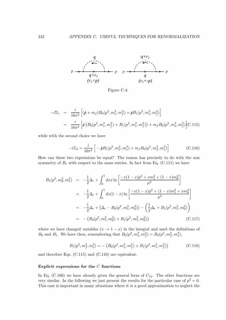
342 APPENDIX C. USEFUL TECHNIQUES FOR RENORMALIZATION
q
q
q+r1
q+r1
(r1=p) (r1=-p)
ppp p
Figure C.4:
−iΣ1 =i
16π2
[(p/+mf )B0(p
2,m2s,m
2f ) + p/B1(p
2,m2s,m
2f )]
=i
16π2
[p/(B0(p
2,m2s,m
2f ) +B1(p
2,m2s,m
2f ))+mfB0(p
2,m2s,m
2f )](C.115)
while with the second choice we have
−iΣ2 =i
16π2
[− p/B1(p
2,m2f ,m
2s) +mfB0(p
2,m2f ,m
2s)]
(C.116)
How can these two expressions be equal? The reason has precisely to do with the nonsymmetry of B1 with respect to the mass entries. In fact from Eq. (C.111) we have
B1(p2,m2
0,m21) = −1
2∆ǫ +
∫ 1
0dxx ln
[−x(1− x)p2 + xm21 + (1− x)m2
0
µ2
]
= −1
2∆ǫ +
∫ 1
0dx(1 − x) ln
[−x(1− x)p2 + (1− x)m21 + xm2
0
µ2
]
= −1
2∆ǫ +
(∆ǫ −B0(p
2,m21,m
20))−(1
2∆ǫ +B1(p
2,m21,m
20)
)
= −(B0(p
2,m21,m
20) +B1(p
2,m21,m
20))
(C.117)
where we have changed variables (x → 1 − x) in the integral and used the definitions ofB0 and B1. We have then, remembering that B0(p
2,m2s,m
2f ) = B0(p
2,m2f ,m
2s),
B1(p2,m2
f ,m2s) = −
(B0(p
2,m2s,m
2f ) +B1(p
2,m2s,m
2f ))
(C.118)
and therefore Eqs. (C.115) and (C.116) are equivalent.
Explicit expressions for the C functions
In Eq. (C.100) we have already given the general form of C12. The other functions arevery similar. In the following we just present the results for the particular case of p2 = 0.This case is important in many situations where it is a good approximation to neglect the

C.9. PASSARINO-VELTMAN INTEGRALS 343
external momenta in comparison with the masses of the particles in the loop. We alsowarn the reader that the coefficient functions Ci, Cij obtained from LoopTools are notwell defined in this limit. Hence there is some utility in given them here.
Function C0
C0(0, 0, 0,m20,m
21,m
22) = −Γ(3)
1
2
∫ 1
0dx1
∫ 1−x1
0dx2
1
x1m21 + x2m
22 + (1− x1 − x2)m
20
= − 1
m20
∫ 1
0dx1
∫ 1−x1
0dx2
1
x1t1 + x2t2 + (1− x1 − x2)
= − 1
m20
−t1 ln t1 + t1t2 ln t1 + t2 ln t2 − t1t2 ln t2(−1 + t1)(t1 − t2)(−1 + t2)
(C.119)
where
t1 =m2
1
m20
; t2 =m2
2
m20
(C.120)
Using the properties of the logarithms one can show that in this limit C0 is a symmetricfunction of the masses. This expression is further simplified when two of the masses areequal, as it happens in the µ→ eγ problem. Then t = t1 = t2,
C0(0, 0, 0,m20,m
21,m
21) = − 1
m20
−1 + t− ln t
(−1 + t)2(C.121)
in agreement with Eq.(20) of [17]. In the case of equal masses for all the loop particles wehave
C0(0, 0, 0,m20,m
20,m
20) = − 1
2m20
(C.122)
Before we close this section on C0 there is another particular case when it is useful to havean explicit case for it. This in the case when it is IR divergent as in the QED vertex. Thefunctions needed is C0(m
2,m2, 0,m2, λ2,m2). Using the definition we have
C0(m2,m2, 0,m2, λ2,m2) = −
∫ 1
0dx1
∫ 1−x1
0dx2
1
m2(1− 2x1 + x21) + x1λ2
= −∫ 1
0dx1
1− x1m2(1− x1)2 + (1− x1)λ2
= −∫ 1
0dx
x
m2x2 + xλ2
=1
2m2lnλ2
m2= B′0(m
2, λ2,m2)− 1
m2(C.123)
Function C00
C00(0, 0, 0,m20,m
21,m
22) = Γ(3)
1
4
∫ 1
0dx1
∫ 1−x1
0dx2
[∆ǫ − ln
(C
µ2
)]
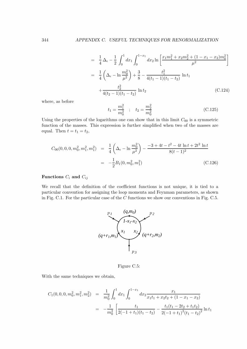
344 APPENDIX C. USEFUL TECHNIQUES FOR RENORMALIZATION
=1
4∆ǫ −
1
2
∫ 1
0dx1
∫ 1−x1
0dx2 ln
[x1m
21 + x2m
22 + (1− x1 − x2)m
20
µ2
]
=1
4
(∆ǫ − ln
m20
µ2
)+
3
8− t21
4(t1 − 1)(t1 − t2)ln t1
+t22
4(t2 − 1)(t1 − t2)ln t2 (C.124)
where, as before
t1 =m2
1
m20
; t2 =m2
2
m20
(C.125)
Using the properties of the logarithms one can show that in this limit C00 is a symmetricfunction of the masses. This expression is further simplified when two of the masses areequal. Then t = t1 = t2,
C00(0, 0, 0,m20,m
21,m
21) =
1
4
(∆ǫ − ln
m20
µ2
)− −3 + 4t− t2 − 4t ln t+ 2t2 ln t
8(t− 1)2
= −1
2B1(0,m
20,m
21) (C.126)
Functions Ci and Cij
We recall that the definition of the coefficient functions is not unique, it is tied to aparticular convention for assigning the loop momenta and Feynman parameters, as shownin Fig. C.1. For the particular case of the C functions we show our conventions in Fig. C.5.
1 2
3
x1 x2
1-x1-x2
(q,m0)
(q+r1,m1) (q+r2,m2)
p
pp
Figure C.5:
With the same techniques we obtain,
C1(0, 0, 0,m20,m
21,m
22) =
1
m20
∫ 1
0dx1
∫ 1−x1
0dx2
x1x1t1 + x2t2 + (1− x1 − x2)
= − 1
m20
[t1
2(−1 + t1)(t1 − t2)− t1(t1 − 2t2 + t1t2)
2(−1 + t1)2(t1 − t2)
2 ln t1

C.9. PASSARINO-VELTMAN INTEGRALS 345
+t2
2 − 2t1t22 + t1
2t22
2(−1 + t1)2(t1 − t2)
2(−1 + t2)ln t2
](C.127)
C2(0, 0, 0,m20,m
21,m
22) =
1
m20
∫ 1
0dx1
∫ 1−x1
0dx2
x2x1t1 + x2t2 + (1− x1 − x2)
= − 1
m20
[− t22(t1 − t2)(−1 + t2)
+ln t1
2(−1 + t1)(−1 + t2)2
+2t1t2 − 2t1
2t2 − t22 + t1
2t22
2(−1 + t1)(t1 − t2)2(−1 + t2)
2 ln
(t1t2
)](C.128)
Cij(0, 0, 0,m20,m
21,m
22) = − 1
m20
∫ 1
0dx1
∫ 1−x1
0dx2
xixjx1t1 + x2t2 + (1− x1 − x2)
(C.129)
where we have not written explicitly the Cij for i, j = 1, 2 because they are rather lengthy.However a simple Fortran program can be developed [9] to calculate all the three pointfunctions in the zero external limit case. This is useful because in this case some ofthe functions from LoopTools will fail. Notice that the Ci and Cij functions are notsymmetric in their arguments. This a consequence of their non-uniqueness, they are tiedto a particular convention. This is very important when ones compares with other results.However using their definition one can get some relations. For instance we can show
C1(0, 0, 0,m20,m
21,m
22) = C1(0, 0, 0,m
22,m
21,m
20) (C.130)
C2(0, 0, 0,m20,m
21,m
22) = −C0(0, 0, 0,m
22,m
21,m
20)− C1(0, 0, 0,m
22,m
21,m
20)
−C2(0, 0, 0,m22,m
21,m
20) (C.131)
In the limit m1 = m2 we get the simple expressions,
C1(0, 0, 0,m20,m
21,m
21) = C2(0, 0, 0,m
20,m
21,m
21)
= − 1
m20
3− 4t+ t2 + 2 ln t
4(−1 + t)3(C.132)
C11(0, 0, 0,m20,m
21,m
21) = C22(0, 0, 0,m
20,m
21,m
21) = 2 C12(0, 0, 0,m
20 ,m
21,m
21)
= − 1
m20
−11 + 18t− 9t2 + 2t3 − 6 ln t
18(−1 + t)4(C.133)
in agreement with Eqs. (21-22) of [17]. The case of masses equal gives
C1(0, 0, 0,m20 ,m
20,m
20) = C2(0, 0, 0,m
20 ,m
20,m
20) =
1
6m20
(C.134)
C11(0, 0, 0,m20 ,m
20,m
20) = C22(0, 0, 0,m
20,m
20,m
20) = − 1
12m20
(C.135)

346 APPENDIX C. USEFUL TECHNIQUES FOR RENORMALIZATION
C12(0, 0, 0,m20,m
20,m
20) = − 1
24m20
(C.136)
The package PVzem
As we said before, in many situations it is a good approximation to neglect the externalmomenta. In this case, the loop functions are easier to evaluate and one approach isfor each problem to evaluate them. However our approach here is more in the directionof automatically evaluating the one-loop amplitudes. If one does that with the use ofFeynCalc, has we have been doing, then the result is given in terms of standard functionsthat can be numerically evaluated with the package LoopTools. However this package hasproblems with this limit. This is because this limit is unphysical. Let us illustrate thispoint calculating the functions C1(m
2, 0, 0,m2S ,m
2F ,m
2F ) and C2(m
2, 0, 0,m2S ,m
2F ,m
2F ) for
mB = 100 GeV, mF = 80 GeV and m2 ranging from 10−6 to 100 GeV. To better illustrateour point we show two plots with different scales on the axis.
100
101
102
2 (GeV)
0.20
0.22
0.24
0.26
0.28
0.30
B
2 C
C1
Ex
C2
Ex
C1
Ap= C
2
Ap
S=100 GeV, m
F=80 GeV
i
µ
µ
µ10
-610
-410
-210
010
2
2 (GeV)
-2.00
0.00
2.00
4.00
B
2 C
C1
Ex
C2
Ex
C1
Ap= C
2
Ap
S=100 GeV, m
F=80 GeV
i
µ
µ
µ
Figure C.6:
In these plots, CExi are the exact Ci functions calculated with LoopTools and CAp
i arethe Ci calculated in the zero momenta limit. We can see that only for external momenta(in this case corresponding to the mass m2) close enough to the masses of the particlesin the loop, the exact result deviates from the approximate one. However for very smallvalues of the external momenta, LoopTools has numerical problems as shown in the rightpanel of Fig. C.6. To overcome this problem I have developed a Fortran package thatevaluates all the C functions in the zero external momenta limit. There are no restrictionson the masses being equal or different and the conventions are the same as in FeynCalc
and LoopTools, for instance,
c12zem(m02,m12,m22) = c0i(cc12, 0, 0, 0,m02,m12,m22) (C.137)
where c0i(cc12, · · · ) is the LoopTools notation and c12zem(· · · ) is the notation of mypackage, called PVzem. It can be obtained from the address indicated in Ref.[9]. The

C.9. PASSARINO-VELTMAN INTEGRALS 347
approximate functions shown in Fig. C.6 were calculated using that package. We includehere the Fortran code used to produce that figure.
*************************************************************
* *
* Program LoopToolsExample *
* *
* This program calculates the values used in the plots *
* of Figure 20. For the exact results the LoopTools *
* package was used. The package PVzem was used for the *
* approximate results. *
* *
* Version of 14/05/2012 *
* *
* Author: Jorge C. Romao *
* e-mail: [email protected] *
*************************************************************

348 APPENDIX C. USEFUL TECHNIQUES FOR RENORMALIZATION
program LoopToolsExample
implicit none
*
* LoopTools has to be used with FORTRAN programs with the
* extension .F in order to have the header file "looptools.h"
* preprocessed. This file includes all the definitions used
* by LoopTools.
*
* Functions c1zem and c2zem are provided by the package PVzem.
*
#include "looptools.h"
integer i
real*8 m2,mF2,mS2,m
real*8 lgmmin,lgmmax,lgm,step
real*8 rc1,rc2
real*8 c1zem,c2zem
mS2=100.d0**2
mF2=80.d0**2
*
* Initialize LoopTools. See the LoopTools manual for further
* details. There you can also learn how to set the scale MU
* and how to handle the UR and IR divergences.
*
call ltini
lgmmax=log10(100.d0)
lgmmin=log10(1.d-6)
step=(lgmmax-lgmmin)/100.d0
lgm=lgmmin-step
open(10,file=’plot.dat’,status=’unknown’)
do i=1,101
lgm=lgm+step
m=10.d0**lgm
m2=m**2

C.9. PASSARINO-VELTMAN INTEGRALS 349
*
* In LoopTools the c0i(...) are complex functions. For the
* kinematics chosen here they are real, so we take the real
* part for comparison.
*
rc1=dble(c0i(cc1,m2,0.d0,0.d0,mS2,mF2,mF2))
rc2=dble(c0i(cc2,m2,0.d0,0.d0,mS2,mF2,mF2))
write(10,100)m,rc1*mS2,rc2*mS2,c1zem(mS2,mF2,mF2)*mS2,
& c2zem(mS2,mF2,mF2)*mS2
enddo
100 format(5(e22.14))
call ltexi
end
************** End of Program LoopToolsExample.F ************
When the above program is compiled, the location of the header file looptools.h
must be known by the compiler. This is best achieved by using a Makefile. We givebelow, as an example, the one that was used with the above program. Depending on theinstallation details of LoopTools the paths might be different.
FC =
LT = /usr/local/lib/LoopTools
FFLAGS = -c -O -I$(LT)/include
LDFLAGS =
LINKER = $(FC)
LIB = -L$(LT)/lib
LIBS = -looptools
.f.o:
$(FC) $(FFLAGS) $*.F
files = LoopToolsExample.o PVzem.o
all: $(files)
$(LINKER) $(LDFLAGS) -o Example $(files) $(LIB) $(LIBS)
Explicit expressions for the D functions
Function D0
The various D functions can be calculated in a similar way. However they are ratherlengthy and have to handled numerically [9]. Here we just give D0 for the equal masses

350 APPENDIX C. USEFUL TECHNIQUES FOR RENORMALIZATION
case.
D0(0, · · · , 0,m2,m2,m2,m2) = Γ(4)1
6
∫ 1
0dx1
∫ 1−x1
0dx2
∫ 1−x1−x2
0dx3
1
(m2)2
=1
m4
∫ 1
0dx1
∫ 1−x1
0dx2
∫ 1−x1−x2
0dx3
=1
6m4(C.138)
C.10 Examples of 1-loop calculations with PV functions
In this section we will work out in detail a few examples of one-loop calculations using theFeynCalc package and the Passarino-Veltman scheme.
C.10.1 Vaccum Polarization in QED
We have done this example in section 4.1.1 using the techniques described in sections C.3,C.4 and C.5. Now we will use FeynCalc. The first step is to write the Matematica
program. We list it below:
(*********************** Program VacPol.m **************************)
(* First input FeynCalc *)
<< FeynCalc.m
(* These are some shorthands for the FeynCalc notation *)
dm[mu_]:=DiracMatrix[mu,Dimension->D]
dm[5]:=DiracMatrix[5]
ds[p_]:=DiracSlash[p]
mt[mu_,nu_]:=MetricTensor[mu,nu]
fv[p_,mu_]:=FourVector[p,mu]
epsilon[a_,b_,c_,d_]:=LeviCivita[a,b,c,d]
id[n_]:=IdentityMatrix[n]
sp[p_,q_]:=ScalarProduct[p,q]
li[mu_]:=LorentzIndex[mu]
L:=dm[7]
R:=dm[6]
(* Now write the numerator of the Feynman diagram. We define the
constant
C=alpha/(4 pi)

C.10. EXAMPLES OF 1-LOOP CALCULATIONS WITH PV FUNCTIONS 351
*)
num:= - C Tr[dm[mu] . (ds[q] + m) . dm[nu] . (ds[q]+ds[k]+m)]
(* Tell FeynCalc to evaluate the integral in dimension D *)
SetOptions[OneLoop,Dimension->D]
(* Define the amplitude *)
amp:=num * FeynAmpDenominator[PropagatorDenominator[q+k,m], \
PropagatorDenominator[q,m]]
(* Calculate the result *)
res:=(-I / Pi^2) OneLoop[q,amp]
(***************** End of Program VacPol.m *********************)
The output from Mathematica is:
2 2 2 2 2 2 2 2 2
Out[4]= (4 C (k + 6 m B0[0, m , m ] - 3 (k + 2 m ) B0[k , m , m ])
2 2
(k g[mu, nu] - k[mu] k[nu])) / (9 k )
Now remembering that,
C =α
4π(C.139)
and
iΠµν(k, ε) = −i k2P TµνΠ(k, ε) (C.140)
we get
Π(k, ε) =α
4π
[−4
9− 8
3
m2
k2B0(0,m
2,m2) +4
3
(1 +
2m2
k2
)B0(k
2,m2,m2)
](C.141)
To obtain the renormalized vacuum polarization one needs to know the value of Π(0, ε).To do that one has to take the limit k → 0 in Eq. (C.141). For that one uses the derivativeof the B0 function
B′0(p2,m2
1,m22) ≡
∂
∂p2B0(p
2,m21,m
22) (C.142)

352 APPENDIX C. USEFUL TECHNIQUES FOR RENORMALIZATION
to obtain
Π(0, ε) =α
4π
[−4
9+
4
3B0(0,m
2,m2) +8
3m2B′0(0,m
2,m2)
](C.143)
Using
B′0(0,m2,m2) =
1
6m2(C.144)
we finally get
Π(0, ε) = −δZ3 =α
4π
[4
3B0(0,m
2,m2)
](C.145)
and the final result for the renormalized vertex is:
ΠR(k) =α
3π
[−1
3+
(1 +
2m2
k2
)(B0(k
2,m2,m2)−B0(0,m2,m2)
)](C.146)
If we want to compare with our earlier analytical results we need to know that
B0(0,m2,m2) = ∆ε − ln
m2
µ2(C.147)
Then Eq. (C.146) reproduces the result of Eq. (4.54). The comparison between Eq. (C.146)and Eq. (4.56) can be done numerically using the package LoopTools[15].
C.10.2 Electron Self-Energy in QED
In this section we repeat the calculation of section 4.1.2 using the Passarino-Veltmanscheme. We start with the Mathematica program,
(********************* Program SelfEnergy.m ***********************)
(* First input FeynCalc *)
<< FeynCalc.m
(* These are some shorthands for the FeynCalc notation *)
dm[mu_]:=DiracMatrix[mu,Dimension->D]
dm[5]:=DiracMatrix[5]
ds[p_]:=DiracSlash[p]
mt[mu_,nu_]:=MetricTensor[mu,nu]
fv[p_,mu_]:=FourVector[p,mu]
epsilon[a_,b_,c_,d_]:=LeviCivita[a,b,c,d]
id[n_]:=IdentityMatrix[n]
sp[p_,q_]:=ScalarProduct[p,q]
li[mu_]:=LorentzIndex[mu]
L:=dm[7]
R:=dm[6]
(* Tell FeynCalc to reduce the result to scalar functions *)

C.10. EXAMPLES OF 1-LOOP CALCULATIONS WITH PV FUNCTIONS 353
SetOptions[B0,B1,B00,B11,BReduce->True]
(* Now write the numerator of the Feynman diagram. We define the
constant
C= - alpha/(4 pi)
The minus sign comes from the photon propagator. The factor
i/(16 pi^2) is already included in this definition.
*)
num:= C dm[mu] . (ds[p]+ds[k]+m) . dm[mu]
(* Tell FeynCalc to evaluate the one-loop integral in dimension D *)
SetOptions[OneLoop,Dimension->D]
(* Define the amplitude *)
amp:= num \
FeynAmpDenominator[PropagatorDenominator[p+k,m], \
PropagatorDenominator[k]]
(* Calculate the result *)
res:=(-I / Pi^2) OneLoop[k,amp]
ans=-res;
(*
The minus sign in ans comes from the fact that -i \Sigma = diagram
*)
(* Calculate the functions A(p^2) and B(p^2) *)
A=Coefficient[ans,DiracSlash[p],0];
B=Coefficient[ans,DiracSlash[p],1];
(* Calculate deltm *)

354 APPENDIX C. USEFUL TECHNIQUES FOR RENORMALIZATION
delm=A + m B /. p->m
(* Calculate delZ2 *)
Ap2 = A /. ScalarProduct[p,p]->p2
Bp2 = B /. ScalarProduct[p,p]->p2
aux=2 m D[Ap2,p2] + Bp2 \
+ 2 m^2 D[Bp2,p2] /. D[B0[p2,0,m^2],p2]->DB0[p2,0,m^2]
aux2= aux /. p2->m^2
aux3= aux2 /. A0[m^2]->m^2 (B0[m^2,0,m^2] -1)
delZ2=Simplify[aux3]
(***************** End of Program SelfEnergy.m ********************)
The output from Mathematica is:
2 2
A = -(C (-2 m + 4 m B0[p , 0, m ]))
2 2 2 2 2 2
C (p + A0[m ] - (m + p ) B0[p , 0, m ])
B = -(-----------------------------------------)
2
p
2 2 2 2 2
C (m - A0[m ] - 2 m B0[m , 0, m ])
delm = ------------------------------------
m
2 2 2 2 2
delZ2= C (-2 + B0[m , 0, m ] - 4 m DB0[m , 0, m ])
We therefore get
A =αm
π
[−1
2+B0(p
2, 0,m2)
](C.148)

C.10. EXAMPLES OF 1-LOOP CALCULATIONS WITH PV FUNCTIONS 355
B =α
4π
[1 +
1
p2A0(m
2)−(1 +
m2
p2
)B0(p
2, 0,m2)
](C.149)
δm =3αm
4π
[−1
3+
1
3m2A0(m
2) +2
3B0(m
2, 0,m2)
](C.150)
One can check that Eq. (C.150) is in agreement with Eq. (4.80). For that one needs thefollowing relations,
A0(m2) = m2
(B0(m
2, 0,m2)− 1)
(C.151)
B0(m2, 0,m2) = ∆ε + 2− ln
m2
µ2(C.152)
∫ 1
0dx(1 + x) ln
m2x2
µ2= −5
2+
3
2lnm2
µ2(C.153)
For δZ2 we get
δZ2 =α
4π
[2−B0(m
2, 0,m2)− 4m2B′0(m2, λ2,m2)
](C.154)
This expression can be shown to be equal to Eq. (4.83) although this is not trivial. Thereason is that B′0 is IR divergent, hence the parameter λ that controls the divergence.
C.10.3 QED Vertex
In this section we repeat the calculation of section 4.1.3 for the QED vertex using thePassarino-Veltman scheme. The Mathematica program should by now be easy to under-stand. We just list it here,
(********************* Program QEDVertex.m ***********************)
(* First input FeynCalc *)
<< FeynCalc.m
(* These are some shorthands for the FeynCalc notation *)
dm[mu_]:=DiracMatrix[mu,Dimension->D]
dm[5]:=DiracMatrix[5]
ds[p_]:=DiracSlash[p]
mt[mu_,nu_]:=MetricTensor[mu,nu]
fv[p_,mu_]:=FourVector[p,mu]
epsilon[a_,b_,c_,d_]:=LeviCivita[a,b,c,d]
id[n_]:=IdentityMatrix[n]
sp[p_,q_]:=ScalarProduct[p,q]
li[mu_]:=LorentzIndex[mu]
L:=dm[7]
R:=dm[6]

356 APPENDIX C. USEFUL TECHNIQUES FOR RENORMALIZATION
(* Tell FeynCalc to reduce the result to scalar functions *)
SetOptions[B1,B00,B11,BReduce->True]
(* Now write the numerator of the Feynman diagram. We define the
constant
C= alpha/(4 pi)
The kinematics is: q = p1 -p2 and the internal momenta is k.
*)
num:=Spinor[p1,m] . dm[ro] . (ds[p1]-ds[k]+m) . ds[a] \
. (ds[p2]-ds[k]+m) . dm[ro] . Spinor[p2,m]
SetOptions[OneLoop,Dimension->D]
amp:=C num \
FeynAmpDenominator[PropagatorDenominator[k,lbd], \
PropagatorDenominator[k-p1,m], \
PropagatorDenominator[k-p2,m]]
(* Define the on-shell kinematics *)
onshell=ScalarProduct[p1,p1]->m^2,ScalarProduct[p2,p2]->m^2, \
ScalarProduct[p1,p2]->m^2-q2/2
(* Define the divergent part of the relevant PV functions*)
div=B0[0,0,m^2]->Div,B0[0,m^2,m^2]->Div, \
B0[m^2,0,m^2]->Div,B0[m^2,lbd^2,m^2]->Div,\
B0[q2,m^2,m^2]->Div,B0[0,lbd^2,m^2]->Div
res1:=(-I / Pi^2) OneLoop[k,amp]
res:=res1 /. onshell
auxV1:= res /.onshell
auxV2:= PaVeReduce[auxV1]
auxV3:= auxV2 /. div
divV:=Simplify[Div*Coefficient[auxV3,Div]]
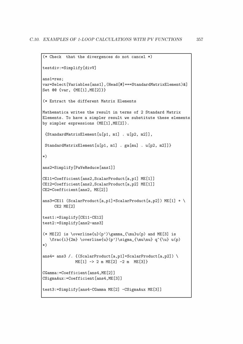
C.10. EXAMPLES OF 1-LOOP CALCULATIONS WITH PV FUNCTIONS 357
(* Check that the divergences do not cancel *)
testdiv:=Simplify[divV]
ans1=res;
var=Select[Variables[ans1],(Head[#]===StandardMatrixElement)&]
Set @@ var, ME[1],ME[2]
(* Extract the different Matrix Elements
Mathematica writes the result in terms of 2 Standard Matrix
Elements. To have a simpler result we substitute these elements
by simpler expressions (ME[1],ME[2]).
StandardMatrixElement[u[p1, m1] . u[p2, m2]],
StandardMatrixElement[u[p1, m1] . ga[mu] . u[p2, m2]]
*)
ans2=Simplify[PaVeReduce[ans1]]
CE11=Coefficient[ans2,ScalarProduct[a,p1] ME[1]]
CE12=Coefficient[ans2,ScalarProduct[a,p2] ME[1]]
CE2=Coefficient[ans2, ME[2]]
ans3=CE11 (ScalarProduct[a,p1]+ScalarProduct[a,p2]) ME[1] + \
CE2 ME[2]
test1:=Simplify[CE11-CE12]
test2:=Simplify[ans2-ans3]
(* ME[2] is \overlineu(p’)\gamma_\muu(p) and ME[3] is
\fraci2m \overlineu(p’)\sigma_\mu\nu q^\u u(p)
*)
ans4= ans3 /. (ScalarProduct[a,p1]+ScalarProduct[a,p2]) \
ME[1] -> 2 m ME[2] -2 m ME[3]
CGamma:=Coefficient[ans4,ME[2]]
CSigmaAux:=Coefficient[ans4,ME[3]]
test3:=Simplify[ans4-CGamma ME[2] -CSigmaAux ME[3]]

358 APPENDIX C. USEFUL TECHNIQUES FOR RENORMALIZATION
F2:=Simplify[CSigmaAux /. lbd->0]
delZ1aux= - CGamma /. q2->0
delZ1:= delZ1aux /. lbd->0
F1:=CGamma + delZ1 /. lbd->0
(***************** End of Program QEDVertex.m ********************)
From this program we can obtain first the value of δZ1. We get
2 2 2 2 2
delZ1= C(1 - B0[0, 0, m ] + 2 B0[0, m , m ] - 2 B0[m , 0, m ] -
2 2 2 2 2
4 m C0[m , m , 0, m , 0, m ])
which can be written as
δZ1 =α
2π
[1−B0(0, 0,m
2) + 2B0(0,m2,m2)− 2B0(m
2,m2)
−4m2C0(m2,m2, 0,m2, λ2,m2)
](C.155)
where we have introduced a small mass for the photon in the function C0(m2,m2, 0,m2, λ2,m2)
because it is IR divergent when λ→ 0 (see Eq. (C.123)). Using the results of Eqs. (C.106),(C.107), (C.108) and Eq. (C.123) we can show the important result
δZ1 = δZ2 (C.156)
where δZ2 was defined in Eq. (C.154). After performing the renormalization the coefficientF1(k
2) is finite and given by
2 2 2
q2 q2 B0[0, 0, m ] 2 q2 B0[0, m , m ]
F1 = C (-(---------) - --------------- + ------------------ -
2 2 2
q2 - 4 m q2 - 4 m q2 - 4 m
2 2 2 2 2 2 2 2
8 m B0[0, m , m ] 3 q2 B0[q2, m , m ] 8 m B0[q2, m , m ]
------------------ - ------------------- + -------------------
2 2 2
q2 - 4 m q2 - 4 m q2 - 4 m

C.10. EXAMPLES OF 1-LOOP CALCULATIONS WITH PV FUNCTIONS 359
2 2 2 2 2 2 2
2 q2 B0[m , 0, m ] 4 q2 m C0[m , m , 0, m , 0, m ]
+ ------------------ - -------------------------------- +
2 2
q2 - 4 m q2 - 4 m
4 2 2 2 2 2 2 2 2 2
16 m C0[m , m , 0, m , 0, m ] 2 q2 C0[m , m , q2, m , 0, m ]
------------------------------ - ------------------------------- +
2 2
q2 - 4 m q2 - 4 m
2 2 2 2 2 4 2 2 2 2
12 q2 m C0[m , m , q2, m , 0, m ] 16 m C0[m , m , q2, m , 0, m ]
---------------------------------- - ------------------------------- )
2 2
q2 - 4 m q2 - 4 m
In[5]:= F1 /. q2->0
Out[5]= 0
while the coefficient F2(q2) does not need renormalization and it is given by,
2 2 2 2 2 2
4 m (1 + B0[0, 0, m ] + B0[q2, m , m ] - 2 B0[m , 0, m ])
F2= C ---------------------------------------------------------
2
q2 - 4 m
and for F2(0) we get
2 2 2 2 2
F2[0]= -(C (1 + B0[0, 0, m ] + B0[0, m , m ] - 2 B0[m , 0, m ]))
Using the results of the Appendix we can show that,
F2(0) =α
2π(C.157)
a well known result, first obtained by Schwinger even before the renormalization programwas fully understood (F2(q
2) is finite).

360 APPENDIX C. USEFUL TECHNIQUES FOR RENORMALIZATION
C.11 Modern techniques in a real problem: µ → eγ
In the previous sections we have redone most of the QED standard textbook examplesusing the PV decomposition and automatic tools. Here we want to present a more complexexample, the calculation of the partial width µ → eγ in an arbitrary theory where thecharged leptons couple to scalars and fermions, charged or neutral. This has been done inRef.[17] for fermions and bosons of arbitrary charge QF and QB, but for simplicity I willconsider here separately the cases of neutral and charged scalars.
C.11.1 Neutral scalar charged fermion loop
We will consider a theory with the following interactions,
AL PL + AR PR BL PL +BR PR
F -
F -
l -
l -
S 0 S 0)i ( i ( )
where F− is a fermion with mass mF and S0 a neutral scalar with mass mS . In factBL,R are not independent of AL,R but it is easier for our programming to consider themcompletely general. The Feynman rule for the coupling of the photon with the lepton is−i eQℓ γµ where e is the positron charge (for an electron Qℓ = −1). ℓ−i can be any of theleptons but we will omit all indices in the program, the lepton being identified by its massand from the assumed kinematics
ℓ2(p2) → ℓ1(p1) + γ(k) (C.158)
The diagrams contributing to the process are given in Fig. C.7,
21 q
D1
D2 D3D4
D5
D6
D7
2 2 11q q
D1 D1
1) 2) 3)
k
k
k
p ppp p p
Figure C.7:
where
D1 = q2 −m2S ; D2 = (p2 + q)2 −m2
F ; D3 = (q + p2− k)2 −m2F(C.159)
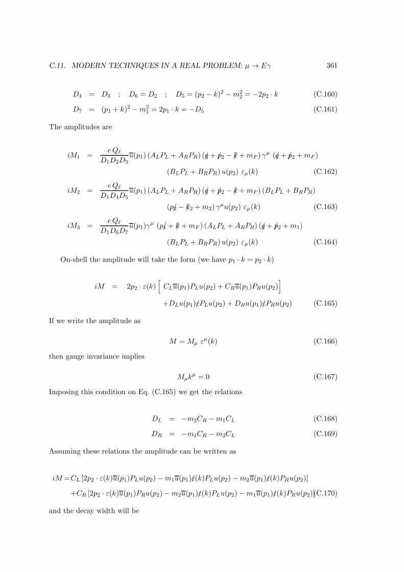
C.11. MODERN TECHNIQUES IN A REAL PROBLEM: µ→ Eγ 361
D4 = D3 ; D6 = D2 ; D5 = (p2 − k)2 −m22 = −2p2 · k (C.160)
D7 = (p1 + k)2 −m21 = 2p1 · k = −D5 (C.161)
The amplitudes are
iM1 =eQℓ
D1D2D3u(p1) (ALPL +ARPR) (q/+ p/2 − k/+mF ) γ
µ (q/+ p/2 +mF )
(BLPL +BRPR)u(p2) εµ(k) (C.162)
iM2 =eQℓ
D1D4D5u(p1) (ALPL +ARPR) (q/+ p/2 − k/+mF ) (BLPL +BRPR)
(p2/− k/2 +m2) γµu(p2) εµ(k) (C.163)
iM3 =eQℓ
D1D6D7u(p1)γ
µ (p1/+ k/+mF ) (ALPL +ARPR) (q/+ p/2 +m1)
(BLPL +BRPR)u(p2) εµ(k) (C.164)
On-shell the amplitude will take the form (we have p1 · k = p2 · k)
iM = 2p2 · ε(k)[CLu(p1)PLu(p2) + CRu(p1)PRu(p2)
]
+DLu(p1)ε/PLu(p2) +DRu(p1)ε/PRu(p2) (C.165)
If we write the amplitude as
M =Mµ εµ(k) (C.166)
then gauge invariance implies
Mµkµ = 0 (C.167)
Imposing this condition on Eq. (C.165) we get the relations
DL = −m2CR −m1CL (C.168)
DR = −m1CR −m2CL (C.169)
Assuming these relations the amplitude can be written as
iM =CL [2p2 · ε(k)u(p1)PLu(p2)−m1u(p1)ε/(k)PLu(p2)−m2u(p1)ε/(k)PRu(p2)]
+CR [2p2 · ε(k)u(p1)PRu(p2)−m2u(p1)ε/(k)PLu(p2)−m1u(p1)ε/(k)PRu(p2)](C.170)
and the decay width will be

362 APPENDIX C. USEFUL TECHNIQUES FOR RENORMALIZATION
Γ =1
16πm32
(m2
2 −m21
)3 (|CL|2 + |CR|2)
(C.171)
As the coefficient of p2 · ε(k) only comes from the 3-point function (amplitude M1) thisjustifies the usual procedure of just calculating that coefficient and forgetting about theself-energies (amplitudes M2 and M3). However these amplitudes are crucial for the can-cellation of divergences and for gauge invariance. Now we will show the power of the auto-matic FeynCalc [13] program and calculate both the coefficients CL,R and DL,R, showingthe cancellation of the divergences and that the relations, Eqs. (C.168) and (C.169) neededfor gauge invariance are satisfied. We start by writing the mathematica program:
(************************ Program mueg-ns.m **************************)
(*
This program calculates the COMPLETE (both the 3 point amplitude and
the two self energy type on each external line) amplitudes for
\mu -> e \gamma when the fermion line in the loop is charged and the
neutral line is a scalar. The \mu has momentum p2 and mass m2, the
electron (p1,m1) and the photon momentum k. The momentum in the loop
is q.
The assumed vertices are,
1) Electron-Scalar-Fermion:
Spinor[p1,m1] (AL P_L + AR P_R) Spinor [pf,mf]
2) Fermion-Scalar-Muon:
Spinor[pf,mf] (BL P_L + BR P_R) Spinor [p2,m2]
*)
dm[mu_]:=DiracMatrix[mu,Dimension->D]
dm[5]:=DiracMatrix[5]
ds[p_]:=DiracSlash[p]
mt[mu_,nu_]:=MetricTensor[mu,nu]
fv[p_,mu_]:=FourVector[p,mu]
epsilon[a_,b_,c_,d_]:=LeviCivita[a,b,c,d]
id[n_]:=IdentityMatrix[n]
sp[p_,q_]:=ScalarProduct[p,q]
li[mu_]:=LorentzIndex[mu]
L:=dm[7]
R:=dm[6]
(*
SetOptions[B0,B1,B00,B11,BReduce->True]
*)

C.11. MODERN TECHNIQUES IN A REAL PROBLEM: µ→ Eγ 363
gA:= AL DiracMatrix[7] + AR DiracMatrix[6]
gB:= BL DiracMatrix[7] + BR DiracMatrix[6]
num1:=Spinor[p1,m1] . gA . (ds[q]+ds[p2]-ds[k]+mf) . ds[Polarization[k]]\
. (ds[q]+ds[p2]+mf) . gB . Spinor[p2,m2]
num2:=Spinor[p1,m1] . gA . (ds[q]+ds[p1]+mf) . gB . (ds[p1]+m2) . \
ds[Polarization[k]] . Spinor[p2,m2]
num3:=Spinor[p1,m1] . ds[Polarization[k]] . (ds[p2]+m1) . gA . \
(ds[q]+ds[p2]+mf) . gB . Spinor[p2,m2]
SetOptions[OneLoop,Dimension->D]
amp1:=num1 \
FeynAmpDenominator[PropagatorDenominator[q+p2-k,mf], \
PropagatorDenominator[q+p2,mf], \
PropagatorDenominator[q,ms]]
amp2:=num2 \
FeynAmpDenominator[PropagatorDenominator[q+p1,mf], \
PropagatorDenominator[p2-k,m2], \
PropagatorDenominator[q,ms]]
amp3:=num3 \
FeynAmpDenominator[PropagatorDenominator[p1+k,m1], \
PropagatorDenominator[q+p2,mf], \
PropagatorDenominator[q,ms]]
(* Define the on-shell kinematics *)
onshell=ScalarProduct[p1,p1]->m1^2,ScalarProduct[p2,p2]->m2^2, \
ScalarProduct[k,k]->0,ScalarProduct[p1,k]->(m2^2-m1^2)/2,\
ScalarProduct[p2,k]->(m2^2-m1^2)/2, \
ScalarProduct[p2,Polarization[k]]->p2epk, \
ScalarProduct[p1,Polarization[k]]->p2epk

364 APPENDIX C. USEFUL TECHNIQUES FOR RENORMALIZATION
(* Define the divergent part of the relevant PV functions*)
div=B0[m1^2,mf^2,ms^2]->Div,B0[m2^2,mf^2,ms^2]->Div, \
B0[0,mf^2,ms^2]->Div,B0[0,mf^2,mf^2]->Div,B0[0,ms^2,ms^2]->Div
res1:=(-I / Pi^2) OneLoop[q,amp1]
res2:=(-I / Pi^2) OneLoop[q,amp2]
res3:=(-I / Pi^2) OneLoop[q,amp3]
res:=res1+res2+res3 /. onshell
auxT1:= res1 /.onshell
auxT2:= PaVeReduce[auxT1]
auxT3:= auxT2 /. div
divT:=Simplify[Div*Coefficient[auxT3,Div]]
auxS1:= res2 + res3 /.onshell
auxS2:= PaVeReduce[auxS1]
auxS3:= auxS2 /. div
divS:=Simplify[Div*Coefficient[auxS3,Div]]
(* Check cancellation of divergences
testdiv should be zero because divT=-divS *)
testdiv:=Simplify[divT + divS]
(* Extract the different Matrix Elements
Mathematica writes the result in terms of 8 Standard Matrix Elements.
To have a simpler result we substitute these elements by simpler
expressions (ME[1],...ME[8]). But they are not all independent. The
final result can just be written in terms of 4 Matrix Elements.
StandardMatrixElement[p2epk u[p1,m1] . ga[6] . u[p2,m2]],
StandardMatrixElement[p2epk u[p1,m1] . ga[7] . u[p2,m2]],
StandardMatrixElement[p2epk u[p1,m1] . gs[k] . ga[6] . u[p2,m2]],
StandardMatrixElement[p2epk u[p1,m1] . gs[k] . ga[7] . u[p2,m2]],
StandardMatrixElement[u[p1,m1] . gs[ep[k]] . ga[6] . u[p2,m2]],
StandardMatrixElement[u[p1,m1] . gs[ep[k]] . ga[7] . u[p2,m2]],
StandardMatrixElement[u[p1,m1] . gs[k] . gs[ep[k]] . ga[6] . u[p2,m2]],
StandardMatrixElement[u[p1,m1] . gs[k] . gs[ep[k]] . ga[7]. u[p2,m2]] *)
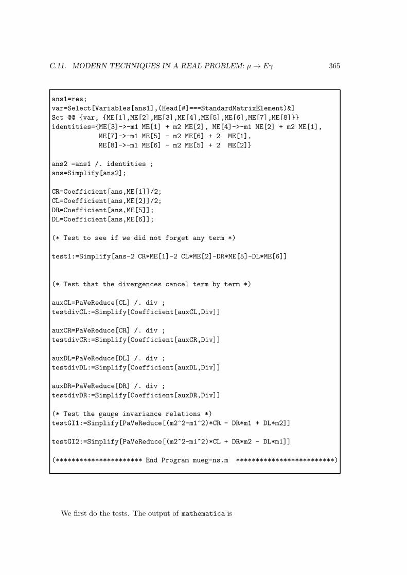
C.11. MODERN TECHNIQUES IN A REAL PROBLEM: µ→ Eγ 365
ans1=res;
var=Select[Variables[ans1],(Head[#]===StandardMatrixElement)&]
Set @@ var, ME[1],ME[2],ME[3],ME[4],ME[5],ME[6],ME[7],ME[8]
identities=ME[3]->-m1 ME[1] + m2 ME[2], ME[4]->-m1 ME[2] + m2 ME[1],
ME[7]->-m1 ME[5] - m2 ME[6] + 2 ME[1],
ME[8]->-m1 ME[6] - m2 ME[5] + 2 ME[2]
ans2 =ans1 /. identities ;
ans=Simplify[ans2];
CR=Coefficient[ans,ME[1]]/2;
CL=Coefficient[ans,ME[2]]/2;
DR=Coefficient[ans,ME[5]];
DL=Coefficient[ans,ME[6]];
(* Test to see if we did not forget any term *)
test1:=Simplify[ans-2 CR*ME[1]-2 CL*ME[2]-DR*ME[5]-DL*ME[6]]
(* Test that the divergences cancel term by term *)
auxCL=PaVeReduce[CL] /. div ;
testdivCL:=Simplify[Coefficient[auxCL,Div]]
auxCR=PaVeReduce[CR] /. div ;
testdivCR:=Simplify[Coefficient[auxCR,Div]]
auxDL=PaVeReduce[DL] /. div ;
testdivDL:=Simplify[Coefficient[auxDL,Div]]
auxDR=PaVeReduce[DR] /. div ;
testdivDR:=Simplify[Coefficient[auxDR,Div]]
(* Test the gauge invariance relations *)
testGI1:=Simplify[PaVeReduce[(m2^2-m1^2)*CR - DR*m1 + DL*m2]]
testGI2:=Simplify[PaVeReduce[(m2^2-m1^2)*CL + DR*m2 - DL*m1]]
(********************** End Program mueg-ns.m *************************)
We first do the tests. The output of mathematica is

366 APPENDIX C. USEFUL TECHNIQUES FOR RENORMALIZATION
(********************** Mathematica output *************************)
In[3]:= << FeynCalc.m
FeynCalc4.1.0.3b Type ?FeynCalc for help or visit
http://www.feyncalc.org
In[4]:= << mueg-ns.m
In[5]:= test1
Out[5]= 0
In[6]:= testdiv
Out[6]= 0
In[7]:= testdivCL
Out[7]= 0
In[8]:= testdivCR
Out[8]= 0
In[9]:= testdivDL
Out[9]= 0
In[10]:= testdivDR
Out[10]= 0
In[11]:= testGI1
Out[11]= 0
In[12]:= testGI2
Out[12]= 0
(******************* End of Mathematica output *********************)
Now we obtain the results for CL

C.11. MODERN TECHNIQUES IN A REAL PROBLEM: µ→ Eγ 367
(********************** Mathematica output *************************)
In[13]:= CL
2 2 2 2 2
Out[13]= (-4 AL BL mf C0[0, m2 , m1 , mf , mf , ms ] +
2 2 2 2 2
4 AL BR m2 PaVe[2, 0, m1 , m2 , mf , mf , ms ] -
2 2 2 2 2
4 AL BL mf PaVe[2, 0, m1 , m2 , mf , mf , ms ] -
2 2 2 2 2
4 AR BL m1 PaVe[1, 2, 0, m1 , m2 , mf , mf , ms ] +
2 2 2 2 2
4 AL BR m2 PaVe[1, 2, 0, m1 , m2 , mf , mf , ms ] +
2 2 2 2 2
4 AL BR m2 PaVe[2, 2, 0, m1 , m2 , mf , mf , ms ]) / 4
and for CR
In[15]:= CR
2 2 2 2 2
Out[15]= (-4 AR BR mf C0[0, m2 , m1 , mf , mf , ms ] +
2 2 2 2 2
4 AR BL m2 PaVe[2, 0, m1 , m2 , mf , mf , ms ] -
2 2 2 2 2
4 AR BR mf PaVe[2, 0, m1 , m2 , mf , mf , ms ] -
2 2 2 2 2
4 AL BR m1 PaVe[1, 2, 0, m1 , m2 , mf , mf , ms ] +
2 2 2 2 2
4 AR BL m2 PaVe[1, 2, 0, m1 , m2 , mf , mf , ms ] +
2 2 2 2 2
4 AR BL m2 PaVe[2, 2, 0, m1 , m2 , mf , mf , ms ]) / 4
(******************* End of Mathematica output **********************)
The expressions for DL,R are quite complicated. They are not normally calculated becausethey can be related to CL,R by gauge invariance. However the power of this automaticprogram can be illustrated by asking for these functions. As they are very long we calculatethem by pieces. We just calculate DL because one can easily check that DR = DL(L ↔ R).

368 APPENDIX C. USEFUL TECHNIQUES FOR RENORMALIZATION
(********************** Mathematica output *************************)
In[12]:= Coefficient[PaVeReduce[DL],AL BL]
2 2 2 2 2 2
m1 mf B0[m1 , mf , ms ] m1 mf B0[m2 , mf , ms ]
Out[12]= ----------------------- - ----------------------- +
2 2 2 2
m1 - m2 m1 - m2
2 2 2 2 2
m1 mf C0[m1 , m2 , 0, mf , ms , mf ]
In[13]:= Coefficient[PaVeReduce[DL],AL BR]
2 2 2 2
(mf - ms ) B0[0, mf , ms ]
Out[13]= --------------------------- -
2 m1 m2
2 2 2 2 2 2
(m1 m2 - m2 mf + m2 ms ) B0[m1 , mf , ms ]
-------------------------------------------- +
2 2
2 m1 (m1 - m2 )
2 2 2 2 2 2
(m1 m2 - m1 mf + m1 ms ) B0[m2 , mf , ms ]
--------------------------------------------
2 2
2 m2 (m1 - m2 )
In[14]:= Coefficient[PaVeReduce[DL],AR BL]
2 2 2 2 2
1 (-2 m1 mf + 2 m1 ms ) B0[m1 , mf , ms ]
Out[14]= - - ---------------------------------------- +
2 2 2
2 m1 (m1 - m2 )
2 2 2 2 2
(-2 m2 mf + 2 m2 ms ) B0[m2 , mf , ms ]
----------------------------------------
2 2
2 m2 (m1 - m2 )

C.11. MODERN TECHNIQUES IN A REAL PROBLEM: µ→ Eγ 369
2 2 2 2 2 2
+ mf C0[m1 , m2 , 0, mf , ms , mf ]
In[15]:= Coefficient[PaVeReduce[DL],AR BR]
2 2 2 2 2 2
m2 mf B0[m1 , mf , ms ] m2 mf B0[m2 , mf , ms ]
Out[15]= ----------------------- - -----------------------
2 2 2 2
m1 - m2 m1 - m2
2 2 2 2 2
+ m2 mf C0[m1 , m2 , 0, mf , ms , mf ]
(******************* End of Mathematica output **********************)
From these expressions one can immediately verify that the divergences cancel in DL,R
and that they are not present in CL,R. To finish this section we just rewrite the CL,R inour usual notation. We get
CL =eQℓ16π2
[ALBLmF
(−C0(0,m
22,m
21,m
2F ,m
2F ,m
2S)− C2(0,m
21,m
22,m
2F ,m
2F ,m
2S))
+ALBRm2
(C2(0,m
21,m
22,m
2F ,m
2F ,m
2S) + C12(0,m
21,m
22,m
2F ,m
2F ,m
2S)
+C22(0,m21,m
22,m
2F ,m
2F ,m
2S))
+ARBLm1C12(0,m21,m
22,m
2F ,m
2F ,m
2S)
](C.172)
CR = CL(L ↔ R) (C.173)
These equations are in agreement with Eqs. (32-34) and Eqs. (38-39) of Ref. [17], althoughsome work has to be done in order to verify that3. This has to do with the fact that thePV decomposition functions are not independent (see the Appendix for further details onthis point). We can however use the power of FeynCalc to verify this. We list below asimple program to accomplish that.
(******************** Program lavoura-ns.m **************************)
(*
This program tests the results of my program mueg-ns.m against the
results obtained by L. Lavoura (hepph/0302221).
*)
(* First load FeynCalc.m and mueg-ns.m *)
3An important difference between our conventions and those of Ref.[17] is that p1 and p2 (and obviouslym1 and m2) are interchanged.

370 APPENDIX C. USEFUL TECHNIQUES FOR RENORMALIZATION
<< FeynCalc.m
<< mueg-ns.m
(*
Now write Lavoura integrals in the notation of FeynCalc. Be careful
with the order of the entries.
*)
c1:=PaVe[1,m2^2,0,m1^2,ms^2,mf^2,mf^2]
c2:=PaVe[2,m2^2,0,m1^2,ms^2,mf^2,mf^2]
d1:=PaVe[1,1,m2^2,0,m1^2,ms^2,mf^2,mf^2]
d2:=PaVe[2,2,m2^2,0,m1^2,ms^2,mf^2,mf^2]
f:=PaVe[1,2,m2^2,0,m1^2,ms^2,mf^2,mf^2]
(* Write Eqs. (32)-(34) of hepph/0302221 in our notation *)
k1:=PaVeReduce[m2*(c1+d1+f)]
k2:=PaVeReduce[m1*(c2+d2+f)]
k3:=PaVeReduce[mf*(c1+c2)]
(*
Now test the results. For this we should use the equivalences:
\rho -> AL BR
\lambda -> AR BL
\xi -> AR BR
\nu -> AL BL
*)
testCLALBR:=Simplify[PaVeReduce[Coefficient[CL, AL BR]-k1]]
testCLARBL:=Simplify[PaVeReduce[Coefficient[CL, AR BL]-k2]]
testCLALBL:=Simplify[PaVeReduce[Coefficient[CL, AL BL]-k3]]
testCRALBR:=Simplify[PaVeReduce[Coefficient[CR, AL BR]-k2]]
testCRARBL:=Simplify[PaVeReduce[Coefficient[CR, AR BL]-k1]]
testCRARBR:=Simplify[PaVeReduce[Coefficient[CR, AR BR]-k3]]
(****************** End of Program lavoura-ns.m **********************)
One can easily check that the output of the six tests is zero, showing the equivalencebetween our results. And all this is done in a few seconds.

C.11. MODERN TECHNIQUES IN A REAL PROBLEM: µ→ Eγ 371
C.11.2 Charged scalar neutral fermion loop
We consider now the case of the scalar being charged and the scalar neutral. The generalcase of both charged [17] can also be easily implemented, but for simplicity we do notconsider it here. The couplings are now
AL PL + AR PR BL PL +BR PR
F 0
F 0
l -
l -
S - S +i ( ) i ( )
and the diagrams contributing to the process are given in Fig. C.8, where all the denomi-
21 q
D1
D4
D5
D6
D7
2 2 11
q
q
D1
1) 2) 3)D’1
D’3 D’2
p
k
k
k
p ppp p p
Figure C.8:
nators are as in Eqs. (C.159)- (C.161) except that
D′1 = q2 −m2F ; D′2 = (q − p1)
2 −m2S ; D′3 = (q − p1 − k)2 −m2
S (C.174)
Also the coupling of the photon to the charged scalar is, in our notation,
−ieQℓ (−2q + p1 + p2)µ (C.175)
The procedure is very similar to the neutral scalar case and we just present here themathematica program and the final result. All the checks of finiteness and gauge invariancecan be done as before.
(************************ Program mueg-cs.m ***************************)
(*
This program calculates the COMPLETE (both the 3 point amplitude and
the two self energy type on each external line) amplitudes for
\mu -> e \gamma when the fermion line in the loop is neutral and the
charged line is a scalar. The \mu has momentum p2 and mass m2, the
electron (p1,m1) and the photon momentum k. The momentum in the loop
is q.

372 APPENDIX C. USEFUL TECHNIQUES FOR RENORMALIZATION
The assumed vertices are,
1) Electron-Scalar-Fermion:
Spinor[p1,m1] (AL P_L + AR P_R) Spinor [pf,mf]
2) Fermion-Scalar-Muon:
Spinor[pf,mf] (BL P_L + BR P_R) Spinor [p2,m2]
*)
dm[mu_]:=DiracMatrix[mu,Dimension->4]
dm[5]:=DiracMatrix[5]
ds[p_]:=DiracSlash[p]
mt[mu_,nu_]:=MetricTensor[mu,nu]
fv[p_,mu_]:=FourVector[p,mu]
epsilon[a_,b_,c_,d_]:=LeviCivita[a,b,c,d]
id[n_]:=IdentityMatrix[n]
sp[p_,q_]:=ScalarProduct[p,q]
li[mu_]:=LorentzIndex[mu]
L:=dm[7]
R:=dm[6]
(*
SetOptions[B0,B1,B00,B11,BReduce->True]
*)
gA:= AL DiracMatrix[7] + AR DiracMatrix[6]
gB:= BL DiracMatrix[7] + BR DiracMatrix[6]
num1:= Spinor[p1,m1] . gA . (ds[q]+mf) . gB . Spinor[p2,m2] \
PolarizationVector[k,mu] ( - 2 fv[q,mu] + fv[p1,mu] + fv[p2,mu] )
num11:=DiracSimplify[num1];
num2:=Spinor[p1,m1] . gA . (ds[q]+ds[p1]+mf) . gB . (ds[p1]+m2) . \
ds[Polarization[k]] . Spinor[p2,m2]
num3:=Spinor[p1,m1] . ds[Polarization[k]] . (ds[p2]+m1) . gA . \
(ds[q]+ds[p2]+mf) . gB . Spinor[p2,m2]
SetOptions[OneLoop,Dimension->D]

C.11. MODERN TECHNIQUES IN A REAL PROBLEM: µ→ Eγ 373
amp1:=num1 \
FeynAmpDenominator[PropagatorDenominator[q,mf],\
PropagatorDenominator[q-p1,ms],\
PropagatorDenominator[q-p1-k,ms]]
amp2:=num2 \
FeynAmpDenominator[PropagatorDenominator[q+p1,mf], \
PropagatorDenominator[p2-k,m2], \
PropagatorDenominator[q,ms]]
amp3:=num3 \
FeynAmpDenominator[PropagatorDenominator[p1+k,m1], \
PropagatorDenominator[q+p2,mf], \
PropagatorDenominator[q,ms]]
(* Define the on-shell kinematics *)
onshell=ScalarProduct[p1,p1]->m1^2,ScalarProduct[p2,p2]->m2^2, \
ScalarProduct[k,k]->0,ScalarProduct[p1,k]->(m2^2-m1^2)/2, \
ScalarProduct[p2,k]->(m2^2-m1^2)/2, \
ScalarProduct[p2,Polarization[k]]->p2epk, \
ScalarProduct[p1,Polarization[k]]->p2epk
(* Define the divergent part of the relevant PV functions*)
div=B0[m1^2,mf^2,ms^2]->Div,B0[m2^2,mf^2,ms^2]->Div, \
B0[0,mf^2,ms^2]->Div,B0[0,mf^2,mf^2]->Div,B0[0,ms^2,ms^2]->Div
res1:=(-I / Pi^2) OneLoop[q,amp1]
res2:=(-I / Pi^2) OneLoop[q,amp2]
res3:=(-I / Pi^2) OneLoop[q,amp3]
res:=res1+res2+res3 /. onshell
auxT1:= res1 /.onshell
auxT2:= PaVeReduce[auxT1]
auxT3:= auxT2 /. div
divT:=Simplify[Div*Coefficient[auxT3,Div]]
auxS1:= res2 + res3 /.onshell
auxS2:= PaVeReduce[auxS1]
auxS3:= auxS2 /. div
divS:=Simplify[Div*Coefficient[auxS3,Div]]

374 APPENDIX C. USEFUL TECHNIQUES FOR RENORMALIZATION
(* Check cancellation of divergences
testdiv should be zero because divT=-divS
*)
testdiv:=Simplify[divT + divS]
(* Extract the different Matrix Elements
Mathematica writes the result in terms of 6 Standard Matrix Elements.
To have a simpler result we substitute these elements by simpler
expressions (ME[1],...ME[6]). Not all are independent.
StandardMatrixElement[p2epk u[p1, m1] . ga[6] . u[p2, m2]],
StandardMatrixElement[p2epk u[p1, m1] . ga[7] . u[p2, m2]],
StandardMatrixElement[p2epk u[p1, m1] . gs[k] . ga[6] . u[p2, m2]],
StandardMatrixElement[p2epk u[p1, m1] . gs[k] . ga[7] . u[p2, m2]],
StandardMatrixElement[u[p1, m1] . gs[ep[k]] . ga[6] . u[p2, m2]],
StandardMatrixElement[u[p1, m1] . gs[ep[k]] . ga[7] . u[p2, m2]]
*)
ans1=res;
var=Select[Variables[ans1],(Head[#]===StandardMatrixElement)&]
Set @@ var, ME[1],ME[2],ME[3],ME[4],ME[5],ME[6]
identities=ME[3]->-m1 ME[1] + m2 ME[2],ME[4]->-m1 ME[2] + m2 ME[1]
ans2 =ans1 /. identities ;
ans=Simplify[ans2];
CR=Coefficient[ans,ME[1]]/2;
CL=Coefficient[ans,ME[2]]/2;
DR=Coefficient[ans,ME[5]];
DL=Coefficient[ans,ME[6]];
(* Test to see if we did not forget any term *)
test1:=Simplify[ans-2*CR*ME[1]-2*CL*ME[2]-DR*ME[5]-DL*ME[6]]

C.11. MODERN TECHNIQUES IN A REAL PROBLEM: µ→ Eγ 375
(* Test that the divergences cancel term by term *)
auxCL:=PaVeReduce[CL] /. div ;
testdivCL:=Simplify[Coefficient[auxCL,Div]]
auxCR:=PaVeReduce[CR] /. div ;
testdivCR:=Simplify[Coefficient[auxCR,Div]]
auxDL:=PaVeReduce[DL] /. div ;
testdivDL:=Simplify[Coefficient[auxDL,Div]]
auxDR:=PaVeReduce[DR] /. div ;
testdivDR:=Simplify[Coefficient[auxDR,Div]]
(* Test the gauge invariance relations *)
testGI1:=PaVeReduce[(m2^2-m1^2)*CR - DR*m1 + DL*m2]
testGI2:=PaVeReduce[(m2^2-m1^2)*CL + DR*m2 - DL*m1]
(********************** End Program mueg-cs.m ***********************)
Note that although these programs look large, in fact they are very simple. Most of it arecomments and tests. The output of this program gives,
(********************* Mathematica output ************************)
In[3]:= CL
2 2 2 2 2
Out[3]= (-2 AR BL m1 C0[0, m1 , m2 , ms , ms , mf ] -
2 2 2 2 2
2 AR BL m1 PaVe[1, m1 , 0, m2 , mf , ms , ms ] -
2 2 2 2 2
4 AR BL m1 PaVe[1, m1 , m2 , 0, ms , mf , ms ] -
2 2 2 2 2
2 AL BL mf PaVe[1, m1 , m2 , 0, ms , mf , ms ] -
2 2 2 2 2
2 AL BR m2 PaVe[2, m1 , 0, m2 , mf , ms , ms ] -
2 2 2 2 2
2 AR BL m1 PaVe[2, m1 , m2 , 0, ms , mf , ms ] +

376 APPENDIX C. USEFUL TECHNIQUES FOR RENORMALIZATION
2 2 2 2 2
2 AL BR m2 PaVe[2, m1 , m2 , 0, ms , mf , ms ] -
2 2 2 2 2
2 AR BL m1 PaVe[1, 1, m1 , m2 , 0, ms , mf , ms ] -
2 2 2 2 2
2 AR BL m1 PaVe[1, 2, m1 , m2 , 0, ms , mf , ms ] +
2 2 2 2 2
2 AL BR m2 PaVe[1, 2, m1 , m2 , 0, ms , mf , ms ]) / 2
(******************* End of Mathematica output ********************)
To finish this section we just rewrite the CL,R in our usual notation. We get
CL =eQℓ16π2
[ALBLmF
(−C1(m
21,m
22, 0,m
2S ,m
2F ,m
2S))
+ALBRm2
(− C2(m
21, 0,m
22,m
2F ,m
2S ,m
2S) + C2(m
21,m
22, 0,m
2S ,m
2F ,m
2S)
+C12(m21,m
22, 0,m
2S ,m
2F ,m
2S))
+ARBLm1
(−C0(0,m
21,m
22,m
2S ,m
2S ,m
2F )− C1(m
21, 0,m
22,m
2F ,m
2S ,m
2S)
−2C1(m21,m
22, 0,m
2S ,m
2F ,m
2S)− C2(m
21,m
22, 0,m
2S ,m
2F ,m
2S)
−C11(m21,m
22, 0,m
2S ,m
2F ,m
2S)−C12(m
21,m
22, 0,m
2S ,m
2F ,m
2S))]
CR = CL(L ↔ R) (C.176)
It is left as an exercise to write a mathematica program that proves that these equationsare in agreement with Eqs. (35-37) and Eqs. (38-39) of Ref. [17].

Appendix D
Feynman Rules for the StandardModel
D.1 Introduction
To do actual calculations it is very important to have all the Feynman rules with consistentconventions. In this Appendix we will give the complete Feynman rules for the StandardModel in the general Rξ gauge.
D.2 The Standard Model
One of the most difficult problems in having a consistent set of of Feynman rules are theconventions. We give here those that are important for building the SM. We will separatethem by gauge group.
D.2.1 Gauge Group SU(3)c
Here the important conventions are for the field strengths and the covariant derivatives.We have
Gaµν = ∂µGaν − ∂νG
aµ + gfabcGbµG
cν , a = 1, . . . , 8 (D.1)
where fabc are the group structure constants, satisfying[T a, T b
]= ifabcT c (D.2)
and T a are the generators of the group. The covariant derivative of a (quark) field q insome representation T a of the gauge group is given by
Dµq =(∂µ − i g GaµT
a)q (D.3)
In QCD the quarks are in the fundamental representation and T a = λa/2 where λa arethe Gell-Mann matrices. A gauge transformation is given by a matrix
U = e−iTaαa (D.4)
377

378 APPENDIX D. FEYNMAN RULES FOR THE STANDARD MODEL
and the fields transform as
q → e−iTaαaq δq = −iT aαaq
GaµTa → UGaµT
aU−1 − i
g∂µUU
−1 δGaµ = −1
g∂µα
a + fabcαbGcµ (D.5)
where the second column is for infinitesimal transformations. With these definitions onecan verify that the covariant derivative transforms like the field itself,
δ(Dµq) = −i T aαa(Dµq) (D.6)
ensuring the gauge invariance of the Lagrangian.
D.2.2 Gauge Group SU(2)L
This is similar to the previous case. We have
W aµν = ∂µW
aν − ∂νW
aµ + gǫabcW b
µWcν , a = 1, . . . , 3 (D.7)
where, for the fundamental representation of SU(2)L we have T a = σa/2 and ǫabc is thecompletely anti-symmetric tensor in 3 dimensions. The covariant derivative for any fieldψL transforming non-trivially under this group is,
DµψL =(∂µ − i g W a
µTa)ψL (D.8)
D.2.3 Gauge Group U(1)Y
In this case the group is abelian and we have
Bµν = ∂µBν − ∂νBµ (D.9)
with the covariant derivative given by
DµψR =(∂µ + i g′ Y Bµ
)ψR (D.10)
where Y is the hypercharge of the field. Notice the different sign convention betweenEq. (D.8) and Eq. (D.9). This is to have the usual definition1
Q = T3 + Y . (D.12)
It is useful to write the covariant derivative in terms of the mass eigenstates Aµ andZµ. These are defined by the relations,
W 3µ = Zµ cos θW −Aµ sin θW
Bµ = Zµ sin θW +Aµ cos θW,
Zµ =W 3
µ cos θW +Bµ sin θW
Aµ = −W 3µ sin θW +Bµ cos θW
. (D.13)
1For this to be consistent one must also have, under hypercharge transformations, for a field of hyper-charge Y ,
ψ′ = e
+iY αY ψ, B′µ = Bµ −
1
g′∂µαY . (D.11)
This is important when finding the ghost interactions. It would have been possible to have a minus signin Eq. (D.10), with a definition θW → θW + π. This would also mean reversing the sign in the exponentof the hypercharge transformation in Eq. (D.11) maintaining the similarity with Eq. (D.5).

D.2. THE STANDARD MODEL 379
Field ℓL ℓR νL uL dL uR dR φ+ φ0
T3 −12 0 1
212 −1
2 0 0 12 −1
2
Y −12 −1 −1
216
16
23 −1
312
12
Q −1 −1 0 23 −1
323 −1
3 1 0
Table D.1: Values of T f3 , Q and Y for the SM particles.
For a field ψL, with hypercharge Y , we get,
DµψL =
[∂µ − i
g√2
(τ+W+
µ + τ−W−µ)− i
g
2τ3W
3µ + ig′Y Bµ
]ψL (D.14)
=
[∂µ − i
g√2
(τ+W+
µ + τ−W−µ)+ ieQAµ − i
g
cos θW
(τ32
−Q sin2 θW
)Zµ
]ψL
where, as usual, τ± = (τ1 ± iτ2)/2 and the charge operator is defined by
Q =
12 + Y 0
0 −12 + Y
, (D.15)
and we have used the relations,
e = g sin θW = g′ cos θW , (D.16)
and the usual definition,
W±µ =W 1µ ∓ iW 2
µ√2
. (D.17)
For a singlet of SU(2)L, ψR we have,
DµψR =[∂µ + ig′Y Bµ
]ψR
=
[∂µ + ieQAµ + i
g
cos θWQ sin2 θWZµ
]ψR . (D.18)
We collect in Table D.1 the quantum number of the SM particles.
D.2.4 The Gauge Field Lagrangian
For completeness we write the gauge field Lagrangian. We have
Lgauge = −1
4GaµνG
aµν − 1
4W aµνW
aµν − 1
4BµνB
µν (D.19)
where the field strengths are given in Eqs. (D.1), and (D.9).

380 APPENDIX D. FEYNMAN RULES FOR THE STANDARD MODEL
D.2.5 The Fermion Fields Lagrangian
Here we give the kinetic part and gauge interaction, leaving the Yukawa interaction for anext section. We have
LFermion =∑
quarks
iqγµDµq +∑
ψL
iψLγµDµψL +
∑
ψR
iψRγµDµψR (D.20)
where the covariant derivatives are obtained with the rules in Eqs. (D.3), (D.14) and(D.18).
D.2.6 The Higgs Lagrangian
In the SM we use an Higgs doublet with the following assignments,
Φ =
φ+
v +H + iϕZ√2
(D.21)
The hypercharge of this doublet is 1/2 and therefore the covariant derivative reads
DµΦ =
[∂µ − i
g√2
(τ+W+
µ + τ−W−µ)− i
g
2τ3W
3µ + i
g′
2Bµ
]Φ (D.22)
=
[∂µ − i
g√2
(τ+W+
µ τ−W−µ
)+ ieQAµ − i
g
cos θW
(τ32
−Q sin2 θW
)Zµ
]Φ
The Higgs Lagrangian is then
LHiggs = (DµΦ)†DµΦ+ µ2Φ†Φ− λ
(Φ†Φ
)2(D.23)
If we expand this Lagrangian we find the following terms
LHiggs = · · ·+ 1
8g2v2W 3
µWµ3 +
1
8g′2v2BµB
µ +1
4gg′v2W 3
µBµ +
1
4g2v2W+
µ W−µ
+1
2v ∂µϕZ
(g′Bµ + gW 3
µ
)+i
2gvW−µ ∂
µϕ+ − i
2gvW+
µ ∂µϕ− (D.24)
The first three terms give, after diagonalization, a massless field, the photon, and a massiveone, the Z, with the relations given in Eq. (D.13), while the fourth gives the mass to thecharged W±µ boson. Using Eq. (D.13) we get,
LHiggs = · · ·+ 1
2M2ZZµZ
µ +M2WW
+µ W
−µ
+MZZµ∂µϕZ + iMW
(W−µ ∂
µϕ+ −W+µ ∂
µϕ−)
(D.25)
where
MW =1
2gv, MZ =
1
cos θW
1
2gv =
1
cos θWMW (D.26)
By looking at Eq. (D.25) we realize that besides finding a realistic spectra for the gaugebosons, we also got a problem. In fact the terms in the last line are quadratic in the fieldsand complicate the definition of the propagators. We now see how one can use the neededgauge fixing to solve also this problem.

D.2. THE STANDARD MODEL 381
D.2.7 The Yukawa Lagrangian
Now we have to spell out the interaction between the fermions and the Higgs doublet thatafter spontaneous symmetry breaking gives masses to the elementary fermions. We have,
LYukawa =− Yl LΦ ℓR − YdQΦ dR − YuQ Φ uR + h.c. (D.27)
where sum is implied over generations, L (Q) are the lepton (quark) doublets and,
Φ = i σ2Φ∗ =
v +H − iϕZ√
2−ϕ−
(D.28)
D.2.8 The Gauge Fixing
As it is well known, we have to gauge fix the gauge part of the Lagrangian to be able todefine the propagators. We will use a generalization of the class of Lorenz gauges, theso-called Rξ gauges. With this choice the gauge fixing Lagrangian reads
LGF = − 1
2ξF 2G − 1
2ξF 2A − 1
2ξF 2Z − 1
ξF−F+ (D.29)
where
F aG =∂µGaµ, FA = ∂µAµ, FZ = ∂µZµ − ξMZϕZ
F+ =∂µW+µ − iξMWϕ
+, F− = ∂µW−µ + iξMWϕ− (D.30)
One can easily verify that with these definitions we cancel the quadratic terms in Eq. (D.25).
D.2.9 The Ghost Lagrangian
The last piece in writing the SM Lagrangian is the ghost Lagrangian. As it is well known,this is given by the Fadeev-Popov prescription,
LGhost =4∑
i=1
[c+∂(δF+)
∂αi+ c−
∂(δF+)
∂αi+ cZ
∂(δFZ )
∂αi+ cA
∂(δFA)
∂αi
]ci
+8∑
a,b=1
ωa∂(δF aG)
∂βbωb (D.31)
where we have denoted by ωa the ghosts associated with the SU(3)c transformationsdefined by,
U = e−iTaβa , a = 1, . . . , 8 (D.32)
and by c±, cA, cZ the electroweak ghosts associated with the gauge transformations,
U = e−iTaαa , a = 1, . . . , 3, U = eiY α
4(D.33)

382 APPENDIX D. FEYNMAN RULES FOR THE STANDARD MODEL
For completeness we write here the gauge transformations of the gauge fixing terms neededto find the Lagrangian in Eq. (D.31). It is convenient to redefine the parameters as
α± =α1 ∓ α2
√2
αZ =α3 cos θW + α4 sin θW
αA =− α3 sin θW + α4 cos θW (D.34)
We then get
δF aG =− ∂µβa + gsf
abcβbGcµ
δFA =− ∂µαA
δFZ =∂µ(δZµ)−MZδϕZ
δF+ =∂µ(δW+µ )− iMW δϕ
+
δF− =∂µ(δW−µ ) + iMW δϕ
− (D.35)
Using the explicit form of the gauge transformations we can finally find the missing pieces,
δZµ =− ∂µαZ + ig cos θW(W+µ α− −W−µ α
+)
(D.36)
δW+µ =− ∂µα
+ + ig[α+ (Zµ cos θW −Aµ sin θw)− (αZ cos θw − αA sin θW )W+
µ
]
δW−µ =− ∂µα− − ig
[α− (Zµ cos θW −Aµ sin θw)− (αZ cos θw − αA sin θW )W−µ
]
and
δϕZ =− 1
2g(α−ϕ+ + α+ϕ−
)+
g
2 cos θWαZ(v +H)
δϕ+ =− ig
2(v +H + iϕZ)α
+ − ig
2
cos 2θWcos θW
ϕ+αZ + ie ϕ+αA
δϕ− =ig
2(v +H − iϕZ)α
− + ig
2
cos 2θWcos θW
ϕ−αZ − ie ϕ−αA (D.37)
D.2.10 The Complete SM Lagrangian
Finally the complete Lagrangian for the Standard Model is obtained putting together allthe pieces. We have,
LSM = Lgauge + LFermion + LHiggs + LYukawa + LGF + LGhost (D.38)
where the different terms were given in Eqs. (D.19), (D.20), (D.23), (D.27), (D.29), (D.31).
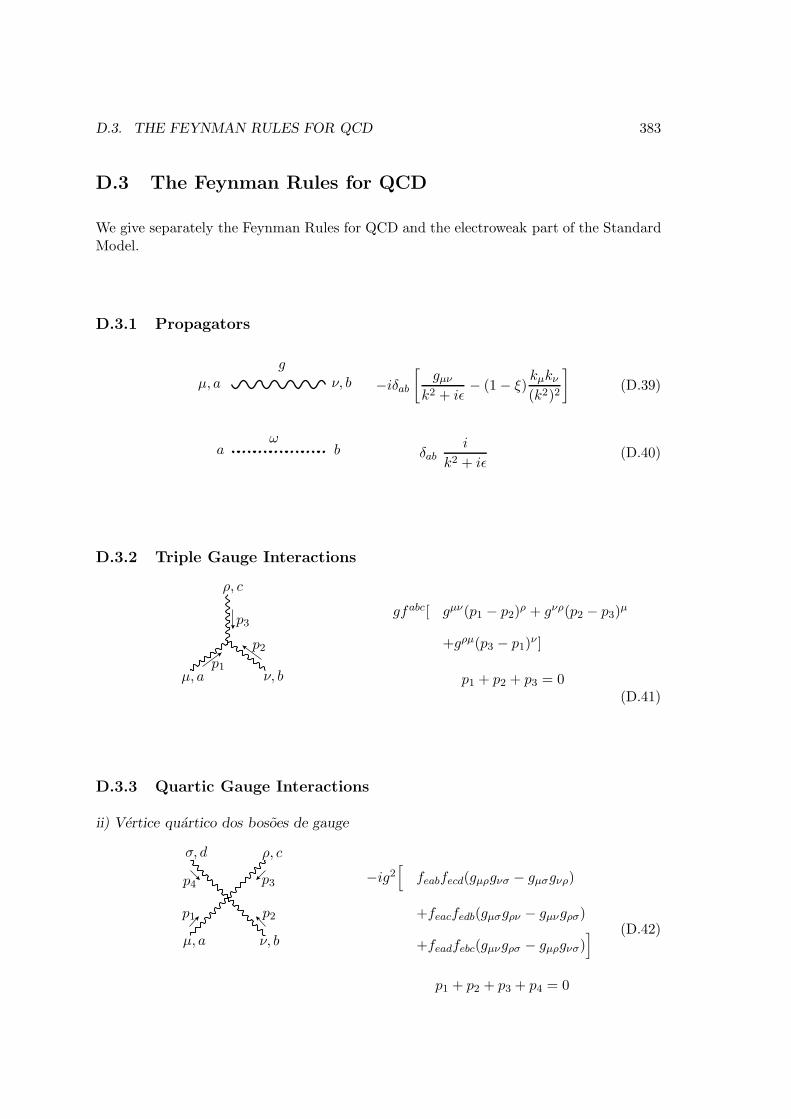
D.3. THE FEYNMAN RULES FOR QCD 383
D.3 The Feynman Rules for QCD
We give separately the Feynman Rules for QCD and the electroweak part of the StandardModel.
D.3.1 Propagators
−iδab[
gµνk2 + iǫ
− (1− ξ)kµkν(k2)2
](D.39)µ, a ν, b
g
δabi
k2 + iǫ(D.40)
ωa b
D.3.2 Triple Gauge Interactions
gfabc[ gµν(p1 − p2)ρ + gνρ(p2 − p3)
µ
+gρµ(p3 − p1)ν ]
p1 + p2 + p3 = 0(D.41)
µ, a ν, b
ρ, c
p1
p2
p3
D.3.3 Quartic Gauge Interactions
ii) Vertice quartico dos bosoes de gauge
−ig2[
feabfecd(gµρgνσ − gµσgνρ)
+feacfedb(gµσgρν − gµνgρσ)
+feadfebc(gµνgρσ − gµρgνσ)]
p1 + p2 + p3 + p4 = 0
(D.42)µ, a ν, b
ρ, cσ, d
p1 p2
p3p4

384 APPENDIX D. FEYNMAN RULES FOR THE STANDARD MODEL
D.3.4 Fermion Gauge Interactions
ig(γµ)βαTaij (D.43)
µ, a
α, jβ, ip1
p2
p3
D.3.5 Ghost Interactions
g Cabcpµ1
p1 +p2 + p3 = 0(D.44)
µ, c
a bp1
p2
p3
D.4 The Feynman Rules for the Electroweak Theory
D.4.1 Propagators
−i[
gµνk2 + iǫ
− (1− ξ)kµkν(k2)2
](D.45)µ ν
γ
−igµνk2 −M2
W + iǫ(D.46)µ ν
W
−igµνk2 −M2
Z + iǫ(D.47)µ ν
Z
i(p/+mf )
p2 −m2f + iǫ
(D.48)p
i
p2 −M2h + iǫ
(D.49)p
h
i
p2 − ξm2Z + iǫ
(D.50)p
ϕZ

D.4. THE FEYNMAN RULES FOR THE ELECTROWEAK THEORY 385
i
p2 − ξm2W + iǫ
(D.51)p
ϕ±
D.4.2 Triple Gauge Interactions
−ie [gαβ(p − k)µ + gβµ(k − q)α + gµα(q − p)β] (D.52)p q
k
W−α
W+β
Aµ
ig cos θW [gαβ(p − k)µ + gβµ(k − q)α + gµα(q − p)β] (D.53)p q
k
W−α
W+β
Zµ
D.4.3 Quartic Gauge Interactions
−ie2 [2gαβgµµ − gαµgβν − gανgβµ] (D.54)
W+α
Aµ
W−β
Aν
−ig2 cos2 θW [2gαβgµν − gαµgβν − gανgβµ] (D.55)
W+α
Zµ
W−β
Zν
ieg cos θW [2gαβgµν − gαµgβν − gανgβµ] (D.56)
W+α
Aµ
W−β
Zν
ig2 [2gαµgβν − gαβgµν − gανgβµ] (D.57)

386 APPENDIX D. FEYNMAN RULES FOR THE STANDARD MODELW+α W−β
W+µ W−ν
D.4.4 Charged Current Interaction
ig√2γµ
1− γ52
(D.58)
ψd,u
ψu,dW±µ
D.4.5 Neutral Current Interaction
(D.59)
ψf
ψf
ψf
ψf
Zµ Aµi
g
cos θWγµ
(gfV − gfAγ5
)−ieQfγµ
where
gfV =1
2T 3f −Qf sin
2 θW , gfA =1
2T 3f . (D.60)
D.4.6 Fermion-Higgs and Fermion-Goldstone Interactions
−i g2
mf
mW(D.61)
h
f
f
−g T 3f
mf
mWγ5 (D.62)
ϕZ
f
f
ig√2
(mu
mWPR,L − md
mWPL,R
)(D.63)
ϕ∓
ψd,u
ψu,d

D.4. THE FEYNMAN RULES FOR THE ELECTROWEAK THEORY 387
D.4.7 Triple Higgs-Gauge and Goldstone-Gauge Interactions
−i e (p+ − p−)µ (D.64)
d
Aµ
ϕ+
ϕ−p−
p+
i gcos 2θW2 cos θW
(p+ − p−)µ (D.65)
p2
Zµ
ϕ+
ϕ−p−
p+
∓ i
2g (k − p)µ (D.66)
p
W±µ
h
ϕ∓k
p
g
2(k − p)µ (D.67)
, b
W±µ
ϕZ
ϕ∓k
p
g
2 cos θ(k − p)µ (D.68)Zµ
h
ϕZ
k
p
−iemW gµν (D.69)
Aµ
W±ν
ϕ∓

388 APPENDIX D. FEYNMAN RULES FOR THE STANDARD MODEL
−ig mZ sin2 θW gµν (D.70)
Zµ
W±ν
ϕ∓
ig mW gµν (D.71)W±µ
W∓ν
h
ig
cos θWmZ gµν (D.72)
Zµ
Zν
h
D.4.8 Quartic Higgs-Gauge and Goldstone-Gauge Interactions
i
2g2 gµν (D.73)
h
h
W±µ
W∓ν
i
2g2 gµν (D.74)
ϕZ
ϕZ
W±µ
W∓ν
i
2
g2
cos2 θWgµν (D.75)
h
h
Zµ
Zν

D.4. THE FEYNMAN RULES FOR THE ELECTROWEAK THEORY 389
i
2
g2
cos2 θWgµν (D.76)
f
ϕZ
ϕZ
Zµ
Zν
2i e2 gµν (D.77)
p
ϕ+
ϕ−
Aµ
Aν
i
2
(g cos 2θWcos θW
)2
gµν (D.78)
p1
ϕ+
ϕ−
Zµ
Zν
i
2g2 gµν (D.79)
ρ, c
ϕ+
ϕ−
W+µ
W−ν
−i g2 sin2 θW2 cos θW
gµν (D.80)
b
ϕ∓
h
W±µ
Zν
∓ g2sin2 θW2 cos θW
gµν (D.81)
ϕ±
ϕZ
W∓µ
Zν
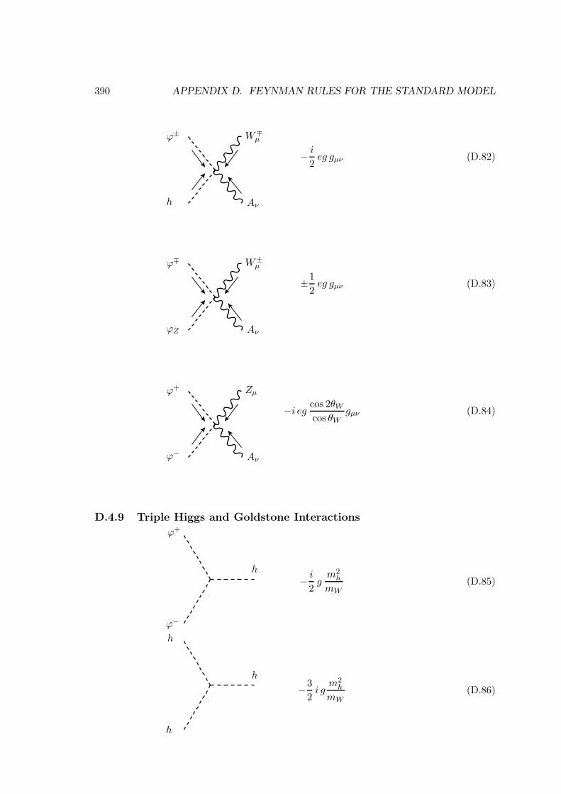
390 APPENDIX D. FEYNMAN RULES FOR THE STANDARD MODEL
− i
2eg gµν (D.82)
ϕ±
h
W∓µ
Aν
±1
2eg gµν (D.83)
ϕ∓
ϕZ
W±µ
Aν
−i eg cos 2θWcos θW
gµν (D.84)
ϕ+
ϕ−
Zµ
Aν
D.4.9 Triple Higgs and Goldstone Interactions
− i
2gm2h
mW(D.85)
ϕ−
ϕ+
h
−3
2i g
m2h
mW(D.86)
h
h
h

D.4. THE FEYNMAN RULES FOR THE ELECTROWEAK THEORY 391
− i
2gm2h
mW(D.87)
f
ϕZ
ϕZ
h
D.4.10 Quartic Higgs and Goldstone Interactions
− i
2g2
m2h
m2W
(D.88)
b
ϕ+
ϕ+
ϕ−
ϕ−
− i
4g2
m2h
m2W
(D.89)
ρ, c
ϕ+
ϕ−
h
h
− i
4g2
m2h
m2W
(D.90)
µ, a
ϕ+
ϕ−
ϕZ
ϕZ
−3
4i g2
m2h
m2W
(D.91)
a
h
h
h
h
− i
4g2m2h
m2W
(D.92)

392 APPENDIX D. FEYNMAN RULES FOR THE STANDARD MODELϕZ
ϕZ
h
h
−3
4i g2
m2h
m2W
(D.93)
ϕZ
ϕZ
ϕZ
ϕZ
D.4.11 Ghost Propagators
i
k2 + iǫ(D.94)
cA
i
k2 − ξm2W + iǫ
(D.95)c±
i
k2 − ξm2Z + iǫ
(D.96)cZ
D.4.12 Ghost Gauge Interactions
∓ie pµ (D.97)Aµ
c±
c±p
±ig cos θW pµ (D.98)Zµ
c±
c±p
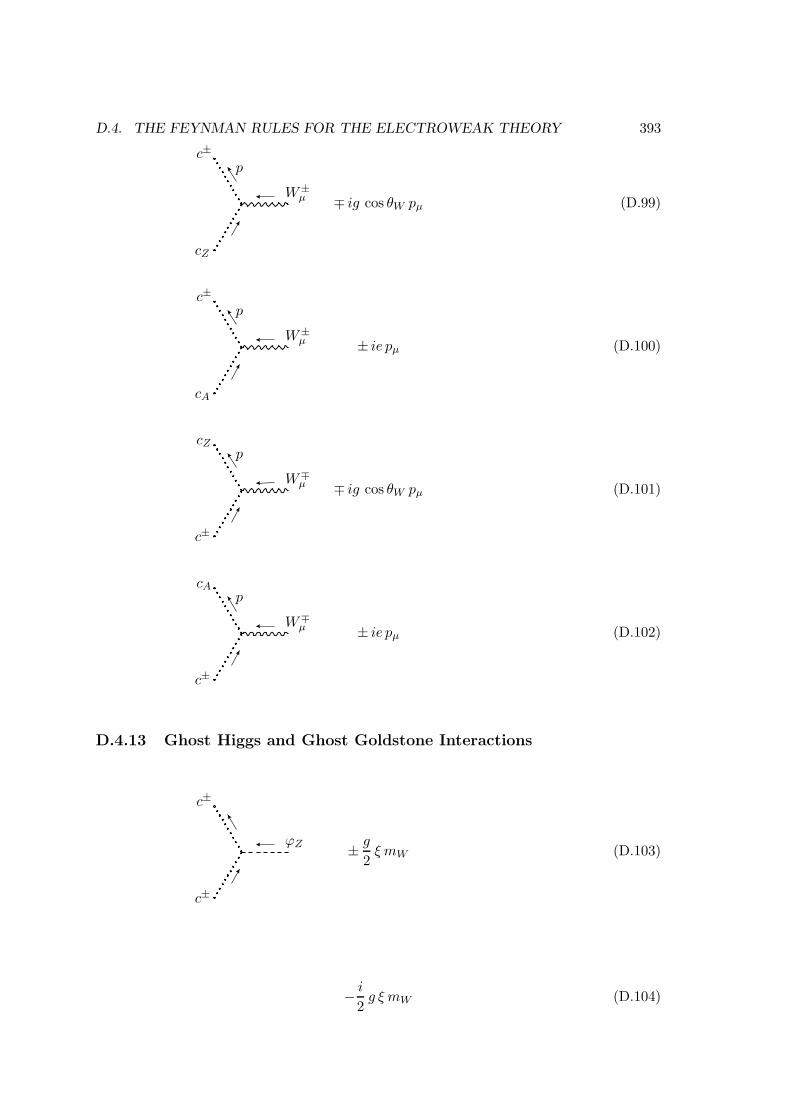
D.4. THE FEYNMAN RULES FOR THE ELECTROWEAK THEORY 393
∓ ig cos θW pµ (D.99)W±µ
c±
cZ
p
± ie pµ (D.100)
µ, a
W±µ
c±
cA
p
∓ ig cos θW pµ (D.101)
p
W∓µ
c±
cZp
± ie pµ (D.102)
p
W∓µ
c±
cAp
D.4.13 Ghost Higgs and Ghost Goldstone Interactions
± g
2ξ mW (D.103)
ϕZ
c±
c±
− i
2g ξ mW (D.104)

394 APPENDIX D. FEYNMAN RULES FOR THE STANDARD MODEL
h
c±
c±
− ig
2 cos θWξ mZ (D.105)
h
cZ
cZ
i
2g ξ mZ (D.106)
ϕ∓
c±
cZ
−ig cos 2θW2 cos θW
ξ mW (D.107)ϕ±
c±
cZ
ie ξ mW (D.108)ϕ±
c±
cA

Bibliography
[1] J. Bjorken and S. Drell, Relativistic Quantum Mechanics (McGraw-Hill, New York,1962).
[2] S. N. Gupta, Proc. Phys. Soc. 63, 681 (1950).
[3] K. Bleuler, Helv. Phys. Acta 23, 567 (1950).
[4] S. S. Schweber, An Introduction to Relativistic Quantum Field Theory (Dover Pub-lications, 1962).
[5] J. C. Romao, Introducao a Teoria do Campo (IST, 2016), Available online athttp://porthos.ist.utl.pt/ftp/textos/itc.pdf.
[6] J. D. Bjorken and S. D. Drell, Relativistic Quantum Fields (McGraw-Hill, N.Y.,1964).
[7] C. Itzykson and J. B. Zuber, Quantum Field Theory (McGraw-Hill, New York, 1980).
[8] H. Lehmann, K. Symanzik and W. Zimmerman, Nuovo Cimento 1, 2005 (1955).
[9] J. C. Romao, Utilities for One Loop Calculations (IST, 2004), Available online athttp://porthos.ist.utl.pt/OneLoop/.
[10] G. Passarino and M. J. G. Veltman, Nucl. Phys. B160, 151 (1979).
[11] A. Denner, Fortschr. Phys. 41, 307 (1993).
[12] R. Mertig, M. Bohm and A. Denner, Comput. Phys. Commun. 64, 345 (1991).
[13] R. Mertig, http://www.feyncalc.org .
[14] T. Hahn and M. Perez-Victoria, Comput. Phys. Commun. 118, 153 (1999), [hep-ph/9807565].
[15] T. Hahn, http://www.feynarts.de/looptools .
[16] G. J. van Oldenborgh, Comput. Phys. Commun. 66, 1 (1991).
[17] L. Lavoura, Eur. Phys. J. C29, 191 (2003), [hep-ph/0302221].
395


![digituma.uma.pt...Blanchard et al. [BSST93], pages 174-187. K. Symanzik. Euclidean Quantum Field Theory. In Local Quan- turn Theory. Academic New York, 1969. S. R. S. Varadhan. Appendix](https://img.pdfslide.us/doc/110x75/6076fa6c4b984871be754bf9/-blanchard-et-al-bsst93-pages-174-187-k-symanzik-euclidean-quantum-field.jpg)