At

Ra

b

a

ARRAA

KDADTMD

1

itwfptm

wegebcaarl

k

h0

Computers and Chemical Engineering 71 (2014) 467–477

Contents lists available at ScienceDirect

Computers and Chemical Engineering

j ourna l ho me pa g e: www.elsev ier .com/ locate /compchemeng

n adaptive moving grid method for solving convection dominatedransport equations in chemical engineering

. Kellinga,∗, J. Bickela, U. Niekena, P.A. Zegelingb

Institute of Chemical Process Engineering, Boeblinger Str. 78, 70199 Stuttgart, GermanyDepartment of Mathematics, P.O. Box 80010, 3508 TA Utrecht, The Netherlands

r t i c l e i n f o

rticle history:eceived 19 May 2014eceived in revised form 5 September 2014ccepted 12 September 2014vailable online 22 September 2014

a b s t r a c t

Convection dominated processes in chemical engineering are frequently accompanied by steep prop-agating fronts. Numerical simulation of corresponding models with uniform fixed grids requires anexcessive amount of grid points along the expected range of the front movement. In this contribution theimplementation of an efficient adaptive grid method is presented and applied to two relevant spatiallyone-dimensional cases, the chlorination stage of the Deacon process and oxygen storage processes in

eywords:ynamic simulationdaptive grideacon processhree-way catalystATLAB

a three-way catalyst. The algorithm exhibits a high accuracy with a much lower number of grid pointsand a therefore reduced computational effort as opposed to a fixed grid simulation. The present workdemonstrates that the algorithm allows for a robust, simple, and fast implementation of the adaptivegrid method in common simulation tools and, together with adequate supplementary material, aims tomake the method readily accessible to the interested reader.

© 2014 Elsevier Ltd. All rights reserved.

IANA

. Introduction

Many convection dominated processes in chemical engineer-ng, especially industrial scale applications, are characterized byhe formation of steep moving fronts (Eigenberger et al., 2007). Aell-known example is the propagation of a thermal and a reaction

ront during an endothermic or exothermic reaction in a tubularacked bed. Traveling fronts are common phenomena in adsorp-ion columns, ion exchangers, regenerative heat exchangers, or

embrane reactors.The numerical simulation of steep moving fronts or shock fronts

ith adequate accuracy in time and space is computationallyxpensive. Many adaptive methods are available to rearrange therid points according to the local errors of the partial differentialquations describing such systems. This allows reducing the num-er of grid points and therefore the number of equations and theomputational cost. Desirable requirements for such methods are

straightforward and easy adaptation of the adaptive grid to the

ctual physical problem and a fast implementation of the algo-ithm in common simulation tools. The method has to find highocal gradients automatically without an a priori specification of

∗ Corresponding author. Tel.: +49 711 685 85247.E-mail addresses: rene.kelling@icvt.uni-stuttgart.de,

elling.rene@googlemail.com (R. Kelling).

ttp://dx.doi.org/10.1016/j.compchemeng.2014.09.011098-1354/© 2014 Elsevier Ltd. All rights reserved.

their temporal position, using general grid defining parameters. Inthis paper we present such a technique using the adaptive gridmethod as developed in Zegeling (2007) and van Dam and Zegeling(2010) for two typical, spatially one-dimensional models of chem-ical engineering applications. The models are solved on a movinggrid by established simulation tools (MATLAB©, DIANA (Krasnyket al., 2006)) which provide efficient and robust solvers.

In Section 2 we classify the presented adaptive grid method anddescribe the main steps of implementation for a general model. InSection 3 the adaptive grid is used to simulate the chlorination stageof the Deacon process. Here, chlorine is stored in a fixed bed leadingto a decrease of the total gas flow. The resulting steep fronts makeit difficult to carry out an accurate and efficient numerical simu-lation of this process with uniform grids. In Section 4 we analyzetraveling fronts during oxygen storage in a three-way catalyst. Bothmodels are used to provide practical implementation remarks andinvestigate the performance of the adaptive grid method.

2. Adaptive grid method

In this section we classify the presented adaptive method anddescribe the algorithmic structure corresponding to its key ingre-

dients: discretization and transformation of the balance equations,the grid defining equation with corresponding parameters, and themonitor function. Although the method handles problems in morethan one dimension (Zegeling, 2007; Zegeling et al., 2005; Zegeling

468 R. Kelling et al. / Computers and Chemica

Notation

Latin lettersA reactor cross-section areaB left hand side matrix of grid equationc concentrationcp specific heat capacityD coefficient of dispersionEA activation temperature�hr heat of reactionk∞ rate constantL reactor lengthm mass flowMW molar massn number of grid pointsOSC oxygen storage capacityOSL oxygen storage levelp partial pressureq quality of a solutionROL relative oxygen levelr reaction rate per unit of reactor volumes steepness of a fronts right hand side vector of grid equationt timeT temperatureTWC three-way catalystu statesvR velocity of reaction frontw mass fractionx spatial coordinate

Greek letters˛ monitor regularizing parameter� volume fraction gas phase� transformed time� axial heat conduction� transformed states� uniform computational coordinate� spatial smoothing parameter density time smoothing parameterω monitor function

SuperscriptsG gasS solid

Subscripts0 initiali index for each grid pointin inlets index for each state

au

2

siat

to a ‘mild’ computational function �(�, �).

exh exhaust

nd Kok, 2004), we focus on one-dimensional models for a betternderstanding of the basic principle.

.1. Classification of the method

In combination with the method of lines, the discretization in

pace is carried out using an adaptive grid while the solution in times obtained with an appropriate solver for the resulting differential-lgebraic equation system (DAE). Regarding the implementation ofhe adaptive grid, different strategies can be applied (Huang and

l Engineering 71 (2014) 467–477

Russel, 2011). To locally increase the grid resolution, mesh cells canbe divided into smaller cells by adding grid points (h-refinement).This method is disadvantageous if the number of DAEs has to befixed for the simulation process (as is the case in several numeri-cal tools). During the so-called r-refinement, which is used in thepresented method, the grid nodes are moved to increase local res-olution and the number of grid points remains constant. Besides,static and dynamic regridding is distinguished. In static regriddingthe grid adapts after each time step whereas in the here considereddynamic regridding the adaption is made during each step, whichis powerful for traveling fronts and results in larger time steps(Nowak et al., 1996). The presented adaptive method applies a mon-itor based grid definition equation, using features of the underlyingbalance equations (physical states) and mesh quality measures. Themethod is described in the following.

2.2. Discretization and transformation of balance equations

In order to model chemical engineering processes, balance equa-tions (1) for each model state u (e.g. temperature or concentrations)together with corresponding initial conditions (2) can be derived.In the resulting system of partial differential equations (PDEs) theright hand side f does, in general, depend on a function of the states,the time t, the spatial coordinate x and spatial derivatives of thestates.

∂u

∂t= f (u, t, x) , (1)

u(x, t = 0) = uo(x). (2)

In the present case, the PDEs describing the systems consideredare parabolic PDEs, consisting of an accumulation term a(u, t, x), aconvective term b(u, t, x), a dispersion term c(u, t, x), and a nonlinearreaction source term d(u, t, x):

a (u, t, x)∂u

∂t= −b (u, t, x)

∂u

∂x+ ∂

∂x

(c (u, t, x)

∂u

∂x

)+ d (u, t, x) .

(3)

To numerically approximate the solution of the resulting PDE sys-tem, the spatially dependent variable is discretized along n gridpoints xi in the method of lines approach:

x = (x1 = 0, . . ., xi, . . ., xn = L)T . (4)

Due to the underlying physical processes, steep moving fronts ofsome states such as temperature and concentration fronts mayarise. Consequently, a uniform fixed distribution of the grid pointsxi is highly inefficient regarding the computational cost to resolvethese fronts. Thus, we apply a technique that is based on a minimi-zation of a so-called mesh-energy integral (Zegeling and Kok, 2004)which distributes the grid points in an adaptive and more efficientway. An additional adaptive grid PDE, describing the movement ofthe grid, is resulting from this minimization.

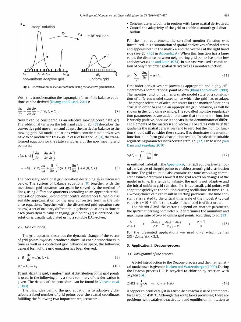
The implementation of the adaptive grid is carried out througha coordinate transformation depicted in Fig. 1. The physical (real)solution u(x, t), including ‘steep’ fronts, is now considered along anon-uniform adaptive coordinate x(t). Through the transformation,this solution is mapped to a computational uniform coordinate sys-tem (�, �). Here the solution �(�, �) becomes ‘milder’. The balanceequations are now considered along this computational coordinateand are therefore easier to solve. To be more precise, the regulartransformation (5)–(6) maps the ‘steep’ solution of the state u(x, t)

: (x, t) → (�, �) (5)

t(�, �) = � (6)

R. Kelling et al. / Computers and Chemica

x0 xi xnxi+1xi-1

u

x

‘steep‘ solution

non-uniform adaptive grid

ννΦΦ

ξξ

‘mild‘ solution

uniform gridΔξΔξ

t

Wt

NTcmhfp

a

Tbmlcsabes

2

otg

x

Tig(

tf

2

Fig. 1. Discretization in spatial coordinate using the adaptive grid method.

ith this transformation the Lagrangian form of the balance equa-ions can be derived (Huang and Russel, 2011):

∂u

∂t− ∂u

∂x

∂x

∂t= f (u, t, x(t)) . (7)

ow x can be considered as an adaptive moving coordinate x(t).he additional term on the left hand side of Eq. (7) describes theonvective grid movement and adapts the particular balance to theoving grid. All model equations which contain time derivatives

ave to be modified in this way. In case of balance Eq. (3), the trans-ormed equation for the state variables u at the now moving gridoints is:

(u, t, x)

(∂u

∂t− ∂u

∂x

∂x

∂t

)

= −b (u, t, x)∂u

∂x+ ∂

∂x

(c (u, t, x)

∂u

∂x

)+ d (u, t, x) . (8)

he necessary additional grid equation describing ∂x∂t

is discussedelow. The system of balance equations (8) together with theentioned grid equation can again be solved by the method of

ines, using difference quotients according to an appropriate dis-retization scheme. Second order central differences turned out asuitable approximation for the new convective term in the bal-nce equations. Together with the discretized grid equation (seeelow) a set of ordinary differential-algebraic equations in time atach (now dynamically changing) grid point xi(t) is obtained. Theolution is usually calculated using a suitable DAE-solver.

.3. Grid equation

The grid equation describes the dynamic change of the vectorf grid points ∂x/∂t as introduced above. To enable smoothness inime as well as a controlled grid behavior in space, the followingeneral form of the grid equation has been derived:

Bdx

dt= s(u, t, x), (9)

(t = 0) = x0. (10)

o initialize the grid, a uniform initial distribution of the grid pointss used. In the following only a short summary of the derivation isiven. The details of the procedure can be found in Verwer et al.

1988).

The basic idea behind the grid equation is to adaptively dis-ribute a fixed number of grid points over the spatial coordinate,ulfilling the following two important requirements:

l Engineering 71 (2014) 467–477 469

• Concentrate grid points in regions with large spatial derivatives.• Control the adaptivity of the grid to enable a smooth grid distri-

bution.

For the first requirement, the so-called monitor function ω isintroduced. It is a summation of spatial derivatives of model statesand appears both in the matrix B and the vector s of the right handside (see Eq. (40) in Appendix A). When this function has a largevalue, the distance between neighboring grid points has to be lowand vice versa (de and Boor, 1974). In our case we used a combina-tion of only first order spatial derivatives as monitor function:

ω =∑

s

∣∣∣∣∂us

∂x

∣∣∣∣ + ˛s(t). (11)

First order derivatives are proven as appropriate and highly effi-cient from a computational point of view (Blom and Verwer, 1989).The monitor function defines a single model state or a combina-tion of different model states us, to which the grid has to adapt.The proper selection of adequate states for the monitor function iscrucial in order to enable an appropriate grid behavior, as will beshown in the following example. The so-called monitor regulariza-tion parameters ˛s are added to ensure that the monitor functionis strictly positive, because it appears in the denominator of differ-ent elements of the matrix B and vector s. For states with very flatgradients the spatial derivatives tend to zero, but the monitor func-tion should still consider these states. If ˛s dominates the monitorfunction, a uniform grid distribution results. To calculate suitableregularizing parameters for a certain state, Eq. (12) can be used (vanDam and Zegeling, 2010):

˛s(t) =∫ L

0

∣∣∣∣∂us

∂x

∣∣∣∣dx. (12)

As outlined in detail in the Appendix A, matrix B couples five tempo-ral derivatives of the grid points to enable a smooth grid distributionin time. The grid equation also contains the time smoothing param-eter which determines how fast the grid reacts on changes of themodel in time. If tends to infinity, the grid is not adaptive andthe initial uniform grid remains. If is too small, grid points willadapt too quickly to the solution causing oscillations in time. Thus,a wrong choice of can result in starting problems. The time con-stant is related to the critical time scale of the model. A typicalvalue is = 10−3, if the time scale of the model is of first order.

The Matrix B and the vector s depend on another parameter,the spatial smoothing parameter �. It determines the minimum andmaximum ratio of two adjoining grid points according to Eq. (13).

�

� + 1<

�xi+1

�xi= xi+2 − xi+1

xi+1 − xi<

� + 1�

(13)

For the presented applications we used � = 2 which defines2/3 < �xi+1/�xi < 3/2.

3. Application I: Deacon-process

3.1. Background of the process

A brief introduction to the Deacon-process and the mathemati-cal model used is given in Nieken and Watzenberger (1999). Duringthe Deacon-process HCl is recycled to chlorine by reaction withoxygen (14).

2 HCl + 1O2 � Cl2 + H2O (14)

A copper chloride catalyst in a fixed-bed reactor is used at tempera-tures around 450 ◦C. Although this route looks promising, there areproblems with catalyst deactivation and equilibrium limitation to

4 emica

lthasds

2

C

fsN

3

ted

�

�

(

(

(

0

T(tpncdtRA

bs

70 R. Kelling et al. / Computers and Ch

ess than 84% at 350 ◦C, causing unwanted byproducts which haveo be separated from the product stream. Thus, two-stage processesave been proposed (Deacon, 1875; Agar et al., 1997). Here, the cat-lyst fixed bed is used as chlorine storage during the chlorinationtage (15). By means of oxygen the chlorine is removed during theechloration stage (16), the copper is oxidized and the cycle cantart again.

HCl + CuO → CuCl2 + H2O (15)

uCl2 + 12

O2 → CuO + Cl2 (16)

Equilibrium limitations are avoided by this storage effect. In theollowing, the adaptive grid method is applied to the chlorinationtage only. For this purpose the mathematical model suggested inieken and Watzenberger (1999) has been adopted.

.2. Model for chlorination stage

A quasi-homogeneous one-dimensional model of a tubular reac-or is used. It is assumed that there is no loss of copper. The balancequations (17)–(22) with corresponding Dankwerts boundary con-itions and initial conditions are considered.

G ∂wHCl

∂t= − m

A

∂wHCl

∂x+ D

∂2wHCl

∂x2− wHCl

1A

∂m

∂x− 2MWHCl r

(17)

G ∂wH2O

∂t= − m

A

∂wH2O

∂x+ D

∂2wH2O

∂x2− wH2O

1A

∂m

∂x+ MWH2O r

(18)

1 − �)ScSp

∂T

∂t= − m

AcG

p∂T

∂x+ �

∂2T

∂x2− cG

p T1A

∂m

∂x− �hr r (19)

1 − �)∂cCuCl2

∂t= r (20)

1 − �)∂cCuO

∂t= −r (21)

= − 1A

∂m

∂x+ r (MWCuO − MWCuCl2 ) (22)

hey contain the component mass balances for the gaseous specieshydrogen chloride wHCl and water wH2O) and the enthalpy balanceo calculate the temperature with accumulation, convection, dis-ersion, and reaction source terms. Convection and dispersion areeglected in the mass balances of the immobilized solids (copperhloride cCuCl2 and copper oxide cCuO). The mass flow is changingue to storage and release of chlorine in the solid phase. To describehis effect the quasi stationary total mass balance (22) is used.eaction rates and model parameters are listed in the Appendix.

The first order spatial derivatives are discretized with first-orderackward differences (23) and the second order derivatives withecond-order central differences (24).

∂u

∂x

∣∣∣∣i

≈ ui − ui−1

xi − xi−1(23)

∂2u

∂x2

∣∣∣∣ ≈ 2 ui−1

(x − x ) (x − x )+ 2 ui

(x − x ) (x − x )

i i−1 i i−1 i+1 i i−1 i i+1

+ 2 ui+1

(xi+1 − xi−1) (xi+1 − xi)(24)

l Engineering 71 (2014) 467–477

The model is implemented in ProMoT (Mirschel et al., 2009)enabling the simulation with the IDA-solver from SUNDIALS(Hindmarsh et al., 2005), using the dynamic simulation and numer-ical analysis tool DIANA (Krasnyk et al., 2006). The approximationin time is carried out with variable-order, variable-coefficient back-ward differences. The solution of the resulting nonlinear system isaccomplished with a modified Newton iteration.

3.3. Results with an equidistant grid

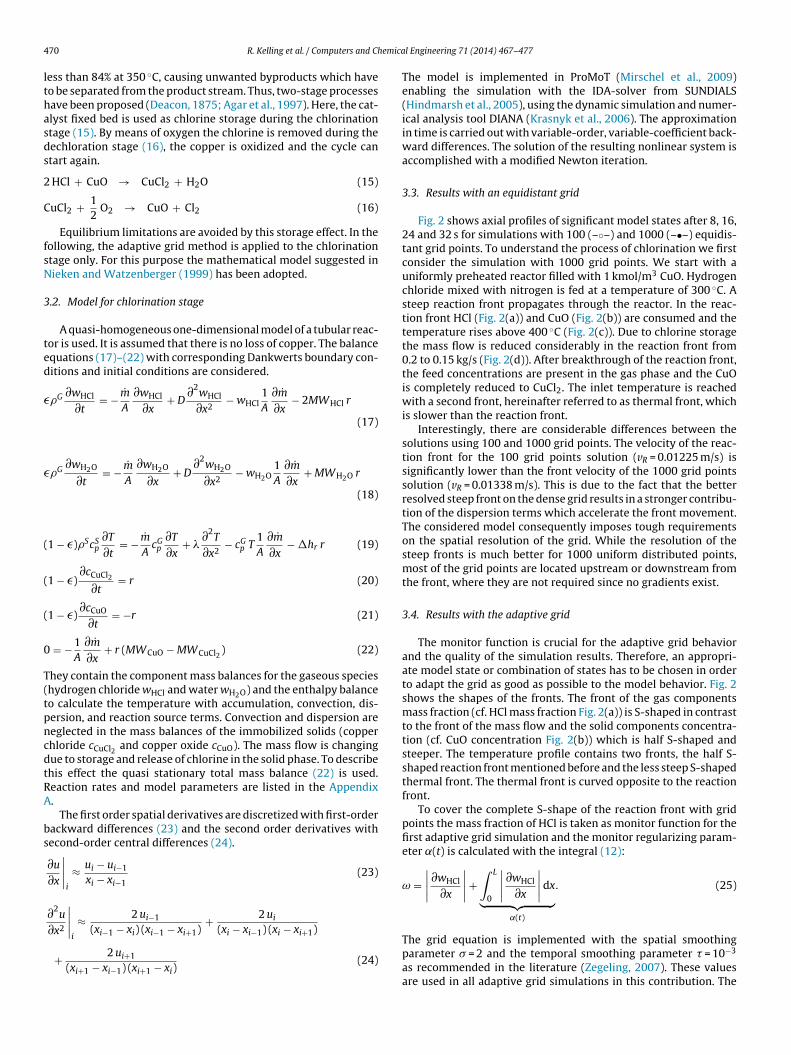
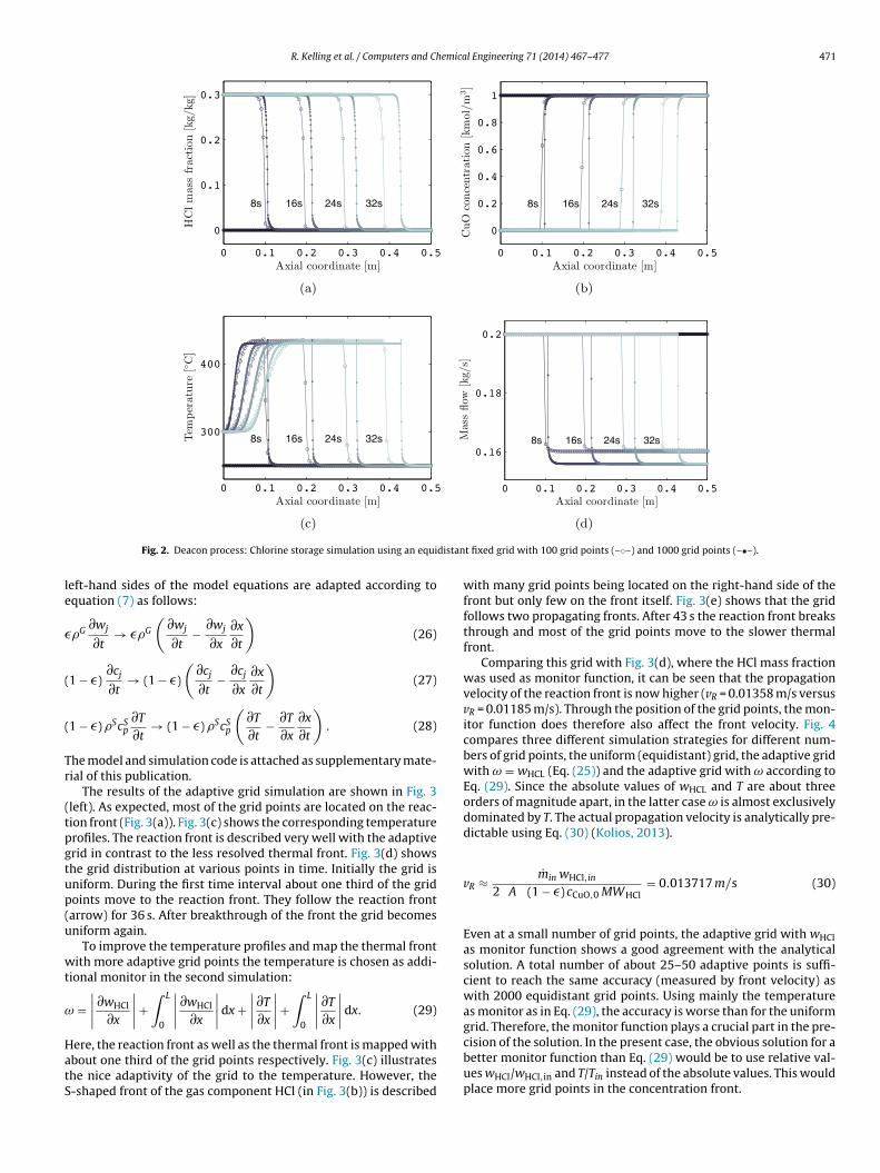
Fig. 2 shows axial profiles of significant model states after 8, 16,24 and 32 s for simulations with 100 (–◦–) and 1000 (–•–) equidis-tant grid points. To understand the process of chlorination we firstconsider the simulation with 1000 grid points. We start with auniformly preheated reactor filled with 1 kmol/m3 CuO. Hydrogenchloride mixed with nitrogen is fed at a temperature of 300 ◦C. Asteep reaction front propagates through the reactor. In the reac-tion front HCl (Fig. 2(a)) and CuO (Fig. 2(b)) are consumed and thetemperature rises above 400 ◦C (Fig. 2(c)). Due to chlorine storagethe mass flow is reduced considerably in the reaction front from0.2 to 0.15 kg/s (Fig. 2(d)). After breakthrough of the reaction front,the feed concentrations are present in the gas phase and the CuOis completely reduced to CuCl2. The inlet temperature is reachedwith a second front, hereinafter referred to as thermal front, whichis slower than the reaction front.

Interestingly, there are considerable differences between thesolutions using 100 and 1000 grid points. The velocity of the reac-tion front for the 100 grid points solution (vR = 0.01225 m/s) issignificantly lower than the front velocity of the 1000 grid pointssolution (vR = 0.01338 m/s). This is due to the fact that the betterresolved steep front on the dense grid results in a stronger contribu-tion of the dispersion terms which accelerate the front movement.The considered model consequently imposes tough requirementson the spatial resolution of the grid. While the resolution of thesteep fronts is much better for 1000 uniform distributed points,most of the grid points are located upstream or downstream fromthe front, where they are not required since no gradients exist.

3.4. Results with the adaptive grid

The monitor function is crucial for the adaptive grid behaviorand the quality of the simulation results. Therefore, an appropri-ate model state or combination of states has to be chosen in orderto adapt the grid as good as possible to the model behavior. Fig. 2shows the shapes of the fronts. The front of the gas componentsmass fraction (cf. HCl mass fraction Fig. 2(a)) is S-shaped in contrastto the front of the mass flow and the solid components concentra-tion (cf. CuO concentration Fig. 2(b)) which is half S-shaped andsteeper. The temperature profile contains two fronts, the half S-shaped reaction front mentioned before and the less steep S-shapedthermal front. The thermal front is curved opposite to the reactionfront.

To cover the complete S-shape of the reaction front with gridpoints the mass fraction of HCl is taken as monitor function for thefirst adaptive grid simulation and the monitor regularizing param-eter ˛(t) is calculated with the integral (12):

ω =∣∣∣∣∂wHCl

∂x

∣∣∣∣ +∫ L

0

∣∣∣∣∂wHCl

∂x

∣∣∣∣dx

︸ ︷︷ ︸˛(t)

. (25)

The grid equation is implemented with the spatial smoothingparameter � = 2 and the temporal smoothing parameter = 10−3

as recommended in the literature (Zegeling, 2007). These valuesare used in all adaptive grid simulations in this contribution. The

R. Kelling et al. / Computers and Chemical Engineering 71 (2014) 467–477 471

distan

le

�

(

(

Tr

(tpgtup(u

wt

ω

HatS

Fig. 2. Deacon process: Chlorine storage simulation using an equi

eft-hand sides of the model equations are adapted according toquation (7) as follows:

G ∂wj

∂t→ �G

(∂wj

∂t− ∂wj

∂x

∂x

∂t

)(26)

1 − �)∂cj

∂t→ (1 − �)

(∂cj

∂t− ∂cj

∂x

∂x

∂t

)(27)

1 − �) ScSp

∂T

∂t→ (1 − �) ScS

p

(∂T

∂t− ∂T

∂x

∂x

∂t

). (28)

he model and simulation code is attached as supplementary mate-ial of this publication.

The results of the adaptive grid simulation are shown in Fig. 3left). As expected, most of the grid points are located on the reac-ion front (Fig. 3(a)). Fig. 3(c) shows the corresponding temperaturerofiles. The reaction front is described very well with the adaptiverid in contrast to the less resolved thermal front. Fig. 3(d) showshe grid distribution at various points in time. Initially the grid isniform. During the first time interval about one third of the gridoints move to the reaction front. They follow the reaction frontarrow) for 36 s. After breakthrough of the front the grid becomesniform again.

To improve the temperature profiles and map the thermal frontith more adaptive grid points the temperature is chosen as addi-

ional monitor in the second simulation:

=∣∣∣∣∂wHCl

∂x

∣∣∣∣ +∫ L

0

∣∣∣∣∂wHCl

∂x

∣∣∣∣dx +∣∣∣∣∂T

∂x

∣∣∣∣ +∫ L

0

∣∣∣∣∂T

∂x

∣∣∣∣dx. (29)

ere, the reaction front as well as the thermal front is mapped withbout one third of the grid points respectively. Fig. 3(c) illustrateshe nice adaptivity of the grid to the temperature. However, the-shaped front of the gas component HCl (in Fig. 3(b)) is described

t fixed grid with 100 grid points (–◦–) and 1000 grid points (–•–).

with many grid points being located on the right-hand side of thefront but only few on the front itself. Fig. 3(e) shows that the gridfollows two propagating fronts. After 43 s the reaction front breaksthrough and most of the grid points move to the slower thermalfront.

Comparing this grid with Fig. 3(d), where the HCl mass fractionwas used as monitor function, it can be seen that the propagationvelocity of the reaction front is now higher (vR = 0.01358 m/s versusvR = 0.01185 m/s). Through the position of the grid points, the mon-itor function does therefore also affect the front velocity. Fig. 4compares three different simulation strategies for different num-bers of grid points, the uniform (equidistant) grid, the adaptive gridwith ω = wHCL (Eq. (25)) and the adaptive grid with ω according toEq. (29). Since the absolute values of wHCL and T are about threeorders of magnitude apart, in the latter case ω is almost exclusivelydominated by T. The actual propagation velocity is analytically pre-dictable using Eq. (30) (Kolios, 2013).

vR ≈ min wHCl,in

2 A (1 − �) cCuO,0 MWHCl= 0.013717 m/s (30)

Even at a small number of grid points, the adaptive grid with wHClas monitor function shows a good agreement with the analyticalsolution. A total number of about 25–50 adaptive points is suffi-cient to reach the same accuracy (measured by front velocity) aswith 2000 equidistant grid points. Using mainly the temperatureas monitor as in Eq. (29), the accuracy is worse than for the uniformgrid. Therefore, the monitor function plays a crucial part in the pre-

cision of the solution. In the present case, the obvious solution for abetter monitor function than Eq. (29) would be to use relative val-ues wHCl/wHCl,in and T/Tin instead of the absolute values. This wouldplace more grid points in the concentration front.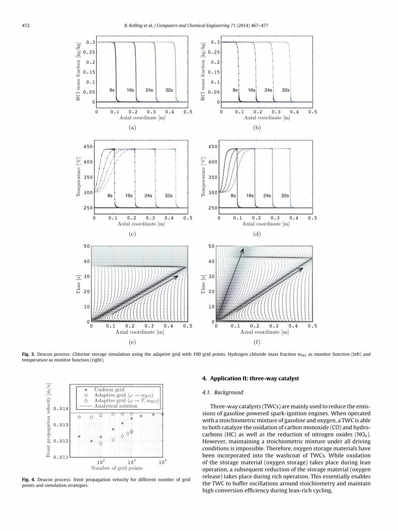

472 R. Kelling et al. / Computers and Chemical Engineering 71 (2014) 467–477

Fig. 3. Deacon process: Chlorine storage simulation using the adaptive grid with 100

temperature as monitor function (right).

Fig. 4. Deacon process: front propagation velocity for different number of gridpoints and simulation strategies.

grid points. Hydrogen chloride mass fraction wHCl as monitor function (left) and

4. Application II: three-way catalyst

4.1. Background

Three-way catalysts (TWCs) are mainly used to reduce the emis-sions of gasoline powered spark-ignition engines. When operatedwith a stoichiometric mixture of gasoline and oxygen, a TWC is ableto both catalyze the oxidation of carbon monoxide (CO) and hydro-carbons (HC) as well as the reduction of nitrogen oxides (NOx).However, maintaining a stoichiometric mixture under all drivingconditions is impossible. Therefore, oxygen storage materials havebeen incorporated into the washcoat of TWCs. While oxidationof the storage material (oxygen storage) takes place during lean

operation, a subsequent reduction of the storage material (oxygenrelease) takes place during rich operation. This essentially enablesthe TWC to buffer oscillations around stoichiometry and maintainhigh conversion efficiency during lean-rich cycling.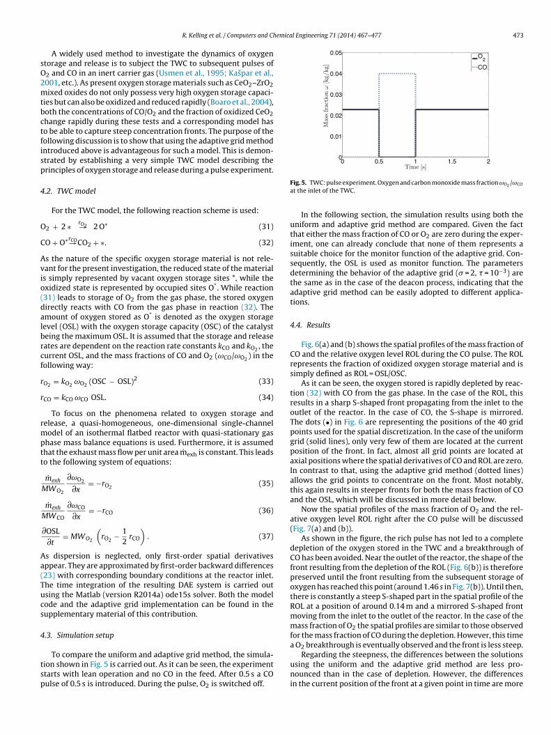

emical Engineering 71 (2014) 467–477 473

sO2mtbctfisp

4

O

C

Avio(dalbrcf

r

r

rmptt

Aa(Tucs

4

tsp

R. Kelling et al. / Computers and Ch

A widely used method to investigate the dynamics of oxygentorage and release is to subject the TWC to subsequent pulses of2 and CO in an inert carrier gas (Usmen et al., 1995; Kaspar et al.,001, etc.). As present oxygen storage materials such as CeO2–ZrO2ixed oxides do not only possess very high oxygen storage capaci-

ies but can also be oxidized and reduced rapidly (Boaro et al., 2004),oth the concentrations of CO/O2 and the fraction of oxidized CeO2hange rapidly during these tests and a corresponding model haso be able to capture steep concentration fronts. The purpose of theollowing discussion is to show that using the adaptive grid methodntroduced above is advantageous for such a model. This is demon-trated by establishing a very simple TWC model describing therinciples of oxygen storage and release during a pulse experiment.

.2. TWC model

For the TWC model, the following reaction scheme is used:

2 + 2 ∗ rO2→ 2 O∗ (31)

O + O∗rCO→CO2 + ∗. (32)

s the nature of the specific oxygen storage material is not rele-ant for the present investigation, the reduced state of the materials simply represented by vacant oxygen storage sites *, while thexidized state is represented by occupied sites O*. While reaction31) leads to storage of O2 from the gas phase, the stored oxygenirectly reacts with CO from the gas phase in reaction (32). Themount of oxygen stored as O* is denoted as the oxygen storageevel (OSL) with the oxygen storage capacity (OSC) of the catalysteing the maximum OSL. It is assumed that the storage and releaseates are dependent on the reaction rate constants kCO and kO2 , theurrent OSL, and the mass fractions of CO and O2 (ωCO/ωO2 ) in theollowing way:

O2 = kO2 ωO2 (OSC − OSL)2 (33)

CO = kCO ωCO OSL. (34)

To focus on the phenomena related to oxygen storage andelease, a quasi-homogeneous, one-dimensional single-channelodel of an isothermal flatbed reactor with quasi-stationary gas

hase mass balance equations is used. Furthermore, it is assumedhat the exhaust mass flow per unit area mexh is constant. This leadso the following system of equations:

mexh

MWO2

∂ωO2

∂x= −rO2 (35)

mexh

MWCO

∂ωCO

∂x= −rCO (36)

∂OSL∂t

= MWO2

(rO2 − 1

2rCO

). (37)

s dispersion is neglected, only first-order spatial derivativesppear. They are approximated by first-order backward differences23) with corresponding boundary conditions at the reactor inlet.he time integration of the resulting DAE system is carried outsing the Matlab (version R2014a) ode15s solver. Both the modelode and the adaptive grid implementation can be found in theupplementary material of this contribution.

.3. Simulation setup

To compare the uniform and adaptive grid method, the simula-ion shown in Fig. 5 is carried out. As it can be seen, the experimenttarts with lean operation and no CO in the feed. After 0.5 s a COulse of 0.5 s is introduced. During the pulse, O2 is switched off.

Fig. 5. TWC: pulse experiment. Oxygen and carbon monoxide mass fraction ωO2 /ωCO

at the inlet of the TWC.

In the following section, the simulation results using both theuniform and adaptive grid method are compared. Given the factthat either the mass fraction of CO or O2 are zero during the exper-iment, one can already conclude that none of them represents asuitable choice for the monitor function of the adaptive grid. Con-sequently, the OSL is used as monitor function. The parametersdetermining the behavior of the adaptive grid (� = 2, = 10−3) arethe same as in the case of the deacon process, indicating that theadaptive grid method can be easily adopted to different applica-tions.

4.4. Results

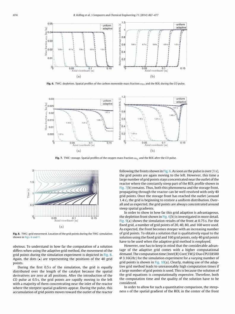
Fig. 6(a) and (b) shows the spatial profiles of the mass fraction ofCO and the relative oxygen level ROL during the CO pulse. The ROLrepresents the fraction of oxidized oxygen storage material and issimply defined as ROL = OSL/OSC.

As it can be seen, the oxygen stored is rapidly depleted by reac-tion (32) with CO from the gas phase. In the case of the ROL, thisresults in a sharp S-shaped front propagating from the inlet to theoutlet of the reactor. In the case of CO, the S-shape is mirrored.The dots (•) in Fig. 6 are representing the positions of the 40 gridpoints used for the spatial discretization. In the case of the uniformgrid (solid lines), only very few of them are located at the currentposition of the front. In fact, almost all grid points are located ataxial positions where the spatial derivatives of CO and ROL are zero.In contrast to that, using the adaptive grid method (dotted lines)allows the grid points to concentrate on the front. Most notably,this again results in steeper fronts for both the mass fraction of COand the OSL, which will be discussed in more detail below.

Now the spatial profiles of the mass fraction of O2 and the rel-ative oxygen level ROL right after the CO pulse will be discussed(Fig. 7(a) and (b)).

As shown in the figure, the rich pulse has not led to a completedepletion of the oxygen stored in the TWC and a breakthrough ofCO has been avoided. Near the outlet of the reactor, the shape of thefront resulting from the depletion of the ROL (Fig. 6(b)) is thereforepreserved until the front resulting from the subsequent storage ofoxygen has reached this point (around 1.46 s in Fig. 7(b)). Until then,there is constantly a steep S-shaped part in the spatial profile of theROL at a position of around 0.14 m and a mirrored S-shaped frontmoving from the inlet to the outlet of the reactor. In the case of themass fraction of O2 the spatial profiles are similar to those observedfor the mass fraction of CO during the depletion. However, this timea O2 breakthrough is eventually observed and the front is less steep.

Regarding the steepness, the differences between the solutionsusing the uniform and the adaptive grid method are less pro-nounced than in the case of depletion. However, the differencesin the current position of the front at a given point in time are more

474 R. Kelling et al. / Computers and Chemical Engineering 71 (2014) 467–477

Fig. 6. TWC: depletion. Spatial profiles of the carbon monoxide mass fraction ωCO and the ROL during the CO pulse.

Fig. 7. TWC: storage. Spatial profiles of the oxygen m

Fs

odgAp

ddCwwa

ig. 8. TWC: grid movement. Location of the grid points during the TWC-simulationhown in Figs. 6 and 7.

bvious. To understand in how far the computation of a solutioniffers when using the adaptive grid method, the movement of therid points during the simulation experiment is depicted in Fig. 8.gain, the dots (•) are representing the positions of the 40 gridoints.

During the first 0.5 s of the simulation, the grid is equallyistributed over the length of the catalyst because the spatialerivatives are zero at all positions. After the introduction of the

O pulse at 0.5 s, the grid points are rapidly moving to the leftith a majority of them concentrating near the inlet of the reactorhere the steepest spatial gradients appear. During the pulse, this

ccumulation of grid points moves toward the outlet of the reactor

ass fraction ωO2 and the ROL after the CO pulse.

following the fronts shown in Fig. 6. As soon as the pulse is over (1 s),the grid points are again moving to the left. However, this time alarge number of grid points stays concentrated near the outlet of thereactor where the constantly steep part of the ROL profile shown inFig. 7(b) remains. Thus, both this phenomena and the storage front,propagating through the reactor can be well resolved with only 40grid points. Once the storage front has reached the outlet (around1.4 s), the grid is beginning to restore a uniform distribution. Over-all and as expected, the grid points are always concentrated aroundsteep spatial gradients.

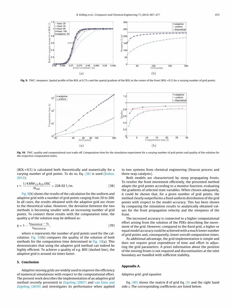
In order to show in how far this grid adaption is advantageous,the depletion front shown in Fig. 6(b) is investigated in more detail.Fig. 9(a) shows the simulation results of the front at 0.75 s. For thefixed grid, a number of grid points of 20, 40, 80, and 160 were used.As expected, the front becomes steeper with an increasing numberof grid points. To obtain a solution that is qualitatively equal to thesolution using the fixed grid and 160 grid points, only 40 grid pointshave to be used when the adaptive grid method is employed.

However, one has to keep in mind that the considerable advan-tage of the adaptive grid comes with a higher computationaldemand. The computation time (Intel(R) Core(TM)2 Duo CPU E8500@ 3.16GHz) for the simulation experiment for a varying number ofgrid points is shown in Fig. 10(a). Clearly, making use of the adap-tive grid method leads to unreasonably high computation times ifa large number of grid points is used. This is because the solution ofthe grid equations is computationally expensive. Therefore, both

the computation time and the quality of the solution have to beconsidered.

In order to allow for such a quantitative comparison, the steep-ness s of the spatial gradient of the ROL in the center of the front

R. Kelling et al. / Computers and Chemical Engineering 71 (2014) 467–477 475

Fig. 9. TWC: steepness. Spatial profile of the ROL at 0.75 s and the spatial gradient of the ROL in the center of the front (ROL = 0.5) for a varying number of grid points.

F imulat

(v2

s

aItmpq

q

cmdha

5

oTmZ

ig. 10. TWC: quality and computational cost trade-off. Computation time for the she respective computation times.

ROL = 0.5) is calculated both theoretically and numerically for aarying number of grid points. To do so, Eq. (38) is used (Kolios,013):

≈ 1/4 MWCO kCO OSCmexh

= 228.02 1/m. (38)

Fig. 9(b) shows the results of the calculation for the uniform anddaptive grid with a number of grid points ranging from 20 to 200.n all cases, the results obtained with the adaptive grid are closero the theoretical value. However, the deviation between the two

ethods is becoming smaller with an increasing number of gridoints. To connect these results with the computation time, theuality q of the solution may be defined as:

= 1 − stheoretical − sn

stheoretical, (39)

where n represents the number of grid points used for the cal-ulation. Fig. 10(b) compares the quality of the solution of bothethods for the computation time determined in Fig. 10(a). This

emonstrates that using the adaptive grid method can indeed beighly efficient. To achieve a quality of e.g. 80% (dashed line), thedaptive grid is around six times faster.

. Conclusion

Adaptive moving grids are widely used to improve the efficiency

f numerical simulations with respect to the computational effort.he present work describes the implementation of an adaptive gridethod recently presented in Zegeling (2007) and van Dam and

egeling (2010) and investigates its performance when applied

tion experiment for a varying number of grid points and quality of the solution for

to two systems from chemical engineering (Deacon process andthree-way catalysts).

Both models are characterized by steep propagating fronts.To resolve the front movement efficiently, the presented methodadapts the grid points according to a monitor function, evaluatingthe gradients of selected state variables. When chosen adequately,it could be shown that, for a given number of grid points, themethod clearly outperforms a fixed uniform distribution of the gridpoints with respect to the model accuracy. This has been shownby comparing the simulation results to analytically obtained val-ues for the front propagation velocity and the steepness of thefront.

The increased accuracy is connected to a higher computationaleffort arising from the solution of the PDEs describing the move-ment of the grid. However, compared to the fixed grid, a higher orequal model accuracy could be achieved with a much lower numberof grid points and, consequently, lower overall computation times.

As additional advantage, the grid implementation is simple anddoes not require great expenditure of time and effort in adjus-ting the grid parameters. A priori information about the positionof the moving fronts is not required and discontinuities at the inletboundary are handled with sufficient stability.

Appendix A.

Adaptive grid: grid equation

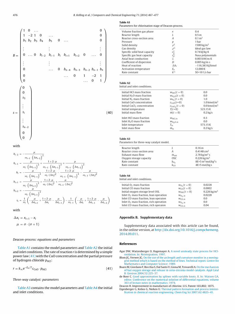
Eq. (40) shows the matrix B of grid Eq. (9) and the right handside s. The corresponding coefficients are listed below.

4 emical Engineering 71 (2014) 467–477

B

s

w

w

D

apo

r

T

a

Table A1Parameters for chlorination stage of Deacon-process.

Volume fraction gas phase � 0.4Reactor length L 0.5 mReactor cross-section area A 0.1 m2

Pressure p 1 barSolid density S 1500 kg/m3

Gas density G Ideal gas lawSpecific solid heat capacity cS

p 0.74 kJ/kg KSpecific gas heat capacity cG

p Nasa polynomialsAxial heat conduction � 0.003 kW/m KCoefficient of dispersion D 0.005 kg/m sHeat of reaction �hr −116,383 kJ/kmolActivation temperature Ea 12,000 KRate constant k∞ 5E+10 1/s bar

Table A2Initial and inlet conditions.

Initial HCl mass fraction wHCl(t = 0) 0.0Initial H2O mass fraction wH2O(t = 0) 0.0Initial N2 mass fraction wN2 (t = 0) 1.0Initial CuO concentration cCuO(t = 0) 1.0 kmol/m3

Initial CuCl2 concentration cCuCl2 (t = 0) 0.0 kmol/m3

Initial temperature T(t = 0) 523.15 KInitial mass flow m(t = 0) 0.2 kg/s

Inlet HCl mass fraction wHCl,in 0.3Inlet H2O mass fraction wH2O,in 0.0Inlet temperature Tin 573.15 KInlet mass flow min 0.2 kg/s

Table A3Parameters for three-way catalyst model.

Reactor length L 0.16 mReactor cross-section area A 0.4148 cm2

Exhaust mass flow mexh 2.78 kg/m2 sOxygen storage capacity OSC 0.226 kg/m3

Rate constant kO2 8E+5 m3mol/kg2sRate constant kCO 4E+5 mol/kg s

Table A4Initial and inlet conditions.

Initial O2 mass fraction wO2 (t = 0) 0.0228Initial CO mass fraction wCO(t = 0) 0.0002Initial oxygen storage level OSL wOSL(t = 0) 0.226 kg/m3

Inlet O2 mass fraction, lean operation wO2,in 0.0228Inlet CO mass fraction, lean operaion wCO,in 0.0

76 R. Kelling et al. / Computers and Ch

=

⎛⎜⎜⎜⎜⎜⎜⎜⎜⎜⎜⎜⎜⎜⎜⎜⎜⎜⎝

1 0 . . . 0

1 −2 1 0 . . . 0

b1 b2 b3 b4 b5 0 . . . 0

......

...

0 . . . 0 bi−2 bi−1 bi bi+1 bi+2 0 . . . 0

......

...

0 . . . 0 bn−4 bn−3 bn−2 bn−1 bn

0 . . . 0 1 −2 1

0 . . . 0 1

⎞⎟⎟⎟⎟⎟⎟⎟⎟⎟⎟⎟⎟⎟⎟⎟⎟⎟⎠

=

⎛⎜⎜⎜⎜⎜⎜⎜⎜⎜⎜⎜⎜⎜⎜⎜⎜⎜⎝

0

0

s3

...

si

...

sn−2

0

0

⎞⎟⎟⎟⎟⎟⎟⎟⎟⎟⎟⎟⎟⎟⎟⎟⎟⎟⎠

(40)

ith

bi−2 = − �

ωi−1 ·(

�xi−2

)2

bi−1 = �

ωi ·(

�xi−1

)2+ 1 + 2 · �

ωi−1 ·(

�xi−1

)2+ �

ωi−1 ·(

�xi−2

)2

bi = − �

ωi ·(

�xi−1

)2− 1 + 2 · �

ωi · (�xi)2

− 1 + 2 · �

ωi−1 ·(

�xi−1

)2− �

ωi−1 · (�xi)2

bi+1 = �

ωi ·(

�xi+1

)2+ 1 + 2 · �

ωi · (�xi)2

+ �

ωi−1 · (�xi)2

bi+2 = − �

ωi ·(

�xi+1

)2

si = 1ωi

(− �

�xi+1+ 1 + 2 · �

�xi− �

�xi−1

)− 1

ωi−1

(− �

�xi+ 1 + 2 · �

�xi−1− �

�xi−2

)

ith

�xi = xi+1 − xi

� = � · (� + 1)

eacon-process: equations and parameters

Table A1 contains the model parameters and Table A2 the initialnd inlet conditions. The rate of reaction r is determined by a simpleower law (41) with the CuO concentration and the partial pressuref hydrogen chloride pHCl:

= k∞e−Ea/T cCuO · pHCl (41)

hree-way catalyst: parameters

Table A3 contains the model parameters and Table A4 the initialnd inlet conditions.

Inlet O2 mass fraction, rich operation wO2,in 0.0Inlet CO mass fraction, rich operaion wCO,in 0.04

Appendix B. Supplementary data

Supplementary data associated with this article can be found,in the online version, at http://dx.doi.org/10.1016/j.compchemeng.2014.09.011.

References

Agar DW, Watzenberger O, Hagemayer A. A novel unsteady state process for HCl-oxidation. In: Reintegration; 1997.

Blom JG, Verwer JG. On the use of the arclength and curvature monitor in a moving-grid method which is based on the method of lines. Technical report. Centre forMathematics and Computer Science; 1989.

Boaro M, Giordano F, Recchia S, Dal Santo V, Giona M, Trovarelli A. On the mechanismof fast oxygen storage and release in ceria-zirconia model catalysts. Appl CatalB: Environ 2004;52:225–37.

de Boor C. Good approximation by splines with variable knots. II. In: Watson GA,editor. Conference on the numerical solution of differential equations, volume

363 of lecture notes in mathematics; 1974.

Deacon H. Improvement in manufacture of chlorine. U.S. Patent 165,802; 1875.Eigenberger G, Kolios G, Nieken U. Thermal pattern formation and process intensi-

fication in chemical reaction engineering. Chem Eng Sci 2007;62:4825–41.

emica

H

HK

K

K

M

R. Kelling et al. / Computers and Ch

indmarsh AC, Brown PN, Grant KE, Lee SL, Serban R, Shumaker DE,et al. Sundials: suite of nonlinear and differential/algebraic equa-tion solvers. ACM Trans Math Softw 2005;31(September (3)):363–96,http://dx.doi.org/10.1145/1089014.1089020, ISSN 0098-3500.

uang W, Russel RD. Adaptive moving mesh methods. New York: Springer; 2011.aspar J, Di Monte R, Fornasiero P, Graziani M, Bradshaw H, Norman C. Dependency

of the oxygen storage capacity in zirconia-ceria solid solutions upon texturalproperties. Top Catal 2001;16/17:83–7.

olios G. (Habilitation thesis) Regenerative fixed-bed processes: approximativeanalysis and efficient computation of the cyclic steady state (Habilitation thesis).University of Stuttgart; 2013.

rasnyk M, Bondareva K, Milokhov O, Teplinskiy K, Ginkel M, Kienle A. The pro-mot/diana simulation environment. In: Marquardt W, Pantelides C, editors. 16thEuropean symposium on computer aided process engineering and 9th inter-national symposium on process systems engineering, volume 21 of Computer

aided chemical engineering. Elsevier; 2006. p. 445–50, DOI: 10.1016/S1570-7946(06)80086-6.

irschel S, Steinmetz K, Rempel M, Ginkel M, Gilles ED. Promot: mod-ular modeling for systems biology. Bioinformatics 2009;25(5):687–9,http://dx.doi.org/10.1093/bioinformatics/btp029.

l Engineering 71 (2014) 467–477 477

Nieken U, Watzenberger O. Periodic operation of the deacon process. Chem Eng Sci1999;54(13-14):2619–26, http://dx.doi.org/10.1016/S0009-2509(98)00490-4,ISSN 0009-2509.

Nowak U, Frauhammer J, Nieken U. A fully adaptive algorithm for parabolicpartial differential equations in one space dimension. Comput Chem Eng1996;20:547–61.

Usmen RK, Graham GW, Watkins WLH, McCabe RW. Incorporation of La3+ into aPt/CeO2/Al2O3 catalyst. Catal Lett 1995;30:53–63.

van Dam A, Zegeling PA. Balanced monitoring of flow phenomena in moving meshmethods. Commun Comput Phys 2010;7:138–70.

Verwer JG, Blom JG, Furzeland RM, Zegeling PA. A moving-grid method forone-dimensional PDEs based on the method of lines. Technical report. Depart-ment of Numerical Mathematics, Centrum voor Wiskunde en Informatica;1988.

Zegeling PA. Theory and application of adaptive moving grid methods. In: Tang T,

Xu J, editors. Adaptive computations: theory and algorithms; 2007.

Zegeling PA, Kok HP. Adaptive moving mesh computations for reaction–diffusionsystems. J Comput Appl Math 2004;168:519–28.

Zegeling PA, de Boer W, Tang H. Robust and efficient adaptive moving mesh solutionof the 2-D Euler equations. Contemp Math 2005;383:419–30.