Computer Animation3-Interpolation

SS 13

Prof. Dr. Charles A. Wüthrich,Fakultät Medien, MedieninformatikBauhaus-Universität Weimarcaw AT medien.uni-weimar.de

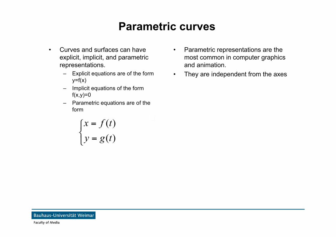
Parametric curves

• Curves and surfaces can haveexplicit, implicit, and parametricrepresentations.

– Explicit equations are of the formy=f(x)

– Implicit equations of the formf(x,y)=0

– Parametric equations are of theform

• Parametric representations are themost common in computer graphicsand animation.

• They are independent from the axes

!"#

=

=

)()(tgytfx

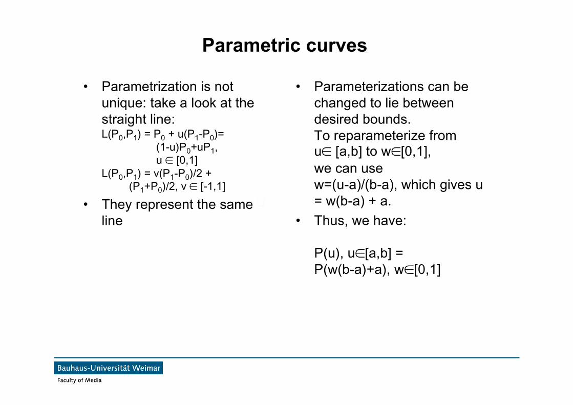
Parametric curves

• Parametrization is notunique: take a look at thestraight line:L(P0,P1) = P0 + u(P1-P0)= (1-u)P0+uP1, u ∈ [0,1]L(P0,P1) = v(P1-P0)/2 + (P1+P0)/2, v ∈ [-1,1]

• They represent the sameline

• Parameterizations can bechanged to lie betweendesired bounds.To reparameterize fromu∈ [a,b] to w∈[0,1],we can usew=(u-a)/(b-a), which gives u= w(b-a) + a.

• Thus, we have:

P(u), u∈[a,b] =P(w(b-a)+a), w∈[0,1]

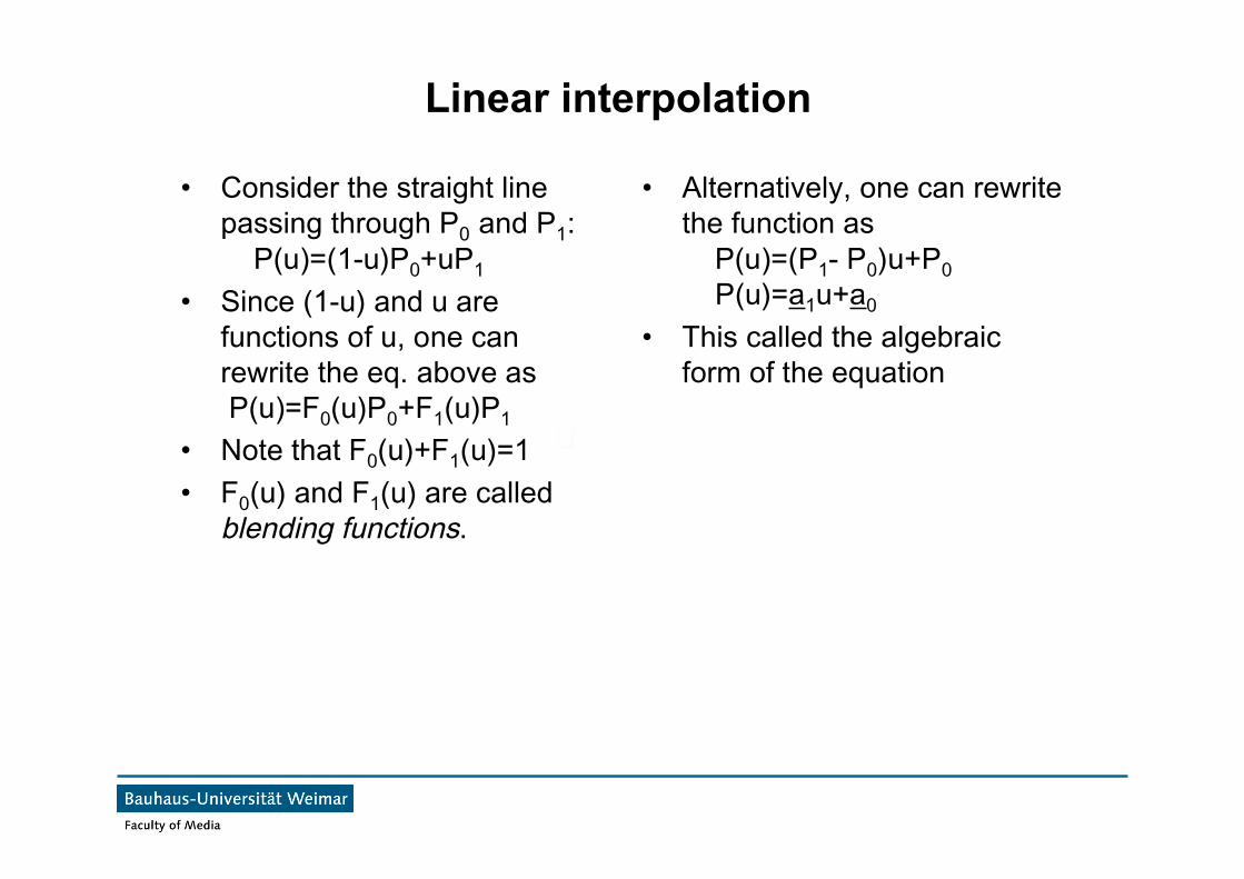
Linear interpolation

• Consider the straight linepassing through P0 and P1: P(u)=(1-u)P0+uP1

• Since (1-u) and u arefunctions of u, one canrewrite the eq. above as P(u)=F0(u)P0+F1(u)P1

• Note that F0(u)+F1(u)=1• F0(u) and F1(u) are calledblending functions.

• Alternatively, one can rewritethe function as P(u)=(P1- P0)u+P0 P(u)=a1u+a0

• This called the algebraicform of the equation

Linear interpolation

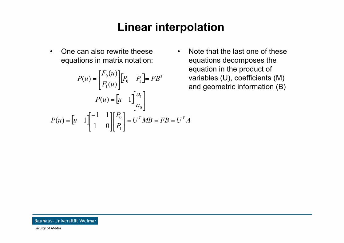
• One can also rewrite theeseequations in matrix notation:

• Note that the last one of theseequations decomposes theequation in the product ofvariables (U), coefficients (M)and geometric information (B)

[ ]

[ ]

[ ] AUFBMBUPP

uuP

aa

uuP

FBPPuFuF

uP

TT

T

===!"

#$%

&!"

#$%

&'=

!"

#$%

&=

=!"

#$%

&=

1

0

0

1

101

0

0111

1)(

1)(

)()(

)(

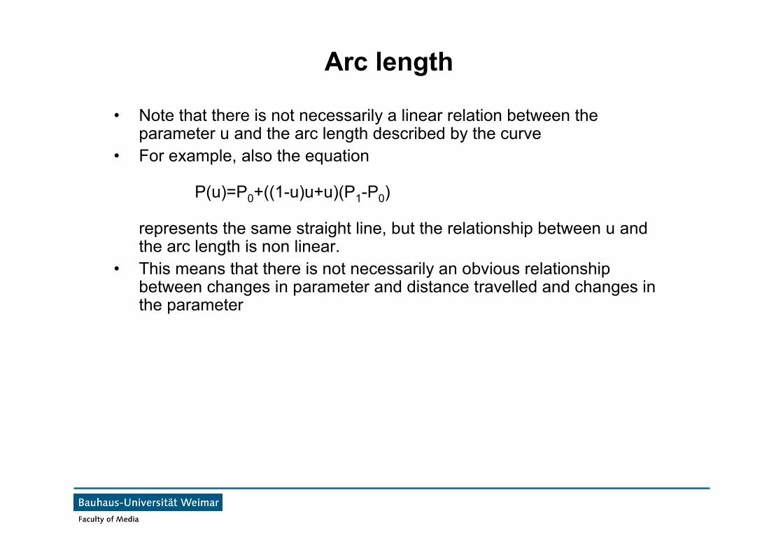
Arc length

• Note that there is not necessarily a linear relation between theparameter u and the arc length described by the curve

• For example, also the equation

P(u)=P0+((1-u)u+u)(P1-P0)

represents the same straight line, but the relationship between u andthe arc length is non linear.

• This means that there is not necessarily an obvious relationshipbetween changes in parameter and distance travelled and changes inthe parameter

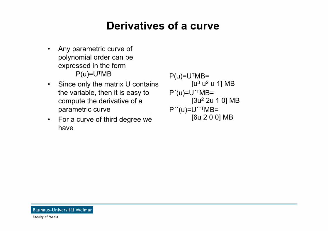
Derivatives of a curve

• Any parametric curve ofpolynomial order can beexpressed in the form P(u)=UTMB

• Since only the matrix U containsthe variable, then it is easy tocompute the derivative of aparametric curve

• For a curve of third degree wehave

P(u)=UTMB= [u3 u2 u 1] MB

P´(u)=U´TMB= [3u2 2u 1 0] MB

P´´(u)=U´´TMB= [6u 2 0 0] MB

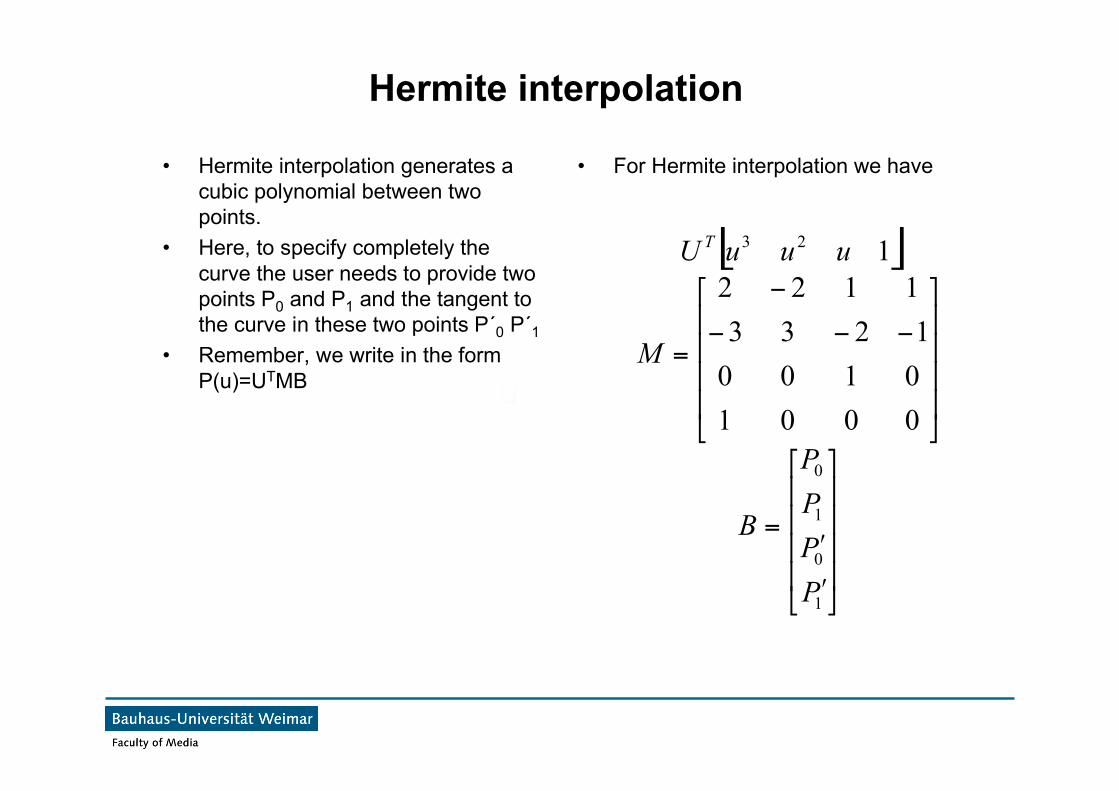
Hermite interpolation

• Hermite interpolation generates acubic polynomial between twopoints.

• Here, to specify completely thecurve the user needs to provide twopoints P0 and P1 and the tangent tothe curve in these two points P´0 P´1

• Remember, we write in the formP(u)=UTMB

• For Hermite interpolation we have

[ ]

!!!!

"

#

$$$$

%

&

'

'=

!!!!

"

#

$$$$

%

&

(((

(

=

1

0

1

0

23

0001010012331122

1

PPPP

B

M

uuuUT

Hermite interpolation

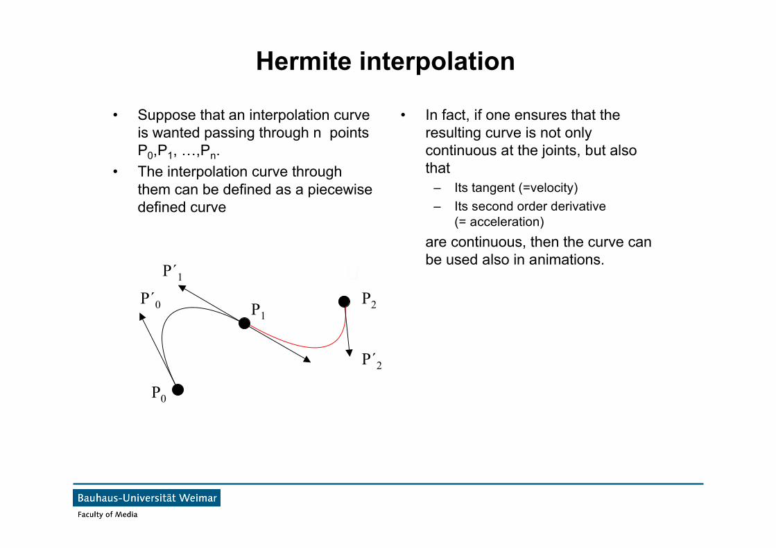
• Suppose that an interpolation curveis wanted passing through n pointsP0,P1, …,Pn.

• The interpolation curve throughthem can be defined as a piecewisedefined curve

• In fact, if one ensures that theresulting curve is not onlycontinuous at the joints, but alsothat

– Its tangent (=velocity)– Its second order derivative

(= acceleration) are continuous, then the curve can

be used also in animations.

P0

P1

P´1

P´0

P´2

P2

Continuity: parametric and geometric

• For a piecewise defined curve, there are two main ways of defining thecontinuity at the borders of the single intervals of definition– 1st order parametric continuity (C1): the end tangent vector at the two ends

must be exactly the same– 1st order geometric continuity (G1): the direction of the tangent must be the

same, but the magnitudes may differ– Similar definitions for higher oder continuity (C2-G2)

• Parametric continuity is sensitive to the „velocity“ of the parameter onthe curve, geometric continuity is not

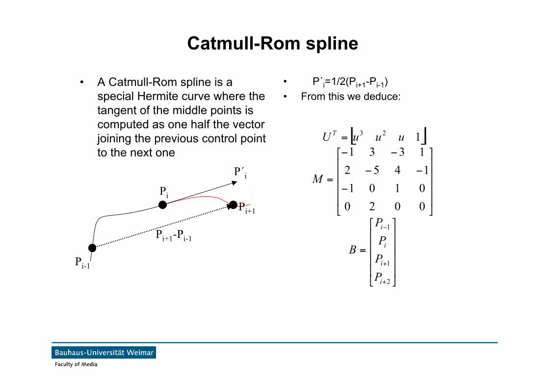
Catmull-Rom spline

• A Catmull-Rom spline is aspecial Hermite curve where thetangent of the middle points iscomputed as one half the vectorjoining the previous control pointto the next one

• P´i=1/2(Pi+1-Pi-1)• From this we deduce:

Pi-1

Pi

P´i

Pi+1-Pi-1

Pi+1

[ ]

!!!!

"

#

$$$$

%

&

=

!!!!

"

#

$$$$

%

&

'

''

''

=

=

+

+

'

2

1

1

23

00200101145213311

i

i

i

i

T

PPPP

B

M

uuuU

Catmull-Rom spline

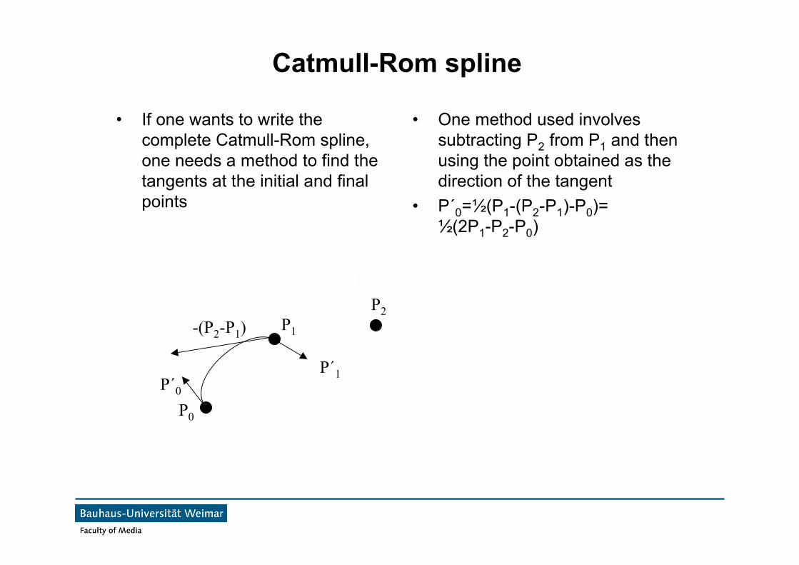
• If one wants to write thecomplete Catmull-Rom spline,one needs a method to find thetangents at the initial and finalpoints

• One method used involvessubtracting P2 from P1 and thenusing the point obtained as thedirection of the tangent

• P´0=½(P1-(P2-P1)-P0)=½(2P1-P2-P0)

P0

P1

P´1P´0

P2-(P2-P1)

Catmull-Rom spline

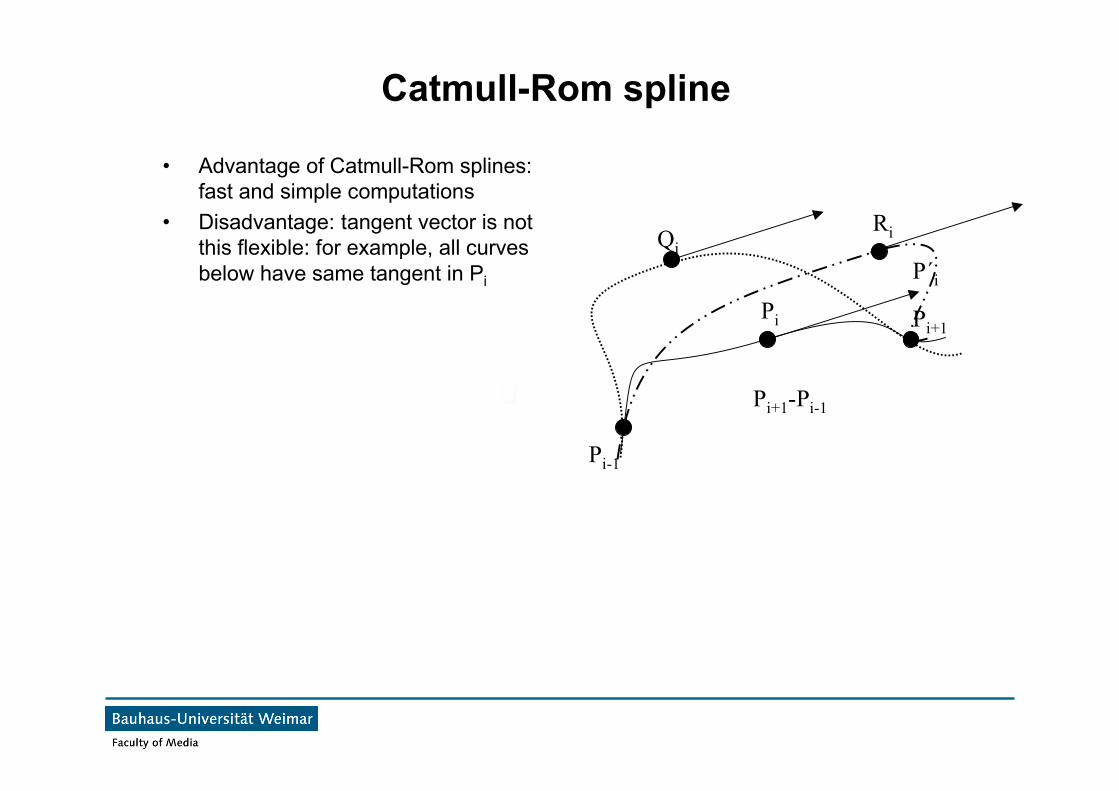
• Advantage of Catmull-Rom splines:fast and simple computations

• Disadvantage: tangent vector is notthis flexible: for example, all curvesbelow have same tangent in Pi

Pi-1

Pi

P´i

Pi+1-Pi-1

Pi+1

QiRi

Catmull-Rom spline

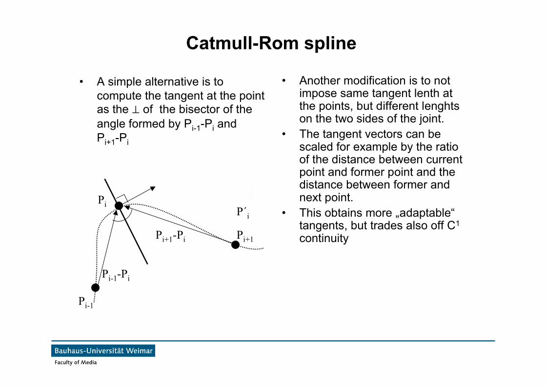
• A simple alternative is tocompute the tangent at the pointas the ⊥ of the bisector of theangle formed by Pi-1-Pi andPi+1-Pi

• Another modification is to notimpose same tangent lenth atthe points, but different lenghtson the two sides of the joint.

• The tangent vectors can bescaled for example by the ratioof the distance between currentpoint and former point and thedistance between former andnext point.

• This obtains more „adaptable“tangents, but trades also off C1

continuity

Pi-1

PiP´i

Pi+1-Pi Pi+1

Pi-1-Pi

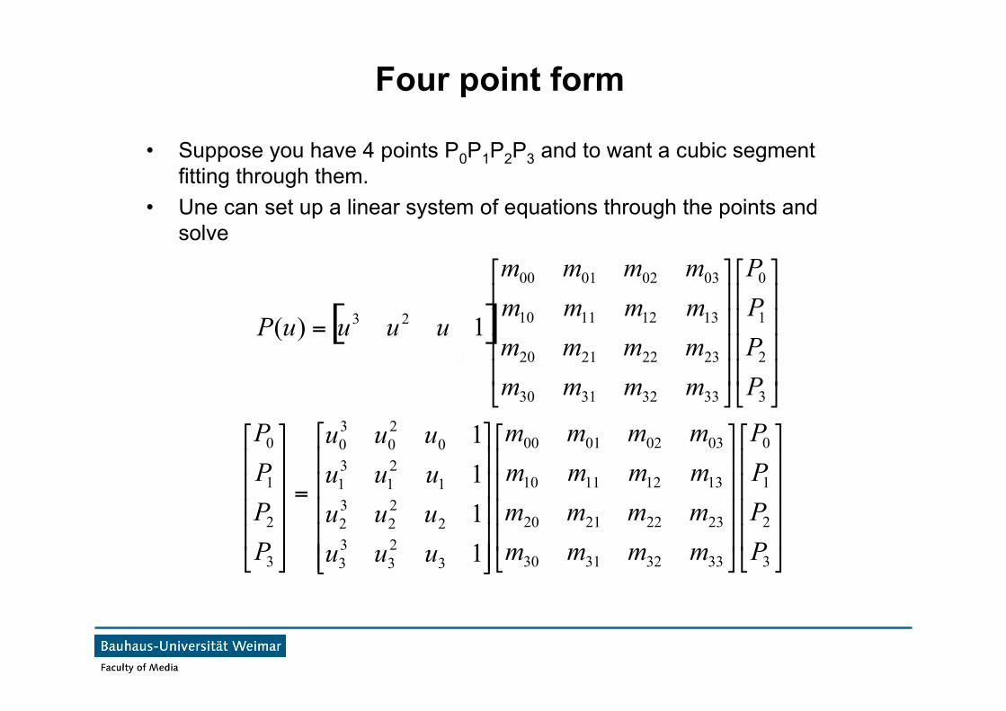
Four point form

• Suppose you have 4 points P0P1P2P3 and to want a cubic segmentfitting through them.

• Une can set up a linear system of equations through the points andsolve

[ ]!!!!

"

#

$$$$

%

&

!!!!

"

#

$$$$

%

&

=

3

2

1

0

33323130

23222120

13121110

03020100

23 1)(

PPPP

mmmmmmmmmmmmmmmm

uuuuP

!!!!

"

#

$$$$

%

&

!!!!

"

#

$$$$

%

&

!!!!!

"

#

$$$$$

%

&

=

!!!!

"

#

$$$$

%

&

3

2

1

0

33323130

23222120

13121110

03020100

323

33

222

32

121

31

020

30

3

2

1

0

1111

PPPP

mmmmmmmmmmmmmmmm

uuuuuuuuuuuu

PPPP

Four point form

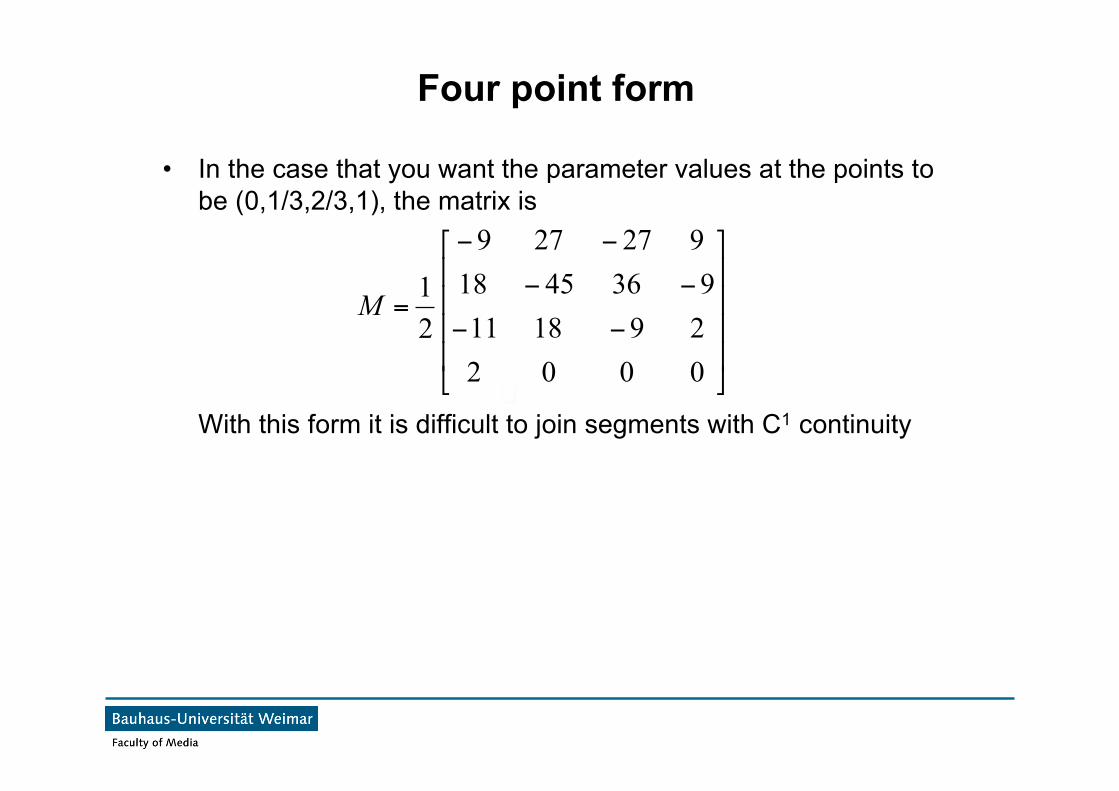
• In the case that you want the parameter values at the points tobe (0,1/3,2/3,1), the matrix is

With this form it is difficult to join segments with C1 continuity

!!!!

"

#

$$$$

%

&

''

''

''

=

00022918119364518927279

21M

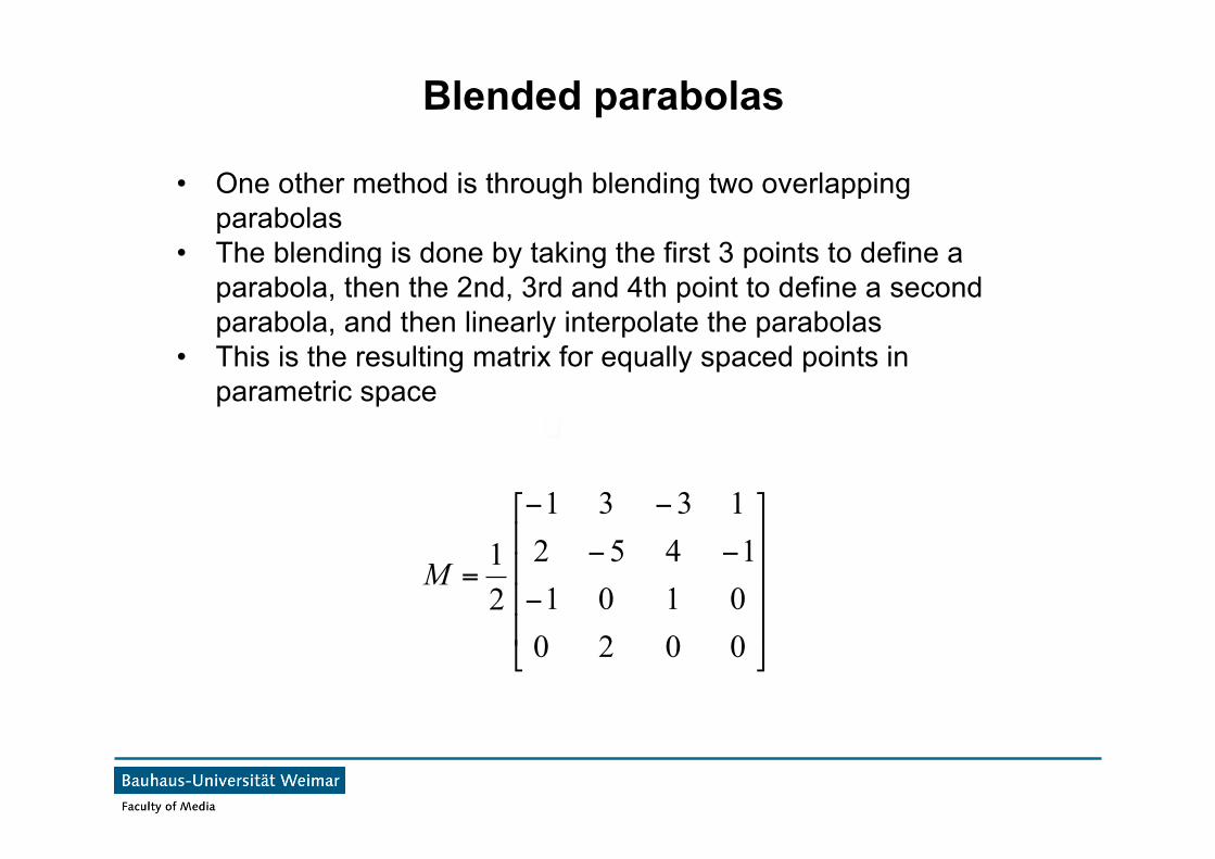
Blended parabolas

• One other method is through blending two overlappingparabolas

• The blending is done by taking the first 3 points to define aparabola, then the 2nd, 3rd and 4th point to define a secondparabola, and then linearly interpolate the parabolas

• This is the resulting matrix for equally spaced points inparametric space

!!!!

"

#

$$$$

%

&

'

''

''

=

0020010114521331

21M

Bezier curves

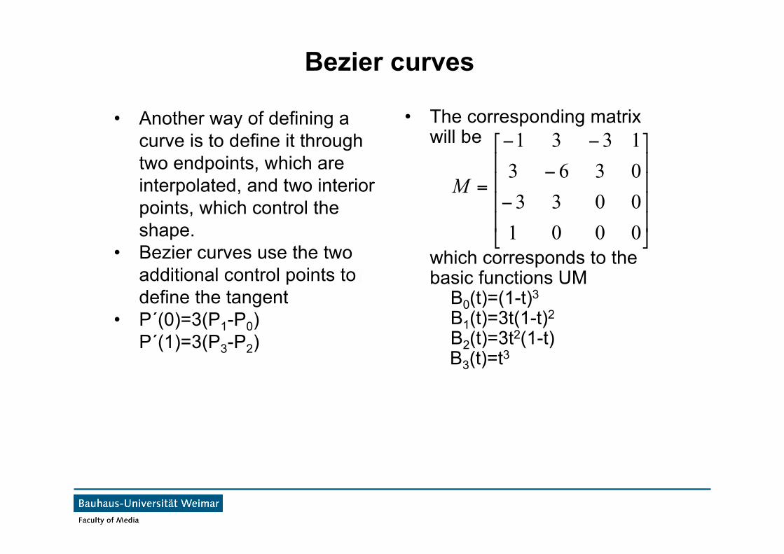
• Another way of defining acurve is to define it throughtwo endpoints, which areinterpolated, and two interiorpoints, which control theshape.

• Bezier curves use the twoadditional control points todefine the tangent

• P´(0)=3(P1-P0)P´(1)=3(P3-P2)

• The corresponding matrixwill be

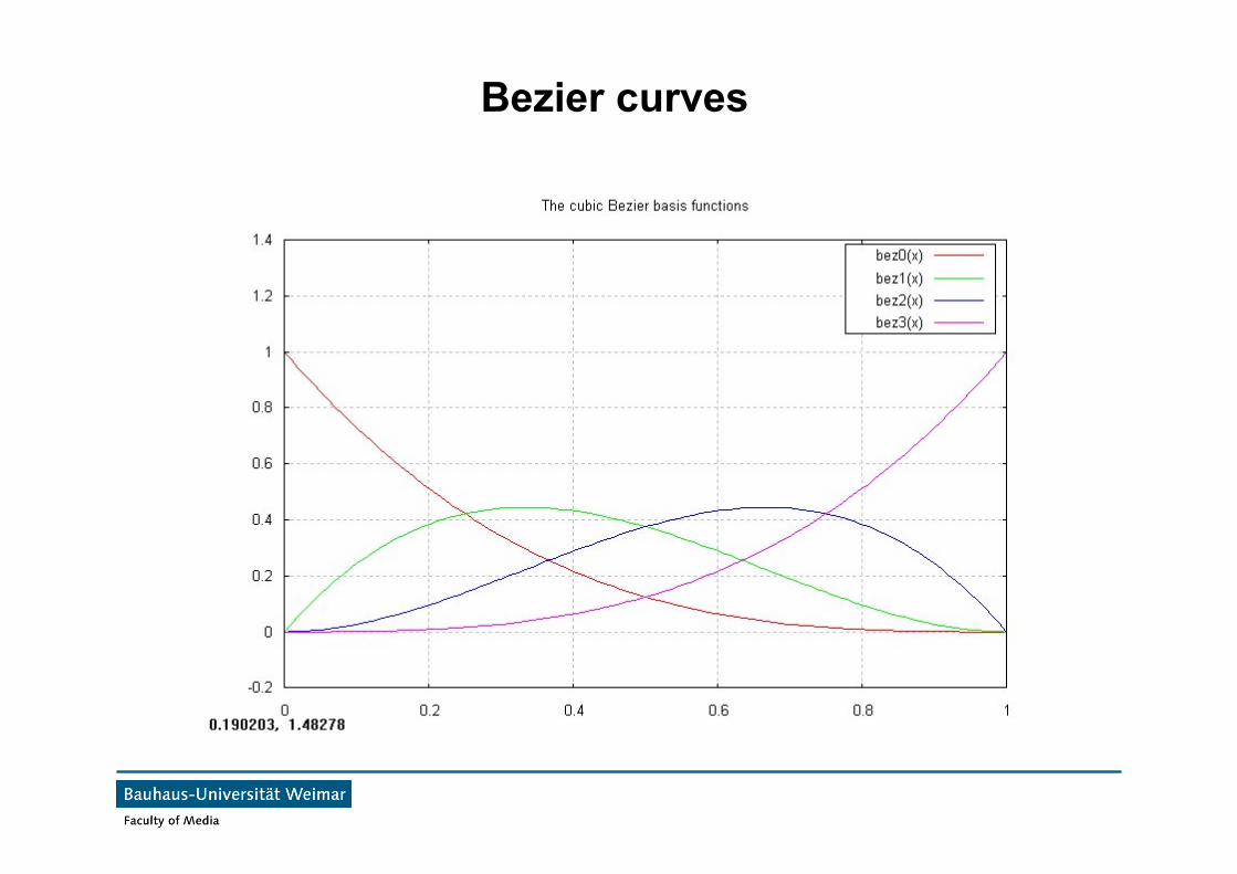
which corresponds to thebasic functions UM B0(t)=(1-t)3

B1(t)=3t(1-t)2

B2(t)=3t2(1-t) B3(t)=t3

!!!!

"

#

$$$$

%

&

'

'

''

=

0001003303631331

M

Bezier curves

Bezier curves

• In fact, Bezier curves can be of any order. The basis functionsare

Bin(t)=ti(1-t)n-in!/i!/(n-i)!

Where n is the degree and i=0,…,n.• And the Bezier curve passing through the points P0,P1,…,Pn is

Q(T)=Σi=0,…,nBin(t)Pi

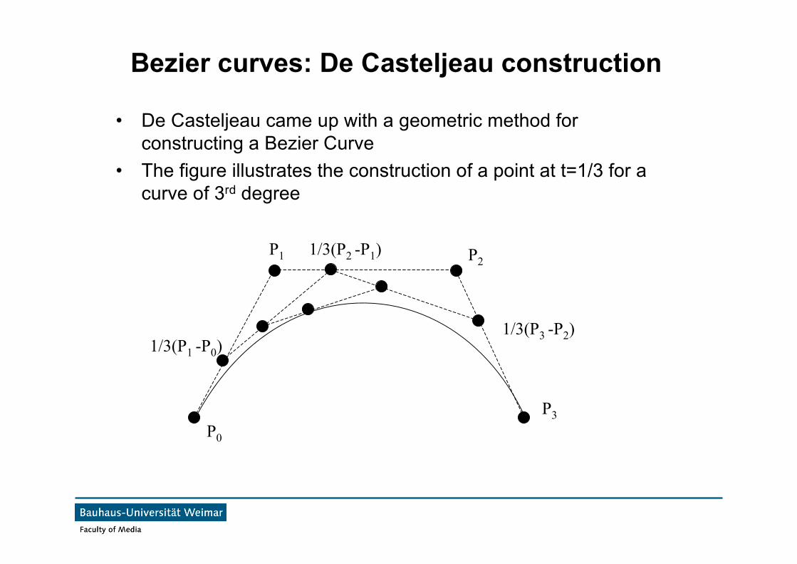
Bezier curves: De Casteljeau construction

• De Casteljeau came up with a geometric method forconstructing a Bezier Curve

• The figure illustrates the construction of a point at t=1/3 for acurve of 3rd degree

P0

P1 P2

P3

1/3(P1 -P0)

1/3(P2 -P1)

1/3(P3 -P2)

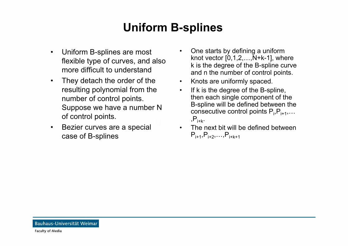
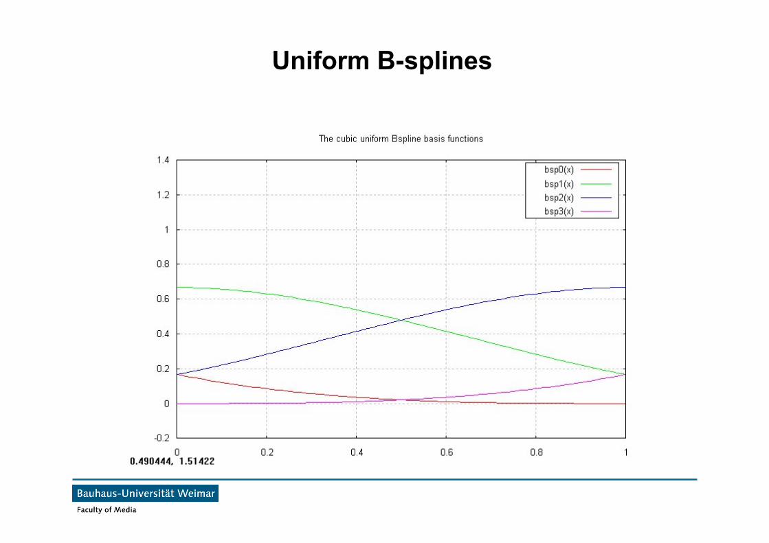
Uniform B-splines

• Uniform B-splines are mostflexible type of curves, and alsomore difficult to understand

• They detach the order of theresulting polynomial from thenumber of control points.Suppose we have a number Nof control points.

• Bezier curves are a specialcase of B-splines

• One starts by defining a uniformknot vector [0,1,2,…,N+k-1], wherek is the degree of the B-spline curveand n the number of control points.

• Knots are uniformly spaced.• If k is the degree of the B-spline,

then each single component of theB-spline will be defined between theconsecutive control points Pi,Pi+1,…,Pi+k.

• The next bit will be defined betweenPi+1,Pi+2,…,Pi+k+1

Uniform B-splines

• The equation for k-order B-splinewith N+1 control points(P0 , P1 , ... , PN ) is

P(t) = Σi=0,..,N Ni,k(t) Pi , tk-1 <= t <= tN+1

• In a B-spline each control point isassociated with a basis function Ni,kwhich is given by the recurrencerelations Ni,k(t) = Ni,k-1(t) (t - ti)/(ti+k-1 - ti) + Ni+1,k-1(t) (ti+k - t)/(ti+k - ti+1), Ni,1 = {1 if ti <= t <=ti+1, 0 otherwise }

• Ni,k is a polynomial of order k(degree k-1) on each interval ti <t < ti+1.

• k must be at least 2 (linear) andcan be not more, than n+1 (thenumber of control points).

• A knot vector(t0,t1,..., tN+k) mustbe specified. Across the knotsbasis functions are C k-2

continuous.

Uniform B-splines

• B-spline basis functions likeBezier ones are nonnegativeNi,k ≥ 0 and have "partition ofunity" property

Σi=0,N Ni,k(t) = 1, tk-1 < t < tn+1

therefore

0 ≤ Ni,k ≤ 1.

• Since Ni,k = 0 for t ≤ ti or t ≥ ti+k,a control point Pi influences thecurve only for ti < t < ti+k.

B-splines

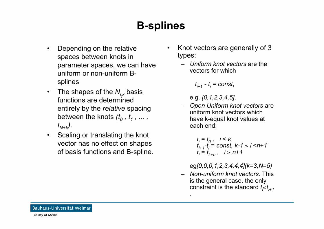
• Depending on the relativespaces between knots inparameter spaces, we can haveuniform or non-uniform B-splines

• The shapes of the Ni,k basisfunctions are determinedentirely by the relative spacingbetween the knots (t0 , t1 , ... ,tN+k).

• Scaling or translating the knotvector has no effect on shapesof basis functions and B-spline.

• Knot vectors are generally of 3types:– Uniform knot vectors are the

vectors for which

ti+1 - ti = const,

e.g. [0,1,2,3,4,5].– Open Uniform knot vectors are

uniform knot vectors whichhave k-equal knot values ateach end:

ti = t0 , i < k ti+1-ti = const, k-1 ≤ i <n+1 ti = tk+n , i ≥ n+1

eg[0,0,0,1,2,3,4,4,4](k=3,N=5)– Non-uniform knot vectors. This

is the general case, the onlyconstraint is the standard ti≤ti+1.

B-splines

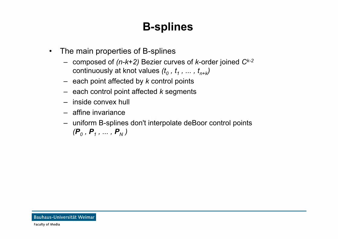
• The main properties of B-splines– composed of (n-k+2) Bezier curves of k-order joined Ck-2

continuously at knot values (t0 , t1 , ... , tn+k)– each point affected by k control points– each control point affected k segments– inside convex hull– affine invariance– uniform B-splines don't interpolate deBoor control points

(P0 , P1 , ... , PN )

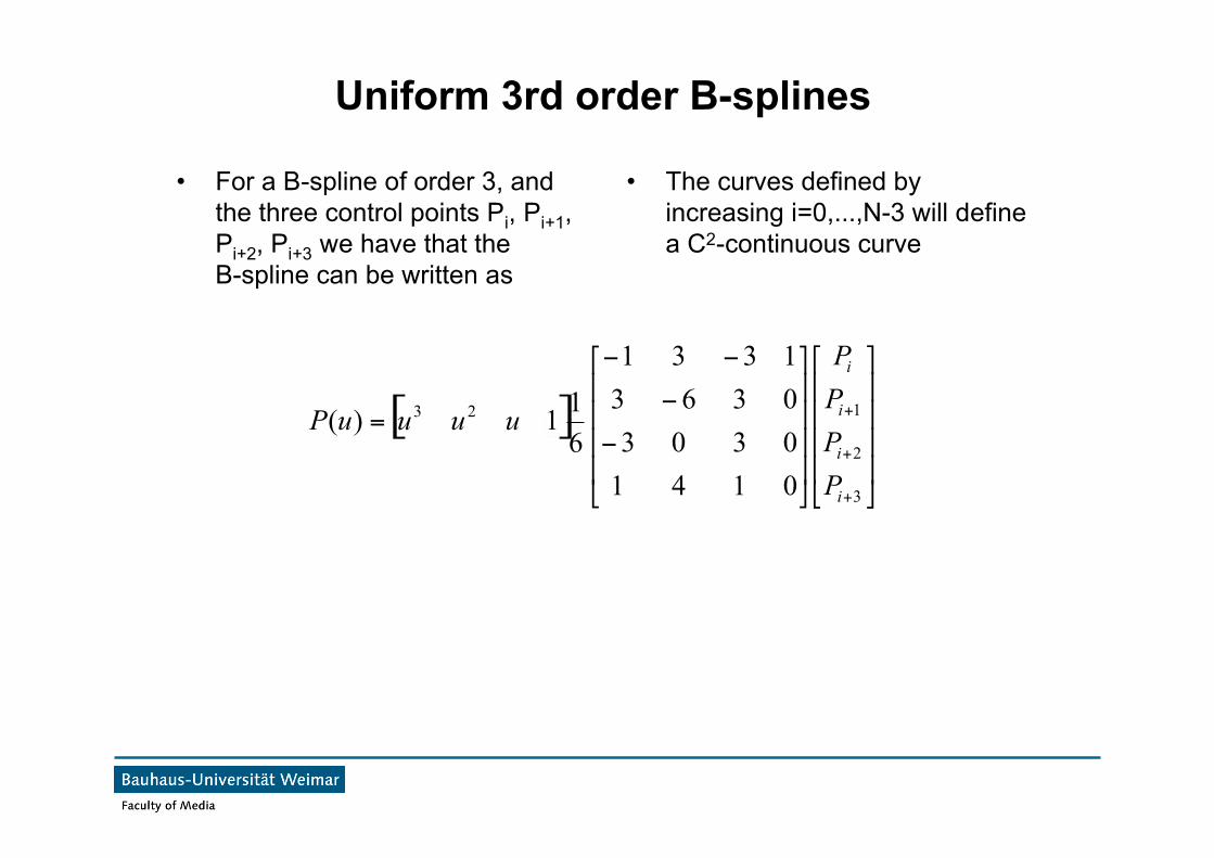
Uniform 3rd order B-splines

• For a B-spline of order 3, andthe three control points Pi, Pi+1,Pi+2, Pi+3 we have that theB-spline can be written as

• The curves defined byincreasing i=0,...,N-3 will definea C2-continuous curve

[ ]!!!!

"

#

$$$$

%

&

!!!!

"

#

$$$$

%

&

'

'

''

=

+

+

+

3

2

123

0141030303631331

611)(

i

i

i

i

PPPP

uuuuP

Uniform B-splines

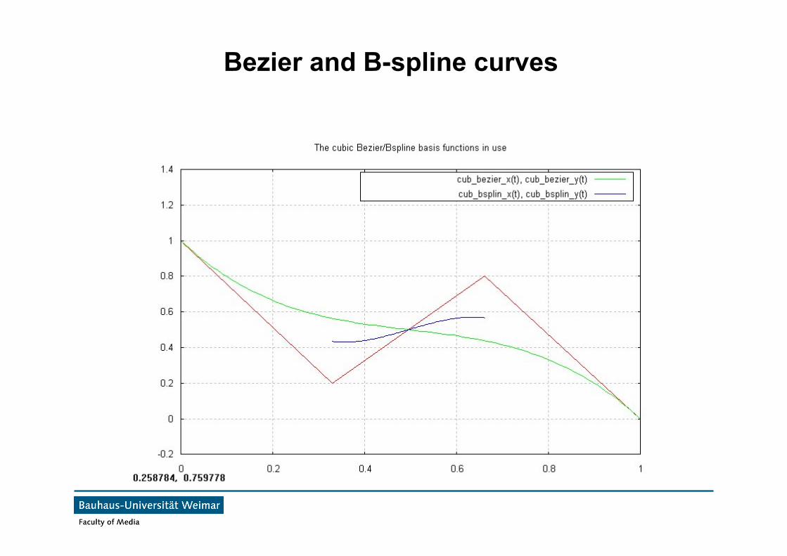
Bezier and B-spline curves

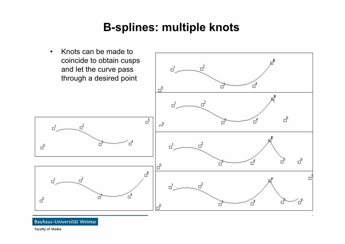
B-splines: multiple knots

• Knots can be made tocoincide to obtain cuspsand let the curve passthrough a desired point

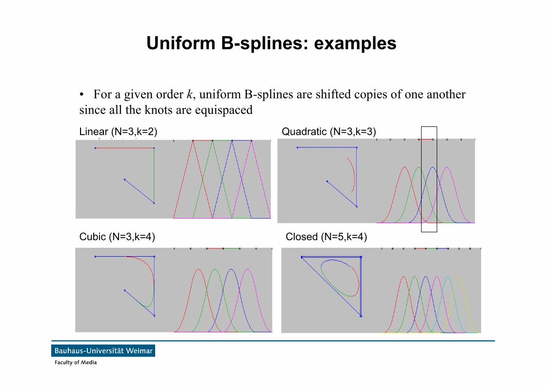
• For a given order k, uniform B-splines are shifted copies of one anothersince all the knots are equispaced

Uniform B-splines: examples

Linear (N=3,k=2) Quadratic (N=3,k=3)

Cubic (N=3,k=4) Closed (N=5,k=4)

NURBS

• Stands for non-uniform rational B-splines– Non-uniform: knots are not at same distance– Rational: it‘s a fraction, with B-splines at the numerator and

denominator• Advantages: one can express circular arcs with NURBS• Disadvantages: lots of computational effort

NURBS

• Recall that the B-spline is weightedsum of its control points

P(t) = Σi=0,..,N Ni,k(t) Pi , tk-1 ≤ t ≤ tN+1

and the weights Ni,k have the"partition of unity" property

Σi=0,..,N Ni,k(t) = 1 .

• As weights Ni,k depend on the knotvector only, it is useful to add toevery control point one more weightwi which can be set independently

P(t)=Σi=0,..,NwiNi,k(t)Pi/Σi=0,..,NwiNi,k(t) .

• Increasing a weight wimakes the point moreinfluence and attracts thecurve to it.

• The denominator in the 2nd

equation normalizes weights,so we will get the 1st

equation if we setwi = const for all i.

• Full weights wiNi,k satisfy the"partition of unity" conditionagain.

Global vs local control

• Depending on the curve formulation, moving a control point can havedifferent effects– Local control: in this case the effect of the movement is limited in its

influence along the curve– Global control: moving a point redefines the whole curve

• Local control is the most desirable for manipulating a curve• Almost all of the piecewise defined curves have local control• Only exception: Hermite curves enforcing C2 continuity

Modeling with splines

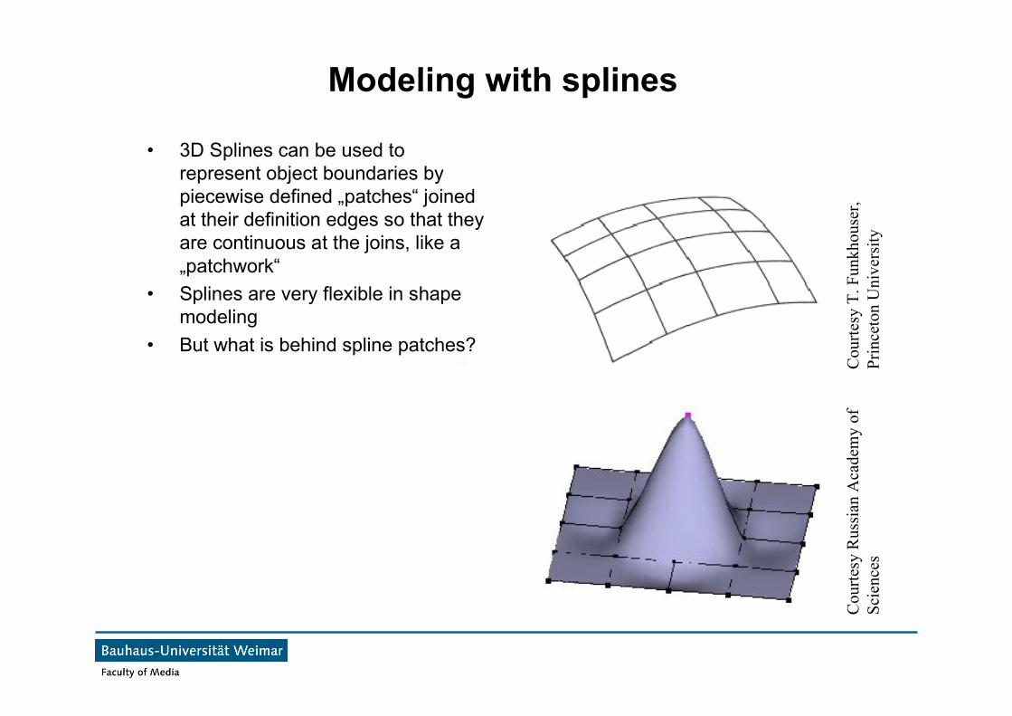
• 3D Splines can be used torepresent object boundaries bypiecewise defined „patches“ joinedat their definition edges so that theyare continuous at the joins, like a„patchwork“

• Splines are very flexible in shapemodeling

• But what is behind spline patches?

Cou

rtesy

T. F

unkh

ouse

r,Pr

ince

ton

Uni

vers

ityC

ourte

sy R

ussi

an A

cade

my

ofSc

ienc

es

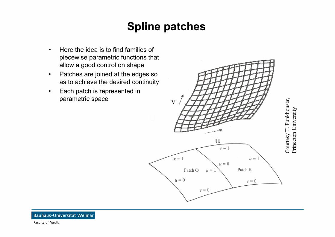
Spline patches

• Here the idea is to find families ofpiecewise parametric functions thatallow a good control on shape

• Patches are joined at the edges soas to achieve the desired continuity

• Each patch is represented inparametric space

Cou

rtesy

T. F

unkh

ouse

r,Pr

ince

ton

Uni

vers

ity

Spline patches

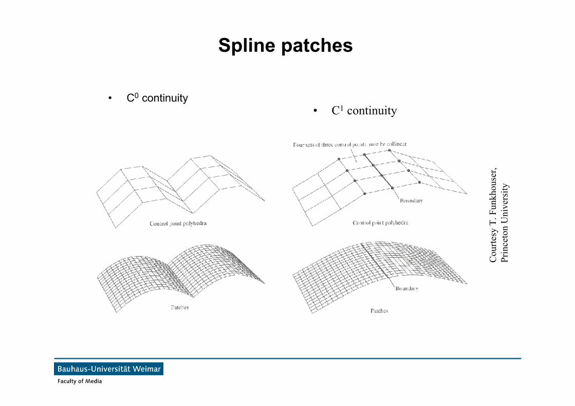
• C0 continuity

Cou

rtesy

T. F

unkh

ouse

r,Pr

ince

ton

Uni

vers

ity

• C1 continuity

Spline patches

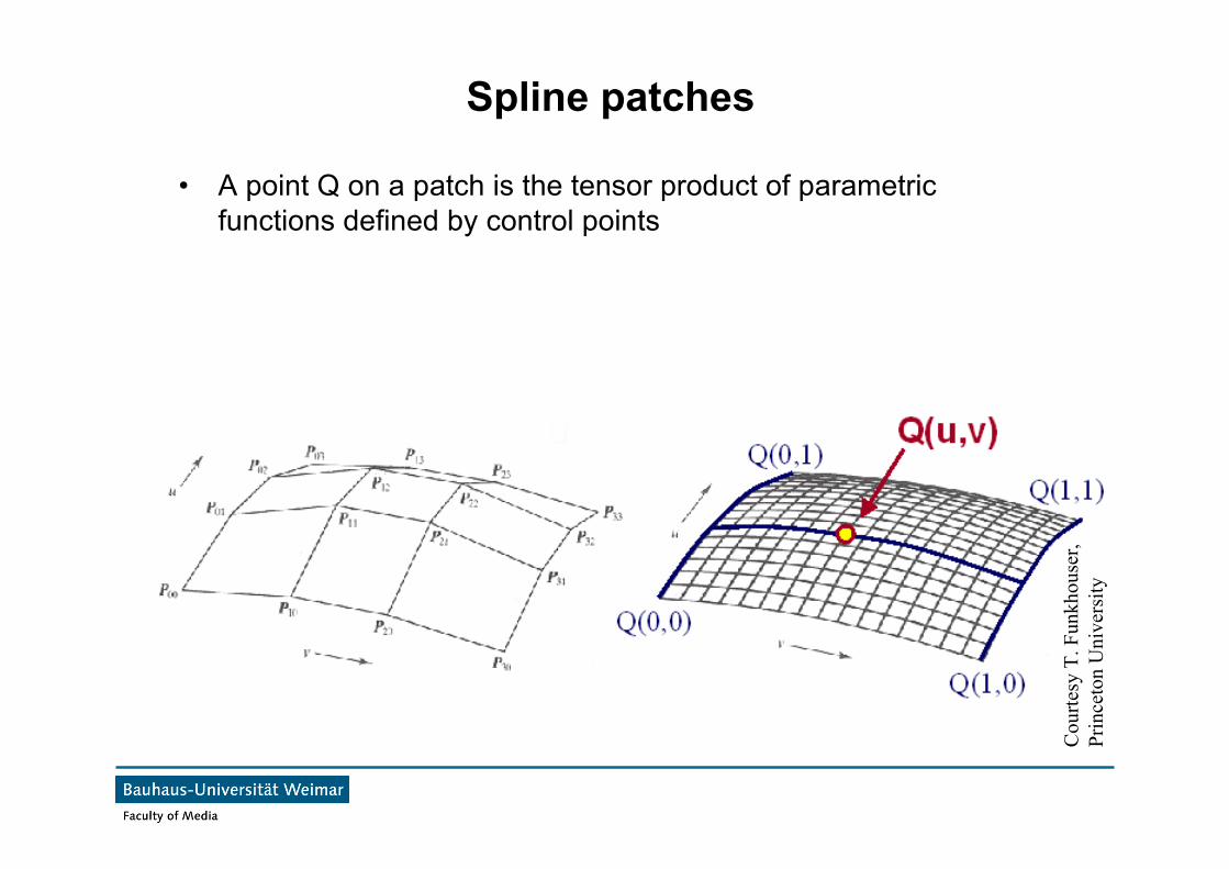
• A point Q on a patch is the tensor product of parametricfunctions defined by control points

Cou

rtesy

T. F

unkh

ouse

r,Pr

ince

ton

Uni

vers

ity

Spline patches

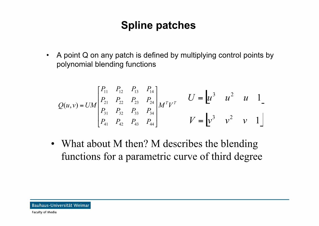
• A point Q on any patch is defined by multiplying control points bypolynomial blending functions

TTVM

PPPPPPPPPPPPPPPP

UMvuQ!!!!

"

#

$$$$

%

&

=

44434241

34333231

24232221

14131211

),([ ]123 uuuU =

[ ]123 vvvV =

• What about M then? M describes the blendingfunctions for a parametric curve of third degree

Spline patches

!!!!

"

#

$$$$

%

&

'

'

''

='

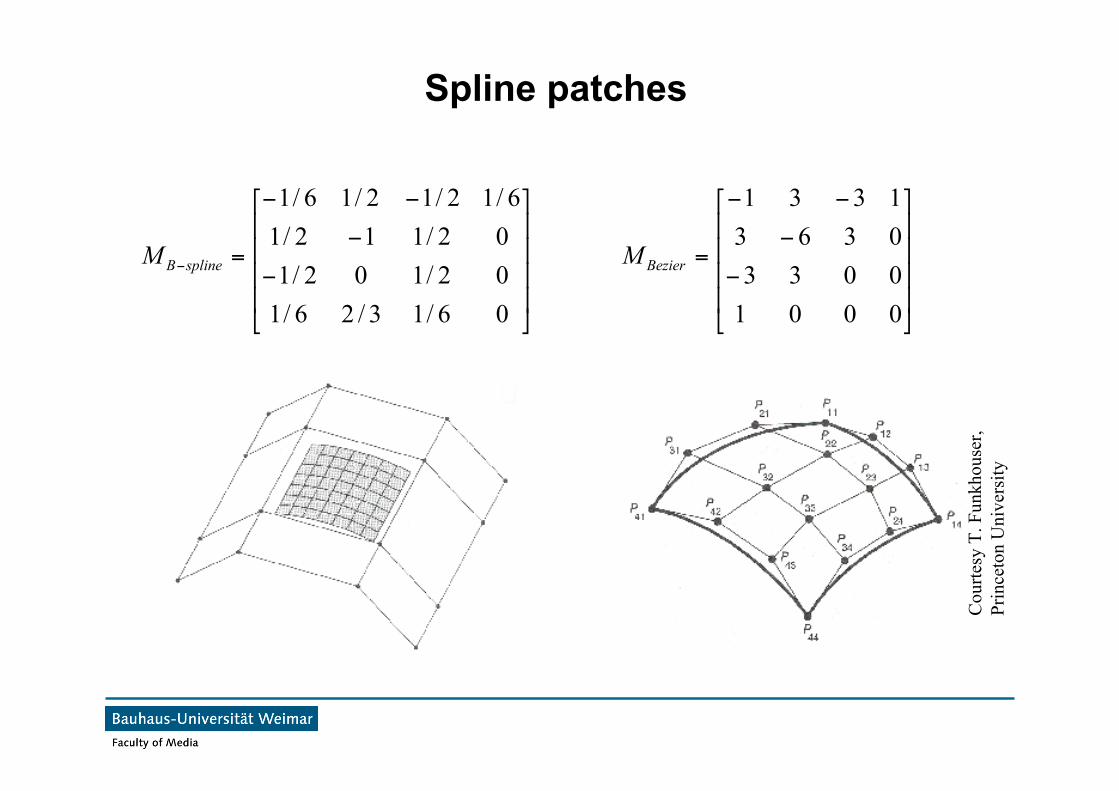
06/13/26/102/102/102/112/16/12/12/16/1

splineBM

!!!!

"

#

$$$$

%

&

'

'

''

=

0001003303631331

BezierM

Cou

rtesy

T. F

unkh

ouse

r,Pr

ince

ton

Uni

vers

ity

Spline patches

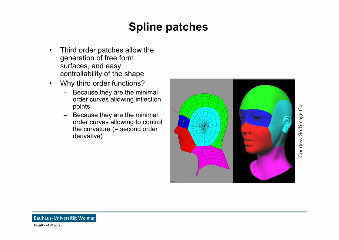
• Third order patches allow thegeneration of free formsurfaces, and easycontrollability of the shape

• Why third order functions?– Because they are the minimal

order curves allowing inflectionpoints

– Because they are the minimalorder curves allowing to controlthe curvature (= second orderderivative)

Cou

rtesy

Sof

timag

e C

o.

Charles A. Wüthrich

+++ Ende - The end - Finis - Fin - Fine +++ Ende - The end - Finis - Fin - Fine +++

End

Cop

yrig

ht (c

) 198

8 IL

M