Embed Size (px)
Citation preview
1
Mirko Guarnera
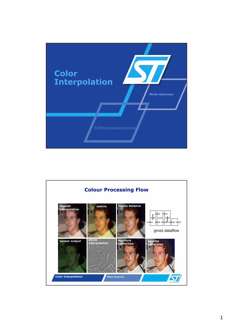
Color Interpolation
STMicroelectronics
Color Interpolation Mirko Guarnera
Colour Processing Flow
smooth interpolation
sharp interpolation
colour balancematrix
sensor output aperture correction
gamma correction
gross dataflow
2
Color Interpolation Mirko Guarnera
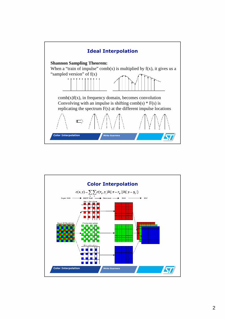
Ideal Interpolation
Shannon Sampling Theorem:When a “train of impulse” comb(x) is multiplied by f(x), it gives us a “sampled version” of f(x)
comb(x)f(x), in frequency domain, becomes convolutionConvolving with an impulse is shifting comb(s) * F(s) is replicating the spectrum F(s) at the different impulse locations
Color Interpolation Mirko Guarnera
Color Interpolation
3
Color Interpolation Mirko Guarnera
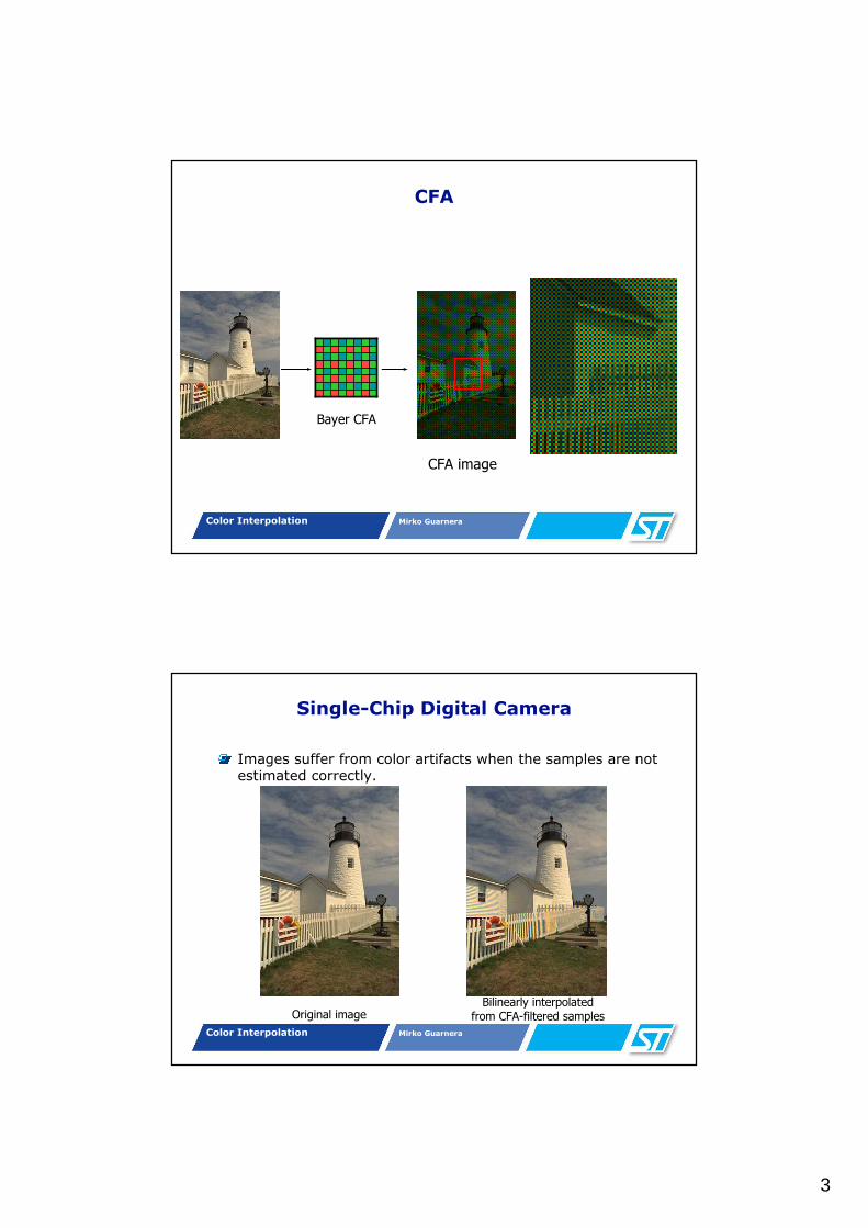
CFA
Bayer CFA
CFA image
Color Interpolation Mirko Guarnera
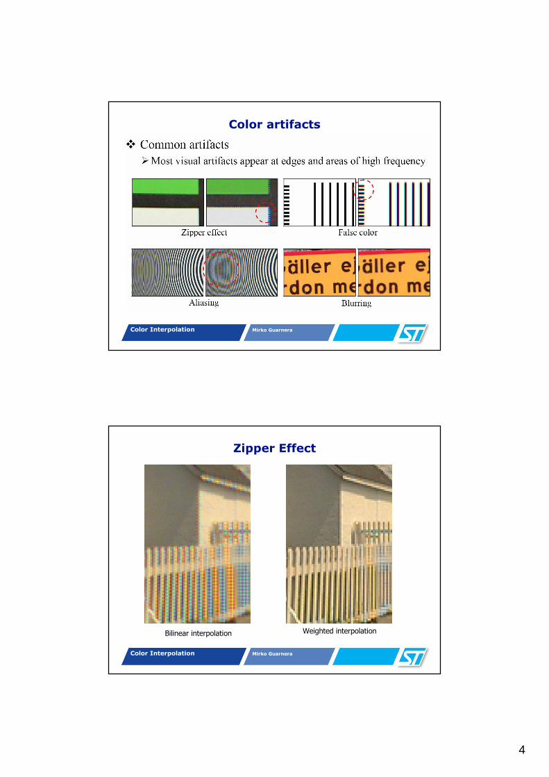
Single-Chip Digital Camera
Images suffer from color artifacts when the samples are not estimated correctly.
Original imageBilinearly interpolated from CFA-filtered samples
4
Color Interpolation Mirko Guarnera
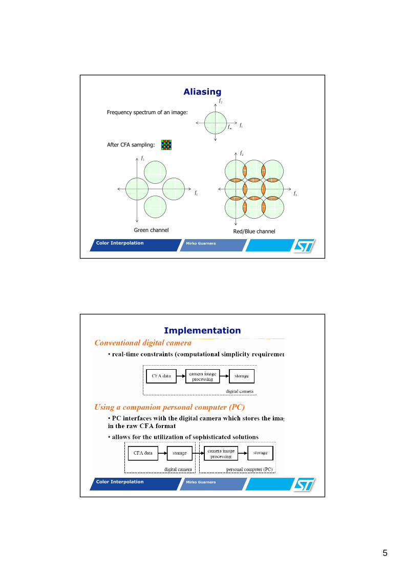
Color artifacts
Color Interpolation Mirko Guarnera
Zipper Effect
Bilinear interpolation Weighted interpolation
5
Color Interpolation Mirko Guarnera
Aliasing
mf 1f
2f
2f
1f
2f
1f
Green channel Red/Blue channel
Frequency spectrum of an image:
After CFA sampling:
Color Interpolation Mirko Guarnera
Implementation
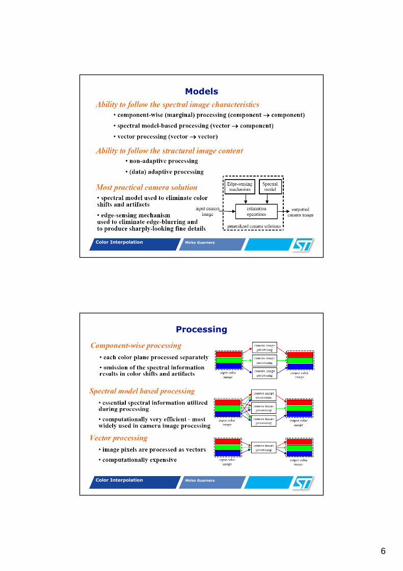
6
Color Interpolation Mirko Guarnera
Models
Color Interpolation Mirko Guarnera
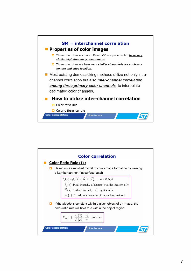
Processing
7
Color Interpolation Mirko Guarnera
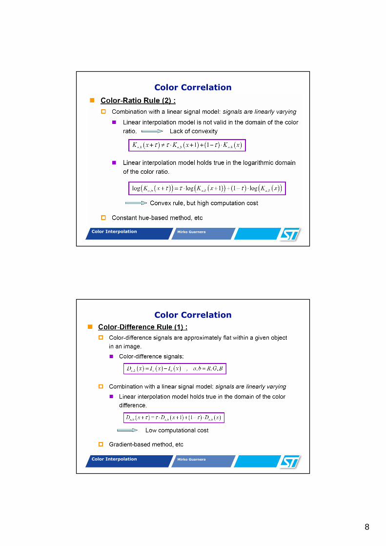
SM = interchannel correlation
Color Interpolation Mirko Guarnera
Color correlation
8
Color Interpolation Mirko Guarnera
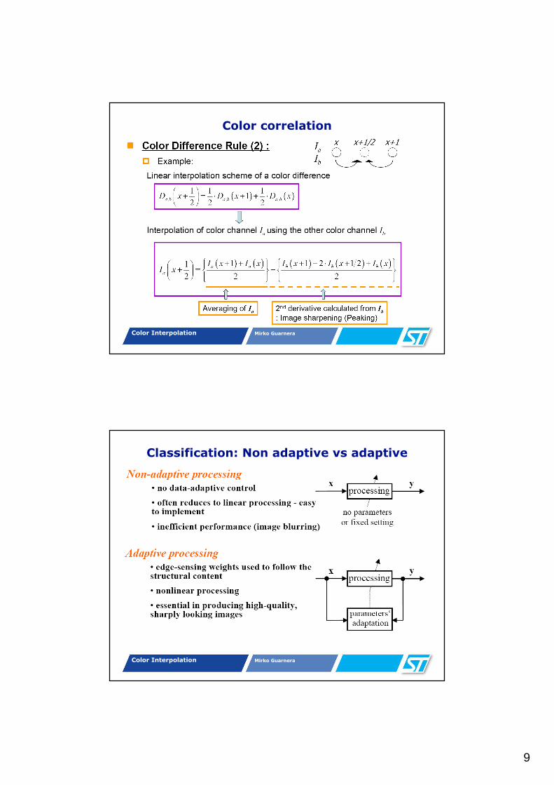
Color Correlation
Color Interpolation Mirko Guarnera
Color Correlation
9
Color Interpolation Mirko Guarnera
Color correlation
Color Interpolation Mirko Guarnera
Classification: Non adaptive vs adaptive
10
Color Interpolation Mirko Guarnera
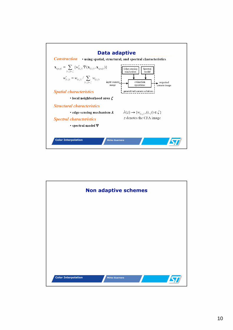
Data adaptive
Color Interpolation Mirko Guarnera
Non adaptive schemes
11
Color Interpolation Mirko Guarnera
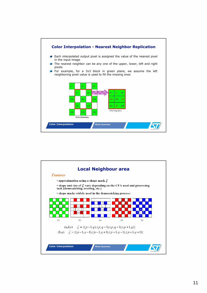
Color Interpolation - Nearest Neighbor Replication
Each interpolated output pixel is assigned the value of the nearest pixel in the input image
The nearest neighbor can be any one of the upper, lower, left and right pixels
For example, for a 3x3 block in green plane, we assume the left neighboring pixel value is used to fill the missing ones
Color Interpolation Mirko Guarnera
Local Neighbour area
12
Color Interpolation Mirko Guarnera
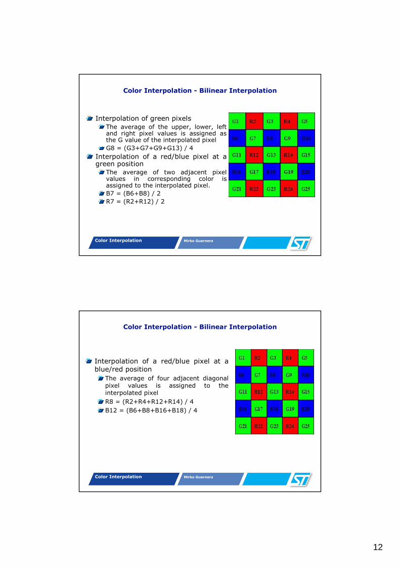
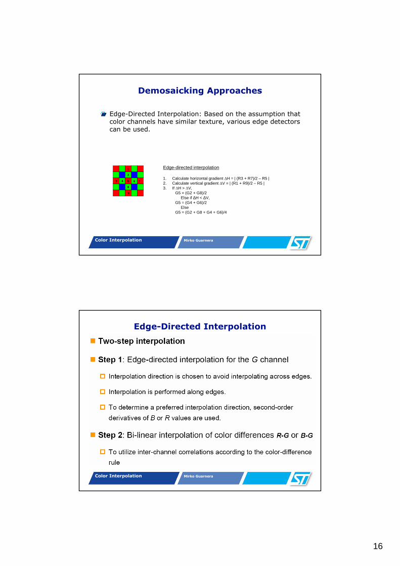
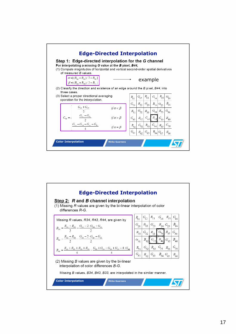
Color Interpolation - Bilinear Interpolation
Interpolation of green pixels
The average of the upper, lower, left and right pixel values is assigned as the G value of the interpolated pixel
G8 = (G3+G7+G9+G13) / 4
Interpolation of a red/blue pixel at a green position
The average of two adjacent pixel values in corresponding color is assigned to the interpolated pixel.
B7 = (B6+B8) / 2
R7 = (R2+R12) / 2
Color Interpolation Mirko Guarnera
Color Interpolation - Bilinear Interpolation
Interpolation of a red/blue pixel at a blue/red position
The average of four adjacent diagonal pixel values is assigned to the interpolated pixel
R8 = (R2+R4+R12+R14) / 4
B12 = (B6+B8+B16+B18) / 4
13
Color Interpolation Mirko Guarnera
Bilinear
Color Interpolation Mirko Guarnera
Adaptive schemes
14
Color Interpolation Mirko Guarnera
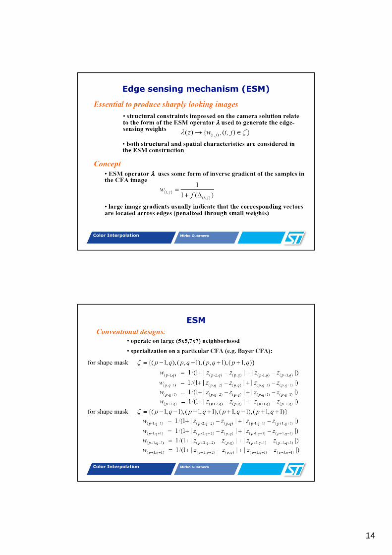
Edge sensing mechanism (ESM)
Color Interpolation Mirko Guarnera
ESM
15
Color Interpolation Mirko Guarnera
ESM
Color Interpolation Mirko Guarnera
Edge SensingInterpolation of green pixels :
First, define two gradients, one in horizontal direction, the other in vertical direction, for each blue/red position. For instance,consider B8 : define two gradients as
Define some threshold value T The algorithm then can be described as:
The choice of T depends on the images and can have defferentoptimum values from different neighborhoods. A particular choice of T is
16
Color Interpolation Mirko Guarnera
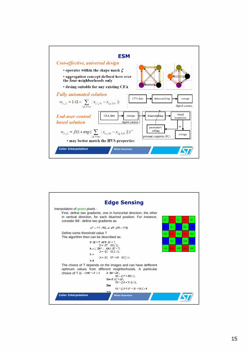
Demosaicking Approaches
Edge-Directed Interpolation: Based on the assumption that color channels have similar texture, various edge detectors can be used.
Edge-directed interpolation
1. Calculate horizontal gradient ∆H = | (R3 + R7)/2 – R5 | 2. Calculate vertical gradient ∆V = | (R1 + R9)/2 – R5 | 3. If ∆H > ∆V,
G5 = (G2 + G8)/2Else if ∆H < ∆V,
G5 = (G4 + G6)/2 Else
G5 = (G2 + G8 + G4 + G6)/4
1
2
4 5 6 7
8
9
3
Color Interpolation Mirko Guarnera
Edge-Directed Interpolation
17
Color Interpolation Mirko Guarnera
Edge-Directed Interpolation
example
Color Interpolation Mirko Guarnera
Edge-Directed Interpolation
18
Color Interpolation Mirko Guarnera
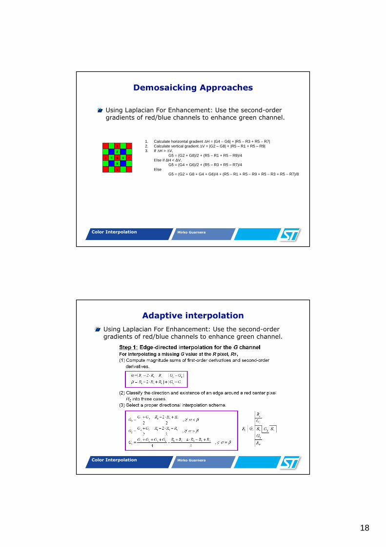
Demosaicking Approaches
Using Laplacian For Enhancement: Use the second-order gradients of red/blue channels to enhance green channel.
1
2
4 5 6 7
8
9
3
1. Calculate horizontal gradient ∆H = |G4 – G6| + |R5 – R3 + R5 – R7| 2. Calculate vertical gradient ∆V = |G2 – G8| + |R5 – R1 + R5 – R9| 3. If ∆H > ∆V,
G5 = (G2 + G8)/2 + (R5 – R1 + R5 – R9)/4Else if ∆H < ∆V,
G5 = (G4 + G6)/2 + (R5 – R3 + R5 – R7)/4 Else
G5 = (G2 + G8 + G4 + G6)/4 + (R5 – R1 + R5 – R9 + R5 – R3 + R5 – R7)/8
Color Interpolation Mirko Guarnera
Adaptive interpolation
Using Laplacian For Enhancement: Use the second-order gradients of red/blue channels to enhance green channel.
19
Color Interpolation Mirko Guarnera
Adaptive interpolation
Color Interpolation Mirko Guarnera
Demosaicking Approaches
Constant-Hue-Based Interpolation: Hue does not change abruptly within a small neighborhood.
Interpolate green channel first.
Interpolate hue (defined as either color differences or color ratios).
Estimate the missing (red/blue) from the interpolated hue.
Red Interpolated Red
InterpolateGreen
Interpolate
20
Color Interpolation Mirko Guarnera
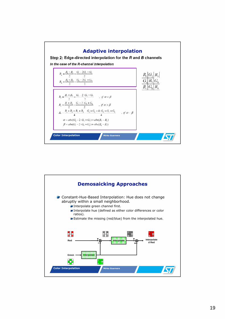
Constant Hue
we define blue "hue value" as : B/G. red "hue value" can be analogously defined. Considering the interpolation of blue pixel values : there are three different cases of blue pixel value interpolations.
Color Interpolation Mirko Guarnera
Vector SM
21
Color Interpolation Mirko Guarnera
Directional filtering
The idea behind…
Color Interpolation Mirko Guarnera
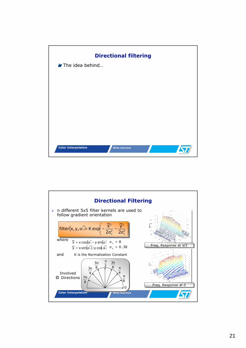
where
and K is the Normalization Constant
Directional Filtering
� n different 5x5 filter kernels are used to follow gradient orientation
( )
σ−
σ−=α
2
y
2
2
x
2
2
y~
2
x~
expK,y,xfilter
38.0
8
y
x
=σ=σ
2
π
8
π4
π8
3π
0
8
5π
4
3π
8
7π
( ) ( )( ) ( )α+α=
α−α=
cosysinxy~
sinycosxx~
InvolvedDirections
Freq. Response at π/2Freq. Response at π/2
Freq. Response at 0Freq. Response at 0
α
22
Color Interpolation Mirko Guarnera
DF
inputinput max dilatationmax dilatation
mode dilatationmode dilatation
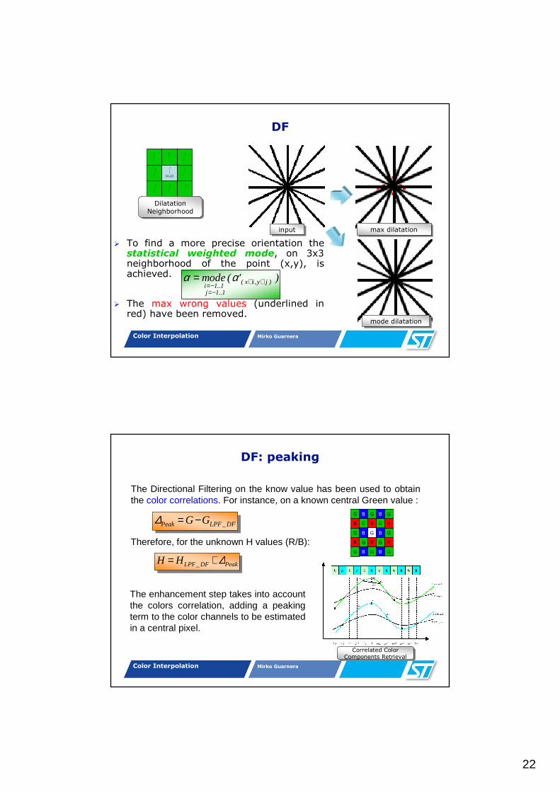
� To find a more precise orientation the statistical weighted mode, on 3x3 neighborhood of the point (x,y), is achieved.
� The max wrong values (underlined in red) have been removed.
(x,y)
DilatationNeighborhood
DilatationNeighborhood
)'( odem )jy,ix(
1..1j1..1i
++−=−=
= αα
Color Interpolation Mirko Guarnera
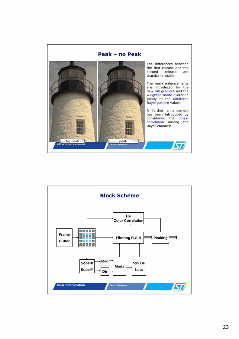
DF: peaking
The enhancement step takes into account the colors correlation, adding a peaking term to the color channels to be estimated in a central pixel.
DF_LPFPeak GG−=∆
PeakDF_LPFHH ∆+=
The Directional Filtering on the know value has been used to obtain the color correlations. For instance, on a known central Green value :
Therefore, for the unknown H values (R/B):
G
G
R
GB
RG
GB
RG
G
R
GB
RG
GB
R
G GB GB
Correlated Color Components Retrieval
Correlated Color Components Retrieval
23
Color Interpolation Mirko Guarnera
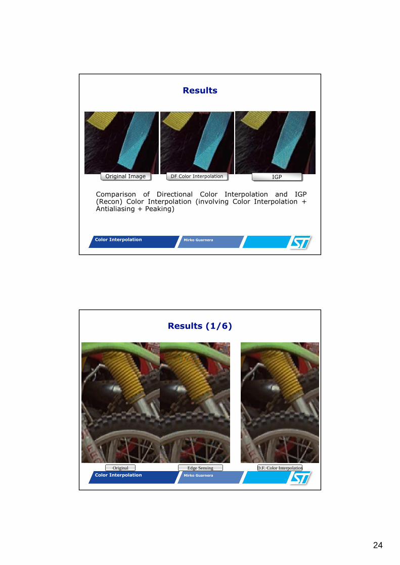
Peak – no Peak
The differences between the first release and the second release are drastically visible.
The main enhancements are introduced by the new full gradient and the weighted mode dilatation jointly to the unfiltered Bayer pattern values.
A further enhancement has been introduced by considering the cross-correlation among the Bayer channels.
No peakNo peak peakpeak
Color Interpolation Mirko Guarnera
Block Scheme
Frame
BufferFiltering R,G,B
SobelX
SobelY
Mag
DirModa
HFColor Correlation
5x5 DF
Luts
Peaking
24
Color Interpolation Mirko Guarnera
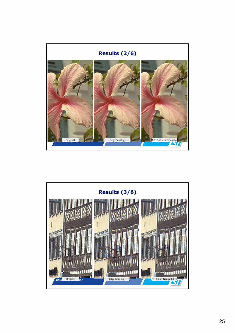
Results
Comparison of Directional Color Interpolation and IGP (Recon) Color Interpolation (involving Color Interpolation + Antialiasing + Peaking)
Original ImageOriginal Image DF Color InterpolationDF Color Interpolation IGP IGP
Color Interpolation Mirko Guarnera
Results (1/6)
D.F. Color InterpolationOriginal Edge Sensing
25
Color Interpolation Mirko Guarnera
Results (2/6)
D.F. Color InterpolationOriginal Edge Sensing
Color Interpolation Mirko Guarnera
Results (3/6)
D.F. Color InterpolationOriginal Edge Sensing
26
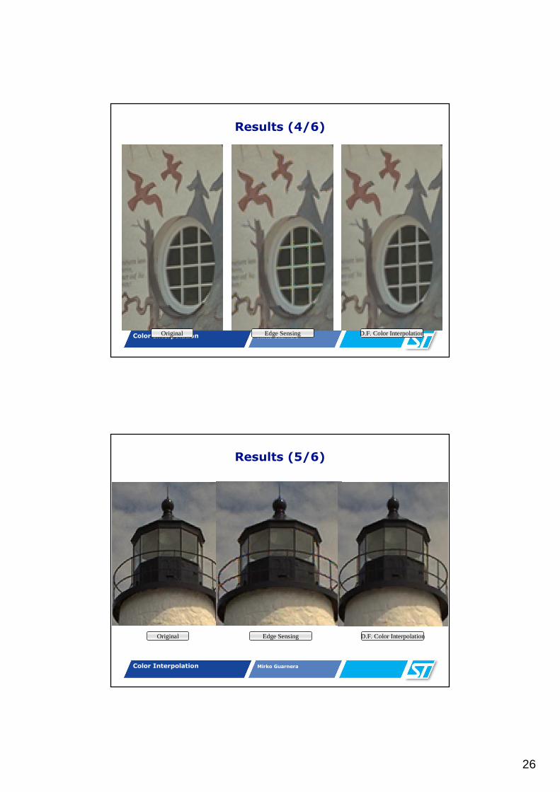
Color Interpolation Mirko Guarnera
Results (4/6)
D.F. Color InterpolationOriginal Edge Sensing
Color Interpolation Mirko Guarnera
Results (5/6)
D.F. Color InterpolationOriginal Edge Sensing
27
Color Interpolation Mirko Guarnera
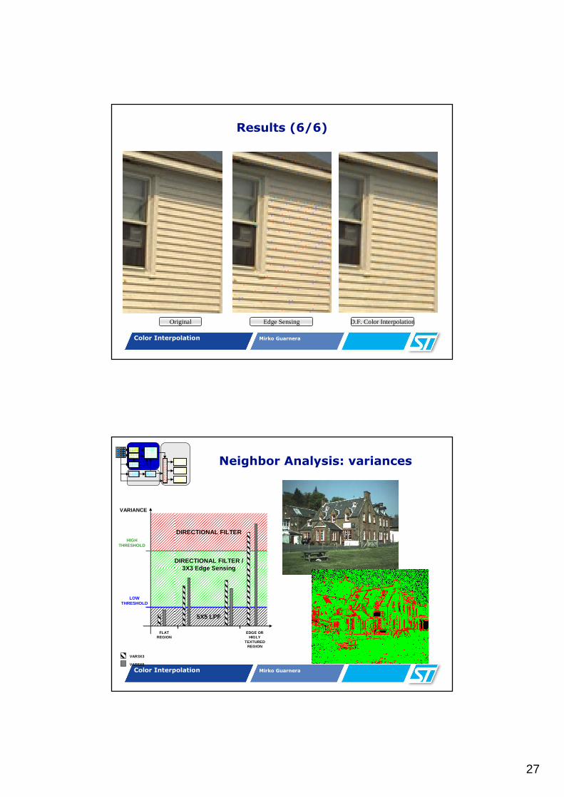
Results (6/6)
D.F. Color InterpolationOriginal Edge Sensing
Color Interpolation Mirko Guarnera
Neighbor Analysis: variances
DIRECTIONAL FILTER /3X3 Edge Sensing
DIRECTIONAL FILTER
5X5 LPF
HIGH THRESHOLD
LOW THRESHOLD
VARIANCE
VAR3X3
VAR5X5
FLAT REGION
EDGE OR HIGLY
TEXTURED REGION
28
Color Interpolation Mirko Guarnera
Color-processing sideshows
Aliasing
Resolution of sensor < spatial frequency of scene
False color
Aliasing occurs only in one or two of the color planes
Moire patterns
Overlapped patterns with near frequency
Color Interpolation Mirko Guarnera
Post processing
29
Color Interpolation Mirko Guarnera
Post processing
Color Interpolation Mirko Guarnera
Aliasing
30
Color Interpolation Mirko Guarnera
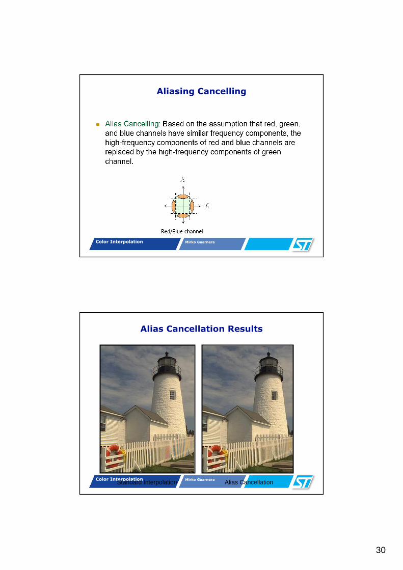
Aliasing Cancelling
Color Interpolation Mirko Guarnera Alias Cancellation
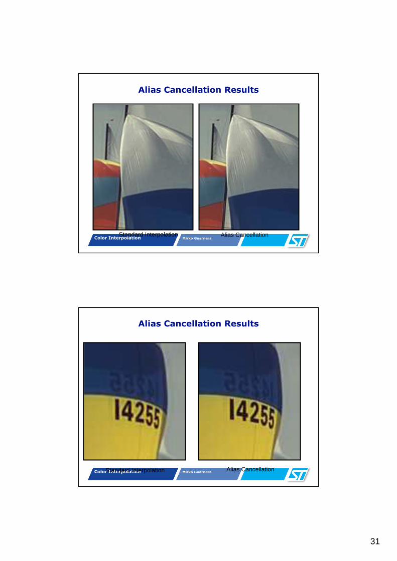
Alias Cancellation Results
Standard Interpolation
31
Color Interpolation Mirko Guarnera
Alias Cancellation Results
Alias CancellationStandard Interpolation
Color Interpolation Mirko Guarnera
Alias Cancellation Results
Alias CancellationStandard Interpolation
32
Color Interpolation Mirko Guarnera
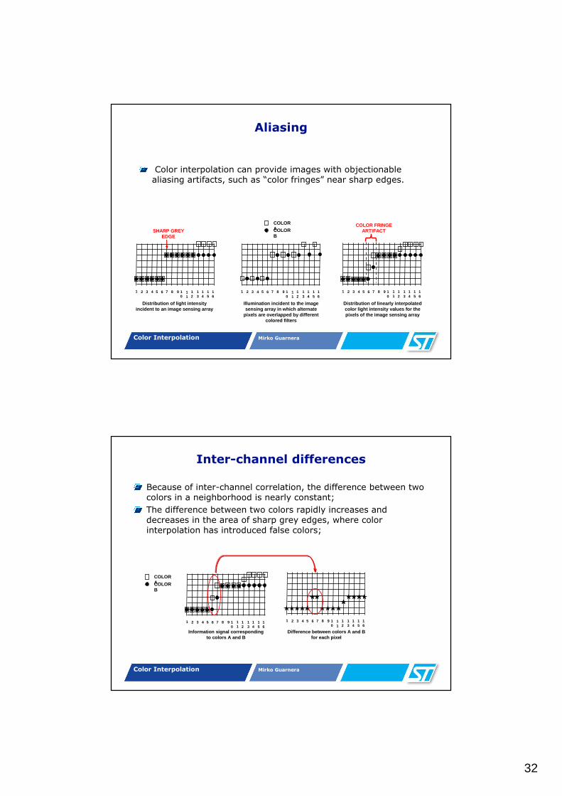
Aliasing
Color interpolation can provide images with objectionable aliasing artifacts, such as “color fringes” near sharp edges.
COLOR ACOLOR B
1 2 3 4 5 6 7 8 9 10
11
12
13
14
15
16
SHARP GREY EDGE
1 2 3 4 5 6 7 8 9 10
11
12
13
14
15
16
1 2 3 4 5 6 7 8 9 10
11
12
13
14
15
16
COLOR FRINGE ARTIFACT
Distribution of light intensity incident to an image sensing array
Illumination incident to the image sensing array in which alternate
pixels are overlapped by different colored filters
Distribution of linearly interpolated color light intensity values for the pixels of the image sensing array
Color Interpolation Mirko Guarnera
Inter-channel differences
Because of inter-channel correlation, the difference between two colors in a neighborhood is nearly constant;
The difference between two colors rapidly increases and decreases in the area of sharp grey edges, where color interpolation has introduced false colors;
COLOR ACOLOR B
1 2 3 4 5 6 7 8 9 10
11
12
13
14
15
16
Information signal corresponding to colors A and B
1 2 3 4 5 6 7 8 9 10
11
12
13
14
15
16
Difference between colors A and B for each pixel
33
Color Interpolation Mirko Guarnera
Median filter
Median filter, over a given support (e.g. 3x3 mask), operates to remove sharp spikes and valleys, leaving sharp monotonically increasing or decreasing edges intact;
1 2 3 4 5 6 7 8 9 10
11
12
13
14
15
16
Color A minus color B, median filtered with a support of 5 pixels
( ){ }( ){ }
filtermediantheofsupporttheiswhere
,|
,|
ℜ
ℜ∈−=
ℜ∈−=
jiGBmedianv
jiGRmedianv
ijijBG
ijijRG
SHARP SPIKE
REMOVED
Color Interpolation Mirko Guarnera
Color reconstruction with anti-aliasing
The median values are appropriately subtracted or added to the color received by each pixel to obtain the other two:
BGCENTERCENTER
RGCENTERCENTER
BayerCENTER
vGB
vGR
GG
+=
+=
=
ˆˆ
ˆˆ
ˆ
BGRGCENTERCENTER
RGCENTERCENTER
BayerCENTER
vvRB
vRG
RR
+−=
−=
=
ˆˆ
ˆˆ
ˆ
RGBGCENTERCENTER
BGCENTERCENTER
BayerCENTER
vvBR
vBG
BB
+−=
−=
=
ˆˆ
ˆˆ
ˆ
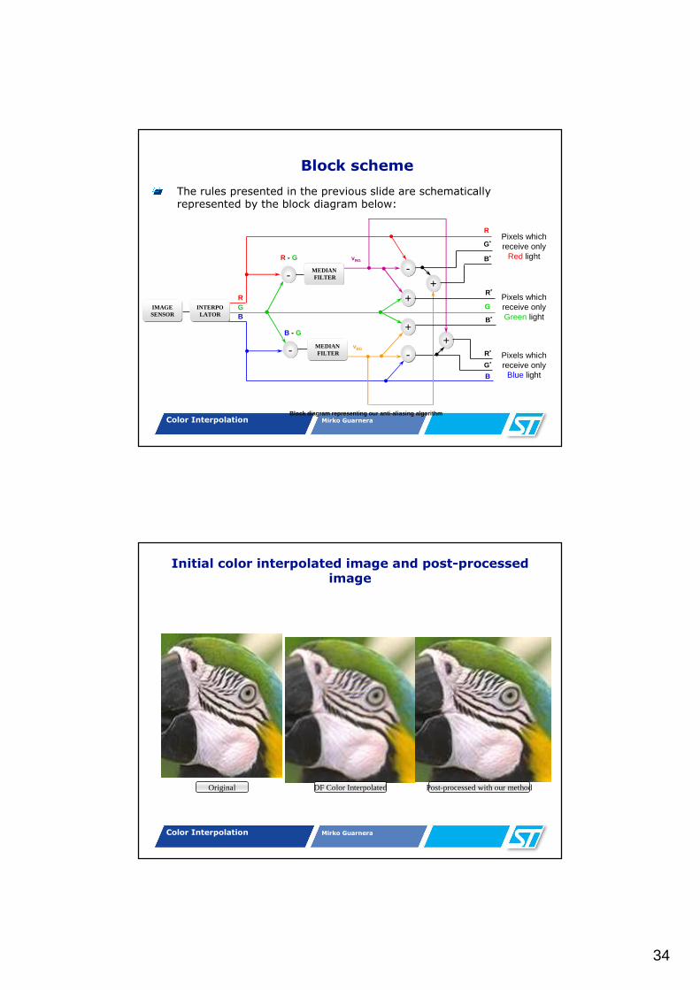
� Pixels which receive only Redlight:
� Pixels which receive only Green light:
� Pixels which receive only Bluelight:
34
Color Interpolation Mirko Guarnera
-
-
-
-
+
+
+
+
vRG
vBG
RGB
R - G
R
G*
B*
R*
G
B*
R*
G*
B
B - G
Pixels which receive only
Red light
Pixels which receive only Green light
Pixels which receive only
Blue light
MEDIANFILTER
MEDIANFILTER
INTERPOLATOR
IMAGESENSOR
The rules presented in the previous slide are schematically represented by the block diagram below:
Block diagram representing our anti-aliasing algorithm
Block scheme
Color Interpolation Mirko Guarnera
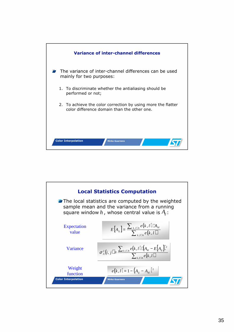
Initial color interpolated image and post-processed image
Original DF Color Interpolated Post-processed with our method
35
Color Interpolation Mirko Guarnera
Variance of inter-channel differences
The variance of inter-channel differences can be used mainly for two purposes:
1. To discriminate whether the antialiasing should be performed or not;
2. To achieve the color correction by using more the flatter color difference domain than the other one.
Color Interpolation Mirko Guarnera
Local Statistics Computation
The local statistics are computed by the weighted sample mean and the variance from a running square window , whose central value is :h
[ ] ( )( )∑
∑∈
∈⋅
=hlk
hlk kl
ij lke
AlkeAE
,
,
,
,
( )( ) [ ]( )
( )∑∑
∈
∈−⋅
=hlk
hlk ijkl
A lke
AEAlkeji
,
,
2
2
,
,,σ
( ) ( )21, klij AAlke −−=
ijA
Expectation value
Variance
Weight function
36
Color Interpolation Mirko Guarnera
In the color difference domain, a flat color differenceneighborhood is characterized by:
1. Expectation value close to the central value
2. Low Variance value
Flat color differences region
[ ] ( )[ ] ( ) oldMeanThreshBGBGE
oldMeanThreshRGRGE
ijijijij
ijijijij
<−−−
<−−−
( )( )( )( ) resholdVarianceThji
resholdVarianceThji
BG
RG
<
<
−
−
,
,2
2
σ
σ
Color Interpolation Mirko Guarnera
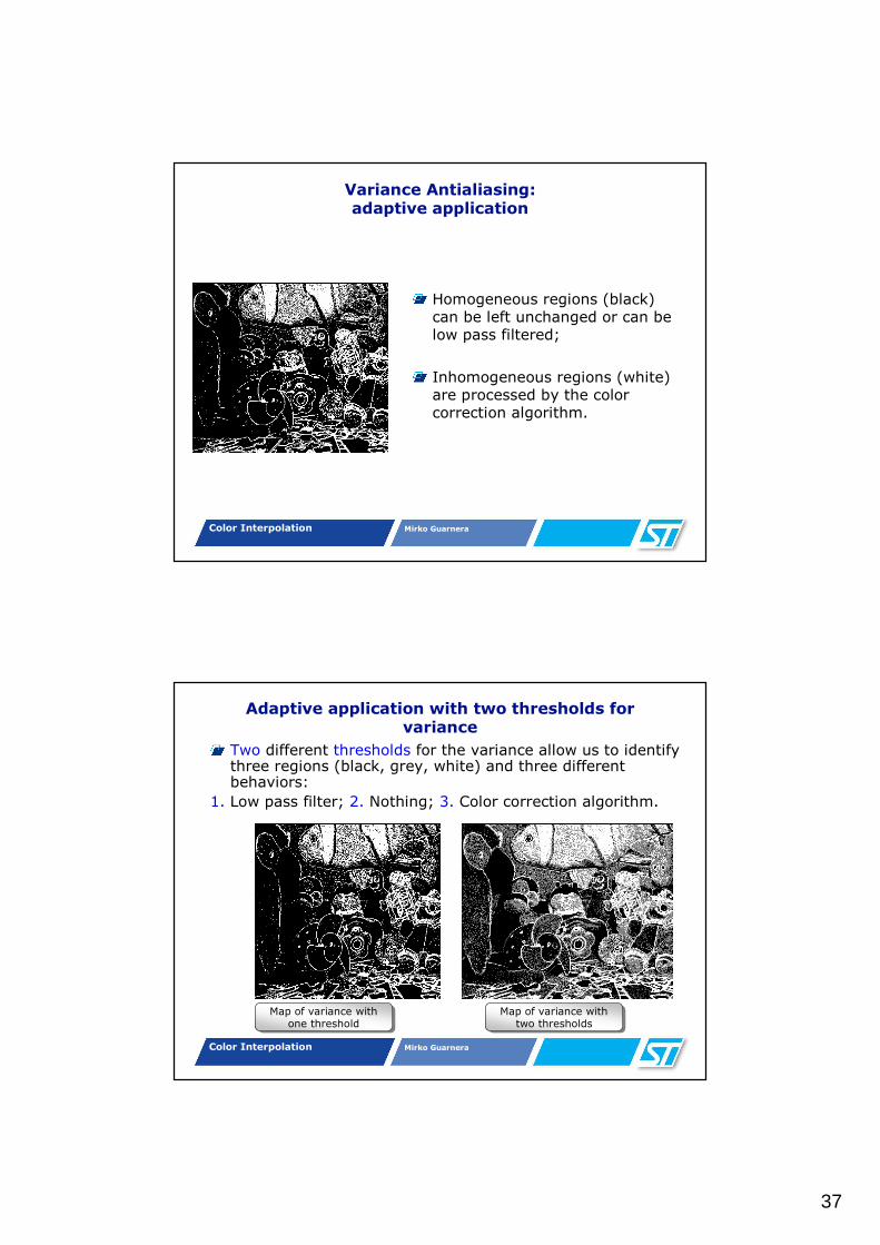
Homogeneous vs Inhomogeneous regions
According to the Expectation value and to the Variance, a map of homogeneous (black) vs. inhomogeneous (white) regions can be achieved
Processed imageProcessed image Map of homogeneous vs. inhomogeneous regions
Map of homogeneous vs. inhomogeneous regions
37
Color Interpolation Mirko Guarnera
Variance Antialiasing:adaptive application
Homogeneous regions (black) can be left unchanged or can be low pass filtered;
Inhomogeneous regions (white) are processed by the color correction algorithm.
Color Interpolation Mirko Guarnera
Adaptive application with two thresholds for variance
Two different thresholds for the variance allow us to identify three regions (black, grey, white) and three different behaviors:
1. Low pass filter; 2. Nothing; 3. Color correction algorithm.
Map of variance with one threshold
Map of variance with one threshold
Map of variance with two thresholds
Map of variance with two thresholds
38
Color Interpolation Mirko Guarnera
First Step: Two updated values for the green channel are calculated using each color difference domain:
Where
is the support of the 3x3 local windows
Variance Antialiasing:Color Correction algorithm (1/3)
GBijBij
GRijRij
BG
RG
ν
ν
+=
+=
( ){ }( ){ }hlkBGmedian
hlkRGmedian
klklGB
klklGR
∈−=
∈−=
,
,
νν
h
Color Interpolation Mirko Guarnera
Second Step: The updated value is determined by the weighted sum of the two updated values, computed in the first step, and the initially interpolated value .
The weight a is expressed as:
Variance Antialiasing:Color Correction algorithm (2/3)
Variance Antialiasing:Color Correction algorithm (2/3)
( ) ( ){ }Bij
Rijijij GaGaGG ⋅+⋅−⋅+⋅−= 11ˆ ββ
ijG
ijG
( )
( ) ( )10,
22
2
<<+
=−−
− aaBGRG
RG
σσσ
39
Color Interpolation Mirko Guarnera
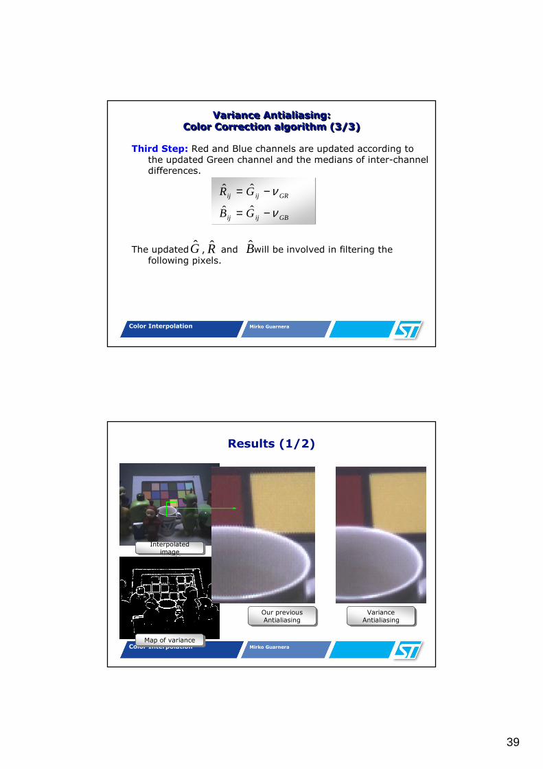
Third Step: Red and Blue channels are updated according to the updated Green channel and the medians of inter-channel differences.
The updated , and will be involved in filtering the following pixels.
Variance Antialiasing:Color Correction algorithm (3/3)
Variance Antialiasing:Color Correction algorithm (3/3)
GBijij
GRijij
GB
GR
ν
ν
−=
−=ˆˆ
ˆˆ
BG R
Color Interpolation Mirko Guarnera
Results (1/2)
Interpolated image
Interpolated image
Map of varianceMap of variance
Variance Antialiasing
Variance Antialiasing
Our previous Antialiasing
Our previous Antialiasing
40
Color Interpolation Mirko Guarnera
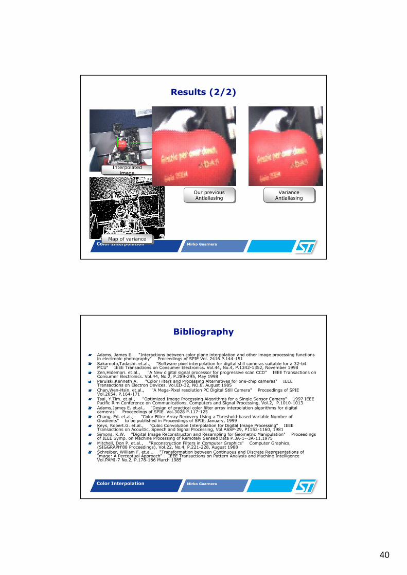
Results (2/2)
Interpolated image
Interpolated image
Map of varianceMap of variance
Variance Antialiasing
Variance Antialiasing
Our previous Antialiasing
Our previous Antialiasing
Color Interpolation Mirko Guarnera
Bibliography
Adams, James E. "Interactions between color plane interpolation and other image processing functions in electronic photography" Proceedings of SPIE Vol. 2416 P.144-151 Sakamoto,Tadashi. et.al., "Software pixel interpolation for digital still cameras suitable for a 32-bit MCU" IEEE Transactions on Consumer Electronics. Vol.44, No.4, P.1342-1352, November 1998 Zen,Hidemori. et.al., "A New digital signal processor for progressive scan CCD" IEEE Transactions on Consumer Electronics. Vol.44, No.2, P.289-295, May 1998 Parulski,Kenneth A. "Color Filters and Processing Alternatives for one-chip cameras" IEEE Transactions on Electron Devices. Vol.ED-32, NO.8, August 1985 Chan,Wen-Hsin. et.al., "A Mega-Pixel resolution PC Digital Still Camera" Proceedings of SPIE Vol.2654. P.164-171 Tsai, Y.Tim. et.al., "Optimized Image Processing Algorithms for a Single Sensor Camera" 1997 IEEE Pacific Rim Conference on Communications, Computers and Signal Processing, Vol.2, P.1010-1013 Adams,James E. et.al., "Design of practical color filter array interpolation algorithms for digital cameras" Proceedings of SPIE Vol.3028 P.117-125 Chang, Ed. et.al., "Color Filter Array Recovery Using a Threshold-based Variable Number of Gradients" to be published in Proceedings of SPIE, January, 1999 Keys, Robert.G. et.al., "Cubic Convolution Interpolation for Digital Image Processing" IEEE Transactions on Acoustic, Speech and Signal Processing, Vol ASSP-29, P1153-1160, 1981 Simons, K.W. "Digital Image Reconstructon and Resampling for Geometric Manipulation" Proceedings of IEEE Symp. on Machine Processing of Remotely Sensed Data P.3A-1--3A-11,1975 Mitchell, Don P. et.al., "Reconstruction Filters in Computer Graphics" Computer Graphics, (SIGGRAPH'88 Proceedings), Vol.22, No.4, P.221-228, August 1988 Schreiber, William F. et.al., "Transformation between Continuous and Discrete Representations of Image: A Perceptual Approach" IEEE Transactions on Pattern Analysis and Machine Intelligence Vol.PAMI-7 No.2, P.178-186 March 1985
41
Color Interpolation Mirko Guarnera
Quality evaluation
Color Interpolation Mirko Guarnera
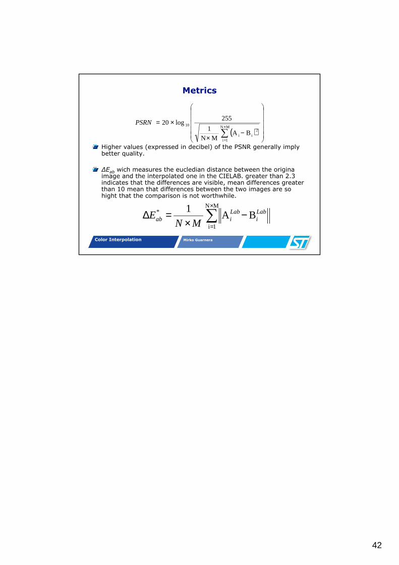
Metrics
42
Color Interpolation Mirko Guarnera
Metrics
Higher values (expressed in decibel) of the PSNR generally implybetter quality.
∆Eabwich measures the eucledian distance between the origina
image and the interpolated one in the CIELAB. greater than 2.3 indicates that the differences are visible, mean differences greater than 10 mean that differences between the two images are so hight that the comparison is not worthwhile.
( )
−×
×=
∑×
=
MN
1i
2ii
10
BAMN
1
255log20PSRN
∑×
=
−×
=∆MN
1i
* BA1 Lab
iLabiab MN
E

![New Iterative Methods for Interpolation, Numerical ... · and Aitken’s iterated interpolation formulas[11,12] are the most popular interpolation formulas for polynomial interpolation](https://img.pdfslide.us/doc/110x75/5ebfad147f604608c01bd287/new-iterative-methods-for-interpolation-numerical-and-aitkenas-iterated-interpolation.jpg)