Computer Aided Engineering and OPTISHAPE

1

The University of Michigan

Computational Mechanics Laboratory

Computer Aided Engineeringand

OPTISHAPE

Noboru Kikuchi (U of Mich)

Young Joon Song (IAE)

Seungjae Min (U of Tokyo)

Quint Corporation

2



Concept of CAE

1. What is CAE ?

2. General Concept of CAE

and Design Optimization

3. FE Analysis

3



1. What is CAE ?

• CAE stands Computer Aided Engineering

• The concept of CAE was introduced by Dr.Jasen Lemon in 1980– a professor of University of Cincinnati,

– a founder of SDRC

– a developer of I-DEAS

• CAD+FE Modeling+FEA+Design

• Utility of the Graphic Display System

4



CAD CAM

CAE

Geometric Modeling

Stress, Motion, and Flow Analyses (FEA/Mutibody Dynamics/FDA)

componentsassembly & manualcomponent tablesupplying

Process DesignOperating Design NC Tape/DataManufacturing NC Processes AssemblingEvaluation

5



Toward CIM in 1990s

• 1960s / Batch Drafting System (Plotter)

• 1960s / NC• APT(Automatically Programmed Tooling)

Language

• NC Table

• 1970s / Interactive System• Interactive CAD and Graphic NC

• 1980s / CADCAM Systems• Database and 3D Data

6



CAD in Automotive

• 1950s / General Motors• using Graphic Display System

• DAC-1 for prototype of a CAD system

• INCA for NC processing for Master Model

• CADANCE(70s), CGS(80s) + commercial soft

• 1970s and 80s / in-house CAD System• Nissan / CAD-I, CAD-II & GNC / Matuda

• Integrated CAD/CAM / Toyota

• 1990s / Commercial CAD Soft

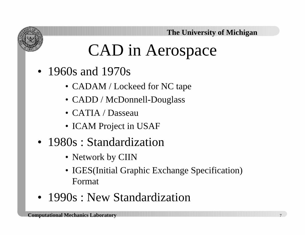
7



CAD in Aerospace• 1960s and 1970s

• CADAM / Lockeed for NC tape

• CADD / McDonnell-Douglass

• CATIA / Dasseau

• ICAM Project in USAF

• 1980s : Standardization• Network by CIIN

• IGES(Initial Graphic Exchange Specification)Format

• 1990s : New Standardization

8



CAE Concept in CAD

• CAD was originally for Computer AidedDrafting, but in 1980s CAD becomes morefor Computer Aided Design based on

• wire frame models

• surface models

• three-dimensional solid models

• More toward Design Analysis andEvaluation by FEA

9



CAE concept in CAM

• CAM is Computer Aided Manufacturingmostly for automated process control of NCmachines, but

• Computer Simulation for Process Designand Process Control becomes important incomputer aided manufacturing in 1980s

• Sheet Metal Forming, Forging, Molding,Die Design based on Computer Simulation

10



CAE in 1980s & 90s

• Design Analysis and Evaluation by FEA• Linear and Nonlinear Structures

• Temperature, Magnetic Fields

• Fluid Flows ( Mostly by FDA & FVA )

• Process Simulation• Kinematics, Rigid Body Dynamics, Multi-Body

Dynamics for Assembly Lines, Robots, ..... byADAMS, DADS, and others

• Forming Process Simulation by Explicit FEA

11



Lots of Sophisticationand

Great Success

Realization of importance andprofitability of Geometry Based

CAD/CAM and CAE

12



Market of CAD/CAE

MSC/ Dr. McNeal

CAD

Vendors

CAD

Revenue

CAE

Vendors

CAE Revenue

COMPUTERVISION 260 MSC 80

CATIA (IBM) 206 PDA 38

PARAMETRIC 167 SWANSON 32

UNIGRAPHICS (EDS) 165 RASNA 17

SDRC 157 HKS 12

AUTODESK 143 MARC 11

OTHERS 199 OTHERS 143

13



Trend In MCAE

l CAE is now widely accepted– 1980 J. Lemon / SDRC– integration with CAD

l RASNA-MECHANICA and PRO-E / I-DEAS Master

– Design Optimizationl Size/Shape/Topology Optimization

l Automatic Mesh Generation for FEAl Modeling Probleml Further development is demanded

14



Cost Reduction• CAD shows quite the success to make

change of engineering, but CAE is stillregarded to be expensive, because– Modeling is time consuming

– Analysis results are difficult to be reflected todesign change

– Analysis is limited to Safety/Liability Study

– Few experts of software

• Link with CAD & CAE is seeking

15



2. General Concept of CAE

• CAE (Computer Aided Engineering) shouldnot be just for computer aided engineeringanalysis

• CAE should have large extent of• Design Analysis and Evaluation

• Re-Design and Design Optimization

• Process Simulation

• CAE is the connector of CAD and CAM

16



Two Kind of CAE

• MCAE (Mechanical CAE)– Structures (Linear and Nonlinear)

– Explicit FEA (Forming, Crash, ..., Simulation)

– Multi-Body Dynamics (Simulation)

• FCAE (Fluid CAE)– Heat Transfer/Conduction

– Newtonian and Non-Newtonian Fluid Flow

– Mold Flow Simulation

17



MCAE and FCAE

• Two separate CAE groups with twodifferent pre/post processors as well asanalysis soft– expensive, time consuming, disjointed

communication, and difficult management

• CIM requires integrated coupled designstudy of MCAE and FCAE

18



Three Types of CAE

l Stand Alone CAE– standard FEA based CAE codes– special analysts oriented high accuracy– independent CAD and Pre-Processing

l CAD Linked CAE– present trend / link with CAD– automatic mesh generation methods

l CAD Imbedded CAE - Design Oriented

19



Market Change in MCAE

Dr. McNeal at MSC

1995 1999

CAD Independent

CAD Linked

CAD Imbedded

Total

CAE

225 M$ 175 M$

100 M$ 300 M$

75 M$ 400 M$

875 M$400 M$

20



CAD Imbedded MCAE

l CAD side takes leadershipl Simulation of design feasibility

– users are designers rather than analysts

– less accuracy but user oriented

– CAD/CAE link must be completed

– CAE is an icon of CAD menu

l Short Turn Around Time

DESIGN ORIENTED

21



Present Demandl For Shortening of Turn Around Time by

Simplifying FE Modeling Methods– CAD Linked Automatic Mesh Generation– Adaptive FE Methods (h and p elements)

– Meshless FE Methods (ANALYSIS)

l Integration for Production Engineering– Modeling, Analysis, Design, Manufacturing– Paradigm change may be required

22



Five Step CAE Procedure

Modeling

FE Analysis and Simulation

Re-DesignDesign Optimization

Rapid Prototype

Test/Evaluation

23



Design Optimization

• has been considered mostly in structuresunder linear elasticity–

– STRUCTURAL OPTIMIZATION

• recently it is extend to Mechanical Designin more general sense

• few work on heat, fluid flow, multi-bodies

24



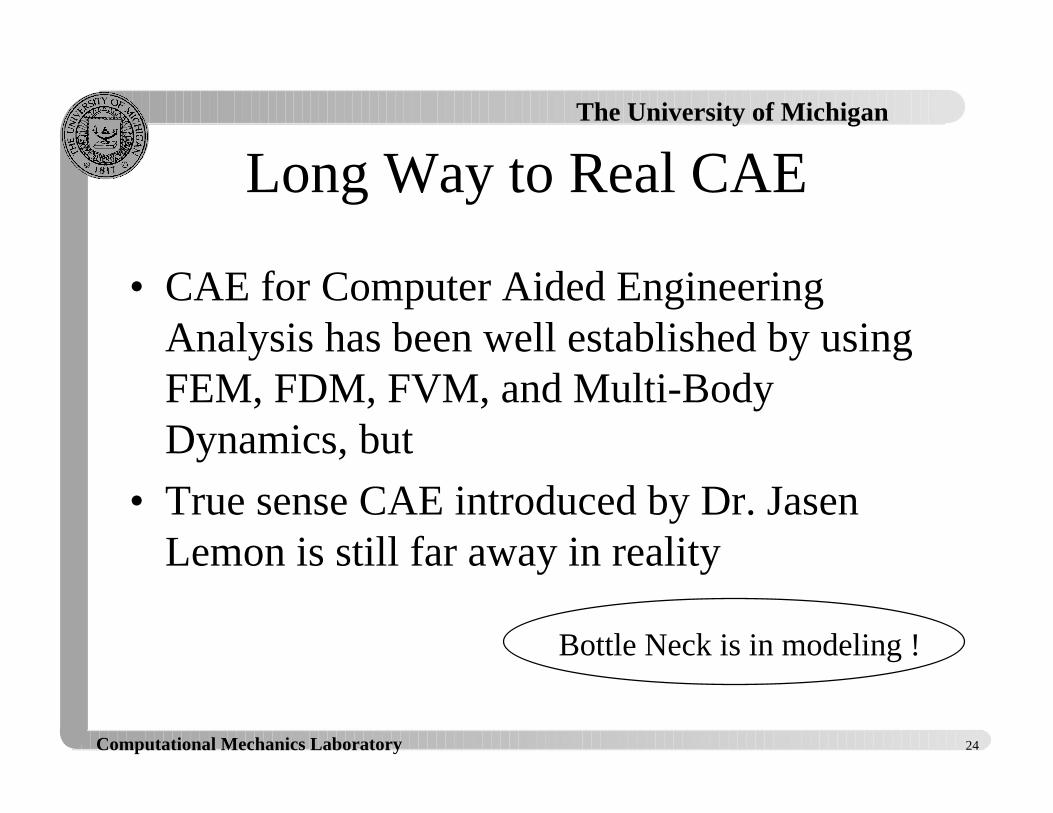
Long Way to Real CAE

• CAE for Computer Aided EngineeringAnalysis has been well established by usingFEM, FDM, FVM, and Multi-BodyDynamics, but

• True sense CAE introduced by Dr. JasenLemon is still far away in reality

Bottle Neck is in modeling !

25



Key Components of CAE

• Modeling / 70%– Link with CAD Data

– Automatic Mesh Generation Methods

– Input of Load/Support Condition

• FEA (Finite Element Analysis) / 10%

• FES (Finite Element Simulation) / 10%

• Redesign & Optimization / 20%

26



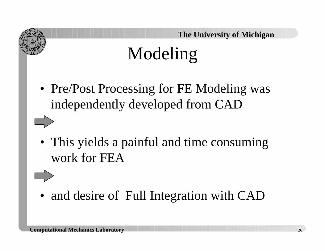
Modeling

• Pre/Post Processing for FE Modeling wasindependently developed from CAD

• This yields a painful and time consumingwork for FEA

• and desire of Full Integration with CAD

27



Link with CAD in Modeling

• Link is already exists in– SDRC I-DEAS Master Series

– PRO-E and RASNA-MECHANICA

• Link must be established for most of FEA,especially for Pre/Post Software for FEA– MSC/PATRAN ----- UNIGRAPHICS (?)

– HYPERMESH ----- ????

– Others

28



Link with CAD

• leads paradigm change in CAD and CAEpractice in industry and in education, too

• CAD soft is absorbing CAE, especially,CAD soft must be linked with FEA Pre/Postsoft for full integration

• CAD side must take leadership to do so, inorder to make real CAD not for drafting

• This movement has already started .....

29



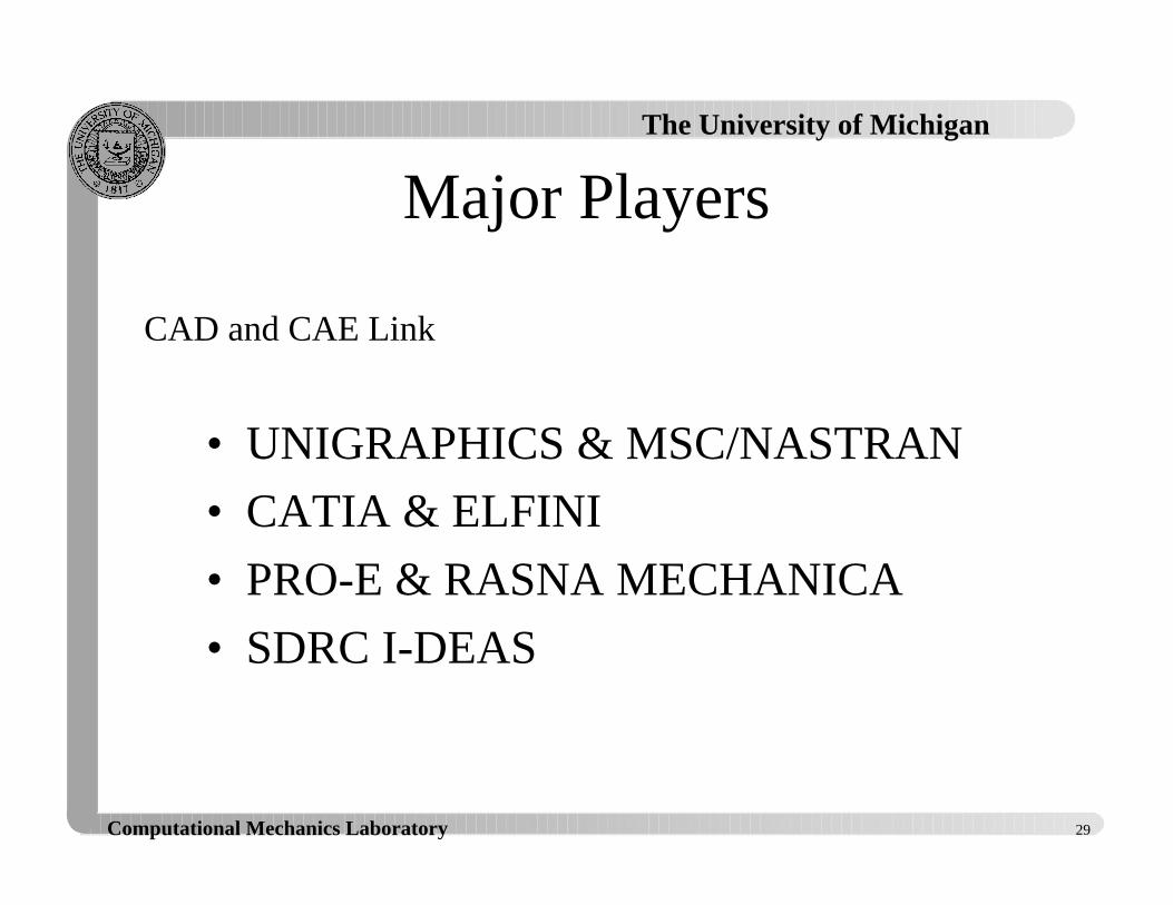
Major Players

• UNIGRAPHICS & MSC/NASTRAN

• CATIA & ELFINI

• PRO-E & RASNA MECHANICA

• SDRC I-DEAS

CAD and CAE Link

30



Modeling & Design

• Choice of design variable linked with CAD– circle and arc (radius,angle, center location)

– ellipse

– control points of Bezier, B-, and NURBS• three modules ( CAD modeling, Automatic Mesh

Generation, and Design Modification ) must beintegrated ...... very difficult task

• most of structural optimization software developedin 1970s took this approach .... ELFINI, SAMSEF

31



Bezier & B-Spline

• Bezier Surfaces– P.de Casteljau at Citroen (no publication)

– P. Bezier at Renaut

– 1974 conference at the university of Utah

• B-Spline Method– Bezier Surfaces + Coons Patch

• NURBS (Non-Uniform Rational B-Spline)

32



Difficulty

• For shape design optimization, link withCAD system seems to be the most effective,if FE modeling ( especially mesh generation) is fully imbedded in the whole system.– No CAD system fully support design

optimization and FEA, except SDRC/I-DEAS

– CAD-like Preprocessor for FEA can be utilizedfor shape design optimization, but it isdisjointed with standard CAD systems

33



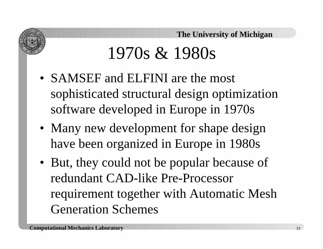
1970s & 1980s• SAMSEF and ELFINI are the most

sophisticated structural design optimizationsoftware developed in Europe in 1970s

• Many new development for shape designhave been organized in Europe in 1980s

• But, they could not be popular because ofredundant CAD-like Pre-Processorrequirement together with Automatic MeshGeneration Schemes

34



Paradigm Change

35



Design Optimization

• Design Variables should not be linked withCAD data– Sizing Optimization

– restrict to beam/frame-like structures

– Shape Optimization– GENESYS Approach is most likely choice

– Topology Optimization– density or homogenization design approach

36



GENESYS Approach

• Design change is considered to be a linearcombination of basis design shapes

d dk kk

m

==

∑α1

d kk

k

==

th pattern of design

design variableα

37



Characteristics

• FE Meshes are subordinated to the baseshape design so that automatic remeshingmethods need not be integrated into thedesign optimization system, but

• This may lead excessive mesh distortionduring the design process, and then someautomatic distortion correction scheme isdesirable

CAD independent

38



Density and Homogenization

Gray Scale = Density

d kk = density of th pixel / voxel

dk =RS|T|

1

0

if occupied by solid structure

if structure is perforated

if no structure is placed

α

Shape is recognized by a set of on pixels

39



Characteristics

• Design optimization is completelydecoupled with any sort of mesh adaptation

• Shape and topology design variables aretransformed into the density of material orelasticity matrix of material which isassigned in each finite element of a fixedFE model, at least a fixed FE meshgenerated at the initial time.

40



This approach leads 1990s

OPTISHAPE from QUINT

OPTISTRUCT from ALTAIR

ANSYS-Topology

MSC/NASTRAN-Topology

41



Exercise #1 : OPTISHAPE

Load #1

Load #2

100 kN

50 kN

Structural Steel200 GPa0.3

0.5 m

0.3 m

thickness of a plate = 1 cm

42



Two loads are considered : Load #1 is a tensile force, andLoad #2 is a bending force. Apply OPTISHAPE with thevolume constraint (25% of the rectangular design domain)to the following three cases :

(1) Load #1 is applied at the center of right edge (2) Load #2 is applied at the center of right edge (3) Load #1 and #2 are applied at the same time (4) Load #1 and Load #2 are applied independently

Find the nature of the optimum structures to these loadingconditions. Especially, observe the difference between (3)and (4).

43



Exercise #2Fixed End

Fixed End

Load #1 10 kN/cm

Load #2

4 cm

10 cm

2 cm

thickness 2 mm

50 kN

Structural Steel

44



Two loads, a distributed edge load #1 and a point load #2are considered for a 2 mm thick L-shape folded plate asshown in the figure. Consider reinforcement of this L-shapefolded plate by adding 2 mm high ribs in the 20% of thedesign domain for the case that two loads are appliedindependently.

You may solve this by using OPTISHAPE, but if you haveother software for FE analysis and/or structural optimization,solve this by using those software, and make comparison theresults obtained by both methods.

45



Optimum Structural Designin CAE

1. CAE and Design Optimization

2. Redesign and Optimization

3. Size and Shape Design Optimization

46



CAE and Design Optimization

1. Structural Optimization

2. Typical Setting of Design Problems

3. Characteristics

4. General Remarks on Stresses

47



Structural Optimization

• A small portion of Mechanical DesignOptimization which involves mechanicalsystems, multi-body mechanisms/structures,and individual structural components

• The concept of Multi-DisciplinaryOptimization is required in mechanicalsystem design, but this is far from thereality of structural design optimization

48



Many Design Problems

• Design in Linear Elastic Structures– Global Stiffness Maximization

– Strength Maximization (Composite Laminates)

– Frequency Response Problem

– Dynamic Stiffness Maximization

– Frequency Control Problem

– Buckling Load Maximization

• Design in Nonlinear Structures & Processes

49



Mechanical Design

• Maximizing formability of sheet metals

• Minimization of holding forces of sheetmetals

• Maximization of quality of sheet forming

min ,design

pricipal strainsε ε

εε ε1 2

21 2

−=l q

mindesign

11

11 2 1 2− − − − −zε ε ε εb g b gΩ

ΩΩ

d

Very Complex !

50



Typical Setting

internal virtual work

external virtual work

l d dT

v v v bd v tT T

t

b g b g= ∂ + +z z zσ ρ0 Ω Ω ΓΩ Ω Γ

minmaxl l

a lu

u,v u vb g

b g b g≤

= ∀

Total Weight

a dT

u,v v E u v udTb g b g b g= ∂ ∂ −z zΩ ΩΩ Ω

ω ρ02

51



a dT

Elasticity Matrix Strain Vector

Shifted Excited Frequency Mass Density Displacement Vectorin Equilirium

u,v v E u

v u dT

b g b g

2

= ∂ ∂FHG

IKJ

−

zz

Ω

Ω

Ω

Ωω ρ0

2

( )

Internal Virtual Work

52



σ ε σ= −E 0

Strain-Displacement Relation

Stress-Strain Relation

ε v

v

v

v

v

v

v

ub g

b gb gb gb gb gb g

=

R

S

||||

T

||||

U

V

||||

W

||||

=

∂∂

∂∂

∂∂

∂∂

∂∂

∂∂

∂∂

∂∂

∂∂

L

N

MMMMMMMMMMMMMM

O

Q

PPPPPPPPPPPPPP

RS|T|

UV|W|

= ∂

εεεγγγ

x

y

z

yz

zx

xy

x

y

z

x

y

z

z y

z x

y x

v

v

v

0 0

0 0

0 0

0

0

0

E ==Elasticity Matrix

initial stressσ 0

53



l d

d

T

Work Done by Initial StressT

Work Done by Body Force Work Done by Traction

v v

v bd v t

E

T T

t

b g b g= ∂

+ +

zz z

=

σ

ρ

0

0

Ω

Ω Γ

Ω

∆

Ω Γ

σ α

1 244 344

1 24 34 124 34

External Virtual Work (Work potential)

l u b tb g l q= mean compliance by σ ρ0

54



Mean Compliance

If the thermal stresses, body forces, and tractions are specified,if the displacement resulted by such applied forces is small,it means that the structure is stiff in its global response.

Minimization of the Mean Compliance= Maximization of the Global Stiffness

If constrained displacement is specified on the boundary, thenthe resulted stress (that is traction) on the boundary must be large if the structure is stiff. In this case, we have to

Maximize the Mean Compliance

55



Discrete Form / FEM

K = B EB N NdTT

stiffness matrix mass matrix

dΩ ΩΩ Ωz z−

1 24 34 1 24 34ω ρ0

2

f B N bd N tT T

t

= + +z z zT d dσ ρ0 Ω Ω ΓΩ Ω Γ

Shifted Stiffness Matrix

Generalized Load Vector

minmaxu f

Ku= f

T l≤Total Weight

56



Equivalent Formulation

minKu= f

Tu f

ρd WΩΩz ≤ 0

minmaxu f

Ku= f

T ld

≤z ρ ΩΩ

They are the dual problemsand are equivalent.

Minimizing the meancompliance with thevolume constraint

Minimizing the volumewith the mean complianceconstraint

57



Compliance and Energy

Ku = f u Ku = u fT T⇒

Mean Compliance = Twice of the Total Strain Energy

u fT = work done

minv

T T Tv u u Ku u f u fI Ib g b g4= = − = −minimum potential energy

at equilibrium

1

2

1

2

58



Equivalent Formulation

min min min max mindesign design design

I Iu f v vT

v v= − = −2 2b ge j b g

Using the relation

we can define the optimum design problem by

max mindesign

Iv

vb gby using the total potential energy

59



Design Optimization

The most fundamental structural design problem can be stated as the maximization of the minimum total potentialenergy of a structural system with respect to designs andadmissible displacements

max mind v

60



Stress and Compliance

1 2 1

3

1 12 2

E ET+

≤ ≤ν

σ σ σν

σb g

C

σ σ σ σσσσ

21 2 3

1

2

3

11

2

1

21

21

1

21

2

1

21

=

− −

− −

− −

L

N

MMMMMM

O

Q

PPPPPP

RS|T|

UV|W|

l q

ε ε σ σ σ σ σ σT T T T

EE = C C=

− −− −− −

L

NMMM

O

QPPP

=1

1

1

1

ν νν νν ν

Mises Equivalent Stress

strain energy density

relation

61



Stress Singularity

Stresses become infinite as well as the strain energy density(Essential Singularity)

Stresses become infinite, but thestrain energy density is finite in the sense that it is integrable (Normal Singularity)

62



Local Stress

• Stresses can be infinite in continuumstructures ( Plates/Shells, Solids ), whilestresses are finite for trusses, beams, andframes.

• Thus, making the upper bound of the localstress value itself does not make sense.

• Some sort of integral (average) form ofstresses should be constrained.

63



Candidates

σ σ σe de

= ≤z 2

1

2ΩΩ max

Average Stress Bound in a Finite Element

The finite element model must be fixed duringthe optimization

σν

σ σ σ2 3

2 1d

Ed

e e

TΩ ΩΩ Ωz z≤

+≤b g C max

Noting that

the element strain energy can be used for stress constraint

64



Note 1

σ σT T Td de e

C E u KuΩ ΩΩ Ωz z= =ε ε

can be calculated much accurately than

σ2de

ΩΩz

since the first derivatives of the displacement must becalculated to evaluate the Mises stress

65



Note 2

• Mean compliance was introduced by Pragerand Taylor to define structural optimizationfor continuum solids and structures

• Weight minimization with stress anddisplacement constraints was introduced fortrusses, beams, and other space frame typestructures in aerospace and civil engineering

stresses are bounded in these frame structures

66



Indirect Stress Control

Compliance

Maximum Mises Stress

σmax

lmax1 lmax2 lmax3

67



Three Major Design Problems

• Sizing Optimization– thickness and cross

sectional properties

• Shape Optimization– Location of holes/arcs

– Radii of holes/arcs

– control points of splines

• Topology Optimization– number of holes

– shape of holes

Thickness

Shape of the Outer Boundary

Internal Hole 1

Hole 2

Topology = numberof holes

68




fixed end

thick hollow square barmade of structural steel

Load #1 / Bending I

Load #2 / Bending II

Load #3 / Torsion

69



Exercise #4 : A Cross Section

Design Domain of the Cross Section

3 cm

4 cm

1 cm

2 cmHole

Using 30% area of the outerrectangle, design the crosssection with a specified rectangular hole that canmaximize

1. Bending Rigidity2. Torsional Rigidityand3. Shear Rigidity

70



Exercise #5 : A JointTorsional Loading #2

Axial Loading #1

Torsional Loading #2

Bending Loading #3

Box Beam ( Thick Folded Plate & Welded )

This is a conceptual abstractfigure of a joint portion of anautomotive body structure.When the thick box beam isdesigned, state possible threedifferent structural optimizationproblems : sizing, shape, andtopology problems.

71



Assuming the rigid welding at the joints,find the optimum location (a,b) of the left webas well as the thickness of the flange and web (t1,t2).

Welding

a

b

thickness t2

thickness t1

a

b

6 cm

4 cm

upper flange

lower flange

left web right web

(fixed)(design)

Additional Design Problem

72



Simply Supported

Distributed Load20 kN/cm

20 cm

40 cm

30 cm

15 cm

5 cm

Quadratic Curve

Structural Steel2 mm thickness

Exercise # 6 : Shell

Consider a shell structurewhich has two circularholes, whose thicknessis 2mm made of steel.When it is subjected toa uniformly distributedload at the top circularedge, find the optimumreinforcement by using30% of the total area ofthe shell. Here the bottomcircular hole is simplysupported.

73



When OPTISHAPE is applied to this shell structure,reinforcement should be always placed along the top,bottom and internal hole edges with 5 mm wide.

74



Redesign and Optimization- Fully Stressed Design -

Sizing Design Optimization

Optimality Condition

Fully Stressed Design

Redesign Method

1st Generation Software

75



Sizing Optimization

• 1960s : Prof. L.Schmit’s Leadership– Mathematical Programming (Minimization)

– Finite Element (Matrix Structural ) Method

• Design Sensitivity Analysis : Fox 1967

Ku = fK

du + K

u

d

f

d⇒

∂∂

∂∂

=∂∂

∂∂

= −∂∂

+∂∂

FHG

IKJ

−u

dK

K

du

f

d1

76



Design Sensitivity

DD

g

d

g

d

g

u

u

d

g

d

g

uK

K

du

f

d=

∂∂

+∂∂

∂∂

=∂∂

+∂∂

−∂∂

+∂∂

FHG

IKJ

−1

g u,d gb g ≤ max

Performance FunctionsObjective Function & Constraints

Design Sensitivity ( Direct Method )

77



Dual Method

K H =g

uH KK =

g

uKT

n n n mm n

T

T

× ××

− −∂∂

F

HGG

I

KJJ ⇒

∂∂2 0

1 1

Defining the dual (conjugate) problem

Design sensitivity can be computed by

DD

Tg

d

g

d

g

u

u

d

g

dH

K

du

f

d=

∂∂

+∂∂

∂∂

=∂∂

+ −∂∂

+∂∂

FHG

IKJ

78



Direct & Dual Methods

• If the number of design variables is smallerthan that of design constraints, the directmethod by computingis more efficient

• On the other hand, if the number ofconstraints is much larger than that ofdesign variables, then the dual method ismuch more efficient.

∂∂

= −∂∂

+∂∂

FHG

IKJ

−u

dK

K

du

f

d1

79



Fundamental Reference

R.L. Fox, Optimization Methods forEngineering Design, Addison-

Wesley, 1971

80



In Practice

• In most of mechanical design problems, it isdifficult to express the constraints in explicitfunction forms No Analytical Sensitivity

• For example, strength of a thin walledstructural component– yield criterion for ductile materials

– maximum principal stress for brittle materials

– buckling load for compressive loading

81



Finite Difference Method

DD

g

d

g d d u d d g d u

d

g d d u d d g d d u d d

d

g d u g d d u d d

d

≈

+ + −

+ + − − −

− − −

R

S

||||

T

||||

∆ ∆

∆∆ ∆ ∆ ∆

∆∆ ∆

∆

, ,

, ,

, ,

b gc h b g

b gc h b gc h

b g b gc h2

Central difference approximation is regarded as the best methodto calculate the design sensitivity, even for shape design case.

82



Note• Mechanical design problems are

represented by rather few design variableswith a lot of design constraints– finite difference approximation

– dual method for analytical evaluation

• Aerospace and civil engineering structuraldesign, we have many design variables, andthen finite difference approach is noteffective Frames + Shear Panels

83



Exercise #7 : Sensitivity

Using the shell structure we have used in Exercise #6, find thesensitivity of the maximum Mises stress with respect to thediameter of the internal holes. Compute the design sensitivityby using the finite difference approximation.

84



Example of Design Sensitivity

for

Truss-like Structures

85



No Major Problems

min,

max

A e e ee

E

e i

A Lx

ρ=

∑1

σ σ σee

e= ≤max max

u ui ii= ≤max max∆

Weight Minimization

Subject To

(Stress Constraint)

(Displacement Constraint)

Design Variables

Cross Sectional Area & Joint Location (Size + Shape)

86



Typical Performance Functions

DDA

A L LD

DA L

LA

ee e e

e

E

e ei

e e ee

Ee

ie eρ ρ ρ ρ

= =∑ ∑

FHG

IKJ =

FHG

IKJ =

∂∂1 1

max max

&x x

Total Weight of a Truss/Frame Structure

Maximum (Axial) Stress

DDA

EL A

DD L

L EL

e

e

e

e

e

e

e

i

e

e

e

i

e

e

e

i

σ

σ σ

= −∂∂

= −∂∂

+ −∂∂

1 1

1 1

l q

l q

u

x x

u

x

87



Lagrangian

L A Le e ee

E

e e i iT

ii

n

= − − − −= =

∑ ∑ρ λ σ σ µ1 1

max

max maxb g e ju u ∆

Lagrangian

− − − −= =

∑ ∑δλ σ σ δµe ee

E

i iT

ii

n

max max

max b g e j1 1

u u ∆

First Variation

δ ρ λ µ δL LA A

Ae e ee

ei

iT

i

i

i

ei

n

ee

E

= −∂σ∂

−∂

∂∂∂

FHGG

IKJJ==

∑∑u u

u

u

11

max

88



KKT Condition

λ σ σ λ σ σe e e e− = ≤ − ≤max max, ,b g 0 0 0

µ µi iT

i i iT

iu u u u− = ≤ − ≤∆ ∆max max, ,e j 0 0 0

From the variation of the Lagrange multipliers,

This implies that if the inequality constraint is not saturated,the Lagrange multiplier must be zero. Conversely, if the Lagrange multiplier is non-zero, the constraint must be saturated.

89



Optimality Condition

λρ µ

e

e e iiT

i

i

i

ei

n

e

e

e

ee

LA

AA

A=−

∂∂

∂∂

∂σ∂

∂σ∂

≠ ∀δ=∑

u u

uu

1 0if and if

ρ ρ µ λ σ σe e e e iiT

i

i

i

ei

n

e eL LA

≠ ≠∂

∂∂∂

⇒ ≠ ⇒ − ==∑0 0 0

1

& max

u u

u

u

First Approximation : Fully Stressed Design

σ σσ

σee e E= ⇔ = =max

maxmax, ,...,1 1

90



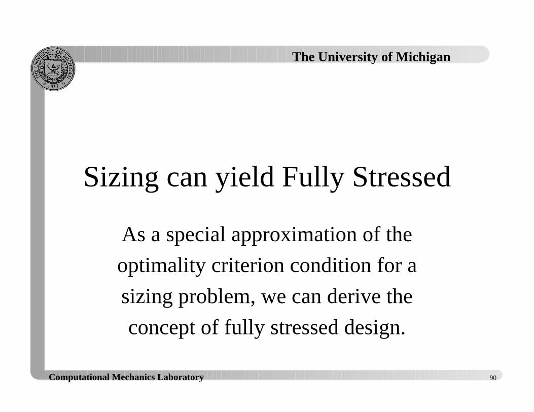
Sizing can yield Fully Stressed

As a special approximation of the

optimality criterion condition for a

sizing problem, we can derive the

concept of fully stressed design.

91



Interpretation

If the displacement constraint is not saturated at a node ofthe e-th truss member, its Lagrange multiplier must be zero.Thus, we have

λ ρe e ee

e

LA

=∂σ∂

Since the mass density and the length of the truss elementare positive, this yields

λ e ≠ 0

There fore, the constraint on the stress must be saturated.

92



Fully Stressed

Thus, if the displacement constraint is not imposed, the fullystressed state is nothing but the optimum. Therefor, even ifthe displacement constraint is imposed, in the most of trussmembers which are not related to the maximum displacementthe fully stressed condition must be satisfied, and then it canbe said that the fully stressed state must be a good approximationof the optimum state.

Many Design Codes in 1950s and 60swere made for Fully Stressed Design

L.Schimit disproved this need not be true.

93



Fully Stressed Design Method

A A kek

ek e+ =FHG

IKJ =1 1 2b g b g σ

σα

α

max

, , ,...... for some

x x x xik

ik

eik

ik e

e

i+

=

= + − −FHG

IKJ

RS|T|

UV|W|

∑1

1

1b g b g b g b ge j σσ

α

max

max

Sizing / Cross Sectional Area

Shape / Length & Nodal Coordinate

x1i

e=1

e=2

x2i

xi

94



Fully Stressed Design

• Fully stressed design was the design methodbefore mathematical programming methodwas introduced in 1960 by L. Schmit

• An effective method to find out the initialstart (initial approximation) of the MPM

• This can be a Re-Design method

• This can be extended to other physicalquantities and other type structures

95



Other Physical Quantities

• Mises equivalent stress on a boundary

• Maximum principal stress

• Maximum shear stress

• Principal Strains and/or Formed Thickness

• Strain energy density

• ................... Anything Distributed along/on

• ................... the Design Boundary/Domain

96



Fully Stresses Design

• Design variable and the quantity to besaturated must be defined in the one-to-onecorresponding way

Axial stress is not constantin each beam element, andthen the design variable Aeof the cross sectional area must be defined as the axialstress.

A x A xx hk k+ =

±FHG

IKJ

1 2b g b gb g b g b gσ

σ

,

max

97



Natural Extension

thickness h(x,y)distribution

Plate/Shell Like Structures

1) Mises Equivalent Stress

h x y h x yx y h x y hk k+ =

+ −FHG

IKJ

1 2 2b g b gb g b g b g b gm r, ,

max , , , , ,

max

σ σ

σ

α

2) Strain Energy Density

h x y h x yx y h x y h

k k

T T

+ =+ −RST

UVWF

H

GGG

I

K

JJJ1

12

212

2b g b gb g b g

b g b g, ,

max , , , , ,

max

ε ε ε εE E

σ

α

98



Elliptic Hole Design

a

b

(x0,y0)

Design variables are a,b, and x0,but the stresses are defined alongthe boundary of an elliptic hole

r x yθb g b g= radial distance from the origin 0 0,

θ

r θb g

x y0 0,b g

r rr

k k

k

+

−

=FHGG

IKJJ

1b g b gb g

b g b g b ge jθ θ

σ θ θ

σ

α,

max

mincos

sin

cos

sin,&

x ya b

k

k

x a

y br

r0 0

0

0

1

1b g

b gb g

b gb g

++

RSTUVW −

RS|T|UV|W|

+

+

θθ

θ θθ θ

Least Squares Curve Fitting

99



Exercise #8 : Fillet Arc Design

R(x0,y0)

Find an algorithm of the fully stresses design of the locationof the origin of the arc fillet shape together with the radius.

100



Exercise #8 : Taylor’s Design

FixedThickness

h=1 cmFixedThickness

h=1 cm

Verying Thickness

100 cm 200 cm 100 cm

100 cm

100 cm

100 kN/m50 kN/m

Set up a fully stressed design problem for finding the optimumthickness distribution. Also set up a shape design problemfor a constant thickness, as well as a topology optimization.

101



minmin max,h h x y h

T dt≤ ≤ zb gu t Γ

Γ

u v E v v t v: , ,ε εb g b g b gT Th x y d dt

Ω ΓΩ Γz z= ∀

h x y d V,b g ΩΩz ≤ 0

J.E. Taylor in 1967 based on the work ofTaylor and Prager in 1967

This formulation is identical to thehomogenization design method.

102



Extension

• Something is constant in the optimalitycondition, then we can “derive” fullystressed design formulation.

φ βφ φ

φ

α

d d d

d d d

d d

k k

k k

kb g

e j e j

e jb g b g

b g b g

b g= ⇒ = +

−L

N

MMMM

O

Q

PPPP+

zz

constant 1

1

1Ω

Ω

ΩΩ

Ω

Ω

103



Exercise #10 : Critical Load

LEI w dx

A w dxAdx V

L

L

L=

′′

′− −FH IK

zz zb g

b g

2

0

2

0

0 0λ

δδ

π πδ

LA w dx E

Aw dx E

Aw dx A w dx

A w dx

L L L L

L=

′ ′′ − ′′ ′

′FH IK

z z z zz

b g b g b g b gb g

2

0

22

0

22

0

2

0

2

0

24 4 − −FH IK − −FH IKz zδλ λδAdx V Adx V

L L

0 0 0 0

max , &A

Adx V

cr

L

LL

PEI w dx

A w dxI

dA

d

00

2

0

2

0

4 2

64 4z=

′′

′= =

≤

zz

b gb g

π π

P

104



=′′ − ′

′− − −FH IK

z zz z z2

42

0

2

0

2

0

0 0 0

EA

w Adx P A w dx

A w dxAdx Adx V

L

cr

L

L

L Lπδ δ

λ δ δλb g b g

b g

=′′ − ′ − ′RST

UVW′

− −FH IKzz

z z2

42 2 2

00

2

0

0 0

EA

w P w A w dx Adx

A w dxAdx V

cr

LL

L

Lπλ δ

δλb g b g b g

b g

= ∀δ ∀δλ ≤0 0A ,

24

2 2 2

0E

Aw P w A w dxcr

L

πλ′′ − ′ = ′ =zb g b g b g constant

Something is Constant“Fully Stressed Design”

Re-Design Approach

105



Practice in Auto Industry

Determination of thespacing of welding spots

1) Bending induced shear2) Torsion3) Buckling

Advanced Structural Design Problem

106



Exercise #11

R

Sheet Holding Geometry

Die Projection Area

Design the radius of theleft portion of the sheet holding curved line forsheet metal forming so that the thickness variationover the die projection areacan be minimized afterforming.

Typical Nonlinear Mechanical Design Optimization

107



Sizing Can Yield Topology

Sizing optimization can yieldtopology of a structure by

constructing the ground structure

108



P

P

Candidate truss structure

Optimum Truss

109



Ground StructuresConnect all the nodes

E n nmax = −1

21b g

n

E

==

number of nodes

number of elementsmax

Sizing problems can form a topology optimization

This approach was taken in 1960s to derivethe Michel truss structure

110



Sizing Design is Dependable

Since the sizing problem was

regarded as a well behaved one, many

general purpose design optimization

codes were developed.

111



General Purpose Codes 1

• Many general purpose structuraloptimization codes were developed inaerospace industry in 1970s and 1980s forsizing optimization– ACCESS (UCLA/Schmit) ... MSC/NASTRAN

– ELFINI (Dassault/Lucina)

– FASTOP (Grumman)

– LAGRANGE (MBB)

112



General Purpose Codes 2– OASIS (Stockholm/Esping)

– OPTFORCE (Bell/Gellatly)

– OPTI/SAMSEF (Liege/Fleury)

– OPTIMA (Stuugart/Mlejnek)

– OPTISYS (Saab-Scania) ... OASIS

– ODYSSEY (General Motors/Bennett)

– PANDA (Lockheed/Bushnell)

– STAR (RAE/Morris)

– TSO (General Dynamics)

113



SLP : most conservative

minx

Gx g

Tx a≤

L T= −x a Gx - gT λ b g

δ δ δ δL T T= − −x a G x Gx - gT λ λ b g= −δ δx a - G Gx - gT T Tλ λc h b g

x = x a - G x G g

Gx - g G a

x x x+

+

P P

P P

T

T

− =

= − =

ω

ω λλ λ λ

λ

λ λ

c he j c hb gc h c h

b g

b g

with

with

0

0

114



SQP : popular method

minx

Gx g

x Ax - x a≤

1

2T T L T T= − −

1

2x Ax x a Gx - gT λ b g

δ δ δ δL T T= − −x Ax - a G x Gx - gT b g b gλ λ

= − − +1 1

ωδ ω

ωδ ω

λλ

x

Txx x - x + Ax - a - G Gx - gT Tλ λ λ λc he j b gc h

x = x Ax - a - G x G g

Gx - g G Ax - a

x x x+

+

P P

P P

T

T

− =

= − =

ω

ω λλ λ λ

λ

λ λ

c he j c hb gc h e je j

b g

b g b g

with

with

0

0 0

115



However, in 1980

Cheng and Olhoff found that the sizing

problem for plate thickness

distribution is not well-posed !

116



Exercise # 12 : Ribs ?

Simply SupportedUniformly Distributed Load

Smooth ThicknessVariation

Rib Reinforcement

Which reinforcement is much more effective ?

117



Size and Shape Design

Size in MCAE means Shape

Shape Design Optimization

General Remarks

Toward Topology Design

118



Size Design in MCAE

R

(x0,y0)

a

b

(x0,y0)

R

H Sizing in Mechanical Designis always related to the shapeof a structure !

119




• O.C.Zienkiewicz and J.S.Campbell, ShapeOptimization and Sequential LinearProgramming, in an international symposiumon Optimization of Structural Design,University of Wales, Swansea, January 1972

• FEM + Design Sensitivity + SLP

• Adaptation of Nodal Points on the Boundary

120



A Lot of Problems

• Without using parametric representation,they adapted the nodes of the finite elementmodel– possibility of non-smoothed optimum shape

due to non-smoothed stresses on the designboundary

– possibility of excessive element distortion

– unclear adaptation schemes

121



Was Not Popular

• Nodal relocation schemes were veryunpopular among the researchers andengineers in practice– GM : Design Segment/Patch & Automatic

Remeshing Scheme

– Dassault/ELFINI : Design Segment/Patch

– Liege/SAMSEF : Design Segment/Patch

– SAAB-SCANIA : Design Segment/Patch

122



Design Segment/Patch

Control Points

Design Boundary Segment

Design boundary segments/patches are defined independentlyof the finite element model, using splines and control points.

Design variables are the location of control points, not the nodesof the FE model on the design boundary

Possibility of Link withCAD Systems

but .............

123



Adaptation Scheme

Control Points

Design Boundary Segment

Schnuck’s Method

Control points as well asfinite element nodes areadapted in the normaldirection to the designboundary

Possibility of crashing

Must be combined withautomatic mesh generation

124



GM’s SuccessDrs. Bennett and Botkin made a great success in shapeoptimization by applying

1. Design Segment/Patch Approach 2. Adapting the control points to the normal direction 3. Applying a full automatic mesh generation scheme developed by M. Shepherd in RPI 4. Applying the adaptive finite element method to control FE approximation error, especially the error of the stress

However, this could not become a successful product

125



GM : Mathematically Right

GM’s success was great, and the best possible shape designoptimization program we could have, even in mathematics.

Mathematical theory of shape optimization by Dal Maso andButtazzo says that FEM models must be independent of aparametric representation of the boundary shape, and it thenumber of parameters are finite, then there exists at least oneoptimum shape.

If the number of parameters is increasing, then the optimumsolution need not converge to a unique one.

126



What this means ?

Shape should be represented by less number of parameters,that is, each design segment should have simple geometrywithout using sophisticated higher order splines.

More number of parametric design variables need not beeffective, and we may need to expect quite different results from the case of less number of parameters.

More flexibility by more parameters makes easy crash ofmultiple design segments, and it becomes difficult to control

127



GM’s Success

was too great !

Very Few Could Follow

What They have Done.

Stacked !

128



Practical Approach

Full integration of 1) CAD like representation of Design Segments 2) Control Point Adaptation 3) Adaptive Finite Element Method 4) Full Automatic Mesh Generation Methodis not realistic in practice.

What is a possible alternate ?

a) GENESYS Approach b) Bio-mechanical Growth Approach

129



GENESYS Approach

Linear Combination of Base Shapes generated by FEdeformation by artificial loads

Loads to Generate Shape (1)Loads to Generate Shape (2)

130



Advantage

• Design boundary change is smooth and canbe controlled, since elastic deformation dueto fictitious loads is regarded as a basedesign change

• Finite element distortion is minimized

• Remeshing methods need not be integrated,since the initial finite element connectivityis maintained during optimization

131



Success of GENESYS

• By creating interactive preprocessor todefine the base shapes for the designchange, but it is independent of CAD soft

• Three-dimensional curved design segmentsand are treated by the same way

• FORD extensively uses this after TopologyDesign results to make detailed design

132



Bio-mechanical Growth

• Similarity with Thermal Deformation– increasing temperature results expansion

– cooling results shrinkage of a structure

• Temperature Change = Difference betweenthe Current Stress and the Targeted One inthe optimality criteria method

• Azegami @Toyohashi Technical University

• Sauter (Germany) etc

133



Approach

For the Fully Stressed Design

f B Dethermal

T T de

= z ∆ ΩΩ

αthermal loading

fictitious loading

Shrink if stress is too low, enlarge if stress is too high

f B Defictitious

T de

=−F

HGIKJz σ σ

σ

α

target

target

α ΩΩ

134



Characteristics

• Bio-mechanical growth approach is quitepowerful for the fully stressed designapproach and also for the optimality criteriamethod for design optimization

• It is similar to GENESYS approach in thesense that fictitious loadings are consideredto adapt the design shape

• and no need to make remeshing schemes

135



Nature of Shape Change

• If dramatic shape change is not required,CAD linked remeshing scheme with fullautomatic mesh generation methods is notquite essential.

• Thus, if shape design is considered aftertopology optimization, then bothGENESYS and Bio-mechanical growthapproaches are sufficiently powerful.

136




• Since Topology Design Optimization doesnot include many design constraints, ShapeDesign stage should involve all kind ofdesign restriction not only for– stiffness, strength, local buckling

• but also– manufacturability

– geometric constrainsGENESYS Approach

137



New Version of OPTISHAPE

Topology Design

+

SHAPE DESIGN with ModifiedAzegami’s Approach

138



Shape : FormulationTypical Setting of Optimization

min

,max

max

designsubject to

a f

u

d

u v v v

u

b g b g= ∀≤≤

zσ σ

ρ ΩΩ

Ω = variable unknown domain

139



Nodes on a Design Boundary

Subordinated Nodesfor Shape Change

Ωe

140



min

max max

max max

max

, ,...,, ,...,

designsubject to

Ku f

u

=≤ =≤ =

=∑

σ σ

ρ

e

i

e Eu i I

e ee

E

11

1

Ω

Finite Element Representation

Ωe = area / volume of finite elements

Varying in Shape Design

141



Virtual Work Principle

a f

d d d dT T T T

t

u v v v

v E u v E v b v t v

,b g b g

b g b g b g

= ∀

⇔

= + + ∀z z z zε ε ε αΩ Ω Ω ΩΩ Ω Ω Γ

ρ

internal virtual work

thermal load

body force

applied traction

Finite Element Approximation

Ku f=


142



Too Complex Requirement

A lot of mathematical evaluation is

necessary to compute required design

sensitivity for shape design

143



Standard Procedure


Design Variable = Control Points xcp

Step 1 : Relation between FE nodes and Design control points

x Tx= cp

Step 2 : Design Sensitivity w.r.t. control points

DD

DD

DDcp cp cpx

KuK

xu K

u

xb g = +

144



Design Sensitivity

DD

DD

DD

dD

DJd

DD

JdDD

JdDJ

Dd

cp cpe

e

E

cp

T

e

E

cp

TR

e

E

cp

T

Re

ET

cpR

e

ET

cpR

e

E

e R

R R R

K

x xK

xB EB

xB EB

B

xEB B E

B

xB EB

x

= = =

=FHG

IKJ +

FHG

IKJ +

FHG

IKJ

= = =

= = =

∑ z∑ z∑

z∑ z∑ z∑

1 1 1

1 1 1

max max max

max max max

Ω Ω

Ω Ω Ω

Ω Ω

Ω Ω Ω

DD

DD

DDcp cp

B

x

B

x

x

x

B

xT=

∂∂

=

Design Sensitivity Analysis must be in FEA codes

Design Sensitivity Analysis must be linked withspline representation of design segments/surfaces

145



Difficulty : Too Much

• Every FEA code does have their own specialfinite elements, and then design sensitivitymust be performed in such a FEA code

• Geometric representation of the control pointsand the FE nodes must be related, and thenthis requires full link with CADrepresentation and mesh generation scheme

146



PARADIGM Change

is required to do shape design

How ?

147



Mathematicians Are Fantastic !

Murat and Tartar (France) in 1983

Kohn and Strang (USA) in 1984

Lurier, Cherkaev, and Fedrov(Russia) in 1981

148



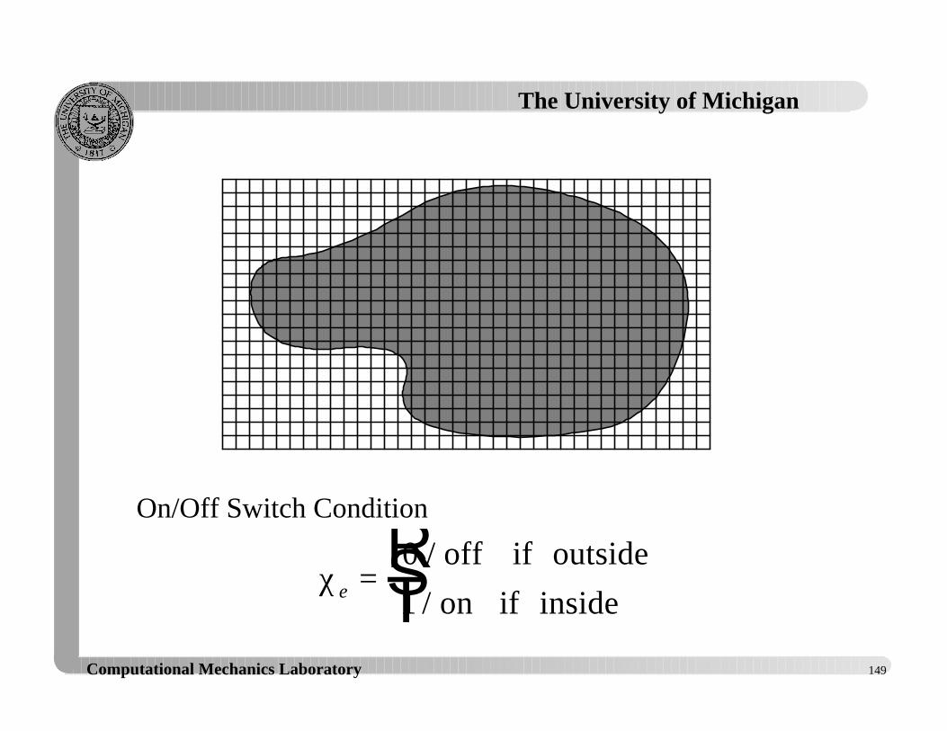
Characteristic Function

χΩ

ΩΩ

xx

xb g =

∈∉

RST1

0

if

if

On-Off condition for the unknown domain

Extended Formulation

ε ε ε εv E u v E ub g b g b g b gT T

Dd dDΩ

Ω Ωz z= χ

D

a priori

⊂ Ω is the extended design domain

that is fixed and known

149



χe =RST0

1

/

/

off if outside

on if inside

On/Off Switch Condition

150



What this means ?

ε ε ε εv E u v E ub g b g b g b gT

D

T

DdD dDχΩ Ωz z=

E EΩ Ω= =χ new material constants

Shape design can be transformed into design ofmaterial constants ( material distribution overa fixed design domain )

No mesh adaptation is required !

151



Look at Taylor’s Approach

Plate Thickness Optimization for Plane Elasticityby John E. Taylor in 1967

ε εv x E ub g b g4 b gT

Dh dD

Plate Thickness Designed

z

ε εv E ub g 0 b gT

DdDχΩ

Extended Domain Approach

z2D

2D & 3D

152



Pixel/Voxel Representation

on off

Shape is represented by a collection of pixels/voxelsas in monitors of computer graphics

153



OPTISHAPE

is a program based on this idea

image (pixel/voxel) based

representation of the shape

154



Very Flexible & Simple

Generating holes inside is not a problem !

that is not only SHAPE but also TOPOLOGYof a structure can be designed in this approach

155



OPTISHAPE

for

Shape Optimization

and

Topology Optimization

156




Simplified Rear Trunk Shell

Three Point Supports

Load Cases 1) Uniform Pressure on the Upper Plate 2) Point Loads at A and B independently when support 3 fails 3) Distributed Edge Load on Line a-a when support 3 fails

a a

1 2

3A B

Three Dimensional Design Domain Underthe Upper Plate (Discretized by 50x30x4 Mesh)

Documents

Computer Aided Engineering and OPTISHAPE