Embed Size (px)
Citation preview
COMPUTATIONAL FLUID DYNAMIC ANALYSIS OF
HIGHWAY BRIDGE SUPERSTRUCTURES
EXPOSED TO HURRICANE WAVES
by
Mehrdad Bozorgnia
A Dissertation Presented to the
FACULTY OF THE USC GRADUATE SCHOOL
UNIVERSITY OF SOUTHERN CALIFORNIA
In Partial Fulfillment of the
Requirements for the Degree
DOCTOR OF PHILOSOPHY
(CIVIL ENGINEERING)
December 2012
Copyright 2012 Mehrdad Bozorgnia

I would like to dedicate this dissertation work to my beloved family.
ii
Acknowledgments
Many people have provided their help and encouragement during this dissertation study.
This work would not have been done without them. I like to specially thank my advisor,
Professor Jiin-Jen Lee, who not only gave me the great opportunity to pursue a Ph.D.
degree at the University of Southern California, but also provided invaluable advice,
assistance, and encouragement throughout the whole study.
I also like to thank other members of the dissertation committee, Professors Carter
Wellford, Vincent Lee, and Iraj Nasseri in the Department of Civil and Environmental
Engineering and Professor James Moore in the Department of Industrial and System
Engineering at USC, for their guidance and help.
I would like to thank all of my past and present group members: Jen Chang, Chanin
Chaun-Im, Marmar Ghadiri, Ziyi Huang, Hyoung-Jin Kim, Zhiqing Kou, Shentong Lu,
Yuan-Hung Tan, Ben Willardson, and Xiuying Xing (following the alphabetic sequence
of the last names, no special order) for their incessant help and the warm atmosphere
they provided since I came to USC.
I would like to thank High-Performance Computing and Communications staff espe-
cially, Brian Mendenhall for his countless hours of assistance in setting up the CFD
software on HPCC Linux cluster and for continuous support and assistance throughout
different phases of this thesis.
iii

I would like to thank Shane Gillis from CD-adapco for his valuable advice regarding
application of the CFD software to wave-bridge interaction problem and for continuous
support and assistance throughout different phases of this thesis.
My very special thanks goes to my parents Fatemeh Sakhdari and Ahmad Bozorg-
nia, and my lovely sister Dr. Mehrshid Bozorgnia and all those with whom I have shared
my life in the past five years. In particular I would like to thank Hossein Ataei, Hos-
sein Hayati, Reza Jafarkhani, Mohammadreza Jahanshahi, Hadi Meidani, and Arash
Noshadravan. I wish you a life full of success, health and happiness.
iv
Contents
Dedication ii
Acknowledgments iii
List of Figures viii
List of Tables xiii
List of Notations xiv
Abstract xvi
Chapter 1 INTRODUCTION 1
1.1 Background . . . . . . . . . . . . . . . . . . . . . . . . . . . . . . . . 1
1.2 Objective and Scope of Present Study . . . . . . . . . . . . . . . . . . 5
Chapter 2 LITERATURE SURVEY 7
Chapter 3 MATHEMATICAL FORMULATION OF PROBLEM 16
3.1 Introduction . . . . . . . . . . . . . . . . . . . . . . . . . . . . . . . . 16
3.2 Governing Equations . . . . . . . . . . . . . . . . . . . . . . . . . . . 16
3.3 Discretization . . . . . . . . . . . . . . . . . . . . . . . . . . . . . . . 18
3.3.1 Momentum Equation in Discrete Form . . . . . . . . . . . . . . 19
3.3.2 Continuity Equation in Discrete Form . . . . . . . . . . . . . . . 20
3.4 SIMPLE Solver Algorithm . . . . . . . . . . . . . . . . . . . . . . . . 22
3.5 Numerical Method for Solving Algebraic Equations . . . . . . . . . . . 24
3.6 Multigrid Concept . . . . . . . . . . . . . . . . . . . . . . . . . . . . 26
3.7 Multiphase Methods . . . . . . . . . . . . . . . . . . . . . . . . . . . 30
Chapter 4 MODEL VALIDATION FOR UPLIFT FORCES ON FLAT PLATE 34
4.1 Solitary Wave . . . . . . . . . . . . . . . . . . . . . . . . . . . . . . . 34
4.2 Interaction of Solitary Wave with Platform over Horizontal Bottom . . 36
v
Chapter 5 EXPERIMENTAL SETUP AND NUMERICAL METHODOL-
OGY 41
5.1 Experimental Setup . . . . . . . . . . . . . . . . . . . . . . . . . . . . 42
5.2 Computation on High Performance Computing and Communications
Center (HPCC) at USC . . . . . . . . . . . . . . . . . . . . . . . . . . 48
5.3 Numerical Methodology and Solver Parameters . . . . . . . . . . . . . 53
5.4 Choice of Wave Profile . . . . . . . . . . . . . . . . . . . . . . . . . . 54
5.5 Choice of Boundary Conditions . . . . . . . . . . . . . . . . . . . . . 56
5.6 Choice of Mesh Size and Time Step . . . . . . . . . . . . . . . . . . . 57
5.7 Solution Convergence . . . . . . . . . . . . . . . . . . . . . . . . . . 63
5.8 Spectral Analysis . . . . . . . . . . . . . . . . . . . . . . . . . . . . . 66
5.9 Slamming Force and Structural Response . . . . . . . . . . . . . . . . 67
Chapter 6 NUMERICAL RESULTS FOR LARGE SCALE WAVE BRIDGE
INTERACTION 73
6.1 2D Model . . . . . . . . . . . . . . . . . . . . . . . . . . . . . . . . . 73
6.1.1 Simulation Results for Test #1 . . . . . . . . . . . . . . . . . . . 74
6.1.2 Simulation Results for Test #2 . . . . . . . . . . . . . . . . . . . 77
6.1.3 Simulation Results for Test #3 . . . . . . . . . . . . . . . . . . . 85
6.2 3D Model . . . . . . . . . . . . . . . . . . . . . . . . . . . . . . . . . 90
6.2.1 Simulation Results for Test #4 . . . . . . . . . . . . . . . . . . . 92
6.2.2 Simulation Results for Test #5 . . . . . . . . . . . . . . . . . . . 95
6.2.3 Simulation Results for Test #6 . . . . . . . . . . . . . . . . . . . 98
6.3 Discussion on Slamming Force . . . . . . . . . . . . . . . . . . . . . 111
6.4 Discussion on Simulation Results . . . . . . . . . . . . . . . . . . . . 114
6.5 Guidelines for Choosing Mesh and Time Step Size in Wave-Structure
Interaction Problems . . . . . . . . . . . . . . . . . . . . . . . . . . . 117
6.6 Viscous Effects . . . . . . . . . . . . . . . . . . . . . . . . . . . . . . 118
Chapter 7 SCALE EFFECTS ON HYDRODYNAMIC FORCES AND COM-
PARISON OF SIMULATED FORCES TO AASHTO GUIDE-
LINES 123
7.1 Scale Effects . . . . . . . . . . . . . . . . . . . . . . . . . . . . . . . 123
7.2 AASHTO Guidelines . . . . . . . . . . . . . . . . . . . . . . . . . . . 132
7.3 Comparison of Simulated Wave Forces to AASHTO Guidelines . . . . 135
Chapter 8 RETROFITTING OPTIONS AVAILABLE FOR COASTAL BRIDGES
EXPOSED TO WAVES 140
8.1 Airvents in Bridge Deck . . . . . . . . . . . . . . . . . . . . . . . . . 141
8.2 Airvents in Bridge Diaphragm . . . . . . . . . . . . . . . . . . . . . . 148
Chapter 9 CONCLUDING REMARKS 153
vi
Reference List 159
Appendix ADISCRETIZATION SCHEMES USED IN STAR CCM+ 163
A.1 Transport Equation in Discrete Form . . . . . . . . . . . . . . . . . . 163
A.2 Gradient Computation . . . . . . . . . . . . . . . . . . . . . . . . . . 166
vii

List of Figures
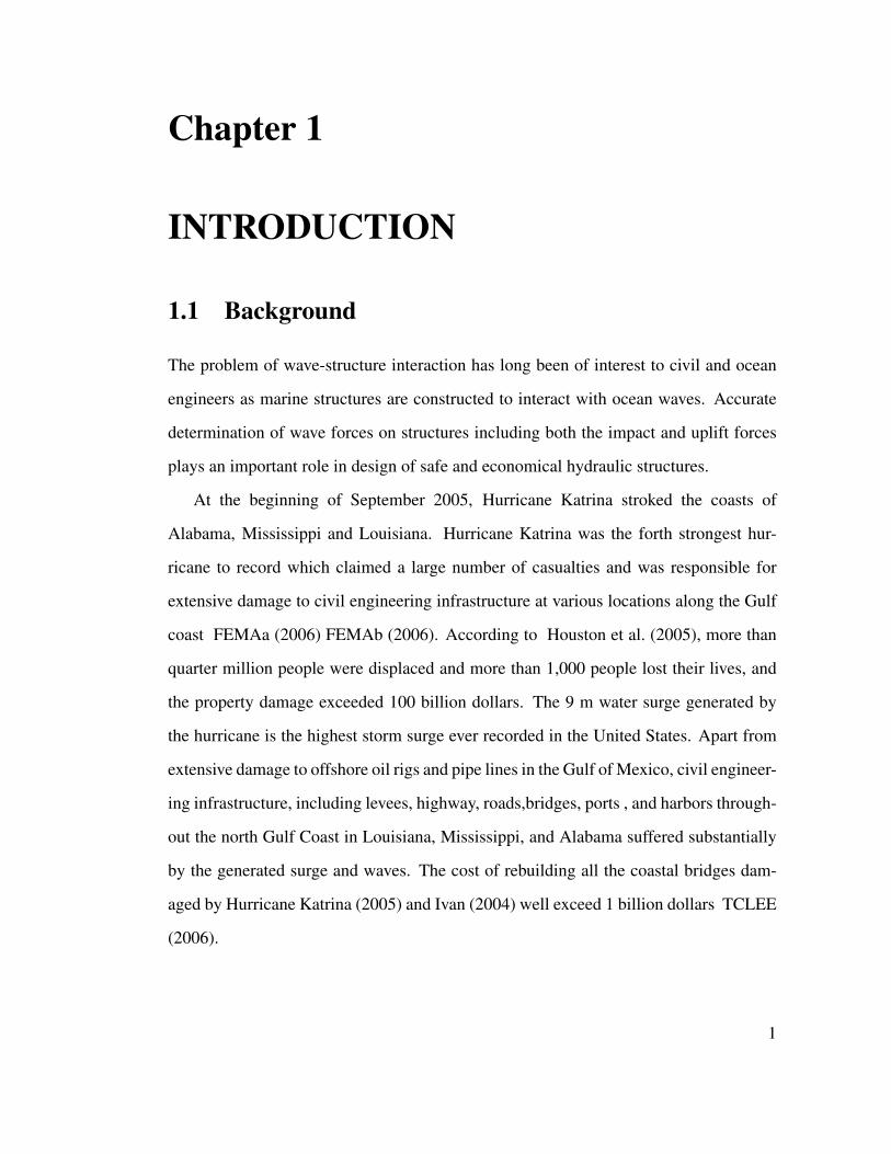
1.1 Damage to the U.S. 90 Biloxi Bay bridge caused by Hurricane Katrina.
This photo is taken looking northeast from Biloxi 9/21/05 (source Dou-
glass et al. (2006)). . . . . . . . . . . . . . . . . . . . . . . . . . . . . 2
1.2 I-10 bridge, Mobile Bay, Alabama, damaged by Hurricane Katrina (source
Douglass et al. (2006)). . . . . . . . . . . . . . . . . . . . . . . . . . . 3
1.3 I-10 bridge over Escambia Bay, Florida, damaged by Hurricane Ivan
(Pensacola News Journal photo). . . . . . . . . . . . . . . . . . . . . . 3
3.1 A typical CV and the notation used for cartesian 2D grid . . . . . . . . 18
3.2 Residual reduction pattern by iterative solver for different grid resolu-
tions (adapted from Versteeg and Malalasekera (2007)) . . . . . . . . . 27
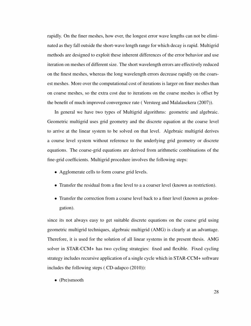
3.3 V-cycle adapted from CD-adapco (2010) . . . . . . . . . . . . . . . . 29
3.4 Illustration of girds that are suitable (right) and unsuitable (left) for two
phase flows using VOF model adapted from CD-adapco (2010) . . . . 31
3.5 Upwind, downwind and central cells used in the analysis (left) and con-
vection boundedness criterion in the NVD diagram (right) adapted from
CD-adapco (2010) . . . . . . . . . . . . . . . . . . . . . . . . . . . . . 33
3.6 a)True interface b)Volume Fraction . . . . . . . . . . . . . . . . . . . . 33
4.1 Experimental setup (French 1969) for numerical model validation . . . 36
4.2 Mesh used in the simulation . . . . . . . . . . . . . . . . . . . . . . . . 37
4.3 Horizontal water particle velocities H/d=0.15,s/d=0.1,y/d=0.0,d=12”,L=2” 37
4.4 Horizontal water particle velocities H/d=0.15,s/d=0.1,y/d=-0.5,d=12”,L=2” 38
4.5 Normalized total hydrodynamic force per unit width H/d=0.24, s/d=0.2,
L/d=4, d=15” . . . . . . . . . . . . . . . . . . . . . . . . . . . . . . . 39
4.6 Normalized total hydrodynamic force per unit width H/d=0.32, s/d=0.2,
L/d=4, d=15” . . . . . . . . . . . . . . . . . . . . . . . . . . . . . . . 39
4.7 Normalized total hydrodynamic force per unit width H/d=0.4, s/d=0.2,
L/d=4, d=15” . . . . . . . . . . . . . . . . . . . . . . . . . . . . . . . 40
5.1 Elevation view of typical prototype bridge (courtesy of Thomas Schu-
macher, Oregon State University.) . . . . . . . . . . . . . . . . . . . . 41
5.2 Elevation view of wave flume with experimental setup (courtesy of Thomas
Schumacher, Oregon State University). . . . . . . . . . . . . . . . . . . 42
viii
5.3 Pre-cast bridge specimen prior to attachment of deck ( Bradner and Cox
(2008)). . . . . . . . . . . . . . . . . . . . . . . . . . . . . . . . . . . 43
5.4 Test setup installed in Large Wave Flume ( Bradner and Cox (2008)) . . 44
5.5 Elevation view (side) of test specimen and reaction frame along with
horizontal and vertical load cells ( Bradner and Cox (2008)) . . . . . . . 45
5.6 Instrumentation plan for pressure gages and load cells; plan view ( Brad-
ner and Cox (2008)). . . . . . . . . . . . . . . . . . . . . . . . . . . . 45
5.7 Photo of the bridge specimen during wave trial ( Bradner and Cox (2008)). 46
5.8 Time series of total horizontal force (LC1+LC2) for wave trial 1325.
Markers indicate data points used to compute mean positive and negative
peak forces ( Bradner and Cox (2008)). . . . . . . . . . . . . . . . . . . 47
5.9 Time series of total vertical force (LC3+LC4+LC5+LC6) for wave trial
1325. Markers indicate data points used to compute mean positive and
negative peak forces ( Bradner and Cox (2008)). . . . . . . . . . . . . . 47
5.10 Horizontal and vertical reaction forces for various wave heights for T=2.5s
( Schumacher et al. (2008)). . . . . . . . . . . . . . . . . . . . . . . . . 48
5.11 HPCC at USC. . . . . . . . . . . . . . . . . . . . . . . . . . . . . . . . 49
5.12 Relationship between client and parallel server adapted from ( CD-adapco
(2010)) . . . . . . . . . . . . . . . . . . . . . . . . . . . . . . . . . . . 50
5.13 Script used for submitting the CFD job to HPCC Linux cluster . . . . . 51
5.14 Number of CPU per node vs speed-up . . . . . . . . . . . . . . . . . . 52
5.15 Total number of CPU vs speed-up . . . . . . . . . . . . . . . . . . . . 52
5.16 Applicability ranges of various wave theories (after Mhaut et al. (1968)).
d: mean water depth; H: wave height; T: wave period; g: gravitational
acceleration. . . . . . . . . . . . . . . . . . . . . . . . . . . . . . . . . 55
5.17 Incident wave generated using stokes fifth order theory for H=0.5m and
T=2.5 s . . . . . . . . . . . . . . . . . . . . . . . . . . . . . . . . . . 56
5.18 Boundary Conditions used in 2D simulation cases . . . . . . . . . . . . 57
5.19 Mesh regions . . . . . . . . . . . . . . . . . . . . . . . . . . . . . . . 58
5.20 Simulation domain dimension . . . . . . . . . . . . . . . . . . . . . . 58
5.21 Effect of time step choice on total horizontal wave forces for dt=0.02s
and dt=0.004s . . . . . . . . . . . . . . . . . . . . . . . . . . . . . . . 61
5.22 Effect of time step choice on total vertical wave forces for dt=0.02s and
dt=0.004s . . . . . . . . . . . . . . . . . . . . . . . . . . . . . . . . . 61
5.23 Convective Courant Number for Test #6 . . . . . . . . . . . . . . . . . 62
5.24 Residuals for continuity and momentum equations . . . . . . . . . . . . 64
5.25 Convergence in several time steps . . . . . . . . . . . . . . . . . . . . 65
5.26 Convergence in one time step . . . . . . . . . . . . . . . . . . . . . . . 65
5.27 Vertical force reaching asymptotic limit in one time step before going to
next time step . . . . . . . . . . . . . . . . . . . . . . . . . . . . . . . 65
5.28 Horizontal force power spectral density . . . . . . . . . . . . . . . . . 66
5.29 Vertical force power spectral density . . . . . . . . . . . . . . . . . . . 67
ix
5.30 Typical vertical wave force versus time plot for a subaerial structure with
girders adapted from ( FDOT (2008)). . . . . . . . . . . . . . . . . . . 67
5.31 Spring-mass-dashpot system . . . . . . . . . . . . . . . . . . . . . . . 69
5.32 Amplitude amplification as a function of forcing frequency and damping 70
5.33 Example of filtered and unfiltered vertical force for a subaerial slab. . . 70
5.34 Quasi steady vs. raw horizontal wave forces . . . . . . . . . . . . . . . 71
5.35 Quasi steady vs. raw vertical wave forces . . . . . . . . . . . . . . . . 72
6.1 Horizontal force simulation results for Test #1 . . . . . . . . . . . . . . 75
6.2 Vertical force simulation results for Test #1 . . . . . . . . . . . . . . . 76
6.3 Comparison of horizontal and vertical simulation wave forces for Test
#1 to experimental data . . . . . . . . . . . . . . . . . . . . . . . . . . 76
6.4 Horizontal force simulation results for Test #2 . . . . . . . . . . . . . . 77
6.5 Vertical force simulation results for Test #2 . . . . . . . . . . . . . . . 79
6.6 Comparison of horizontal and vertical simulation wave forces for Test
#2 to experimental data . . . . . . . . . . . . . . . . . . . . . . . . . . 79
6.7 Volume of fluid (VOF) scene for H=0.84m (Test #2) . . . . . . . . . . . 81
6.8 Absolute pressure scene for H=0.84m (Test #2) . . . . . . . . . . . . . 82
6.9 Velocity vector scene for H=0.84m (Test #2) . . . . . . . . . . . . . . . 83
6.10 Velocity magnitude in horizontal direction for H=0.84m (Test #2) . . . . 84
6.11 Velocity magnitude in vertical direction for H=0.84m (Test #2) . . . . . 85
6.12 Horizontal force simulation results for Test #3 . . . . . . . . . . . . . . 87
6.13 Vertical force simulation results for Test #3 . . . . . . . . . . . . . . . 88
6.14 Comparison of horizontal and vertical simulation wave forces for Test
#3 to experimental data . . . . . . . . . . . . . . . . . . . . . . . . . . 88
6.15 Volume of fluid (VOF) scene for H=0.84m, dt=0.02 (Test #3) . . . . . . 89
6.16 Meshed bridge in full 3D model . . . . . . . . . . . . . . . . . . . . . 90
6.17 Meshed bridge in 3D model with symmetry plane . . . . . . . . . . . . 90
6.18 Comparison of total horizontal force in the full bridge superstructure
model to the bridge superstructure model with symmetry plane . . . . . 91
6.19 Comparison of total vertical force in the full bridge superstructure model
to the bridge superstructure model with symmetry plane . . . . . . . . . 91
6.20 Horizontal force simulation results for Test #4 . . . . . . . . . . . . . . 93
6.21 Vertical force simulation results for Test #4 . . . . . . . . . . . . . . . 94
6.22 Comparison of horizontal and vertical simulation wave forces for Test
#4 to experimental data . . . . . . . . . . . . . . . . . . . . . . . . . . 94
6.23 Horizontal force simulation results for Test #5 . . . . . . . . . . . . . . 96
6.24 Vertical force simulation results for Test #5 . . . . . . . . . . . . . . . 97
6.25 Comparison of horizontal and vertical simulation wave forces for Test
#5 to experimental data . . . . . . . . . . . . . . . . . . . . . . . . . . 97
6.26 Horizontal force simulation results for Test #6 . . . . . . . . . . . . . . 99
6.27 Vertical force simulation results for Test #6 . . . . . . . . . . . . . . . 100
x
6.28 Comparison of horizontal and vertical simulation wave forces to exper-
imental data for Test #6 . . . . . . . . . . . . . . . . . . . . . . . . . . 100
6.29 Comparison of positive and negative horizontal forces to experimental
data . . . . . . . . . . . . . . . . . . . . . . . . . . . . . . . . . . . . 101
6.30 Comparison of positive and negative vertical forces to experimental data 102
6.31 Error distribution for quasi-steady horizontal wave forces for Test #6 . . 102
6.32 Error distribution for quasi-steady vertical wave forces for Test #6 . . . 103
6.33 Volume of fluid (VOF) scene for H=0.84m (Test #6) . . . . . . . . . . . 105
6.34 Pressure scene for H=0.84m (Test #6) . . . . . . . . . . . . . . . . . . 106
6.35 Velocity vector scene for H=0.84m (Test #6) . . . . . . . . . . . . . . . 107
6.36 Velocity magnitude in horizontal direction for H=0.84m (Test #6) . . . . 108
6.37 Velocity magnitude in vertical direction for H=0.84m (Test #6) . . . . . 109
6.38 3D iso surface for H=0.84m (Test #6) . . . . . . . . . . . . . . . . . . 110
6.39 Pressure measurement taken beneath the deck adapted from Bradner
and Cox (2008) . . . . . . . . . . . . . . . . . . . . . . . . . . . . . . 111
6.40 Corresponding measurement of the nearest load cell adapted from Brad-
ner and Cox (2008) . . . . . . . . . . . . . . . . . . . . . . . . . . . . 111
6.41 Vertical force time history for one wave period for Test #6 for different
wave heights . . . . . . . . . . . . . . . . . . . . . . . . . . . . . . . . 113
6.42 Effect of model choice and mesh size on magnitude of slamming force
oscillation . . . . . . . . . . . . . . . . . . . . . . . . . . . . . . . . . 113
6.43 Comparison of horizontal forces using SST K-Omega model to inviscid
model for H=0.34m for Test #6 . . . . . . . . . . . . . . . . . . . . . . 120
6.44 Comparison of vertical forces using SST K-Omega model simulation to
inviscid model for H=0.34m for Test #6 . . . . . . . . . . . . . . . . . 121
6.45 Comparison of vertical forces using SST K-Omega model simulation to
inviscid model for H=0.84m for Test #6 . . . . . . . . . . . . . . . . . 121
6.46 Comparison of vertical forces using SST K-Omega model simulation to
inviscid model for H=0.84m for Test #6 . . . . . . . . . . . . . . . . . 122
7.1 Horizontal force simulation results for prototype bridge vs. results archived
from model bridge using Froude similitude law . . . . . . . . . . . . . 126
7.2 Vertical force simulation results for prototype bridge vs. results archived
from model bridge using Froude similitude law . . . . . . . . . . . . . 127
7.3 Volume of fluid (VOF) scenes for H=4.2m wave interacting with proto-
type bridge . . . . . . . . . . . . . . . . . . . . . . . . . . . . . . . . . 128
7.4 Pressure scenes for H=4.2m wave interacting with prototype bridge . . . 129
7.5 Velocity magnitude in horizontal direction for H=4.2m wave interacting
with prototype bridge . . . . . . . . . . . . . . . . . . . . . . . . . . . 130
7.6 Velocity magnitude in vertical direction for H=4.2m wave interacting
with prototype bridge . . . . . . . . . . . . . . . . . . . . . . . . . . . 131
7.7 Nomenclature in equation 7.3 and 7.2 adapted from AASHTO (2008) . 134
xi
7.8 Comparison of simulated forces for model bridge to AASHTO guideline 136
7.9 Comparison of simulated quasi-steady forces for model bridge to AASHTO
guideline . . . . . . . . . . . . . . . . . . . . . . . . . . . . . . . . . . 137
7.10 Comparison of simulated forces for prototype bridge to AASHTO guide-
line . . . . . . . . . . . . . . . . . . . . . . . . . . . . . . . . . . . . . 138
7.11 Comparison of simulated quasi-steady forces for prototype bridge to
AASHTO guideline . . . . . . . . . . . . . . . . . . . . . . . . . . . . 138
8.1 Retrofit option 1 . . . . . . . . . . . . . . . . . . . . . . . . . . . . . . 141
8.2 Volume of fluid (VOF) scene for option 1 . . . . . . . . . . . . . . . . 142
8.3 3D iso surface for option 1 . . . . . . . . . . . . . . . . . . . . . . . . 143
8.4 Effect of option 1 retrofit on horizontal force time history for H=0.34m 145
8.5 Effect of option 1 retrofit on horizontal force time history for H=0.84m . 145
8.6 Effect of option 1 retrofit on vertical force time history for H=0.34m . . 146
8.7 Effect of option 1 retrofit on vertical force time history for H=0.84m . . 146
8.8 Effect of option 1 retrofit on horizontal force for various wave heights . 147
8.9 Effect of option 1 retrofit on vertical force for various wave heights . . . 148
8.10 Retrofit option 2 . . . . . . . . . . . . . . . . . . . . . . . . . . . . . . 149
8.11 Effect of option 2 retrofit on horizontal force time history for H=0.34m . 150
8.12 Effect of option 2 retrofit on horizontal force time history for H=0.84m . 150
8.13 Effect of option 2 retrofit on vertical force time history for H=0.34m . . 151
8.14 Effect of option 2 retrofit on vertical force time history for H=0.84m . . 151
8.15 Effect of option 2 retrofit on horizontal force for various wave heights . 152
8.16 Effect of option 1 retrofit on vertical force for various wave heights . . . 152
A.1 decomposition used in calculation of Diffusion term . . . . . . . . . . . 165
xii
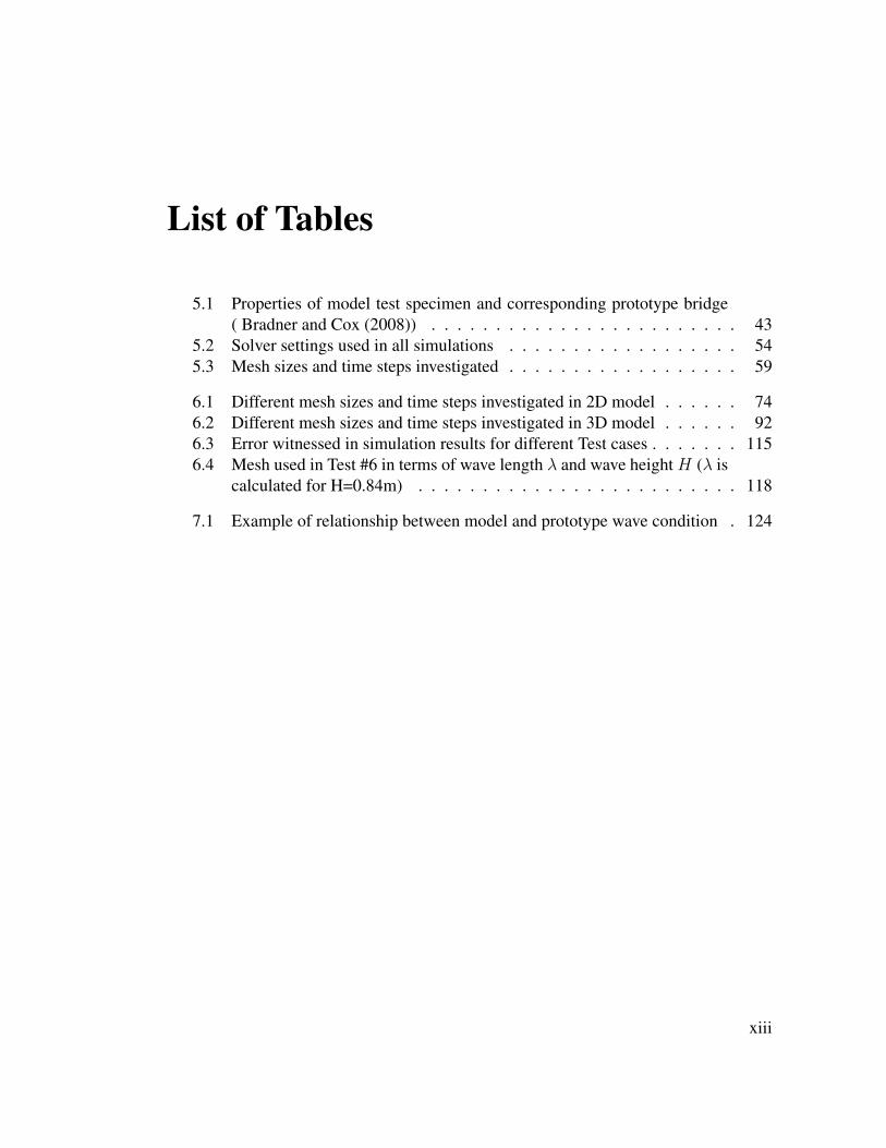
List of Tables
5.1 Properties of model test specimen and corresponding prototype bridge
( Bradner and Cox (2008)) . . . . . . . . . . . . . . . . . . . . . . . . 43
5.2 Solver settings used in all simulations . . . . . . . . . . . . . . . . . . 54
5.3 Mesh sizes and time steps investigated . . . . . . . . . . . . . . . . . . 59
6.1 Different mesh sizes and time steps investigated in 2D model . . . . . . 74
6.2 Different mesh sizes and time steps investigated in 3D model . . . . . . 92
6.3 Error witnessed in simulation results for different Test cases . . . . . . . 115
6.4 Mesh used in Test #6 in terms of wave length λ and wave height H (λ is
calculated for H=0.84m) . . . . . . . . . . . . . . . . . . . . . . . . . 118
7.1 Example of relationship between model and prototype wave condition . 124
xiii
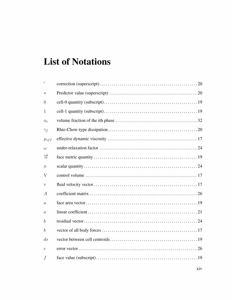
List of Notations
′ correction (superscript) . . . . . . . . . . . . . . . . . . . . . . . . . . . . . . . . . . . . . . . . . . . . . . . . . 20
∗ Predictor value (superscript) . . . . . . . . . . . . . . . . . . . . . . . . . . . . . . . . . . . . . . . . . . . . 20
0 cell-0 quantity (subscript) . . . . . . . . . . . . . . . . . . . . . . . . . . . . . . . . . . . . . . . . . . . . . . . 19
1 cell-1 quantity (subscript) . . . . . . . . . . . . . . . . . . . . . . . . . . . . . . . . . . . . . . . . . . . . . . . 19
αi volume fraction of the ith phase . . . . . . . . . . . . . . . . . . . . . . . . . . . . . . . . . . . . . . . . . 32
γf Rhie-Chow-type dissipation . . . . . . . . . . . . . . . . . . . . . . . . . . . . . . . . . . . . . . . . . . . . . 20
µeff effective dynamic viscosity . . . . . . . . . . . . . . . . . . . . . . . . . . . . . . . . . . . . . . . . . . . . . 17
ω under-relaxation factor . . . . . . . . . . . . . . . . . . . . . . . . . . . . . . . . . . . . . . . . . . . . . . . . . 24
−→α face metric quantity . . . . . . . . . . . . . . . . . . . . . . . . . . . . . . . . . . . . . . . . . . . . . . . . . . . . 19
φ scalar quantity . . . . . . . . . . . . . . . . . . . . . . . . . . . . . . . . . . . . . . . . . . . . . . . . . . . . . . . . . 24
V control volume . . . . . . . . . . . . . . . . . . . . . . . . . . . . . . . . . . . . . . . . . . . . . . . . . . . . . . . . 17
v fluid velocity vector . . . . . . . . . . . . . . . . . . . . . . . . . . . . . . . . . . . . . . . . . . . . . . . . . . . . 17
A coefficient matrix . . . . . . . . . . . . . . . . . . . . . . . . . . . . . . . . . . . . . . . . . . . . . . . . . . . . . . 26
a face area vector . . . . . . . . . . . . . . . . . . . . . . . . . . . . . . . . . . . . . . . . . . . . . . . . . . . . . . . . 19
a linear coefficient . . . . . . . . . . . . . . . . . . . . . . . . . . . . . . . . . . . . . . . . . . . . . . . . . . . . . . . 21
b residual vector . . . . . . . . . . . . . . . . . . . . . . . . . . . . . . . . . . . . . . . . . . . . . . . . . . . . . . . . . 24
b vector of all body forces . . . . . . . . . . . . . . . . . . . . . . . . . . . . . . . . . . . . . . . . . . . . . . . . 17
ds vector between cell centroids . . . . . . . . . . . . . . . . . . . . . . . . . . . . . . . . . . . . . . . . . . . .19
e error vector . . . . . . . . . . . . . . . . . . . . . . . . . . . . . . . . . . . . . . . . . . . . . . . . . . . . . . . . . . . 26
f face value (subscript) . . . . . . . . . . . . . . . . . . . . . . . . . . . . . . . . . . . . . . . . . . . . . . . . . . . 19
xiv

I identity matrix . . . . . . . . . . . . . . . . . . . . . . . . . . . . . . . . . . . . . . . . . . . . . . . . . . . . . . . . . 17
k iteration k (superscript) . . . . . . . . . . . . . . . . . . . . . . . . . . . . . . . . . . . . . . . . . . . . . . . . . 24
n neighbor coefficient (subscript) . . . . . . . . . . . . . . . . . . . . . . . . . . . . . . . . . . . . . . . . . . 21
p center coefficient (subscript) . . . . . . . . . . . . . . . . . . . . . . . . . . . . . . . . . . . . . . . . . . . . 21
p pressure . . . . . . . . . . . . . . . . . . . . . . . . . . . . . . . . . . . . . . . . . . . . . . . . . . . . . . . . . . . . . . .19
r residual (scalar) . . . . . . . . . . . . . . . . . . . . . . . . . . . . . . . . . . . . . . . . . . . . . . . . . . . . . . . .21
T iteration matrix . . . . . . . . . . . . . . . . . . . . . . . . . . . . . . . . . . . . . . . . . . . . . . . . . . . . . . . . 26
T viscous stress tensor . . . . . . . . . . . . . . . . . . . . . . . . . . . . . . . . . . . . . . . . . . . . . . . . . . . .17
t time . . . . . . . . . . . . . . . . . . . . . . . . . . . . . . . . . . . . . . . . . . . . . . . . . . . . . . . . . . . . . . . . . . 17
x solution vector . . . . . . . . . . . . . . . . . . . . . . . . . . . . . . . . . . . . . . . . . . . . . . . . . . . . . . . . .26
y approximate solution vector . . . . . . . . . . . . . . . . . . . . . . . . . . . . . . . . . . . . . . . . . . . . . 26
ρ fluid density . . . . . . . . . . . . . . . . . . . . . . . . . . . . . . . . . . . . . . . . . . . . . . . . . . . . . . . . . . . 17
vg grid velocity . . . . . . . . . . . . . . . . . . . . . . . . . . . . . . . . . . . . . . . . . . . . . . . . . . . . . . . . . . . 17
Gf grid flux . . . . . . . . . . . . . . . . . . . . . . . . . . . . . . . . . . . . . . . . . . . . . . . . . . . . . . . . . . . . . . 20
Qf coefficient in dissipation . . . . . . . . . . . . . . . . . . . . . . . . . . . . . . . . . . . . . . . . . . . . . . . . 20
mf face mass flow . . . . . . . . . . . . . . . . . . . . . . . . . . . . . . . . . . . . . . . . . . . . . . . . . . . . . . . . . 20
xv
Abstract
Highway bridges are one of the most vulnerable critical components of transportation
system. Several coastal highway bridges were severely damaged during past hurricanes
due to hurricane induced storm surge. The total cost of bridge repair or replacement
after Hurricane Katrina was estimated to exceed 1 billion dollar TCLEE (2006).
The objective of this study is to calculate the hydrodynamic forces applied to bridge
superstructure due to hurricane induced wave via Computational Fluid Dynamic (CFD)
with an emphasis on the effect of air entrapment under highway bridge superstructure.
Three dimensional numerical wave-load model based on two-phase Navier-Stokes equa-
tions is used to evaluate dynamic wave forces exerted on the bridge deck. In order to
accurately capture the complex interaction of waves with bridge deck, several millions
of mesh cells are used in the simulation domain and simulations are ran on High Perfor-
mance Computing and Communication Center (HPCC) cluster at University of Southern
California.
First, CFD software was validated by simulating interaction of a solitary wave with
a flat plate. The simulation results for pressure under the plate and velocities at different
points inside the simulation domain were compared with experimental data available
from French (1970).
Second, validated numerical model was applied to a 1:5 scale old Escambia Bay
bridge which was heavily damaged during Hurricane Ivan. Compared to simple flat
xvi
plate problem, Highway bridge superstructure is more challenging due to its complex
geometry, bluff profile, and other complexities rising from trapped air under bridge
superstructure, turbulence, structural response and scale effects. Simulation results were
compared to experimental data available from the O.H. Hinsdale Wave Research Labo-
ratory at Oregon State University. Influence of modeling (2D vs 3D), time step, grid size
and viscous effects on total hydrodynamic forces applied to highway bridge superstruc-
ture have been investigated. Some guidelines based on simulation results are developed
for the best mesh configuration and optimum choice of mesh size and time step for
similar wave-structure interaction problems.
Third, in order to evaluate scale effects in the wave-bridge interaction problem, a
bridge prototype with exact old Escambia Bay Bridge dimensions is setup. Equiva-
lent wave heights and period are calculated using Froude similitude laws from the wave
heights and periods used in model simulations. The forces obtained from CFD simula-
tions for prototype bridge are compared to forces calculated using Froude similitude law
from model bridge simulations. Next, CFD simulation results for model and prototype
bridge are compared with recently published AASHTO guidelines for coastal bridges
vulnerable to storms ( AASHTO (2008)).
Forth, since air entrapped between bridge girders and diaphragm was determined
to be a major contributing factor behind many highway bridge failures during recent
hurricanes , two retrofitting options are evaluated in terms of their efficacy in reducing
hydrodynamics forces applied to bridge superstructure. These two options include using
airvents in bridge deck and using airvents in bridge diaphragms.
xvii
Chapter 1
INTRODUCTION
1.1 Background
The problem of wave-structure interaction has long been of interest to civil and ocean
engineers as marine structures are constructed to interact with ocean waves. Accurate
determination of wave forces on structures including both the impact and uplift forces
plays an important role in design of safe and economical hydraulic structures.
At the beginning of September 2005, Hurricane Katrina stroked the coasts of
Alabama, Mississippi and Louisiana. Hurricane Katrina was the forth strongest hur-
ricane to record which claimed a large number of casualties and was responsible for
extensive damage to civil engineering infrastructure at various locations along the Gulf
coast FEMAa (2006) FEMAb (2006). According to Houston et al. (2005), more than
quarter million people were displaced and more than 1,000 people lost their lives, and
the property damage exceeded 100 billion dollars. The 9 m water surge generated by
the hurricane is the highest storm surge ever recorded in the United States. Apart from
extensive damage to offshore oil rigs and pipe lines in the Gulf of Mexico, civil engineer-
ing infrastructure, including levees, highway, roads,bridges, ports , and harbors through-
out the north Gulf Coast in Louisiana, Mississippi, and Alabama suffered substantially
by the generated surge and waves. The cost of rebuilding all the coastal bridges dam-
aged by Hurricane Katrina (2005) and Ivan (2004) well exceed 1 billion dollars TCLEE
(2006).
1
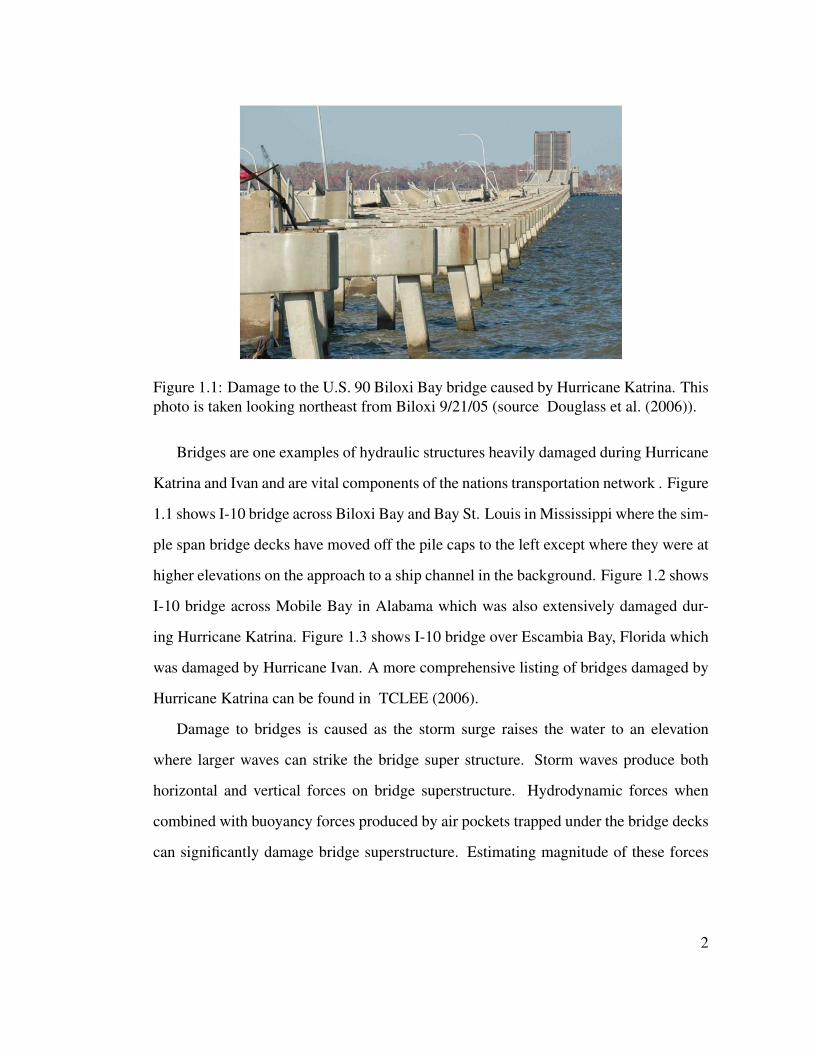
Figure 1.1: Damage to the U.S. 90 Biloxi Bay bridge caused by Hurricane Katrina. This
photo is taken looking northeast from Biloxi 9/21/05 (source Douglass et al. (2006)).
Bridges are one examples of hydraulic structures heavily damaged during Hurricane
Katrina and Ivan and are vital components of the nations transportation network . Figure
1.1 shows I-10 bridge across Biloxi Bay and Bay St. Louis in Mississippi where the sim-
ple span bridge decks have moved off the pile caps to the left except where they were at
higher elevations on the approach to a ship channel in the background. Figure 1.2 shows
I-10 bridge across Mobile Bay in Alabama which was also extensively damaged dur-
ing Hurricane Katrina. Figure 1.3 shows I-10 bridge over Escambia Bay, Florida which
was damaged by Hurricane Ivan. A more comprehensive listing of bridges damaged by
Hurricane Katrina can be found in TCLEE (2006).
Damage to bridges is caused as the storm surge raises the water to an elevation
where larger waves can strike the bridge super structure. Storm waves produce both
horizontal and vertical forces on bridge superstructure. Hydrodynamic forces when
combined with buoyancy forces produced by air pockets trapped under the bridge decks
can significantly damage bridge superstructure. Estimating magnitude of these forces
2
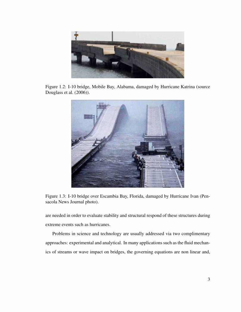
Figure 1.2: I-10 bridge, Mobile Bay, Alabama, damaged by Hurricane Katrina (source
Douglass et al. (2006)).
Figure 1.3: I-10 bridge over Escambia Bay, Florida, damaged by Hurricane Ivan (Pen-
sacola News Journal photo).
are needed in order to evaluate stability and structural respond of these structures during
extreme events such as hurricanes.
Problems in science and technology are usually addressed via two complimentary
approaches: experimental and analytical. In many applications such as the fluid mechan-
ics of streams or wave impact on bridges, the governing equations are non linear and,
3
except in special circumstances, analytical solution are not available. While, it is pos-
sible to address some of these problems through experiment, full scale experiments are
not usually possible for problems such as wave-bridge interaction because simply such
models can not be build in Lab environment. Therefore, researchers usually use smaller
scale and simplified representation of the physical configuration and extrapolate results
to apply to actual condition. Some degree of uncertainty will remain in this extrapola-
tion and use of simplified experiments to predict the behavior of the complex physical
system.
Recently, with the help of powerful supercomputers and Computational Fluid
Dynamic (CFD) programs, a third approach became available. CFD can complement
the experimental and analytical approaches by numerically solving the underlying gov-
erning equations that represent the flow of fluids. CFD enables scientists to model true
geometry of the given physical condition and can include actual observed boundary
condition that might be impossible to represent in laboratory experiments. In addition,
CFD allows for parametric studies on material properties and physical conditions that
might be expensive or time consuming to perform experimentally. CFD, also allows for
modeling various ”what-if” scenarios which might be very costly to do in laboratory
environment. CFD modeling should ideally include all of the physical processes such as
wave breaking, non linear effects, irregularity of waves, energy dissipations to friction
and turbulence, air entrapment and entrainment, etc... How ever, due to complexities
involved some degree of simplification is required to get solution to the problem. These
simplifications are discussed and justified in the following chapters.
4
1.2 Objective and Scope of Present Study
The major objective of the present study is to investigate the wave hydrodynamic effects
on highway bridge superstructures. A numerical wave-load model based on two- phase
Navier-Stokes type equations is used to evaluate dynamic wave forces exerted on these
hydraulic structures with special emphasis on the effect of air entrainment and entrap-
ment. The Volume of Fluid method (VOF) is adopted in the model to describe dynamic
free surface, which is capable of simulating complex discontinuous free surface associ-
ated with wave-deck interactions.
For present study the flow is assumed to be inviscid. Assumption of no viscously is
valid for present study, because we are dealing with large amplitude waves interaction
with bridge superstructure in a very short time. This makes the inertia term in Navier
Stokes equation much more important than viscous term and hence making the vis-
cous effect negligible. This assumption greatly simplifies our numerical discretization
schemes as allows for solving Euler equations instead of full Navier Stokes equations.
Chapter 2 includes brief review of previous numerical and experimental studies
about hydrodynamic forces on hydraulic structures. In Chapter 3 the mathematical
formulation of the problem is described which includes underlying equations and dis-
cretization schemes used to discretize these equations. Chapter 4 includes numerical
model validation for uplift forces on a flat plate. Chapter 5 Explains the experimen-
tal setup used at O.H. Hinsdale Wave Research Laboratory at Oregon State University
and solver settings and parameters used in the CFD software. Chapter 6 presents the
numerical results and their comparison to experimental data available from Oregon State
University. Chapter 7 investigates effects of scaling in wave-bridge interaction problem
and validity of Froude similitude law to extrapolate simulation results from model to
prototype. It also compares the simulation results for both model and prototype bridge
to the latest AASHTO guidelines. Chapter 8 explores retrofitting efficacy of some of
5
the retrofitting options recommended in literature to protect the bridges against violent
waves. Chapter 9 summarizes the findings of this dissertation.
6
Chapter 2
LITERATURE SURVEY
In this Chapter previous investigations on wave-structure interaction will be briefly
reviewed. Most of published research studies regarding wave forces on hydraulic struc-
tures is based on laboratory experiments.
El.Ghamry (1963) conducted extensive experiments on docks supported by piles
over flat and sloping bottoms. His experiments were conducted in a 105 ft long, 1 ft wide
wave flume with monochromatic waves with variable wave height, period and clearance
above the still water. El.Ghamry (1963) found that the force time history was a function
of wave period and elevation of the deck above still water. He also found that the force
time history consisted of positive uplift force due to boundary condition imposed on
velocity and negative uplift force associated with advance of the trough under the deck.
He then modified his experimental setup to quantify the role of entrapped air under the
deck by using structural members such as beams and diaphragms. He reported that for
certain wave periods, for slopping beach cases, air entrapment could cause impulsive
uplift forces up to 100 times greater than the loads measured in other tests where the
wave condition did not trap air.
Wang (1967) used linear wave theory and general impulse momentum relation to
calculate impact pressure based on mass of the amount of water responsible for impact
and velocity at the instant of contact. He also used Eulerian equations to arrive at a rela-
tion for slowly varying pressure in terms of incident wave characteristics. In addition,
Wang (1970) conducted some experiments on dispersive waves interacting with a flat
plate made of plexiglass at Naval Civil Engineering Laboratory which was 94 ft long,
7
92 ft wide and 3 ft deep. These tests were done for plate suspended at clarences varied
from 0 to 0.125 ft above the still water level and at various distances from the wave gen-
erator. Like El.Ghamry (1963) Wang concluded that pressure time history consisted of
two parts: a very short-duration impact pressure and a longer duration, slowly varying
pressure. He compared both slowly varying and impulsive impact pressure to theoretical
values he previously calculated. The recorded impact pressure correlated poorly with
theoretical values and slow rising pressure component was about one to two times the
hydrostatic pressure while the duration of this loading depended on how long the wave
was in contact with structure.
French (1970) at California Institute of Technology conducted experiment on inter-
action of solitary wave with a horizontal platform with positive soffit clearance. Exper-
iments were performed in a horizontal channel 24 inch deep 15 1/2 inch wide and 100
ft long. He used a horizontal flat, aluminum plate 15 inch wide, 1/2 inch thick and
5 ft long instrumented with pressure transducers, which was placed about 75 ft away
from the wave generator. He performed his experiments by considering variety of wave
heights, deck clarences, and water depths. He concluded that the peak pressure was
subject to considerable variance because of entrained air in the flow near the wave front.
He also showed that slowly varying pressure was approximately equal to incident wave
height less the soffit clearance above still water level and normalized negative pressure
was found to depended on the ratio of soffit clearance to still water depth and ratio of
platform length to still water depth.
Denson (1978) and Denson (1980) studied wave loads on a (1:24) model bridge
similar to U.S. 90 Bay St. Louis bridge damaged by surge and wave in Hurricane
Camille. He used monochromatic waves with period of T = 3s and varied the eleva-
tion of the deck, the water depth, and wave height. He concluded that during Hurricane
8

Camille, wave induced moments caused the most damage. He proposed stronger anchor-
age of bridge deck to its supports which was very inexpensive and simple for mitigating
damage to bridge superstructure. His experiments had some fundamental problems due
to very small flume dimensions and lack of sufficient explanation about force measuring
apparatus which was used in his experiments Douglass et al. (2006). Denson (1980)
reports significantly higher wave loads in his 1980 experiments. He does not explain the
reason, but he mentions that the difference to his old experiments is likely due to inclu-
sion of structural diaphragms in his basin models that were not included in his earlier
flume tests.
Iradjpanah (1983) and Lai (1986), studied wave uplift pressures on horizontal plat-
forms with positive soffit clearance. They used Finite element method to investigate
aspects of wave hydrodynamic effects on a horizontal platform over horizontal sea bot-
tom. Hydrodynamic equations of motion for each element were independently mapped
in to group of simple geometry planes using isoparametric procedure. The resulting dis-
crete equations were solved iteratively using multi grid method. Their numerical results
agreed well with French (1970) work.
Kaplan (1992) Kaplan et al. (1995) modified traditional Morison’s equation by
including inertia and drag terms and presented a theoretical model for determining the
time history of impact loads on horizontal circular members and horizontal decks on
offshore oil exploration and production platforms. He concluded that vertical loads on
decks were about 8 times as large as horizontal loads and that vertical loads reduce to
approximately horizontal loads when the deck is removed leaving only the deck beams.
One of major assumptions he made in deriving these formulas was that wave kinematics
were not greatly affected by the structure. This is not necessarily applicable to highway
bridge superstructures as submerged bridge decks are likely to have some significant
interactions with the incident wave kinematics Douglass et al. (2006).
9
Bea et al. (1999) and Bea et al. (2001) presented a method to estimate horizontal
wave forces on offshore oil and gas exploration rigs. Total buoyancy force in their
method includes four components: a drag force (horizontal, velocity dependent), a lift
force (vertical, velocity dependent), an inertial force (acceleration dependent), and a
slamming force that occurs as the wave crest first hits the platform deck. His method
can be used for estimating hydrodynamic forces on highway bridge superstructures how
ever it requires empirical coefficients appropriate to these specific structures and needs
to be extended to be able to calculate vertical forces as well.
Overbeek and Klabbers (2001) assumed that wave induced loads consist of a slowly
varying pressure accompanied by short duration impact pressure. He related the slowly
varying pressure to the difference between the elevation of the crest of the maximum
wave and the elevation of the bottom of the deck and impact pressure to maximum wave
height. In his formulas for impact and slowly varying pressure, he neglected the dynamic
effect and assumed that no water exist on top side of the deck. Both formulas for impact
and slowly varying pressure contain empirical coefficients for which he recommends
different values.
McConnell et al. (2004) conducted extensive experiments on wave loads on hori-
zontal decks elevated above still water level at HR Wallingford laboratory in England
and came up with emperical formulas similar to Overbeek and Klabbers (2001). Their
tests were done in wave flume with modern wave generating capabilities at nominal
Froude scale of 1:25 and varied significant wave height between 0.1m and 0.22m, mean
wave period between 1 to 3 seconds, water depths between 0.75 m and 0.6 m and deck
elevations above still water level between 0.01 m to 0.16 m. Like others he found that
force time history consisted of slowly varying load with period consistent with wave
period and a very short duration impact pressure. Their experimental setup allowed for
individual measurement of loads on individual portions of their typical deck, including
10
internal beams and bridge girders as well as seaward and internal deck sections. This
means, to calculate total force applied to bridge superstructure, one needs to add the
loads from individual portions of an elevated deck together to obtain and estimate of the
total load. Also their experimental setup did not allow for air entrapment and during
experiments water was observed to vertically shoot out of the gaps between their deck
and beam sections.
Douglass et al. (2006) provided a comprehensive report titled ” Wave Forces on
Bridge Decks” which includes a summary of most of empirical methods available in
the literature for design of coastal bridges till 2006. This report includes case studies
concerning recent damage to highway bridge structures during Hurricane Katrina and
Ivan. They also conducted experiments at the three dimensional (3-D) wave basin in
the Haynes Laboratory at Texas A&M University. The laboratory model was scaled
using the Froude criteria. Selecting a model:prototype scale of 1:15 gave a deck with
dimensions of approximately 32 inches by 48 inches. The bottom of the girders was
approximately 1.53 ft above the floor of the basin giving a prototype depth above bot-
tom of 23 ft. At the end of this report they proposed an interim method for estimating
wave loads on typical U.S. bridge spans. The formula proposed for estimating horizontal
forces is a function of the projected area of the bridge deck onto the vertical plane, dif-
ference between the elevation of the crest of the maximum wave and the elevation of the
centroid of bridge superstructure, and empirical coefficient which depend on the geom-
etry of bridge superstructure. The formula proposed for estimating vertical forces is a
function of the area of the bridge contributing to vertical uplift, the difference between
the elevation of the crest of the maximum wave and the elevation of the underside of the
bridge deck and an empirical coefficient which can be 1 for most cases.
AASHTO (2008) have developed series of equations to calculate design loads on
coastal bridges exposed to waves. These equations are designed to calculate Maximum
11
horizontal and vertical quasi-steady force, overturning moments and vertical slamming
force. These equations are parametrization of the physical-based model (PBM) derived
from Kaplan’s equations of wave forces on platform deck structures, which was devel-
oped for offshore oil platforms Kaplan (1992), Kaplan et al. (1995). These equations
account for the bridge span design (slab vs. girder), as well as the type of girders used.
In addition, these equations also include the effect of air entrapment through Trapped
Air Factor (TAF) which is applied to quasi-steady vertical forces. The recommended
application of the TAF allows the designer to calculate a range of quasi-steady vertical
forces based on the minimum and maximum of TAF. While the guidance is specific on
calculating the range, it is left to the designer to determine the specific TAF used to
calculated these forces.
(FHWA) (2009) used multidimensional programs to study hydrodynamic forces
on flooded bridge decks. The study included experiments (physical modeling) at the
TFHRC J. Sterling Jones Hydraulics Laboratory and High Performance Computational
Fluid Dynamics (CFD) modeling at the Argonne National Laboratory. Their research
included analysis of lift forces produced perpendicular to flow of a fluid; drag forces
exerted on objects in the path of fluids; and moment coefficients. Overall calculated
velocities using CFD software seemed quite comparable with experiments. The CFD
models performed reasonably well at estimating the force coefficient for 6 girder bridge
for certain ranges of inundation coefficients while they performed fairly poorly in repro-
ducing the critical coefficient values.
Cuomo et al. (2009) presented findings from large scale (1:10 Froude scale) exper-
imental work carried out in the wave basin of Yokohama Port and Airport Technical
Investigation Office. Measurements from physical model tests were used to gain insight
on the dynamics of wave-loading on coastal bridges and to drive a prediction method
for both quasi static and impulsive wave load. In addition, they evaluated the effect of
12
air entrapment on quasi-static and impulsive wave in deck loads on coastal bridges and
effect of using openings in the bridge deck. They also measured vertical wave loads
applied to both transversal and longitudinal beams. Cuomo et al. (2009) experiments
showed that overall, wave crest decay more rapidly when slots in the deck are left open,
while waves seem to conserve their energy while traveling along the deck if the slots
are kept closed. Cuomo et al. (2009) showed that allowing pressure to be released from
top of the slab reduces the overall upward loads for all monitored structural members
over most of the range of parameters tested. In addition, while openings are beneficial
in reducing upward forces, downward wave-in-deck loads on beams might be ampli-
fied due to the presence of open slots in the bridge deck. Cuomo et al. (2009) did not
evaluate the effect of openings on horizontal forces.
Bradner and Cox (2008) at Oregon State University, conducted the largest experi-
ment to date to examine realistic wave forcing on a highway bridge superstructure. A
1:8 (Froude scale) reinforced concrete highway bridge superstructure specimen of old
Escambia Bay bridge was constructed and tested under regular and random wave condi-
tions over a range of water depths that included inundation of the structure. Their unique
experimental setup allowed direct control of the stiffness of the horizontal support sys-
tem to simulate different dynamic properties of the bridge substructure (columns, bent
cap and foundation) thereby allowing the first dynamic testing of bridge structures sub-
jected to wave loads. The load cell data collected in this experiment did not exhibit the
slamming force suggested by previous research ( Cuomo et al. (2009), McConnell et al.
(2004)). The impact spike was witnessed in pressure gauge data collected between the
girders, but was not seen in the external girders. Bradner and Cox (2008) explained
that this lack of a pressure spike in the external girder pressures was because the air was
allowed to vent at the external girders, while the air was trapped between the internal
girders. Bradner and Cox (2008) attributed the compression of the trapped air to the
13
sharp increase in pressure. Their theory is consistent with the findings of Cuomo et al.
(2009) and AASHTO (2008). Another interesting observation was the lack of an impact
spike in the force data. They concluded that the lack of a slamming force was due to the
mass of the structure and the experimental setup. They theorized that when wave strikes
the bridge, an impact pressure is generated, but this pressure does not manifest itself
as reaction forces at the bent cap because the large mass of the bridge superstructure
dissipates this impact.
Huang and Xiao (2009) used a numerical wave-load model based on the incom-
pressible Reynolds averaged Navier Stokes equations and k-ω equations to investigate
dynamic wave forces exerted on the bridge deck. The model was first tested against
experimental data of uplift wave forces on horizontal plates by French (1970). The
validated model was then applied to investigate wave forces acting on the old Escambia
Bay Bridge damaged in Hurricane Ivan. Wave forces on three different deck eleva-
tions were discussed and numerical results were also compared with available empirical
equations. For the uplift force, the result obtained from numerical modeling was 6.3
percent higher than that from Douglass et al. (2006)s empirical method, and 21.1 per-
cent higher than that from Bea et al. (1999)s method. For the horizontal force, the value
from numerical modeling was 39.4 percent lower than that from Douglass et al. (2006)s
empirical method, and 86.8 percent lower than Bea et al. (1999)s method. Huang and
Xiao (2009) did not compare their simulation results of wave bridge interaction to any
of available experimental data. They also did not address the issue of air entrapment
which was the main cause of failure for several bridges failed during recent hurricanes
( Douglass et al. (2006) and Chen et al. (ress)).
Jin and Meng (2011) used two different numerical models to analyze wave-structure
interaction and compute wave loads. Computational Fluid Dynamic (CFD) software
14
Flow-3D was used to analyze the effects of green water loading and superstructure ele-
vation on wave forces and a 2D potential flow model was used for computation of wave
loads on bridge superstructure fully submerged in water. They validated the numerical
model based on 2D potential flow model, by comparing the simulation results for a con-
dition where the bridge superstructure was submerged to simulation results from Flow-
3D. Since potential flow model was not capable of calculating hydrodynamic forces
for cases where part of bridge superstructure was outside water, using Flow-3D results,
relationships were derived for adjusting both horizontal and vertical forces based on
bridge deck elevation. The validated model was then used to calculate hydrodynamic
forces applied to the old Escambia Bay Bridge model build in Oregon State University
( Bradner and Cox (2008)). The maximum error in horizontal and vertical force cal-
culations was 16 and 18 percent respectively. The validated model was also applied to
calculate hydrodynamic forces applied to exposed jetties ( Cuomo et al. (2009)). Com-
parison between simulation and experiment for quasi-static uplift forces showed maxi-
mum error of about 5 percent. At the end parametric study was performed for a range of
wave height, wave period, water depth, and bridge geometry. Equations for calculating
wave loads on bridge superstructure were then developed by regression analysis. These
equations were then applied to calculate wave forces on Biloxi Bay Bridge during Hur-
ricane Katrina and the results were compared to the method of McConnell et al. (2004)
and AASHTO (2008). The force calculated by McConnell et al. (2004) and AASHTO
(2008) were much higher than forces calculated using potential flow theory. Like Huang
and Xiao (2009), Jin and Meng (2011) made no reference to the issue of air entrapment
under bridge superstructure and the potential flow theory was not able to model the air
entrapment under bridge superstructure. Also in their calculations the viscous effects
were neglected since their model did not include viscosity and turbulence.
15
Chapter 3
MATHEMATICAL FORMULATION
OF PROBLEM
3.1 Introduction
In present thesis we made use of commercial CFD software STAR-CCM+. Bellow some
principals based on which this software works are briefly explained. First, basic flow
equations applicable to wave-bridge interaction problem are explained. Then discretiza-
tion schemes based on which governing equations are discretized, are explained. At the
end of this chapter, the numerical methods used to solve discretized governing equations
are briefly explained. More information about these techniques can be found in large
body of work by Demirdzic et al. (1993) and Demirdzic and Musaferija (1995) and
comprehensive manual that comes with STAR-CCM+ and the book by Ferziger et al.
(2002).
3.2 Governing Equations
In this section, the basic flow equations are presented. Basic flow equation for this
problem are integral form of Navier Stokes equations which include continuity (3.1)
and momentum equations (3.2). These equations arise from applying Newton’s second
16
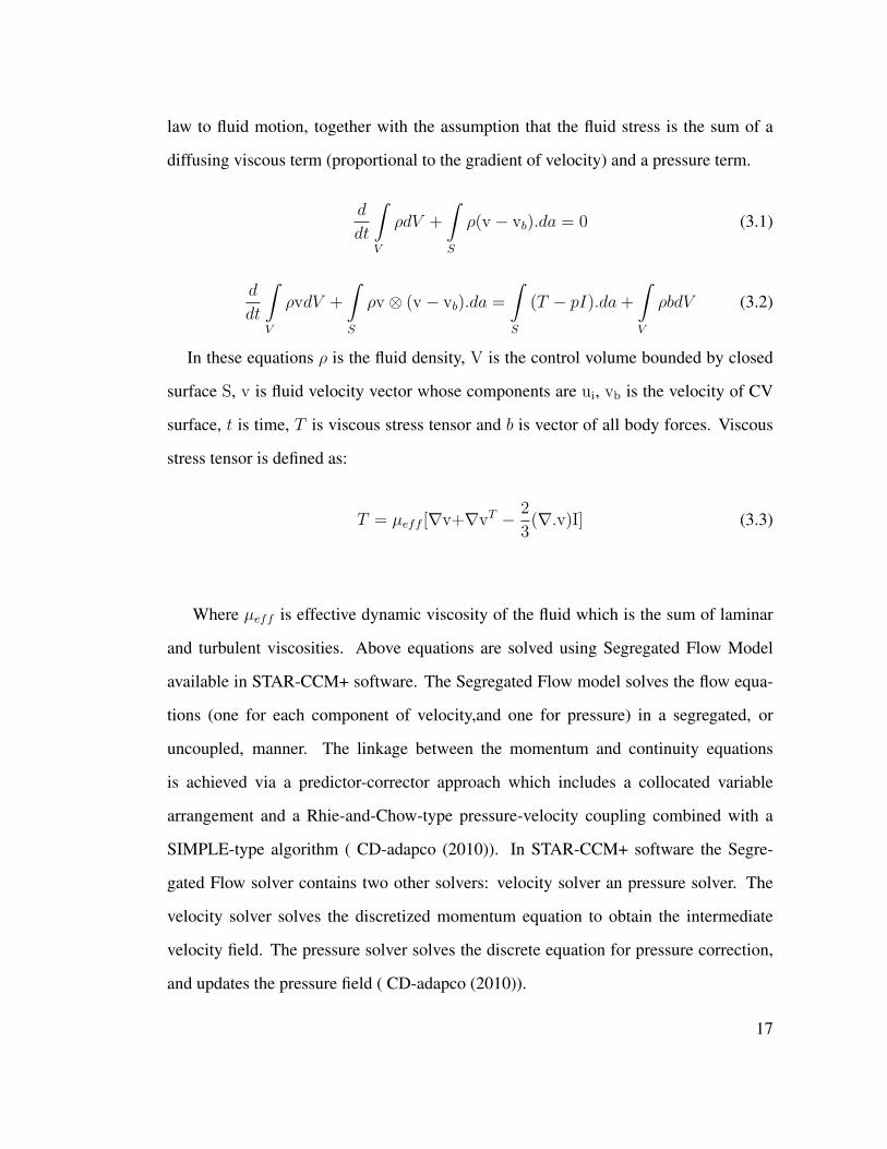
law to fluid motion, together with the assumption that the fluid stress is the sum of a
diffusing viscous term (proportional to the gradient of velocity) and a pressure term.
d
dt
∫
V
ρdV +
∫
S
ρ(v − vb).da = 0 (3.1)
d
dt
∫
V
ρvdV +
∫
S
ρv ⊗ (v − vb).da =
∫
S
(T − pI).da+
∫
V
ρbdV (3.2)
In these equations ρ is the fluid density, V is the control volume bounded by closed
surface S, v is fluid velocity vector whose components are ui, vb is the velocity of CV
surface, t is time, T is viscous stress tensor and b is vector of all body forces. Viscous
stress tensor is defined as:
T = µeff [∇v+∇vT − 2
3(∇.v)I] (3.3)
Where µeff is effective dynamic viscosity of the fluid which is the sum of laminar
and turbulent viscosities. Above equations are solved using Segregated Flow Model
available in STAR-CCM+ software. The Segregated Flow model solves the flow equa-
tions (one for each component of velocity,and one for pressure) in a segregated, or
uncoupled, manner. The linkage between the momentum and continuity equations
is achieved via a predictor-corrector approach which includes a collocated variable
arrangement and a Rhie-and-Chow-type pressure-velocity coupling combined with a
SIMPLE-type algorithm ( CD-adapco (2010)). In STAR-CCM+ software the Segre-
gated Flow solver contains two other solvers: velocity solver an pressure solver. The
velocity solver solves the discretized momentum equation to obtain the intermediate
velocity field. The pressure solver solves the discrete equation for pressure correction,
and updates the pressure field ( CD-adapco (2010)).
17
3.3 Discretization
The equations in previous section are discretized according to Finite Volume method
(FVM). In Finite Volume Method the solution domain is subdivided into a finite number
of small cells called control volumes (CVs). Usually CVs are defined by a suitable grid
and computational node is assigned to the CV center. All variations of FVM share the
same discretization principals. They are different in relations between various locations
within integration volume. The integral form of Navier Stokes equations are applied to
each CV, as well as the solution domain as a whole. Summing all the equations for all
CVs we obtain global conservation equation since surface integrals over inner CV faces
cancel out. The final result is a set of linear algebraic equations with the total number
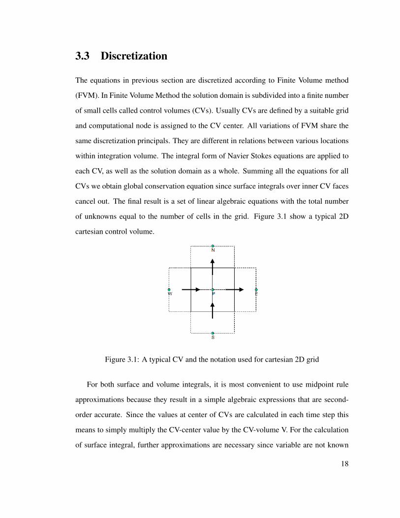
of unknowns equal to the number of cells in the grid. Figure 3.1 show a typical 2D
cartesian control volume.
Figure 3.1: A typical CV and the notation used for cartesian 2D grid
For both surface and volume integrals, it is most convenient to use midpoint rule
approximations because they result in a simple algebraic expressions that are second-
order accurate. Since the values at center of CVs are calculated in each time step this
means to simply multiply the CV-center value by the CV-volume V. For the calculation
of surface integral, further approximations are necessary since variable are not known
18
at cell-face centers. Bellow discretization schemes used to discretize continuity and
momentum equations are explained in more detail.
3.3.1 Momentum Equation in Discrete Form
Applying Equation 3.2 to a cell-centered control volume for cell-0, results in the follow-
ing discrete equation for the transport of velocity ( CD-adapco (2010)):
d
dt(ρvV )0 +
∑
f
[vρ(v − vg).a]f = −∑
f
(pI.a)f +∑
f
T.a (3.4)
The discrete equation for each velocity component may be expressed implicitly as
a linear system of equation. The transient terms, body forces and convective flux for
each velocity component is discretized based on discretization techniques explained for
transport of a simple scalar quantity in Appendix A. To evaluate the stress tensor T , the
velocity tensor gradient at the face ∇vf needs to be calculated in terms of cell velocities
according to following formula ( CD-adapco (2010)):
∇vf = ∆v ⊗ ~α + ∇vf − (∇vf .ds)⊗ ~α (3.5)
Where ∆v = v1 − v0 and ∇vf = ∇v0+∇v12
. Where ∇v0 and ∇v1 are the velocity
gradient tensors at cells 0 and 1. The vector −→α is ~α = aa.ds
. For boundary faces depend-
ing on the flow regime (turbulent vs laminar) and the type of boundary condition used,
STAR-CCM+ uses available information at the boundary to calculate stress tensor at the
face (More information can be found in ( CD-adapco (2010))).
19
3.3.2 Continuity Equation in Discrete Form
STAR-CCM+ discretizes continuity equation as follows ( CD-adapco (2010)):
∑
f
mf =∑
f
(m∗
f+m′
f ) = 0 (3.6)
In equation 3.6, m∗
f is uncorrected mass flow rate which is computed after the discrete
momentum equation have been solved according to following equation ( CD-adapco
(2010)):
m∗
f = ρf [a.(v∗0 + v∗1
2)−Gf ]− γf (3.7)
where v∗0 and v∗1 are the cell velocities after the discrete momentum equations have been
solved. Gf = (a.vg)f is the grid flux which is zero if velocity of grid vg is zero. γf is
the Rhie-and-Chow-type dissipation at the face, given by:
γf = Qf (p∗
1 − p∗0 − ∇p∗f .ds) (3.8)
where:
Qf = ρf (V0
a0+
V1
a1)−→α .a (3.9)
V0 and V1 are volumes for cell-0 and cell-1, respectively. a0 and a1 are the average of the
momentum coefficients for all components of momentum for cell 0 and 1,respectively.
p∗0 and p∗1 are the cell pressures from previous iteration. ∇p∗f is the volume-weighted
average of the cell gradients of pressure , ∇p∗0 and ∇p∗
1 . The mass flow correction m′
f
is given by the following equation ( CD-adapco (2010)):
m′
f = Qf (p′
0 − p′1) +m∗
f
ρf(∂ρ
∂p)Tp
′
upwind (3.10)
20
where p′1 and p′0 are the cell pressure corrections, and p′upwind is given by:
p′upwind =
p′0 for m∗
f > 0
p′1 for m∗
f < 0(3.11)
The discrete pressure correction equation is obtained from Equations 3.6 and 3.10 and
is written in coefficient form as:
app′
p +∑
n
anp′
n = r (3.12)
The residual r is simply the net mass flow into the cell:
r = −∑
f
m∗
f (3.13)
On the boundary faces where velocity is specified, such as walls, symmetry and inlet
boundaries, the value of m∗
f is calculated directly from known velocity v∗f on boundaries
according to the following equation ( CD-adapco (2010)).
m∗
f = ρf (a.v∗
f −Gf ) (3.14)
For pressure correction Neumann condition is used:
p′f = p′0 (3.15)
21
and the mass flux corrections are zero. For specified-pressure boundary condition, the
pressure corrections will not be zero. The uncorrected boundary mass flux is given by
following equation ( CD-adapco (2010)):
m∗
f = ρf (a.vf −Gf )− γf (3.16)
where vf is boundary velocity and γf is dissipation coefficient given as:
γf = Qf (p∗
f − p∗0 − ∇p∗0.ds) (3.17)
for subsonic outflow p′f=0, p′upwind = p′0 and equation 3.10 becomes ( CD-adapco
(2010)):
m′
f = [Qf + vf .a(∂ρ
∂p)T ]p
′
0 (3.18)
for subsonic inflow, p′upwind=0. The mass flow correction m′
f is given by ( CD-adapco
(2010)):
m′
f =vf .aQf
vf .a−Qf |vf |2(3.19)
and:
p′f =|vf |2Qf
Qf |vf |2 − vf .ap′0 (3.20)
For supersonic inflow and outflow different formulas are provided which can be found
in STAR-CCM+ manual. The discretization schemes provided above are chosen from
STAR-CCM+ manual based on relevancy to our specific problem.
3.4 SIMPLE Solver Algorithm
SIMPLE is an acronym for Semi-Implicit Method for Pressure Linked Equations. In
computational fluid dynamics (CFD), SIMPLE algorithm is a widely used iterative
22
numerical procedure to solve the Navier-Stokes equations. This method forms the
basics of many commercial CFD packages. Application of SIMPLE algorithm to Navier
Stokes equations in STAR-CCM+ includes the following steps ( CD-adapco (2010)):
1. Set the boundary conditions.
2. Compute reconstruction gradient of velocity and pressure.
3. Compute velocity and pressure gradients.
4. Solve the discretized momentum equation to create the intermediate velocity field
v∗.
5. Compute uncorrected mass fluxes at faces m∗
f
6. Solve pressure correction equation to produce cell values of the pressure correc-
tion p′.
7. Update pressure field pn+1 = pn + ωp′ where ω is under relaxation factor for
pressure.
8. Update boundary pressure correction p′b
9. Correct face mass fluxes mn+1f = m∗
f + m′
f
10. Correct cell velocities where ∇p′ is gradient of the pressure corrections, avp is
vector of central coefficients for discretized linear system representing the velocity
equation and V is cell volume.
vn+1 = v∗ − V∇p′
avp(3.21)
11. Update density due to pressure changes.
23
12. Free all temporary storage.
STAR-CCM+ uses specific methods to calculate velocity and pressure gradients used
in discretized continuity and momentum equations. These methods are explained in
appendix A for a simple scaler φ.
3.5 Numerical Method for Solving Algebraic Equations
Application of finite volume discretization schemes described in previous sections to
Navier Stokes equations will result in the coefficients of linear equation system that
needs to be solved implicitly. The algebraic system for transported variable φ at a typical
point p at iteration k+1 is written as ( CD-adapco (2010)):
apφk+1p +
∑
n
anφk+1n = b (3.22)
where the summation is over all neighbor n of cell p. The right hand side b is evaluated
from previous iteration and coefficients ap and an are obtained directly from discretized
equations. Allowing φk+1p to change too much can cause instability, so we implicitly
introduce ω to cut out steep oscillations. Equation 3.22 becomes ( CD-adapco (2010)):
apωφk+1p +
∑
n
anφk+1n = b+
apω(1− ω)φk
p (3.23)
where k+1 implies the values after the solution is produced and source term at right
hand side is evaluated at the previous iteration k. Rather than solving equation 3.23 for
φk+1p it is more convenient to cast into delta form defining ∆φp = φk+1
p − φkp. System to
be solved becomes ( CD-adapco (2010)):
apω∆φp +
∑
n
an∆φn = b− apφkp −
∑
n
anφkn (3.24)
24
The right hand side r = b − apφkp −
∑
n
anφkn is termed the residual, and represents the
discretized form of original transport equation at iteration k. The residual will be zero
when the discretized equation is satisfied exactly.
System of equations arising from most realistic CFD problems are usually very large
and contain several million equations. How ever these systems are usually sparse (have
many zero entries). Any valid procedure can be used to solve these algebraic equations.
How ever even with the latest advances in computer hardware technology, computa-
tional resources are still a major constraint. There are two family of solution techniques
for linear algebraic equations: direct methods and indirect or iterative methods. Simple
examples of direct methods are Cramer’s rule matrix inversion and Gaussian elimina-
tion. Iterative methods are based on the repeated application of a relatively simple algo-
rithm leading to eventual conversion after a sometimes large number of repetitions. Well
known examples are Jacobi and Gauss-Seidel methods. The total number of iterations
can not be predicted in advance and the convergence is not guarantee unless the system
of equations satisfies fairly exact criteria. Iterative methods are usually far more effi-
cient than direct methods for large equation sets. In addition Jacobi and Gauss-Seidel
methods which are general purpose point iterative algorithms are easily implementable.
The only problem with these iterative procedures is their convergence rate which can be
really slow when the system of equations is large. Recently, multigrid acceleration tech-
niques have been developed that have improved the convergence rate of iterative solvers
to such an extent that they are now the method of choice in commercial CFD codes.
Moreover, the SIMPLE algorithm for coupling of continuity and momentum equations
is itself iterative. Hence, there is no need to obtain a very accurate intermediate solutions
as long as the iteration process eventually converges to the true solution.
25
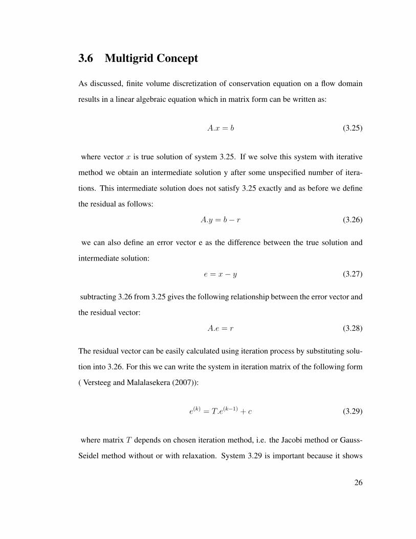
3.6 Multigrid Concept
As discussed, finite volume discretization of conservation equation on a flow domain
results in a linear algebraic equation which in matrix form can be written as:
A.x = b (3.25)
where vector x is true solution of system 3.25. If we solve this system with iterative
method we obtain an intermediate solution y after some unspecified number of itera-
tions. This intermediate solution does not satisfy 3.25 exactly and as before we define
the residual as follows:
A.y = b− r (3.26)
we can also define an error vector e as the difference between the true solution and
intermediate solution:
e = x− y (3.27)
subtracting 3.26 from 3.25 gives the following relationship between the error vector and
the residual vector:
A.e = r (3.28)
The residual vector can be easily calculated using iteration process by substituting solu-
tion into 3.26. For this we can write the system in iteration matrix of the following form
( Versteeg and Malalasekera (2007)):
e(k) = T.e(k−1) + c (3.29)
where matrix T depends on chosen iteration method, i.e. the Jacobi method or Gauss-
Seidel method without or with relaxation. System 3.29 is important because it shows
26
how the error propagates from one iteration to the next. It also highlights the crucial role
played by the iteration matrix. The properties of iteration matrix T determine the rate of
error propagation and hence the rate of convergence. These properties have been studied
extensively along with the mathematical properties of the error propagation as a function
of iterative technique, mesh size, discretization scheme etc. It has been established that
the solution error has components with the range of wave lengths that are multiples
of mesh size. Iteration methods cause rapid reduction of error components with short
wave lengths up to a few multiples of the mesh size . How ever long wave length
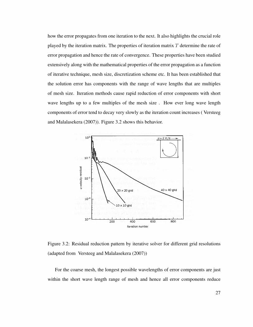
components of error tend to decay very slowly as the iteration count increases ( Versteeg
and Malalasekera (2007)). Figure 3.2 shows this behavior.
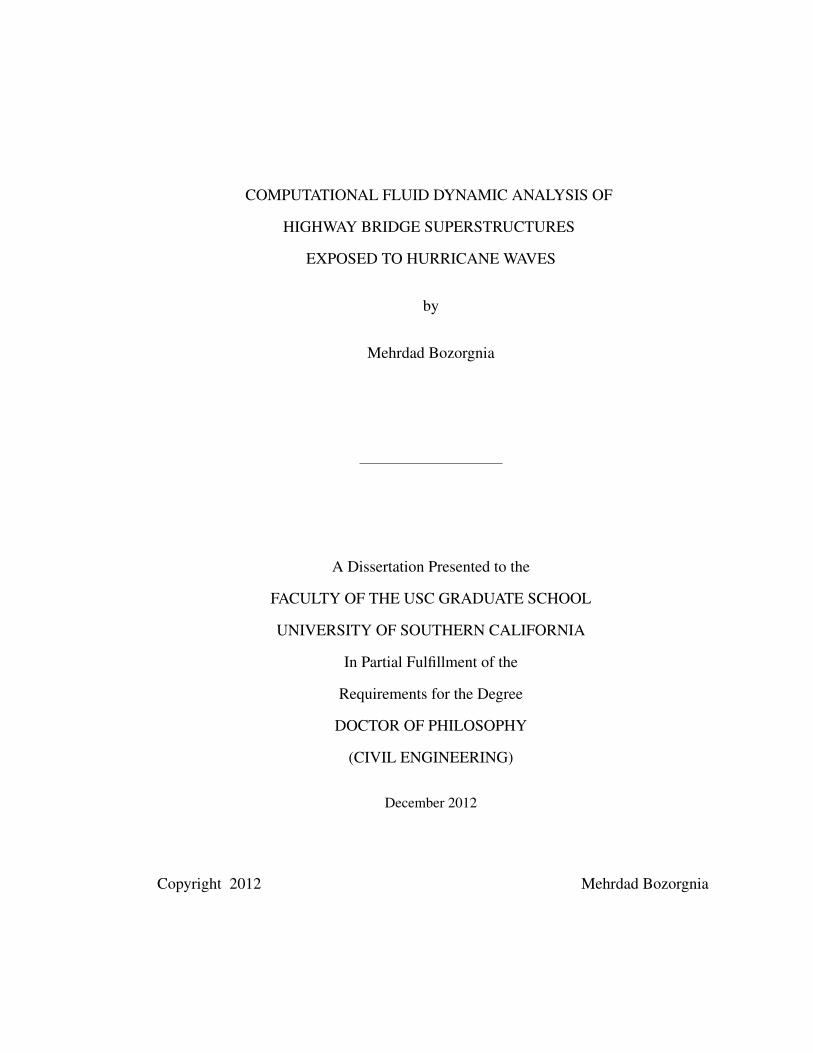
7.7 MULTIGRID TECHNIQUES 229
Multigrid .
tech iques We have established in earlier chapters that the discretisation error reduces
with the mesh spacing. In other words, the finer the mesh, the better the
accuracy of a CFD simulation. Iterative techniques are preferred over direct
methods_becuse their storage overheads are lower, which makes them more
iior the soffiiiflarge systems
fiuiThëshEMeover, we have seen in Chapt6thafThSIMPLEcontinuity and momentum gptons is itself
iëiTiVEiIênce, the i hEdiöb1in very accurate intermediate solu
iiñs long as the• iteration. process eventually converges to the true
solution. Unfortunately, it transpires that the convergence rate of iterative
methods, such. as the Jacobi and Gauss—Seidel, rapidly reduces as the
mesh is. refined.To examine the relationship between the convergence rate of an iterative
method and the number of grid cells in a problem we consider a simple
two-dimensional cavity-driven flow. The inset of Figure 7.5 shows that the
computational domain is a square cavity with a size of 1 cm x 1 cm. The lid
of the cavity is moving with a velocity of 2 rn/s in the positive x-direction.
The fluid in thecavity is air and the flow is assumed to be laminar. We use a
line—by—line iterative solver to compute the solution on three different grids
with lOx 1.Q, 20 x 20 and 40.x 40 cells.
To obtaina measure of the closeness to the true solution of an intermedi
ate solution in an iteration sequence we use the residual defined in (7.26) for
the ith equation. The average residual F over all n equations in the system
(i.e. an average over all the control volumes in the computational domain
of a ‘flow problem) is a useful indicator of iterative convergence for a given
problem:
(7.30)
j1
If the iteration process is convergent the average residual F should tend to
zero, since all contributing residuals r —> 0 as k —> oo• The average residual
B Residual reduction 100
a line—by—lineoIvcr using different
Iuiions101
Cu
U)U)
100
U)>
iO-
io400
Iteration number
Figure 3.2: Residual reduction pattern by iterative solver for different grid resolutions
(adapted from Versteeg and Malalasekera (2007))
For the coarse mesh, the longest possible wavelengths of error components are just
within the short wave length range of mesh and hence all error components reduce
27
rapidly. On the finer meshes, how ever, the longest error wave lengths can not be elimi-
nated as they fall outside the short-wave length range for which decay is rapid. Multigrid
methods are designed to exploit these inherent differences of the error behavior and use
iteration on meshes of different size. The short wavelength errors are effectively reduced
on the finest meshes, whereas the long wavelength errors decrease rapidly on the coars-
est meshes. More over the computational cost of iterations is larger on finer meshes than
on coarse meshes, so the extra cost due to iterations on the coarse meshes is offset by
the benefit of much improved convergence rate ( Versteeg and Malalasekera (2007)).
In general we have two types of Multigrid algorithms: geometric and algebraic.
Geometric multigrid uses grid geometry and the discrete equation at the coarse level
to arrive at the linear system to be solved on that level. Algebraic multigrid derives
a course level system without reference to the underlying grid geometry or discrete
equations. The coarse-grid equations are derived from arithmetic combinations of the
fine-grid coefficients. Multigrid procedure involves the following steps:
• Agglomerate cells to form coarse grid levels.
• Transfer the residual from a fine level to a a coarser level (known as restriction).
• Transfer the correction from a coarse level back to a finer level (known as prolon-
gation).
since its not always easy to get suitable discrete equations on the coarse grid using
geometric multigrid techniques, algebraic multigrid (AMG) is clearly at an advantage.
Therefore, it is used for the solution of all linear systems in the present thesis. AMG
solver in STAR-CCM+ has two cycling strategies: fixed and flexible. Fixed cycling
strategy includes recursive application of a single cycle which in STAR-CCM+ software
includes the following steps ( CD-adapco (2010)):
• (Pre)smooth
28
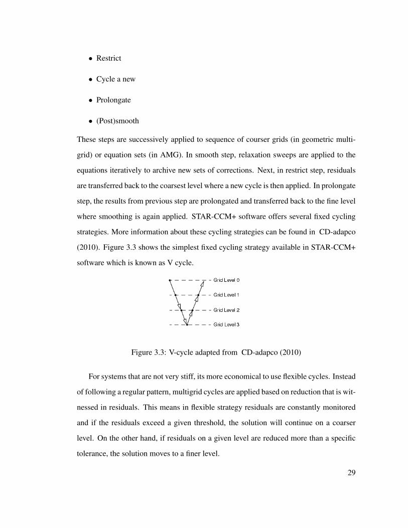
• Restrict
• Cycle a new
• Prolongate
• (Post)smooth
These steps are successively applied to sequence of courser grids (in geometric multi-
grid) or equation sets (in AMG). In smooth step, relaxation sweeps are applied to the
equations iteratively to archive new sets of corrections. Next, in restrict step, residuals
are transferred back to the coarsest level where a new cycle is then applied. In prolongate
step, the results from previous step are prolongated and transferred back to the fine level
where smoothing is again applied. STAR-CCM+ software offers several fixed cycling
strategies. More information about these cycling strategies can be found in CD-adapco
(2010). Figure 3.3 shows the simplest fixed cycling strategy available in STAR-CCM+
software which is known as V cycle.
Figure 3.3: V-cycle adapted from CD-adapco (2010)
For systems that are not very stiff, its more economical to use flexible cycles. Instead
of following a regular pattern, multigrid cycles are applied based on reduction that is wit-
nessed in residuals. This means in flexible strategy residuals are constantly monitored
and if the residuals exceed a given threshold, the solution will continue on a coarser
level. On the other hand, if residuals on a given level are reduced more than a specific
tolerance, the solution moves to a finer level.
29
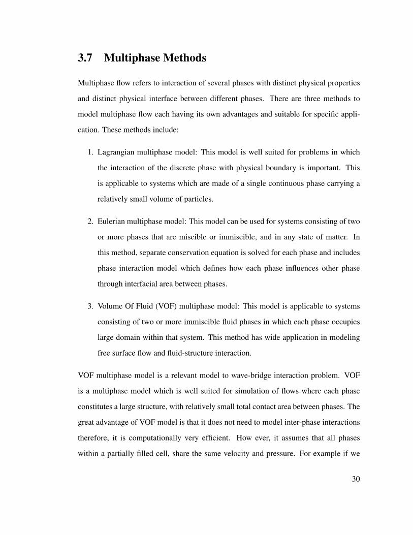
3.7 Multiphase Methods
Multiphase flow refers to interaction of several phases with distinct physical properties
and distinct physical interface between different phases. There are three methods to
model multiphase flow each having its own advantages and suitable for specific appli-
cation. These methods include:
1. Lagrangian multiphase model: This model is well suited for problems in which
the interaction of the discrete phase with physical boundary is important. This
is applicable to systems which are made of a single continuous phase carrying a
relatively small volume of particles.
2. Eulerian multiphase model: This model can be used for systems consisting of two
or more phases that are miscible or immiscible, and in any state of matter. In
this method, separate conservation equation is solved for each phase and includes
phase interaction model which defines how each phase influences other phase
through interfacial area between phases.
3. Volume Of Fluid (VOF) multiphase model: This model is applicable to systems
consisting of two or more immiscible fluid phases in which each phase occupies
large domain within that system. This method has wide application in modeling
free surface flow and fluid-structure interaction.
VOF multiphase model is a relevant model to wave-bridge interaction problem. VOF
is a multiphase model which is well suited for simulation of flows where each phase
constitutes a large structure, with relatively small total contact area between phases. The
great advantage of VOF model is that it does not need to model inter-phase interactions
therefore, it is computationally very efficient. How ever, it assumes that all phases
within a partially filled cell, share the same velocity and pressure. For example if we
30
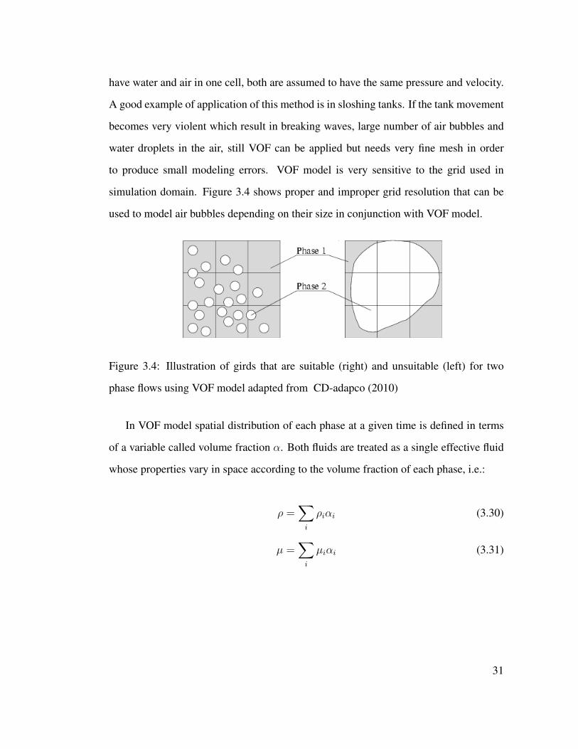
have water and air in one cell, both are assumed to have the same pressure and velocity.
A good example of application of this method is in sloshing tanks. If the tank movement
becomes very violent which result in breaking waves, large number of air bubbles and
water droplets in the air, still VOF can be applied but needs very fine mesh in order
to produce small modeling errors. VOF model is very sensitive to the grid used in
simulation domain. Figure 3.4 shows proper and improper grid resolution that can be
used to model air bubbles depending on their size in conjunction with VOF model.
Figure 3.4: Illustration of girds that are suitable (right) and unsuitable (left) for two
phase flows using VOF model adapted from CD-adapco (2010)
In VOF model spatial distribution of each phase at a given time is defined in terms
of a variable called volume fraction α. Both fluids are treated as a single effective fluid
whose properties vary in space according to the volume fraction of each phase, i.e.:
ρ =∑
i
ρiαi (3.30)
µ =∑
i
µiαi (3.31)
31
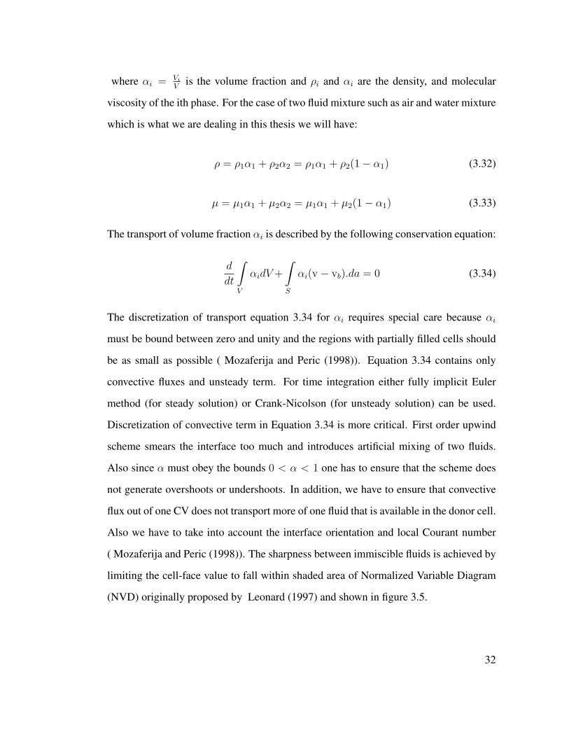
where αi = Vi
Vis the volume fraction and ρi and αi are the density, and molecular
viscosity of the ith phase. For the case of two fluid mixture such as air and water mixture
which is what we are dealing in this thesis we will have:
ρ = ρ1α1 + ρ2α2 = ρ1α1 + ρ2(1− α1) (3.32)
µ = µ1α1 + µ2α2 = µ1α1 + µ2(1− α1) (3.33)
The transport of volume fraction αi is described by the following conservation equation:
d
dt
∫
V
αidV+
∫
S
αi(v − vb).da = 0 (3.34)
The discretization of transport equation 3.34 for αi requires special care because αi
must be bound between zero and unity and the regions with partially filled cells should
be as small as possible ( Mozaferija and Peric (1998)). Equation 3.34 contains only
convective fluxes and unsteady term. For time integration either fully implicit Euler
method (for steady solution) or Crank-Nicolson (for unsteady solution) can be used.
Discretization of convective term in Equation 3.34 is more critical. First order upwind
scheme smears the interface too much and introduces artificial mixing of two fluids.
Also since α must obey the bounds 0 < α < 1 one has to ensure that the scheme does
not generate overshoots or undershoots. In addition, we have to ensure that convective
flux out of one CV does not transport more of one fluid that is available in the donor cell.
Also we have to take into account the interface orientation and local Courant number
( Mozaferija and Peric (1998)). The sharpness between immiscible fluids is achieved by
limiting the cell-face value to fall within shaded area of Normalized Variable Diagram
(NVD) originally proposed by Leonard (1997) and shown in figure 3.5.
32
Figure 3.5: Upwind, downwind and central cells used in the analysis (left) and con-
vection boundedness criterion in the NVD diagram (right) adapted from CD-adapco
(2010)
More details about these methods can be found in ( Mozaferija and Peric (1998)) and
( CD-adapco (2010)). Figure 3.6 shows how free surface is constructed from volume
fraction α using VOF multiphase model.
Figure 3.6: a)True interface b)Volume Fraction
33
Chapter 4
MODEL VALIDATION FOR UPLIFT
FORCES ON FLAT PLATE
4.1 Solitary Wave
Before applying CFD software STAR-CCM+ to the wave-bridge interaction problem,
the software is validated for the problem of a solitary wave interacting with a simple flat
plate. Solitary wave is a relevant model of an ocean wave in shoal water. John Scott
Russell in 1834 was the first to report on the wave, while conducting experiments to
determine the most efficient design for canal boats. That is why, in fluid dynamics the
wave is now called a Scott Russell solitary wave or soliton ( Wikipedia (2012)).
There are several theoretical solutions of the solitary wave equations which are often
referred to in literature. Boussinesq (1872) obtained an analytical solution for wave
profile, wave propagation speed, and the water particle velocities. McCowan (1891)
carried out the solution to the first order approximation and determined the wave pro-
file, wave speed, fluid particle velocities, and an estimate of the limiting height of wave.
Laitone (1963) obtained a solution similar to that of Boussinesq, but his solution con-
tained higher order terms. Grimshaw (1970) proposed a third order solitary wave the-
ory through a series expansions in terms of the relative wave amplitude. Fenton (1972)
obtained a ninth order solution for the solitary wave. In his analysis, a form of solution
was first assumed and then, coefficients were obtained numerically. Although Laitone
(1963), Grimshaw (1970), and Fenton (1972) solitary wave theories are derived from
34
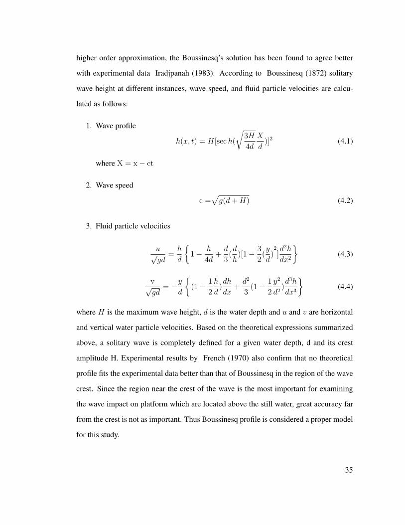
higher order approximation, the Boussinesq’s solution has been found to agree better
with experimental data Iradjpanah (1983). According to Boussinesq (1872) solitary
wave height at different instances, wave speed, and fluid particle velocities are calcu-
lated as follows:
1. Wave profile
h(x, t) = H[sech(
√
3H
4d
X
d)]2 (4.1)
where X = x− ct
2. Wave speed
c =√
g(d+H) (4.2)
3. Fluid particle velocities
u√gd
=h
d
{
1− h
4d+
d
3(d
h)[1− 3
2(y
d)2
]d2h
dx2
}
(4.3)
v√gd
= −y
d
{
(1− 1
2
h
d)dh
dx+
d2
3(1− 1
2
y2
d2)d3h
dx3
}
(4.4)
where H is the maximum wave height, d is the water depth and u and v are horizontal
and vertical water particle velocities. Based on the theoretical expressions summarized
above, a solitary wave is completely defined for a given water depth, d and its crest
amplitude H. Experimental results by French (1970) also confirm that no theoretical
profile fits the experimental data better than that of Boussinesq in the region of the wave
crest. Since the region near the crest of the wave is the most important for examining
the wave impact on platform which are located above the still water, great accuracy far
from the crest is not as important. Thus Boussinesq profile is considered a proper model
for this study.
35
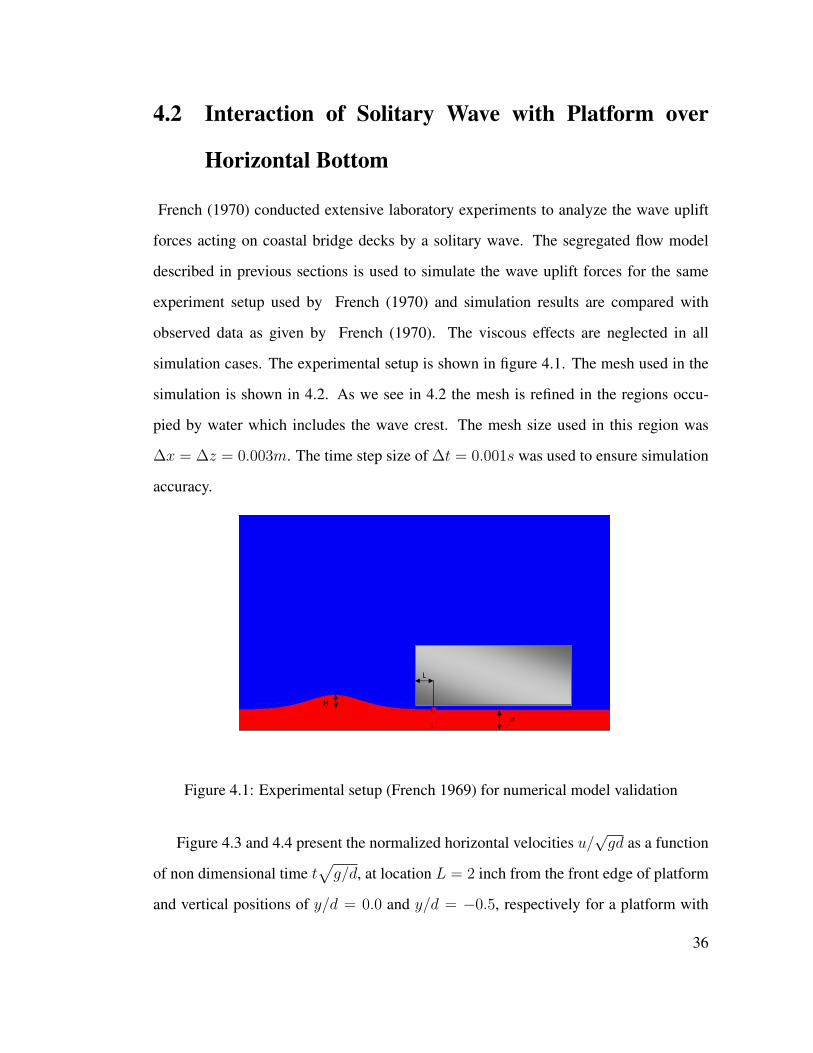
4.2 Interaction of Solitary Wave with Platform over
Horizontal Bottom
French (1970) conducted extensive laboratory experiments to analyze the wave uplift
forces acting on coastal bridge decks by a solitary wave. The segregated flow model
described in previous sections is used to simulate the wave uplift forces for the same
experiment setup used by French (1970) and simulation results are compared with
observed data as given by French (1970). The viscous effects are neglected in all
simulation cases. The experimental setup is shown in figure 4.1. The mesh used in the
simulation is shown in 4.2. As we see in 4.2 the mesh is refined in the regions occu-
pied by water which includes the wave crest. The mesh size used in this region was
∆x = ∆z = 0.003m. The time step size of ∆t = 0.001s was used to ensure simulation
accuracy.
H
L
d
Figure 4.1: Experimental setup (French 1969) for numerical model validation
Figure 4.3 and 4.4 present the normalized horizontal velocities u/√gd as a function
of non dimensional time t√
g/d, at location L = 2 inch from the front edge of platform
and vertical positions of y/d = 0.0 and y/d = −0.5, respectively for a platform with
36
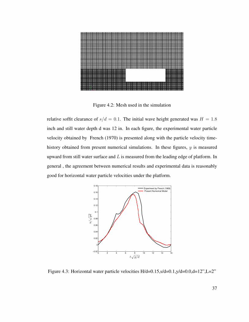
Figure 4.2: Mesh used in the simulation
relative soffit clearance of s/d = 0.1. The initial wave height generated was H = 1.8
inch and still water depth d was 12 in. In each figure, the experimental water particle
velocity obtained by French (1970) is presented along with the particle velocity time-
history obtained from present numerical simulations. In these figures, y is measured
upward from still water surface and L is measured from the leading edge of platform. In
general , the agreement between numerical results and experimental data is reasonably
good for horizontal water particle velocities under the platform.
0 2 4 6 8 10 12 14 16−0.02
0
0.02
0.04
0.06
0.08
0.1
0.12
0.14
0.16
0.18
t√
g/d
u/√
gd
Experiment by French (1969)
Present Numerical Model
Figure 4.3: Horizontal water particle velocities H/d=0.15,s/d=0.1,y/d=0.0,d=12”,L=2”
37
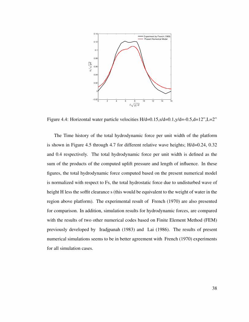
0 2 4 6 8 10 12 14 16−0.02
0
0.02
0.04
0.06
0.08
0.1
0.12
0.14
t√
g/d
u/√
gd
Experiment by French (1969)
Present Numerical Model
Figure 4.4: Horizontal water particle velocities H/d=0.15,s/d=0.1,y/d=-0.5,d=12”,L=2”
The Time history of the total hydrodynamic force per unit width of the platform
is shown in Figure 4.5 through 4.7 for different relative wave heights; H/d=0.24, 0.32
and 0.4 respectively. The total hydrodynamic force per unit width is defined as the
sum of the products of the computed uplift pressure and length of influence. In these
figures, the total hydrodynamic force computed based on the present numerical model
is normalized with respect to Fs, the total hydrostatic force due to undisturbed wave of
height H less the soffit clearance s (this would be equivalent to the weight of water in the
region above platform). The experimental result of French (1970) are also presented
for comparison. In addition, simulation results for hydrodynamic forces, are compared
with the results of two other numerical codes based on Finite Element Method (FEM)
previously developed by Iradjpanah (1983) and Lai (1986). The results of present
numerical simulations seems to be in better agreement with French (1970) experiments
for all simulation cases.
38
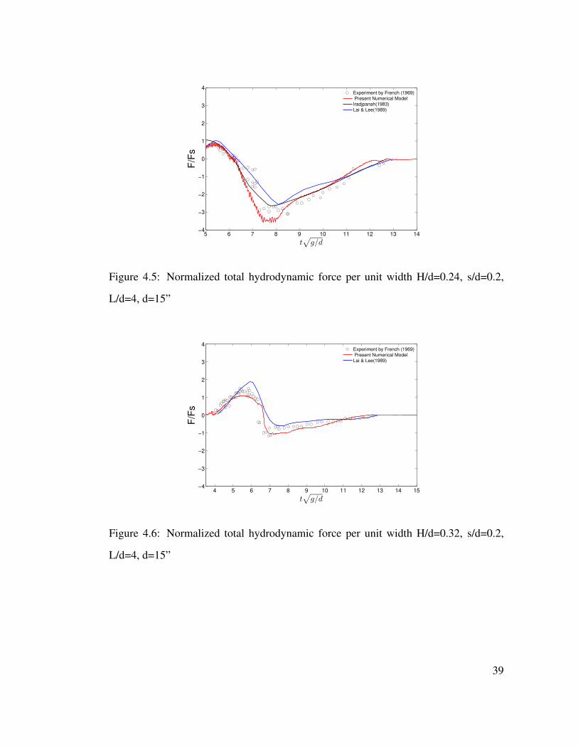
5 6 7 8 9 10 11 12 13 14−4
−3
−2
−1
0
1
2
3
4
t√
g/d
F/F
s
Experiment by French (1969)
Present Numerical Model
Iradjpanah(1983)
Lai & Lee(1989)
Figure 4.5: Normalized total hydrodynamic force per unit width H/d=0.24, s/d=0.2,
L/d=4, d=15”
4 5 6 7 8 9 10 11 12 13 14 15−4
−3
−2
−1
0
1
2
3
4
t√
g/d
F/F
s
Experiment by French (1969)
Present Numerical Model
Lai & Lee(1989)
Figure 4.6: Normalized total hydrodynamic force per unit width H/d=0.32, s/d=0.2,
L/d=4, d=15”
39
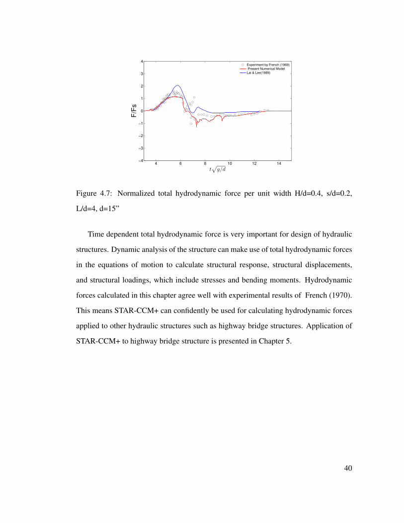
4 6 8 10 12 14−4
−3
−2
−1
0
1
2
3
4
t√
g/d
F/F
s
Experiment by French (1969)
Present Numerical Model
Lai & Lee(1989)
Figure 4.7: Normalized total hydrodynamic force per unit width H/d=0.4, s/d=0.2,
L/d=4, d=15”
Time dependent total hydrodynamic force is very important for design of hydraulic
structures. Dynamic analysis of the structure can make use of total hydrodynamic forces
in the equations of motion to calculate structural response, structural displacements,
and structural loadings, which include stresses and bending moments. Hydrodynamic
forces calculated in this chapter agree well with experimental results of French (1970).
This means STAR-CCM+ can confidently be used for calculating hydrodynamic forces
applied to other hydraulic structures such as highway bridge structures. Application of
STAR-CCM+ to highway bridge structure is presented in Chapter 5.
40
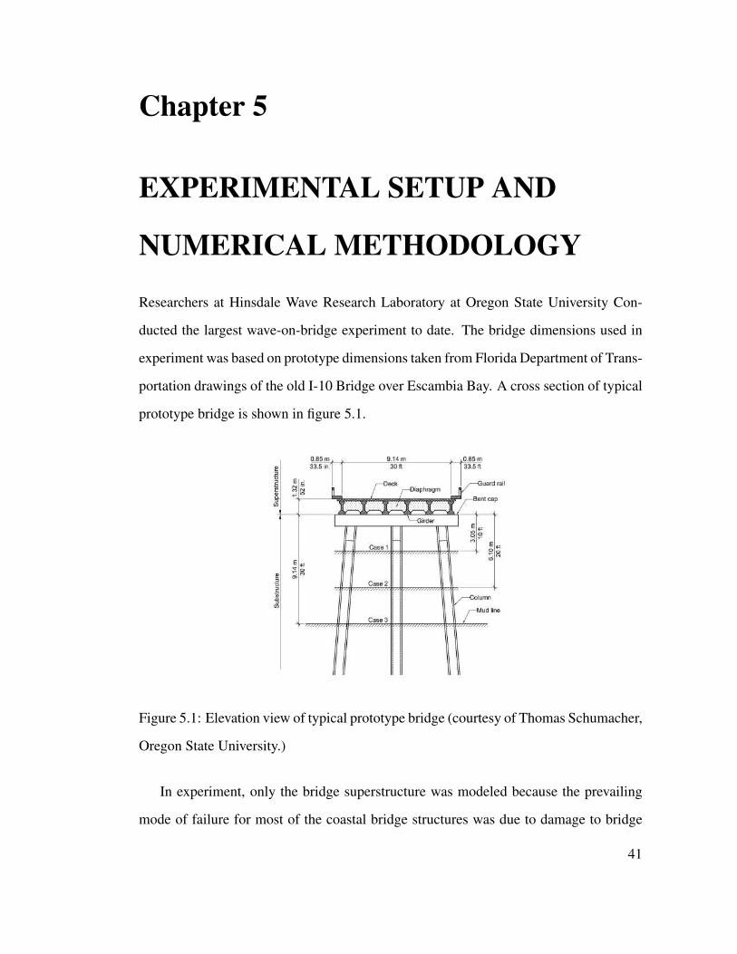
Chapter 5
EXPERIMENTAL SETUP AND
NUMERICAL METHODOLOGY
Researchers at Hinsdale Wave Research Laboratory at Oregon State University Con-
ducted the largest wave-on-bridge experiment to date. The bridge dimensions used in
experiment was based on prototype dimensions taken from Florida Department of Trans-
portation drawings of the old I-10 Bridge over Escambia Bay. A cross section of typical
prototype bridge is shown in figure 5.1.
Figure 5.1: Elevation view of typical prototype bridge (courtesy of Thomas Schumacher,
Oregon State University.)
In experiment, only the bridge superstructure was modeled because the prevailing
mode of failure for most of the coastal bridge structures was due to damage to bridge
41
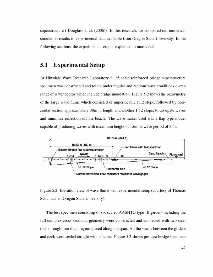
superstructure ( Douglass et al. (2006)). In this research, we compared our numerical
simulation results to experimental data available from Oregon State University. In the
following sections, the experimental setup is explained in more detail.
5.1 Experimental Setup
At Hinsdale Wave Research Laboratory a 1:5 scale reinforced bridge superstructure
specimen was constructed and tested under regular and random wave conditions over a
range of water depths which include bridge inundation. Figure 5.2 shows the bathymetry
of the large wave flume which consisted of impermeable 1:12 slope, followed by hori-
zontal section approximately 30m in length and another 1:12 slope, to dissipate waves
and minimize reflection off the beach. The wave maker used was a flap-type model
capable of producing waves with maximum height of 1.6m at wave period of 3.5s.
Figure 5.2: Elevation view of wave flume with experimental setup (courtesy of Thomas
Schumacher, Oregon State University).
The test specimen consisting of six scaled AASHTO type III girders including the
full complex cross-sectional geometry were constructed and connected with two steel
rods through four diaphragms spaced along the span. All the seams between the girders
and deck were sealed airtight with silicone. Figure 5.3 shows pre-cast bridge specimen
42
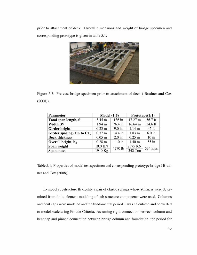
prior to attachment of deck. Overall dimensions and weight of bridge specimen and
corresponding prototype is given in table 5.1.
Figure 5.3: Pre-cast bridge specimen prior to attachment of deck ( Bradner and Cox
(2008)).
Parameter Model (1:5) Prototype(1:1)
Total span length, S 3.45 m 136 in 17.27 m 56.7 ft
Width ,W 1.94 m 76.4 in 16.64 m 54.6 ft
Girder height 0.23 m 9.0 in 1.14 m 45 ft
Girder spacing (CL to CL) 0.37 m 14.4 in 1.83 m 6.0 in
Deck thickness 0.05 m 2.0 in 0.25 m 10 in
Overall height, hd 0.28 m 11.0 in 1.40 m 55 in
Span weight 19.0 KN 4270 lb
2375 KN 534 kips
Span mass 1940 Kg 242 Ton
Table 5.1: Properties of model test specimen and corresponding prototype bridge ( Brad-
ner and Cox (2008))
To model substructure flexibility a pair of elastic springs whose stiffness were deter-
mined from finite element modeling of sub structure components were used. Columns
and bent caps were modeled and the fundamental period T was calculated and converted
to model scale using Froude Criteria. Assuming rigid connection between column and
bent cap and pinned connection between bridge column and foundation, the period for
43
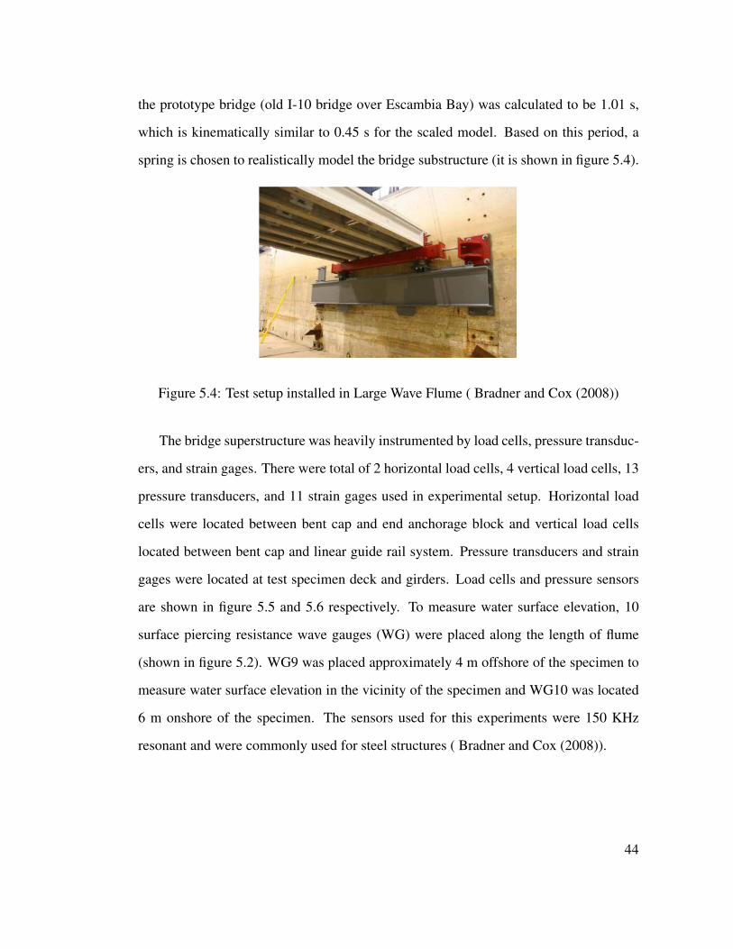
the prototype bridge (old I-10 bridge over Escambia Bay) was calculated to be 1.01 s,
which is kinematically similar to 0.45 s for the scaled model. Based on this period, a
spring is chosen to realistically model the bridge substructure (it is shown in figure 5.4).
Figure 5.4: Test setup installed in Large Wave Flume ( Bradner and Cox (2008))
The bridge superstructure was heavily instrumented by load cells, pressure transduc-
ers, and strain gages. There were total of 2 horizontal load cells, 4 vertical load cells, 13
pressure transducers, and 11 strain gages used in experimental setup. Horizontal load
cells were located between bent cap and end anchorage block and vertical load cells
located between bent cap and linear guide rail system. Pressure transducers and strain
gages were located at test specimen deck and girders. Load cells and pressure sensors
are shown in figure 5.5 and 5.6 respectively. To measure water surface elevation, 10
surface piercing resistance wave gauges (WG) were placed along the length of flume
(shown in figure 5.2). WG9 was placed approximately 4 m offshore of the specimen to
measure water surface elevation in the vicinity of the specimen and WG10 was located
6 m onshore of the specimen. The sensors used for this experiments were 150 KHz
resonant and were commonly used for steel structures ( Bradner and Cox (2008)).
44
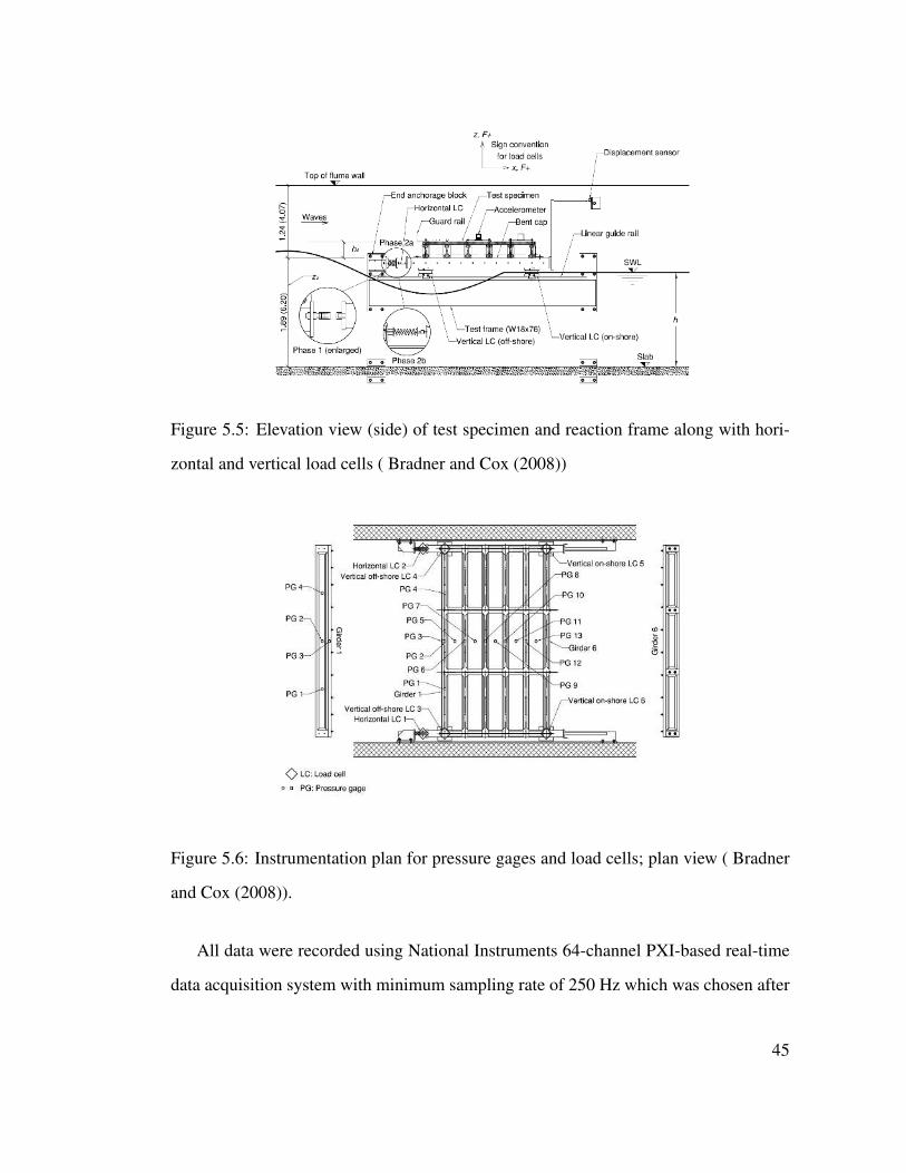
Figure 5.5: Elevation view (side) of test specimen and reaction frame along with hori-
zontal and vertical load cells ( Bradner and Cox (2008))
Figure 3-10. Instrumentation plan for pressure gages and load cells; plan view (deck not
Figure 5.6: Instrumentation plan for pressure gages and load cells; plan view ( Bradner
and Cox (2008)).
All data were recorded using National Instruments 64-channel PXI-based real-time
data acquisition system with minimum sampling rate of 250 Hz which was chosen after
45

finding little variation in the data among test trials which were sampled at higher rates
( Bradner and Cox (2008)).
Wave heights and corresponding forces used in the analysis were taken from a win-
dow of time between the first wave striking the specimen and the observation of re-
reflected waves in the incident wave data. The length of this window varied with wave
celerity, and had an average of approximately 27 seconds. The number of waves and
corresponding forces within this window ranged between 5 and 16 with an average of
8.3. Wave heights for different trials were calculated by taking the mean of the wave
heights within this window. A photo of the tank condition during a typical wave trial is
shown in figure 5.7.
Figure 5.7: Photo of the bridge specimen during wave trial ( Bradner and Cox (2008)).
Forces are measured using six load cells (LCs) shown in figure 5.5. Total vertical
force is calculated by adding data from load cells 3, 4, 5, and 6 (LC3, LC4, LC5, LC6).
Horizontal forces are calculated by adding data from load cells 1 and 2 (LC1, LC2).
Load cell data was zeroed out at the beginning of each trial, and as a results buoyancy
forces due to a change of SWL are eliminated from load cell measurement. Figure
5.8 and 5.9 shows time series of total horizontal and vertical forces applied to bridge
superstructure for wave trial of 1325 with wave height of H = 0.5m and wave period of
46
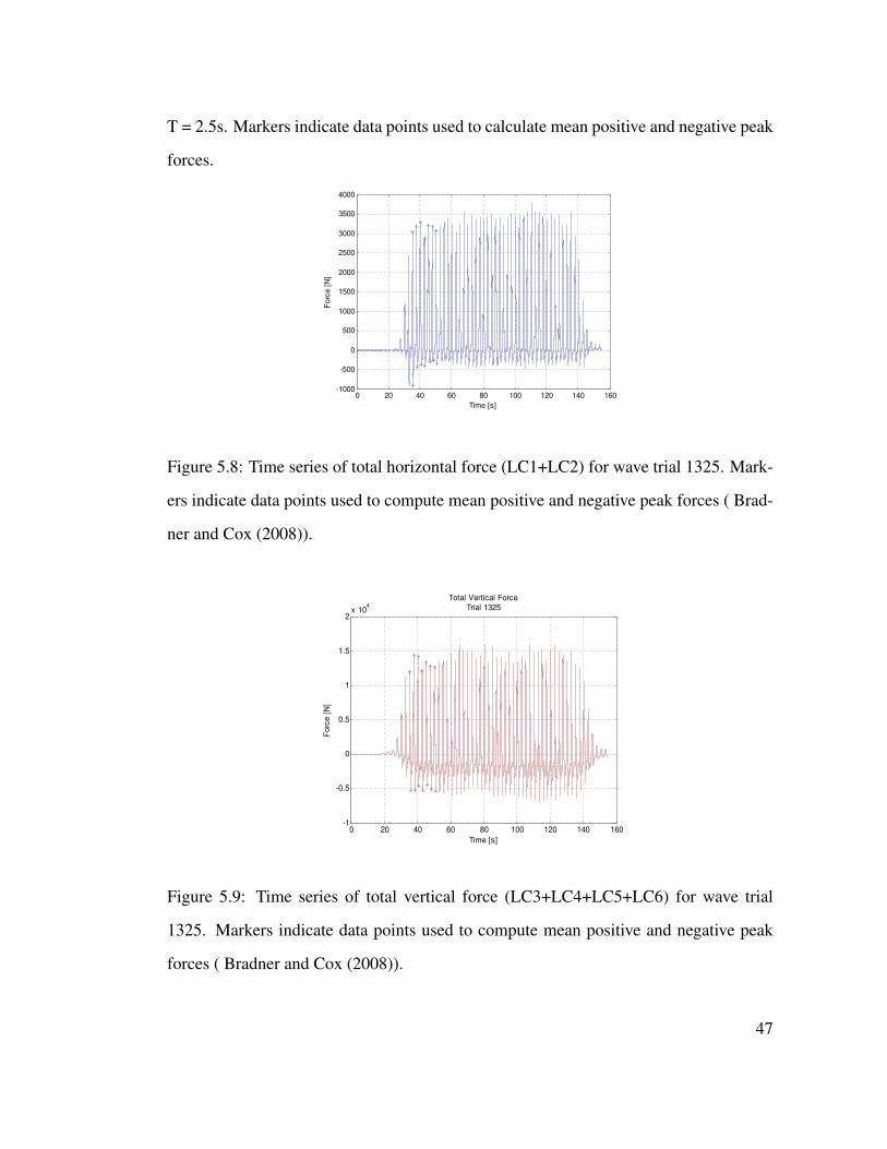
T = 2.5s. Markers indicate data points used to calculate mean positive and negative peak
forces.
Figure 4-10. Time series of total horizontal force (LC1 + LC2) for regular wave trial 1325.
0 20 40 60 80 100 120 140 160-1000
-500
0
500
1000
1500
2000
2500
3000
3500
4000
Time [s]
Forc
e [
N]
Figure 5.8: Time series of total horizontal force (LC1+LC2) for wave trial 1325. Mark-
ers indicate data points used to compute mean positive and negative peak forces ( Brad-
ner and Cox (2008)).
0 20 40 60 80 100 120 140 160-1
-0.5
0
0.5
1
1.5
2x 10
4
Total Vertical Force
Trial 1325
Time [s]
Forc
e [
N]
Figure 5.9: Time series of total vertical force (LC3+LC4+LC5+LC6) for wave trial
1325. Markers indicate data points used to compute mean positive and negative peak
forces ( Bradner and Cox (2008)).
47
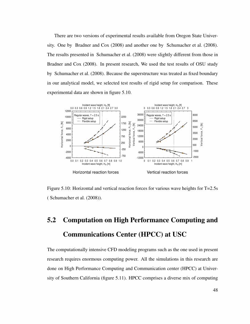
There are two versions of experimental results available from Oregon State Univer-
sity. One by Bradner and Cox (2008) and another one by Schumacher et al. (2008).
The results presented in Schumacher et al. (2008) were slightly different from those in
Bradner and Cox (2008). In present research, We used the test results of OSU study
by Schumacher et al. (2008). Because the superstructure was treated as fixed boundary
in our analytical model, we selected test results of rigid setup for comparison. These
experimental data are shown in figure 5.10.
Incident wave height, Hin [m]
Incident wave height, Hin [ft]
Ho
riz
on
tal
forc
e,
Fh
[N]
Ho
riz
on
tal
forc
e,
Fh
[lb
]
0.0 0.1 0.2 0.3 0.4 0.5 0.6 0.7 0.8 0.9 1.0
0.0 0.3 0.6 0.9 1.2 1.5 1.8 2.1 2.4 2.7 3.0
-4000
-2000
0
2000
4000
6000
8000
10000
12000
-750
-250
250
750
1250
1750
2250Regular waves, T = 2.5 s
Rigid setupFlexible setup
Incident wave height, Hin [m]
Incident wave height, Hin [ft]
Ve
rtic
al
forc
e,
Fv
[N]
Ve
rtic
al
forc
e,
Fv
[lb
]
0 0.1 0.2 0.3 0.4 0.5 0.6 0.7 0.8 0.9 1
0 0.3 0.6 0.9 1.2 1.5 1.8 2.1 2.4 2.7 3
-12000
-6000
0
6000
12000
18000
24000
30000
36000
-2500
-1000
500
2000
3500
5000
6500
8000Regular waves, T = 2.5 sRigid setupFlexible setup
Horizontal reaction forces Vertical reaction forces
Figure 5.10: Horizontal and vertical reaction forces for various wave heights for T=2.5s
( Schumacher et al. (2008)).
5.2 Computation on High Performance Computing and
Communications Center (HPCC) at USC
The computationally intensive CFD modeling programs such as the one used in present
research requires enormous computing power. All the simulations in this research are
done on High Performance Computing and Communication center (HPCC) at Univer-
sity of Southern California (figure 5.11). HPCC comprises a diverse mix of computing
48
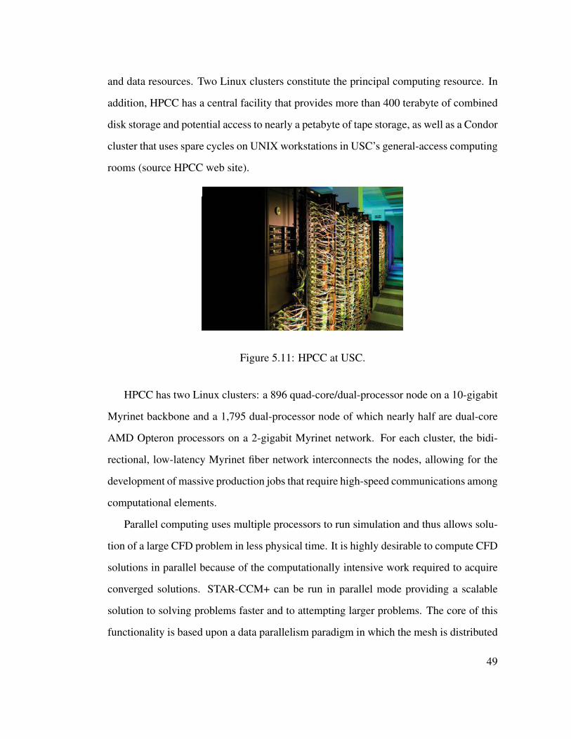
and data resources. Two Linux clusters constitute the principal computing resource. In
addition, HPCC has a central facility that provides more than 400 terabyte of combined
disk storage and potential access to nearly a petabyte of tape storage, as well as a Condor
cluster that uses spare cycles on UNIX workstations in USC’s general-access computing
rooms (source HPCC web site).
Figure 5.11: HPCC at USC.
HPCC has two Linux clusters: a 896 quad-core/dual-processor node on a 10-gigabit
Myrinet backbone and a 1,795 dual-processor node of which nearly half are dual-core
AMD Opteron processors on a 2-gigabit Myrinet network. For each cluster, the bidi-
rectional, low-latency Myrinet fiber network interconnects the nodes, allowing for the
development of massive production jobs that require high-speed communications among
computational elements.
Parallel computing uses multiple processors to run simulation and thus allows solu-
tion of a large CFD problem in less physical time. It is highly desirable to compute CFD
solutions in parallel because of the computationally intensive work required to acquire
converged solutions. STAR-CCM+ can be run in parallel mode providing a scalable
solution to solving problems faster and to attempting larger problems. The core of this
functionality is based upon a data parallelism paradigm in which the mesh is distributed
49
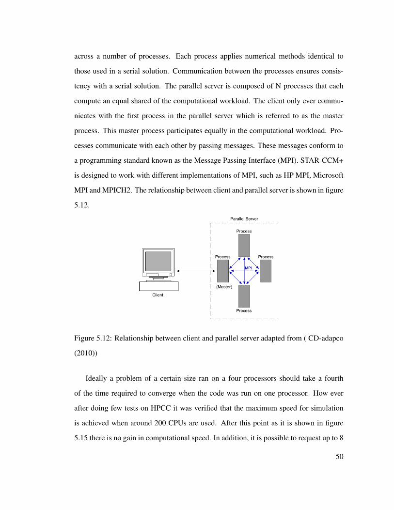
across a number of processes. Each process applies numerical methods identical to
those used in a serial solution. Communication between the processes ensures consis-
tency with a serial solution. The parallel server is composed of N processes that each
compute an equal shared of the computational workload. The client only ever commu-
nicates with the first process in the parallel server which is referred to as the master
process. This master process participates equally in the computational workload. Pro-
cesses communicate with each other by passing messages. These messages conform to
a programming standard known as the Message Passing Interface (MPI). STAR-CCM+
is designed to work with different implementations of MPI, such as HP MPI, Microsoft
MPI and MPICH2. The relationship between client and parallel server is shown in figure
5.12.
Figure 5.12: Relationship between client and parallel server adapted from ( CD-adapco
(2010))
Ideally a problem of a certain size ran on a four processors should take a fourth
of the time required to converge when the code was run on one processor. How ever
after doing few tests on HPCC it was verified that the maximum speed for simulation
is achieved when around 200 CPUs are used. After this point as it is shown in figure
5.15 there is no gain in computational speed. In addition, it is possible to request up to 8
50
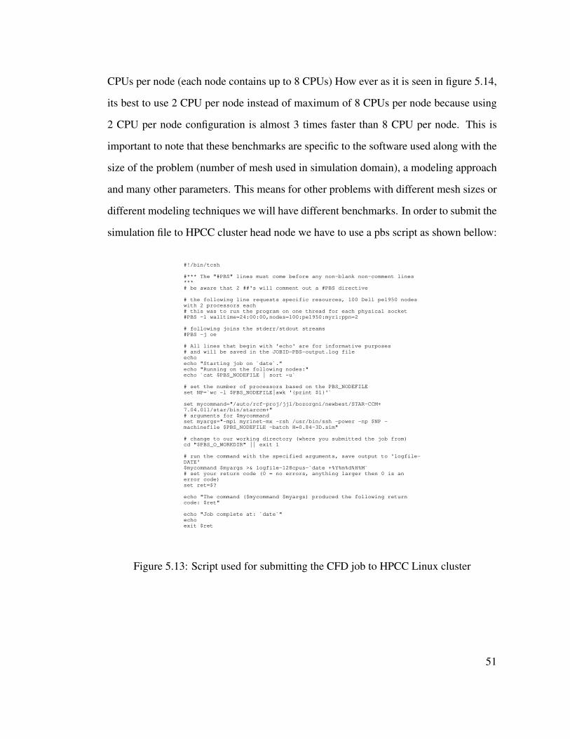
CPUs per node (each node contains up to 8 CPUs) How ever as it is seen in figure 5.14,
its best to use 2 CPU per node instead of maximum of 8 CPUs per node because using
2 CPU per node configuration is almost 3 times faster than 8 CPU per node. This is
important to note that these benchmarks are specific to the software used along with the
size of the problem (number of mesh used in simulation domain), a modeling approach
and many other parameters. This means for other problems with different mesh sizes or
different modeling techniques we will have different benchmarks. In order to submit the
simulation file to HPCC cluster head node we have to use a pbs script as shown bellow:
#!/bin/tcsh
#*** The "#PBS" lines must come before any non-blank non-comment lines ***# be aware that 2 ##'s will comment out a #PBS directive
# the following line requests specific resources, 100 Dell pe1950 nodes with 2 processors each# this was to run the program on one thread for each physical socket#PBS -l walltime=24:00:00,nodes=100:pe1950:myri:ppn=2
# following joins the stderr/stdout streams#PBS -j oe
# All lines that begin with 'echo' are for informative purposes# and will be saved in the JOBID-PBS-output.log fileechoecho "Starting job on `date`."echo "Running on the following nodes:"echo `cat $PBS_NODEFILE | sort -u`
# set the number of processors based on the PBS_NODEFILEset NP=`wc -l $PBS_NODEFILE|awk '{print $1}'`
set mycommand="/auto/rcf-proj/jjl/bozorgni/newbest/STAR-CCM+7.04.011/star/bin/starccm+"# arguments for $mycommandset myargs="-mpi myrinet-mx -rsh /usr/bin/ssh -power -np $NP -machinefile $PBS_NODEFILE -batch H=0.84-3D.sim"
# change to our working directory (where you submitted the job from)cd "$PBS_O_WORKDIR" || exit 1
# run the command with the specified arguments, save output to 'logfile-DATE'$mycommand $myargs >& logfile-128cpus-`date +%Y%m%d%H%M`# set your return code (0 = no errors, anything larger then 0 is an error code)set ret=$?
echo "The command ($mycommand $myargs) produced the following return code: $ret"
echo "Job complete at: `date`"echoexit $ret
Figure 5.13: Script used for submitting the CFD job to HPCC Linux cluster
51
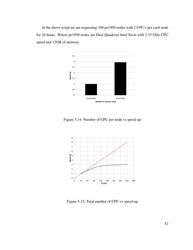
In the above script we are requesting 100 pe1950 nodes with 2 CPU’s per each node
for 24 hours. Where pe1950 nodes are Dual Quadcore Intel Xeon with 2.33 GHz CPU
speed and 12GB of memory.
0
0.5
1
1.5
2
2.5
3
3.5
8 cpu/node 2cpu/node
Sp
ee
d-u
p
Number of cpu per node
Figure 5.14: Number of CPU per node vs speed-up
0
1
2
3
4
5
6
7
8
9
0 32 64 96 128 160 192 224 256 288
Sp
ee
d-u
p
# CPUs
Figure 5.15: Total number of CPU vs speed-up
52
5.3 Numerical Methodology and Solver Parameters
STAR-CCM+ was configured to model the forces on the bridge deck in simulations.
Building the CFD model involves selecting mesh resolution, simulation algorithm,
boundary condition including air-water interface properties and turbulent model if
required. In addition to testing the ability of numerical model to replicate the experimen-
tal data, the CFD simulation had secondary objective of determining best model setup
to achieve most accurate simulation results. Several 2D and 3D models with different
mesh sizes and time steps are tested. The CFD simulation were conducted with an eye on
the efficiency of computational time. Even with HPCC facility, the high computational
intensity of CFD modeling demands an efficient model setup to ensure manageable run
time. The 2D and 3D simulations were solved as isothermal (the temperature in the
simulation domain was kept constant). The governing equation for 2D and 3D models
first solved as inviscid. Inviscid simulation are the Euler equations described in chapter
3. Solving Euler equation will generate the local pressure and velocity components of
fluid. STAR-CCM+’s multiphase segregated flow model is used to separate governing
equation for both the water and air. The Segregated Flow solver controls the solution
update for the Segregated Flow model according to the SIMPLE algorithm Ferziger
et al. (2002). It controls two additional solvers: velocity solver and pressure solver.
The velocity solver controls the under-relaxation factor and algebraic multigrid param-
eters for the momentum equations. More specifically, it solves the discretized momen-
tum equation to obtain the intermediate velocity field. The pressure solver controls the
under-relaxation factor and algebraic multigrid parameters for the pressure correction
equation. More specifically, it solves the discrete equation for pressure correction, and
updates the pressure field ( CD-adapco (2010)). Water is modeled as incompressible
fluid with density of ρ = 997.561 kg/m3 while air is modeled as a compressible ideal
53
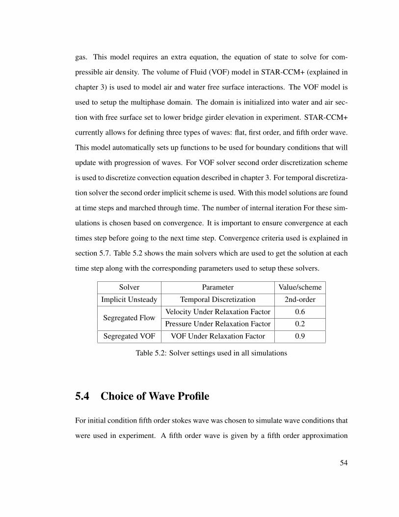
gas. This model requires an extra equation, the equation of state to solve for com-
pressible air density. The volume of Fluid (VOF) model in STAR-CCM+ (explained in
chapter 3) is used to model air and water free surface interactions. The VOF model is
used to setup the multiphase domain. The domain is initialized into water and air sec-
tion with free surface set to lower bridge girder elevation in experiment. STAR-CCM+
currently allows for defining three types of waves: flat, first order, and fifth order wave.
This model automatically sets up functions to be used for boundary conditions that will
update with progression of waves. For VOF solver second order discretization scheme
is used to discretize convection equation described in chapter 3. For temporal discretiza-
tion solver the second order implicit scheme is used. With this model solutions are found
at time steps and marched through time. The number of internal iteration For these sim-
ulations is chosen based on convergence. It is important to ensure convergence at each
times step before going to the next time step. Convergence criteria used is explained in
section 5.7. Table 5.2 shows the main solvers which are used to get the solution at each
time step along with the corresponding parameters used to setup these solvers.
Solver Parameter Value/scheme
Implicit Unsteady Temporal Discretization 2nd-order
Segregated FlowVelocity Under Relaxation Factor 0.6
Pressure Under Relaxation Factor 0.2
Segregated VOF VOF Under Relaxation Factor 0.9
Table 5.2: Solver settings used in all simulations
5.4 Choice of Wave Profile
For initial condition fifth order stokes wave was chosen to simulate wave conditions that
were used in experiment. A fifth order wave is given by a fifth order approximation
54
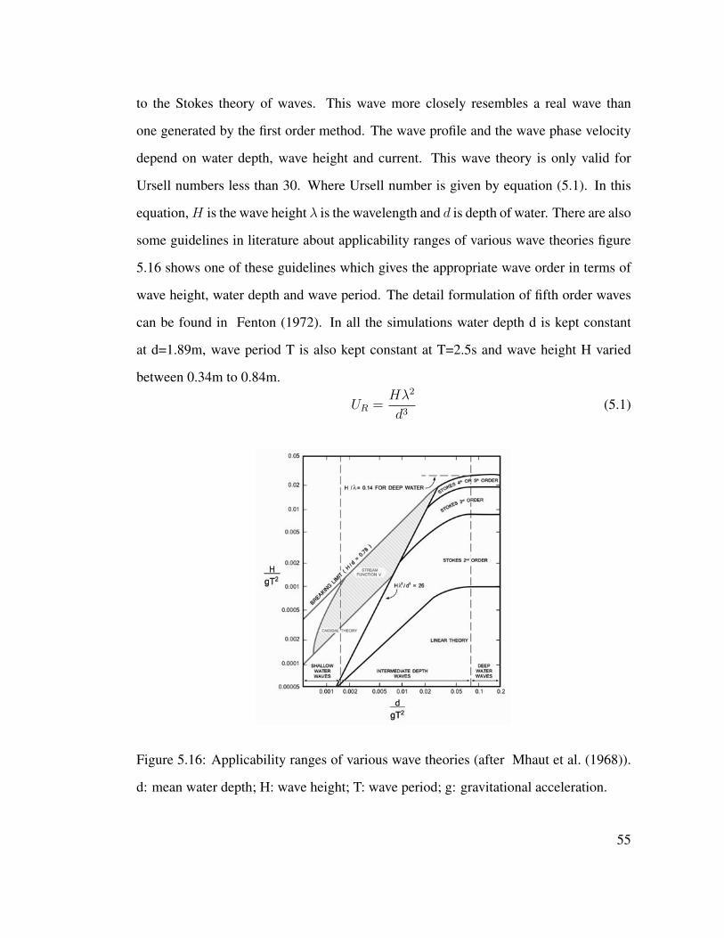
to the Stokes theory of waves. This wave more closely resembles a real wave than
one generated by the first order method. The wave profile and the wave phase velocity
depend on water depth, wave height and current. This wave theory is only valid for
Ursell numbers less than 30. Where Ursell number is given by equation (5.1). In this
equation, H is the wave height λ is the wavelength and d is depth of water. There are also
some guidelines in literature about applicability ranges of various wave theories figure
5.16 shows one of these guidelines which gives the appropriate wave order in terms of
wave height, water depth and wave period. The detail formulation of fifth order waves
can be found in Fenton (1972). In all the simulations water depth d is kept constant
at d=1.89m, wave period T is also kept constant at T=2.5s and wave height H varied
between 0.34m to 0.84m.
UR =Hλ2
d3(5.1)
Figure 5.16: Applicability ranges of various wave theories (after Mhaut et al. (1968)).
d: mean water depth; H: wave height; T: wave period; g: gravitational acceleration.
55

Figure 5.17 shows the wave generated using Stokes fifth order theory propagating
from left to right in simulation domain for wave amplitude H=0.5m and wave period
T=2.5s.
Figure 5.17: Incident wave generated using stokes fifth order theory for H=0.5m and
T=2.5 s
5.5 Choice of Boundary Conditions
Choice of boundary conditions is very important because it directly influences the sim-
ulation results. Following boundary conditions are used in the wave-bridge interaction
simulations and are explained in detail:
• Wall
• Velocity Inlet
• Pressure Outlet
• Symmetry Plane
A wall boundary represents an impermeable surface. An impenetrable boundary for
inviscid flows an impenetrable, no-slip boundary for viscous flow simulations. A pres-
sure outlet boundary is a flow outlet boundary at which the pressure is specified. A
velocity inlet boundary represents the inlet of a duct at which the flow velocity is known.
For the wall boundary condition, the normal velocity is explicitly set to zero. The bound-
ary face pressure is extrapolated from the adjacent cell using reconstruction gradients.
56
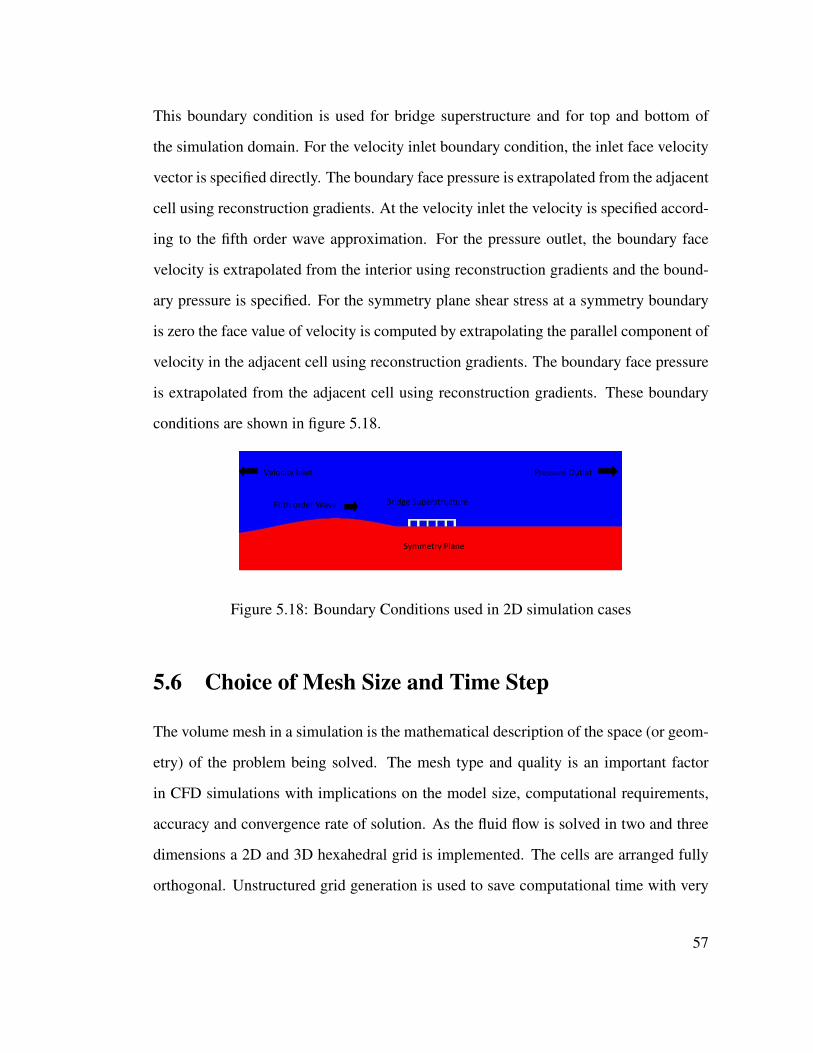
This boundary condition is used for bridge superstructure and for top and bottom of
the simulation domain. For the velocity inlet boundary condition, the inlet face velocity
vector is specified directly. The boundary face pressure is extrapolated from the adjacent
cell using reconstruction gradients. At the velocity inlet the velocity is specified accord-
ing to the fifth order wave approximation. For the pressure outlet, the boundary face
velocity is extrapolated from the interior using reconstruction gradients and the bound-
ary pressure is specified. For the symmetry plane shear stress at a symmetry boundary
is zero the face value of velocity is computed by extrapolating the parallel component of
velocity in the adjacent cell using reconstruction gradients. The boundary face pressure
is extrapolated from the adjacent cell using reconstruction gradients. These boundary
conditions are shown in figure 5.18.
Velocity Inlet Pressure Outlet
Fifth order Wave Bridge Superstructure
Symmetry Plane
Figure 5.18: Boundary Conditions used in 2D simulation cases
5.6 Choice of Mesh Size and Time Step
The volume mesh in a simulation is the mathematical description of the space (or geom-
etry) of the problem being solved. The mesh type and quality is an important factor
in CFD simulations with implications on the model size, computational requirements,
accuracy and convergence rate of solution. As the fluid flow is solved in two and three
dimensions a 2D and 3D hexahedral grid is implemented. The cells are arranged fully
orthogonal. Unstructured grid generation is used to save computational time with very
57
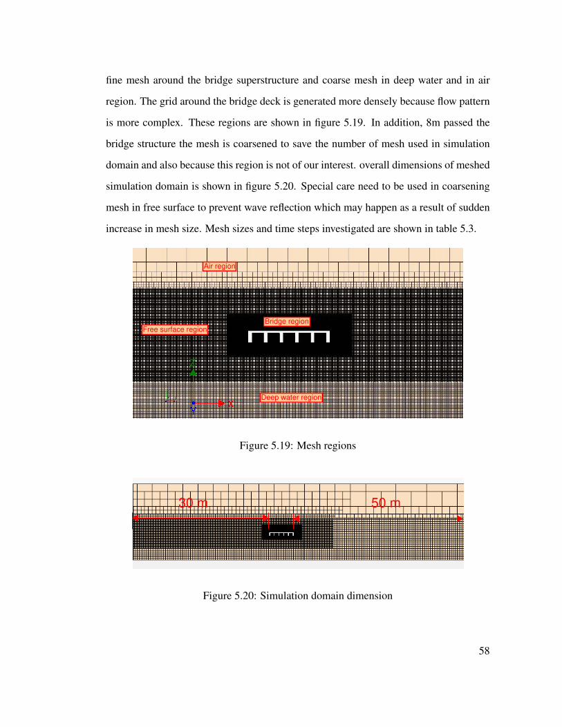
fine mesh around the bridge superstructure and coarse mesh in deep water and in air
region. The grid around the bridge deck is generated more densely because flow pattern
is more complex. These regions are shown in figure 5.19. In addition, 8m passed the
bridge structure the mesh is coarsened to save the number of mesh used in simulation
domain and also because this region is not of our interest. overall dimensions of meshed
simulation domain is shown in figure 5.20. Special care need to be used in coarsening
mesh in free surface to prevent wave reflection which may happen as a result of sudden
increase in mesh size. Mesh sizes and time steps investigated are shown in table 5.3.
Air region
Free surface regionBridge region
Deep water regionX
Z
Y
Figure 5.19: Mesh regions
30 m 50 m
Figure 5.20: Simulation domain dimension
58
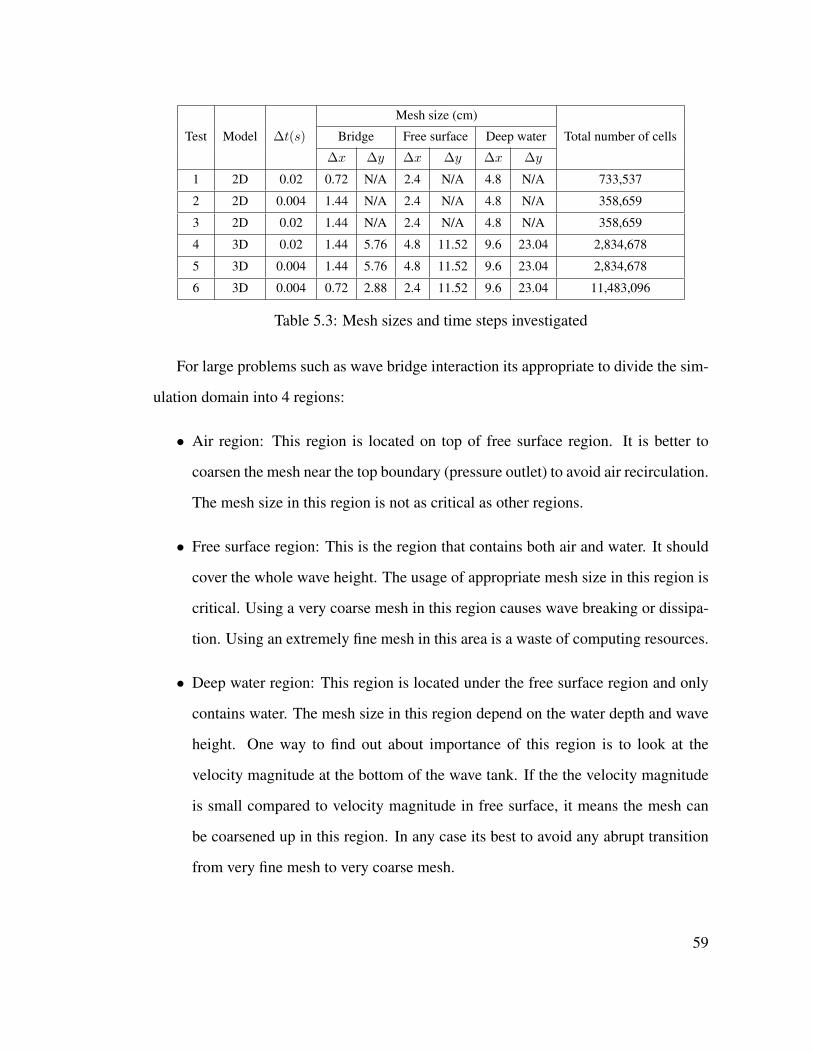
Test Model ∆t(s)
Mesh size (cm)
Total number of cellsBridge Free surface Deep water
∆x ∆y ∆x ∆y ∆x ∆y
1 2D 0.02 0.72 N/A 2.4 N/A 4.8 N/A 733,537
2 2D 0.004 1.44 N/A 2.4 N/A 4.8 N/A 358,659
3 2D 0.02 1.44 N/A 2.4 N/A 4.8 N/A 358,659
4 3D 0.02 1.44 5.76 4.8 11.52 9.6 23.04 2,834,678
5 3D 0.004 1.44 5.76 4.8 11.52 9.6 23.04 2,834,678
6 3D 0.004 0.72 2.88 2.4 11.52 9.6 23.04 11,483,096
Table 5.3: Mesh sizes and time steps investigated
For large problems such as wave bridge interaction its appropriate to divide the sim-
ulation domain into 4 regions:
• Air region: This region is located on top of free surface region. It is better to
coarsen the mesh near the top boundary (pressure outlet) to avoid air recirculation.
The mesh size in this region is not as critical as other regions.
• Free surface region: This is the region that contains both air and water. It should
cover the whole wave height. The usage of appropriate mesh size in this region is
critical. Using a very coarse mesh in this region causes wave breaking or dissipa-
tion. Using an extremely fine mesh in this area is a waste of computing resources.
• Deep water region: This region is located under the free surface region and only
contains water. The mesh size in this region depend on the water depth and wave
height. One way to find out about importance of this region is to look at the
velocity magnitude at the bottom of the wave tank. If the the velocity magnitude
is small compared to velocity magnitude in free surface, it means the mesh can
be coarsened up in this region. In any case its best to avoid any abrupt transition
from very fine mesh to very coarse mesh.
59
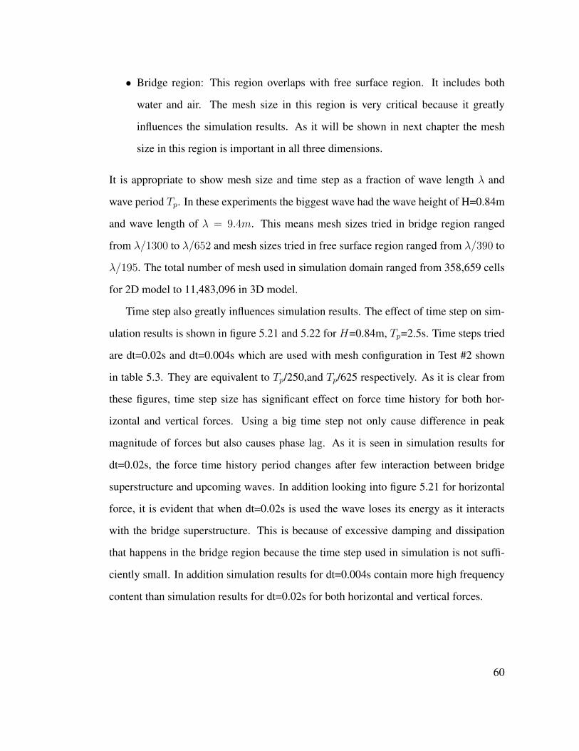
• Bridge region: This region overlaps with free surface region. It includes both
water and air. The mesh size in this region is very critical because it greatly
influences the simulation results. As it will be shown in next chapter the mesh
size in this region is important in all three dimensions.
It is appropriate to show mesh size and time step as a fraction of wave length λ and
wave period Tp. In these experiments the biggest wave had the wave height of H=0.84m
and wave length of λ = 9.4m. This means mesh sizes tried in bridge region ranged
from λ/1300 to λ/652 and mesh sizes tried in free surface region ranged from λ/390 to
λ/195. The total number of mesh used in simulation domain ranged from 358,659 cells
for 2D model to 11,483,096 in 3D model.
Time step also greatly influences simulation results. The effect of time step on sim-
ulation results is shown in figure 5.21 and 5.22 for H=0.84m, Tp=2.5s. Time steps tried
are dt=0.02s and dt=0.004s which are used with mesh configuration in Test #2 shown
in table 5.3. They are equivalent to Tp/250,and Tp/625 respectively. As it is clear from
these figures, time step size has significant effect on force time history for both hor-
izontal and vertical forces. Using a big time step not only cause difference in peak
magnitude of forces but also causes phase lag. As it is seen in simulation results for
dt=0.02s, the force time history period changes after few interaction between bridge
superstructure and upcoming waves. In addition looking into figure 5.21 for horizontal
force, it is evident that when dt=0.02s is used the wave loses its energy as it interacts
with the bridge superstructure. This is because of excessive damping and dissipation
that happens in the bridge region because the time step used in simulation is not suffi-
ciently small. In addition simulation results for dt=0.004s contain more high frequency
content than simulation results for dt=0.02s for both horizontal and vertical forces.
60
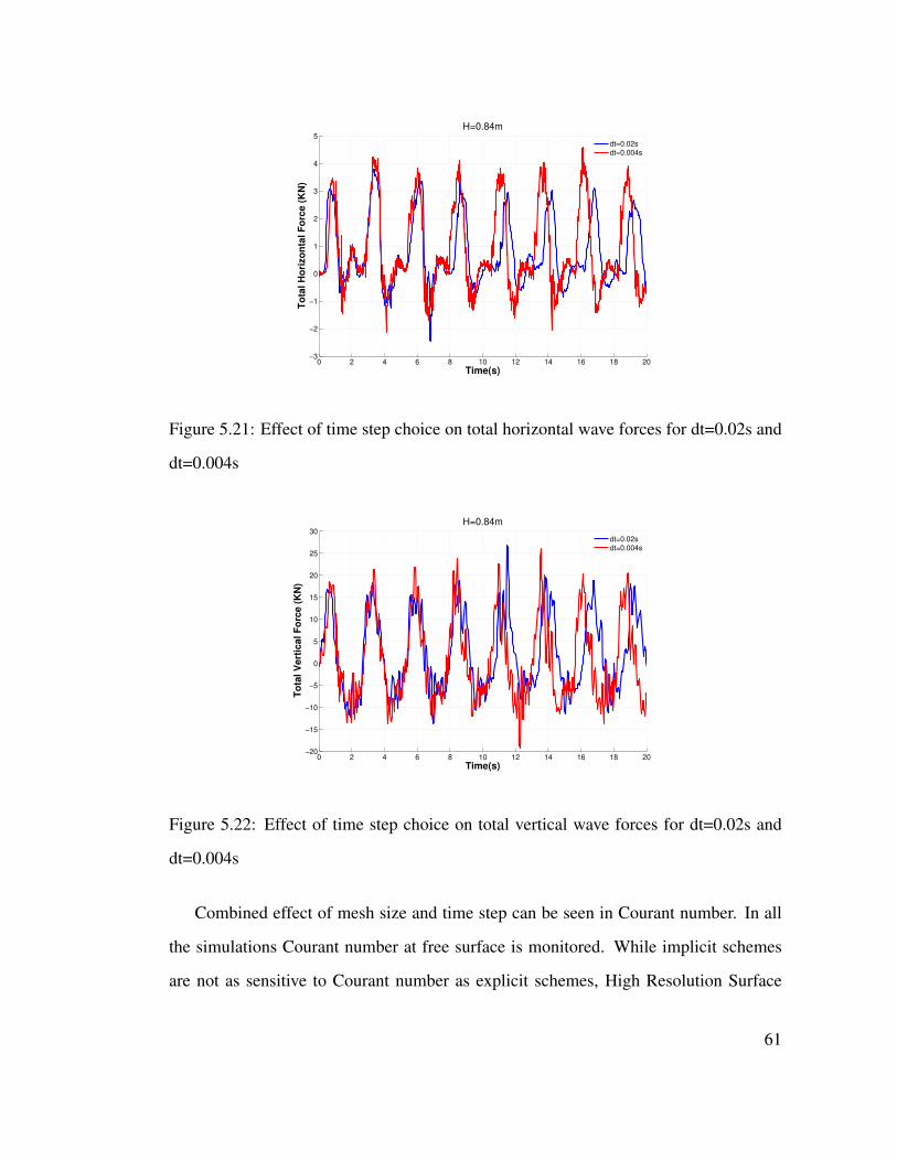
0 2 4 6 8 10 12 14 16 18 20−3
−2
−1
0
1
2
3
4
5
Time(s)
To
tal H
ori
zo
nta
l F
orc
e (
KN
)
H=0.84m
dt=0.02s
dt=0.004s
Figure 5.21: Effect of time step choice on total horizontal wave forces for dt=0.02s and
dt=0.004s
0 2 4 6 8 10 12 14 16 18 20−20
−15
−10
−5
0
5
10
15
20
25
30
Time(s)
To
tal V
ert
ical F
orc
e (
KN
)
H=0.84m
dt=0.02s
dt=0.004s
Figure 5.22: Effect of time step choice on total vertical wave forces for dt=0.02s and
dt=0.004s
Combined effect of mesh size and time step can be seen in Courant number. In all
the simulations Courant number at free surface is monitored. While implicit schemes
are not as sensitive to Courant number as explicit schemes, High Resolution Surface
61
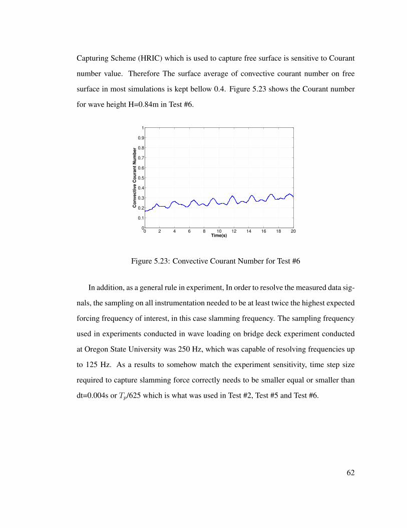
Capturing Scheme (HRIC) which is used to capture free surface is sensitive to Courant
number value. Therefore The surface average of convective courant number on free
surface in most simulations is kept bellow 0.4. Figure 5.23 shows the Courant number
for wave height H=0.84m in Test #6.
0 2 4 6 8 10 12 14 16 18 200
0.1
0.2
0.3
0.4
0.5
0.6
0.7
0.8
0.9
1
Time(s)
Co
nvecti
ve C
ou
ran
t N
um
ber
Figure 5.23: Convective Courant Number for Test #6
In addition, as a general rule in experiment, In order to resolve the measured data sig-
nals, the sampling on all instrumentation needed to be at least twice the highest expected
forcing frequency of interest, in this case slamming frequency. The sampling frequency
used in experiments conducted in wave loading on bridge deck experiment conducted
at Oregon State University was 250 Hz, which was capable of resolving frequencies up
to 125 Hz. As a results to somehow match the experiment sensitivity, time step size
required to capture slamming force correctly needs to be smaller equal or smaller than
dt=0.004s or Tp/625 which is what was used in Test #2, Test #5 and Test #6.
62

5.7 Solution Convergence
The numerical method explained in chapter 3, requires an iterative process in order to
obtain a solution. After each iteration, residuals are produced that indicate how well the
governing equations for each solver quantity are being satisfied numerically. Residuals
are used as one of the means to judge solution convergence. In STAR-CCM+ they are
created automatically. While its true that residuals tend to decrease to a small num-
ber when solution is converged, the residual monitor alone, can not be relied on as the
only measure of convergence because the amount of decrease in residual depends on
the simulation. For example initial guess strongly influences the amount that residuals
decrease. If the initial guess satisfies the descretized equations perfectly, the residuals
will not drop at all. Also, residual plot in STAR-CCM+ is for the whole simulation
domain. In some cases because of poor mesh quality, dispersive errors may result in
oscillation in small number of cells which is out side the domain of our interest. In this
case the residual plot will show that the solution is not converged while the quantities of
interest inside our domain of interest is fully converged. Finally, residuals do not nec-
essarily relate to quantities of engineering interest in the simulation such as integrated
forces ( CD-adapco (2010)).
As a result in addition to the default residual plots in STAR-CCM+, we define two
additional engineering monitors for horizontal and vertical forces for each iteration.
Figure 5.24 shows an example of residual plot for the whole simulation domain for
continuity and momentum equation.
63
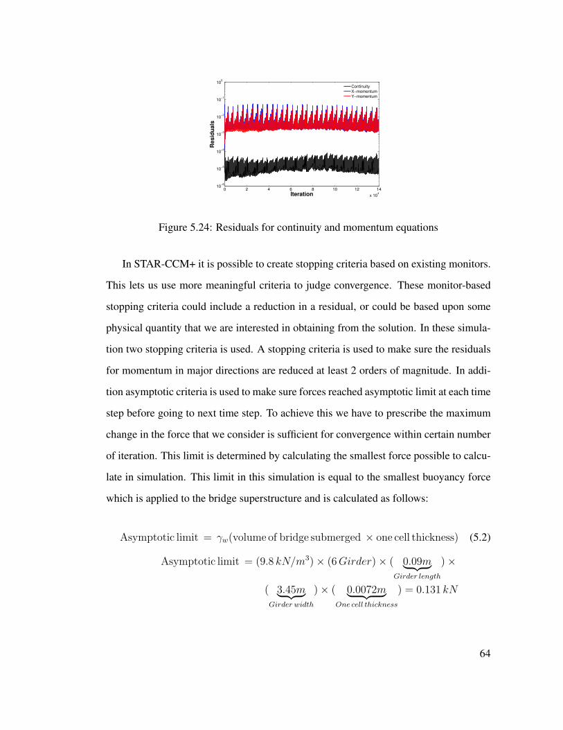
0 2 4 6 8 10 12 14
x 104
10−6
10−5
10−4
10−3
10−2
10−1
100
Iteration
Resid
uals
ContinuityX−momentumY−momentum
Figure 5.24: Residuals for continuity and momentum equations
In STAR-CCM+ it is possible to create stopping criteria based on existing monitors.
This lets us use more meaningful criteria to judge convergence. These monitor-based
stopping criteria could include a reduction in a residual, or could be based upon some
physical quantity that we are interested in obtaining from the solution. In these simula-
tion two stopping criteria is used. A stopping criteria is used to make sure the residuals
for momentum in major directions are reduced at least 2 orders of magnitude. In addi-
tion asymptotic criteria is used to make sure forces reached asymptotic limit at each time
step before going to next time step. To achieve this we have to prescribe the maximum
change in the force that we consider is sufficient for convergence within certain number
of iteration. This limit is determined by calculating the smallest force possible to calcu-
late in simulation. This limit in this simulation is equal to the smallest buoyancy force
which is applied to the bridge superstructure and is calculated as follows:
Asymptotic limit = γw(volume of bridge submerged × one cell thickness) (5.2)
Asymptotic limit = (9.8 kN/m3)× (6Girder)× ( 0.09m︸ ︷︷ ︸
Girder length
)×
( 3.45m︸ ︷︷ ︸
Girder width
)× ( 0.0072m︸ ︷︷ ︸
One cell thickness
) = 0.131 kN
64
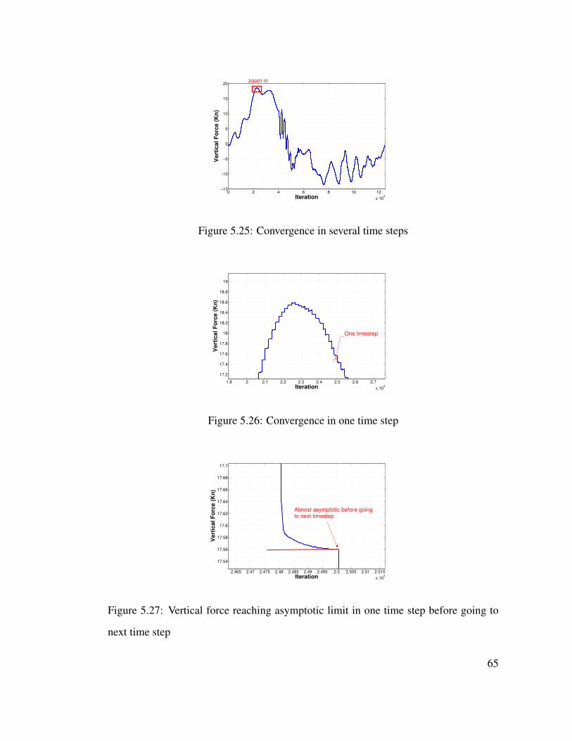
0 2 4 6 8 10 12
x 104
−15
−10
−5
0
5
10
15
20
Iteration
Vert
ical F
orc
e (
Kn
)
zoom in
Figure 5.25: Convergence in several time steps
1.9 2 2.1 2.2 2.3 2.4 2.5 2.6 2.7
x 104
17.2
17.4
17.6
17.8
18
18.2
18.4
18.6
18.8
19
Iteration
Ve
rtic
al F
orc
e (
Kn
)
One timestep
Figure 5.26: Convergence in one time step
2.465 2.47 2.475 2.48 2.485 2.49 2.495 2.5 2.505 2.51 2.515
x 104
17.54
17.56
17.58
17.6
17.62
17.64
17.66
17.68
17.7
Iteration
Ve
rtic
al
Fo
rce
(K
n)
Almost asymptotic before goingto next timestep
Figure 5.27: Vertical force reaching asymptotic limit in one time step before going to
next time step
65
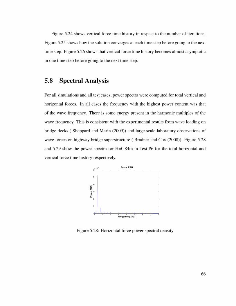
Figure 5.24 shows vertical force time history in respect to the number of iterations.
Figure 5.25 shows how the solution converges at each time step before going to the next
time step. Figure 5.26 shows that vertical force time history becomes almost asymptotic
in one time step before going to the next time step.
5.8 Spectral Analysis
For all simulations and all test cases, power spectra were computed for total vertical and
horizontal forces. In all cases the frequency with the highest power content was that
of the wave frequency. There is some energy present in the harmonic multiples of the
wave frequency. This is consistent with the experimental results from wave loading on
bridge decks ( Sheppard and Marin (2009)) and large scale laboratory observations of
wave forces on highway bridge superstructure ( Bradner and Cox (2008)). Figure 5.28
and 5.29 show the power spectra for H=0.84m in Test #6 for the total horizontal and
vertical force time history respectively.
0 1 2 3 4 5 6 7 80
1
2
3
4
5
6x 10
12
Frequency (Hz)
Fo
rce
PS
D
Force PSD
Figure 5.28: Horizontal force power spectral density
66
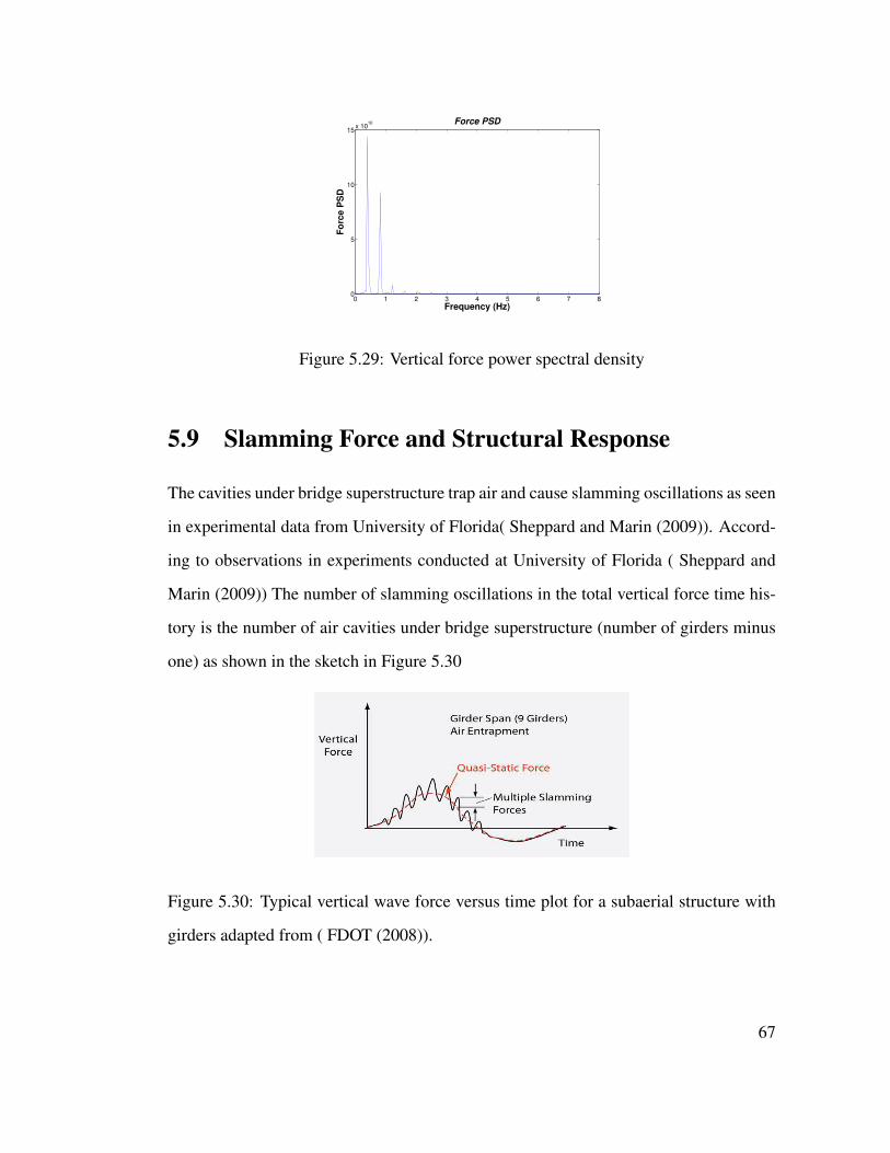
0 1 2 3 4 5 6 7 80
5
10
15x 10
10
Frequency (Hz)
Fo
rce P
SD
Force PSD
Figure 5.29: Vertical force power spectral density
5.9 Slamming Force and Structural Response
The cavities under bridge superstructure trap air and cause slamming oscillations as seen
in experimental data from University of Florida( Sheppard and Marin (2009)). Accord-
ing to observations in experiments conducted at University of Florida ( Sheppard and
Marin (2009)) The number of slamming oscillations in the total vertical force time his-
tory is the number of air cavities under bridge superstructure (number of girders minus
one) as shown in the sketch in Figure 5.30
Figure 5.30: Typical vertical wave force versus time plot for a subaerial structure with
girders adapted from ( FDOT (2008)).
67
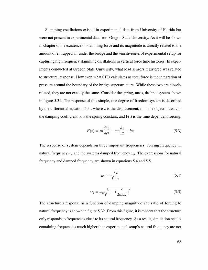
Slamming oscillations existed in experimental data from University of Florida but
were not present in experimental data from Oregon State University. As it will be shown
in chapter 6, the existence of slamming force and its magnitude is directly related to the
amount of entrapped air under the bridge and the sensitiveness of experimental setup for
capturing high frequency slamming oscillations in vertical force time histories. In exper-
iments conducted at Oregon State University, what load sensors registered was related
to structural response. How ever, what CFD calculates as total force is the integration of
pressure around the boundary of the bridge superstructure. While these two are closely
related, they are not exactly the same. Consider the spring, mass, dashpot system shown
in figure 5.31. The response of this simple, one degree of freedom system is described
by the differential equation 5.3 , where z is the displacement, m is the object mass, c is
the damping coefficient, k is the spring constant, and F(t) is the time dependent forcing.
F (t) = md2z
dt2+ cm
dz
dt+ kz (5.3)
The response of system depends on three important frequencies: forcing frequency ω,
natural frequency ωn and the systems damped frequency ωd. The expressions for natural
frequency and damped frequency are shown in equations 5.4 and 5.5.
ωn =
√
k
m(5.4)
ωd = ωn
√
1− (c
2mωn
)2
(5.5)
The structure’s response as a function of damping magnitude and ratio of forcing to
natural frequency is shown in figure 5.32. From this figure, it is evident that the structure
only responds to frequencies close to its natural frequency. As a result, simulation results
containing frequencies much higher than experimental setup’s natural frequency are not
68
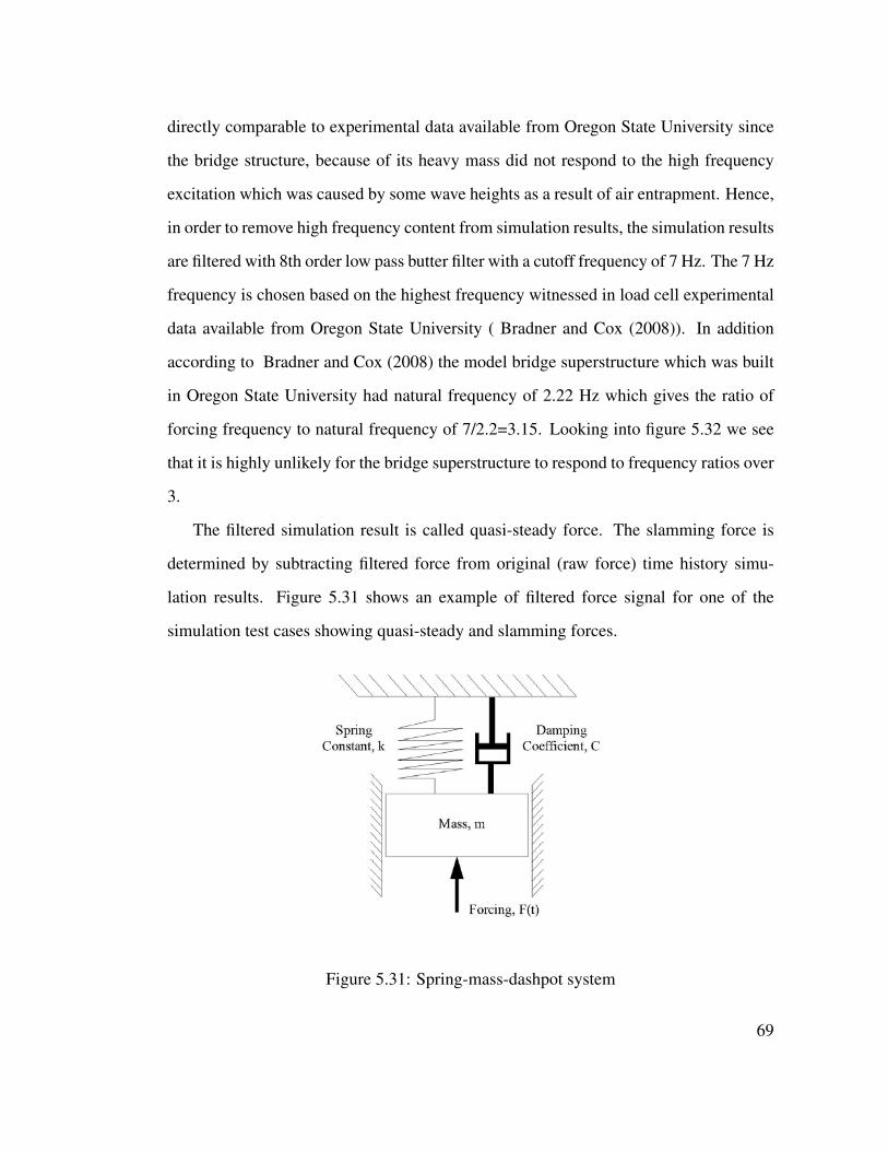
directly comparable to experimental data available from Oregon State University since
the bridge structure, because of its heavy mass did not respond to the high frequency
excitation which was caused by some wave heights as a result of air entrapment. Hence,
in order to remove high frequency content from simulation results, the simulation results
are filtered with 8th order low pass butter filter with a cutoff frequency of 7 Hz. The 7 Hz
frequency is chosen based on the highest frequency witnessed in load cell experimental
data available from Oregon State University ( Bradner and Cox (2008)). In addition
according to Bradner and Cox (2008) the model bridge superstructure which was built
in Oregon State University had natural frequency of 2.22 Hz which gives the ratio of
forcing frequency to natural frequency of 7/2.2=3.15. Looking into figure 5.32 we see
that it is highly unlikely for the bridge superstructure to respond to frequency ratios over
3.
The filtered simulation result is called quasi-steady force. The slamming force is
determined by subtracting filtered force from original (raw force) time history simu-
lation results. Figure 5.31 shows an example of filtered force signal for one of the
simulation test cases showing quasi-steady and slamming forces.
ass-dashpot system
Figure 5.31: Spring-mass-dashpot system
69
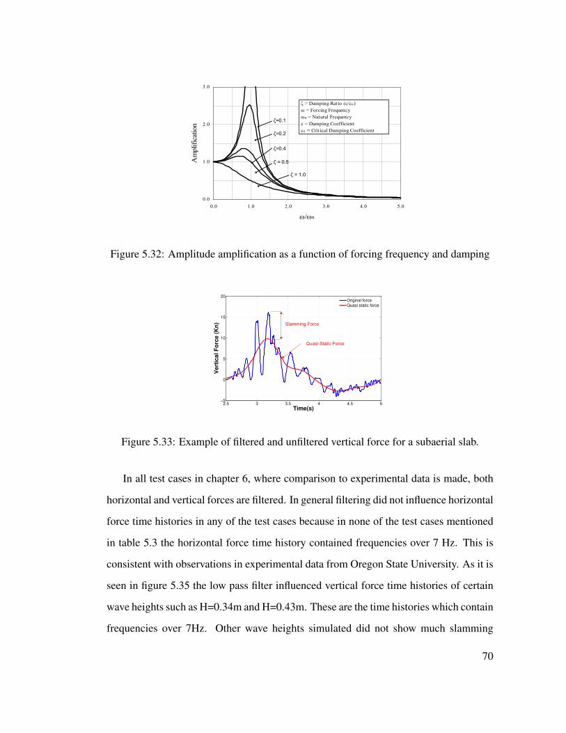
0.0
1.0
2.0
3.0
0.0 1.0 2.0 3.0 4.0 5.0
ω/ωn
Am
plifi
cation ζ=0.1
ζ=0.2
ζ=0.4
ζ = 0.5
ζ = 1.0
ζ = Damping Ratio (c/co)
ω = Forcing Frequency
ωn = Natural Frequency
c = Damping Coefficient
co = Critical Damping Coefficient
Figure 5.32: Amplitude amplification as a function of forcing frequency and damping
2.5 3 3.5 4 4.5 5−5
0
5
10
15
20
Time(s)
Ve
rtic
al F
orc
e (
Kn
)
Original force
Quasi static force
Slamming Force
Quasi-Static Force
Figure 5.33: Example of filtered and unfiltered vertical force for a subaerial slab.
In all test cases in chapter 6, where comparison to experimental data is made, both
horizontal and vertical forces are filtered. In general filtering did not influence horizontal
force time histories in any of the test cases because in none of the test cases mentioned
in table 5.3 the horizontal force time history contained frequencies over 7 Hz. This is
consistent with observations in experimental data from Oregon State University. As it is
seen in figure 5.35 the low pass filter influenced vertical force time histories of certain
wave heights such as H=0.34m and H=0.43m. These are the time histories which contain
frequencies over 7Hz. Other wave heights simulated did not show much slamming
70
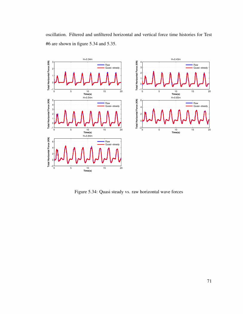
oscillation. Filtered and unfiltered horizontal and vertical force time histories for Test
#6 are shown in figure 5.34 and 5.35.
0 5 10 15 20−1
0
1
2
3
Time(s)
To
tal
Ho
rizo
nta
l F
orc
e (
KN
)
H=0.34m
Raw
Quasi−steady
0 5 10 15 20−1
0
1
2
3
4
Time(s)
To
tal
Ho
rizo
nta
l F
orc
e (
KN
)
H=0.43m
Raw
Quasi−steady
0 5 10 15 20−1
0
1
2
3
4
5
Time(s)
To
tal
Ho
rizo
nta
l F
orc
e (
KN
)
H=0.54m
Raw
Quasi−steady
0 5 10 15 20−2
0
2
4
6
Time(s)
To
tal
Ho
rizo
nta
l F
orc
e (
KN
)
H=0.65m
Raw
Quasi−steady
0 5 10 15 20−2
0
2
4
6
Time(s)
To
tal
Ho
rizo
nta
l F
orc
e (
KN
)
H=0.84m
Raw
Quasi−steady
Figure 5.34: Quasi steady vs. raw horizontal wave forces
71
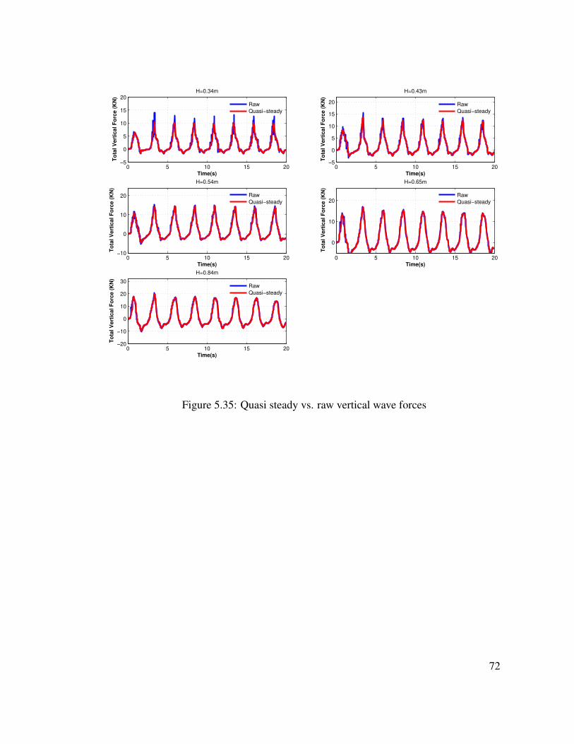
0 5 10 15 20−5
0
5
10
15
20
Time(s)
To
tal
Ve
rtic
al
Fo
rce
(K
N)
H=0.34m
Raw
Quasi−steady
0 5 10 15 20−5
0
5
10
15
20
Time(s)
To
tal
Ve
rtic
al
Fo
rce
(K
N)
H=0.43m
Raw
Quasi−steady
0 5 10 15 20−10
0
10
20
Time(s)
To
tal
Ve
rtic
al
Fo
rce
(K
N)
H=0.54m
Raw
Quasi−steady
0 5 10 15 20
0
10
20
Time(s)
To
tal
Ve
rtic
al
Fo
rce
(K
N)
H=0.65m
Raw
Quasi−steady
0 5 10 15 20−20
−10
0
10
20
30
Time(s)
To
tal
Ve
rtic
al
Fo
rce
(K
N)
H=0.84m
Raw
Quasi−steady
Figure 5.35: Quasi steady vs. raw vertical wave forces
72
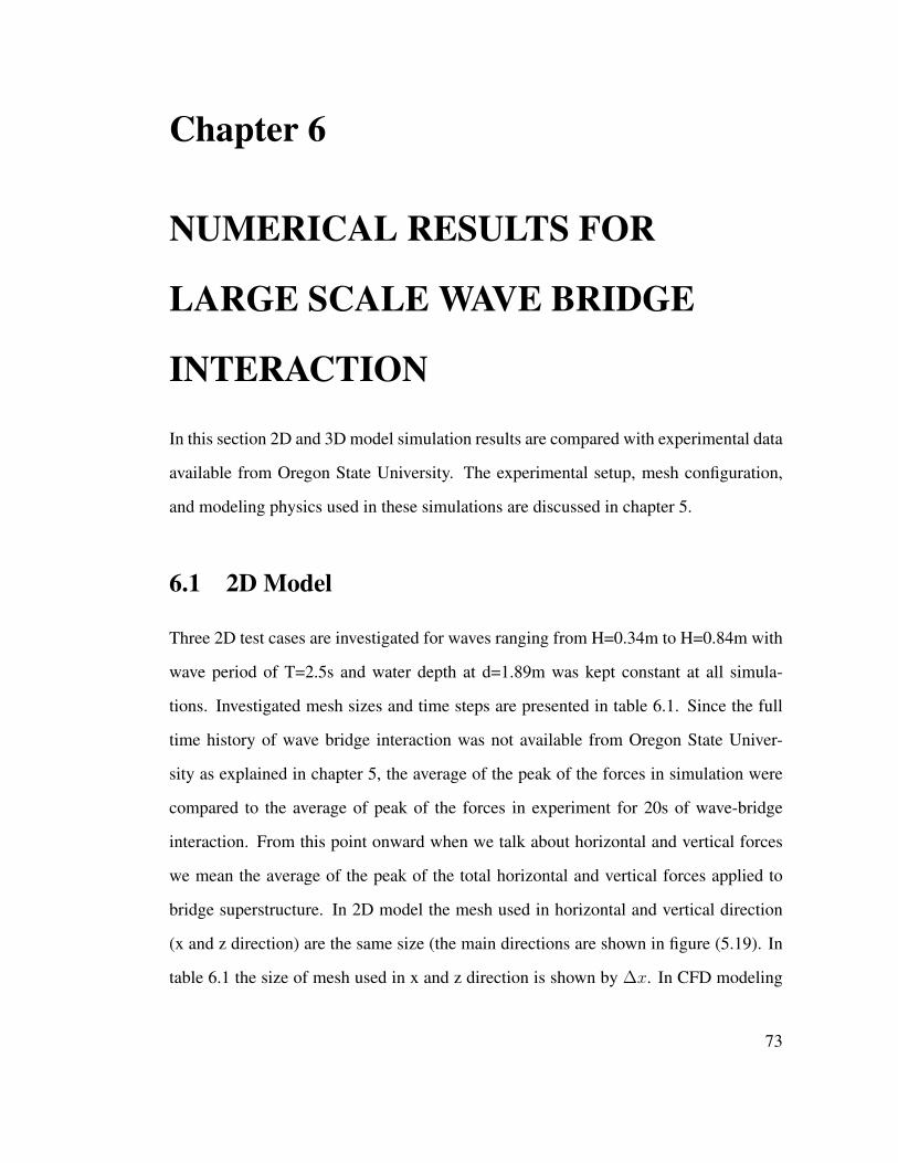
Chapter 6
NUMERICAL RESULTS FOR
LARGE SCALE WAVE BRIDGE
INTERACTION
In this section 2D and 3D model simulation results are compared with experimental data
available from Oregon State University. The experimental setup, mesh configuration,
and modeling physics used in these simulations are discussed in chapter 5.
6.1 2D Model
Three 2D test cases are investigated for waves ranging from H=0.34m to H=0.84m with
wave period of T=2.5s and water depth at d=1.89m was kept constant at all simula-
tions. Investigated mesh sizes and time steps are presented in table 6.1. Since the full
time history of wave bridge interaction was not available from Oregon State Univer-
sity as explained in chapter 5, the average of the peak of the forces in simulation were
compared to the average of peak of the forces in experiment for 20s of wave-bridge
interaction. From this point onward when we talk about horizontal and vertical forces
we mean the average of the peak of the total horizontal and vertical forces applied to
bridge superstructure. In 2D model the mesh used in horizontal and vertical direction
(x and z direction) are the same size (the main directions are shown in figure (5.19). In
table 6.1 the size of mesh used in x and z direction is shown by ∆x. In CFD modeling
73

Test Model ∆t(s)
Mesh size (cm)
Total # of cellsBridge Free surface Deep water
∆x ∆y ∆x ∆y ∆x ∆y
1 2D 0.02 0.72 N/A 2.4 N/A 4.8 N/A 733,537
2 2D 0.004 1.44 N/A 2.4 N/A 4.8 N/A 358,659
3 2D (pressure outlet) 0.02 1.44 N/A 2.4 N/A 4.8 N/A 358,659
Table 6.1: Different mesh sizes and time steps investigated in 2D model
of wave propagation, it is possible to use a different size mesh in x and z direction. In
general since z direction is more critical in free surface wave modeling, the mesh in z
direction can be refined to lessen excessive wave energy dissipation and save on compu-
tational time. How ever in problem of wave interacting with bridge superstructure, we
noticed abnormal elongation of wave as it hit the bridge when the bigger mesh size was
used in x direction. To avoid this problem, In all simulation cases the mesh used in x
and z direction are the same size and they are simply shown by ∆x.
6.1.1 Simulation Results for Test #1
In Test #1 the time step used is dt=0.02s which is equivalent to Tp/125. Horizontal force
time history for H=0.34m to H=0.84m is shown in Figure 6.1. In Figure 6.1 the blue
graph is simulated horizontal force time history, the discrete blue horizontal line is the
average of peak of the forces in simulation, and the discrete black horizontal line is the
average of peak of the forces in experiment. As it is seen in figure 6.1, for all wave
heights, simulation under predicts the horizontal force. As the wave height increase,
the magnitude of error also increase. The maximum error in horizontal force predic-
tions happens for wave height of H=0.84m and is 48 percent. The vertical force time
history is shown in figure 6.2. As it is seen in figure 6.2 simulation over predicts the
magnitude of vertical forces for H=0.34m, H=0.43m and H=0.54m and under predicts
the magnitude of vertical forces for H=0.65 and H=0.84m. For H=0.34m, simulation
74

over predicts the magnitude of vertical forces by 20 percent. For H=0.84m, the simula-
tion under predicts the magnitude of vertical forces by 18 percent. Figure 6.3 shows the
comparison between the average of peak of the forces in experiment and average of the
peak of the forces in simulation for both horizontal and vertical forces applied to bridge
superstructure.
0 5 10 15 20
0
1
2
3
Time(s)
To
tal
Ho
rizo
nta
l F
orc
e (
KN
)
H=0.34m
Experiment
Simulation
0 5 10 15 20−1
0
1
2
3
4
Time(s)
To
tal
Ho
rizo
nta
l F
orc
e (
KN
)
H=0.43m
Experiment
Simulation
0 5 10 15 20−1
0
1
2
3
4
5
Time(s)
To
tal
Ho
rizo
nta
l F
orc
e (
KN
)
H=0.54m
Experiment
Simulation
0 5 10 15 20−2
0
2
4
6
Time(s)
To
tal
Ho
rizo
nta
l F
orc
e (
KN
)
H=0.65m
Experiment
Simulation
0 5 10 15 20
−2
0
2
4
6
8
10
Time(s)
To
tal
Ho
rizo
nta
l F
orc
e (
KN
)
H=0.81m
Experiment
Simulation
Figure 6.1: Horizontal force simulation results for Test #1
In this figure, hollow spheres are experimental data and the solid spheres are simula-
tion results. In figure 6.3 the horizontal error bar is the range of wave heights produced
by the wave maker. The vertical error bar represents the range of forces measured by
load sensor for the range of wave heights measured. The behavior of simulation force
time history is different in horizontal and vertical force time histories.
75
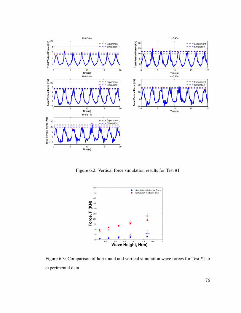
0 5 10 15 20
0
5
10
15
20
Time(s)
To
tal
Ve
rtic
al
Fo
rce
(K
N)
H=0.34m
Experiment
Simulation
0 5 10 15 20
0
5
10
15
20
Time(s)
To
tal
Ve
rtic
al
Fo
rce
(K
N)
H=0.43m
Experiment
Simulation
0 5 10 15 20
−5
0
5
10
15
20
Time(s)
To
tal
Ve
rtic
al
Fo
rce
(K
N)
H=0.54m
Experiment
Simulation
0 5 10 15 20−10
0
10
20
Time(s)
To
tal
Ve
rtic
al
Fo
rce
(K
N)
H=0.65m
Experiment
Simulation
0 5 10 15 20
−10
0
10
20
30
Time(s)
To
tal
Ve
rtic
al
Fo
rce
(K
N)
H=0.81m
Experiment
Simulation
Figure 6.2: Vertical force simulation results for Test #1
0.4 0.5 0.6 0.7 0.8 0.9 10
5
10
15
20
25
30
35
40
45
50
Wave Height, H(m)
Fo
rce, F
(K
N)
Simulation−Horizontal Force
Simulation−Vertical Force
Figure 6.3: Comparison of horizontal and vertical simulation wave forces for Test #1 to
experimental data
76
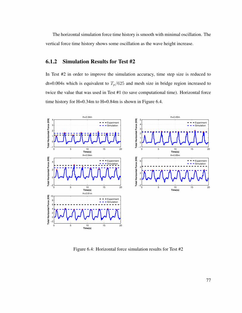
The horizontal simulation force time history is smooth with minimal oscillation. The
vertical force time history shows some oscillation as the wave height increase.
6.1.2 Simulation Results for Test #2
In Test #2 in order to improve the simulation accuracy, time step size is reduced to
dt=0.004s which is equivalent to Tp/625 and mesh size in bridge region increased to
twice the value that was used in Test #1 (to save computational time). Horizontal force
time history for H=0.34m to H=0.84m is shown in Figure 6.4.
0 5 10 15 20−1
0
1
2
3
4
Time(s)
To
tal
Ho
rizo
nta
l F
orc
e (
KN
)
H=0.34m
Experiment
Simulation
0 5 10 15 20−1
0
1
2
3
4
5
Time(s)
To
tal
Ho
rizo
nta
l F
orc
e (
KN
)
H=0.43m
Experiment
Simulation
0 5 10 15 20−2
0
2
4
Time(s)
To
tal
Ho
rizo
nta
l F
orc
e (
KN
)
H=0.54m
Experiment
Simulation
0 5 10 15 20−2
0
2
4
6
Time(s)
To
tal
Ho
rizo
nta
l F
orc
e (
KN
)
H=0.65m
Experiment
Simulation
0 5 10 15 20
−2
0
2
4
6
8
10
Time(s)
To
tal
Ho
rizo
nta
l F
orc
e (
KN
)
H=0.81m
Experiment
Simulation
Figure 6.4: Horizontal force simulation results for Test #2
77
The simulation over predicts the average of the peak of the horizontal forces for
H=0.34m while it under predicts the average of the peak of horizontal forces for the rest
of wave heights. The maximum error in horizontal force again happens for the biggest
wave height H=0.84m which is 37 percent. Comparing to Test #1, the maximum error in
horizontal wave forces reduced by 11 percent. The vertical wave force time history for
Test #2 is shown in figure 6.5. Comparing to Test #1 vertical forces, vertical force time
history in Test #2 shows a highly oscillatory behavior that is not seen in Test #1. As the
wave height increase, the oscillatory behavior in vertical force time history decrease.
Vertical force time history in Test #2 does not compare well with experimental data.
Highly oscillatory behavior that is seen in wave heights of H=0.34m, H=0.43m and
H=0.54m cause large errors in vertical force predictions. Simulation over predicts the
magnitude of vertical force for H=0.34m by as much as 93 percent. Test #2 simulation
under predicts the magnitude of vertical force for H=0.84m by 6 percent. This means
even though comparing to Test #1, the maximum error in horizontal forces reduced by
11 percent, the maximum error in vertical force predictions increased from 23 percent
to 93 percent.
78
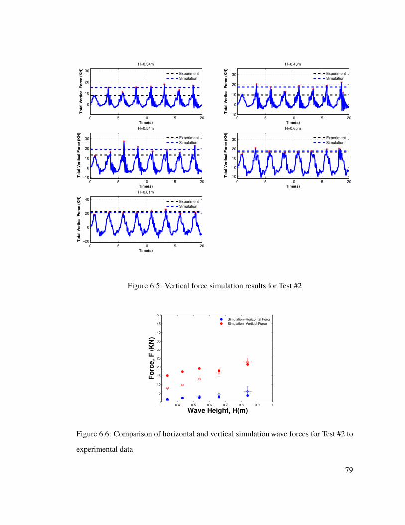
0 5 10 15 20
0
10
20
30
Time(s)
To
tal
Ve
rtic
al
Fo
rce
(K
N)
H=0.34m
Experiment
Simulation
0 5 10 15 20−10
0
10
20
30
Time(s)
To
tal
Ve
rtic
al
Fo
rce
(K
N)
H=0.43m
Experiment
Simulation
0 5 10 15 20−10
0
10
20
30
Time(s)
To
tal
Ve
rtic
al
Fo
rce
(K
N)
H=0.54m
Experiment
Simulation
0 5 10 15 20
−10
0
10
20
30
Time(s)
To
tal
Ve
rtic
al
Fo
rce
(K
N)
H=0.65m
Experiment
Simulation
0 5 10 15 20
−20
0
20
40
Time(s)
To
tal
Ve
rtic
al
Fo
rce
(K
N)
H=0.81m
Experiment
Simulation
Figure 6.5: Vertical force simulation results for Test #2
0.4 0.5 0.6 0.7 0.8 0.9 10
5
10
15
20
25
30
35
40
45
50
Wave Height, H(m)
Fo
rce, F
(K
N)
Simulation−Horizontal Force
Simulation−Vertical Force
Figure 6.6: Comparison of horizontal and vertical simulation wave forces for Test #2 to
experimental data
79
Some simulation scenes showing wave interacting with bridge deck for Test #2 is
shown for H=0.84m in figures 6.7 to 6.11. In the following figures: figure 6.7 shows
volume of fluid scene. In this figure red represents water and blue represents air and
all the colors in between represent mixture of air and water. Figure 6.7 shows that as
wave hits the bridge overtops it and part of it reflects back from the bridge and mixes
up with the upcoming wave. It is also evident in figure 6.7 that significant amount of
air gets trapped under the bridge deck inside the space between bridge girders because
as we see the water does not progress into the cavities under the bridge superstructure.
This is mainly due to the symmetry boundary used on the side of 2D simulation domain
which does not allow any air to exit from side of simulation domain. Figure 6.8 shows
the pressure distribution inside simulation domain. In majority of simulation domain
the pressure at the bottom of simulation domain is hydrostatic pressure. As the wave
move from left to right the pressure at the bottom of simulation domain directly under
the wave increase because of added pressure due to increase in water elevation and also
because of added dynamic pressure due to increase in vertical water particle velocity.
In Figure 6.9 velocity vectors are shown inside simulation domain. As it is seen the
magnitude of velocity vector is maximum around the wave crest and is minimum around
bottom of simulation domain. That is why the mesh need to be fine in free surface
region and can be coarsened up close to bottom of simulation domain. Also because the
interaction of wave-bridge is very complex, extra refinement is required around bridge
region. This is evident by looking at figure 6.9. Figure 6.10 and 6.11 show horizontal
and vertical velocity magnitude contours. Before wave hits the bridge figure 6.10 shows
that the maximum horizontal velocity happens in wave crest while figure 6.11 shows
that maximum vertical velocity (positive and negative) happens around bridge trough.
As the simulation go on the reflected wave from bridge interacts with the wave coming
from the inlet and the effect of reflected wave propagates upstream toward the inlet
80
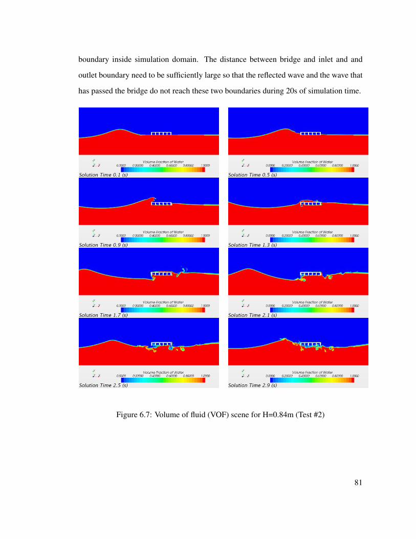
boundary inside simulation domain. The distance between bridge and inlet and and
outlet boundary need to be sufficiently large so that the reflected wave and the wave that
has passed the bridge do not reach these two boundaries during 20s of simulation time.
Figure 6.7: Volume of fluid (VOF) scene for H=0.84m (Test #2)
81
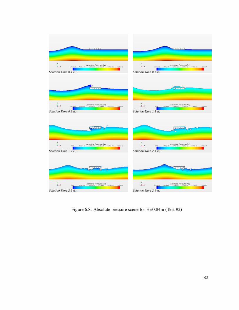
Figure 6.8: Absolute pressure scene for H=0.84m (Test #2)
82

Figure 6.9: Velocity vector scene for H=0.84m (Test #2)
83
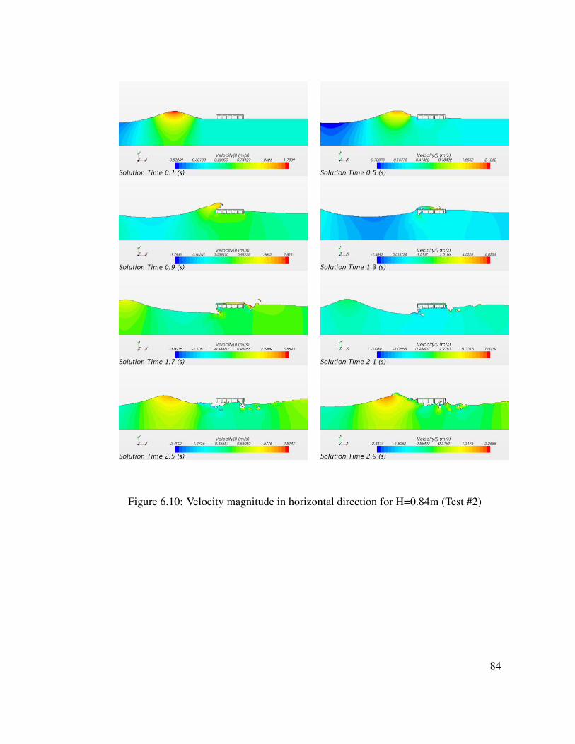
Figure 6.10: Velocity magnitude in horizontal direction for H=0.84m (Test #2)
84
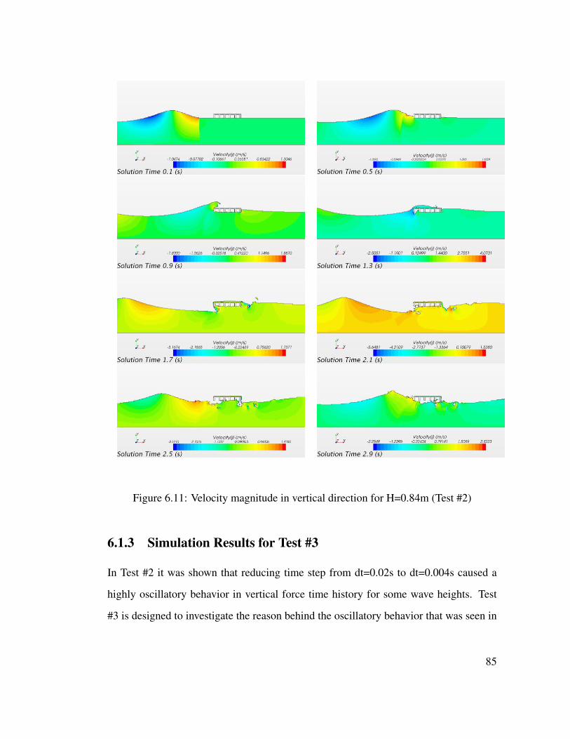
Figure 6.11: Velocity magnitude in vertical direction for H=0.84m (Test #2)
6.1.3 Simulation Results for Test #3
In Test #2 it was shown that reducing time step from dt=0.02s to dt=0.004s caused a
highly oscillatory behavior in vertical force time history for some wave heights. Test
#3 is designed to investigate the reason behind the oscillatory behavior that was seen in
85

vertical force time history as time step was reduced. According to the report from uni-
versity of Florida, air entrapment between bridge girders and diaphragms cause oscil-
latory behavior ( Sheppard and Marin (2009)). How ever this was not verified because
the experimented bridge was made airtight and no experiment was conducted to validate
the theory of air entrapment causing oscillatory behavior in vertical force time histories.
The oscillatory behavior was seen in simulation time histories of vertical forces of Test
#1 but it was amplified as time step reduced to Tp/625 in Test #2.
To confirm this theory, in Test #3, the symmetry plane boundary condition at the
side of simulation domain is replaced by pressure outlet. Pressure outlet boundary will
allow both air and water to exit from the side of simulation domain. This is not a
realistic boundary condition how ever it will allow us to investigate how entrapment of
air influence the shape of both horizontal and vertical force time histories. Simulation
results are plotted in figures 6.12, 6.13, and 6.14. As it is seen both horizontal and
vertical force time history for Test #3 do not show any oscillatory behavior. In addition
since the water and the air both can exit from simulation domain from the side, there is
not that much wave reflection from bridge because the water simply exists the side of
simulation domain instead of reflecting back from bridge. This is shown in figure 6.15.
Comparing to Test #1 which had the same time step as Test #3, it is interesting to note
that allowing both the air and water to move out of simulation domain from the side,
does not seem to increase error in horizontal force predictions. In fact, the maximum
error in horizontal force prediction reduced from 48 percent in Test #1 to 19 percent in
Test #3. This shows that horizontal wave force time histories are not influenced by air
entrapment. It also shows that in Test #1 and Test #2 models excessive air entrapment
happens because when the air is allowed to fully vent out from the side of simulation
domain, horizontal force prediction accuracy became better.
86
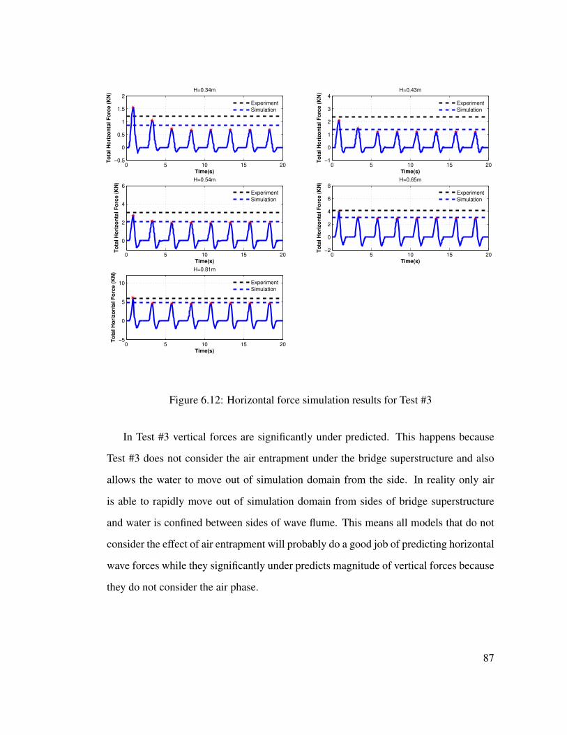
0 5 10 15 20−0.5
0
0.5
1
1.5
2
Time(s)
To
tal
Ho
rizo
nta
l F
orc
e (
KN
)
H=0.34m
Experiment
Simulation
0 5 10 15 20−1
0
1
2
3
4
Time(s)
To
tal
Ho
rizo
nta
l F
orc
e (
KN
)
H=0.43m
Experiment
Simulation
0 5 10 15 20
0
2
4
6
Time(s)
To
tal
Ho
rizo
nta
l F
orc
e (
KN
)
H=0.54m
Experiment
Simulation
0 5 10 15 20−2
0
2
4
6
8
Time(s)
To
tal
Ho
rizo
nta
l F
orc
e (
KN
)
H=0.65m
Experiment
Simulation
0 5 10 15 20−5
0
5
10
Time(s)
To
tal
Ho
rizo
nta
l F
orc
e (
KN
)
H=0.81m
Experiment
Simulation
Figure 6.12: Horizontal force simulation results for Test #3
In Test #3 vertical forces are significantly under predicted. This happens because
Test #3 does not consider the air entrapment under the bridge superstructure and also
allows the water to move out of simulation domain from the side. In reality only air
is able to rapidly move out of simulation domain from sides of bridge superstructure
and water is confined between sides of wave flume. This means all models that do not
consider the effect of air entrapment will probably do a good job of predicting horizontal
wave forces while they significantly under predicts magnitude of vertical forces because
they do not consider the air phase.
87
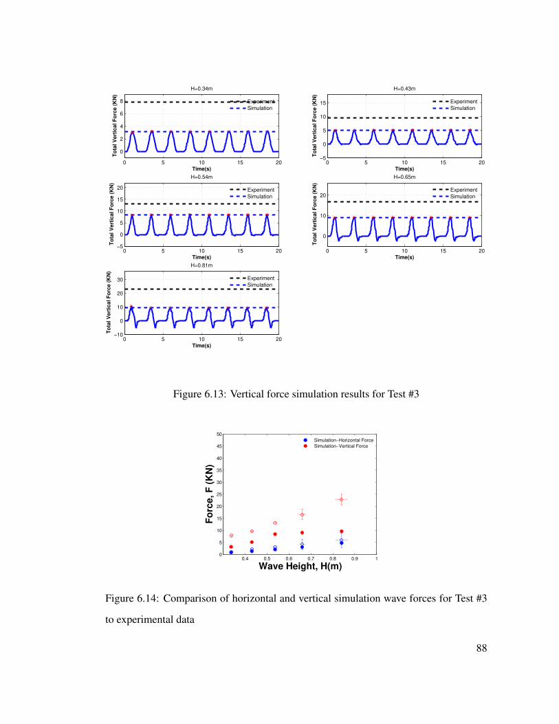
0 5 10 15 20
0
2
4
6
8
Time(s)
To
tal
Ve
rtic
al
Fo
rce
(K
N)
H=0.34m
Experiment
Simulation
0 5 10 15 20−5
0
5
10
15
Time(s)
To
tal
Ve
rtic
al
Fo
rce
(K
N)
H=0.43m
Experiment
Simulation
0 5 10 15 20−5
0
5
10
15
20
Time(s)
To
tal
Ve
rtic
al
Fo
rce
(K
N)
H=0.54m
Experiment
Simulation
0 5 10 15 20
0
10
20
Time(s)
To
tal
Ve
rtic
al
Fo
rce
(K
N)
H=0.65m
Experiment
Simulation
0 5 10 15 20−10
0
10
20
30
Time(s)
To
tal
Ve
rtic
al
Fo
rce
(K
N)
H=0.81m
Experiment
Simulation
Figure 6.13: Vertical force simulation results for Test #3
0.4 0.5 0.6 0.7 0.8 0.9 10
5
10
15
20
25
30
35
40
45
50
Wave Height, H(m)
Fo
rce, F
(K
N)
Simulation−Horizontal Force
Simulation−Vertical Force
Figure 6.14: Comparison of horizontal and vertical simulation wave forces for Test #3
to experimental data
88
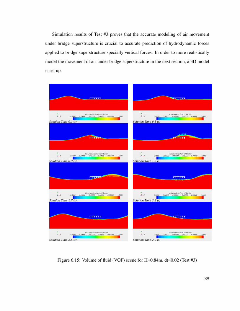
Simulation results of Test #3 proves that the accurate modeling of air movement
under bridge superstructure is crucial to accurate prediction of hydrodynamic forces
applied to bridge superstructure specially vertical forces. In order to more realistically
model the movement of air under bridge superstructure in the next section, a 3D model
is set up.
Figure 6.15: Volume of fluid (VOF) scene for H=0.84m, dt=0.02 (Test #3)
89
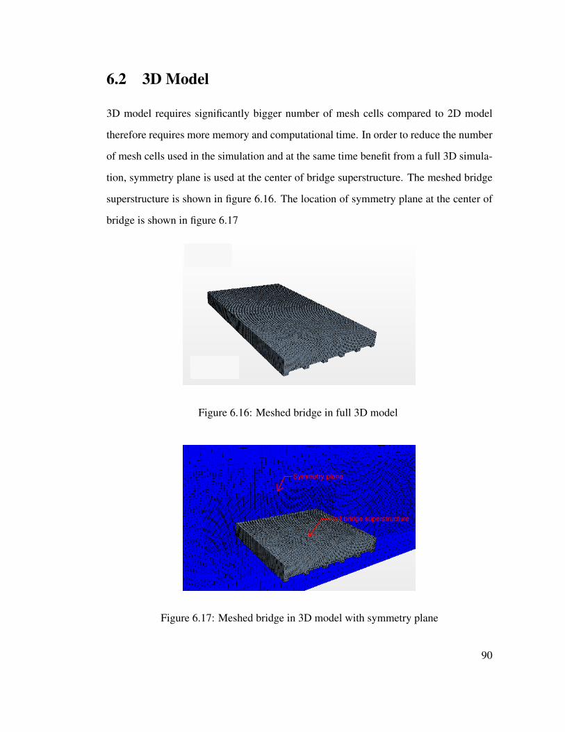
6.2 3D Model
3D model requires significantly bigger number of mesh cells compared to 2D model
therefore requires more memory and computational time. In order to reduce the number
of mesh cells used in the simulation and at the same time benefit from a full 3D simula-
tion, symmetry plane is used at the center of bridge superstructure. The meshed bridge
superstructure is shown in figure 6.16. The location of symmetry plane at the center of
bridge is shown in figure 6.17
Figure 6.16: Meshed bridge in full 3D model
Symmetry plane
Half bridge superstructure
Figure 6.17: Meshed bridge in 3D model with symmetry plane
90
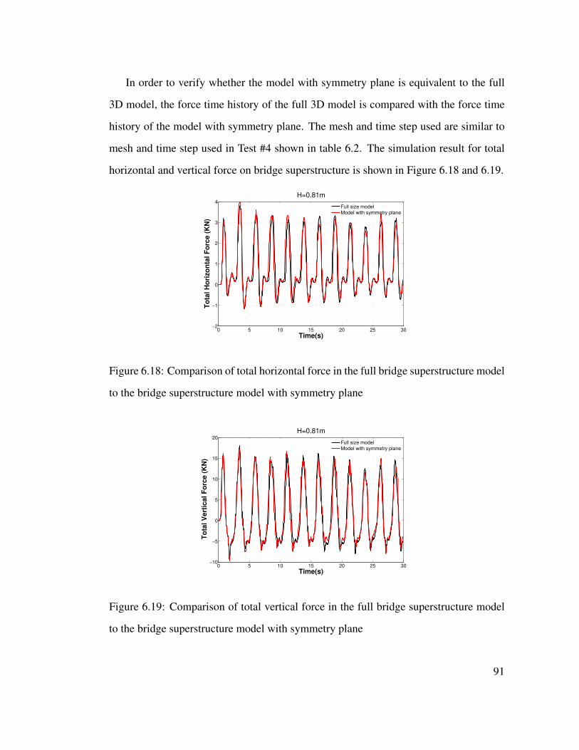
In order to verify whether the model with symmetry plane is equivalent to the full
3D model, the force time history of the full 3D model is compared with the force time
history of the model with symmetry plane. The mesh and time step used are similar to
mesh and time step used in Test #4 shown in table 6.2. The simulation result for total
horizontal and vertical force on bridge superstructure is shown in Figure 6.18 and 6.19.
0 5 10 15 20 25 30−2
−1
0
1
2
3
4
Time(s)
To
tal
Ho
rizo
nta
l F
orc
e (
KN
)
H=0.81m
Full size model
Model with symmetry plane
Figure 6.18: Comparison of total horizontal force in the full bridge superstructure model
to the bridge superstructure model with symmetry plane
0 5 10 15 20 25 30−10
−5
0
5
10
15
20
Time(s)
To
tal
Ve
rtic
al
Fo
rce
(K
N)
H=0.81m
Full size model
Model with symmetry plane
Figure 6.19: Comparison of total vertical force in the full bridge superstructure model
to the bridge superstructure model with symmetry plane
91
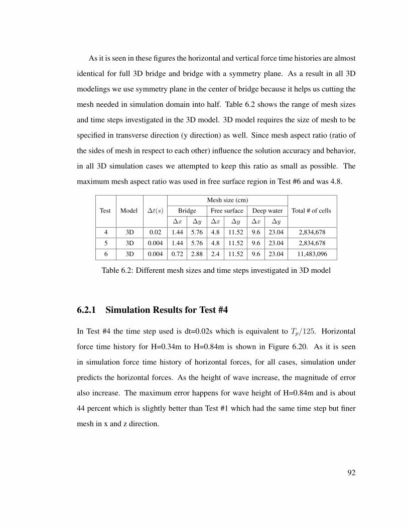
As it is seen in these figures the horizontal and vertical force time histories are almost
identical for full 3D bridge and bridge with a symmetry plane. As a result in all 3D
modelings we use symmetry plane in the center of bridge because it helps us cutting the
mesh needed in simulation domain into half. Table 6.2 shows the range of mesh sizes
and time steps investigated in the 3D model. 3D model requires the size of mesh to be
specified in transverse direction (y direction) as well. Since mesh aspect ratio (ratio of
the sides of mesh in respect to each other) influence the solution accuracy and behavior,
in all 3D simulation cases we attempted to keep this ratio as small as possible. The
maximum mesh aspect ratio was used in free surface region in Test #6 and was 4.8.
Test Model ∆t(s)
Mesh size (cm)
Total # of cellsBridge Free surface Deep water
∆x ∆y ∆x ∆y ∆x ∆y
4 3D 0.02 1.44 5.76 4.8 11.52 9.6 23.04 2,834,678
5 3D 0.004 1.44 5.76 4.8 11.52 9.6 23.04 2,834,678
6 3D 0.004 0.72 2.88 2.4 11.52 9.6 23.04 11,483,096
Table 6.2: Different mesh sizes and time steps investigated in 3D model
6.2.1 Simulation Results for Test #4
In Test #4 the time step used is dt=0.02s which is equivalent to Tp/125. Horizontal
force time history for H=0.34m to H=0.84m is shown in Figure 6.20. As it is seen
in simulation force time history of horizontal forces, for all cases, simulation under
predicts the horizontal forces. As the height of wave increase, the magnitude of error
also increase. The maximum error happens for wave height of H=0.84m and is about
44 percent which is slightly better than Test #1 which had the same time step but finer
mesh in x and z direction.
92
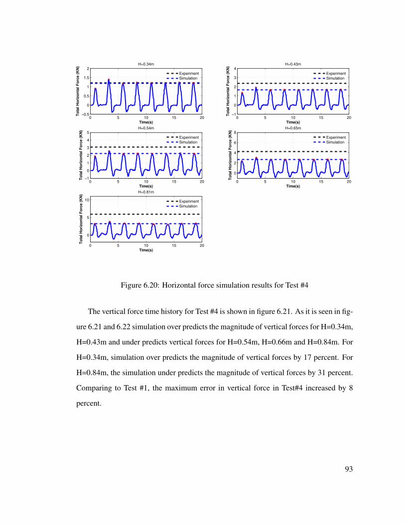
0 5 10 15 20−0.5
0
0.5
1
1.5
2
Time(s)
To
tal
Ho
rizo
nta
l F
orc
e (
KN
)
H=0.34m
Experiment
Simulation
0 5 10 15 20−1
0
1
2
3
4
Time(s)
To
tal
Ho
rizo
nta
l F
orc
e (
KN
)
H=0.43m
Experiment
Simulation
0 5 10 15 20−1
0
1
2
3
4
5
Time(s)
To
tal
Ho
rizo
nta
l F
orc
e (
KN
)
H=0.54m
Experiment
Simulation
0 5 10 15 20
0
2
4
6
8
Time(s)
To
tal
Ho
rizo
nta
l F
orc
e (
KN
)
H=0.65m
Experiment
Simulation
0 5 10 15 20
0
5
10
Time(s)
To
tal
Ho
rizo
nta
l F
orc
e (
KN
)
H=0.81m
Experiment
Simulation
Figure 6.20: Horizontal force simulation results for Test #4
The vertical force time history for Test #4 is shown in figure 6.21. As it is seen in fig-
ure 6.21 and 6.22 simulation over predicts the magnitude of vertical forces for H=0.34m,
H=0.43m and under predicts vertical forces for H=0.54m, H=0.66m and H=0.84m. For
H=0.34m, simulation over predicts the magnitude of vertical forces by 17 percent. For
H=0.84m, the simulation under predicts the magnitude of vertical forces by 31 percent.
Comparing to Test #1, the maximum error in vertical force in Test#4 increased by 8
percent.
93
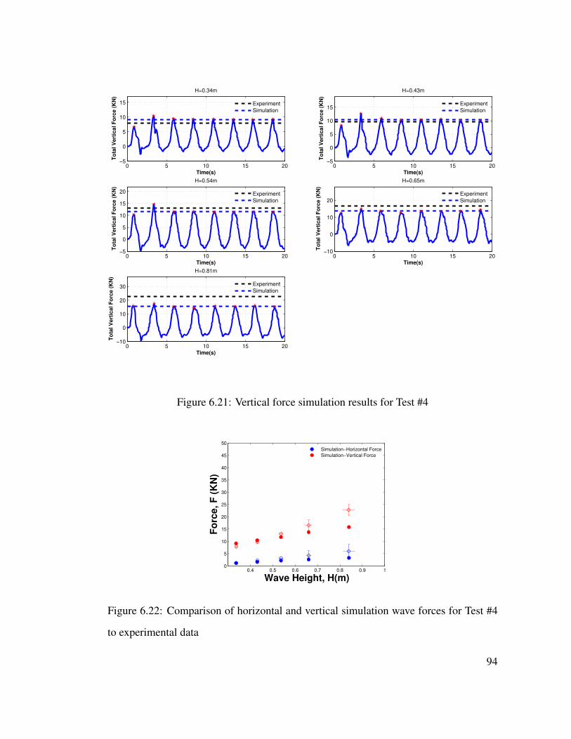
0 5 10 15 20−5
0
5
10
15
Time(s)
To
tal
Ve
rtic
al
Fo
rce
(K
N)
H=0.34m
Experiment
Simulation
0 5 10 15 20−5
0
5
10
15
Time(s)
To
tal
Ve
rtic
al
Fo
rce
(K
N)
H=0.43m
Experiment
Simulation
0 5 10 15 20−5
0
5
10
15
20
Time(s)
To
tal
Ve
rtic
al
Fo
rce
(K
N)
H=0.54m
Experiment
Simulation
0 5 10 15 20−10
0
10
20
Time(s)
To
tal
Ve
rtic
al
Fo
rce
(K
N)
H=0.65m
Experiment
Simulation
0 5 10 15 20−10
0
10
20
30
Time(s)
To
tal
Ve
rtic
al
Fo
rce
(K
N)
H=0.81m
Experiment
Simulation
Figure 6.21: Vertical force simulation results for Test #4
0.4 0.5 0.6 0.7 0.8 0.9 10
5
10
15
20
25
30
35
40
45
50
Wave Height, H(m)
Fo
rce, F
(K
N)
Simulation−Horizontal Force
Simulation−Vertical Force
Figure 6.22: Comparison of horizontal and vertical simulation wave forces for Test #4
to experimental data
94

6.2.2 Simulation Results for Test #5
In Test #5 the time step is reduced to dt=0.004s which is equivalent to Tp/625. This is
done because in 2D model it was shown that reduction of time step improved the accu-
racy of horizontal force predictions. Mesh that is used in Test #5 is exactly the same as
mesh used in Test #4. Horizontal force time history for H=0.34m to H=0.84m is shown
in Figure 6.23. As the height of wave increase, the magnitude of error also increase. The
maximum error happens for wave height of H=0.84m and is about 27 percent which is
better than Test #4 which had maximum error of 44 percent. The vertical force time his-
tory is shown in figure 6.24. As it is seen in figure 6.24 and 6.25 simulation over predicts
the magnitude of vertical forces for H=0.34m, H=0.43m, H=0.54m, and H=0.66m and
under predicts the magnitude of vertical force for H=0.84m. For H=0.34m, simulation
over predicts the magnitude vertical force by 60 percent. For H=0.84m, the simulation
under predicts the magnitude of vertical force by 17 percent. Comparing to Test #4
vertical force time history results, Test #5 model does a better job of predicting vertical
wave forces for H=0.84m. The error in prediction of wave forces for H=0.34m increased
from 17 percent to 60 percent. Comparing to Test #2 which had the same time step size,
Test #5 predicts both horizontal and vertical forces with better accuracy. Compared to
Test #2, the error in horizontal force prediction reduced by 10 percent and the error in
vertical force prediction reduced by 33 percent. Looking into behavior of vertical force
time history for H=0.34m, H=0.43m and H=0.54m we witness some oscillatory behav-
ior similar to Test #2 results. Test #3 simulations showed that the oscillatory behavior
in vertical force time history is the result of air entrapment between bridge girders and
diaphragms. Test #5 time histories for H=0.34m, H=0.43m and H=0.54m show a similar
behavior to Test #2 except for Test #5 oscillations having smaller amplitude than Test
#2.
95
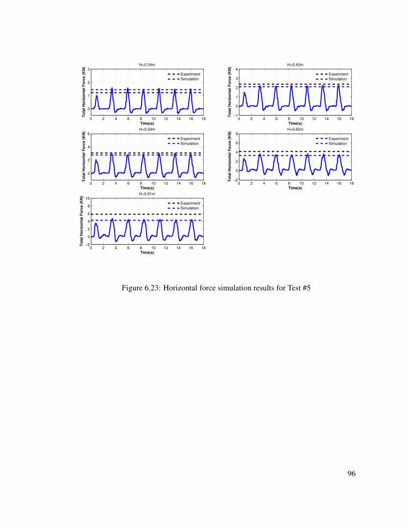
0 2 4 6 8 10 12 14 16 18
0
1
2
3
Time(s)
To
tal
Ho
rizo
nta
l F
orc
e (
KN
)
H=0.34m
Experiment
Simulation
0 2 4 6 8 10 12 14 16 18−1
0
1
2
3
4
Time(s)
To
tal
Ho
rizo
nta
l F
orc
e (
KN
)
H=0.43m
Experiment
Simulation
0 2 4 6 8 10 12 14 16 18
0
2
4
6
Time(s)
To
tal
Ho
rizo
nta
l F
orc
e (
KN
)
H=0.54m
Experiment
Simulation
0 2 4 6 8 10 12 14 16 18−2
0
2
4
6
8
Time(s)
To
tal
Ho
rizo
nta
l F
orc
e (
KN
)
H=0.65m
Experiment
Simulation
0 2 4 6 8 10 12 14 16 18−2
0
2
4
6
8
10
Time(s)
To
tal
Ho
rizo
nta
l F
orc
e (
KN
)
H=0.81m
Experiment
Simulation
Figure 6.23: Horizontal force simulation results for Test #5
96
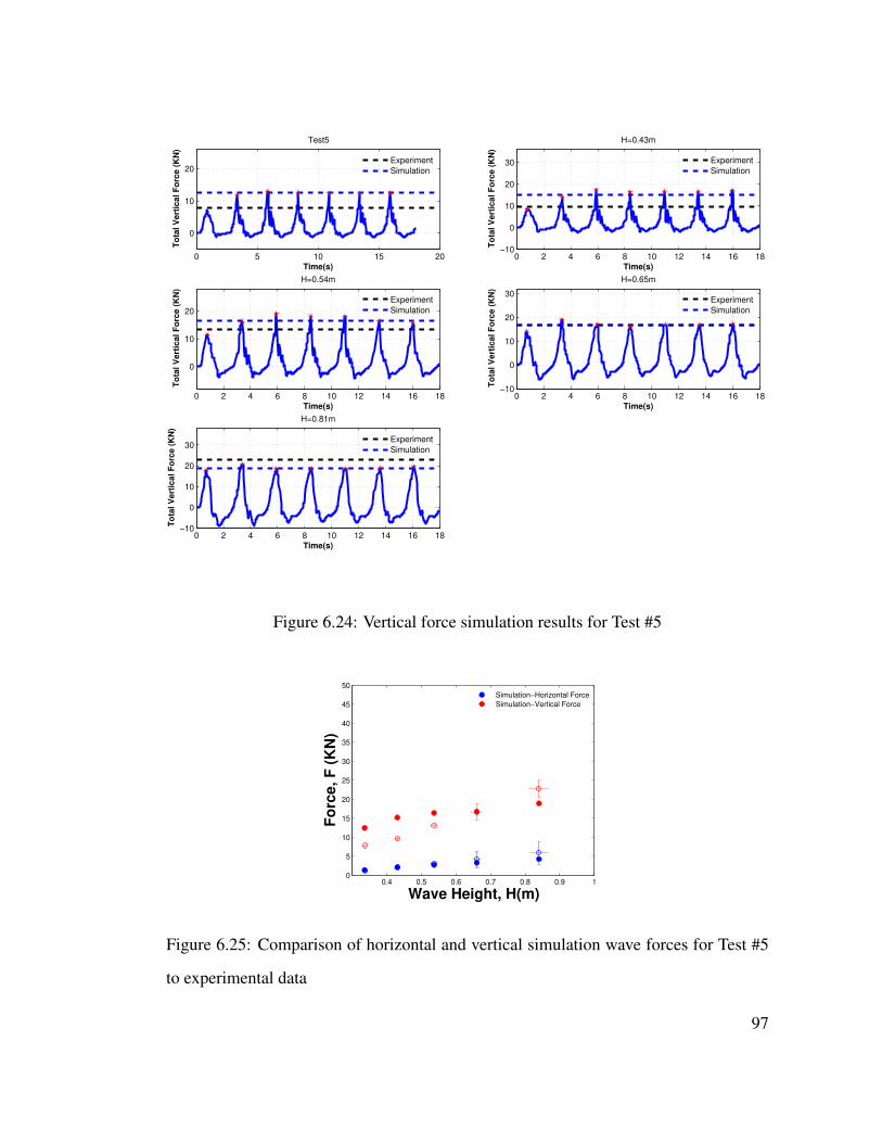
0 5 10 15 20
0
10
20
Time(s)
To
tal
Ve
rtic
al
Fo
rce
(K
N)
Test5
Experiment
Simulation
0 2 4 6 8 10 12 14 16 18−10
0
10
20
30
Time(s)
To
tal
Ve
rtic
al
Fo
rce
(K
N)
H=0.43m
Experiment
Simulation
0 2 4 6 8 10 12 14 16 18
0
10
20
Time(s)
To
tal
Ve
rtic
al
Fo
rce
(K
N)
H=0.54m
Experiment
Simulation
0 2 4 6 8 10 12 14 16 18−10
0
10
20
30
Time(s)
To
tal
Ve
rtic
al
Fo
rce
(K
N)
H=0.65m
Experiment
Simulation
0 2 4 6 8 10 12 14 16 18−10
0
10
20
30
Time(s)
To
tal
Ve
rtic
al
Fo
rce
(K
N)
H=0.81m
Experiment
Simulation
Figure 6.24: Vertical force simulation results for Test #5
0.4 0.5 0.6 0.7 0.8 0.9 10
5
10
15
20
25
30
35
40
45
50
Wave Height, H(m)
Fo
rce, F
(K
N)
Simulation−Horizontal Force
Simulation−Vertical Force
Figure 6.25: Comparison of horizontal and vertical simulation wave forces for Test #5
to experimental data
97
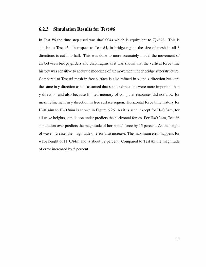
6.2.3 Simulation Results for Test #6
In Test #6 the time step used was dt=0.004s which is equivalent to Tp/625. This is
similar to Test #5. In respect to Test #5, in bridge region the size of mesh in all 3
directions is cut into half. This was done to more accurately model the movement of
air between bridge girders and diaphragms as it was shown that the vertical force time
history was sensitive to accurate modeling of air movement under bridge superstructure.
Compared to Test #5 mesh in free surface is also refined in x and z direction but kept
the same in y direction as it is assumed that x and z directions were more important than
y direction and also because limited memory of computer resources did not alow for
mesh refinement in y direction in free surface region. Horizontal force time history for
H=0.34m to H=0.84m is shown in Figure 6.26. As it is seen, except for H=0.34m, for
all wave heights, simulation under predicts the horizontal forces. For H=0.34m, Test #6
simulation over predicts the magnitude of horizontal force by 15 percent. As the height
of wave increase, the magnitude of error also increase. The maximum error happens for
wave height of H=0.84m and is about 32 percent. Compared to Test #5 the magnitude
of error increased by 5 percent.
98
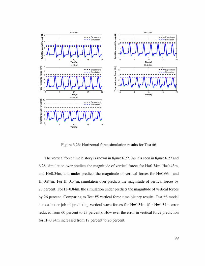
0 5 10 15 20
0
1
2
3
Time(s)
To
tal
Ho
rizo
nta
l F
orc
e (
KN
)
H=0.34m
Experiment
Simulation
0 5 10 15 20−1
0
1
2
3
4
Time(s)
To
tal
Ho
rizo
nta
l F
orc
e (
KN
)
H=0.43m
Experiment
Simulation
0 5 10 15 20−1
0
1
2
3
4
5
Time(s)
To
tal
Ho
rizo
nta
l F
orc
e (
KN
)
H=0.54m
Experiment
Simulation
0 5 10 15 20−2
0
2
4
6
Time(s)
To
tal
Ho
rizo
nta
l F
orc
e (
KN
)
H=0.65m
Experiment
Simulation
0 5 10 15 20−2
0
2
4
6
8
10
Time(s)
To
tal
Ho
rizo
nta
l F
orc
e (
KN
)
H=0.81m
Experiment
Simulation
Figure 6.26: Horizontal force simulation results for Test #6
The vertical force time history is shown in figure 6.27. As it is seen in figure 6.27 and
6.28, simulation over predicts the magnitude of vertical forces for H=0.34m, H=0.43m,
and H=0.54m, and under predicts the magnitude of vertical forces for H=0.66m and
H=0.84m. For H=0.34m, simulation over predicts the magnitude of vertical forces by
23 percent. For H=0.84m, the simulation under predicts the magnitude of vertical forces
by 26 percent. Comparing to Test #5 vertical force time history results, Test #6 model
does a better job of predicting vertical wave forces for H=0.34m (for H=0.34m error
reduced from 60 percent to 23 percent). How ever the error in vertical force prediction
for H=0.84m increased from 17 percent to 26 percent.
99
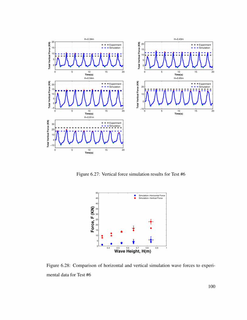
0 5 10 15 20
0
5
10
15
20
Time(s)
To
tal
Ve
rtic
al
Fo
rce
(K
N)
H=0.34m
Experiment
Simulation
0 5 10 15 20
0
5
10
15
20
Time(s)
To
tal
Ve
rtic
al
Fo
rce
(K
N)
H=0.43m
Experiment
Simulation
0 5 10 15 20
−5
0
5
10
15
20
Time(s)
To
tal
Ve
rtic
al
Fo
rce
(K
N)
H=0.54m
Experiment
Simulation
0 5 10 15 20−10
0
10
20
Time(s)
To
tal
Ve
rtic
al
Fo
rce
(K
N)
H=0.65m
Experiment
Simulation
0 5 10 15 20
−10
0
10
20
30
Time(s)
To
tal
Ve
rtic
al
Fo
rce
(K
N)
H=0.81m
Experiment
Simulation
Figure 6.27: Vertical force simulation results for Test #6
0.4 0.5 0.6 0.7 0.8 0.9 10
5
10
15
20
25
30
35
40
45
50
Wave Height, H(m)
Fo
rce, F
(K
N)
Simulation−Horizontal Force
Simulation−Vertical Force
Figure 6.28: Comparison of horizontal and vertical simulation wave forces to experi-
mental data for Test #6
100
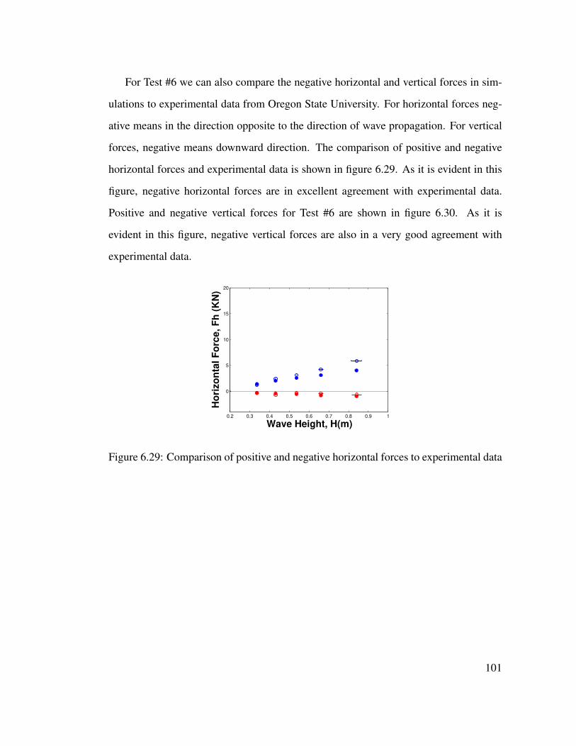
For Test #6 we can also compare the negative horizontal and vertical forces in sim-
ulations to experimental data from Oregon State University. For horizontal forces neg-
ative means in the direction opposite to the direction of wave propagation. For vertical
forces, negative means downward direction. The comparison of positive and negative
horizontal forces and experimental data is shown in figure 6.29. As it is evident in this
figure, negative horizontal forces are in excellent agreement with experimental data.
Positive and negative vertical forces for Test #6 are shown in figure 6.30. As it is
evident in this figure, negative vertical forces are also in a very good agreement with
experimental data.
0.2 0.3 0.4 0.5 0.6 0.7 0.8 0.9 1
0
5
10
15
20
Wave Height, H(m)
Ho
rizo
nta
l F
orc
e, F
h (
KN
)
Figure 6.29: Comparison of positive and negative horizontal forces to experimental data
101
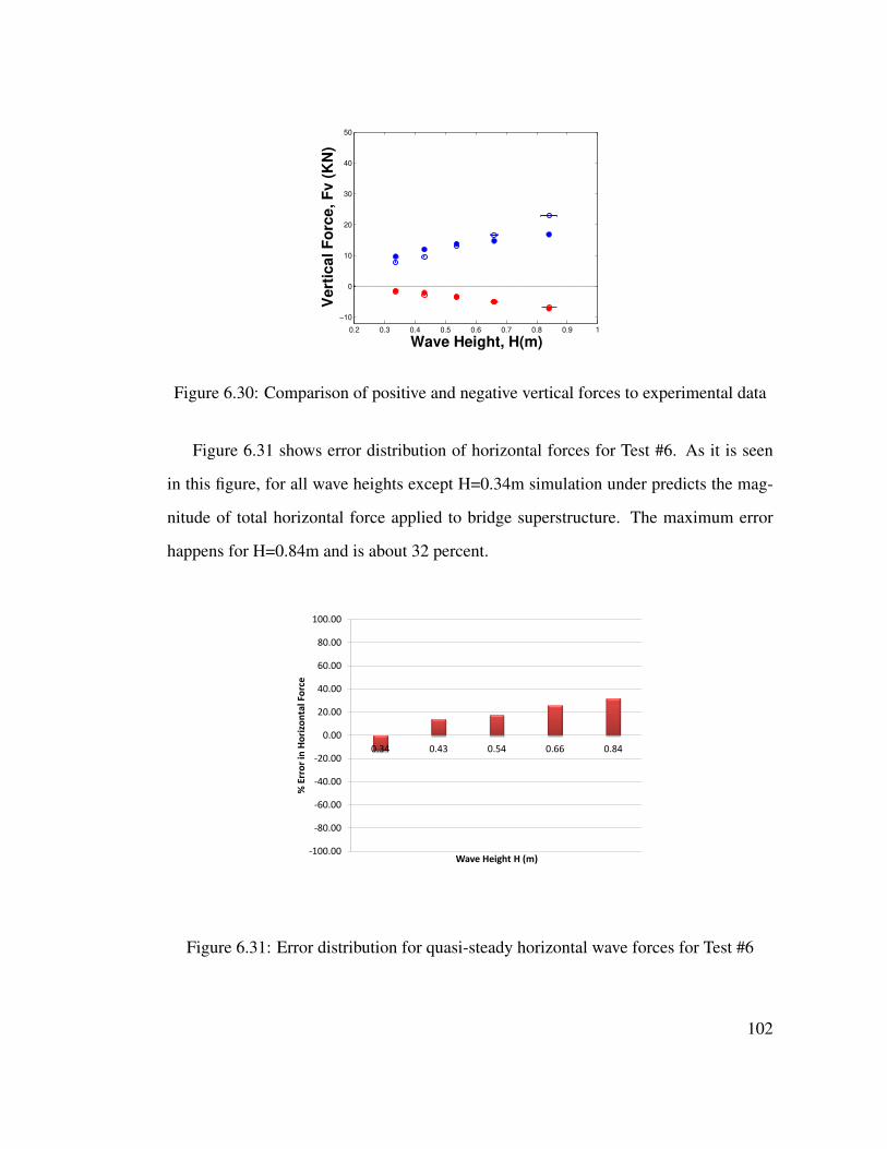
0.2 0.3 0.4 0.5 0.6 0.7 0.8 0.9 1
−10
0
10
20
30
40
50
Wave Height, H(m)V
ert
ical F
orc
e, F
v (
KN
)
Figure 6.30: Comparison of positive and negative vertical forces to experimental data
Figure 6.31 shows error distribution of horizontal forces for Test #6. As it is seen
in this figure, for all wave heights except H=0.34m simulation under predicts the mag-
nitude of total horizontal force applied to bridge superstructure. The maximum error
happens for H=0.84m and is about 32 percent.
-100.00
-80.00
-60.00
-40.00
-20.00
0.00
20.00
40.00
60.00
80.00
100.00
0.34 0.43 0.54 0.66 0.84
% E
rro
r in
Ho
rizo
nta
l Fo
rce
Wave Height H (m)
Figure 6.31: Error distribution for quasi-steady horizontal wave forces for Test #6
102
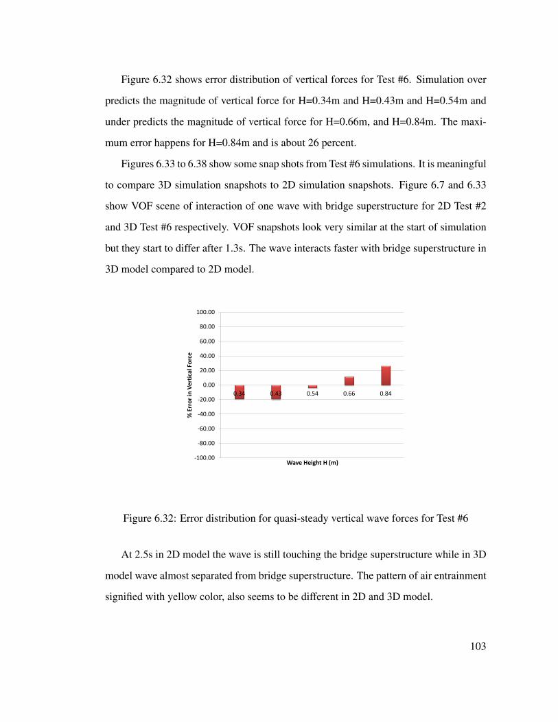
Figure 6.32 shows error distribution of vertical forces for Test #6. Simulation over
predicts the magnitude of vertical force for H=0.34m and H=0.43m and H=0.54m and
under predicts the magnitude of vertical force for H=0.66m, and H=0.84m. The maxi-
mum error happens for H=0.84m and is about 26 percent.
Figures 6.33 to 6.38 show some snap shots from Test #6 simulations. It is meaningful
to compare 3D simulation snapshots to 2D simulation snapshots. Figure 6.7 and 6.33
show VOF scene of interaction of one wave with bridge superstructure for 2D Test #2
and 3D Test #6 respectively. VOF snapshots look very similar at the start of simulation
but they start to differ after 1.3s. The wave interacts faster with bridge superstructure in
3D model compared to 2D model.
-100.00
-80.00
-60.00
-40.00
-20.00
0.00
20.00
40.00
60.00
80.00
100.00
0.34 0.43 0.54 0.66 0.84
% E
rro
r in
Ve
rtic
al
Fo
rce
Wave Height H (m)
Figure 6.32: Error distribution for quasi-steady vertical wave forces for Test #6
At 2.5s in 2D model the wave is still touching the bridge superstructure while in 3D
model wave almost separated from bridge superstructure. The pattern of air entrainment
signified with yellow color, also seems to be different in 2D and 3D model.
103
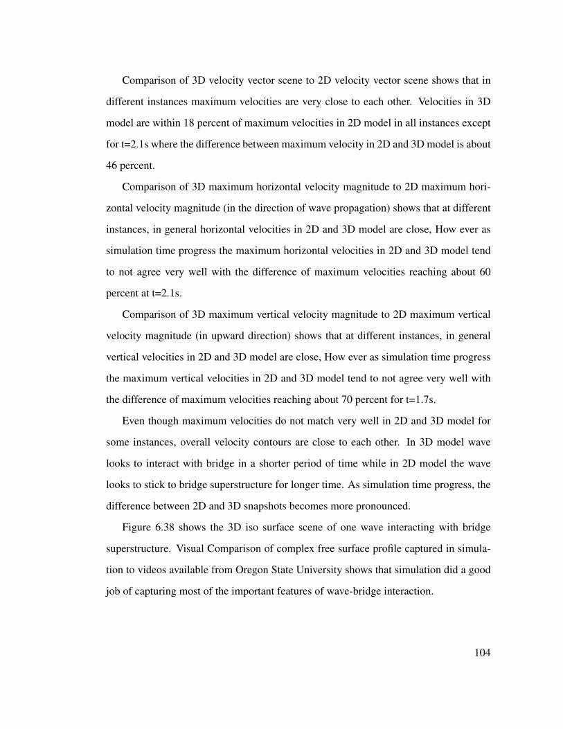
Comparison of 3D velocity vector scene to 2D velocity vector scene shows that in
different instances maximum velocities are very close to each other. Velocities in 3D
model are within 18 percent of maximum velocities in 2D model in all instances except
for t=2.1s where the difference between maximum velocity in 2D and 3D model is about
46 percent.
Comparison of 3D maximum horizontal velocity magnitude to 2D maximum hori-
zontal velocity magnitude (in the direction of wave propagation) shows that at different
instances, in general horizontal velocities in 2D and 3D model are close, How ever as
simulation time progress the maximum horizontal velocities in 2D and 3D model tend
to not agree very well with the difference of maximum velocities reaching about 60
percent at t=2.1s.
Comparison of 3D maximum vertical velocity magnitude to 2D maximum vertical
velocity magnitude (in upward direction) shows that at different instances, in general
vertical velocities in 2D and 3D model are close, How ever as simulation time progress
the maximum vertical velocities in 2D and 3D model tend to not agree very well with
the difference of maximum velocities reaching about 70 percent for t=1.7s.
Even though maximum velocities do not match very well in 2D and 3D model for
some instances, overall velocity contours are close to each other. In 3D model wave
looks to interact with bridge in a shorter period of time while in 2D model the wave
looks to stick to bridge superstructure for longer time. As simulation time progress, the
difference between 2D and 3D snapshots becomes more pronounced.
Figure 6.38 shows the 3D iso surface scene of one wave interacting with bridge
superstructure. Visual Comparison of complex free surface profile captured in simula-
tion to videos available from Oregon State University shows that simulation did a good
job of capturing most of the important features of wave-bridge interaction.
104
Figure 6.33: Volume of fluid (VOF) scene for H=0.84m (Test #6)
105
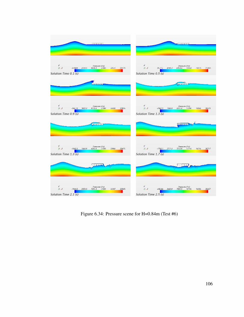
Figure 6.34: Pressure scene for H=0.84m (Test #6)
106

Figure 6.35: Velocity vector scene for H=0.84m (Test #6)
107
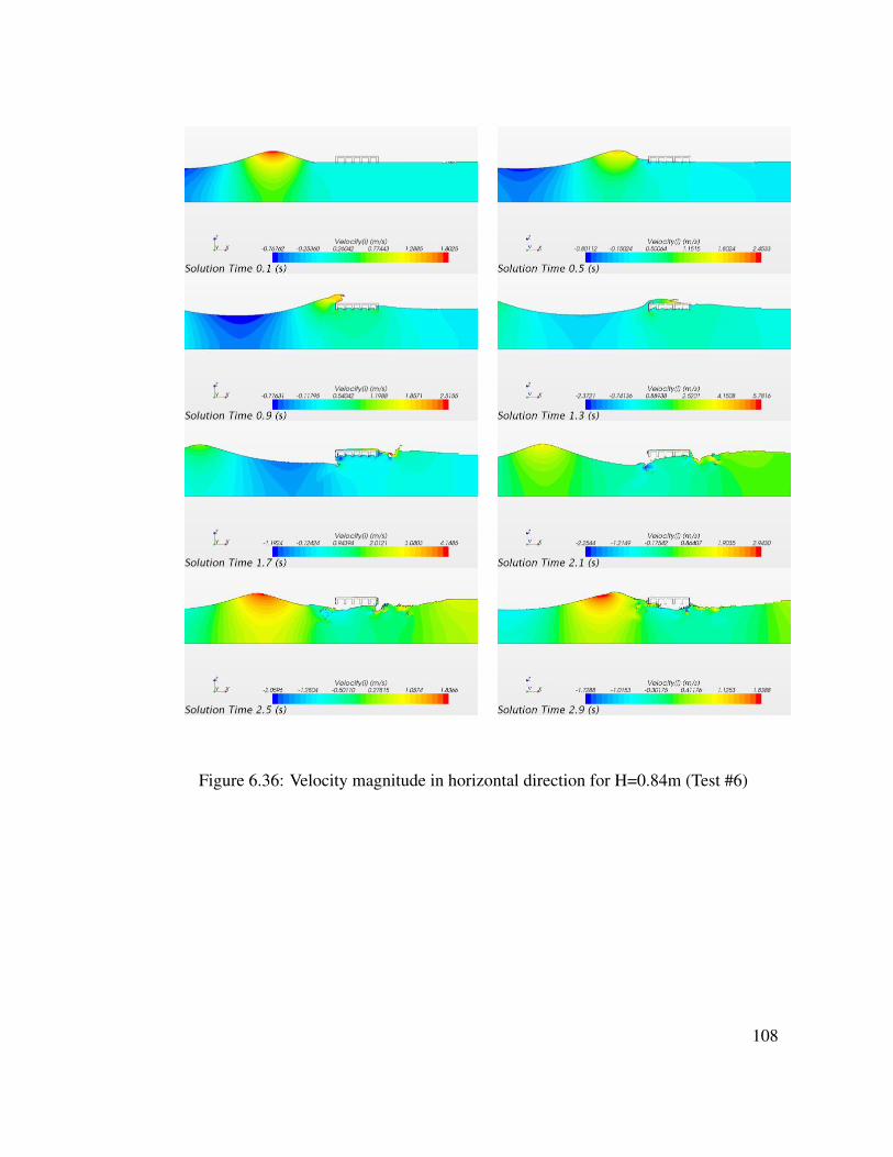
Figure 6.36: Velocity magnitude in horizontal direction for H=0.84m (Test #6)
108
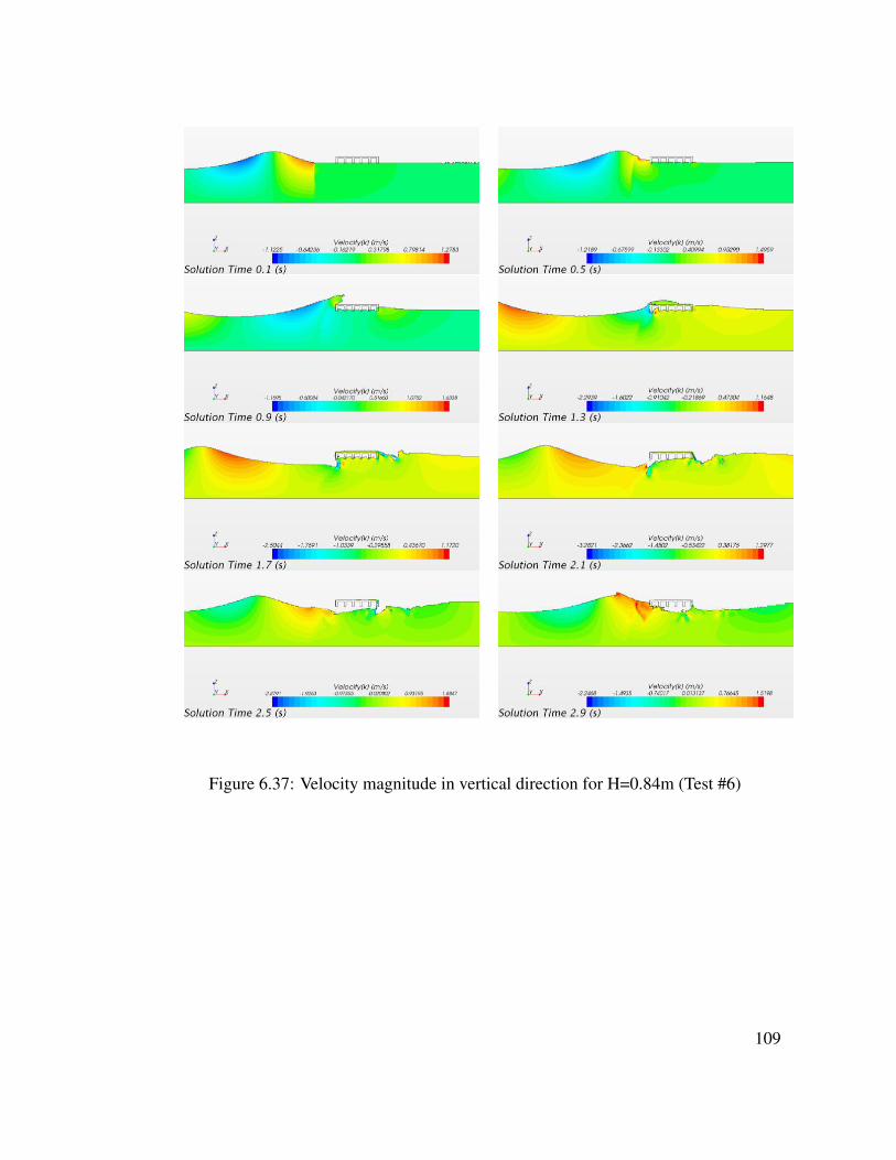
Figure 6.37: Velocity magnitude in vertical direction for H=0.84m (Test #6)
109
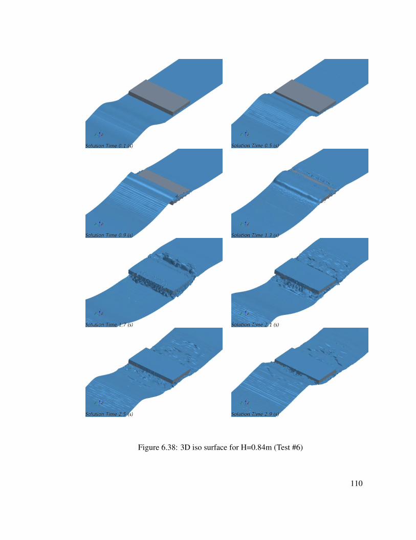
Figure 6.38: 3D iso surface for H=0.84m (Test #6)
110
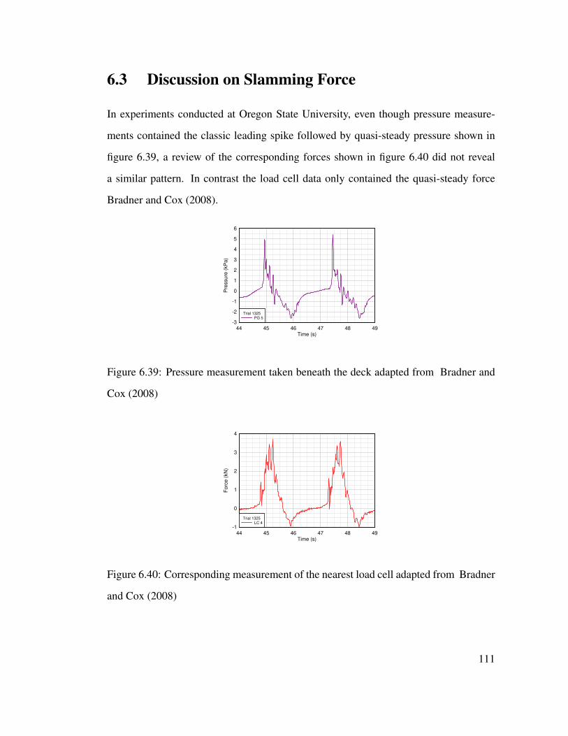
6.3 Discussion on Slamming Force
In experiments conducted at Oregon State University, even though pressure measure-
ments contained the classic leading spike followed by quasi-steady pressure shown in
figure 6.39, a review of the corresponding forces shown in figure 6.40 did not reveal
a similar pattern. In contrast the load cell data only contained the quasi-steady force
Bradner and Cox (2008).
Time (s)
Pre
ssu
re (
kP
a)
44 45 46 47 48 49-3
-2
-1
0
1
2
3
4
5
6
Trial 1325PG 5
4
Figure 6.39: Pressure measurement taken beneath the deck adapted from Bradner and
Cox (2008)
Time (s)
Fo
rce
(kN
)
44 45 46 47 48 49-1
0
1
2
3
4
Trial 1325LC 4
Figure 6.40: Corresponding measurement of the nearest load cell adapted from Bradner
and Cox (2008)
111
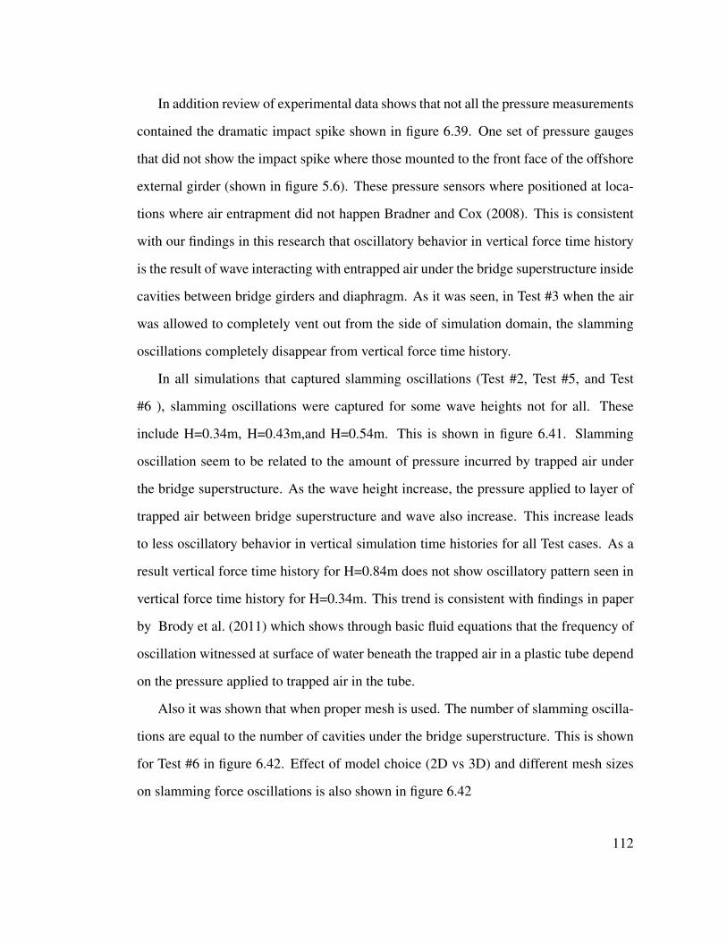
In addition review of experimental data shows that not all the pressure measurements
contained the dramatic impact spike shown in figure 6.39. One set of pressure gauges
that did not show the impact spike where those mounted to the front face of the offshore
external girder (shown in figure 5.6). These pressure sensors where positioned at loca-
tions where air entrapment did not happen Bradner and Cox (2008). This is consistent
with our findings in this research that oscillatory behavior in vertical force time history
is the result of wave interacting with entrapped air under the bridge superstructure inside
cavities between bridge girders and diaphragm. As it was seen, in Test #3 when the air
was allowed to completely vent out from the side of simulation domain, the slamming
oscillations completely disappear from vertical force time history.
In all simulations that captured slamming oscillations (Test #2, Test #5, and Test
#6 ), slamming oscillations were captured for some wave heights not for all. These
include H=0.34m, H=0.43m,and H=0.54m. This is shown in figure 6.41. Slamming
oscillation seem to be related to the amount of pressure incurred by trapped air under
the bridge superstructure. As the wave height increase, the pressure applied to layer of
trapped air between bridge superstructure and wave also increase. This increase leads
to less oscillatory behavior in vertical simulation time histories for all Test cases. As a
result vertical force time history for H=0.84m does not show oscillatory pattern seen in
vertical force time history for H=0.34m. This trend is consistent with findings in paper
by Brody et al. (2011) which shows through basic fluid equations that the frequency of
oscillation witnessed at surface of water beneath the trapped air in a plastic tube depend
on the pressure applied to trapped air in the tube.
Also it was shown that when proper mesh is used. The number of slamming oscilla-
tions are equal to the number of cavities under the bridge superstructure. This is shown
for Test #6 in figure 6.42. Effect of model choice (2D vs 3D) and different mesh sizes
on slamming force oscillations is also shown in figure 6.42
112
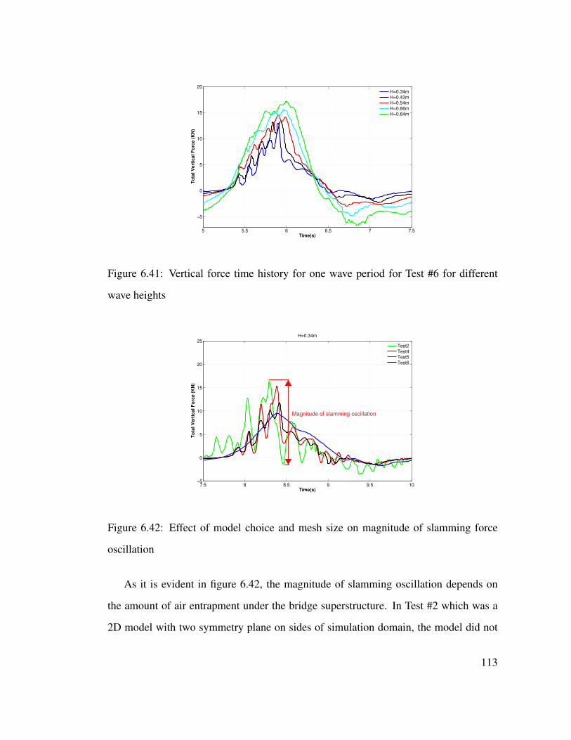
5 5.5 6 6.5 7 7.5
−5
0
5
10
15
20
Time(s)
To
tal
Vert
ical
Fo
rce (
KN
)
H=0.34m
H=0.43m
H=0.54m
H=0.66m
H=0.84m
Figure 6.41: Vertical force time history for one wave period for Test #6 for different
wave heights
7.5 8 8.5 9 9.5 10−5
0
5
10
15
20
25
Time(s)
To
tal V
ert
ical F
orc
e (
KN
)
H=0.34m
Test2
Test4Test5
Test6
Magnitude of slamming oscillation
Figure 6.42: Effect of model choice and mesh size on magnitude of slamming force
oscillation
As it is evident in figure 6.42, the magnitude of slamming oscillation depends on
the amount of air entrapment under the bridge superstructure. In Test #2 which was a
2D model with two symmetry plane on sides of simulation domain, the model did not
113
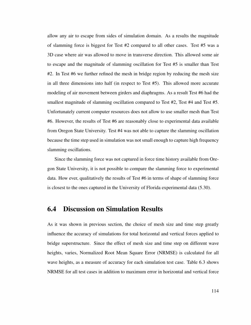
allow any air to escape from sides of simulation domain. As a results the magnitude
of slamming force is biggest for Test #2 compared to all other cases. Test #5 was a
3D case where air was allowed to move in transverse direction. This allowed some air
to escape and the magnitude of slamming oscillation for Test #5 is smaller than Test
#2. In Test #6 we further refined the mesh in bridge region by reducing the mesh size
in all three dimensions into half (in respect to Test #5). This allowed more accurate
modeling of air movement between girders and diaphragms. As a result Test #6 had the
smallest magnitude of slamming oscillation compared to Test #2, Test #4 and Test #5.
Unfortunately current computer resources does not allow to use smaller mesh than Test
#6. However, the results of Test #6 are reasonably close to experimental data available
from Oregon State University. Test #4 was not able to capture the slamming oscillation
because the time step used in simulation was not small enough to capture high frequency
slamming oscillations.
Since the slamming force was not captured in force time history available from Ore-
gon State University, it is not possible to compare the slamming force to experimental
data. How ever, qualitatively the results of Test #6 in terms of shape of slamming force
is closest to the ones captured in the University of Florida experimental data (5.30).
6.4 Discussion on Simulation Results
As it was shown in previous section, the choice of mesh size and time step greatly
influence the accuracy of simulations for total horizontal and vertical forces applied to
bridge superstructure. Since the effect of mesh size and time step on different wave
heights, varies, Normalized Root Mean Square Error (NRMSE) is calculated for all
wave heights, as a measure of accuracy for each simulation test case. Table 6.3 shows
NRMSE for all test cases in addition to maximum error in horizontal and vertical force
114
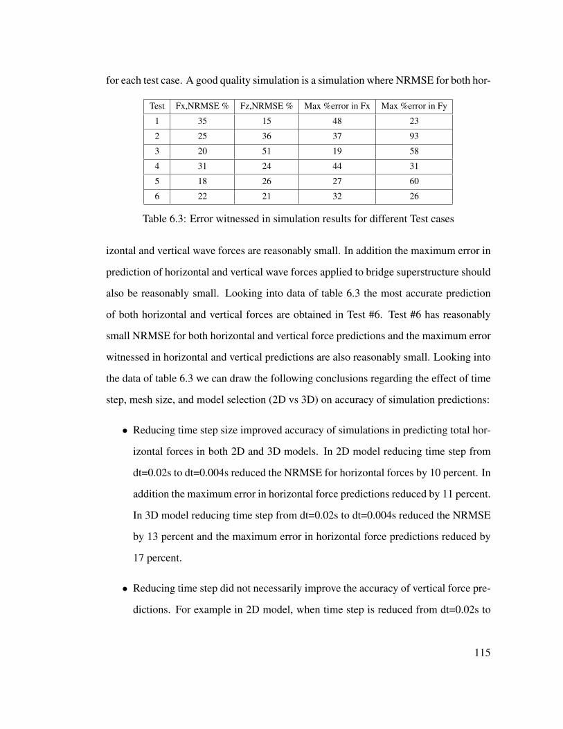
for each test case. A good quality simulation is a simulation where NRMSE for both hor-
Test Fx,NRMSE % Fz,NRMSE % Max %error in Fx Max %error in Fy
1 35 15 48 23
2 25 36 37 93
3 20 51 19 58
4 31 24 44 31
5 18 26 27 60
6 22 21 32 26
Table 6.3: Error witnessed in simulation results for different Test cases
izontal and vertical wave forces are reasonably small. In addition the maximum error in
prediction of horizontal and vertical wave forces applied to bridge superstructure should
also be reasonably small. Looking into data of table 6.3 the most accurate prediction
of both horizontal and vertical forces are obtained in Test #6. Test #6 has reasonably
small NRMSE for both horizontal and vertical force predictions and the maximum error
witnessed in horizontal and vertical predictions are also reasonably small. Looking into
the data of table 6.3 we can draw the following conclusions regarding the effect of time
step, mesh size, and model selection (2D vs 3D) on accuracy of simulation predictions:
• Reducing time step size improved accuracy of simulations in predicting total hor-
izontal forces in both 2D and 3D models. In 2D model reducing time step from
dt=0.02s to dt=0.004s reduced the NRMSE for horizontal forces by 10 percent. In
addition the maximum error in horizontal force predictions reduced by 11 percent.
In 3D model reducing time step from dt=0.02s to dt=0.004s reduced the NRMSE
by 13 percent and the maximum error in horizontal force predictions reduced by
17 percent.
• Reducing time step did not necessarily improve the accuracy of vertical force pre-
dictions. For example in 2D model, when time step is reduced from dt=0.02s to
115

dt=0.004s (Test #1 and Test #2) the NRMSE increased by 21 percent and max-
imum error in vertical force increased by 70 percent. In the same way, in 3D
model when time step reduced from dt=0.02s to dt=0.004s (Test #4 and Test #5)
the NRMSE increased by 2 percent and maximum error in vertical force increased
by 29 percent.
• Reducing time step from dt=0.02s to dt=0.004s improved vertical force predic-
tions only in 3D model with sufficiently fine mesh in transverse direction (y direc-
tion). Comparison of Test #4 to Test #6 shows that when time step is reduced
from dt=0.02s to dt=0.004s, NRMSE for vertical force reduced by 3 percent and
the maximum error in vertical force prediction is reduced by 5 percent.
• Overall while reducing time step in both 2D and 3D models improved the accuracy
of horizontal force predictions, it did not improve the accuracy of vertical force
predictions significantly. The vertical force predictions only improved slightly in
3D model with sufficiently fine mesh in bridge region in all three directions (Test
#6). In all other cases (Test #2 and Test #5) when the time step was reduced, the
error in vertical forces were amplified.
• Comparison of Test #5 to Test #6 shows that when time step size of dt=Tp/625 was
used, refining the mesh in bridge region improved the maximum error in vertical
force prediction by 34 percent. How ever as we see NRMSE and maximum error
in horizontal force increased by 4 percent and 5 percent respectively. This could
be attributed to larger mesh aspect ratio used in Test #5 in free surface region. In
Test #5 the mesh aspect ratio in free surface region was 2.4. In Test #6 the mesh
aspect ratio in free surface region was 4.8.
• In order to accurately model both quasi steady and slamming oscillations, a 3D
model with a time step size of order of dt=0.004s or dt=Tp/625 and a sufficiently
116

small mesh in all three directions in bridge region is required. When time step
size is reduced, failure to properly refine mesh in bridge region would create very
large error for wave heights which contain slamming oscillations (maximum error
in vertical force increased by 29 percent in Test #5 compared to Test #4).
6.5 Guidelines for Choosing Mesh and Time Step Size
in Wave-Structure Interaction Problems
Data of table 6.3) shows that the two phase Navier Stokes equations are very sensitive
to the choice of mesh size and time step for problems in which air entrapment sig-
nificantly influences magnitude of forces applied to structure. Using time step sizes
bigger than dt=Tp/125 causes excessive wave dissipation which will cause the wave to
die out quickly before reaching the bridge and can not model the complex wave-bridge
interaction very accurately. In order to capture slamming oscillations and improve the
accuracy of horizontal force predictions, time step size of order of dt=Tp/625 or smaller
is required. With this time step, the mesh used is also required to be sufficiently fine.
Otherwise reducing the time step will amplify the error in vertical force predictions in
both 2D and 3D models. Error generated in vertical force predictions due to reduction
in time step is mainly due to inaccurate modeling of air movement between cavities that
exist between bridge girders and diaphragms. The best result obtained was for Test #6
in which the following mesh was used in different simulation regions. Directions x, y
and z are shown in figure 5.19.
117
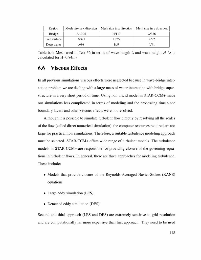
Region Mesh size in x direction Mesh size in z direction Mesh size in y direction
Bridge λ/1305 H/117 λ/326
Free surface λ/391 H/35 λ/82
Deep water λ/98 H/9 λ/41
Table 6.4: Mesh used in Test #6 in terms of wave length λ and wave height H (λ is
calculated for H=0.84m)
6.6 Viscous Effects
In all previous simulations viscous effects were neglected because in wave-bridge inter-
action problem we are dealing with a large mass of water interacting with bridge super-
structure in a very short period of time. Using non viscid model in STAR-CCM+ made
our simulations less complicated in terms of modeling and the processing time since
boundary layers and other viscous effects were not resolved.
Although it is possible to simulate turbulent flow directly by resolving all the scales
of the flow (called direct numerical simulation), the computer resources required are too
large for practical flow simulations. Therefore, a suitable turbulence modeling approach
must be selected. STAR-CCM+ offers wide range of turbulent models. The turbulence
models in STAR-CCM+ are responsible for providing closure of the governing equa-
tions in turbulent flows. In general, there are three approaches for modeling turbulence.
These include:
• Models that provide closure of the Reynolds-Averaged Navier-Stokes (RANS)
equations.
• Large eddy simulation (LES).
• Detached eddy simulation (DES).
Second and third approach (LES and DES) are extremely sensitive to grid resolution
and are computationally far more expensive than first approach. They need to be used
118
for a group of problems in which resolving the small time and length scales are indeed
justified.
STAR-CCM+ offers four major classes of turbulent models based on Reynolds-
Averaged Navier-Stokes (RANS) equations. These include: Spalart-Allmaras, K-
Epsilon , K-Omega and Reynolds stress transport models. CD-adapco (2010) provides
broad guideline to the applicability of each of these models. Further guidance on select-
ing the specific model variants can be found within the sections that provide details
about the models in STAR-CCM+ manual ( CD-adapco (2010)). In this research we
used K-Omega model to evaluate the magnitude of viscous forces in wave-bridge inter-
action problem. K-Omega model is essentially very similar to K-Epsilon in that two
transport equations are solved, but differ in the choice of the second transported turbu-
lence variable ( CD-adapco (2010)). The turbulent equations solved include two vari-
ables, the turbulent kinetic energy K and a quantity called ω which is defined as specific
dissipation rate per unit turbulent energy. One advantage of K-Omega model over K-
Epsilon model is its improved performance for boundary layers under adverse pressure
gradients. However, the most important advantage of K-omega over K-Epsilon model
is that it can be applied throughout the boundary layer, including the viscous-dominated
region, without further modification. Furthermore, the standard K-Omega model can
be used in this mode without requiring the computation of wall distance ( CD-adapco
(2010)). The biggest short coming of the K-Omega model boundary layer computations
is that it is very sensitive to the values of ω in the free stream. This shortcoming was
addressed in STAR-CCM+ by introduction of SST K-Omega Model which improves
original K-Omega model based on the paper by Menter (1994). Menter (1994) essen-
tially blended K-Epsilon model in the far-field with a K-Omega model near the wall.
This approach improves the biggest drawback in applying K-Omega model to practical
flow simulations.
119
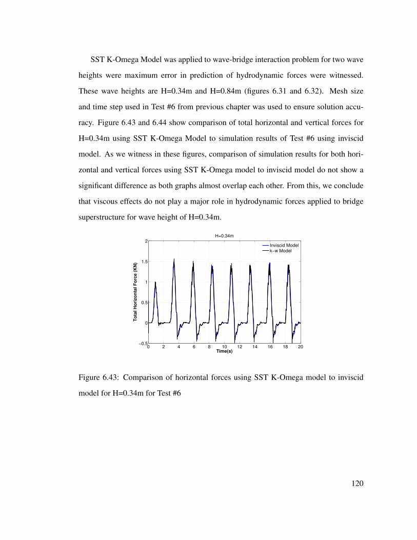
SST K-Omega Model was applied to wave-bridge interaction problem for two wave
heights were maximum error in prediction of hydrodynamic forces were witnessed.
These wave heights are H=0.34m and H=0.84m (figures 6.31 and 6.32). Mesh size
and time step used in Test #6 from previous chapter was used to ensure solution accu-
racy. Figure 6.43 and 6.44 show comparison of total horizontal and vertical forces for
H=0.34m using SST K-Omega Model to simulation results of Test #6 using inviscid
model. As we witness in these figures, comparison of simulation results for both hori-
zontal and vertical forces using SST K-Omega model to inviscid model do not show a
significant difference as both graphs almost overlap each other. From this, we conclude
that viscous effects do not play a major role in hydrodynamic forces applied to bridge
superstructure for wave height of H=0.34m.
0 2 4 6 8 10 12 14 16 18 20−0.5
0
0.5
1
1.5
2
Time(s)
To
tal H
ori
zo
nta
l F
orc
e (
KN
)
H=0.34m
Inviscid Modelk−w Model
Figure 6.43: Comparison of horizontal forces using SST K-Omega model to inviscid
model for H=0.34m for Test #6
120
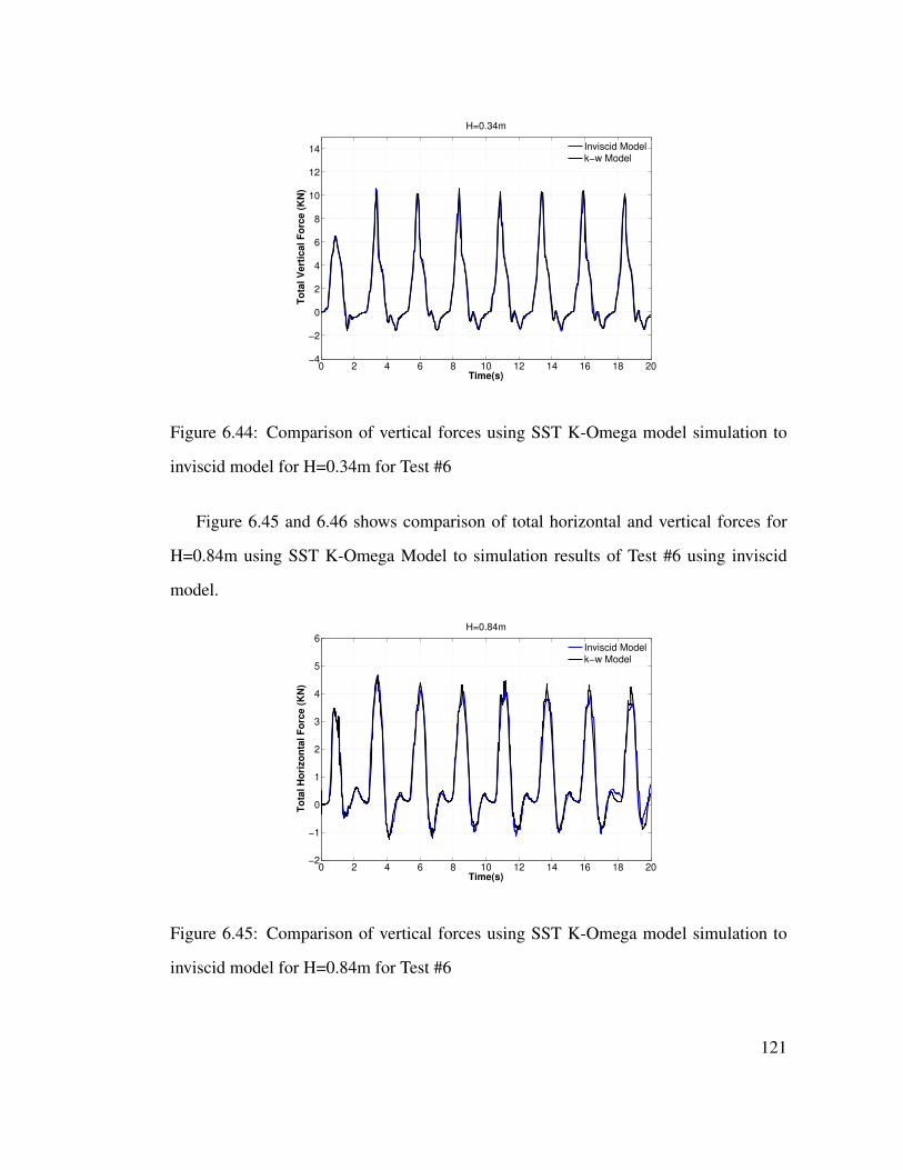
0 2 4 6 8 10 12 14 16 18 20−4
−2
0
2
4
6
8
10
12
14
Time(s)
To
tal V
ert
ical F
orc
e (
KN
)
H=0.34m
Inviscid Modelk−w Model
Figure 6.44: Comparison of vertical forces using SST K-Omega model simulation to
inviscid model for H=0.34m for Test #6
Figure 6.45 and 6.46 shows comparison of total horizontal and vertical forces for
H=0.84m using SST K-Omega Model to simulation results of Test #6 using inviscid
model.
0 2 4 6 8 10 12 14 16 18 20−2
−1
0
1
2
3
4
5
6
Time(s)
To
tal H
ori
zo
nta
l F
orc
e (
KN
)
H=0.84m
Inviscid Modelk−w Model
Figure 6.45: Comparison of vertical forces using SST K-Omega model simulation to
inviscid model for H=0.84m for Test #6
121
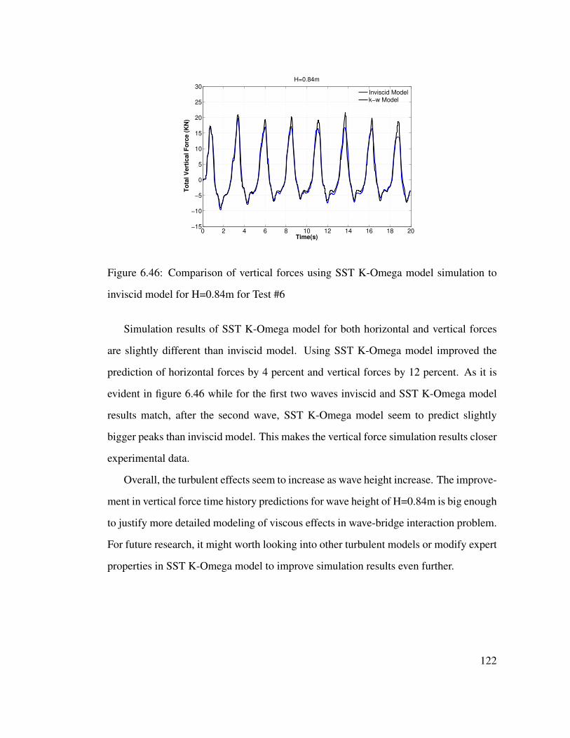
0 2 4 6 8 10 12 14 16 18 20−15
−10
−5
0
5
10
15
20
25
30
Time(s)
To
tal V
ert
ical F
orc
e (
KN
)
H=0.84m
Inviscid Modelk−w Model
Figure 6.46: Comparison of vertical forces using SST K-Omega model simulation to
inviscid model for H=0.84m for Test #6
Simulation results of SST K-Omega model for both horizontal and vertical forces
are slightly different than inviscid model. Using SST K-Omega model improved the
prediction of horizontal forces by 4 percent and vertical forces by 12 percent. As it is
evident in figure 6.46 while for the first two waves inviscid and SST K-Omega model
results match, after the second wave, SST K-Omega model seem to predict slightly
bigger peaks than inviscid model. This makes the vertical force simulation results closer
experimental data.
Overall, the turbulent effects seem to increase as wave height increase. The improve-
ment in vertical force time history predictions for wave height of H=0.84m is big enough
to justify more detailed modeling of viscous effects in wave-bridge interaction problem.
For future research, it might worth looking into other turbulent models or modify expert
properties in SST K-Omega model to improve simulation results even further.
122
Chapter 7
SCALE EFFECTS ON
HYDRODYNAMIC FORCES AND
COMPARISON OF SIMULATED
FORCES TO AASHTO GUIDELINES
7.1 Scale Effects
This chapter deals with transfer of the previous supercomputer models of wave bridge
interaction from laboratory scales to large scales and investigating the effect of scaling
on hydrodynamic forces obtained based on Froude similitude law.
In all hydraulic models, geometric, kinematic, and dynamic similarity is important.
The geometric scaling is handled by maintaining a single length scale between the pro-
totypes and the models. The kinematic and dynamic scaling is handled by maintaining
a single velocity scale ratio between prototypes and models. In hydraulic models, in
general its recommended to meet both Froude and Cauchy similitude criteria ( Hughes
(1993). How ever in reality it is hard to meet both of these criteria at the same time.
Therefore usually Cauchy criteria is neglected. In this problem since the role of com-
pressed air might be significant, disregarding Cauchy criteria might cause dispropor-
tionably high forces due to compression of air.
123

The similarity criteria which is commonly used in wave structure interaction prob-
lems is usually Froude scaling (as apposed to Reynolds number similitude) because
magnitude of inertia forces are significantly bigger than viscous forces. Although
Froude similarity generally plays a more important role in gravity surface water flow,
effects of turbulence may not be negligible when wave interacts with bridge superstruc-
ture.
In this study, numerical simulations were conducted to examine errors in applying
Froude similitude law in modeling wave-bridge interaction. This is done by making
a prototype bridge by scaling the original bridge analyzed in previous section to exact
dimensions of old Escambia Bay Bridge. Based on Froude similitude law the following
relationships exist between model and prototype dimensions, velocities and forces:
Lr =Lp
Lm
(7.1)
Vr ∼√
Lr
tr =Lr
Vr
∼√
Lr
Fr = mrar = ρrL3r
Lr
t2r∼ L3
r
where Lr is length ratio, tr is time ratio, and Fr is force ratio. Applying these formulas to
simulation parameters used in previous chapter we get equivalent parameters that need
to be used for prototype bridge. Table 7.1 shows an example of relationship between
model and prototype simulation parameters for wave height of H=0.34m. Simulation
Parameter Model (1:5) Prototype(1:1)
Wave Height, H 0.34 m 1.7 m
Water depth, d 1.89 m 9.45 m
Wave Period, T 2.5 s 5.59 s
Table 7.1: Example of relationship between model and prototype wave condition
124
domain is meshed using mesh configuration used in Test #6. Mesh used for prototype
bridge simulations scaled to prototype length scales which means mesh used in each
mesh region was five times bigger than what was used in simulation done for model
bridge in Test #6. Hence the total number of mesh cells used in simulation domain and
the number of mesh cells per wave length stayed the same as model bridge. For the time
step size, the same time step of dt=Tp/625 in Test #6 which in prototype scale bridge
simulation is approximately dt=0.01s is used to ensure simulation accuracy. There is
no experimental data available for the prototype model, how ever the accuracy of sim-
ulation could be checked by monitoring residuals and convergence as the simulation
progress. These concepts are explained in detail in chapter 5. Simulations for model
bridge were ran for 15 seconds which include the interaction of 3 waves with prototype
bridge superstructure. Figures 7.1 and 7.2 show the average of horizontal and vertical
forces calculated for 3 waves interacting with prototype bridge superstructure (blue dis-
crete horizontal line) compared to average of horizontal and vertical forces in model
bridge adjusted to prototype scale using Froude similitude law (black discrete horizon-
tal line). As it is evident in these two figures, the average of horizontal and vertical
forces in prototype bridge match the average of horizontal and vertical forces in model
bridge adjusted to prototype scale using Froude similitude law. Even for cases where
slamming forces were present figure 7.2 shows that Froude similitude law works well
for scaling both horizontal and vertical forces. It is also interesting to note that similar
to model bridge, the slamming oscillations in vertical force time histories exist only for
some wave heights not for all. These include wave heights of H=1.7m and H=2.15m
(corresponding to H=0.34m and H=0.43m in model bridge). Also, similar to model
bridge simulations in previous chapter, horizontal force time history does not show any
slamming oscillations.
125
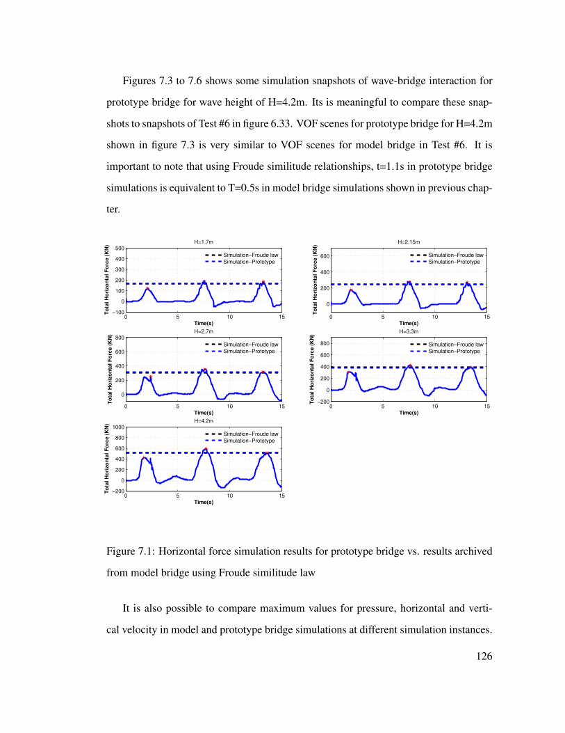
Figures 7.3 to 7.6 shows some simulation snapshots of wave-bridge interaction for
prototype bridge for wave height of H=4.2m. Its is meaningful to compare these snap-
shots to snapshots of Test #6 in figure 6.33. VOF scenes for prototype bridge for H=4.2m
shown in figure 7.3 is very similar to VOF scenes for model bridge in Test #6. It is
important to note that using Froude similitude relationships, t=1.1s in prototype bridge
simulations is equivalent to T=0.5s in model bridge simulations shown in previous chap-
ter.
0 5 10 15−100
0
100
200
300
400
500
Time(s)
To
tal
Ho
rizo
nta
l F
orc
e (
KN
)
H=1.7m
Simulation−Froude law
Simulation−Prototype
0 5 10 15
0
200
400
600
Time(s)
To
tal
Ho
rizo
nta
l F
orc
e (
KN
)
H=2.15m
Simulation−Froude law
Simulation−Prototype
0 5 10 15
0
200
400
600
800
Time(s)
To
tal
Ho
rizo
nta
l F
orc
e (
KN
)
H=2.7m
Simulation−Froude law
Simulation−Prototype
0 5 10 15−200
0
200
400
600
800
Time(s)
To
tal
Ho
rizo
nta
l F
orc
e (
KN
)
H=3.3m
Simulation−Froude law
Simulation−Prototype
0 5 10 15−200
0
200
400
600
800
1000
Time(s)
To
tal
Ho
rizo
nta
l F
orc
e (
KN
)
H=4.2m
Simulation−Froude law
Simulation−Prototype
Figure 7.1: Horizontal force simulation results for prototype bridge vs. results archived
from model bridge using Froude similitude law
It is also possible to compare maximum values for pressure, horizontal and verti-
cal velocity in model and prototype bridge simulations at different simulation instances.
126
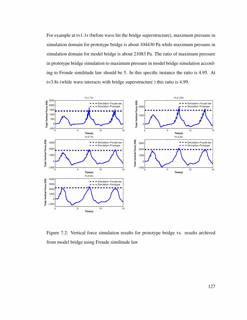
For example at t=1.1s (before wave hit the bridge superstructure), maximum pressure in
simulation domain for prototype bridge is about 104430 Pa while maximum pressure in
simulation domain for model bridge is about 21083 Pa. The ratio of maximum pressure
in prototype bridge simulation to maximum pressure in model bridge simulation accord-
ing to Froude similitude law should be 5. In this specific instance the ratio is 4.95. At
t=3.8s (while wave interacts with bridge superstructure ) this ratio is 4.99.
0 5 10 15−500
0
500
1000
1500
2000
2500
Time(s)
To
tal
Ve
rtic
al
Fo
rce
(K
N)
H=1.7m
Simulation−Froude law
Simulation−Prototype
0 5 10 15
0
1000
2000
Time(s)
To
tal
Ve
rtic
al
Fo
rce
(K
N)
H=2.15m
Simulation−Froude law
Simulation−Prototype
0 5 10 15−1000
0
1000
2000
3000
Time(s)
To
tal
Ve
rtic
al
Fo
rce
(K
N)
H=2.7m
Simulation−Froude law
Simulation−Prototype
0 5 10 15−1000
0
1000
2000
3000
Time(s)
To
tal
Ve
rtic
al
Fo
rce
(K
N)
H=3.3m
Simulation−Froude law
Simulation−Prototype
0 5 10 15
−1000
0
1000
2000
3000
4000
Time(s)
To
tal
Ve
rtic
al
Fo
rce
(K
N)
H=4.2m
Simulation−Froude law
Simulation−Prototype
Figure 7.2: Vertical force simulation results for prototype bridge vs. results archived
from model bridge using Froude similitude law
127
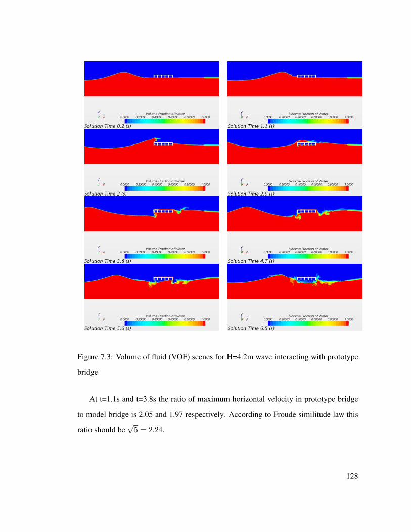
Figure 7.3: Volume of fluid (VOF) scenes for H=4.2m wave interacting with prototype
bridge
At t=1.1s and t=3.8s the ratio of maximum horizontal velocity in prototype bridge
to model bridge is 2.05 and 1.97 respectively. According to Froude similitude law this
ratio should be√5 = 2.24.
128
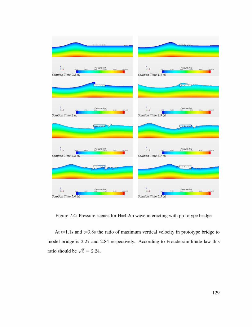
Figure 7.4: Pressure scenes for H=4.2m wave interacting with prototype bridge
At t=1.1s and t=3.8s the ratio of maximum vertical velocity in prototype bridge to
model bridge is 2.27 and 2.84 respectively. According to Froude similitude law this
ratio should be√5 = 2.24.
129
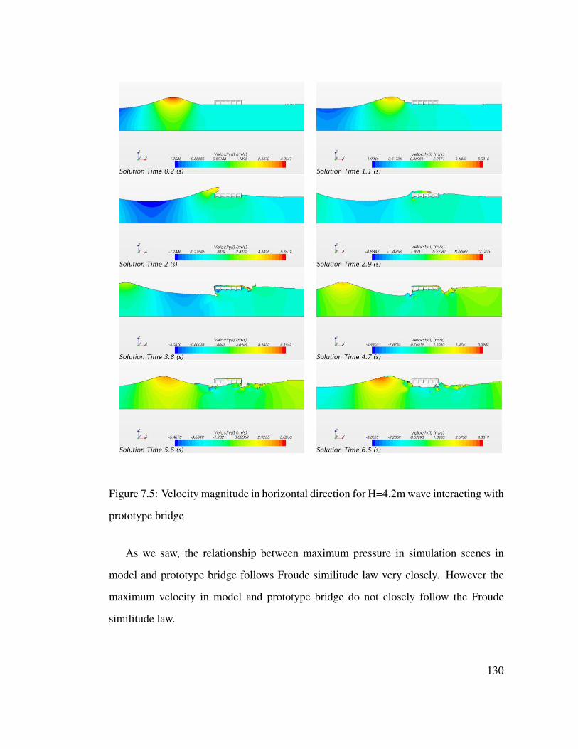
Figure 7.5: Velocity magnitude in horizontal direction for H=4.2m wave interacting with
prototype bridge
As we saw, the relationship between maximum pressure in simulation scenes in
model and prototype bridge follows Froude similitude law very closely. However the
maximum velocity in model and prototype bridge do not closely follow the Froude
similitude law.
130
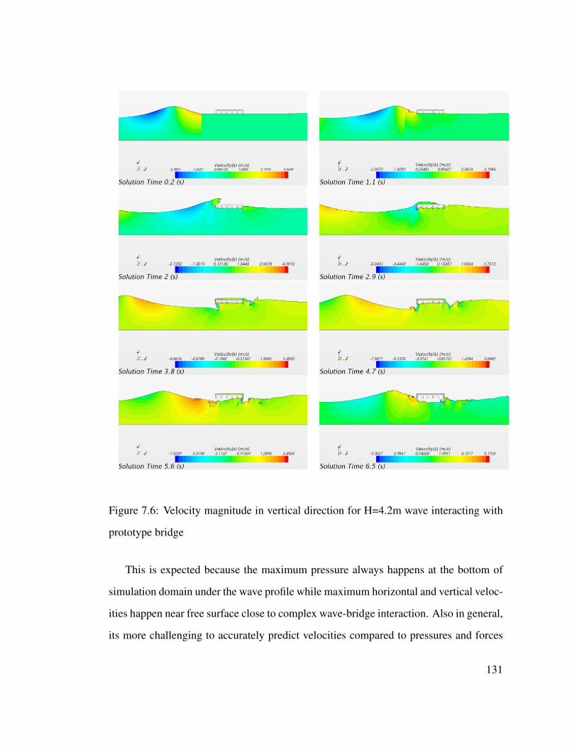
Figure 7.6: Velocity magnitude in vertical direction for H=4.2m wave interacting with
prototype bridge
This is expected because the maximum pressure always happens at the bottom of
simulation domain under the wave profile while maximum horizontal and vertical veloc-
ities happen near free surface close to complex wave-bridge interaction. Also in general,
its more challenging to accurately predict velocities compared to pressures and forces
131
since they are more sensitive to simulation parameters such as mesh size time step and
numerical models. Nevertheless since hydrodynamic forces applied to prototype bridge
matched the ones calculated from model bridge using Froude similitude law, we can
confidently use Froude similitude law to calculate hydrodynamic forces applied to pro-
totype bridge superstructure using the results for model scale bridge superstructure.
7.2 AASHTO Guidelines
Recently developed AASHTO guidelines AASHTO (2008) for wave forces on coastal
bridges are compared to the previously simulated hydrodynamic forces for both model
and prototype bridges. The equations in the guideline require prototype scale inputs, as
a result, the bridge specimen geometry, water depths, and wave conditions are scaled to
prototype dimensions using Froude scaling explained in previous section. These values
are shown in table 7.1 for wave height of H=0.34m (in model scale) and its correspond-
ing prototype values. The dimensions of the prototype bridge are shown in table 5.1.
The maximum quasi-steady horizontal and vertical forces in kip/ft, including the effect
of variable air entrapment according to the guideline is calculated using following equa-
tions:
FH−MAX = F ∗
H−MAXe−3.18+3.76e(−
ωλ)−0.95[ln( ηmax−zc
db+r)]2
(7.2)
FV−MAX = γwWβ(−1.3Hmax
ds+ 1.8)
[1.35 + 0.35 tanh(1.2(Tp)− 8.5)] (7.3)
(b0 + b1x+b2y+ b3x
2 +b4y2
+b5x
y+ b6x
3)(TAF )
These complicated equations come from extensive studies by Sheppard and Marin
(2009) and the laboratory data from 1/8 scale model wave tank tests at the university
132
of Florida and field data from I10 Escambia Bay Bridges damaged during Hurricane
Ivan AASHTO (2008). The parameters used in these equations are explained in full
detail in section 6.1.2.2 of this guideline. Some of the variable used in these equations
are shown in figure 7.7. In the above equations, γw is unit weight of water taken as
0.0064 kip/ft3, W is some function of wave length λ, maximum wave height Hmax,
and distance from storm water level to the bottom of bridge girder Zc. β is some func-
tion of distance from the storm water level to design wave crest ηmax, Zc, and girder
height+bridge thickness db. y is some function of W and λ. x is some function of Hmax
and λ. Variables b0 to b6 are curve fitting coefficients that are only a function of db.
Equation 7.3 accounts for the air entrapment through Trapped Air Factor (TAF).
TAF is used for reduction in the buoyancy component of the vertical quasi-steady force
due to partial or complete venting of the air between bridge girders and diaphragm. The
effect is to alter the buoyancy force, which only has a vertical component, thus the TAF
is only multiplied times the vertical quasi static force AASHTO (2008). The guideline
coefficients for AASHTO type III girders were used and maximum trapped Air Factor
(TAF) is calculated based on a diaphragm height of 4/5 times the girder height. The
resulting forces were then reduced to model scale and plotted with the measured forces
from experimental data . The guideline also has an empirical equation for calculation of
slamming forces.
133
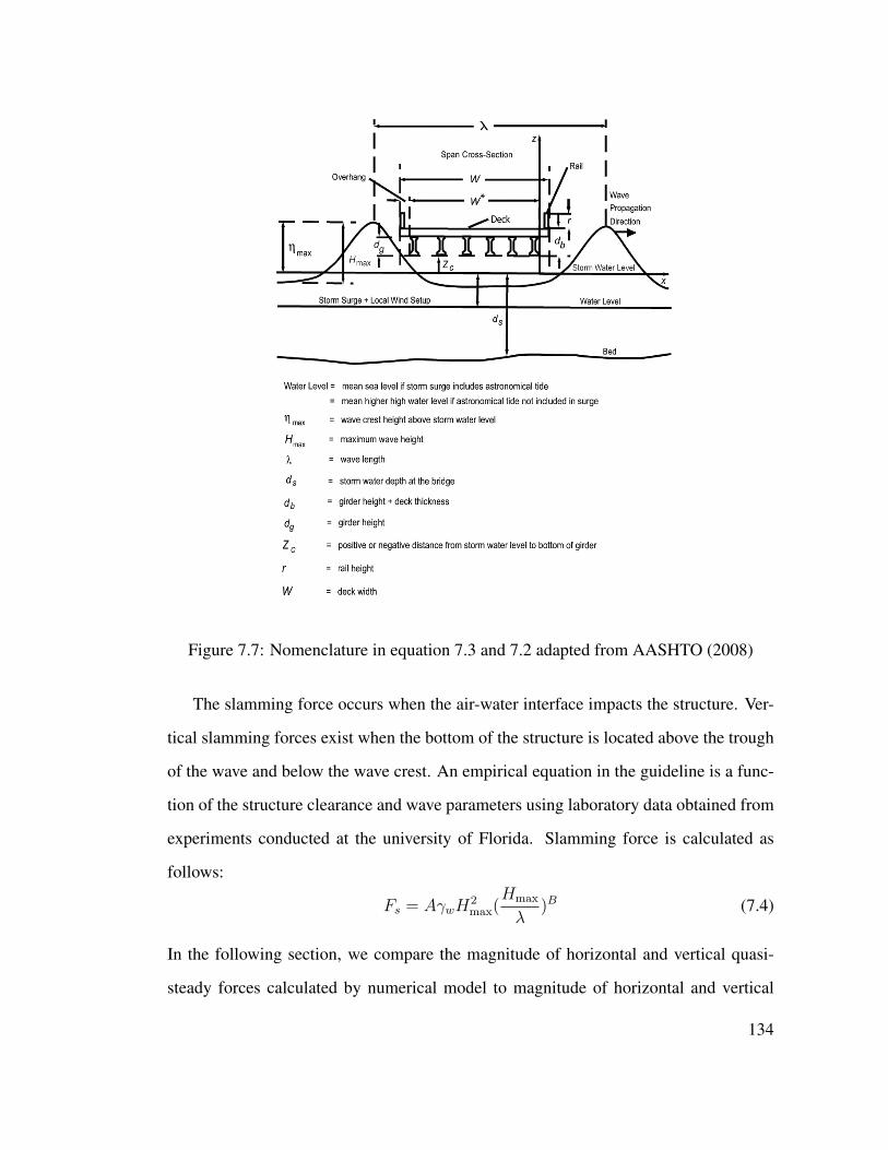
Figure 7.7: Nomenclature in equation 7.3 and 7.2 adapted from AASHTO (2008)
The slamming force occurs when the air-water interface impacts the structure. Ver-
tical slamming forces exist when the bottom of the structure is located above the trough
of the wave and below the wave crest. An empirical equation in the guideline is a func-
tion of the structure clearance and wave parameters using laboratory data obtained from
experiments conducted at the university of Florida. Slamming force is calculated as
follows:
Fs = AγwH2max(
Hmax
λ)B (7.4)
In the following section, we compare the magnitude of horizontal and vertical quasi-
steady forces calculated by numerical model to magnitude of horizontal and vertical
134
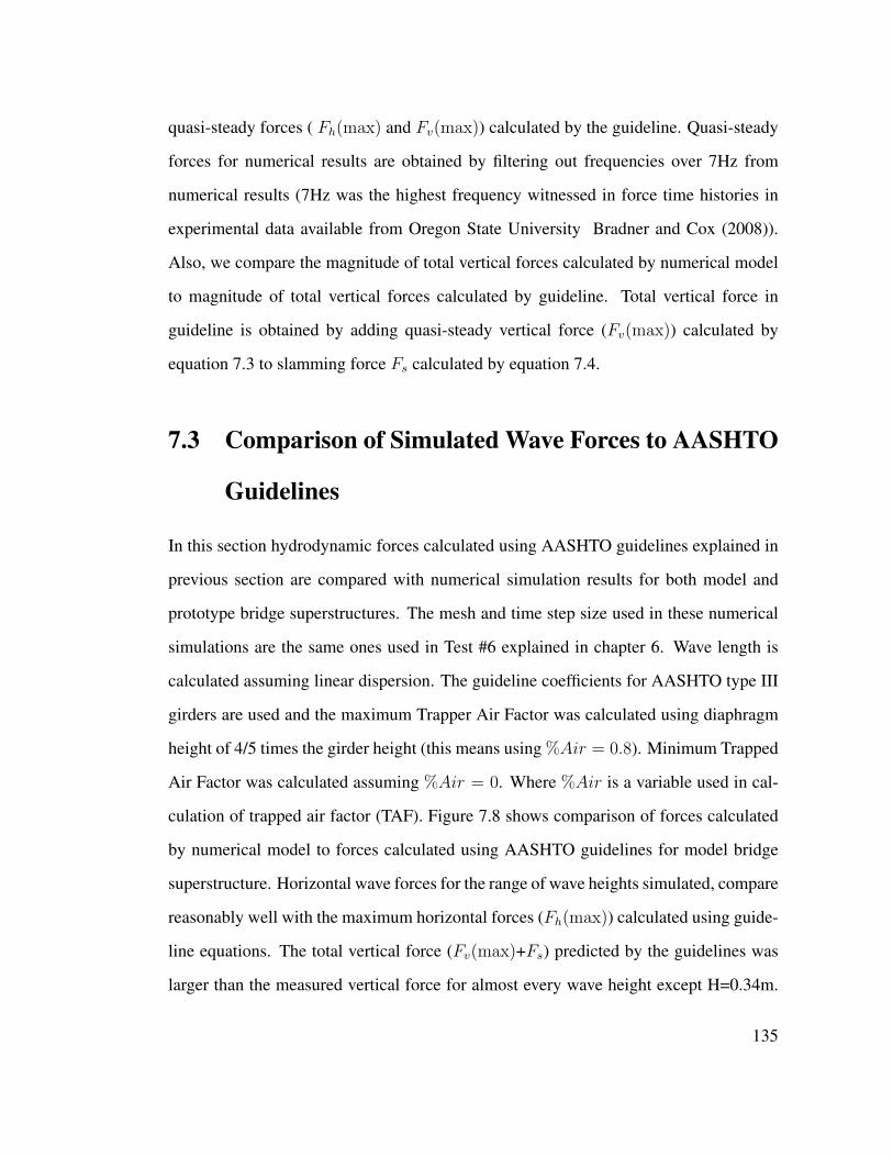
quasi-steady forces ( Fh(max) and Fv(max)) calculated by the guideline. Quasi-steady
forces for numerical results are obtained by filtering out frequencies over 7Hz from
numerical results (7Hz was the highest frequency witnessed in force time histories in
experimental data available from Oregon State University Bradner and Cox (2008)).
Also, we compare the magnitude of total vertical forces calculated by numerical model
to magnitude of total vertical forces calculated by guideline. Total vertical force in
guideline is obtained by adding quasi-steady vertical force (Fv(max)) calculated by
equation 7.3 to slamming force Fs calculated by equation 7.4.
7.3 Comparison of Simulated Wave Forces to AASHTO
Guidelines
In this section hydrodynamic forces calculated using AASHTO guidelines explained in
previous section are compared with numerical simulation results for both model and
prototype bridge superstructures. The mesh and time step size used in these numerical
simulations are the same ones used in Test #6 explained in chapter 6. Wave length is
calculated assuming linear dispersion. The guideline coefficients for AASHTO type III
girders are used and the maximum Trapper Air Factor was calculated using diaphragm
height of 4/5 times the girder height (this means using %Air = 0.8). Minimum Trapped
Air Factor was calculated assuming %Air = 0. Where %Air is a variable used in cal-
culation of trapped air factor (TAF). Figure 7.8 shows comparison of forces calculated
by numerical model to forces calculated using AASHTO guidelines for model bridge
superstructure. Horizontal wave forces for the range of wave heights simulated, compare
reasonably well with the maximum horizontal forces (Fh(max)) calculated using guide-
line equations. The total vertical force (Fv(max)+Fs) predicted by the guidelines was
larger than the measured vertical force for almost every wave height except H=0.34m.
135
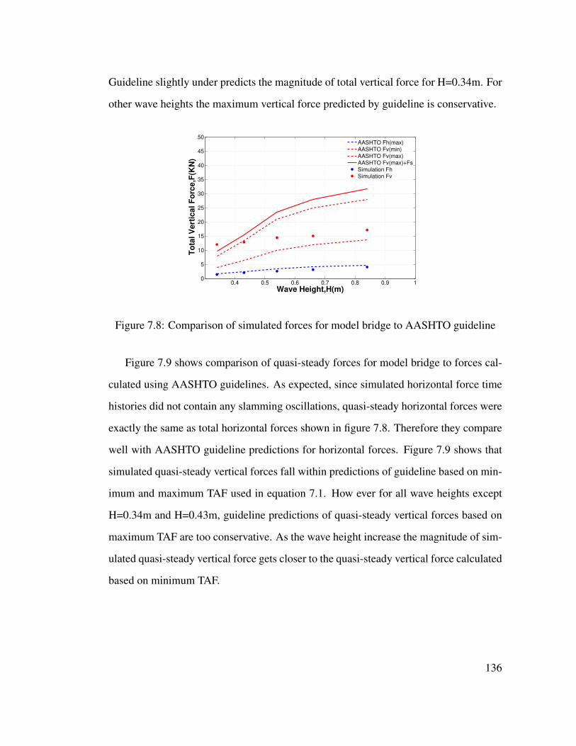
Guideline slightly under predicts the magnitude of total vertical force for H=0.34m. For
other wave heights the maximum vertical force predicted by guideline is conservative.
0.4 0.5 0.6 0.7 0.8 0.9 10
5
10
15
20
25
30
35
40
45
50
Wave Height,H(m)
To
tal
Ve
rtic
al
Fo
rce
,F(K
N)
AASHTO Fh(max)AASHTO Fv(min)AASHTO Fv(max)AASHTO Fv(max)+FsSimulation FhSimulation Fv
Figure 7.8: Comparison of simulated forces for model bridge to AASHTO guideline
Figure 7.9 shows comparison of quasi-steady forces for model bridge to forces cal-
culated using AASHTO guidelines. As expected, since simulated horizontal force time
histories did not contain any slamming oscillations, quasi-steady horizontal forces were
exactly the same as total horizontal forces shown in figure 7.8. Therefore they compare
well with AASHTO guideline predictions for horizontal forces. Figure 7.9 shows that
simulated quasi-steady vertical forces fall within predictions of guideline based on min-
imum and maximum TAF used in equation 7.1. How ever for all wave heights except
H=0.34m and H=0.43m, guideline predictions of quasi-steady vertical forces based on
maximum TAF are too conservative. As the wave height increase the magnitude of sim-
ulated quasi-steady vertical force gets closer to the quasi-steady vertical force calculated
based on minimum TAF.
136
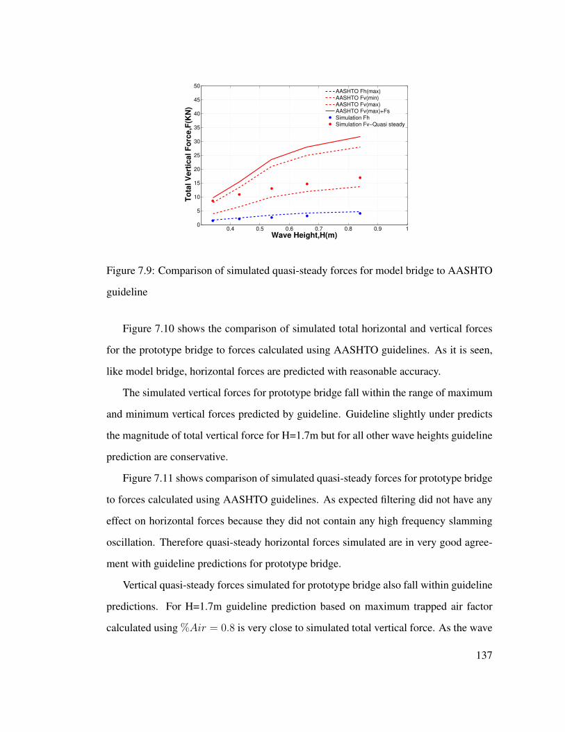
0.4 0.5 0.6 0.7 0.8 0.9 10
5
10
15
20
25
30
35
40
45
50
Wave Height,H(m)
To
tal
Ve
rtic
al
Fo
rce
,F(K
N)
AASHTO Fh(max)AASHTO Fv(min)AASHTO Fv(max)AASHTO Fv(max)+FsSimulation FhSimulation Fv−Quasi steady
Figure 7.9: Comparison of simulated quasi-steady forces for model bridge to AASHTO
guideline
Figure 7.10 shows the comparison of simulated total horizontal and vertical forces
for the prototype bridge to forces calculated using AASHTO guidelines. As it is seen,
like model bridge, horizontal forces are predicted with reasonable accuracy.
The simulated vertical forces for prototype bridge fall within the range of maximum
and minimum vertical forces predicted by guideline. Guideline slightly under predicts
the magnitude of total vertical force for H=1.7m but for all other wave heights guideline
prediction are conservative.
Figure 7.11 shows comparison of simulated quasi-steady forces for prototype bridge
to forces calculated using AASHTO guidelines. As expected filtering did not have any
effect on horizontal forces because they did not contain any high frequency slamming
oscillation. Therefore quasi-steady horizontal forces simulated are in very good agree-
ment with guideline predictions for prototype bridge.
Vertical quasi-steady forces simulated for prototype bridge also fall within guideline
predictions. For H=1.7m guideline prediction based on maximum trapped air factor
calculated using %Air = 0.8 is very close to simulated total vertical force. As the wave
137
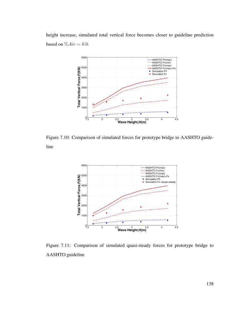
height increase, simulated total vertical force becomes closer to guideline prediction
based on %Air = 0.0.
1.5 2 2.5 3 3.5 4 4.50
1000
2000
3000
4000
5000
6000
Wave Height,H(m)
To
tal
Ve
rtic
al
Fo
rce
,F(K
N)
AASHTO Fh(max)AASHTO Fv(min)AASHTO Fv(max)AASHTO Fv(max)+FsSimulation FhSimulation Fv
Figure 7.10: Comparison of simulated forces for prototype bridge to AASHTO guide-
line
1.5 2 2.5 3 3.5 4 4.50
1000
2000
3000
4000
5000
6000
Wave Height,H(m)
To
tal
Ve
rtic
al
Fo
rce
,F(K
N)
AASHTO Fh(max)AASHTO Fv(min)AASHTO Fv(max)AASHTO Fv(max)+FsSimulation FhSimulation Fv−Quasi steady
Figure 7.11: Comparison of simulated quasi-steady forces for prototype bridge to
AASHTO guideline
138
To sum up, AASHTO guideline was well capable of predicting total horizontal
forces applied to bridge superstructure for both model and prototype bridges. Mag-
nitude of vertical forces calculated using guideline equations are shown to be very sen-
sitive to the value chosen for trapped air factor (TAF) in equation 7.3. Simulated forces
for both model and prototype bridge fell within guideline predictions for the range of
wave heights simulated based on maximum and minimum trapped air factor. Except for
forces calculated for wave height of H=0.34m (H=1.7m in prototype bridge simulations)
inclusion of slamming force Fs in total vertical force was shown to be too conservative.
In addition since slamming force was not present in any experimental data available
from Oregon State University, designers should use their judgment and consider struc-
tural respond when deciding whether or not to include the slamming force in the design
load, as the quasi-steady force alone may be sufficient for most applications.
‘
139

Chapter 8
RETROFITTING OPTIONS
AVAILABLE FOR COASTAL
BRIDGES EXPOSED TO WAVES
To avoid loss of coastal bridges from Hurricane surge wave forces if possible the best
way is to elevate them sufficiently to allow the surge/surface wave to pass under the
bridge superstructure. However, if this is too costly and/or the bridge is already in
existence, it appears that it should be very feasible to connect the bridge components in a
manner, or to take retrofit action, to avoid having the hurricane surge/surface wave dump
the superstructure into the water. One effective way proposed was to improve venting of
underneath regions of bridge superstructure to reduce buoyant forces. This can be done
by selective deck coring and the creation of large holes in span end diaphragms to allow
exchange of trapped air between spans.
In this section two retrofitting options are investigated. These two options are rec-
ommended by AASHTO guidelines and several other reports including Sawyer (2008).
These options are:
• Airvents in bridge deck
• Airvents in bridge diaphragm
The results of using above retrofitting options to wave bridge interaction problem is
presented in the following sections.
140
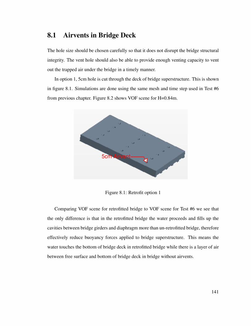
8.1 Airvents in Bridge Deck
The hole size should be chosen carefully so that it does not disrupt the bridge structural
integrity. The vent hole should also be able to provide enough venting capacity to vent
out the trapped air under the bridge in a timely manner.
In option 1, 5cm hole is cut through the deck of bridge superstructure. This is shown
in figure 8.1. Simulations are done using the same mesh and time step used in Test #6
from previous chapter. Figure 8.2 shows VOF scene for H=0.84m.
5cm Airvent
Figure 8.1: Retrofit option 1
Comparing VOF scene for retrofitted bridge to VOF scene for Test #6 we see that
the only difference is that in the retrofitted bridge the water proceeds and fills up the
cavities between bridge girders and diaphragm more than un-retrofitted bridge, therefore
effectively reduce buoyancy forces applied to bridge superstructure. This means the
water touches the bottom of bridge deck in retrofitted bridge while there is a layer of air
between free surface and bottom of bridge deck in bridge without airvents.
141
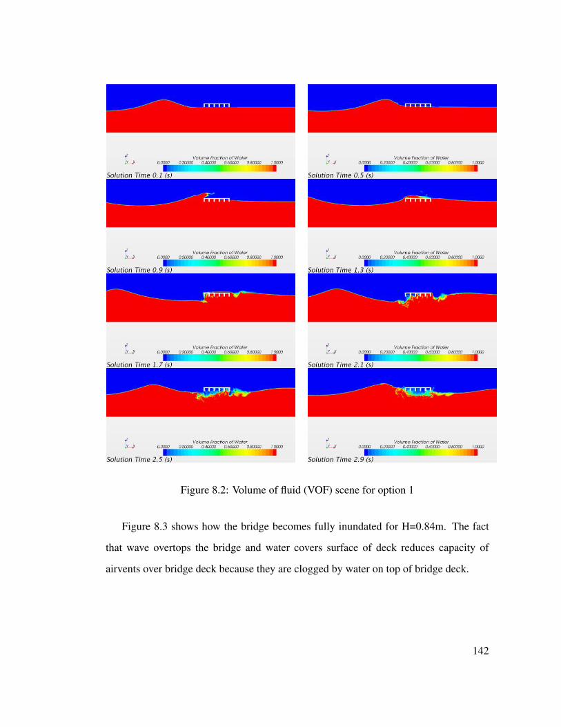
Figure 8.2: Volume of fluid (VOF) scene for option 1
Figure 8.3 shows how the bridge becomes fully inundated for H=0.84m. The fact
that wave overtops the bridge and water covers surface of deck reduces capacity of
airvents over bridge deck because they are clogged by water on top of bridge deck.
142
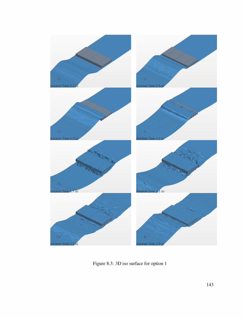
Figure 8.3: 3D iso surface for option 1
143

Comparison of simulations before and after adding the vent hole to bridge deck
(option 1), shows that airvents can be very effective in reducing vertical hydrodynamic
forces for some wave heights. As it is seen in figure 8.6 airvents in bridge deck have
a two fold effect on total vertical hydrodynamic forces: they reduce the magnitude of
slamming oscillation and they decrease the overall quasi-steady vertical force. Usage
of 5cm air vent in bridge deck causes about 60 percent reduction in total vertical wave
forces for H=0.34m. How ever as wave height increase the efficacy of airvents in reduc-
ing hydrodynamic forces decrease. For example, for H=0.84m airvents reduce total ver-
tical force by only 17 percent (figure 8.7). This may be because of one of the following
reasons or combination of both:
• As wave height increase water particle velocities also increase. This means cav-
ities under the bridge are filled much faster and there may be not enough time
for 5cm airvent to fully vent out the air between bridge girders and diaphragms.
This means some air will remain between bridge girders and diaphragm therefore
the vertical forces do not decrease for bigger waves as much as they decrease for
smaller waves.
• Another reason for airvents not being effective for bigger waves could be the water
overtopping the bridge deck. Water covering the surface of bridge deck may clog
the vents and prevent the air from venting out of deck air vents.
Option 1 retrofit also influence total horizontal forces applied to bridge superstructure.
While for H=0.34m airvents reduce total horizontal forces by 15 percent (figure 8.4) ,
They seem to slightly increase horizontal forces for other wave heights. For example,
for H=0.84m (figure 8.5) total horizontal forces increase by 7 percent.
144
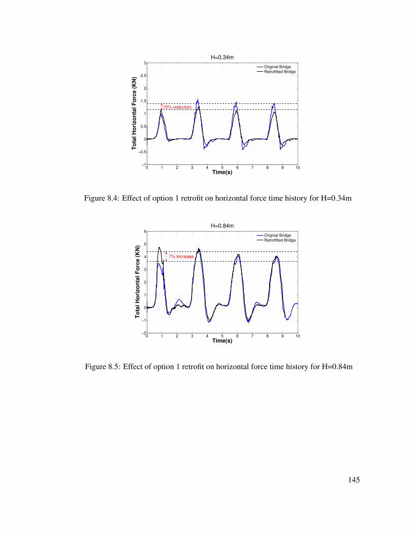
0 1 2 3 4 5 6 7 8 9 10−1
−0.5
0
0.5
1
1.5
2
2.5
3
Time(s)
To
tal
Ho
rizo
nta
l F
orc
e (
KN
)
H=0.34m
Original Bridge
Retrofitted Bridge
15% reduction
Figure 8.4: Effect of option 1 retrofit on horizontal force time history for H=0.34m
0 1 2 3 4 5 6 7 8 9 10−2
−1
0
1
2
3
4
5
6
Time(s)
To
tal
Ho
rizo
nta
l F
orc
e (
KN
)
H=0.84m
Original Bridge
Retrofitted Bridge
7% increase
Figure 8.5: Effect of option 1 retrofit on horizontal force time history for H=0.84m
145
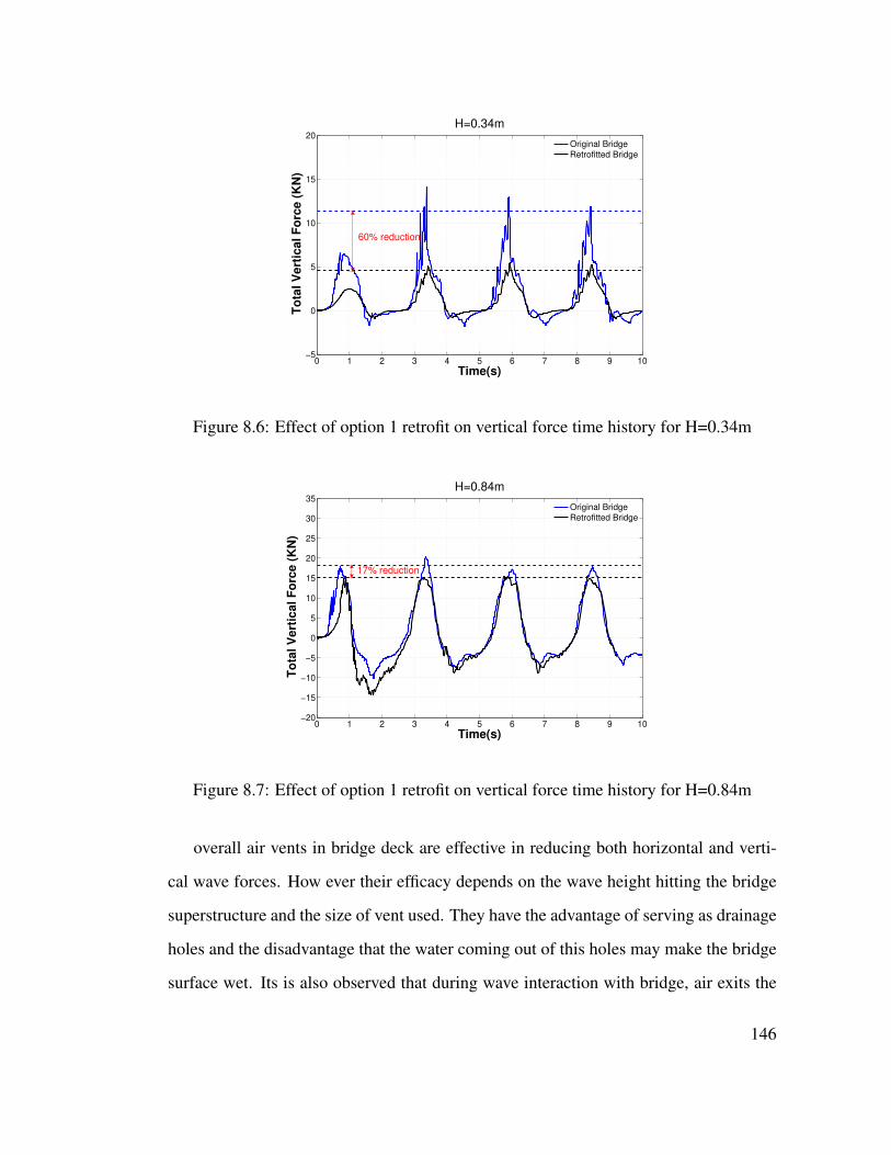
0 1 2 3 4 5 6 7 8 9 10−5
0
5
10
15
20
Time(s)
To
tal
Ve
rtic
al
Fo
rce
(K
N)
H=0.34m
Original Bridge
Retrofitted Bridge
60% reduction
Figure 8.6: Effect of option 1 retrofit on vertical force time history for H=0.34m
0 1 2 3 4 5 6 7 8 9 10−20
−15
−10
−5
0
5
10
15
20
25
30
35
Time(s)
To
tal
Ve
rtic
al
Fo
rce
(K
N)
H=0.84m
Original Bridge
Retrofitted Bridge
17% reduction
Figure 8.7: Effect of option 1 retrofit on vertical force time history for H=0.84m
overall air vents in bridge deck are effective in reducing both horizontal and verti-
cal wave forces. How ever their efficacy depends on the wave height hitting the bridge
superstructure and the size of vent used. They have the advantage of serving as drainage
holes and the disadvantage that the water coming out of this holes may make the bridge
surface wet. Its is also observed that during wave interaction with bridge, air exits the
146

holes with a very high velocity reaching about 40 m/s (for H=0.84m). This is something
that needs to be considered as it might cause problems for traffic passing over the bridge
superstructure. The effect of air vents on horizontal and vertical forces for different wave
height for option 1 retrofit is shown in figure 8.8 and 8.9. As it is evident in these figures
the option 1 retrofit reduces vertical forces up to 62 percent for H=0.34m. As the wave
height increase, the efficacy of air vents decrease reaching 17 percent for H=0.84m.
Retrofit option 1 also influences horizontal hydrodynamic forces. For H=0.34m air
vents reduce horizontal force by 18 percent whereas for other wave heights the hor-
izontal forces slightly increase. For example for H=0.84m, retrofit option 1 increase
total horizontal force by 9 percent. The increase in horizontal force in retrofitted bridge
is likely due to increase in areas of bridge superstructure that is exposed to horizontal
wave momentum as a result of water penetrating the cavities between bridge girders and
diaphragms.
-100.00
-80.00
-60.00
-40.00
-20.00
0.00
20.00
40.00
60.00
80.00
100.00
0.34 0.43 0.54 0.66 0.84
Eff
ect
of
air
ve
nt
on
ho
rizo
nta
l fo
rce
Wave Height H (m)
Figure 8.8: Effect of option 1 retrofit on horizontal force for various wave heights
147
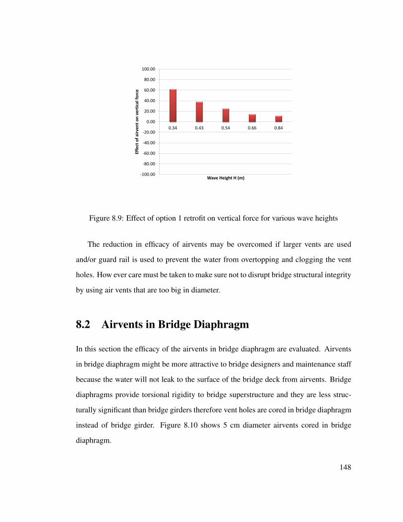
-100.00
-80.00
-60.00
-40.00
-20.00
0.00
20.00
40.00
60.00
80.00
100.00
0.34 0.43 0.54 0.66 0.84
Eff
ect
of
air
ve
nt
on
ve
rtic
al
forc
e
Wave Height H (m)
Figure 8.9: Effect of option 1 retrofit on vertical force for various wave heights
The reduction in efficacy of airvents may be overcomed if larger vents are used
and/or guard rail is used to prevent the water from overtopping and clogging the vent
holes. How ever care must be taken to make sure not to disrupt bridge structural integrity
by using air vents that are too big in diameter.
8.2 Airvents in Bridge Diaphragm
In this section the efficacy of the airvents in bridge diaphragm are evaluated. Airvents
in bridge diaphragm might be more attractive to bridge designers and maintenance staff
because the water will not leak to the surface of the bridge deck from airvents. Bridge
diaphragms provide torsional rigidity to bridge superstructure and they are less struc-
turally significant than bridge girders therefore vent holes are cored in bridge diaphragm
instead of bridge girder. Figure 8.10 shows 5 cm diameter airvents cored in bridge
diaphragm.
148
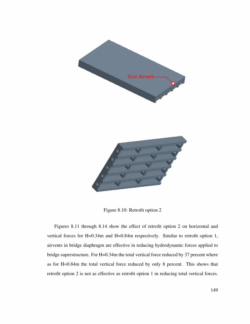
5cm Airvent
Figure 8.10: Retrofit option 2
Figures 8.11 through 8.14 show the effect of retrofit option 2 on horizontal and
vertical forces for H=0.34m and H=0.84m respectively. Similar to retrofit option 1,
airvents in bridge diaphragm are effective in reducing hydrodynamic forces applied to
bridge superstructure. For H=0.34m the total vertical force reduced by 37 percent where
as for H=0.84m the total vertical force reduced by only 8 percent. This shows that
retrofit option 2 is not as effective as retrofit option 1 in reducing total vertical forces.
149
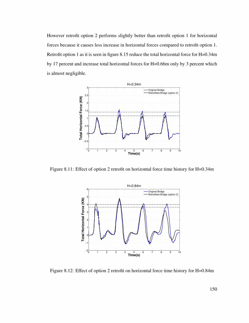
However retrofit option 2 performs slightly better than retrofit option 1 for horizontal
forces because it causes less increase in horizontal forces compared to retrofit option 1.
Retrofit option 1 as it is seen in figure 8.15 reduce the total horizontal force for H=0.34m
by 17 percent and increase total horizontal forces for H=0.66m only by 3 percent which
is almost negligible.
0 1 2 3 4 5 6 7 8 9 10−1
−0.5
0
0.5
1
1.5
2
2.5
3
Time(s)
To
tal
Ho
rizo
nta
l F
orc
e (
KN
)H=0.34m
Original Bridge
Retrofitted Bridge (option 2)
Figure 8.11: Effect of option 2 retrofit on horizontal force time history for H=0.34m
0 1 2 3 4 5 6 7 8 9 10−2
−1
0
1
2
3
4
5
6
Time(s)
To
tal
Ho
rizo
nta
l F
orc
e (
KN
)
H=0.84m
Original Bridge
Retrofitted Bridge (option 2)
Figure 8.12: Effect of option 2 retrofit on horizontal force time history for H=0.84m
150
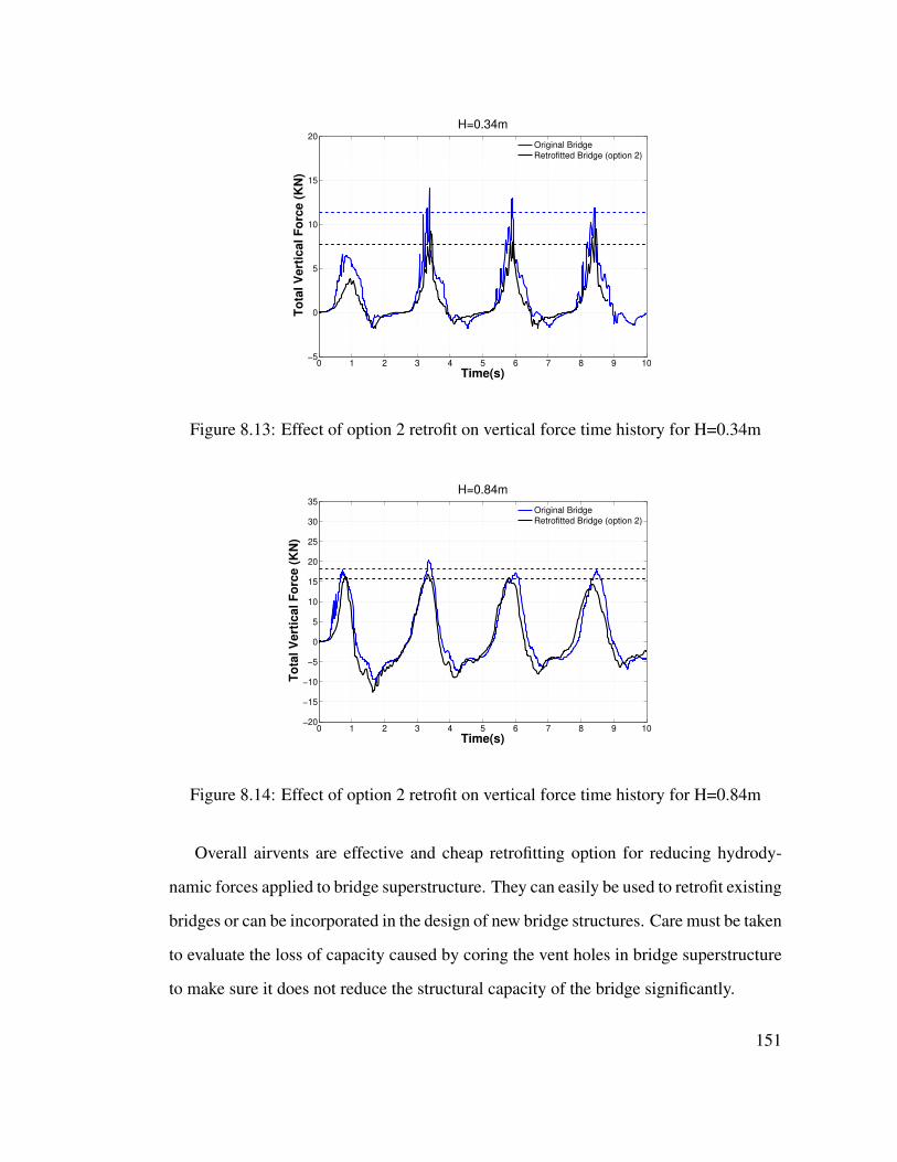
0 1 2 3 4 5 6 7 8 9 10−5
0
5
10
15
20
Time(s)
To
tal
Ve
rtic
al
Fo
rce
(K
N)
H=0.34m
Original Bridge
Retrofitted Bridge (option 2)
Figure 8.13: Effect of option 2 retrofit on vertical force time history for H=0.34m
0 1 2 3 4 5 6 7 8 9 10−20
−15
−10
−5
0
5
10
15
20
25
30
35
Time(s)
To
tal
Ve
rtic
al
Fo
rce
(K
N)
H=0.84m
Original Bridge
Retrofitted Bridge (option 2)
Figure 8.14: Effect of option 2 retrofit on vertical force time history for H=0.84m
Overall airvents are effective and cheap retrofitting option for reducing hydrody-
namic forces applied to bridge superstructure. They can easily be used to retrofit existing
bridges or can be incorporated in the design of new bridge structures. Care must be taken
to evaluate the loss of capacity caused by coring the vent holes in bridge superstructure
to make sure it does not reduce the structural capacity of the bridge significantly.
151
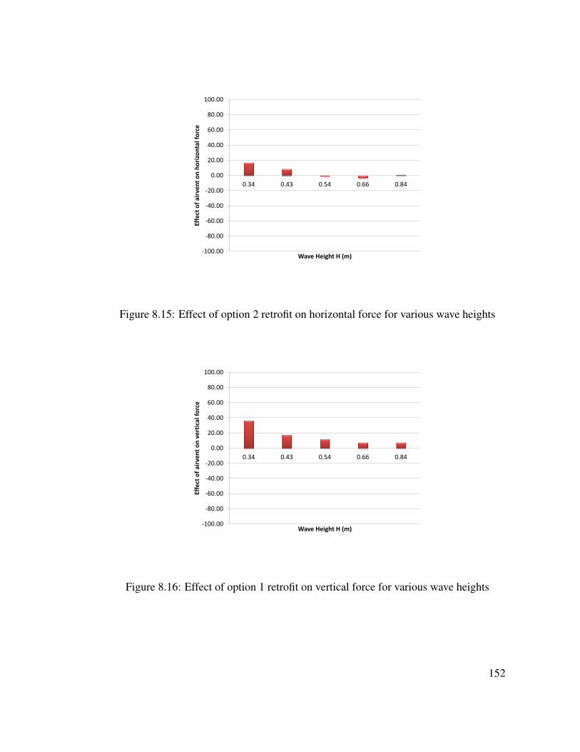
-100.00
-80.00
-60.00
-40.00
-20.00
0.00
20.00
40.00
60.00
80.00
100.00
0.34 0.43 0.54 0.66 0.84
Eff
ect
of
air
ve
nt
on
ho
rizo
nta
l fo
rce
Wave Height H (m)
Figure 8.15: Effect of option 2 retrofit on horizontal force for various wave heights
-100.00
-80.00
-60.00
-40.00
-20.00
0.00
20.00
40.00
60.00
80.00
100.00
0.34 0.43 0.54 0.66 0.84
Eff
ect
of
air
ve
nt
on
ve
rtic
al
forc
e
Wave Height H (m)
Figure 8.16: Effect of option 1 retrofit on vertical force for various wave heights
152
Chapter 9
CONCLUDING REMARKS
Understanding the forces acting on highway bridge superstructure is critical to improve
the durability of bridges, which can, even if infrequently, be overtopped in Hurricane
or Tsunami events. The overall objective of the study was to establish validated com-
putational practice to address research needs of the transportation community in bridge
hydraulics via computational fluid dynamic simulations. The study provides modeling
capability for the simulation of waves interacting with a typical highway bridge super-
structure. The followings conclude the findings and achievements of this study:
• In chapter 4 CFD software was validated by modeling a solitary wave interacting
with a simple flat plate. It was shown that the CFD software was well capable of
predicting pressure under the flat plate and velocities at different points inside the
simulation domain. In addition results of simulation was compared with two other
Finite Element codes previously developed. CFD software was able to predict
pressure fluctuations under the flat plate with a better accuracy than two previous
Finite Element codes developed.
• The validated CFD software was applied to 1:5 scaled old Escambia Bay bridge
which was heavily damaged during Hurricane Ivan. Simulation results were com-
pared to experimental data available from the O.H. Hinsdale Wave Research Lab-
oratory at Oregon State University. Six 2D and 3D test cases were designed to
investigate the effect of model selection (2D vs 3D), time step and grid resolution
on simulation accuracy. Simulations were carried out to predict total horizontal
and vertical forces applied to bridge superstructure. It was shown that the two
153
phase Navier stokes equations were very sensitive to mesh size, time step and
boundary conditions used in the simulation. The 2D model was not capable of
predicting horizontal and vertical wave forces with reasonable accuracy in a single
simulation. While the 2D model with the time step size of dt = Tp/125 was capa-
ble of predicting vertical wave forces with reasonable accuracy, it could not pre-
dict horizontal wave forces with good accuracy even when a very fine mesh was
used. Prediction of horizontal wave forces with a reasonable accuracy required
time step size of the order of dt = Tp/625. Reducing time step to Tp/625 in
2D model improved accuracy of horizontal force predictions however it created
excessive oscillatory behavior in vertical force time history which was the result
of inaccurate modeling of air phase movement under bridge superstructure since
the 2D model did not allow the air to move in transverse direction. Test #3 results
showed that horizontal wave forces were not sensitive to air entrapment and exclu-
sion of air phase by letting it vent out of simulation domain in fact improved the
accuracy of horizontal force predictions even with time step size of dt = Tp/125.
3D model predicted horizontal wave forces slightly better than 2D model when
similar time steps were used. 3D model was very sensitive to the mesh size used
in all three dimensions including transverse direction along the bridge girder and
perpendicular to bridge diaphragm. Comparison of Test #5 to Test #6 shows that
refinement of mesh size in transverse direction reduced maximum error in verti-
cal forces by 34 percent (table 6.3). In addition to mesh size, mesh aspect ratio
was also shown to be important. Comparison of Test #5 to Test #6 results showed
the importance of keeping mesh aspect ratio as small as what computer resources
allow. In Test #5 the mesh used in free surface region had aspect ratio of 2.4 while
in Test #6 the mesh used in free surface had aspect ratio of 4.8. This increase in
aspect ratio increased the maximum error in horizontal forces by 5 percent. At the
154
end of chapter 6 meshing guidelines were proposed which were found suitable for
wave-bridge interaction problem with emphasis on accurate modeling of air phase
under the bridge superstructure.
• Some Test #6 force time histories showed oscillatory behavior. This include force
time histories for wave heights of H=0.34m, H=0.43m, and H=0.54m (figure
6.41). As the wave height increased the oscillatory behavior decreased in all test
cases. While biggest amplitude oscillations happened in force time history for
wave height of H=0.34m, force time history for wave height of H=0.84m did not
show any oscillatory behavior. The amplitude of these slamming oscillations in
force time history for wave height of H=0.34m was directly related to mesh size,
time step, and specially to the boundary condition used on the side of simula-
tion domain (2D model vs. 3D model). These high frequency slamming oscilla-
tions were not seen in experimental data available from Oregon State University.
How ever they were witnessed in experimental data available from University
of Florida experiments. This suggests, that existence of slamming oscillations
in force time history depended on experimental setup and bridge superstructure
properties (mass and damping coefficient) under experiment. Since the bridge
superstructure under experiment in Oregon State University was bigger and heav-
ier than bridge superstructure under experiment in University of Florida, we con-
clude that as bridge superstructure gets bigger and heavier the structure does not
respond to a high frequency slamming force. This means as the wave strikes the
bridge, an impact pressure may be generated but this pressure does not show itself
as a reaction force at the bent cap. The large mass of bridge superstructure dissi-
pates this impact. There may cause localized forces and resulting damage such as
concrete spalling or cracking, but it is unlikely that these forces were responsible
for the failures witnessed during Hurricanes Ivan and Katrina. Therefore inclusion
155
of these slamming oscillations witnessed in CFD simulations may not be required
for prototype scale bridge superstructure.
• At the end of chapter 6, effect of turbulent modeling on hydrodynamic forces
applied to bridge superstructure was evaluated by using K-omega turbulent model
and comparing the simulation results to horizontal and vertical forces calculated
using inviscid model. K-omega model, used with default settings in CFD software
and mesh size and time step similar to mesh size and time step used in Test #6,
was not able to decrease the magnitude of error witnessed in force time history
of horizontal and vertical forces for wave height of H=0.34m. For wave height
of H=0.84m, K-omega model was able to improve predictions of horizontal and
vertical forces by 4 percent and 12 percent respectively. This suggests that as
wave height increase and wave-bridge interaction becomes more violent, turbulent
modeling and viscous effects need to be considered.
• Since there are a lot of concerns about scale effects when using empirical equa-
tions which are developed from small scale model experiments especially when
entrapment of air is involved, in chapter 7 CFD software was used to evaluate
scale effects in wave bridge interaction problem. A bridge prototype with old
Escambia Bay bridge dimensions was built. Equivalent wave heights and period
were calculated using Froude similitude laws from the wave heights and periods
used in model simulations. The number of mesh per wave length and time step
used in these simulations were similar to the ones used in Test #6. The forces
obtained from CFD simulations for prototype bridge were compared to forces
calculated using Froude similitude law from model bridge simulations. Both hor-
izontal and vertical forces calculated for the prototype bridge using Froude simil-
itude law matched the simulation results for prototype bridge. In addition force
156
time history for prototype bridge showed a very similar pattern to force time his-
tory for model bridge with slamming oscillation existing for only certain wave
heights (H=1.7m, H=2.15m, H=2.7m). This proves validity of Froude similitude
law for complex wave structure interaction problems even when the effect of air
entrapment and entrainment is considered. In addition, CFD simulation results
for model and prototype bridge were compared with recently published AASHTO
guidelines. Horizontal wave forces for the range of wave heights simulated, com-
pared reasonably well with the total horizontal forces calculated using guideline
equations. The total vertical force (which included the slamming force) predicted
by the guidelines was larger than the measured vertical force for almost every
wave height except H=0.34m and its equivalent wave height in prototype simula-
tions H=1.7m. The guideline slightly under predicted the total vertical force for
H=0.34m in model bridge simulation and H=1.7m in prototype bridge simulation.
For other wave heights the maximum vertical force predicted by guideline was
conservative.
• Since air entrapped between bridge girders and diaphragms was determined to be
a major contributing factor behind highway bridge failures during recent hurri-
canes, in chapter 8 two retrofitting options were evaluated in terms of their effi-
cacy in reducing hydrodynamics forces applied to bridge superstructure by reduc-
ing the amount of air entrapped under bridge superstructure. These two options
were using airvents in bridge deck and using airvents in bridge diaphragms. Sim-
ulations in chapter 8 showed that airvents in bridge deck could be very effective
in reducing both the quasi-steady and slamming forces for some wave heights.
For example for wave height of H=0.34m, 5cm airvents in bridge deck reduced
vertical wave forces by 60 percent. However as the wave height increased the
efficacy of airvents decreased significantly to the extent that for H=0.84m the
157
reduction in vertical force was only 17 percent. This was mainly because as the
wave height increased the velocity of air moving under the bridge superstructure
also increased, as a result 5 cm vent hole might not be able to vent out the air
in a timely manner as the wave passed the bridge width. In addition, since for
H=0.84m wave, there was a lot of wave overtopping, The capacity of the airvents
were significantly reduced because the water on top of bridge deck clogged the
airvents. Efficacy of airvents in bridge diaphragms was also investigated. Com-
paring to airvents in bridge deck, airvents in bridge diaphragm were less effec-
tive in reducing hydrodynamic forces applied to bridge superstructure. This was
mainly because when wave interacted with bridge superstructure, bridge girders
and diaphragms were inundated. Therefore they were not as effective as airvents
in bridge deck in venting out the air from beneath the bridge superstructure.
The ability of CFD to model a complex flow such as described in this disser-
tation would provide a powerful tool to predict the hydrodynamic forces under
various conditions and furthermore to devise effective disaster prevention plan
against bridge failure. Overall, the experimental results and CFD model provide
the bridge designer with a wealth of information on the bridges response to hydro-
dynamic forces due to violent waves. The flexibility of CFD models to represent
almost any scenario means that they have a definite advantage over physical exper-
imentation.
158
Reference List
AASHTO 2008. Guide specifications for bridges vulnerable to coastal storms (bvcs-1).
Bea, R., Iversen, R., and Xu, T. 2001. Wave-in-deck forces on offshore platforms.
Journal of Offshore Mechanics and Artic Engineering, 123:10–12.
Bea, R., T. Xu, J. S., and Ramos, R. 1999. Wave forces on decks of offshore platforms.
Journal of Waterway, Port,Coastal and Ocean Engineering,American Society of Civil
Engineers, 125:136–144.
Boussinesq, J. 1872. Theorie des ondes et des remous qui se propagent le long d’un
canal rectangulaire horizontal en communiquant au liquiide contenu dans ce canal
de vitesses sensiblement parreilles de la surface au fond. Journal de Mathematiques
Pures et Appliquees, 17:55–108.
Bradner, C. and Cox, D. 2008. Large scale laboratory observations of wave forces on
highway bridge super structure. Master Thesis Submitted to Oregon State University.
Brody, J., Kasir, R., and Weiss, D. 2011. Oscillations of a water column beneath trapped
air. American Journal of Physics.
CD-adapco 2010. User guide for star-ccm+ version 5.06.010.
Chen, Q., Wang, L., and Haihong, Z. in press. Hydrodynamic investigation of coastal
bridge callapse during hurricane katrina. Journal of Hydraulic Engineering.
Cuomo, G., Shimosako, K., and Takahashi, S. 2009. Wave-in-deck loads on coastal
bridges and the role of air. Journal of Coastal Engineering, 56:793–809.
Demirdzic, I., Lilek, Z., and Peric, M. 1993. A collocated finite volume method for
predicting flows at all speeds. Int.J. for Numerical methods in Fluids, 16:1029–1050.
Demirdzic, I. and Musaferija, S. 1995. Numerical method for coupled fluid flow, heat
transfer and stress analysis using unstructured moving meshes with cells of arbitrary
topology. Comput. Methods Appl. Mech. Eng., pages 1–21.
159
Denson, K. 1978. Wave forces on causeway-type coastal bridges. Water Resource
Research Institute, Mississippi State University,42pp.
Denson, K. 1980. Wave forces on causeway-type coastal bridges:effects of angle of
wave incidence and cross-section shape. Water Resource Research Institute, Missis-
sippi State University,242pp.
Douglass, S., Chen, Q., Olsen, J., and Edge, B. 2006. Wave forces on bridge decks. U.S.
Department of Transportation Federal Highway Administration.
El.Ghamry, O. 1963. Wave forces on a dock. Hydraulic Engineering Laboratory, Insti-
tute of Engineering Research Technical Report HEL-9-1, University of California,
Berekly, California, page 206pp.
FDOT 2008. Design build contracts status as of 09/30/2008. retrieved october 14,1008,
from florida department of transportation.
FEMAa 2006. Hurricane katrina in the gulf coast summery rep. FEMA548.
FEMAb 2006. Hurricane katrina in the gulf coast:observation, recommendations, and
technical guidence. FEMA549.
Fenton, J. 1972. A ninth-order solution for the solitary wave. Journal of Fluid Mechan-
ics, 53:257–271.
Ferziger, Joel, H., and Peric, M. 2002. Computational Methods for Fluid Dynamics.
Springer-Verlag, Berlin.
(FHWA), F. H. A. 2009. Hydrodynamic forces on inundated bridge decks. Publication
No. FHWA-HRT-09-028.
French, J. 1970. Wave uplift pressure on horizontal platforms. Proceedings of the Civil
Engineering in the Oceans Conference, American Society of Civil Engineers, pages
187–202.
Grimshaw, R. 1970. The solitary wave in water of variable depth. Journal of Fluid
Mechanics, 42:639–656.
Houston, A., Lawrimore, T., Levinson, J., Lott, D., McCown, N., Stephens, S., and
Wuerts, D. 2005. Hurricane katrina: A climatological perspective-preliminary report.
Technical Report 2005-01.
Huang, W. and Xiao, H. 2009. Numerical modeling of dynamic wave force acting on
escambia bay bridge deck during hurricane ivan. Waterway, Port, Coastal, and Ocean
Engineering, 135.
160
Hughes, S. 1993. Physical models and laboratory techniques in coastal engineering.
World Scientific Publishing.
Iradjpanah, K. 1983. Wave uplift pressure on horizontal platforms. Ph.D dessertation
submitted to University of Southern California.
Jin, J. and Meng, B. 2011. Computation of wave loads on the superstructures of coastal
highway bridges. Ocean Engineering.
Kaplan, P. 1992. Wave impact forces on offshore structrues:re-examination and new
interpretations. Proceedings of the 24th Annual Conference on Offshore Technol-
ogy,OTC 6814, pages 79–86.
Kaplan, P., Murray, J., and Yu, W. 1995. Theoretical analysis of wave impact forces
on platform deck structure. Proceedings of the 14th International Conference on Off-
shore Mechanics and Arctic Engineering,American Society of Mechanical Engineers,
1-A:189–198.
Lai, C. 1986. Wave uplift on platforms or docks in variable depth. Coastal Engineering
Proceedings.
Laitone, E. 1963. Higher order approximation to nonlinear waves and the limiting
heights of cnoidal, solitary and stokes waves. Beach Erosion Board,U.S. Department
of the Army, Corps of Engineers, Technical Memorandum No. 133.
Leonard, B. 1997. Bounded higher-order upwind multidimensional finite volume
convection-diffusion algorithms. Advances in Numerical Heat Transfer, chap 1:1–
57.
McConnell, K., Allsop, W., and Cruickshank, I. 2004. Piers, Jetties, and related struc-
tures exposed to waves:Guidelines for hydraulic loadings. Thomas Telford Press,
London.
McCowan, J. 1891. On the solitary wave. Philosophy Magazine, 32:45–58.
Menter, F. 1994. Two-equation eddy-viscosity turbulence modeling for engineering
applications. AIAA Journal, pages 1598–1605.
Mhaut, B. L., Divoky, D., and Lin, A. 1968. Shallow water waves: A comparison of
theories and experiments. Proceedings of 11th Conference of Costal Engineering,
Vol. 1.
Mozaferija, S. and Peric, M. 1998. Computation of free surface flows using interface-
tracking and inteface-capturing methods. Computational Mechanics Publications,
chap 2.
161
Overbeek, J. and Klabbers, I. 2001. Design of jetty decks for extreme vertical loads.
Proceedings of the Ports 2001 Conference, American Society of Civil Engineers,10pp.
Sawyer, A. 2008. Determination of hurricane surge wave forces on bridge superstruc-
tures and design/retrofit options to mitigate or sustain these forces. Master thesis,
Auburn University.
Schumacher, T., Higgins, C., Bradner, C., Cox, D., and Yim, S. 2008. Large-scale
wave flume experiments on highway bridge superstructures exposed to hurricane
wave forces. Proceedings of the 6th National Seismic Conferenceon Bridges and
Highways,Charleston,SouthCarolina.
Sheppard, D. and Marin, J. 2009. Wave loading on bridge decks. Report submitted to
Florida Department of Transportation (FDOT), FDOT BD545-58.
TCLEE 2006. Hurricane katrina performance of transportation systems. ASCE Techni-
cal Council on Lifeline Earthquake Engineering Monograph No. 29.
Versteeg, H. and Malalasekera, W. 2007. An introduction to computational fluid dynam-
ics: The finite volume method (2nd edition).
Wang, H. 1967. Estimating wave pressure on a horizontal pier. Technical Report R546,
Naval Civil Engineering Laboratory, Port Hueneme, California.
Wang, H. 1970. Water wave pressure on horizontal plate. Journal of the Hydraulics
Divisiion,American Society of Civil Engineers, 96.
Wikipedia 2012. John scott russell — wikipedia, the free encyclopedia. [Online;
accessed 15-October-2012].
162
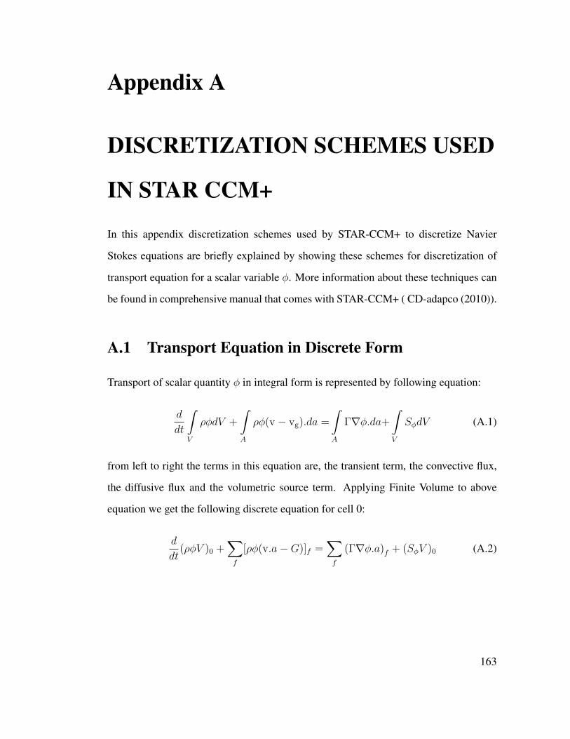
Appendix A
DISCRETIZATION SCHEMES USED
IN STAR CCM+
In this appendix discretization schemes used by STAR-CCM+ to discretize Navier
Stokes equations are briefly explained by showing these schemes for discretization of
transport equation for a scalar variable φ. More information about these techniques can
be found in comprehensive manual that comes with STAR-CCM+ ( CD-adapco (2010)).
A.1 Transport Equation in Discrete Form
Transport of scalar quantity φ in integral form is represented by following equation:
d
dt
∫
V
ρφdV +
∫
A
ρφ(v − vg).da =
∫
A
Γ∇φ.da+
∫
V
SφdV (A.1)
from left to right the terms in this equation are, the transient term, the convective flux,
the diffusive flux and the volumetric source term. Applying Finite Volume to above
equation we get the following discrete equation for cell 0:
d
dt(ρφV )0 +
∑
f
[ρφ(v.a−G)]f =∑
f
(Γ∇φ.a)f + (SφV )0 (A.2)
163
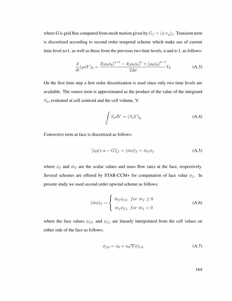
where G is grid flux computed from mesh motion given by Gf = (a.vg)f . Transient term
is discretized according to second order temporal scheme which make use of current
time level n+1, as well as those from the previous two time levels, n and n-1, as follows:
d
dt(ρφV )0 =
3(ρ0φ0)n+1 − 4(ρ0φ0)
n + (ρ0φ0)n−1
2∆tV0 (A.3)
On the first time step a first order discretization is used since only two time levels are
available. The source term is approximated as the product of the value of the integrand
Sφ, evaluated at cell centroid and the cell volume, V:
∫
V
SφdV = (SφV )0 (A.4)
Convective term at face is discretized as follows:
[φρ(v.a−G)]f = (mφ)f = mfφf (A.5)
where φf and mf are the scalar values and mass flow rates at the face, respectively.
Several schemes are offered by STAR-CCM+ for computation of face value φf . In
present study we used second order upwind scheme as follows:
(mφ)f =
mfφf,0 for mf ≥ 0
mfφf,1 for mf < 0(A.6)
where the face values φf,0 and φf,1 are linearly interpolated from the cell values on
either side of the face as follows:
φf,0 = φ0 + s0(∇φ)r,0 (A.7)
164
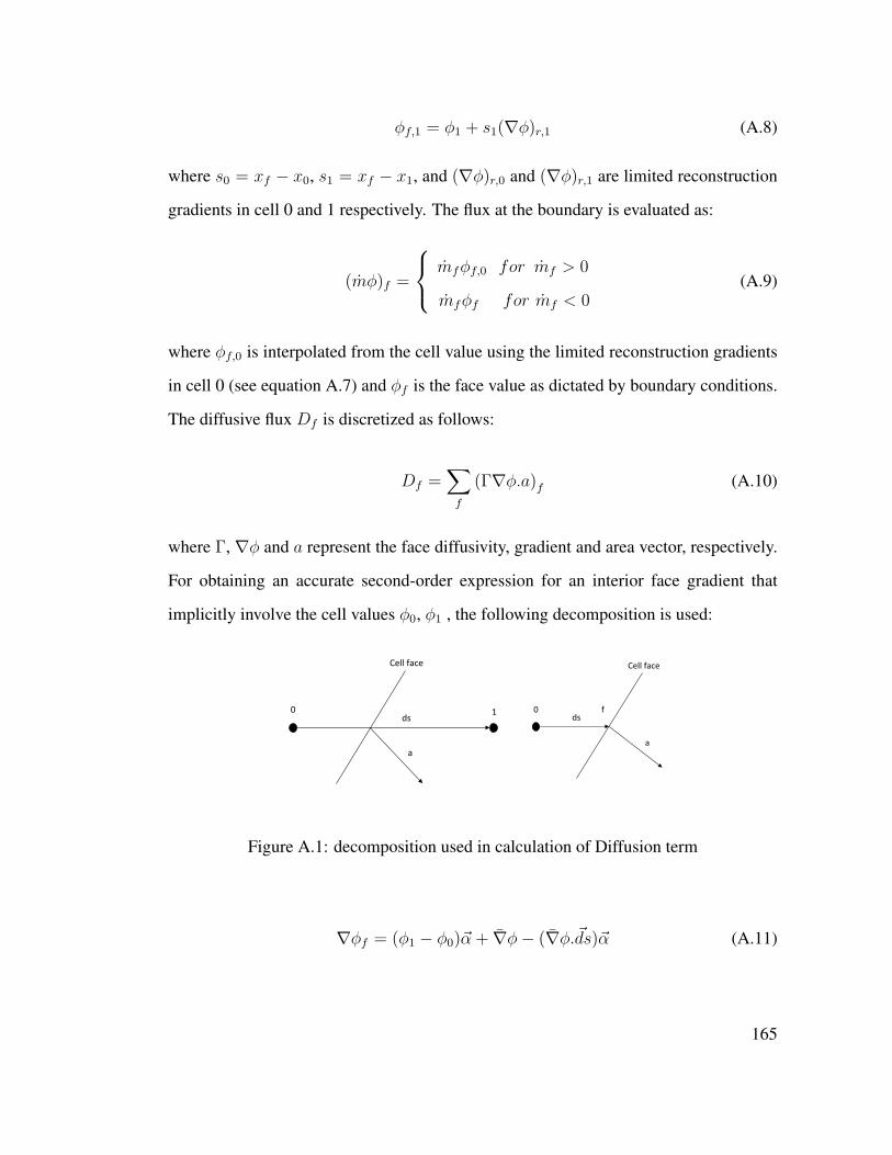
φf,1 = φ1 + s1(∇φ)r,1 (A.8)
where s0 = xf − x0, s1 = xf − x1, and (∇φ)r,0 and (∇φ)r,1 are limited reconstruction
gradients in cell 0 and 1 respectively. The flux at the boundary is evaluated as:
(mφ)f =
mfφf,0 for mf > 0
mfφf for mf < 0(A.9)
where φf,0 is interpolated from the cell value using the limited reconstruction gradients
in cell 0 (see equation A.7) and φf is the face value as dictated by boundary conditions.
The diffusive flux Df is discretized as follows:
Df =∑
f
(Γ∇φ.a)f (A.10)
where Γ, ∇φ and a represent the face diffusivity, gradient and area vector, respectively.
For obtaining an accurate second-order expression for an interior face gradient that
implicitly involve the cell values φ0, φ1 , the following decomposition is used:
Cell face
0
a
1ds
Cell face
0
a
dsf
Figure A.1: decomposition used in calculation of Diffusion term
∇φf = (φ1 − φ0)~α + ∇φ− (∇φ.~ds)~α (A.11)
165
where ~α = ~a
~a.~ds, ~ds = ~x1 − ~x0, and ∇φ = ∇φ0+∇φ1
2. The diffusion flux at an interior
face may be written:
Df = Γf∇φf .a = Γf [(φ1 − φ0)~α.a+ ∇φ.a− (∇φ.~ds)~α.a] (A.12)
where Γf is average value of the cell values. Second term and third term in above equa-
tion represent the secondary gradient or cross diffusion contribution. They are neces-
sary for maintaining accuracy on non-orthogonal meshes. For boundary faces a similar
decomposition is used
Df = Γf∇φf .a = Γf [(φf − φ0)~α.a+∇φ0.a− (∇φ0.~ds)~α.a] (A.13)
where ~ds = ~xf − ~x0. Similar to interior faces the second and third term are cross
diffusion contribution which can be neglected if mesh is orthogonal.
A.2 Gradient Computation
STAR-CCM+ first calculates unlimited reconstruction gradients. Using unlimited
reconstruction gradients direct is problematic because it may in some instances exceed
the cell values bounding the face. For this reason it is necessary to limit reconstruction
gradients by scaling them appropriately in each cell. Once these unlimited reconstruc-
tion gradients are limited they are used to evaluate the cell gradients to reconstruct face
values for flux computations. Unlimited reconstruction gradients for pressure is calcu-
lated using weighted least squares method. In weighted least square method the initial
166
unlimited reconstruction gradients (∇φ)ur in cell 0 are computed using the following
weighted list square formula:
(∇φ)ur =
[∑
f
ds⊗ ds
ds.ds
]−1 [∑
f
(φ0 − φn)ds
ds.ds
]
(A.14)
where ~ds = ~xn − ~x0, and ~x0 and ~xn representing centroid of cell 0 and neighbor cell
addressed through face and φ0 and φn represent the data values in cell 0 and its neigh-
bors. Gauss divergence theorem is used to calculate unlimited reconstruction gradients
for calculation of other variables such as velocity. Gauss divergence theorem states that:
∫
V
∇φdV =
∫
A
φda (A.15)
written in discrete form allows us to compute initial unlimited reconstruction gradients
as:
(∇φ)ur =1
V0
∑
f
φfaf (A.16)
where the face value φf is approximated by the arithmetic average of the adjacent cell
values as φf = φ0+φ1
2. Limited reconstruction gradients for cell 0 are calculated using
the scale factor α as follows:
(∇φ)r,0 = α(∇φ)ur,0 (A.17)
where α = min(αf ) and αf is given by following equation:
αf =2rf + 1
rf (2rf + 1) + 1(A.18)
167
rf is given by:
rf =
∆f
∆maxfor ∆f > 0
∆f
∆minfor ∆f ≤ 0
(A.19)
∆f is given by:
∆f = φf,0 − φ0 = s0(∇φ)ur,0 (A.20)
where:
∆max = φmax0 − φ0 (A.21)
∆min = φmin0 − φ0 (A.22)
For cell 0, φmax0 and φmin
0 quantities can be defined as:
φmax0 = max(φ0, φneighbors) (A.23)
φmin0 = min(φ0, φneighbors) (A.24)
where φneighbors represents the cell values in each neighbor that has a common face with
cell-0. Reconstruction gradients explained in previous section are used for computing
bounded face values from cell values and are used for convective quantities. Cell gradi-
ents are used in many other places such as secondary gradients for diffusive terms and
pressure gradients in pressure-velocity coupling. The improved estimates of face values
obtained from reconstruction gradients can in turn be used to obtain better estimates of
cell gradients. Using Gauss divergence theorem we obtain:
∇φ =1
V0
∑
f
φf (A.25)
168
Where the face value is approximated by arithmetic average of the face values from
adjacent cell values as φf =φf,0+φf,1
2. where φf,0 and φf,1 are obtained using equation
A.7, A.8.
169