Embed Size (px)
Citation preview
UNIVERSITY OF CALIFORNIA SAN DIEGO
Computational Analysis of MEMS biosensor for
Alzheimer’s disease diagnostics
A Thesis submitted in partial satisfaction of the
requirements for the degree Master of Science
in
Engineering Sciences (Engineering Physics)
by
Abhijith Karkisaval Ganapati
Committee in charge:
Professor Ratnesh Lal, Chair
Professor Shengqiang Cai
Professor Padmini Rangamani
2018

Copyright
Abhijith Karkisaval Ganapati, 2018
All Rights Reserved

iii
The Thesis of Abhijith Karkisaval Ganapati is approved and it is acceptable in quality and form
for publication on microfilm and electronically.
________________________________________________________________________
________________________________________________________________________
________________________________________________________________________
Chair
University of California San Diego
2018
iv
TABLE OF CONTENTS
Signature Page……………………………………………………………………………..…..…iii
Table of Contents………………………………………………………………………………....iv
List of Figures…………………………………………………………………………………....vii
List of Tables…………………………………………………………………………………..….x
Acknowledgements……………………………………………………………………………….xi
Abstract of the Thesis………………………………………………………………………….....xii
Introduction ..................................................................................................................................... 1
Chapter 1 ......................................................................................................................................... 5
1.1 Detection Modalities in Alzheimer’s disease ............................................................ 5
1.2 Biosensors as an effective diagnostic tool ................................................................. 6
1.3 Different types of Biosensors ..................................................................................... 7
1.3.1 Fabrication Technology .......................................................................................... 7
1.3.2 Transduction mechanism ........................................................................................ 9
Chapter 2 ....................................................................................................................................... 17
2.1 Theory of Mass Based Resonator Sensors ............................................................... 17
2.1.1 Single-Degree-of-Freedom (SDOF) Systems ....................................................... 17
2.1.2 Free Vibration ....................................................................................................... 18
2.1.3 Harmonically Excited Forced Vibration ............................................................... 19
2.2 Continuous, Multiple Degree of Freedom Systems ................................................. 21
v
2.2.1 Solution for the case of free vibration ................................................................... 23
2.2.2 Harmonically Excited Beam ................................................................................. 24
2.3 Frequency response of structure immersed in fluid ................................................. 24
2.4 Mechanics of mass sensitivity ................................................................................. 26
Chapter 3 ....................................................................................................................................... 28
3.1 Computational Technique – Finite Element Method ............................................... 28
3.2 Fluid- Structure Interaction Problems ...................................................................... 30
3.2.1 Approaches to solving FSI problems .................................................................... 32
3.2.2 Structure coupled with stagnant fluid ................................................................... 35
3.2.3 Transient FSI framework in Ansys Workbench (time domain)............................ 36
Chapter 4 ....................................................................................................................................... 39
4.1 Setup of computational model in ANSYS Workbench ........................................... 39
4.2 Modal Analysis – Extraction of natural frequencies. ............................................... 40
4.3 Harmonic Response Analysis .................................................................................. 43
4.4 Frequency domain analysis in fluid environment .................................................... 43
4.5 Point mass analysis .................................................................................................. 47
4.6 Time domain simulations with flowing fluid........................................................... 48
4.8 Fluid Flow – Fluent setup ........................................................................................ 51
4.9 System Coupling Setup ............................................................................................ 53

vi
Chapter 5 - Results of the simulation ............................................................................................ 55
5.1 Frequency Domain Results: Modal and harmonic response analysis in vacuum .... 55
5.2 Modal and Harmonic response analysis in fluid environment ................................. 58
5.3 Cantilever immersed in liquids of different kinematic viscosities ........................... 60
5.4 Point mass analysis – biomarker attachment ........................................................... 61
5.5 Transient simulation results ..................................................................................... 62
Chapter 6 ....................................................................................................................................... 70
6.1 Conclusions .............................................................................................................. 70
6.2 Future work .............................................................................................................. 72
References: .................................................................................................................................... 73

vii
LIST OF FIGURES
Figure 1 - Different kinds of sensors based on transduction mechanism ......................... 12
Figure 2 - Laser Doppler Vibrometry (LDV) setup .......................................................... 15
Figure 3 - Schematic of the current biosensor design ....................................................... 16
Figure 4 - Optical waveguide schematic for evanescent wave generation ....................... 16
Figure 5 - SDOF Vibration system ................................................................................... 18
Figure 6 - Dynamic amplification factor and phase angle for SDOF system ................... 20
Figure 7 - Schematic of continuous modeling approach for a cantilever beam................ 22
Figure 8 - Schematic showing monolithic and partitioned approaches ............................ 33
Figure 9 – Overview of FSI methods ................................................................................ 34
Figure 10 - Schematic showing extent of physics coupling in different problems ........... 36
Figure 11 - System coupling framework ......................................................................... 37
Figure 12 - Schematic of iterative coupling scheme ......................................................... 38
Figure 13 - Schematic of beam and bimorph piezo strip .................................................. 41
Figure 14 - Mesh generated for microcantilever ............................................................... 42
Figure 15 - Geometry of Acoustics FSI ............................................................................ 44
Figure 16 - Wireframe mesh of the acoustic model .......................................................... 45
Figure 17 - Boundary conditions for acoustic FSI ............................................................ 46
Figure 18 - Transient FSI workflow ................................................................................. 48
Figure 19 - Geometry of Transient FSI setup …………………………………………...49
Figure 20 - Mesh generated for the beam………………………………………………..49
Figure 21- Sinusoidal load applied ................................................................................... 50
Figure 22 – Boundary condition for transient FSI ............................................................ 51
viii
Figure 23 - Fluid domain mesh ......................................................................................... 51
Figure 24 – Data Transfer setup........................................................................................ 53
Figure 25 – Mode shapes in vacuum .............................................................................. ..55
Figure 26 – Frequency response of piezo actuated beam at 5V drive voltage ................. 56
Figure 27 – Comparison of resonance frequencies from AFM and simulation results .... 57
Figure 28 – Modal shapes of microcantilever beam immersed in water .......................... 58
Figure 29 – Frequency response of first vibration mode in water .................................... 59
Figure 30 – Frequency shift under different fluid conditions ........................................... 60
Figure 31 - Shift in the frequency with respect to varying viscosity…………………….60
Figure 32 – Shift in the frequency vs added point mass…………………………………61
Figure 33 – Drag force at FSI interface – Acetone………………………………………63
Figure 34 – Drag force at FSI interface – Water…………………………………………63
Figure 35 – Drag force at FSI interface – ethylene glycol………………………………..63
Figure 36 - Drag force at FSI interface – Acetone……………………………………….64
Figure 37 - Drag force at FSI interface – Water………………………………………….64
Figure 38 - Drag force at FSI interface – ethylene glycol………………………………...64
Figure 39 – Snapshots of velocity contours in mid-plane for various time steps…………66
Figure 40 – Close-up view of pressure contour at the mid-plane………………………...67
Figure 41 – Close-up view of velocity contour at the mid-plane…………………………67
Figure 42 – 3D flow velocity vectors in the computational domain……………………..68

ix
Figure 43 – Flow perturbation at the free end of the cantilever………………………….69

x
LIST OF TABLES
Table 1 – Model Biomarker system…………. ……………………………………..….47
Table 2 - Natural frequencies of the piezo actuated beam in vacuum……………..…...56
Table 3 – Comparison of results for the model system…………………………….…...57
Table 4 - Natural frequencies of microcantilever beam immersed in water……..…,….58
Table 5 – Drag force assessment for fluid case 1 – along thickness dimension………..63
Table 6 – Drag force assessment for fluid case 2 – along width dimension………...….64

xi
ACKNOWLEDGEMENTS
I would like to thank my advisor Prof. Ratnesh Lal for his continuous support and guidance
throughout the course of the project. I would also like to thank the committee members
Prof. Shengqiang Cai and Prof. Padmini Rangamani for fruitful advice and suggestions in the
successful completion of the project.
I would like to thank the members of Lal lab: Deependra Kumar Ban, Joon Lee, Michael
Hwang Juan Ybarra, Vrinda Sant, Qingqing Yang, Nirav Patel, Grace Jang, Madhura Som,
Yushuang Liu, Jay Sheth for all the healthy discussions, insightful advice and creating an
atmosphere in the lab that promotes research and scientific thinking.
I would especially like to thank my family and friends who were a source of continuous
motivation and emotional support during the times I needed them the most.
I would like to thank Elsevier publications and John Wiley and Sons publications for
permitting me to use figures which helped in shaping this thesis. Last but not the least, I would
like to thank all the faculty members and staff of MAE department and UCSD for letting me be a
part of this wonderful community.
xii
ABSTRACT OF THE THESIS
Computational Analysis of MEMS biosensor for
Alzheimer’s disease diagnostics
by
Abhijith Karkisaval Ganapati
Master of Science in Engineering Sciences (Engineering Physics)
University of California San Diego, 2018
Dr. Ratnesh Lal, Chair
Alzheimer’s disease (AD) is an incurable, debilitating neurodegenerative disease affecting
millions of elderly people worldwide. Though the exact mechanism of the causation of the disease
still remains unknown, early diagnostic methods can certainly help in pinpointing the timeline and
xiii
progression of the disease. In this regard, biomarker sensors are reliable candidates which provide
quicker analysis times and accurate diagnosis. Mass based micro-electromechanical systems
(MEMS) biosensors, with increasing versatility and functionality are being radically implemented
in biomedical device industry. A thorough understanding of the mechanics and dynamics of the
biosensor under various operating conditions are absolutely essential to predict and improve the
performance of the biosensor. A MEMS biosensor incorporating mass based resonance frequency
shift detection and evanescent wave based fluorescence signal detection achieves dual mode of
detection and higher reliability. In this thesis, a finite element based computational approach
including fluid-structure interaction is developed for the sensor geometry and the dynamics of the
sensor under various fluid conditions and damping mechanisms are explored. Spatially localized
parameterized point masses are attached to simulate the effect of biomarker attachment to the beam
sensing surface and frequency response of the sensor is analyzed. Monolithic and partitioned
approaches for solving coupled physics problems are designed and analyzed. The results obtained
from finite element simulations are compared against experimental data obtained from AFM
calibration measurements and analytical model. Some approaches towards optimization of the
performance of the biosensor with real world clinical applications are also explored.
Keywords: Finite Element Analysis, Fluid-structure interaction, MEMS, Alzheimer’s disease
1
Introduction
Alzheimer’s disease (AD) is an irreversible neurodegenerative disorder affecting the
central nervous system, leading to progressive loss of memory, functional decline and ability to
learn, interfering with a person’s daily life and activities. Alzheimer’s is the leading cause of
dementia among older adults, currently being regarded as the sixth leading cause of death in the
United States and an estimated 5 million Americans are living with Alzheimer’s [1]. Future
estimates show that by the year 2050, worldwide, the number of people affected by the disease is
going to dramatically increase to a million cases per year [2]. Although some of the drugs available
to handle the disease seem to relieve the symptoms and stunt the progression, an exact cure remains
a distant reality. This has to do with the fact that, the intricate mechanism of the cause of the disease
remains a mystery, only the neuropathological features being pointers in the diagnosis. As the
major demographic affected by the disease are elderly people, the symptoms are harder to notice
early on and are generally noticeable when the disease has progressed beyond control.
The classic features of Alzheimer’s disease include the presence of extracellular deposits
in the brain tissue called Amyloid plaques (Aβ), neurofibrillary tangles (NFT), increase in
oxidative stress, and changes in the brain structure which are normally revealed through brain
imaging modalities. Amyloid plaques consist of the fragments of the protein amyloid beta which
mainly originates through a precursor molecule called amyloid precursor protein (APP).
Neurofibrillary Tangles consist of hyper phosphorylated Tau proteins. While Tau proteins are
integral for maintaining nerve cell structure and health, the excessive phosphorylation seems to
contribute towards formation of NFTs [3]. Oxidative stress, a resultant of formation of oxygen free
radicals due to imbalance in redox reactions, causing cellular toxicity is also regarded as one of
the hallmarks of the disease [4]. Reduction in volume of the brain, atrophy of certain distinct
2
regions of the brain have also been regarded as potential indicators. In addition to these classic
symptoms, other symptoms generic to other forms of dementia may also be present. An accurate
assessment of these characteristics is an active area of research in AD.
Many hypotheses have been proposed in order to explain the causation of AD. The
cholinergic hypothesis, one of the earliest proposed, argues that a reduction in the synthesis of
acetylcholine – a neurotransmitter, as the cause of the disease. However, this hypothesis has
struggled to maintain its stand mainly because of failure of therapies concentrated towards
improving acetylcholine synthesis [5]. The amyloid hypothesis proposed in 1991, postulates that
amyloid beta (Aβ) deposits are the fundamental cause of the disease. Accumulation of Aβ deposits,
improper breakdown and removal of amyloid beta by apolipoprotein (APOE4 – lipoprotein
responsible for breakdown, removal and maintaining Aβ levels in the brain tissue) are some key
points put forward by the amyloid hypothesis. This hypotheses was updated in 2009 proposing
that a close analog of Aβ protein may play the major role in the neuronal degradation. The theory
suggested that amyloid-related mechanisms that were responsible for maintaining neuronal health
in early stages of life may be affected due to ageing related processes and blocked molecular
pathways, ultimately failing to regulate neuronal conditions and thus paving way for AD
progression [6]. Although the amyloid hypothesis has been a leading candidate in explaining AD
causation and progression, recent clinical trials of drugs manufactured on the basis of conclusions
derived from the hypothesis, have not been successful in halting the progression of the disease [7].
Another contemporary, well known hypothesis is the Tau hypothesis which posits that hyper
phosphorylated Tau protein abnormalities are fundamental to the triggering of the disease. When
neurofibrillary tangles formed by tau proteins inside neuronal cells starts destroying the
microtubules, cell function is compromised and neuronal transport system is disrupted, eventually
3
leading to irregularities in biochemical signaling and transport and death of cells [8, 9, and 10].
Neurovascular hypothesis proposes that problems with cellular homeostasis of metallic elements
like ionic copper, iron and zinc is poorly regulated in AD and the compromised functioning of
blood brain barrier might also be a contributor. These ions affect tau, apolipoproteins and amyloid
precursor proteins which might in turn lead to dysregulation of oxidative stress and toxic radicals,
thus enabling a cascade of events which ultimately lead to AD progression [11, 12]. Some other
theories proposed take into consideration dysfunction of oligodendrocytes as the main cause and
production of tau, Aβ as side effects [13]. Retrogenesis, as a medical hypothesis has been
suggested which takes into account the reverse neurodegeneration process starting with death of
axons and ending with degradation of grey matter cells in the brain [14]. Hence, a lot of research
work is in progress towards understanding more about AD, its causation and possible therapeutics.
Chapter 1 consists of a review of detection modalities for Alzheimer’s biomarkers, the role
of biosensors in effective diagnostics, the different types of biosensors available depending on
quantities of interest, brief working mechanisms and constraints. Higher emphasis is laid on mass
based MEMS sensors and fabrication of sensors for point of care diagnostics which is a key topic
of the thesis.
Chapter 2 outlines fundamental concepts concerning the mechanics of mass based sensors
delving into solid mechanics, fluid mechanics, theory of vibration, fluid-structure interaction (FSI),
and energy dissipation mechanisms in MEMS sensors.
Chapter 3 outlines computational methods to understand the design and performance of
these sensors under different configurations, concepts in finite element analysis, multiphysics
coupled problems, strategies for solving FSI problems, frequency domain and time domain
methods, vibroacoustic techniques and solver strategies.
4
Chapter 4 outlines the setup of the computational model in the finite element solver
ANSYS, the constraints and boundary conditions applied for sensor geometries, loads applied and
results extracted.
Chapter 5 outlines the results obtained from the finite element methods and comparison
with AFM measurements, analytical models and discussion of the results.
Chapter 6 includes conclusions derived from the work and possible future directions
towards improvement in the design and performance of MEMS biosensors.
5
Chapter 1
1.1 Detection Modalities in Alzheimer’s disease
Early stage definitive diagnosis of AD is extremely difficulty unless significant loss of
cognitive functions is reported. Mental testing and medical history analysis are used as standard
protocols followed by brain imaging techniques. Single photon emission computed tomography
(SPECT) has proven to be a reliable imaging technique with the capability to differentiate AD
from other forms of dementia [15]. Positron Emission Tomography (PET) with radionuclide
tracers is widely used to detect Aβ deposits with high accuracy. With the development of effective
radionuclide tracers, higher reliability is being achieved in AD diagnosis through PET scanning.
Detection of Aβ peptides in the brain is always used in conjunction with other biomarkers for
higher diagnostic efficiency and reducing the amount of false positives. For example Magnetic
Resonance Imaging of the brain is also carried out to check for volumetric shrinkage in the
atrophied regions of the brain [16].
All the current available methods require the use of high end equipment which are available
only in medical institutions or research facilities. The diagnosis procedure is time consuming and
obviously very expensive, without even getting into the treatment side of things. Hence, a lot of
research effort is being invested into early diagnosis of Alzheimer’s disease to avoid the potential
progression or to get a better handle on the future treatment options. In this regard, biosensors are
being developed which have the capability to detect biomarkers associated with AD. Potential
biomarkers for AD are rapidly being discovered which can provide an estimate of the degree of
AD progression, cognitive impairment or brain matter degradation.
6
1.2 Biosensors as an effective diagnostic tool
A biomarker can be a physiological, biochemical or anatomic traceable substance that gives
an indication of the specific hallmarks of disease related parameters. Judgments can be made on
the basis of the presence of the biomarker, or absence thereof, the specific amount of the biomarker
present or the interaction of the biomarker with a test substance or system. A sensing element can
be specially designed to capture and quantify individual biomarkers, leading to quick and reliable
detection. An ideal diagnostic biomarker should provide high degree of specificity with the test
target and help in predicting the pathological condition up to a reasonable degree. The
corresponding sensing element has to be chosen carefully such that it picks up only the biomarker
of interest from a pool of analyte which might possibly contain other biomarkers, media fluid,
impurities and many unwanted substances. This process of choosing the biomarkers and sensing
element pair has to be designed carefully to ensure high affinity of the biomarker with the sensor.
Failing to do this, might lead to spurious, inconclusive measurements.
The fundamental components of a biosensor are: a sensitive biological element, a
transducer and a signal processor. Depending on the chosen modality of transduction, appropriate
signal conditioning methods are applied. These biosensors are fabricated at crossroads of many
scientific fields such as biology, physical chemistry, mechanics, electronics, optics, semiconductor
manufacturing technology etc.,
Some characteristics expected of a biosensor are:
1) Easy to fabricate, scalable technology
2) Inexpensive
3) Easy to use, with minimum or no training(Ideal for point of care testing devices)
4) Fast, efficient and quality readout
7
5) Capable of performing multiple assays with little modification
The following section gives a brief description of different kinds of biosensors designed and their
relative advantages.
1.3 Different types of Biosensors
Biosensor variability mainly arises from the end use application, signal transduction
mechanism and fabrication technologies used. The end use applications may range from detection
of particulate matter in air, pollutant level assessment in air, cell mechanics, rheological
measurements, pathogen detection in food materials, biomarker/biomolecule detection, disease
diagnostics, macromolecule detection, energy harvesting etc., Transduction mechanism refers to
the type of detection scheme used in terms of physical and signal acquisition aspects of the system.
Fabrication technology decides the materials used in the construction of the device, techniques
used to achieve the intended design, functionality and scalability.
1.3.1 Fabrication Technology
As most of the end use applications mentioned above involve targets whose length scales
are in the range of micrometers to angstroms, miniaturized analysis systems serve as the best bet
in detection of these targets. It’s a general rule of thumb that best sensitivity or efficiency is
achieved when the system analyzing the target is at a similar mass scale as that of the target. Hence,
Microelectromechanical Systems (MEMS) structures have been utilized in this regard and have
been proven to be highly effective with their sensing behavior. MEMS are micron sized devices
with one or more moving components which form the heart of the system. MEMS are made of
components whose size ranges from a micrometer to several hundred micrometers, which also
implies that the target volume interacting with the sensing element is very less, thus providing
8
sensing capabilities with limited sample availability and sometimes without the need of sample
amplification. Due to their miniature size, very high surface area to volume ratios are achieved.
Surface chemistry principles weigh in during the manufacture and functioning of the device. The
fabrication of MEMS devices borrows the technology know how from semiconductor processing
and microelectronics manufacturing industries. Basic techniques involving deposition of material
layers, patterning of specific shapes and geometries using photolithography and etching are
standard operating procedures during the fabrication of MEMS devices. Silicon based materials
have formed the majority of MEMS applications due to their ease of processing, very high
scalability and device reproducibility with little to no errors. Silicon based materials exhibit low
energy dissipation with very good signal to noise ratio. Semiconducting property of silicon is
another added advantage that is highly used in electronics based sensors and devices.
Polymers are also among highly used materials in MEMS industry as they can be produced
in high volumes covering a wide range of material and mechanical characteristics. Few metals
such as gold, silver, platinum, copper, chromium, titanium etc., are used for applications which
desire superior mechanical properties and reliability. Ceramics are another class of materials that
are increasingly being tested and used in MEMS and sensor research as they offer few advantages
that result from combination of materials. Nitrides and carbides of silicon, aluminum, and tungsten
offer multiple characteristics such as better mechanical properties, piezoelectric, piezoresistive,
pyroelectric properties which are often helpful in increasing the multitude of functionality of a
device. Often materials used for fabrication of biosensors have to be operated in different kinds of
environment (gases and liquids). Hence it is important to choose a material that offers resistance
to degradation in different environments, without compromising sensor characteristics.
9
Most MEMS devices used in biosensor applications follow fabrication methods derived
from semiconductor manufacturing processes. Thin films of the material are deposited on a
substrate using physical or chemical vapor deposition techniques. A pattern is transferred onto the
deposited film on the substrate in a process called lithography. Optical (photolithography), electron
beam or ion beam lithography techniques are generally used to transfer the pattern. After the
pattern is transferred, an etching step is used to remove the undesired material in the geometry.
Wet and dry etching methods are available which remove the excess material based on immersion
in a liquid etchant solution or a vapor phase etchant (sometimes charged ions). Finally a die
separation method is employed to reduce the wafer thickness and separate the device from the
substrate [38].
1.3.2 Transduction mechanism
Electrical transduction involves gathering data about a sensing event based on a measurable
electrical signal. Biological or chemically active sensing elements are coupled to an electrode
transducer. In an event of sensing, the binding of the target to the active sensing elements causes
a change in the electrical properties of the electrode or causes a change in the signal characteristics
of the electrode which can be precisely quantified. Electrochemical biosensors are mainly
classified into four types: i) Amperometric biosensors – sensing event causes a change in the
electric current passing through the electrodes (redox reactions at the electrode) ii) Conductometric
biosensors – sensing event causes a change in conductance between reference electrodes which
can be measured. iii) Potentiometric biosensors – sensing event causes a change in the electrode
voltage potential due to ions involved in the process, iv) Impedimetric biosensors – sensing event
causes a change in the electrochemical impedance properties. DNA hybridization detection with
high accuracy has been achieved using amperometric detection technique [17]. Single nucleotide
10
polymorphism (SNP) detection has been successfully carried out which mainly used amperometric
techniques with nucleotides that were modified to function as electrochemical probes [18, 19]. By
integrating transistor technology to electrochemical detection, potentiometric biosensors sense the
change in voltage between the source and drain electrodes. Ion-sensitive Field Effect Transistors
(ISFETs), Graphene Field Effect Transistors(GFETs), Complementary Metal Oxide
Semiconductor (CMOS-ISFETs) are being heavily used for precise electrochemical quantification.
Some applications include SNP detection in DNA [20], Label free hybridization detection in DNA
[21], monitoring of cellular activities like respiration and acidification [22].
Conductometric biosensors provide an estimate of the ionic strength in the electrolytes and
have been used to detect various analytes such as urea, glucose, biochemicals and toxic materials
[23, 24]. Surface modified electrodes can be used in the analysis of impedance, combining the
analysis of resistance and capacitive changes as functions of frequency of the operating signal
between the electrodes in an impedometric biosensor. Immunosensors based on this principle have
been used to detect prostate-specific antigen (PSA) [25], atrazine biosensor based on magnetic
nanoparticles in conjunction with impedometric measurements [26].
Optical biosensors utilize a change in optical signal as their basic transduction mechanism.
This optical signal maybe a change in an optical property such as refractive index, absorption or
reflection of an optical signal, change in optical path, total internal reflection, fluorescence and
chemiluminescence. Fluorescence signal based optical biosensors are the most common in
biological applications because of their high reliability, high spatial resolution and wide range of
targets covered. Another significant advantage of fluorescence based optical transducers is that the
theoretical resolution may reach up to single molecule level. The detection probe which is
11
immobilized on a surface is attached with a fluorescent marker molecule. When the target molecule
attaches to the probe, a change in the fluorescent signal intensity is measurable. The fluorescent
markers absorb and emit light at specific wavelengths. This difference in absorbance and emission
peaks of marker molecules, termed as Stoke’s shift, enables these biosensors to perform efficient
detection. Wide range of fluorescent biomarkers are available with varying degrees of Stoke’s
shift, suitable for different applications. Fluorescence Resonance Energy Transfer (FRET) is a
technique popularly used in biological sensors, wherein attachment of a target molecule to the
probe molecule can be detected either through the reduction in fluorescence intensity of the
fluorescently tagged probe with time, or an increase in the fluorescence intensity with time.
Chemiluminescence is the emission of energy in the form of measurable light in the event of a
chemical binding reaction. Whenever a target binds to the probe through a chemical reaction,
energy is released in the form of light which is measurable and quantifiable. In some organisms
this phenomena happens naturally and is termed as bioluminescence. Artificially induced
luminescence techniques called electrochemiluminescence, can be achieved through passage of
electrical current through the probes.
The geometric construction of the optical platform is a critical factor in the proper
functioning of optical devices. Hence, many approaches have been implemented taking into
careful consideration of geometrical aspects. Microarray technology is one such example where in
a substrate usually made of silicon, is modified to construct specific sites where fluorescently
tagged probe molecules can be immobilized in very high numbers. When a target analyte is
introduced on the substrate, binding events are indicated through change in fluorescence signals.
Optical signal detection systems are integrated to the microarray chips, such that quick readout of
the optical signals are performed and a software quickly indicates site specific information. This
12
technology has been commercialized and implemented at large scale for genetic information
extraction, SNP and methylation detection in DNA etc., [27, 28, and 29]. Waveguide based
biosensors are an interesting category of optical biosensors which offer integration of multiple
functionalities in a chip. Total Internal Reflection Fluorescence (TIRF) waveguide systems utilize
TIR phenomena to couple a laser beam into the waveguide, which total internally reflects in the
waveguide geometry. Due to this reflection, evanescent waves which exponentially decay in
intensity form at the interface of waveguide and external medium. This evanescent wave can be
used to detect fluorescence at a very small scale, thus providing high nearfield spatial resolution.
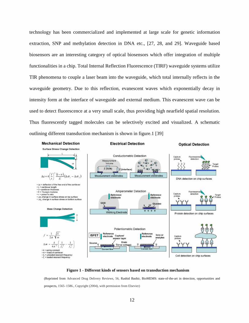
Thus fluorescently tagged molecules can be selectively excited and visualized. A schematic
outlining different transduction mechanism is shown in figure.1 [39]
(Reprinted from Advanced Drug Delivery Reviews, 56, Rashid Bashir, BioMEMS: state-of-the-art in detection, opportunities and
prospects, 1565–1586., Copyright (2004), with permission from Elsevier)
Figure 1 - Different kinds of sensors based on transduction mechanism
13
Mechanical detection as a transduction mechanism has been explored recently and
promises a reliable technique in the field of biomarker detection due to its ease of use with
relatively simple or no sample preparation. Sensor elements can be specially designed for a
particular biomarker purely on the basis of varying mass scales of the biomarkers. Sensing
elements can be functionalized with a large variety of biological elements such as antibodies,
proteins, enzymes etc, such that the corresponding biomarkers attach onto them. This attachment
adds extra mass to the sensing element, thus changing the static or dynamic mechanical properties
of the sensing element. This change can be detected through external means and specific mass
attached can be quantified. With proper choice of biological functionalization agents, highly
sensitive binding events can be detected with high precision. MEMS beams, quartz crystal
microbalance are some of the devices which work on the principle of mechanical detection.
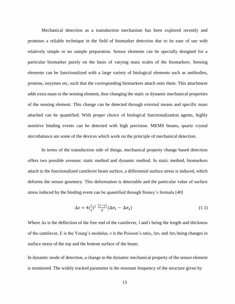
In terms of the transduction side of things, mechanical property change based detection
offers two possible avenues: static method and dynamic method. In static method, biomarkers
attach to the functionalized cantilever beam surface, a differential surface stress is induced, which
deforms the sensor geometry. This deformation is detectable and the particular value of surface
stress induced by the binding event can be quantified through Stoney’s formula [40]
∆𝑧 = 4(𝑙
𝑡)2
(1−𝜈)
𝐸(∆𝜎1 − ∆𝜎2) (1.1)
Where Δz is the deflection of the free end of the cantilever, l and t being the length and thickness
of the cantilever, E is the Young’s modulus, ν is the Poisson’s ratio, Δσ1 and Δσ2 being changes in
surface stress of the top and the bottom surface of the beam.
In dynamic mode of detection, a change in the dynamic mechanical property of the sensor element
is monitored. The widely tracked parameter is the resonant frequency of the structure given by
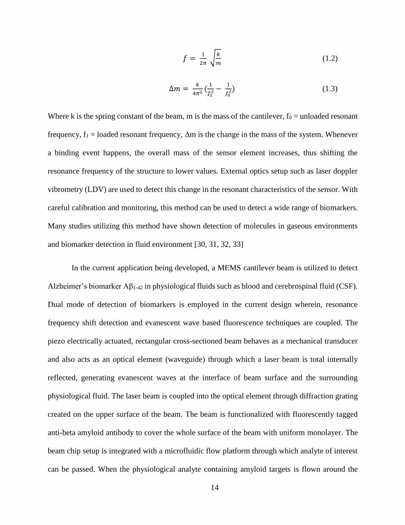
14
𝑓 = 1
2𝜋 √
𝑘
𝑚 (1.2)
∆𝑚 = 𝑘
4𝜋2(
1
𝑓12 −
1
𝑓02) (1.3)
Where k is the spring constant of the beam, m is the mass of the cantilever, f0 = unloaded resonant
frequency, f1 = loaded resonant frequency, Δm is the change in the mass of the system. Whenever
a binding event happens, the overall mass of the sensor element increases, thus shifting the
resonance frequency of the structure to lower values. External optics setup such as laser doppler
vibrometry (LDV) are used to detect this change in the resonant characteristics of the sensor. With
careful calibration and monitoring, this method can be used to detect a wide range of biomarkers.
Many studies utilizing this method have shown detection of molecules in gaseous environments
and biomarker detection in fluid environment [30, 31, 32, 33]
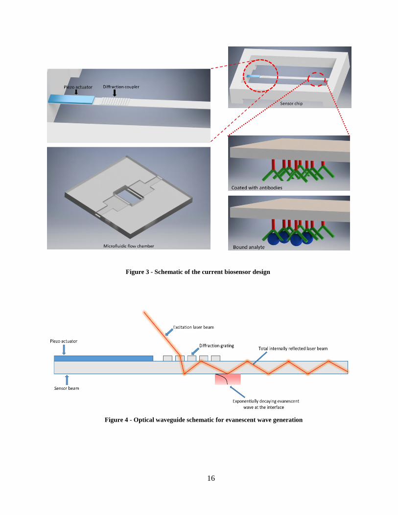
In the current application being developed, a MEMS cantilever beam is utilized to detect
Alzheimer’s biomarker Aβ1-42 in physiological fluids such as blood and cerebrospinal fluid (CSF).
Dual mode of detection of biomarkers is employed in the current design wherein, resonance
frequency shift detection and evanescent wave based fluorescence techniques are coupled. The
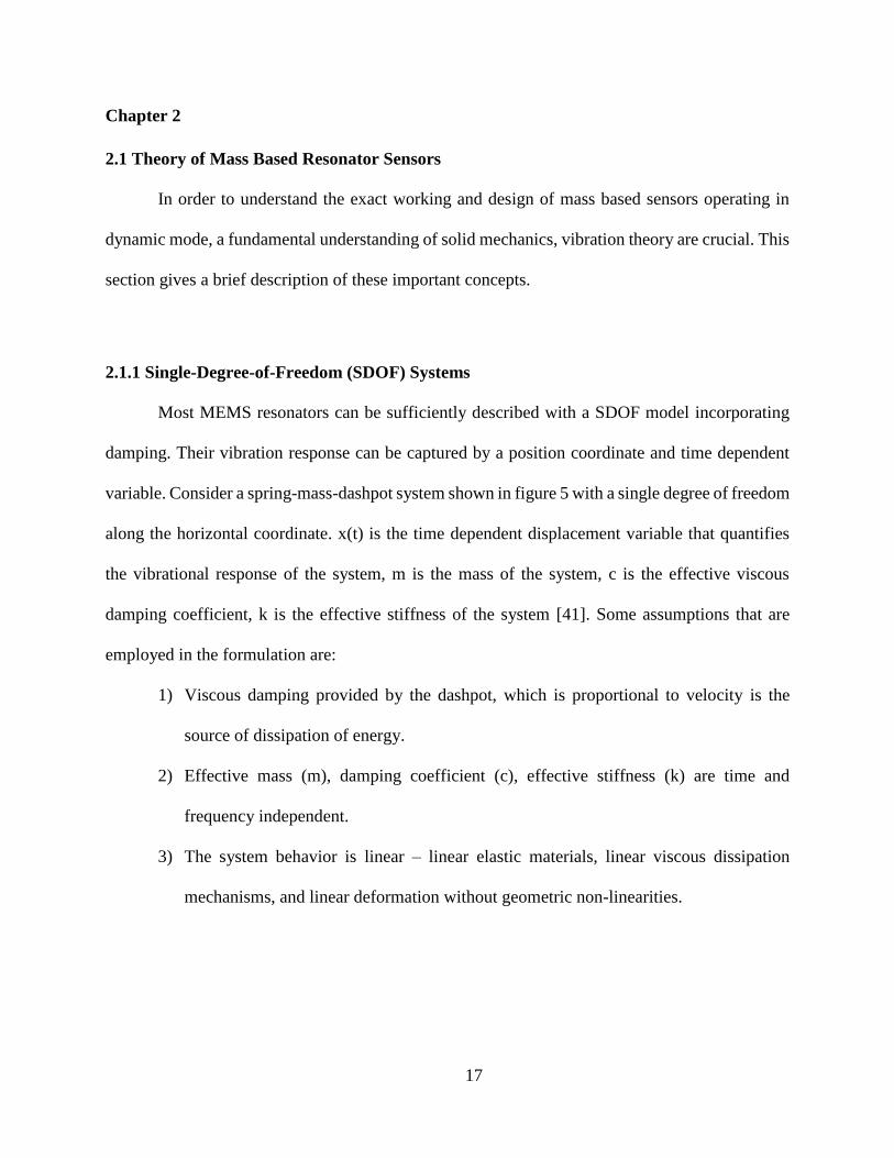
piezo electrically actuated, rectangular cross-sectioned beam behaves as a mechanical transducer
and also acts as an optical element (waveguide) through which a laser beam is total internally
reflected, generating evanescent waves at the interface of beam surface and the surrounding
physiological fluid. The laser beam is coupled into the optical element through diffraction grating
created on the upper surface of the beam. The beam is functionalized with fluorescently tagged
anti-beta amyloid antibody to cover the whole surface of the beam with uniform monolayer. The
beam chip setup is integrated with a microfluidic flow platform through which analyte of interest
can be passed. When the physiological analyte containing amyloid targets is flown around the
15
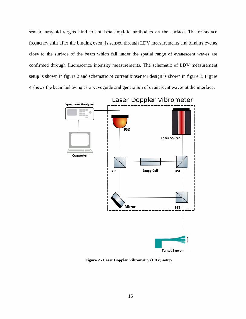
sensor, amyloid targets bind to anti-beta amyloid antibodies on the surface. The resonance
frequency shift after the binding event is sensed through LDV measurements and binding events
close to the surface of the beam which fall under the spatial range of evanescent waves are
confirmed through fluorescence intensity measurements. The schematic of LDV measurement
setup is shown in figure 2 and schematic of current biosensor design is shown in figure 3. Figure
4 shows the beam behaving as a waveguide and generation of evanescent waves at the interface.
Figure 2 - Laser Doppler Vibrometry (LDV) setup
16
Figure 3 - Schematic of the current biosensor design
Figure 4 - Optical waveguide schematic for evanescent wave generation
17
Chapter 2
2.1 Theory of Mass Based Resonator Sensors
In order to understand the exact working and design of mass based sensors operating in
dynamic mode, a fundamental understanding of solid mechanics, vibration theory are crucial. This
section gives a brief description of these important concepts.
2.1.1 Single-Degree-of-Freedom (SDOF) Systems
Most MEMS resonators can be sufficiently described with a SDOF model incorporating
damping. Their vibration response can be captured by a position coordinate and time dependent
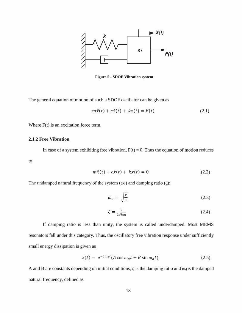
variable. Consider a spring-mass-dashpot system shown in figure 5 with a single degree of freedom
along the horizontal coordinate. x(t) is the time dependent displacement variable that quantifies
the vibrational response of the system, m is the mass of the system, c is the effective viscous
damping coefficient, k is the effective stiffness of the system [41]. Some assumptions that are
employed in the formulation are:
1) Viscous damping provided by the dashpot, which is proportional to velocity is the
source of dissipation of energy.
2) Effective mass (m), damping coefficient (c), effective stiffness (k) are time and
frequency independent.
3) The system behavior is linear – linear elastic materials, linear viscous dissipation
mechanisms, and linear deformation without geometric non-linearities.
18
The general equation of motion of such a SDOF oscillator can be given as
𝑚�̈�(𝑡) + 𝑐�̇�(𝑡) + 𝑘𝑥(𝑡) = 𝐹(𝑡) (2.1)
Where F(t) is an excitation force term.
2.1.2 Free Vibration
In case of a system exhibiting free vibration, F(t) = 0. Thus the equation of motion reduces
to
𝑚�̈�(𝑡) + 𝑐�̇�(𝑡) + 𝑘𝑥(𝑡) = 0 (2.2)
The undamped natural frequency of the system (ω0) and damping ratio (ζ):
𝜔0 = √𝑘
𝑚 (2.3)
𝜁 =𝑐
2√𝑘𝑚 (2.4)
If damping ratio is less than unity, the system is called underdamped. Most MEMS
resonators fall under this category. Thus, the oscillatory free vibration response under sufficiently
small energy dissipation is given as
𝑥(𝑡) = 𝑒−𝜁𝜔0𝑡(𝐴 cos𝜔𝑑𝑡 + 𝐵 sin𝜔𝑑𝑡) (2.5)
A and B are constants depending on initial conditions, ζ is the damping ratio and ωd is the damped
natural frequency, defined as
Figure 5 - SDOF Vibration system
19
𝜔𝑑 = 𝜔0 √1 − 𝜁2 (2.6)
Damped natural frequency is smaller than the undamped natural frequency. For small values of ζ
(<0.2), the difference between ωd and ω0 is negligible.
Another parameter quantifying energy dissipation in oscillatory systems is Quality factor
(Q) in terms of damping ratio, given as:
𝑄 =1
2𝜁=
√𝑘𝑚
𝑐 (2.7)
Larger values of Q indicate the energy dissipation in the system is low and oscillatory response is
sustained for a long duration. A damping ratio of 10% corresponds to decrease in amplitude of the
vibration to half of its initial value in one cycle of vibration.
2.1.3 Harmonically Excited Forced Vibration
In this case the external forcing term F(t) is non zero. The body is excited by an external
force with amplitude F0 and frequency ω. The equation of motion is given as
𝑚�̈� + 𝑐�̇� + 𝑘𝑥 = 𝐹0 sin𝜔𝑡 (2.8)
The steady state solution of the above equation is given as
𝑥(𝑡) = 𝐹0
𝑘𝐷(𝑟, 𝜁) sin[𝜔𝑡 − 𝛳(𝑟, 𝜁)] (2.9)
Where
𝐷(𝑟, 𝜁) = 1
√(1−𝑟2)2+(2𝜁𝑟)2 (2.10)
𝛳(𝑟, 𝜁) = arctan (2𝜁𝑟
1−𝑟2) (2.11)
𝑟 = 𝜔
𝜔0 (2.12)
20
F0/k is the quasi static displacement amplitude, D is defined as the dynamic amplification factor.
ϴ quantifies the phase lag between displacement and force, r is the frequency ratio. When ω = ω0
, this condition is called resonance. The resonance frequency is given as
𝜔𝑟𝑒𝑠 = 𝜔0√1 − 2𝜁2 (2.13)
Thus, resonance frequency is less than damped natural frequency, which is lesser than
undamped natural frequency. The value of dynamic magnification factor at resonance is maximum
and given by
𝐷𝑚𝑎𝑥 = 1
2𝜁√1−𝜁2 (2.14)
Thus, in the absence of any damping, the displacement amplitude goes to infinity. But all
real systems have some degree of damping built into them, thus D never quite reaches infinity. In
real systems, condition of resonance is reached when driving force matches with the system’s
natural frequency. Dmax occurs when r =1 and is given by
𝐷𝑚𝑎𝑥 = 1
2𝜁= 𝑄 (2.15)
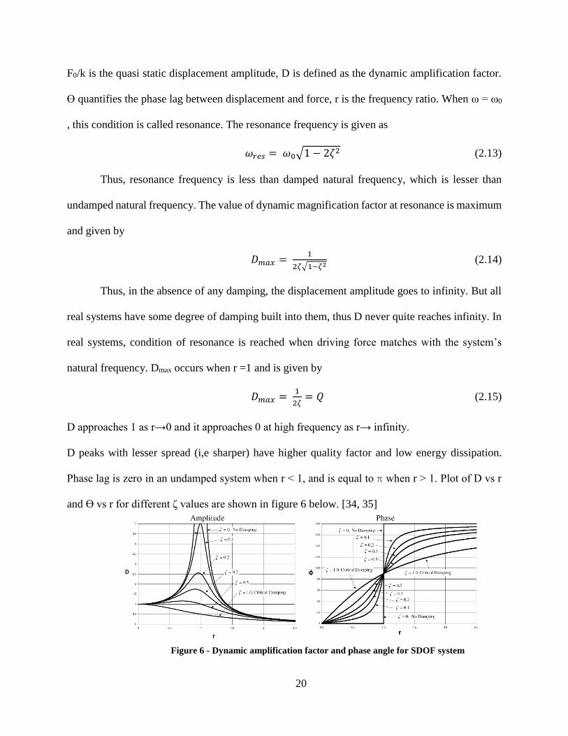
D approaches 1 as r→0 and it approaches 0 at high frequency as r→ infinity.
D peaks with lesser spread (i,e sharper) have higher quality factor and low energy dissipation.
Phase lag is zero in an undamped system when r < 1, and is equal to ℼ when r > 1. Plot of D vs r
and ϴ vs r for different ζ values are shown in figure 6 below. [34, 35]
Figure 6 - Dynamic amplification factor and phase angle for SDOF system
21
2.2 Continuous, Multiple Degree of Freedom Systems
Even though SDOF systems serve as a good starting point in explaining the physics of the
system, most real system require a multiple degree of freedom approach to pin point the exact
behavior. Multiple degrees of freedom capture the dynamics of the system much more accurately.
In one of the approach of modeling MDOF systems, termed as lumped properties or discrete-
coordinate approach, inertial and stiffness properties are assumed to be uncoupled, domains which
have masses associated with them are assumed to be rigid, and domains which are flexible are
assumed to be massless. Finite Element Method (FEM) makes use of this approach, wherein
properties are lumped at nodes of the discrete domain. A resultant system of ODEs is solved to
extract the quantity of interest.
Another approach used to model MDOF systems termed as continuous modeling approach
assumes properties of the system are distributed in the whole domain and not lumped in discrete
points. This type of approach consists of an infinite number of degrees of freedom. Thus a system
of PDEs have to be solved in order to extract the quantities of interest. The system of resonant
biosensor explored in this thesis concerns cantilever and fixed-fixed beam systems. Hence a
continuous modeling approach with cantilever as a system is explained. The analysis can be
extended to beams of various boundary types with just changes in boundary conditions [41].
Common assumptions employed in modeling of beams are:
Mass and stiffness of the beams are time and frequency independent.
The cross-section of the beam is uniform along the length.
Beams have axis of symmetry and vibrations occur along this axis.
Materials considered for the beams are isotropic, linear, elastic and non-linear beam
deformations are not considered.
22
Assumptions of Euler – Bernoulli beam theory apply, cross section of the beam remains
planar during the deformation and remains normal to the deformed beam axis (no
transverse shear strain)
Long and slender beams are considered (length of the beam (L) >> width (b) and height
(h))
Damping is not considered in the general formulation.[49]
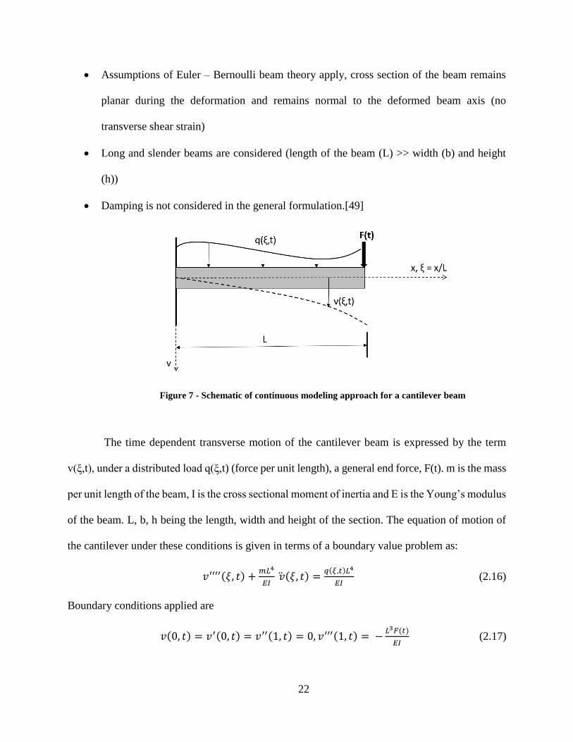
The time dependent transverse motion of the cantilever beam is expressed by the term
v(ξ,t), under a distributed load q(ξ,t) (force per unit length), a general end force, F(t). m is the mass
per unit length of the beam, I is the cross sectional moment of inertia and E is the Young’s modulus
of the beam. L, b, h being the length, width and height of the section. The equation of motion of
the cantilever under these conditions is given in terms of a boundary value problem as:
𝑣′′′′(𝜉, 𝑡) +𝑚𝐿4
𝐸𝐼 �̈�(𝜉, 𝑡) =
𝑞(𝜉,𝑡)𝐿4
𝐸𝐼 (2.16)
Boundary conditions applied are
𝑣(0, 𝑡) = 𝑣′(0, 𝑡) = 𝑣′′(1, 𝑡) = 0, 𝑣′′′(1, 𝑡) = −𝐿3𝐹(𝑡)
𝐸𝐼 (2.17)
Figure 7 - Schematic of continuous modeling approach for a cantilever beam

23
Prime denotes differentiation with respect to spatial coordinate, dot denotes differentiation with
respect to time.
2.2.1 Solution for the case of free vibration
Right hand side of equation 2.16 reduces to zero and all the boundary conditions in equation
2.17 reduce to zero as well. Solutions are postulated to in the form of modal vibrations of constant
shape:
𝑣(𝜉, 𝑡) = 𝜑𝑛(𝜉)(𝐴 cos𝜔𝑛𝑡 + 𝐵 sin𝜔𝑛 𝑡), 𝑛 = 1,2, … (2.18)
ωn is the natural frequency of nth mode and φn is the corresponding mode shape. Substituting the
above equation in reduced equation 2.16, and BCs given by simplified equation 2.17, yields an
eigenvalue problem for determining eigenvalues λn and associated mode shapes φn(ξ):
𝜑𝑛′′′′(𝜉) − 𝜆𝑛
4𝜑𝑛(𝜉) = 0, (𝜆𝑛4 =
𝑚𝐿4𝜔𝑛2
𝐸𝐼) (2.19)
𝜑𝑛(0) = 𝜑′𝑛(0) = 𝜑′′𝑛(1) = 𝜑′′′𝑛(1) = 0 (2.20)
The general solution of the above problem is given as
𝜑𝑛(𝜉) = 𝐴1𝑐𝑜𝑠ℎ𝜆𝑛𝜉 + 𝐴2 𝑐𝑜𝑠𝜆𝑛𝜉 + 𝐴3𝑠𝑖𝑛ℎ𝜆𝑛𝜉 + 𝐴4 𝑠𝑖𝑛𝜆𝑛𝜉 (2.21)
After using 2.21 in 2.20 and solving the frequency equation for the cantilever beam, corresponding
natural frequencies of the beam are given by
𝜔𝑛 = 𝜆𝑛2√
𝐸𝐼
𝑚𝐿4 𝑜𝑟 𝑓𝑛 = 𝜆𝑛
2
2𝜋√
𝐸𝐼
𝑚𝐿4 (2.22)
where , 𝜆𝑛 =(2𝑛−1)𝜋
2 𝑛 = 𝑚𝑜𝑑𝑒 𝑛𝑢𝑚𝑏𝑒𝑟 (2.23)
24
2.2.2 Harmonically Excited Beam
In this case, a harmonic end force of the form 𝐹(𝑡) = 𝐹0 sin𝜔𝑡 is considered. The
boundary conditions in this case change to
𝜈(0, 𝑡) = 𝜈′(0, 𝑡) = 𝜈′′(0, 𝑡) = 0, 𝜈′′′(1, 𝑡) = −𝐹0𝐿3
𝐸𝐼sin (𝜔𝑡) (2.24)
Following a similar approach as outlined in the previous section, the general solution is given by,
𝜓(0) = 𝜓′(0) = 𝜓′′(1) = 0, 𝜓′′′(1) = −3 (2.25)
𝜓(𝜉) = 𝐴1𝑐𝑜𝑠ℎ𝜆𝜉 + 𝐴2 𝑐𝑜𝑠𝜆𝜉 + 𝐴3𝑠𝑖𝑛ℎ𝜆𝜉 + 𝐴4 𝑠𝑖𝑛𝜆𝜉 (2.26)
Dynamic amplification factor and vibrational shapes of the harmonically excited beam can be
derived from the above general solution [42].
2.3 Frequency response of structure immersed in fluid
In the case of structures immersed in fluid, the density and viscosity of the fluid surrounding
the structure play an important role in determining the frequency response of the structure. When
a structure vibrates in a fluid, it has to move some extra mass that sticks to the structure, thus
increasing the inertia of the system. This effect is termed as added mass effect and due to this
phenomena the natural frequency of the structure is reduced to smaller values as compared to
vacuum or air. Fluid viscosity also plays an important role and serves mainly as a source of viscous
damping. Thus these effects have to be considered during the design of MEMS resonators. The
overall loading on the cantilever can then be considered as a summation of external periodic force
and hydrodynamic load introduced by the fluid
𝐹(𝜔) = 𝐹ℎ𝑦𝑑𝑟𝑜(𝜔) + 𝐹𝑒𝑥𝑡(𝜔) (2.27)
In order to analyze the frequency response of the structure immersed in fluid, particularly micro
cantilevers, Sader [36] introduced an analytical model which introduces a term called
25
hydrodynamic function. This term takes into account both, added mass of the fluid and the viscous
damping introduced by the fluid.
The hydrodynamic load is usually expressed as
𝐹ℎ𝑦𝑑𝑟𝑜(𝜔) = 𝜋
4𝜌𝜔2𝑏2Г𝑓(𝜔)𝑤(𝑥|𝜔) (2.28)
Where ρ is the density of the fluid, w(x|ω) is the deflection function and Гf is the hydrodynamic
function. Гf is dimensionless and depends on ω through a dimensionless parameter – Reynold’s
number.
𝑅𝑒 = 𝜌𝜔𝑏2
𝜇 (2.29)
Where μ is the dynamic viscosity of the fluid. Under these conditions, the resonance frequency ωr
(undamped in-fluid natural frequency) and quality factor Qf of vibration is given as
𝜔𝑟
𝜔𝑣𝑎𝑐= (1 +
𝜋𝜌𝑏
4𝜌𝑐ℎГ𝑟
𝑓(𝜔𝑟))−
1
2 (2.30)
𝑄𝑓 =
4𝜌𝑐ℎ
𝜋𝜌𝑏+ Г𝑟
𝑓(𝜔𝑟)
Г𝑖𝑓(𝜔𝑟)
(2.31)
Subscript ‘r’ in the hydrodynamic function refers to the real component and ‘i’ refers to imaginary
component. The hydrodynamic function for rectangular geometry is given by
Г𝑟𝑒𝑐𝑡𝑓 (𝜔) = 𝛺(𝜔)Г𝑐𝑖𝑟𝑐
𝑓 (𝜔) (2.32)
The real and imaginary parts of Ω(ω), hydrodynamic function for a circular c/s cantilever are given
by
𝛺𝑟(𝜔) =(0.91324 − 0.48274𝜏 + 0.46842𝜏2 − 0.12886𝜏3 + 0.044055𝜏4 − 0.0035117𝜏5 + 0.00069085𝜏6
(1 − 0.56964𝜏 + 0.48690𝜏2 − 0.13444𝜏3 + 0.045155𝜏4 − 0.0035862𝜏5 + 0.00069085𝜏6)
26
(2.33)
𝛺𝑖(𝜔) =(−0.024134 − 0.029256𝜏 + 0.016294𝜏2 − 0.00010961𝜏3 + 0.000064577𝜏4 − 0.000044510𝜏5
(1 − 0.59702𝜏 + 0.55182𝜏2 − 0.18357𝜏3 + 0.079156𝜏4 − 0.014369𝜏5 + 0.0028361𝜏6)
(2.34)
𝜏 = 𝑙𝑜𝑔10(𝑅𝑒
4) and, (2.35)
Г𝑐𝑖𝑟𝑐𝑓 (𝜔) =
1+4𝑖𝐾1(−𝑖√𝑖𝑅𝑒
4)
√𝑖𝑅𝑒
4𝐾0(−𝑖√
𝑖𝑅𝑒
4)
(2.36)
Where K0 and K1 are Bessel functions of the second kind. This analytical model is used to compare
the frequency results obtained from finite element program.
2.4 Mechanics of mass sensitivity [43]
In order to quantify mass sensitivity of the sensor, the natural frequency of the sensor in vacuum
and fluid environment have to be known. The natural frequency of the beam sensor in vacuum f0
is given as
𝑓0 = 𝛼𝑛
2
2𝜋√
𝑘
𝑚𝑐 (2.37)
Natural frequency with added fluid mass (beam immersed in fluid) f’0 is given as
𝑓0′ =
𝛼𝑛2
2𝜋√
𝑘
𝑚𝑐+𝑚𝑓 (2.38)
Where mc is the mass of the cantilever, k is the stiffness, mf is the added fluid mass and αn is the
coefficient dependent on boundary conditions and mode of vibration.

27
Assuming a mass Δm attaches to the surface of the beam sensor (without changing the stiffness of
the beam), the natural frequency changes to f’0Δm
𝑓0∆𝑚′ =
𝛼𝑛2
2𝜋√
𝑘
𝑚𝑐+𝑚𝑓+𝛥𝑚 (2.39)
For Δm << mc+mf, the following approximation can be made,
𝑓0∆𝑚′ ≈ 𝑓0
′ (1 −1
2
∆𝑚
𝑚𝑐+𝑚𝑓) (2.40)
Attached mass Δm can then be derived as
∆𝑚 = 2(𝑚𝑐+𝑚𝑓)∆𝑓
𝑓0′ (2.41)
Where, ∆𝑓 = 𝑓0′ − 𝑓0∆𝑚
′
Sensitivity S can then be defined as,
𝑆 =∆𝑓
∆𝑚 (2.42)
28
Chapter 3
3.1 Computational Technique – Finite Element Method
Finite element method is a commonly used computational technique in many engineering
applications to solve a set of differential equations describing the behavior of the system.
Engineering problems with large number of degrees of freedom and complex geometries are not
easy to solve using analytical methods. Hence an approximate solution is obtained by using finite
element methods. This method forms a major part of the design process of a product and is useful
in gaining insights on the behavior of a component or a device prior to fabrication and testing.
Thus, computational techniques help in reducing the expenses related to testing, reducing the down
time of design iterations, optimize the design and help develop a predictive model for the behavior
taking into consideration the complex physics and boundary conditions.
Basics
Finite Element method consists of 4 major steps:
Discretization of the problem domain or continuum into sub-domains
Selection and application of interpolation functions/approximation functions into each of
the sub-domains
Formulation of the system of equations containing the unknown variable. Usually a matrix
equation containing material properties, unknown variables, forces and boundary
conditions
Solution of the system of equations
29
Once the solution of the system of equations has been calculated, auxiliary quantities
dependent on the main solution variables can be calculated and various visualization schemes can
be used to understand the results. This is usually termed as post processing.
Discretization of the domain is a very important step in formulating a problem through
finite element method. The way in which a domain is sub-divided makes a big difference in terms
of accuracy of the solution, the time required to calculate the solution and storage requirements.
For 1D domain, the division usually results in short connected line segments (the sub-divisions are
called elements hereafter). For 2D domains, the discretization leads to 2D shapes, usually triangles
are rectangles. For 3D domains, domain is sub divided into tetrahedral, pyramidal, triangular prism
or rectangular brick shaped elements. These elements have vertices called as nodes. Elements are
connected with each other through nodes, element edges or surfaces. A complete domain
discretized into elements is called a mesh or grid. Depending on the physics type, boundary
conditions imposed elements can be selected to suit those specific needs. An important thing to
keep in mind while performing domain discretization is that the mesh has to be appropriately sized
to capture the phenomena/variable of interest with sufficient spatial resolution.
The next step in the procedure pertains to selection of interpolation functions. It is generally
not possible to select functions that can represent exactly the actual variation of the variable of
interest in the domain, however approximations can be made based on certain factors which ensure
that the numerical results approach the correct solution. Interpolation functions relate field
variables computed at the nodes of the element to non-nodal points. Interpolation functions are
most often polynomial functions of the independent variables that describe the variation of the
field variable within the finite element.
30
Once the interpolation functions are setup for each element, a system of equations can be
written down. Connected neighboring elements that share the nodes can be grouped together to
assemble a global matrix of unknowns. The material and geometric properties of the element are
collected in a matrix known as stiffness matrix. Boundary conditions and external loads are
collected into a Force matrix
After the system of equations in the unknown variables is setup for all the elements, the
matrix equations [K][x]=[F] (K-stiffness matrix, x-nodal variable matrix, F-external force matrix)
are solved. Nodal values thus obtained can be expanded to generate solutions in the elements
through interpolation functions. In this thesis, the commercial finite element solver ANSYS®
Academic Research Mechanical, Release 19.1 is used whose Workbench project management
system includes all the required physics with easy to use user interface and customization
capabilities.
3.2 Fluid- Structure Interaction Problems
The current application being explored involves a MEMS resonator interacting with an
ambient fluid environment containing antibodies of interest. Hence, the solid and fluid dynamics
coupling involved becomes a major factor in the performance analysis of the biosensor. This class
of problems where the motion/deformation of the solid domain is coupled with the behavior of the
fluid domain are termed as Fluid-Structure Interaction (FSI) problems. The dynamics of FSI are
caused by interplay of solid and fluid domains. The coupling between these domains is realized by
geometric, kinematic and dynamic conditions imposed [44]. The geometric condition states that,
the common domain shared by fluid and solid Ω is divided into S – the solid part and F- the fluid
part. These domains may vary with time but they never overlap, i.e, F ∩ S = ф and F U S = Ω. The
kinematic condition states that the velocity of the fluid at the interface is the same as that of the
31
solid surface at the interface (analog of no slip boundary condition). The dynamic condition states
a balance of normal stresses at the boundary in terms of Newton’s third law of motion. The main
mathematical challenges come from the motion of the domains mentioned above and proper
adherence to the coupling conditions during the simulation duration.
The numerical challenges in realizing a fluid-structure simulation are manifold. Individual
solutions of fluid and solid domains are well understood. But extending these solutions to a
common domain of FSI is the tricky aspect. Solid domain problems are typically set up in a
Lagrangian framework and solved using a finite elements approach. On the contrary, fluid domain
problems are setup in an Eulerian framework and solved using a finite volume approach. Hence
software framework wise, FSI problems are unique and quite challenging to setup. The most basic
approach in solving FSI problems points to temporal discretization of the problem. Both the solid
and fluid domains have to be stepped in time simultaneously and coupling conditions have to be
taken care of in each time step. The motion of the solid has an effect on the surrounding fluid, in
turn the motion of fluid changes the local configuration of the fluid in the surrounding region which
may apply a different force on the solid domain. These types of problems are said to have a strong
coupling and the problems are considered as 2-way coupled FSI problems. The other class of
problems where in motion of the solid changes the local fluid fields, but the inverse effect is not
seen, are termed as weakly coupled problems or 1-way coupled FSI problems.
In a MEMS resonator resonating in a fluid environment, the viscous damping is a prevalent
mechanism of energy dissipation. When the MEMS resonators are vibrating in fluid, the
deformation experienced by the solid domain changes the local fluid gradients and energy is lost
to the fluid in terms of fluid damping. Due to the damping experienced, there is a change in the
32
amplitude of the MEMS resonator. Thus MEMS resonators in fluid environment are considered to
be 2-way coupled FSI problems.
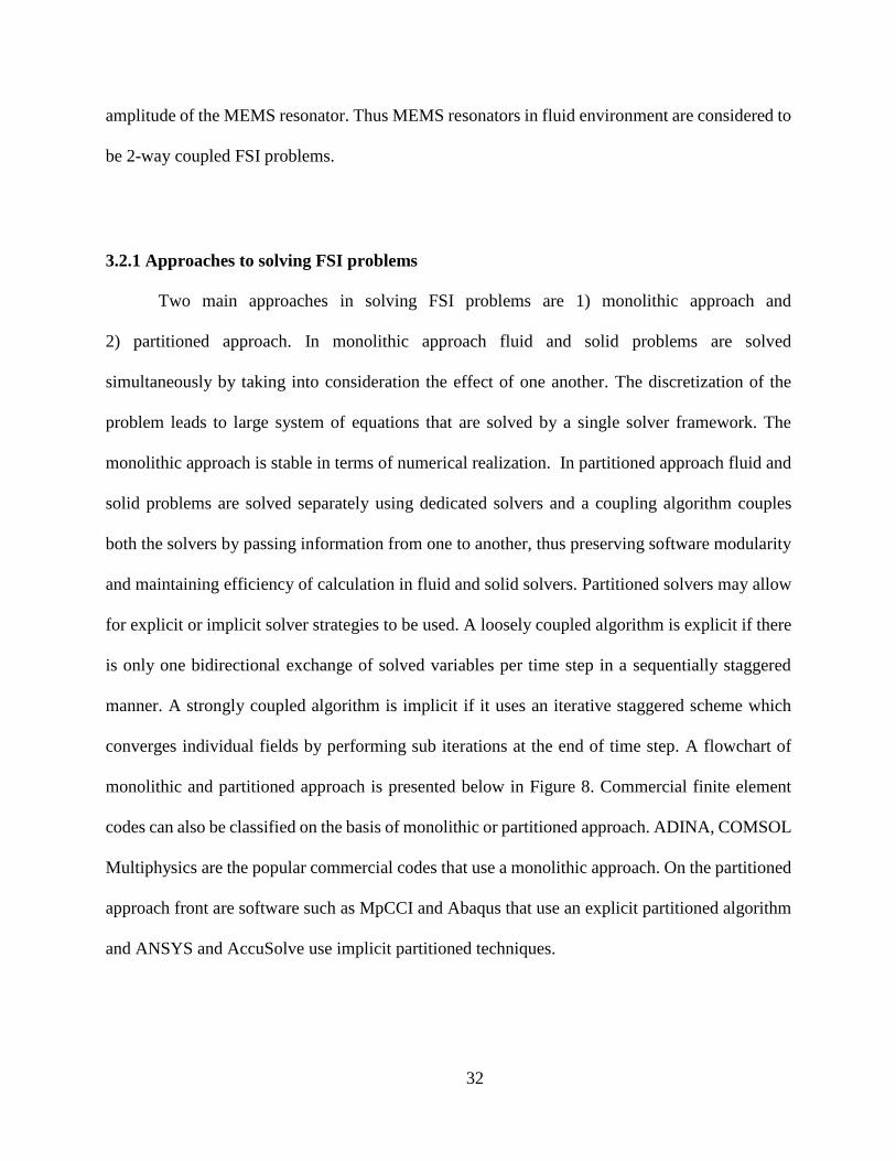
3.2.1 Approaches to solving FSI problems
Two main approaches in solving FSI problems are 1) monolithic approach and
2) partitioned approach. In monolithic approach fluid and solid problems are solved
simultaneously by taking into consideration the effect of one another. The discretization of the
problem leads to large system of equations that are solved by a single solver framework. The
monolithic approach is stable in terms of numerical realization. In partitioned approach fluid and
solid problems are solved separately using dedicated solvers and a coupling algorithm couples
both the solvers by passing information from one to another, thus preserving software modularity
and maintaining efficiency of calculation in fluid and solid solvers. Partitioned solvers may allow
for explicit or implicit solver strategies to be used. A loosely coupled algorithm is explicit if there
is only one bidirectional exchange of solved variables per time step in a sequentially staggered
manner. A strongly coupled algorithm is implicit if it uses an iterative staggered scheme which
converges individual fields by performing sub iterations at the end of time step. A flowchart of
monolithic and partitioned approach is presented below in Figure 8. Commercial finite element
codes can also be classified on the basis of monolithic or partitioned approach. ADINA, COMSOL
Multiphysics are the popular commercial codes that use a monolithic approach. On the partitioned
approach front are software such as MpCCI and Abaqus that use an explicit partitioned algorithm
and ANSYS and AccuSolve use implicit partitioned techniques.
33
Dimensionless numbers are used to quantify the extent of coupling between fluid and
structure phases [37]. Mass number Ma is defined as the ratio of density of the fluid to the density
of the structure i.e.,
𝑀𝑎 = 𝜌𝑓
𝜌𝑠 (3.1)
If Ma is close to 1, inertial effects of fluid are important and have to be taken into
consideration.
Cauchy number Cy is the ratio between the dynamic pressure and the elasticity of the
structure
𝐶𝑦 = 𝜌𝑓𝑉2
𝐸 (3.2)
Figure 8 -schematic showing monolithic and partitioned approaches
34
Cauchy number indicates the deformations induced by flow. If Cy is small, structure is rigid
and deformations induced by flow may not be significant. These numbers can give an idea about
the relative strength of each domain in governing the final outcome of the problem and hence serve
as a good starting point in the design process.
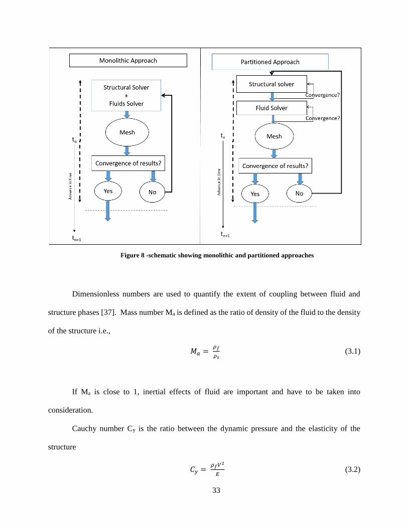
At the fluid-structure interface, the exchange of data is usually in the form of displacement
data from the structure is transferred to the fluid domain and force applied by the fluid on the
structure is passed as force data through fluid-structure interface. An overview of general methods
applied to study FSI problems is given below in Figure 9 [37]
(Reprinted from Fluid-Structure Interaction and uncertainties: Ansys and Fluent Tools, Abdelkhalak El Hami, Bouchaib Radi,.
With permission from John Wiley and Sons, copyright ISTE Ltd 2017)
Figure 9 – Overview of FSI methods
35
3.2.2 Structure coupled with stagnant fluid (frequency domain approach [37])
The state of the coupled systems is described by displacement in the structural domain and
pressure field in the fluid domain. The analysis framework is based on the vibrations in the
structure and the fluid. In linear problems without large deflections, vibrations of the structure are
defined in terms of frequency. The equilibrium equation of the solid can be written in Cartesian
coordinate system as:
𝜔2𝜌𝑠𝑢𝑖 + 𝜕𝜎𝑖𝑗(𝑢)
𝜕𝑥𝑗= 0 (3.3)
Without any external forces. The boundary conditions on the constrained boundary and stress-free
boundary are given by:
𝑢𝑖 = 0 𝑜𝑛 𝑐𝑜𝑛𝑠𝑡𝑟𝑎𝑖𝑛𝑒𝑑 𝑏𝑜𝑢𝑛𝑑𝑎𝑟𝑦 (3.4)
𝜎𝑖𝑗 (𝑢)𝑛𝑗𝑆 = 0 𝑜𝑛 𝑓𝑟𝑒𝑒 𝑏𝑜𝑢𝑛𝑑𝑎𝑟𝑦 (3.5)
Grouping together, an equation for displacement field can be deduced (Navier equation)
𝜌𝑠𝜔2𝑢𝑖 + (𝜆 + 𝜇)
𝜕
𝜕𝑥(
𝜕𝑢𝑗
𝜕𝑥𝑗) + 𝜇
𝜕2𝑢𝑖
𝜕𝑥𝑗𝜕𝑥𝑗= 0 (3.6)
Helmholtz equation describes the propagation of waves as a function of frequency
−𝜔2
𝑐2 𝑝 − 𝜕2𝑝
𝜕𝑥𝑖 𝜕𝑥𝑖 = 0 𝑖𝑛 𝑓𝑙𝑢𝑖𝑑 𝑑𝑜𝑚𝑎𝑖𝑛 (3.7)
With boundary conditions given as
𝜕𝑝
𝜕𝑥𝑗𝑛𝑗
𝐹 = 0 (3.8)
𝑝 = 0 (3.9)
The boundary condition prescribed by 3.8 models the presence of a fixed wall bounding
the fluid domain and boundary condition given by 3.9 models the acoustic free surface dictating
that pressure fluctuations are equal to zero.
36
In frequency domain analysis in Ansys workbench (Modal and Harmonic analysis), fluid-structure
interaction is considered in the finite element matrix as [45]
[𝑀𝑠 0
𝜌𝑅𝑇 𝑀𝑓] {�̈�
�̈�} + [
𝐾𝑠 −𝑅0 𝐾𝑓
] {𝑈𝐹} = {
𝐹𝑠
𝐹𝑓} (3.11)
where ρ denotes fluid density, R is the coupling matrix associated with nodes involved in fluid-
structure interface. The subscripts ‘s’ and ‘f ’ indicate solid and fluid fields.
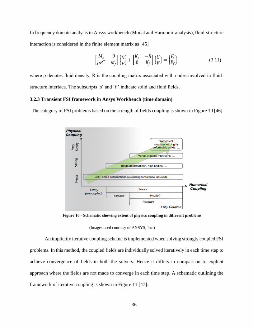
3.2.3 Transient FSI framework in Ansys Workbench (time domain)
The category of FSI problems based on the strength of fields coupling is shown in Figure 10 [46].
(Images used courtesy of ANSYS, Inc.)
An implicitly iterative coupling scheme is implemented when solving strongly coupled FSI
problems. In this method, the coupled fields are individually solved iteratively in each time step to
achieve convergence of fields in both the solvers. Hence it differs in comparison to explicit
approach where the fields are not made to converge in each time step. A schematic outlining the
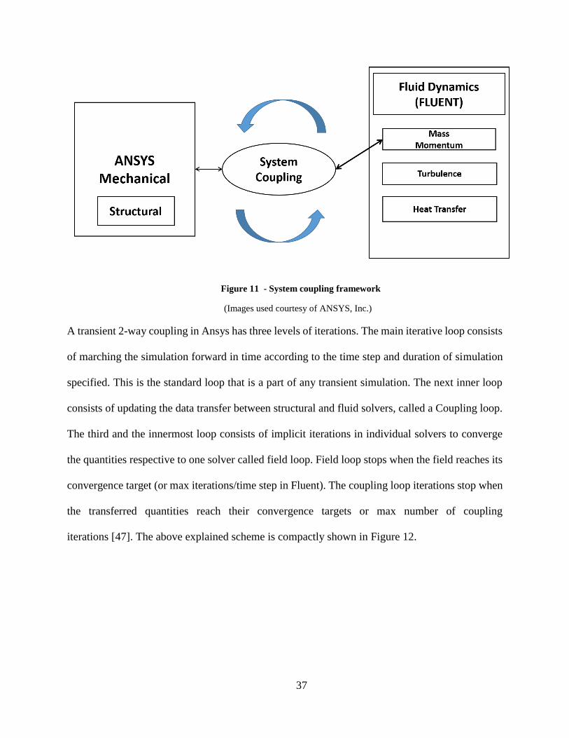
framework of iterative coupling is shown in Figure 11 [47].
Figure 10 - Schematic showing extent of physics coupling in different problems
37
(Images used courtesy of ANSYS, Inc.)
A transient 2-way coupling in Ansys has three levels of iterations. The main iterative loop consists
of marching the simulation forward in time according to the time step and duration of simulation
specified. This is the standard loop that is a part of any transient simulation. The next inner loop
consists of updating the data transfer between structural and fluid solvers, called a Coupling loop.
The third and the innermost loop consists of implicit iterations in individual solvers to converge
the quantities respective to one solver called field loop. Field loop stops when the field reaches its
convergence target (or max iterations/time step in Fluent). The coupling loop iterations stop when
the transferred quantities reach their convergence targets or max number of coupling
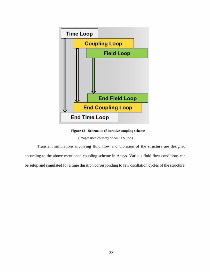
iterations [47]. The above explained scheme is compactly shown in Figure 12.
Figure 11 - System coupling framework
38
(Images used courtesy of ANSYS, Inc.)
Transient simulations involving fluid flow and vibration of the structure are designed
according to the above mentioned coupling scheme in Ansys. Various fluid flow conditions can
be setup and simulated for a time duration corresponding to few oscillation cycles of the structure.
Figure 12 - Schematic of iterative coupling scheme
39
Chapter 4
4.1 Setup of computational model in ANSYS Workbench
Ansys workbench is the project management suite which contains all kind of physics
capabilities as modules, easy to integrate project workflow and has in-built post processing
capabilities which make the process of implementing Finite Element methods quicker and easier.
All the computational analyses presented in this thesis have been carried out in the workbench
interface. The overall workflow of the analyses carried out are briefly described below and
elaborately explained in their respective sections.
First set of analyses concentrating on the frequency domain have been carried out using
Modal, Harmonic response, Transient structural modules with ACT Piezo & MEMS and ACT
Acoustics extensions available in Workbench [45, 48]. The first step towards understanding the
basics of frequency response of a resonator device is eigenfrequency analyses to extract the natural
frequencies of the structure and corresponding mode shapes. This analysis is carried out first in
vacuum, then in liquids of different kinematic viscosities to understand the damping mechanisms
associated with different fluids, and to gauge the shift in the natural frequencies under different
fluid environments. Second step is to apply a particular periodic load on the resonator and extract
the frequency response of the resonator within a range of frequencies, thus understanding the
operating characteristics of the sensor. Again, harmonic response is gauged in different fluid
environments. In order to understand the binding events happening at the sensor surface, point
masses of different magnitudes are attached to the surface of the biosensor at different positions
and the change in the natural frequency and harmonic response of the sensor is observed, thus
providing an estimate about the mass sensitivity of the biosensor.
40
In order to understand the characteristics of the biosensor with respect to time, time domain
analysis has been carried out using the Transient Structural, Fluid flow (FLUENT) and system
coupling modules, thus incorporating computational fluid dynamics. Transient analysis has also
been carried out with different fluids to understand the dynamic behavior in respective fluid
environments. Mesh and field quantities have been converged. The analysis is benchmarked
against experimental data from AFM for a model system and also compared against analytical
values.
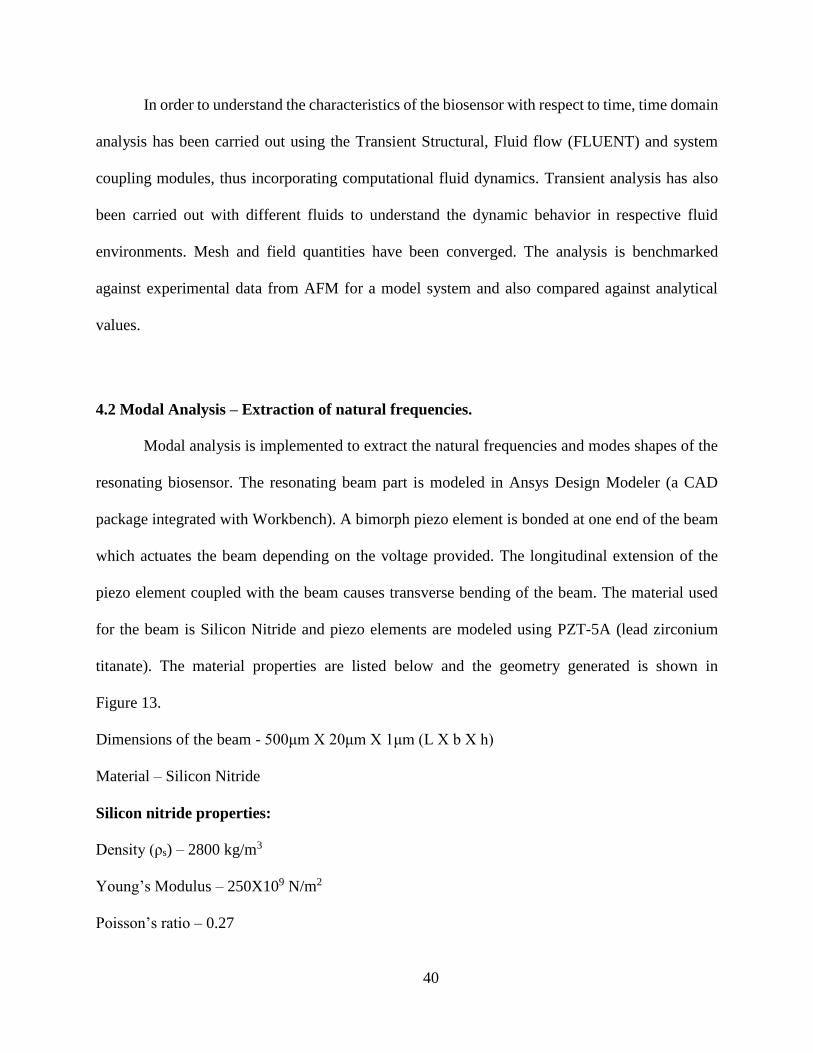
4.2 Modal Analysis – Extraction of natural frequencies.
Modal analysis is implemented to extract the natural frequencies and modes shapes of the
resonating biosensor. The resonating beam part is modeled in Ansys Design Modeler (a CAD
package integrated with Workbench). A bimorph piezo element is bonded at one end of the beam
which actuates the beam depending on the voltage provided. The longitudinal extension of the
piezo element coupled with the beam causes transverse bending of the beam. The material used
for the beam is Silicon Nitride and piezo elements are modeled using PZT-5A (lead zirconium
titanate). The material properties are listed below and the geometry generated is shown in
Figure 13.
Dimensions of the beam - 500μm X 20μm X 1μm (L X b X h)
Material – Silicon Nitride
Silicon nitride properties:
Density (ρs) – 2800 kg/m3
Young’s Modulus – 250X109 N/m2
Poisson’s ratio – 0.27
41
Bimorph Piezo dimensions - 100μm X 20μm X 2μm
Material - PZT 5A
PZT material properties:
Density – 7500 kg/m3
Anisotropic Elasticity Matrix (Pa):
[ 1.32𝐸 + 11 7.3𝐸 + 10 7.1𝐸 + 10 0 0 07.3𝐸 + 10 1.15𝐸 + 11 7.3𝐸 + 10 0 0 07.1𝐸 + 10 7.3𝐸 + 10 1.32𝐸 + 11 0 0 0
0 0 0 2.6𝐸 + 10 0 00 0 0 0 2.6𝐸 + 10 00 0 0 0 0 3𝐸 + 10]
Polarization axis – along Y
Piezoelectric coefficients: e31 = -4.1 As/m2, e33 = 14.1 As/m2, e15 = 10.5 As/m2
Permittivity constants: ep11 = 804, ep33 = 660;
Figure 13 - Schematic of beam and bimorph piezo strip
42
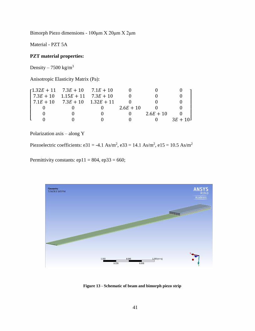
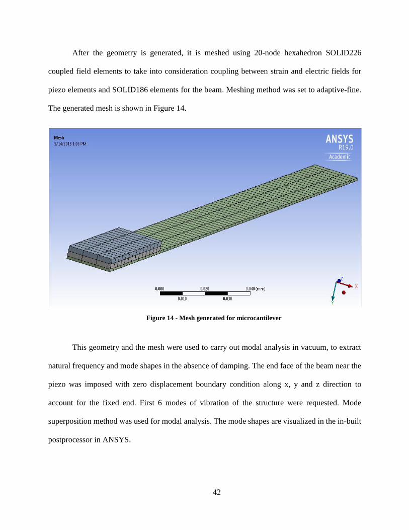
After the geometry is generated, it is meshed using 20-node hexahedron SOLID226
coupled field elements to take into consideration coupling between strain and electric fields for
piezo elements and SOLID186 elements for the beam. Meshing method was set to adaptive-fine.
The generated mesh is shown in Figure 14.
This geometry and the mesh were used to carry out modal analysis in vacuum, to extract
natural frequency and mode shapes in the absence of damping. The end face of the beam near the
piezo was imposed with zero displacement boundary condition along x, y and z direction to
account for the fixed end. First 6 modes of vibration of the structure were requested. Mode
superposition method was used for modal analysis. The mode shapes are visualized in the in-built
postprocessor in ANSYS.
Figure 14 - Mesh generated for microcantilever
43
4.3 Harmonic Response Analysis
In order to check the frequency response of the structure under a specific piezoelectric
supply voltage, harmonic response analysis was carried out. In order to save computation time,
only first mode of vibration is considered. Depending upon the frequencies obtained by modal
analysis, the range of frequencies to sweep were restricted to 1000Hz to 10,000Hz, with a solution
interval of 100 points to check for response near the first vibration mode. Solution method was set
to Full. Structural damping was ignored. Same displacement boundary condition was applied as in
modal analysis. Voltage boundary conditions and loads were setup in order to produce transverse
bending in the beam. The surface of the piezo in contact with the beam was assigned zero voltage
(grounded) and the top piezo surface was assigned a voltage of 5V. This voltage is applied at each
of the frequencies requested in the range. Voltage coupling condition was assigned to the boundary
between the two piezo strips. Frequency response for the range of sweep frequencies and total
deformation of the beam were the results requested in the analysis.
4.4 Frequency domain analysis in fluid environment
In order to characterize the frequency domain behavior of the piezo actuated beam in fluid
environment, fluid-structure interaction coupled vibroacoustics analysis was carried out. The
cantilever beam geometry was modeled with an enclosure containing fluid. The enclosure was
defined as acoustic body with incompressible fluid. As described in section 4.2 and 4.3, modal and
harmonic response analysis was carried out for the beam structure immersed in a stagnant fluid.
Using the Enclosure feature in Design Modeler, two interconnected cavities containing fluid were
defined. The enclosure immediately in contact with the beam structure was defined as nearfield
and the enclosure in contact with nearfield was defined as farfield. Nearfield enclosure body has a
finer mesh to capture the deformation of the beam and finely resolve pressure fluctuations around
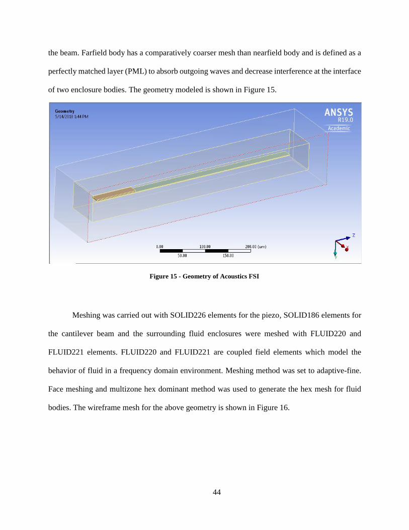
44
the beam. Farfield body has a comparatively coarser mesh than nearfield body and is defined as a
perfectly matched layer (PML) to absorb outgoing waves and decrease interference at the interface
of two enclosure bodies. The geometry modeled is shown in Figure 15.
Meshing was carried out with SOLID226 elements for the piezo, SOLID186 elements for
the cantilever beam and the surrounding fluid enclosures were meshed with FLUID220 and
FLUID221 elements. FLUID220 and FLUID221 are coupled field elements which model the
behavior of fluid in a frequency domain environment. Meshing method was set to adaptive-fine.
Face meshing and multizone hex dominant method was used to generate the hex mesh for fluid
bodies. The wireframe mesh for the above geometry is shown in Figure 16.
Figure 15 - Geometry of Acoustics FSI
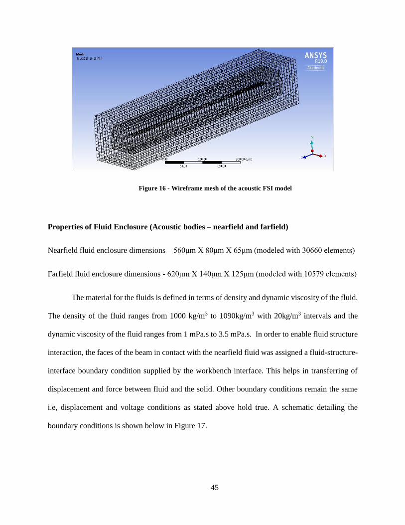
45
Properties of Fluid Enclosure (Acoustic bodies – nearfield and farfield)
Nearfield fluid enclosure dimensions – 560μm X 80μm X 65μm (modeled with 30660 elements)
Farfield fluid enclosure dimensions - 620μm X 140μm X 125μm (modeled with 10579 elements)
The material for the fluids is defined in terms of density and dynamic viscosity of the fluid.
The density of the fluid ranges from 1000 kg/m3 to 1090kg/m3 with 20kg/m3 intervals and the
dynamic viscosity of the fluid ranges from 1 mPa.s to 3.5 mPa.s. In order to enable fluid structure
interaction, the faces of the beam in contact with the nearfield fluid was assigned a fluid-structure-
interface boundary condition supplied by the workbench interface. This helps in transferring of
displacement and force between fluid and the solid. Other boundary conditions remain the same
i.e, displacement and voltage conditions as stated above hold true. A schematic detailing the
boundary conditions is shown below in Figure 17.
Figure 16 - Wireframe mesh of the acoustic FSI model
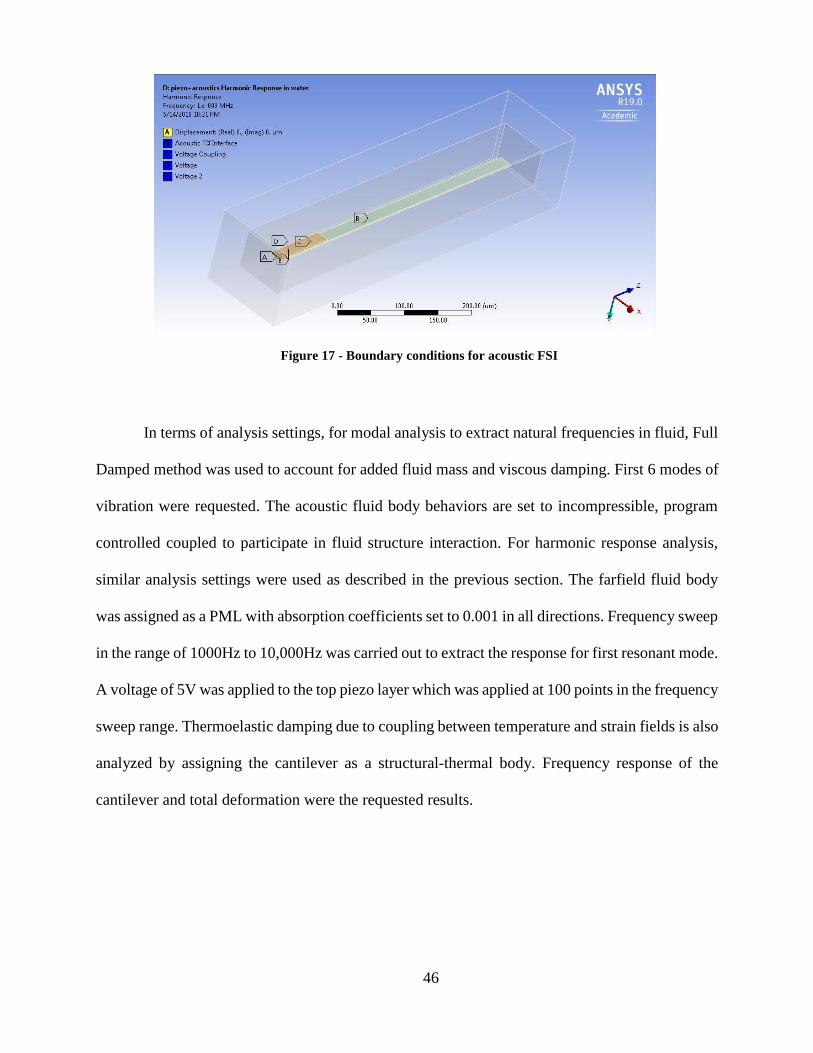
46
In terms of analysis settings, for modal analysis to extract natural frequencies in fluid, Full
Damped method was used to account for added fluid mass and viscous damping. First 6 modes of
vibration were requested. The acoustic fluid body behaviors are set to incompressible, program
controlled coupled to participate in fluid structure interaction. For harmonic response analysis,
similar analysis settings were used as described in the previous section. The farfield fluid body
was assigned as a PML with absorption coefficients set to 0.001 in all directions. Frequency sweep
in the range of 1000Hz to 10,000Hz was carried out to extract the response for first resonant mode.
A voltage of 5V was applied to the top piezo layer which was applied at 100 points in the frequency
sweep range. Thermoelastic damping due to coupling between temperature and strain fields is also
analyzed by assigning the cantilever as a structural-thermal body. Frequency response of the
cantilever and total deformation were the requested results.
Figure 17 - Boundary conditions for acoustic FSI
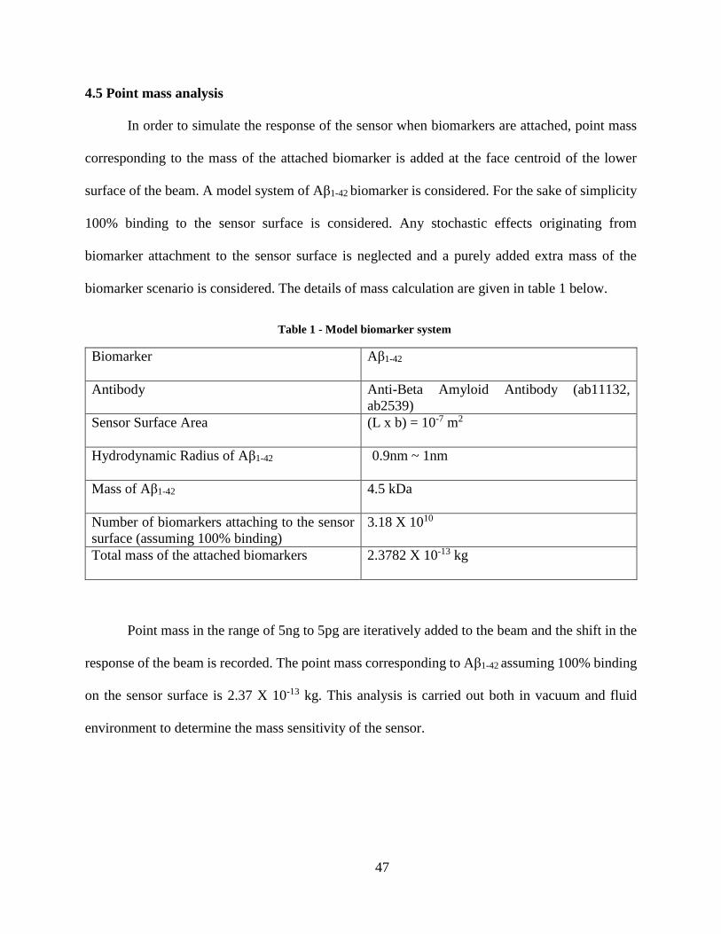
47
4.5 Point mass analysis
In order to simulate the response of the sensor when biomarkers are attached, point mass
corresponding to the mass of the attached biomarker is added at the face centroid of the lower
surface of the beam. A model system of Aβ1-42 biomarker is considered. For the sake of simplicity
100% binding to the sensor surface is considered. Any stochastic effects originating from
biomarker attachment to the sensor surface is neglected and a purely added extra mass of the
biomarker scenario is considered. The details of mass calculation are given in table 1 below.
Table 1 - Model biomarker system
Biomarker Aβ1-42
Antibody Anti-Beta Amyloid Antibody (ab11132,
ab2539)
Sensor Surface Area (L x b) = 10-7 m2
Hydrodynamic Radius of Aβ1-42 0.9nm ~ 1nm
Mass of Aβ1-42 4.5 kDa
Number of biomarkers attaching to the sensor
surface (assuming 100% binding)
3.18 X 10¹⁰
Total mass of the attached biomarkers 2.3782 X 10⁻¹³ kg
Point mass in the range of 5ng to 5pg are iteratively added to the beam and the shift in the
response of the beam is recorded. The point mass corresponding to Aβ1-42 assuming 100% binding
on the sensor surface is 2.37 X 10⁻¹³ kg. This analysis is carried out both in vacuum and fluid
environment to determine the mass sensitivity of the sensor.
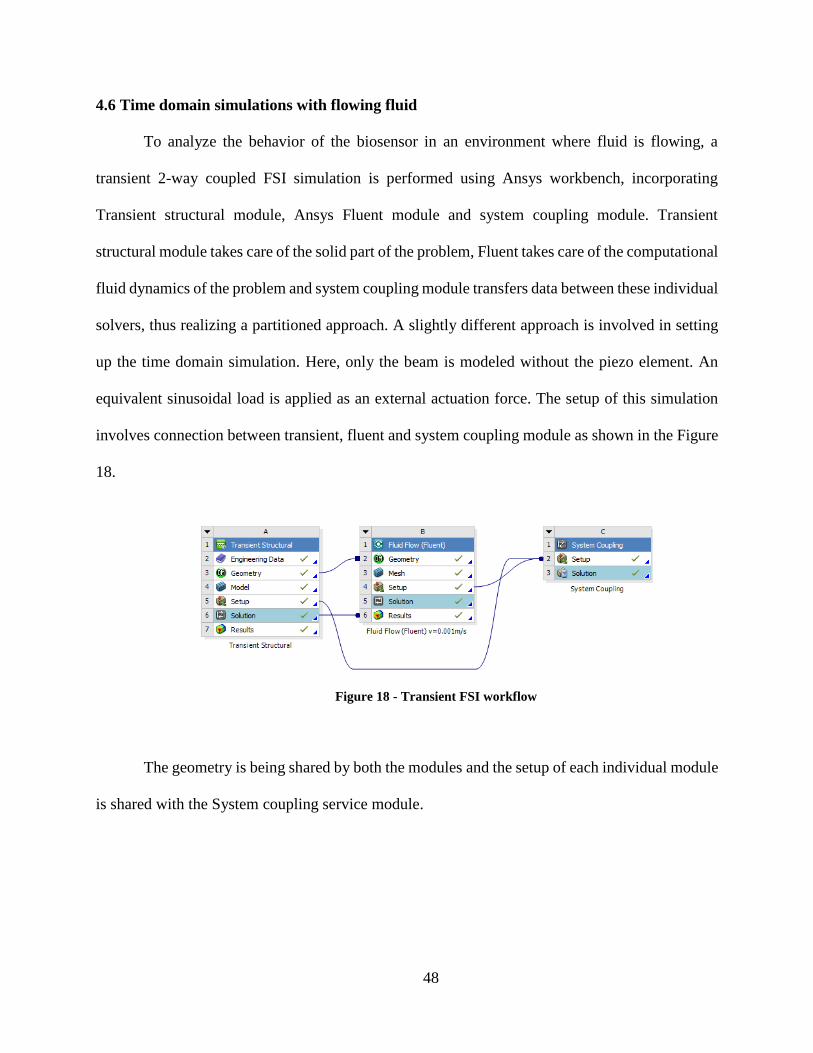
48
4.6 Time domain simulations with flowing fluid
To analyze the behavior of the biosensor in an environment where fluid is flowing, a
transient 2-way coupled FSI simulation is performed using Ansys workbench, incorporating
Transient structural module, Ansys Fluent module and system coupling module. Transient
structural module takes care of the solid part of the problem, Fluent takes care of the computational
fluid dynamics of the problem and system coupling module transfers data between these individual
solvers, thus realizing a partitioned approach. A slightly different approach is involved in setting
up the time domain simulation. Here, only the beam is modeled without the piezo element. An
equivalent sinusoidal load is applied as an external actuation force. The setup of this simulation
involves connection between transient, fluent and system coupling module as shown in the Figure
18.
The geometry is being shared by both the modules and the setup of each individual module
is shared with the System coupling service module.
Figure 18 - Transient FSI workflow
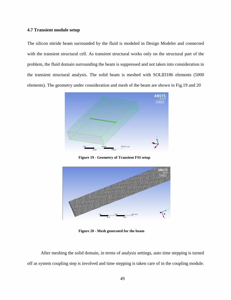
49
4.7 Transient module setup
The silicon nitride beam surrounded by the fluid is modeled in Design Modeler and connected
with the transient structural cell. As transient structural works only on the structural part of the
problem, the fluid domain surrounding the beam is suppressed and not taken into consideration in
the transient structural analysis. The solid beam is meshed with SOLID186 elements (5000
elements). The geometry under consideration and mesh of the beam are shown in Fig.19 and 20
After meshing the solid domain, in terms of analysis settings, auto time stepping is turned
off as system coupling step is involved and time stepping is taken care of in the coupling module.
Figure 19 - Geometry of Transient FSI setup
Figure 20 - Mesh generated for the beam
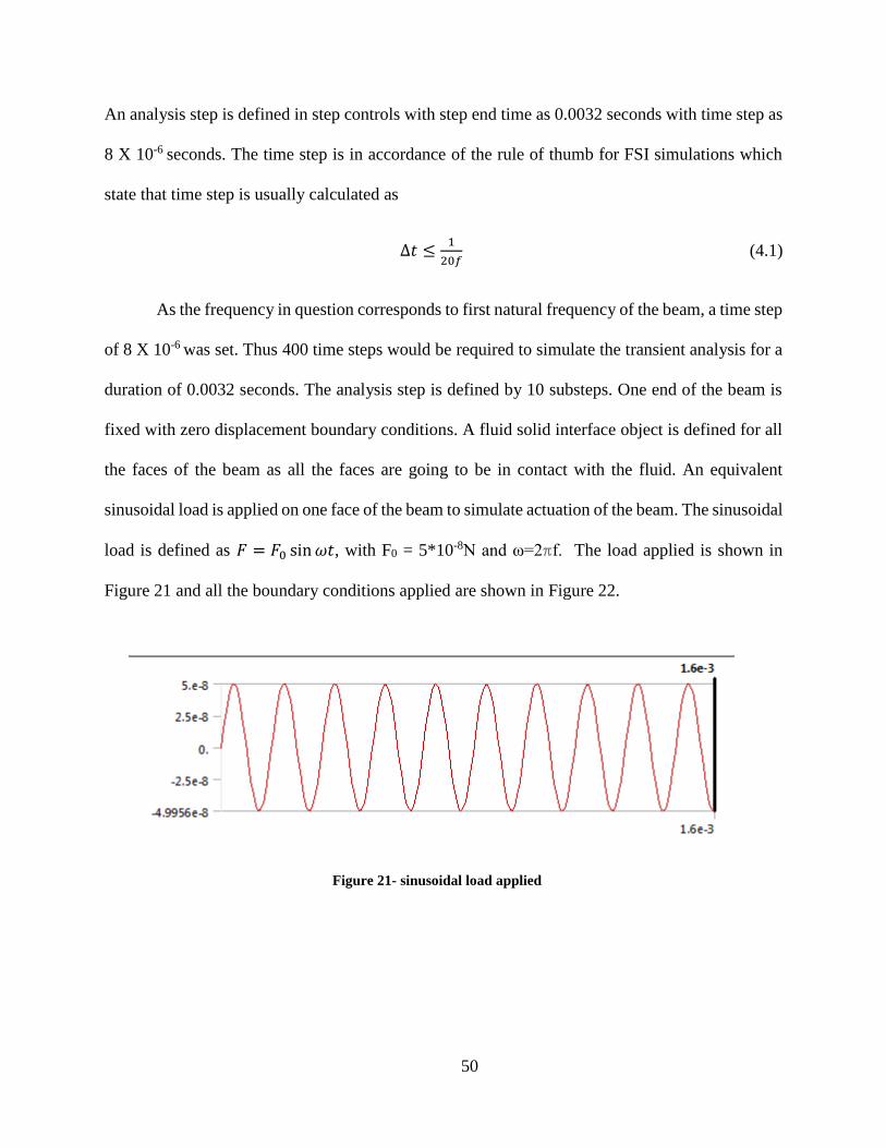
50
An analysis step is defined in step controls with step end time as 0.0032 seconds with time step as
8 X 10⁻⁶ seconds. The time step is in accordance of the rule of thumb for FSI simulations which
state that time step is usually calculated as
∆𝑡 ≤1
20𝑓 (4.1)
As the frequency in question corresponds to first natural frequency of the beam, a time step
of 8 X 10⁻⁶ was set. Thus 400 time steps would be required to simulate the transient analysis for a
duration of 0.0032 seconds. The analysis step is defined by 10 substeps. One end of the beam is
fixed with zero displacement boundary conditions. A fluid solid interface object is defined for all
the faces of the beam as all the faces are going to be in contact with the fluid. An equivalent
sinusoidal load is applied on one face of the beam to simulate actuation of the beam. The sinusoidal
load is defined as 𝐹 = 𝐹0 sin𝜔𝑡, with F0 = 5*10-8N and ω=2ℼf. The load applied is shown in
Figure 21 and all the boundary conditions applied are shown in Figure 22.
Fig.16 Figure 21- sinusoidal load applied
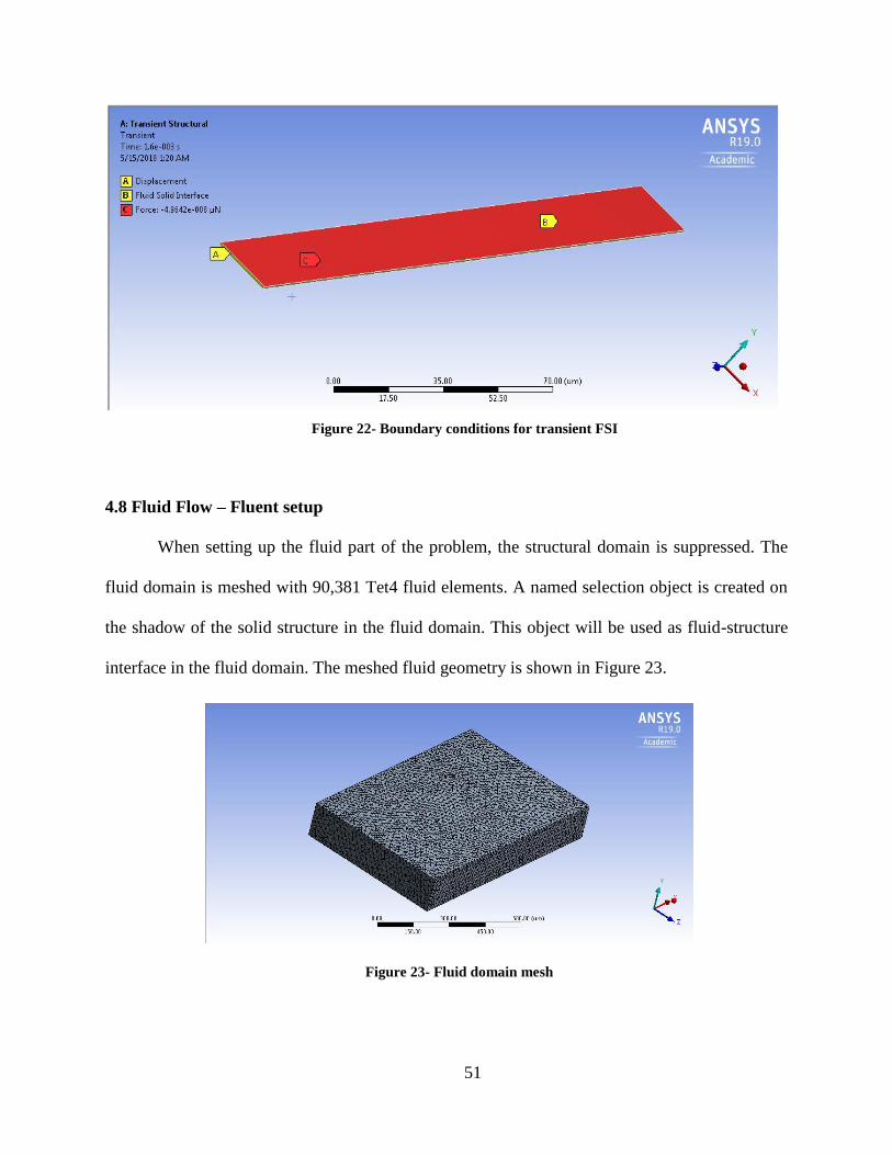
51
4.8 Fluid Flow – Fluent setup
When setting up the fluid part of the problem, the structural domain is suppressed. The
fluid domain is meshed with 90,381 Tet4 fluid elements. A named selection object is created on
the shadow of the solid structure in the fluid domain. This object will be used as fluid-structure
interface in the fluid domain. The meshed fluid geometry is shown in Figure 23.
Figure 22- Boundary conditions for transient FSI
Figure 23- Fluid domain mesh
52
The next steps of the setup are performed in Fluent CFD module. Double precision, 3D,
serial Fluent solver is selected to perform computational fluid dynamics part of the problem.
Transient simulation is selected and the fluid model selected is viscous laminar. Water is selected
as the fluid medium. Fluent has a database of materials with properties already loaded. The fluid
material with desired properties is added and the fluid cell zones are assigned that particular fluid.
In order to take into account the deformation of the fluid-structure-interface, dynamic mesh is
implemented in Fluent. The dynamic mesh model in Ansys Fluent can be used to model flows
where the shape of the domain is changing with time due to motion on the domain boundaries.
When the model contains moving and non-moving regions, these regions need to be identified and
assigned appropriate deformation behavior. In this case, the fluid-solid-interface is assigned
system coupling dynamic mesh zone, the interior of the fluid is assigned as deforming mesh zone.
Smoothing mesh method is applied with diffusion parameter set to 2, diffusion function set to
boundary-distance.
In order to achieve better convergence with the results, an absolute residual criteria of
10-4 is imposed on continuity and x, y & z velocities. In terms of analysis settings, pressure-velocity
coupling is used with a coupled scheme. Spatial discretization wise, gradient method is set to Least
Squares Cell Based technique, pressure is set to second order and momentum is set to second order
upwind. Transient formulation is set to first order implicit. In terms of solution controls, explicit
relaxation factors for momentum and pressure are set to 0.75 each and under-relaxation factors for
density and body forces are set to 1. Standard initialization scheme is used to initialize the flow
field. After flow initialization, the calculations are run through the system coupling module.
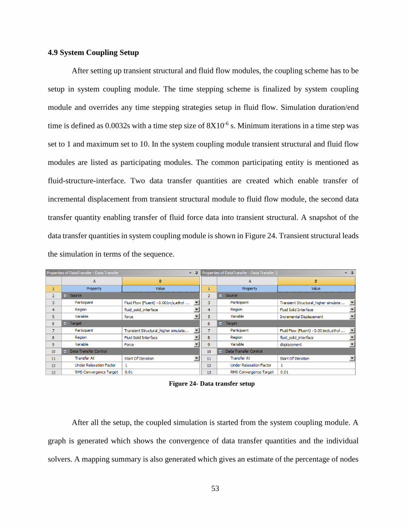
53
4.9 System Coupling Setup
After setting up transient structural and fluid flow modules, the coupling scheme has to be
setup in system coupling module. The time stepping scheme is finalized by system coupling
module and overrides any time stepping strategies setup in fluid flow. Simulation duration/end
time is defined as 0.0032s with a time step size of 8X10⁻⁶ s. Minimum iterations in a time step was
set to 1 and maximum set to 10. In the system coupling module transient structural and fluid flow
modules are listed as participating modules. The common participating entity is mentioned as
fluid-structure-interface. Two data transfer quantities are created which enable transfer of
incremental displacement from transient structural module to fluid flow module, the second data
transfer quantity enabling transfer of fluid force data into transient structural. A snapshot of the
data transfer quantities in system coupling module is shown in Figure 24. Transient structural leads
the simulation in terms of the sequence.
After all the setup, the coupled simulation is started from the system coupling module. A
graph is generated which shows the convergence of data transfer quantities and the individual
solvers. A mapping summary is also generated which gives an estimate of the percentage of nodes
Figure 24- Data transfer setup
54
mapped from source to target region. After the simulation has completed, CFD-post, a post
processing module provided by Ansys Workbench is used to post process the results. Pressure and
velocity quantities near the cantilever are analyzed. Drag force imposed on the fluid-structure
interface normal to the direction of vibration of the cantilever is monitored for the full simulation
duration. Net forces due to pressure and viscous effects at the fluid-structure interface are also
monitored for three different fluids namely acetone (ρ=791kg/m3, μ=0.000331 kg/m-s), water
(ρ=998.2kg/m3, μ=0.001003 kg/m-s) and ethylene glycol (ρ=1111.4kg/m3, μ=0.0157 kg/m-s). 3D
vector graphics are used to visualize the flow field near the cantilever. Contour plots are generated
at various planes in the flow domain to visualize pressure and velocity distributions. Animations
of the time steps are generated to visualize the dynamic event of cantilever vibrating in a fluid
environment.
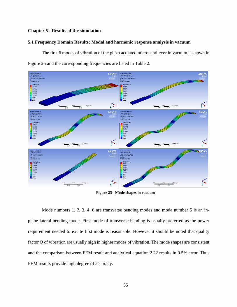
55
Chapter 5 - Results of the simulation
5.1 Frequency Domain Results: Modal and harmonic response analysis in vacuum
The first 6 modes of vibration of the piezo actuated microcantilever in vacuum is shown in
Figure 25 and the corresponding frequencies are listed in Table 2.
Mode numbers 1, 2, 3, 4, 6 are transverse bending modes and mode number 5 is an in-
plane lateral bending mode. First mode of transverse bending is usually preferred as the power
requirement needed to excite first mode is reasonable. However it should be noted that quality
factor Q of vibration are usually high in higher modes of vibration. The mode shapes are consistent
and the comparison between FEM result and analytical equation 2.22 results in 0.5% error. Thus
FEM results provide high degree of accuracy.
Figure 25 - Mode shapes in vacuum
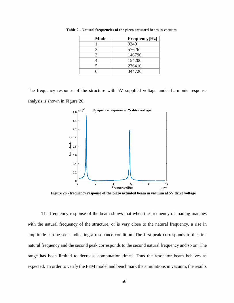
56
Table 2 - Natural frequencies of the piezo actuated beam in vacuum
Mode Frequency[Hz]
1 9349
2 57626
3 146790
4 154200
5 236410
6 344720
The frequency response of the structure with 5V supplied voltage under harmonic response
analysis is shown in Figure 26.
The frequency response of the beam shows that when the frequency of loading matches
with the natural frequency of the structure, or is very close to the natural frequency, a rise in
amplitude can be seen indicating a resonance condition. The first peak corresponds to the first
natural frequency and the second peak corresponds to the second natural frequency and so on. The
range has been limited to decrease computation times. Thus the resonator beam behaves as
expected. In order to verify the FEM model and benchmark the simulations in vacuum, the results
Figure 26 - frequency response of the piezo actuated beam in vacuum at 5V drive voltage
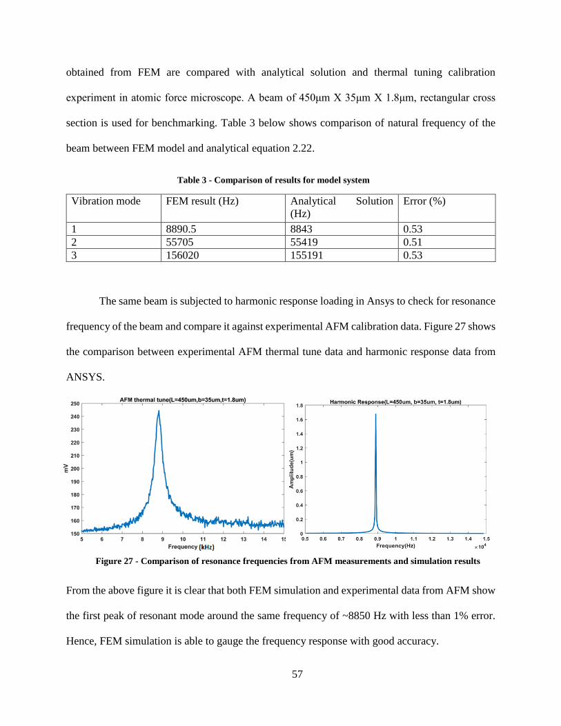
57
obtained from FEM are compared with analytical solution and thermal tuning calibration
experiment in atomic force microscope. A beam of 450μm X 35μm X 1.8μm, rectangular cross
section is used for benchmarking. Table 3 below shows comparison of natural frequency of the
beam between FEM model and analytical equation 2.22.
Table 3 - Comparison of results for model system
Vibration mode FEM result (Hz) Analytical Solution
(Hz)
Error (%)
1 8890.5 8843 0.53
2 55705 55419 0.51
3 156020 155191 0.53
The same beam is subjected to harmonic response loading in Ansys to check for resonance
frequency of the beam and compare it against experimental AFM calibration data. Figure 27 shows
the comparison between experimental AFM thermal tune data and harmonic response data from
ANSYS.
Figure 27 - Comparison of resonance frequencies from AFM measurements and simulation results
From the above figure it is clear that both FEM simulation and experimental data from AFM show
the first peak of resonant mode around the same frequency of ~8850 Hz with less than 1% error.
Hence, FEM simulation is able to gauge the frequency response with good accuracy.
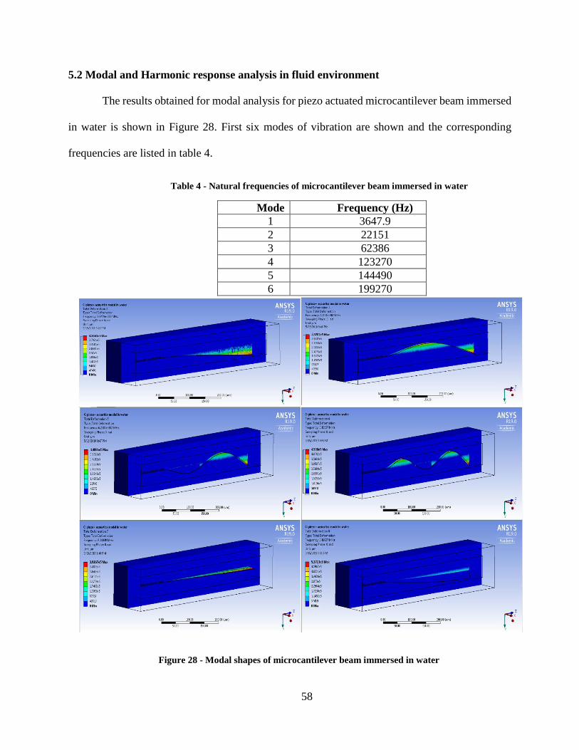
58
5.2 Modal and Harmonic response analysis in fluid environment
The results obtained for modal analysis for piezo actuated microcantilever beam immersed
in water is shown in Figure 28. First six modes of vibration are shown and the corresponding
frequencies are listed in table 4.
Table 4 - Natural frequencies of microcantilever beam immersed in water
Mode Frequency (Hz)
1 3647.9
2 22151
3 62386
4 123270
5 144490
6 199270
Figure 28 - Modal shapes of microcantilever beam immersed in water
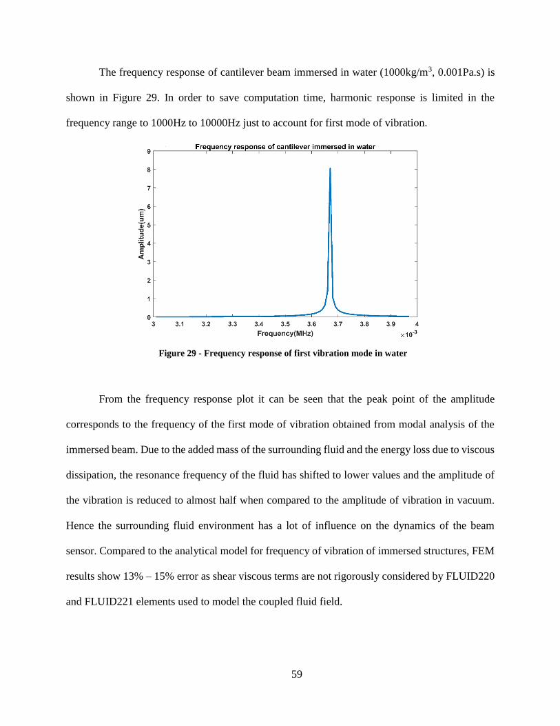
59
The frequency response of cantilever beam immersed in water (1000kg/m3, 0.001Pa.s) is
shown in Figure 29. In order to save computation time, harmonic response is limited in the
frequency range to 1000Hz to 10000Hz just to account for first mode of vibration.
From the frequency response plot it can be seen that the peak point of the amplitude
corresponds to the frequency of the first mode of vibration obtained from modal analysis of the
immersed beam. Due to the added mass of the surrounding fluid and the energy loss due to viscous
dissipation, the resonance frequency of the fluid has shifted to lower values and the amplitude of
the vibration is reduced to almost half when compared to the amplitude of vibration in vacuum.
Hence the surrounding fluid environment has a lot of influence on the dynamics of the beam
sensor. Compared to the analytical model for frequency of vibration of immersed structures, FEM
results show 13% – 15% error as shear viscous terms are not rigorously considered by FLUID220
and FLUID221 elements used to model the coupled fluid field.
Figure 29 - Frequency response of first vibration mode in water
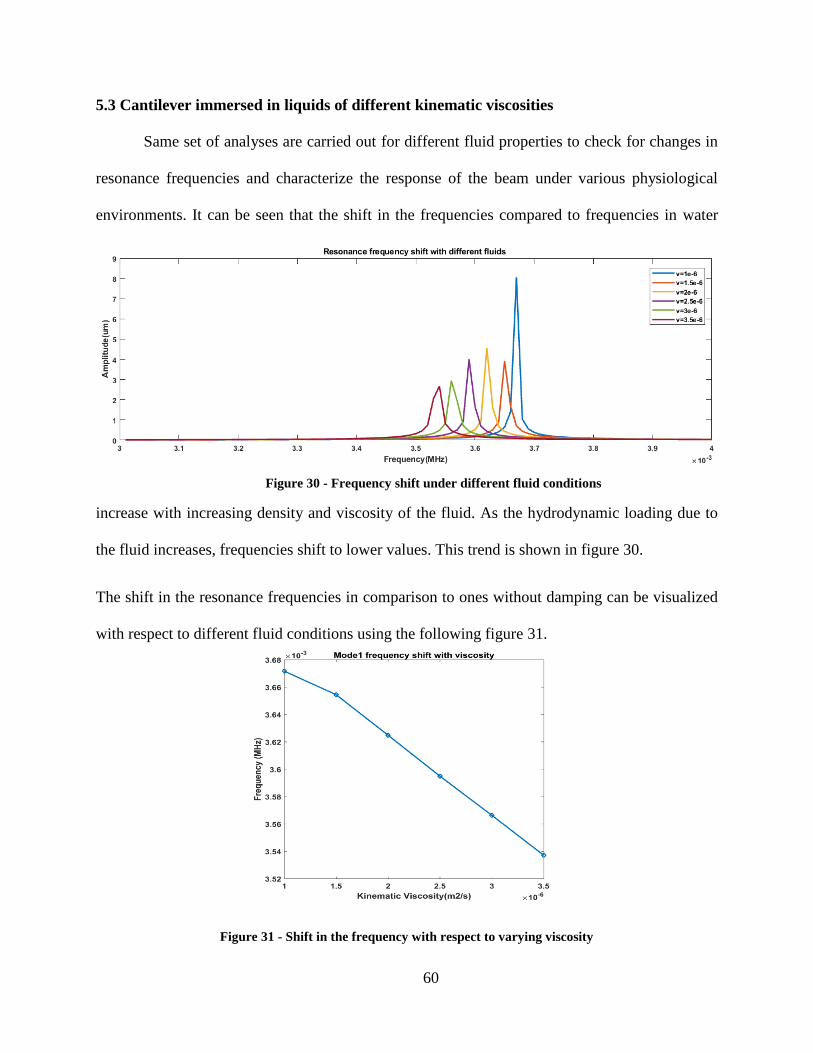
60
5.3 Cantilever immersed in liquids of different kinematic viscosities
Same set of analyses are carried out for different fluid properties to check for changes in
resonance frequencies and characterize the response of the beam under various physiological
environments. It can be seen that the shift in the frequencies compared to frequencies in water
increase with increasing density and viscosity of the fluid. As the hydrodynamic loading due to
the fluid increases, frequencies shift to lower values. This trend is shown in figure 30.
The shift in the resonance frequencies in comparison to ones without damping can be visualized
with respect to different fluid conditions using the following figure 31.
Figure 30 - Frequency shift under different fluid conditions
Figure 31 - Shift in the frequency with respect to varying viscosity
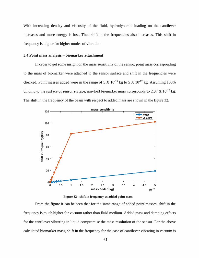
61
With increasing density and viscosity of the fluid, hydrodynamic loading on the cantilever
increases and more energy is lost. Thus shift in the frequencies also increases. This shift in
frequency is higher for higher modes of vibration.
5.4 Point mass analysis – biomarker attachment
In order to get some insight on the mass sensitivity of the sensor, point mass corresponding
to the mass of biomarker were attached to the sensor surface and shift in the frequencies were
checked. Point masses added were in the range of 5 X 10-15 kg to 5 X 10-12 kg. Assuming 100%
binding to the surface of sensor surface, amyloid biomarker mass corresponds to 2.37 X 10⁻¹³ kg.
The shift in the frequency of the beam with respect to added mass are shown in the figure 32.
From the figure it can be seen that for the same range of added point masses, shift in the
frequency is much higher for vacuum rather than fluid medium. Added mass and damping effects
for the cantilever vibrating in liquid compromise the mass resolution of the sensor. For the above
calculated biomarker mass, shift in the frequency for the case of cantilever vibrating in vacuum is
Figure 32 - shift in frequency vs added point mass
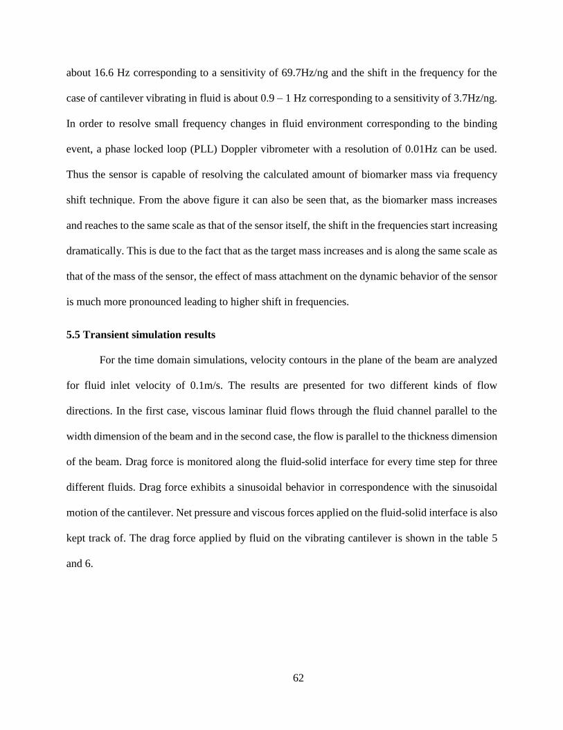
62
about 16.6 Hz corresponding to a sensitivity of 69.7Hz/ng and the shift in the frequency for the
case of cantilever vibrating in fluid is about 0.9 – 1 Hz corresponding to a sensitivity of 3.7Hz/ng.
In order to resolve small frequency changes in fluid environment corresponding to the binding
event, a phase locked loop (PLL) Doppler vibrometer with a resolution of 0.01Hz can be used.
Thus the sensor is capable of resolving the calculated amount of biomarker mass via frequency
shift technique. From the above figure it can also be seen that, as the biomarker mass increases
and reaches to the same scale as that of the sensor itself, the shift in the frequencies start increasing
dramatically. This is due to the fact that as the target mass increases and is along the same scale as
that of the mass of the sensor, the effect of mass attachment on the dynamic behavior of the sensor
is much more pronounced leading to higher shift in frequencies.
5.5 Transient simulation results
For the time domain simulations, velocity contours in the plane of the beam are analyzed
for fluid inlet velocity of 0.1m/s. The results are presented for two different kinds of flow
directions. In the first case, viscous laminar fluid flows through the fluid channel parallel to the
width dimension of the beam and in the second case, the flow is parallel to the thickness dimension
of the beam. Drag force is monitored along the fluid-solid interface for every time step for three
different fluids. Drag force exhibits a sinusoidal behavior in correspondence with the sinusoidal
motion of the cantilever. Net pressure and viscous forces applied on the fluid-solid interface is also
kept track of. The drag force applied by fluid on the vibrating cantilever is shown in the table 5
and 6.
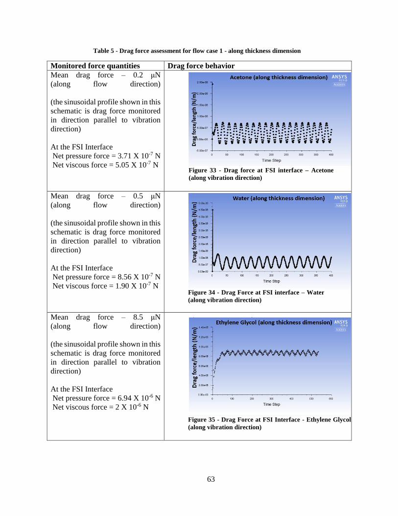
63
Table 5 - Drag force assessment for flow case 1 - along thickness dimension
Monitored force quantities Drag force behavior
Mean drag force – 0.2 μN
(along flow direction)
(the sinusoidal profile shown in this
schematic is drag force monitored
in direction parallel to vibration
direction)
At the FSI Interface
Net pressure force = 3.71 X 10⁻⁷ N
Net viscous force = 5.05 X 10⁻⁷ N
Mean drag force – 0.5 μN
(along flow direction)
(the sinusoidal profile shown in this
schematic is drag force monitored
in direction parallel to vibration
direction)
At the FSI Interface
Net pressure force = 8.56 X 10⁻⁷ N
Net viscous force = 1.90 X 10⁻⁷ N
Mean drag force – 8.5 μN
(along flow direction)
(the sinusoidal profile shown in this
schematic is drag force monitored
in direction parallel to vibration
direction)
At the FSI Interface
Net pressure force = 6.94 X 10⁻⁶ N
Net viscous force = 2 X 10⁻⁶ N
Figure 33 - Drag force at FSI interface – Acetone
(along vibration direction)
Figure 34 - Drag Force at FSI interface – Water
(along vibration direction)
Figure 35 - Drag Force at FSI Interface - Ethylene Glycol
(along vibration direction)
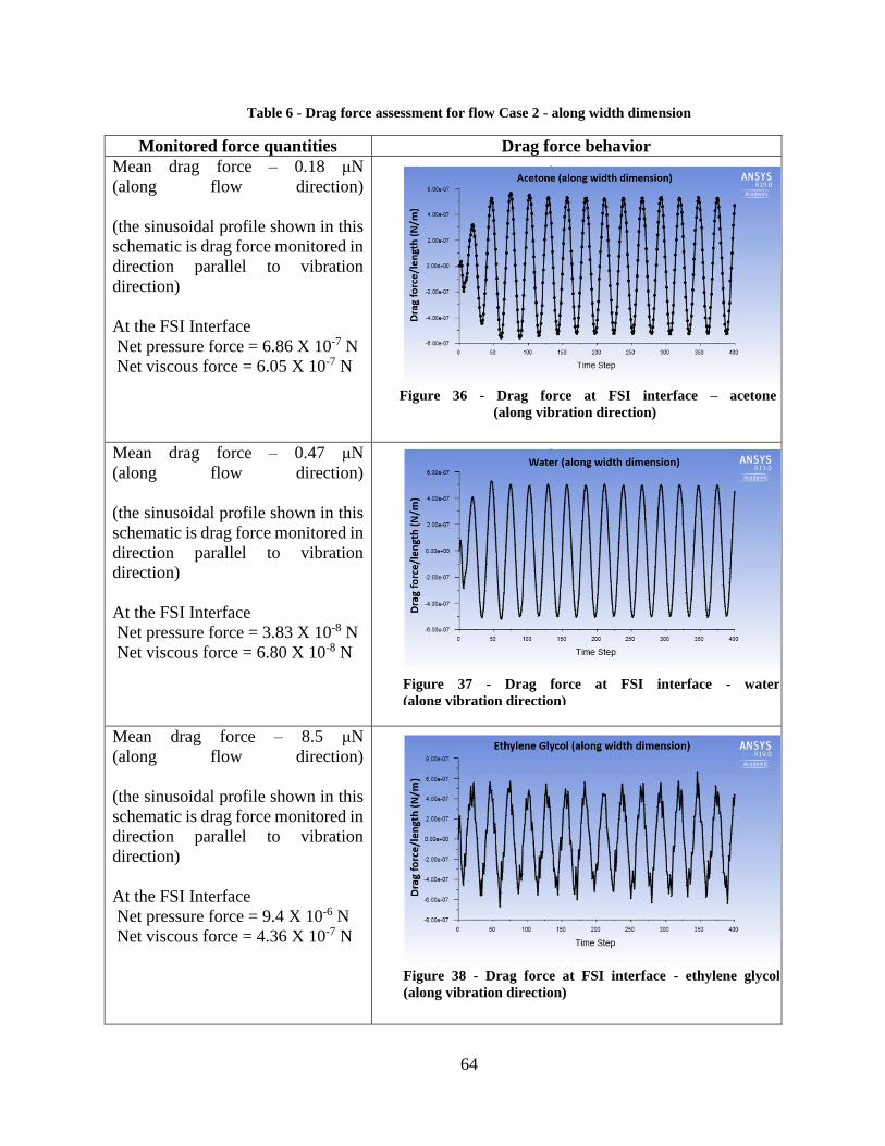
64
Table 6 - Drag force assessment for flow Case 2 - along width dimension
Monitored force quantities Drag force behavior
Mean drag force – 0.18 μN
(along flow direction)
(the sinusoidal profile shown in this
schematic is drag force monitored in
direction parallel to vibration
direction)
At the FSI Interface
Net pressure force = 6.86 X 10⁻⁷ N
Net viscous force = 6.05 X 10⁻⁷ N
Mean drag force – 0.47 μN
(along flow direction)
(the sinusoidal profile shown in this
schematic is drag force monitored in
direction parallel to vibration
direction)
At the FSI Interface
Net pressure force = 3.83 X 10⁻⁸ N
Net viscous force = 6.80 X 10⁻⁸ N
Mean drag force – 8.5 μN
(along flow direction)
(the sinusoidal profile shown in this
schematic is drag force monitored in
direction parallel to vibration
direction)
At the FSI Interface
Net pressure force = 9.4 X 10⁻⁶ N
Net viscous force = 4.36 X 10⁻⁷ N
Figure 36 - Drag force at FSI interface – acetone
(along vibration direction)
Figure 37 - Drag force at FSI interface - water
(along vibration direction)
Figure 38 - Drag force at FSI interface - ethylene glycol
(along vibration direction)
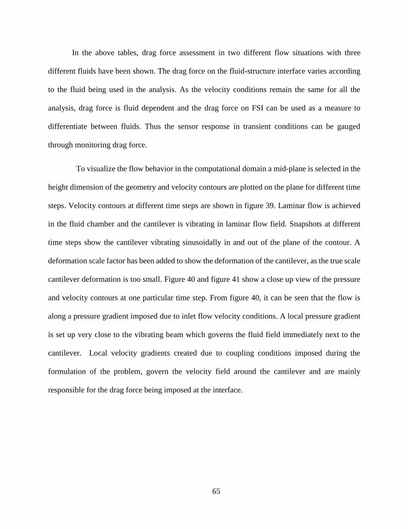
65
In the above tables, drag force assessment in two different flow situations with three
different fluids have been shown. The drag force on the fluid-structure interface varies according
to the fluid being used in the analysis. As the velocity conditions remain the same for all the
analysis, drag force is fluid dependent and the drag force on FSI can be used as a measure to
differentiate between fluids. Thus the sensor response in transient conditions can be gauged
through monitoring drag force.
To visualize the flow behavior in the computational domain a mid-plane is selected in the
height dimension of the geometry and velocity contours are plotted on the plane for different time
steps. Velocity contours at different time steps are shown in figure 39. Laminar flow is achieved
in the fluid chamber and the cantilever is vibrating in laminar flow field. Snapshots at different
time steps show the cantilever vibrating sinusoidally in and out of the plane of the contour. A
deformation scale factor has been added to show the deformation of the cantilever, as the true scale
cantilever deformation is too small. Figure 40 and figure 41 show a close up view of the pressure
and velocity contours at one particular time step. From figure 40, it can be seen that the flow is
along a pressure gradient imposed due to inlet flow velocity conditions. A local pressure gradient
is set up very close to the vibrating beam which governs the fluid field immediately next to the
cantilever. Local velocity gradients created due to coupling conditions imposed during the
formulation of the problem, govern the velocity field around the cantilever and are mainly
responsible for the drag force being imposed at the interface.

66
Figure 39 - Snapshots of velocity contours at the mid-plane of the computational domain for
various time steps
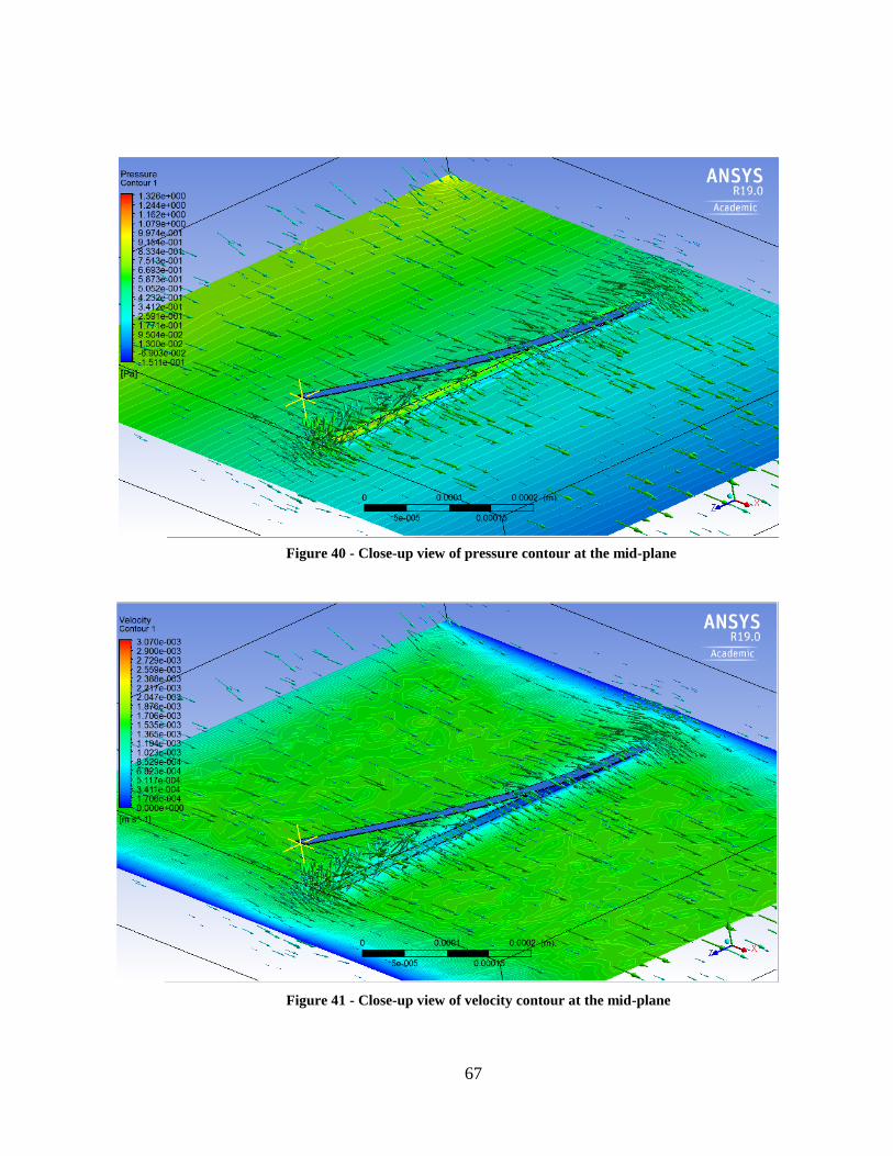
67
Figure 40 - Close-up view of pressure contour at the mid-plane
Figure 41 - Close-up view of velocity contour at the mid-plane
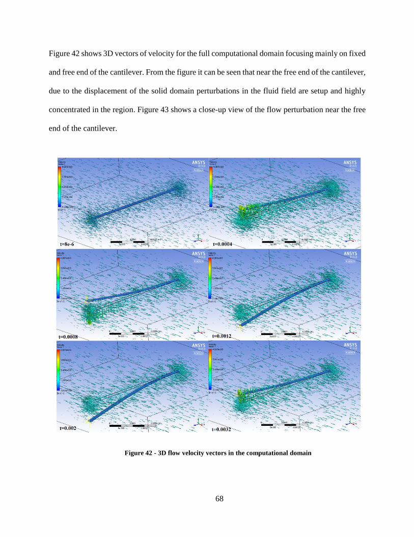
68
Figure 42 shows 3D vectors of velocity for the full computational domain focusing mainly on fixed
and free end of the cantilever. From the figure it can be seen that near the free end of the cantilever,
due to the displacement of the solid domain perturbations in the fluid field are setup and highly
concentrated in the region. Figure 43 shows a close-up view of the flow perturbation near the free
end of the cantilever.
Figure 42 - 3D flow velocity vectors in the computational domain
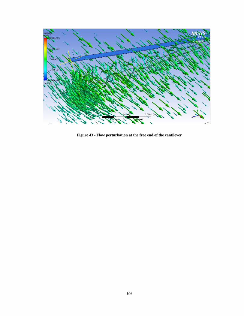
69
Figure 43 - Flow perturbation at the free end of the cantilever
70
Chapter 6
6.1 Conclusions
Detecting biomarkers for Alzheimer’s disease is crucial in understanding the mechanism
and progression of the disease. Aβ1-42 is one of the highly proposed biomarker found in
cerebrospinal fluid which can point towards the level of progression of AD and possible
therapeutic measures. In this regard a MEMS resonator based biosensor is being developed which
incorporates dual detection mechanism: resonance frequency shift based detection and evanescent
wave based fluorescence detection. The behavior of the biosensor under various circumstances
have to be analyzed to optimize the performance and increase reliability of detection.
Computational methods offer advantages in terms of analyzing dynamic behavior of the system,
developing a predictive model for sensor development, design optimization etc., thus reducing cost
and downtime related with manufacturing.
A finite element based computational method using the commercial FEM solver ANSYS
is developed to assess the performance of the biosensor. Fluid-structure interaction is considered
in the finite element model to incorporate the effects of added fluid mass and viscous damping
introduced by the fluid. Frequency domain and time domain approaches are considered for cases
with no net fluid flow and with fluid flow. In a vacuum environment no added mass effect or
damping effects are observed. However, when the biosensor is operating in fluid environment
added mass due to the fluid and viscous damping effects reduce the natural frequency and
resonance frequency of the sensor to lower values. With increasing fluid density and viscosity, the
shift in the frequencies increases and the amplitude response of the sensor also decreases.
Sensitivity of the biosensor is analyzed with mass attachment corresponding to mass range of
amyloid biomarkers. In case of sensor operating in vacuum, for the calculated mass of amyloid
71
biomarkers, a frequency shift of 16.6Hz (S=69.7Hz/ng) is obtained and for the case of sensor
operating in a fluid environment a frequency shift of 0.9Hz (S=3.7Hz/ng) is obtained. With usage
of a phase locked loop (PLL) Doppler vibrometry system a frequency resolution of 0.01Hz can be
obtained. Thus the biosensor being developed is viable in terms of biomarker mass detection.
Using a partitioned algorithm approach available in ANSYS, a time domain transient
analysis of sensor vibrating in a flowing fluid environment is realized. Two velocity conditions
have been imposed in terms of flow direction and drag force applied by the fluid on the sensor is
monitored. The drag force at the fluid-solid interface exhibits a sinusoidal behavior in
correspondence with the sinusoidal motion of the sensor. The mean drag force experienced by the
sensor varies depending on the Reynold’s number of the flow which in turn is a function of density,
viscosity of the fluid and characteristic dimension of the sensor. In case of sensor vibrating in an
acetone environment mean drag force experienced is ~0.2μN and for the case of water and ethylene
glycol the mean drag force being ~0.5μN and ~8μN respectively. Thus assessing drag force serves
as an important parameter in understanding the dynamic behavior of the biosensor. Pressure and
velocity contours help in visualizing the flow field around the sensor area to understand dynamic
effects of flow perturbation due to motion of the sensor.
The finite element analysis results obtained fall under a reasonable error bound. Sources of
error in the frequency domain analysis include errors due to domain discretization and weak
coupling of viscous shear effects in the coupled field elements used to model the contained fluid.
In transient analysis, errors may arise due to larger time steps which may lead to insufficient
convergence of fields. Dynamic meshing technique used to account for deformations in the fluid
domain is also a source of error as parameters corresponding to smoothing of the mesh needed
optimization. Overall this analysis can be used as a preliminary step towards understanding the

72
characteristics of the biosensor and methods can be developed to improve the overall performance
of the sensor.
6.2 Future work
Future work involves simulating the behavior of the sensor in a wide variety of
physiologically relevant fluid systems considering full effect of shear viscosity terms,
thus reducing the error in the analysis.
Effect of local velocity gradients near the vibrating beam have to be addressed rigorously
in order to understand the effect of fluid on biomarker attachment processes.
Further set of analyses include understanding the characteristics of the sensor when its
operating in a non-Newtonian fluid environment so that the performance can be gauged
at physiologically relevant fluid properties.
Integration of optics simulations with mechanical models to gauge the overall response of
the sensor at a point of care diagnostic system level.
Extending the computational approach to an array of sensors that can detect various
biomarkers of interest in a continuous flow arrangement.
Analysis of dynamics and performance of these arrays of biosensors helps develop a better
understanding of design and optimization of array based sensor systems

73
References:
1. https://www.nia.nih.gov/health/alzheimers-disease-fact-sheet
2. https://www.alz.org/facts/overview.asp
3. https://www.alz.org/professionals_and_researchers_13519.asp
4. Smith, M. A., Rottkamp, C. A., Nunomura, A., Raina, A. K. & Perry, G. Oxidative stress in
Alzheimer’s disease. Biochim. Biophys. Acta - Mol. Basis Dis. 1502, 139–144 (2000).
5. Martorana, A., Esposito, Z. & Koch, G. Beyond the cholinergic hypothesis: Do current drugs
work in alzheimer’s disease? CNS Neurosci. Ther. 16, 235–245 (2010).
6. Anatoly Nikolaev, Todd McLaughlin, Dennis O’Leary, and Marc Tessier-Lavigne. APP
Binds DR6 to Cause Axon Pruning and Neuron Death via Distinct Caspases.. Mol.
Neurobiol. 457, 981–989 (2009).
7. Feuerstein, Adam. Merck Alzheimer's Drug Study Halted Early for Futility. New York
City, NY, USA: TheStreet, Inc.(2017)
8. Goedert, M., Spillantini, M. G. & Crowther, R. A. Tau Proteins and Neurofibrillary
Degeneration. Brain Pathol. 1, 279–286 (1991).
9. Iqbal, K. et al. Tau pathology in Alzheimer disease and other tauopathies. Biochim.
Biophys. Acta - Mol. Basis Dis. 1739, 198–210 (2005).
10. Chun, W. & Johnson, G. The role of tau phosphorylation and cleavage in neuronal cell
death. Front. Biosci. a J. virtual … 733–756 (2006)
11. Rashid Deane, Berislav V. Zlokovic, Role of the blood-brain barrier in the pathogenesis of
Alzheimer's disease". Current Alzheimer’s Research 4 (2): 191–7 (2007)
12. Xu, H., Finkelstein, D. I. & Adlard, P. A. Interactions of metals and apolipoprotein e in
Alzheimer’s disease. Front. Aging Neurosci. 6, 1–7 (2014).
13. Cai, Z. & Xiao, M. Oligodendrocytes and Alzheimer’s disease. Int. J. Neurosci. 126, 97–
104 (2016).Cai Z, Xiao M (2016).
14. Reisberg, B. et al. Retrogenesis: clinical, physiologic, and pathologic mechanisms in brain
aging, Alzheimer’s and other dementing processes. Eur. Arch. Psychiatry Clin. Neurosci.
249, S28–S36 (1999).
15. Dougall., Systematic Review of the Diagnostic Accuracy of 99mTc-HMPAO-SPECT in
Dementia. The American journal of geriatric psychiatry, 12(6), 554-. (2004).
74
16. Rabinovici, G. D. & Jagust, W. J. Amyloid imaging in aging and dementia: Testing the
amyloid hypothesis in vivo. Behav. Neurol. 21, 117–128 (2009).
17. Umek, R. M. et al. Electronic detection of nucleic acids: A versatile platform for molecular
diagnostics. J. Mol. Diagnostics 3, 74–84 (2001).
18. Yu, C. J. et al. Electronic detection of single-base mismatches in DNA with ferrocene-
modified probes. J. Am. Chem. Soc. 123, 11155–11161 (2001).
19. C.J. Yu, H. Yowanto, B. Terbrueggen, C. Tao, G.F. Blackburn, Electrochemical detection
of nucleic acids on SAMs-constructed arrays, J. Am. Chem. Soc. 123 11155–11161 (2001).
20. Hwang, M. T. et al. Highly specific SNP detection using 2D graphene electronics and
DNA strand displacement. Proc. Natl. Acad. Sci. 113, 7088–7093 (2016).
21. Fritz, J., Cooper, E. B., Gaudet, S., Sorger, P. K. & Manalis, S. R. Electronic detection of
DNA by its intrinsic molecular charge. Proc. Natl. Acad. Sci. 99, 14142–14146 (2002).
22. Lehmann, M. et al. Simultaneous measurement of cellular respiration and acidification
with a single CMOS ISFET. Biosens. Bioelectron. 16, 195–203 (2001).
23. Suzuki, H., Arakawa, H. & Karube, I. Fabrication of a sensing module using
micromachined biosensors. Biosens. Bioelectron. 16, 725–733 (2001).
24. Shul’ga, A. A. et al. Thin-film conductometric biosensors for glucose and urea
determination. Biosens. Bioelectron. 9, 217–223 (1994).
25. Fernández-Sánchez, C., McNeil, C. J., Rawson, K. & Nilsson, O. Disposable
noncompetitive immunosensor for free and total prostate-specific antigen based on
capacitance measurement. Anal. Chem. 76, 5649–5656 (2004).
26. Fredj, H. Ben et al. Labeled magnetic nanoparticles assembly on polypyrrole film for
biosensor applications. Talanta 75, 740–747 (2008).
27. https://www.illumina.com/
28. www.nanosphere.com.
29. www.affymetrix.com.
30. Urey, H., Timurdogan, E., Ermek, E., Kavakli, I. H. & Alaca, B. E. Mems Biosensor for
Parallel and Highly Sensitive and Specific Detection of Hepatitis. 920–923 (2011).
75
31. Lee, J. H. et al. Immunoassay of prostate-specific antigen (PSA) using resonant frequency
shift of piezoelectric nanomechanical microcantilever. Biosens. Bioelectron. 20, 2157–
2162 (2005).
32. Braun, T. et al. Micromechanical mass sensors for biomolecular detection in a
physiological environment. Phys. Rev. E - Stat. Nonlinear, Soft Matter Phys. 72, 1–9
(2005).
33. Bircher, B. A., Krenger, R. & Braun, T. Automated high-throughput viscosity and density
sensor using nanomechanical resonators. Sensors Actuators, B Chem. 223, 784–790 (2016).
34. https://en.wikipedia.org/wiki/Vibration#Forced_vibration_with_damping
35. Resonant MEMS: Fundamentals, Implementation and Application, (2015)
DOI:10.1002/9783527676330
36. Green, C. P. & Sader, J. E. Frequency response of cantilever beams immersed in viscous
fluids with applications to the atomic force microscope. J. Appl. Phys. 92, 6262–6274
(2002).
37. El Hami, A. & Radi, B. Fluid-Structure Interactions and Uncertainties. (2017).
doi:10.1002/9781119388937
38. Fedder, G. K. MEMS fabrication. Int. Test Conf. 2003. Proceedings. ITC 2003. 1, (2003).
39. Bashir, R. BioMEMS: State-of-the-art in detection, opportunities and prospects. Adv. Drug
Deliv. Rev. 56, 1565–1586 (2004).
40. Schwarzer, N. & Richter, F. On the Determination of Film Stress from Substrate Bending:
STONEY’s Formula and Its Limits. Whitepaper 1–17 (2006).
41. Timoshenko, S. and Young, D.H. Vibration Problems in Engineering, 3rd edn, Van
Nostrand Company, Inc., New York. (1955)
42. Heinrich, S. M. & Dufour, I. Fundamental Theory of Resonant MEMS Devices. Reson.
MEMS Princ. Model. Implementation, Appl. 1–28 (2015).
doi:10.1002/9783527676330.ch1
43. Braun, T. et al. Micromechanical mass sensors for biomolecular detection in a
physiological environment. Phys. Rev. E - Stat. Nonlinear, Soft Matter Phys. 72, 1–9
(2005).
44. Grandmont, C. Fluid-Structure Interaction : A Theoretical Point of View. 6559, 1–1 (2017).

76
45. ANSYS® Academic Research Mechanical, Release 19.1, Help System, ACT Acoustics
analysis guide v190.1, Introduction to acoustics, ANSYS, Inc.
46. ANSYS® Academic Research Fluids, Release 16.1, Help System, FSI Analysis guide, FSI
overview, ANSYS, Inc.
47. ANSYS® Academic Research Fluids, Release 16.0, Help System, FSI Analysis guide, Co-
simulation, Geometry and Meshing overview, ANSYS, Inc.
48. ANSYS® Academic Research Mechanical, Release 19.1, Help System, ACT Piezo and
MEMS analysis guide v180.1, Piezo and MEMS, ANSYS, Inc.
49. Beer,F., Johnston, E.r., DeWolf, J., and Mazurek, D. Mechanics of Materials, 6th edn,
McGraw-Hill, New York (2011)