Computation of Time-Periodic Solutions of the Benjamin-Ono

Computation of Time-Periodic Solutions of the

Benjamin-Ono Equation

David M. Ambrose ∗ Jon Wilkening †

July 2, 2009

Abstract

We present a spectrally accurate numerical method for finding non-trivial time-periodic solutions of non-linear partial differential equations. The method is basedon minimizing a functional (of the initial condition and the period) that is positiveunless the solution is periodic, in which case it is zero. We solve an adjoint PDE tocompute the gradient of this functional with respect to the initial condition. We includeadditional terms in the functional to specify the free parameters, which, in the case ofthe Benjamin-Ono equation, are the mean, a spatial phase, a temporal phase and thereal part of one of the Fourier modes at t = 0.

We use our method to study global paths of non-trivial time-periodic solutions con-necting stationary and traveling waves of the Benjamin-Ono equation. As a startingguess for each path, we compute periodic solutions of the linearized problem by solvingan infinite dimensional eigenvalue problem in closed form. We then use our numericalmethod to continue these solutions beyond the realm of linear theory until another trav-eling wave is reached. By experimentation with data fitting, we identify the analyticalform of the solutions on the path connecting the one-hump stationary solution to thetwo-hump traveling wave. We then derive exact formulas for these solutions by explic-itly solving the system of ODEs governing the evolution of solitons using the ansatzsuggested by the numerical simulations.

∗Department of Mathematical Sciences, Clemson University, Clemson, SC 29634. Current address: De-

partment of Mathematics, Drexel University, Philadelphia, PA 19104 ([email protected]). This

work was supported in part by the National Science Foundation through grant DMS-0926378.†Department of Mathematics and Lawrence Berkeley National Laboratory, University of California,

Berkeley, CA 94720 ([email protected]). This work was supported in part by the Director, Of-

fice of Science, Computational and Technology Research, U.S. Department of Energy under Contract No.

DE-AC02-05CH11231.

1

2 David M. Ambrose and Jon Wilkening

Key words. Periodic solutions, Benjamin-Ono equation, non-linear waves, solitons,

bifurcation, continuation, optimal control, adjoint equation, spectral method

AMS subject classifications. 65K10, 37M20, 35Q53, 37G15

1 Introduction

A fundamental problem in the theory of ordinary and partial differential equations is to

determine whether the equation possesses time-periodic solutions. Famous examples of

ordinary differential equations with periodic solutions include the Brusselator [FB85, Gov00,

Str00] and the three-body problem [Are63, HNW00]. In partial differential equations, time-

periodic solutions can be “trivial” stationary or traveling waves, or can be genuinely time-

periodic. Such a problem can be studied in either the forced or unforced context. Forced

problems include an external force in the PDE that is time-periodic; solutions with the

same period are then sought. In the unforced problem, the period is one of the unknowns.

In this work, we present a numerical method for finding genuinely time-periodic solutions of

the unforced Benjamin-Ono equation with periodic boundary conditions. These solutions

have many remarkable properties, which we will describe.

Our work is motivated by the calculations of Hou, Lowengrub, and Shelley for the vortex

sheet with surface tension [HLS94, HLS97], and by the analysis of Plotnikov, Toland and

Iooss [PT01, IPT05] for the water wave. Hou, Lowengrub, and Shelley developed an efficient

numerical method to solve the initial value problem for the vortex sheet with surface tension.

They performed calculations for a variety of initial conditions and values of the surface

tension parameter, and found many situations in which the solutions appear to be close to

time-periodic. They did not, however, try to measure the deviation from time-periodicity

or attempt to vary the initial conditions to reduce this deviation. Plotnikov, Toland, and

Iooss have proved the existence of time-periodic water waves, without surface tension, in

the case of either finite or infinite depth. This is proved using a version of the Nash-Moser

implicit function theorem. Their work includes no computation of the water waves. We aim

to get a firmer handle on these solutions with an explicit calculation. To this end, in the

present work, we develop a general numerical method for finding time-periodic solutions of

nonlinear systems of partial differential equations and eventually plan to use this method

for the vortex sheet and water wave problems. In fact, during the review process of the

present work, we have succeeded in computing several families of time-periodic solutions of

the vortex sheet with surface tension [AW09].

The Benjamin-Ono equation, developed in [Ben67, DA67, Ono75], is a model equation

Time-Periodic Solutions of the Benjamin-Ono Equation 3

for the evolution of waves on deep water. It is a widely-studied dispersive equation, and

much is known about solutions. It would be impossible to mention all results on Benjamin-

Ono, but we mention, for example, that weak solutions exist for u0 ∈ L2 [Sau79, GV91],

and that the solution exists for all time if u0 ∈ H1 [Tao04]. We chose the Benjamin-Ono

equation as a first application for our numerical method because it is much less expensive

to evolve than the vortex sheet or water wave, yet has many features in common with them,

such as non-locality (due to the Hilbert transform in the former case and the Birkhoff-Rott

integral in the latter two cases.) In our numerical simulations, we find that the Benjamin-

Ono equation has a rich family of non-trivial time-periodic solutions that act as rungs in

a ladder connecting traveling waves with different speeds and wavelengths by creating or

annihilating oscillatory humps that grow or shrink in amplitude until they become part of

the stationary or traveling wave on the other side of the rung. The dynamics of these non-

trivial solutions are often very interesting, sometimes resembling a low amplitude traveling

wave superimposed on a larger carrier signal, and other times looking like a collection of

interacting solitons that pass through each other or bounce off each other, depending on

their relative amplitudes.

By fitting our numerical data, we have determined that all the solutions we have com-

puted are special cases of the multi-phase solutions studied by Case [Cas79], Satsuma and

Ishimori [SI79], Dobrokhotov and Krichever [DK91], and Matsuno [Mat04], but with special

initial conditions (that yield periodic orbits) and a modified mean (to change their speeds

and allow bifurcations to occur between different levels of the hierarchy of multi-phase so-

lutions). We did not take advantage of this structure when we developed our numerical

method; hence, our approach can also be used for non-integrable problems. We also note

that bifurcation within the family of multi-phase solutions has not previously been dis-

cussed in the literature, nor has the remarkable dynamics of the Fourier coefficients of these

solutions beyond the original derivation by Benjamin [Ben67] of the form of the traveling

waves for this equation.

We are aware of very few works on the existence of time-periodic solutions for water

wave model equations. Crannell has demonstrated [Cra96] the existence of periodic, non-

traveling, weak solutions of the Boussinesq equation using a generalization of the mountain

pass lemma of Rabinowitz. Chen and Iooss have proved existence of time-periodic solutions

in a two-way Boussinesq-type water wave model [CI05]. As in [PT01] and [IPT05], there is

no computation of the solution in either of these studies. Cabral and Rosa have recently

discovered a period-doubling cascade of periodic solutions for a damped and forced version

of the Korteweg–de Vries equation [CR04]. They use a Fourier pseudospectral method for

the spatial discretization and a first order semi-implicit scheme in time. To find periodic


solutions, they use a secant method on a numerical Poincare map. Whereas our approach

is based on minimizing a functional that measures deviation from periodicity, they rely on

the stability of the orbit to converge to a periodic solution. They stop when they find

a solution that returns to within one percent of its initial state, whereas we resolve our

periodic solutions to 13-15 digits of accuracy, which allows us to study the analytic form of

the solutions.

Water waves aside, many authors have investigated time-periodic solutions of other par-

tial differential equations both numerically and analytically. For instance, Smiley proves

existence of time-periodic solutions of a nonlinear wave equation on an unbounded domain

[Smi89]; he also develops a numerical method for the same problem [Smi90]. On a finite do-

main, Brezis uses duality principles to prove the existence of periodic solutions of nonlinear

vibrating strings in both the forced and unforced setting; see [Bre83]. Mawhin has written

a survey article on periodic solutions of semilinear wave equations [Maw95], which includes

many references. Pao has developed a numerical method for the solution of time-periodic

parabolic boundary-value problems [Pao01]. Pao gives various iterative schemes, but unlike

the present work, these are not based on variational principles or the dual system. Brown

et. al. [BKOR92] have used the popular software package AUTO [DKK91a] to study Hopf

bifurcation and loss of stability for traveling waves of the regularized Kuramoto-Sivashinsky

equation. They observe modulated traveling waves similar to many of the solutions we have

found for Benjamin-Ono. And of course, time-periodic solutions of systems of ordinary

differential equations have also been widely studied, e.g. in [Rab78, Rab82, Zeh83, Dui84].

The most popular methods for the numerical solution of boundary value problems gov-

erned by ODEs, which include finding time-periodic solutions as a special case, are orthog-

onal collocation methods [DKK91b] and shooting/multi-shooting methods [SB02]. These

methods can also be used for PDEs via the method of lines, i.e. by discretizing space first to

obtain an ODE. Orthogonal collocation methods (such as implemented in AUTO) require

a nonlinear system of equations to be solved involving all the degrees of freedom at every

timestep. In many of our simulations, the solution at every timestep cannot even be stored

simultaneously in memory; hence, it would be impossible to solve a system of equations for

all these variables. For PDEs, shooting methods are also very expensive as the Jacobian of

the functional measuring errors in the boundary conditions must be computed with respect

to variation of the N “unknown” initial conditions, which is N times more expensive than

computing the functional itself.

Lust and Roose [LR96] propose an interesting solution to this problem in which a shoot-

ing method is used for some of the degrees of freedom while iteration on a Poincare map

is used for the other degrees of freedom. They aim to exploit the fact that many high


dimensional systems actually exhibit low-dimensional dynamical behavior. In the present

work, we offer an alternative strategy based on the following idea: while the Jacobian of the

residual measuring error in each of the boundary conditions is expensive to compute, the

gradient of the sum of squares of this residual can be computed by solving a single adjoint

PDE. Although the full Jacobian gives more information, it is N times more expensive to

compute. We find that it is more efficient to use a quasi-Newton method with only the

gradient information than it is to use a full Newton method with the Jacobian. This ap-

proach is not restricted to finding time-periodic solutions; it will work for any boundary

value problem. Also, although we have not tried it, our method can be easily adapted to

incorporate the idea behind multi-shooting methods, namely that by introducing “interior”

initial conditions and boundary conditions, we can avoid a great deal of the ill conditioning

due to nearby trajectories diverging exponentially in time.

The closest numerical method to our own that we have found is due to Bristeau, Glowin-

ski and Periaux [BGP98], who developed a least squares shooting method for numerical

computation of time-periodic solutions of linear dynamical systems with applications in

scattering phenomena in two and three dimensions; see also [GR06]. These authors employ

methods of control theory to compute variational derivatives, and although they only apply

their methods to linear problems, they mention that their techniques will also work on non-

linear problems. Our method can be considered an extension of their approach that focuses

on the difficulties that arise due to non-linearity. In particular, we replace their conjugate

gradient solver with a black-box minimization algorithm, (the BFGS method [NW99]), and

include an additional penalty function to prescribe the values of the free parameters that

describe the manifold of non-trivial time-periodic solutions. Without this penalty function,

the basic method is only found to produce constant solutions and traveling waves.

This paper is organized as follows: In Section 2, we discuss spatially periodic stationary

and traveling solutions of the Benjamin-Ono equation, the bifurcations from constant so-

lutions to traveling waves, and the pole dynamics of meromorphic solutions. In Section 3,

we investigate time-periodic solutions of the linearized Benjamin-Ono equation; this is the

linearization about the stationary solutions discussed previously. To analyze the linearized

problem, we compute (numerically) the spectrum and eigenfunctions of the relevant linear

operator and deduce their analytic form by trial and error; the resulting formulas can be

verified rigorously (but we omit details).

In Section 4, we describe our numerical method, which involves minimizing a non-

negative functional that is zero if and only if the solution is periodic. We solve an adjoint

PDE to compute the variational derivative of this functional with respect to perturbation of

the initial condition and use the BFGS minimization algorithm to minimize the functional.


The Benjamin-Ono and adjoint equations are solved with a pseudo-spectral collocation

method using a fourth order, semi-implicit Runge-Kutta scheme. We use a penalty function

to rule out constant solutions and traveling waves, and to prescribe the free parameters of

the manifold of non-trivial solutions. We then vary a bifurcation parameter to study the

global properties of these non-trivial solutions. In the present work, we apply this method

only to the Benjamin-Ono equation, but we are confident that this method is applicable to

virtually any system of partial differential equations that possesses time-periodic solutions.

In Section 5, we use our method to study the global behavior of non-trivial time-periodic

solutions far beyond the realm of validity of the linearization about stationary and traveling

waves. We will follow one such path to discover that the one-hump stationary solution is

connected to the two-hump traveling wave by a path of non-trivial time periodic solutions.

In Section 6, we re-formulate the ODE governing the evolution of poles to reveal an exact

formula for the solutions on the path studied numerically in Section 5. Thus, unexpectedly,

we have proved that non-trivial time-periodic solutions bifurcate from stationary solutions

by exhibiting a family of them explicitly. In a follow-up paper [AW], we will classify all

bifurcations from traveling waves, study the paths of non-trivial solutions connecting several

of them, propose a conjecture explaining how they all fit together, and describe their analytic

form to the extent that we are able. We end with a few concluding remarks in Section 7.

2 Stationary, Traveling and Soliton Solutions

We consider the spatially periodic Benjamin-Ono equation with the following sign conven-

tion:

ut = Huxx − uux. (1)

Of course, the operator H is the Hilbert transform. Recall that the symbol of H is H(k) =

−i sgn(k). Many authors include a factor of two in the convection term and place a minus

sign in front of H. The former change causes solutions to be scaled by a factor of 1/2 while

the latter change has no effect as H is defined with the opposite sign with this convention.

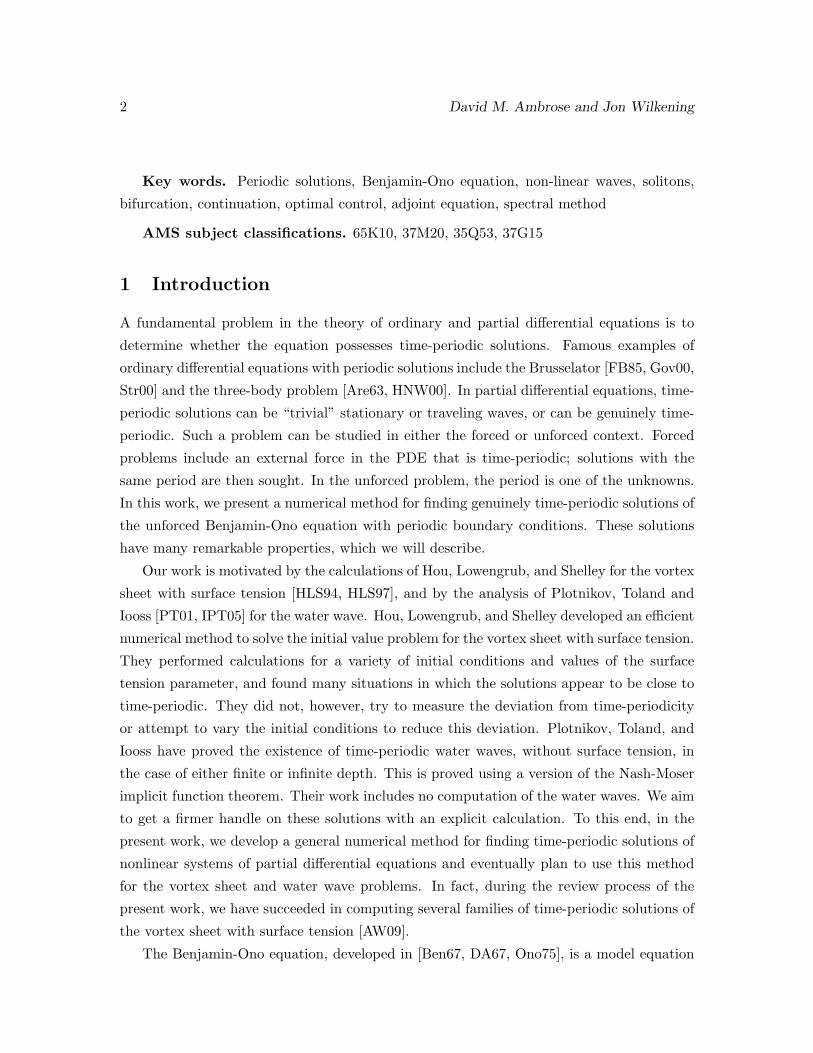
This equation possesses a two-parameter family of stationary solutions, namely

u(x) =1− 3β2

1− β2+

4β[cos(x− θ)− β]1 + β2 − 2β cos(x− θ)

, (−1 < β < 1, θ ∈ R). (2)

These solutions have mean α, related to β via

α(β) =1− 3|β|2

1− |β|2, |β|2 =

1− α

3− α. (3)


0

−2

0

2

4

6

8

π 2π

Stationary Solutions

x

u

α = 1

α = −0.8225

α = 0.544375

αk = 1 − (3k/40)2, k=0..18

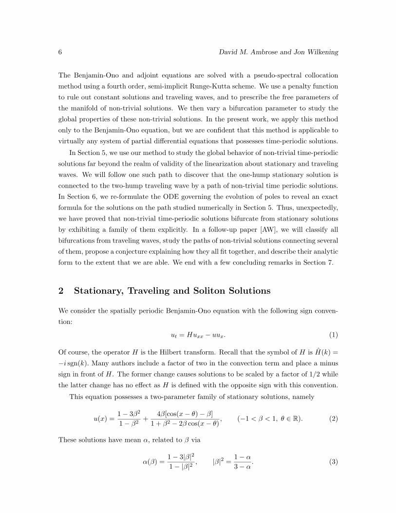
Figure 1: Stationary solutions of the Benjamin-Ono equation.

Changing the sign of β is equivalent to the phase shift θ → θ − π. It is convenient to

complexify β and define uβ to be the mean-zero part of (2) with β → |β|, θ → arg β:

stationary solution = α(β) + uβ(x), β = |β|e−iθ ∈ ∆ = {z ∈ C : |z| < 1}. (4)

Note that the subscript β does not indicate a derivative here. Several stationary solutions

with β real and negative are shown in Figure 1. The Fourier representation of uβ is simply

uβ,k =

2β|k|, k < 0

0, k = 0

2βk, k > 0

, (5)

where β is the complex conjugate of β. These functions uβ(x) are the building blocks for

the meromorphic solutions discussed below.

Note that the constant solution u ≡ α0 is also a stationary solution, as are the re-scaled

solutions

uN,β(x) = Nα(β) + Nuβ(Nx), (β ∈ ∆, N = 1, 2, 3, . . . ),

which have mean α0 = Nα(β). If we restrict attention to stationary solutions with even

symmetry (i.e. with β real), we find that there is a pitchfork bifurcation at each positive

integer (using the mean as a bifurcation parameter). As α0 changes from N+ to N−, the

constant solution splits, yielding two additional (N -hump stationary) solutions, namely


uN,β(x) with β = 0±. The pitchfork would be obtained by plotting the real part of the

Nth Fourier mode versus the mean, where we observe that the Fourier representation of

u = uN,β (for any β ∈ ∆) is given by

uk =

Nα(β), k = 0,

2Nβk/N , k ∈ NZ, k > 0,

2Nβ|k|/N , k ∈ NZ, k < 0,

0 otherwise.

(6)

If we do not restrict attention to even solutions, the phase shift θ acts as a second parameter

connecting the two outer branches of the pitchfork into a two-dimensional, bowl-shaped

sheet (plotting the real and imaginary parts of the Nth Fourier mode versus the mean).

In the bifurcation problem just described, we varied the mean α0 and found bifurcations

from constant solutions to stationary solutions at the positive integers. The remainder of

this paper deals with bifurcation from these stationary solutions to non-trivial time-periodic

solutions and their global continuation beyond the realm of linear theory. Rather than

varying the mean, we will hold α0 ∈ R constant and use another quantity (such as the

period T or the real part of one of the Fourier modes of u at t = 0) as the bifurcation

parameter. As a first step, let us consider bifurcation from constant solutions to traveling

waves holding α0 ∈ R constant and varying T .

All traveling wave solutions of the Benjamin-Ono equation can be found by applying

a simple transformation to a stationary solution, and vice versa. Indeed, if u(x, t) is any

solution of (1), then

U(x, t) = u(x− ct, t) + c (7)

is also a solution; thus, adding a constant c to a stationary solution causes it to travel to

the right with speed c. We can parametrize these N -hump traveling waves by their mean

α0 ∈ R and decay/phase parameter β ∈ ∆:

uα0,N,β(x, t) = uN,β(x− ct) + c,(c = α0 −Nα(β)

). (8)

If we express the period T = 2π/(N |c|) in terms of β and solve for β, we find that we can

bifurcate from any constant solution u ≡ α0 to an N -hump traveling solution with the same

mean. If α0 < N , a pitchfork from the constant solution occurs at T0 = 2π/[N(N − α0)];

as we increase T from T0 to ∞, α = [2π/(NT ) + α0]/N decreases from 1 to α0/N and

|β| varies from 0 to√

(1− α0/N)/(3− α0/N). Similarly, if α0 > N , a pitchfork occurs at

T0 = 2π/[N(α0 − N)]; as we decrease T from T0 to 0, α = [α0 − 2π/(NT )]/N decreases

from 1 to −∞, and |β| varies from 0 to 1. And if α0 = N , the situation is qualitatively


similar to the latter case, but the pitchfork occurs at T0 =∞, i.e. all three solutions (with

β real) exist for any period T > 0.

We remark that if the traveling waves described above have zero mean, they are a special

case of the meromorphic N -particle “periodic soliton” solutions described in [Cas78], namely

u(x, t) = 2 Re

{N∑

l=1

2ei[x+t−xl(t)] − 1

},

where Im{xl(0)} > 0 and the xl(t) satisfy the system of differential equations

dxl

dt=

N∑m=1m6=l

2e−i(xm−xl) − 1

+N∑

m=1

2e−i(xl−xm) − 1

, (1 ≤ l ≤ N). (9)

In our notation, we write

xl(t) = i log βl(t) = θl(t)− i log |βl(t)|, (βl = |βl|e−iθl = e−ixl)

and generalize to the case that the mean α0 can be non-zero. We find from (9) and (7) that

u(x, t) = α0 +N∑

l=1

uβl(t)(x) (10)

is a solution of (1) if the variables βl ∈ ∆ satisfy

βl =N∑

m=1m6=l

−2iβ2l

βl − βm+

N∑m=1

2iβ2l

βl − β−1m

+ i(2N − 1− α0)βl, (1 ≤ l ≤ N). (11)

The N -hump traveling wave then has the representation

uα0,N,β(x, t) = α0 +N∑

l=1

uβl(t)(x), βl(t) = N√

βe−ict, c = α0 −Nα(β),

where each βl is assigned a distinct Nth root of β. As we are interested in developing

numerical methods that generalize to more complicated systems such as the vortex sheet

with surface tension and the water wave, we do not exploit the existence of meromorphic

solutions in our numerical method; however, the non-trivial time-periodic solutions we find

do turn out to be of this form; see Section 6.

3 Linear Theory

We formulate the problem of finding time-periodic solutions of the Benjamin-Ono equation

as that of finding an initial condition u0 and period T such that F (u0, T ) = 0, where


F : H1 × R→ H1 is given by

F (u0, T ) = u(·, T )− u0, ut = Huxx − uux, u(·, 0) = u0. (12)

Clearly, stationary solutions are periodic with any period T . In this section, we linearize

F about these stationary solutions and use solutions of the linearized problem as initial

search directions to find time-periodic solutions of the nonlinear problem. Bifurcation from

traveling waves can be reduced to this case by adding an appropriate constant and requiring

that the period of the perturbation coincide with the period of the traveling wave (although

there may be a phase shift involved as well). We present a detailed analysis of the traveling

case in [AW].

3.1 Linearization About Stationary Solutions

Let u = uN,β be an arbitrary N -hump stationary solution. If u(x) + v(x, t) is to satisfy (1)

to first order in v, then v should satisfy

vt = Hvxx − (uv)x. (13)

(The exact solution satisfies vt = Hvxx − (uv)x − vvx.) Equation (13) can be written

vt = iBAv, (14)

where the (unbounded, self-adjoint) operators A and B on H1 are defined as

A = H∂x − u, B =1i∂x. (15)

To solve (14), we are interested in the eigenvalue problem

BAz = ωz, (16)

so that if BA has a complete set of eigenvectors, the general solution of (14) will be a

superposition of functions of the form

v(x, t) = Re{Cz(x)eiωt}, C ∈ C.

Of course, the eigenvalues of a composition of Hermitian operators need not be real, but for

A and B in (15), we can compute all the eigenvalues explicitly, and they are indeed real.

We do this numerically (which surprisingly leads us to formulas we can check analytically)

by truncating the Fourier representations of A and B and computing the eigenvalues of the

matrix BA. More precisely, we choose a cutoff frequency K (e.g. K = 240) and define the

(2K − 1)× (2K − 1) matrices

Akl = |k|δkl − uk−l = |k|δkl − ul−k, Bkl = kδkl, (−K < k, l < K), (17)


where uk was given in (6) and δkl = 1 if k = l and 0 otherwise. By carefully studying the

eigenvalues for different values of N and β = −√

(1− α)/(3− α) with α < 1, we determined

that

ωN,n =

−ωN,−n n < 0,

0 n = 0,

(n)(N − n) 1 ≤ n ≤ N − 1,

(n + 1−N)(n + 1 + N(1− α)

)n ≥ N.

(18)

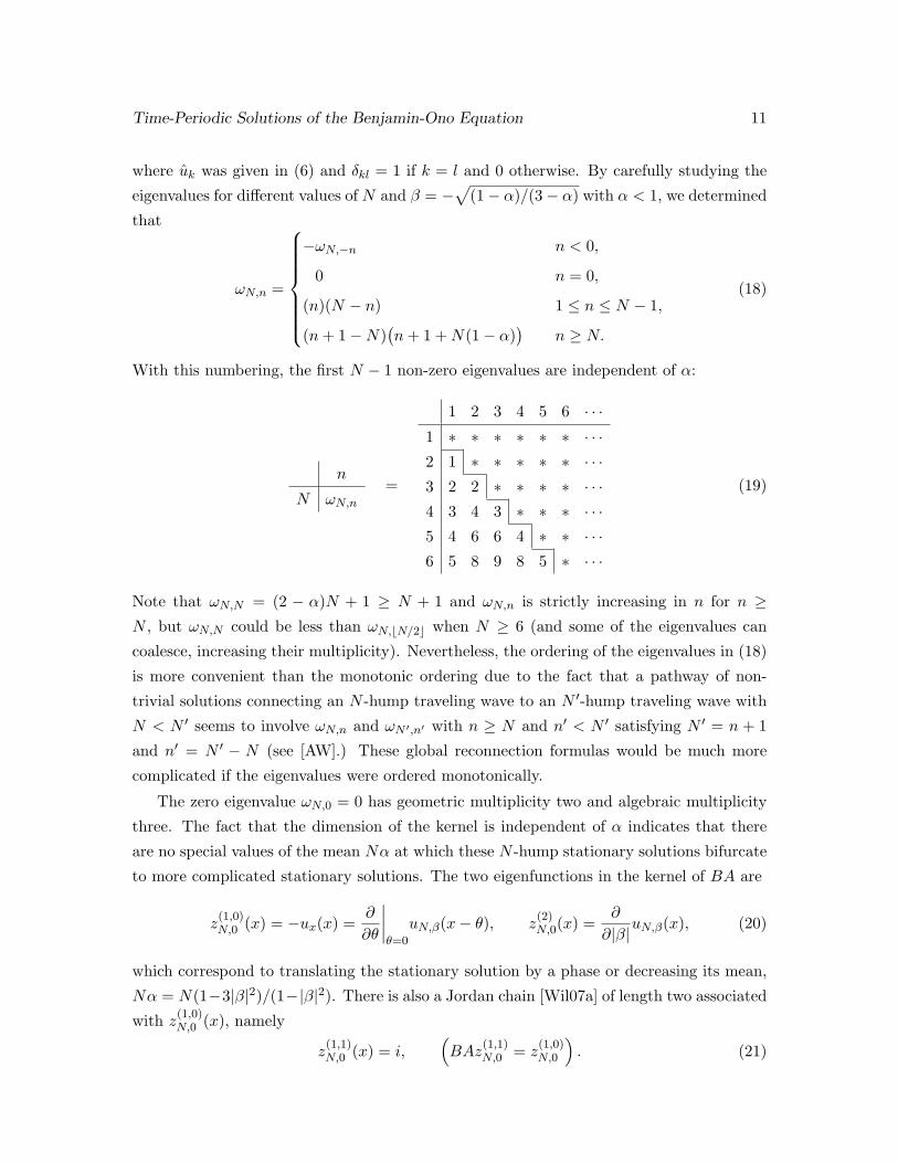
With this numbering, the first N − 1 non-zero eigenvalues are independent of α:

n

N ωN,n

=

1 2 3 4 5 6 · · ·1 ∗ ∗ ∗ ∗ ∗ ∗ · · ·2 1 ∗ ∗ ∗ ∗ ∗ · · ·3 2 2 ∗ ∗ ∗ ∗ · · ·4 3 4 3 ∗ ∗ ∗ · · ·5 4 6 6 4 ∗ ∗ · · ·6 5 8 9 8 5 ∗ · · ·

(19)

Note that ωN,N = (2 − α)N + 1 ≥ N + 1 and ωN,n is strictly increasing in n for n ≥N , but ωN,N could be less than ωN,bN/2c when N ≥ 6 (and some of the eigenvalues can

coalesce, increasing their multiplicity). Nevertheless, the ordering of the eigenvalues in (18)

is more convenient than the monotonic ordering due to the fact that a pathway of non-

trivial solutions connecting an N -hump traveling wave to an N ′-hump traveling wave with

N < N ′ seems to involve ωN,n and ωN ′,n′ with n ≥ N and n′ < N ′ satisfying N ′ = n + 1

and n′ = N ′ − N (see [AW].) These global reconnection formulas would be much more

complicated if the eigenvalues were ordered monotonically.

The zero eigenvalue ωN,0 = 0 has geometric multiplicity two and algebraic multiplicity

three. The fact that the dimension of the kernel is independent of α indicates that there

are no special values of the mean Nα at which these N -hump stationary solutions bifurcate

to more complicated stationary solutions. The two eigenfunctions in the kernel of BA are

z(1,0)N,0 (x) = −ux(x) =

∂

∂θ

∣∣∣∣θ=0

uN,β(x− θ), z(2)N,0(x) =

∂

∂|β|uN,β(x), (20)

which correspond to translating the stationary solution by a phase or decreasing its mean,

Nα = N(1−3|β|2)/(1−|β|2). There is also a Jordan chain [Wil07a] of length two associated

with z(1,0)N,0 (x), namely

z(1,1)N,0 (x) = i,

(BAz

(1,1)N,0 = z

(1,0)N,0

). (21)


The corresponding solution of (14) is

v(x, t) = −iz(1,1)N,0 (x) + tz

(1,0)N,0 (x) = 1− tux(x) =

∂

∂ε

∣∣∣∣ε=0

[u(x− εt) + ε],

i.e. this linear growth mode arises due to the fact that adding a constant to a stationary

solution causes it to travel. The multiple eigenvalues ωN,n = ωN,N−n with 1 ≤ n ≤ N − 1

pose a minor obstacle to obtaining explicit formulas for the eigenvectors. We eventually

realized that because the shift operator

Sθz(x) = z(x− θ), Sθ,kl = e−ikθδkl, θ = 2π/N (22)

commutes with BA, the eigenspaces of BA are invariant under the action of Sθ. Thus we

can impose the additional requirement that if z is an eigenvector of BA corresponding to a

multiple eigenvalue, then z should also satisfy

zk 6= 0 and zl 6= 0 ⇒ k − l ∈ NZ, (23)

i.e. the non-zero Fourier coefficients are equally spaced with stride length N . Using this

condition to make the eigenvectors unique up to scaling, we were able to recognize the

patterns that emerge in the numerical eigenvectors (with the exception of the coefficient C

and the j = 0 case when n ≥ N , which we determined analytically):

zN,n,k

∣∣∣k=n+jN

=

(1 + N(|j|−1)

N−n

)β|j|−1 j < 0

C(1 + Nj

n

)βj+1 j ≥ 0

,

( 1 ≤ n ≤ N − 1

C = −nN

(N−n)[n+(N−n)|β|2

])

,

zN,n,k

∣∣∣k=n−N+1+jN

=

0 j < 0

−β(1−|β|2)2

[1−

(1− N

n+1

)|β|2

]j = 0(

1 + N(j−1)n+1

)βj−1 j ≥ 1

, (n ≥ N). (24)

These formulas can be summed to obtain zN,n(x) as a rational function of eix, but we prefer

to work with the Fourier coefficients. Note that as n → ∞ (holding N fixed), the index

k = n − N + 1 of the first non-zero Fourier mode increases to infinity. The eigenvectors

corresponding to negative eigenvalues ωN,−n with n ≥ 1 satisfy zN,−n(x) = zN,n(x), so

the Fourier coefficients appear in reverse order, conjugated: zN,−n,k = zN,n,−k. When β

is real, the Fourier coefficients are real and zN,−n(x) = zN,n(−x). We have verified the

formulas (18) and (24) analytically, and can also prove that the Fourier representation of

these eigenvectors (together with the associated vector corresponding to the Jordan chain)

form a Riesz basis for `2(Z); hence, we have not missed any eigenvalues.


3.2 Bifurcation from Stationary Solutions

Now that we have solved the eigenvalue problem for BA, we can compute the derivative

of the operator F in (12) above. We continue to assume that u is an N-hump stationary

solution so that DF = (D1F,D2F ) : H1 × R→ H1 satisfies

D1F (u, T )v0 =∂

∂ε

∣∣∣ε=0

F (u + εv0, T ) = v(·, T )− v0 =[eiBAT − I

]v0,

D2F (u, T )τ =∂

∂ε

∣∣∣ε=0

F (u, T + ετ) = 0.

(25)

Note that v0 ∈ ker D1F (u, T ) iff the solution v(x, t) of the linearized problem is periodic

with period T . These solutions of the linearized problem serve as initial search directions in

which to find periodic solutions of the non-linear problem. Since D2F = 0 in the stationary

case, the nullspace N of DF = (D1F,D2F ) is of the form N = N1×R where N1 = kerD1F .

A basis for N1 consists of the functions

v0(x) = Re{zN,n(x)} and v0(x) = Im{zN,n(x)}, (26)

where n ranges over all integers such that

ωN,nT ∈ 2πZ. (27)

Negative values of n have already been accounted for in (26) using zN,−n(x) = zN,n(x). The

n = 0 case always yields two vectors in the kernel, namely those in (20). These directions

do not cause bifurcations as they lead to other stationary solutions in the two parameter

family. Thus, the periods at which bifurcations are expected are

TN,n,m =2πm

ωN,n, (m,n ≥ 1). (28)

Note that this set is dense on the positive real line since ωN,n → ∞ as n → ∞. This

leads to a small divisor problem when trying to apply the Liapunov-Schmidt reduction

[GS85, Kie04] to rigorously analyze bifurcations in the set of solutions of the equation

F (u0, T ) = 0. For other problems, small divisors have been dealt with successfully using

Nash-Moser theory; see e.g. [Nir01, PT01, IPT05]. As most of the bifurcations responsible

for the small divisor problem involve high frequency perturbations that are smoothed out

by the numerical discretization, we have not found small divisors to cause major difficulties

in our ability to track paths of time-periodic solutions.

In our numerical studies, we have found that each of the eigenfunctions zN,n(x) with

n ≥ 1 gives a direction along which a sheet of non-trivial solutions bifurcates from the N -

hump stationary solution. More precisely, if we let a parameter ε → 0, there appear to be


12.5 12.6 12.7 12.8 12.9 13 13.10

1

2

3

4

5

6

7

8

ampl

itude

T

Amplitude of traveling wave versus period

α0 = 1/2

n = 1

n = 2

n = 7

4π

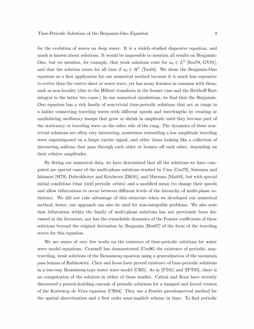
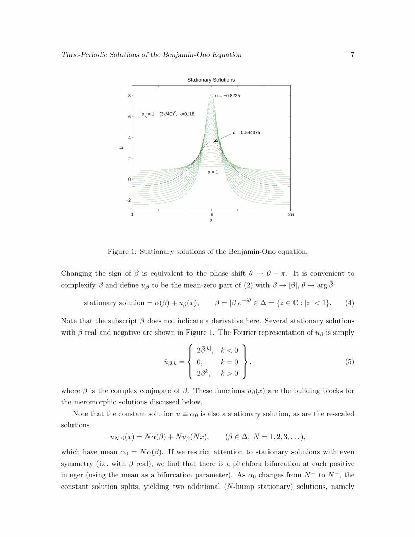
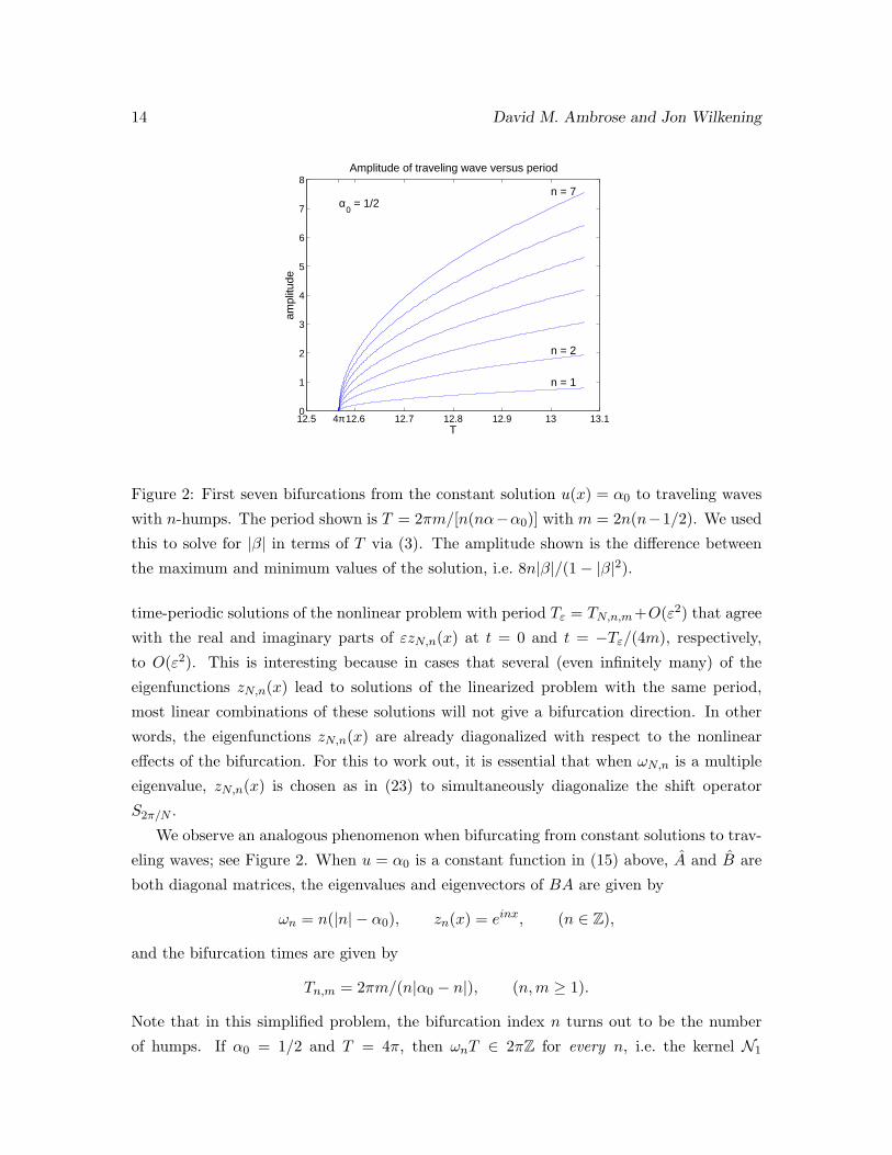
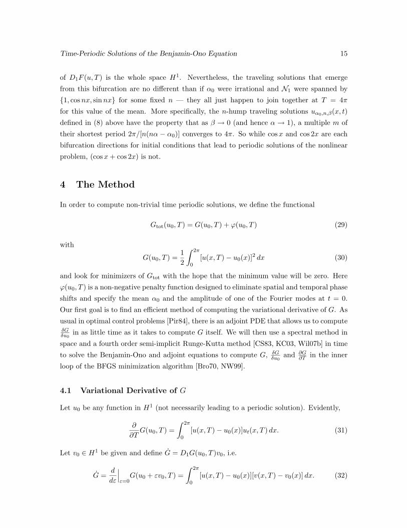
Figure 2: First seven bifurcations from the constant solution u(x) = α0 to traveling waves

with n-humps. The period shown is T = 2πm/[n(nα−α0)] with m = 2n(n−1/2). We used

this to solve for |β| in terms of T via (3). The amplitude shown is the difference between

the maximum and minimum values of the solution, i.e. 8n|β|/(1− |β|2).

time-periodic solutions of the nonlinear problem with period Tε = TN,n,m+O(ε2) that agree

with the real and imaginary parts of εzN,n(x) at t = 0 and t = −Tε/(4m), respectively,

to O(ε2). This is interesting because in cases that several (even infinitely many) of the

eigenfunctions zN,n(x) lead to solutions of the linearized problem with the same period,

most linear combinations of these solutions will not give a bifurcation direction. In other

words, the eigenfunctions zN,n(x) are already diagonalized with respect to the nonlinear

effects of the bifurcation. For this to work out, it is essential that when ωN,n is a multiple

eigenvalue, zN,n(x) is chosen as in (23) to simultaneously diagonalize the shift operator

S2π/N .

We observe an analogous phenomenon when bifurcating from constant solutions to trav-

eling waves; see Figure 2. When u = α0 is a constant function in (15) above, A and B are

both diagonal matrices, the eigenvalues and eigenvectors of BA are given by

ωn = n(|n| − α0), zn(x) = einx, (n ∈ Z),

and the bifurcation times are given by

Tn,m = 2πm/(n|α0 − n|), (n, m ≥ 1).

Note that in this simplified problem, the bifurcation index n turns out to be the number

of humps. If α0 = 1/2 and T = 4π, then ωnT ∈ 2πZ for every n, i.e. the kernel N1


of D1F (u, T ) is the whole space H1. Nevertheless, the traveling solutions that emerge

from this bifurcation are no different than if α0 were irrational and N1 were spanned by

{1, cos nx, sinnx} for some fixed n — they all just happen to join together at T = 4π

for this value of the mean. More specifically, the n-hump traveling solutions uα0,n,β(x, t)

defined in (8) above have the property that as β → 0 (and hence α → 1), a multiple m of

their shortest period 2π/[n(nα − α0)] converges to 4π. So while cos x and cos 2x are each

bifurcation directions for initial conditions that lead to periodic solutions of the nonlinear

problem, (cos x + cos 2x) is not.

4 The Method

In order to compute non-trivial time periodic solutions, we define the functional

Gtot(u0, T ) = G(u0, T ) + ϕ(u0, T ) (29)

with

G(u0, T ) =12

∫ 2π

0[u(x, T )− u0(x)]2 dx (30)

and look for minimizers of Gtot with the hope that the minimum value will be zero. Here

ϕ(u0, T ) is a non-negative penalty function designed to eliminate spatial and temporal phase

shifts and specify the mean α0 and the amplitude of one of the Fourier modes at t = 0.

Our first goal is to find an efficient method of computing the variational derivative of G. As

usual in optimal control problems [Pir84], there is an adjoint PDE that allows us to computeδGδu0

in as little time as it takes to compute G itself. We will then use a spectral method in

space and a fourth order semi-implicit Runge-Kutta method [CS83, KC03, Wil07b] in time

to solve the Benjamin-Ono and adjoint equations to compute G, δGδu0

and ∂G∂T in the inner

loop of the BFGS minimization algorithm [Bro70, NW99].

4.1 Variational Derivative of G

Let u0 be any function in H1 (not necessarily leading to a periodic solution). Evidently,

∂

∂TG(u0, T ) =

∫ 2π

0[u(x, T )− u0(x)]ut(x, T ) dx. (31)

Let v0 ∈ H1 be given and define G = D1G(u0, T )v0, i.e.

G =d

dε

∣∣∣ε=0

G(u0 + εv0, T ) =∫ 2π

0[u(x, T )− u0(x)][v(x, T )− v0(x)] dx. (32)


Here v(x, t) = u(x, t) = ddε

∣∣ε=0

u(x, t, ε) with u(x, t, ε) the solution of Benjamin-Ono with

initial condition u(x, 0, ε) = u0(x) + εv0(x). We can compute v by solving the variational

equation

vt = Hvxx − (uv)x, v(x, 0) = v0(x), (33)

which is linear but non-autonomous (as u depends on time in general). Our next task is to

eliminate v(x, T ) from (32) and represent G as an inner product:

G =∫ 2π

0

δG

δu0(x) v0(x) dx. (34)

The idea is to define a function w(x, s) going backward in time (with s = T − t) such that

w(x, 0) = w0(x) = u(x, T )− u0(x) (35)

and then determine how w should evolve so that∫ 2π

0w(x, 0)v(x, T ) dx =

∫ 2π

0w(x, T )v(x, 0) dx. (36)

Let us define the solution operator V (t2, t1) : H1 → H1 for the linearized equation (33) as

the mapping that evolves an initial condition specified at time t1 to the solution at time t2.

These operators satisfy a non-autonomous, time reversible version of familiar semigroup

properties:

V (t1, t1) = I, V (t3, t1) = V (t3, t2)V (t2, t1), (t1, t2, t3 ∈ R). (37)

Equation (36) may now be written

〈w0, V (T, 0)v0〉 = 〈W (T, 0)w0, v0〉 (38)

where 〈·, ·〉 is the L2 inner product and we define W (s2, s1) = V (t1, t2)∗ with tj = T − sj .

It follows from (37) that W (s1, s1) = I and W (s3, s1) = W (s3, s2)W (s2, s1). What remains

is to determine how this non-autonomous semigroup W is generated. Taking the inner

product of vt with w, we have∫vt(x, t)w(x, s) dx = lim

h→0

∫ ([V (t + h, t)− V (t, t)

h

]v(x, t)

)w(x, s− h) dx

= limh→0

∫v(x, t)

([W (s, s− h)− I

h

]w(x, s− h)

)dx =

∫v(x, t)ws(x, s) dx. (39)

We learn that∫vws dx =

∫vtw dx =

∫[Hvxx − (uv)x]w dx =

∫v[−Hwxx + uwx] dx, (40)


i.e. w should solve the adjoint equation to (33), namely

ws(x, s) = −Hwxx(x, s) + u(x, T − s)wx(x, s). (41)

The time reversal in the inhomogeneous term u(x, T −s) is significant. Combining this with

(32) and (34), we conclude that

δG

δu0(x) = w(x, T )− w0(x), (42)

where w solves (41) with initial condition (35).

Remark: We emphasize that the steps we have just followed for the Benjamin-Ono equation

can in principle be carried out for any PDE. These steps are simply:

1. Find the variational equation analogous to (13)

2. Find the appropriate adjoint equation, accounting for time-reversal.

The details of the initial condition of the adjoint problem and the formula for δGδu0

depend

on the particular functional G we choose, but they are usually straightforward to work out.

For example, as another variant, we could define

G(u0, T ) =12

∫ 2π

0[u(x, T/2)− u(2π − x, T/2)]2 dx (43)

to impose even symmetry at the half-way point. (Recall that if u0 is symmetric, then

u(2π − x, T/2) = u(x,−T/2)). In this case we find that

δG

δu0(x) = 2w(x, T/2), w0(x) = u(x, T/2)− u(2π − x, T/2), (44)

or, since v0 is assumed symmetric in this formulation, δGδu0

(x) = w(x, T/2)+w(2π−x, T/2).

In subsequent work, we will apply the methods of this paper to the vortex sheet with surface

tension and to the water wave. Although step 2 usually amounts to a simple integration by

parts as was done in (40) above, the adjoint calculation can be quite involved for systems of

PDEs with more complicated nonlinearities such as the Birkhoff-Rott integral in the vortex

sheet problem (see [AW09]).

4.2 The Numerical Method

We minimize Gtot using the BFGS algorithm [NW99], which is a quasi-Newton line search

method that builds an approximate Hessian incrementally from the history of gradients it

has evaluated. As a black box unconstrained minimization algorithm, it requires only an

initial guess and subroutines to compute Gtot(q) and ∇qGtot(q), where q ∈ Rd contains


the numerical degrees of freedom used to represent u0 and T . We use a solution of the

linearized problem for the initial guess near a stationary solution or traveling wave, and

then use linear extrapolation (or the result of the previous iteration) for the initial guess in

subsequent calculations as we vary the bifurcation parameter.

In our implementation, we wrote a C++ wrapper around J. Nocedal’s L-BFGS Fortran

code released in 1990, but we turn off the limited memory aspect of the code since computing

G takes more time than the linear algebra associated with updating the full Hessian matrix.

We do find that the algorithm converges quadratically once it gets close to a minimizer.

Our code also makes use of the FFTW and LAPACK libraries, but was otherwise written

from scratch.

We represent u(x, t) spectrally as a sum of M (typically 384 or 512) Fourier modes,

u(x, t) =M/2∑

k=−M/2+1

ck(t)eikx, ck ∈ C. (45)

Since u is real, we use the r2c version of the FFT algorithm, which only accesses the

coefficients ck with k ≥ 0, assuming c−k = ck. We also zero out the Nyquist frequency cM/2

so that the total number of (real) degrees of freedom representing u at time t is M − 1. We

use d = M/2 degrees of freedom to represent u0 and T , namely

q = (a0, T, a1, b1, . . . , aM/4−1, bM/4−1) ∈ Rd, (ck = ak + ibk, t = 0). (46)

The remaining Fourier modes in u0 are taken to be zero. The reason for using fewer Fourier

modes in the initial condition is that in order to avoid aliasing errors, we want the upper

half of the spectrum to remain close to zero throughout the calculation; therefore, we do

not wish to give BFGS the opportunity to modify these coefficients. We increase M and

repeat the calculation any time one of the high frequency (k ≥M/4) Fourier modes of the

optimal solution exceeds 10−13 in magnitude at any timestep.

To compute G(q), we write the Benjamin-Ono equation in the form

ut = f(u) + g(u), g(u) = Huxx, f(u) = −(

12u2)x, (47)

where 12u2 is evaluated on the grid {xj = 2πj/M : 0 ≤ j ≤M − 1} in physical space while

H and ∂x are evaluated in Fourier space. The trapezoidal rule in physical space is used

to evaluate the integral (30) defining G. To evolve the solution, we use the stiffly stable,

additive (i.e. implicit-explicit) Runge-Kutta method of Kennedy and Carpenter [KC03,

Wil07b] known as ARK4(3)6L[2]SA with a fixed timestep h = T/N , where N is chosen to

be large enough that further refinement does not improve the solution. Briefly, the idea of


an ARK method is to treat f explicitly (as it is non-linear) while treating g implicitly (as

it is the source of stiffness):

ki = f(tn + cih, un + h

∑j aijkj + h

∑j aij`j

),

`i = g(tn + cih, un + h

∑j aijkj + h

∑j aij`j

),

un+1 = un + h∑

j bjkj + h∑

j bj`j .

c A

bT

for f

c A

bT

for g

(48)

The Butcher array for f satisfies aij = 0 if i ≤ j and for g satisfies aij = 0 if i < j,

which allows the stage derivatives to be solved for in order: `1, k1, `2, k2, . . . , `6, k6, where

our scheme has 6 stages. See [KC03] for the scheme coefficients and [Wil07b] for details

on solving the implicit equations in the similar cases of Burgers’ equation and the KdV

equation.

Once u(x, T ) is known, we use the same scheme to solve the adjoint equation

ws = f(s, w) + g(w), g(w) = −Hwxx, f(s, w)(x) = u(x, T − s)wx(x). (49)

The main difficulty is that the intermediate stages of the ARK method require the value of

u at intermediate times (between timesteps). For this we use cubic Hermite interpolation,

matching u and ut at the timesteps straddling the required intermediate time:

u(·, tn + θh) = (1− θ)un + θun+1− θ(1− θ)[(1− 2θ)(un+1−un)− (1− θ)h∂tun + θh∂tun+1

]

where 0 < θ < 1. This yields fourth order accurate values of u in the right hand side of

(49), which is sufficient to achieve a fourth order accurate global solution w. We include

the option in our code to store u only at certain milemarker times, and then regenerate the

data at all timesteps between milemarkers as soon as the w equation enters that region;

this dramatically reduces the memory requirements of the code at the expense of having to

compute u twice.

Once u(x, T ) and w(x, T ) are known with the period and initial conditions specified

in q ∈ Rd, we compute G(q) using the trapezoidal rule in physical space to evaluate the

integral in (30), and we compute ∂G∂qj

by taking the FFT of δGδu0

and scaling each component


appropriately:

∂G

∂q0=∫ 2π

0

δG

δu0(x) 1 dx = 2π

(δGδu0

)∧0

∂G

∂q1=

∂G

∂T=∫ 2π

0[u(x, T )− u0(x)]ut(x, T ) dx, ←−

(use trap. rule

in physical space

)∂G

∂q2k=

∂G

∂ak=∫ 2π

0

δG

δu0(x)(eikx + e−ikx

)dx = 4π Re

{(δGδu0

)∧k

}, (k ≥ 1),

∂G

∂q2k+1=

∂G

∂bk=∫ 2π

0

δG

δu0(x)(ieikx − ie−ikx

)dx = 4π Im

{(δGδu0

)∧k

}, (k ≥ 1).

(50)

We remark that these formulas for the derivatives of the numerical version of G essentially

assume that we have solved the PDE exactly (so that the calculus of variations applies to

our numerical solutions). This is reasonable in our case as we are using spectrally accurate

schemes, but would cause difficulties if the numerical solution were only first or second order

accurate in space or time.

4.3 Choice of Penalty Function ϕ

We still need to define the penalty function ϕ(u0, T ) in (29) and show how to compute its

gradient with respect to q. The purpose of ϕ is to pin down the mean and the phase shifts

in space and time as well as to specify the bifurcation parameter. We have explored several

successful variants which became more specialized as our understanding of the problem

increased. As some of these variants may prove useful in other problems, we describe them

here.

Initially we did not include a penalty function in Gtot, but without it, the BFGS algo-

rithm invariably converges to a constant solution. Next we constrained q2, the real part of

the first Fourier mode u1(t) = a1(t) + ib1(t) at t = 0, to have a given value ρ. We reasoned

that as long as ρ is not too large, the BFGS algorithm can vary q3 = b1(0) to find a periodic

solution, so all we are doing is pinning down a phase. This was done by defining

ϕ(u0, T ) =12

([a0(0)− α0]2 + [a1(0)− ρ]2

)or ϕ(q) =

12

([q0 − α0]2 + [q2 − ρ]2

),

which works well to rule out the constant solutions but generally leads to traveling waves. By

studying these traveling waves, we determined the formulas of Section 2 and also observed

that for some choices of ρ and starting guess q(0), the wave becomes “wobbly,” indicating

that a non-trivial solution might be nearby.

To rule out traveling waves, we chose a parameter η ∈ [−1, 1] and defined

ϕ(u0, T ) =12

([a0(0)− α0]2 + [a1(0)− ρ]2 + [a1(T/2)− ηa1(0)]2 + [b1(T/2)− ηb1(0)]2

).


Our idea here was that a (one-hump) traveling wave would have η = ±1, depending on how

many times it passed through the domain in time T ; hence, intermediate values of η would

have to correspond to non-trivial solutions. To compute the gradient of ϕ when it involves

Fourier modes at later times, we simply solve another adjoint problem. Specifically, if ϕ

involves one of

ak(T/2) =12π

∫ 2π

0u(x, T/2) cos(kx) dx, bk(T/2) =

12π

∫ 2π

0u(x, T/2)[− sin(kx)] dx,

we will need to compute δδu0

ak(T/2) or δδu0

bk(T/2), which can be done by setting

w0(x) =12π

cos(kx), or w0(x) = − 12π

sin(kx)

and solving (41) from s = 0 to s = T/2; the result w(x, T/2) is the desired variational

derivative. These may then be used to compute ∂∂qj

ak(T/2) or ∂∂qj

bk(T/2) as was done for

G in (50), at which point it is a simple matter to obtain ∂ϕ∂qj

.

This procedure proved very effective in obtaining non-trivial time periodic solutions.

The BFGS algorithm is able to minimize Gtot down to 10−26, at which point roundoff

error prevents further reduction. With random initial data q(0) (which we tried before

we had solved the eigenvalue problem for the linearization), the algorithm explores quite

a wide region of the parameter space, with all components of q (including T ) changing

substantially — we do not seem to get stuck in non-zero local minima of Gtot. Once we do

find a nontrivial solution, varying η leads to other nearby periodic solutions.

Studying this family of solutions, we finally realized that we were dealing with a four

parameter family of nontrivial solutions with the mean, two phases and a bifurcation pa-

rameter describing them. The main drawback of using η as the bifurcation parameter is

that the spatial and temporal phases are not specified independently, but instead depend

on η in a complicated way. A more natural choice is to define

ϕ(u0, T ) =12

([a0(0)− α0]2 + [ak(0)− ρ]2 + [bk(0)]2 + [∂tak(0)]2

), (51)

i.e. we use ϕ to impose the mean α0, the bifurcation parameter ρ, the spatial phase bk(0) = 0,

and the temporal phase ∂tak(0) = 0. Given any solution, we can always translate space and

time to achieve the latter two conditions — we have not made any symmetry assumptions

here. The index k we use depends on the number of humps N and bifurcation index n of

the linearized solution; the only requirement is that zN,n,k in (24) be non-zero. One readily

checks that

∂tak(0) =12π

∫ 2π

0ut(x, 0) cos kx dx =

12π

∫ 2π

0

[−k2u0 + (k/2)u2

0

](− sin kx) dx, (52)


from which we obtain δδu0

[∂tak(0)](x) = 12π (k2−ku0(x)) sin kx. Although (51) does not rule

out traveling waves, we have no difficulty bifurcating from traveling waves to non-trivial

solutions by choosing a starting guess that includes first order corrections from the linear

theory of Section 3.

5 Non-Trivial Time-Periodic Solutions

We now use the methods described above to study the global behavior of non-trivial time-

periodic solutions far beyond the realm of validity of the linearization about stationary and

traveling waves. We find that these non-trivial solutions act as rungs in a ladder, connecting

stationary and traveling solutions with different speeds and wavelengths by creating or

annihilating oscillatory humps that grow or shrink in amplitude until they become part of

the stationary or traveling wave on the other side of the rung. The dynamics of these non-

trivial solutions are often very interesting, sometimes resembling a low amplitude traveling

wave superimposed on a lower frequency carrier signal, and other times behaving like two

bouncing solitons that repel each other to avoid coalescing. In this section, we present

a detailed numerical study of the path of non-trivial solutions connecting the one-hump

stationary solution to the two-hump traveling wave. In Section 6, we derive exact formulas

for the solutions on this path. In a follow-up paper [AW], we classify all bifurcations from

traveling waves, study the paths of non-trivial solutions connecting several of them, and

propose a conjecture explaining how they all fit together.

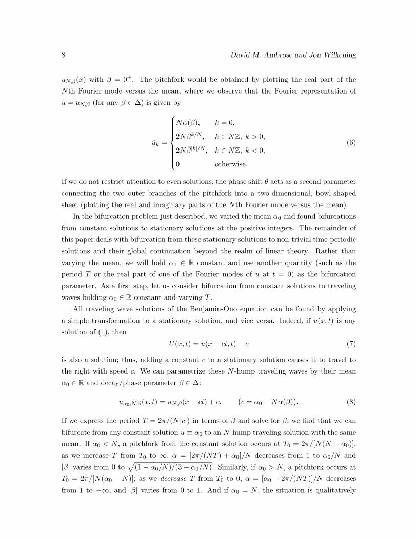
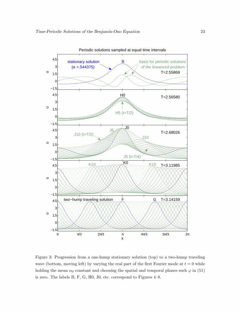
Consider the periodic solutions obtained by bifurcation from the one-hump stationary

solution at the lowest frequency, ω1,1. We arbitrarily set the mean α0 = 0.544375 for these

simulations (see Figure 1 above), but as shown in Section 6, any choice of α0 < 1 would lead

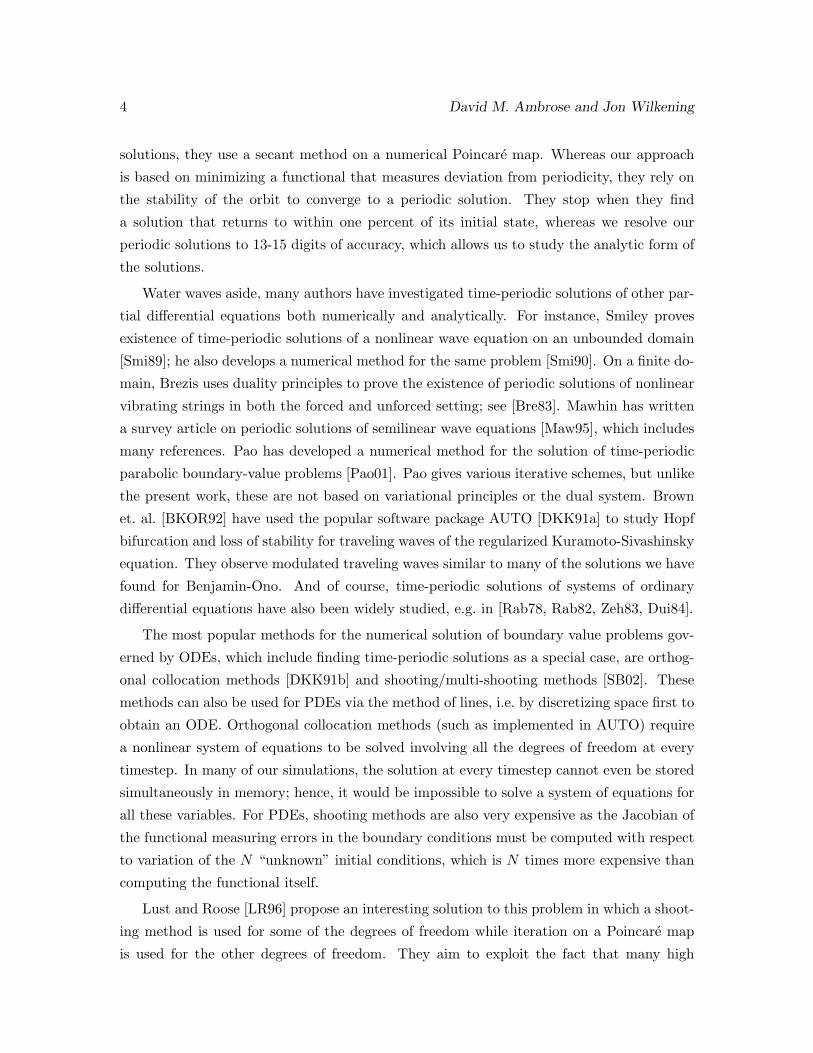
to similar results. In the top pane of Figure 3, we show the one-hump stationary solution

u1,β(x) with β = −√

(1− α0)/(3− α0) together with the (initial conditions of the) two

periodic solutions

v(0)(x, t) = Re{z1,1(x)eiω1t}, v(1)(x, t) = Im{z1,1(x)eiω1t} (53)

of the linearized equation (13) corresponding to the first eigenvalue ω1,1 = 3− α0 of BA =

−i∂x(H∂x − u). The natural period of these solutions is T = 2π/ω1,1 = 2.55869. Note how

the non-linearity of Benjamin-Ono distorts these two-hump perturbations as they travel (to

the left) on top of the one-hump stationary “carrier” solution. Also note that v(0) and v(1)

are actually the same solution with a T/4 phase lag in time:

v(0)(x, T/4) = −v(1)(x, 0) while v(1)(x, T/4) = v(0)(x, 0).


−1.5

0

1.5

3

4.5

Periodic solutions sampled at equal time intervalsu

Bstationary solution(α =.544375)

basis for periodic solutionsof the linearized problem

T=2.55869

−1.5

0

1.5

3

4.5

u

H0

H5 (t=T/2)

T=2.56580

−1.5

0

1.5

3

4.5

u

J0

J10J10 (t=T/2)

J5

J5 (t=T/4)

T=2.68026

−1.5

0

1.5

3

4.5

u

T=3.11985K0K10 K10

0 π/3 2π/3 π 4π/3 5π/3 2π−1.5

0

1.5

3

4.5

x

u

T=3.14159F Gtwo−hump traveling solution

Figure 3: Progression from a one-hump stationary solution (top) to a two-hump traveling

wave (bottom, moving left) by varying the real part of the first Fourier mode at t = 0 while

holding the mean α0 constant and choosing the spatial and temporal phases such ϕ in (51)

is zero. The labels B, F, G, H0, J0, etc. correspond to Figures 4–8.


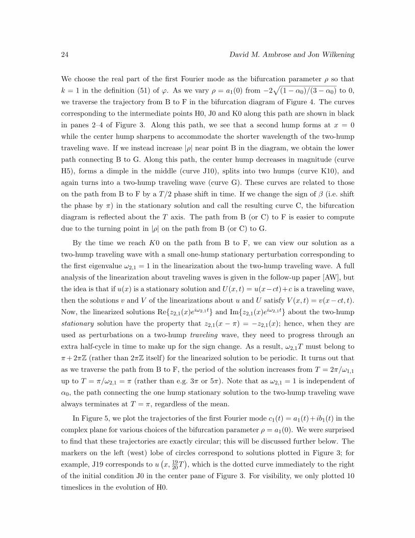
We choose the real part of the first Fourier mode as the bifurcation parameter ρ so that

k = 1 in the definition (51) of ϕ. As we vary ρ = a1(0) from −2√

(1− α0)/(3− α0) to 0,

we traverse the trajectory from B to F in the bifurcation diagram of Figure 4. The curves

corresponding to the intermediate points H0, J0 and K0 along this path are shown in black

in panes 2–4 of Figure 3. Along this path, we see that a second hump forms at x = 0

while the center hump sharpens to accommodate the shorter wavelength of the two-hump

traveling wave. If we instead increase |ρ| near point B in the diagram, we obtain the lower

path connecting B to G. Along this path, the center hump decreases in magnitude (curve

H5), forms a dimple in the middle (curve J10), splits into two humps (curve K10), and

again turns into a two-hump traveling wave (curve G). These curves are related to those

on the path from B to F by a T/2 phase shift in time. If we change the sign of β (i.e. shift

the phase by π) in the stationary solution and call the resulting curve C, the bifurcation

diagram is reflected about the T axis. The path from B (or C) to F is easier to compute

due to the turning point in |ρ| on the path from B (or C) to G.

By the time we reach K0 on the path from B to F, we can view our solution as a

two-hump traveling wave with a small one-hump stationary perturbation corresponding to

the first eigenvalue ω2,1 = 1 in the linearization about the two-hump traveling wave. A full

analysis of the linearization about traveling waves is given in the follow-up paper [AW], but

the idea is that if u(x) is a stationary solution and U(x, t) = u(x−ct)+c is a traveling wave,

then the solutions v and V of the linearizations about u and U satisfy V (x, t) = v(x− ct, t).

Now, the linearized solutions Re{z2,1(x)eiω2,1t} and Im{z2,1(x)eiω2,1t} about the two-hump

stationary solution have the property that z2,1(x − π) = −z2,1(x); hence, when they are

used as perturbations on a two-hump traveling wave, they need to progress through an

extra half-cycle in time to make up for the sign change. As a result, ω2,1T must belong to

π +2πZ (rather than 2πZ itself) for the linearized solution to be periodic. It turns out that

as we traverse the path from B to F, the period of the solution increases from T = 2π/ω1,1

up to T = π/ω2,1 = π (rather than e.g. 3π or 5π). Note that as ω2,1 = 1 is independent of

α0, the path connecting the one hump stationary solution to the two-hump traveling wave

always terminates at T = π, regardless of the mean.

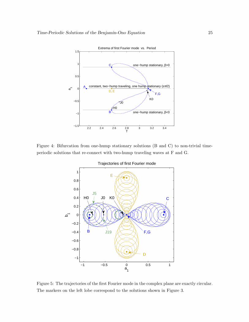
In Figure 5, we plot the trajectories of the first Fourier mode c1(t) = a1(t)+ ib1(t) in the

complex plane for various choices of the bifurcation parameter ρ = a1(0). We were surprised

to find that these trajectories are exactly circular; this will be discussed further below. The

markers on the left (west) lobe of circles correspond to solutions plotted in Figure 3; for

example, J19 corresponds to u(x, 19

20T), which is the dotted curve immediately to the right

of the initial condition J0 in the center pane of Figure 3. For visibility, we only plotted 10

timeslices in the evolution of H0.


2.2 2.4 2.6 2.8 3 3.2 3.4−1.5

−1

−0.5

0

0.5

1

1.5

A

B

C

F,GD, E

H0

J0K0

constant, two−hump traveling, one hump stationary (±π/2)

one−hump stationary, β>0

one−hump stationary, β<0

T

a 1

Extrema of first Fourier mode vs. Period

Figure 4: Bifurcation from one-hump stationary solutions (B and C) to non-trivial time-

periodic solutions that re-connect with two-hump traveling waves at F and G.

−1 −0.5 0 0.5 1

−1

−0.8

−0.6

−0.4

−0.2

0

0.2

0.4

0.6

0.8

1

Trajectories of first Fourier mode

a1

b 1

B

C

D

E

F,G

H0J5

J0

J19

K0

Figure 5: The trajectories of the first Fourier mode in the complex plane are exactly circular.

The markers on the left lobe correspond to the solutions shown in Figure 3.


The four parameter family of non-trivial solutions can be seen in Figure 5. A given

solution is represented by one of the circular trajectories. The two main parameters de-

scribing this family are the mean α0 and the distance from the nearest point on the circle

to the origin. A spatial phase shift of the initial condition by θ (with the sign convention of

Eq. (22)) amounts to a clockwise rotation of the circle about the origin by θ (or kθ for the

kth Fourier mode). The north, east and south lobes of circles represent spatial phase shifts

of the west lobe of solutions by θ = π/2, π and −π/2, respectively, but any other phase

shift θ ∈ R is also allowed. Finally, a temporal phase shift amounts to choosing which point

on the circle we assign to t = 0. Requiring that the initial condition have even symmetry

yields either the west or east lobe of solutions with t = 0 occurring along the real axis.

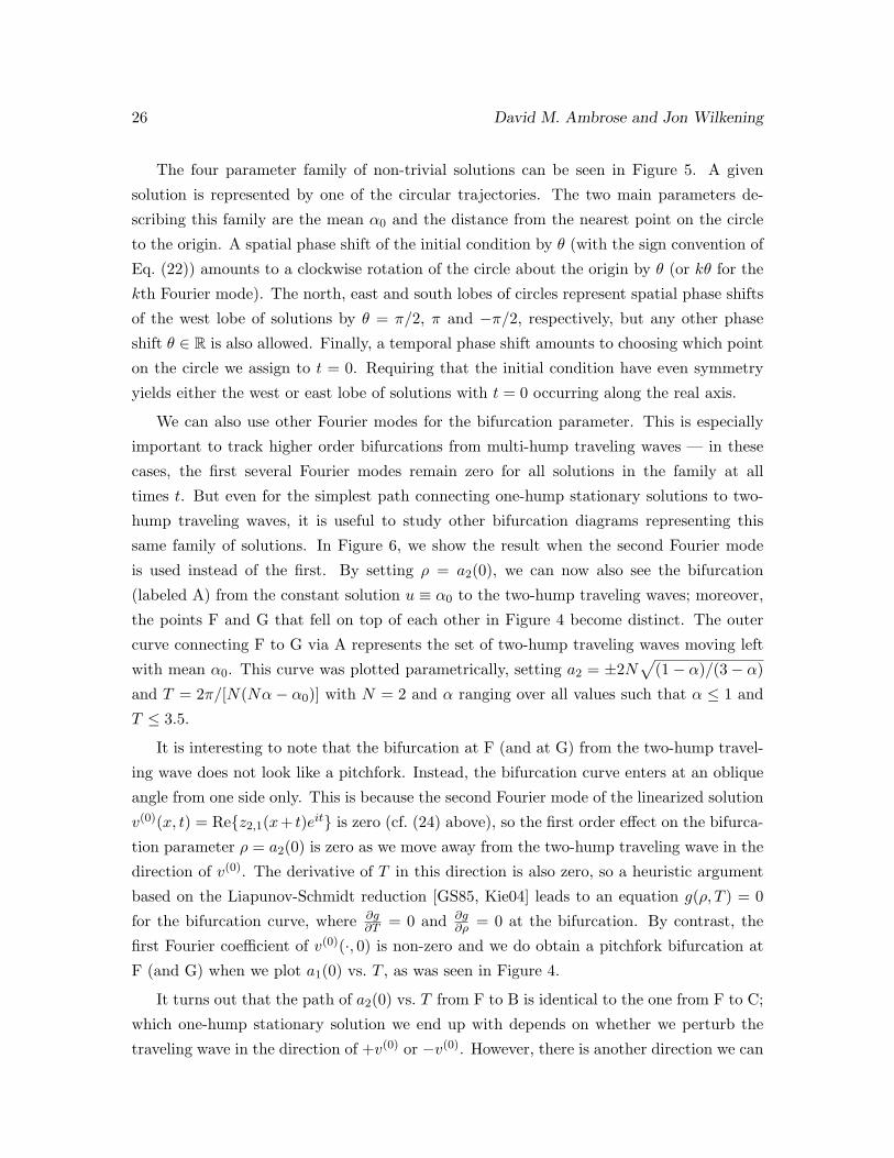
We can also use other Fourier modes for the bifurcation parameter. This is especially

important to track higher order bifurcations from multi-hump traveling waves — in these

cases, the first several Fourier modes remain zero for all solutions in the family at all

times t. But even for the simplest path connecting one-hump stationary solutions to two-

hump traveling waves, it is useful to study other bifurcation diagrams representing this

same family of solutions. In Figure 6, we show the result when the second Fourier mode

is used instead of the first. By setting ρ = a2(0), we can now also see the bifurcation

(labeled A) from the constant solution u ≡ α0 to the two-hump traveling waves; moreover,

the points F and G that fell on top of each other in Figure 4 become distinct. The outer

curve connecting F to G via A represents the set of two-hump traveling waves moving left

with mean α0. This curve was plotted parametrically, setting a2 = ±2N√

(1− α)/(3− α)

and T = 2π/[N(Nα − α0)] with N = 2 and α ranging over all values such that α ≤ 1 and

T ≤ 3.5.

It is interesting to note that the bifurcation at F (and at G) from the two-hump travel-

ing wave does not look like a pitchfork. Instead, the bifurcation curve enters at an oblique

angle from one side only. This is because the second Fourier mode of the linearized solution

v(0)(x, t) = Re{z2,1(x+ t)eit} is zero (cf. (24) above), so the first order effect on the bifurca-

tion parameter ρ = a2(0) is zero as we move away from the two-hump traveling wave in the

direction of v(0). The derivative of T in this direction is also zero, so a heuristic argument

based on the Liapunov-Schmidt reduction [GS85, Kie04] leads to an equation g(ρ, T ) = 0

for the bifurcation curve, where ∂g∂T = 0 and ∂g

∂ρ = 0 at the bifurcation. By contrast, the

first Fourier coefficient of v(0)(·, 0) is non-zero and we do obtain a pitchfork bifurcation at

F (and G) when we plot a1(0) vs. T , as was seen in Figure 4.

It turns out that the path of a2(0) vs. T from F to B is identical to the one from F to C;

which one-hump stationary solution we end up with depends on whether we perturb the

traveling wave in the direction of +v(0) or −v(0). However, there is another direction we can


2.2 2.4 2.6 2.8 3 3.2 3.4−1.5

−1

−0.5

0

0.5

1

1.5

A

B C

D E

F

G

H0

J0

K0

constant solution

one−hump stationary, ±β

one−hump stationary

(±π/2 phase shift)

two hump traveling

two hump traveling

Extrema of second Fourier mode vs. Period

T

a 2

Figure 6: Bifurcation from the constant solution to a two-hump traveling wave and the

path of non-trivial solutions connecting these to various one-hump stationary solutions.

−1.5 −1 −0.5 0 0.5 1 1.5−1.5

−1

−0.5

0

0.5

1

1.5Trajectories of second Fourier mode

a2

b 2

B,CD,E

G FK0K10 J0

K1

K2

K19

J5

H0

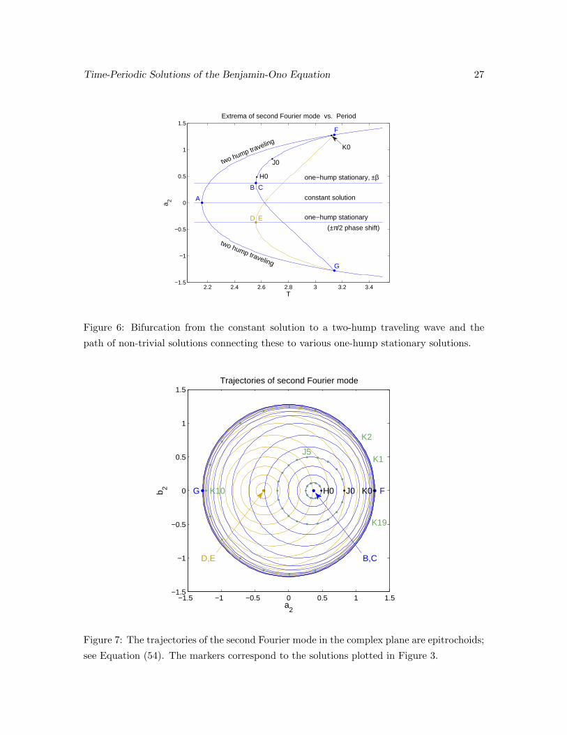
Figure 7: The trajectories of the second Fourier mode in the complex plane are epitrochoids;

see Equation (54). The markers correspond to the solutions plotted in Figure 3.


move while keeping Gtot zero (with k = 2 in (51)), namely v(1)(x, t) = Im{z2,1(x + t)eit}.This direction breaks the even symmetry of the initial condition, but the even Fourier

modes still satisfy bk(0) = 0 and ∂tak(0) = 0; hence, the penalty function ϕ does not

exclude this direction when k = 2 in (51). Depending on whether we perturb in the +v(1)

or −v(1) direction, we end up at either the one-hump stationary solution E, with maximum

at x = 3π/2, or D, with maximum at x = π/2. This shows that our choice of penalty

function ϕ in (51) does not rule out non-trivial solutions with asymmetric initial conditions:

the solutions on the path from (F or G) to (D or E) are all asymmetric at t = 0; however,

these solutions are related to the ones on the path from (F or G) to (B or C) by a phase

shift in space. We have not found any periodic solutions that cannot be made symmetric

at t = 0 by such a phase shift.

In Figure 7, we show the trajectories of the second Fourier mode in the complex plane.

The markers labeled H0, J0, etc. again correspond to the solutions plotted in Figure 3. Un-

like the first Fourier mode, these trajectories are not exactly circular — but by curve fitting

we determined they are epitrochoids, (resembling Ptolemy’s model of planetary motion, or

“spirograph” trajectories), of the form

c2(t) = c20 + c2,−1eiωt + c2,−2e

i2ωt, (ω = 2π/T ) , (54)

where the coefficients c2j (and ω) depend on the bifurcation parameter ρ. More generally,

by curve fitting our numerical solutions, we have discovered a rather amazing property of

solutions on this path: the kth Fourier mode is found to be of the form

ck(t) =0∑

j=−k

ckje−ijωt, (k ≥ 0, ω = 2π/T ), (55)

where ckj ∈ R and c−k(t) = ck(t). The general form of solutions on other paths connecting

higher order bifurcations is similar, and is described in the follow-up paper [AW]. The four

parameter family of non-trivial solutions is also nicely represented in this figure, where the

parameters are the mean, the furthest point on the epitrochoid, a global rotation about the

origin, and the choice of which point on the epitrochoid corresponds to t = 0. Note that

a spatial phase shift of the initial condition by θ leads to a rotation of a trajectory in this

figure clockwise by 2θ, so the north and south lobes of circles in Figure 5 collapse onto the

west family of epitrochoids (around D and E) in Figure 7 while the west and east lobes of

Figure 5 collapse onto the east family here.


6 Exact Solutions

The discovery that the Fourier modes execute Ptolemaic orbits of the form (55) led us to

expect that it might be possible to write down the solution in closed form. In this section,

we show how to do this for the path of non-trivial solutions connecting the one-hump

stationary solution to the two-hump traveling wave. We have now learned of several other

methods for finding exact solutions of Benjamin-Ono, notably the bilinear formalism used

by Satsuma and Ishimori [SI79] and Matsuno [Mat04] to construct multi-periodic solutions;

the reduction by Case [Cas79] of the ODE (9) to a system shown by Moser to be completely

integrable; and the approach of Dobrokhotov and Krichever [DK91] using the theory of finite

zone integration to construct multi-phase solutions. Our approach highlights a feature of

these solutions that has not been discussed previously, namely that the Fourier modes of

these solutions turn out to be power sums of particle trajectories βl(t) in the unit disk

∆ ⊂ C whose elementary symmetric functions execute simple circular orbits in the complex

plane.

We start with the observation that the meromorphic solutions

u(x, t) = α0 +N∑

l=1

uβl(t)(x), βl(t) ∈ ∆ satisfying (11), (56)

have the property that the first N + 1 Fourier modes ck(t) of u(x, t) are closely related to

the trajectories of the βl. Specifically, α0 = c0 is needed to write down the ODE (11), and

we haveβ1(t)+ · · ·+ βN (t) = s1(t), 2s1(t) = c1(t),

β21(t)+ · · ·+ β2

N (t) = s2(t), 2s2(t) = c2(t),

· · ·

βN1 (t)+ · · ·+ βN

N (t) = sN (t), 2sN (t) = cN (t).

(57)

It is a standard theorem of algebra [vdW70] that the elementary symmetric functions

σj =∑

l1<···<lj

βl1 · · ·βlj , (j = 1, . . . , N) (58)

are polynomials in the power sums, e.g.

σ0 = 1, σ1 = s1, σ2 =s21 − s2

2, σ3 =

s31 − 3s1s2 + 2s3

6. (59)

The general recurrence relation is

σ0 = 1, σj =1j

j∑l=1

(−1)l−1σj−lsl, (j = 1, . . . , N). (60)


−0.6 −0.4 −0.2 0 0.2 0.4 0.6−0.6

−0.4

−0.2

0

0.2

0.4

0.6

Particle trajectories

Re(z)

Im(z

)

B BF F

G

G

H0

J0K0

J10

J10

J12

J12

−0.5 −0.4 −0.3 −0.2 −0.1 0 0.1 0.2 0.3

−0.3

−0.2

−0.1

0

0.1

0.2

0.3

Trajectories of elementary symmetric functions

Re(z)Im

(z)

B BF

F

H0

J0

J8

J8

K0

σ1

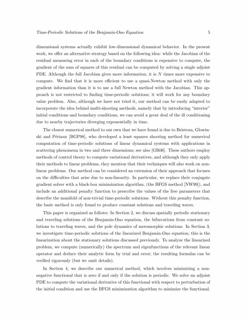
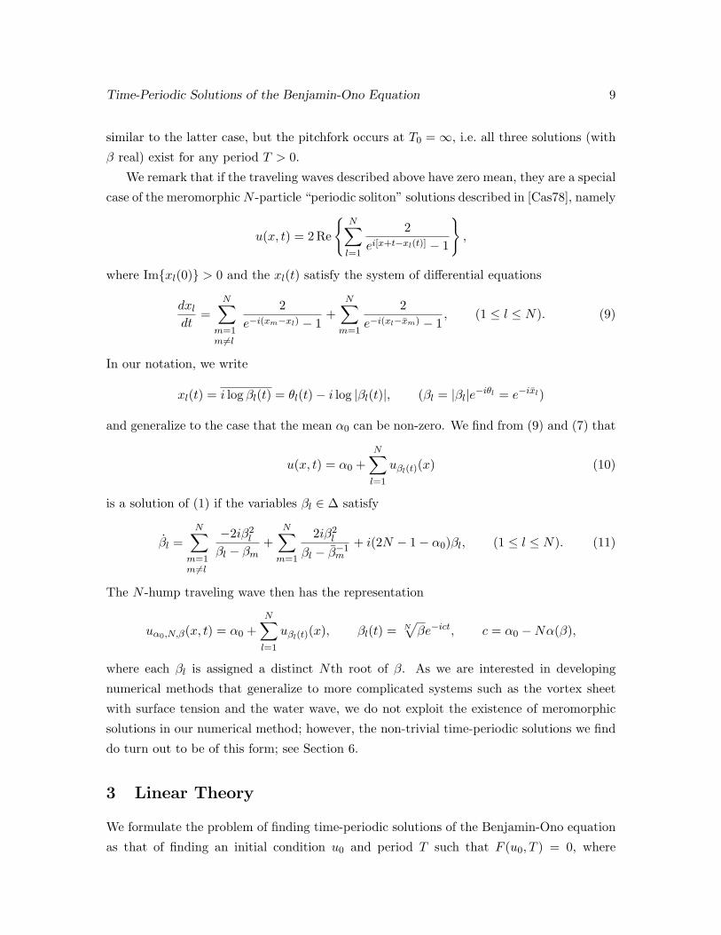
σ2

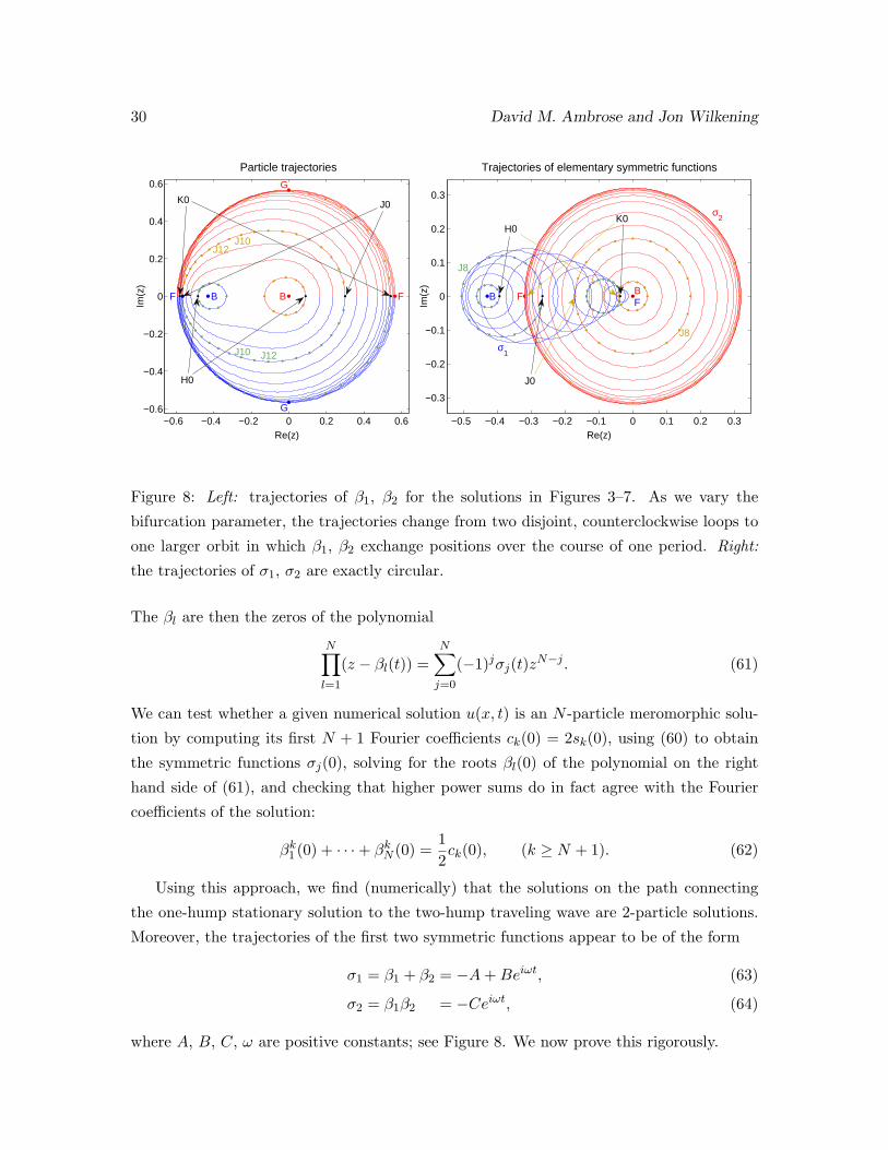
Figure 8: Left: trajectories of β1, β2 for the solutions in Figures 3–7. As we vary the

bifurcation parameter, the trajectories change from two disjoint, counterclockwise loops to

one larger orbit in which β1, β2 exchange positions over the course of one period. Right:

the trajectories of σ1, σ2 are exactly circular.

The βl are then the zeros of the polynomial

N∏l=1

(z − βl(t)) =N∑

j=0

(−1)jσj(t)zN−j . (61)

We can test whether a given numerical solution u(x, t) is an N -particle meromorphic solu-

tion by computing its first N + 1 Fourier coefficients ck(0) = 2sk(0), using (60) to obtain

the symmetric functions σj(0), solving for the roots βl(0) of the polynomial on the right

hand side of (61), and checking that higher power sums do in fact agree with the Fourier

coefficients of the solution:

βk1 (0) + · · ·+ βk

N (0) =12ck(0), (k ≥ N + 1). (62)

Using this approach, we find (numerically) that the solutions on the path connecting

the one-hump stationary solution to the two-hump traveling wave are 2-particle solutions.

Moreover, the trajectories of the first two symmetric functions appear to be of the form

σ1 = β1 + β2 = −A + Beiωt, (63)

σ2 = β1β2 = −Ceiωt, (64)

where A, B, C, ω are positive constants; see Figure 8. We now prove this rigorously.


Theorem 1 There is a four-parameter family of time-periodic, two-particle solutions of the

form

u(x, t) = α0 + uβ1(t)(x) + uβ2(t)(x), (65)

where β1(t) and β2(t) are the roots of the equation

z2 − σ1(t)z + σ2(t) = 0 (66)

and

σ1(t) = [−A + Beiω(t−t0)]e−iθ, σ2(t) = [−Ceiω(t−t0)]e−2iθ, (67)

A =(3− α0)

√[(3− α0)− (7− α0)C2

][(1− α0)− (5− α0)C2

](3− α0)2 − (5− α0)2C2

, (68)

B =5− α0

3− α0AC, (69)

ω =(3− α0)2 − (5− α0)2C2

(3− α0)− (5− α0)C2. (70)

The four parameters are the mean α0 < 1, two phases θ, t0 ∈ R, and a real number C

ranging from C = 0 (at the one-hump stationary solution) to C =√

1−α05−α0

(at the two-hump

traveling wave).

Proof: It suffices to consider the case that θ = 0 and t0 = 0 as the general case follows

immediately. If we try to substitute β1,2 = σ12 ±

12

√σ2

1 − 4σ2 into the system

β1 =−2iβ2

1

β1 − β2+

2iβ21

β1 − β−11

+2iβ2

1

β1 − β−12

+ i(3− α0)β1 (71)

β2 =−2iβ2

2

β2 − β1+

2iβ22

β2 − β−11

+2iβ2

2

β2 − β−12

+ i(3− α0)β2 (72)

and solve for A, B and ω in terms of C and α0, the algebra becomes unmanageable. However,

we can re-write this system in terms of σ1 and σ2 to obtain

σ1 = −2i

{β1(β1β1)1− β1β1

+β1(β1β2)1− β1β2

+β2(β2β1)1− β2β1

+β2(β2β2)1− β2β2

}+ i(1− α0)σ1,

σ2 = −2i

{β1β1

1− β1β1+

β1β2

1− β1β2+

β2β1

1− β2β1+

β2β2

1− β2β2

}σ2 + 2i(2− α0)σ2.

The expressions inside braces remain invariant if we interchange β1 and β2; hence, they


may be written as rational functions of σ1, σ2, σ1, σ2. Explicitly, we have

σ1 = −2iP1

Q+ i(1− α0)σ1, σ2 = −2i

P2

Qσ2 + 2i(2− α0)σ2, (73)

P1 = σ21σ1 − 2σ1σ2 − 2σ3

1σ2 + 6σ1|σ2|2 − σ1σ21σ2 + 2σ2

1σ1|σ2|2 − 2σ1σ22σ2 − 2σ1|σ2|4,

P2 = |σ1|2(1 + 3|σ2|2

)+ 4|σ2|2

(1− |σ2|2

)− 2(σ2

1σ2 + σ21σ2

),

Q =(1− |σ2|2

)2 − |σ1|2(1 + |σ2|2

)+(σ2

1σ2 + σ21σ2

).

Since Q is a product of non-zero terms of the form (1−βiβj), it is never zero. If we assume

σ1 = −A + Beiωt, σ2 = −Ceiωt, and C 6= 0, we find that (73) holds as long as[− 2P1 + (1− α0)σ1Q

]+

B

C

[− 2P2σ2 + (4− 2α0)σ2Q

]= 0, (74)

−2P2 + (4− 2α0 − ω)Q = 0. (75)

We eliminated ω in (74) using σ1 = iωBeiωt = −BC σ2. Next, we collect terms containing

like powers of eiωt and set them each to zero. This yields 7 polynomial equations in the

variables A, B, C, α0 and ω; however, several of them are redundant due to relationships

such as Q(−1) = Q(1) in the decomposition Q = Q(−1)e−iωt + Q(0) + Q(1)eiωt. Equation

(74) yields 4 such equations; two of them are satisfied if we choose B as in (69) while the

remaining two are satisfied if we also choose A as in (68). With these choices, all three

equations associated with (75) are satisfied provided ω satisfies (70). The special cases

{C = 0, A =√

1−α03−α0

, B = 0} and {C =√

1−α05−α0

, A = 0, B = 0} are seen to correspond to

the one-hump stationary solution and two-hump traveling wave, respectively, as discussed

in Section 2.

We have verified that the curve connecting B to F in the bifurcation diagram of Figure 4

is recovered if we set α0 = .544375 and plot 2(−A + B) versus T = 2π/ω using the above

formulas for A, B and ω with C ranging from 0 to√

1−α05−α0

.

7 Conclusion

We have presented a general method for finding continua of time-periodic solutions for

nonlinear systems of partial differential equations. We have used our method to study global

paths of non-trivial time-periodic solutions connecting stationary and traveling waves of the

Benjamin-Ono equation. In spite of the non-linearity and non-locality of the Benjamin-Ono

equation, these non-trivial solutions can be interpreted as distorted superpositions of the

stationary or traveling waves at each end of the path. Our numerical method is accurate

enough that we are able to use data fitting techniques to recognize the analytical form of


the solutions. In particular, the Fourier coefficients ck(t) of these solutions follow Ptolemaic

orbits of the form (55). This led us to reformulate the equations governing meromorphic

pole dynamics to reveal an exact formula for the solutions on the four-parameter path

connecting the one-hump stationary solution to the two-hump traveling wave.

In the future, we plan to apply this method to more complicated systems arising in fluid

dynamics, namely the vortex sheet and water wave problems. This will allow for comparison

with prior numerical and analytical results [HLS97], [PT01], [IPT05]. Additionally, as the

Benjamin-Ono equation is meant as a model for internal waves in a deep, stratified fluid,

it will be of interest to compare time-periodic vortex sheets and water waves with time-

periodic solutions of Benjamin-Ono.

References

[Are63] R. F. Arenstorf. Periodic solutions of the restricted three body problem rep-

resenting analytic continuations of Keplerian elliptic motions. Amer. J. Math.,

LXXXV:27–35, 1963.

[AW] D. M. Ambrose and J. Wilkening. Global paths of time-periodic solutions of

the Benjamin-Ono equation connecting pairs of traveling waves. Comm. App.

Math. and Comp. Sci. (accepted).

[AW09] D. M. Ambrose and J. Wilkening. Computation of time-periodic solutions of

the vortex sheet with surface tension. 2009. (in preparation).

[Ben67] T. B. Benjamin. Internal waves of permanent form in fluids of great depth. J.

Fluid Mech., 29(3):559–592, 1967.

[BGP98] M. O. Bristeau, R. Glowinski, and J. Periaux. Controllability methods for the

computation of time-periodic solutions; application to scattering. J. Comput.

Phys., 147:265–292, 1998.

[BKOR92] H. S. Brown, I. G. Kevrekidis, A. Oron, and P. Rosenau. Bifurcations and

pattern formation in the “regularized” Kuramoto-Sivashinsky equation. Physics

Letters A, 163:299–308, 1992.

[Bre83] H. Brezis. Periodic solutions of nonlinear vibrating strings and duality principles.

Bull. Amer. Math. Soc. (N.S.), 8:409–426, 1983.

[Bro70] C. G. Broyden. The convergence of a class of double-rank minimization algo-

rithms, Parts I and II. J. Inst Maths Applics, 6:76–90, 222–231, 1970.


[Cas78] K. M. Case. The N-soliton solution of the Benjamin–Ono equation. Proc. Natl.

Acad. Sci. USA, 75(8):3562–3563, 1978.

[Cas79] K. M. Case. Meromorphic solutions of the Benjamin–Ono equation. Physica,

96A:173–182, 1979.

[CI05] M. Chen and G. Iooss. Standing waves for a two-way model system for water

waves. European J. Mech. B/Fluids, 24:113–124, 2005.

[CR04] M. Cabral and R. Rosa. Chaos for a damped and forced KdV equation. Physica

D, 192:265–278, 2004.

[Cra96] A. Crannell. The existence of many periodic non-travelling solutions to the

Boussinesq equation. J. Differential Equations, 126:169–183, 1996.

[CS83] G. J. Cooper and A. Sayfy. Additive Runge-Kutta methods for stiff ordinary

differential equations. Math. Comp., 40(161):207–218, 1983.

[DA67] R.E. Davis and A. Acrivos. Solitary internal waves in deep fluid. J. Fluid Mech.,

29:593–607, 1967.

[DK91] S. Yu. Dobrokhotov and I. M. Krichever. Multi-phase solutions of the Benjamin-

Ono equation and their averaging. Math. Notes, 49:583–594, 1991.

[DKK91a] E. J. Doedel, H. B. Keller, and J. P. Kernevez. Numerical analysis and control

of bifurcation problems: (I) Bifurcation in finite dimensions. Int. J. Bifurcation

and Chaos, 1(3):493–520, 1991.

[DKK91b] E. J. Doedel, H. B. Keller, and J. P. Kernevez. Numerical analysis and control of

bifurcation problems: (II) Bifurcation in infinite dimensions. Int. J. Bifurcation

and Chaos, 1(4):745–772, 1991.

[Dui84] J. J. Duistermaat. Bifurcations of periodic solutions near equilibrium points of

Hamiltonian systems. In Bifurcation Theory and Applications, volume 1057 of

Lecture Notes in Mathematics, pages 57–105. Springer, Berlin, 1984.

[FB85] Richard J. Field and Maria Burger. Oscillations and Traveling Waves in Chem-

ical Systems. John Wiley and Sons, New York, 1985.

[Gov00] Willy J. F. Govaerts. Numerical Methods for Bifurcations of Dynamical Equi-

libria. SIAM, Philadelphia, 2000.


[GR06] R. Glowinski and T. Rossi. A mixed formulation and exact controllability ap-

proach for the computation of the periodic solutions of the scalar wave equation.

(I): Controllability problem formulation and related iterative solution. C. R.

Acad. Sci. Paris, Ser. I, 343:493–498, 2006.

[GS85] Martin Golubitsky and David G. Schaeffer. Singularities and Groups in Bifur-

cation Theory, volume I and II. Springer-Verlag, New York, 1985.

[GV91] J. Ginibre and G. Velo. Smoothing properties and existence of solutions for

the generalized Benjamin-Ono equations. J. Differential Equation, 93:150–212,

1991.

[HLS94] T. Hou, J. Lowengrub, and M. Shelley. Removing the stiffness from interfacial

flows with surface tension. J. Comput. Phys., 114(2):312–338, 1994.

[HLS97] T. Hou, J. Lowengrub, and M. Shelley. The long-time motion of vortex sheets

with surface tension. Phys. Fluids, 9(7):1933–1954, 1997.

[HNW00] Ernst Hairer, Syvert P. Norsett, and Gerhard Wanner. Solving Ordinary Dif-

ferential Equations I: Nonstiff Problems. Springer, Berlin, 2nd edition, 2000.

[IPT05] G. Iooss, P.I. Plotnikov, and J.F. Toland. Standing waves on an infinitely deep

perfect fluid under gravity. Arch. Rat. Mech. Anal., 177:367–478, 2005.

[KC03] C. A. Kennedy and M. H. Carpenter. Additive Runge-Kutta schemes for

convection-diffusion-reaction equations. Appl. Numer. Math., 44(1–2):139–181,

2003.

[Kie04] Hansjorg Kielhofer. Bifurcation Theory: An Introduction with Applications to

PDEs. Springer, New York, 2004.

[LR96] K. Lust and D. Roose. Newton-Picard methods with subspace iteration for com-

puting periodic solutions of partial differential equations. ZAMM, 76(S2):605–

606, 1996.

[Mat04] Y. Matsuno. New representations of multiperiodic and multisoliton solutions

for a class of nonlocal soliton equations. J. Phys. Soc. Jpn., 73(12):3285–3293,

2004.

[Maw95] J. Mawhin. Periodic solutions of some semilinear wave equations and systems:

A survey. Chaos, Solitons & Fractals, pages 1651–1669, 1995.


[Nir01] Louis Nirenberg. Topics in Nonlinear Functional Analysis. American Mathe-

matical Society, Providence, 2001.

[NW99] Jorge Nocedal and Stephen J. Wright. Numerical Optimization. Springer, New

York, 1999.

[Ono75] H. Ono. Algebraic solitary waves in stratified fluids. J. Phys. Soc. Japan,

39:1082–1091, 1975.

[Pao01] C.V. Pao. Numerical methods for time-periodic solutions of nonlinear parabolic

boundary value problems. SIAM J. Numer. Anal., pages 647–667, 2001.

[Pir84] O. Pironeau. Optimal Shape Design for Elliptic Systems. springer-Verlag, New

York, 1984.

[PT01] P.I. Plotnikov and J.F. Toland. Nash-Moser theory for standing water waves.

Arch. Rat. Mech. Anal., 159:1–83, 2001.

[Rab78] P. H. Rabinowitz. Periodic solutions of Hamiltonian systems. Comm. Pure Appl.

Math., 31:157–184, 1978.

[Rab82] P. H. Rabinowitz. Periodic solutions of Hamiltonian systems: A survey. SIAM

J. Math. Anal., 13:343–352, 1982.

[Sau79] J.C. Saut. Sur quelques generalisations de l’equation de Korteweg-deVries. J.

Math. Pures Appl., 58:21–61, 1979.

[SB02] J. Stoer and R. Bulirsch. Introduction to Numerical Analysis. Springer, New

York, third edition, 2002.

[SI79] J. Satsuma and Y. Ishimori. Periodic wave and rational soliton solutions of the

Benjamin-Ono equation. J. Phys. Soc. Jpn., 46(2):681–687, 1979.

[Smi89] M.W. Smiley. Breathers and forced oscillations of nonlinear wave equations on

R3. J. Reine Angew. Math., 398:25–35, 1989.

[Smi90] M.W. Smiley. Numerical determination of breathers and forced oscillations of

nonlinear wave equations. In Computational solution of nonlinear system of

equations, volume 26 of Lectures in Appl. Math., pages 605–617, Providence,

RI, 1990. American Mathematical Society.

[Str00] Steven H. Strogatz. Nonlinear Dynamics and Chaos. Perseus Books Group,

2000.


[Tao04] T. Tao. Global well-posedness for the Benjamin-Ono equation in H1(R). J.

Hyperbolic Diff. Eq., 1:27–49, 2004.

[vdW70] B. L. van der Waerden. Algebra, volume 1. Unger, New York, 1970.

[Wil07a] J. Wilkening. An algorithm for computing Jordan chains and inverting analytic

matrix functions. Linear Algebra Appl., 427:6–25, 2007.

[Wil07b] Jon Wilkening. Math 228A Lecture Notes: Numerical Solution of Differential

Equations. UC Berkeley, 2007. Available from author’s webpage.

[Zeh83] E. Zehnder. Periodic solutions of Hamiltonian equations. In Dynamics and Pro-

cesses, volume 1031 of Lecture Notes in Mathematics, pages 172–213. Springer,

Berlin, 1983.

Documents

Computation of Time-Periodic Solutions of the Benjamin-Ono