Competitive Prices and Organizational Choices∗

Patrick Legros† and Andrew F. Newman‡

April 2008

Abstract

We construct a price-theoretic model of integration decisions and show that

these choices may adversely affect consumers, even in the absence of monopoly

power in supply and product markets. Integration is costly to implement but

is effective at coordinating production decisions. The price of output helps

to determine the organizational form chosen: there is an inverted-U relation

between the degree of integration and product prices. Moreover, organizational

choices affect output: integration is more productive than non-integration at

low prices, and less productive at high prices. Since shocks to industries affect

product prices, reorganizations are likely to take place in coordinated fashion

and be industry specific, consistent with the evidence. Since the price range

in which integration maximizes productivity generally differs from the one in

which it maximizes managerial welfare, organizational choices will often be

second-best inefficient. We show that there are instances in which entry of

low-cost suppliers can hurt consumers by changing the terms of trade in the

supplier market, thereby inducing reorganizations that raise prices.

∗Preliminary. Some of the material in this paper circulated in as earlier paper circulated underthe title “ Managerial Firms, Organizational Choice, and Consumer Welfare.” We thank RolandBenabou, Patrick Bolton, Phil Bond, Estelle Cantillon, Paola Conconi, Jay Pil Choi, Mathias De-watripont, Robert Gibbons, Oliver Hart, Georg Kirchsteiger, Giovanni Maggi, Armin Schmuckler,and George Symeonidis for helpful discussion. Legros benefited from the financial support of theCommunaute Francaise de Belgique (projects ARC 98/03-221 and ARC00/05-252), and EU TMRNetwork contract noFMRX-CT98-0203. Newman was the Richard B. Fisher Member of the Institutefor Advanced Study, Princeton when some of the research for this paper was conducted.†ECARES, Universite Libre de Bruxelles, and CEPR.‡Boston University and CEPR.

1 Introduction

Do consumers have an interest in the internal organization of the firms that make the

products they buy? Conventional economic wisdom says no, at least if product mar-

kets are characterized by a reasonable degree of competition: firms that fail to deliver

the goods at the lowest feasible cost, whatever the reason, including inappropriate

organization, will be supplanted by their more efficient competitors.1

There are, of course, potential interest conflicts between the firm and the con-

sumer: this is a central concern of the industrial organization literature and of com-

petition policy. But the predominant model of the firm there is the classical one of

the unitary profit maximizer; as a consequence, the effects of organizational design on

market performance are generally absent from the analysis, and both the economic

literature and policy practice have focused instead on the adverse effects of market

power. In this context, mergers or other major reorganizations are worthy of concern

only insofar as they increase the firm’s market power. In particular, it would be hard

from this point of view to see how firms might be characterized by too little integra-

tion, something for which there is at least some evidence (Bertrand and Mullainathan,

2003).

Addressing the still-open question of whether organizational decisions can affect

consumer welfare in ways that do not involve market power requires adopting a richer

model of the firm, one which views organizational decisions as the purview of man-

agers who trade off the usual pecuniary costs and benefits, such as profits, with

noncontractible ones such as managerial effort, working conditions, corporate cul-

ture, or leadership vision. This is the perspective that predominates in the modern

theory of the firm (Grossman and Hart 1986; Hart and Moore 1990).

This literature has consistently emphasized how, in environments with imperfect

or incomplete contracting, managerial firms may make organizational decisions that

have little to do with profit maximization and/or the interests of owners. In this paper

we will show that similar inefficiencies are likely to arise from the consumer point

of view. Organizational design is influenced by product prices, because they affect

the terms of managerial trade-offs. At the same time, organizational choice affects

prices because it determines productivity. Even in a competitive world, inefficiencies

are likely to be significant: both too much and too little integration are possible

outcomes.

1For instance, as Fama and Jensen (1983) aver, “the form of organization that survives... is theone that delivers the product demanded by customers at the lowest price while covering costs.”

1

To keep things simple, we rule out market foreclosure effects altogether by as-

suming competitive product and supplier markets. Production of consumer goods

requires the combination of exactly two complementary suppliers, each consisting of

a manager and his collections of assets.2 When the suppliers form a joint enterprise

(or “firm”), the managers operate the assets by taking noncontractible decisions.

As in some of the more recent models of firms, in particular Hart and Holm-

strom (2002), the production technology essentially involves the adoption of stan-

dards. While there is no objectively “right” decision, output is higher on average the

more decisions are in the same direction. The problem is that managers disagree about

which direction they ought to go. This may reflect differences in background (engi-

neering favors elegant design; sales prefers user-friendliness and redundant features),

information (a content provider may want to broadcast mass-market programming,

while the local distributor thinks programs must be specifically tailored to a local

market), or technology (the BTU and sulphur content of coal needs to be optimally

adapted to a power plant’s boiler and emissions equipment). Each party will find it

costly to accommodate the other’s approach, but if they don’t agree on something,

the market will be poorly served.

Under non-integration, managers make their decisions separately, and this may

lead to inefficient production. Integration solves this problem by bringing in an addi-

tional party, called HQ, which is motivated by monetary compensation to maximize

the enterprise’s output.3 HQ accomplishes this by enforcing a common standard. But

delegating decision rights to HQ does not come for free, and generates two types of

losses. First this solution to the coordination problem may lead to high private costs

for the initial managers. Second, using HQ to enforce coordination may have direct

costs in terms of foregone output. For instance, HQ may lack expertise in the tasks

carried out by the suppliers, (e.g., Hart and Moore 1999), there may be additional

communication and delay costs (e.g., Radner 1993, Bolton and Dewatripont 1994),

or HQ may have its own moral hazard problems.

Whether to integrate is decided by managers when the firms form; this takes place

in a competitive supplier market in which the two types of suppliers “match”. The

firms’ output is sold in a competitive product market, wherein all firms and consumers

2The model is inspired by earlier work (Legros and Newman 1996, forthcoming) that shows howcompetitive market conditions determine organizational design such as the degree of monitoring orthe allocation of control. Those papers do not consider the interaction of organization with theproduct market or consumer welfare, however.

3Other models that take this view of integration include Alchian and Demsetz (1972), Hart andHolmstrom (2002), Mailath et al. (2002).

2

are price-takers.

At low prices, managers do not value the increase in output brought by integration

since they are not compensated sufficiently for the high costs they have to bear. At

very high prices, managers value output so much that they are willing to concede in

order to achieve coordination. Therefore integration only emerges for intermediate

levels of price. In other words, there is an inverted U-shaped relationship between

product price and the degree of integration.

A convenient feature of the model is that the derivation of equilibrium organiza-

tional choices and product prices reduces to a standard supply-and-demand analysis,

where the industry supply curve embodies the price-dependent organizational deci-

sions described above. We apply this framework to show how internal organization,

as well as prices and quantities, respond to shocks such as changes in product de-

mand or entry of additional suppliers. Incorporating organizational design into this

otherwise standard analysis can lead to surprising results: for instance we identify

regimes where product prices increase and consumer welfare decreases following pos-

itive shocks, such as the entry of low-cost suppliers.

The price mechanism also provides a natural explanation for the tendency for

organizational restructuring to be widespread. There is considerable evidence that

firms integrate (or divest) in “waves” and that reorganizations of this sort are most

pronounced at the industry level. Since product price is common to a whole industry,

anything that changes it will not only have the classical price-theoretic quantity and

consumer welfare effects, but will have organizational effects as well. And as we have

suggested, these organizational effects will in turn feed back to quantity and welfare.

A consumer welfare criterion would favor output-enhancing organizations, and

there is a simple characterization of the prices at which the managers’ organizational

choices fail this measure. If we use a total-surplus criterion, weighing consumer and

firm surpluses equally, the inefficiency persists as long as managers are not full residual

claimants. This begs the question of whether outside owners can discipline managers

into taking the profit maximizing organizational decision. We show that instruments

such as variable profit shares, free cash flow, even imposing the integration decision

directly, will not eliminate the inefficiencies – and in some cases make things worse.

2 Model

There are two types of supplier, denoted A and B. To produce a unit of marketable

output requires the coordinated input of one A and one B, and we call their union

3

a firm. Examples of A and B might include game consoles and game software, up-

stream and downstream enterprises, or manufacturing and customer support. For

each provider, a decision is rendered indicating the way in which production is to

be carried out. For instance software can be elegant or user friendly, or a product

line and its associated marketing campaign can be mass- or niche-market oriented.

Denote the decision in an A supplier by a ∈ [0, 1], and a B decision by b ∈ [0, 1]. It

is important that decisions made in each part of the firm do not conflict, else there is

loss of output. More precisely, the enterprise will succeed with a probability equal to

1− (a− b)2, in which case it generates a unit of output; otherwise it fails, yielding 0.

Overseeing each provider is a risk-neutral manager, who bears a private cost of

the decision made in his unit. The managers’ payoffs are increasing in income, but

they disagree about the direction decisions ought to go: what is easy for one is hard

for the other, and vice versa. Specifically, we assume that the A manager’s utility is

yA − (1− a)2, and the B manager’s utility is yB − b2, where yA ≥ 0 and yB ≥ 0 are

the respective realized incomes.4

Decisions are not contractible, but the managers have two contractual instruments

with which to resolve their interest conflicts. First, the firm’s revenue is contractible,

allowing for the provision of monetary incentives via sharing rules. Second, the right to

make decisions can be contractually assigned. Here there are two options. Managers

can remain non-integrated, in which case they retain control over their respective deci-

sions. Alternatively, they can can integrate by engaging the service of a headquarters

(HQ).

HQ is empowered to decide both a and b, and is motivated only by monetary

concerns, incurring no direct cost from the decisions. Using HQ does impose a (social)

cost that we model as a reduction σ ≥ 0 in the expected output. One interpretation is

that this arise from a moral hazard problem: given its considerable decision power, HQ

may be able to divert resources into other activities, including private benefits, other

ventures, or pet projects.5 Alternatively, σ arises from added costs of communication,

additional personnel, or the use of decision makers who are less specialized than the

4Although we model the managers disagreement as differences in preferences, we expect verysimilar results could be generated by a model in which they differ in “vision” as in van den Steen(2005).

5For instance, suppose that after output is realized, there is a probability σ that HQ has a chanceto divert whatever output there is to an alternative use valued at ν times its market value, whereσ < ν < 1. If output is diverted, it doesn’t reach the market, and the verifiable information is thesame as if the firm had failed. Managers could prevent diversion by offering a share ν to HQ, leaving(1 − ν) of the revenue to be shared between the managers, but since ν > σ, it is actually betterfor them to give HQ a zero share of market revenue and let him divert when he is able, so thatsuccessfully produced output reaches consumers only (1− σ) of the time.

4

A and B managers. In this case, HQ gets a fixed share of the revenue, with σ being

(approximately) the sum of the output loss and HQ’s share.6

Regardless of who determines a and b, managers bear the cost, because they have

to “live with the decision”: their primary function is to implement them and to

convince their workforces to agree.7

To summarize, expected output is (1 − (a − b)2)(1 − σI), where I, denoting the

ownership structure, is equal to one if the firm is integrated and zero if it is not.

Before production, B managers match with A managers in the supplier market,

signing contracts (s, I), that specify the ownership structure I and the share s ∈ [0, 1]

of managerial revenue accruing to the manager of A, with 1 − s accruing to the B

(note that both receive zero in case of failure).

There is a competitive product market. Firms take the (correctly anticipated)

price P as given when they sign contracts and take their decisions. The demand side

of the product market is modeled as a decreasing demand function D(P ).

In the supplier market, there is a continuum of both types of suppliers. The

A’s are on the long side of the market: their measure is n > 1, while the B’s have

unit measure. All unmatched A managers receive an outside option payoff uA, which

except in Section 3.2 we take to be zero (the outside option of B-managers will play

little role here and can be taken to be 0).8

For now we take the total managerial revenue in case of success to be the product

market price P .

2.1 Integration

With integration, HQ receives an expected surplus proportional to (1 − (a − b)2)P

and therefore chooses a = b, which maximizes the firm’s expected revenue. Among

all a = b choices, the one that minimizes the total cost is a = 1/2, and we assume

that HQ will choose these decisions (indeed, as the managers’ payoffs are perfectly

transferable by varying the share s, this choice is Pareto optimal among the firm’s

6There is a small difference between the interpretation in that in the first case, the reduction inoutput and the reduction in revenue perceived by the managers are identical, whereas in the lattercase, these differ by the amount of HQ’s share; no substantial difference in any of our conclusionswould arise if we were to take explicit account of this distinction.

7Logically speaking, there is an alternative form of integration which does without HQ, insteaddelegating full control to one of the managers, who will subsequently perfectly coordinate the deci-sions in his preferred direction. It is straightforward to show (section 2.2) that this form of integrationis dominated by the other forms in this model.

8In fact it is a simple matter to generalize the model to the case of non zero and even heterogeneousoutside options all around; see section 7.1 in the Appendix.

5

decision makers). The cost to each manager is then 14, and the payoffs to the A and

B managers are

uIA(s, P ) = (1− σ)sP − 1

4

uIB(s, P ) = (1− σ)(1− s)P − 1

4.

Total managerial welfare under integration is W I(P ) = (1−σ)P − 12

and, as we have

noted, is fully transferable.

2.2 Non-integration

Since each manager retains control of his activity, given a share s, A chooses a ∈ [0, 1] ,

B chooses b ∈ [0, 1] as the (unique) Nash equilibrium of a game with payoffs

uNA = (1− (a− b)2)sP − (1− a)2

uNB = (1− (a− b)2)(1− s)P − b2.

These choices are:

aN =1 + (1− s)P

1 + P(1)

bN =(1− s)P

1 + P, (2)

and the resulting expected output is

QN(P ) = 1− 1

(1 + P )2(3)

which is independent of s. Output is increasing in the price P : a higher product

price raises the relative importance of the revenue motive against private costs,and

this pushes the managers to better coordinate.

Of course, the managers’ payoffs depend on s; they are:

uNA (s, P ) = QN(P )sP − s2

(P

1 + P

)2

(4)

uNB (s, P ) = QN(P )(1− s)P − (1− s)2

(P

1 + P

)2

. (5)

Varying s, one obtains the Pareto frontier for non-integration. It is straightforward

6

to verify that it is strictly concave and that the total managerial payoff WN(s, P ) =

QN(P )P − (s2 + (1− s)2)(

P1+P

)2is maximized at s = 1/2 and minimized at s = 0 or

s = 1. Note that when s = 0, a = 1: the A manager makes no concession, and only

the B bears a positive private cost.9

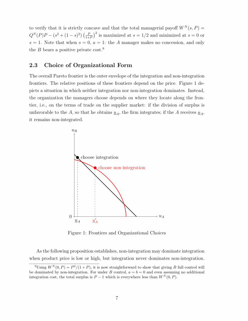
2.3 Choice of Organizational Form

The overall Pareto frontier is the outer envelope of the integration and non-integration

frontiers. The relative positions of these frontiers depend on the price. Figure 1 de-

picts a situation in which neither integration nor non-integration dominates. Instead,

the organization the managers choose depends on where they locate along the fron-

tier, i.e., on the terms of trade on the supplier market: if the division of surplus is

unfavorable to the A, so that he obtains uA, the firm integrates; if the A receives uA,

it remains non-integrated.

0 uA

uB

choose integration

choose non-integration

u′AuA

Figure 1: Frontiers and Organizational Choices

As the following proposition establishes, non-integration may dominate integration

when product price is low or high, but integration never dominates non-integration.

9Using WN (0, P ) = P 2/(1 +P ), it is now straightforward to show that giving B full control willbe dominated by non-integration. For under B control, a = b = 0 and even assuming no additionalintegration cost, the total surplus is P − 1 which is everywhere less than WN (0, P ).

7

There is a range of prices where integration is preferred to non-integration when B’s

share of surplus is large enough.

Proposition 1 When σ is positive, managerial welfare with integration

(i) is smaller than the minimum total welfare with non-integration if and only if P

does not belong to the interval [π, π] , where π and π are the two solutions of the

equation σ = P−12P (1+P )

.

(ii) is smaller than the maximum welfare with non-integration.

It is straightforward to see that [π, π] is nonempty only when σ is weakly smaller

than a positive upper bound σ, that π is increasing and π is decreasing in σ, and that

π becomes unbounded as σ → 0.

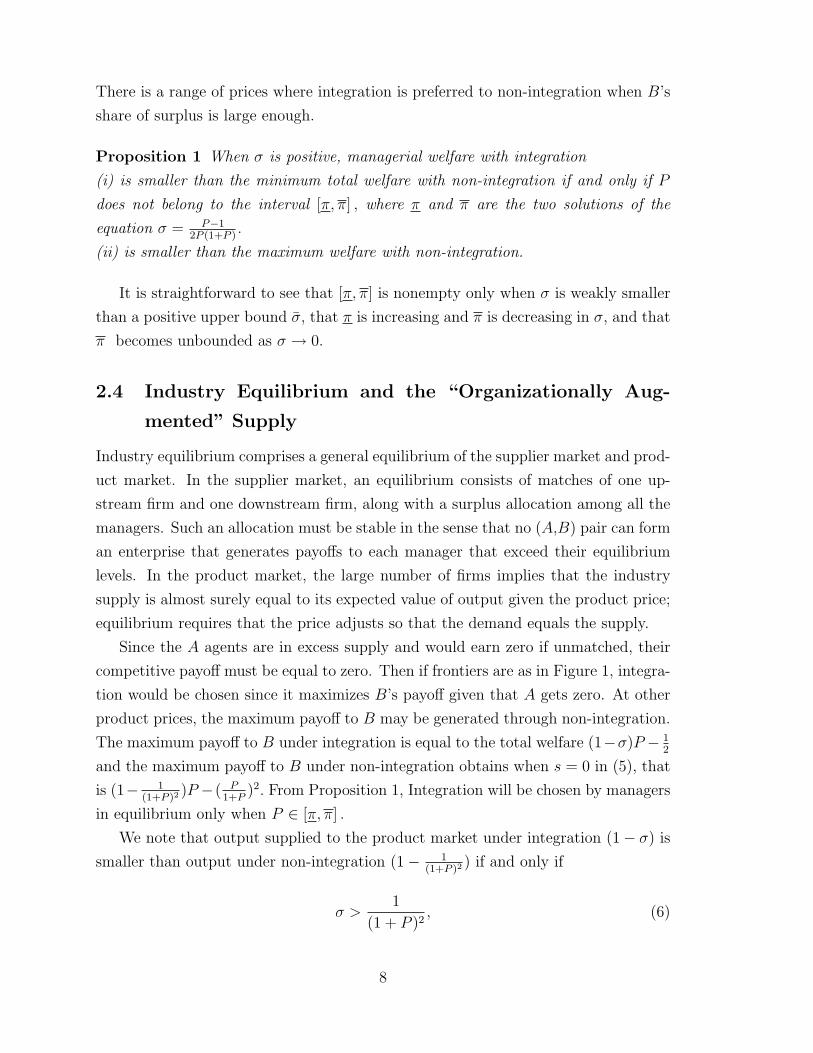
2.4 Industry Equilibrium and the “Organizationally Aug-

mented” Supply

Industry equilibrium comprises a general equilibrium of the supplier market and prod-

uct market. In the supplier market, an equilibrium consists of matches of one up-

stream firm and one downstream firm, along with a surplus allocation among all the

managers. Such an allocation must be stable in the sense that no (A,B) pair can form

an enterprise that generates payoffs to each manager that exceed their equilibrium

levels. In the product market, the large number of firms implies that the industry

supply is almost surely equal to its expected value of output given the product price;

equilibrium requires that the price adjusts so that the demand equals the supply.

Since the A agents are in excess supply and would earn zero if unmatched, their

competitive payoff must be equal to zero. Then if frontiers are as in Figure 1, integra-

tion would be chosen since it maximizes B’s payoff given that A gets zero. At other

product prices, the maximum payoff to B may be generated through non-integration.

The maximum payoff to B under integration is equal to the total welfare (1−σ)P − 12

and the maximum payoff to B under non-integration obtains when s = 0 in (5), that

is (1− 1(1+P )2

)P −( P1+P

)2. From Proposition 1, Integration will be chosen by managers

in equilibrium only when P ∈ [π, π] .

We note that output supplied to the product market under integration (1− σ) is

smaller than output under non-integration (1− 1(1+P )2

) if and only if

σ >1

(1 + P )2, (6)

8

that is when

P > π∗(σ) =

√1

σ− 1. (7)

It is straightforward to see that π∗ ∈ (π, π) whenever σ < σ.

The reason non-integration generates higher output as price increases is simple

enough: the higher is P, the more revenue figures in managers’ payoffs. This leads

one to “ concede” to the other’s decision in order to reduce output losses.

The non-monotonicity of managers’ organizational preference in price when σ ∈(0, σ) is more subtle. At low prices, despite integration’s better output performance,

revenue is still small enough that the managers (in particular the manager of B)

are more concerned with their private benefits, i.e., they like the quiet life. At high

prices, non-integration performs well enough in the output dimension that they do

not want to incur the cost σ of HQ. Only for intermediate prices do managers prefer

integration. In this range, the B manager knows that revenue is large enough that

he will be induced to bear a large private cost to match the perfectly self indulgent

A manager, who generates little income from the firm (s = 0) and therefore chooses

a = 1. B prefers the relatively high output and moderate private cost that he incurs

under integration.10

As mentioned earlier, the demand side of the product market is represented by

the demand function D(P ). To derive industry supply, suppose that a fraction α of

firms are integrated and a fraction 1− α are non-integrated. Total supply at price P

is then

S(P, α) = α(1− σ) + (1− α)

(1−

(1

1 + P

)2). (8)

For σ < σ, when P < π, α = 0 and total supply is just the output when all firms

choose non-integration. At P = π, α can vary between 0 and 1 since managers are

indifferent between the two forms of organization; however because π < π∗, output

is greater with integration and as α increases total supply increases. When α = 1

output is 1 − σ and stays at this level for all P ∈ (π, π). At P = π, managers are

10 For this outcome, it is crucial that the supplier market be “unbalanced,” i.e., that A or Bbe accruing the preponderance of the surplus. For as we already noted, the total surplus undernon-integration when it is equally shared (s = 1/2) always exceeds that generated by integration.Thus if surplus is (nearly) equally shared by A and B, (for instance, if one side has a nonzero outsideoption), they never integrate. On the other hand, our specific functional forms are not critical tothis kind of outcome: similar results obtain if the managers have a standard partnership problem,where total net revenue is Pf(a, b) and the non-contractible cost functions CA(a) and CB(b) areincreasing in a and b. Details are in section 7.7 in the Appendix.

9

again indifferent between the two ownership structures and α can decrease from 1 to

0 continuously; because π∗ < π, output is greater the smaller is α. Finally for P > π

all firms remain non-integrated and output increases with P.

When σ ≥ σ, managers always choose non-integration and α = 0 for all prices.

We therefore write S(P, α(P )) to represent the supply correspondence, where α(P )

is described in the previous paragraph. The supply curve for the case σ ∈ (0, σ) is

represented in Figure 2. The dotted curve corresponds to the industry supply when

no firms are integrated.

0 Q

P

1− σ

π∗(σ)

π(σ)

π(σ)

N

M

I

M

N

Figure 2: Organizationally Augmented Supply Curve (No Outside Options, σ < σ)

An equilibrium in the product market is a price and a quantity that equate supply

and demand: D(P ) ∈ S(P, α(P )). There are three distinct types of industry equilib-

ria, depending on where along the supply curve the equilibrium price occurs: those

in which firms integrate (I), the mixed equilibria in which some firms integrate and

others do not (M), and a pure non-integration equilibrium (N).

The product market supply embodies organization choices by managers. The

model suggests that industries in which product prices are high or low will be pre-

dominately composed of non-integrated firms, while those with intermediate prices

will tend to be integrated. The model is also useful for illuminating sources of changes

in organization.

10

3 Comparative Statics

The fact that all firms face the same price means that anything that affects that price

– a demand shift or foreign competition – can lead to widespread and simultaneous

reorganization, e.g., a merger wave or mass divestiture. An additional channel of

coordinated reorganization is the supplier market: changes in the relative scarcities

of the two sides, or to outside opportunities on one side, will change the way surplus is

divided between managers, and this too will lead to reorganization.11 In some cases

these changes in the supplier market terms of trade will have surprising effects on

product market outcomes.

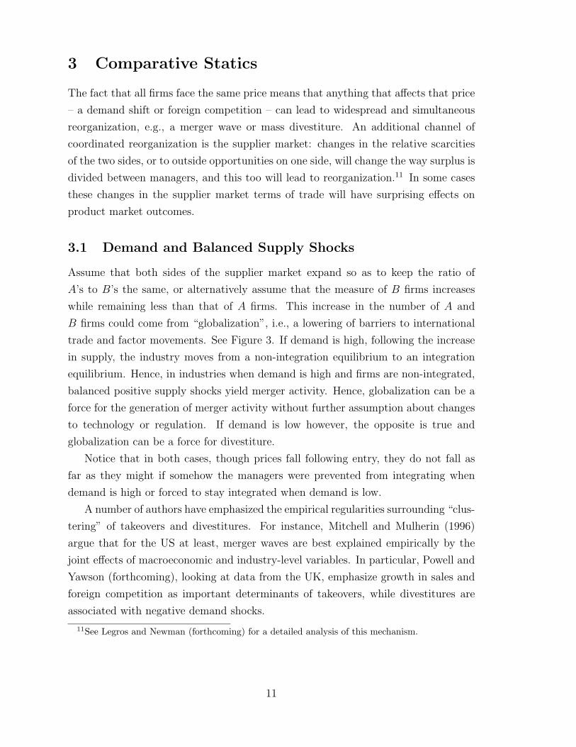
3.1 Demand and Balanced Supply Shocks

Assume that both sides of the supplier market expand so as to keep the ratio of

A’s to B’s the same, or alternatively assume that the measure of B firms increases

while remaining less than that of A firms. This increase in the number of A and

B firms could come from “globalization”, i.e., a lowering of barriers to international

trade and factor movements. See Figure 3. If demand is high, following the increase

in supply, the industry moves from a non-integration equilibrium to an integration

equilibrium. Hence, in industries when demand is high and firms are non-integrated,

balanced positive supply shocks yield merger activity. Hence, globalization can be a

force for the generation of merger activity without further assumption about changes

to technology or regulation. If demand is low however, the opposite is true and

globalization can be a force for divestiture.

Notice that in both cases, though prices fall following entry, they do not fall as

far as they might if somehow the managers were prevented from integrating when

demand is high or forced to stay integrated when demand is low.

A number of authors have emphasized the empirical regularities surrounding “clus-

tering” of takeovers and divestitures. For instance, Mitchell and Mulherin (1996)

argue that for the US at least, merger waves are best explained empirically by the

joint effects of macroeconomic and industry-level variables. In particular, Powell and

Yawson (forthcoming), looking at data from the UK, emphasize growth in sales and

foreign competition as important determinants of takeovers, while divestitures are

associated with negative demand shocks.

11See Legros and Newman (forthcoming) for a detailed analysis of this mechanism.

11

Q

π

1− σ m(1− σ)

π∗

π

π

move to integration

move to non-integration

Figure 3: Positive Supply Shock

3.2 Entry of Low Cost Suppliers

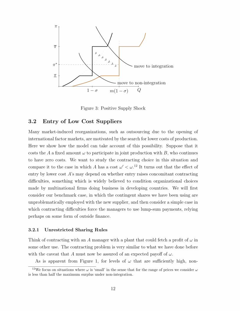
Many market-induced reorganizations, such as outsourcing due to the opening of

international factor markets, are motivated by the search for lower costs of production.

Here we show how the model can take account of this possibility. Suppose that it

costs the A a fixed amount ω to participate in joint production with B, who continues

to have zero costs. We want to study the contracting choice in this situation and

compare it to the case in which A has a cost ω′ < ω.12 It turns out that the effect of

entry by lower cost A’s may depend on whether entry raises concomitant contracting

difficulties, something which is widely believed to condition organizational choices

made by multinational firms doing business in developing countries. We will first

consider our benchmark case, in which the contingent shares we have been using are

unproblematically employed with the new supplier, and then consider a simple case in

which contracting difficulties force the managers to use lump-sum payments, relying

perhaps on some form of outside finance.

3.2.1 Unrestricted Sharing Rules

Think of contracting with an A manager with a plant that could fetch a profit of ω in

some other use. The contracting problem is very similar to what we have done before

with the caveat that A must now be assured of an expected payoff of ω.

As is apparent from Figure 1, for levels of ω that are sufficiently high, non-

12We focus on situations where ω is ‘small’ in the sense that for the range of prices we consider ωis less than half the maximum surplus under non-integration.

12

Q

P

Figure 4: Entry of lower cost suppliers: Contingent Shares

integration will be chosen. As A’s opportunity cost decreases, it becomes feasible

(and optimal) for the B to integrate with A. Hence, if at price P integration is op-

timal at cost ω, it will be also be optimal for any ω′ < ω; because the preference is

strict at ω′ when there is indifference at ω, there are more prices for which integration

is preferred under ω′. Thus, if sharing rules are employed, reduced costs are a force

toward integration. This is represented in the Figure 4.

Of particular interest when low-cost suppliers enter the market is whether the

resulting cost savings are passed on to consumers in the form of lower prices. As

shown in the figure, this need not be the case: if prices are initially moderately high,

the reorganization used to accomodate the changing terms of trade in the supplier

market lead to a reduction in output and an increase in prices. When demand is low,

though, entry of low-cost A’s yields the the usual comparative static of lower prices

and higher quantities.

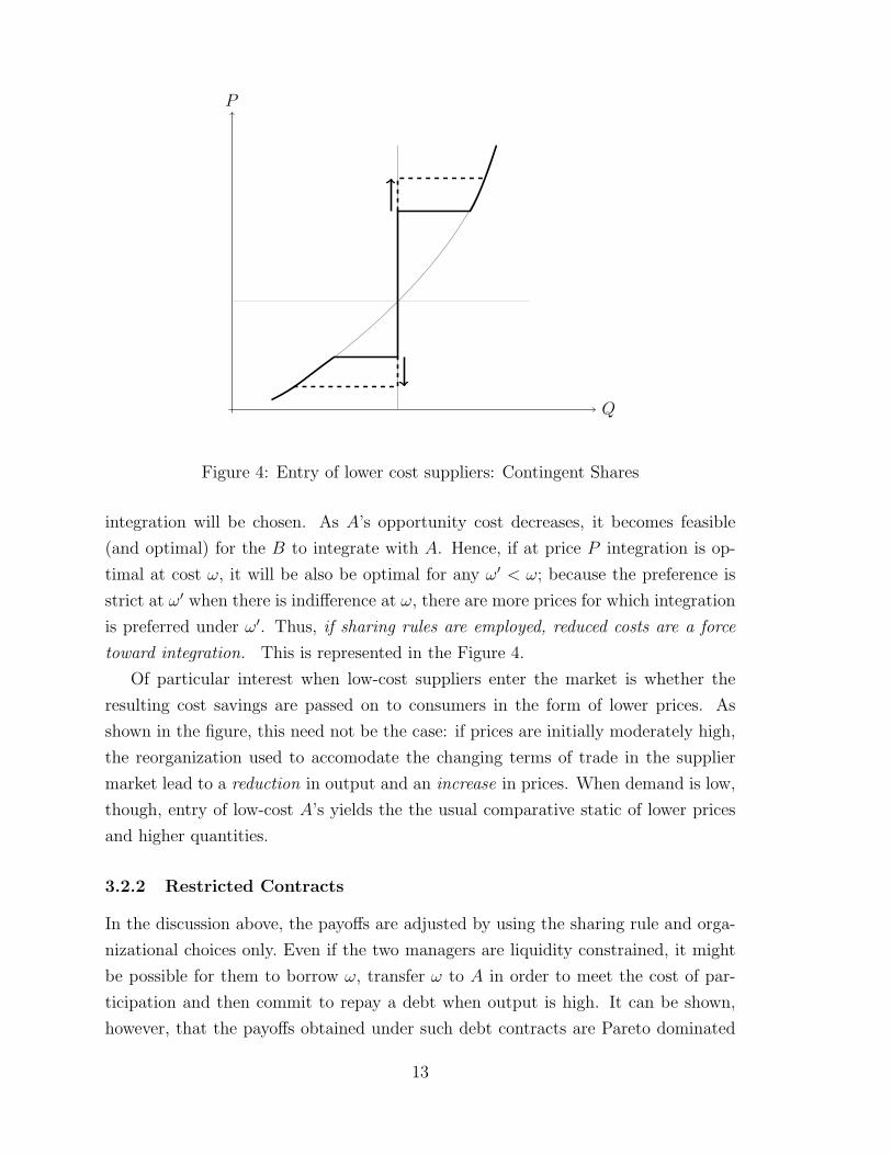
3.2.2 Restricted Contracts

In the discussion above, the payoffs are adjusted by using the sharing rule and orga-

nizational choices only. Even if the two managers are liquidity constrained, it might

be possible for them to borrow ω, transfer ω to A in order to meet the cost of par-

ticipation and then commit to repay a debt when output is high. It can be shown,

however, that the payoffs obtained under such debt contracts are Pareto dominated

13

by contracts without debt, and will therefore never be used if sharing rules are avail-

able.13

Nevertheless, it is worth considering what happens if sharing rules are problematic,

say because of the “contracting difficulties” that are often thought to account for ver-

tical integration (especially FDI) of multinational firms with suppliers in developing

countries.

We model this in a simple way, by supposing that s ≡ 0, so that ω must be paid

up front. Moreover, we assume that B does not have enough cash for this, so that the

firm will need to borrow ω from the financial market in exchange for a state contingent

debt repayment D in case of success and 0 in case of failure. The market for loans

is competitive. Under integration, the level of price does not affect the probability of

success and the probability of repayment is one; the B manager’s surplus is therefore

uIB(P, ω) = (1− σ)P − 1/2− ω, as in the previous case.

Under non-integration however, debt distorts B’s incentives to concede. He faces

an effective price of P − D; since for low P the success probability will tend to be

small, D will be large, so that the distortion is especially large at low prices. Now, if B

was indifferent between integration and non-integration, he will favor non-integration

after a decrease in ω. This is true not only at high prices, where the result is a

downward shift in the supply curve, but also at low prices, where the resulting gain

of efficiency of non-integration relative to integration enlarges the set of prices at

which it is preferred. Details are shown in the Appendix.14

With restricted contracts, then, lower costs are a force away from integration.

Alternatively the interval [π(σ), π(σ)] over which integration is preferred to non-

integration is decreasing in ω (that is the lower bound increases and the upper bound

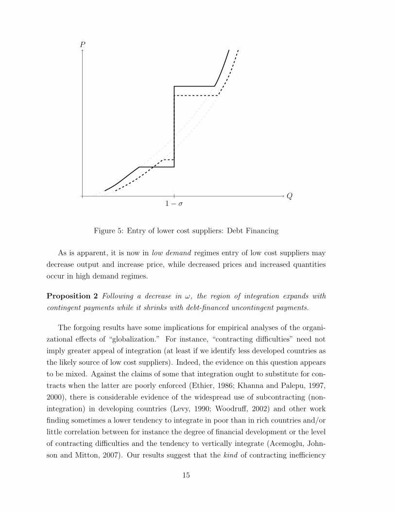
decreases). This leads to a shift of the industry supply as in Figure 5.

13The reason is that under non-integration, debt distorts the incentives of the borrower, since itreduces his effective share of output, while the fixed payment is sunk and therefore does nothing toimprove the incentives of the recipient; if instead an equivalent reduction in the borrower’s share isused to increase the recipient’s share, then the borrower’s incentive reduction is at least partiallyoffset by stronger incentives for the recipient. Under integration, debt has no impact on efficiency.See Legros and Newman (forthcoming).

14Note that the debt has the effect of lowering the price perceived by the managers. For thisreason it may be tempting to view the effect of debt as that of a per-unit tax: for a given priceP and a level of debt D the organizational choice should be the same under price P − D and nodebt. This reasoning would imply that both the lower bound π and the upper bound π increase.But this intuition is incorrect because it does not take into account the different incentive effectsthat debt on different organizations. In particular, because the lender needs to recover ω, the “tax”rate is large at low prices and small at high ones under non-integration; hence the distortion is largeat low prices, leading firms to prefer (undistorted) integration at prices at which they would prefernon-integration in the absence of the tax.

14

Q

P

1− σ

Figure 5: Entry of lower cost suppliers: Debt Financing

As is apparent, it is now in low demand regimes entry of low cost suppliers may

decrease output and increase price, while decreased prices and increased quantities

occur in high demand regimes.

Proposition 2 Following a decrease in ω, the region of integration expands with

contingent payments while it shrinks with debt-financed uncontingent payments.

The forgoing results have some implications for empirical analyses of the organi-

zational effects of “globalization.” For instance, “contracting difficulties” need not

imply greater appeal of integration (at least if we identify less developed countries as

the likely source of low cost suppliers). Indeed, the evidence on this question appears

to be mixed. Against the claims of some that integration ought to substitute for con-

tracts when the latter are poorly enforced (Ethier, 1986; Khanna and Palepu, 1997,

2000), there is considerable evidence of the widespread use of subcontracting (non-

integration) in developing countries (Levy, 1990; Woodruff, 2002) and other work

finding sometimes a lower tendency to integrate in poor than in rich countries and/or

little correlation between for instance the degree of financial development or the level

of contracting difficulties and the tendency to vertically integrate (Acemoglu, John-

son and Mitton, 2007). Our results suggest that the kind of contracting inefficiency

15

(e.g. the ease of implementing sharing rules vs the ease of procuring outside finance),

as well as the differential effects of financial distortions across organizational types,

may be crucial for determining whether integration or non-integration is likely to be

attractive in poor countries.

Relatedly, empirical assessments of the effects of globalization on organizational

choice as well as on prices and quantities may need to take account of the sources of

lower costs and the ways these can be accommodated contractually across national

borders. Models such as this one signal that the issues cannot be ignored if there is

to be any hope of drawing clear lessons from the evidence.

4 Welfare

Welfare analysis is straightforward if we use a consumer welfare criterion: in this

case, we know that managers choose inefficiently integration when their revenue π is

in the interval (π∗, π) and choose inefficiently non-integration when their revenue is

less than π. It follows that as long as the welfare criterion puts enough weight on

consumer surplus, the equilibrium choice of organization will be inefficient for some

regions of prices.

However, a consumer welfare criterion puts no emphasis on managerial costs and

this begs the question of whether integration decisions can be second-best inefficient

when managerial costs are taken into consideration. Below, we use a total welfare

measure, that is the sum of consumer and firm (owners and managers) welfare. For a

given demand function, we compare the equilibrium welfare to the welfare that would

be generated if the equilibrium form of organization is not allowed. For instance,

we will say that an equilibrium with integration is second-best efficient if welfare is

greater than in the equilibrium where firms are forced to choose non-integration.

Since the firm surplus incorporates managerial costs, it is convenient to express

the managerial cost as a function of the expected quantity produced by the firm.

When there is integration, this cost is equal to 1/4. Consider now non-integration,

and assume that the A suppliers have a zero outside option; in equilibrium their share

will be equal to zero and they do not bear a cost since a = 1. Suppose that manager

B chooses decision b; then output is Q(1, b) and total managerial cost is CB(b). Now,

since Q(1, b) = Q has a unique solution (b = 1−√

1−Q), we can write the managerial

cost as a function of Q only:

c(Q) = CB(b(Q))

16

For manager B, the solution to maxb πQ(1, b)−CB(b) is then the same as the solution

to maxQ πQ− c(Q). It follows that along the graph (π,Q(π)), we have π = c′(Q(π)):

when the manager faces revenue π, expected output equates π to the marginal man-

agerial cost.

Equipped with this observation, we can now illustrates the cases where equilibria

are second-best inefficient. Until now we have assumed that the managerial revenue

in case of success is equal to P . This will be the case if the managers are full residual

claimant for the revenue. In general one expects the managers to get only a share

of the revenue, and for simplicity we will assume in this section that for any price P

managers have a revenue π(P ) = λP where λ is less than one. We also focus on the

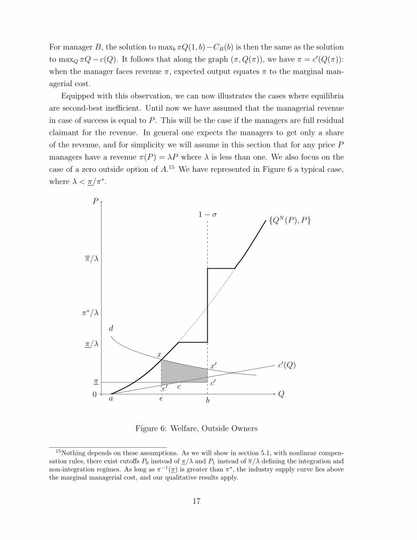
case of a zero outside option of A.15 We have represented in Figure 6 a typical case,

where λ < π/π∗.

0 Q

P

b

1− σ

a

{QN(P ), P}

π∗/λ

π/λ

π/λ

d

x

x′

π c′

c′(Q)

e

ce′

Figure 6: Welfare, Outside Owners

15Nothing depends on these assumptions. As we will show in section 5.1, with nonlinear compen-sation rules, there exist cutoffs P0 instead of π/λ and P1 instead of π/λ defining the integration andnon-integration regimes. As long as π−1(π) is greater than π∗, the industry supply curve lies abovethe marginal managerial cost, and our qualitative results apply.

17

The supply curve under non-integration is QN(P ) = 1 − 1/[(1 + λP ))2]. Hence,

in the supply-demand diagram, the marginal cost curve coincides with the curve

(QN(λP ), λP ), and is strictly below the supply curve, as illustrated in Figure 6.

Hence, moving from integration to non-integration will generate a social gain when

P ∈ (π∗/λ, π/λ) and as long as the demand is sufficiently elastic the equilibrium will

be second-best inefficient. Intuitively, the gain in output is first order now while the

increase in managerial costs is second order.

By the same argument, an industry equilibrium at P ∈ [0, P/λ] can also be second-

best inefficient. Indeed, in this range of prices, since managerial costs are a smaller

part of total welfare, the large gain in welfare obtained by consumers and owners

when moving from non-integration to integration in the case P < π/λ may dominate

the managerial loss. The equilibrium may therefore be second-best inefficient for low

levels of output.

For the demand d, equilibrium is at x and welfare is the area d− x− e′ − a since

the managerial cost is the triangle a − e′ − e. If integration is forced, the industry

equilibrium would be at x′ with welfare equal to d−x′− c′− c−a. There is therefore

a deadweight loss equal to the area x− x′ − c− e′.16

Note that if the demand is more inelastic, the deadweight loss is lower. Under

weak conditions, it is possible to characterize the region of inefficient non-integration.

A family of demand functions {Q = d(P ; t), t ∈ R+} is regular if for each P and t,

d(P, t) is strictly increasing in t, strictly decreasing in P , limP→0 d(P, t) = ∞, and

for each Q and t there exists P such that d(P, t) = Q. Hence, in a regular family,

demand functions do not intersect the horizontal axis, two demand functions do not

intersect and demand functions are onto R+.

Proposition 3 Suppose λ < π/π∗. Consider a regular family of demand functions.

Then, there exist equilibrium prices Pm ∈ (0, π/λ] and PM ∈ (π∗/λ, π/λ) correspond-

ing to two demand functions in this family such that for any other demand function

in the family:

(i) if the equilibrium specifies integration, it is second-best efficient only if P ≤ PM ,

and

(ii) if the equilibrium specifies non-integration, it is second-best efficient if and only

if P ≤ Pm.

16Since at the revenue level π, managers are indifferent between integration and non-integration,we must have QN (π)π−c(QN (π)) = (1−σ)QN (π)−1/2, and it follows that the cost under integrationof 1/4 is equal to the area a− c− c′ − b− a.

18

This proposition shows that firms are characterized by too little and too much

integration from a total welfare point of view. As λ = 1, when managers are full

residual claimants, we show in the Appendix that equilibria are second-best efficient.

5 Control by Outside Owners

In our competitive world, when the managers are not full residual claimants, outside

owners have nearly the same interests as consumers: they value output enhancing

organizations. Corporate control by outside owners may therefore mitigate the inef-

ficiencies we have identified in the previous section. We will consider two types of

instruments that owners may use. First, we will allow the owners to design price

contingent revenues π(P ) for the managers. Second, we will consider the possibility

for owners to give managers cash in order to make the surplus under non-integration

more transferable. We will show that in both cases, second-best inefficiencies persist:

in the first case because owners partially internalize the managerial costs, in the sec-

ond case because managers will favor non-integration more and therefore the region

of prices for which non-integration is second-best inefficient is larger.

5.1 Price Contingent Compensation

We assume here that owners can choose managerial shares π(P ) that are contingent

on the market price P . We will consider first the situation where managers are

delegated the right to decide integration or non-integration. We will then analyze the

case where the owners have full control on the organization.

5.1.1 Managers Choose the Organization

Suppose that owners want the managers to choose integration: the cheapest way for

them to do so is to give a fixed compensation in case of success of π (or ε greater than

this to avoid indifference). Hence, the maximum payoff to owners when they want to

implement integration is

vI(P ) = (1− σ)(P − π)

Suppose now that the owners want to implement non-integration. They are con-

strained in their choice since they need to choose π that is not in the interval [π, π]. Let

us, however, ignore the constraint for the moment. The value under non-integration

19

is given by the function vN(P ),

vN(P ) = maxπ≥0

(1− 1

(1 + π)2

)(P − π) (9)

Lemma 4 The solution π∗ to (9) is a strictly convex and strictly increasing function

of P . It follows that there exists unique price levels P , P such that π∗(P ) = π and

π∗(P ) = π.

Proof. The objective is strictly concave in π and strictly supermodular in (π, P ) , so

that the (unique) optimum π(P ) is increasing in P . Consequently, QN(π(P )) is also

increasing, and there exist unique values of prices P , P ∗, and P such that π = π(P ),

π∗ = π (P ∗), and π = π(P ). Since by the envelope theorem vN ′(P ) = QN(π(P )),

vN(P ) is (strictly) convex.

Convexity of vN , linearity of vI and the fact that for prices less than 1 integration

leads to a negative payoff while non-integration always leads to a positive payoff,

imply that there is an intermediate region of prices for which integration is preferred

by the owners. Since owners cannot decide on the organization, they have to take

into account the fact that the compensation of the managers cannot be in the interval

(π, π) if they want to implement non-integration. Taking into account this constraint

may force the owners to distort the compensation from its optimal value π∗ under

non-integration, as illustrated in the following proposition.

Proposition 5 (1) Suppose σ < σ. There exists two price levels P0 < P and P1 ≥P ∗, where P , P ∗ have been defined in Lemma 4 such that the compensation to the

managers and their choices of organization are as follows:

(i) There is integration if P ∈ [P0, P1] and the compensation is π for all prices in this

region

(ii) There is non-integration for the other prices and the compensation is

π(P ) =

π∗(P ) if P < P0

π if P ∈ [P1, P ]

π∗(P ) if P > P1

(2) Suppose that σ > σ. Managers face a compensation scheme π∗(P ) and choose

non-integration.

20

The analysis therefore shows that when shareholder optimize, they will decide to

keep the organizational form that is not output maximizing because it is too costly

to provide incentives when P < P0 and when P ∈ [P ∗, P1). Note that the industry

supply curve is similar to the case dealt with in section 5 (with π/λ replaced by

P0 and π/λ replaced by P1) and that ranges of both inefficient non-integration and

inefficient integration persist.

Remark 6 Because P0 is likely to be larger than π when a firm has a large capital-

ization, integration arises at higher product market prices than when managers have

full residual claim on the revenue.

5.1.2 Owners Choose the Organization

If owners can also choose the organization as a function of the price, they can disso-

ciate the choice of compensation from the organization choice.

For integration, they save on incentive costs, since they have only to cover the

managerial cost of 1/4 and their total profit is now

vI(P ) = (1− σ)P − 1/2, (10)

with vI(P ) > vI(P ) for all P .

Since the best payoff under non-integration is given by vN(P ) in (9), it is immedi-

ate that the owners will now choose to implement integration for a larger set of prices

when σ < σ. If σ > σ, by definition of σ, owners cannot benefit from integration even

if they give managers the minimal compensation consistent with them covering their

costs.

Corollary 7 Suppose that owners can impose the organization.

(1) If σ < σ, integration is chosen if, and only if, P belongs to the interval [P0, P1],

P0 < P0, P1 > P1.

(2) If σ > σ, managers face compensation scheme π∗(P ) and choose non-integration.

Note that when P ∈ (P0, P0), managers will choose non-integration by Proposition

5 while owners prefer integration. If corporate governance does not allow existing

owners to impose organizational changes, a price in this interval may trigger an hostile

takeover whereby the raider puts in place an integrated structure. For other prices

however, non-integration decisions are immune to takeovers, even if they are second-

best inefficient.

21

Bertrand and Mullainathan (2003) provide evidence that managers prefer a “quiet

life” at the possible expense of productivity-enhancing integration. The corollary

shows that even if owners can make organizational decisions, managers may enjoy a

quiet life – with a second-best inefficient organization – because it is too costly for

owners to implement integration.

5.2 Free Cash Flow

One important difference between integration and non-integration is the degree of

transferability in managerial surplus: while managerial welfare can be transferred 1

to 1 with integration (that is one more unit of surplus given to B costs one unit

of surplus to A), this is no longer true with non-integration. This explains why

the organizational choice will not necessarily coincide with that maximizes the total

managerial welfare. This is no longer true if the managers have access to cash, or

other free cash flow that can be transferred without loss to the B manager before

production takes place, since in this case the advantage of integration in terms of

transferability is reduced.17 Indeed, under non-integration, cash is a more efficient

instrument for surplus allocation than the sharing rule s since a change of s affects

total costs. By contrast, when firms are integrated, a change in s has no effect on

output or on costs and therefore shares permits as efficient an allocation of surplus

than cash. Hence, the introduction of cash favors non-integration and we should

observe in equilibrium a smaller number of firms that are integrated.

To simplify, assume that the owners are forced to use linear compensation rules

with managers, that is that for each price P , the managers receive λP , where λ <

1. The range of market prices for which managers choose integration is therefore

[π/λ, π/λ]

Consider a distribution of cash F (l) among the A managers, where∫dF (l) = n >

1, and let lF be the marginal cash, that is there is a measure n of A managers with

cash greater than lF

F (lF ) = n− 1.

There is no loss of generality in assuming that only A firms with cash greater than

17Jensen (1986) argued that cash flow can lead managers to choose projects with a low rateof return, and in particular may lead to firm growth beyond the “optimal” size, i.e., excessiveintegration. Our analysis points out the possibility of a distortion in the opposite direction, namelythat managers will use their cash to avoid integration, possibly leading to firms size that is belowthe optimum. Legros and Newman (1996) and (forthcoming) discuss the role of cash in equilibriummodels of organizations.

22

lF will be active on the matching market.

Since there is a measure n−1 of A units that will not be matched, A managers will

try to offer the maximum payoff consistent with being matched with a B unit while

getting a nonnegative payoff. Fix the product price at P . The maximum surplus that

a B manager can obtain via integration is (1 − σ)P − 1/4. The maximum he can

obtain when the sharing rule is s is WN(s, P ); however this can be achieved only if

the A manager has cash at least equal to πNA (s, P ) that can be transfered ex ante to

B.

We have three regimes. First, when λP ≤ π, or when λP ≥ π, integration is

dominated by non-integration (Lemma 1) and therefore cash has no effect on the

supply curve: each firm produces QN(λP ) = 1 − 1(1+λP )2

and the role of cash is to

increase managerial surplus since the transfer of cash enables firms to choose s closer

to 1/2.

When λP ∈ (π, π), as in Figure 1, there exists a sharing rule s0 for which

WN(s0(λP ), λP ) = W I(λP ).

Then, assuming that the A managers have a zero outside option, manager B is indif-

ferent between using integration with a share of s = 0 to A or using non-integration

with a share s0(P ) to A and getting an ex ante transfer of

L(P ) = πNA (s0(λP ), λP ).

If l < L(P ), the maximum payoff to a B manager is less with non-integration and an

ex ante transfer of l than with integration. Hence, all A firms with l ≤ L(P ) will still

offer integration contracts in order to be matched; however, firms with l > L(P ) will

offer non-integration contracts.

The measure of firms that integrate is the measure of A managers with cash greater

than L(P ). Hence, there is a measure F (L(P ))− F (lF ) = F (L(P ))− n + 1 of firms

that integrate and a measure of n − F (L(P )) of firms that do not integrate. With

cash there is a smaller measure of firms that integrate, and because the output with

integration is larger than with non-integration when P < π∗/λ we conclude that the

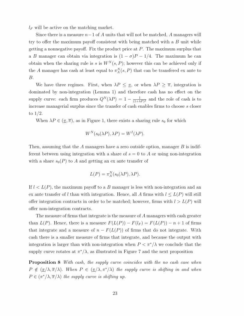
supply curve rotates at π∗/λ, as illustrated in Figure 7 and the next proposition

Proposition 8 With cash, the supply curve coincides with the no cash case when

P /∈ (π/λ, π/λ). When P ∈ (π/λ, π∗/λ) the supply curve is shifting in and when

P ∈ (π∗/λ, π/λ) the supply curve is shifting up.

23

Q

P

π/λ

π/λ

π∗/λ

Figure 7: The effect of cash

Going back to the characterization of the conflict between managers and the other

stakeholders we note two opposite effects of cash. First, there is less often inefficient

integration in the region P ∈ (π∗/λ, π/λ) and therefore output is larger and prices

lower. Second, there is more inefficient non-integration since firms stay non integrated

in the price region (π/λ, π∗/λ) while they were integrated before; since integration

is output maximizing in this region, inefficiencies increase from the point of view of

consumers and owners. This result is squarely in the second-best tradition: giving the

managers an instrument of allocation that is more efficient for them may induce them

to minimize their costs of transacting, but this may exacerbate the inefficiency of the

equilibrium contract. Here while cash reduces the over-internalization of the benefits

of coordination, it increases the over-internalization of the benefits of specialization.

This role of cash seems new to the literature.

6 Conclusion

In many models of organization, managers trade off pecuniary benefits derived from

firm revenue against private costs of implementing decisions. In our model, two key

variables affect the terms of this trade-off: product prices, over which managers have

no control, and the choice whether to integrate, over which they do. In particular,

non-integration performs well from the managerial point of view under both high and

low prices, while integration is chosen at middling prices.

24

At the same time, organizational choices also affect production: non-integration

produces relatively little output compared to integration at low prices, as managers

prefer a “quiet life”; at certain higher prices, integration can be less productive than

non-integration, despite being preferred by managers. Thus, organizational decisions

rendered by managers acting in their own interests can lead to lower output levels and

higher prices than would occur if they were forced to act in consumers’ interests. This

result is obtained even with a competitive product market, i.e., firms or managers do

not take into account the effect of reorganization or vertical integration on product

prices.

We believe that these effects can be identified in practice. For instance, the model

can identify conditions under which “waves” of integration are likely to occur – e.g.,

growing demand in an initially non-integrated industry – or when opening borders to

low cost suppliers might lead to increased product prices. More generally, as prices,

quantities, and integration decisions are easily measured, we are hopeful that models

such as the present one will encourage empirical investigations that will quantify the

real-world significance of the effects of prices on organization and vice versa.

Our analysis raises the issue of what policy remedies might be indicated to im-

prove consumer welfare. It is likely that these policies may be unconventional. For

instance, in the case of inefficient integration (where output would be higher under

non-integration), standard merger policy implemented by an antitrust authority that

blocks a potentially harmful merger may be effective in increasing output and low-

ering market prices. But the policy is surely unconventional, in the sense that it

does nothing to enhance competition, which by assumption is perfect both before

and after a proposed merger – thus it is unlikely that the antitrust authority would

be called upon to act. In the range of prices in which managers inefficiently opt not

to integrate, conventional merger policy is rather ineffective – there is no merger to

prevent.

Instead, the model suggests a novel benefit of corporate governance regulation: in

competitive markets, strengthening owners’ ability to force appropriate integration

decisions may improve consumer welfare as well as shareholder interests. In our

competitive world, shareholder and consumer interests are (nearly) aligned since they

both would value higher levels of output. However, as we have shown, even if owners

control organizational choice, their interests will typically diverge somewhat from

those of consumers.

Notice in particular that governance matters at low prices (and profitability levels)

in this model, when there is inefficiently little integration, as well as at medium-high

25

ones, where there is inefficient integration. This is in contrast to much literature

on corporate governance, which emphasizes high profit regimes as most conducive

to managerial cheating. Presumably, this is because high profit regimes are most

conducive to “profit taking,” diversion of revenues to private managerial benefits or

investments in pet projects. Our analysis underscores that governance also matters for

“profit making”: proper organizational design affects managers’ production decisions,

and is particularly important when low profitability provides weak incentives for them

to invest in a profit or output maximizing way.

Though the effects we have identified can occur absent market power, this is not

to say that market power is irrelevant to the effects of – or its effects on – major

organizational decisions. When firms have market power, incentives to integrate may

be also linked to efficiency enhancements, such as the desire to eliminate double

markups. However firms may also recognize that by reducing output they will raise

prices, and some of the effects we describe happen all the more strongly.

Moreover, the impact of “effective” corporate governance may be quite different

in this case. In a noncompetitive world, owners and consumers interests are no

longer aligned, and as we have already noted, managerial discretion may be a way

for owners to commit to low output and therefore high profits. The relative effects

of corporate governance regulation and competition policy may therefore depend non

trivially on the intensity of product market competition. These points warrant further

investigation.

26

7 Appendix

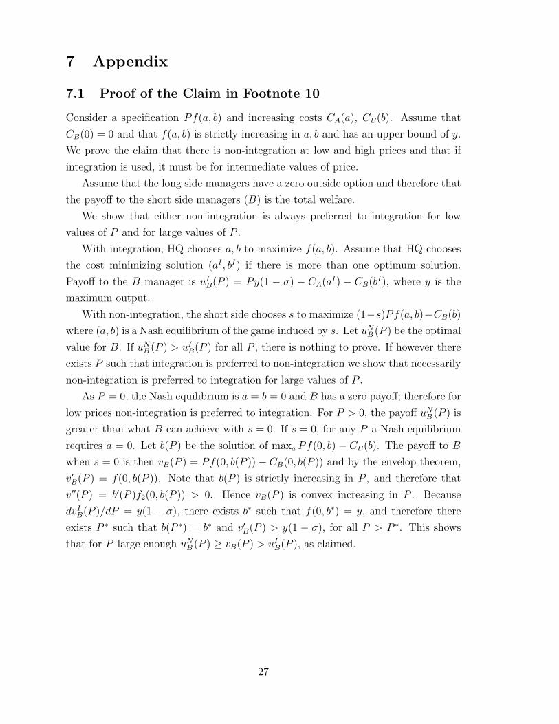
7.1 Proof of the Claim in Footnote 10

Consider a specification Pf(a, b) and increasing costs CA(a), CB(b). Assume that

CB(0) = 0 and that f(a, b) is strictly increasing in a, b and has an upper bound of y.

We prove the claim that there is non-integration at low and high prices and that if

integration is used, it must be for intermediate values of price.

Assume that the long side managers have a zero outside option and therefore that

the payoff to the short side managers (B) is the total welfare.

We show that either non-integration is always preferred to integration for low

values of P and for large values of P .

With integration, HQ chooses a, b to maximize f(a, b). Assume that HQ chooses

the cost minimizing solution (aI , bI) if there is more than one optimum solution.

Payoff to the B manager is uIB(P ) = Py(1 − σ) − CA(aI) − CB(bI), where y is the

maximum output.

With non-integration, the short side chooses s to maximize (1−s)Pf(a, b)−CB(b)

where (a, b) is a Nash equilibrium of the game induced by s. Let uNB (P ) be the optimal

value for B. If uNB (P ) > uIB(P ) for all P , there is nothing to prove. If however there

exists P such that integration is preferred to non-integration we show that necessarily

non-integration is preferred to integration for large values of P .

As P = 0, the Nash equilibrium is a = b = 0 and B has a zero payoff; therefore for

low prices non-integration is preferred to integration. For P > 0, the payoff uNB (P ) is

greater than what B can achieve with s = 0. If s = 0, for any P a Nash equilibrium

requires a = 0. Let b(P ) be the solution of maxa Pf(0, b) − CB(b). The payoff to B

when s = 0 is then vB(P ) = Pf(0, b(P ))− CB(0, b(P )) and by the envelop theorem,

v′B(P ) = f(0, b(P )). Note that b(P ) is strictly increasing in P , and therefore that

v′′(P ) = b′(P )f2(0, b(P )) > 0. Hence vB(P ) is convex increasing in P . Because

dvIB(P )/dP = y(1 − σ), there exists b∗ such that f(0, b∗) = y, and therefore there

exists P ∗ such that b(P ∗) = b∗ and v′B(P ) > y(1 − σ), for all P > P ∗. This shows

that for P large enough uNB (P ) ≥ vB(P ) > uIB(P ), as claimed.

27

7.2 Proof of Proposition 1

(i) Managerial welfare under integration is smaller than the minimum managerial

welfare under non-integration when

(1− σ)P − 1

4<

(1− 1

(1 + P )2

)P −

(P

1 + P

)2

,

⇐⇒ σ >P − 1

2P (1 + P )

⇐⇒ 2σP 2 + (2σ − 1)P + 1 > 0,

which holds whenever P is outside the interval [π, π] , where π and π are the two

solutions of the equation σ = P−12P (1+P )

.

(ii) Managerial welfare under integration is always smaller than the maximum non-

integration welfare. From (5), maximum welfare under non-integration is obtained at

s = 1/2, and welfare with integration is smaller than this maximum welfare when

(1− σ)P − 1

2<

(1− 1

(1 + P )2

)P − 1

2

(P

1 + P

)2

which simplifies to

σ > − 2 + P

2(1 + P )2− 1

2P,

which is true for all nonnegative σ since the right hand side is negative for all values

of P .

7.3 Proof of Proposition 2

Under non-integration, A gets an ex-ante payment of ω and the two managers commit

to pay D if there is success. The payoffs to the two managers given a sharing rule s

are then,

πNA (s, P,D) = s(P −D)(1− (a− b)2)− (1− a)2 + ω

πNB (s, P,D) = (1− s)(P −D)(1− (a− b)2)− b2.

Formally, from (3), the equilibrium under non-integration is Qno = 1 − 1/((1 +

P −D)2). Since the creditor makes zero profits when QD = ω, the level of debt D(ω)

when the cost is ω is obtained by solving the equation

28

ω

D= 1− 1

2(1 + P −D)2. (11)

There can be multiple solutions but the lowest repayment is also the preferred

equilibrium by the managers and is increasing in ω.

Since uA = ω, we can choose s = 0 and πNA (0, P−D(ω)) = 0 and πB = WN(0, P−D(ω)). If B is indifferent between integration and non-integration, we have

WN(0, P −D(ω)) = W I(P )− ω (12)

Observe that

WN(0, P −D(ω)) + ω = PQN(P −D(ω))− C(P −D(ω))

where C(P ) = P 2/(1+P )2. For P ′ < P, the function PQN(P ′))−C(P ′) is increasing

in P ′.18 Hence, for ω′ < ω, P −D(ω′) > P −D(ω), and

WN(0, P −D(ω′)) + ω′ > WN(0, P −D(ω)) + ω

= W I(P )

Thus B manager strictly prefers non-integration to integration when the cost is

ω′.19

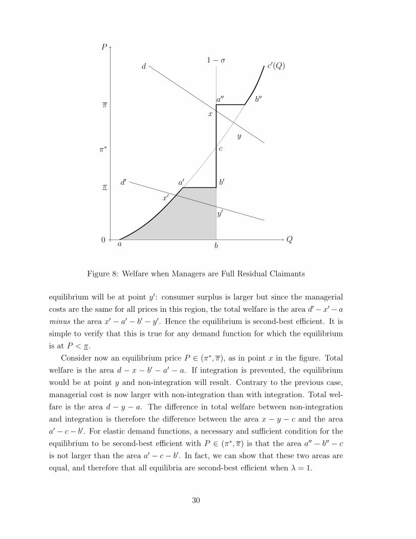
7.4 Proof that Equilibria are Second-Best Efficient if λ = 1

Suppose that managers are full residual claimant and have a revenue of P in case

of success. Clearly, if an organization maximizes managerial welfare and is output

maximizing, it is also second-best efficient. Hence, at prices P > π and prices P ∈(P , P ∗] equilibria are second-best efficient. For the other cases, it is convenient to

consider first the case of zero outside option of A; we will refer below to Figure 8.

The managerial cost under integration is the shaded area.

Consider first the case P < π and a typical demand function d′. Industry equi-

librium is at x′ and total welfare is the area d′ − x′ − a. If integration is “forced”,

18Derivation with respect to P ′ yields the expression (P −P ′)((1+P ′)3) which is positive becauseP ′ < P .

19The same reasoning holds for any initial share s ∈ (0, 1/2). Because uA(s, ω′, P ) = πNA (s, P −D(ω′)) + ω′ and πNA is increasing in P −D(ω), we have uA(s, ω′, P ) > ω′. The optimal value of sunder ω′ will therefore be s′ < s, which will further increase the payoff to B under non-integrationwhile the payoff under integration is the same.

29

0 Q

P

b

1− σ

a

c′(Q)

π∗

π

π

a′ b′

d

x

c

y

a′′ b′′

d′

x′

y′

Figure 8: Welfare when Managers are Full Residual Claimants

equilibrium will be at point y′: consumer surplus is larger but since the managerial

costs are the same for all prices in this region, the total welfare is the area d′− x′− aminus the area x′ − a′ − b′ − y′. Hence the equilibrium is second-best efficient. It is

simple to verify that this is true for any demand function for which the equilibrium

is at P < π.

Consider now an equilibrium price P ∈ (π∗, π), as in point x in the figure. Total

welfare is the area d − x − b′ − a′ − a. If integration is prevented, the equilibrium

would be at point y and non-integration will result. Contrary to the previous case,

managerial cost is now larger with non-integration than with integration. Total wel-

fare is the area d − y − a. The difference in total welfare between non-integration

and integration is therefore the difference between the area x − y − c and the area

a′ − c− b′. For elastic demand functions, a necessary and sufficient condition for the

equilibrium to be second-best efficient with P ∈ (π∗, π) is that the area a′′ − b′′ − cis not larger than the area a′ − c− b′. In fact, we can show that these two areas are

equal, and therefore that all equilibria are second-best efficient when λ = 1.

30

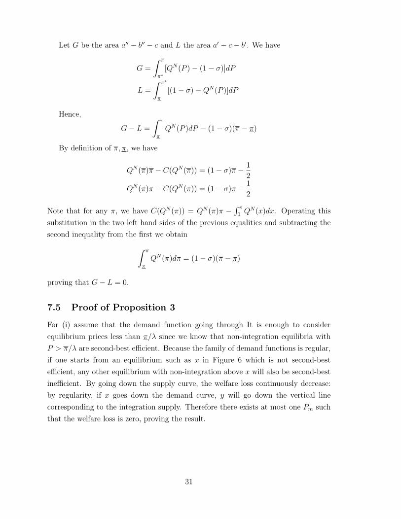
Let G be the area a′′ − b′′ − c and L the area a′ − c− b′. We have

G =

∫ π

π∗[QN(P )− (1− σ)]dP

L =

∫ π∗

π

[(1− σ)−QN(P )]dP

Hence,

G− L =

∫ π

π

QN(P )dP − (1− σ)(π − π)

By definition of π, π, we have

QN(π)π − C(QN(π)) = (1− σ)π − 1

2

QN(π)π − C(QN(π)) = (1− σ)π − 1

2

Note that for any π, we have C(QN(π)) = QN(π)π −∫ π

0QN(x)dx. Operating this

substitution in the two left hand sides of the previous equalities and subtracting the

second inequality from the first we obtain∫ π

π

QN(π)dπ = (1− σ)(π − π)

proving that G− L = 0.

7.5 Proof of Proposition 3

For (i) assume that the demand function going through It is enough to consider

equilibrium prices less than π/λ since we know that non-integration equilibria with

P > π/λ are second-best efficient. Because the family of demand functions is regular,

if one starts from an equilibrium such as x in Figure 6 which is not second-best

efficient, any other equilibrium with non-integration above x will also be second-best

inefficient. By going down the supply curve, the welfare loss continuously decrease:

by regularity, if x goes down the demand curve, y will go down the vertical line

corresponding to the integration supply. Therefore there exists at most one Pm such

that the welfare loss is zero, proving the result.

31

7.6 Proof of Proposition 5

(1) Note that vN(0) = 0 > vI(0). On the other hand, vN(P ∗) < vI(P ∗): by definition,

vN(P ∗) =(

1− 1(1+π∗)2

)(P ∗ − π∗) = (1 − σ)(P ∗ − π∗) < (1 − σ)(P ∗ − π), since

π < π∗. Moreover, the marginal payoffs satisfy vN ′(P ∗) = vI′(P ∗) = 1 − σ; thus for

P > P ∗, vN ′(P ) > vI′(P ), and for P < P ∗, v′N(P ) < v′I(P ) and we conclude that

vN(·) = vI(·) at two prices P0 and P ′1, with 0 < P0 < P ∗ < P ′1. Since QN(π) < 1− σ,vN(P ) < vI(P ). Therefore, P0 < P.

As for P ′1 however, we do not know if it is greater than P . If it is, then π∗(P ′1) > π

and managers will indeed choose non-integration if they are offered the compensation

π∗(P ′1); using P1 = P ′1 proves the result.

If however π∗(P ′1) < π, managers will choose integration while owners want to

implement non-integration.20 If the owners are implementing non-integration, they

must offer a compensation π /∈ (π, π) for prices in the interval [P , P ]. Remember

that the slope of vN(P ) is QN(π). It follows that using a compensation π cannot be

optimal since integration dominates (the graph of the payoff function QN(π)(P − π)

is tangent to the graph of vN(P ) at P = P and is therefore strictly lower than vI(P )

for prices greater than P .) For a compensation of π however, the payoff with non-

integration is equal to the integration payoff for a price P1 in the interval (P ′1, P ),

proving the result.

(2) If σ > σ, managers always prefer non-integration and the result follows.

7.7 Outside Options

Let F (uA) and G(uB) be the distributions of outside options for A and B respectively,

with supports [0,∞). We assume that F andG have continuous and positive densities.

Let u be a payoff to A and φno(u;P ) and φint(u;P ) be the frontiers of the non-

integration and integration cases when the price is P . The overall frontier is φ(u;P ) =

max{φno(u;P ), φint(u;P )}.

Lemma 9 Fix a price P . There exists a unique value α(P ) such that F (α) = G(β)

and β = φ(α;P ). Moreover, this solution is increasing in P .

Proof. The function h(α) = G−1(F (α)) is well defined since the densities are positive.

Moreover, as α increases, h(α) strictly increases. Now φ(α;P ) is strictly decreasing

in α. It follows that there exists a unique value solving h(α) = φ(α;P ); this solution

20The necessary and sufficient condition for having P ′1 < P is P > QN (π)π−(1−σ)πQN (π)−(1−σ)

.

32

is increasing in P because φ(α;P ) is increasing in P .

We will write that a firm improves on outside options whenever uB ≤ φ(uA;P ).

Proposition 10 In a supplier market equilibrium, firms that can improve on outside

options consist of A-managers with outside options uA ≤ α(P ) and B-managers with

outside options uB ≤ h(α(P )). All A managers have payoff α(P ) and all B-managers

have payoff h(α(P )).

Proof. Consider an equilibrium in the supplier market with sets IA and IB of man-

agers, where we identify (wlog) a manager with an outside option. Consider a firm

(uA, uB) that improves on outside options and let (πA, πB) be the equilibrium payoffs.

Suppose that manager u′A < uA is not in a firm. Then this manager gets her outside

option. Because the frontiers are strictly decreasing and firms improve on outside

options, πB = φ(πA;P ) ≤ φ(uA;P ) < φ(u′A;P ). Hence, there exist π′B > πB and

π′A > u′A satisfying π′B = φ(π′A;P ), contradicting stability. A similar argument shows

that all managers with outside options u′B < uB must be in equilibrium firms.

Let [0, α) be the set A-managers in firms. By measure consistency, the set of

B-managers is [0, h(α)]. We claim that all A-managers get the same payoff and all

the B-managers get the same payoff. If, for instance, there are two A-managers have

different payoffs πi < πj, consider the B-manager k who is in a firm with j. Since

firms improve on outside options, k gets her outside option by matching with j: hence

k will obtain a strictly higher payoff by matching with the A-manager i and offering

a payoff in the interval (πi, πj). Hence all A-managers get the same payoff πA. A

similar argument shows that all B-managers get the same payoff πB. Because firms

improve on outside options, it must be the case that πA ≥ α and that πB ≥ h(α).

If α < α(P ), then πA + πB > α + h(α). Without loss of generality, assume that

πB > h(α), then there exists ε > 0 such that πB > h(α) + ε. But then there exists

δ > 0 such that a B-manager with outside option h(α) + ε can offer a A-manager

πA + δ while getting for herself strictly more than her outside option, contradicting

the assumption that this manager is not in a firm. Hence α = α(P ) as claimed,

proving the proposition.

This proposition is useful because it suggests that the way the surplus is shared

in equilibrium depends on the slope of the curve h(α). In particular we have the

following.

Corollary 11 Suppose that F = G, then for any price P and any σ non-integration

is chosen.

33

Indeed, if the two sides have the same distributions of outside options, h(α) = α and

in equilibrium, the payoffs are πA = πB = α(P ). Because non-integration dominates

integration when A and B get the same payoff, non-integration will be the equilibrium

organization for any value of P , even if σ = 0.

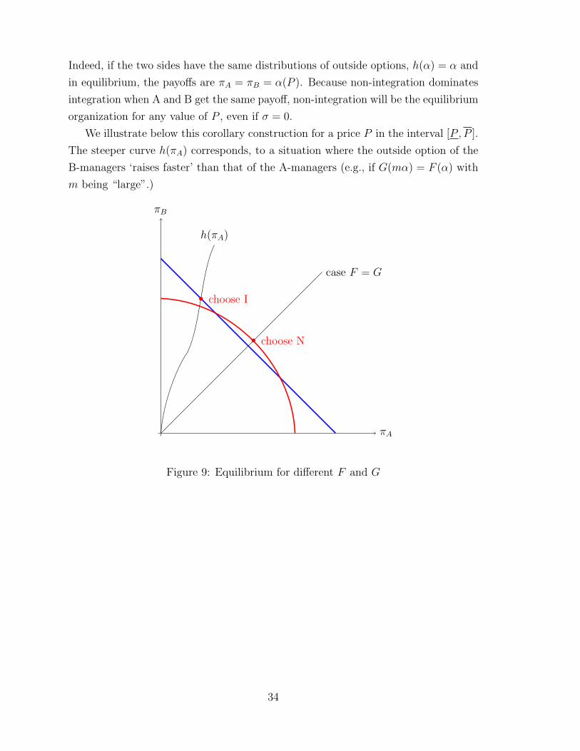
We illustrate below this corollary construction for a price P in the interval [P , P ].

The steeper curve h(πA) corresponds, to a situation where the outside option of the

B-managers ‘raises faster’ than that of the A-managers (e.g., if G(mα) = F (α) with

m being “large”.)

πA

πB

h(πA)

choose I

case F = G

choose N

Figure 9: Equilibrium for different F and G

34

References

[1] Acemoglu, D., S. Johnson and T. Mitton (2007) “Determinants of Verti-

cal Integration: Financial Development and Contracting Costs,” http://econ-

www.mit.edu/files/221

[2] Alchian, Armen A and Harold Demsetz (1972), “Production, Information Costs,

and Economic Organization,” American Economic Review, 62: 777-795.

[3] Bolton, Patrick, and Mathias Dewatripont (1994), “ The Firm as a Communi-

cation Network,” Quarterly Journal of Economics 109: 809-839.

[4] Bertrand, Marianne and Sendhil Mullainathan (2003), “ Enjoying the Quiet

Life? Corporate Governance and Managerial Preferences,” Journal of Political

Economy, 111(5): 1043-1075.

[5] Ethier, Wilfred J.(1986), “The Multinational Firm,” Quarterly Journal of Eco-

nomics 101: 805-833.

[6] Fama, Eugene F., and Michael C. Jensen (1983), “ Separation of Ownership and

Control,” Journal of Law and Economics, 26: 301-325.

[7] Ghemawat, Pankaj (2001), “ Global vs. Local Products: A Case Study and A

Model,” mimeo, Harvard Business School.

[8] Grossman, Sanford and Oliver Hart (1986), “ The Costs and Benefits of Owner-

ship: A Theory of Vertical and Lateral integration,” Journal of Political Econ-

omy, 94:4 691-719.

[9] Grossman, Gene and Elhanan Helpman (2002), “ Outsourcing Versus FDI in

Industry Equilibrium,” CEPR DP 3647.

[10] Hart, Oliver (1983), “The Market Mechanism as an Incentive Scheme” Bell Jour-

nal of Economics 14(2): 366-382.

[11] Hart, Oliver, and Bengt Holmstrom (2002), “ A Theory of Firm Scope,” mimeo

Harvard University.

[12] Hart, Oliver and John Moore (1999), “ On the Design of Hierarchies: Coordi-

nation versus Specialization,” National Bureau of Economic Research Working

Paper: 7388.

35

[13] Jensen, Michael C. (1986), “Agency Cost of Free Cash Flow, Corporate Finance,

and Takeovers,” American Economic Review, 76(2):323-329.

[14] Jensen, Michael C. and William H. Meckling (1976), “Theory of the Firm: Man-

agerial Behavior, Agency Costs, and Ownership,” Journal of Financial Eco-

nomics, 3:305-60.

[15] Khanna, Tarun, and Krishna Palepu (1997), “Why Focused Strategies May Be

Wrong for Emerging Markets,” Harvard Business Review 75:4, 41-51.

[16] (2000), “Is Group Affiliation Profitable in Emerging Markets? An Anal-

ysis of Diversified Indian Business Groups,”Journal of Finance 55: 867-891.

[17] Legros, Patrick and Andrew F. Newman (1996), “Wealth Effects, Distribution,

and the Theory of Organization” Journal of Economic Theory, 70(2): 312-41.

[18] (2006), “Managerial Firms, Organizational Choices and Consumer Sur-

plus” mimeo.

[19] (forthcoming), “ Competing for Ownership,” Journal of the European

Economic Association.

[20] Leibenstein, Harvey (1966), “ Allocative Efficiency vs. ‘X-Efficiency’,” American

Economic Review 56(3): 392-415.

[21] Levy, B. (1990) “Transactions Costs, the Size of Firms and Industrial Policy:

Lessons from a Comparative Case Study of the Footwear Industry in Korea and

Taiwan” Journal of Development Economics, 34 (1-2): 151-178.

[22] Mailath, George, Volker Nocke and Andrew Postlewaite (2002), “ The Disincen-

tive Effects of Internalizing Externalities,” mimeo University of Pennsylvania.

[23] Mitchell, Mark L., and J. Harold Mulherin (1996), “ The Impact of Industry

Shocks on Takeover and Restructuring Activity,” Journal of Financial Eco-

nomics, 41: 193-229.

[24] Powell, Ronan G., and Alfred Yawson (forthcoming), “ Industry Aspects of

Takeovers and Divestitures: Evidence from the U.K.,” Journal of Banking and

Finance.

[25] Radner, Roy (1993), “ The Organization of Decentralized information Process-

ing,” Econometrica, 62, 1109-1146.

36

[26] van den Steen, Eric (2005), “ Organizational beliefs and managerial vision,”

Journal of Law, Economics, and Organization, 21, pp. 256283.

[27] White, Lawrence (2002), “ Trends in Aggregate Concentration in the United

States,” Journal of Economic Perspectives, 16(4): 137-160.

[28] Williamson, Oliver E. (1986), “ Hierarchical Control and Optimum Firm Size,”

in Oliver Williamson Economic Organization: Firms, markets and policy control,

New York: New York University Press 1986; 32-53. Previously published: 1967.

[29] Woodruff, C. (2002) “Non-contractible Investments and Vertical Integration in

the Mexican Footwear Industry”, International Journal of Industrial Organiza-

tion, 20: 1197-1224.

37