Embed Size (px)
Citation preview
Competition and Academic Performance: Evidencefrom a Classroom Experiment ∗
Kelly BedardUniversity of California, Santa Barbara and IZA
Stefanie FischerCal Poly State University, San Luis Obispo
July 21, 2017
Abstract
We examine the effect of relative evaluation on academic performance by implementing aclassroom-level field experiment in which students are incentivized individually or in a tour-nament to take a microeconomics quiz. We focus on two aspects of competitive environmentsthat may be particularly salient in academics: tournament size and one’s perceived position inthe ability distribution. At least in our setting, we find no evidence that effort responses to com-petition are sensitive to tournament size. However, in contrast to previous studies that examineeffort responses to exogenously assigned competition, we find a large negative competitioneffect for students who believe they are relatively low in the ability distribution and no compe-tition effect for those who believe they are relatively high ability. Using additional treatments,we further show that the divergence between our results and past results is driven by task typeand not by differences in selection into participation between lab and field environments.
∗We thank the office of Institutional Research, Planning and Assessment at UC Santa Barbara for access to adminis-trative data. We also thank the UCSB economics and accounting instructors who donated class time to the experiment.This paper has benefited from helpful comments from Jenna Stearns, Gary Charness, Aric Shafran, Brian Duncan,Rey Hernandez-Julian, and seminar participants at the Federal Reserve Bank of New York and Claremont McKennaCollege. All errors are our own.
2
1 Introduction
Success in higher education often hinges on relative performance. Admission to selective colleges
is in large part determined by class rank and relative scores on entrance exams. Undergraduate
grades are often assigned using a curve. And, graduate and professional schools rely heavily on
standardized tests to determine admission. This paper adds to the growing literature examining ef-
fort responses to competition by exploring student responses to competition in a classroom setting.
More specifically, we administer a controlled experiment in university economics classes where
students are incentivized to take a short introductory microeconomics quiz. We focus on two as-
pects of competitive environments that may be particularly salient in academics: one’s perceived
position in the ability distribution and tournament size.
Economic theory offers important insights into possible effort responses to competitive condi-
tions. For example, Brown (2011) shows that ability gaps (or perceived gaps) between competitors
can result in reduced effort for weaker contestants. She provides empirical support for her model
using data from professional golf. More specifically, she shows that competitors perform worse
when Tiger Woods plays in a tournament, at least back in his prime. In a different vein, Andreoni
and Brownback (2014) model effort responses to competition when group size varies (holding the
proportion of winners constant).1 As class size shrinks, students become less certain about their
rank. They show that this uncertainly leads low ability students to increase effort because working
hard increases their chance of earning a high grade, but decreases the effort level of high ability
students because there is still little risk of losing out on a top grade. Stated somewhat differently, as
a class grows in size, it approaches the population and students know their exact percentile rank. In
an infinitely large class, high types who are at or above the winning threshold will exert a positive
amount of effort, those below the winning threshold will exert no effort. However, when Andreoni
and Brownback (2014) take this to the lab, they find no real difference between individual’s bids
and the size of group at either end of the valuation distribution (or what translates into the ability
1Their model builds on work by Lazear and Rosen (1981), Becker and Rosen (1992) and Orrison et al. (2004).
3
distribution) in an all-pay auction.2
While models help build intuition, generally speaking, in environments outside the lab where
there is less control over the parameters of the experiment, predicting effort responses is difficult.
In other words, student effort responses to competition, and whether or not they vary systemat-
ically by ability and group size are in the end empirical questions. Our objective is to examine
how effort changes in response to competition in a classroom setting, and to further ask whether
responses differ across ability groups and/or the size of the tournament with which one is forced to
compete. To do this, we run randomized experiments at the beginning of economics classes early
in the academic quarter. Students are randomly assigned across a variety of tournament structures
in which their earnings depend on their own quiz performance relative to their opponent’s perfor-
mance. To isolate the causal effect of competition, we also include a non-competitive piece rate
treatment in which subjects are paid a flat rate for each correct answer. We find a large negative
competition effect for students who believe they are a relatively low scoring student. In particular,
students who believe they will earn less than an “A” grade in their current economics course score
about 22 percent of a standard deviation lower when forced to compete compared to students as-
signed to the piece rate treatment.3 We will refer to these students as low expectation students. In
contrast, there is no statistically significant difference in quiz scores between tournament and piece
rate subjects for those who believe they will earn an “A”. We will refer to these students as high
expectation students. Consistent with previous lab studies, e.g., Lima et al. (2014) and Andreoni
and Brownback (2014), we find no evidence that these results vary across tournament size.
We are, of course, not the first to study effort responses to forced competition. In all cases,
effort is either modeled as a cost chosen off a menu in a laboratory setting (Bull et al., 1987;
Orrison et al., 2004) or as actual effort on a simple task such as solving mazes, running, adding
2Others have studied the effects of varying group size while maintaining the number of winners; e.g., Barut et al.(2002) and Lima et al. (2014). Lima et al. (2014) consider the effect of group size in a lab in an across-subjects designwhere subjects play a Tullock contest game. They find the average expenditure does not differ significantly acrossgroups of two, four, or nine when there is a single winner.
3For context, approximately 60 percent of students believe that they will earn an A or an A- (what we refer to asan “A” grade), despite the fact that the actual number of such grades awarded is far below this level. We explore thedifference between expected grades and actual earned grades in Section 5.1.
4
up numbers, or solving word and memory puzzles (Gneezy et al., 2003; Gneezy and Rustichini,
2004; Günther et al., 2010; Dreber et al., 2014). In contrast to our results, these studies generally
find that individuals who are forced to compete, work at least as hard as those who are not; though
there is some evidence suggesting the competition effect is sensitive to task type.4
There are two obvious candidate explanations for the divergence between our results and those
reported in previous studies: task type and selection into participation. We explore these possibil-
ities by running two additional treatments. In the first we replace the microeconomics quiz with a
simple numeric task that is more similar to previous experiments. Interestingly, in these rounds we
find no difference across competitive and piece rate payment schemes for either low or high ex-
pectation students – the weaker students exert less effort under competition result vanishes. In the
second additional treatment we move the experiment (using the same microeconomics quiz) to the
end of section and tell students that they are free to stay and participate or to leave. Approximately
fifty percent of students choose to leave. The results for these rounds are similar to the rounds
that are run at the beginning of section. In other words, we find no evidence that our competition
results are driven by selection into participation.
The findings in this study offer at least two new insights. First, in our classroom context where
students are asked to complete a real-effort and ability-specific task, we show that responses to
competition depend on perceived ability. When forced to compete, low expectation students work
less hard and high expectation students do not change their effort level. If it is the goal of the
instructor or policymaker is to improve effort and thus academic outcomes, our results suggest
that competition may not be the optimal mechanism, at least for those who perceive themselves as
relatively low ability. Second, the fact that results from rounds of the experiment where a more
general skill task is used – one similar to those used in previous studies – differ from the results
for the microeconomics quiz, arguably a more specialized skill task, suggests that one should be
4There is a closely related experimental literature examining the propensity of individuals to compete when offeredthe choice. This literature finds that women are less likely to choose competition over a piece rate option compared tomen (Niederle and Vesterlund, 2007; Gneezy et al., 2009; Sutter and Rutzler, 2015; Booth and Nolen, 2012a; Villeval,2012; Datta Gupta et al., 2013; Garratt et al., 2013). There also exists an extensive theoretical literature focused onunderstanding effort response to relative performance incentive schemes, examples include Lazear and Rosen (1981),Green and Stokey (1983), and Prendergast (1999). See List et al. (2014) for a review.
5
cautious generalizing about effort responses to competition across task type.
2 Experimental Design
2.1 Microeconomics Quiz with No Selection into Participation
We administered the primary treatments to 2,415 students in 70 economics sections/classes at the
University of California, Santa Barbara (UCSB) from fall 2013 through summer 2015. All sessions
were held during the first two weeks of the relevant quarter. Before students entered the classroom
sealed envelopes containing an entry survey and a microeconomics quiz were distributed across
seats such that treatment groups were seated together. As students entered the section, they were
randomly assigned to a treatment group by receiving a ticket from a shuffled deck that assigned
them to a particular seat. Students who arrived late were asked to wait outside until the experiment
ended. In all cases this was a very small number of students as we waited several minutes after the
usual start time to close the door.
Once entry into the room had ceased, students completed an entry survey. This was a short
questionnaire asking about their age, race, gender, year in school, intended major, and the grade
they expect to earn in the course in which the quiz was being administered (the survey is in Ap-
pendix A). Importantly, we classify students into two groups based on how they respond to the
entry survey question, “What grade do you expect to earn in this class?”. We define those who
believe they are going to earn an “A” as high expectation students, and those who indicate they
expect to earn a grade less than an “A” as low expectation students. This allows us to separately
analyze effort responses to competition across perceived ability and and tournament size. For con-
text, approximately 66 percent of students expect to earn an “A” in the current course. We will
explore differences between perceived ability and actual ability in Section 5.1.
Next we explained that we were administering a microeconomics quiz in a large number of
sections across both lower and upper division economics courses. We also informed participants
that we would be coming around to explain how they could earn money for correctly answering
6
quiz questions and that they would be entered into a $25 drawing at the end of the quiz to thank
them for participating. At least in part because the quiz was administered at the beginning of
classes and sections, participation was essentially 100 percent; less than five students left during
the instruction phase and did not fill out a survey or participate in the quiz.
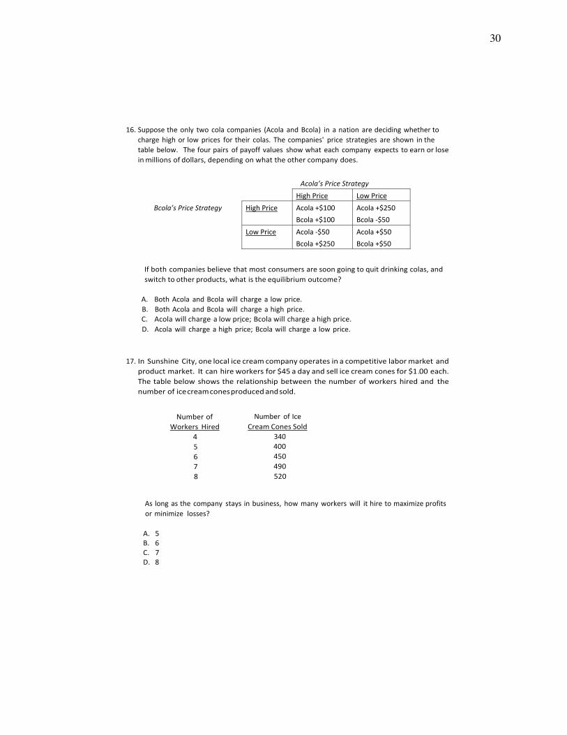
Students were given fifteen minutes to complete a ten question microeconomics quiz. They
were not permitted to use a calculator or any other materials. We used six quiz forms to guard
against cheating. The questions on each form were randomly drawn within subject category from
the Test of Understanding in College Economics (TUCE) exam. The TUCE is a 30 question
introductory microeconomics exam given to college economics students across the United States.
An example of the quiz is in Appendix A. Students were incentivized for each correct quiz answer
based on their randomly assigned treatment group. The treatment groups were as follows:
1. Piece Rate: Subjects earned $0.50 for each correct answer.
2. Group of Two: The subject with the highest score in each pair earned $1 for each correct
answer.
3. Group of Six, Top Half Paid: The three highest scoring subjects in each group earned $1 for
each correct answer.
4. Group of Ten, Top Half Paid: The five highest scoring subjects in each group earned $1 for
each correct answer.
5. Group of Six, Winner Take All: The subject with the highest score in each group earned $3
for each correct answer.
6. Group of Ten, Winner Take All: The subject with the highest score in each group earned $5
for each correct answer.
The baseline treatment incentivizes students using a non-competitive piece rate payment scheme.
Treatments two through four maintain the proportion of winners but vary group size. One can think
7
of this type of design as grading on a curve, where the same share of the class (e.g., 20%) always
earns an “A” grade. In contrast, treatment groups five and six vary group size but have a single
winner. Note that the ex ante expected value would be the same across all treatments if quiz scores
were randomly assigned. Using a wide range of tournament sizes and payout structures is intended
to allow for the detection of any or all possible group size effects.
Ties were broken by random draw. Given the number of groups, not all treatments were ad-
ministered in every section, but more than one group was administered in every section. This is
important because it allows for the inclusion of section fixed effects.
2.2 Task Type
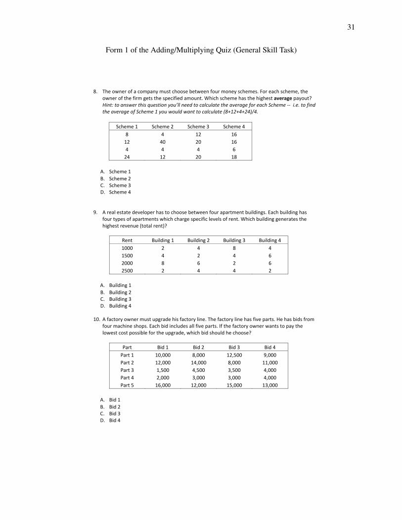
As it is possible that responses to competition depend on the type of task, in summer 2015 we also
compared performance on the microeconomics quiz – a specialized skill task – to a relatively more
general skill based quiz. This general skill quiz more closely resembles the tasks used in much of
the previous experimental literature on competition; it required students to add and multiple two
digit numbers without a calculator. To examine whether the effects of competition depend on task
type, we randomly assigned 180 students in 11 sections into one of four treatment groups: piece
rate and a TUCE quiz, piece rate and an adding/multiplying quiz, group of two and a TUCE quiz,
or group of two and an adding/multiplying quiz. For tractability, we limit group size to two in this
round. The incentive structure is the same as above: $0.50 per correct answer in piece rate and $1
for each correct answer for the highest scoring student in the group of two tournament. Because
the adding/multiplying and TUCE quizzes were administered simultaneously in all 11 sections, the
former was formatted to look like a microeconomics quiz; calculating rent, minimum cost, average
return, and so on. An example of the adding/multiplying quiz is included in Appendix A.
2.3 The Role of Selection into Participation
In contrast to most lab experiments, our environment features very different selection. In our
setting, conditional on attending the chosen section, we have essentially 100 percent participation.

8
This occurs by design because all experiments were run at the beginning of section. On the other
hand, in a typical lab setting, students are recruited through a web based application and must show
up to the lab at a designated time solely for the purpose of participating in the experiment.
In an effort to understand how our sample compares to a group that is relatively more selected,
we ran 11 sessions in summer 2015 during the last 15 minutes of sections. On these occasions,
students could choose to stay and participate in the quiz or to leave. They were told that they
could earn money for correctly answering quiz questions and that they would be eligible to win
a $25 raffle for their participation. Roughly half of students in these sections chose to stay and
participate in the experiment. Those who stayed were randomly assigned to a piece rate or group
of two treatment. As in all other sessions, those in the piece rate group earned $0.50 for each
correct answer and the top scorer in the group of two earned $1.00 for each correct answer. 137
students participated in these rounds.
3 Subjects and Data
All data come from two sources. The main source is the data collected directly from the survey
and experiment. The experiments were conducted in four rounds: fall quarter 2013, spring quarter
2015, and summer sessions A and B 2015. We ran experiments in 81 sections with 2,732 total
participants at UCSB. These data include quiz scores, treatment assignments, race, gender, major,
academic year standing, age, and the grade they expect to earn in the course in which the quiz is
administered. All tables are restricted to participants who responded to all questions on the survey
and for whom we can standardize their test score.5 These restrictions eliminate 143 participants,
leaving an estimating sample of 2,589. Table 1 reports summary statistics for quiz scores, stan-
dardized quiz scores, and expected grade disaggregated by the six main treatments (Panel A), by
gender (Panel B), and class standing (Panel C). The sample in Table 1 is restricted to the 2,298 par-
ticipants who took the TUCE quiz at the beginning of a section. We provide similar information
5All scores are standardized by quiz form within each course in a given quarter. By bad luck, 21 students receiveda test form that no one else in their class received, making it impossible to calculate a standardized score.
9
for those who took the more general skill task and the rounds that were run at the end of sections
in Section 6. While column 1 reports raw TUCE quiz scores to give the reader some context, col-
umn 2, and all columns in all subsequent tables use scores that are standardized to mean zero and
standard deviation one by course, year, and quiz form.
It is worth highlighting a few features of Table 1. The average TUCE quiz score is approxi-
mately 5 out of 10, the average male undergraduate outscores the average female undergraduate,
and students in upper division courses outscore students in lower division courses. While the av-
erage score is also highest for the piece rate group, it is important to remember that there are no
controls and not all treatments were assigned in every section. Roughly two-thirds of the partic-
ipants have high expectations (expect to earn an “A” grade) in the current course and on average
women are somewhat less likely to have high expectations.
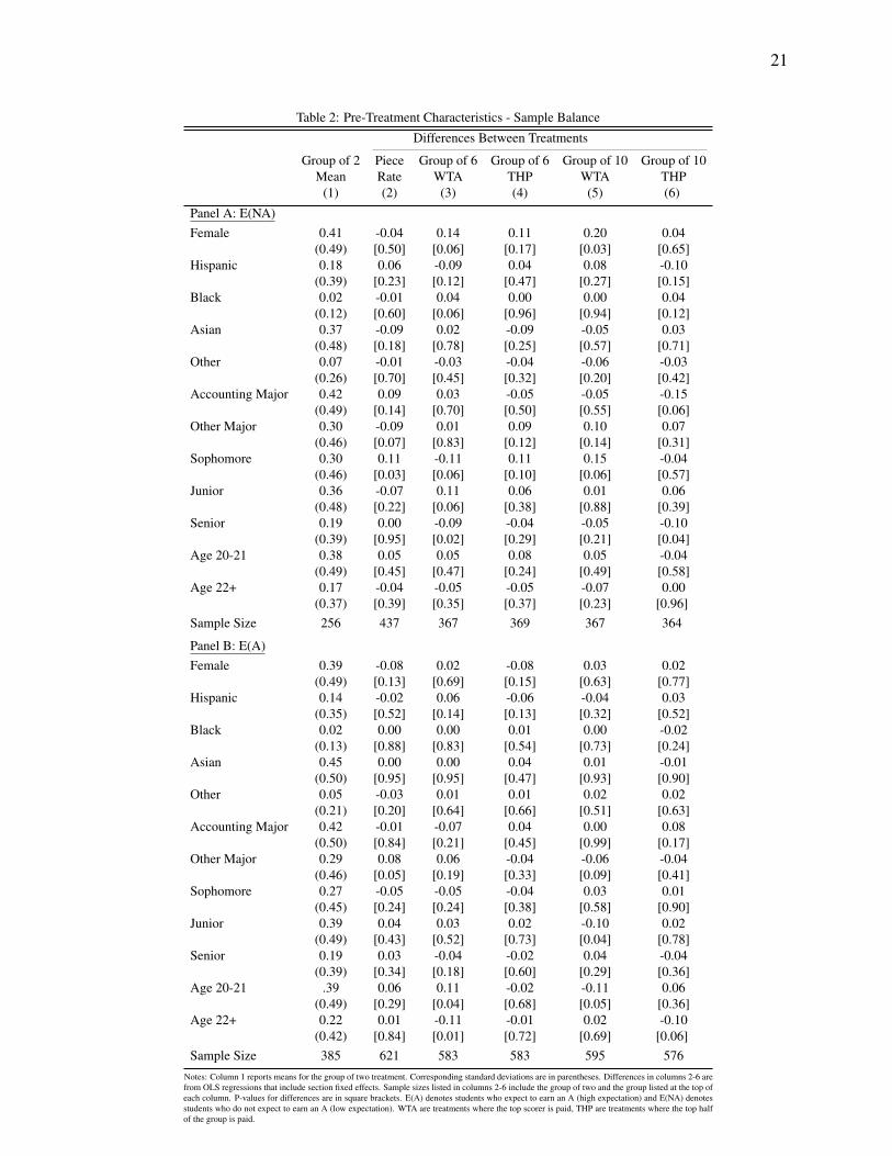
Panel A of Table 2 reports descriptive statistics for the pre-treatment characteristics collected
on the entry survey for low expectation participants. Column 1 reports the mean and standard
deviation for each characteristic for participants assigned to the group of two treatment. Columns
2-6 report the differences in mean characteristics between the group of two and each of the other
treatment groups. Each entry in these columns comes from a separate regression. There is little
evidence of systematic differences in gender, race, major, class standing, or age across treatment
groups. Panel B replicates this exercise for high expectation participants. Again, there is little
evidence of imbalance across treatment groups, at least based on observable characteristics.
The experiment and survey data are also linked to administrative records that include infor-
mation about parental education, transfer status, language spoken in the home, citizenship status,
socioeconomic status, SAT scores, and grades earned in core economics courses at UCSB. Unfor-
tunately, there are many non-random missing values for all variables in the administrative data. For
instance, administrative records do not contain SAT scores for transfer students. As such, our pre-
ferred specifications use the measures drawn from the survey, but not the variables collected from
administrative records. The primary deviation from this will be a heterogeneity analysis that ex-
plores the relationship between expected grades and actual grades. These issues will be discussed
10
in more detail in Section 5.1.
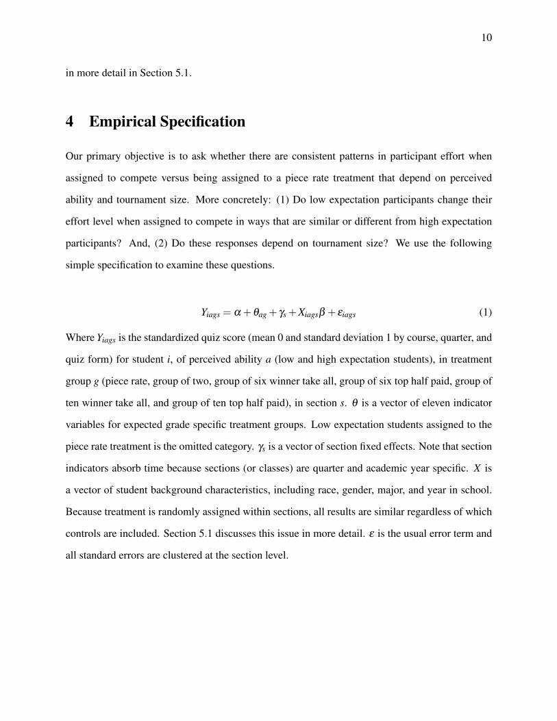
4 Empirical Specification
Our primary objective is to ask whether there are consistent patterns in participant effort when
assigned to compete versus being assigned to a piece rate treatment that depend on perceived
ability and tournament size. More concretely: (1) Do low expectation participants change their
effort level when assigned to compete in ways that are similar or different from high expectation
participants? And, (2) Do these responses depend on tournament size? We use the following
simple specification to examine these questions.
Yiags = α +θag + γs +Xiagsβ + εiags (1)
Where Yiags is the standardized quiz score (mean 0 and standard deviation 1 by course, quarter, and
quiz form) for student i, of perceived ability a (low and high expectation students), in treatment
group g (piece rate, group of two, group of six winner take all, group of six top half paid, group of
ten winner take all, and group of ten top half paid), in section s. θ is a vector of eleven indicator
variables for expected grade specific treatment groups. Low expectation students assigned to the
piece rate treatment is the omitted category. γs is a vector of section fixed effects. Note that section
indicators absorb time because sections (or classes) are quarter and academic year specific. X is
a vector of student background characteristics, including race, gender, major, and year in school.
Because treatment is randomly assigned within sections, all results are similar regardless of which
controls are included. Section 5.1 discusses this issue in more detail. ε is the usual error term and
all standard errors are clustered at the section level.
11
5 Results
5.1 Economics Quiz at the Beginning of Section
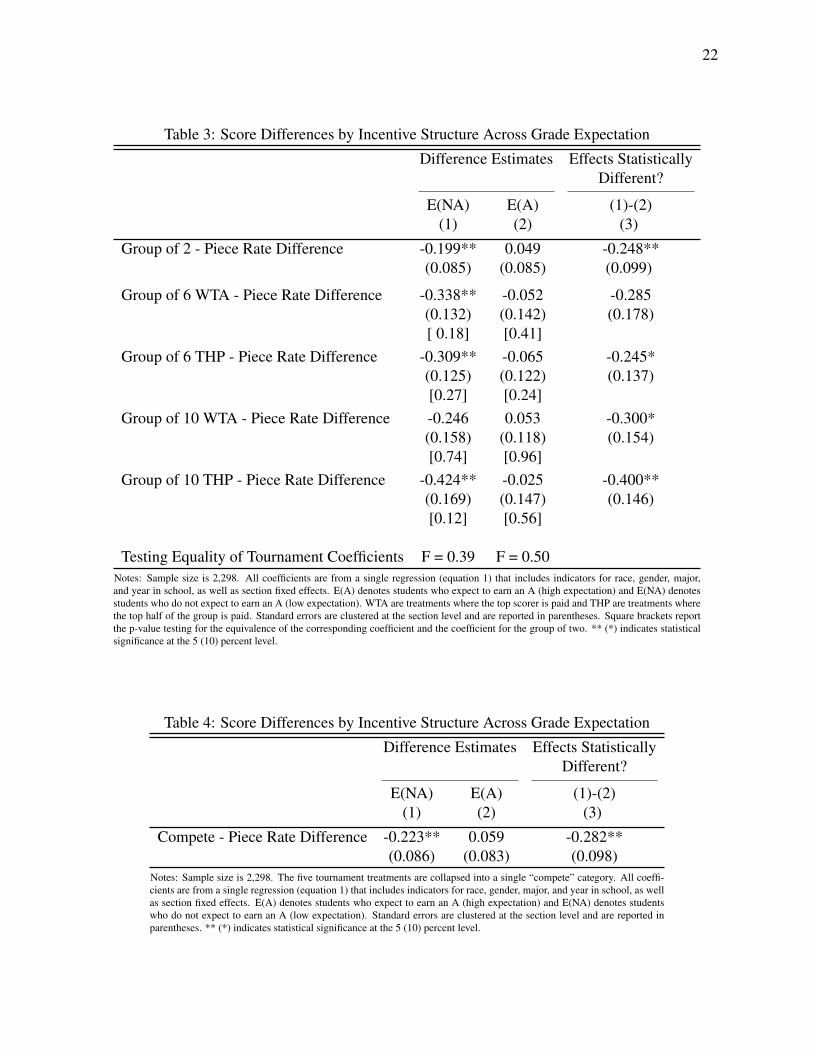
The results for equation 1 are reported in Table 3. Unless otherwise specified, all point estimates in
each table come from a single regression. Column 1 reports the difference in quiz score between
the piece rate treatment and each of the five tournament treatment groups for low expectation par-
ticipants. P-values for the difference in competition effect between the specified larger tournament
size and the group of two for low expectation students are reported in square brackets under the
standard errors. Column 2 reports the same set of results for high expectation students. In other
words, each entry tells you the average difference in scores between the specified group and the
piece rate group for individuals who expect a high grade. Similarly, the p-values reported in square
brackets are for the difference in competition effect between the group of two and the specified
larger group for high expectation students. Column 3 reports the difference between the low and
high expectation student groups within each tournament size.
Column 1 reveals that low expectation students reduce their effort when forced to compete.
More specifically, the average group of two score is 19.9 percent of a standard deviation lower than
the average piece rate score; for context, 25 percent of a standard deviation is approximately half
a point on the ten-point TUCE quiz. Further, there is no evidence that the size of the tournament
or the pay structure matters; we fail to reject the null hypothesis that the point estimate for any
tournament group larger than two is the same as for the group of two.6 In contrast, there are
no precisely estimated competition effects for high expectation students at any tournament size.
Column 3 shows that the competition effects for the two ability groups are statistically different
from one another, and that is the case for all but one of the tournament group sizes. Appendix Table
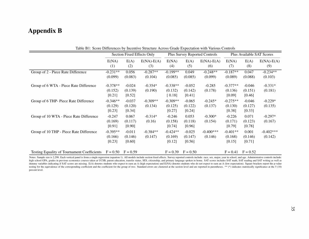
B1 reports the results for the main specification with varying levels of controls. The first panel
includes only section fixed effects, the second panel adds survey reported controls (the specification
reported in Table 3), and the third panel further adds the available administrative controls. As
6In an unreported analysis, we check for “giving-up” behavior. There is no evidence suggesting students answermore correct questions in the first half of the quiz relative to the last part.
12
expected, the results are similar across all specifications.
As there is no evidence that tournament size or payment structure matters, we simplify all
subsequent analysis by collapsing all tournament treatments into a single “compete” category and
report all results relative to the piece rate treatment. To facilitate comparison across tables, Table
4 repeats the Table 3 analysis using this averaged specification. Column 1 of Table 4 shows that
the average score in a competitive treatment is 22.3 percent of a standard deviation lower than the
average piece rate score for low expectation students. Column 2 similarly shows that the average
score for high expectation students is 5.9 percent of a standard deviation higher compared to those
in the piece rate treatment, but this point estimate is not statistically significant at conventional
levels.7
These results naturally lead one to wonder whether expected grades reflect actual ability/skill
or over/under confidence of some type for some subgroups. Our administrative data on grades in
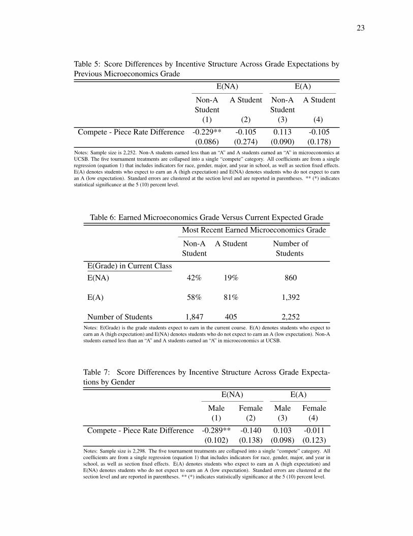
core economics courses allow us to probe this issue. Table 5 interacts expected grade with earned
grade, where earned grade is defined as the participant’s first intermediate microeconomics grade.
If no intermediate theory grade is available, we use their principles grade. The sample size is
slightly smaller for this table because we have no grades for foreign exchange students and a small
number of students who enrolled as junior college transfers before the first intermediate theory
course was moved into the pre-major. We divide students into two groups: those who earn less
than an “A” (non-A students) and those who earn an “A” (A students).
Not surprisingly, as we sub-sample or interact to greater degrees, many estimates become quite
noisy. What is clear, is that the subset of subjects who are non-A students who also have low
expectations put forth less effort when assigned to competitive treatments (column 1), and this
competition effect is statistically different from the competition effect for high expectation non-A
students (compare columns 1 and 3). In summary, we can rule out large negative effects for non-
A students with high expectation suggesting that optimism or overconfidence shields this group
from the negative competition effect. And, while the other comparisons are noisy (i.e, comparing
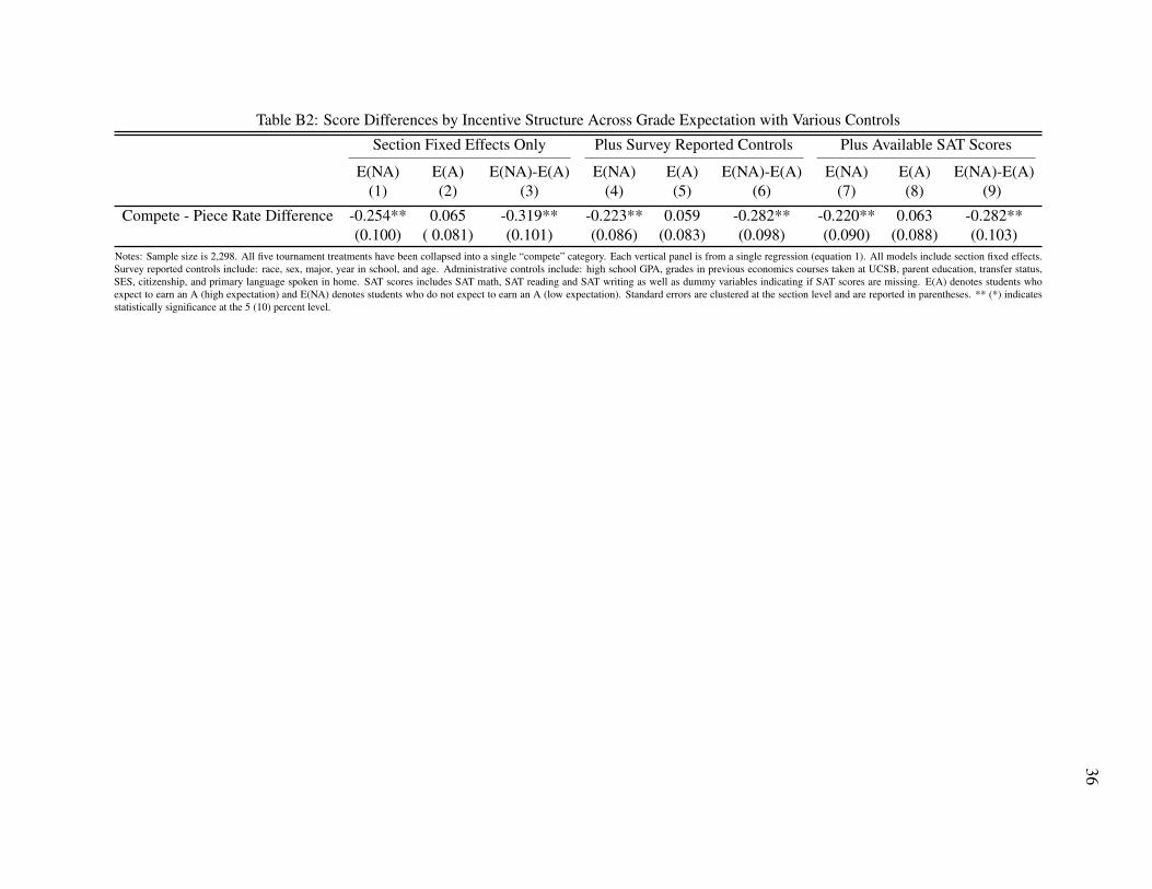
7Appendix Table B2 reports the results for this specification with varying levels of controls. The results are similaracross all specifications.

13
columns 1 and 2), what we can say with some confidence is that reduced effort when confronted
with competition seems to be driven by weaker students who realize that they are weaker students,
a result that is more consistent with honest self-reflection than under confidence.
At least part of the reason that the low expectation non-A student group is driving the results is
because this is where the discrepancy between earned and expected grades exists. Table 6 shows
that among A students, about 81 percent expect to earn an “A” in the current course. On the other
hand, among non-A students, 42 percent expect less than an “A” and 58 percent expect an “A”.8
Many previous studies identify important differences in effort response to competition by gen-
der. In a variety of field and lab settings, it has been shown that men tend to increase their effort
when forced to compete, while women’s performance is unchanged (Gneezy et al., 2003; Gneezy
and Rustichini, 2004). Table 7 replicates Table 5 but instead of earned grade, we interact expected
grade with gender. Columns 1 and 2 (3 and 4) report the competition effect for low (high) expecta-
tion men and women. In contrast to previous studies, in our setting the negative competition effect
point estimate is most negative for low expectation men, but due to imprecision, we cannot reject
that the male and female effects are the same for students within expectation groups. Overall, these
findings are consistent, but not definitive, evidence that the competition effects are driven by less
able men exerting less effort when forced to compete.9
5.2 Task Type
In contrast to many previous studies, in our setting we find that competition reduces effort, at
least for an important subset of participants. In this section we investigate two possible features
of our experiment that might explain the divergence of our results from past findings that show
performance improves, at least among some sub-groups, when subjects are forced to compete.
First, we explore the potential role of task type. In our design, subjects take a microeconomics
quiz. Relative to the tasks that are often implemented, such as solving mazes or adding up two-
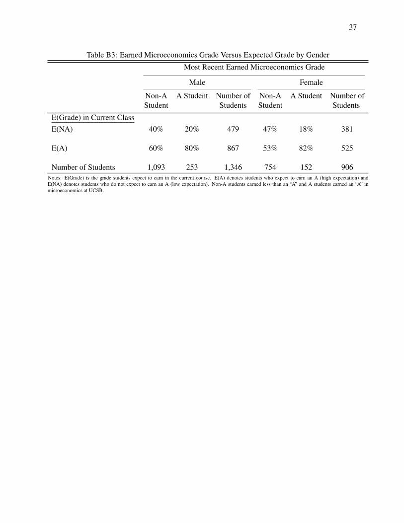
8Appendix Table B3 disaggregates Table 6 by gender.9In an unreported analysis, we find no evidence of gender differences in the response to the sex composition of the
group.
14
digit numbers, the task in this experiment draws on a more specialized skill. Second, our sample
is selected on major or course enrollment (largely economics and accounting students), but has
almost no selection on the showing up or signing up margin since all quizzes took place at the start
of sections and essentially 100 percent of students attending section participated. We examine each
of these in turn.
To test whether a specialized skill task in a competitive environment has a different effect on
performance than a more general skill task, we implement an additional treatment. In this treat-
ment students were asked to multiply and add sequences of numbers without a calculator. These
simple calculations were formatted to look like microeconomics questions because this treatment
was administered in the same sections as the microeconomics quiz task. For example, questions
from the more general skill task included calculating rent, minimum cost, and average return. For
simplicity, we only included one competitive incentive scheme, group of two (we call this com-
pete), and the piece rate treatment. Table 8 reports summary statistics for these additional rounds.
For comparative purposes, column 1 reports the average raw quiz score, the average standardized
score, the percent of the sample with high expectations, and the percent female for participants
assigned to the piece rate and group of two standard microeconomics quiz treatments. Column 2
reports the same summary measures for participants assigned to the general skill task, again in-
cluding both piece rate and groups of two. It is important to note that you cannot compare the
average raw scores across columns 1 and 2 because the tests are very different.
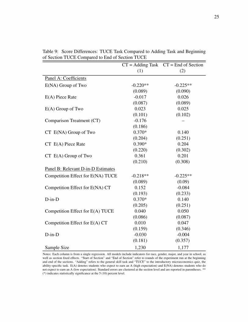
We use an empirical specification similar to equation 1. The primary differences are as follows.
First, there are only two compensation schemes: compete and piece rate (piece rate for low expec-
tation students continues to be the omitted category). Second, the model now includes an indicator
variable for the general skill task and this indicator is interacted with the three treatment group
indicators (low expectation compete, high expectation piece rate, and high expectation compete).
Column 1 of Table 9 reports the results. As in the main results reported in Table 4, low expec-
tation participants exert less effort on the microeconomics quiz when forced to compete, while
the effort of high expectation students does not change (see Panel B). Low expectation students

15
score 22.0 percent of a standard deviation lower in the group of two treatment compared to the
piece rate treatment. In contrast, low expectation students assigned to the adding/multiplying task
score higher when assigned to the competitive treatment, although the point estimate is noisy. The
difference-in-difference estimate shows that the competition effect for the general skill task is 37.0
of a standard deviation higher than the competition effect for the specialized skill task. Even if the
competition effect for the general skill task is indistinguishable from zero, we can reject that it is
as negative as the competition effect for the specialized skill task for the low expectation group.
Taken together, these results suggest that effort in competitive environments depends importantly
on the nature of the task. And if the task involves a specialized skill, it also depends on ability.
Unsurprising, our general skill treatment yields results similar to what has previously been found
in the experimental literature, as those studies implement tasks involving similar skills. Results for
the microeconomics quiz task are quite different.
5.3 Selection into Participation
In order to explore the potential for at least some forms of selection to impact the results, we ran
11 additional sessions in which we allowed, even encouraged, more selection into participation.
In contrast to all other sessions, these sessions were run at the end sections. Students were invited
to stay and take the microeconomics quiz under the same set of incentives as before. On average,
approximately half of the students present chose to participate (compared to essentially 100 per-
cent in the beginning of section sessions). Summary statistics for these additional end of section
sessions are reported in last column of Table 8. There is some evidence of selection; stayers score
slightly better on average and are somewhat more likely to be male. Of course, our primary ques-
tion is whether this selection implies a different response for those who are randomly assigned to
compete.
The results are reported in column 2 of Table 9. The specification is identical to that explor-
ing the difference between the microeconomics quiz task and the general skill quiz in column 1,
except that the indicator for the new treatment (the end of section treatment) cannot be identified
16
separately from section fixed effects. We can, however, identify this indicator interacted with the
three included treatment group indicators (low expectation compete, high expectation piece rate,
and high expectation compete). In contrast to the differential response to competition in special-
ized and general skill tasks, the response to competition in sessions run at the beginning of section
and at the end of section (less and more selected participation cases) are both negative for low ex-
pectation students, and we cannot reject the null hypothesis that the point estimates are the same.
And as in all other cases, there is no evidence of an effort response for high expectation students.
The end of session results suggest that the reason our main findings differ from previous studies is
not our use of a less selected sample, but rather stems from the difference in task type.
6 Conclusion
In a classroom setting where students are asked to complete a real-effort task, we show that indi-
viduals who believe they are lower scoring students reduce their effort when forced to compete,
while there are few detectable effects for students who expect to earn higher grades. We find that
students who believe they will earn less than an “A” grade in their current economics course score
about 22 percent of a standard deviation lower when forced to compete compared to the piece rate
treatment, and that this effect is driven by men and low expectation students who have realistic
beliefs about their ability. In contrast, previous research has tended to find that men increase their
effort level when forced to compete. Perhaps the biggest take away from this experiment is the ev-
idence that our results diverge from past findings because of task type differences and not because
of selection. The evidence clearly suggests that task type plays a critical role in one’s response to
competition. Stated more generally, responses to competition are likely to depend importantly on
the environment and the individual’s position in the skill distribution; people who might increase
their effort when faced with competition in one environment might decrease or not change their
effort in another environment. As such, one should be cautious, perhaps even skeptical, about
generalizing results about the distribution of responses to competition from one context to another.
17
References
Andreoni, James and Andy Brownback, “Grading on a Curve, and Other Effects of Group Sizeon All-Pay Auctions,” Technical Report, National Bureau of Economic Research 2014.
Barut, Yasar, Dan Kovenock, and Charles N Noussair, “A Comparison of Multiple-Unit All-Pay and Winner-Pay Auctions Under Incomplete Information,” International Economic Review,2002, 43 (3), 675–708.
Becker, William E and Sherwin Rosen, “The Learning Effect of Assessment and Evaluation inHigh School,” Economics of Education Review, 1992, 11 (2), 107–118.
Beyer, Sylvia, “Gender Differences in the Accuracy of Self-evaluations of Performance.,” Journalof Personality and Social Psychology, 1990, 59 (5), 960.
Booth, Alison and Patrick Nolen, “Choosing to Compete: How Different are Girls and Boys?,”Journal of Economic Behavior & Organization, 2012, 81 (2), 542–555.
Booth, Alison L and Patrick Nolen, “Gender Differences in Risk Behaviour: Does Nurture Mat-ter?,” The Economic Journal, 2012, 122 (558), F56–F78.
Brown, Jennifer, “Quitters Never Win: The (Adverse) Incentive Effects of Competing with Su-perstars,” Journal of Political Economy, 2011, 119 (5), 982–1013.
Bull, Clive, Andrew Schotter, and Keith Weigelt, “Tournaments and Piece Rates: An Experi-mental Study,” Journal of Political Economy, 1987, 95 (1), 1–33.
Cárdenas, Juan-Camilo, Anna Dreber, Emma Von Essen, and Eva Ranehill, “Gender Dif-ferences in Competitiveness and Risk Taking: Comparing Children in Colombia and Sweden,”Journal of Economic Behavior & Organization, 2012, 83 (1), 11–23.
Chemers, Martin M, Li tze Hu, and Ben F Garcia, “Academic Self-Efficacy and First YearCollege Student Performance and Adjustment.,” Journal of Educational Psychology, 2001, 93(1), 55.
Dohmen, Thomas and Armin Falk, “Performance Pay and Multidimensional Sorting: Produc-tivity, Preferences, and Gender,” The American Economic Review, 2011, pp. 556–590.
Dreber, Anna, Emma von Essen, and Eva Ranehill, “Gender and competition in adolescence:task matters,” Experimental Economics, 2014, 17 (1), 154–172.
Eckel, Catherine C and Philip J Grossman, “Men, Women and Risk Aversion: ExperimentalEvidence,” Handbook of Experimental Economics Results, 2008, 1, 1061–1073.
Garratt, Rodney J, Catherine Weinberger, and Nick Johnson, “The State Street Mile: Ageand Gender Differences in Competition Aversion in the Field,” Economic Inquiry, 2013, 51 (1),806–815.

18
Gillen, Ben, Erik Snowberg, and Leeat Yariv, “Experimenting with Measurement Error: Tech-niques with Applications to the Caltech Cohort Study,” Technical Report, National Bureau ofEconomic Research 2015.
Gneezy, Uri and Aldo Rustichini, “Gender and Competition at a Young Age,” American Eco-nomic Review Papers and Proceedings, 2004, pp. 377–381.
, Kenneth L Leonard, and John A List, “Gender Differences in Competition: Evidence froma Matrilineal and a Patriarchal Society,” Technical Report 2009.
, Muriel Niederle, and Aldo Rustichini, “Performance in Competitive Environments: GenderDifferences,” Quarterly Journal of Economics, 2003, 118 (3), 1049–1074.
Green, Jerry R and Nancy L Stokey, “A Comparison of Tournaments and Contracts,” Journal ofPolitical Economy, 1983, pp. 349–364.
Günther, Christina, Neslihan Arslan Ekinci, Christiane Schwieren, and Martin Strobel,“Women Can’t Jump? - An experiment on competitive attitudes and stereotype threat,” Jour-nal of Economic Behavior & Organization, 2010, 75 (3), 395–401.
Gupta, Nabanita Datta, Anders Poulsen, and Marie Claire Villeval, “Gender Matching andCompetitiveness: Experimental Evidence,” Economic Inquiry, 2013, 51 (1), 816–835.
Harbring, Christine and Bernd Irlenbusch, “An Experimental Study on Tournament Design,”Labour Economics, 2003, 10 (4), 443–464.
Kagel, John H and Alvin E Roth, The Handbook of Experimental Economics, Princeton Univer-sity Press Princeton, NJ, 1995.
Kuhn, Peter and Marie Claire Villeval, “Are Women More Attracted to Co-operation ThanMen?,” The Economic Journal, 2015, 125 (582), 115–140.
Lazear, Edward P and Sherwin Rosen, “Rank-Order Tournaments as Optimum Labor Con-tracts,” 1981.
Lima, Wooyoung, Alexander Matros, and Theodore Turocy, “Bounded Rationality and GroupSize in Tullock Contests: Experimental Evidence,” Journal of Economic Behavior & Organiza-tion, 2014, 99, 155–167.
List, John, Daan Van Soest, Jan Stoop, and Haiwen Zhou, “On the Role of Group Size in Tour-naments: Theory and Evidence from Lab and Field Experiments,” Technical Report, NationalBureau of Economic Research 2014.
Moore, Don A and Deborah A Small, “Error and Bias in Comparative Judgment: On BeingBoth Better and Worse Than We Think We Are.,” Journal of Personality and Social Psychology,2007, 92 (6), 972.
Nalbantian, Haig R and Andrew Schotter, “Productivity Under Group Incentives: An Experi-mental Study,” American Economic Review, 1997, pp. 314–341.
19
Niederle, Muriel and Alexandra H Yestrumskas, “Gender Differences in Seeking Challenges:The Role of Institutions,” Technical Report, National Bureau of Economic Research 2008.
and Lise Vesterlund, “Do Women Shy Away from Competition? Do Men Compete TooMuch?,” Quarterly Journal of Economics, 2007, 122, 1067–1101.
Orrison, Alannah, Andrew Schotter, and Keith Weigelt, “Multiperson Tournaments: An Ex-perimental Examination,” Management Science, 2004, 50 (2), 268–279.
Prendergast, Canice, “The Provision of Incentives in Firms,” Journal of Economic Literature,1999, 37 (1), 7–63.
Sutter, Matthias and Daniela Rutzler, “Gender Differences in Competition Emerge Early inLife,” 2015.
Villeval, Marie Claire, “Ready, Steady, Compete,” Science, 2012, 335 (3), 544–545.
Zizzo, Daniel John, “Experimenter Eemand Effects in Economic Experiments,” ExperimentalEconomics, 2010, 13 (1), 75–98.

20
Table 1: Summary Statistics - Test Scores (TUCE) and Expected Grades
Score Standardized E(A) Sample SizeScore
(1) (2) (3) (4)
Panel A: Treatment Group
Piece rate 5.49 0.01 0.57 417(2.03) (0.98) (0.50)
Group of Two 5.14 0.02 0.60 641(2.06) (0.99) (0.49)
Group of Six WTA 5.10 0.02 0.64 309(1.91) (0.93) (0.48)
Group of Six THP 4.76 -0.04 0.64 311(1.90) (0.92) (0.48)
Group of Ten WTA 4.81 0.03 0.65 321(1.99) (1.01) (0.48)
Group of Ten THP 5.17 -0.01 0.64 299(2.06) (1.05) (0.48)
Panel B: GenderMale 5.36 0.12 0.64 1,376
(2.02) (0.99) (0.48)Female 4.73 -0.15 0.58 922
(1.96) ( 0.94) (0.49)Panel C: Class Standing
Lower Division 4.84 0.000 0.61 1,678(1.97) (0.99) (0.49)
Upper Division 5.81 0.04 0.64 620(1.97) (0.99) (0.49)
Notes: Mean scores and expected grades are reported by subgroups. Standard deviations are in parentheses. E(A)denotes students who expect to earn an A (high expectation) and E(NA) denotes students who do not expect to earnan A (low expectation). WTA are treatments where the top scorer is paid, THP are treatments where the top half ofthe group is paid.
21
Table 2: Pre-Treatment Characteristics - Sample Balance
Differences Between Treatments
Group of 2 Piece Group of 6 Group of 6 Group of 10 Group of 10Mean Rate WTA THP WTA THP
(1) (2) (3) (4) (5) (6)
Panel A: E(NA)Female 0.41 -0.04 0.14 0.11 0.20 0.04
(0.49) [0.50] [0.06] [0.17] [0.03] [0.65]Hispanic 0.18 0.06 -0.09 0.04 0.08 -0.10
(0.39) [0.23] [0.12] [0.47] [0.27] [0.15]Black 0.02 -0.01 0.04 0.00 0.00 0.04
(0.12) [0.60] [0.06] [0.96] [0.94] [0.12]Asian 0.37 -0.09 0.02 -0.09 -0.05 0.03
(0.48) [0.18] [0.78] [0.25] [0.57] [0.71]Other 0.07 -0.01 -0.03 -0.04 -0.06 -0.03
(0.26) [0.70] [0.45] [0.32] [0.20] [0.42]Accounting Major 0.42 0.09 0.03 -0.05 -0.05 -0.15
(0.49) [0.14] [0.70] [0.50] [0.55] [0.06]Other Major 0.30 -0.09 0.01 0.09 0.10 0.07
(0.46) [0.07] [0.83] [0.12] [0.14] [0.31]Sophomore 0.30 0.11 -0.11 0.11 0.15 -0.04
(0.46) [0.03] [0.06] [0.10] [0.06] [0.57]Junior 0.36 -0.07 0.11 0.06 0.01 0.06
(0.48) [0.22] [0.06] [0.38] [0.88] [0.39]Senior 0.19 0.00 -0.09 -0.04 -0.05 -0.10
(0.39) [0.95] [0.02] [0.29] [0.21] [0.04]Age 20-21 0.38 0.05 0.05 0.08 0.05 -0.04
(0.49) [0.45] [0.47] [0.24] [0.49] [0.58]Age 22+ 0.17 -0.04 -0.05 -0.05 -0.07 0.00
(0.37) [0.39] [0.35] [0.37] [0.23] [0.96]Sample Size 256 437 367 369 367 364
Panel B: E(A)Female 0.39 -0.08 0.02 -0.08 0.03 0.02
(0.49) [0.13] [0.69] [0.15] [0.63] [0.77]Hispanic 0.14 -0.02 0.06 -0.06 -0.04 0.03
(0.35) [0.52] [0.14] [0.13] [0.32] [0.52]Black 0.02 0.00 0.00 0.01 0.00 -0.02
(0.13) [0.88] [0.83] [0.54] [0.73] [0.24]Asian 0.45 0.00 0.00 0.04 0.01 -0.01
(0.50) [0.95] [0.95] [0.47] [0.93] [0.90]Other 0.05 -0.03 0.01 0.01 0.02 0.02
(0.21) [0.20] [0.64] [0.66] [0.51] [0.63]Accounting Major 0.42 -0.01 -0.07 0.04 0.00 0.08
(0.50) [0.84] [0.21] [0.45] [0.99] [0.17]Other Major 0.29 0.08 0.06 -0.04 -0.06 -0.04
(0.46) [0.05] [0.19] [0.33] [0.09] [0.41]Sophomore 0.27 -0.05 -0.05 -0.04 0.03 0.01
(0.45) [0.24] [0.24] [0.38] [0.58] [0.90]Junior 0.39 0.04 0.03 0.02 -0.10 0.02
(0.49) [0.43] [0.52] [0.73] [0.04] [0.78]Senior 0.19 0.03 -0.04 -0.02 0.04 -0.04
(0.39) [0.34] [0.18] [0.60] [0.29] [0.36]Age 20-21 .39 0.06 0.11 -0.02 -0.11 0.06
(0.49) [0.29] [0.04] [0.68] [0.05] [0.36]Age 22+ 0.22 0.01 -0.11 -0.01 0.02 -0.10
(0.42) [0.84] [0.01] [0.72] [0.69] [0.06]Sample Size 385 621 583 583 595 576
Notes: Column 1 reports means for the group of two treatment. Corresponding standard deviations are in parentheses. Differences in columns 2-6 arefrom OLS regressions that include section fixed effects. Sample sizes listed in columns 2-6 include the group of two and the group listed at the top ofeach column. P-values for differences are in square brackets. E(A) denotes students who expect to earn an A (high expectation) and E(NA) denotesstudents who do not expect to earn an A (low expectation). WTA are treatments where the top scorer is paid, THP are treatments where the top halfof the group is paid.
22
Table 3: Score Differences by Incentive Structure Across Grade Expectation
Difference Estimates Effects StatisticallyDifferent?
E(NA) E(A) (1)-(2)(1) (2) (3)
Group of 2 - Piece Rate Difference -0.199** 0.049 -0.248**(0.085) (0.085) (0.099)
Group of 6 WTA - Piece Rate Difference -0.338** -0.052 -0.285(0.132) (0.142) (0.178)[ 0.18] [0.41]
Group of 6 THP - Piece Rate Difference -0.309** -0.065 -0.245*(0.125) (0.122) (0.137)[0.27] [0.24]
Group of 10 WTA - Piece Rate Difference -0.246 0.053 -0.300*(0.158) (0.118) (0.154)[0.74] [0.96]
Group of 10 THP - Piece Rate Difference -0.424** -0.025 -0.400**(0.169) (0.147) (0.146)[0.12] [0.56]
Testing Equality of Tournament Coefficients F = 0.39 F = 0.50Notes: Sample size is 2,298. All coefficients are from a single regression (equation 1) that includes indicators for race, gender, major,and year in school, as well as section fixed effects. E(A) denotes students who expect to earn an A (high expectation) and E(NA) denotesstudents who do not expect to earn an A (low expectation). WTA are treatments where the top scorer is paid and THP are treatments wherethe top half of the group is paid. Standard errors are clustered at the section level and are reported in parentheses. Square brackets reportthe p-value testing for the equivalence of the corresponding coefficient and the coefficient for the group of two. ** (*) indicates statisticalsignificance at the 5 (10) percent level.
Table 4: Score Differences by Incentive Structure Across Grade Expectation
Difference Estimates Effects StatisticallyDifferent?
E(NA) E(A) (1)-(2)(1) (2) (3)
Compete - Piece Rate Difference -0.223** 0.059 -0.282**(0.086) (0.083) (0.098)
Notes: Sample size is 2,298. The five tournament treatments are collapsed into a single “compete” category. All coeffi-cients are from a single regression (equation 1) that includes indicators for race, gender, major, and year in school, as wellas section fixed effects. E(A) denotes students who expect to earn an A (high expectation) and E(NA) denotes studentswho do not expect to earn an A (low expectation). Standard errors are clustered at the section level and are reported inparentheses. ** (*) indicates statistical significance at the 5 (10) percent level.
23
Table 5: Score Differences by Incentive Structure Across Grade Expectations byPrevious Microeconomics Grade
E(NA) E(A)
Non-A A Student Non-A A StudentStudent Student
(1) (2) (3) (4)
Compete - Piece Rate Difference -0.229** -0.105 0.113 -0.105(0.086) (0.274) (0.090) (0.178)
Notes: Sample size is 2,252. Non-A students earned less than an “A” and A students earned an “A” in microeconomics atUCSB. The five tournament treatments are collapsed into a single “compete” category. All coefficients are from a singleregression (equation 1) that includes indicators for race, gender, major, and year in school, as well as section fixed effects.E(A) denotes students who expect to earn an A (high expectation) and E(NA) denotes students who do not expect to earnan A (low expectation). Standard errors are clustered at the section level and are reported in parentheses. ** (*) indicatesstatistical significance at the 5 (10) percent level.
Table 6: Earned Microeconomics Grade Versus Current Expected Grade
Most Recent Earned Microeconomics Grade
Non-A A Student Number ofStudent Students
E(Grade) in Current ClassE(NA) 42% 19% 860
E(A) 58% 81% 1,392
Number of Students 1,847 405 2,252Notes: E(Grade) is the grade students expect to earn in the current course. E(A) denotes students who expect toearn an A (high expectation) and E(NA) denotes students who do not expect to earn an A (low expectation). Non-Astudents earned less than an “A” and A students earned an “A” in microeconomics at UCSB.
Table 7: Score Differences by Incentive Structure Across Grade Expecta-tions by Gender
E(NA) E(A)
Male Female Male Female(1) (2) (3) (4)
Compete - Piece Rate Difference -0.289** -0.140 0.103 -0.011(0.102) (0.138) (0.098) (0.123)
Notes: Sample size is 2,298. The five tournament treatments are collapsed into a single “compete” category. Allcoefficients are from a single regression (equation 1) that includes indicators for race, gender, major, and year inschool, as well as section fixed effects. E(A) denotes students who expect to earn an A (high expectation) andE(NA) denotes students who do not expect to earn an A (low expectation). Standard errors are clustered at thesection level and are reported in parentheses. ** (*) indicates statistically significance at the 5 (10) percent level.

24
Table 8: Summary Statistics for Mechanism Exploration Rounds
Start of Section Start of Section End of SectionTask=TUCE Task=Adding Task=TUCE
(1) (2) (3)
Score 5.28 7.20 5.97(2.06) (2.05) (1.89)
Standardized Score 0.02 0.00 0.12(0.99) (0.97) (0.83)
E(A) 0.59 0.56 0.55(0.49) (0.50) (0.50)
Female 0.40 0.46 0.34(0.49) (0.50) (0.47)
Sample Size 1,058 172 119Notes: Means are reported by subgroup. Standard deviations are in parentheses. “Start of Section” and “End ofSection” refer to rounds of the experiment run at the beginning and end of the sections. “Adding” refers to thegeneral skill task and “TUCE” to the introductory microeconomics quiz, the ability-specific task. E(A) denotesstudents who expect to earn an A (high expectation).
25
Table 9: Score Differences: TUCE Task Compared to Adding Task and Beginningof Section TUCE Compared to End of Section TUCE
CT = Adding Task CT = End of Section(1) (2)
Panel A: CoefficientsE(NA) Group of Two -0.220** -0.225**
(0.089) (0.090)E(A) Piece Rate -0.017 0.026
(0.087) (0.089)E(A) Group of Two 0.023 0.025
(0.101) (0.102)Comparison Treatment (CT) -0.176 –
(0.186)CT E(NA) Group of Two 0.370* 0.140
(0.204) (0.251)CT E(A) Piece Rate 0.390* 0.204
(0.220) (0.302)CT E(A) Group of Two 0.361 0.201
(0.210) (0.308)Panel B: Relevant D-in-D EstimatesCompetition Effect for E(NA) TUCE -0.218** -0.225**
(0.089) (0.09)Competition Effect for E(NA) CT 0.152 -0.084
(0.193) (0.233)D-in-D 0.370* 0.140
(0.205) (0.251)Competition Effect for E(A) TUCE 0.040 0.050
(0.086) (0.087)Competition Effect for E(A) CT 0.010 0.047
(0.159) (0.346)D-in-D -0.030 -0.004
(0.181) (0.357)Sample Size 1,230 1,177
Notes: Each column is from a single regression. All models include indicators for race, gender, major, and year in school, aswell as section fixed effects. “Start of Section” and “End of Section” refer to rounds of the experiment run at the beginningand end of the sections. “Adding” refers to the general skill task and “TUCE” to the introductory microeconomics quiz, theability-specific task. E(A) denotes students who expect to earn an A (high expectation) and E(NA) denotes students who donot expect to earn an A (low expectation). Standard errors are clustered at the section level and are reported in parentheses. **(*) indicates statistically significance at the 5 (10) percent level.

26
Appendix A

27
Entry Survey
You are being asked to participate in a study by Kelly Bedard, Stefanie Fischer, and Jon Sonstelie. For your participation today, we will enter you in a lottery in which one person in this class will receive $25 cash today (photo ID required). If you are younger than 18 you are not eligible for the lottery. While those under 18 years of age can participate in the tournament, your data will not be used for research purposes. You have also been selected to receive the opportunity to compete against the person with the same color quiz sitting near you. The highest scoring person in your pair will win $1 for each of their correct answers. The microeconomics quiz includes 10 randomly selected questions. You have 15 minutes to complete the quiz. In the event of a tie, you will split the prize equally. All participants will be notified by email when scores are posted on Gauchospace. Winners will also be notified by email about the date of payment. All payments will be made outside the classroom at the end of class on the specified date. Winners will be paid in approximately ten days. We are conducting a study to assess proficiency in foundational microeconomics and analyze competition and test taking. By signing up for this experiment, you are acknowledging that the authors of this study will follow your academic records at UCSB from the beginning of your enrollment through summer 2014. This data will not be used for any other purpose nor will any information ever be made public. All identifying data will be held in confidence from all instructors until after this academic quarter. That being said, absolute confidentiality cannot be guaranteed, since research documents are not protected from subpoena. Your participation is voluntary. There will be no repercussions should you decide not to participate. You may withdraw your participation at any time and remain eligible for the $25 lottery. If you have questions you may contact Kelly Bedard at [email protected] or 805‐893‐5571 or the University of California Santa Barbara Human Subjects committee at 805‐893‐3807. By signing below, you acknowledge the above information. We would like to ask you a few questions: What is your sex? (A) Female (B) Male How old are you? (A) 17 (B) 18 or 19 (C) 20 or 21 (D) 22 or 23 (E) 24+ Are you Hispanic/Latino? (A) Yes (B) No What is your race? (A) White (B) Black (C) Asian (D) Other Academic Year? (A) Freshman (B) Sophomore (C) Junior (D) Senior Major/Intended Major? (A) Economics (B) Economics & (C) Economics & (D) Other (E) Undecided Accounting Mathematics _____________________________________ ____________________________________ Print name Signature _____________________________________ ____________________________________ Date Perm # _____________________________________ ____________________________________ Primary e‐mail address Local phone number

28
Form 1 of the TUCE Quiz (Specialized Skill Task)
8. Suppose a city facing a shortage of rental apartments eliminates rent controls. Which of the
following is most likely to occur?
A. a decrease in rents and a decrease in the number of apartment units supplied
B. an increase in rents and an increase in the number of apartment units supplied C. a decrease in the demand for apartments and an increase in the number of apartment
units supplied D. an increase in the demand for apartments and a decrease in the number of apartment
units supplied
9. If all of the firms in a competitive industry are legally required to meet new regulations that
increase their cost of production:
A. supply of the product will decrease. B. demand for the product will decrease. C. the long‐run economic profits of individual firms in the industry will decrease. D. the short‐run economic profits of individual firms in the industry will increase.
10. At the profit‐maximizing level of output, a perfectly competitive firm will:
A. produce the quantity of output at which marginal cost equals price. B. produce the quantity of output at which marginal cost is minimized.
C. keep marginal cost lower than price, so profits will be greater than zero.
D. try to sell all the output it can produce, to spread fixed costs across the largest possible number of units.
11. A state legislature increased the tax on gasoline sold in the state from $.20 to $.30 per
gallon. A supporter said the tax would "make the distribution of after‐tax income in the
state more equal." This statement would be true only if it could be shown that, after the
tax is increased:
A. people with low incomes buy more gasoline than people with high incomes. B. the quantity of gasoline purchased in the state is highly responsive to changes in price. C. people with high incomes tend to spend the same proportion of their incomes on gasoline
as people with low incomes. D. people with high incomes tend to spend a larger proportion of their incomes on gasoline
than people with low income.
12. The opportunity cost of being a full‐time student at a university instead of working full‐
time at a job includes all of the following EXCEPT:
A. payments for meals.
B. payments for tuition.
C. payments for books.
D. income from the full‐time job.

29
13. "Water is essential to life, but inexpensive to buy." Which of the following best explains this
observation?
A. Water has a high total utility, but a low marginal utility.
B. Water has a low total utility, but a high marginal utility.
C. The quantity supplied of water is less than the quantity demanded at the market price.
D. The quantity supplied of water is greater than the quantity demanded at the market
price.
14. Which of the following is true for this profit‐maximizing firm at price P in the graph
above?
A. It is not earning any economic profits.
B. It is currently earning short‐run economic profits.
C. It should shut down to minimize its economic losses.
D. It will continue to earn economic profits in the long run.
15. If the exchange rate between dollars ($) and yen (¥) changes from $1 = ¥200 to $1 =
¥100, and domestic prices in both countries stay the same, has the dollar appreciated or
depreciated, and would U.S. imports from Japan become less expensive or more expensive?
Value of the dollar U.S. imports from Japan
A. Appreciated Less expensive
B. Appreciated More expensive
C. Depreciated Less expensive
D. Depreciated More expensive
30
16. Suppose the only two cola companies (Acola and Bcola) in a nation are deciding whether to
charge high or low prices for their colas. The companies' price strategies are shown in the
table below. The four pairs of payoff values show what each company expects to earn or lose
in millions of dollars, depending on what the other company does.
Acola’s Price Strategy
High Price Low Price
Bcola’s Price Strategy
High Price Acola +$100
Bcola +$100
Acola +$250
Bcola ‐$50
Low Price Acola ‐$50
Bcola +$250
Acola +$50
Bcola +$50
If both companies believe that most consumers are soon going to quit drinking colas, and
switch to other products, what is the equilibrium outcome?
A. Both Acola and Bcola will charge a low price.
B. Both Acola and Bcola will charge a high price.
C. Acola will charge‐a low price; Bcola will charge a high price.
D. Acola will charge a high price; Bcola will charge a low price.
17. In Sunshine City, one local ice cream company operates in a competitive labor market and
product market. It can hire workers for $45 a day and sell ice cream cones for $1.00 each.
The table below shows the relationship between the number of workers hired and the
number of ice cream cones produced and sold.
Number of Number of Ice
Workers Hired Cream Cones Sold
4 340
5 400
6 450
7 490
8 520
As long as the company stays in business, how many workers will it hire to maximize profits
or minimize losses?
A. 5 B. 6 C. 7 D. 8
31
Form 1 of the Adding/Multiplying Quiz (General Skill Task)
8. The owner of a company must choose between four money schemes. For each scheme, the owner of the firm gets the specified amount. Which scheme has the highest average payout? Hint: to answer this question you’ll need to calculate the average for each Scheme ‐‐ i.e. to find the average of Scheme 1 you would want to calculate (8+12+4+24)/4.
Scheme 1 Scheme 2 Scheme 3 Scheme 4
8 4 12 16
12 40 20 16
4 4 4 6
24 12 20 18
A. Scheme 1
B. Scheme 2 C. Scheme 3 D. Scheme 4
9. A real estate developer has to choose between four apartment buildings. Each building has four types of apartments which charge specific levels of rent. Which building generates the highest revenue (total rent)?
Rent Building 1 Building 2 Building 3 Building 4
1000 2 4 8 4
1500 4 2 4 6
2000 8 6 2 6
2500 2 4 4 2
A. Building 1
B. Building 2 C. Building 3 D. Building 4
10. A factory owner must upgrade his factory line. The factory line has five parts. He has bids from
four machine shops. Each bid includes all five parts. If the factory owner wants to pay the lowest cost possible for the upgrade, which bid should he choose?
Part Bid 1 Bid 2 Bid 3 Bid 4
Part 1 10,000 8,000 12,500 9,000
Part 2 12,000 14,000 8,000 11,000
Part 3 1,500 4,500 3,500 4,000
Part 4 2,000 3,000 3,000 4,000
Part 5 16,000 12,000 15,000 13,000
A. Bid 1
B. Bid 2 C. Bid 3 D. Bid 4
32
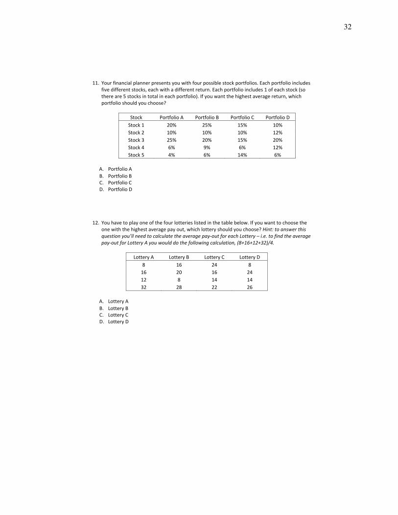
11. Your financial planner presents you with four possible stock portfolios. Each portfolio includes five different stocks, each with a different return. Each portfolio includes 1 of each stock (so there are 5 stocks in total in each portfolio). If you want the highest average return, which portfolio should you choose?
Stock Portfolio A Portfolio B Portfolio C Portfolio D
Stock 1 20% 25% 15% 10%
Stock 2 10% 10% 10% 12%
Stock 3 25% 20% 15% 20%
Stock 4 6% 9% 6% 12%
Stock 5 4% 6% 14% 6%
A. Portfolio A
B. Portfolio B C. Portfolio C D. Portfolio D
12. You have to play one of the four lotteries listed in the table below. If you want to choose the one with the highest average pay out, which lottery should you choose? Hint: to answer this question you’ll need to calculate the average pay‐out for each Lottery – i.e. to find the average pay‐out for Lottery A you would do the following calculation, (8+16+12+32)/4.
Lottery A Lottery B Lottery C Lottery D
8 16 24 8
16 20 16 24
12 8 14 14
32 28 22 26
A. Lottery A
B. Lottery B C. Lottery C D. Lottery D
33
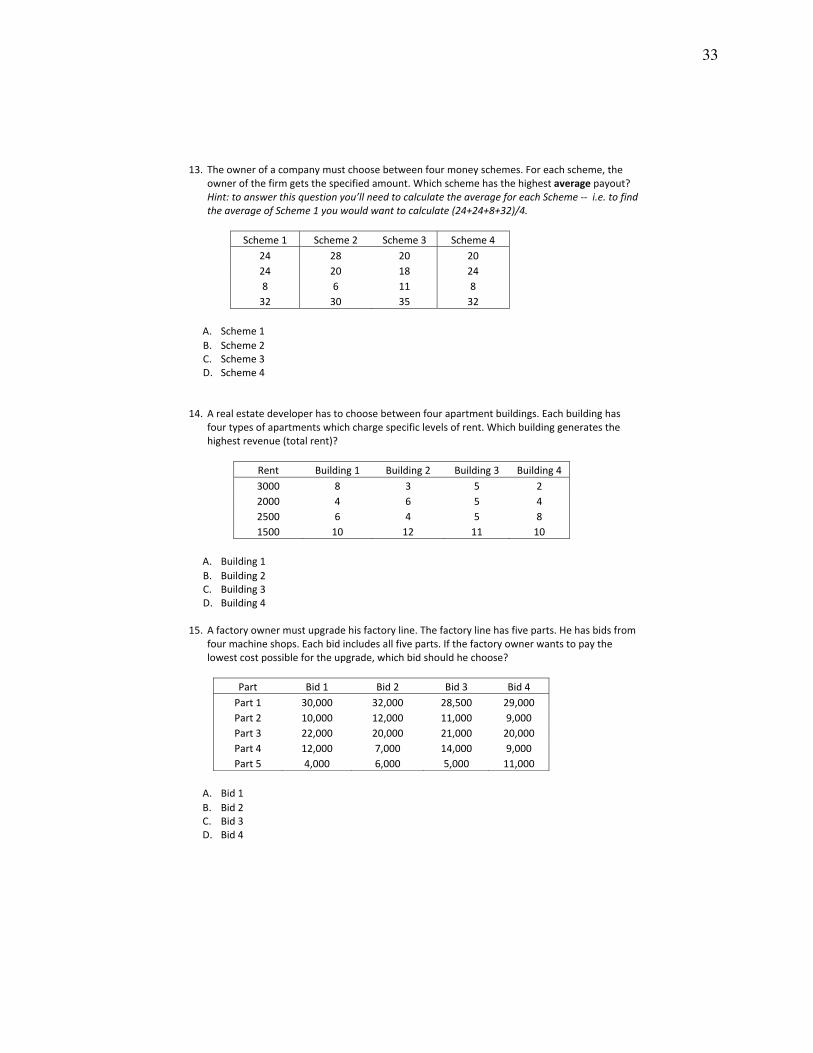
13. The owner of a company must choose between four money schemes. For each scheme, the owner of the firm gets the specified amount. Which scheme has the highest average payout? Hint: to answer this question you’ll need to calculate the average for each Scheme ‐‐ i.e. to find the average of Scheme 1 you would want to calculate (24+24+8+32)/4.
Scheme 1 Scheme 2 Scheme 3 Scheme 4
24 28 20 20
24 20 18 24
8 6 11 8
32 30 35 32
A. Scheme 1
B. Scheme 2 C. Scheme 3 D. Scheme 4
14. A real estate developer has to choose between four apartment buildings. Each building has four types of apartments which charge specific levels of rent. Which building generates the highest revenue (total rent)?
Rent Building 1 Building 2 Building 3 Building 4
3000 8 3 5 2
2000 4 6 5 4
2500 6 4 5 8
1500 10 12 11 10
A. Building 1
B. Building 2 C. Building 3 D. Building 4
15. A factory owner must upgrade his factory line. The factory line has five parts. He has bids from
four machine shops. Each bid includes all five parts. If the factory owner wants to pay the lowest cost possible for the upgrade, which bid should he choose?
Part Bid 1 Bid 2 Bid 3 Bid 4
Part 1 30,000 32,000 28,500 29,000
Part 2 10,000 12,000 11,000 9,000
Part 3 22,000 20,000 21,000 20,000
Part 4 12,000 7,000 14,000 9,000
Part 5 4,000 6,000 5,000 11,000
A. Bid 1
B. Bid 2 C. Bid 3 D. Bid 4
34
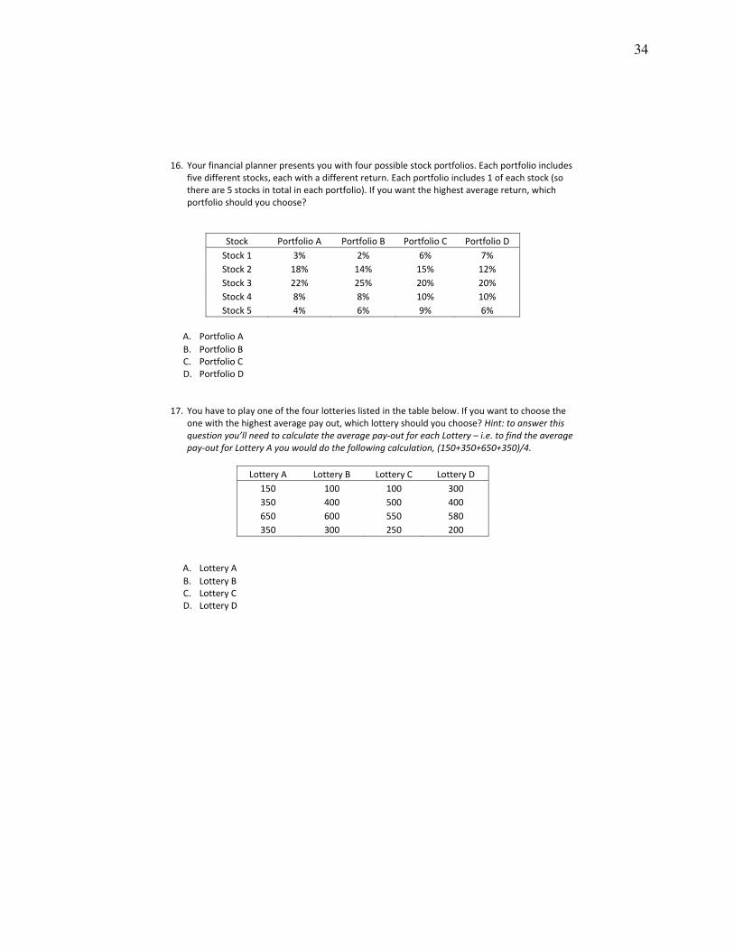
16. Your financial planner presents you with four possible stock portfolios. Each portfolio includes
five different stocks, each with a different return. Each portfolio includes 1 of each stock (so there are 5 stocks in total in each portfolio). If you want the highest average return, which portfolio should you choose?
Stock Portfolio A Portfolio B Portfolio C Portfolio D
Stock 1 3% 2% 6% 7%
Stock 2 18% 14% 15% 12%
Stock 3 22% 25% 20% 20%
Stock 4 8% 8% 10% 10%
Stock 5 4% 6% 9% 6%
A. Portfolio A
B. Portfolio B C. Portfolio C D. Portfolio D
17. You have to play one of the four lotteries listed in the table below. If you want to choose the one with the highest average pay out, which lottery should you choose? Hint: to answer this question you’ll need to calculate the average pay‐out for each Lottery – i.e. to find the average pay‐out for Lottery A you would do the following calculation, (150+350+650+350)/4.
Lottery A Lottery B Lottery C Lottery D
150 100 100 300
350 400 500 400
650 600 550 580
350 300 250 200
A. Lottery A
B. Lottery B C. Lottery C D. Lottery D
35
Appendix B
Table B1: Score Differences by Incentive Structure Across Grade Expectation with Various Controls
Section Fixed Effects Only Plus Survey Reported Controls Plus Available SAT Scores
E(NA) E(A) E(NA)-E(A) E(NA) E(A) E(NA)-E(A) E(NA) E(A) E(NA)-E(A)(1) (2) (3) (4) (5) (6) (7) (8) (9)
Group of 2 - Piece Rate Difference -0.231** 0.056 -0.287** -0.199** 0.049 -0.248** -0.187** 0.047 -0.234**(0.099) (0.083) (0.104) (0.085) (0.085) (0.099) (0.089) (0.088) (0.103)
Group of 6 WTA - Piece Rate Difference -0.378** -0.024 -0.354* -0.338** -0.052 -0.285 -0.377** -0.046 -0.331*(0.152) (0.139) (0.190) (0.132) (0.142) (0.178) (0.136) (0.151) (0.181)[0.21] [0.52] [ 0.18] [0.41] [0.09] [0.46]
Group of 6 THP- Piece Rate Difference -0.346** -0.037 -0.309** -0.309** -0.065 -0.245* -0.275** -0.046 -0.229*(0.129) (0.120) (0.134) (0.125) (0.122) (0.137) (0.130) (0.127) (0.135)[0.23] [0.34] [0.27] [0.24] [0.38] [0.33]
Group of 10 WTA - Piece Rate Difference -0.247 0.067 -0.314* -0.246 0.053 -0.300* -0.226 0.071 -0.297*(0.169) (0.117) (0.16) (0.158) (0.118) (0.154) (0.171) (0.123) (0.167)[0.91] [0.90] [0.74] [0.96] [0.79] [0.78]
Group of 10 THP - Piece Rate Difference -0.395** -0.011 -0.384** -0.424** -0.025 -0.400*** -0.401** 0.001 -0.402***(0.166) (0.146) (0.147) (0.169) (0.147) (0.146) (0.168) (0.146) (0.142)[0.23] [0.60] [0.12] [0.56] [0.15] [0.71]
Testing Equality of Tournament Coefficients F = 0.50 F = 0.59 F = 0.39 F = 0.50 F = 0.41 F = 0.52Notes: Sample size is 2,298. Each vertical panel is from a single regression (equation 1). All models include section fixed effects. Survey reported controls include: race, sex, major, year in school, and age. Administrative controls include:high school GPA, grades in previous economics courses taken at UCSB, parent education, transfer status, SES, citizenship, and primary language spoken in home. SAT scores includes SAT math, SAT reading and SAT writing as well asdummy variables indicating if SAT scores are missing. E(A) denotes students who expect to earn an A (high expectation) and E(NA) denotes students who do not expect to earn an A (low expectation). Square brackets report the p-valuetesting for the equivalence of the corresponding coefficient and the coefficient for the group of two. Standard errors are clustered at the section level and are reported in parentheses. ** (*) indicates statistically significance at the 5 (10)percent level.
36
Table B2: Score Differences by Incentive Structure Across Grade Expectation with Various Controls
Section Fixed Effects Only Plus Survey Reported Controls Plus Available SAT Scores
E(NA) E(A) E(NA)-E(A) E(NA) E(A) E(NA)-E(A) E(NA) E(A) E(NA)-E(A)(1) (2) (3) (4) (5) (6) (7) (8) (9)
Compete - Piece Rate Difference -0.254** 0.065 -0.319** -0.223** 0.059 -0.282** -0.220** 0.063 -0.282**(0.100) ( 0.081) (0.101) (0.086) (0.083) (0.098) (0.090) (0.088) (0.103)
Notes: Sample size is 2,298. All five tournament treatments have been collapsed into a single “compete” category. Each vertical panel is from a single regression (equation 1). All models include section fixed effects.Survey reported controls include: race, sex, major, year in school, and age. Administrative controls include: high school GPA, grades in previous economics courses taken at UCSB, parent education, transfer status,SES, citizenship, and primary language spoken in home. SAT scores includes SAT math, SAT reading and SAT writing as well as dummy variables indicating if SAT scores are missing. E(A) denotes students whoexpect to earn an A (high expectation) and E(NA) denotes students who do not expect to earn an A (low expectation). Standard errors are clustered at the section level and are reported in parentheses. ** (*) indicatesstatistically significance at the 5 (10) percent level.
37
Table B3: Earned Microeconomics Grade Versus Expected Grade by Gender
Most Recent Earned Microeconomics Grade
Male Female
Non-A A Student Number of Non-A A Student Number ofStudent Students Student Students
E(Grade) in Current ClassE(NA) 40% 20% 479 47% 18% 381
E(A) 60% 80% 867 53% 82% 525
Number of Students 1,093 253 1,346 754 152 906Notes: E(Grade) is the grade students expect to earn in the current course. E(A) denotes students who expect to earn an A (high expectation) andE(NA) denotes students who do not expect to earn an A (low expectation). Non-A students earned less than an “A” and A students earned an “A” inmicroeconomics at UCSB.