Embed Size (px)
Citation preview
Price Increasing Competition? Experimental Evidence
Cary Decka Jingping Gub
January, 2011
Abstract:
Economic intuition suggests that increased competition generates lower prices. However, recent theoretical work shows that a monopolist may charge a lower price than a firm facing a competitor selling a differentiated product. The direction of the price change when competition is introduced is dependent upon the joint distribution of buyer values for the two products. We explore this relationship using controlled laboratory experiments. Our results indicate that the distribution of buyer values does affect prices in a manner consistent with the theoretical predictions, although price increasing competition is rare due in part to overly intense competition regardless of the distribution of buyer values. We also explore pricing dynamics and find that sellers are more sensitive to their rivals when buyer values are positively correlated. Keywords: product differentiation, pricing dynamics, market structure, experiments JEL codes: C9, D4, L1 a Department of Economics, 402 WCOB, University of Arkansas, Fayetteville, AR, 72701, USA and Economic Science Institute, Chapman University, [email protected] b Department of Economics, 402 WCOB, University of Arkansas, Fayetteville, AR, 72701, USA, [email protected]
1
Introduction
Received economic wisdom holds that competition leads to lower prices, but this need not be true. For example, if consumers have search costs, then more competitors can actually lead to higher prices (Satterthwaite 1979, Stiglitz 1987, Schulz and Stahl 1996, and Janssen and Moraga-González 2004). The same result can hold when some customers are captive and thus firms only compete for a fraction of the other shoppers as in Rosenthal (1980). However, the internet and other technological advances are causing search costs to become smaller, perhaps making these models less relevant. At the same time, businesses are now collecting more and more information about consumers from tracking their actions online to combing through mountains of checkout scanner data. This affords sellers a more granular picture of how consumers’ values for different products are interrelated and enables firms to offer ever more product differentiation.
Chen and Riordan (2008), hereafter C&R, demonstrate that competition can lead to higher or lower prices depending on how buyer view the relationship between goods. Specifically, C&R consider the case where buyers value two differentiated goods, but desire to purchase at most one. A single good monopolist offers one of the two products ignoring the buyers’ values for the second good, while duopolists have to weigh the market share effect of lowering price with the price sensitivity of its buyers. As a result, under certain assumptions, if the distribution of buyer values exhibits strong negative correlation then the monopoly price is actually below the duopoly price while the reverse is true if values are positively correlated.
C&R argue that this counter-intuitive pricing result is really unexceptional and may help explain seemingly anomalous empirical studies that have found competition has led to increased prices (for example Perloff, Suslow, and Seguin 2006 find this pricing pattern in the pharmaceutical industry and Thomadsen 2007 finds it in the fast food industry). While the model of C&R may explain such behavior, the existence of unobservable variables such as the actual distribution of buyer values and the endogenous market structure make direct inference difficult. By contrast, the laboratory offers an opportunity to exogenously control the critical market conditions identified by the model. Thus, the laboratory offers an ideal complement to other empirical studies of pricing behavior for testing the theoretical predictions of C&R, which have obvious anti-trust implications.
This paper reports on controlled laboratory experiments directly considering the interaction of market structure and the joint distribution of buyer values. As a prelude to the results, we find that competition can have a positive effect on prices as predicted by C&R. However, this effect is offset by duopolists being overly competitive and a behavioral response to pricing in markets with goods that have negatively correlated values. This finding demonstrates the value of controlled laboratory experiments for setting up counterfactuals affording difference in difference analysis. A field study in a particular industry that generated the same prices before and after entry or a merger would have drawn incomplete conclusions.
2
Our experimental design also allows us to examine two other issues that are not directly observable with naturally occurring data: market structure policy prescriptions and pricing dynamics. Specifically, we consider policy implications such as forcing a monopolist to divest or discontinue a product line or allowing two firms to merge. We find no evidence that the sequence of market structures impacts behavior. That is, monopolists operating after experiencing competition behave similarly to monopolists who have never faced competition and previous experience as a monopolist has no lasting effect on competitive behavior. With respect to pricing dynamics, we find that duopolists are more responsive to their rivals when buyer values are positively correlated. In all of our markets, sellers are either reacting to each other or one seller is in the role of a market leader. Further, while we do observe some cases of rockets and feathers price responses, where prices rise faster than they fall, in general reactions to rivals are symmetric regardless of buyer values.
Experimental Design
To evaluate the predictive power of C&R, two joint distributions for buyer values are used (positively correlated and negatively correlated) and three market structures are used (a single good monopolist, differentiated goods duopolists, and a monopolist offering both of the differentiated products) for a total of 6 experimental treatments in a 2×3 experimental design.
Following C&R, buyers are assumed to have values (maximum willingnesses to pay) for two goods A and B, but be willing to purchase at most one item. A buyer’s values for goods A and B are denoted VA and VB, respectively. In the positive correlation treatment, the value pair (VA,VB) is drawn from the uniform distribution over the region [0,100]×[0,100] subject to |VA – VB| ≤ 50. For the negative correlation treatment, buyer values were drawn from the uniform distribution over the region [0,100]×[0,100] subject to 50 ≤ VA + VB ≤ 150. The correlation between VA and VB is +0.5 for the positive correlation treatment and –0.5 for the negative correlation treatment. For simplicity, seller costs are assumed to be 0.1
We explore market behavior using the posted offer institution in which sellers post take–it–or–leave–it prices. This type of market is commonly employed in economics experiments to describe retail markets (see Davis and Holt 1993). A single good monopolist in our experiment sets PA, the price of good A, and good B is not available for purchase. A two good monopolist simultaneously sets both PA and PB, the price of good B. In the case of a duopoly, one seller picks PA while a different seller simultaneously sets PB. Table 1 gives the optimal prices for each treatment. The optimal price in the single good monopoly the same for both value distributions because the marginal distribution of VA is the same in both cases. However, this distribution is not uniform because consumers are more likely to have values closer to the median; it is a symmetric truncated triangular distribution. Given the parameters, the single good monopoly price is 45. 1 This structure is similar to that reported in Aloysius, et al. (2010) which uses a similar subject interface to explore the effect of allowing firms to sequentially set prices for multiple goods.
3
The surprising result of C&R is the price increase from 45 with a single good monopolist to 47 with duopolists when buyer values are negatively correlated. The intuitive explanation for this result is that when a rival enters the market, the customers it attracts away from the incumbent have relatively low values for the incumbent’s product. With these customers purchasing from the new entrant, the relative distribution of values for the incumbent customers shifts to the right. With the parameters, the nominal change in price is small, but the ability to increase this difference is limited and further complicated by a need for a distribution that is easy to explain to subjects. The large drop in price, from 45 to 32, for the same introduction of a competitor when values are positively correlated thus provides an important basis of comparison for evaluating the predictions of C&R. Notice that with positively correlated values, the new entrant is attracting both high and low value customers away from the incumbent.
Table 1. Profit Maximizing Prices by Treatment
Market Structure Positively Correlated Values Negatively Correlated Values Duopoly PA = PB = 32 PA = PB = 47
Single Good Monopoly PA = 45 PA = 45 Two Good Monopoly PA = PB = 50 PA = PB = 55
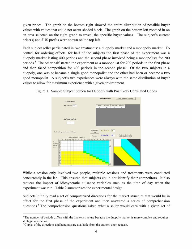
In our experiments, subject sellers post prices for truthfully revealing computerized buyers.2 A buyer visits the market every 3 seconds (called a period), observes the relevant price(s) and makes a purchase decision based upon the randomly determined values of VA and VB. Sellers receive feedback every period regarding their own profit and their rival’s price, if they are competing in a duopoly market. Our sellers can update their own prices at any time. As documented by Davis and Korenok (2009, p. 465), this approach “does indeed improve the drawing power of underlying equilibrium predictions.” As argued by Hampton and Sherstyuk (2010), to better replicate naturally occurring markets our duopoly sellers faced the same rival each period as is common in many market experiments. This design choice is expected to facilitate collusion (Dufwenberg and Gneezy 2002; Huck, et al. 2004), which should increase duopoly prices relative to those shown in the top row of Table 1.3 Having a fixed matching protocol also affords an opportunity to explore pricing dynamics as seller’s respond to each other.
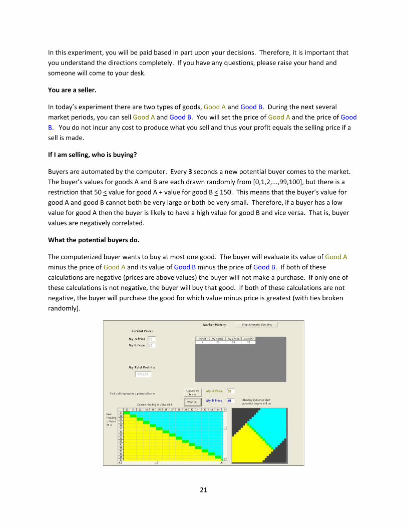
A sample screen shot is shown in Figure 1 for the duopoly market with positively correlated values. In addition to the feedback that subjects received every period (shown in the top right), they also had a “What if” tool that would identify the purchase decision of each buyer type for 2 Buyers demand at most one unit and, therefore, demand under-revelation is not an optimal buyer response.If buyers demand multiple units, then they may have market power which would enable them to under-reveal their demand, push prices down unilaterally generating more surplus for themselves. With a single unit of demand, under-revelation assures the buyer earns 0 and therefore the buyer would prefer to truthfully reveal demand by making a purchase at any price equal to or less than the buyer’s value. For a comparison of human and computer buyers in situations with market power, see Brown Kruse (2008). 3 While the set-up of C&R is a one shot game, pilot sessions conducted with subject sellers being randomly rematched with other sellers each period resulted in extremely low prices leading to the revised design.
given privalues wan area sprice(s) a
Each subcontrol fduopoly periods.4
and thenduopoly,good movalues to
F
While a concurrenreduces experime
Subjects effect foquestions
4 The numbstrategic in5 Copies of
ices. The gith values thselected on and $US pro
bject seller pfor ordering market lasti The other h
n faced com one was or
onopolist. Ao allow for m
Figure 1. Sa
session onlntly in the lthe impact
ent was run.
initially reaor the first s.5 The com
ber of periods nteraction. f the directions
graph on thehat could notthe right gr
ofits were sho
articipated ineffects, for
ing 400 perihalf started t
mpetition forr became a s
A subject’s twmaximum exp
ample Subje
ly involved ab. This enof idiosync Table 2 sum
ad a set of cophase of th
mprehension
differs with the
s and handouts
e bottom rigt occur shaderaph to reveown on the t
n two treatmr half of theods and the the experimer 400 periodsingle good mwo experiencperience wit
ct Screen fo
two peoplensured that scratic nuisanmmarizes the
omputerizedhe experimequestions a
e market struct
are available f
4
ght showed ted black. Thal the specitop left.
ments: a duope subjects thsecond pha
ent as a monds in the semonopolist ces were alwth a given en
r Duopoly w
, multiple ssubjects coulnce variablee experimen
d directions fent and thensked what a
ture because th
from the autho
the entire dhe graph on fic buyer va
poly markethe first phase involved nopolist for 2econd phaseand the otheways with thnvironment.
with Positive
sessions andld not identies such as
ntal design.
for the markn answered a seller wou
he duopoly mar
rs upon reques
distribution othe bottom lalues. The
and a monoase of the ex
being a mo200 periods . Of the twer had been he same dist
ely Correlate
d treatments ify their comthe time o
ket structure a series of
uld earn wit
rket is more co
st.
of possible bleft zoomed subject’s cu
opoly marketxperiment wnopolists foin the first p
wo subjectsor became a
tribution of b
ed Goods
were condumpetitors. Itof day when
that would f comprehenth a given s
omplex and req
buyer in on
urrent
t. To was a r 200 phase in a a two buyer
ucted t also n the
be in nsion set of
quires
5
prices for a series of possible buyer values. Once all subjects had completed the directions and had any questions answered privately, the first phase of the experiment began with each subject setting an initial price or prices. Once all of the subjects made this initial decision, buyers began visiting the market and making purchase decisions. The total number of periods in the market was unknown to the subjects. After the initial phase was completed, the second phase followed a similar process beginning with market structure specific computerized directions. After the second phase was completed, subjects were paid their earnings in private and dismissed from the experiment. Seller profits were converted to $US payments to the subjects at the rate 400 Profit = $1 US. The average salient payment was $24.20 for the approximately one hour experiment. Subjects also received a $7.00 participation payment.6
Table 2.Summary of Experiential Design
Condition Phase 1 Market
Structure
Phase 2 Market
Structure
Correlation of Values
Replications
1
Single Good Monopoly
Duopoly Positive 4 Two Good Monopoly
2
Single Good Monopoly
Duopoly Negative 4 Two Good Monopoly
3
Duopoly
Single Good Monopoly
Positive 4 Two Good Monopoly
4
Duopoly
Single Good Monopoly
Negative 4 Two Good Monopoly
Behavioral Results
We observed a total of 19,200 pricing decisions from 32 subject sellers (four replicates of each condition). These data are not independent, which we account for in subsequent statistical analysis. The results section is broken into two parts. In the first we consider the treatment effects. In the second we consider the dynamics of our duopoly markets.
6 This payment is standard at the Economic Science Institute at Chapman University where the experiments were conducted. The subjects were drawn from the undergraduate population at Chapman University. Some of the subjects had participated in other economics experiments, but none had previously been in any related experiments.
6
Treatment Effects
The average single good monopoly price across all observations was 43.54, which is nominally similar to the predicted price of 45. For duopolists, the average price was 29.03 when buyer values were positively correlated, not dissimilar to the predicted price of 32. When buyer values were negatively correlated, the average duopoly price was 31.39, similar to the positive correlation case and a change in the opposite direction from what was predicted.
This pattern seems to question the predictive success of C&R. However, this cursory comparison masks the result that single good monopoly prices differed dramatically based upon the correlation of buyer values even though this is theoretically irrelevant. The average single good monopoly price with positively correlated values 48.12, but the average single good monopoly price with negatively correlated value was only 38.96. A similar behavioral pattern is observed for two good monopolists as well. The average price set in the two good monopoly environment is 52.85 with positive correlation and only 48.25 with negative correlation even though the price is predicted to be 5 greater with negative correlation. Across all market structures, prices are systematically lower when buyer values are negatively correlated. Similarly, for both types of buyer values the change from a single good monopoly to a duopoly leads to price falling too much.7 In the case of positively correlated goods, the price reduction is 50% larger than predicted.
An overreaction to competition and a general price reduction due to goods being negatively correlated make observing the anticipated price increasing effect of competition unlikely. Still, one of our positively correlated buyer markets did see a higher average price under duopoly (PA = 39.44) than under a single good monopolist (PA = 36.63). The two identified behavioral patterns demonstrate the strength of laboratory research. By systematically controlling the variables of interest, one can identify treatment effects while controlling for commonalties across treatments. We do this by relying upon a linear mixed effects model where treatment effects are fixed but each subject has a random effect. This statistical approach allows us to fully exploit our data and controls for the repeated measures in the observations. Specifically we estimate the following model.
Pit= + 1Duopolyi+ 22Monopolyi+ 1Negativei
+1Negativei×Duopolyi+Negativei×2Monopolyi+ i + it (1)
Pit denotes the price set by subject i in period t.8 Duopoly and 2Monopoly are dummy variables
for the market structure and Negative is a dummy variable for the correlation of buyer values. i
is a subject specific random effect i.i.d. (0, 2) and it is an decision error term i.i.d (0,
2).
7 This result also suggests that the fixed matching protocol did not facilitate collusion as duopoly prices are dramatically lower than those set by two good monopolists regardless of the distribution of buyer values. 8 For a subject i in the role of a two good monopolist,Pit denotes the average of PA and PB in period t.
7
Before presenting our analysis of the estimation of the equilibrium price level, we recall that each subject seller participates in two treatments: an oligopoly market and a monopoly market. We separately estimated the following regression for each of the three treatments to analyze
whether any order effect exists or not: Pit= + 1Dummy_orderi+ i + eit. In this specification, Pit is the period t average price in duopoly market i, price set by single good monopolist i, or the average price set two good monopolist i, depending on treatment. Dummy_order is a dummy variable for the treatment occurring during phase 1 of the experiment. whether or not the
condition was . i is an individual specific random effect, i.i.d. (0, 2). The t-statistics for
Dummy_order are -0.142, -0.733 and -0.531 for the duopoly, single good monopoly, and two good monopoly treatments, respectively. None of these coefficients are significant and we conclude that there was no order effect and combine all of the data from a given treatment in our subsequent analysis. This result implies that there is no lasting effect on a monopolist from having experienced competition nor is there a lasting effect on competitive firms from having been monopolists regardless of the distribution of buyer values. The implication is that it is reasonable for policy makers to focus on the post proscription market structure without worrying about the history that led up to that point.
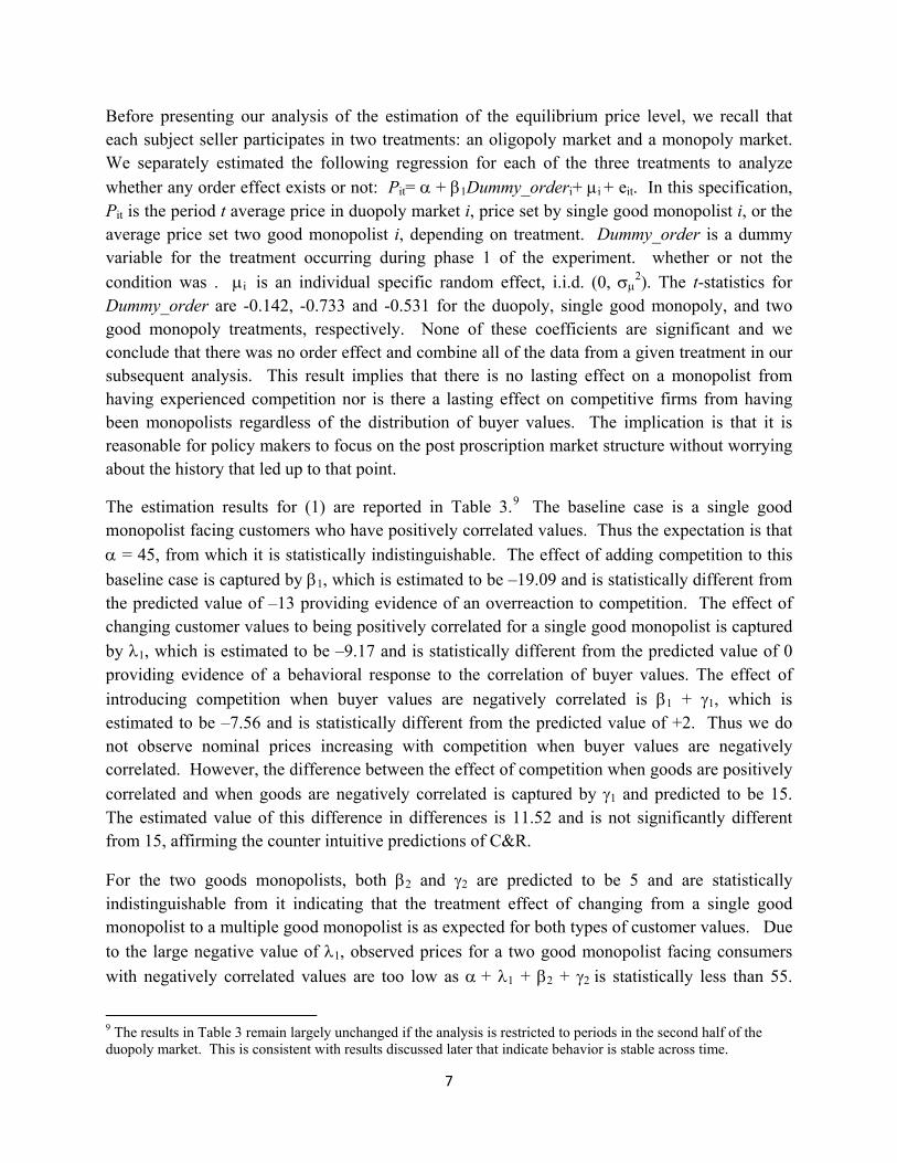
The estimation results for (1) are reported in Table 3.9 The baseline case is a single good monopolist facing customers who have positively correlated values. Thus the expectation is that
= 45, from which it is statistically indistinguishable. The effect of adding competition to this
baseline case is captured by 1, which is estimated to be –19.09 and is statistically different from the predicted value of –13 providing evidence of an overreaction to competition. The effect of changing customer values to being positively correlated for a single good monopolist is captured
by 1, which is estimated to be –9.17 and is statistically different from the predicted value of 0 providing evidence of a behavioral response to the correlation of buyer values. The effect of
introducing competition when buyer values are negatively correlated is 1 + 1, which is estimated to be –7.56 and is statistically different from the predicted value of +2. Thus we do not observe nominal prices increasing with competition when buyer values are negatively correlated. However, the difference between the effect of competition when goods are positively
correlated and when goods are negatively correlated is captured by 1 and predicted to be 15. The estimated value of this difference in differences is 11.52 and is not significantly different from 15, affirming the counter intuitive predictions of C&R.
For the two goods monopolists, both 2 and 2 are predicted to be 5 and are statistically indistinguishable from it indicating that the treatment effect of changing from a single good monopolist to a multiple good monopolist is as expected for both types of customer values. Due
to the large negative value of 1, observed prices for a two good monopolist facing consumers
with negatively correlated values are too low as + 1 + 2 + 2 is statistically less than 55.
9 The results in Table 3 remain largely unchanged if the analysis is restricted to periods in the second half of the duopoly market. This is consistent with results discussed later that indicate behavior is stable across time.
8
Observed prices for two good monopolists facing customers with positively correlated values are
as predicted, i.e. + 2 = 50.
Table 3. Statistical Analysis Based Upon Linear Mixed Effects Model
Estimation of Pi,t= + 1Duopolyi+ 22Monopolyi+ 1Negativei+1Negativei×Duopolyi+Negativei×2Monopolyi+ i + i,t
Parameter Coefficient Estimate Standard Error Ho: p-value
Constant 48.12 3.09 = 45 0.312 1 Duopoly –19.09 4.73 1= –13 <0.001 2 2Monopoly 4.73 4.37 2 = 5 0.950 1 Negative –9.17 4.37 1= 0 0.036 1 Negative×Duopoly 11.53 6.17 1 = 15 0.574 Negative×2Monopoly 4.56 6.18 = 5 0.944
Price Predictions Buyer Values Market Structure Ho: Estimate p-value
Positive Single Good Monopoly 48.12 0.312 Positive Two Good Monopoly + 2 = 50 52.85 0.357 Positive Duopoly + 1 = 32 29.03 0.336 Negative Single Good Monopoly + 1 = 45 38.95 0.050 Negative Two Good Monopoly + 1 + 2 + = 55 48.25 <0.001 Negative Duopoly + 1 + 1 + = 47 31.39 0.000
Treatment Effects
Buyer Values Treatment Effect Ho: Estimate p-value Positive Single Good Monopoly
Duopoly 1= –13 –19.09 <0.001
Negative 1 + = 2 0.029 Positive Single Good Monopoly
Two Good Monopoly 2 = 5 4.73 0.950
Negative 2 + = 10
0.871
Dynamics in the Duopoly Markets
Our data set also allows us to examine the dynamic interaction of the duopolists and see if this interaction differs with the distribution of values.10 In the case of negatively correlated values, the market share effect associated with a price change is small as compared to the positive
10 This analysis is also important because, while the model of Chen and Riordan (2008) is a one shot game, many naturally occurring markets are better described as repeated play games.
9
correlation case because fewer customers are indifferent between the two sellers at any given price pair. Therefore, we would expect that dupolists are more sensitive to their rivals when buyer values are positively correlated.
First, we ask whether or not subjects are in fact reacting to each other. For this we rely upon both a Granger (1969) causality test of lagged rival price controlling for own lagged price and the construction of a VAR model of prices. For the Granger causality test, we consider whether adding the lagged value of one’s rival’s price improves the estimation of an autoregressive model of one’s own duopoly price. The reduced-form bivariate vector autoregressive (VAR) model lag polynomials of order p is
t
p
jjtj
p
iitit uyxy ,1
1,1
1,10,1
(2)
t
p
jjtj
p
iitit uyxx ,2
1,2
1,20,2
(3)
where yt and xt denote period t prices by the two sellers, ),0.(..~ 2, iti diiu for i = 1, 2 and the
length p is determined by Akaike Information Criterion (AIC) or Schwarz Criterion (SIC). If the coefficients pii ,...,1,2,,1 in equation (2) are jointly significant different from zero, the null
hypothesis that x does not Granger causes y will be rejected. Similarly, if the coefficients
pjj ,...,2,1,,2 in equation (3) are jointly significant different from zero, the null hypothesis
y does not Granger causes x will be rejected.
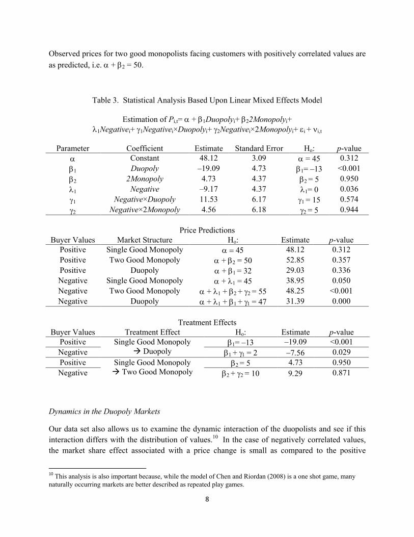
These results are important for parallelism between the lab and the field. If our sellers were not reacting to each other, then it would be unclear how valid our comparative results would be outside the lab assuming naturally occurring duopolists do react to their rivals. However, this is not the case here as our subject sellers are quickly responding to each other. Table 4 provides the statistical analysis. The first two columns in Table 4 give the p-value of the Granger Causality test for the positively related values. The last two columns give the results of negatively related values. Markets 1 to 4 are the sessions where the subjects experienced duopoly first. Markets 5 to 8 are the sessions where the subjects are initially monopolists.11
For all 16 pairs of subjects, we observe that market prices are reacting to previous prices. In half of the positively correlated buyer value sessions both sellers are reacting to their rival. The other half can be described as cases where there is a market leader who does not respond to his rival,
11 The market number is for expositional purposes. As discussed in the experiential design section, multiple sessions and treatments were conducted concurrently. It was not the case that all duopoly first experiments were conducted prior to the monopoly first experiments. The designation of PA and PB is arbitrary and done for exposition. All subjects had information presented to them as though he or she sold good A and that one’s rival sold good B. All single good monopolists sold good A.
10
but is responded to by his rival. For the markets with negatively correlated values, there were three instances in which both sellers strongly Granger caused each other to adjust prices and the five remaining markets had a market leader. There is no apparent difference between markets with positively and negatively correlated buyer values nor is there anything to suggest an order effect.
Table 4. p-values Associated with Test that Rival’s Price GrangerCauses Own Price
Positive Correlation Negative Correlation Ho: PAdoes not
Granger Causes PB Ho: PB does not
Granger Causes PA
Ho: PA does not Granger Causes PB
Ho: PB does not Granger Causes PA
Market 1 <0.001 <0.001 0.201 0.067 Market 2 <0.001 0.056 <0.001 0.036 Market 3 0.791 0.001 <0.001 0.005 Market 4 <0.001 0.951 0.005 0.522 Market 5 0.001 0.605 0.750 <0.001 Market 6 0.164 0.017 <0.001 0.193 Market 7 <0.001 0.093 0.003 0.809 Market 8 0.010 <0.001 0.007 0.029
Next we turn to a VAR model of pricing dynamics. We check each duopoly market’s price path for a unit root based on augmented Dickey-Fuller (ADF) test. For 31 of the 32 sellers we can strongly reject the existence of a unit root implying that these sellers have stationary prices that we can investigate using a VAR model based on the price levels. Optimal lag length is determined jointly for the two sellers in a market using the Bayesian Information Criteria (BIC). For 12 marketsthe best lag length is 1, a three second delay in responding. For three of the markets the best lag length is 2 and for the remaining market it is 4.12 Of the markets with negatively correlated values, only one market had a lag length greater than 1 and it had a lag of 2.
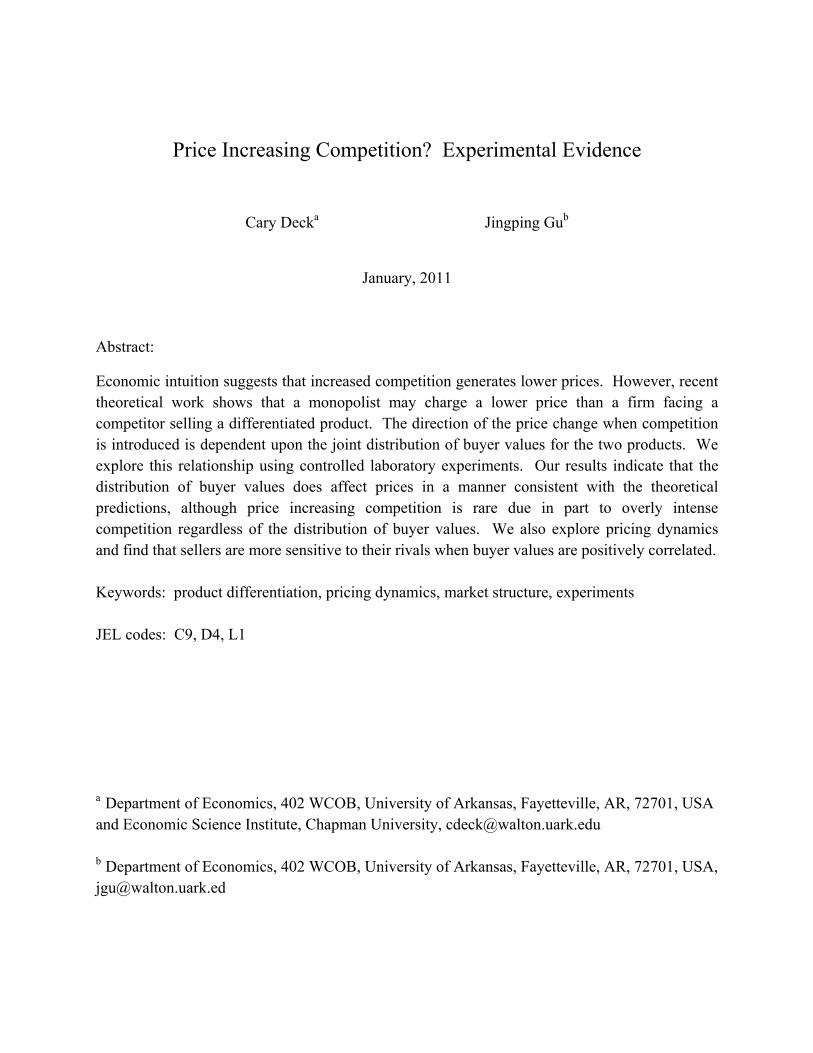
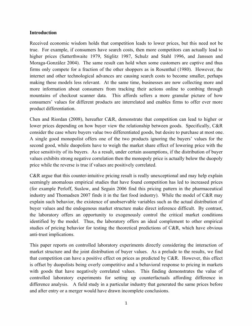
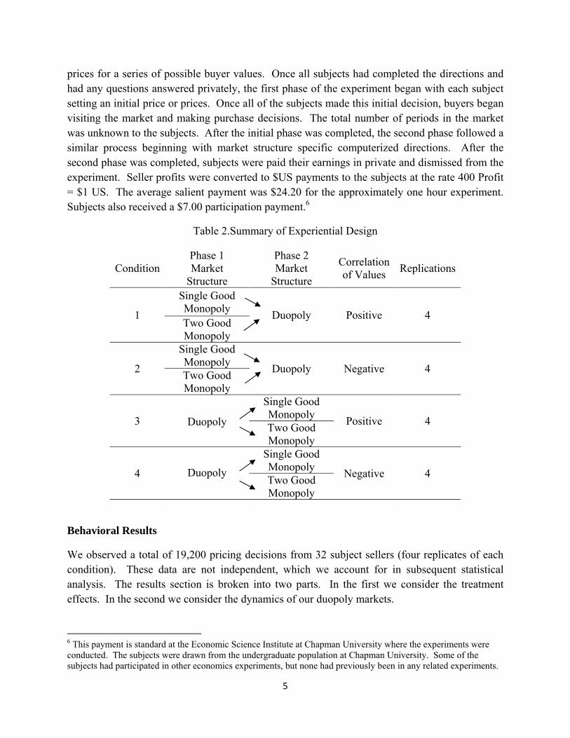
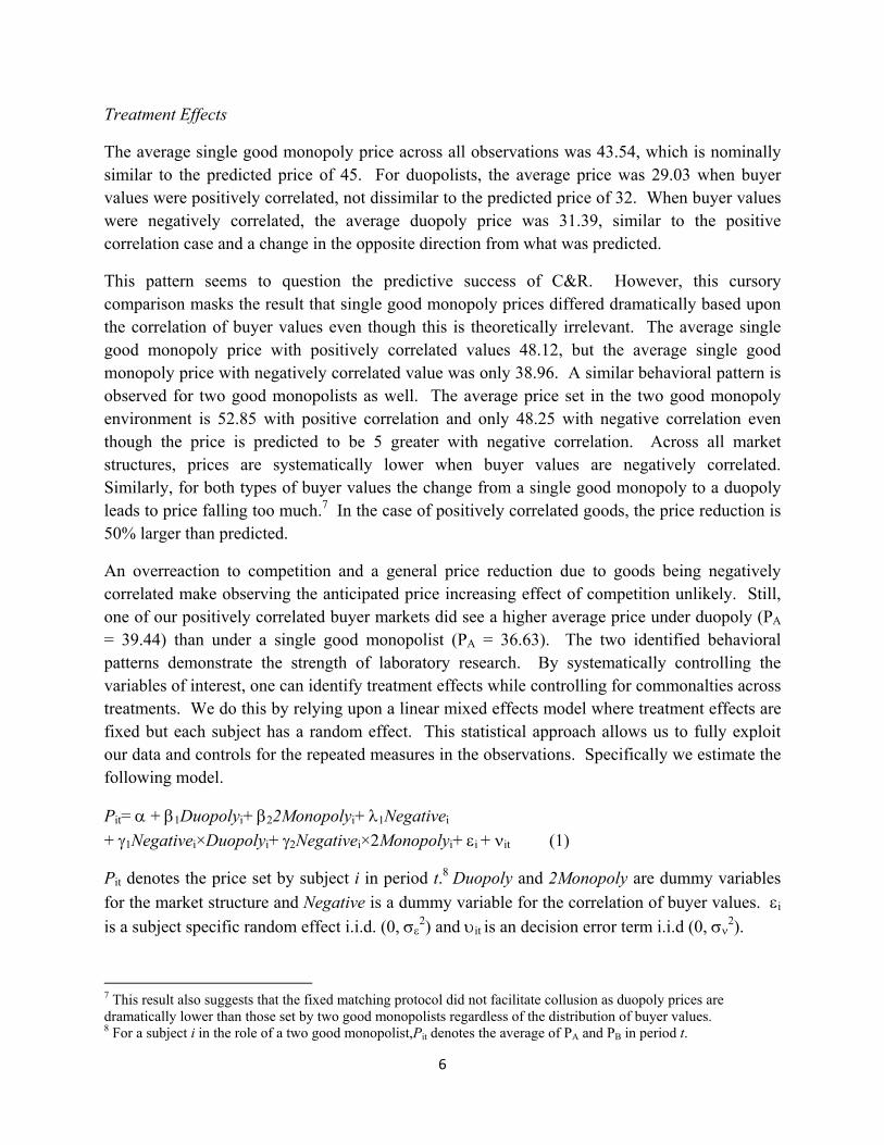
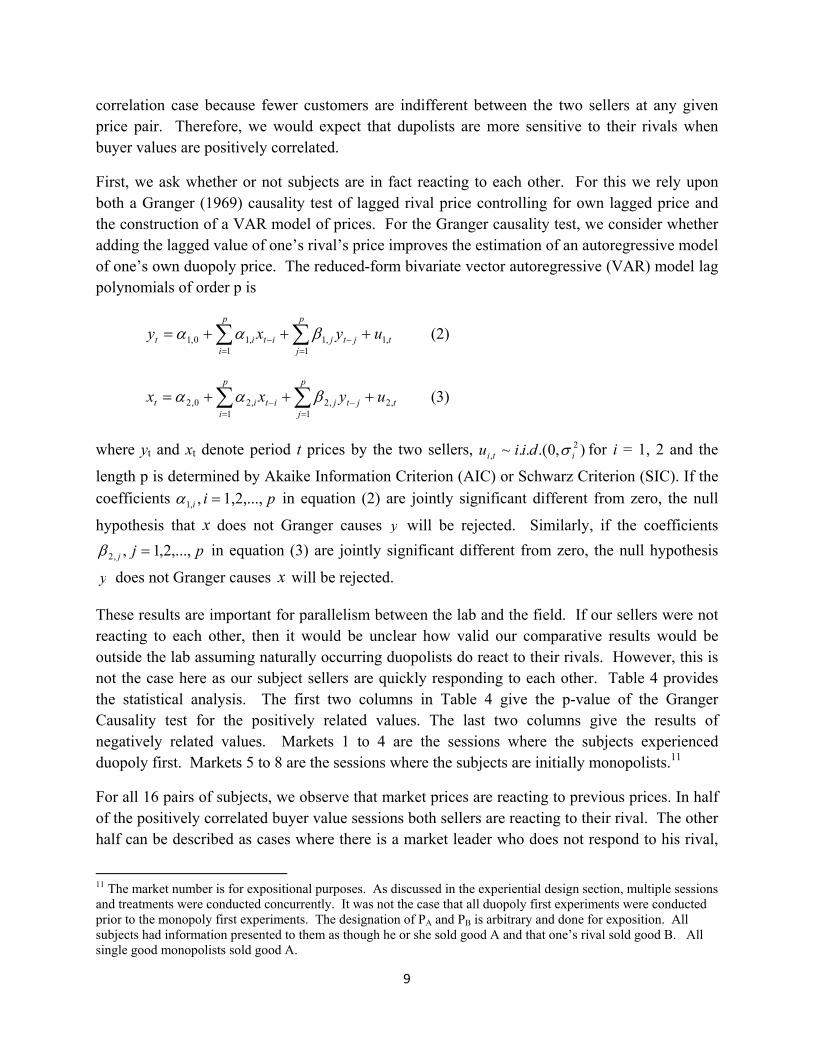
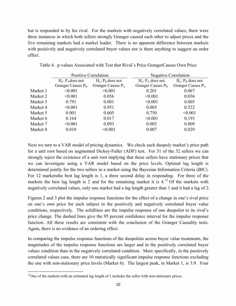
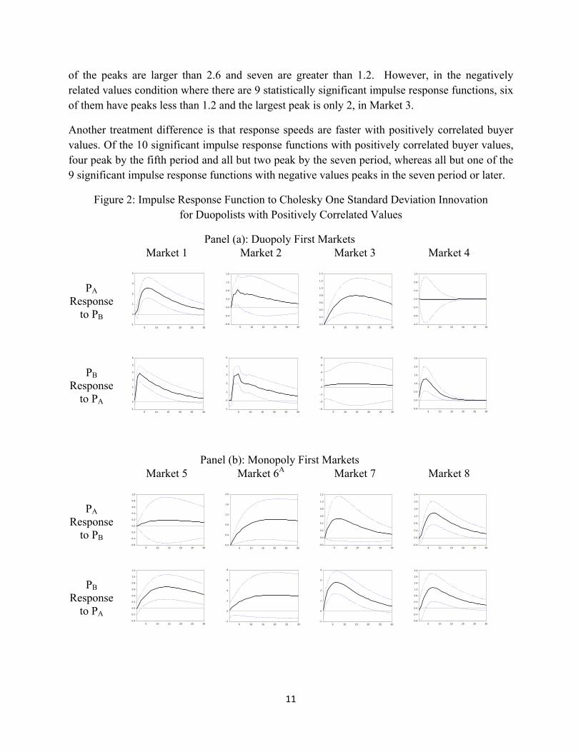
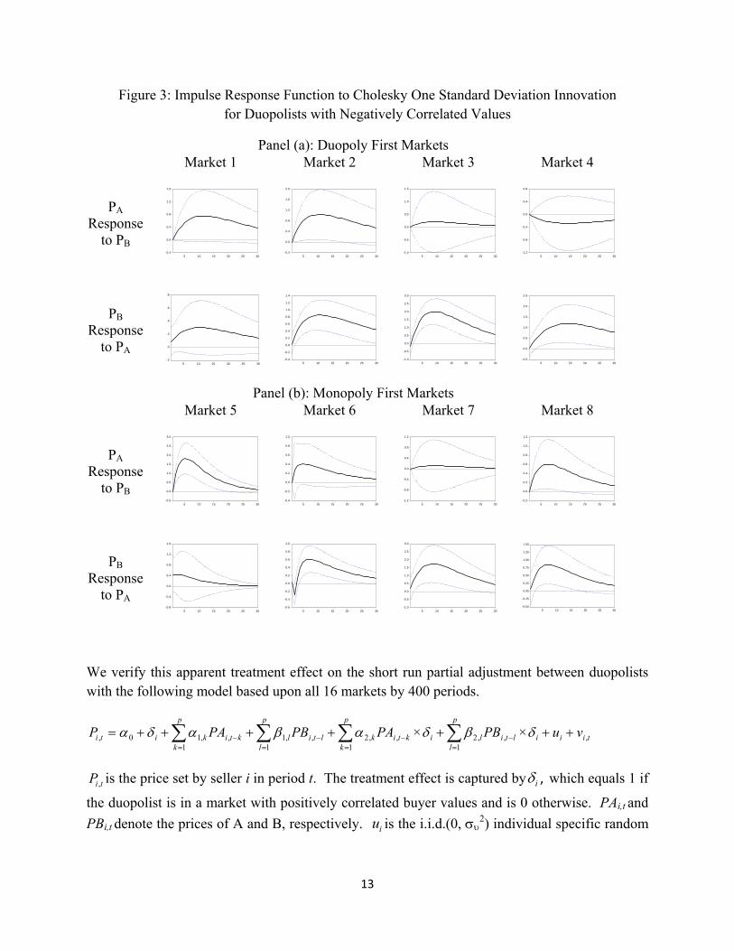
Figures 2 and 3 plot the impulse response functions for the effect of a change in one’s rival price on one’s own price for each subject in the positively and negatively correlated buyer value conditions, respectively. The solidlines are the impulse response of one duopolist to its rival’s price change. The dashed lines give the 95 percent confidence interval for the impulse response function. All these results are consistent with the conclusion of the Granger Causality tests. Again, there is no evidence of an ordering effect.
In comparing the impulse response functions of the duopolists across buyer value treatments, the magnitudes of the impulse response functions are larger and in the positively correlated buyer values condition than in the negatively correlated condition. More specifically, in the positively correlated values case, there are 10 statistically significant impulse response functions excluding the one with non-stationary price levels (Market 6). The largest peak, in Market 1, is 3.9. Four
12One of the markets with an estimated lag length of 1 includes the seller with non-stationary prices.
11
of the peaks are larger than 2.6 and seven are greater than 1.2. However, in the negatively related values condition where there are 9 statistically significant impulse response functions, six of them have peaks less than 1.2 and the largest peak is only 2, in Market 3.
Another treatment difference is that response speeds are faster with positively correlated buyer values. Of the 10 significant impulse response functions with positively correlated buyer values, four peak by the fifth period and all but two peak by the seven period, whereas all but one of the 9 significant impulse response functions with negative values peaks in the seven period or later.
Figure 2: Impulse Response Function to Cholesky One Standard Deviation Innovation for Duopolists with Positively Correlated Values
Panel (a): Duopoly First Markets Market 1 Market 2 Market 3 Market 4
PA Response
to PB
PB Response
to PA
Panel (b): Monopoly First Markets Market 5 Market 6A Market 7 Market 8
PA Response
to PB
PB Response
to PA
-1
0
1
2
3
4
5 10 15 20 25 30
-0.8
-0.4
0.0
0.4
0.8
1.2
1.6
5 10 15 20 25 300.0
0.2
0.4
0.6
0.8
1.0
1.2
1.4
5 10 15 20 25 30-1.2
-0.8
-0.4
0.0
0.4
0.8
1.2
5 10 15 20 25 30
-1
0
1
2
3
4
5
6
5 10 15 20 25 30-1
0
1
2
3
4
5
5 10 15 20 25 30-.6
-.4
-.2
.0
.2
.4
.6
.8
5 10 15 20 25 30
-0.5
0.0
0.5
1.0
1.5
2.0
2.5
5 10 15 20 25 30
-0.6
-0.4
-0.2
0.0
0.2
0.4
0.6
0.8
1.0
5 10 15 20 25 300.0
0.4
0.8
1.2
1.6
2.0
5 10 15 20 25 30-0.2
0.0
0.2
0.4
0.6
0.8
1.0
1.2
5 10 15 20 25 30-0.4
0.0
0.4
0.8
1.2
1.6
2.0
2.4
5 10 15 20 25 30
-0.4
-0.2
0.0
0.2
0.4
0.6
0.8
1.0
1.2
5 10 15 20 25 30-.2
.0
.2
.4
.6
.8
5 10 15 20 25 30-1
0
1
2
3
4
5 10 15 20 25 30
-0.8
-0.4
0.0
0.4
0.8
1.2
1.6
2.0
2.4
5 10 15 20 25 30

12
A In this market, one of two sellers prices is nonstationary.
13
Figure 3: Impulse Response Function to Cholesky One Standard Deviation Innovation for Duopolists with Negatively Correlated Values
Panel (a): Duopoly First Markets Market 1 Market 2 Market 3 Market 4
PA Response
to PB
PB Response
to PA
Panel (b): Monopoly First Markets Market 5 Market 6 Market 7 Market 8
PA Response
to PB
PB Response
to PA
We verify this apparent treatment effect on the short run partial adjustment between duopolists with the following model based upon all 16 markets by 400 periods.
tiii
p
lltil
p
kiktik
p
lltil
p
kktikiti vuPBPAPBPAP ,
1,,2
1,,2
1,,1
1,,10, ××
tiP, is the price set by seller i in period t. The treatment effect is captured by i , which equals 1 if
the duopolist is in a market with positively correlated buyer values and is 0 otherwise. PAi,t and
PBi,t denote the prices of A and B, respectively. iu is the i.i.d.(0, 2) individual specific random
-0.4
0.0
0.4
0.8
1.2
1.6
5 10 15 20 25 30-0.4
0.0
0.4
0.8
1.2
1.6
2.0
5 10 15 20 25 30-1.0
-0.5
0.0
0.5
1.0
1.5
5 10 15 20 25 30-1.2
-0.8
-0.4
0.0
0.4
0.8
5 10 15 20 25 30
-.2
.0
.2
.4
.6
.8
5 10 15 20 25 30
-0.4
-0.2
0.0
0.2
0.4
0.6
0.8
1.0
1.2
1.4
5 10 15 20 25 30-1.0
-0.5
0.0
0.5
1.0
1.5
2.0
2.5
3.0
5 10 15 20 25 30-0.5
0.0
0.5
1.0
1.5
2.0
2.5
5 10 15 20 25 30
-0.5
0.0
0.5
1.0
1.5
2.0
2.5
3.0
5 10 15 20 25 30-0.4
-0.2
0.0
0.2
0.4
0.6
0.8
1.0
5 10 15 20 25 30-1.2
-0.8
-0.4
0.0
0.4
0.8
1.2
5 10 15 20 25 30-0.2
0.0
0.2
0.4
0.6
0.8
1.0
1.2
5 10 15 20 25 30
-0.8
-0.4
0.0
0.4
0.8
1.2
1.6
5 10 15 20 25 30-0.6
-0.4
-0.2
0.0
0.2
0.4
0.6
0.8
1.0
5 10 15 20 25 30-1.0
-0.5
0.0
0.5
1.0
1.5
2.0
2.5
3.0
5 10 15 20 25 30
-0.50
-0.25
0.00
0.25
0.50
0.75
1.00
1.25
1.50
5 10 15 20 25 30
14
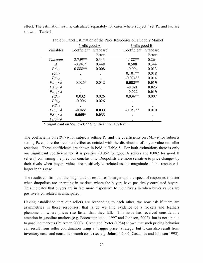
effect. The estimation results, calculated separately for cases where subject i set PA and PB, are shown in Table 5.
Table 5: Panel Estimation of the Price Responses on Duopoly Market i sells good A i sells good B
Variables Coefficient Standard Error
Coefficient Standard Error
Constant 2.759** 0.343 1.188** 0.264 Δ -0.943* 0.448 0.508 0.344
PAt-1 0.888** 0.008 -0.004 0.013 PAt-2 . . 0.101** 0.018 PAt-3 . . -0.074** 0.014
PAt-1×δ -0.026* 0.012 0.082** 0.019 PAt-2×δ . . -0.021 0.025 PAt-3×δ . . -0.022 0.019
PBt-1 0.032 0.026 0.936** 0.007 PBt-2 -0.006 0.026 . . PBt-3 . . .
PBt-1×δ -0.022 0.033 -0.057** 0.010 PBt-2×δ 0.069* 0.033 . . PBt-3×δ . . .
* Significant on 5% level;** Significant on 1% level.
The coefficients on PBt-i×δ for subjects setting PA and the coefficients on PAt-i×δ for subjects setting PB capture the treatment effect associated with the distribution of buyer valueson seller reactions. These coefficients are shown in bold in Table 5. For both estimations there is only one significant coefficient and it is positive (0.069 for good A sellers and 0.082 for good B sellers), confirming the previous conclusions. Duopolists are more sensitive to price changes by their rivals when buyers values are positively correlated as the magnitude of the response is larger in this case.
The results confirm that the magnitude of responses is larger and the speed of responses is faster when duopolists are operating in markets where the buyers have positively correlated buyers. This indicates that buyers are in fact more responsive to their rivals in when buyer values are positively correlated as anticipated.
Having established that our sellers are responding to each other, we now ask if there are asymmetries in those responses; that is do we find evidence of a rockets and feathers phenomenon where prices rise faster than they fall. This issue has received considerable attention in gasoline markets (e.g. Borenstein et al., 1997 and Johnson, 2002), but is not unique to gasoline markets (Peltzman 2000). Green and Porter (1984) shown that such pricing behavior can result from seller coordination using a “trigger price” strategy, but it can also result from inventory costs and consumer search costs (see e.g. Johnson 2002, Castanias and Johnson 1993).
15
In experimental work, Deck and Wilson (2008) found evidence of rockets and feathers reactions to changes in input costs.13 Our data set allows us to investigate the downward stickiness of a generic market where sellers cannot communicate, all information is perfectly observable, and costs are held constant.
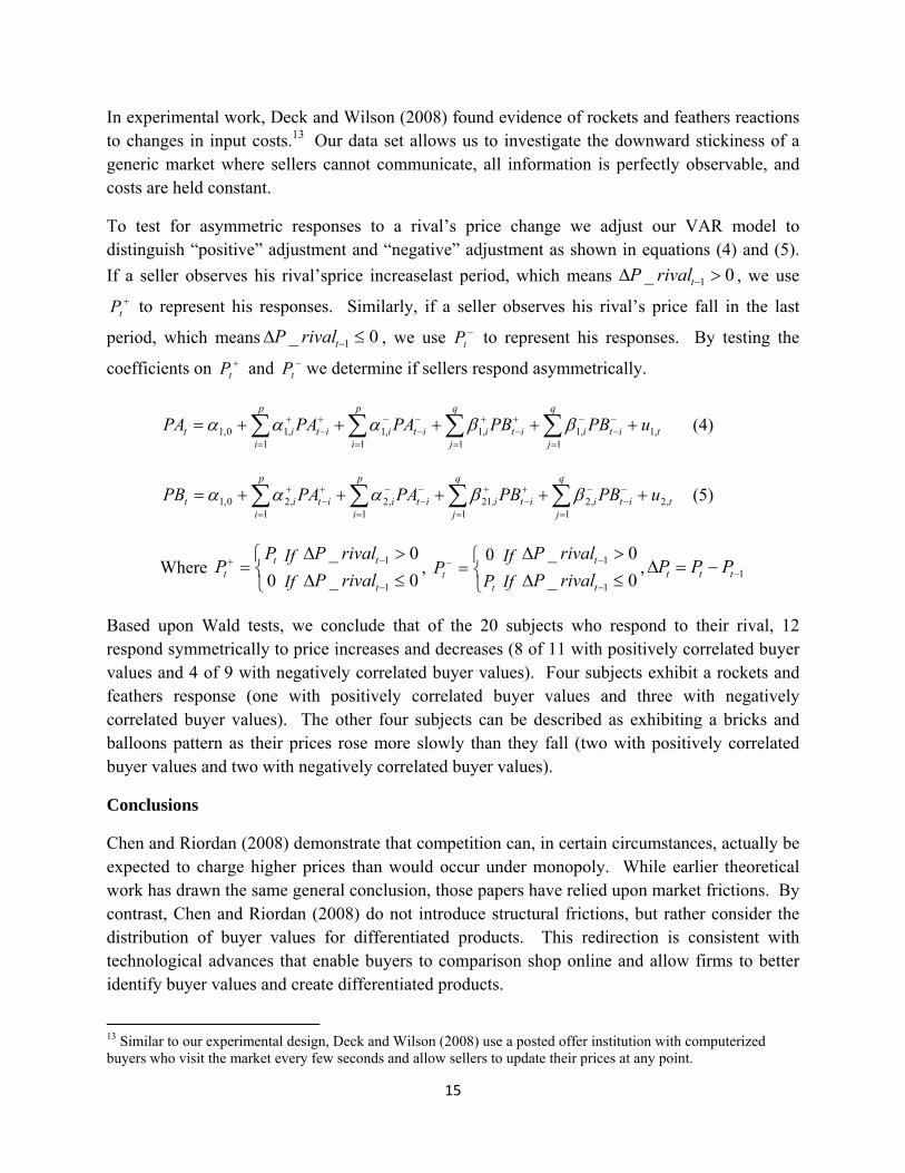
To test for asymmetric responses to a rival’s price change we adjust our VAR model to distinguish “positive” adjustment and “negative” adjustment as shown in equations (4) and (5).
If a seller observes his rival’sprice increaselast period, which means 0_ 1 trivalP , we use
tP to represent his responses. Similarly, if a seller observes his rival’s price fall in the last
period, which means 0_ 1 trivalP , we use tP to represent his responses. By testing the
coefficients on tP and
tP we determine if sellers respond asymmetrically.
t
q
jiti
q
jiti
p
iiti
p
iitit uPBPBPAPAPA ,1
1,1
1,1
1,1
1,10,1
(4)
t
q
jiti
q
jiti
p
iiti
p
iitit uPBPBPAPAPB ,2
1,2
1,21
1,2
1,20,1
(5)
Where
0t
t
PP
If
If
0_
0_
1
1
t
t
rivalP
rivalP,
tt P
P0
If
If
0_
0_
1
1
t
t
rivalP
rivalP, 1 ttt PPP
Based upon Wald tests, we conclude that of the 20 subjects who respond to their rival, 12 respond symmetrically to price increases and decreases (8 of 11 with positively correlated buyer values and 4 of 9 with negatively correlated buyer values). Four subjects exhibit a rockets and feathers response (one with positively correlated buyer values and three with negatively correlated buyer values). The other four subjects can be described as exhibiting a bricks and balloons pattern as their prices rose more slowly than they fall (two with positively correlated buyer values and two with negatively correlated buyer values).
Conclusions
Chen and Riordan (2008) demonstrate that competition can, in certain circumstances, actually be expected to charge higher prices than would occur under monopoly. While earlier theoretical work has drawn the same general conclusion, those papers have relied upon market frictions. By contrast, Chen and Riordan (2008) do not introduce structural frictions, but rather consider the distribution of buyer values for differentiated products. This redirection is consistent with technological advances that enable buyers to comparison shop online and allow firms to better identify buyer values and create differentiated products.
13 Similar to our experimental design, Deck and Wilson (2008) use a posted offer institution with computerized buyers who visit the market every few seconds and allow sellers to update their prices at any point.

16
Before relying upon any model to make inference, one must subject the model to testing. At current, some empirical evidence is consistent with the results of Chen and Riordan (2008); however, it can be difficult to determine if any particular naturally occurring market fits the necessary assumptions identified in the theoretical model. Therefore, this paper uses controlled experiments to test Chen and Riordan (2008). The laboratory offers a means to exogenously manipulate the model’s identified factors and test its predictions.
Our experimental findings indicate the effect of competition does depend on the degree of correlation in buyer values, consistent with the theoretical predictions. However, we also observe two unexpected behavioral patterns. First, subject sellers of differentiated products overreact to competition in both of our buyer value environments. Second, prices are low when buyer values are negatively correlated, regardless of the market structure we implement. These two findings work against the nominal price increase predicted by Chen and Riordan (2008) and in fact we would have wrongly concluded that their model’s predictions did not hold if we had only observed markets with negative correlation or had only focused on duopoly markets.
Our within subject experimental design also enables us to look for possible hysteresis effects on market structure. Should such effects exist, one would need to be concerned with the path that led to a particular market structure when predicting behavior in a given market. However, we find no evidence of such effects, suggesting that a two good monopolist forced to spin off one product line will behave the same as a former single good monopolist facing a new entrant and competitors that have never been in a monopoly situation.
In terms of pricing dynamics in our duopoly markets, we find that prices are generally stable over time regardless of buyer values. However, differentiated product duopolists are more sensitive to their rival’s behavior when buyer values are positively correlated, as expected, since the market share effect of a price change is relatively large in this case. This greater sensitivity is manifest both in the size and speed of the response function. In a few of our markets we observe prices increasing faster than they fall, a rockets and feathers result, but price reactions are more frequently symmetric.
17
References
Aloysius, J., Deck, C., and Farmer, A. 2010. "A Comparison of Bundling and Sequential Pricing in Competitive Markets: Experiential Evidence" International Journal of the Economics of Business, forthcoming
Borenstein, S., Cameron, A., and Gilbert, R. 1997.“Do Gasoline Prices Respond Asymmetrically to Crude Oil Price Changes?”Quarterly Journal of Economics 112, pp. 305-39.
Brown Kruse, J. 2008. “Simulated and Real Buyers in Posted Offer Markets.”Handbook of Experimental Results, Vol. 1, Vernon L. Smith and Charles Plott, eds, North Holland/Elsevier Press, Amsterdam, pp. 71-76.
Castanias, R.and Johnson, H. 1993. “Gas Wars: Retail Gasoline Fluctuations.”Review of Economics and Statistics 75, pp. 171-74
Chen, Y., and Riordan M. 2008.“Price-increasing Competition.”Rand Journal of Economics,
39(4), pp. 1042-58. Davis, D. and Holt, C. 1993. Experimental Economics.Princeton University Press: Princeton
N.J. Davis, D. and Korenok, O. 2009. “Posted-Offer Markets in Near Continuous Time: An
Experimental Investigation.”Economic Inquiry ,47, pp. 446-466 Deck, C. and B. Wilson. 2008. “Experimental Gasoline Markets.” Journal of Economic Behavior
and Organization 67(1), pp. 134-149. Dufwenberg, M. and Gneezy, U. 2000. “Price Competition and Market Concentration: An
Experimental Study.” International Journal of Industrial Organization 18(1), pp. 7-22. Green, E., and Porter, R. 1984. “Non-cooperative Collusion under Imperfect Price Information.”
Econometrica, 52(1), pp. 87-100. Hampton, K. and Sherstyuk, K. 2010. “Demand Shocks, Capacity Coordination and Industry
Performance: Lessons from Economic Laboratory.” Working Paper, University of Hawaii.
Huck, S., Normann, H., and Oechssler, J. 2004. “Two Are Few and Four Are Many: Number
Effects in Experimental Oligopolies.” Journal of Economic Behavior and Organization 53(4), pp. 435-446.
18
Janssen, M., and Moraga-González, J. 2004. "Strategic Pricing, Consumer Search and
the Number of Firms" Review of Economic Studies 71, pp. 1089-1118. Johnson, R. 2002. “Search Costs, Lags, and Prices at the Pump.”Review of Industrial
Organization 20, pp. 33-50. Perloff, J., Suslow, V., and Seguin, P.2006. “Higher Prices from Entry: Pricing of Brand-Name
Drugs.” Mimeo, University of California–Berkeley. Peltzman, S. 2000. “Prices Rise Faster Than They Fall.”Journal of Political Economy 108, pp.
466-502. Rosenthal, R. 1980. “A Model in Which an Increase in the Number of Sellers Leads to a
Higher Price." Econometrica 48, pp. 1575-1579. Satterthwaite, M. 1979. “Consumer Information, Equilibrium Industry Price, and the
Number of Sellers." Bell Journal of Economics 10, pp. 483-502. Schulz, N., and Stahl. K. 1996. “Do Consumers Search for the Higher Price? Oligopoly
Equilibrium and Monopoly Optimum in Differentiated-Products Markets." Rand Journal of Economics 27, pp. 542-562.
Stiglitz, J. 1987. “Competition and the Number of Firms in a Market: Are Duopolists
More Competitive Than Atomistic Markets?" Journal of Political Economy 95, pp. 1041- 1061.
Thomadsen, R. 2007. “Product Positioning and Competition: The Role of Location in the Fast Food Industry.”Marketing Science, 26, pp. 792–804.

Appendi
In this exp
you unde
someone
You are a
In today’s
market pe
do not inc
made.
If I am sel
Buyers ar
The buyer
restriction
good A an
value for g
values are
What the
The comp
minus the
purchase.
ix: Directio
periment, you
rstand the dir
will come to
seller.
s experiment
eriods, you ca
cur any cost t
lling, who is b
e automated
r’s values for
n that 50 < va
nd good B can
good A then t
e negatively c
potential bu
puterized buy
e price of Goo
. If this calcu
ons and Han
u will be paid
rections com
your desk.
there are two
an sell Good A
o produce wh
buying?
by the comp
goods A and
alue for good
nnot both be
the buyer is l
correlated.
uyers do.
yer wants to b
od A. If this c
lation is not n
ndout for Du
based in part
pletely. If yo
o types of goo
A but no one
hat you sell a
puter. Every 3
B are each dr
A + value for
very large or
ikely to have
buy at most o
alculation is n
negative, the
19
uopoly with
t upon your d
u have any q
ods, Good A a
is selling Goo
nd thus your
3 seconds a n
rawn random
r good B < 150
both be very
a high value
ne good. The
negative (pric
buyer will pu
h Negatively
decisions. Th
uestions, plea
and Good B.
od B. You wil
profit equals
ew potential
mly from [0,1,
0. This mean
y small. There
for good B an
e buyer will e
ce is above va
urchase Good
y Correlated
erefore, it is
ase raise you
During the n
l set the price
s the selling p
buyer comes
2,...,99,100],
s that the bu
efore, if a buy
nd vice versa.
evaluate its va
alue) the buye
d A.
d Values
important th
r hand and
ext several
e of Good A.
price if a sell is
s to the mark
but there is a
yer’s value fo
yer has a low
. That is, buy
alue of Good
er will not ma
at
You
s
et.
a
or
yer
A
ake a

20
“What if” Pricing Tool
The bottom half of your screen (which is shown on the previous page) provides a tool that allows you to
see what would happen for different prices. For whatever price you provide, you can press the “What
if...” button and the table in the lower right will shade yellow the region of buyers who will buy good A.
The region that is white represents buyers who would not buy anything given the prices. Buyer values
cannot be drawn from the region that is shaded black.
The table on the left is also color‐coded. Clicking on a cell in the right table will cause the left table to
zoom in on that area. The two tables present the same information; the right table is zoomed out so
you can see all potential buyers and the left table is zoomed in so you can see the specific values of each
potential buyer that could be randomly selected.
Changing my Price
You will set your initial price in the upper left hand portion of your screen by entering your price and
pressing “Set my Price”. During the experiment you can update your price by typing the price you want
to charge on the bottom left portion of your screen (by the “What if tool”) and pressing “Update my
Price.”
Feedback During Market Session
The top right of your screen gives you all of the information from the market under the heading “Market
History.” You can observe what price was charged and what if any profit you earned. This information
is updated every 3 seconds as a new potential buyer enters the market. The default setting is that the
table will automatically scroll down as new information appears, but you can stop scrolling by pressing
the “Stop Automatic Scrolling” button and restart it by pressing the button again.
The top left of your screen also shows your current total payoff, which you will be paid at the end of the
experiment. Your firm’s profit are converted into $US at the rate of 400 in profit = $1.
Your current price is also displayed in the top left portion of your screen as well.
If you have any questions, please raise your hand. Remember that you are paid based upon your
decisions so it is important that you understand the directions completely. If you do not have any
questions, please press the green button labeled “I am done with the directions.”
In this exp
you unde
someone
You are a
In today’s
market pe
B. You do
sell is mad
If I am sel
Buyers ar
The buyer
restriction
good A an
value for g
values are
What the
The comp
minus the
calculatio
these calc
negative,
randomly
periment, you
rstand the dir
will come to
seller.
s experiment
eriods, you ca
o not incur an
de.
lling, who is b
e automated
r’s values for
n that 50 < va
nd good B can
good A then t
e negatively c
potential bu
puterized buy
e price of Goo
ns are negati
culations is no
the buyer wi
y).
u will be paid
rections com
your desk.
there are two
an sell Good A
ny cost to pro
buying?
by the comp
goods A and
alue for good
nnot both be
the buyer is l
correlated.
uyers do.
yer wants to b
od A and its v
ve (prices are
ot negative, t
ll purchase th
based in part
pletely. If yo
o types of goo
A and Good B
oduce what yo
puter. Every 3
B are each dr
A + value for
very large or
ikely to have
buy at most o
alue of Good
e above value
he buyer will
he good for w
21
t upon your d
u have any q
ods, Good A a
B. You will set
ou sell and th
3 seconds a n
rawn random
r good B < 150
both be very
a high value
ne good. The
B minus the
es) the buyer
buy that goo
which value m
decisions. Th
uestions, plea
and Good B.
t the price of
hus your prof
ew potential
mly from [0,1,
0. This mean
y small. There
for good B an
e buyer will e
price of Good
will not make
od. If both of
minus price is g
erefore, it is
ase raise you
During the n
f Good A and
fit equals the
buyer comes
2,...,99,100],
s that the bu
efore, if a buy
nd vice versa.
evaluate its va
d B. If both o
e a purchase.
f these calcula
greatest (wit
important th
r hand and
ext several
the price of G
selling price i
s to the mark
but there is a
yer’s value fo
yer has a low
. That is, buy
alue of Good
of these
. If only one o
ations are not
h ties broken
at
Good
if a
et.
a
or
yer
A
of
t
n

22
“What if” Pricing Tool
The bottom half of your screen (which is shown on the previous page) provides a tool that allows you to
see what would happen for different prices. For whatever prices you provide, you can press the “What
if...” button and the table in the lower right will shade yellow the region of buyers who will buy good A,
shade blue the region of buyers who will buy good B, and shade green the region of buyers who will
randomly pick between Good A and Good B. The region that is white represents buyers who would not
buy anything given the prices. Buyer values cannot be drawn from the region that is shaded black.
The table on the left is also color‐coded. Clicking on a cell in the right table will cause the left table to
zoom in on that area. The two tables present the same information; the right table is zoomed out so
you can see all potential buyers and the left table is zoomed in so you can see the specific values of each
potential buyer that could be randomly selected.
Changing my Prices
You will set your initial prices in the upper left hand portion of your screen by entering your prices and
pressing “Set my Prices”. During the experiment you can update your prices by typing the prices you
want to charge on the bottom left portion of your screen (by the “What if tool”) and pressing “Update
my Prices.”
Feedback During Market Session
The top right of your screen gives you all of the information from the market under the heading “Market
History.” You can observe what prices were charged and what if any profit you earned. This
information is updated every 3 seconds as a new potential buyer enters the market. The default setting
is that the table will automatically scroll down as new information appears, but you can stop scrolling by
pressing the “Stop Automatic Scrolling” button and restart it by pressing the button again.
The top left of your screen also shows your current total payoff, which you will be paid at the end of the
experiment. Your firm’s profit are converted into $US at the rate of 400 in profit = $1.
Your current prices are also displayed in the top left portion of your screen as well.
If you have any questions, please raise your hand. Remember that you are paid based upon your
decisions so it is important that you understand the directions completely. If you do not have any
questions, please press the green button labeled “I am done with the directions.”

In this exp
you unde
someone
You are a
In today’s
market pe
Good A an
selected f
period. Y
a sell is m
If I am sel
Buyers ar
The buyer
restriction
good A an
value for g
values are
What the
The comp
minus the
calculatio
these calc
negative,
randomly
periment, you
rstand the dir
will come to
seller.
s experiment
eriods, you ca
nd the other
from the 3 ot
ou do not inc
ade.
lling, who is b
e automated
r’s values for
n that 50 < va
nd good B can
good A then t
e negatively c
potential bu
puterized buy
e price of Goo
ns are negati
culations is no
the buyer wi
y).
u will be paid
rections com
your desk.
there are two
an sell Good A
participant w
her people in
cur any cost to
buying?
by the comp
goods A and
alue for good
nnot both be
the buyer is l
correlated.
uyers do.
yer wants to b
od A and its v
ve (prices are
ot negative, t
ll purchase th
based in part
pletely. If yo
o types of goo
A and anothe
will set the pri
n this experim
o produce wh
puter. Every 3
B are each dr
A + value for
very large or
ikely to have
buy at most o
alue of Good
e above value
he buyer will
he good for w
23
t upon your d
u have any q
ods, Good A a
r participant
ce of Good B
ment. You wil
hat you sell a
3 seconds a n
rawn random
r good B < 150
both be very
a high value
ne good. The
B minus the
es) the buyer
buy that goo
which value m
decisions. Th
uestions, plea
and Good B.
can sell Good
. The other p
l be interactin
nd thus your
ew potential
mly from [0,1,
0. This mean
y small. There
for good B an
e buyer will e
price of Good
will not make
od. If both of
minus price is g
erefore, it is
ase raise you
During the n
d B. You will
participant wi
ng with the s
profit equals
buyer comes
2,...,99,100],
s that the bu
efore, if a buy
nd vice versa.
evaluate its va
d B. If both o
e a purchase.
f these calcula
greatest (wit
important th
r hand and
ext several
set the price
ill be random
ame person e
s the selling p
s to the mark
but there is a
yer’s value fo
yer has a low
. That is, buy
alue of Good
of these
. If only one o
ations are not
h ties broken
at
of
mly
every
price if
et.
a
or
yer
A
of
t
n

24
“What if” Pricing Tool
The bottom half of your screen (which is shown on the previous page) provides a tool that allows you to
see what would happen for different prices. For whatever prices you provide, you can press the “What
if...” button and the table in the lower right will shade yellow the region of buyers who will buy good A,
shade blue the region of buyers who will buy good B, and shade green the region of buyers who will
randomly pick between Good A and Good B. The region that is white represents buyers who would not
buy anything given the prices. Buyer values cannot be drawn from the region that is shaded black.
The table on the left is also color‐coded. Clicking on a cell in the right table will cause the left table to
zoom in on that area. The two tables present the same information; the right table is zoomed out so
you can see all potential buyers and the left table is zoomed in so you can see the specific values of each
potential buyer that could be randomly selected.
Changing my Prices
You will set your initial price in the upper left hand portion of your screen by entering your price and
pressing “Set my Prices”. During the experiment you can update your price by typing the price you want
to charge on the bottom left portion of your screen (by the “What if tool”) and pressing “Update my
Price.”
Feedback During Market Session
The top right of your screen gives you all of the information from the market under the heading “Market
History.” You can observe what prices were charged and what if any profit you earned. This
information is updated every 3 seconds as a new potential buyer enters the market. The default setting
is that the table will automatically scroll down as new information appears, but you can stop scrolling by
pressing the “Stop Automatic Scrolling” button and restart it by pressing the button again.
The top left of your screen also shows your current total payoff, which you will be paid at the end of the
experiment. Your firm’s profit are converted into $US at the rate of 400 in profit = $1.
Your current price is also displayed in the top left portion of your screen as well.
If you have any questions, please raise your hand. Remember that you are paid based upon your
decisions so it is important that you understand the directions completely. If you do not have any
questions, please press the green button labeled “I am done with the directions.”
25
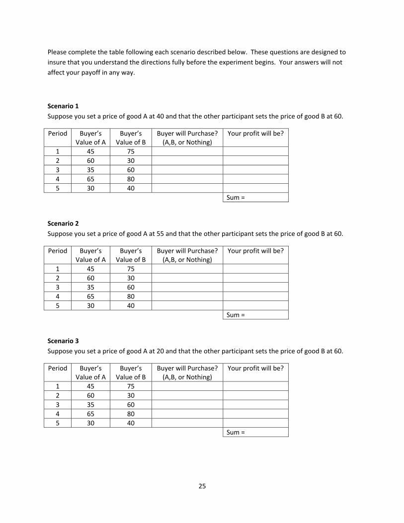
Please complete the table following each scenario described below. These questions are designed to
insure that you understand the directions fully before the experiment begins. Your answers will not
affect your payoff in any way.
Scenario 1
Suppose you set a price of good A at 40 and that the other participant sets the price of good B at 60.
Period Buyer’s Value of A
Buyer’s Value of B
Buyer will Purchase? (A,B, or Nothing)
Your profit will be?
1 45 75
2 60 30
3 35 60
4 65 80
5 30 40
Sum =
Scenario 2
Suppose you set a price of good A at 55 and that the other participant sets the price of good B at 60.
Period Buyer’s Value of A
Buyer’s Value of B
Buyer will Purchase? (A,B, or Nothing)
Your profit will be?
1 45 75
2 60 30
3 35 60
4 65 80
5 30 40
Sum =
Scenario 3
Suppose you set a price of good A at 20 and that the other participant sets the price of good B at 60.
Period Buyer’s Value of A
Buyer’s Value of B
Buyer will Purchase? (A,B, or Nothing)
Your profit will be?
1 45 75
2 60 30
3 35 60
4 65 80
5 30 40
Sum =
Economic Science Institute Working Papers
2010
10-12 Kovenock, D., Roberson, B.,and Sheremeta, R. The Attack and Defense of Weakest-Link Networks.
10-11 Wilson, B., Jaworski, T., Schurter, K. and Smyth, A. An Experimental Economic History of Whalers’ Rules of Capture.
10-10 DeScioli, P. and Wilson, B. Mine and Thine: The Territorial Foundations of Human Property.
10-09 Cason, T., Masters, W. and Sheremeta, R. Entry into Winner-Take-All and Proportional-Prize Contests: An Experimental Study.
10-08 Savikhin, A. and Sheremeta, R. Simultaneous Decision-Making in Competitive and Cooperative Environments.
10-07 Chowdhury, S. and Sheremeta, R. A generalized Tullock contest. 10-06 Chowdhury, S. and Sheremeta, R. The Equivalence of Contests. 10-05 Shields, T. Do Analysts Tell the Truth? Do Shareholders Listen? An Experimental Study of Analysts' Forecasts and Shareholder Reaction. 10-04 Lin, S. and Rassenti, S. Are Under- and Over-reaction the Same Matter? A Price Inertia based Account. 10-03 Lin, S. Gradual Information Diffusion and Asset Price Momentum. 10-02 Gjerstad, S. and Smith, V. Household expenditure cycles and economic cycles, 1920 – 2010. 10-01 Dickhaut, J., Lin, S., Porter, D. and Smith, V. Durability, Re-trading and Market Performance.
2009
09-11 Hazlett, T., Porter, D., Smith, V. Radio Spectrum and the Disruptive Clarity OF Ronald Coase. 09-10 Sheremeta, R. Expenditures and Information Disclosure in Two-Stage Political Contests. 09-09 Sheremeta, R. and Zhang, J. Can Groups Solve the Problem of Over-Bidding in Contests? 09-08 Sheremeta, R. and Zhang, J. Multi-Level Trust Game with "Insider" Communication. 09-07 Price, C. and Sheremeta, R. Endowment Effects in Contests. 09-06 Cason, T., Savikhin, A. and Sheremeta, R. Cooperation Spillovers in Coordination Games. 09-05 Sheremeta, R. Contest Design: An Experimental Investigation.
09-04 Sheremeta, R. Experimental Comparison of Multi-Stage and One-Stage Contests. 09-03 Smith, A., Skarbek, D., and Wilson, B. Anarchy, Groups, and Conflict: An Experiment on the Emergence of Protective Associations.
09-02 Jaworski, T. and Wilson, B. Go West Young Man: Self-selection and Endogenous Property Rights.
09-01 Gjerstad, S. Housing Market Price Tier Movements in an Expansion and Collapse.
2008
08-10 Dickhaut, J., Houser, D., Aimone, J., Tila, D. and Johnson, C. High Stakes Behavior with Low Payoffs: Inducing Preferences with Holt-Laury Gambles.
08-09 Stecher, J., Shields, T. and Dickhaut, J. Generating Ambiguity in the Laboratory.
08-08 Stecher, J., Lunawat, R., Pronin, K. and Dickhaut, J. Decision Making and Trade without Probabilities.
08-07 Dickhaut, J., Lungu, O., Smith, V., Xin, B. and Rustichini, A. A Neuronal Mechanism of Choice.
08-06 Anctil, R., Dickhaut, J., Johnson, K., and Kanodia, C. Does Information Transparency Decrease Coordination Failure?
08-05 Tila, D. and Porter, D. Group Prediction in Information Markets With and Without Trading Information and Price Manipulation Incentives.
08-04 Caginalp, G., Hao, L., Porter, D. and Smith, V. Asset Market Reactions to News: An Experimental Study.
08-03 Thomas, C. and Wilson, B. Horizontal Product Differentiation in Auctions and Multilateral Negotiations.
08-02 Oprea, R., Wilson, B. and Zillante, A. War of Attrition: Evidence from a Laboratory Experiment on Market Exit.
08-01 Oprea, R., Porter, D., Hibbert, C., Hanson, R. and Tila, D. Can Manipulators Mislead Prediction Market Observers?