Comparison of Discrete Curvature Estimatorsand Application to Corner Detection

B. Kerautret1, J.-O. Lachaud2, and B. Naegel1,�

1 LORIA, Nancy-University - IUT de Saint Die des Vosges54506 Vandœuvre -les-Nancy Cedex

{kerautre,naegelbe}@loria.fr2 LAMA, University of Savoie

73376 Le Bourget du Lacjacques-olivier.lachaud@univ-savoie.fr

Abstract. Several curvature estimators along digital contours were pro-posed in recent works [1,2,3]. These estimators are adapted to non per-fect digitization process and can process noisy contours. In this paper,we compare and analyse the performances of these estimators on severaltypes of contours and we measure execution time on both perfect andnoisy shapes. In a second part, we evaluate these estimators in the con-text of corner detection. Finally to evaluate the performance of a noncurvature based approach, we compare the results with a morphologicalcorner detector [4].

1 Introduction

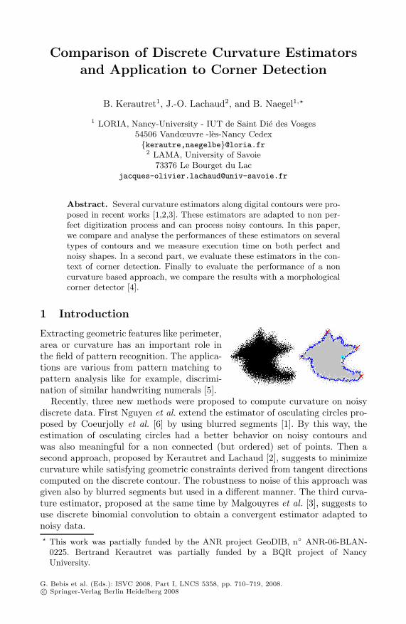
Extracting geometric features like perimeter,area or curvature has an important role inthe field of pattern recognition. The applica-tions are various from pattern matching topattern analysis like for example, discrimi-nation of similar handwriting numerals [5].

Recently, three new methods were proposed to compute curvature on noisydiscrete data. First Nguyen et al. extend the estimator of osculating circles pro-posed by Coeurjolly et al. [6] by using blurred segments [1]. By this way, theestimation of osculating circles had a better behavior on noisy contours andwas also meaningful for a non connected (but ordered) set of points. Then asecond approach, proposed by Kerautret and Lachaud [2], suggests to minimizecurvature while satisfying geometric constraints derived from tangent directionscomputed on the discrete contour. The robustness to noise of this approach wasgiven also by blurred segments but used in a different manner. The third curva-ture estimator, proposed at the same time by Malgouyres et al. [3], suggests touse discrete binomial convolution to obtain a convergent estimator adapted tonoisy data.� This work was partially funded by the ANR project GeoDIB, n◦ ANR-06-BLAN-

0225. Bertrand Kerautret was partially funded by a BQR project of NancyUniversity.

G. Bebis et al. (Eds.): ISVC 2008, Part I, LNCS 5358, pp. 710–719, 2008.c© Springer-Verlag Berlin Heidelberg 2008

Comparison of Discrete Curvature Estimators 711

In this work, we propose to evaluate experimentally these three estimators byusing different test contours and by measuring the precision of the estimationwith several grid sizes. After comparing the curvature obtained with low andlarge resolution, we measure the robustness of the estimator on noisy contours.A second objective of this paper is to apply the most stable and robust of theseestimators to a concrete application of corner detection (see the previous figure).Moreover we compare the obtained results with a recent morphological cornerdetector [4].

This paper is organized as follows. In the following section, after introducingbriefly some notions of digital blurred segments, we give a rapid descriptionof the three estimators. Then the comparison of these estimators is given insection 3. Section 4 shows the application to corner detection and describes thecomparative evaluation.

2 Discrete Curvature Estimators

Before describing the curvature estimators previously mentioned, we address thenotion of digital blurred segments used by the two first estimators.

Blurred segments were introduced by Debled et al. [7]. Note that a comparablealgorithm was proposed by Buzer [8]. The notion of blurred segments is basedon the arithmetic definition of digital straight line and uses the computation ofthe convex hull to determine its vertical geometric width ν. From this definitionthe authors proposed an algorithm for the recognition of blurred segments ofwidth ν. Note that the two following curvature estimators use the version of thealgorithm which is not restricted to the hypothesis that points are added withincreasing x coordinate (or y coordinate). The next floating figure illustrates twoblurred segments of width 5 computed from the central black pixel.

2.1 Estimator Based on Osculating Circles (CC and NDC)

The curvature estimator proposed by Nguyen andR

BS(l, k) BS(k, r)

Debled-Rennesson [7] follows the same concept thanthe estimator proposed by Coeurjolly et al. [6] (calledCC estimator). The latter is based on the estimationof osculating circles. More precisely, by denoting Ca discrete curve, Ci,j the sequence of points goingfrom Ci to Cj and BSν(i, j) the predicate “Ci,j is ablurred segment of width ν”. We consider the points Cr and Cl defined suchthat: BSν(l, k) ∧ ¬BSν(l − 1, k) ∧ BSν(k, r) ∧ ¬BSν(k, r + 1). With this defini-tion, they determine the curvature of width ν at the point Ck from the radius ofthe circle passing through Ck, Cl and Cr . By noting s1 = ||−−−→

CkCr||, s2 = ||−−−→CkCl||

and s3 = ||−−−→ClCr||, the authors give the following expression of radius Rν of the

circle associated to the point Ck:

Rν(Ck) =s1s2s3√

(s1 + s2 + s3)(s1 − s2 + s3)(s1 + s2 − s3)(s2 + s3 − s1)

712 B. Kerautret, J.-O. Lachaud, and B. Naegel

If the vectors−−−→CkCl and

−−−→CkCl are not collinear then the curvature of width ν can

be determined with sign(det(−−−−−−−−→CkCr,CkCl))

Rν(Ck) . Otherwise the curvature is set to 0.

2.2 Global Minimization Curvature Estimator (GMC)

The estimator proposed by Kerautret and Lachaud is based on two main ideas [2].The first one is to take into account all the possible shapes that have the samedigitization defined by the initial contour and to select the most probable con-tour. This selection is done with a global optimization by minimizing the squaredcurvature. From this idea, we can expect a precise result even with a low contourresolution. The second idea is to obtain an estimator not sensitive to noise or tonon perfect digitization process with blurred segments.

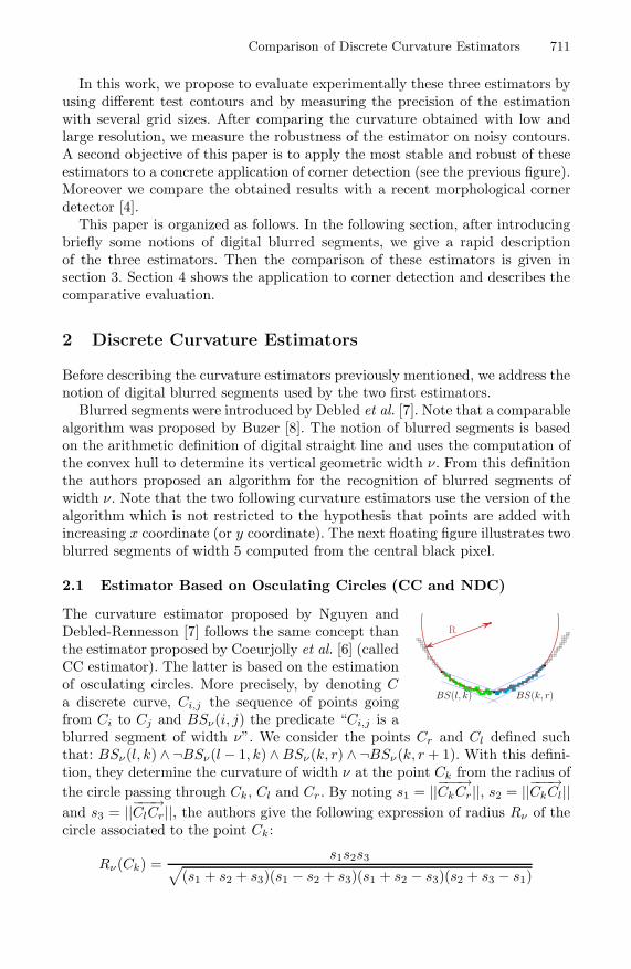
For the purpose of minimizing curvature, the tangentialcover [9] is computed on the discrete contour and the minimaland maximal possible tangent values are defined for each pixel.Fig. 1 illustrates both tangential cover (a) and bounds on thetangent directions (b). Minimizing the curvature consists inmoving each point (xi, yi) along the y axis and between thebounds defined by ymin, ymax in order to minimize the slopeof the line joining (xi, yi) to (xi+1, yi+1). The global minimization is applied witha relaxation process.

For the robustness to noise and non perfect digitization process, the discretemaximal segments were replaced by the discrete maximal blurred segments pre-viously described. Note that the definition of the minimal and maximal slopesof the blurred segments is notably different from the non blurred case (see [2]for more details).

0

1

2

3

4

5

6

7

8

9

0 10 20 30 40 50 60 70

Bounds on tangent directionsYminYmax

0

1

2

3

4

5

6

7

8

9

0 10 20 30 40 50 60 70

Constraints for each variableYminYmax

(a) (b)

Fig. 1. Illustration of bounds defined from maximal segments (a) (extracted from theprevious floating figure). (b) shows the constraints defined on each variable.

2.3 Binomial Convolution Curvature Estimator (BCC)

Malgouyres et al. proposed an algorithm to estimate derivatives with binomialconvolutions [3] which is claimed to be multigrid convergent. They define the

Comparison of Discrete Curvature Estimators 713

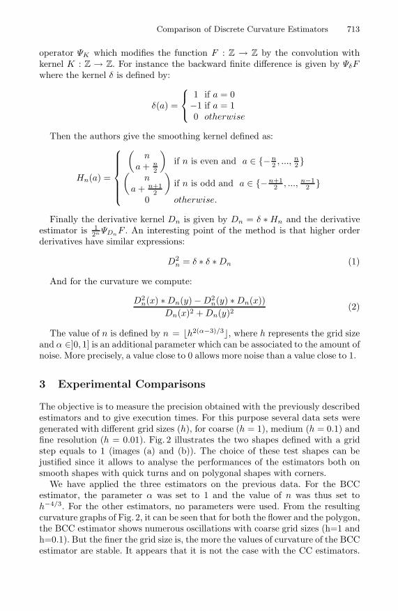
operator ΨK which modifies the function F : Z → Z by the convolution withkernel K : Z → Z. For instance the backward finite difference is given by ΨδFwhere the kernel δ is defined by:

δ(a) =

⎧⎨

⎩

1 if a = 0−1 if a = 10 otherwise

Then the authors give the smoothing kernel defined as:

Hn(a) =

⎧⎪⎪⎪⎪⎨

⎪⎪⎪⎪⎩

(n

a + n2

)if n is even and a ∈ {−n

2 , ..., n2 }

(n

a + n+12

)if n is odd and a ∈ {−n+1

2 , ..., n−12 }

0 otherwise.

Finally the derivative kernel Dn is given by Dn = δ ∗ Hn and the derivativeestimator is 1

2n ΨDnF . An interesting point of the method is that higher orderderivatives have similar expressions:

D2n = δ ∗ δ ∗ Dn (1)

And for the curvature we compute:

D2n(x) ∗ Dn(y) − D2

n(y) ∗ Dn(x))Dn(x)2 + Dn(y)2

(2)

The value of n is defined by n = �h2(α−3)/3�, where h represents the grid sizeand α ∈]0, 1] is an additional parameter which can be associated to the amount ofnoise. More precisely, a value close to 0 allows more noise than a value close to 1.

3 Experimental Comparisons

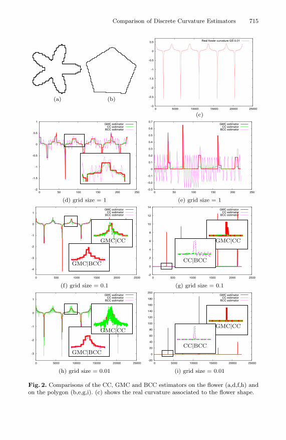
The objective is to measure the precision obtained with the previously describedestimators and to give execution times. For this purpose several data sets weregenerated with different grid sizes (h), for coarse (h = 1), medium (h = 0.1) andfine resolution (h = 0.01). Fig. 2 illustrates the two shapes defined with a gridstep equals to 1 (images (a) and (b)). The choice of these test shapes can bejustified since it allows to analyse the performances of the estimators both onsmooth shapes with quick turns and on polygonal shapes with corners.

We have applied the three estimators on the previous data. For the BCCestimator, the parameter α was set to 1 and the value of n was thus set toh−4/3. For the other estimators, no parameters were used. From the resultingcurvature graphs of Fig. 2, it can be seen that for both the flower and the polygon,the BCC estimator shows numerous oscillations with coarse grid sizes (h=1 andh=0.1). But the finer the grid size is, the more the values of curvature of the BCCestimator are stable. It appears that it is not the case with the CC estimators.

714 B. Kerautret, J.-O. Lachaud, and B. Naegel

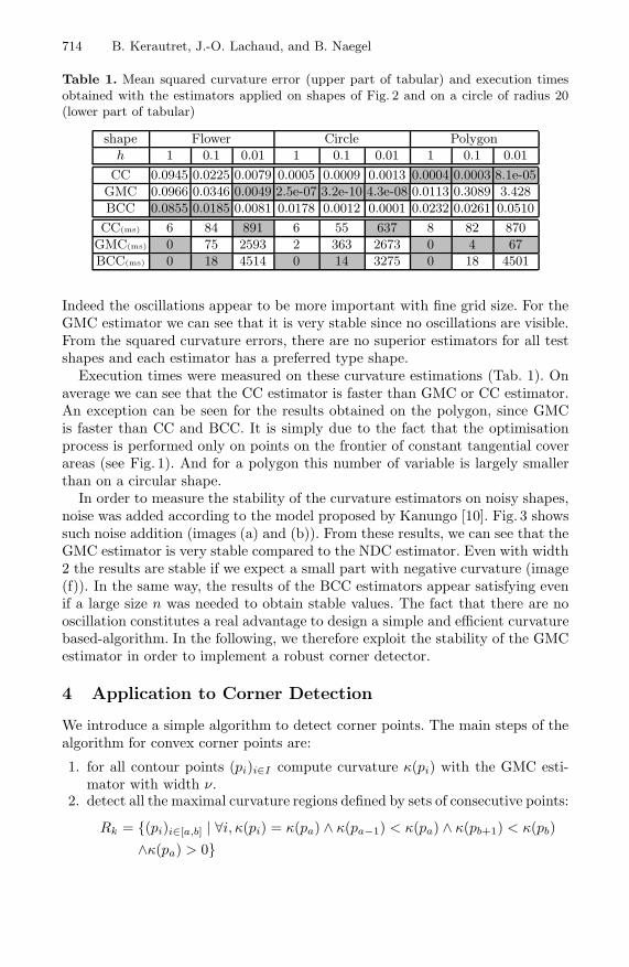
Table 1. Mean squared curvature error (upper part of tabular) and execution timesobtained with the estimators applied on shapes of Fig. 2 and on a circle of radius 20(lower part of tabular)

shape Flower Circle Polygonh 1 0.1 0.01 1 0.1 0.01 1 0.1 0.01

CC 0.0945 0.0225 0.0079 0.0005 0.0009 0.0013 0.0004 0.0003 8.1e-05GMC 0.0966 0.0346 0.0049 2.5e-07 3.2e-10 4.3e-08 0.0113 0.3089 3.428BCC 0.0855 0.0185 0.0081 0.0178 0.0012 0.0001 0.0232 0.0261 0.0510

CC(ms) 6 84 891 6 55 637 8 82 870GMC(ms) 0 75 2593 2 363 2673 0 4 67BCC(ms) 0 18 4514 0 14 3275 0 18 4501

Indeed the oscillations appear to be more important with fine grid size. For theGMC estimator we can see that it is very stable since no oscillations are visible.From the squared curvature errors, there are no superior estimators for all testshapes and each estimator has a preferred type shape.

Execution times were measured on these curvature estimations (Tab. 1). Onaverage we can see that the CC estimator is faster than GMC or CC estimator.An exception can be seen for the results obtained on the polygon, since GMCis faster than CC and BCC. It is simply due to the fact that the optimisationprocess is performed only on points on the frontier of constant tangential coverareas (see Fig. 1). And for a polygon this number of variable is largely smallerthan on a circular shape.

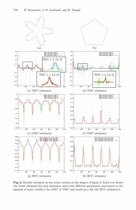
In order to measure the stability of the curvature estimators on noisy shapes,noise was added according to the model proposed by Kanungo [10]. Fig. 3 showssuch noise addition (images (a) and (b)). From these results, we can see that theGMC estimator is very stable compared to the NDC estimator. Even with width2 the results are stable if we expect a small part with negative curvature (image(f)). In the same way, the results of the BCC estimators appear satisfying evenif a large size n was needed to obtain stable values. The fact that there are nooscillation constitutes a real advantage to design a simple and efficient curvaturebased-algorithm. In the following, we therefore exploit the stability of the GMCestimator in order to implement a robust corner detector.

4 Application to Corner Detection

We introduce a simple algorithm to detect corner points. The main steps of thealgorithm for convex corner points are:

1. for all contour points (pi)i∈I compute curvature κ(pi) with the GMC esti-mator with width ν.

2. detect all the maximal curvature regions defined by sets of consecutive points:

Rk = {(pi)i∈[a,b] | ∀i, κ(pi) = κ(pa) ∧ κ(pa−1) < κ(pa) ∧ κ(pb+1) < κ(pb)∧κ(pa) > 0}

Comparison of Discrete Curvature Estimators 715

(a) (b)-3

-2.5

-2

-1.5

-1

-0.5

0

0.5

0 5000 10000 15000 20000 25000

Real flower curvature GS 0.01

(c)

-2

-1.5

-1

-0.5

0

0.5

1

0 50 100 150 200 250

GMC estimatorCC estimator

BCC estimator

-0.3

-0.2

-0.1

0

0.1

0.2

0.3

0.4

0.5

0.6

0.7

0 50 100 150 200 250

GMC estimatorCC estimator

BCC estimator

(d) grid size = 1 (e) grid size = 1

-4

-3

-2

-1

0

1

0 500 1000 1500 2000 2500

GMC estimatorCC estimator

BCC estimator

GMC|CC

GMC|BCC

-2

0

2

4

6

8

10

12

14

0 500 1000 1500 2000 2500

GMC estimatorCC estimator

BCC estimator

GMC|CC

CC|BCC

(f) grid size = 0.1 (g) grid size = 0.1

-3

-2

-1

0

1

0 5000 10000 15000 20000 25000

GMC estimatorCC estimator

BCC estimator

GMC|CC

GMC|BCC-20

0

20

40

60

80

100

120

140

160

180

200

0 5000 10000 15000 20000 25000

GMC estimatorCC estimator

BCC estimator

GMC|CC

CC|BCC

(h) grid size = 0.01 (i) grid size = 0.01

Fig. 2. Comparisons of the CC, GMC and BCC estimators on the flower (a,d,f,h) andon the polygon (b,e,g,i). (c) shows the real curvature associated to the flower shape.

716 B. Kerautret, J.-O. Lachaud, and B. Naegel

(a) (b)

-0.4

-0.3

-0.2

-0.1

0

0.1

0.2

0.3

0.4

0 200 400 600 800 1000 1200

NDC estimator width=2NDC estimator width=3NDC estimator width=4

NDC ν = {2, 3}

NDC ν = {3, 4}

-0.4

-0.3

-0.2

-0.1

0

0.1

0.2

0.3

0.4

0 200 400 600 800 1000 1200

NDC estimator width=2NDC estimator width=3NDC estimator width=4

NDC ν = {3, 4}

(c) NDC estimator (d) NDC estimator

-0.25

-0.2

-0.15

-0.1

-0.05

0

0.05

0.1

0 200 400 600 800 1000 1200

GMC estimator width=2GMC estimator width=3GMC estimator width=4

-0.02

0

0.02

0.04

0.06

0.08

0.1

0.12

0.14

0 200 400 600 800 1000 1200

GMC estimator width=2GMC estimator width=3GMC estimator width=4

(e) GMC estimator (f) GMC estimator

-0.14

-0.12

-0.1

-0.08

-0.06

-0.04

-0.02

0

0.02

0.04

0.06

0 200 400 600 800 1000 1200

BCC estimator mask size=200BCC estimator mask size=300BCC estimator mask size=400

-0.01

0

0.01

0.02

0.03

0.04

0.05

0.06

0 200 400 600 800 1000 1200

BCC estimator mask size=200BCC estimator mask size=300BCC estimator mask size=400

(g) BCC estimator (h) BCC estimator

Fig. 3. Results obtained on the noisy version on the shapes of figure 2. Each row showsthe result obtained for each estimator used with different parameters associated to theamount of noise (width ν for GMC et NDC and mask size for the BCC estimator).

Comparison of Discrete Curvature Estimators 717

3. for each region Rk mark the point p(a+b)/2 as a corner.4. (optional) select only corner points with curvature bigger than a threshold

value κmin.

Note that a quantification of the curvature field was applied in order to simplifythe detection of the local minima/maxima (set to 1e−3). In the rest of this paperwe have not applied the optional step (4) since it adds a new parameter and itcould be fixed for each particular application. The concave corner detection isdeduced by replacing the maximal by the minimal curvature regions.

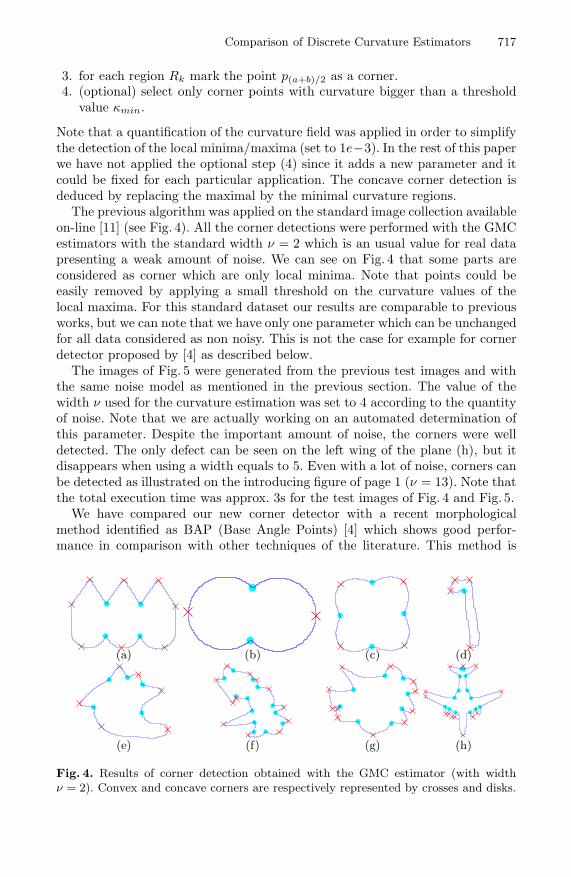
The previous algorithm was applied on the standard image collection availableon-line [11] (see Fig. 4). All the corner detections were performed with the GMCestimators with the standard width ν = 2 which is an usual value for real datapresenting a weak amount of noise. We can see on Fig. 4 that some parts areconsidered as corner which are only local minima. Note that points could beeasily removed by applying a small threshold on the curvature values of thelocal maxima. For this standard dataset our results are comparable to previousworks, but we can note that we have only one parameter which can be unchangedfor all data considered as non noisy. This is not the case for example for cornerdetector proposed by [4] as described below.

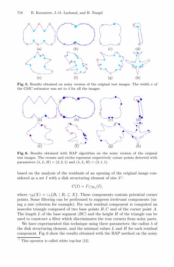
The images of Fig. 5 were generated from the previous test images and withthe same noise model as mentioned in the previous section. The value of thewidth ν used for the curvature estimation was set to 4 according to the quantityof noise. Note that we are actually working on an automated determination ofthis parameter. Despite the important amount of noise, the corners were welldetected. The only defect can be seen on the left wing of the plane (h), but itdisappears when using a width equals to 5. Even with a lot of noise, corners canbe detected as illustrated on the introducing figure of page 1 (ν = 13). Note thatthe total execution time was approx. 3s for the test images of Fig. 4 and Fig. 5.

We have compared our new corner detector with a recent morphologicalmethod identified as BAP (Base Angle Points) [4] which shows good perfor-mance in comparison with other techniques of the literature. This method is

(a) (b) (c) (d)

(e) (f) (g) (h)

Fig. 4. Results of corner detection obtained with the GMC estimator (with widthν = 2). Convex and concave corners are respectively represented by crosses and disks.

718 B. Kerautret, J.-O. Lachaud, and B. Naegel

(a) (b) (c) (d)

(e) (f) (g) (h)

Fig. 5. Results obtained on noisy version of the original test images. The width ν ofthe GMC estimator was set to 4 for all the images.

(a) (b) (c) (d)

(e) (f) (g) (h)

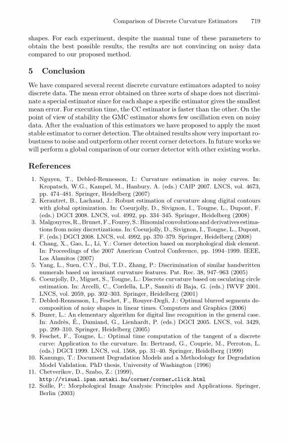
Fig. 6. Results obtained with BAP algorithm on the noisy version of the originaltest images. The crosses and circles represent respectively corner points detected withparameters (λ, L, H) = (2, 2, 1) and (λ, L, H) = (3, 1, 1).

based on the analysis of the residuals of an opening of the original image con-sidered as a set I with a disk structuring element of size λ1:

C(I) = I\γBλ(I),

where γB(X) = ∪i{Bi | Bi ⊆ X}. These components contain potential cornerpoints. Some filtering can be performed to suppress irrelevant components (us-ing a size criterion for example). For each residual component is computed anisosceles triangle composed of two base points B, C and of the corner point A.The length L of the base segment |BC| and the height H of the triangle can beused to construct a filter which discriminates the true corners from noisy parts.

We have experimented this technique using three parameters: the radius λ ofthe disk structuring element, and the minimal values L and H for each residualcomponent. Fig. 6 show the results obtained with the BAP method on the noisy1 This operator is called white top-hat [12].

Comparison of Discrete Curvature Estimators 719

shapes. For each experiment, despite the manual tune of these parameters toobtain the best possible results, the results are not convincing on noisy datacompared to our proposed method.

5 Conclusion

We have compared several recent discrete curvature estimators adapted to noisydiscrete data. The mean error obtained on three sorts of shape does not discrimi-nate a special estimator since for each shape a specific estimator gives the smallestmean error. For execution time, the CC estimator is faster than the other. On thepoint of view of stability the GMC estimator shows few oscillation even on noisydata. After the evaluation of this estimators we have proposed to apply the moststable estimator to corner detection. The obtained results show very important ro-bustness to noise and outperform other recent corner detectors. In future works wewill perform a global comparison of our corner detector with other existing works.

References

1. Nguyen, T., Debled-Rennesson, I.: Curvature estimation in noisy curves. In:Kropatsch, W.G., Kampel, M., Hanbury, A. (eds.) CAIP 2007. LNCS, vol. 4673,pp. 474–481. Springer, Heidelberg (2007)

2. Kerautret, B., Lachaud, J.: Robust estimation of curvature along digital contourswith global optimization. In: Coeurjolly, D., Sivignon, I., Tougne, L., Dupont, F.(eds.) DGCI 2008. LNCS, vol. 4992, pp. 334–345. Springer, Heidelberg (2008)

3. Malgouyres,R.,Brunet, F., Fourey, S.:Binomial convolutions andderivatives estima-tions from noisy discretizations. In: Coeurjolly, D., Sivignon, I., Tougne, L., Dupont,F. (eds.) DGCI 2008. LNCS, vol. 4992, pp. 370–379. Springer, Heidelberg (2008)

4. Chang, X., Gao, L., Li, Y.: Corner detection based on morphological disk element.In: Proceedings of the 2007 American Control Conference, pp. 1994–1999. IEEE,Los Alamitos (2007)

5. Yang, L., Suen, C.Y., Bui, T.D., Zhang, P.: Discrimination of similar handwrittennumerals based on invariant curvature features. Pat. Rec. 38, 947–963 (2005)

6. Coeurjolly, D., Miguet, S., Tougne, L.: Discrete curvature based on osculating circleestimation. In: Arcelli, C., Cordella, L.P., Sanniti di Baja, G. (eds.) IWVF 2001.LNCS, vol. 2059, pp. 302–303. Springer, Heidelberg (2001)

7. Debled-Rennesson, I., Feschet, F., Rouyer-Degli, J.: Optimal blurred segments de-composition of noisy shapes in linear times. Computers and Graphics (2006)

8. Buzer, L.: An elementary algorithm for digital line recognition in the general case.In: Andres, E., Damiand, G., Lienhardt, P. (eds.) DGCI 2005. LNCS, vol. 3429,pp. 299–310. Springer, Heidelberg (2005)

9. Feschet, F., Tougne, L.: Optimal time computation of the tangent of a discretecurve: Application to the curvature. In: Bertrand, G., Couprie, M., Perroton, L.(eds.) DGCI 1999. LNCS, vol. 1568, pp. 31–40. Springer, Heidelberg (1999)

10. Kanungo, T.: Document Degradation Models and a Methodology for DegradationModel Validation. PhD thesis, University of Washington (1996)

11. Chetverikov, D., Szabo, Z.: (1999),http://visual.ipan.sztaki.hu/corner/corner click.html

12. Soille, P.: Morphological Image Analysis: Principles and Applications. Springer,Berlin (2003)