Comparing the performance of open loop centroiding ...web.uvic.ca/~ravenmoa/Docs/Andersen_SPIE_2014.pdf · Comparing the performance of open loop centroiding techniques in the Raven

Comparing the performance of open loop centroiding techniques in the Raven MOAO system

David R. Andersen*a, Colin Bradleyb, Darryl Gamrothb, Dan Kerleya, Olivier Lardièreb, Jean-Pierre

Vérana

aNRC Herzberg Astronomy, 5071 W. Saanich Rd, Victoria, BC, CANADA V8X-2G6; bDept. of Mechanical Engineering, University of Victoria, 3800 Finnerty Rd., Victoria, BC

CANADA

ABSTRACT

Raven is a multi-object adaptive optics (MOAO) demonstrator that will be mounted on the NIR Nasmyth platform of the Subaru telescope in May, 2014. Raven can use three open-loop NGS WFSs and an on-axis LGS WFS to control DMs in two separate science pick-off arms. Centroiding in open loop AO systems like Raven is more difficult than in closed loop AO systems because the Shack-Hartmann spots will not be driven to the same spot on a detector. Rather the spots can fall on any combination of pixels because the WFSs need to have sufficient dynamic range to measure the full turbulence. In this paper, we compare correlation and thresholded center of gravity (tCOG) centroiding methods in simulation, with Raven using its calibration unit, and on-sky. Each method has its own advantages. Correlation centroiding is superior to tCOG centroiding for faint NGSs and for extended sources (Raven open loop WFSs do not contain ADCs so spots will become elongated). We expect that correlation centroiding will push the limiting magnitude of Raven NGSs fainter by roughly one magnitude. Correlation centroiding is computationally more intensive, however, and actually will limit Raven’s sampling rate for shorter integrations. Therefore, for bright stars with sufficiently high signal-to-noise, Raven can be run significantly faster and with superior performance using the tCOG method. Here we quantify both the performance and timing differences of these two centroiding methods in simulation, in the lab and on sky using Raven.

Keywords: Astronomical Instrumentation; Adaptive Optics (AO); Multi-Object Adaptive Optics (MOAO); Wavefront Sensing Techniques

1. INTRODUCTION Multi-Object Adaptive Optics (MOAO)1 systems of the future will deliver diffraction-limited images over a large field of regard (FoR). On Extremely Large Telescopes (ELTs) with multiple Laser Guide Stars (LGSs), a MOAO-fed instrument with at least 20 science pick-offs spread over a FoR of at least 5 arcminutes should deliver 50% ensquared energy (EE) within a 50 milli-arcsecond spaxel in H-band over 90% of the sky. With this potentially impressive performance and large multiplexing advantage, MOAO instruments should be work-horse instruments on ELTs2,3,4. However, before serious design work can proceed on these future ELT instruments, the technical risks associated with this novel AO concept must be mitigated. The community has responded with a series of increasingly complex on-sky demonstrators,5,6 most notably, Canary7.

Raven is the first MOAO science demonstrator on an 8 m-class telescope8. It recently saw first light on the Subaru telescope on May 13 and 14, 2014. Raven contains six wavefront sensors (WFSs): Three WFSs are open-loop natural guide star (NGS) WFSs that are used to sense the volume of turbulence above the telescope. Signal from these three NGS WFSs can be augmented by a WFS sensing light from the on-axis Subaru LGS. After creating a tomographic model of the atmosphere9 using the signal from three or four WFSs, the optimal correction can be calculated and applied in the direction of any two science objects in the FoR. Light from the science objects is picked-off by two science arms. Two Deformable Mirrors (DMs) embedded in each science channel apply the correction. Two closed-loop WFSs located behind the DMs are used for calibration purposes and truth wavefront sensing. The light from the two science

* [email protected]; phone 1 250 363-8708; fax 1 250 363-0045; www.nrc-cnrc.gc.ca/eng/rd/nsi/

Adaptive Optics Systems IV, edited by Enrico Marchetti, Laird M. Close, Jean-Pierre Véran, Proc. of SPIE Vol. 9148, 91485K · © 2014 SPIE

CCC code: 0277-786X/14/$18 · doi: 10.1117/12.2057160

Proc. of SPIE Vol. 9148 91485K-1

Downloaded From: http://proceedings.spiedigitallibrary.org/ on 02/04/2015 Terms of Use: http://spiedl.org/terms

channgls are combined and can be re-imaged either onto IRCS10, the Subaru facility imaging spectrograph, or onto a Raven InGaAs “science” detector.

For Raven to be effective as a MOAO science demonstrator, it needs to have non-negligible sky coverage. Because Raven relies on two or (usually) three open loop NGS WFSs while operating in MOAO mode, decisions were made to make Raven operate with even relatively faint stars thereby improving sky coverage. This effort impacted the AO architecture11, the design12, and guided our work in developing optimal reconstruction techniques13 and open loop centroiding algorithms.

In this paper, we explore the performance of thresholded-center of gravity (tCOG) and correlation centroiding algorithms in open-loop. In closed-loop, it is known that tCOG is computationally efficient while correlation centroiding takes more computational power but yields more accurate slopes14,15. Matched Filter centroiding16 performs almost as well as correlation centroiding in closed-loop and is computationally efficient, but this technique lacks sufficient dynamic range for use in open loop MOAO systems where the spots are not driven toward their reference locations by a closed loop DM. Therefore, we first simulate the accuracy of tCOG and correlation centroiding using Monte Carlo simulations to determine whether Raven will see sufficient gains to warrant including correlation centroiding in the pixel processing pipeline of the Raven Real Time Computer (RTC). Having established that correlation centroiding is worth including, we then compare tCOG and correlation centroiding results for Raven from both the lab and on-sky.

Before proceeding to a discussion of open-loop centroiding, it is important to note the limitations of the Raven WFSs. We are using the Andor iXon cameras with 128x128 pixels. As part of our trade study, we determined that we need a roughly 5 arcsec FOV and at least 10x10 subapertures to achieve the dynamic range and sensitivity, respectively, to achieve the overall system requirements. This means that there are only going to be ~12x12 pixels per subaperture and that the pixel size needs to be ~0.4 arsec/pixel. Since the spot size on the WFS will most often be smaller than 0.8, that means that the spots will be under-sampled. As we showed in Andersen et al.11, we expect a 70 nm wavefront error (WFE) due to this under-sampling, but this will be centroiding algorithm dependent. Here we determine which centroiding algorithm works best at both high and low S/N.

Section 2 describes simulations carried out to test the sensitivity of tCOG and correlation open-loop centroiding algorithms in the context of the Raven. We present centroiding test results obtained from Raven in the lab in section 3. Section 4 describes work done using WFS frames obtained during Raven’s first light run. We summarize our work in section 5.

2. OPEN LOOP CENTROIDING SIMULATIONS We performed our open-loop centroiding simulations in matlab using the UVic AO library. The goal of these simulations was to assess the amount of extra WFE and loss in EE due to aliasing, sampling error, and WFS noise (isolated from tomographic, DM fitting and temporal errors) when using tCOG or correlation algorithms.

The tCOG centroiding algorithm is the simplest method and is computationally fast. In our flux-threshold variant of tCOG, the maximum flux is determined in each subaperture and only those pixels with a flux above some percentage of the peak flux (usually 20%) would be used for determining a flux-weighted mean. We also use a minimum threshold which is set to remove background and readnoise, even if this level is greater than the threshold determined from the peak flux. Correlation centroiding relies on knowledge of the spot image. In section 2.1, we describe how we generate a reference WFS spot image from our measurements and then correlate our WFS spot images with this reference image. This correlation process creates a new image for each subaperture that enhances features in the frame that have a similar shape to the reference image while smoothing away structure that does not look like the reference image (e.g., shot noise and cosmic rays). The centroid can be determined from the correlation image using the tCOG with a relatively high threshold.

2.1 Method

We began by simulating 200 independent phase screens with a Fried parameter of r0=15 cm and a sampling of 0.017 m. For each of these phase screens, we simulated spots in 80 0.8x0.8 m2 subapertures with a pixel sampling of 0.1 arcsec/pixel and a FOV of 4.8 arcsec/subaperture. These spots are simulated with no noise initially. We can then bin these spot images by 2, 3, or 4 pixels and then scale the flux and add noise to simulate stars on WFSs with different sampling and different brightnesses (Figure 1). We simulated stars with brightnesses corresponding to R=10 to R=15 and WFS integration times of 80 ms (125 Hz). We assumed A0 stars and assumed that the WFS received half the V-



-2

-1

o

1

2

-7 -1 II j

arc5ec4 C-IdS

J

-2

-1

o

1

2

j II 1

arc5ec4 r1dS

l

NJ

NJ

ares

econ

ds ,

,1

O 1

N

NJ

O

NJ

jO

i

N

band, all the R-band and half the I-band. The effective readnoise is just 0.23 electrons, but the low readnoise of the Andor iXon camera is achieved by applying a high gain and then “counting” photons with a penalty in the photon noise.

Figure 1: Left Panel: WFS spot for 1 subaperture sampled with 0.1 arcsec/pixel and not including noise. Right Panel: The same WFS spot as on the left is shown but now sampled with 0.4 arcsec/pixel detector and including realistic photon and read noise.

Once realistic WFS spot images have been produced, we can measure centroids using various algorithms including tCOG and correlation techniques described above. Correlation centroiding requires reference images (i0) to be constructed. We construct reference images from the simulated data. For the high resolution WFSs (WFS sampling of 0.1 or 0.2 arcsec/pixel), it is best to just shift and add each of the individual images (Figure 2). For most situations, we create only one reference image for the whole WFS. One may create a reference image for each individual subaperture to account for pupil edge diffraction and possible lenslet to lenslet variations, but we found for the case of interest to us (0.4 arcsec/pix sampling), that we expect these variations to be smaller than the differences due to pixel blurring. Producing one reference image for the whole WFS also will have the advantage of having a higher signal-to-noise. The exception to this approach is for the case of the LGS WFS where we will produce a single reference image for each subaperture that will accurately reflect the laser elongation in each subaperture. We find that there is a potential gain to be had by shifting and adding individual WFS spot images onto a finer plate scale (“drizzling;” Figure 2).

Figure 2: Reference image comparison. The Left Panel shows the reference image for a WFS with 0.1 arcsec/pixel sampling. Each spot for 200 phase screens has been shifted and added to a single frame. If the same process in done using a plate scale of 0.4 arcsec/pixel, one finds a reference image shown in the Central Panel. The Right Panel shows the reference image that can be measured from 0.4 arcsec/pixel spots “drizzled” to a 0.2 arcsec/pixel grid. Drizzling can effectively increase the spatial resolution of the reference spot by a factor of 2.



4

-4

-4 -2 0

meters

2 4

0.6

0.4

0.2

0

-0.2

-0.4

5 10 15 20 25 30 35 40

Zernike Mode

To evaluate the impact of noise and sampling on Raven WFE and EE, we compared the measurements of slopes against some fiducial measurement of phase. We create this fiducial by projecting each phase screen onto 44 Zernike polynomials. This representation of the phase screen removes any DM fitting error for the results, but still allows us to assess WFS aliasing (higher modes not measured by the WFS producing slope offsets that thereby increase lower order wavefront errors).

For each set of slopes measured from a phase screen (for a given magnitude/sampling/centroiding algorithm), we multiply the resultant slopes by a modal reconstructor. We then compare the fiducial modal representations of the phase screen to our noisy reconstructions (Figure 3). We use two performance metrics to evaluate the performance: the rms WFE difference between these two phase maps and the loss of EE in a 150 mas spaxel due only to aliasing, sampling and WFS noise.

Figure 3: Left Panel: Residual phase map between the perfect projection of 44 modes onto the original phase screen and the reconstructed shape from the WFS (including sampling, aliasing, and noise errors). The scale on the color bars is WFE in microns. Right Panel: Comparison of the mode amplitude estimates (blue for the projection, red for the estimate from correlation slopes). 2.2 Results

The results of the simulations show that both the tCOG and correlation centroiding algorithms perform well in general. Results are summarized in Table 1. The centroiding algorithm out-performed the tCOG for faint stars (it should be less susceptible to noise artifacts), and worked well for the worst sampling (0.4 arcsec/pixel, which is used in the Raven WFS; Figure 4).

Table 1: For different WFS pixel scales and centroiding methods, we present the WFE and EE loss for bright and faint NGSs including aliasing, WFS noise and WFS sampling errors.

Pixel Scale tCOG (15%) Correlation R=11 Star R=14 Star R=11 Star R=14 Star

0.1” 121 (88%) 202 (80%) 0.2” 121 (88%) 158 (84%) 116 (90%) 151 (86%) 0.3” 124 (88%) 164 (83%) 113 (90%) 150 (86%) 0.4” 136 (87%) 185 (80%) 122 (89%) 165 (83%)



arcseconds

0

arcseconds

1.5511

-2 0

arcseconds

ix-2 0

200

180

E

" 160

140

12011

e 0.9E

- 088 -nnc.

11.5 12 12.5 13 13.5 14 14.5 15

c 0.86 .m

Ir

............'..%.q"" -.

.......j

. 1 . . 1 . 1 . AL . i . . . . .

11.5 12 12_5 13 13.5 14 14.5 15

NGS R magnitude

Figure 4: Left Panel: WFS spot image for 0.1 arcsec/pixel scale and a faint star. Left-Center Panel: Same spot convolved with the reference image. The effective S/N of the spot has been increased many-fold. Center-Right Panel: Same spot sampled onto a 0.4 arcsec/pixel WFS. Right Panel: The same 0.4 arcsec/pixel spot convolved with the reference image. Again, the effective S/N has been greatly enhanced.

Since correlation centroiding works better in these simulations than tCOG, we set out to explore the errors introduced by having reference images that were are not well-matched to the “true” reference image. We therefore ran the same simulations described above, but with synthetic reference images with varying widths (Figure 5).

Figure 5: Wavefront Error (WFE; top) and H-band Ensuared Energy (bottom) versus NGS magnitude for reference images with FWHM of 1.2 arcsec (purple), 1.4 arcsec (blue), 1.8 arcsec (green), 2.3 arcsec (dashed yellow) and 2.8 arcsec (dashed red). The best fit reference image (produced through drizzling) had a FWHM of 1.8 arcsec.



06

o

-0.5

o -1

-1,5 "400 600

I I ,

I00 700

Wavelength (areseconcis)

800 000

As Figure 5 shows, there is an impact on performance if the reference image does not match the average size of the spot images. We find about a 7% loss in EE if the reference image underestimates the FWHM of the spot image by 65%. The correlation method is less sensitive to an over-estimation of the spot size. We record only a 3.5% loss in EE when the reference image is 1.5 times bigger than the measured spots. We believe this is the case because a narrow reference spot would magnify narrower noise peaks after correlation. The relative losses due to a mismatch in reference image to spot size decrease at faint magnitudes; Figure 5 shows only a 3.5% loss in EE for the same reference image that is 65% narrower than the spot images. This is because the dominant error becomes WFS noise. This result is good news for Raven because we can use (relatively broad) synthetic reference images for faint magnitude guide stars where it is not practical to create reference images with little loss in performance, and for brighter stars we can create reference images from the WFS data as described above.

2.3 Using Correlation Centroiding at High Airmass

Raven as designed does not include an Atmospheric Dispersion Corrector (ADC) in any of its WFSs. Originally, we intended to use Raven only down to a zenith angle of 45 degrees, but several interesting science cases with targets near the Galactic Center push Raven to be used with zenith angles greater than 60 degrees (>2 airmasses). As broadband light passes through the atmosphere it is refracted and point sources are dispersed into very low resolution spectra. Using a model of the atmosphere over Mauna Kea, we can model the effect of atmospheric dispersion (Figure 6).

Figure 6: Atmospheric Dispersion in arcseconds versus wavelength for 3 zenith angles: 30 degrees (blue), 45 degrees (green) and 60 degrees (red) for Mauna Kea.

Figure 7 shows that the amount of dispersion can be large (~2 arcseconds at 60 degrees zenith angle). Here we assess how the effect it will have on Raven performance and whether Raven would perform better if it had ADCs designed into the WFSs. The three options we looked into were: 1) do nothing. No ADC means no loss in throughput. Also for bright stars, one can imagine that with correlation centroiding that there would actually be an advantage to having an elongated guide star. 2) use a filter that cuts off light below 600 nm. This could have three potential advantages: it would decrease the amount of atmospheric diffraction a great deal (down to ~0.4 arcseconds at 60 degrees zenith angle), a filter with a 600 nm could remove all scattered Na beacon light (589 nm), and the sky background could be greatly reduced. The disadvantage of course would be that the WFS would receive much less light in total. Finally, 3) we could redesign the WFSs to include an ADC. There would be a small loss of light due to the extra optical surfaces, but almost all the light in the optical would be concentrated within the seeing-limited PSF. We expect that the ADC option would give the best performance at low S/N.



2

1

0

-1

-2

-2 -1 0

arcseconds

i 2

2

1

0

-1

-2

-2 -1 0

arcseconds

1 2

Modeling on the ADC performance is very similar to the process described above in Section 2.1, except that we simulate the spots corresponding to the same initial turbulence but imaged at different wavelengths. We simulated spots at wavelengths of 400, 500, 600, 700, 800, and 900 nm. We combine these spot images into a single WFS frame by shifting single wavelength images using the dispersion corresponding to zenith angles of 30, 45 and 60 degrees (Figure 6). We weight the images in different wavelengths by the throughput of optics + detector and by the spectrum of a given star (Figure 7 and Table 2).

Figure 7: Left Panel: Sample WFS spot (0.4 arcsec/pixel) if no atmospheric dispersion is included. Right Panel: Same spot including atmospheric dispersion (A0 star at 60 degrees zenith angle). Note that both images are scaled using the same scale, so as the airmass increases, the flux per pixel drops.

In Table 2 below, we show the relative flux for a blue A0 star (A0 stars have B-V=V-R=V-I=0 color and serve as the basis of the Vega photometric system), a solar type G0 star, and a red K5 star (K stars probably dominate the selection of faint NGSs at the faint limit towards most science fields). The very different spectra of these stars produces different atmospherically dispersed PSFs (Figure 8).

Table 2: Detector throughput and relative star fluxes for representative blue (A0), solar (G0) and red (K5) star types.

λ (nm) Detector Throughput

A0 star relative flux

G0 star relative flux

K5 star relative flux

400 55% 1.059 0.388 0.148 500 95% 1.724 0.807 0.415 600 95% 1.164 0.919 0.767 700 92% 1 1 1 800 77% 0.835 0.945 1.099 900 47% 0.670 0.892 1.197



0.9

0.8

0.7

0.6

0.5

- 1 . -AOV star

filter- ADC- no ADC

- - z=300o

- z=450- z=60

N. NN.

akrZ -

N.

\` -

- 1 1 1 I I -

13.5 14 14.5

NGS Magnitude (R)

15 13.5 14 14.5

NGS Magnitude (R)

K5III star

- ----`filterADCno ADC

- -z =30:- z =450

- - z =60

15 13.5 14 14.5I

NGS Magnitude (R)

15

-2

-1

0

1

2

-2 -1 0 1

arcseconds

2

-2

-1

0

1

2

-2 -1 0 1

areseconds

2

Figure 8: Comparison of the reference images (produced through drizzling) for a zenith angle of 60 degrees and a blue A0 star (left) and a red K5 star (right).

Unlike the simulations above, we only assessed performance for 0.4 arcsec/pixel as per the Raven optical design, but we looked at the drop in performance as a function of magnitude, zenith angle and NGS type (Figure 9).

Figure 9: Drop in EE versus guide star magnitude for an A0 (left) GO (center) and K5 (right) star observed through different WFS options (600 nm filter, ADC or no change) at zenith angles of 30, 45 and 60 degrees.

Note that these figures show the drop in Raven performance due only to the effects of aliasing, WFS noise, and atmospheric dispersion. The simulations do not include the losses associated with increased tomographic error due to the apparent separation of layers at higher zenith angles and the increase in the apparent r0 ∝ cos (zenith angle)3/5. We have modeled this last effect, and the performance definitely decrease as r0 gets smaller, but the magnitude difference in sky coverage is almost unchanged. As expected, the differences in expected performance for the 3 Raven options (ADC, filter or no change) are greatest for the A0 star because atmospheric dispersion is greatest at blue wavelengths (Table 3). Focusing on the K5 star, we find for a zenith angle of 60 degrees that we need NGSs that are on average 0.25 magnitudes brighter with no ADC versus implementing an ADC. Since most of the high airmass Raven science cases use fields near the Galactic Center, we do not think the lack of an ADC will significantly impact Raven sky coverage (or performance). We also note that for all but the reddest stars, it is a detriment to choose the filter option over choosing the ADC or no change options.



Relative NGS Brightness

Table 3: Loss in limiting magnitude at different zenith angles and for different stellar types if no ADC is included in the WFS design.

Zenith Angle

A0 G0 K5 Magnitude loss in sky coverage w/o ADC

30 0.05 0 0 45 0.30 0.15 0.10 60 0.80 0.40 0.25

3. CALIBRATION UNIT CORRELATION CENTROIDING RESULTS Having established the superior performance, especially for fainter stars, of correlation centroiding over tCOG in simulations, we added the option of including correlation centroiding into the pixel processing pipeline of the Raven RTC. The algorithm, while more computationally expensive than tCOG, could still run on all six WFSs at 150 Hz. Since correlation centroiding for Raven is mainly intended to improve sky coverage and increase the limiting magnitude of NGSs, the limiting frame rate is not considered to be a major penalty. If the Fourier transforms in the code were optimized, correlation centroiding could be used for frame rates faster than 250 Hz.

Our initial tests on the Raven bench, using the Calibration Unit (CU) further demonstrated the benefits of using correlation centroiding in an open loop system. For our lab tests, we chose three NGSs in a wide asterism (roughly 2 arcminutes wide) with the two science pick-off arms selecting stars nearer to the field center. We selected a neutral density (ND) filter (OD=0.98) and had the lamp on full which NGS with magnitudes of R=10.5. We set WFS camera frame-rates to 150 Hz and the gains to 108. At this level, the peak flux in the cameras was roughly 6000 counts. We then started MOAO and recorded images on the Raven science camera in J-band (with a central wavelength of 1.2 μm). For each set of science camera images, we subtracted a dark frame and co-added the images to produce a representative long-exposure PSF (~30 second total integration). Overall, the setup is very similar to the tests described in Jackson, et al.9. From these images, we could then calculate the Strehl ratio of the images using both tCOG and correlation centroiding. Then we would repeat the measurements after turning the lamp down or putting in stronger ND filters while leaving the frame rate and gains the same (Figure 10).

Figure 10: For images measured on the bench, we calculate the relative Strehl ratio in J-band as we decrease the light available to the WFS using the tCOG algorithm (solid line) and correlation algorithm (dashed line). The WFS are arrayed using a wide asterism, and we measure the PSFs at the location of two central locations using MOAO (see Figure 11). We scale the Strehl ratio to that measured for the correlation algorithm at 40% of the peak flux (unfortunately, we lost the measurements taken at the higher flux levels). The peak Strehl at this level was roughly 9%, consistent with simulation for this diameter asterism. The data show that correalation centroiding yielded significantly better performance for every light level.



-0.4

0.2

0.4

-0.4 -0.2 0 0.2 0.4

arcseconds

-0.4

-0.2

0

0.2

0.4

-0.4 -0.2 0 0.2 0.4

areseconds

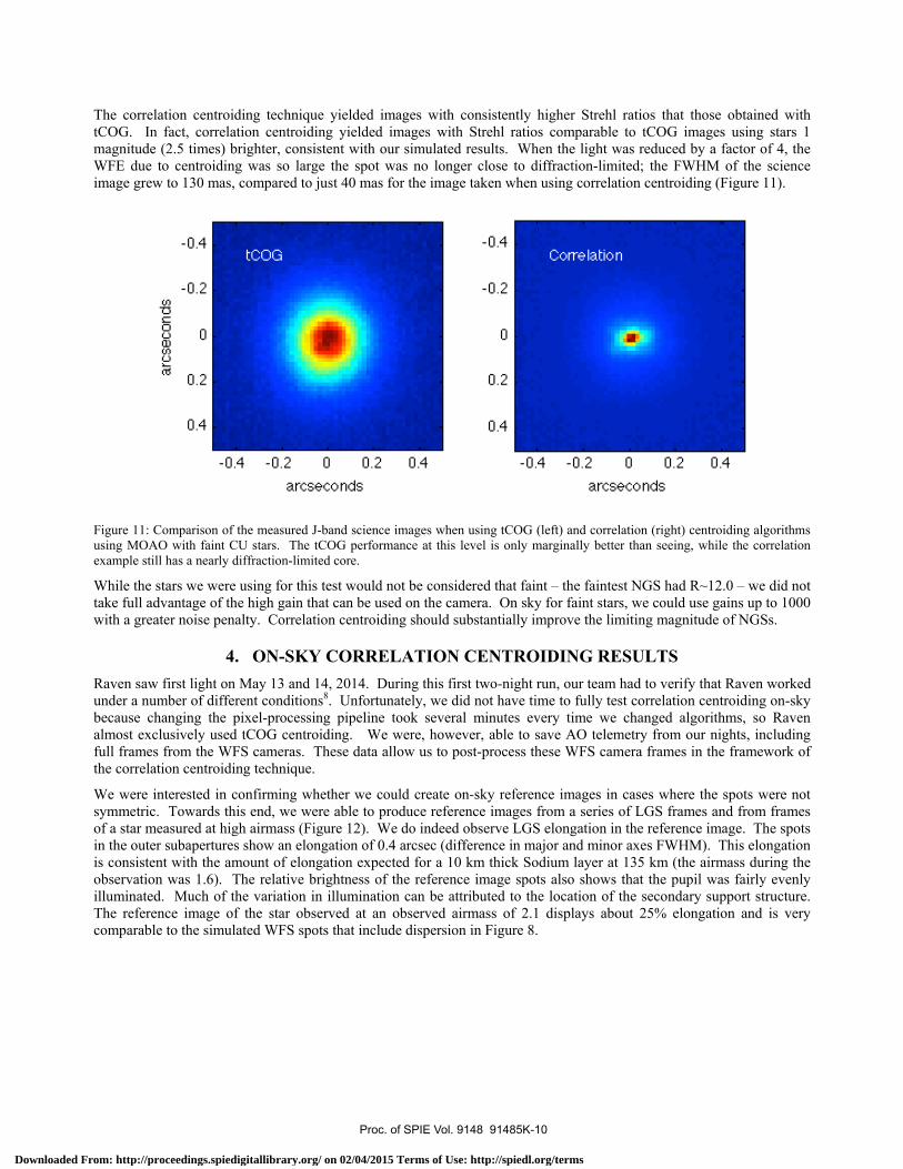
The correlation centroiding technique yielded images with consistently higher Strehl ratios that those obtained with tCOG. In fact, correlation centroiding yielded images with Strehl ratios comparable to tCOG images using stars 1 magnitude (2.5 times) brighter, consistent with our simulated results. When the light was reduced by a factor of 4, the WFE due to centroiding was so large the spot was no longer close to diffraction-limited; the FWHM of the science image grew to 130 mas, compared to just 40 mas for the image taken when using correlation centroiding (Figure 11).

Figure 11: Comparison of the measured J-band science images when using tCOG (left) and correlation (right) centroiding algorithms using MOAO with faint CU stars. The tCOG performance at this level is only marginally better than seeing, while the correlation example still has a nearly diffraction-limited core.

While the stars we were using for this test would not be considered that faint – the faintest NGS had R~12.0 – we did not take full advantage of the high gain that can be used on the camera. On sky for faint stars, we could use gains up to 1000 with a greater noise penalty. Correlation centroiding should substantially improve the limiting magnitude of NGSs.

4. ON-SKY CORRELATION CENTROIDING RESULTS Raven saw first light on May 13 and 14, 2014. During this first two-night run, our team had to verify that Raven worked under a number of different conditions8. Unfortunately, we did not have time to fully test correlation centroiding on-sky because changing the pixel-processing pipeline took several minutes every time we changed algorithms, so Raven almost exclusively used tCOG centroiding. We were, however, able to save AO telemetry from our nights, including full frames from the WFS cameras. These data allow us to post-process these WFS camera frames in the framework of the correlation centroiding technique.

We were interested in confirming whether we could create on-sky reference images in cases where the spots were not symmetric. Towards this end, we were able to produce reference images from a series of LGS frames and from frames of a star measured at high airmass (Figure 12). We do indeed observe LGS elongation in the reference image. The spots in the outer subapertures show an elongation of 0.4 arcsec (difference in major and minor axes FWHM). This elongation is consistent with the amount of elongation expected for a 10 km thick Sodium layer at 135 km (the airmass during the observation was 1.6). The relative brightness of the reference image spots also shows that the pupil was fairly evenly illuminated. Much of the variation in illumination can be attributed to the location of the secondary support structure. The reference image of the star observed at an observed airmass of 2.1 displays about 25% elongation and is very comparable to the simulated WFS spots that include dispersion in Figure 8.



..o

o I+ N 'F V'

tCO

G -

Cor

rela

tion

Rhi

S d

iffer

ence

o0

00

ó-

ivw

:;.o

t1

II

1I

I1

II

lI

TI

Ii

TI

I1

11

1

- - n- .

.1

11

1. I

I1

11

1 1

1I

1I

O CV

CV -t co co

; G.1 rI G:__;i=1;='

C*1

CO

-r

ITO

1:

D

fl

Figure 12: Left Panel: Reference images derived from on-sky Subaru LGS. The radial elongation of the reference images is consistent with a 10 km thick Sodium layer at 135 km (the airmass during the observation was 1.6). Right Panel: Reference image of NGS spot imaged at an airmass of 2.1. The reference image is comparable to the K5III star shown in Figure 8.

Finally, we wanted to assess the performance improvement we might expect when we use correlation centroiding to sense wavefronts using faint stars. During the first run, we collected time series of frames taken with WFSs observing stars of varying magnitudes from R=10.2 to R=15.1. For each set of frames, we measure the centroids using tCOG and correlation centroiding. While the standard deviation of slopes measured from each series includes signal from the turbulence and WFS noise, we expect that the quadrature difference of the RMS slopes for the two methods should be an accurate measure of the WFS noise alone. We plot this quadrature difference versus magnitude in Figure 13. We found that correlation centroiding always had a smaller standard deviation than that measured using tCOG. Furthermore, the difference increases for fainter stars. This is consistent with what we expected from simulation.

Figure 13: Quadrature difference in RMS slopes measured using the tCOG and correlation algorithms (in units of arcseconds). For brighter stars, the difference was small, but the correlation algorithm always produced slopes with a smaller RMS value. For stars fainter than R>13.5, the difference increases; correlation centroiding gives more accurate slope measurements at fainter magnitudes than tCOG.



-2

,,, -1

UL06 1

2

% C

1-2 -1 0 1

aresecondE

2

-2

-1

0

1

2

-2 -1 0 1

areseconds.

2

Figure 14: From the R=15.1 faint NGS observed with Raven, we show an example of a typical subaperture spot measured at 125 Hz and a gain of 1000. The left panel shows the spot with the measured tCOG centroid as a white circle. The right panel shows the subaperture after convolution with the reference image. The white spot shows the location of the correlation centroid.

Finally, the real WFS frames showed significant, non-Gaussian noise that was not present in the simulations. This is to be expected in real systems, but it led us to use absolute thresholds that are quite high. For fainter stars, this absolute threshold sometimes was greater that the peak value. When this occurred, no slope measurement was possible. In our measurements here, we discarded those subapertures from our measurements. The pixel-processing pipeline of Raven does not have that luxury. If no slope is returned from the tCOG (or the correlation) function, the pipeline uses a stale slope measurement from the last slope measurement where the data was greater than the threshold (if no previous valid measurement has been made the pipeline sets the centroid to the center of the subaperture). For the R=15.1 star, 0.5% of the subapertures had flux below the noise threshold we used when using tCOG centroiding which limits our ability to use tCOG for faint stars. When we switched to correlation centroiding, more peak fluxes exceeded the same absolute threshold and only 0.03% of the subapertures failed to have flux exceeding the absolute threshold. Even for a R=14.4 NGS star, we failed to record a valid slope in 0.05% of the subapertures using tCOG while correlation successfully measured slopes for virtually every subaperture.

5. CONCLUSION We have shown through simulation, lab experimentation, and analysis of on-sky data that correlation centroiding is more accurate that tCOG when open loop centroiding. While this is not a surprise, being able to implement correlation centroiding in six WFS simultaneously with only a relatively small drop in the maximum Raven frame rate (from 250 Hz to 150 Hz) showed that correlation centroiding can be used in future on-sky AO systems. Correlation centroiding is particularly powerful in open loop AO systems where a large dynamic range is required on the WFS. Reference images, built from on-sky data, can effectively recover a bit of resolution (similar to reducing the plate scale) that in turn helps reduce the aliasing error. The method is also effective at suppressing noise in the large FOV required in open loop WFSs.

We have confirmed that the combination of aliasing plus sampling error determined from MAOS simulations and included in our Raven modeling paper does not exceed 125 nm RMS. While correlation and tCOG centroiding techniques work equally well for bright stars with finely sampled WFSs, correlation centroiding works better when NGS PSFs are under-sampled and when the S/N is low. Correlation centroiding works slightly better when the reference images are created through drizzling (which increases the pixel sampling), but it is not worth up-sampling the data beyond a factor of two. Correlation centroiding can work with synthetic reference images with a small penalty in performance (2% loss in EE) if synthetic reference images are up to 50% larger than the best data-derived reference images.



For bright stars, Raven performance is not much affected by atmospheric dispersion. Raven would have worked a little better at high airmass if the WFSs had been designed to include ADCs, but for typical red NGSs, the limiting magnitude drops by less than 0.2 mag for moderate zenith angles (< 45 degrees) if correlation centroiding is used. We believe the slight drop in the limiting magnitude is not worth the extra complexity (and loss in throughput at low airmasses) if ADCs had been added.

Before the next Raven engineering nights, we will streamline the pixel processing pipeline of Raven in order to make the switch between tCOG and correlation algorithms seamless. We expect correlation centroiding will become the baseline method used for Raven by that next run. By making this switch, we believe the limiting magnitude for Raven will reach 0.5 to 1 magnitude fainter.

REFERENCES

[1] Hammer, F. et al, “The FALCON Concept: Multi-Object Spectroscopy Combined with MCAO in Near-IR,” Scientific Drivers for ESO Future VLT/VLTI Instrumentation, ed. J. Bergeron, G. Monnet, 139 (2002).

[2] Eikenberry, S. et al. “IRMOS: The near-infrared multi-object spectrograph for the TMT,” Proc. SPIE 6269, 62695E (2006).

[3] Gavel, D., Bauman, B., Dekany, R., Britton, M., Andersen, D. “Adaptive optics designs for an infrared multi-object spectrograph on TMT,” Proc. SPIE, 6272, 62720R (2006).

[4] Cuby, J-G, et al. “EAGLE: a MOAO fed multi-IFU NIR workhorse for E-ELT,” Proc. SPIE 7735, 77352D, (2010). [5] Gavel, D. et al. “Visible light laser guidestar experimental system (Villages): on-sky tests of new technologies for

visible wavelength all-sky coverage adaptive optics systems,” proc. SPIE, 7015, 8G (2008). [6] Andersen, D.R., et al. “VOLT: the Victoria Open Loop Testbed,” proc. SPIE, 7015, 9A (2008). [7] Gendron, E., et al. “MOAO first on-sky demonstration with CANARY,” A&A Letters, 529, 2 (2011). [8] Lardière, O. et al. “Multi-Object Adaptive Optics On-Sky Results with Raven,” these proceedings (2014). [9] Jackson, K. et al. “Tomography and calibration for Raven: from simulations to laboratory results,” these

proceedings (2014). [10] Tokunaga, A. et al. “Infrared camera and spectrograph for the SUBARU Telescope,” proc. SPIE, 3354, 512 (1998). [11] Andersen, D.R. et al. “Performance Modeling for the RAVEN Multi-Object Adaptive Optics Demonstrator,” PASP,

124, 469 (2012). [12] Lardière, O. et al. “Final opto-mechanical design of Raven, a MOAO science demonstrator for Subaru,” proc. SPIE,

8447, 844753 (2012). [13] Correia, C. et al. “Static and predictive tomographic reconstruction for wide-field multi-object adaptive optics

systems,” JOSA A, 31, 101 (2014). [14] Thomas, S., et al. “Comparison of centroid computation algorithms in a Shack-Hartmann sensor,” MNRAS, 371,

323 (2006). [15] Basden, A.G., et al. “Real-time correlation reference update for astronomical adaptive optics,” MNRAS, 439, 968

(2014). [16] Gilles, L., Ellerbroek, B., “Shack-Hartmann wavefront sensing with elongated sodium laser beacons: centroiding

versus matched filtering,” Applied Optics, 45, 6568, (2006). [17] Lavigne, J.-F. et al. “Design and test results of the calibration unit for the MOAO demonstrator Raven,” proc. SPIE

8447, 844754 (2012).



Documents

Comparing the performance of open loop centroiding ...web.uvic.ca/~ravenmoa/Docs/Andersen_SPIE_2014.pdf · Comparing the performance of open loop centroiding techniques in the Raven