Comparing deep neural networks against humans:object recognition when the signal gets weaker

Robert Geirhos1,2, David H. J. Janssen1,3, Heiko H. Schutt1,4,5,Jonas Rauber2,3, Matthias Bethge2,6,7, and Felix A. Wichmann1,2,6,8

1Neural Information Processing Group, University of Tubingen, Germany2Centre for Integrative Neuroscience, University of Tubingen, Germany

3Graduate School of Neural Information Processing, University of Tubingen, Germany4Graduate School of Neural and Behavioural Sciences, University of Tubingen, Germany

5Department of Psychology, University of Potsdam, Germany6Bernstein Center for Computational Neuroscience, Tubingen, Germany7Max Planck Institute for Biological Cybernetics, Tubingen, Germany

8Max Planck Institute for Intelligent Systems, Tubingen, Germany

Abstract

Human visual object recognition is typically rapid and seemingly effortless, aswell as largely independent of viewpoint and object orientation. Until very recently,animate visual systems were the only ones capable of this remarkable computationalfeat. This has changed with the rise of a class of computer vision algorithms calleddeep neural networks (DNNs) that achieve human-level classification performanceon object recognition tasks. Furthermore, a growing number of studies report sim-ilarities in the way DNNs and the human visual system process objects, suggestingthat current DNNs may be good models of human visual object recognition. Yetthere clearly exist important architectural and processing differences between state-of-the-art DNNs and the primate visual system. The potential behavioural conse-quences of these differences are not well understood. We aim to address this issueby comparing human and DNN generalisation abilities towards image degradations.We find the human visual system to be more robust to image manipulations likecontrast reduction, additive noise or novel eidolon-distortions. In addition, we findprogressively diverging classification error-patterns between man and DNNs whenthe signal gets weaker, indicating that there may still be marked differences in theway humans and current DNNs perform visual object recognition. We envisionthat our findings as well as our carefully measured and freely available behaviouraldatasets1 provide a new useful benchmark for the computer vision community toimprove the robustness of DNNs and a motivation for neuroscientists to search formechanisms in the brain that could facilitate this robustness.

1Data and materials available at https://github.com/rgeirhos/object-recognition

1

arX

iv:1

706.

0696

9v1

[cs

.CV

] 2

1 Ju

n 20

17

1 Introduction

The visual recognition of objects by humans in everyday life is typically rapid andeffortless, as well as largely independent of viewpoint and object orientation (e.g.Biederman, 1987). This ability of the primate visual system has been termed coreobject recognition, and much research has been devoted to understanding this pro-cess (see DiCarlo, Zoccolan, & Rust, 2012, for a review). We know, for example,that it is possible to reliably identify objects in the central visual field within asingle fixation in less than 200 ms when viewing “standard” images (DiCarlo etal., 2012; Potter, 1976; Thorpe, Fize, & Marlot, 1996). Based on the rapidnessof object recognition, core object recognition is often hypothesized to be achievedwith mainly feedforward processing although feedback connections are ubiquitousin the primate brain (but see, e.g. Gerstner, 2005, for a critical assessment of thisargument). Object recognition is believed to be realized by the ventral visual path-way, a hierarchical structure consisting of the areas V1-V2-V4-IT, with informationfrom the retina reaching the cortex in V1 (e.g. Goodale & Milner, 1992). Althoughaspects of this process are known, others remain unclear.

Until very recently, animate visual systems were the only known systems capableof visual object recognition. This has changed, however, with the advent of brain-inspired deep neural networks (DNNs) which, after having been trained on millionsof labeled images, achieve human-level performance when classifying objects inimages of natural scenes (Krizhevsky, Sutskever, & Hinton, 2012). DNNs are nowemployed on a variety of tasks and set the new state-of-the-art, sometimes evensurpassing human performance on tasks which were a few years ago thought to bebeyond an algorithmic solution for decades to come (He, Zhang, Ren, & Sun, 2015;Silver et al., 2016). For an excellent introduction to DNNs see e.g. LeCun, Bengio,and Hinton (2015).

Although being in the first place an engineering discipline, the field of computervision (interested in designing algorithms and building machines that can see) hasalways been interested in human vision: As in object recognition, our visual systemis often remarkably successful, acting as de facto performance benchmark for manytasks. It is thus not surprising that there has always been an exchange betweenresearchers in computer vision and human vision, such as the design of low-levelimage representations (Simoncelli, Freeman, Adelson, & Heeger, 1992; Simoncelli& Freeman, 1995) and the investigation of underlying coding principles such asredundancy reduction (Atick, 1992; Barlow, 1961; Olshausen & Field, 1996). Withthe advent of DNNs over the course of the last few years, this exchange has evendeepened. It is thus not surprising that some studies have started investigatingsimilarities between DNNs and human vision, drawing parallels between networkand biological units or network layers and visual areas in the primate brain. Clearly,describing network units as biological neurons is an enormous simplification giventhe sophisticated nature and diversity of neurons in the brain (Douglas & Martin,1991). Still, often the strength of a model lies not in replicating the original systembut rather in its ability to capture the important aspects while abstracting fromdetails of the implementation (e.g. Kriegeskorte, 2015).

2

1.1 Behavioural comparison between man and DNNs

Thorough comparisons of man and DNN behaviour have been relatively rare. Be-haviour goes well beyond overall performance: It comprises all performance changesas a function of certain stimulus properties, e.g. how classification accuracy dependson image background and contrast or the type and distribution of errors. Ideally,computational models of behaviour should not only be able to predict the over-all accuracy of humans, but be able to describe behaviour on a more fine-grainedlevel, e.g. in the current experiment on a category-by-category level. The ulti-mate goal should be the prediction of behaviour on a trial-by-trial basis, termedmolecular psychophysics (Green, 1964; Schonfelder & Wichmann, 2012). An impor-tant early step into comparing human and DNN behaviour was the work of Lake,Zaremba, Fergus, and Gureckis (2015) reporting that DNNs are able to predicthuman category typicality ratings for images. Another study by Kheradpisheh,Ghodrati, Ganjtabesh, and Masquelier (2016) found largely similar performanceon view-invariant, background-controlled object recognition and, for some DNNs,highly similar error distributions. On the other hand, so-called adversarial exam-ples have cast some doubt on the idea of broad-ranging manlike DNN behaviour.For any given image it is possible to perturb it minimally in a principled way suchthat DNNs mis-classify it as belonging to an arbitrary other category (Szegedy etal., 2014). This slightly modified image is then called an adversarial example, andthe manipulation is imperceptible to human observers (Szegedy et al., 2014).

The ease at which DNNs can be fooled speaks to the need of a careful, psy-chophysical comparison of human and DNN behaviour. As the possibility to sys-tematically search for adversarial examples is very limited in humans, it is notknown how to quantitatively compare the robustness of humans and machinesagainst adversarial attacks. However, other behavioural measurements are knownto have contributed much to our current understanding of the human visual sys-tem: Psychophysical investigations of human behaviour on object recognition tasks,measuring accuracies depending on image colour (grayscale vs. colour), image con-trast and the amount of additive visual noise have been powerful means of ex-ploring the human visual system, revealing much about the internal computationsand mechanisms at work (e.g. Nachmias & Sansbury, 1974; Pelli & Farell, 1999;Wichmann, 1999; Henning, Bird, & Wichmann, 2002; Carandini & Heeger, 2012;Carandini, Heeger, & Movshon, 1997; Delorme, Richard, & Fabre-Thorpe, 2000).As a consequence, similar experiments might yield equally interesting insights intothe functioning of DNNs, especially as a comparison to human behaviour. In thisstudy, we obtain and analyse human and DNN classification data for the threeabove-mentioned, well-known image degradations. In addition, we employ a novelimage manipulation method. The stimuli generated by the so-called eidolon-factory(Koenderink, Valsecchi, van Doorn, Wagemans, & Gegenfurtner, 2017) are para-metrically controlled distortion of an image. Eidolons aim to evoke similar visualawareness as objects perceived in the periphery, giving them some biological justi-fication. To our knowledge, we are among the first to measure DNN performanceon these tasks and compare their behaviour to carefully measured human data, inparticular using a controlled lab environment (instead of Amazon Mechanical Turkwithout sufficient control about presentation times, display calibration, viewingangles, and sustained attention of participants).

3

In this study, we employ a paradigm2 aimed at comparing human observers andDNNs as fair as possible using an image categorization task with short presentationtimes (200 ms) along with backwards masking by a high-contrast 1/f noise mask,known to minimize, as much as psychophysically possible, feedback influence in thebrain. This is important since all investigated networks rely on purely feedforwardcomputations. We perform psychophysical experiments on man and machine andassess how robust the three DNNs AlexNet (Krizhevsky et al., 2012), GoogLeNet(Szegedy et al., 2015) and VGG-16 (Simonyan & Zisserman, 2015) are towardsimage degradations.

DNNs provide exciting new opportunities for computational modelling of vision—and we envisage DNNs to have a major impact on our understanding of humanvision in the future, essentially agreeing with assessments voiced by Kriegeskorte(2015), Kietzmann, McClure, and Kriegeskorte (2017) and VanRullen (2017). Withthis study, we aim to shed light on the behavioural consequences of the currentlyexisting architectural, processing and training differences between the tested DNNsand the primate brain. We envision that our analyses as well as our carefully mea-sured and freely available behavioural datasets (https://github.com/rgeirhos/object-recognition) may provide a new useful benchmark for the computer visioncommunity to improve the robustness of DNNs and a motivation for neuroscientiststo search for mechanisms in the brain that could facilitate human robustness.

2 Methods

2.1 General

We tested four ways of degrading images: conversion to grayscale, reducing imagecontrast, adding uniform white noise, and increasing the strength of a novel imagedistortion from the eidolon toolbox (Koenderink et al., 2017). Here we give anoverview about the experimental procedure and about the observers and deep neuralnetworks that performed these experiments. In the Appendix we provide details onthe categories and image database used (Section A.1), as well as information aboutimage preprocessing (Section A.2), including plots of example stimuli at differentlevels of signal strength. In Section A.3 of the Appendix we list the specifics ofour experimental setup; for now it might be enough to know that images in thepsychophysical experiments were always displayed at the center of the screen at asize of 3× 3 degrees of visual angle.

2.2 Procedure

In each trial a fixation square was shown for 300 ms, followed by an image shown foronly 200 ms, in turn immediately followed by a full-contrast pink noise mask (1/fspectral shape) of the same size and duration. Participants had to choose one of16 entry-level categories (see Section A.1 for details on these categories) by clickingon a response screen shown for 1500 ms3. During the whole experiment, the screen

2This is the same paradigm as reported by Wichmann et al. (2017).3During practice trials the response screen was visible for another 300 ms in case an incorrect category

was selected, and along with a short low beep sound the correct category was highlighted by setting itsbackground to white.

4

background was set to a grey value of 0.454 in the [0, 1] range, corresponding to themean grayscale value of all images in the dataset (41.17 cd/m2). Figure 1 shows aschematic of a typical trial.

Prior to starting the experiment, all participants were shown the response screenand asked to name all categories to ensure that the task was fully clear. They wereinstructed to click on the category that they thought resembles the image best,and to guess if they were unsure. They were allowed to change their choice withinthe 1500 ms response interval; the last click on a category icon of the responsescreen was counted as the answer. The experiment was not self-paced, i.e. theresponse screen was always visible for 1500 ms and thus, each experimental triallasted exactly 2200 ms (300 ms + 200 ms + 200 ms + 1500 ms).

On separate days we conducted four different experiments with 1,280 trials perparticipant each (eidolon-experiment: three sessions of 1,280 trials each). In thecolour-experiment, we used two distinct conditions (colour vs. grayscale), whereasin the contrast-experiment and in the noise-experiment eight conditions were ex-plored (corresponding to eight different contrast values or noise power densities,respectively). In the eidolon-experiment, 24 distinct conditions were employed.For each experiment, we randomly chose 80 images per category from the pool ofimages without replacement (i.e., no observer ever saw an image more than oncethroughout the entire experiment). Within each category, all conditions were coun-terbalanced. Stimulus selection was done individually for each participant to reducethe probability of an accidental bias in the image selection. Images within the ex-periments were presented in randomized order. After 256 trials (colour-experiment,noise-experiment and eidolon-experiment) and 128 trials (contrast-experiment), themean performance of the last block was displayed on the screen, and observers werefree to take a short break. The total time necessary to complete all trials was 47minutes per session, not including breaks and practice trials. In total, the resultsreported in this article are based on 39,680 psychophysical trials. Ahead of eachexperiment, all observers conducted approximately 10 minutes of practice trials togain familiarity with the task and the position of the categories on the responsescreen.

2.3 Observers and deep neural networks

Three observers participated in the colour-experiment (all male; 22 to 28 years;mean: 25 years). In each of the other experiments, five observers took part(contrast-experiment and noise-experiment: one female, four male; 20 to 28 years;mean: 23 years. Eidolon-experiment: three female, two male; 19 to 28 years;mean: 22 years). Subject-01 is an author and participated in all but the eidolon-experiment. All other participants were either paid e 10 per hour for their partic-ipation or gained course credit. All observers were students of the University ofTubingen and reported normal or corrected-to-normal vision.

We used three DNNs for our analysis: AlexNet (Krizhevsky et al., 2012),GoogLeNet (Szegedy et al., 2015) and VGG-16 (Simonyan & Zisserman, 2015).All three networks were specified within the Caffe framework (Jia et al., 2014) andacquired as a pre-trained model. VGG-16 was obtained from the Visual GeometryGroup’s website (http://www.robots.ox.ac.uk/~vgg/); AlexNet and GoogLeNetfrom the BLVC model zoo website (https://github.com/BVLC/caffe/wiki/Model-Zoo). We reproduced the respective specified accuracies on the ILSVRC 2012 val-

5

300ms

200ms

200ms

Figure 1. Schematic of a trial. After the presentation of a central fixation square(300 ms), the image was visible for 200 ms, followed immediately by a noise-maskwith 1/f spectrum (200 ms). Then, a response screen appeared for 1500 ms, duringwhich the observer clicked on a category. Note that we increased the contrast ofthe noise-mask in this figure for better visibility when printed. Categories row-wisefrom top to bottom: knife, bicycle, bear, truck, airplane, clock, boat,

car, keyboard, oven, cat, bird, elephant, chair, bottle, dog. The iconsare a modified version of the ones from the MS COCO website (http://mscoco.org/explore/).

idation dataset in our setting.All DNNs require images to be specified using RGB planes; to evaluate the

performance using grayscale images we stacked a grayscale image three times inorder to obtain the desired form specified by the caffe.io module (https://github.com/BVLC/caffe/blob/master/python/caffe/io.py). Images were fed throughthe networks using a single feedforward pass of the 224× 224 pixels center crop.

3 Results

Trials in which human observers failed to click on any category were recorded asan incorrect answer in the data analysis, and are shown as a separate category (toprow) in the confusion matrices (DNNs, obviously, never fail to respond). Such afailure to respond occurred in only 1.2% of all trials, and did not differ meaningfullybetween the different experiments. The terms ’accuracy’ and ’performance’ are usedinterchangeably. All data, if not stated otherwise, were analyzed using R version3.2.3 (R Core Team, 2016).

3.1 Accuracy and response distribution entropy

When showing accuracy in any of the plots, the error bars provided have two distinctmeanings: First, for DNNs they indicate the range of DNN accuracies resulting from

6

seven4 runs on different images, with each run consisting of the same number ofimages per category and condition that a single human observer was exposed to.This serves as an estimate of the variability of DNN accuracies as a function of therandom choice of images. Second, the error bars for human participants likewisecorrespond to the range of their accuracies (not the often shown S.E. of the means,which would be much smaller).

In addition we assessed the response distribution entropy of DNNs and man as afunction of image degradation strength. Entropy is a measure quantifying how closea distribution is to the uniform distribution (the higher the entropy, the closer it is).The distribution obtained by throwing a fair die many times should therefore havehigher entropy than the distribution obtained from repeatedly throwing a riggeddie. In the context of our experiments, it is used to measure whether observersor DNNs exhibit a bias towards certain categories: if so, the response distributionentropy will be lower than the maximal value of 4 bits (given 16 categories). Wecalculated the Shannon entropy H of response distribution X as follows:H(X ) = −

∑16i=1 p(xi)log2(p(xi)), with p(xi) being the fraction of responses for

category i (e.g. p(xcar) = 0.25 if an observer responds car every fourth trial onaverage).

3.1.1 Colour-experiment

We conducted a paired-samples t-test to assess the difference in accuracy betweencoloured and grayscale images for each network and observer (Table 2 in the Ap-pendix). In order to account for multiple comparisons, the critical significance levelof .05 was adjusted to .05

6 = .0083 by applying Bonferroni correction. As shown inFigure 2(a) all three networks performed significantly worse for grayscale imagescompared to coloured images (4.81% drop in performance on average: significant,but not dramatic in terms of effect size). Human observers, on the other hand, didnot show on average a significant reduction in accuracy (only 1.88% accuracy dropfor grayscale images). As can be seen from the range of human grayscale results,obsververs differed in their ability to cope with grayscale images.

The response distribution entropy shown in Figure 2(b) is innocuous: The DNNsdistributed their responses perfectly among the 16 categories, and human observersare only marginally worse.

3.1.2 Contrast-experiment

As shown in Figure 3(a), accuracies for the contrast-experiment ranged from ap-proximately 91−94% (VGG-16, GoogLeNet and human average) and 84% (AlexNet)for full contrast to chance level ( 1

16 = 6.25%) for 1% of contrast, except for VGG-16which still achieves 17.5% correct responses. AlexNet’s and GoogLeNet’s perfor-mance dropped more rapidly than human and VGG-16’s performance for lowercontrast levels.

The response distribution entropy shown in Figure 3(b) reveals, however, thatall three DNNs showed an increasing bias towards few categories (in other words,they did no longer distribute their responses evenly among the 16 categories if the

4Seven runs are the maximum possible number of runs without ever showing an image to a DNNmore than once per experiment.

7

0.80

0.85

0.90

0.95

1.00

Cla

ssifi

catio

n ac

cura

cy

Color Grayscale

●

●

(a) Colour-experiment accuracy

3.5

3.6

3.7

3.8

3.9

4.0

Ent

ropy

of r

espo

nse

dist

ribut

ion

[bits

]

Color Grayscale

●●

●

AlexNetGoogLeNetVGG−16participants (avg.)

(b) Colour-experiment entropy

Figure 2. Results for the colour-experiment (n=3). (a) Accuracy. DNNs are shownin shades of blue, human data in red; diamonds correspond to AlexNet, squaresto GoogLeNet, triangles to VGG-16, and circles to human observers; error bars asdescribed in section 3.1. (b) Response distribution entropy. Plotting conventions asin (a).

contrast was lowered). Human observers, on the other hand, still largely distributedtheir responses sensibly across the 16 categories.

3.1.3 Noise-experiment

The data for the noise-experiment were analyzed in the same way as the contrast-experiment data. Overall, we found drastic differences in classification accuracy,with human observers clearly outperforming all three networks. As can be seenin Figure 3(c), by increasing the noise width from 0.0 (no noise) to 0.1, VGG-16’sperformance drops from an accuracy of 89.91% to 44.02%; GoogLeNet’s drops from81.70% to 34.02% and AlexNet’s from 70.00% to 19.29%. Human observers, on theother hand, only drop from 80.50% to 75.13%.

The response distribution entropy shown in Figure 3(d) shows again that all ofthe investigated DNNs exhibit a strong bias towards few categories if the imagescontained additive noise. For AlexNet and GoogLeNet, the response distributionentropy is close to 0 bits for a noise width of 0.6 or more, which means that theyresponded with a single category for these images (category bottle for both).Interestingly, these preferred categories are usually not the same across experimentsor networks (Figures 6 and 9), and they do not simply match the probabilities ofthe categories in the ImageNet training database. The network responses thereforeare not converging to their prior distribution, which would be a sensible way tobehave in the absence of a signal. Human observers, as with low contrast, largelydistributed their responses evenly across the 16 categories.

8

2.0 1.5 1.0 0.5 0.0

0.0

0.2

0.4

0.6

0.8

1.0

Log10 of contrast in percent

Cla

ssifi

catio

n ac

cura

cy

●

●

●

●●

●●●

●

AlexNetGoogLeNetVGG−16participants (avg.)

(a) Contrast-experiment accuracy

2.0 1.5 1.0 0.5 0.0

01

23

4

Log10 of contrast in percent

Ent

ropy

of r

espo

nse

dist

ribut

ion

[bits

]

●

●●

●●●●●

(b) Contrast-experiment entropy

0.0 0.2 0.4 0.6 0.8 1.0

0.0

0.2

0.4

0.6

0.8

1.0

[−w, w] is the range of additive uniform noisew

Cla

ssifi

catio

n ac

cura

cy

●●●●

●

●

●

●

●

AlexNetGoogLeNetVGG−16participants (avg.)

(c) Noise-experiment accuracy

0.0 0.2 0.4 0.6 0.8 1.0

01

23

4

[−w, w] is the range of additive uniform noisew

Ent

ropy

of r

espo

nse

dist

ribut

ion

[bits

]

●●● ● ● ●● ●

(d) Noise-experiment entropy

0 1 2 3 4 5 6 7

0.0

0.2

0.4

0.6

0.8

1.0

Log2 of reach

Cla

ssifi

catio

n ac

cura

cy

● ●●

●

●

●

●●

●

AlexNetGoogLeNetVGG−16participants (avg.)

(e) Eidolon-experiment accuracy (co-herence parameter = 1.0)

0 1 2 3 4 5 6 7

01

23

4

Log2 of reach

Ent

ropy

of r

espo

nse

dist

ribut

ion

[bits

]

● ● ● ● ●●

● ●

(f) Eidolon-experiment entropy

Figure 3. Results for contrast-, noise- and eidolon-experiment (n=5 each).(a, c, e)(Left) Accuracy. Plotting conventions as in Figure 2.(b, d, f)(Right) Response distribution entropy.

9

3.1.4 Eidolon-experiment

Results for the eidolon-experiment with maximal coherence of 1.0 are shown in Fig-ure 3(e) and (f). The complete results of the eidolon-experiment for all coherencesettings are provided in the Appendix, Figure 11. In terms of accuracy, networkand human performance naturally were approximately equal for very low values ofreach (no distortion, therefore high accuracies) and for very high values of reach(heavy distortion, accuracy at chance level). In the range between these extremes,their accuracies followed the typically observed s-shaped pattern known from mostpsychophysical experiments varying a single parameter. However, human observersclearly achieved higher accuracies than all three networks for intermediate distor-tions. In the full coherence case, the largest difference between network and humanperformance was observed for a reach value of 23 = 8 (38.3% network accuracy vs.75.3% human accuracy, averaged across networks and observers). The coherence-parameter, albeit having a considerable effect on the perceptual appearance of thestimuli, did not qualitatively change accuracies. Quantitatively, the performancewas generally higher for high coherence values (see Figure 11 for details). Unlike inthe case of contrast, the three networks showed only minor inter-network accuracydifferences.

As for the contrast-experiment and the noise-experiment, we find all three net-works to be strongly biased towards a few categories as shown by their low responsedistribution entropy (Figure 3f).

3.1.5 Performance visualization

Here we provide a visualization of the performance differences between the studiedDNNs and human observers in terms of their generalisation ability (or robustnessagainst image degradations). For all degradation-types—contrast, noise, eidolonswith different coherence parameters—we estimated the stimulus levels correspond-ing to 50% classification accuracy. The stimulus levels were calculated assuming alinear relationship between the two closest data points measured in the experimentsand shown in the left column of Figure 3.

Figure 4(a) shows the 50% accuracies for the noise-experiment, Figure 4(b) forthe eidolon-experiment with maximal coherence (as in Figures 3(e) and (f)); thethree illustration images of categories bicycle, dog and keyboard were drawn ran-domly from the pool of images used in the experiments. In both panels the top rowshows the stimuli corresponding to 50% accuracy for the average human observer.The bottom three rows show the corresponding stimuli for VGG-16 (second row),GoogLeNet (third row) and AlexNet (bottom row). On a typical computer screenthe more robust performance of human observers over DNNs should be readily ap-preciable. 50% accuracy stimulus plots for the contrast-experiment and the otherconditions of the eidolon-experiment can be found in the Appendix, Figure 12.

3.2 Confusion and confusion difference matrices

Confusion matrices are a widely used tool for visualizing error patterns in multi-class classification data, providing insight into classification behavior (e.g.: doesVGG-16 frequently confuse dogs with cats?). Figure 5(a) shows a standard con-fusion matrix of the colour condition in the colour-experiment (Section 3.1.1) for

10

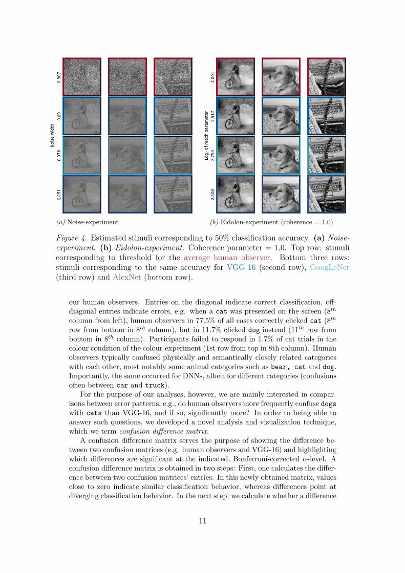
(a) Noise-experiment (b) Eidolon-experiment (coherence = 1.0)

Figure 4. Estimated stimuli corresponding to 50% classification accuracy. (a) Noise-experiment. (b) Eidolon-experiment. Coherence parameter = 1.0. Top row: stimulicorresponding to threshold for the average human observer. Bottom three rows:stimuli corresponding to the same accuracy for VGG-16 (second row), GoogLeNet(third row) and AlexNet (bottom row).

our human observers. Entries on the diagonal indicate correct classification, off-diagonal entries indicate errors, e.g. when a cat was presented on the screen (8th

column from left), human observers in 77.5% of all cases correctly clicked cat (8th

row from bottom in 8th column), but in 11.7% clicked dog instead (11th row frombottom in 8th column). Participants failed to respond in 1.7% of cat trials in thecolour condition of the colour-experiment (1st row from top in 8th column). Humanobservers typically confused physically and semantically closely related categorieswith each other, most notably some animal categories such as bear, cat and dog.Importantly, the same occurred for DNNs, albeit for different categories (confusionsoften between car and truck).

For the purpose of our analyses, however, we are mainly interested in compar-isons between error patterns, e.g., do human observers more frequently confuse dogswith cats than VGG-16, and if so, significantly more? In order to being able toanswer such questions, we developed a novel analysis and visualization technique,which we term confusion difference matrix.

A confusion difference matrix serves the purpose of showing the difference be-tween two confusion matrices (e.g. human observers and VGG-16) and highlightingwhich differences are significant at the indicated, Bonferroni-corrected α-level. Aconfusion difference matrix is obtained in two steps: First, one calculates the differ-ence between two confusion matrices’ entries. In this newly obtained matrix, valuesclose to zero indicate similar classification behavior, whereas differences point atdiverging classification behavior. In the next step, we calculate whether a difference

11

(a) Colour-experiment, colour-condition, humanparticipants.

(b) Colour-experiment, colour-condition, differ-ence between human participants and VGG-16.

Figure 5. Confusion and confusion difference matrices for colour-experiment (colour-condition only). A failure to respond is shown as a separate category in the toprow here. (a) Standard confusion matrix. Entries on the diagonal indicate correctclassification, off-diagonal entries indicate errors. (b) Confusion difference matrix.All values indicate the signed difference of human observers’ and VGG-16’s confu-sion matrix entries. A positive sign indicates that human observers responded morefrequently than VGG-16 to a certain category-response pair, for a negative sign vice-versa. The colour here indicates whether a difference for a certain cell is significantat α = 5%

16·17(∗), 1%16·17(∗∗) and 0.1%

16·17(∗ ∗ ∗); these α-levels are Bonferroni corrected formultiple comparisons (16 categories · 17 possible responses); see text in Section 3.2for details.

12

for a certain cell is significant, and repeat this calculation for all cells. We calculatesignificance using a standard test of the probability of success in a Binomial exper-iment: If one thinks of the 120 colour-experiment trials in which human observerswere exposed to a coloured cat image, of which they clicked on cat in 93 trials,as of a Binomial experiment with 93 successes out of 120 trials, is “93 out of 120”significantly higher or lower than we would expect under the null hypothesis ofsuccess probability p = 96.8% (VGG-16’s fraction of responses in this cell5)? TheBinomial tests were performed with R, using the binom.test function of packagestats which calculates the conservative Clopper-Pearson confidence interval6. Thesignificance of a certain difference, in our experiments, is not used for traditionalhypothesis testing but rather as a means of distinguishing between important andunimportant—perhaps only coincidental—behavioural differences between man andDNNs even if their accuracies were equal. Confusion difference matrices thus vi-sualize systematic category-dependent error pattern differences between man andDNNs—and they do this at a much more fine-grained, category-specific level thanthe response distribution entropy analyses shown in Section 3.1.

Figure 5(b) shows one confusion difference matrix for the colour-experiment(colour-condition only); all values indicate the signed difference of human observers’and VGG-16’s confusion matrix entries. A positive sign indicates that human ob-servers responded more frequently than VGG-16 to a certain category-responsepair, for a negative sign vice-versa. VGG-16 is significantly better for many cate-gories on the diagonal (correct classification) because—in the non-degraded colourcondition—human observers make more errors, see Figure 2(a). Overall, however,most cells of the confusion difference matrix are grey, indicating very similar clas-sification behaviour of man and VGG-16, not only in terms of overall accuracy andresponse entropy, but on a fine-grained category-by-category level.

In Figure 6 we show a confusion difference matrix grid for the noise-experiment(Section 3.1.3): nine confusion difference matrices for all three DNNs at threematched performance levels. Confusion difference matrices shown here are calcu-lated as described above, however, with the important difference that we here showdifference matrices for which human observers and networks have similar overallperformance (accuracy difference < 5%): we compare confusion matrices for dif-ferent stimulus levels, but matched in performance7. The left column shows highperformance (no noise for human observers, very little noise for DNNs; performancep-high = 80.5% which corresponds, in this order, to w = 0.0, 0.0, 0.0 and 0.03 forhuman observers, AlexNet, GoogLeNet and VGG-16). On the right, data for lowperformance (16.8%) are shown (high noise for human observers, moderate-to-lownoise for DNNs, w = 0.60, 0.10, 0.15, 0.19) and in the middle results for mediumperformance: 45.6%, the condition for which human observers’ accuracy was ap-proximately equal to 1

2(p-high + p-low) (medium noise for human observers, low

5It would also be possible compare VGG-16’s number of successes to human observers’ fraction ofresponses. We always compared the network/observer/group with less trials to the one with more trialsas null hypothesis—in the example above (colour-experiment, colour-condition, cat images): a total of120 trials for human observers vs. 280 trials for VGG-16 (or any other network).

6If the network’s fraction of responses in a certain cell was 0.0% (not a single response in this cell),we set p = 0.1% and if it was 100.0% (every time a certain category was presented, the response lied inthis cell), we set p = 99.9% instead.

7If DNN-human accuracy deviance was more than 5% for all conditions, we ran additional experimentsto determine a suitable condition.

13

noise for DNNs; w = 0.35, 0.06, 0.08, 0.10).Showing confusion difference matrices at matched performance levels—rather

than at the same stimulus level—has the advantage that the sum over all entriesof the to-be-compared confusion matrices is the same, i.e. for equally behavingclassifiers the expectation is to obtain mainly grey (non-significant) cells. However,inspection of Figure 6 shows this only to be the case for the easy, low-noise, condition(left column). With increasing task difficulty (more noise), network and humanbehavior diverges substantially. As the noise level increases, all networks show arapidly increasing bias for a few categories. For a noise level of w = 0.35, AlexNetand GoogLeNet almost exclusively respond bottle (92.32% and 85.71%), whereasVGG-16 homes in on category dog for 62.50% of all images. Note that this biasfor certain categories is neither consistent across networks nor across the imagemanipulations.

A similar pattern emerged for the contrast-experiment: Classification behavioron a stimulus-by-stimulus basis for all three DNNs is close to that of human ob-servers for a high accuracy (nominal contrast level). However, as task difficultyincreases, the classification behavior of all three DNNs differs significantly fromhuman behavior, despite being matched in overall accuracy (see the Appendix,Figure 9).

4 Discussion

We psychophysically examined to what extend currently well-known DNNs (AlexNet,GoogLeNet and VGG-16) could be a good model for human feedforward visual ob-ject recognition. So far thorough comparisons of DNNs and human observers onbehavioural grounds have been rare. Here we proposed a fair and psychophysicallyaccurate way of comparing network and human performance on a number of ob-ject recognition tasks: measuring categorization accuracy for single-fixation, brieflypresented (200 ms) and backward-masked images as a function of colour, contrast,uniform noise, and eidolon-type distortions.

We find that DNNs outperform human observers by a significant margin fornon-distorted, coloured images—the images the DNNs were specifically trained on.We speculate that this may in part be due to some images in the ImageNet databasecontaining images with small animals in the background, making it tough to decidewhether it is a cat, dog or even a bear. Given that the images were labelled byhuman observers—who thus are the ultimate guardians of what counts as rightor wrong—it is clear that for unlimited inspection time and sufficient training hu-man observers will equal DNN performance, as shown by the benchmark results ofRussakovsky et al. (2015), obtained using expert annotators. What we established,however, is that under conditions minimizing feedback, current DNNs already out-perform human observers on the type of images found on ImageNet..

Our first experiment also shows that human observers’ accuracy suffers onlymarginally when images are converted to grayscale in comparison to coloured im-ages, consistent with previous studies (Delorme et al., 2000; Kubilius, Bracci, &Op de Beeck, 2016; Wichmann, Braun, & Gegenfurtner, 2006)8. For all three tested

8Consistent, also, with the popularity of black-and-white movies and photography: If we had a hardtime recognizing objects and scenes in black-and-white we doubt that they’d ever have been a massmedium in the early and mid 20th century.

14

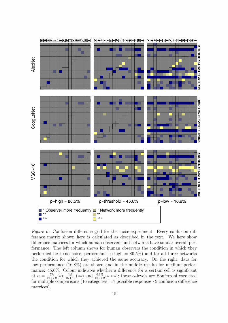
Figure 6. Confusion difference grid for the noise-experiment. Every confusion dif-ference matrix shown here is calculated as described in the text. We here showdifference matrices for which human observers and networks have similar overall per-formance. The left column shows for human observers the condition in which theyperformed best (no noise, performance p-high = 80.5%) and for all three networksthe condition for which they achieved the same accuracy. On the right, data forlow performance (16.8%) are shown and in the middle results for medium perfor-mance: 45.6%. Colour indicates whether a difference for a certain cell is significantat α = 5%

16·17·9(∗), 1%16·17·9(∗∗) and 0.1%

16·17·9(∗ ∗ ∗); these α-levels are Bonferroni correctedfor multiple comparisons (16 categories · 17 possible responses · 9 confusion differencematrices).

15

DNNs the performance decrement is significant, however. Particularly AlexNetshows a largish drop in performance (> 7%), which is not human-like. VGG-16and GoogLeNet rely less on colour information, but still somewhat more than theaverage human observer.

Our second experiment examined accuracy as a function of image contrast. Hu-man participants outperform AlexNet and GoogLeNet (but not VGG-16) in thelow contrast regime, where all DNNs display an increasing bias for certain cate-gories (Figure 3(b) as well as Figure 9). Almost all images on which the networkswere originally trained with had full contrast. Apparently, training on ImageNet initself only leads to a suboptimal contrast invariance. There are several solutions toovercome this deficiency: One option would be to include an explicit image prepro-cessing stage or have the first layer of the networks normalise the contrast. Anotheroption would be to augment the training data with images of various contrast levels,which in itself might be a worthwhile data augmentation technique even if one doesnot expect low contrast images at test time. In the human visual system, proba-bly as a response to the requirement of increasing stimulus identification accuracy(Geisler & Albrecht, 1995), a mechanism called contrast gain control evolved, serv-ing the human visual system as a contrast normalization technique by taking intoaccount the average local contrast rather than the absolute, global contrast (e.g.Carandini et al., 1997; Heeger, 1992; Sinz & Bethge, 2009, 2013). This has the(side-) effect that human observers can easily perform object recognition across avariety of contrast levels. Thus yet another, though clearly more labour-intensiveway of improving contrast invariance in DNNs would be to incorporate a mech-anism of contrast gain control directly in the network architecture. Early visionmodels could serve as a role model (e.g., Goris, Putzeys, Wagemans, & Wichmann,2013; Schutt & Wichmann, 2017).

Our third experiment, adding uniform white noise to images, shows very cleardiscrepancies between the performance of DNNs and human observers. Note that,if anything, we might have underestimated human performance: randomly shufflingall conditions of an experiment instead of using blocks of a certain stimulus level arelikely to yield accuracies that are lower than those possible in a blocked constantstimulus setting (Blackwell, 1953; Jakel & Wichmann, 2006). Already at a moderatenoise level, however, network accuracies drop sharply, whereas human observers areonly slightly affected (visualized in Figure 4 showing stimuli corresponding to 50%accuracy for human observers and the three networks). Consistent with recentresults by Dodge and Karam (2017), our data clearly show that the human visualsystem is currently much more robust to noise than any of the investigated DNNs.

Another noteworthy finding is that the three DNNs exhibit considerable inter-model differences; their ability to cope with grayscale and different levels of contrastand noise differs substantially. In combination with other studies finding moderateto striking differences (e.g. Cadieu et al., 2014; Kheradpisheh et al., 2016; Lakeet al., 2015), this speaks to the need of carefully distinguishing between modelsrather than treating DNNs as a single model type as it is perhaps sometimes donein vision science.

Recent studies on so-called adversarial examples in DNNs have demonstratedthat, for a given image, it is possible to construct a minimally perturbed versionof this image which DNNs will misclassify as belonging to an arbitrary differentcategory (Szegedy et al., 2014). Here we show that comparatively large but purelyrandom distortions such as additive uniform noise also lead to poor network per-

16

formance. Our detailed analyses of the network decisions offer some clues on whatcould contribute to robustness against these distortions, as the measurement ofconfusion matrices for different signal-to-noise ratios is a powerful tool to revealimportant algorithmic differences of visual decision making in humans and DNNs.All three DNNs show an escalating bias towards few categories as noise power den-sity increases (Figures 3 and 6), indicating that there might be something inherentto noisy images that causes the networks to select a single category. The networksmight perceive the noise as being part of the object and its texture while humanobservers perceive the noise like a layer in front of the image (you may judge thisyourself by looking at the stimuli in Figure 7). This might be the achievement of amechanism for depth-layering of surface representations implemented by mid-levelvision, which is thought to help the human brain to encode spatial relations and toorder surfaces in space (Kubilius, Wagemans, & Op de Beeck, 2014). Incorporatingsuch a depth-layering mechanism may lead to an improvement of current DNNs,enabling them to robustly classify objects even when they are distorted in a waythat the network was not exposed to during training.

It remains subject to future investigations to determine whether such a mecha-nism will emerge from augmenting the training regime with different kinds of noise,or whether changes in the network architecture, potentially inspired by knowledgeabout mid-level vision, are necessary to achieve this feat.

One might argue that human observers, through experience and evolution, wereexposed to some image distortions (e.g. fog or snow) and therefore have an advan-tage over current DNNs. However, an extensive exposure to eidolon-type distortionsseems exceedingly unlikely. And yet, human observers were considerably better atrecognising eidolon-distorted objects, largely unaffected by the different perceptualappearance for different eidolon parameter combinations (reach, coherence). Thisindicates that the representations learned by the human visual system go beyondbeing trained on certain distortions as they generalise towards previously unseendistortions. We believe that achieving such robust representations that generalisetowards novel distortions are the key to achieve robust deep neural network perfor-mance, as the number of possible distortions is literally unlimited.

4.1 Conclusion

We conducted a behavioural, psychophysical comparison of man and machine objectrecognition robustness against image degradations. While it has long been noticedthat DNNs are extremely fragile against adversarial attacks, our results show thatthey are also more prone to random perturbations than humans. In comparisonto human observers, we find the classification performance of three currently well-known DNNs trained on ImageNet—AlexNet, GoogLeNet and VGG-16—to declinerapidly with decreasing signal-to-noise ratio under image degradations like addi-tive noise or eidolon-type distortions. Additionally, by measuring and comparingconfusion matrices we find progressively diverging patterns of classification errorsbetween humans and DNNs with weaker signals, and considerable inter-model dif-ferences. Our results demonstrate that there are still marked differences in theway humans and current DNNs process object information. We envision that ourfindings and the freely available behavioural datasets may provide a new usefulbenchmark for improving DNN robustness and a motivation for neuroscientists tosearch for mechanisms in the brain that could facilitate this robustness.

17

Author contributions

R.G., H.H.S. and F.A.W. designed the study; R.G. performed the network exper-iments with input from D.H.J.J. and H.H.S.; R.G. acquired the behavioural datawith input from F.A.W.; R.G., H.H.S., J.R. M.B. and F.A.W. analysed and in-terpreted the data. R.G. and F.A.W. wrote the paper with significant input fromH.H.S., J.R., and M.B.

Acknowledgement

This work has been funded, in part, by the German Federal Ministry of Educa-tion and Research (BMBF) through the Bernstein Computational NeuroscienceProgram Tubingen (FKZ: 01GQ1002) as well as the German Research Foundation(DFG; Sachbeihilfe Wi 2103/4-1 and SFB 1233 on “Robust Vision”). M.B. acknowl-edges support by the Centre for Integrative Neuroscience Tubingen (EXC 307) andby the Intelligence Advanced Research Projects Activity (IARPA) via Departmentof Interior/Interior Business Center (DoI/IBC) contract number D16PC00003. J.R.is funded by the BOSCH Forschungsstiftung. We would like to thank Tom Wallisfor providing the MATLAB source code of one of his experiments, and for allowingus to use and modify it; Silke Gramer for administrative and Uli Wannek for tech-nical support, as well as Britta Lewke for the method of creating response iconsand Patricia Rubisch for help with testing human observers.

References

Atick, J. J. (1992). Could information theory provide an ecological theory of sensoryprocessing? Network: Computation in neural systems, 3 (2), 213–251.

Barlow, H. B. (1961). Possible principles underlying the transformations of sensory mes-sages. Sensory Communication, 217–234.

Biederman, I. (1987). Recognition-by-components: a theory of human image understand-ing. Psychological Review , 94 (2), 115-147.

Blackwell, H. R. (1953). Psychophysical thresholds: experimental studies of methods ofmeasurement. University of Michigan Engineering Research Institute Bulletin, No.36 , xiii-227.

Brainard, D. H. (1997). The psychophysics toolbox. Spatial Vision, 10 , 433–436.Cadieu, C. F., Hong, H., Yamins, D. L. K., Pinto, N., Ardila, D., Solomon, E. A., . . .

DiCarlo, J. J. (2014). Deep neural networks rival the representation of primate ITcortex for core visual object recognition. PLoS Computational Biology , 10 (12).

Carandini, M., & Heeger, D. J. (2012). Normalization as a canonical neural computation.Nature Reviews Neuroscience, 13 (1), 51–62.

Carandini, M., Heeger, D. J., & Movshon, J. A. (1997). Linearity and normalization insimple cells of the macaque primary visual cortex. The Journal of Neuroscience,17 (21), 8621–8644.

Delorme, A., Richard, G., & Fabre-Thorpe, M. (2000). Ultra-rapid categorisation ofnatural scenes does not rely on colour cues: a study in monkeys and humans. VisionResearch, 40 (16), 2187–2200.

DiCarlo, J. J., Zoccolan, D., & Rust, N. C. (2012). How does the brain solve visual objectrecognition? Neuron, 73 (3), 415–434.

Dodge, S., & Karam, L. (2017). A study and comparison of human and deep learningrecognition performance under visual distortions. arXiv preprint arXiv:1705.02498.

18

Douglas, R. J., & Martin, K. A. C. (1991). Opening the grey box. Trends in Neurosciences,14 (7), 286-293.

Geisler, W. S., & Albrecht, D. G. (1995). Bayesian analysis of identification performancein monkey visual cortex: nonlinear mechanisms and stimulus certainty. Vision Re-search, 35 (19), 2723-2730.

Gerstner, W. (2005). How can the brain be so fast? In J. L. van Hemmen & T. J. Sejnowski(Eds.), 23 problems in systems neuroscience (p. 135-142). Oxford University Press.

Goodale, M. A., & Milner, A. D. (1992). Separate visual pathways for perception andaction. Trends in Neurosciences, 15 (1), 20–25.

Goris, R. L., Putzeys, T., Wagemans, J., & Wichmann, F. A. (2013). A neural populationmodel for visual pattern detection. Psychological Review , 120 (3), 472.

Green, D. M. (1964). Consistency of auditory judgements. Psychological Review , 71 (5),592-407.

He, K., Zhang, X., Ren, S., & Sun, J. (2015). Delving deep into rectifiers: Surpassinghuman-level performance on ImageNet classification. In Proceedings of the IEEEInternational Conference on Computer Vision (pp. 1026–1034).

Heeger, D. J. (1992). Normalization of cell responses in cat striate cortex. Visual Neuro-science, 9 , 181-197.

Henning, G. B., Bird, C. M., & Wichmann, F. A. (2002). Contrast discrimination with pulsetrains in pink noise. Journal of the Optical Society of America A, 19 (7), 1259-1266.

Jakel, F., & Wichmann, F. A. (2006). Spatial four-alternative forced-choice method isthe preferred psychophysical method for naıve observers. Journal of Vision, 6 (11),1307-1322.

Jia, Y., Shelhamer, E., Donahue, J., Karayev, S., Long, J., Girshick, R., . . . Darrell, T.(2014). Caffe: Convolutional architecture for fast feature embedding. In Proceedingsof the 22nd ACM International Conference on Multimedia (pp. 675–678).

Kheradpisheh, S. R., Ghodrati, M., Ganjtabesh, M., & Masquelier, T. (2016). Deepnetworks resemble human feed-forward vision in invariant object recognition. arXivpreprint arXiv:1508.03929.

Kietzmann, T. C., McClure, P., & Kriegeskorte, N. (2017). Deep neural networks incomputational neuroscience. bioRxiv , http://dx.doi.org/10.1101/133504 .

Kleiner, M., Brainard, D., Pelli, D., Ingling, A., Murray, R., & Broussard, C. (2007).What’s new in Psychtoolbox-3. Perception, 36 (14), 1.

Koenderink, J., Valsecchi, M., van Doorn, A., Wagemans, J., & Gegenfurtner, K. (2017).Eidolons: Novel stimuli for vision research. Journal of Vision, 17 (2), 7–7.

Kriegeskorte, N. (2015). Deep neural networks: A new framework for modeling biologicalvision and brain information processing. Annual Review of Vision Science, 1 (15),417–446.

Krizhevsky, A., Sutskever, I., & Hinton, G. E. (2012). ImageNet classification with deepconvolutional neural networks. In Advances in Neural Information Processing Sys-tems (pp. 1097–1105).

Kubilius, J., Bracci, S., & Op de Beeck, H. P. (2016). Deep neural networks as a com-putational model for human shape sensitivity. PLoS Computational Biology , 12 (4),e1004896.

Kubilius, J., Wagemans, J., & Op de Beeck, H. P. (2014). A conceptual framework ofcomputations in mid-level vision. Frontiers in Computational Neuroscience, 8 , 158.

Lake, B. M., Zaremba, W., Fergus, R., & Gureckis, T. M. (2015). Deep Neural Networkspredict category typicality ratings for images. In Proceedings of the 37th AnnualConference of the Cognitive Science Society.

LeCun, Y., Bengio, Y., & Hinton, G. (2015). Deep learning. Nature, 521 (7553), 436–444.Lin, T.-Y., Maire, M., Belongie, S., Hays, J., Perona, P., Ramanan, D., . . . Zitnick, C. L.

(2015). Microsoft COCO: Common objects in context. In European Conference onComputer Vision (pp. 740–755).

Nachmias, J., & Sansbury, R. V. (1974). Grating contrast: Discrimination may be betterthan detection. Vision Research, 14 (10), 1039-1042.

19

Olshausen, B. A., & Field, D. J. (1996). Emergence of simple-cell receptive field propertiesby learning a sparse code for natural images. Nature, 381 (6583), 607.

Pelli, D. G., & Farell, B. (1999). Why use noise? Journal of the Optical Society of AmericaA, 16 (3), 647-653.

Potter, M. C. (1976). Short-term conceptual memory for pictures. Journal of ExperimentalPsychology: human learning and memory , 2 (5), 509.

R Core Team. (2016). R: A language and environment for statistical computing [Computersoftware manual]. Vienna, Austria. Retrieved from https://www.R-project.org/

Rosch, E. (1999). Principles of categorization. In E. Margolis & S. Laurence (Eds.),Concepts: core readings (pp. 189–206).

Russakovsky, O., Deng, J., Su, H., Krause, J., Satheesh, S., Ma, S., . . . Fei-Fei, L. (2015).ImageNet Large Scale Visual Recognition Challenge. International Journal of Com-puter Vision, 115 (3), 211–252.

Schutt, H. H., & Wichmann, F. A. (2017). An image-computable psychophysical spatialvision model (Vol. under review).

Schonfelder, V. H., & Wichmann, F. A. (2012). Sparse regularized regression identifiesbehaviorally-relevant stimulus features from psychophysical data. Journal of theAcoustical Society of America, 131 (5), 3953-3969.

Silver, D., Huang, A., Maddison, C. J., Guez, A., Sifre, L., van den Driessche, G., . . .Hassabis, D. (2016). Mastering the game of Go with deep neural networks and treesearch. Nature, 529 (7587), 484–489.

Simoncelli, E. P., & Freeman, W. T. (1995). The steerable pyramid: a flexible architecturefor multi-scale derivative computation. In 2nd ieee international conference on imageprocessing (Vol. III, p. 444-447). Washington, DC.

Simoncelli, E. P., Freeman, W. T., Adelson, E. H., & Heeger, D. J. (1992). Shiftablemultiscale transforms. IEEE Transactions on Information Theory , 38 (2), 587-607.

Simonyan, K., & Zisserman, A. (2015). Very deep convolutional networks for large-scaleimage recognition. arXiv preprint arXiv:1409.1556.

Sinz, F., & Bethge, M. (2009). The conjoint effect of divisive normalization and orientationselectivity on redundancy reduction. In Advances in neural information processingsystems (pp. 1521–1528).

Sinz, F., & Bethge, M. (2013). Temporal adaptation enhances efficient contrast gain controlon natural images. PLoS Comput Biol , 9 (1), e1002889.

Szegedy, C., Liu, W., Jia, Y., Sermanet, P., Reed, S., Anguelov, D., . . . Rabinovich, A.(2015). Going deeper with convolutions. In Proceedings of the IEEE Conference onComputer Vision and Pattern Recognition (pp. 1–9).

Szegedy, C., Zaremba, W., Sutskever, I., Bruna, J., Erhan, D., Goodfellow, I., & Fergus, R.(2014). Intriguing properties of neural networks. arXiv preprint arXiv:1312.6199.

Thorpe, S., Fize, D., & Marlot, C. (1996). Speed of processing in the human visual system.Nature, 381 (6582), 520–522.

Van der Walt, S., Schonberger, J. L., Nunez-Iglesias, J., Boulogne, F., Warner, J. D., Yager,N., . . . Yu, T. (2014). scikit-image: image processing in Python. PeerJ , 2 , e453.

VanRullen, R. (2017). Perception science in the age of deep neural networks. Frontiers inPsychology , 8 , 142 , doi: 10.3389/fpsyg.2017.00142.

Wichmann, F. A. (1999). Some aspects of modelling human spatial vision: Contrast dis-crimination (Unpublished doctoral dissertation). The University of Oxford.

Wichmann, F. A., Braun, D. I., & Gegenfurtner, K. R. (2006). Phase noise and theclassification of natural images. Vision Research, 46 (8), 1520–1529.

Wichmann, F. A., Janssen, D., Geirhos, R., Aguilar, G., Schutt, H. H., Maertens, M., &Bethge, M. (2017). Careful methods and measurements for comparisons betweenmen and machines. Human Vision and Electronic Imaging Conference, at IS&TElectronic Imaging , in press.

20

Appendix

A Stimuli & Apparatus

A.1 Categories and image database

The images serving as psychophysical stimuli were images extracted from the train-ing set of the ImageNet Large Scale Visual Recognition Challenge 2012 database(Russakovsky et al., 2015). This database contains millions of labeled imagesgrouped into 1,000 very fine-grained categories (e.g., the database contains overa hundred different dog breeds). If human observers are asked to name objects,however, they most naturally categorize them into many fewer so-called basic orentry-level categories, e.g. dog rather than German shepherd (Rosch, 1999). TheMicrosoft COCO (MS COCO) database (Lin et al., 2015) is an image databasestructured according to 91 such entry-level categories, making it an excellent sourceof categories for an object recognition task. Thus for our experiments we fused thecarefully selected entry-level categories in the MS COCO database with the largequantity of images in ImageNet. Using WordNet’s hypernym relationship (x is a hy-pernym of y if y is a ”kind of” x, e.g., dog is a hypernym of German shepherd), wemapped every ImageNet label to an entry-level category of MS COCO in case sucha relationship exists, retaining 16 clearly non-ambiguous categories with sufficientlymany images within each category (see Figure 1 for a iconic representation of the 16categories; the figure shows the icons used for the observers during the experiment).A complete list of ImageNet labels used for the experiments can be found in ourgithub repository, https://github.com/rgeirhos/object-recognition. Sinceall investigated DNNs, when shown an image, output classification predictions forall 1,000 ImageNet categories, we disregarded all predictions for categories thatwere not mapped to any of the 16 entry-level categories. Amongst the remainingcategories, the entry-level category corresponding to the ImageNet category withthe highest probability (top-1) was selected as the network’s response. This way,the DNN response selection corresponds directly to the forced-choice paradigm forour human observers.

A.2 Image preprocessing

We used Python (Version 2.7.11) for all image preprocessing and for running theDNN experiments. From the pool of ImageNet images of the 16 entry-level cat-egories, we excluded all grayscale images (1%) as well as all images not at least256×256 pixels in size (11% of non-grayscale images). We then cropped all imagesto a center patch of 256 × 256 pixels as follows: First, every image was croppedto the largest possible center square. This center square was then downsampledto the desired size with PIL.Image.thumbnail((256, 256), Image.ANTIALIAS).Human observers get adapted to the mean luminance of the display during experi-ments, and thus images which are either very bright or very dark may be harder torecognize due to their very different perceived brightness. We therefore excluded allimages which had a mean deviating more than two standard deviations from thatof other images (5% of correct-sized colour-images excluded). In total we retained213,555 images from ImageNet.

For the experiments using grayscale images the stimuli were converted usingthe rgb2gray method (Van der Walt et al., 2014) in Python. This was the case

21

for all experiments and conditions except for the colour-condition of the colour-experiment. For the contrast-experiment, we employed eight different contrastlevels c ∈ {1, 3, 5, 10, 15, 30, 50, 100%}. For an image in the [0, 1] range, scalingthe image to a new contrast level c was achieved by computing new value = c

100% ·old value +

1− c100%

2 for each pixel. For the noise-experiment, we first scaled allimages to a contrast level of c = 30%. Subsequently, white uniform noise of range[−w,w] was added pixelwise, w ∈ {0.0, 0.03, 0.05, 0.1, 0.2, 0.35, 0.6, 0.9}. In casethis resulted in a value out of the [0, 1] range, this value was clipped to either 0 or1. By design, this never occurred for a noise range less or equal to 0.35 due to thereduced contrast (see above). For w = 0.6, clipping occurred in 17.2% of all pixelsand for w = 0.9 in 44.4% of all pixels. Clearly, clipping pixels changes the spectrumof the noise and is undesirable. However, as can be seen in Section 3, specificallyFigure 3, all DNNs were already at chance performance for noise with a w of 0.35(no clipping), whereas human observers were still supra-threshold. Thus changesin the exact shape of the spectrum of the noise due to clipping have no effect onthe conclusions drawn from our experiment. See Figure 7 for example contrast andnoise stimuli.

All eidolon stimuli were generated using the eidolon toolbox for Python ob-tained from https://github.com/gestaltrevision/Eidolon, more specificallyits PartiallyCoherentDisarray(image, reach, coherence, grain) function.Using a combination of the three parameters reach, coherence and grain, one ob-tains a distorted version of the original image (a so-called eidolon). The parametersreach and coherence were varied in the experiment, grain was held constant witha value of 10.0 throughout the experiment (grain indicates how fine-grained thedistortion is; a value of 10.0 corresponds to a medium-grainy distortion). Reach∈ {1.0, 2.0, 4.0, 8.0, 16.0, 32.0, 64.0, 128.0} is an amplitude-like parameter indicatingthe strength of the distortion, coherence ∈ {0.0, 0.3, 1.0} defines the relationship be-tween local and global image structure. Those two parameters were fully crossed,resulting in 8 · 3 = 24 different eidolon conditions. A high coherence value ”re-tains the local image structure even when the global image structure is destroyed”(Koenderink et al., 2017, p. 10). A coherence value of 0.0 corresponds to ’com-pletely incoherent’, a value of 1.0 to ’fully coherent’. The third value 0.3 was chosenbecause it produces images that perceptually lie—as informally determined by theauthors—in the middle between those two extremes. See Figure 8 for exampleeidolon stimuli.

All images, prior to showing them to human observers or DNNs, were saved inthe JPEG format using the default settings of the skimage.io.imsave function.The JPEG format was chosen because the image training database for all threenetworks, ImageNet (Russakovsky et al., 2015), consists of JPEG images. However,one has to bear in mind that JPEG compression is lossy and introduces, undercertain circumstances, unwanted artefacts. We therefore ran all DNN experimentsadditionally saving them in the (up to rounding issues) lossless PNG format. Wedid not find any noteworthy differences in DNN results for colour-, noise- andeidolon-experiment but did find some for the contrast-experiment, which is why wereport data for PNG images in the case of the contrast-experiment (Figure 3). Inparticular, saving a low-contrast image to JPEG may result in a slightly differentcontrast level, which is why we refer to the contrast level of JPEG images as nominalcontrast throughout this paper. For an in-depth overview about JPEG vs. PNGresults, see Section C of this Appendix.

22

(a) Contrast-experiment stimuli (b) Noise-experiment stimuli

Figure 7. Three example stimuli for all conditions of contrast-experiment and noise-experiment. The three images (categories bicycle, dog and keyboard) were drawnrandomly from the pool of images used in the experiments.

23

(a) Coherence parameter = 1.0 (b) Coherence parameter = 0.0

Figure 8. Three example stimuli (bicycle, dog, keyboard) for all except the co-herence = 0.3 conditions of the eidolon-experiment, split by coherence levels.

24

A.3 Apparatus

All stimuli were presented on a VIEWPixx LCD monitor (VPixx Technologies,Saint-Bruno, Canada) in a dark chamber. The 22” monitor (484 × 302 mm) hada spatial resolution of 1920 × 1200 pixels at a refresh rate of 120 Hz. Stimuliwere presented at the center of the screen with 256 × 256 pixels, corresponding,at a viewing distance of 123 cm, to 3 × 3 degrees of visual angle. A chin restwas used in order to keep the position of the head constant over the course of anexperiment. Stimulus presentation and response recording were controlled usingMATLAB (Release 2016a, The MathWorks, Inc., Natick, Massachusetts, UnitedStates) and the Psychophysics Toolbox extensions version 3.0.12 (Brainard, 1997;Kleiner et al., 2007) along with our in-house iShow library (http://dx.doi.org/10.5281/zenodo.34217) on a desktop computer (12 core CPU i7-3930K, AMDHD7970 graphics card “Tahiti” by AMD, Sunnyvale, California, United States)running Kubuntu 14.04 LTS. Responses were collected with a standard computermouse.

B Fine-tuning on distortions

AlexNet, GoogLeNet and VGG-16 have not been designed for or trained on imageswith reduced contrast, added noise or other distortions. It is therefore natural toask whether simple architectural modifications or fine-tuning of these networks canimprove their robustness. Our preliminary experiments indicate that fine-tuningDNNs on specific test conditions can improve their performance on these conditionssubstantially, even surpassing human performance on noisy low-contrast images,for example. At the same time, fine-tuning on specific conditions does not seemto generalize well to other conditions (e.g. fine-tuning on uniform noise does notimprove performance for salt-and-pepper noise), a finding consistent with results byDodge and Karam (2017) who examined the impact of fine-tuning on noise and blur.This clearly indicates that it could be difficult to train a single network to reachhuman performance on all of the conditions tested here. A publication containinga detailed description and analysis of these experiments is in preparation. It is notclear what kind of training would lead to robustness for arbitrary noise models.

C JPEG vs. PNG

As mentioned in Section A.2, all experiments were performed using images savedin the JPEG format for compatibility with the image training database ImageNet(Russakovsky et al., 2015), which consists of JPEG images. That is, a certain imagewas read in, distorted as described earlier and then saved again as a JPEG imageusing the default settings of the skimage.io.imsave function. Since the lossycompression of JPEG may introduce artefacts, we here examine the difference inDNN results between saving to JPEG and to PNG, which is lossless up to roundingissues. Some results for the contrast-experiment using JPEG images were alreadyreported by Wichmann et al. (2017).

The results of this comparison can be seen in Table 1. For all experiments butthe contrast-experiment, there was hardly any difference between PNG and JPEGimages. For the contrast-experiment, however, we found a systematic difference:all networks were better for PNG images. We therefore collected human data forthis experiment employing PNG instead of JPEG images (reported in Figure 3). In

25

Table 1

Classification performance difference for PNG and JPEG images.

Experiment AlexNet GoogLeNet VGG-16 human avg.

colour-experiment 0.03% (0.03%) -0.01% (0.01%) 0.02% (0.02%) -contrast-experiment 1.64% (1.64%) 3.25% (3.27%) 8.82% (8.84%) 2.68% (3.67%)noise-experiment 0.03% (0.48%) 0.22% (0.71%) 0.45% (0.71%) -eidolon-experiment -0.43% (1.08%) 0.03% (1.02%) -0.34% (1.09%) -

Notes. Each entry corresponds to the average performance difference for PNG minus JPEGperformance for a certain network and experiment. The value in brackets indicates the averageabsolute difference. A value of 0.03% for AlexNet in the colour-experiment therefore indicatesthat AlexNet performance on PNG images was, in absolute terms, 0.03% higher compared toJPEG images (in this example: 90.58% vs. 90.61%). Human data (n=3) was collected for thecontrast-experiment only.

this experiment, three of the original contrast-experiment’s observers participated,seeing the same images as in the first experiment9. The results are compared inFigure 10. Both human observers and DNNs were better for PNG images than forJPEG images, especially in the low-contrast regime. Especially VGG-16 benefitsstrongly from saving images to PNG (on average: 8.82 % better performance) andachieves better-than-human performance for 1% and 3% contrast stimuli. In themain paper, we therefore show the performance of humans and DNNs when theimages are saved as in the PNG rather than the JPEG format to disentangle JPEGcompression and low contrast.

The cause of this effect could most likely be attributed to JPEG compressionartefacts for low-contrast images. Based on our JPEG vs. PNG examination,we draw the following conclusions: First of all, we recommend using a losslessimage saving routine for future experiments even though networks may be trainedon JPEG images, since performance, as our data indicate, will be either equal orbetter in both man and machine. Secondly, we showed that our results with JPEGimages for the colour-, the noise- and the eidolon-experiment are not influenced bythis issue, whereas the contrast-experiment’s results are to some degree.

9A time gap of approximately six months between both experiments should minimize memory effects;furthermore, human participants were not shown any feedback (correct / incorrect classification choice)during the experiments.

26

Table 2

Colour-experiment: difference between colour and grayscale conditions (paired-samples t-test).

Network / Observer Difference (%) 95% CI (%) t df p

AlexNet 7.72 [6.55, 8.90] 12.86 4479 <.001*VGG-16 3.79 [2.97, 4.62] 8.99 4479 <.001*GoogLeNet 2.90 [2.04, 3.76] 6.61 4479 <.001*subject-01 0.47 [-2.91, 3.85] 0.27 639 .785subject-02 1.25 [-2.33, 4.83] 0.69 639 .493subject-03 3.91 [0.10, 7.72] 2.01 639 .045

Notes. *p < .0083. Difference stands for colour minus grayscale performance; significant atα = 5%

6 = .0083 after applying Bonferroni correction for multiple comparisons.

27

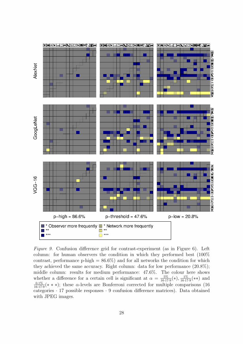
Figure 9. Confusion difference grid for contrast-experiment (as in Figure 6). Leftcolumn: for human observers the condition in which they performed best (100%contrast, performance p-high = 86.6%) and for all networks the condition for whichthey achieved the same accuracy. Right column: data for low performance (20.8%);middle column: results for medium performance: 47.6%. The colour here showswhether a difference for a certain cell is significant at α = 5%

16·17·9(∗), 1%16·17·9(∗∗) and

0.1%16·17·9(∗ ∗ ∗); these α-levels are Bonferroni corrected for multiple comparisons (16categories · 17 possible responses · 9 confusion difference matrices). Data obtainedwith JPEG images.

28

2.0 1.5 1.0 0.5 0.0

0.0

0.2

0.4

0.6

0.8

1.0

Log10 of nominal contrast in percent

Cla

ssifi

catio

n ac

cura

cy

●

●

●

●●

●●●●

AlexNetGoogLeNetVGG−16participants (avg.)

(a) Contrast-experiment accuracy for JPEG im-ages

2.0 1.5 1.0 0.5 0.0

0.0

0.2

0.4

0.6

0.8

1.0

Log10 of contrast in percent

Cla

ssifi

catio

n ac

cura

cy●

●

●

●●

●●●

●

AlexNetGoogLeNetVGG−16participants (avg.)

(b) Contrast-experiment accuracy for PNG im-ages

2.0 1.5 1.0 0.5 0.0

01

23

4

Log10 of nominal contrast in percent

Ent

ropy

of r

espo

nse

dist

ribut

ion

[bits

]

●●●●●●●●

(c) Contrast-experiment entropy for JPEG im-ages

2.0 1.5 1.0 0.5 0.0

01

23

4

Log10 of contrast in percent

Ent

ropy

of r

espo

nse

dist

ribut

ion

[bits

]

●

●●

●●●●●

(d) Contrast-experiment entropy for PNG im-ages

Figure 10. Accuracy and response distribution entropy for contrast-experiment, splitby JPEG and PNG images. (a)(c) Results for JPEG images. N=3, the same threeobservers as for the PNG experiment. (b)(d) Results for PNG images. N=3.

29

0 1 2 3 4 5 6 7

0.0

0.2

0.4

0.6

0.8

1.0

Coherence = 1.0

Log2 of reach

Cla

ssifi

catio

n ac

cura

cy ● ● ●●

●

●

●●

●

AlexNetGoogLeNetVGG−16participants (avg.)

0 1 2 3 4 5 6 7

0.0

0.2

0.4

0.6

0.8

1.0

Coherence = 0.3

Log2 of reach

Cla

ssifi

catio

n ac

cura

cy ● ●●

●

●

● ● ●

0 1 2 3 4 5 6 7

0.0

0.2

0.4

0.6

0.8

1.0

Coherence = 0.0

Log2 of reach

Cla

ssifi

catio

n ac

cura

cy ● ●

●

●

●● ● ●

(a) Classification accuracy

0 1 2 3 4 5 6 7

01

23

4

Coherence = 1.0

Log2 of reach

Ent

ropy

of r

espo

nse

dist

ribut

ion

[bits

]

● ● ● ● ● ● ● ●

0 1 2 3 4 5 6 7

01

23

4

Coherence = 0.3

Log2 of reach

Ent

ropy

of r

espo

nse

dist

ribut

ion

[bits

]● ● ● ●

● ● ● ●

0 1 2 3 4 5 6 7

01

23

4

Coherence = 0.0

Log2 of reach

Ent

ropy

of r

espo

nse

dist

ribut

ion

[bits

]

● ● ● ●● ● ● ●

(b) Response distribution entropy

Figure 11. Complete eidolon-experiment results (n=5). (a) Accuracy including range.This range was obtained as for the other experiments. (b) Response distributionentropy. Note that the data for coherence = 1.0 are already visualized in Figure 3(e) and (f), but are here shown again for better comparison to the results obtainedfor different coherence values.

30

(a) Contrast-experiment, JPEG images (b) Contrast-experiment, PNG images

(c) Eidolon-experiment, coherence = 0.3 (d) Eidolon-experiment, coherence = 0.0

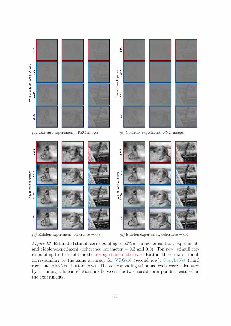
Figure 12. Estimated stimuli corresponding to 50% accuracy for contrast-experimentsand eidolon-experiment (coherence parameter = 0.3 and 0.0). Top row: stimuli cor-responding to threshold for the average human observer. Bottom three rows: stimulicorresponding to the same accuracy for VGG-16 (second row), GoogLeNet (thirdrow) and AlexNet (bottom row). The corresponding stimulus levels were calculatedby assuming a linear relationship between the two closest data points measured inthe experiments.

31