Comparative assessment of energy options and strategies in ... · IAEA-TECDOC-1469 Comparative assessment of energy options and strategies in Mexico until 2025 Final report of a coordinated

IAEA-TECDOC-1469

Comparative assessment ofenergy options and strategies

in Mexico until 2025Final report of a coordinated research project 2000–2004

October 2005

IAEA-TECDOC-1469

Comparative assessment ofenergy options and strategies

in Mexico until 2025Final report of a coordinated research project 2000–2004

October 2005

The originating Section of this publication in the IAEA was:

Planning and Economic Studies Section International Atomic Energy Agency

Wagramer Strasse 5 P.O. Box 100

A-1400 Vienna, Austria

COMPARATIVE ASSESSMENT OF ENERGY OPTIONS AND STRATEGIES IN MEXICO UNTIL 2025

IAEA, VIENNA, 2005 IAEA-TECDOC-1469 ISBN 92–0–111105–3

ISSN 1011–4289 © IAEA, 2005

Printed by the IAEA in Austria October 2005

FOREWORD

Mexico is undergoing significant changes in the energy sector, in particular in the electric power sector, such as the restructuring of power markets; increasing emphasis on socio-economic and environmental impacts of the electric power system; and consideration of an higher role for energy technologies compatible with sustainable development. The Mexican Government has identified the need for ensuring a sustainable pattern of production, distribution and use of energy and electricity. In this context, a comparative assessment analysis is a prerequisite for planning of the future energy and electricity facilities of the country in order to make timely decisions. It requires the identification of the expected levels of energy and electricity demand and the options that are available to meet these demands, taking special note of the national energy resources and potential imported sources. Further analysis would be needed for the optimization of the supply options to meet the demand in the most efficient and economic manner with due consideration of the environmental impacts and resource requirements.

In accordance with its mandate, the IAEA has developed a systematic approach along with a set of computer-based models for elaborating national energy strategies covering the analysis of all of the above aspects. Under its Technical Cooperation Programme, the IAEA provides assistance to its Member States to enhance national capabilities for elaborating sustainable energy development strategies and assessing the role of nuclear power and other energy options, by transferring the analytical tools along with training and providing expertise.

The present report describes the results of the Comparative Assessment of Energy Options and Strategies until 2025 study for Mexico conducted by the Secretaría de Energía, in cooperation with several national institutions, in particular the University of México. The comprehensive national analysis focuses on energy and electricity demand analysis and projections, least-cost electric system expansion analysis, energy resource allocation to power and non-power sectors and environmental analysis.

Because many of the assumptions made for the study are the result of expert consensus but have not been validated or endorsed by the Government, the present study should not be considered as the Energy and Electricity Master Plan for Mexico, but rather as a very real attempt to evaluate the possible evolution of the energy and electricity consumption under certain scenarios of socioeconomic and technical development. Likewise, the expansion plans of the electricity supply system delineated by the study should not be taken as the Government plan in this area. The findings of the study do, however, provide more insight as to the possible strategies for developing the power generating system and the necessary work to be undertaken to supplement the results of the study or to update it, if deviations are experienced in the principal hypothesis made for the study.

It should be noted that the Secretaría de Energía, Mexico, was fully responsible for all phases of the study, including the preparation of the present report. The IAEA’s role was to provide overall coordination and guidance throughout the conduct of the study, and to guarantee that adequate training in the use of IAEA energy planning models was provided to the members of the national team. The IAEA officer responsible for this publication was Kee-Yung Nam of the Department of Nuclear Energy.

EDITORIAL NOTE

The use of particular designations of countries or territories does not imply any judgement by the publisher, the IAEA, as to the legal status of such countries or territories, of their authorities and institutions or of the delimitation of their boundaries.

The mention of names of specific companies or products (whether or not indicated as registered) does not imply any intention to infringe proprietary rights, nor should it be construed as an endorsement or recommendation on the part of the IAEA.

1

CONTENTS

1. SUMMARY...................................................................................................................... 1

1.1. Objectives and scope of the study ...................................................................... 1 1.2. Institutional setup ............................................................................................... 2 1.3. Major assumptions of the study.......................................................................... 3

1.3.1. Demographic assumption ....................................................................... 3 1.3.2. Economic assumption ............................................................................. 3 1.3.3. Energy and environmental policies......................................................... 3

1.4. Energy and electricity demand-supply and emissions results ............................ 4 1.4.1. Reference case scenario results............................................................... 4 1.4.2. Alternative scenario 1 (limited gas supply scenario).............................. 7 1.4.3. Alternative scenario 2 (nuclear scenario) ............................................... 8 1.4.4. Alternative scenario 3 (renewables scenario) ......................................... 9

1.5. Least-cost plan for expansion of the electricity generation system.................... 9 1.6. Others................................................................................................................ 13 1.7. Conclusions ...................................................................................................... 14 1.8. Structure of full report ...................................................................................... 15

2. ECONOMY AND ENERGY ......................................................................................... 17

2.1. Background information................................................................................... 17 2.2. Energy resources............................................................................................... 17

2.2.1. Crude oil reserves ................................................................................. 17 2.2.2. Natural gas reserves .............................................................................. 18 2.2.3. Coal reserves......................................................................................... 20 2.2.4. Uranium reserves .................................................................................. 21 2.2.5. Hydro-electric resources ....................................................................... 21 2.2.6. Geothermal resources ........................................................................... 22 2.2.7. Wind resources ..................................................................................... 25

2.3. Energy supply ................................................................................................... 27 2.3.1. Crude oil production ............................................................................. 30 2.3.2. Natural gas production.......................................................................... 33 2.3.3. Coal production..................................................................................... 35 2.3.4. Uranium production.............................................................................. 36 2.3.5. Hydro-electric capacity and energy production.................................... 36 2.3.6. Geothermal capacity and energy production ........................................ 37 2.3.7. Wind capacity and energy production .................................................. 37

2.4. Energy consumption ......................................................................................... 38 2.4.1. Oil sector (refineries, gas, fractionating plants) energy

consumption.......................................................................................... 39 2.4.2. Power sector capacity, generation and consumption ............................ 40 2.4.3. Power sector capacity ........................................................................... 40 2.4.4. Power sector generation........................................................................ 40 2.4.5. Power sector energy sources consumption ........................................... 41 2.4.6. Power sector transmission lines............................................................ 43 2.4.7. Power sector international commerce................................................... 43 2.4.8. End use sectors energy consumption .................................................... 44 2.4.9. Industrial sector energy consumption ................................................... 46 2.4.10. Residential sector energy consumption ................................................ 47

2

2.4.11. Public and services sector energy consumption ................................... 47 2.4.12. Commercial sector energy consumption............................................... 48 2.4.13. Agricultural sector energy consumption............................................... 49

3. METHODOLOGICAL APPROACH............................................................................. 51

3.1. VALORAGUA Methodology .......................................................................... 51 3.2. WASP Module.................................................................................................. 51 3.3. DECADES methodology.................................................................................. 52 3.4. MODEMA methodology.................................................................................. 53 3.5. BALANCE module of ENPEP......................................................................... 56

4. POWER EXPANSION ALTERNATIVES.................................................................... 61

4.1. Plant-level and system-level analysis ............................................................... 61 4.2. Characterization of existing thermal power plants ........................................... 61

4.2.1. Fuel oil and diesel plants ...................................................................... 61 4.2.2. Coal plants ............................................................................................ 62 4.2.3. Dual plants ............................................................................................ 62 4.2.4. Nuclear power plant.............................................................................. 62 4.2.5. Geothermal plants ................................................................................. 62 4.2.6. Wind plants ........................................................................................... 62

4.3. Engineering data of the power technologies..................................................... 62 4.3.1. Emission factors.................................................................................... 62

4.4. Characterization of existing hydro power plants .............................................. 66 4.5. Characterization of the power plants for the expansion alternatives................ 66 4.6. Projected generation costs of power plants ...................................................... 67

4.6.1. Analysis of power system costs for thermal power plants.................... 67 4.7. Analysis of power system costs for hydro power plants .................................. 68 4.8. Analysis of fuel prices and future escalations .................................................. 70 4.9. Comparison of the expansion alternatives by a screening curves analysis ...... 70 4.10. Projections of electricity demand ..................................................................... 71

4.10.1. Historical evolution of the electricity demand...................................... 71 4.11. Historical system load factors and seasonal variation of peak load ................. 74 4.12. System reserve and reliability........................................................................... 74 4.13. Electricity demand projections used in the study ............................................. 76

4.13.1. Electricity demand projections ............................................................. 76 4.14. Projections of the load curves........................................................................... 78

4.14.1. Assumptions on the system’s reserve and reliability criteria ............... 78 4.15. Input data for the system-level analysis ........................................................... 79

4.15.1. General assumptions ............................................................................. 79 4.15.2. Characterization of existing and firmly committed power plants......... 80 4.15.3. Evolution of the “fixed system” over the study period......................... 83

4.16. Characterization of the power plants for the expansion alternatives................ 83 4.16.1. Parameters for the simulation of the system operation......................... 85 4.16.2. Use of emission abatement technologies .............................................. 87

4.17. System-level analysis of generation system expansion.................................... 87 4.18. Base case analysis............................................................................................. 87

4.18.1. Approach to reach the optimal solution................................................ 87 4.18.2. Analysis of the structure of the power system...................................... 89 4.18.3. Analysis of the power system costs ...................................................... 89 4.18.4. Formulation of the base case findings .................................................. 90

3

4.19. Scenario structure and analysis of expansion alternatives................................ 92 4.19.1. Structure of the scenario alternatives.................................................... 92

4.20. Analysis of the expansion alternatives ............................................................. 94 4.20.1. Impact of lower investment costs for new nuclear power plants.......... 94 4.20.2. Impact of a escalation of natural gas prices .......................................... 97 4.20.3. Impact of a natural gas supply limitation............................................ 102 4.20.4. Impact of a variation of the discount rate ........................................... 106

5. TOTAL ENERGY SYSTEM ANALYSIS................................................................... 109

5.1. Scope of total energy system analysis ............................................................ 109 5.2. Energy network configuration ........................................................................ 111

5.2.1. Conversion, transmission and distribution sectors ............................. 113 5.2.2. Oil refining, gas processing and distribution sectors .......................... 113 5.2.3. Coal and coke production, processing and distribution sectors.......... 118 5.2.4. Nuclear production, processing and distribution sectors .................... 119 5.2.5. Electric power sector .......................................................................... 120

5.3. Demand side sectors ....................................................................................... 125 5.3.1. Industrial demand sector ..................................................................... 127 5.3.2. Residential demand sector .................................................................. 138 5.3.3. Transport demand sector..................................................................... 140 5.3.4. Commercial and public demand sector............................................... 140 5.3.5. Agriculture demand sector.................................................................. 141

6. COMPARATIVE ASSESSMENT ANALYSIS OF ENERGY OPTIONS AND STRATEGIES UP TO 2025 ......................................................................................... 143

6.1. Reference case results..................................................................................... 143 6.1.1. Primary energy supply ........................................................................ 143 6.1.2. Oil and gas sector................................................................................ 143 6.1.3. Electricity supply ................................................................................ 147

6.2. Final energy consumption .............................................................................. 148 6.2.1. Final energy consumption by sector and by fuel ................................ 148 6.2.2. Industrial energy consumption trends................................................. 153 6.2.3. Residential energy consumption trends .............................................. 160 6.2.4. Transportation energy consumption trends......................................... 162 6.2.5. Agriculture energy consumption trends.............................................. 165 6.2.6. Commercial and public energy consumption trends........................... 166

6.3. Net energy exports revenue ............................................................................ 168 6.3.1. Energy imports trends......................................................................... 168 6.3.2. Energy imports trends......................................................................... 169 6.3.3. Environmental results ......................................................................... 170 6.3.4. Emissions of GHG’s ........................................................................... 170 6.3.5. Emissions of CO, SO2, PM and NMVOC .......................................... 176

6.4. Limited gas scenario results ........................................................................... 181 6.4.1. Effects on power sector....................................................................... 181 6.4.2. Effects on supplies .............................................................................. 184 6.4.3. Effects on emissions ........................................................................... 184

6.5. Nuclear scenario results.................................................................................. 188 6.5.1. Effects on power sector....................................................................... 188 6.5.2. Effects on supplies .............................................................................. 188 6.5.3. Effects on emissions ........................................................................... 189

4

6.6. Renewables scenario results ........................................................................... 191 6.6.1. Effects on power sector....................................................................... 191

6.7. Renewables scenario results ........................................................................... 191 6.7.1. Effects on power sector....................................................................... 191 6.7.2. Effects on supplies .............................................................................. 193 6.7.3. Effects on Emissions........................................................................... 193

6.8. Conclusions, recommendations and observations .......................................... 195 6.8.1. Reference case .................................................................................... 196 6.8.2. Energy................................................................................................. 196 6.8.3. Emissions ............................................................................................ 199

6.9. Alternative scenarios ...................................................................................... 200 6.9.1. Limited gas scenario ........................................................................... 200 6.9.2. Energy................................................................................................. 200 6.9.3. Emissions ............................................................................................ 200

6.10. Nuclear Scenario............................................................................................. 201 6.10.1. Energy................................................................................................. 201 6.10.2. Emissions ............................................................................................ 201

6.11. Renewables scenario....................................................................................... 201 6.11.1. Energy................................................................................................. 201 6.11.2. Emissions ............................................................................................ 202

6.12. Additional comments and recommendations ................................................. 202

7. SPECIAL CHAPTER: “COMPARATIVE ASSESSMENT OF ENERGY SOURCES FOR ELECTRICITY SUPPLY UNTIL 2025” ......................................... 205

7.1. Objectives and methodology of the study ...................................................... 205 7.1.1. Overview of the Mexican electric system........................................... 205 7.1.2. Objectives ........................................................................................... 206 7.1.3. Methodology....................................................................................... 207 7.1.4. Modeling approach ............................................................................. 208

7.2. Chain-level analysis........................................................................................ 208 7.2.1. Oil chain.............................................................................................. 210 7.2.2. Crude oil production (Level II)........................................................... 211 7.2.3. Crude oil transportation (Level III) .................................................... 212 7.2.4. Crude oil processing (Level IV) ......................................................... 214 7.2.5. Fuel oil chain (Level IV) .................................................................... 216 7.2.6. Fuel oil transportation (Level V) ........................................................ 217 7.2.7. Fuel oil electricity generation (Level VI) ........................................... 217 7.2.8. Diesel chain (Level IV)....................................................................... 219 7.2.9. Diesel transportation (Level III) ......................................................... 221 7.2.10. Crude oil processing in the diesel chain (Level IV) ........................... 221 7.2.11. Diesel transportation (Level V) .......................................................... 221 7.2.12. Diesel electricity generation (Level VI) ............................................. 222 7.2.13. Natural gas chain ................................................................................ 223 7.2.14. Natural gas production (Level II) ....................................................... 225 7.2.15. Natural gas transportation (Level III) ................................................. 228 7.2.16. Natural gas processing (Level IV) ...................................................... 228 7.2.17. Natural gas transportation (Level V) .................................................. 230 7.2.18. Natural gas electricity generation (Level VI) ..................................... 231 7.2.19. Coal chain ........................................................................................... 231 7.2.20. Coal production (Level II) .................................................................. 232 7.2.21. Coal transportation (Level III) ............................................................ 232

5

7.2.22. Coal preparation (Level IV)................................................................ 232 7.2.23. Coal transportation (Level V) ............................................................. 236 7.2.24. Coal electricity generation (Level VI) ................................................ 238 7.2.25. Nuclear chain ...................................................................................... 238 7.2.26. Nuclear chain emissions ..................................................................... 242 7.2.27. Renewable energy chains.................................................................... 243 7.2.28. Hydroelectric chain............................................................................. 245 7.2.29. Geothermal chain................................................................................ 246 7.2.30. Wind chain.......................................................................................... 251 7.2.31. Elementary comparison of three expansion technologies................... 252

7.3. Decision-making analysis of power system expansion .................................. 254 7.3.1. Applied methodology of decision-making analysis............................ 254 7.3.2. Selection of Alternatives..................................................................... 256 7.3.3. Definition of criteria and criteria weights........................................... 258 7.3.4. Results of the analysis with the DAM Module................................... 263 7.3.5. Pareto analysis .................................................................................... 264 7.3.6. Competition analysis........................................................................... 264 7.3.7. Conclusions of the DAM analysis ...................................................... 266

8. CONCLUSIONS .......................................................................................................... 267

APPENDIX I. ENVIRONMENTAL LEGISLATION AND POLICIES .................. 269

APPENDIX II. ENERGY AND FEEDSTOCK CONSUMPTION............................. 271

APPENDIX III. ENERGY PLANNING AND POLICY IN MEXICO........................ 275

APPENDIX IV. ELECTRICITY PRODUCTION CHAINS FOR OIL AND GAS..... 281

APPENDIX V. MAJOR EMISSIONS......................................................................... 291

APPENDIX VI. NUCLEAR CHAIN COST................................................................. 295

APPENDIX VII. SENSITIVITY ANALYSIS FOR ALTERNATIVE CASES ............ 297

APPENDIX VIII. ENERGY SYSTEM DIVERSITY ..................................................... 299

REFERENCES....................................................................................................................... 301

ACRONYMS AND ABBREVIATIONS .............................................................................. 303

UNITS OF MEASURE.......................................................................................................... 307

CONTRIBUTORS TO DRAFTING AND REVIEW ........................................................... 309

1. SUMMARY

In 1997, the Government of Mexico — the ‘Secretaría de Energía’ (SENER) together with the ‘Comisión Federal de Electricidad’ (CFE) and the ‘Programa Universitario de Energía’ (PUE) of the ‘Universidad Nacional Autónoma de México’ (UNAM) requested to the International Atomic Energy Agency (IAEA) to support in conducting a technical cooperation project to provide SENER, CFE and PUE-UNAM with additional tools for expansion planning of the national electric system, which are necessary for the nation in the evaluation of sustainable growth of the generation capacity in the medium and long term.

In 1998, the IAEA approved the request as a national TC project: MEX/0/012 for the 1999–2000 programme with the title “Comparative Assessment of Energy Sources for Electricity Supply until 2025”. In 2000, the project was extended for 2 years (2001-2002) with a new title “Comparative Assessment of Energy Options and Strategies until 2025” with the objective to broaden the scope and analyze the entire energy system. The first phase of the project was performed using the DECADES software package. The report presents the results of the analysis on the comparative assessment of energy options and strategies until 2025 in entire energy system by using ENPEP (BALANCE) software package while the results of the power system analysis (first phase of the project) was treated as a special chapter of the report.

1.1. Objectives and scope of the study

The general objective of the project is to provide SENER and other Mexican institutions with modern tools that allow in conducting comprehensive comparative assessment of different energy options, supply options as well as total energy system in order to identify sustainable strategies to support the expected growth in energy and electricity demand. This is to be achieved through the acquisition and application of computer-based tools that include environment factors in the assessment of energy systems in addition to traditional economic parameters.

The objectives identified for the study were as follows:

• To project the need for primary energy in Mexico for the period through 2025 that is driven by the expected demand growth for all energy sources;

• To identify domestic supply sufficiency for major energy resources, the long term need for energy imports, and the potential for energy exports;

• To study energy infrastructure development to support the growing energy use in Mexico;

• To analyze, in view of the projected high reliance of the power system and other demand sectors on natural gas, the development of the gas sector in detail in order to identify possible supply constraints, price implications and relevant policy measures:

• To identify the potential role of renewable energy sources in the Mexican energy system;

• To quantify environmental emissions of the whole energy sector associated with the expected growth of energy consumption and possible emission mitigation measures;

1

• To provide, by considering several alternative scenarios, a set of possible scenarios as input to national decision-making in the energy sector.

The scope of the study includes:

• A detailed analysis of overall energy and electricity demand, and its future evolution;

• Assessment of future supply potential of indigenous energy resources - provide, by considering several alternative scenarios, a set of possible scenarios as input to national decision-making in the energy sector;

• Analysis of possibilities of import of various fuels;

• Evolution of future options for electricity generation;

• Formulation of alternative expansion plans for electric sector development; and

• Assessment of environmental impacts of future electricity generation.

1.2. Institutional setup

The study was conceived as a joint effort of Mexico and the IAEA where each part had its own clear and well-established responsibilities:

• Mexican national experts had full responsibility for the conduct of the study, including data collection and preparation, execution of the model runs, interpretation and improvement of results, etc., up to the production of final draft report of the study;

• The IAEA experts provided guidance and cooperation throughout the conduct of the study, on-the-job training of the national team, transfer of know-how and the necessary methodologies and computerized planning tools to Mexico.

The national study team included:

• SENER: Dirección General de Política y Desarrollo de Energéticos

• UNAM: Dirección General de Servicios de Cómputo Académico (both DECADES and ENPEP), Facultad de Ingeniería (both DECADES and ENPEP), and Programa Universitario de Energía (only for DECADES)

• PEMEX: Petróleos Mexicanos

• CFE: Subdirección de Programación

• IIE: Instituto de Investigaciones Eléctricas (only for DECADES)

• INE: Instituto Nacional de Ecología (only for ENPEP)

• IMP: Instituto Mexicano del Petróleo (only for ENPEP)

• CONAE: Comisión Nacional para el Ahorro de Energía (only for ENPEP)

2

SENER defined the objectives to be achieved, invited the relevant institutions to take part, distributed the responsibilities, and coordinated the participation of the teams setup by CFE, UNAM and IIE. SENER, UNAM and IIE collected additional background information needed for the study and the final report. 1.3. Major assumptions of the study

The main assumptions of the study are related with the future evolution of demographic, macroeconomic, social and technological factors, as well as with the national policies on energy and environment. The study period is 1999 to 2025 with 1999 as the base year.

1.3.1. Demographic assumption

The 2000-2025 medium projection population scenario of the National Population Council is used. This population scenario corresponds to annual average growth rates of 1.33% for the period 2000 to 2010, 1.02% for the period 2011 to 2020 and a 0.82% for the last five years of the projection horizon. Under this scenario, Mexico’s population will increase from 98.9 million inhabitants in the year 2000 to 130.2 million inhabitants in the year 2025. Also, under this scenario the participation of the urban population will increase from 75.45% in the year 2000 to 82.3% by 2025 and a reduction of the rural population from 24.55% in the year 2000 to 17.7% by 2025.

1.3.2. Economic assumption

Every year, the Mexican energy sector prepares a set of three economic scenarios with a time span of ten years. Under these economic scenarios, identified as planning scenario, high and moderate the energy sector prepares and publish short and medium term prospective studies for the electricity, natural gas, oil derivatives and liquefied petroleum gas. However, for time spans longer than ten years there is no any official projection for the GDP and the energy demand and supply. Therefore, for the present study, it is assumed an annual GDP average growth rate of 4.5% for the period from 2002 to 2011 and a 3.5% for the period 2012 to 2025. This assumption implies that the portion from 2002 to 2011 corresponds to the planning scenario and for the rest of the time horizon it is assumed that corresponds to the GDP average growth rate of the last 25 years.

1.3.3. Energy and environmental policies

The current energy policy is oriented to provide to the population full access to the energy inputs; to guarantee the supply of energy under competitive conditions of quality and price through world class energy enterprises, public and private, operating within an adequate legal and regulatory framework with high indices of security and respect for the environment; to impulse, strongly, an efficient use of energy as well as to impulse research and development of technology; and a strong promotion and use of renewable energy sources.

Energy and environmental policies are in very close relation and are structured under the principle of sustainable development. The environmental policy, through environmental standards aim to limit the emission of pollutants and induce the intensive use of cleaner fuels, specially in the country areas considered as critical from the environmental point of view.

Energy and environmental policies promote the private inversion on the development of natural gas infrastructure for transport, storage and distribution of this fuel. They reflect the official energy policy, that is, the substitution of fuel oil by natural gas in the power and

3

industrial sectors, the introduction of natural gas in the residential sector and to some extent in the transport sector and the reconfiguration of refineries to produce better gasoline and reduce the production of heavy residuals.

The study covers the areas of crude oil, natural gas, liquefied petroleum gas, oil products, the power sector and the entire Mexican Energy System (domestic production, imports, exports transformation, transportation, distribution and end use). Following the current energy policy and the environmental standards, there is an emphasis on natural gas to replace fuel oil as a result of the current energy policy in the power sector, public and private, to shift power generation from fuel oil to natural gas through the gas-fired combined cycle technology.

To analyze the evolution trends of the energy demand and its supply options the study took the already commented demographic and economic assumptions, the current energy and environmental policies putting emphasis on the fuel substitution and cleaner fuel strategies and develop, for the study, a reference case scenario and three alternative technological scenarios. The set up scenarios are:

• Reference case scenario, corresponding to the assumption of unlimited supply of natural gas, either domestic or imported or both;

• Alternative scenario 1 (limited gas supply scenario), As in the previous scenario all the assumptions are the same as in the reference case scenario, except that assumes a natural gas supply limitation starting 2009, which is equivalent to allow, in the power sector, a maximum of 3 natural gas-fired combined cycle unit per year. For the rest of the sectors and sub-sectors there is no a natural gas supply limitation; and,

• Alternative scenario 2 (nuclear scenario), all the assumptions demographic, economic, energy and environmental policies are identical to the ones established for the reference case scenario, the only difference lies in the power sector through the inclusion of an advance nuclear power plant with a capacity of 1,314 MW;

• Alternative scenario 3 (renewable energy scenario), this scenario focused on the introduction of additional wind and solar PV for power generation. Solar and wind technologies compete with grid electricity on a national level, including the electricity generation isolated system.

1.4. Energy and electricity demand-supply and emissions results

1.4.1. Reference case scenario results

Final energy consumption is projected to grow at an average rate of 3.8% per year, from 4,030 PJ in 1999 to 10,666 PJ by 2025. This growth is strongly fueled by the observed increase in transportation demand, which is projected to grow annually at 4.9% from 1,547 PJ in 1999 to 5,349 PJ in 2025. Transportation accounts for about 57% of the total growth in final consumption (6,636 PJ), making the transport sector the largest consumer by 2025 with over 50% of total final energy consumption (up from 38% in 1999). Industrial demand grows at 3.8% per year, leading to a slight decline in its consumption share from 39% to 37%. By 2025, transport and industry combined account for about 88% of total final energy consumption. Residential energy consumption grows relatively slowly at about 1% annually, leading to a drop in its sectoral share from 17% (1999) to 8% (2025).

4

The model projects refined oil products to continue to play a dominant role in Mexico’s energy future. The share of oil products will remain at approximately 63% throughout the forecast period. Final natural gas consumption grows from 527 PJ to 1,764 PJ (4.8% annually), with the industrial sector accounting for about 90% of the total growth, or 1,114 PJ. The results for the manufacturing sector show energy projections for industrial energy requirements growing from the current 1,561 PJ (1999) to 3,992 PJ (2025). While fuel oil consumption actually declines from 203 PJ in 1999 to 79 PJ in 2025, consumption of other fuels increases, particularly natural gas, which is forecast to continue its penetration of the industrial market. Industrial gas consumption is expected to more than triple from about 500 PJ to 1,615 PJ. Industrial electricity demand is projected to be equally strong, also tripling from 310 PJ to 986 PJ over the forecast period.

Energy projections show a strong growth in transportation energy demand from 1,547 PJ to 5,349 PJ. Motor gasoline and diesel combined will continue to provide 90% of the total transport energy needs, with gasoline accounting for about 63%. Market shares of transportation fuels are forecast to change very little, even that there is a penetration of natural gas and liquefied petroleum gas.

Mexico’s power sector is expected to undergo significant changes over the forecast period. Model results show a dramatically increasing reliance on natural gas for future system expansion. While Mexico’s fuel oil units are either retired or converted to imported coal, natural gas-fired generation increases more than 25 times by 2025. As a result of this development, fuel oil generation decreases from 333 PJ or 92 terawatt-hours (TW·h) in 1999 to 39 PJ (11 TW·h) in 2025, a drop of 88%. Coal generation slightly increases in the early years from 61 PJ (17 TW·h) in 1999 to 106 PJ (29 TW·h) in 2002 and remains at this level throughout the projection period.

Natural gas generation grows at an average rate of 13.2%, from 50 PJ (14 TW·h) in 1999 to 1,265 PJ (351 TW·h) in 2025. By the end of the projection period, gas-fired generation accounts for 79% of total generation (up from 8% in 1999). Hydro and other renewables grow only modestly, leading to a gradual decline in their market share from 22% in 1999 to about 9% in 2025.

Given the strong growth in transport gasoline demand, Mexico’s six refineries are expected to run into their combined capacity limits around 2005. This situation drives up the need for gasoline imports from 196 PJ (1999) to 2,276 PJ (2025), a 12-fold increase equivalent to an annual growth of 9.9%. By 2025, imports supply 66% of Mexico’s gasoline consumption, up from 20% in 1999. If is decided to go through the added value route, then total refining capacity will have to be increased to 1.72 million barrels per day by 2006 up from 1.54 million barrels per day; once the completion of the reconfiguration program of refineries and with a gasoline yielding of 39 percent the total refining capacity will have to reach, in million barrels per day, the following figures: 1.94 in 2008, 2.48 in 2015, 3.16 in 2020 and 4.1 in 2025.

Projected net imports of refined petroleum products also grow. Net imports of refined oil products quickly increase from 215 PJ (1999) to 3,749 PJ (2025). By 2025, net gasoline imports amount to 2,063 PJ, or 55% of total net oil product imports. Net diesel imports are forecast to be 1,098 PJ, or 29% of total net oil product imports. Mexico’s net oil export balance shows the impact of the projected growth in refined product imports. While crude oil exports are expected to continue their growth at an average rate of 0.7% per year from 3,396 PJ in 1999 to 4,520 PJ in 2025, net imports of refined products quickly increase and result in a rapid drop in net oil exports, eventually declining to 771 PJ in 2025, down from a peak of 3,848 PJ in 2005.

5

Total natural gas demand is forecast to grow from 799 PJ (21 billion m3) to 4,678 PJ (127 billion m3) over the projection period. Despite the strong growth in industrial demand (1,114 PJ total growth, or 4.6% per year), the growth in natural gas demand is heavily driven by the power sector dynamics. Natural gas consumption for power generation quickly grows from 273 PJ (7 billion m3) in 1999 to 2,914 PJ (79 billion m3) in 2025, equivalent to a 9.5% annual growth rate and accounting for 68% (2,641 PJ) of the total growth.

Natural gas supply model results shown a rapidly growing demand and is expected to put a strain on the domestic gas supply system. Results indicate the need to develop additional gas fields or rely on increasing gas imports, particularly after 2008 when gas fields currently under development reach their maximum output (domestic non-associated gas). At the same time, associated gas production is projected to slow down as Mexico’s oil refineries reach their combined process capacity, limiting domestic crude oil production (assuming export markets cannot absorb this incremental production). The results are clearly driven by some of the oil and gas sector-specific assumptions, such as (1) total capacity of all gas processing plants remains constant at 5.034 billion ft3 per day, (2) total capacity of all fractionating plants remains constant at 544 million ft3 per day, (3) natural gas exports are marginal and decreasing, and (4) the ratio of crude to associated gas remains constant at the historical level.

It should be noted that according to SENER’s most recent natural gas market analysis (SENER, 2002), PEMEX may substantially increase its natural gas investment program, with the goal of increasing its gas processing capacity, adding new integrated gas processing plants in the Burgos region, expanding its existing fractionating facilities in Coatzacoalcos, and upgrading its pipeline system. Under the accelerated gas development program, domestic natural gas production may increase substantially to almost 9.0 billion ft3 per day by 2010 and thereby significantly alter the results above. This issue may be analyzed in more detail in subsequent model runs.

In addition, the study reported here did not attempt to investigate different sources of imported gas or whether it will be in the form of liquefied natural gas (LNG) and where these LNG terminals will likely be located. Undoubtedly though, if Mexico will not be able to close the projected gap between supply and demand either from additional domestic supplies or new imports, it might be exposed to price volatility similar to what has been observed in the United States recently (Greenspan, 2003) or risk disruptions in its gas markets. For a more detailed discussion and additional analysis we refer to the reader to Chapter 5 of this report.

Carbon dioxide (CO2) emissions are forecast to grow at an average annual rate of 3.4% from 346 million metric tons (Mt) in 1999 to 828 Mt in 2025. Transportation-related emissions grow the fastest at 4.9% per year from 108 Mt to 371 Mt over the forecast period, accounting for 55% of the total growth in CO2 emissions. By 2025, the transport sector is responsible for 45% of Mexico’s CO2 emissions (up from 31% in 1999), followed by the power sector with 193 Mt and 23% (up from 98 Mt and 28%) and industry with 147 Mt and 18% (up from 58 Mt and 17%). The 5% drop in the power sector share is related to the rapidly growing penetration of natural gas as an energy source in that sector.

National emissions of nitrogen oxides (NOX) are projected to increase from 1.52 Mt (1999) to 4.61 Mt (2025), equivalent to a 4.4% growth rate. This development is closely linked to transport sector dynamics, as the sector contributes about 77%, or 2.38 Mt, to the overall growth in NOX emissions. The transport share remains very high and gradually increases from 67% to 74% through the forecast period. The power sector, the second largest source, contributes 282 kilotons (kt) or about 19% in 1999 and 837 kt or about 18% in 2025.

6

The projected sulfur dioxide (SO2) emissions exhibit a marked reduction of about 24% from 1999 to 2025. Emissions are forecast to initially decline from 2.35 Mt (1999) to a low of 1.21 Mt (2008) and then gradually increase again to 1.78 Mt (2025). The most notable change is the substantial drop in power sector emissions from 1.71 Mt (73% of the total) in 1999 to 0.38 Mt (22% of the total) in 2025. This drop is linked to the retirement of several of Mexico’s fuel oil units burning high-sulfur fuel oil, the conversion of some of the fuel oil units to low-sulfur imported coal plants, and the projected dramatic switch to natural gas for power generation with essentially zero SO2 emissions. The gradual increase in national SO2 emissions after 2008 is related to the rise in industrial SO2 emissions, which grow on average at about 3.4% from 0.44 Mt in 1999 to 1.07 Mt in 2025 as the sector continues to burn high-sulfur fuel oil. This situation causes the manufacturing sector to become the largest source of SO2 by the end of the analysis period, contributing 60% of SO2 emissions as compared to 19% in 1999.

The behavior of projected emissions of particulate matter (PM) is somewhat comparable with the previous discussion for SO2 in that emissions initially decline from 323 kt (1999) to 280 kt (2003) and then increase to 484 kt (2025). However, the drop in power-sector PM emissions is not nearly enough to offset the continued emissions growth in the other sectors, therefore leading to an overall increase in PM emissions. While power sector PM emissions decline from 92 kt (29% of total, largest PM source) in 1999 to 19 kt (4% of total) in 2025, emissions in other sectors, particularly the transport and industrial sectors, continue to grow. By 2025, transportation is the largest PM source, with 208 kt or 43% of the total (up from 60 kt or 18% of the total in 1999).

1.4.2. Alternative scenario 1 (limited gas supply scenario)

The limitation of the gas supply for power generation changes the expected expansion of the power sector substantially. Starting in 2009, the expansion model selects the maximum of three combined cycle units each year instead of three to seven units per year under the Reference Case. The cumulative number of combined cycle units under the Limited Gas Scenario is 85 or 44.8 gigawatts (GW) as compared to 118 units (62.2 GW) under the Reference Case.

Respect to the effect on generation by fuel type it is noteworthy that while the gas limitation becomes effective in 2009, the generation results do not show a significant difference until 2014, the year when WASP/DECADES projects the first coal-fired units to come on-line. During 2009 to 2013, even though there are four combined cycle units less than in the Reference Case, new coal units are not needed until 2014. Starting in 2014, the model projects between four and six coal-fired units to come on-line each year, with a total of 57 coal units or 17.7 GW. Correspondingly, coal generation starts to increase quickly from 106 PJ (29 TW·h) in 2013 to 572 PJ (159 TW·h) by 2025, accounting for 36% of total power generation. The increased coal generation essentially replaces up to 470 PJ of gas-fired generation by 2025. The share of natural gas generation, therefore, reaches only about 50%, compared to 79% under the Reference Case.

The lower gas generation noticeably slows the growth in total natural gas consumption. Gas consumption is expected to grow to 3,710 PJ, down from 4,678 PJ in the Reference Case. This reduction of 968 PJ or 21% is essentially because of reduced power sector gas demand. Under the Reference Case, the power sector accounts for about 68% of total natural gas demand, but under the Limited Gas Scenario, this share is down to 53%.

7

In response to the reduction in gas demand for power generation, the need for new natural gas sources/imports declines. While approximately 2,690 PJ of gas has to be added/imported in the Reference Case by 2025, imports are down to 1,781 PJ under this scenario. The additional coal-fired generation cannot address the near- to intermediate-term natural gas needs. Additions/imports are substantially reduced only starting in 2014. The decrease of 909 PJ by 2025 is equivalent to a 34% reduction of natural gas imports.

At US$709.58 billion in net present value, the total economic system cost is higher than under the Reference Scenario; that is, a limitation on natural gas supply comes at an economic cost, in this case estimated to be an incremental cost of US$2.17 billion.

Not surprisingly, the shift from gas to coal comes at an environmental cost as well. Atmospheric emissions are projected to increase under the Limited Gas Scenario. For example, the changes in CO2 and NOX emissions compared to the Reference Case. Under the Limited Gas Scenario, power sector CO2 emissions grow to 239 Mt, while total national emissions reach 874 Mt. This increase is about 46 million tons more than the Reference Case, equivalent to a 24% increase in power sector emissions, or 5.5% of national CO2 emissions. Emissions of NOX exhibit a similar behavior in that power sector emissions are forecast to reach about 990 kt by 2025, which is about 152 kt, or 18%, higher than under the Reference Case.

1.4.3. Alternative scenario 2 (nuclear scenario)

On the basis of a capital cost of US$ 2,485.4 for the nuclear candidate the expansion of the power sector does not include, in any case, this technology. Capital cost for this technology to enter into the expansion has to be lowered, for about a 48%. Under this capital cost reduction five new nuclear power plants appear in the optimal solution for the expansion of capacity. Nevertheless, in order to see the non-economic advantages of this technology, a scenario of a forced nuclear introduction was considered. This scenario includes a forced nuclear power plant of 1,356 MW and its objective was to see the non-economic advantages of this technology, such as, lower emissions or a more diversified power system, and its impact on the system cost.

Because of the large capacity of the nuclear unit, the expansion schedule is slightly affected starting in 2001 even though the unit is not coming on-line until 2012. This leads to some minor changes in generation and fuel consumption in the power sector between 2001 and 2011 in comparison with the Reference case scenario. Specifically, from 2001 up to 2011 there is an additional participation of fuel oil generation, which decreases along the years and ends by 2011; hydro also participates with an additional generation, but its participation is just during the year 2001; also there is a declining reduction in the participation of natural gas in the generation along those years. During the years 2009 to 2011 the fuel type mix in the power generation keeps the reference case structure. When the nuclear unit does come on-line, it is base-loaded into the system and generates a constant level of 34 PJ of electricity per year equivalent to 1.5 percent of total generation in 2025 as compared to 1.1 percent under the reference case scenario. The system-level analysis shows that nuclear replaces effectively base-loaded gas combined-cycle capacity and between 33-37 PJ of gas-fired generation.

As with the previous scenarios, the shift away from gas-fired generation leads directly to a reduction in natural gas imports. In this case, gas imports are cut by 63-71 PJ or 2.3 percent by 2025. At US$707.69 billion in net present value, total economic system cost is higher than under the reference scenario, that is, an incremental cost of US$273.4 million.

8

The minor changes in dispatch in the early years lead to small emissions increases of up to 1.2 million tons per year in 2003. But emissions are noticeable reduced starting in 2012 when the nuclear unit eventually comes on-line. For example, CO2 emissions reductions vary between 3.6 and 4.0 million ton per year, equivalent to a 1.9 percent reduction in power sector emissions and a 0.4 percent reduction in national emissions. Total cumulative emissions reductions are 47.5 million ton of CO2. The cost-effectiveness of nuclear technology as a GHG mitigation technology is therefore US$5.8/ton CO2. A similar behavior is exhibited by NOX, N2O, SO2 and PM emissions with a cumulative effect of 228,000 ton for NOX emissions, 60.3 ton for N2O, 242,790 ton for SO2 and 14,320 ton for PM emissions along the entire period. The environmental effects and the cost reductions of this technology should be an area of future investigations.

1.4.4. Alternative scenario 3 (renewables scenario)

Because of the relative costs of wind and solar, the role of solar PV will be very limited. By 2025, solar will generate only about 1.2 PJ of electricity or 0.1 percent of total generation. This is equivalent to 195 MW of installed PV capacity. Wind, on the other side, is forecast to penetrate the market relatively rapidly. This energy source is forecasted that will account for approximately 4.9 percent of total generation, that is, 78.3 PJ by 2025. At the assumed average capacity factor of 26.2 percent, about 9,500 MW of wind capacity will be needed to generate this power. Wind will essentially replace marginal gas-fired generation by up to 93.3 PJ (2025), that is, about 19 percent more than wind electricity. The main reason for this difference is the underlying model implementation which assumes that wind generation will be more dispersed, closer to actual loads, and therefore not subject to the transmission and distribution losses in the electric grid.

Because of the change in generation mix originated by the incorporation of wind energy, the power sector will require less natural gas. This translates directly into less natural gas imports. The reduction in gas imports grows as wind generation increases and reaches approximately 180 PJ by 2025. At US$707.87 billion in net present value, total economic system cost is higher than under the reference scenario, that is, an incremental cost of US$455.64 million.

Since solar and wind replace electricity that is generated mostly by gas-fired combined cycle units limits the emission reduction potential of renewable technologies. NOX emissions, for example, are 44,000 ton per year (2025) below projected reference case scenario levels. This is equivalent to a 5.5 percent drop in power sector emissions and a 1.0 percent decrease of total national NOX emissions. Cumulative NOX reductions over 2005-2025 total about 351,000 ton. The combined effect of technologies, solar PV and wind, through an accelerated penetration of renewable power generation results in CO2 emissions that are up 10 million ton per year (2025) below the reference case scenario levels. This represents a 5.4 percent decrease in power sector CO2 emissions and a 1.2 percent decrease of total national CO2 emissions. The total cumulative emissions reductions in the period from 2005 to 2025 are equal 81.96 million ton. The cost-effectiveness of solar and wind as a GHG mitigation technology is therefore US$5.6/ton CO2. This value is likely to be lower if we ignore the more expensive solar technologies and include only wind in the model. This should be an area of future investigations.

1.5. Least-cost plan for expansion of the electricity generation system

For the expansion of the power system in the near future is expected an increase in the use of oil products, mainly natural gas, because of the low investment costs of the combined cycle

9

plants and their conversion efficiency, as well as for environmental aspects. This expansion policy aims to minimize the dependency of imported sources of energy, for example, coal, if dual plants were installed. Also, in the middle term, some hydro projects are considered as expansion candidates, despite of their high investment costs, but with the purpose of an increasing level in the use of the hydro resources, to diversify the system generation expansion and to take into account environmental aspects. The expansion of the electric system was carried out taking into account these considerations and the technical and economic parameters explained in Chapter 2.

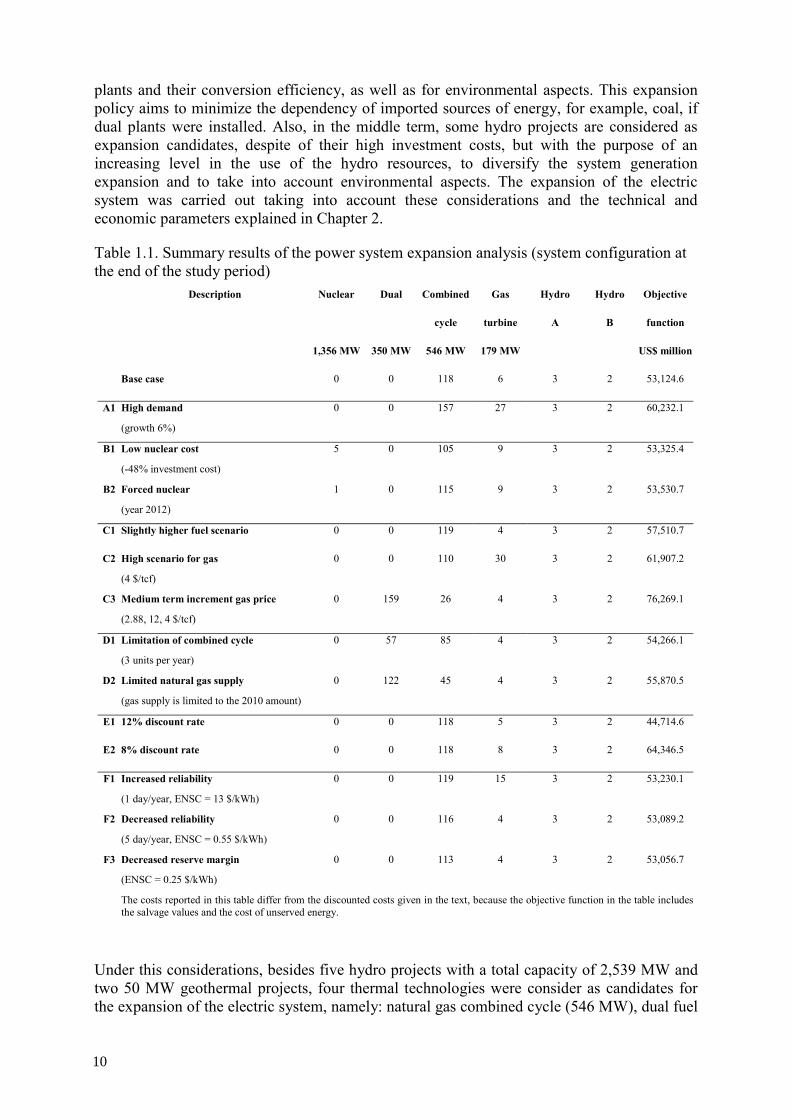
Table 1.1. Summary results of the power system expansion analysis (system configuration at the end of the study period)

Description Nuclear Dual Combined Gas Hydro Hydro Objective

cycle turbine A B function

1,356 MW 350 MW 546 MW 179 MW US$ million

Base case 0 0 118 6 3 2 53,124.6

A1 High demand

(growth 6%)

0 0 157 27 3 2 60,232.1

B1 Low nuclear cost

(-48% investment cost)

5 0 105 9 3 2 53,325.4

B2 Forced nuclear

(year 2012)

1 0 115 9 3 2 53,530.7

C1 Slightly higher fuel scenario 0 0 119 4 3 2 57,510.7

C2 High scenario for gas

(4 $/tcf)

0 0 110 30 3 2 61,907.2

C3 Medium term increment gas price

(2.88, 12, 4 $/tcf)

0 159 26 4 3 2 76,269.1

D1 Limitation of combined cycle

(3 units per year)

0 57 85 4 3 2 54,266.1

D2 Limited natural gas supply

(gas supply is limited to the 2010 amount)

0 122 45 4 3 2 55,870.5

E1 12% discount rate 0 0 118 5 3 2 44,714.6

E2 8% discount rate 0 0 118 8 3 2 64,346.5

F1 Increased reliability

(1 day/year, ENSC = 13 $/kWh)

0 0 119 15 3 2 53,230.1

F2 Decreased reliability

(5 day/year, ENSC = 0.55 $/kWh)

0 0 116 4 3 2 53,089.2

F3 Decreased reserve margin

(ENSC = 0.25 $/kWh)

0 0 113 4 3 2 53,056.7

The costs reported in this table differ from the discounted costs given in the text, because the objective function in the table includesthe salvage values and the cost of unserved energy.

Under this considerations, besides five hydro projects with a total capacity of 2,539 MW and two 50 MW geothermal projects, four thermal technologies were consider as candidates for the expansion of the electric system, namely: natural gas combined cycle (546 MW), dual fuel

10

with desulphurization (350 MW), natural gas simple cycle (179 MW) and advanced nuclear water reactors (1,356 MW).

The main reason for the choosing of these alternatives for the expansion of the Mexican Electric System is the economic factor. However, other aspects become also important for the development of the power plant expansion of the electric system. Aspects, such as environmental impacts (e.g. lower CO2 emissions with nuclear plants), oil derivatives and natural gas prices and energy supply diversification have an effect on the economic factor and were considered in the analysis.

DECPAC module (WASP-III Plus version) of DECADES has been used to carry out the analysis of the base case and several different alternative plans for the future expansion of the power system over 27 years; the planning period is from 1999 to 2025.

Table 6.2 shows the results for the reference case and 13 alternatives evaluated in the system level analysis. The reference case optimal solution until 2025 for the expansion of the electric system requires the installation of 118 natural gas -fired combined cycle units (64,428 MW), 6 gas-fired turbines (1,074 MW), as well as 2,539 MW of hydro projects, with a total discounted cost of US$54.4 billion, US$9.5 billion for capacity additions and US$44.9 billion for operation and maintenance.

The cases that have the higher impact with respect to the reference case are those of higher escalation of natural gas prices. In alternative C1 (slightly higher fuel prices), the number and type of units to be installed are essentially the same as in the base case, because it requires 119 gas-fired combined cycle units (64,974 MW) and 4 gas-fired turbine units (716 MW). The total discounted cost increases to US$58.8 billion, US$ 9.7 billion for investment in capacity additions and US$49.1 billion for operation and maintenance.

In alternative C2 (high natural gas price), 110 gas-fired combined cycle units (60,060 MW) and 30 gas-fired turbine units (5,370 MW) are required, but the total discounted cost increases significantly to US$63.2 billion, US$8.9 billion for investment in capacity additions and US$54.3 billion for operation and maintenance.

For alternative C3 (medium term increase in the gas price) the mix of new units changes considerably compared to the reference case. Only 26 gas-fired combined cycle units (14,196 MW) and 4 gas-fired turbine units (716 MW) are required, but they must be complemented by 159 coal-fired dual units (55,650 MW) with a very substantial increase in the total discounted cost, US$79.6 billion of which US$27.7 billion are for capacity additions and US$52.0 for operation and maintenance.

With regard to the impact of the natural gas supply limitation scenario, alternative D1 (limitation on number per year of new gas-fired combined cycle) the number of gas-fired combined cycle units required is limited to 85 (46,410 MW), the number of gas-fired turbine units is reduced to 4 (716 MW), but the system expansion requires the construction of 57 coal-fired dual units (19,950 MW). The total discounted cost increases to US$56.5 billion, US$12.0 billion for investment in capacity additions and US$44.5 billion for operation and maintenance.

On the other hand, under the natural gas supply limitation scenario, alternative D2 (limited gas supply starting 2010), the number of gas-fired combined cycle and gas-fired turbine units are restricted to 45 (24,570 MW) and 4 (716 MW) units, respectively, but the number of coal-fired dual units is increased to 122 (42,700 MW). The total discounted cost increases to

11

US$59.2 billion; the investment cost increases to US$15.5 and the operation and maintenance cost is reduces to US$43.8 billion.

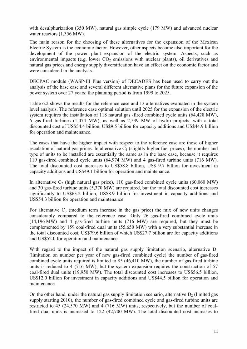
Table 1.2. Emissions from the alternatives of the power system expansion at the last year of the study period.

Description CO2 SOX NOX PM

million ton thousand ton thousand ton thousand ton

Base case 196 344 338 16.3

A1 High demand

(growth 6%)

251 378 409 18.3

B1 Low nuclear cost

(-48% investment cost)

177 357 315 17.0

B2 Forced nuclear

(year 2012)

192 353 334 16.8

C1 Slightly higher fuel scenario 195 326 336 15.2

C2 High scenario for gas

(4 $/tcf)

205 845 361 46.4

C3 Medium term increment gas price

(2.88, 12, 4 $/tcf)

323 630 1,192 58.3

D1 Limitation of combined cycle

(3 units per year)

241 444 646 31.2

D2 Limited natural gas supply

(gas supply is limited to the 2010 amount)

293 590 999 50.2

E1 12% discount rate 196 344 338 16.3

E2 8% discount rate 196 344 338 16.2


(1 day/year, ENSC = 13 $/kWh)

195 327 336 15.2


(5 day/year, ENSC = 0.55 $/kWh)

197 395 341 19.3


(ENSC = 0.25 $/kWh)

198 477 346 24.3

ENSC = cost of unserved energy

The impact of lower investment cost for nuclear units, alternative B1, introduces 5 new nuclear units (6,780 MW) in the expansion of the electric system, 105 gas-fired combined

12

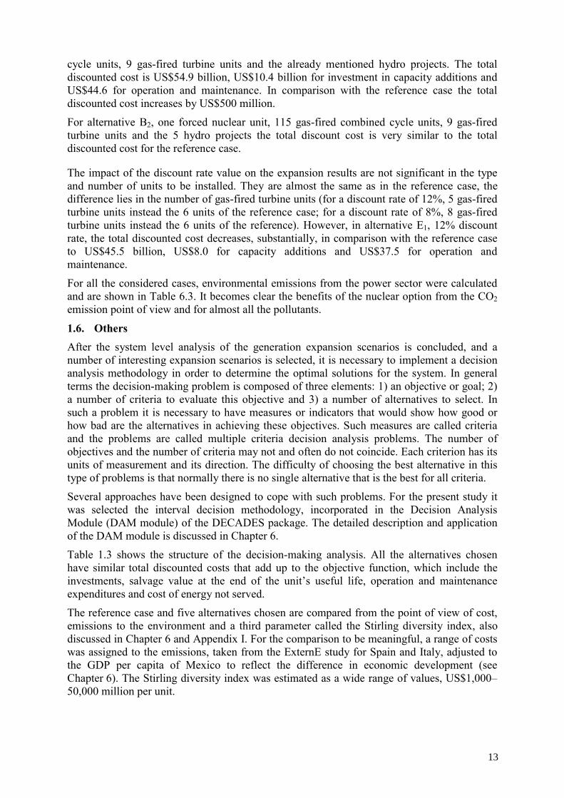
cycle units, 9 gas-fired turbine units and the already mentioned hydro projects. The total discounted cost is US$54.9 billion, US$10.4 billion for investment in capacity additions and US$44.6 for operation and maintenance. In comparison with the reference case the total discounted cost increases by US$500 million.

For alternative B2, one forced nuclear unit, 115 gas-fired combined cycle units, 9 gas-fired turbine units and the 5 hydro projects the total discount cost is very similar to the total discounted cost for the reference case.

The impact of the discount rate value on the expansion results are not significant in the type and number of units to be installed. They are almost the same as in the reference case, the difference lies in the number of gas-fired turbine units (for a discount rate of 12%, 5 gas-fired turbine units instead the 6 units of the reference case; for a discount rate of 8%, 8 gas-fired turbine units instead the 6 units of the reference). However, in alternative E1, 12% discount rate, the total discounted cost decreases, substantially, in comparison with the reference case to US$45.5 billion, US$8.0 for capacity additions and US$37.5 for operation and maintenance.

For all the considered cases, environmental emissions from the power sector were calculated and are shown in Table 6.3. It becomes clear the benefits of the nuclear option from the CO2 emission point of view and for almost all the pollutants.

1.6. Others After the system level analysis of the generation expansion scenarios is concluded, and a number of interesting expansion scenarios is selected, it is necessary to implement a decision analysis methodology in order to determine the optimal solutions for the system. In general terms the decision-making problem is composed of three elements: 1) an objective or goal; 2) a number of criteria to evaluate this objective and 3) a number of alternatives to select. In such a problem it is necessary to have measures or indicators that would show how good or how bad are the alternatives in achieving these objectives. Such measures are called criteria and the problems are called multiple criteria decision analysis problems. The number of objectives and the number of criteria may not and often do not coincide. Each criterion has its units of measurement and its direction. The difficulty of choosing the best alternative in this type of problems is that normally there is no single alternative that is the best for all criteria.

Several approaches have been designed to cope with such problems. For the present study it was selected the interval decision methodology, incorporated in the Decision Analysis Module (DAM module) of the DECADES package. The detailed description and application of the DAM module is discussed in Chapter 6.

Table 1.3 shows the structure of the decision-making analysis. All the alternatives chosen have similar total discounted costs that add up to the objective function, which include the investments, salvage value at the end of the unit’s useful life, operation and maintenance expenditures and cost of energy not served.

The reference case and five alternatives chosen are compared from the point of view of cost, emissions to the environment and a third parameter called the Stirling diversity index, also discussed in Chapter 6 and Appendix I. For the comparison to be meaningful, a range of costs was assigned to the emissions, taken from the ExternE study for Spain and Italy, adjusted to the GDP per capita of Mexico to reflect the difference in economic development (see Chapter 6). The Stirling diversity index was estimated as a wide range of values, US$1,000–50,000 million per unit.

13

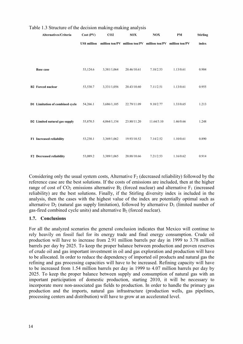
Table 1.3 Structure of the decision making-making analysis Alternatives/Criteria Cost (PV) CO2 SOX NOX PM Stirling

US$ million million ton/PV million ton/PV million ton/PV million ton/PV index

Base case 53,124.6 3,381/1,064 20.46/10.61 7.18/2.53 1.13/0.61 0.904

B2 Forced nuclear 53,530.7 3,331/1,056 20.43/10.60 7.11/2.51 1.13/0.61 0.955

D1 Limitation of combined cycle 54,266.1 3,686/1,105 22.79/11.09 9.10/2.77 1.33/0.65 1.213

D2 Limited natural gas supply 55,870.5 4,064/1,154 23.80/11.20 11.64/3.10 1.46/0.66 1.248

F1 Increased reliability 53,230.1 3,369/1,062 19.93/10.52 7.14/2.52 1.10/0.61 0.890

F2 Decreased reliability 53,089.2 3,389/1,065 20.88/10.66 7.21/2.53 1.16/0.62 0.914

Considering only the usual system costs, Alternative F2 (decreased reliability) followed by the reference case are the best solutions. If the costs of emissions are included, then at the higher range of cost of CO2 emissions alternative B2 (forced nuclear) and alternative F1 (increased reliability) are the best solutions. Finally, if the Stirling diversity index is included in the analysis, then the cases with the highest value of the index are potentially optimal such as alternative D2 (natural gas supply limitation), followed by alternative D1 (limited number of gas-fired combined cycle units) and alternative B2 (forced nuclear).

1.7. Conclusions

For all the analyzed scenarios the general conclusion indicates that Mexico will continue to rely heavily on fossil fuel for its energy trade and final energy consumption. Crude oil production will have to increase from 2.91 million barrels per day in 1999 to 3.78 million barrels per day by 2025. To keep the proper balance between production and proven reserves of crude oil and gas important investment in oil and gas exploration and production will have to be allocated. In order to reduce the dependency of imported oil products and natural gas the refining and gas processing capacities will have to be increased. Refining capacity will have to be increased from 1.54 million barrels per day in 1999 to 4.07 million barrels per day by 2025. To keep the proper balance between supply and consumption of natural gas with an important participation of domestic production, starting 2010, it will be necessary to incorporate more non-associated gas fields to production. In order to handle the primary gas production and the imports, natural gas infrastructure (production wells, gas pipelines, processing centers and distribution) will have to grow at an accelerated level.

14

Natural gas will be the primary choice for power system expansion and generation leading to a near term and long term need for additional gas imports (or accelerated expansion of natural gas domestic production). Under restricted conditions of financial sources natural gas and environmental policies should be review and fuel oil generation incorporated and analyzed their benefits in the short and medium term.

In the case of the nuclear option specific studies will have to carry out. Special attention has to be paid to the total cost of the expansion scenarios including the internalization of the environmental externalities of the whole energy chain and looking for the total cost at which the nuclear option becomes competitive.

An additional conclusion derived from the study is the need for SENER, CFE and UNAM to analyze with much more detail the issue of economic, environmental, social and political impact of the diversification of the mix of technologies for the long term expansion of the electric system in Mexico as well as for the entire Mexican energy system. This conclusion arises from the vulnerability that exists in case of limitations in the supply of natural gas or in the increase of their prices.

In the context of diversification it can be recommended that SENER, CFE and UNAM study the possible economic and environmental benefits of incorporating more wind, solar and geothermal units as candidate technologies for the expansion of the electric system and alternative technologies in the other sectors of the Mexican energy system. The results of these studies could indicate the need to incorporate wind and solar technologies in the COPAR document of CFE as well as in the outlook of the electric sector published by SENER ([5] del Sector Eléctrico). On the other hand, at the level of the integrated Mexican energy system the need for the study of the possible economic and environmental costs and benefits of incorporating new technologies for transportation, industrial process and final end uses in the different sector of the energy system.

From the point of view of the model’s structure and it use, there is also a need to increase energy data availability and quality in the all the sectors. This is strictly necessary in order to improve the results of the model and the benefits of its use. Significant efforts are to be done in the characterization of the different conversion processes used in the industrial and other sectors. It is urgent to improve availability and reliability of the information related to energy efficiency, costs, final end uses, input/output ratios for different processes and final end uses, etc. This could be achieved by providing information, sources of information, accessibility to the information and a compromise of confidential and correct use of the provided information.

1.8. Structure of full report

The full report of project MEX/0/012 consists of this summary, five chapters and several Appendixes. They were written by different participants in the project and were compiled under the direction and supervision of SENER, UNAM and IAEA.

The first chapter summarizes the objectives and scope of the study, assumptions for the analysis as well as the results of the study. Chapter two incorporates reference information useful to readers of the report not familiar with Mexico and its energy sector. Chapter three describes the methodologies, which were used in the study. Chapter four summarizes the result of the WASP (/DECADES) study on power system alternatives of expansion with consideration of the environmental impacts related to different energy technologies. Chapters five and six refer to the conducted study on comparative assessment of energy options and

15

strategies for the total energy system in Mexico by using ENPEP software package and MODEMA. Chapter five explains the scope of the study and the configuration of the entire energy network while Chapter six deals with its main results. Chapter seven, as a special chapter, refers to the results of the DECADES study, namely system level analysis and decision-making analysis. The last chapter contains conclusion and recommendations. The Appendixes contain additional information related to the tasks of the project.

16

2. ECONOMY AND ENERGY

2.1. Background information

Mexico is located in the northern part of the American Continent, together with Canada and United States; but often grouped into the Latin America region. Mexico is adjacent in its northern part with the United States and southeastern part with Guatemala and Belize. The total area accounts 1,964,375 km² - 1,959,248 km² of continental surface and 5,127 km² of the insular surface.

Mexico’s total population in 2000 was 98.9 million, ranked the eleventh position in the world with the annual average growth rate of 1.7% between 1990 and 2000.

Over the past few years, Mexico’s economy showed slow growth and in 1999, Gross Domestic Product (GDP) accounted to 483.7 billion US$, where the agricultural sector represented 5.0% of the percentage share, while industry and service sector represented 28.2% and 66.8%, respectively. Within the industry sector, manufacturing accounted 74.7%. The energy sector has played a key role in Mexican economic development by providing sufficient, reliable and low cost industrial inputs, as well as goods and services for consumers. Throughout the years the energy sector has also consolidated itself as a very important foreign currency generator.

2.2. Energy resources

Mexico is rich in natural energy resources with crude oil, natural gas, coal, uranium and renewable energy sources such as hydro, geothermal, wind and others. Of these, crude oil and gas are, by all means, the most important in energy sources where Mexico ranks the seventh and twenty-first position in the world for proven crude oil and natural gas reserves, respectively.

2.2.1. Crude oil reserves

Mexico’s total oil reserves (proved, probable and possible), in terms of crude oil, gas liquids and expressed in barrels of oil equivalent, are shown in Table 2.1.

Total oil reserves are located in four regions, two marine regions and two onshore regions. Marine regions are located in the Gulf of Mexico and the onshore regions are located in the south and north parts of the continental land.

In the beginning of year 2002, marine regions (Northeastern and Southwestern) represent 52.2% of the total crude oil reserves, while onshore regions (Southern and Northern regions) the remaining 47.8%. In terms of total gas liquids reserves the splitting between these regions are 39.25 and 60.75%, respectively.

Crude oil reserves of the Northeastern Marine and North Regions consist of heavy1 and light2 oil. Oil from the Southwestern Marine Region consists of light oil and from the South Region are heavy, light and lighter3 oil.

1 Crude oil with American Petroleum Institute Classification (API) density less or equal than 27° - mainly produced in the

Campeche Sound. 2 Crude oil with API density between 27° and 38° - produced in the Campeche Sound and other areas. 3 Crude oil with API density higher than 38° - produced in the Mesozoic areas of the Southern Region.

17

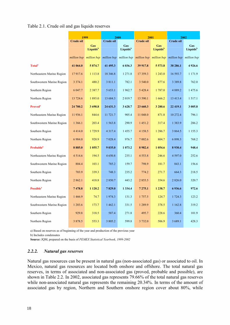
Table 2.1. Crude oil and gas liquids reserves

1999 2000 2001 2002 Crude oil

Gas Crude oil

Gas Crude oil

Gas Crude oil

Gas Liquidsb Liquidsb Liquidsb Liquidsb

million bep million bep million bep million bep million bep million bep million bep million bep

Totala 41 064.0 5 874.7 41 495.3 6 036.3 39 917.8 5 573.8 38 286.1 4 926.6

Northeastern Marine Region 17 917.6 1 113.8 18 346.8 1 271.8 17 359.3 1 243.0 16 593.7 1 171.9

Southwestern Marine Region 3 374.1 480.2 3 811.1 782.1 3 540.0 877.6 3 389.8 762.0

Southern Region 6 047.7 2 387.7 5 653.1 1 962.7 5 428.4 1 787.0 4 889.2 1 475.6

Northern Region 13 724.6 1 893.0 13 684.3 2 019.7 13 590.1 1 666.2 13 413.4 1 517.1

Proveda 24 700.2 3 698.8 24 631.3 3 628.7 23 660.3 3 280.6 22 419.1 3 005.8

Northeastern Marine Region 11 936.1 844.6 11 721.7 905.4 11 048.0 871.8 10 272.4 796.1


Southern Region 4 414.0 1 729.9 4 317.4 1 455.7 4 158.5 1 286.7 3 864.5 1 155.3

Northern Region 6 984.0 920.9 7 028.4 976.7 7 002.6 804.7 6 898.3 768.2

Probablea 8 885.0 1 055.7 9 035.0 1 073.2 8 982.4 1 054.6 8 930.4 948.4


Southwestern Marine Region 804.4 103.1 785.2 159.7 798.9 181.7 843.1 156.6

Southern Region 703.9 339.3 748.3 235.2 774.2 271.7 664.3 218.5

Northern Region 2 862.1 418.8 2 850.7 443.2 2 855.5 354.6 2 826.0 320.7

Possiblea 7 478.8 1 120.2 7 829.0 1 334.4 7 275.1 1 238.7 6 936.6 972.6



Southern Region 929.8 318.5 587.4 271.8 495.7 228.6 360.4 101.9

Northern Region 3 878.5 553.3 3 805.2 599.8 3 732.0 506.9 3 689.1 428.3

a) Based on reserves as of beginning of the year and production of the previous year b) Includes condensates Source: JQM, prepared on the basis of PEMEX Statistical Yearbook, 1999-2002

2.2.2. Natural gas reserves

Natural gas resources can be present in natural gas (non-associated gas) or associated to oil. In Mexico, natural gas resources are located both onshore and offshore. The total natural gas reserves, in terms of associated and non-associated gas (proved, probable and possible), are shown in Table 2.2. In 2002, associated gas represents 79.66% of the total natural gas reserves while non-associated natural gas represents the remaining 20.34%. In terms of the amount of associated gas by region, Northern and Southern onshore region cover about 80%, while

18

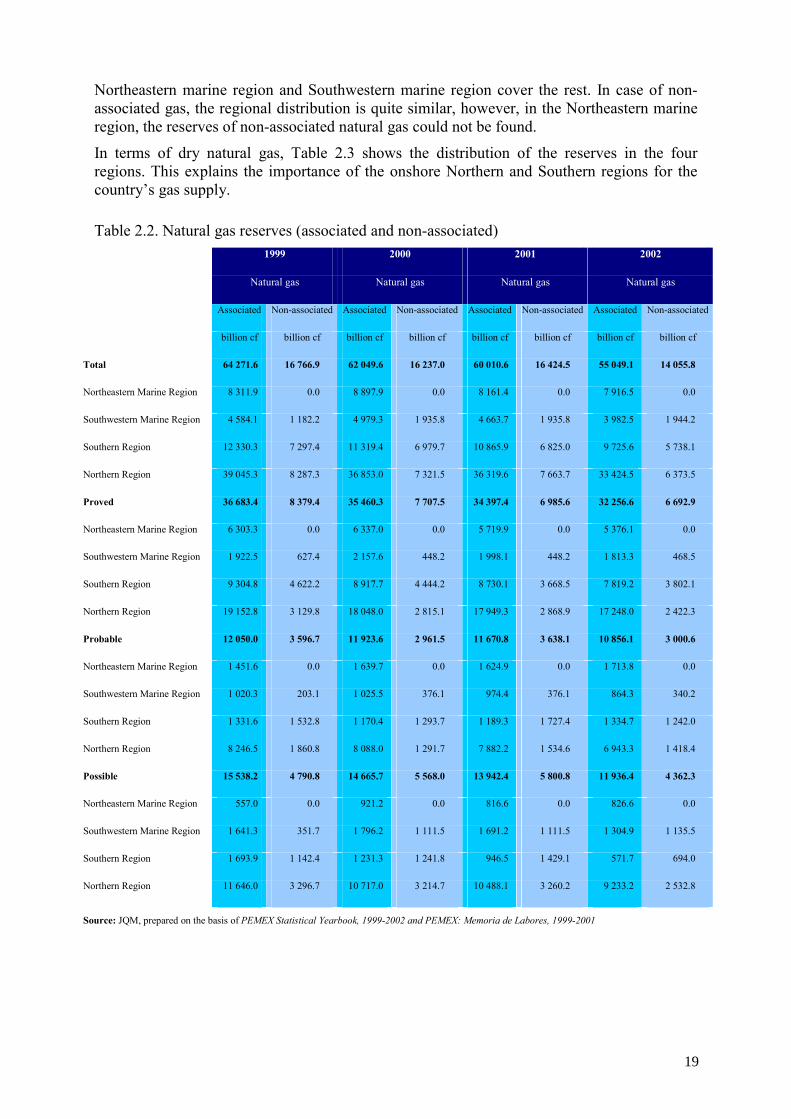
Northeastern marine region and Southwestern marine region cover the rest. In case of non-associated gas, the regional distribution is quite similar, however, in the Northeastern marine region, the reserves of non-associated natural gas could not be found.

In terms of dry natural gas, Table 2.3 shows the distribution of the reserves in the four regions. This explains the importance of the onshore Northern and Southern regions for the country’s gas supply.

Table 2.2. Natural gas reserves (associated and non-associated) 1999 2000 2001 2002

Natural gas Natural gas Natural gas Natural gas

Associated Non-associated Associated Non-associated Associated Non-associated Associated Non-associated

billion cf billion cf billion cf billion cf billion cf billion cf billion cf billion cf

Total 64 271.6 16 766.9 62 049.6 16 237.0 60 010.6 16 424.5 55 049.1 14 055.8


Southwestern Marine Region 4 584.1 1 182.2 4 979.3 1 935.8 4 663.7 1 935.8 3 982.5 1 944.2

Southern Region 12 330.3 7 297.4 11 319.4 6 979.7 10 865.9 6 825.0 9 725.6 5 738.1

Northern Region 39 045.3 8 287.3 36 853.0 7 321.5 36 319.6 7 663.7 33 424.5 6 373.5

Proved 36 683.4 8 379.4 35 460.3 7 707.5 34 397.4 6 985.6 32 256.6 6 692.9



Southern Region 9 304.8 4 622.2 8 917.7 4 444.2 8 730.1 3 668.5 7 819.2 3 802.1

Northern Region 19 152.8 3 129.8 18 048.0 2 815.1 17 949.3 2 868.9 17 248.0 2 422.3

Probable 12 050.0 3 596.7 11 923.6 2 961.5 11 670.8 3 638.1 10 856.1 3 000.6


Southwestern Marine Region 1 020.3 203.1 1 025.5 376.1 974.4 376.1 864.3 340.2

Southern Region 1 331.6 1 532.8 1 170.4 1 293.7 1 189.3 1 727.4 1 334.7 1 242.0

Northern Region 8 246.5 1 860.8 8 088.0 1 291.7 7 882.2 1 534.6 6 943.3 1 418.4

Possible 15 538.2 4 790.8 14 665.7 5 568.0 13 942.4 5 800.8 11 936.4 4 362.3

Northeastern Marine Region 557.0 0.0 921.2 0.0 816.6 0.0 826.6 0.0

Southwestern Marine Region 1 641.3 351.7 1 796.2 1 111.5 1 691.2 1 111.5 1 304.9 1 135.5

Southern Region 1 693.9 1 142.4 1 231.3 1 241.8 946.5 1 429.1 571.7 694.0

Northern Region 11 646.0 3 296.7 10 717.0 3 214.7 10 488.1 3 260.2 9 233.2 2 532.8

Source: JQM, prepared on the basis of PEMEX Statistical Yearbook, 1999-2002 and PEMEX: Memoria de Labores, 1999-2001

19

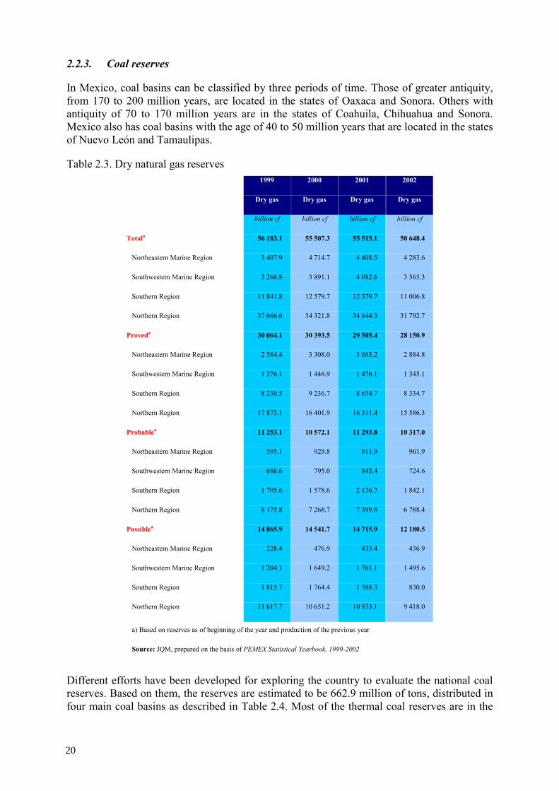
2.2.3. Coal reserves

In Mexico, coal basins can be classified by three periods of time. Those of greater antiquity, from 170 to 200 million years, are located in the states of Oaxaca and Sonora. Others with antiquity of 70 to 170 million years are in the states of Coahuila, Chihuahua and Sonora. Mexico also has coal basins with the age of 40 to 50 million years that are located in the states of Nuevo León and Tamaulipas.

Table 2.3. Dry natural gas reserves 1999 2000 2001 2002

Dry gas Dry gas Dry gas Dry gas

billion cf billion cf billion cf billion cf

Totala 56 183.1 55 507.3 55 515.1 50 648.4

Northeastern Marine Region 3 407.9 4 714.7 4 408.5 4 283.6

Southwestern Marine Region 3 266.8 3 891.1 4 082.6 3 565.3

Southern Region 11 841.8 12 579.7 12 379.7 11 006.8

Northern Region 37 666.6 34 321.8 34 644.3 31 792.7

Proveda 30 064.1 30 393.5 29 505.4 28 150.9

Northeastern Marine Region 2 584.4 3 308.0 3 063.2 2 884.8


Southern Region 8 230.5 9 236.7 8 654.7 8 334.7

Northern Region 17 873.1 16 401.9 16 311.4 15 586.3

Probablea 11 253.1 10 572.1 11 293.8 10 317.0

Northeastern Marine Region 595.1 929.8 911.9 961.9

Southwestern Marine Region 686.6 795.0 845.4 724.6

Southern Region 1 795.6 1 578.6 2 136.7 1 842.1

Northern Region 8 175.8 7 268.7 7 399.8 6 788.4

Possiblea 14 865.9 14 541.7 14 715.9 12 180.5

Northeastern Marine Region 228.4 476.9 433.4 436.9


Southern Region 1 815.7 1 764.4 1 588.3 830.0

Northern Region 11 617.7 10 651.2 10 933.1 9 418.0

a) Based on reserves as of beginning of the year and production of the previous year

Source: JQM, prepared on the basis of PEMEX Statistical Yearbook, 1999-2002

Different efforts have been developed for exploring the country to evaluate the national coal reserves. Based on them, the reserves are estimated to be 662.9 million of tons, distributed in four main coal basins as described in Table 2.4. Most of the thermal coal reserves are in the

20

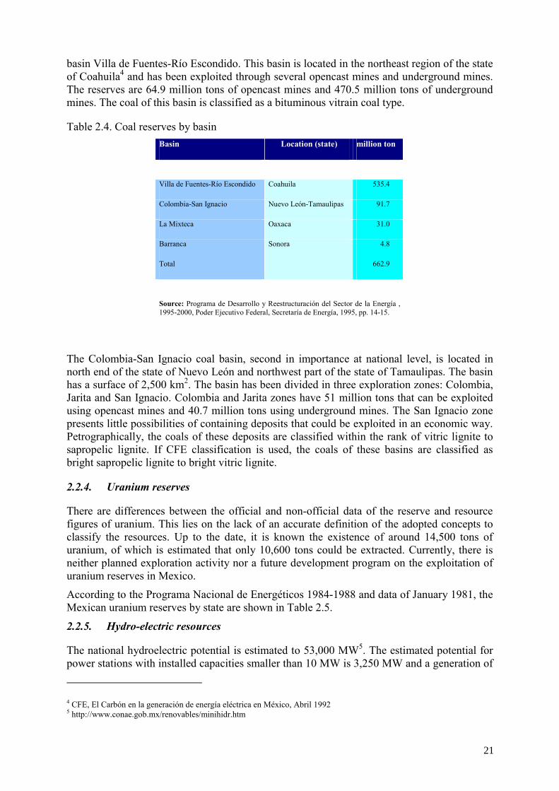
basin Villa de Fuentes-Río Escondido. This basin is located in the northeast region of the state of Coahuila4 and has been exploited through several opencast mines and underground mines. The reserves are 64.9 million tons of opencast mines and 470.5 million tons of underground mines. The coal of this basin is classified as a bituminous vitrain coal type.

Table 2.4. Coal reserves by basin Basin Location (state) million ton

Villa de Fuentes-Río Escondido Coahuila 535.4

Colombia-San Ignacio Nuevo León-Tamaulipas 91.7

La Mixteca Oaxaca 31.0

Barranca Sonora 4.8

Total 662.9

Source: Programa de Desarrollo y Reestructuración del Sector de la Energía , 1995-2000, Poder Ejecutivo Federal, Secretaría de Energía, 1995, pp. 14-15.

The Colombia-San Ignacio coal basin, second in importance at national level, is located in north end of the state of Nuevo León and northwest part of the state of Tamaulipas. The basin has a surface of 2,500 km2. The basin has been divided in three exploration zones: Colombia, Jarita and San Ignacio. Colombia and Jarita zones have 51 million tons that can be exploited using opencast mines and 40.7 million tons using underground mines. The San Ignacio zone presents little possibilities of containing deposits that could be exploited in an economic way. Petrographically, the coals of these deposits are classified within the rank of vitric lignite to sapropelic lignite. If CFE classification is used, the coals of these basins are classified as bright sapropelic lignite to bright vitric lignite.

2.2.4. Uranium reserves

There are differences between the official and non-official data of the reserve and resource figures of uranium. This lies on the lack of an accurate definition of the adopted concepts to classify the resources. Up to the date, it is known the existence of around 14,500 tons of uranium, of which is estimated that only 10,600 tons could be extracted. Currently, there is neither planned exploration activity nor a future development program on the exploitation of uranium reserves in Mexico.

According to the Programa Nacional de Energéticos 1984-1988 and data of January 1981, the Mexican uranium reserves by state are shown in Table 2.5.

2.2.5. Hydro-electric resources

The national hydroelectric potential is estimated to 53,000 MW5. The estimated potential for power stations with installed capacities smaller than 10 MW is 3,250 MW and a generation of

4 CFE, El Carbón en la generación de energía eléctrica en México, Abril 1992 5 http://www.conae.gob.mx/renovables/minihidr.htm

21

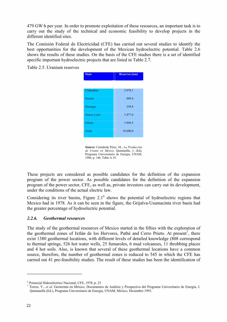
479 GW·h per year. In order to promote exploitation of these resources, an important task is to carry out the study of the technical and economic feasibility to develop projects in the different identified sites.

The Comisión Federal de Electricidad (CFE) has carried out several studies to identify the best opportunities for the development of the Mexican hydroelectric potential. Table 2.6 shows the results of these studies. On the basis of the CFE studies there is a set of identified specific important hydroelectric projects that are listed in Table 2.7.

Table 2.5. Uranium reserves State Reserves (ton)

Chihuahua 2 078.1

Sonora 889.6

Durango 258.8

Nuevo León 3 477.0

Others 3 896.5

Total 10 600.0

Source: Castañeda Pérez, M., La Producción de Uranio en México, Quintanilla, J. (Ed), Programa Universitario de Energía, UNAM, 1986, p. 146, Table A.19.

These projects are considered as possible candidates for the definition of the expansion program of the power sector. As possible candidates for the definition of the expansion program of the power sector, CFE, as well as, private investors can carry out its development, under the conditions of the actual electric law.

Considering its river basins, Figure 2.16 shows the potential of hydroelectric regions that Mexico had in 1978. As it can be seen in the figure, the Grijalva-Usumacinta river basin had the greater percentage of hydroelectric potential.

2.2.6. Geothermal resources

The study of the geothermal resources of Mexico started in the fifties with the exploration of the geothermal zones of Ixtlán de los Hervores, Pathé and Cerro Prieto. At present7, there exist 1380 geothermal locations, with different levels of detailed knowledge (808 correspond to thermal springs, 526 hot water wells, 25 fumaroles, 6 mud volcanoes, 11 throbbing places and 4 hot soils. Also, is known that several of these geothermal locations have a common source, therefore, the number of geothermal zones is reduced to 545 in which the CFE has carried out 41 pre-feasibility studies. The result of these studies has been the identification of

6 Potencial Hidroeléctrico Nacional, CFE, 1978, p. 23 7 Torres, V., et al, Geotermia en México, Documentos de Análisis y Prospectiva del Programa Universitario de Energía, J.

Quintanilla (Ed.), Programa Universitario de Energía, UNAM, México, Diciembre 1993.

22

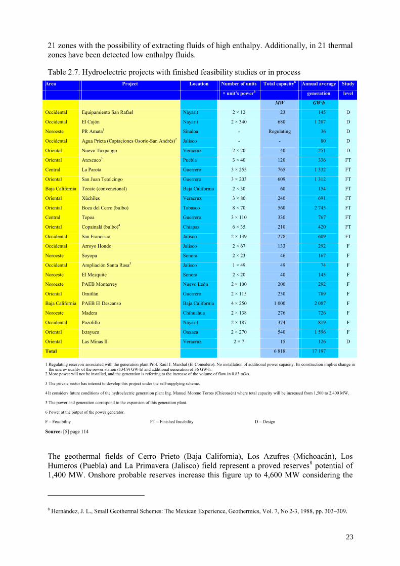
21 zones with the possibility of extracting fluids of high enthalpy. Additionally, in 21 thermal zones have been detected low enthalpy fluids.

Table 2.7. Hydroelectric projects with finished feasibility studies or in process Area Project Location Number of units Total capacity6 Annual average Study

× unit’s power6 generation level

MW GW·h

Occidental Equipamiento San Rafael Nayarit 2 × 12 23 145 D

Occidental El Cajón Nayarit 2 × 340 680 1 207 D

Noroeste PR Amata1 Sinaloa - Regulating 36 D

Occidental Agua Prieta (Captaciones Osorio-San Andrés)2 Jalisco - - 80 D

Oriental Nuevo Tuxpango Veracruz 2 × 20 40 251 D

Oriental Atexcaco3 Puebla 3 × 40 120 336 FT

Central La Parota Guerrero 3 × 255 765 1 332 FT

Oriental San Juan Tetelcingo Guerrero 3 × 203 609 1 312 FT

Baja California Tecate (convencional) Baja California 2 × 30 60 154 FT

Oriental Xúchiles Veracruz 3 × 80 240 691 FT

Oriental Boca del Cerro (bulbo) Tabasco 8 × 70 560 2 745 FT

Central Tepoa Guerrero 3 × 110 330 767 FT

Oriental Copainalá (bulbo)4 Chiapas 6 × 35 210 420 FT

Occidental San Francisco Jalisco 2 × 139 278 609 FT

Occidental Arroyo Hondo Jalisco 2 × 67 133 292 F

Noroeste Soyopa Sonora 2 × 23 46 167 F

Occidental Ampliación Santa Rosa5 Jalisco 1 × 49 49 74 F

Noroeste El Mezquite Sonora 2 × 20 40 145 F

Noroeste PAEB Monterrey Nuevo León 2 × 100 200 292 F

Oriental Omitlán Guerrero 2 × 115 230 789 F

Baja California PAEB El Descanso Baja California 4 × 250 1 000 2 087 F

Noroeste Madera Chihuahua 2 × 138 276 726 F

Occidental Pozolillo Nayarit 2 × 187 374 819 F

Oriental Ixtayuca Oaxaca 2 × 270 540 1 596 F

Oriental Las Minas II Veracruz 2 × 7 15 126 D

Total 6 818 17 197

1 Regulating reservoir associated with the generation plant Prof. Raúl J. Marshal (El Comedero). No installation of additional power capacity. Its construction implies change in the energy quality of the power station (134.9) GW·h) and additional generation of 36 GW·h.

2 More power will not be installed, and the generation is referring to the increase of the volume of flow in 0.83 m3/s.

3 The private sector has interest to develop this project under the self-supplying scheme.

4 It considers future conditions of the hydroelectric generation plant Ing. Manuel Moreno Torres (Chicoasén) where total capacity will be increased from 1,500 to 2,400 MW.

5 The power and generation correspond to the expansion of this generation plant.

6 Power at the output of the power generator.

F = Feasibility FT = Finished feasibility D = Design

Source: [5] page 114

The geothermal fields of Cerro Prieto (Baja California), Los Azufres (Michoacán), Los Humeros (Puebla) and La Primavera (Jalisco) field represent a proved reserves8 potential of 1,400 MW. Onshore probable reserves increase this figure up to 4,600 MW considering the

8 Hernández, J. L., Small Geothermal Schemes: The Mexican Experience, Geothermics, Vol. 7, No 2-3, 1988, pp. 303–309.

23

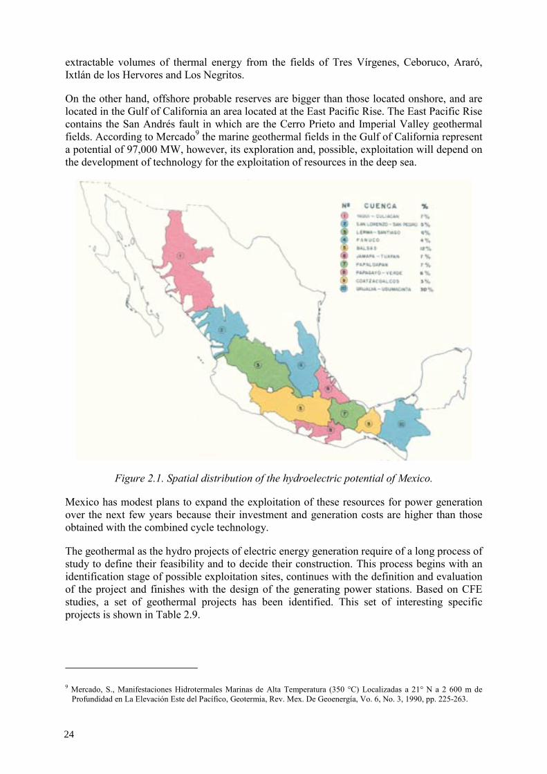
extractable volumes of thermal energy from the fields of Tres Vírgenes, Ceboruco, Araró, Ixtlán de los Hervores and Los Negritos.

On the other hand, offshore probable reserves are bigger than those located onshore, and are located in the Gulf of California an area located at the East Pacific Rise. The East Pacific Rise contains the San Andrés fault in which are the Cerro Prieto and Imperial Valley geothermal fields. According to Mercado9 the marine geothermal fields in the Gulf of California represent a potential of 97,000 MW, however, its exploration and, possible, exploitation will depend on the development of technology for the exploitation of resources in the deep sea.

Figure 2.1. Spatial distribution of the hydroelectric potential of Mexico.

Mexico has modest plans to expand the exploitation of these resources for power generation over the next few years because their investment and generation costs are higher than those obtained with the combined cycle technology.

The geothermal as the hydro projects of electric energy generation require of a long process of study to define their feasibility and to decide their construction. This process begins with an identification stage of possible exploitation sites, continues with the definition and evaluation of the project and finishes with the design of the generating power stations. Based on CFE studies, a set of geothermal projects has been identified. This set of interesting specific projects is shown in Table 2.9.

9 Mercado, S., Manifestaciones Hidrotermales Marinas de Alta Temperatura (350 °C) Localizadas a 21° N a 2 600 m de

Profundidad en La Elevación Este del Pacífico, Geotermia, Rev. Mex. De Geoenergía, Vo. 6, No. 3, 1990, pp. 225-263.

24

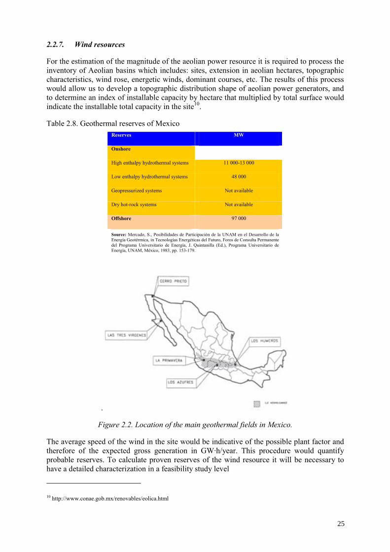
2.2.7. Wind resources

For the estimation of the magnitude of the aeolian power resource it is required to process the inventory of Aeolian basins which includes: sites, extension in aeolian hectares, topographic characteristics, wind rose, energetic winds, dominant courses, etc. The results of this process would allow us to develop a topographic distribution shape of aeolian power generators, and to determine an index of installable capacity by hectare that multiplied by total surface would indicate the installable total capacity in the site10.

Table 2.8. Geothermal reserves of Mexico Reserves MW

Onshore

High enthalpy hydrothermal systems 11 000-13 000

Low enthalpy hydrothermal systems 48 000

Geopressurized systems Not available

Dry hot-rock systems Not available

Offshore 97 000

Source: Mercado, S., Posibilidades de Participación de la UNAM en el Desarrollo de la Energía Geotérmica, in Tecnologías Energéticas del Futuro, Foros de Consulta Permanente del Programa Universitario de Energía, J. Quintanilla (Ed.), Programa Universitario de Energía, UNAM, México, 1983, pp. 153-179.

.

Figure 2.2. Location of the main geothermal fields in Mexico.

The average speed of the wind in the site would be indicative of the possible plant factor and therefore of the expected gross generation in GW·h/year. This procedure would quantify probable reserves. To calculate proven reserves of the wind resource it will be necessary to have a detailed characterization in a feasibility study level

10 http://www.conae.gob.mx/renovables/eolica.html

25

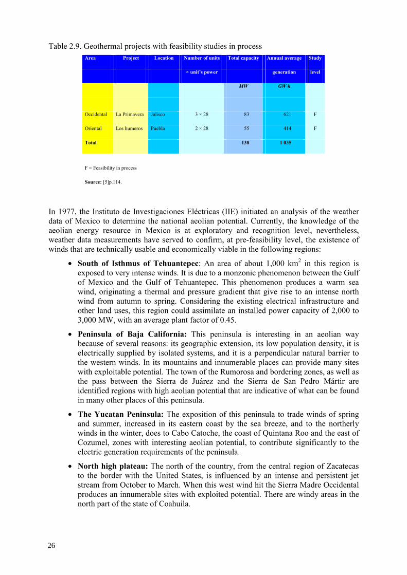
Table 2.9. Geothermal projects with feasibility studies in process Area Project Location Number of units Total capacity Annual average Study

× unit’s power generation level

MW GW·h

Occidental La Primavera Jalisco 3 × 28 83 621 F

Oriental Los humeros Puebla 2 × 28 55 414 F

Total 138 1 035

F = Feasibility in process

Source: [5]p.114.

In 1977, the Instituto de Investigaciones Eléctricas (IIE) initiated an analysis of the weather data of Mexico to determine the national aeolian potential. Currently, the knowledge of the aeolian energy resource in Mexico is at exploratory and recognition level, nevertheless, weather data measurements have served to confirm, at pre-feasibility level, the existence of winds that are technically usable and economically viable in the following regions:

• South of Isthmus of Tehuantepec: An area of about 1,000 km2 in this region is exposed to very intense winds. It is due to a monzonic phenomenon between the Gulf of Mexico and the Gulf of Tehuantepec. This phenomenon produces a warm sea wind, originating a thermal and pressure gradient that give rise to an intense north wind from autumn to spring. Considering the existing electrical infrastructure and other land uses, this region could assimilate an installed power capacity of 2,000 to 3,000 MW, with an average plant factor of 0.45.

• Peninsula of Baja California: This peninsula is interesting in an aeolian way because of several reasons: its geographic extension, its low population density, it is electrically supplied by isolated systems, and it is a perpendicular natural barrier to the western winds. In its mountains and innumerable places can provide many sites with exploitable potential. The town of the Rumorosa and bordering zones, as well as the pass between the Sierra de Juárez and the Sierra de San Pedro Mártir are identified regions with high aeolian potential that are indicative of what can be found in many other places of this peninsula.

• The Yucatan Peninsula: The exposition of this peninsula to trade winds of spring and summer, increased in its eastern coast by the sea breeze, and to the northerly winds in the winter, does to Cabo Catoche, the coast of Quintana Roo and the east of Cozumel, zones with interesting aeolian potential, to contribute significantly to the electric generation requirements of the peninsula.

• North high plateau: The north of the country, from the central region of Zacatecas to the border with the United States, is influenced by an intense and persistent jet stream from October to March. When this west wind hit the Sierra Madre Occidental produces an innumerable sites with exploited potential. There are windy areas in the north part of the state of Coahuila.

26

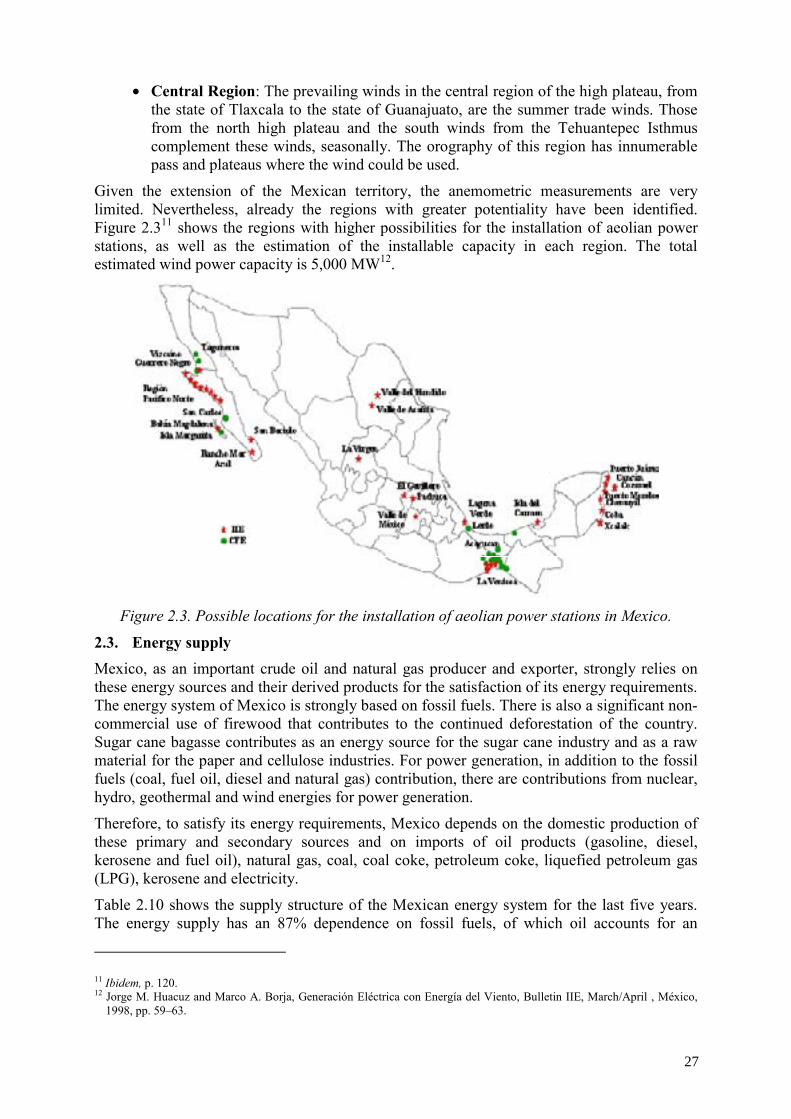
• Central Region: The prevailing winds in the central region of the high plateau, from the state of Tlaxcala to the state of Guanajuato, are the summer trade winds. Those from the north high plateau and the south winds from the Tehuantepec Isthmus complement these winds, seasonally. The orography of this region has innumerable pass and plateaus where the wind could be used.

Given the extension of the Mexican territory, the anemometric measurements are very limited. Nevertheless, already the regions with greater potentiality have been identified. Figure 2.311 shows the regions with higher possibilities for the installation of aeolian power stations, as well as the estimation of the installable capacity in each region. The total estimated wind power capacity is 5,000 MW12.

Figure 2.3. Possible locations for the installation of aeolian power stations in Mexico.

2.3. Energy supply Mexico, as an important crude oil and natural gas producer and exporter, strongly relies on these energy sources and their derived products for the satisfaction of its energy requirements. The energy system of Mexico is strongly based on fossil fuels. There is also a significant non-commercial use of firewood that contributes to the continued deforestation of the country. Sugar cane bagasse contributes as an energy source for the sugar cane industry and as a raw material for the paper and cellulose industries. For power generation, in addition to the fossil fuels (coal, fuel oil, diesel and natural gas) contribution, there are contributions from nuclear, hydro, geothermal and wind energies for power generation.

Therefore, to satisfy its energy requirements, Mexico depends on the domestic production of these primary and secondary sources and on imports of oil products (gasoline, diesel, kerosene and fuel oil), natural gas, coal, coal coke, petroleum coke, liquefied petroleum gas (LPG), kerosene and electricity.

Table 2.10 shows the supply structure of the Mexican energy system for the last five years. The energy supply has an 87% dependence on fossil fuels, of which oil accounts for an

11 Ibidem, p. 120. 12 Jorge M. Huacuz and Marco A. Borja, Generación Eléctrica con Energía del Viento, Bulletin IIE, March/April , México,

1998, pp. 59–63.

27

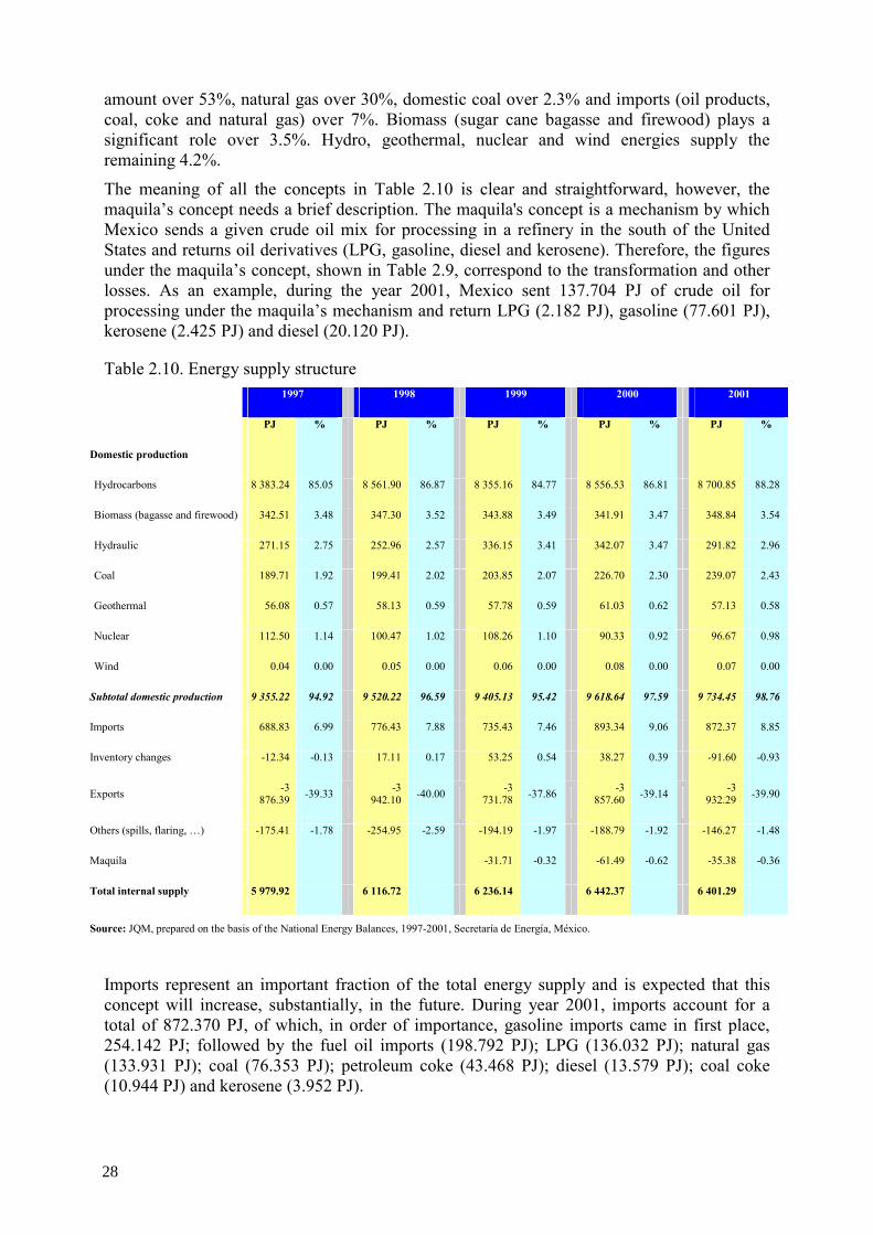
amount over 53%, natural gas over 30%, domestic coal over 2.3% and imports (oil products, coal, coke and natural gas) over 7%. Biomass (sugar cane bagasse and firewood) plays a significant role over 3.5%. Hydro, geothermal, nuclear and wind energies supply the remaining 4.2%.

The meaning of all the concepts in Table 2.10 is clear and straightforward, however, the maquila’s concept needs a brief description. The maquila's concept is a mechanism by which Mexico sends a given crude oil mix for processing in a refinery in the south of the United States and returns oil derivatives (LPG, gasoline, diesel and kerosene). Therefore, the figures under the maquila’s concept, shown in Table 2.9, correspond to the transformation and other losses. As an example, during the year 2001, Mexico sent 137.704 PJ of crude oil for processing under the maquila’s mechanism and return LPG (2.182 PJ), gasoline (77.601 PJ), kerosene (2.425 PJ) and diesel (20.120 PJ).

Table 2.10. Energy supply structure 1997 1998 1999 2000 2001

PJ % PJ % PJ % PJ % PJ %

Domestic production

Hydrocarbons 8 383.24 85.05 8 561.90 86.87 8 355.16 84.77 8 556.53 86.81 8 700.85 88.28

Biomass (bagasse and firewood) 342.51 3.48 347.30 3.52 343.88 3.49 341.91 3.47 348.84 3.54

Hydraulic 271.15 2.75 252.96 2.57 336.15 3.41 342.07 3.47 291.82 2.96

Coal 189.71 1.92 199.41 2.02 203.85 2.07 226.70 2.30 239.07 2.43

Geothermal 56.08 0.57 58.13 0.59 57.78 0.59 61.03 0.62 57.13 0.58

Nuclear 112.50 1.14 100.47 1.02 108.26 1.10 90.33 0.92 96.67 0.98

Wind 0.04 0.00 0.05 0.00 0.06 0.00 0.08 0.00 0.07 0.00

Subtotal domestic production 9 355.22 94.92 9 520.22 96.59 9 405.13 95.42 9 618.64 97.59 9 734.45 98.76

Imports 688.83 6.99 776.43 7.88 735.43 7.46 893.34 9.06 872.37 8.85

Inventory changes -12.34 -0.13 17.11 0.17 53.25 0.54 38.27 0.39 -91.60 -0.93

Exports -3 876.39 -39.33 -3

942.10 -40.00 -3 731.78 -37.86 -3

857.60 -39.14 -3 932.29 -39.90

Others (spills, flaring, …) -175.41 -1.78 -254.95 -2.59 -194.19 -1.97 -188.79 -1.92 -146.27 -1.48

Maquila -31.71 -0.32 -61.49 -0.62 -35.38 -0.36

Total internal supply 5 979.92 6 116.72 6 236.14 6 442.37 6 401.29

Source: JQM, prepared on the basis of the National Energy Balances, 1997-2001, Secretaría de Energía, México.

Imports represent an important fraction of the total energy supply and is expected that this concept will increase, substantially, in the future. During year 2001, imports account for a total of 872.370 PJ, of which, in order of importance, gasoline imports came in first place, 254.142 PJ; followed by the fuel oil imports (198.792 PJ); LPG (136.032 PJ); natural gas (133.931 PJ); coal (76.353 PJ); petroleum coke (43.468 PJ); diesel (13.579 PJ); coal coke (10.944 PJ) and kerosene (3.952 PJ).

28

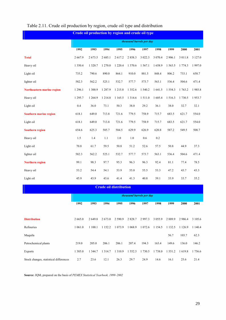
Table 2.11. Crude oil production by region, crude oil type and distribution Crude oil production by region and crude oil type

thousand barrels per day

1992 1993 1994 1995 1996 1997 1998 1999 2000 2001

Total 2 667.9 2 673.5 2 685.1 2 617.2 2 858.3 3 022.3 3 070.4 2 906.1 3 011.8 3 127.0

Heavy oil 1 350.4 1 320.7 1 270.0 1 220.4 1 370.6 1 567.1 1 658.9 1 563.5 1 774.3 1 997.0

Light oil 735.2 790.6 890.0 864.1 910.0 881.5 848.4 806.2 733.1 658.7

lighter oil 582.3 562.2 525.1 532.7 577.7 573.7 563.1 536.4 504.6 471.4

Northeastern marine region 1 296.1 1 300.9 1 287.9 1 215.8 1 352.6 1 540.2 1 641.5 1 554.3 1 763.2 1 985.8

Heavy oil 1 295.7 1 264.9 1 214.8 1 165.5 1 314.6 1 511.0 1 605.4 1 516.3 1 730.5 1 953.7

Light oil 0.4 36.0 73.1 50.3 38.0 29.2 36.1 38.0 32.7 32.1

Southern marine region 618.1 649.0 713.8 721.6 779.5 758.9 715.7 683.5 621.7 554.0

Light oil 618.1 649.0 713.8 721.6 779.5 758.9 715.7 683.5 621.7 554.0

Southern region 654.6 625.3 585.7 584.5 629.9 626.9 620.8 587.2 549.5 508.7

Heavy oil 1.5 1.4 1.1 1.0 1.0 0.6 0.2

Light oil 70.8 61.7 59.5 50.8 51.2 52.6 57.5 50.8 44.9 37.3

lighter oil 582.3 562.2 525.1 532.7 577.7 573.7 563.1 536.4 504.6 471.4

Northern region 99.1 98.3 97.7 95.3 96.3 96.3 92.4 81.1 77.4 78.5

Heavy oil 53.2 54.4 54.1 53.9 55.0 55.5 53.3 47.2 43.7 43.3

Light oil 45.9 43.9 43.6 41.4 41.3 40.8 39.1 33.9 33.7 35.2

Crude oil distribution

thousand barrels per day

1992 1993 1994 1995 1996 1997 1998 1999 2000 2001

Distribution 2 665.0 2 649.8 2 673.0 2 590.9 2 828.7 2 997.3 3 055.9 2 889.9 2 986.4 3 105.6

Refineries 1 061.0 1 100.1 1 152.2 1 073.9 1 068.9 1 072.6 1 154.5 1 132.5 1 126.9 1 140.4

Maquila 56.7 103.7 62.3

Petrochemical plants 219.0 205.0 206.1 206.1 207.4 194.3 163.4 149.6 136.0 146.2

Exports 1 385.0 1 344.7 1 314.7 1 310.9 1 552.3 1 730.5 1 738.0 1 551.2 1 619.8 1 756.6

Stock changes, statistical differences 2.7 23.6 12.1 26.3 29.7 24.9 14.6 16.1 25.6 21.4

Source: JQM, prepared on the basis of PEMEX Statistical Yearbook, 1999–2002

29

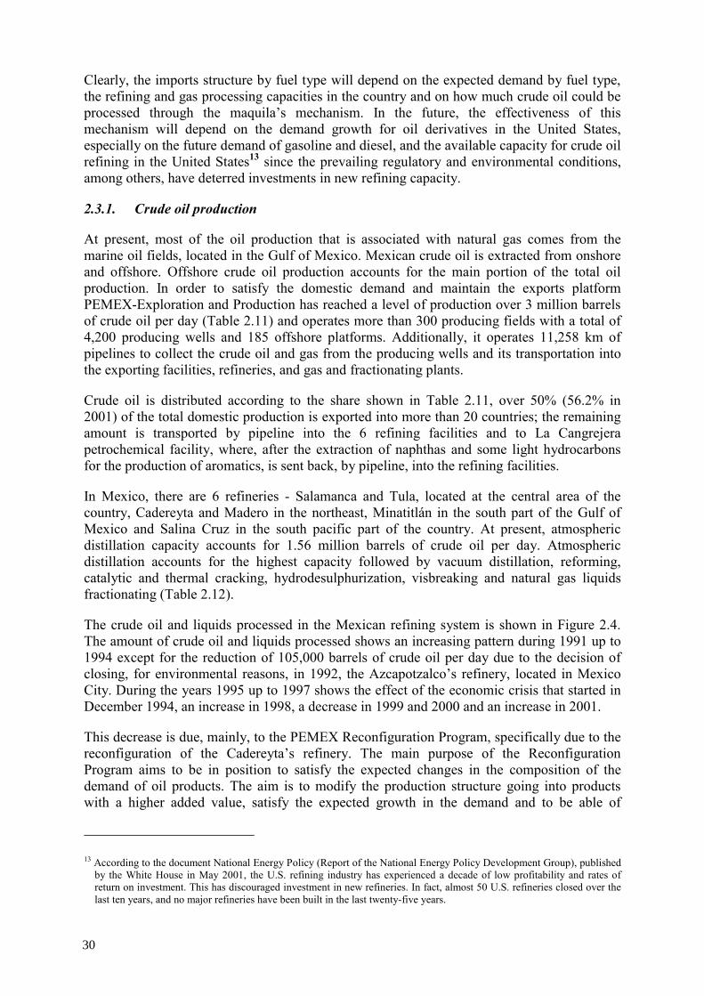
Clearly, the imports structure by fuel type will depend on the expected demand by fuel type, the refining and gas processing capacities in the country and on how much crude oil could be processed through the maquila’s mechanism. In the future, the effectiveness of this mechanism will depend on the demand growth for oil derivatives in the United States, especially on the future demand of gasoline and diesel, and the available capacity for crude oil refining in the United States13 since the prevailing regulatory and environmental conditions, among others, have deterred investments in new refining capacity.

2.3.1. Crude oil production

At present, most of the oil production that is associated with natural gas comes from the marine oil fields, located in the Gulf of Mexico. Mexican crude oil is extracted from onshore and offshore. Offshore crude oil production accounts for the main portion of the total oil production. In order to satisfy the domestic demand and maintain the exports platform PEMEX-Exploration and Production has reached a level of production over 3 million barrels of crude oil per day (Table 2.11) and operates more than 300 producing fields with a total of 4,200 producing wells and 185 offshore platforms. Additionally, it operates 11,258 km of pipelines to collect the crude oil and gas from the producing wells and its transportation into the exporting facilities, refineries, and gas and fractionating plants.

Crude oil is distributed according to the share shown in Table 2.11, over 50% (56.2% in 2001) of the total domestic production is exported into more than 20 countries; the remaining amount is transported by pipeline into the 6 refining facilities and to La Cangrejera petrochemical facility, where, after the extraction of naphthas and some light hydrocarbons for the production of aromatics, is sent back, by pipeline, into the refining facilities.

In Mexico, there are 6 refineries - Salamanca and Tula, located at the central area of the country, Cadereyta and Madero in the northeast, Minatitlán in the south part of the Gulf of Mexico and Salina Cruz in the south pacific part of the country. At present, atmospheric distillation capacity accounts for 1.56 million barrels of crude oil per day. Atmospheric distillation accounts for the highest capacity followed by vacuum distillation, reforming, catalytic and thermal cracking, hydrodesulphurization, visbreaking and natural gas liquids fractionating (Table 2.12).

The crude oil and liquids processed in the Mexican refining system is shown in Figure 2.4. The amount of crude oil and liquids processed shows an increasing pattern during 1991 up to 1994 except for the reduction of 105,000 barrels of crude oil per day due to the decision of closing, for environmental reasons, in 1992, the Azcapotzalco’s refinery, located in Mexico City. During the years 1995 up to 1997 shows the effect of the economic crisis that started in December 1994, an increase in 1998, a decrease in 1999 and 2000 and an increase in 2001.

This decrease is due, mainly, to the PEMEX Reconfiguration Program, specifically due to the reconfiguration of the Cadereyta’s refinery. The main purpose of the Reconfiguration Program aims to be in position to satisfy the expected changes in the composition of the demand of oil products. The aim is to modify the production structure going into products with a higher added value, satisfy the expected growth in the demand and to be able of

13 According to the document National Energy Policy (Report of the National Energy Policy Development Group), published

by the White House in May 2001, the U.S. refining industry has experienced a decade of low profitability and rates of return on investment. This has discouraged investment in new refineries. In fact, almost 50 U.S. refineries closed over the last ten years, and no major refineries have been built in the last twenty-five years.

30

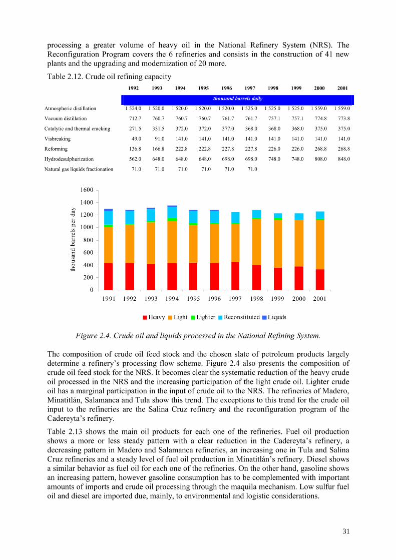
processing a greater volume of heavy oil in the National Refinery System (NRS). The Reconfiguration Program covers the 6 refineries and consists in the construction of 41 new plants and the upgrading and modernization of 20 more.

Table 2.12. Crude oil refining capacity 1992 1993 1994 1995 1996 1997 1998 1999 2000 2001

thousand barrels daily

Atmospheric distillation 1 524.0 1 520.0 1 520.0 1 520.0 1 520.0 1 525.0 1 525.0 1 525.0 1 559.0 1 559.0

Vacuum distillation 712.7 760.7 760.7 760.7 761.7 761.7 757.1 757.1 774.8 773.8

Catalytic and thermal cracking 271.5 331.5 372.0 372.0 377.0 368.0 368.0 368.0 375.0 375.0

Visbreaking 49.0 91.0 141.0 141.0 141.0 141.0 141.0 141.0 141.0 141.0

Reforming 136.8 166.8 222.8 222.8 227.8 227.8 226.0 226.0 268.8 268.8

Hydrodesulphurization 562.0 648.0 648.0 648.0 698.0 698.0 748.0 748.0 808.0 848.0

Natural gas liquids fractionation 71.0 71.0 71.0 71.0 71.0 71.0

0

200

400

600

800

1000

1200

1400

1600

1991 1992 1993 1994 1995 1996 1997 1998 1999 2000 2001

thou

sand

bar

rels

per d

ay

Heavy Light Lighter Reconstituted Liquids

Figure 2.4. Crude oil and liquids processed in the National Refining System.

The composition of crude oil feed stock and the chosen slate of petroleum products largely determine a refinery’s processing flow scheme. Figure 2.4 also presents the composition of crude oil feed stock for the NRS. It becomes clear the systematic reduction of the heavy crude oil processed in the NRS and the increasing participation of the light crude oil. Lighter crude oil has a marginal participation in the input of crude oil to the NRS. The refineries of Madero, Minatitlán, Salamanca and Tula show this trend. The exceptions to this trend for the crude oil input to the refineries are the Salina Cruz refinery and the reconfiguration program of the Cadereyta’s refinery.

Table 2.13 shows the main oil products for each one of the refineries. Fuel oil production shows a more or less steady pattern with a clear reduction in the Cadereyta’s refinery, a decreasing pattern in Madero and Salamanca refineries, an increasing one in Tula and Salina Cruz refineries and a steady level of fuel oil production in Minatitlán’s refinery. Diesel shows a similar behavior as fuel oil for each one of the refineries. On the other hand, gasoline shows an increasing pattern, however gasoline consumption has to be complemented with important amounts of imports and crude oil processing through the maquila mechanism. Low sulfur fuel oil and diesel are imported due, mainly, to environmental and logistic considerations.

31

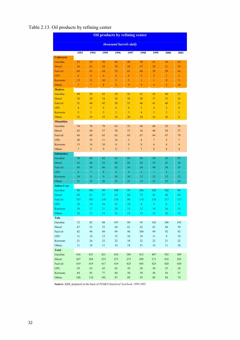
Table 2.13. Oil products by refining center Oil products by refining center

thousand barrels daily

1993 1994 1995 1996 1997 1998 1999 2000 2001 Cadereyta Gasoline 55 54 50 46 48 50 41 34 64 Diesel 36 42 39 39 44 47 28 31 59 Fuel oil 68 65 64 55 61 60 38 50 66 LPG 6 6 6 6 6 5 2 1 2 Kerosene 15 15 10 5 5 1 1 0 3 Others 5 7 8 8 9 9 4 4 10 Madero Gasoline 49 50 43 39 41 41 43 40 23 Diesel 38 38 34 30 30 30 37 35 26 Fuel oil 51 44 45 50 51 46 41 40 32 LPG 4 5 6 6 6 3 4 2 0 Kerosene 5 5 5 3 3 4 3 3 1 Others 32 34 35 18 20 24 26 20 8 Minatitlán Gasoline 74 76 79 63 53 64 60 55 56 Diesel 43 44 37 38 37 36 40 38 37 Fuel oil 66 68 63 62 65 67 64 67 70 LPG 20 19 11 16 3 4 7 5 7 Kerosene 15 14 10 8 9 8 6 4 4 Others 7 9 9 11 7 7 8 8 8 Salamanca Gasoline 70 69 62 61 63 56 59 55 55 Diesel 43 46 35 40 43 42 39 41 38 Fuel oil 45 39 46 43 54 54 49 54 55 LPG 8 7 8 6 4 2 1 3 3 Kerosene 10 8 9 10 10 12 12 12 12 Others 31 33 26 23 21 19 23 25 24 Salina Cruz Gasoline 96 100 99 100 95 106 102 102 89 Diesel 60 61 57 62 60 72 65 60 64 Fuel oil 107 105 110 110 98 118 134 117 115 LPG 10 14 16 13 10 4 5 6 6 Kerosene 18 17 21 20 13 12 14 16 15 Others 22 13 13 13 13 15 12 16 14 Tula Gasoline 72 82 88 107 89 95 102 106 102 Diesel 47 53 53 64 61 62 62 60 59 Fuel oil 82 98 89 99 96 100 99 92 92 LPG 11 14 15 15 10 10 11 8 10 Kerosene 21 26 22 22 18 22 22 21 22 Others 11 14 11 14 19 21 16 11 10

Total Gasoline 416 431 421 416 389 412 407 392 389 Diesel 267 284 255 273 275 289 271 265 283 Fuel oil 419 419 417 419 425 445 425 420 430 LPG 59 65 62 62 39 28 30 25 28 Kerosene 84 85 77 68 58 59 58 56 57 Others 108 110 102 87 89 95 89 84 74

Source: JQM, prepared on the basis of PEMEX Statistical Yearbook, 1999-2002

32

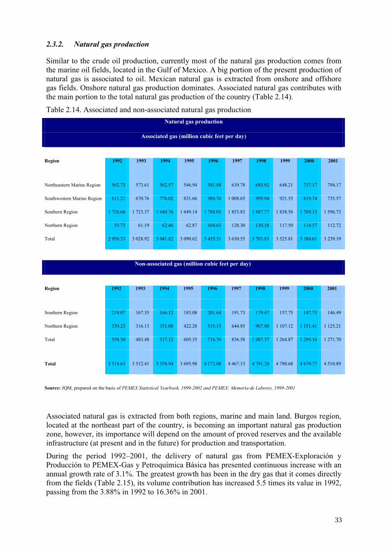
2.3.2. Natural gas production

Similar to the crude oil production, currently most of the natural gas production comes from the marine oil fields, located in the Gulf of Mexico. A big portion of the present production of natural gas is associated to oil. Mexican natural gas is extracted from onshore and offshore gas fields. Onshore natural gas production dominates. Associated natural gas contributes with the main portion to the total natural gas production of the country (Table 2.14).

Table 2.14. Associated and non-associated natural gas production Natural gas production

Associated gas (million cubic feet per day)

Region 1992 1993 1994 1995 1996 1997 1998 1999 2000 2001

Northeastern Marine Region 562.73 573.61 562.57 546.94 581.88 639.78 685.92 648.21 737.17 794.17

Southwestern Marine Region 611.21 670.76 776.02 831.66 980.76 1 008.65 999.94 921.55 819.74 735.57

Southern Region 1 726.66 1 723.37 1 640.76 1 649.14 1 788.05 1 853.83 1 887.77 1 838.56 1 709.13 1 596.73

Northern Region 55.73 61.19 62.46 62.87 104.63 128.30 130.18 117.50 114.57 112.72

Total 2 956.33 3 028.92 3 041.82 3 090.62 3 455.31 3 630.55 3 703.83 3 525.81 3 380.61 3 239.19

Non-associated gas (million cubic feet per day)

Region 1992 1993 1994 1995 1996 1997 1998 1999 2000 2001

Southern Region 219.07 167.35 166.12 183.08 201.64 191.73 179.47 157.75 147.75 146.49

Northern Region 339.23 316.13 351.00 422.28 515.13 644.85 907.90 1 107.12 1 151.41 1 125.21

Total 558.30 483.48 517.12 605.35 716.76 836.58 1 087.37 1 264.87 1 299.16 1 271.70

Total 3 514.63 3 512.41 3 558.94 3 695.98 4 172.08 4 467.13 4 791.20 4 790.68 4 679.77 4 510.89


Associated natural gas is extracted from both regions, marine and main land. Burgos region, located at the northeast part of the country, is becoming an important natural gas production zone, however, its importance will depend on the amount of proved reserves and the available infrastructure (at present and in the future) for production and transportation.

During the period 1992–2001, the delivery of natural gas from PEMEX-Exploración y Producción to PEMEX-Gas y Petroquímica Básica has presented continuous increase with an annual growth rate of 3.1%. The greatest growth has been in the dry gas that it comes directly from the fields (Table 2.15), its volume contribution has increased 5.5 times its value in 1992, passing from the 3.88% in 1992 to 16.36% in 2001.

33

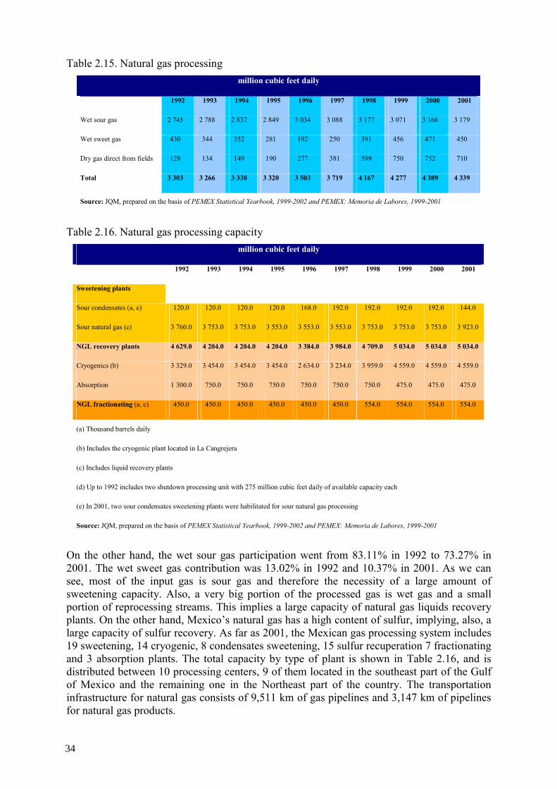
Table 2.15. Natural gas processing million cubic feet daily

1992 1993 1994 1995 1996 1997 1998 1999 2000 2001

Wet sour gas 2 745 2 788 2 837 2 849 3 034 3 088 3 177 3 071 3 166 3 179

Wet sweet gas 430 344 352 281 192 250 391 456 471 450

Dry gas direct from fields 128 134 149 190 277 381 599 750 752 710

Total 3 303 3 266 3 338 3 320 3 503 3 719 4 167 4 277 4 389 4 339


Table 2.16. Natural gas processing capacity

million cubic feet daily

1992 1993 1994 1995 1996 1997 1998 1999 2000 2001

Sweetening plants

Sour condensates (a, e) 120.0 120.0 120.0 120.0 168.0 192.0 192.0 192.0 192.0 144.0

Sour natural gas (e) 3 760.0 3 753.0 3 753.0 3 553.0 3 553.0 3 553.0 3 753.0 3 753.0 3 753.0 3 923.0

NGL recovery plants 4 629.0 4 204.0 4 204.0 4 204.0 3 384.0 3 984.0 4 709.0 5 034.0 5 034.0 5 034.0

Cryogenics (b) 3 329.0 3 454.0 3 454.0 3 454.0 2 634.0 3 234.0 3 959.0 4 559.0 4 559.0 4 559.0

Absorption 1 300.0 750.0 750.0 750.0 750.0 750.0 750.0 475.0 475.0 475.0

NGL fractionating (a, c) 450.0 450.0 450.0 450.0 450.0 450.0 554.0 554.0 554.0 554.0

(a) Thousand barrels daily

(b) Includes the cryogenic plant located in La Cangrejera

(c) Includes liquid recovery plants

(d) Up to 1992 includes two shutdown processing unit with 275 million cubic feet daily of available capacity each

(e) In 2001, two sour condensates sweetening plants were habilitated for sour natural gas processing


On the other hand, the wet sour gas participation went from 83.11% in 1992 to 73.27% in 2001. The wet sweet gas contribution was 13.02% in 1992 and 10.37% in 2001. As we can see, most of the input gas is sour gas and therefore the necessity of a large amount of sweetening capacity. Also, a very big portion of the processed gas is wet gas and a small portion of reprocessing streams. This implies a large capacity of natural gas liquids recovery plants. On the other hand, Mexico’s natural gas has a high content of sulfur, implying, also, a large capacity of sulfur recovery. As far as 2001, the Mexican gas processing system includes 19 sweetening, 14 cryogenic, 8 condensates sweetening, 15 sulfur recuperation 7 fractionating and 3 absorption plants. The total capacity by type of plant is shown in Table 2.16, and is distributed between 10 processing centers, 9 of them located in the southeast part of the Gulf of Mexico and the remaining one in the Northeast part of the country. The transportation infrastructure for natural gas consists of 9,511 km of gas pipelines and 3,147 km of pipelines for natural gas products.

34

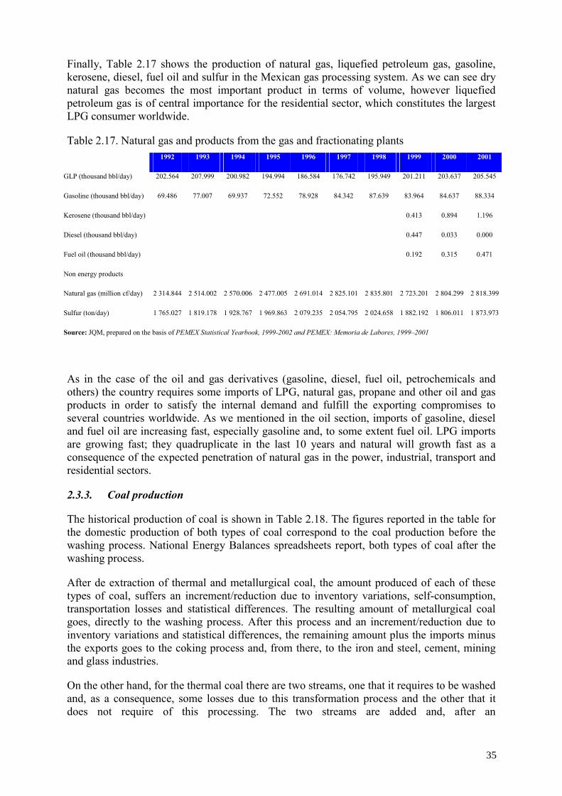
Finally, Table 2.17 shows the production of natural gas, liquefied petroleum gas, gasoline, kerosene, diesel, fuel oil and sulfur in the Mexican gas processing system. As we can see dry natural gas becomes the most important product in terms of volume, however liquefied petroleum gas is of central importance for the residential sector, which constitutes the largest LPG consumer worldwide.

Table 2.17. Natural gas and products from the gas and fractionating plants 1992 1993 1994 1995 1996 1997 1998 1999 2000 2001

GLP (thousand bbl/day) 202.564 207.999 200.982 194.994 186.584 176.742 195.949 201.211 203.637 205.545

Gasoline (thousand bbl/day) 69.486 77.007 69.937 72.552 78.928 84.342 87.639 83.964 84.637 88.334

Kerosene (thousand bbl/day) 0.413 0.894 1.196

Diesel (thousand bbl/day) 0.447 0.033 0.000

Fuel oil (thousand bbl/day) 0.192 0.315 0.471

Non energy products

Natural gas (million cf/day) 2 314.844 2 514.002 2 570.006 2 477.005 2 691.014 2 825.101 2 835.801 2 723.201 2 804.299 2 818.399

Sulfur (ton/day) 1 765.027 1 819.178 1 928.767 1 969.863 2 079.235 2 054.795 2 024.658 1 882.192 1 806.011 1 873.973

Source: JQM, prepared on the basis of PEMEX Statistical Yearbook, 1999-2002 and PEMEX: Memoria de Labores, 1999–2001

As in the case of the oil and gas derivatives (gasoline, diesel, fuel oil, petrochemicals and others) the country requires some imports of LPG, natural gas, propane and other oil and gas products in order to satisfy the internal demand and fulfill the exporting compromises to several countries worldwide. As we mentioned in the oil section, imports of gasoline, diesel and fuel oil are increasing fast, especially gasoline and, to some extent fuel oil. LPG imports are growing fast; they quadruplicate in the last 10 years and natural will growth fast as a consequence of the expected penetration of natural gas in the power, industrial, transport and residential sectors.

2.3.3. Coal production

The historical production of coal is shown in Table 2.18. The figures reported in the table for the domestic production of both types of coal correspond to the coal production before the washing process. National Energy Balances spreadsheets report, both types of coal after the washing process.

After de extraction of thermal and metallurgical coal, the amount produced of each of these types of coal, suffers an increment/reduction due to inventory variations, self-consumption, transportation losses and statistical differences. The resulting amount of metallurgical coal goes, directly to the washing process. After this process and an increment/reduction due to inventory variations and statistical differences, the remaining amount plus the imports minus the exports goes to the coking process and, from there, to the iron and steel, cement, mining and glass industries.

On the other hand, for the thermal coal there are two streams, one that it requires to be washed and, as a consequence, some losses due to this transformation process and the other that it does not require of this processing. The two streams are added and, after an

35

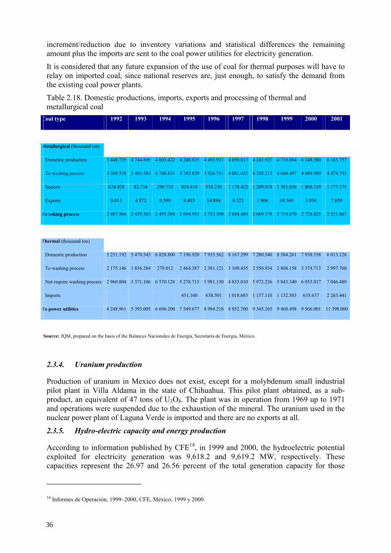
increment/reduction due to inventory variations and statistical differences the remaining amount plus the imports are sent to the coal power utilities for electricity generation.

It is considered that any future expansion of the use of coal for thermal purposes will have to relay on imported coal, since national reserves are, just enough, to satisfy the demand from the existing coal power plants.

Table 2.18. Domestic productions, imports, exports and processing of thermal and metallurgical coal

Coal type 1992 1993 1994 1995 1996 1997 1998 1999 2000 2001

Metallurgical (thousand ton)

Domestic production 3 448.735 4 744.809 4 603.422 4 248.835 4 493.931 4 050.813 4 243.927 4 718.084 6 348.580 6 163.757

To washing process 3 268.528 3 483.583 4 788.833 3 745.829 3 926.751 4 061.432 4 358.215 4 668.697 4 689.989 4 474.751

Imports 634.029 82.734 290.733 819.810 938.230 1 178.422 1 209.918 1 381.656 1 800.339 1 177.175

Exports 0.013 4.972 0.599 0.485 14.894 0.323 1.906 69.369 3.956 7.659

To coking process 2 487.566 2 439.363 2 493.380 2 694.953 2 752.509 2 684.489 2 689.179 2 719.670 2 728.825 2 521.867

Thermal (thousand ton)

Domestic production 5 251.192 5 470.543 6 828.800 7 196.920 7 935.562 8 167.299 7 280.540 8 584.261 7 938.558 6 013.126

To washing process 2 175.146 1 836.284 279.012 2 464.387 2 381.121 3 109.455 2 550.934 2 808.158 3 374.713 2 997.760

Not require washing process 2 960.804 3 371.106 6 570.128 5 278.715 5 981.130 4 835.010 5 972.236 5 843.340 6 053.017 7 046.489

Imports 451.160 638.501 1 018.683 1 157.110 1 132.503 635.637 2 263.441

To power utilities 4 248.961 5 393.005 6 696.200 7 549.677 8 984.218 8 852.700 9 345.265 9 468.498 9 566.001 11 398.000

Source: JQM, prepared on the basis of the Balances Nacionales de Energía, Secretaría de Energía, México.

2.3.4. Uranium production

Production of uranium in Mexico does not exist, except for a molybdenum small industrial pilot plant in Villa Aldama in the state of Chihuahua. This pilot plant obtained, as a sub-product, an equivalent of 47 tons of U3O8. The plant was in operation from 1969 up to 1971 and operations were suspended due to the exhaustion of the mineral. The uranium used in the nuclear power plant of Laguna Verde is imported and there are no exports at all.

2.3.5. Hydro-electric capacity and energy production

According to information published by CFE14, in 1999 and 2000, the hydroelectric potential exploited for electricity generation was 9,618.2 and 9,619.2 MW, respectively. These capacities represent the 26.97 and 26.56 percent of the total generation capacity for those

14 Informes de Operación, 1999–2000, CFE, México, 1999 y 2000.

36

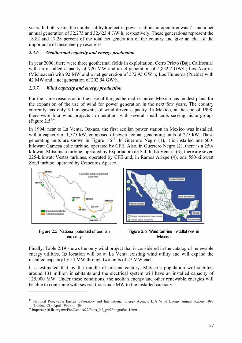
years. In both years, the number of hydroelectric power stations in operation was 71 and a net annual generation of 32,275 and 32,623.4 GW·h, respectively. These generations represent the 18.82 and 17.28 percent of the total net generation of the country and give an idea of the importance of these energy resources.

2.3.6. Geothermal capacity and energy production

In year 2000, there were three geothermal fields in exploitation, Cerro Prieto (Baja California) with an installed capacity of 720 MW and a net generation of 4,852.7 GW·h; Los Azufres (Michoacán) with 92 MW and a net generation of 572.95 GW·h; Los Humeros (Puebla) with 42 MW and a net generation of 202.94 GW·h.

2.3.7. Wind capacity and energy production

For the same reasons as in the case of the geothermal resource, Mexico has modest plans for the expansion of the use of wind for power generation in the next few years. The country currently has only 3.1 megawatts of wind-driven capacity. In Mexico, at the end of 1998, there were four wind projects in operation, with several small units serving niche groups (Figure 2.515).

In 1994, near to La Venta, Oaxaca, the first aeolian power station in Mexico was installed, with a capacity of 1,575 kW, composed of seven aeolian generating units of 225 kW. These generating units are shown in Figure 1.616. In Guerrero Negro (1), it is installed one 600-kilowatt Gamesa eolic turbine, operated by CFE. Also, in Guerrero Negro (2), there is a 250-kilowatt Mitsubishi turbine, operated by Exportadora de Sal. In La Venta I (3), there are seven 225-kilowatt Vestas turbines, operated by CFE and, in Ramos Arizpe (4), one 550-kilowatt Zond turbine, operated by Cementos Apasco.

Figure 2.5 National potential of aeolian capacity

Figure 2.6 Wind turbine installations in Mexico

Figure 2.5 National potential of aeolian capacity



Finally, Table 2.19 shows the only wind project that is considered in the catalog of renewable energy utilities. Its location will be at La Venta existing wind utility and will expand the installed capacity by 54 MW through two units of 27 MW each.

It is estimated that by the middle of present century, Mexico’s population will stabilize around 131 million inhabitants and the electrical system will have an installed capacity of 125,000 MW. Under these conditions, the aeolian energy and other renewable energies will be able to contribute with several thousands MW to the installed capacity. 15 National Renewable Energy Laboratory and International Energy Agency, IEA Wind Energy Annual Report 1998

(Golden, CO, April 1999), p. 109. 16 http://axp16.iie.org.mx/FnoC/eolica22/fotos_inf_graf/fotografia4.1.htm

37

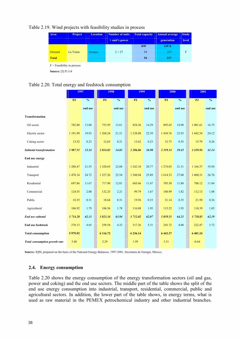
Table 2.19. Wind projects with feasibility studies in process Area Project Location Number of units Total capacity Annual average Study

× unit’s power generation level

MW GW·h

Oriental La Venta Oaxaca 2 × 27 54 237 F

Total 54 237

F = Feasibility in process

Source: [5] P:114

Table 2.20. Total energy and feedstock consumption 1997 1998 1999 2000 2001


end use end use end use end use end use

Transformation

Oil sector 782.00 13.08 753.95 12.61 854.36 14.29 895.65 14.98 1 001.61 16.75

Electric sector 1 191.99 19.93 1 268.24 21.21 1 338.88 22.39 1 430.76 23.93 1 442.54 24.12

Coking sector 13.52 0.23 12.65 0.21 13.62 0.23 32.73 0.55 15.79 0.26

Subtotal transformation 1 987.51 33.24 2 034.83 34.03 2 206.86 36.90 2 359.14 39.45 2 459.94 41.14

End use energy

Industrial 1 288.47 21.55 1 320.65 22.08 1 242.10 20.77 1 274.03 21.31 1 166.37 19.50

Transport 1 478.14 24.72 1 527.26 25.54 1 548.04 25.89 1 614.33 27.00 1 600.31 26.76

Residential 697.86 11.67 717.98 12.01 685.66 11.47 705.50 11.80 708.12 11.84

Commercial 124.55 2.08 132.25 2.21 99.79 1.67 108.99 1.82 112.13 1.88

Public 18.35 0.31 18.64 0.31 19.56 0.33 21.14 0.35 21.50 0.36

Agricultural 106.92 1.79 106.56 1.78 116.88 1.95 115.52 1.93 110.39 1.85

End use subtotal 3 714.28 62.11 3 823.34 63.94 3 712.02 62.07 3 839.51 64.21 3 718.83 62.19

End use feedstock 278.13 4.65 258.54 4.32 317.26 5.31 243.72 4.08 222.47 3.72

Total consumption 5 979.92 6 116.72 6 236.14 6 442.37 6 401.24

Total consumption growth rate 3.48 2.29 1.95 3.31 -0.64

Source: JQM, prepared on the basis of the National Energy Balances, 1997-2001, Secretaría de Energía, México.

2.4. Energy consumption

Table 2.20 shows the energy consumption of the energy transformation sectors (oil and gas, power and coking) and the end use sectors. The middle part of the table shows the split of the end use energy consumption into industrial, transport, residential, commercial, public and agricultural sectors. In addition, the lower part of the table shows, in energy terms, what is used as raw material in the PEMEX petrochemical industry and other industrial branches.

38

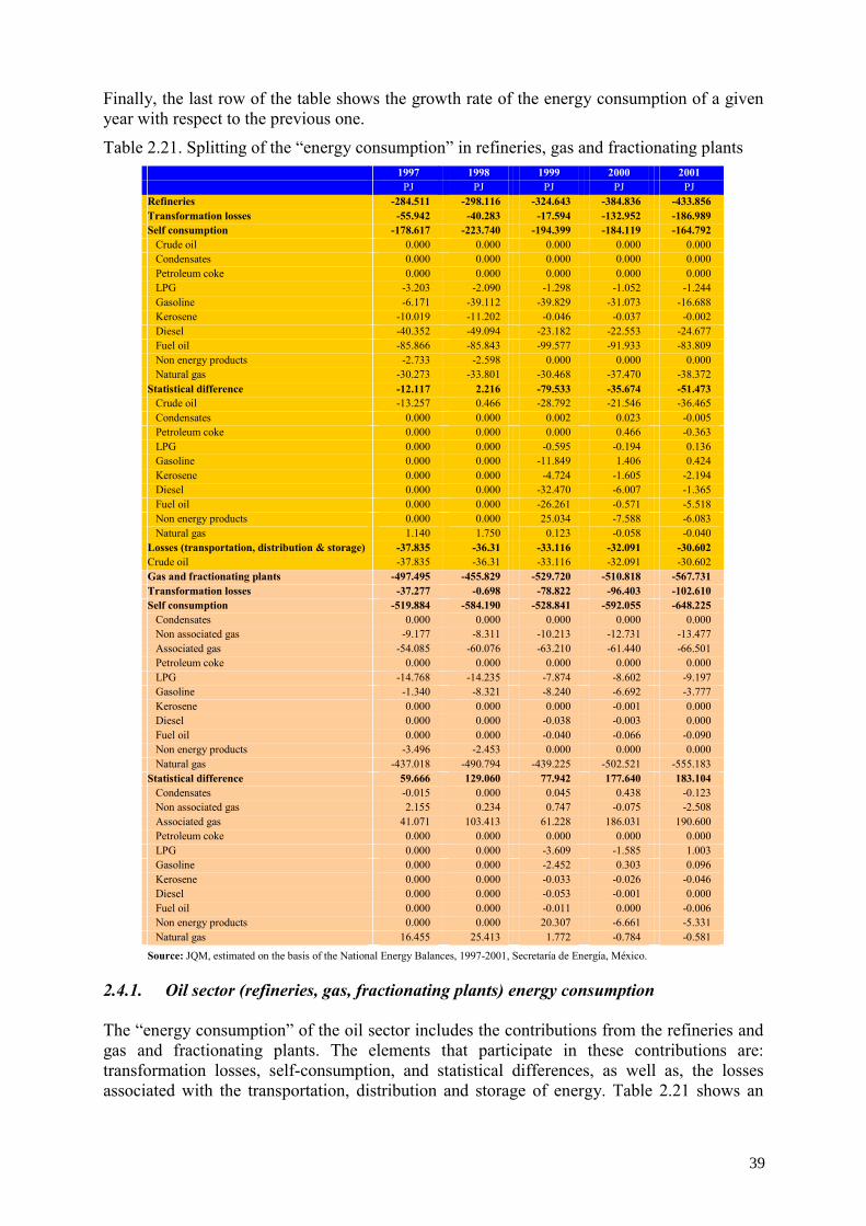
Finally, the last row of the table shows the growth rate of the energy consumption of a given year with respect to the previous one.

Table 2.21. Splitting of the “energy consumption” in refineries, gas and fractionating plants 1997 1998 1999 2000 2001 PJ PJ PJ PJ PJ Refineries -284.511 -298.116 -324.643 -384.836 -433.856 Transformation losses -55.942 -40.283 -17.594 -132.952 -186.989 Self consumption -178.617 -223.740 -194.399 -184.119 -164.792

Crude oil 0.000 0.000 0.000 0.000 0.000 Condensates 0.000 0.000 0.000 0.000 0.000 Petroleum coke 0.000 0.000 0.000 0.000 0.000 LPG -3.203 -2.090 -1.298 -1.052 -1.244 Gasoline -6.171 -39.112 -39.829 -31.073 -16.688 Kerosene -10.019 -11.202 -0.046 -0.037 -0.002 Diesel -40.352 -49.094 -23.182 -22.553 -24.677 Fuel oil -85.866 -85.843 -99.577 -91.933 -83.809 Non energy products -2.733 -2.598 0.000 0.000 0.000 Natural gas -30.273 -33.801 -30.468 -37.470 -38.372

Statistical difference -12.117 2.216 -79.533 -35.674 -51.473 Crude oil -13.257 0.466 -28.792 -21.546 -36.465 Condensates 0.000 0.000 0.002 0.023 -0.005 Petroleum coke 0.000 0.000 0.000 0.466 -0.363 LPG 0.000 0.000 -0.595 -0.194 0.136 Gasoline 0.000 0.000 -11.849 1.406 0.424 Kerosene 0.000 0.000 -4.724 -1.605 -2.194 Diesel 0.000 0.000 -32.470 -6.007 -1.365 Fuel oil 0.000 0.000 -26.261 -0.571 -5.518 Non energy products 0.000 0.000 25.034 -7.588 -6.083 Natural gas 1.140 1.750 0.123 -0.058 -0.040

Losses (transportation, distribution & storage) -37.835 -36.31 -33.116 -32.091 -30.602 Crude oil -37.835 -36.31 -33.116 -32.091 -30.602 Gas and fractionating plants -497.495 -455.829 -529.720 -510.818 -567.731 Transformation losses -37.277 -0.698 -78.822 -96.403 -102.610 Self consumption -519.884 -584.190 -528.841 -592.055 -648.225

Condensates 0.000 0.000 0.000 0.000 0.000 Non associated gas -9.177 -8.311 -10.213 -12.731 -13.477 Associated gas -54.085 -60.076 -63.210 -61.440 -66.501 Petroleum coke 0.000 0.000 0.000 0.000 0.000 LPG -14.768 -14.235 -7.874 -8.602 -9.197 Gasoline -1.340 -8.321 -8.240 -6.692 -3.777 Kerosene 0.000 0.000 0.000 -0.001 0.000 Diesel 0.000 0.000 -0.038 -0.003 0.000 Fuel oil 0.000 0.000 -0.040 -0.066 -0.090 Non energy products -3.496 -2.453 0.000 0.000 0.000 Natural gas -437.018 -490.794 -439.225 -502.521 -555.183

Statistical difference 59.666 129.060 77.942 177.640 183.104 Condensates -0.015 0.000 0.045 0.438 -0.123 Non associated gas 2.155 0.234 0.747 -0.075 -2.508 Associated gas 41.071 103.413 61.228 186.031 190.600 Petroleum coke 0.000 0.000 0.000 0.000 0.000 LPG 0.000 0.000 -3.609 -1.585 1.003 Gasoline 0.000 0.000 -2.452 0.303 0.096 Kerosene 0.000 0.000 -0.033 -0.026 -0.046 Diesel 0.000 0.000 -0.053 -0.001 0.000 Fuel oil 0.000 0.000 -0.011 0.000 -0.006 Non energy products 0.000 0.000 20.307 -6.661 -5.331 Natural gas 16.455 25.413 1.772 -0.784 -0.581

Source: JQM, estimated on the basis of the National Energy Balances, 1997-2001, Secretaría de Energía, México. 2.4.1. Oil sector (refineries, gas, fractionating plants) energy consumption The “energy consumption” of the oil sector includes the contributions from the refineries and gas and fractionating plants. The elements that participate in these contributions are: transformation losses, self-consumption, and statistical differences, as well as, the losses associated with the transportation, distribution and storage of energy. Table 2.21 shows an

39

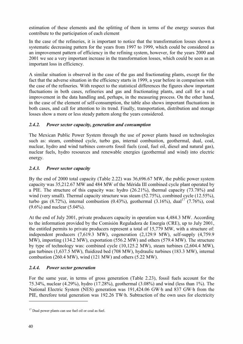
estimation of these elements and the splitting of them in terms of the energy sources that contribute to the participation of each element

In the case of the refineries, it is important to notice that the transformation losses shown a systematic decreasing pattern for the years from 1997 to 1999, which could be considered as an improvement pattern of efficiency in the refining system, however, for the years 2000 and 2001 we see a very important increase in the transformation losses, which could be seen as an important loss in efficiency.

A similar situation is observed in the case of the gas and fractionating plants, except for the fact that the adverse situation in the efficiency starts in 1999, a year before in comparison with the case of the refineries. With respect to the statistical differences the figures show important fluctuations in both cases, refineries and gas and fractionating plants, and call for a real improvement in the data handling and, perhaps, in the measuring process. On the other hand, in the case of the element of self-consumption, the table also shows important fluctuations in both cases, and call for attention to its trend. Finally, transportation, distribution and storage losses show a more or less steady pattern along the years considered.

2.4.2. Power sector capacity, generation and consumption

The Mexican Public Power System through the use of power plants based on technologies such as: steam, combined cycle, turbo gas, internal combustion, geothermal, dual, coal, nuclear, hydro and wind turbines converts fossil fuels (coal, fuel oil, diesel and natural gas), nuclear fuels, hydro resources and renewable energies (geothermal and wind) into electric energy.

2.4.3. Power sector capacity

By the end of 2000 total capacity (Table 2.22) was 36,696.67 MW, the public power system capacity was 35,212.67 MW and 484 MW of the Mérida III combined cycle plant operated by a PIE. The structure of this capacity was: hydro (26.21%), thermal capacity (73.78%) and wind (very small). Thermal capacity structure was steam (52.75%), combined cycle (12.55%), turbo gas (8.72%), internal combustion (0.43%), geothermal (3.16%), dual17 (7.76%), coal (9.6%) and nuclear (5.04%).

At the end of July 2001, private producers capacity in operation was 4,484.3 MW. According to the information provided by the Comisión Reguladora de Energía (CRE), up to July 2001, the entitled permits to private producers represent a total of 15,779 MW, with a structure of: independent producers (7,619.3 MW), cogeneration (2,129.9 MW), self-supply (4,759.9 MW), importing (134.2 MW), exportation (556.2 MW) and others (579.4 MW). The structure by type of technology was: combined cycle (10,125.2 MW), steam turbines (2,604.4 MW), gas turbines (1,637.5 MW), fluidized bed (708 MW), hydraulic turbines (183.3 MW), internal combustion (260.4 MW), wind (121 MW) and others (5.22 MW).

2.4.4. Power sector generation

For the same year, in terms of gross generation (Table 2.23), fossil fuels account for the 75.34%, nuclear (4.29%), hydro (17.28%), geothermal (3.08%) and wind (less than 1%). The National Electric System (NES) generation was 191,424.06 GW·h and 837 GW·h from the PIE, therefore total generation was 192.26 TW·h. Subtraction of the own uses for electricity 17 Dual power plants can use fuel oil or coal as fuel.

40

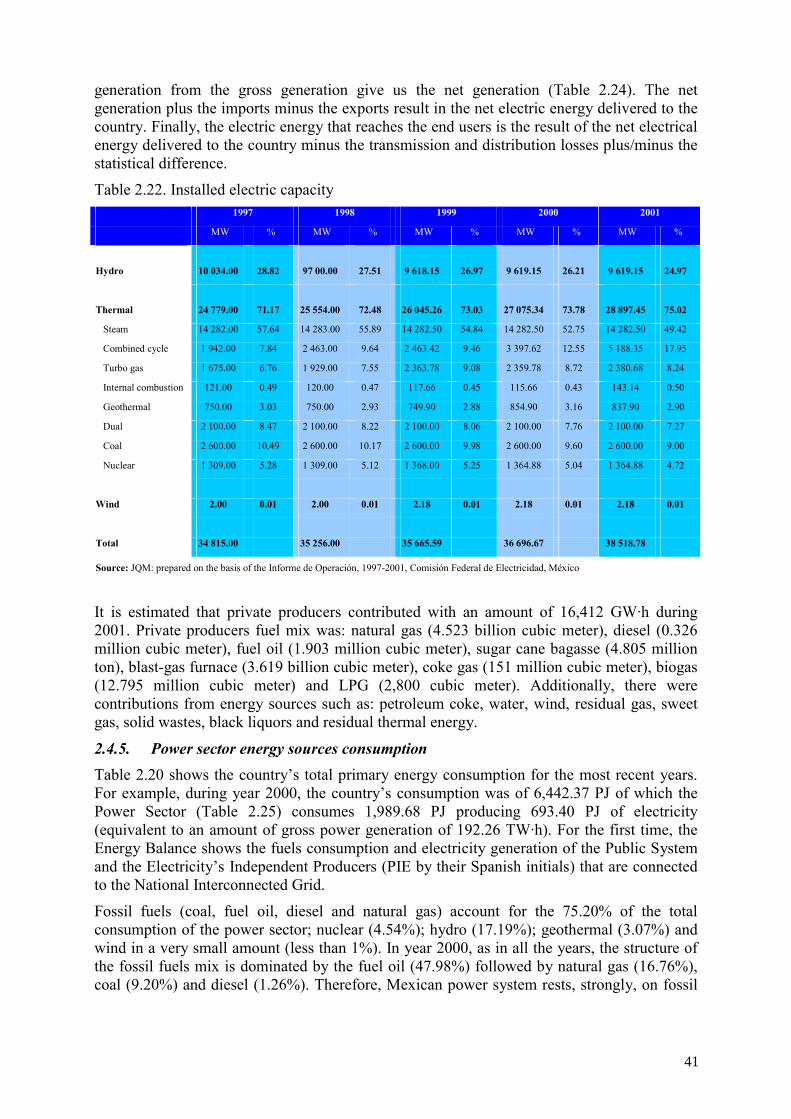
generation from the gross generation give us the net generation (Table 2.24). The net generation plus the imports minus the exports result in the net electric energy delivered to the country. Finally, the electric energy that reaches the end users is the result of the net electrical energy delivered to the country minus the transmission and distribution losses plus/minus the statistical difference.

Table 2.22. Installed electric capacity 1997 1998 1999 2000 2001

MW % MW % MW % MW % MW %

Hydro 10 034.00 28.82 97 00.00 27.51 9 618.15 26.97 9 619.15 26.21 9 619.15 24.97

Thermal 24 779.00 71.17 25 554.00 72.48 26 045.26 73.03 27 075.34 73.78 28 897.45 75.02

Steam 14 282.00 57.64 14 283.00 55.89 14 282.50 54.84 14 282.50 52.75 14 282.50 49.42

Combined cycle 1 942.00 7.84 2 463.00 9.64 2 463.42 9.46 3 397.62 12.55 5 188.35 17.95

Turbo gas 1 675.00 6.76 1 929.00 7.55 2 363.78 9.08 2 359.78 8.72 2 380.68 8.24

Internal combustion 121.00 0.49 120.00 0.47 117.66 0.45 115.66 0.43 143.14 0.50

Geothermal 750.00 3.03 750.00 2.93 749.90 2.88 854.90 3.16 837.90 2.90

Dual 2 100.00 8.47 2 100.00 8.22 2 100.00 8.06 2 100.00 7.76 2 100.00 7.27

Coal 2 600.00 10.49 2 600.00 10.17 2 600.00 9.98 2 600.00 9.60 2 600.00 9.00

Nuclear 1 309.00 5.28 1 309.00 5.12 1 368.00 5.25 1 364.88 5.04 1 364.88 4.72

Wind 2.00 0.01 2.00 0.01 2.18 0.01 2.18 0.01 2.18 0.01

Total 34 815.00 35 256.00 35 665.59 36 696.67 38 518.78

Source: JQM: prepared on the basis of the Informe de Operación, 1997-2001, Comisión Federal de Electricidad, México

It is estimated that private producers contributed with an amount of 16,412 GW·h during 2001. Private producers fuel mix was: natural gas (4.523 billion cubic meter), diesel (0.326 million cubic meter), fuel oil (1.903 million cubic meter), sugar cane bagasse (4.805 million ton), blast-gas furnace (3.619 billion cubic meter), coke gas (151 million cubic meter), biogas (12.795 million cubic meter) and LPG (2,800 cubic meter). Additionally, there were contributions from energy sources such as: petroleum coke, water, wind, residual gas, sweet gas, solid wastes, black liquors and residual thermal energy.

2.4.5. Power sector energy sources consumption Table 2.20 shows the country’s total primary energy consumption for the most recent years. For example, during year 2000, the country’s consumption was of 6,442.37 PJ of which the Power Sector (Table 2.25) consumes 1,989.68 PJ producing 693.40 PJ of electricity (equivalent to an amount of gross power generation of 192.26 TW·h). For the first time, the Energy Balance shows the fuels consumption and electricity generation of the Public System and the Electricity’s Independent Producers (PIE by their Spanish initials) that are connected to the National Interconnected Grid.

Fossil fuels (coal, fuel oil, diesel and natural gas) account for the 75.20% of the total consumption of the power sector; nuclear (4.54%); hydro (17.19%); geothermal (3.07%) and wind in a very small amount (less than 1%). In year 2000, as in all the years, the structure of the fossil fuels mix is dominated by the fuel oil (47.98%) followed by natural gas (16.76%), coal (9.20%) and diesel (1.26%). Therefore, Mexican power system rests, strongly, on fossil

41

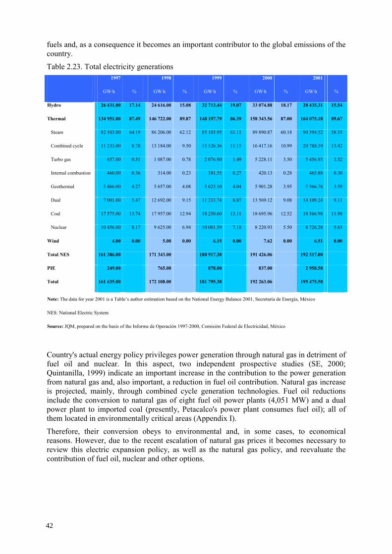
fuels and, as a consequence it becomes an important contributor to the global emissions of the country.

Table 2.23. Total electricity generations 1997 1998 1999 2000 2001

GW·h % GW·h % GW·h % GW·h % GW·h %

Hydro 26 431.00 17.14 24 616.00 15.08 32 713.44 19.07 33 074.88 18.17 28 435.31 15.54

Thermal 134 951.00 87.49 146 722.00 89.87 148 197.79 86.39 158 343.56 87.00 164 075.18 89.67

Steam 82 103.00 64.19 86 206.00 62.12 85 103.95 61.11 89 890.87 60.18 90 394.52 58.35

Combined cycle 11 233.00 8.78 13 184.00 9.50 15 526.36 11.15 16 417.16 10.99 20 788.59 13.42

Turbo gas 657.00 0.51 1 087.00 0.78 2 076.90 1.49 5 228.11 3.50 5 456.93 3.52


Geothermal 5 466.00 4.27 5 657.00 4.08 5 623.10 4.04 5 901.28 3.95 5 566.76 3.59

Dual 7 001.00 5.47 12 692.00 9.15 11 233.74 8.07 13 569.12 9.08 14 109.24 9.11

Coal 17 575.00 13.74 17 957.00 12.94 18 250.60 13.11 18 695.96 12.52 18 566.98 11.98

Nuclear 10 456.00 8.17 9 625.00 6.94 10 001.59 7.18 8 220.93 5.50 8 726.28 5.63

Wind 4.00 0.00 5.00 0.00 6.15 0.00 7.62 0.00 6.51 0.00

Total NES 161 386.00 171 343.00 180 917.38 191 426.06 192 517.00

PIE 249.00 765.00 878.00 837.00 2 958.58

Total 161 635.00 172 108.00 181 795.38 192 263.06 195 475.58

Note: The data for year 2001 is a Table’s author estimation based on the National Energy Balance 2001, Secretaría de Energía, México

NES: National Electric System

Source: JQM, prepared on the basis of the Informe de Operación 1997-2000, Comisión Federal de Electricidad, México

Country's actual energy policy privileges power generation through natural gas in detriment of fuel oil and nuclear. In this aspect, two independent prospective studies (SE, 2000; Quintanilla, 1999) indicate an important increase in the contribution to the power generation from natural gas and, also important, a reduction in fuel oil contribution. Natural gas increase is projected, mainly, through combined cycle generation technologies. Fuel oil reductions include the conversion to natural gas of eight fuel oil power plants (4,051 MW) and a dual power plant to imported coal (presently, Petacalco's power plant consumes fuel oil); all of them located in environmentally critical areas (Appendix I).

Therefore, their conversion obeys to environmental and, in some cases, to economical reasons. However, due to the recent escalation of natural gas prices it becomes necessary to review this electric expansion policy, as well as the natural gas policy, and reevaluate the contribution of fuel oil, nuclear and other options.

42

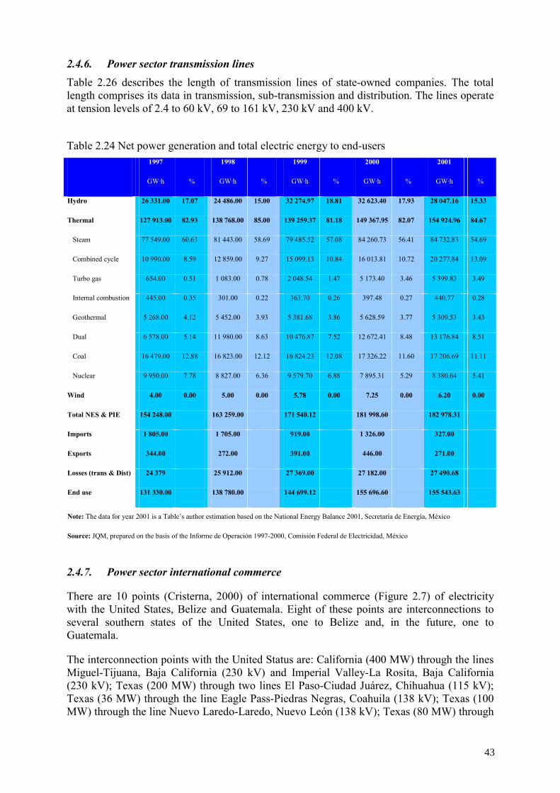
2.4.6. Power sector transmission lines Table 2.26 describes the length of transmission lines of state-owned companies. The total length comprises its data in transmission, sub-transmission and distribution. The lines operate at tension levels of 2.4 to 60 kV, 69 to 161 kV, 230 kV and 400 kV.

Table 2.24 Net power generation and total electric energy to end-users 1997 1998 1999 2000 2001

GW·h % GW·h % GW·h % GW·h % GW·h %

Hydro 26 331.00 17.07 24 486.00 15.00 32 274.97 18.81 32 623.40 17.93 28 047.16 15.33

Thermal 127 913.00 82.93 138 768.00 85.00 139 259.37 81.18 149 367.95 82.07 154 924.96 84.67

Steam 77 549.00 60.63 81 443.00 58.69 79 485.52 57.08 84 260.73 56.41 84 732.83 54.69

Combined cycle 10 990.00 8.59 12 859.00 9.27 15 099.13 10.84 16 013.81 10.72 20 277.84 13.09

Turbo gas 654.00 0.51 1 083.00 0.78 2 048.54 1.47 5 173.40 3.46 5 399.83 3.49


Geothermal 5 268.00 4.12 5 452.00 3.93 5 381.68 3.86 5 628.59 3.77 5 309.53 3.43

Dual 6 578.00 5.14 11 980.00 8.63 10 476.87 7.52 12 672.41 8.48 13 176.84 8.51

Coal 16 479.00 12.88 16 823.00 12.12 16 824.23 12.08 17 326.22 11.60 17 206.69 11.11

Nuclear 9 950.00 7.78 8 827.00 6.36 9 579.70 6.88 7 895.31 5.29 8 380.64 5.41

Wind 4.00 0.00 5.00 0.00 5.78 0.00 7.25 0.00 6.20 0.00

Total NES & PIE 154 248.00 163 259.00 171 540.12 181 998.60 182 978.31

Imports 1 805.00 1 705.00 919.00 1 326.00 327.00

Exports 344.00 272.00 391.00 446.00 271.00

Losses (trans & Dist) 24 379 25 912.00 27 369.00 27 182.00 27 490.68

End use 131 330.00 138 780.00 144 699.12 155 696.60 155 543.63

Note: The data for year 2001 is a Table’s author estimation based on the National Energy Balance 2001, Secretaría de Energía, México

Source: JQM, prepared on the basis of the Informe de Operación 1997-2000, Comisión Federal de Electricidad, México

2.4.7. Power sector international commerce

There are 10 points (Cristerna, 2000) of international commerce (Figure 2.7) of electricity with the United States, Belize and Guatemala. Eight of these points are interconnections to several southern states of the United States, one to Belize and, in the future, one to Guatemala.

The interconnection points with the United Status are: California (400 MW) through the lines Miguel-Tijuana, Baja California (230 kV) and Imperial Valley-La Rosita, Baja California (230 kV); Texas (200 MW) through two lines El Paso-Ciudad Juárez, Chihuahua (115 kV); Texas (36 MW) through the line Eagle Pass-Piedras Negras, Coahuila (138 kV); Texas (100 MW) through the line Nuevo Laredo-Laredo, Nuevo León (138 kV); Texas (80 MW) through

43

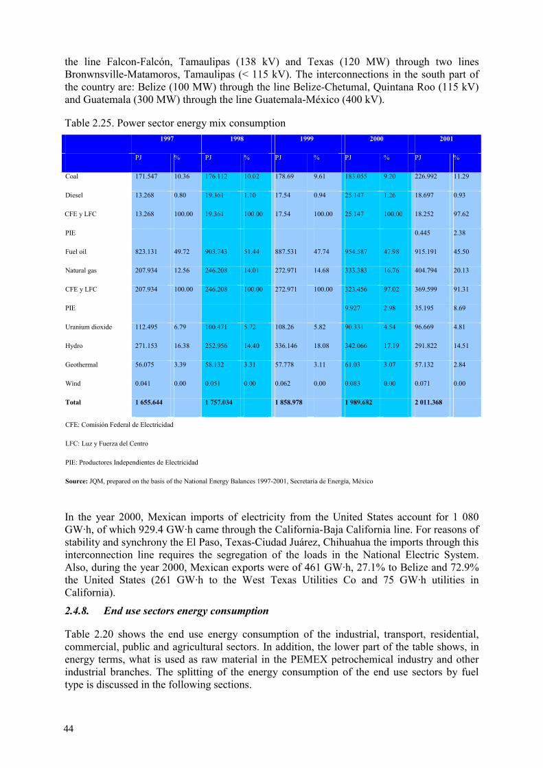
the line Falcon-Falcón, Tamaulipas (138 kV) and Texas (120 MW) through two lines Bronwnsville-Matamoros, Tamaulipas (< 115 kV). The interconnections in the south part of the country are: Belize (100 MW) through the line Belize-Chetumal, Quintana Roo (115 kV) and Guatemala (300 MW) through the line Guatemala-México (400 kV).

Table 2.25. Power sector energy mix consumption 1997 1998 1999 2000 2001


Coal 171.547 10.36 176.112 10.02 178.69 9.61 183.055 9.20 226.992 11.29

Diesel 13.268 0.80 19.361 1.10 17.54 0.94 25.147 1.26 18.697 0.93

CFE y LFC 13.268 100.00 19.361 100.00 17.54 100.00 25.147 100.00 18.252 97.62

PIE 0.445 2.38

Fuel oil 823.131 49.72 903.743 51.44 887.531 47.74 954.587 47.98 915.191 45.50

Natural gas 207.934 12.56 246.208 14.01 272.971 14.68 333.383 16.76 404.794 20.13

CFE y LFC 207.934 100.00 246.208 100.00 272.971 100.00 323.456 97.02 369.599 91.31

PIE 9.927 2.98 35.195 8.69

Uranium dioxide 112.495 6.79 100.471 5.72 108.26 5.82 90.331 4.54 96.669 4.81

Hydro 271.153 16.38 252.956 14.40 336.146 18.08 342.066 17.19 291.822 14.51

Geothermal 56.075 3.39 58.132 3.31 57.778 3.11 61.03 3.07 57.132 2.84

Wind 0.041 0.00 0.051 0.00 0.062 0.00 0.083 0.00 0.071 0.00

Total 1 655.644 1 757.034 1 858.978 1 989.682 2 011.368

CFE: Comisión Federal de Electricidad

LFC: Luz y Fuerza del Centro

PIE: Productores Independientes de Electricidad

Source: JQM, prepared on the basis of the National Energy Balances 1997-2001, Secretaría de Energía, México

In the year 2000, Mexican imports of electricity from the United States account for 1 080 GW·h, of which 929.4 GW·h came through the California-Baja California line. For reasons of stability and synchrony the El Paso, Texas-Ciudad Juárez, Chihuahua the imports through this interconnection line requires the segregation of the loads in the National Electric System. Also, during the year 2000, Mexican exports were of 461 GW·h, 27.1% to Belize and 72.9% the United States (261 GW·h to the West Texas Utilities Co and 75 GW·h utilities in California).

2.4.8. End use sectors energy consumption

Table 2.20 shows the end use energy consumption of the industrial, transport, residential, commercial, public and agricultural sectors. In addition, the lower part of the table shows, in energy terms, what is used as raw material in the PEMEX petrochemical industry and other industrial branches. The splitting of the energy consumption of the end use sectors by fuel type is discussed in the following sections.

44

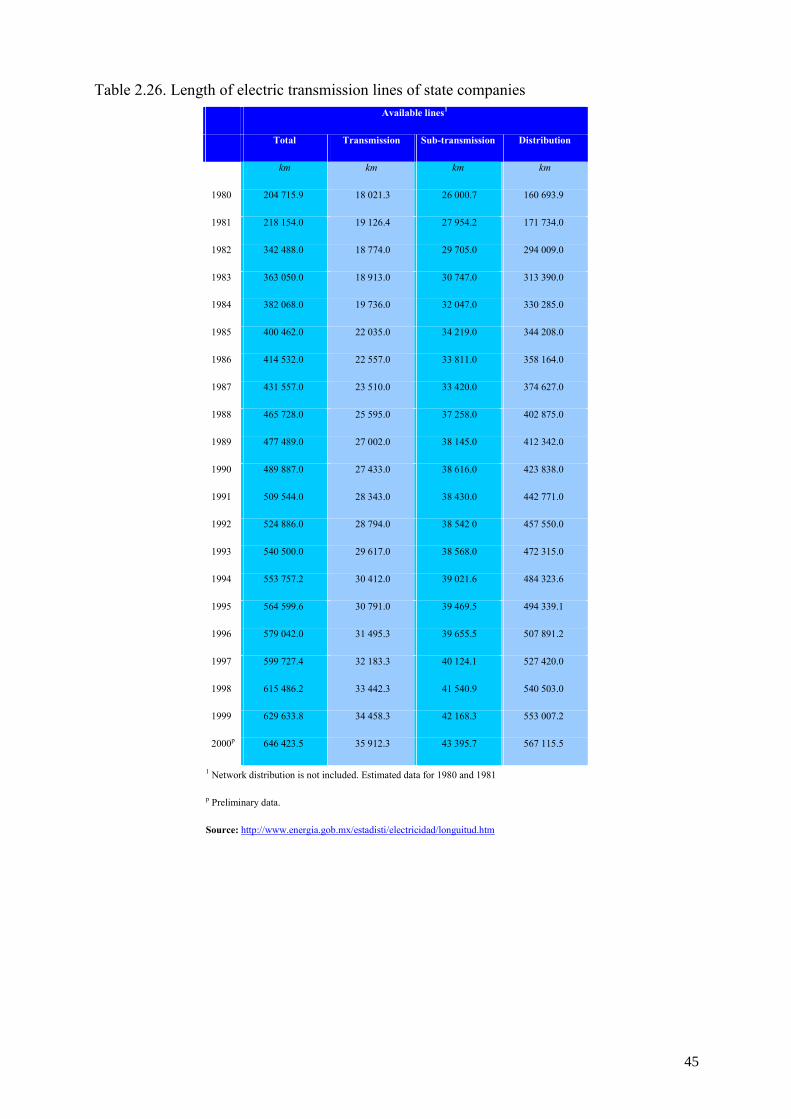
Table 2.26. Length of electric transmission lines of state companies Available lines1

Total Transmission Sub-transmission Distribution

km km km km

1980 204 715.9 18 021.3 26 000.7 160 693.9

1981 218 154.0 19 126.4 27 954.2 171 734.0

1982 342 488.0 18 774.0 29 705.0 294 009.0

1983 363 050.0 18 913.0 30 747.0 313 390.0

1984 382 068.0 19 736.0 32 047.0 330 285.0

1985 400 462.0 22 035.0 34 219.0 344 208.0

1986 414 532.0 22 557.0 33 811.0 358 164.0

1987 431 557.0 23 510.0 33 420.0 374 627.0

1988 465 728.0 25 595.0 37 258.0 402 875.0

1989 477 489.0 27 002.0 38 145.0 412 342.0

1990 489 887.0 27 433.0 38 616.0 423 838.0

1991 509 544.0 28 343.0 38 430.0 442 771.0

1992 524 886.0 28 794.0 38 542 0 457 550.0

1993 540 500.0 29 617.0 38 568.0 472 315.0

1994 553 757.2 30 412.0 39 021.6 484 323.6

1995 564 599.6 30 791.0 39 469.5 494 339.1

1996 579 042.0 31 495.3 39 655.5 507 891.2

1997 599 727.4 32 183.3 40 124.1 527 420.0

1998 615 486.2 33 442.3 41 540.9 540 503.0

1999 629 633.8 34 458.3 42 168.3 553 007.2

2000p 646 423.5 35 912.3 43 395.7 567 115.5

1 Network distribution is not included. Estimated data for 1980 and 1981

p Preliminary data.

Source: http://www.energia.gob.mx/estadisti/electricidad/longuitud.htm

45

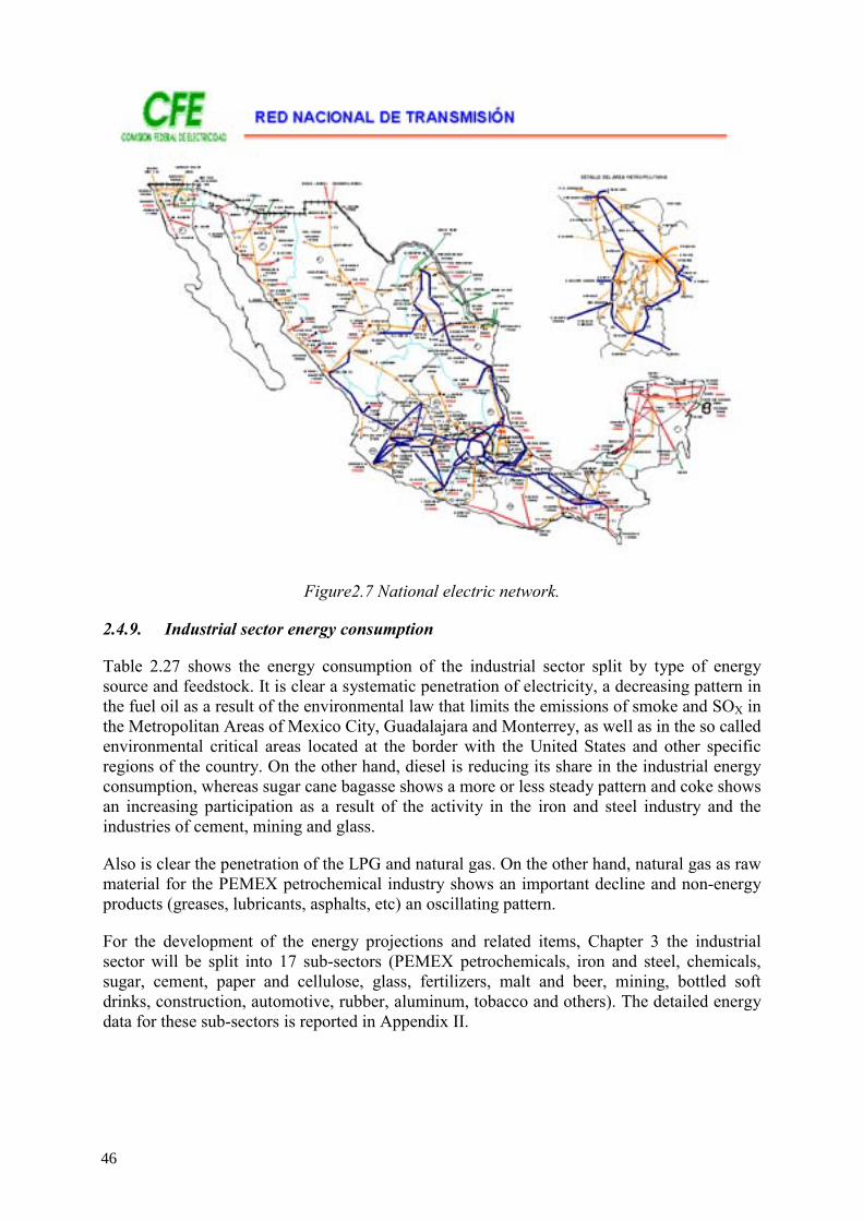
Figure2.7 National electric network.

2.4.9. Industrial sector energy consumption

Table 2.27 shows the energy consumption of the industrial sector split by type of energy source and feedstock. It is clear a systematic penetration of electricity, a decreasing pattern in the fuel oil as a result of the environmental law that limits the emissions of smoke and SOX in the Metropolitan Areas of Mexico City, Guadalajara and Monterrey, as well as in the so called environmental critical areas located at the border with the United States and other specific regions of the country. On the other hand, diesel is reducing its share in the industrial energy consumption, whereas sugar cane bagasse shows a more or less steady pattern and coke shows an increasing participation as a result of the activity in the iron and steel industry and the industries of cement, mining and glass.

Also is clear the penetration of the LPG and natural gas. On the other hand, natural gas as raw material for the PEMEX petrochemical industry shows an important decline and non-energy products (greases, lubricants, asphalts, etc) an oscillating pattern.

For the development of the energy projections and related items, Chapter 3 the industrial sector will be split into 17 sub-sectors (PEMEX petrochemicals, iron and steel, chemicals, sugar, cement, paper and cellulose, glass, fertilizers, malt and beer, mining, bottled soft drinks, construction, automotive, rubber, aluminum, tobacco and others). The detailed energy data for these sub-sectors is reported in Appendix II.

46

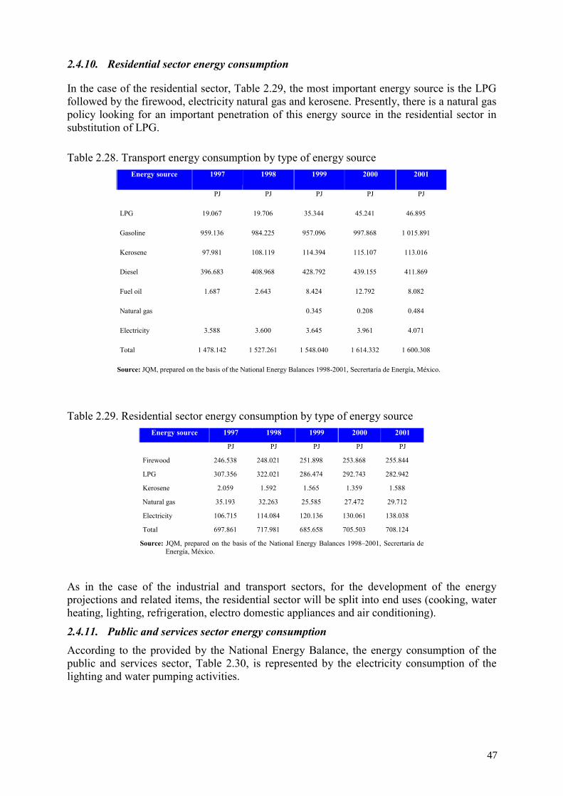
2.4.10. Residential sector energy consumption

In the case of the residential sector, Table 2.29, the most important energy source is the LPG followed by the firewood, electricity natural gas and kerosene. Presently, there is a natural gas policy looking for an important penetration of this energy source in the residential sector in substitution of LPG.

Table 2.28. Transport energy consumption by type of energy source Energy source 1997 1998 1999 2000 2001

PJ PJ PJ PJ PJ

LPG 19.067 19.706 35.344 45.241 46.895

Gasoline 959.136 984.225 957.096 997.868 1 015.891

Kerosene 97.981 108.119 114.394 115.107 113.016

Diesel 396.683 408.968 428.792 439.155 411.869

Fuel oil 1.687 2.643 8.424 12.792 8.082

Natural gas 0.345 0.208 0.484

Electricity 3.588 3.600 3.645 3.961 4.071

Total 1 478.142 1 527.261 1 548.040 1 614.332 1 600.308

Source: JQM, prepared on the basis of the National Energy Balances 1998-2001, Secrertaría de Energía, México.

Table 2.29. Residential sector energy consumption by type of energy source Energy source 1997 1998 1999 2000 2001

PJ PJ PJ PJ PJ

Firewood 246.538 248.021 251.898 253.868 255.844

LPG 307.356 322.021 286.474 292.743 282.942

Kerosene 2.059 1.592 1.565 1.359 1.588

Natural gas 35.193 32.263 25.585 27.472 29.712

Electricity 106.715 114.084 120.136 130.061 138.038

Total 697.861 717.981 685.658 705.503 708.124

Source: JQM, prepared on the basis of the National Energy Balances 1998–2001, Secrertaría de Energía, México.

As in the case of the industrial and transport sectors, for the development of the energy projections and related items, the residential sector will be split into end uses (cooking, water heating, lighting, refrigeration, electro domestic appliances and air conditioning).

2.4.11. Public and services sector energy consumption According to the provided by the National Energy Balance, the energy consumption of the public and services sector, Table 2.30, is represented by the electricity consumption of the lighting and water pumping activities.

47

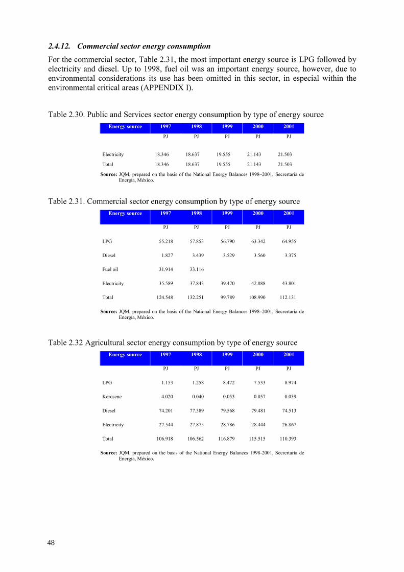
2.4.12. Commercial sector energy consumption For the commercial sector, Table 2.31, the most important energy source is LPG followed by electricity and diesel. Up to 1998, fuel oil was an important energy source, however, due to environmental considerations its use has been omitted in this sector, in especial within the environmental critical areas (APPENDIX I).

Table 2.30. Public and Services sector energy consumption by type of energy source Energy source 1997 1998 1999 2000 2001

PJ PJ PJ PJ PJ

Electricity 18.346 18.637 19.555 21.143 21.503

Total 18.346 18.637 19.555 21.143 21.503


Table 2.31. Commercial sector energy consumption by type of energy source

Energy source 1997 1998 1999 2000 2001

PJ PJ PJ PJ PJ

LPG 55.218 57.853 56.790 63.342 64.955

Diesel 1.827 3.439 3.529 3.560 3.375

Fuel oil 31.914 33.116

Electricity 35.589 37.843 39.470 42.088 43.801

Total 124.548 132.251 99.789 108.990 112.131


Table 2.32 Agricultural sector energy consumption by type of energy source

Energy source 1997 1998 1999 2000 2001

PJ PJ PJ PJ PJ

LPG 1.153 1.258 8.472 7.533 8.974

Kerosene 4.020 0.040 0.053 0.057 0.039

Diesel 74.201 77.389 79.568 79.481 74.513

Electricity 27.544 27.875 28.786 28.444 26.867

Total 106.918 106.562 116.879 115.515 110.393

Source: JQM, prepared on the basis of the National Energy Balances 1998-2001, Secrertaría de Energía, México.

48

2.4.13. Agricultural sector energy consumption In the case of the agricultural sector, Table 2.32, the most important energy source is the diesel, which shows a more or less steady pattern, followed by electricity also with a steady pattern, an increasing pattern of LPG and a decreasing one in the case of kerosene.

Finally, in the Appendix C the reader will find a presentation of the current organization and policies in the energy sector, as well as, energy planning procedures in the oil and electric sectors. Appendix I contains a presentation of the environmental legislation and policies related to the use of energy in the sectors.

49

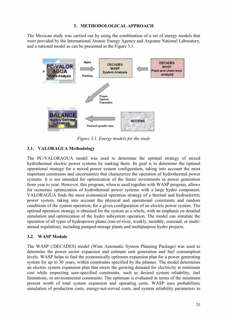
3. METHODOLOGICAL APPROACH

The Mexican study was carried out by using the combination of a set of energy models that were provided by the International Atomic Energy Agency and Argonne National Laboratory, and a national model as can be presented in the Figure 3.1.

Figure 3.1. Energy models for the study

3.1. VALORAGUA Methodology

The PC-VALORAGUA model was used to determine the optimal strategy of mixed hydrothermal electric power systems by ranking them. Its goal is to determine the optimal operational strategy for a mixed power system configuration, taking into account the most important constraints and uncertainties that characterize the operation of hydrothermal power systems. It is not intended for optimization of the future investments in power generation from year to year. However, this program, when is used together with WASP program, allows for economic optimization of hydrothermal power systems with a large hydro component. VALORAGUA finds the most economical operation strategy of a thermal and hydroelectric power system, taking into account the physical and operational constraints and random conditions of the system operation, for a given configuration of an electric power system. The optimal operation strategy is obtained for the system as a whole, with an emphasis on detailed simulation and optimization of the hydro subsystem operation. The model can simulate the operation of all types of hydropower plants (run-of-river, weekly, monthly, seasonal, or multi-annual regulation), including pumped-storage plants and multipurpose hydro projects.

3.2. WASP Module

The WASP (/DECADES) model (Wien Automatic System Planning Package) was used to determine the power sector expansion and estimate unit generation and fuel consumption levels. WASP helps to find the economically optimum expansion plan for a power generating system for up to 30 years, within constraints specified by the planner. The model determines an electric system expansion plan that meets the growing demand for electricity at minimum cost while respecting user-specified constraints, such as desired system reliability, fuel limitations, or environmental constraints. The optimum is evaluated in terms of the minimum present worth of total system expansion and operating costs. WASP uses probabilistic simulation of production costs, energy-not-served costs, and system reliability parameters to

51

compare total costs of alternative expansion policies. Each possible sequence of power units added to the system (expansion plan or policy) that meets the constraints specified by the user is evaluated by a cost function (the objective function). The optimal expansion path is then determined using a dynamic programming algorithm. For the analysis of mixed hydrothermal power systems, WASP is frequently used in combination with the PC-VALORAGUA model. The expansion analysis conducted with the WASP/VALORAGUA methodology provides an enhanced representation of hydro power plants and their operation in the electric power system.

3.3. DECADES methodology

DECADES model was used for the first phase of the project, entitled: “Comparative Assessment of Energy Sources for Electricity Supply until 2025” (see Chapter 6 for the discussion and results) and its results of the power system expansion analysis were transferred to ENPEP model.

DECADES stands for an integrated software package of databases and methodologies for comparative assessment of different energy sources for electricity generation. It was developed to provide senior analysts and energy planners with an easy to use tool for carrying out decision support studies for the power sector. This tool consist of: 1) databases providing a set of technical, economic and environmental data for energy chains that use fossil fuels, nuclear power and renewable energy sources for electricity generation; 2) a data management system; 3) an analytical software designed to access the information stored in the databases for analysis of costs and environmental burdens at the power plant, full energy chain and electric levels and 4) a decision analysis tool.

The DECADES tools support three levels of analysis:

• Plant level analysis is used for preliminary screening of different electricity generation options. Emission factors for main air pollutants are estimated base on fuel characteristics and power plant performances. A modular representation of pollution abatement technologies allow for user specification of appropriate abatement technology effects on capital costs, fixed and variable operating and maintenance costs, plant capacity, plant efficiency, reagent consumption and waste generation. Simple cases can be defined to compare power plants in terms of annual electricity costs, air emissions (direct and associated to materials used in construction and commissioning of power plants); solid waste generated and land use.

• Chain level analysis provides general data and analysis sufficient to present a broad view of the major trade-off between technical, economic, health and environmental aspects of energy chains. It supports the comparative assessment of full energy chains for electricity generation, from resource extraction to waste disposal. A flexible interface facilitates rapid construction of energy chain representation. Chain level results include: mass flow of fuels and waste, levelized cost of electricity generation and quantities of environmental burdens such as air pollution and total greenhouse gas emissions (CO2 equivalent), water effluents, solid waste generation and land use. Environmental burdens from auxiliary materials such as electricity, fuels, and material of construction and dismantling are also calculated. Direct comparisons of different energy chains are possible using a side-by-side display, combined with simple access to emissions, residuals and economic data. Scenarios,

52

in which a given mixture of energy chains meets a fixed demand, can be established and evaluated in terms of annual air emissions, solid waste and land use.

• System-level analysis allows users to quickly screen electric generation system expansion strategies and to conduct comprehensive studies to develop mixes of energy chains, which meet electricity demand for a country or region. The system level planning tool contains three electric system analysis options, ranging from preliminary analysis tools based on screening curves to sophisticated least cost optimization with dynamic programming. It has core features derived from the IAEA’s WASP model with an enhanced graphical interface, improved computation of environmental residuals (e.g. air pollutant emissions, land use and waste generation) and extensive reporting capabilities. The environmental residuals are estimated taking into account the full energy chains composing the system. The cost effectiveness of different air pollutant abatement strategies is also estimated.

3.4. MODEMA methodology

MODEMA model [Quintanilla, 1999] was used to develop the energy demand projections. MODEMA is an energy demand model whose projections consider the detailed behavior of the main energy consuming sectors and sub-sectors, as well as their projected consumptions and diversification possibilities. The model was developed by the Dirección General de Servicios de Cómputo Académico (DGSCA) and Programa Universitario de Energía (PUE), both institutions of the Universidad Nacional Autónoma de México (UNAM).

MODEMA is as a top-down simulation model for the primary and final energy demand. As a simulation model, the size and the sectoral structure of the energy demand are determined by the evolution of:

• The determining variables that, as a set, define the behavior of the socioeconomic activity, and

• Their causal relation with the energy demand.

The model breaks up the economy into sectors and sub-sectors, as shown in Figure 3.2, and analyses their participation in the national economy. In this way, the future total energy demand will depend of the economy and energy expectations of each sector and upon their relative weight. As a consequence, it allows for an individual analysis of the main sectors and thus gives a more representative energy demand projection than a general energy-gross domestic product (GDP) relationship.

Additionally, it has the option of introducing policy instruments, such as those seeking energy conservation and thus, of analyzing the effects of proposed policies on energy demand. Therefore the model provides the total energy demand projections and also includes the demand by type of energy source for the sectors and sub-sectors.

Table 3.1 shows the sectors, sub-sectors, energy sources, feed stocks and emissions that are included in the model. The energy sector incorporates its own consumption plus transport losses, distribution and storage. The industrial sector includes 17 industrial sub-sectors and includes the sources for energy consumption as well as those that are used as raw materials. The usually aggregated residential, commercial and public sector is split into its three components and the public sector includes the area of services. The transport sector is split

53

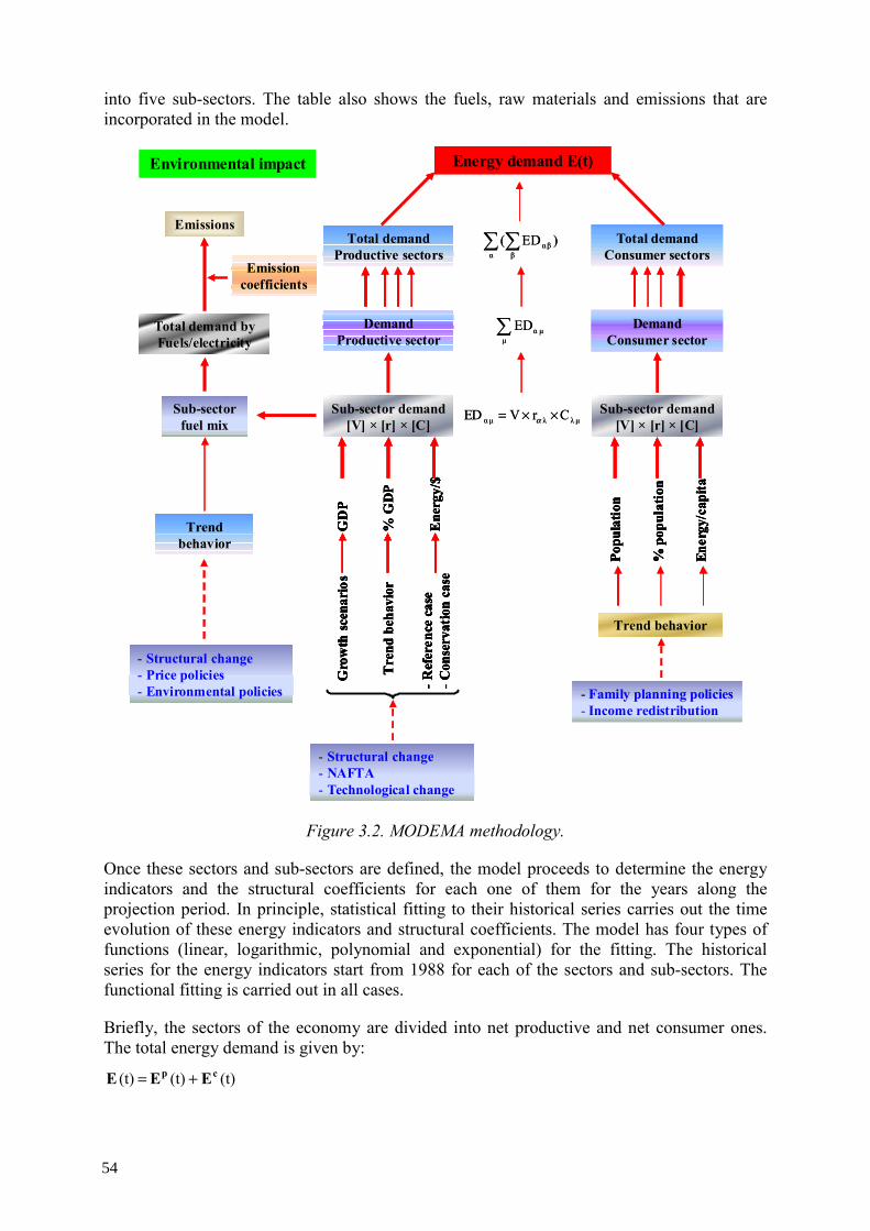
into five sub-sectors. The table also shows the fuels, raw materials and emissions that are incorporated in the model.

- Family planning policies- Income redistribution

Environmental impact Energy demand E(t)

Total demandProductive sectors

Total demandConsumer sectors

DemandProductive sector

DemandConsumer sector

Sub-sector demand[V] × [r] × [C]


∑ ∑α β

βα )ED(

∑µ

µαEDG

DP

% G

DP

Ene

rgy/

$

Popu

latio

n

% p

opul

atio

n

Ener

gy/c

apita

Gro

wth

sce

nari

os

Tre

nd b

ehav

ior

-Ref

eren

ce c

ase

-Con

serv

atio

n ca

se

Trend behavior

- Structural change- NAFTA- Technological change

Emissioncoefficients

Emissions

Total demand byFuels/electricity

Sub-sectorfuel mix

Trend behavior

- Structural change- Price policies- Environmental policies

µλλµα CrVED ××= α

- Family planning policies- Income redistribution

Environmental impact Energy demand E(t)

Total demandProductive sectors

Total demandConsumer sectors

DemandProductive sector

DemandConsumer sector



∑ ∑α β

βα )ED(

∑µ

µαEDG

DP

% G

DP

Ene

rgy/

$

GD

PG

DP

% G

DP

% G

DP

Ene

rgy/

$E

nerg

y/$

Popu

latio

n

% p

opul

atio

n

Ener

gy/c

apita

Popu

latio

nPo

pula

tion

% p

opul

atio

n%

pop

ulat

ion

Ener

gy/c

apita

Ener

gy/c

apita

Gro

wth

sce

nari

os

Tre

nd b

ehav

ior

-Ref

eren

ce c

ase

-Con

serv

atio

n ca

se

Gro

wth

sce

nari

osG

row

th s

cena

rios

Tre

nd b

ehav

ior

Tre

nd b

ehav

ior

-Ref

eren

ce c

ase

-Con

serv

atio

n ca

se-R

efer

ence

cas

e-C

onse

rvat

ion

case

Trend behavior

- Structural change- NAFTA- Technological change

Emissioncoefficients

Emissions

Total demand byFuels/electricity

Sub-sectorfuel mix

Trend behavior

- Structural change- Price policies- Environmental policies

µλλµα CrVED ××= α

Figure 3.2. MODEMA methodology.

Once these sectors and sub-sectors are defined, the model proceeds to determine the energy indicators and the structural coefficients for each one of them for the years along the projection period. In principle, statistical fitting to their historical series carries out the time evolution of these energy indicators and structural coefficients. The model has four types of functions (linear, logarithmic, polynomial and exponential) for the fitting. The historical series for the energy indicators start from 1988 for each of the sectors and sub-sectors. The functional fitting is carried out in all cases.

Briefly, the sectors of the economy are divided into net productive and net consumer ones. The total energy demand is given by:

(t)(t)(t) cp EEE +=

54

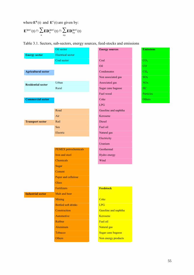
where (t)pE and (t)cE are given by:

∑ ∑α µα

)(µα

)(α

)( (t)(t)(t) cp,cp,cp, EDEDE ==

Table 3.1. Sectors, sub-sectors, energy sources, feed-stocks and emissions Oil sector Energy sources Emissions

Energy sector Electrical sector

Coal sector Coal CO2

Oil CO

Agricultural sector Condensates CH4

Non associated gas SOx

Urban Associated gas NOx Residential sector

Rural Sugar cane bagasse HC

Fuel wood Particles

Commercial sector Coke Others

LPG

Road Gasoline and naphtha

Air Kerosene

Transport sector Rail Diesel

Sea Fuel oil

Electric Natural gas

Electricity

Uranium

PEMEX petrochemicals Geothermal

Iron and steel Hydro energy

Chemicals Wind

Sugar

Cement

Paper and cellulose

Glass

Fertilizers Feedstock

Industrial sector Malt and beer

Mining Coke

Bottled soft drinks LPG

Construction Gasoline and naphtha

Automotive Kerosene

Rubber Fuel oil

Aluminum Natural gas

Tobacco Sugar cane bagasse

Others Non energy products

55

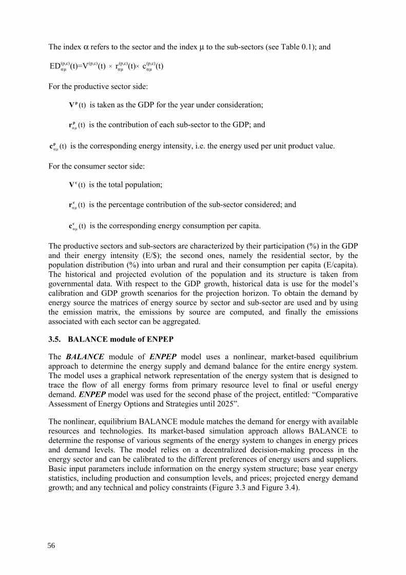
The index α refers to the sector and the index µ to the sub-sectors (see Table 0.1); and

(t)c(t)r(t)(t)=VED (p,c)µα

(p,c)µα

(p,c)(p,c)µα ××

For the productive sector side:

(t)pV is taken as the GDP for the year under consideration;

(t)µαpr is the contribution of each sub-sector to the GDP; and

(t)µαpc is the corresponding energy intensity, i.e. the energy used per unit product value.

For the consumer sector side:

(t)cV is the total population;

(t)µαcr is the percentage contribution of the sub-sector considered; and

(t)µαcc is the corresponding energy consumption per capita.

The productive sectors and sub-sectors are characterized by their participation (%) in the GDP and their energy intensity (E/$); the second ones, namely the residential sector, by the population distribution (%) into urban and rural and their consumption per capita (E/capita). The historical and projected evolution of the population and its structure is taken from governmental data. With respect to the GDP growth, historical data is use for the model’s calibration and GDP growth scenarios for the projection horizon. To obtain the demand by energy source the matrices of energy source by sector and sub-sector are used and by using the emission matrix, the emissions by source are computed, and finally the emissions associated with each sector can be aggregated.

3.5. BALANCE module of ENPEP

The BALANCE module of ENPEP model uses a nonlinear, market-based equilibrium approach to determine the energy supply and demand balance for the entire energy system. The model uses a graphical network representation of the energy system that is designed to trace the flow of all energy forms from primary resource level to final or useful energy demand. ENPEP model was used for the second phase of the project, entitled: “Comparative Assessment of Energy Options and Strategies until 2025”.

The nonlinear, equilibrium BALANCE module matches the demand for energy with available resources and technologies. Its market-based simulation approach allows BALANCE to determine the response of various segments of the energy system to changes in energy prices and demand levels. The model relies on a decentralized decision-making process in the energy sector and can be calibrated to the different preferences of energy users and suppliers. Basic input parameters include information on the energy system structure; base year energy statistics, including production and consumption levels, and prices; projected energy demand growth; and any technical and policy constraints (Figure 3.3 and Figure 3.4).

56

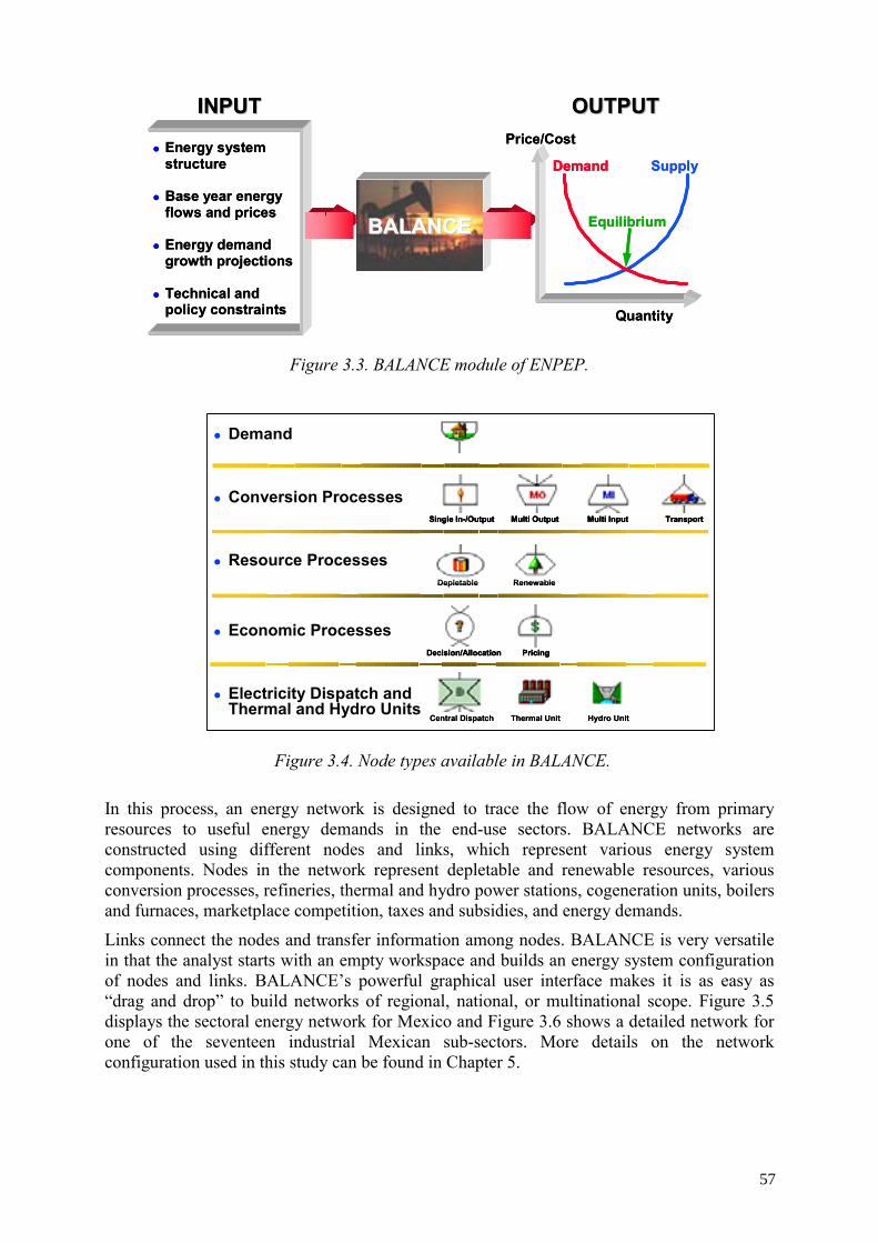
SupplySupplyDemand

Equilibrium

DemandDemand

Equilibrium

INPUTINPUT

Energy systemstructure

Base year energyflows and prices

Energy demandgrowth projections

Technical andpolicy constraints

INPUTINPUT

Energy systemstructure

Base year energyflows and prices

Energy demandgrowth projections

Technical andpolicy constraints

BALANCEBALANCE

OUTPUTOUTPUT

Quantity

Price/Cost

OUTPUTOUTPUT

Quantity

Price/Cost

Figure 3.3. BALANCE module of ENPEP.

Demand

Conversion Processes

Resource Processes

Economic Processes

Electricity Dispatch andThermal and Hydro Units

Single In-/Output Multi Output Multi Input TransportSingle In-/Output Multi Output Multi Input TransportSingle In-/Output Multi Output Multi Input Transport

Depletable RenewableDepletable Renewable

Decision/Allocation PricingDecision/Allocation PricingDecision/Allocation Pricing

Central Dispatch Thermal Unit Hydro UnitCentral Dispatch Thermal Unit Hydro Unit Figure 3.4. Node types available in BALANCE.

In this process, an energy network is designed to trace the flow of energy from primary resources to useful energy demands in the end-use sectors. BALANCE networks are constructed using different nodes and links, which represent various energy system components. Nodes in the network represent depletable and renewable resources, various conversion processes, refineries, thermal and hydro power stations, cogeneration units, boilers and furnaces, marketplace competition, taxes and subsidies, and energy demands.

Links connect the nodes and transfer information among nodes. BALANCE is very versatile in that the analyst starts with an empty workspace and builds an energy system configuration of nodes and links. BALANCE’s powerful graphical user interface makes it is as easy as “drag and drop” to build networks of regional, national, or multinational scope. Figure 3.5 displays the sectoral energy network for Mexico and Figure 3.6 shows a detailed network for one of the seventeen industrial Mexican sub-sectors. More details on the network configuration used in this study can be found in Chapter 5.

57

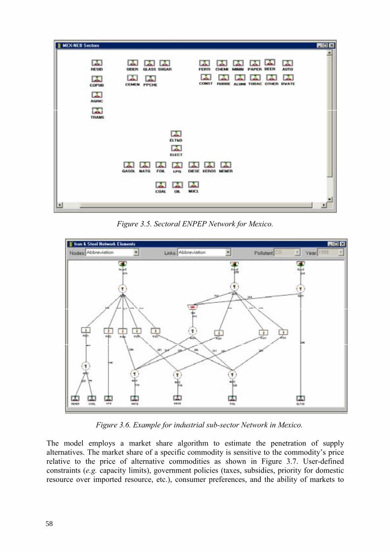
Figure 3.5. Sectoral ENPEP Network for Mexico.

Figure 3.6. Example for industrial sub-sector Network in Mexico.

The model employs a market share algorithm to estimate the penetration of supply alternatives. The market share of a specific commodity is sensitive to the commodity’s price relative to the price of alternative commodities as shown in Figure 3.7. User-defined constraints (e.g. capacity limits), government policies (taxes, subsidies, priority for domestic resource over imported resource, etc.), consumer preferences, and the ability of markets to

58

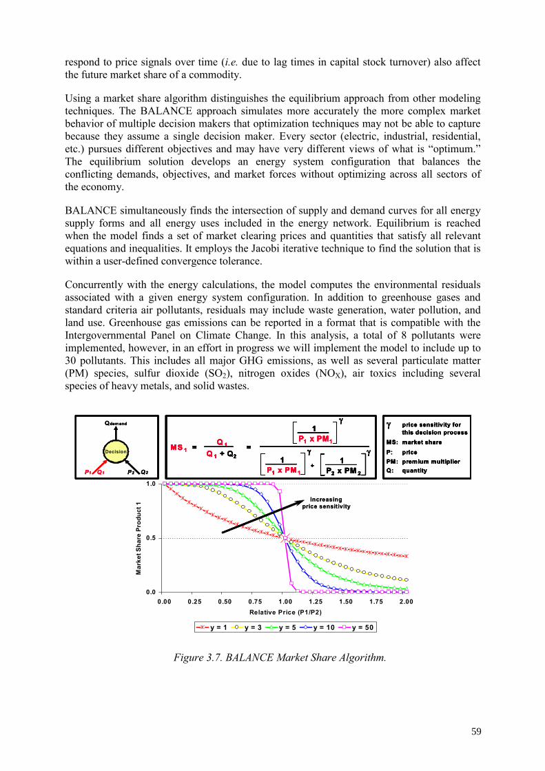
respond to price signals over time (i.e. due to lag times in capital stock turnover) also affect the future market share of a commodity.

Using a market share algorithm distinguishes the equilibrium approach from other modeling techniques. The BALANCE approach simulates more accurately the more complex market behavior of multiple decision makers that optimization techniques may not be able to capture because they assume a single decision maker. Every sector (electric, industrial, residential, etc.) pursues different objectives and may have very different views of what is “optimum.” The equilibrium solution develops an energy system configuration that balances the conflicting demands, objectives, and market forces without optimizing across all sectors of the economy.

BALANCE simultaneously finds the intersection of supply and demand curves for all energy supply forms and all energy uses included in the energy network. Equilibrium is reached when the model finds a set of market clearing prices and quantities that satisfy all relevant equations and inequalities. It employs the Jacobi iterative technique to find the solution that is within a user-defined convergence tolerance.

Concurrently with the energy calculations, the model computes the environmental residuals associated with a given energy system configuration. In addition to greenhouse gases and standard criteria air pollutants, residuals may include waste generation, water pollution, and land use. Greenhouse gas emissions can be reported in a format that is compatible with the Intergovernmental Panel on Climate Change. In this analysis, a total of 8 pollutants were implemented, however, in an effort in progress we will implement the model to include up to 30 pollutants. This includes all major GHG emissions, as well as several particulate matter (PM) species, sulfur dioxide (SO2), nitrogen oxides (NOX), air toxics including several species of heavy metals, and solid wastes.

0.0

0.5

1.0

0.00 0.25 0.50 0.75 1.00 1.25 1.50 1.75 2.00Relative Price (P1/P2)

Mar

ket S

hare

Pro

duct

1

y = 1 y = 3 y = 5 y = 10 y = 50

Increasingprice sensitivity

Increasingprice sensitivity

γ price sensitivity forthis decision process

MS: market shareP: pricePM:Q: quantity

premium multiplier

MS 1 =Q 1

Q 1 + Q2=

1P1 x PM1

γ

+1

P1 x PM 1

γ1

P2 x PM 2

γDecision

P1 Q1 P2 Q2

Qdemand γ price sensitivity forthis decision process


premium multiplier



premium multiplier



premium multiplier

MS 1 =Q 1

Q 1 + Q2=

1P1 x PM1

γ

+1

P1 x PM 1

γ1

P2 x PM 2

γMS 1 =Q 1

Q 1 + Q2=

1P1 x PM1

γ

+1

P1 x PM 1

γ1

P2 x PM 2

γMS 1 =Q 1

Q 1 + Q2=MS 1 =

Q 1

Q 1 + Q2=

1P1 x PM1

γ1

P1 x PM1

γ

+1

P1 x PM 1

γ1

P1 x PM 1

γ1

P2 x PM 2

γ1

P2 x PM 2

γDecision

P1 Q1 P2 Q2

Qdemand

Decision

P1 Q1 P2 Q2

Qdemand

Figure 3.7. BALANCE Market Share Algorithm.

59

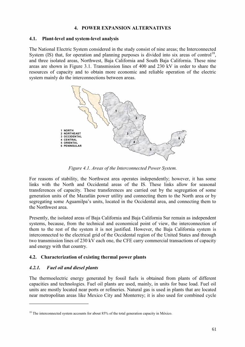
4. POWER EXPANSION ALTERNATIVES

4.1. Plant-level and system-level analysis

The National Electric System considered in the study consist of nine areas; the Interconnected System (IS) that, for operation and planning purposes is divided into six areas of control18, and three isolated areas, Northwest, Baja California and South Baja California. These nine areas are shown in Figure 3.1. Transmission lines of 400 and 230 kV in order to share the resources of capacity and to obtain more economic and reliable operation of the electric system mainly do the interconnections between areas.

11

22

3 3

44

55

66

1 NORTH2 NORTHEAST3 OCCIDENTAL4 CENTRAL5 ORIENTAL6 PENINSULAR

Figure 4.1. Areas of the Interconnected Power System.

For reasons of stability, the Northwest area operates independently; however, it has some links with the North and Occidental areas of the IS. These links allow for seasonal transferences of capacity. These transferences are carried out by the segregation of some generation units of the Mazatlán power utility and connecting them to the North area or by segregating some Aguamilpa’s units, located in the Occidental area, and connecting them to the Northwest area.

Presently, the isolated areas of Baja California and Baja California Sur remain as independent systems, because, from the technical and economical point of view, the interconnection of them to the rest of the system it is not justified. However, the Baja California system is interconnected to the electrical grid of the Occidental region of the United States and through two transmission lines of 230 kV each one, the CFE carry commercial transactions of capacity and energy with that country.

4.2. Characterization of existing thermal power plants

4.2.1. Fuel oil and diesel plants

The thermoelectric energy generated by fossil fuels is obtained from plants of different capacities and technologies. Fuel oil plants are used, mainly, in units for base load. Fuel oil units are mostly located near ports or refineries. Natural gas is used in plants that are located near metropolitan areas like Mexico City and Monterrey; it is also used for combined cycle

18 The interconnected system accounts for about 85% of the total generation capacity in México.

61

units. Diesel is used in plants that can operate during peak load periods. Among the main fuel oil plants are Manzanillo (1 900 MW) and Tuxpan (2,100 MW). Among the combined cycle plants an important one is Samalayuca II with a capacity of 521.7 MW.

4.2.2. Coal plants

Coal development is located in the state of Coahuila in the north of the country and comprises Rio Escondido plant with 1,200 MW, and Carbon II, with 1,400 MW.

4.2.3. Dual plants

Petacalco’s plant is a coal plant with 2,100 MW of capacity, it has the flexibility to use fuel oil and/or coal and it is located in Guerrero State.

4.2.4. Nuclear power plant

The nuclear power plant of Laguna Verde is located in the state of Veracruz. The first unit of 654.5 MW started operation in 1990; the second one, also of 654.5 MW, started operation in 1995. Presently, the capacity of each unit is 679 MW.

4.2.5. Geothermal plants

Geothermal energy in the Interconnected System is only 17.3% of the total geothermal capacity in the country. The geothermal power plants are located in Los Azufres with 87.9 MW and Los Humeros with 42 MW.

4.2.6. Wind plants

Wind energy in the Interconnected System is a very small fraction of the total capacity in the country. The wind power plants are located in La Venta, state of Oaxaca, with 1.575 MW. The rest of the wind power capacity is located in the isolated area of Baja California Sur in the location known as Guerrero Negro with a capacity of 0.6 MW.

4.3. Engineering data of the power technologies

Table 4.1 shows the grouping of the power stations by fuel type and their associated technical parameters. The net heat rate value for each technology, in both, the fixed system and the expansion of the power sector, are taken from the COPAR of CFE. On the basis of the heating value the specific consumption is calculated.

4.3.1. Emission factors

According to the Mexican ecological standard (NOM-085-ECOL-1994), for power units burning natural gas and fuel oil or diesel with different values for the sulfur content in the fuel the emission factors are shown in Table 4.2.For other fuels, on the basis of the % in weight of sulfur in the fuel (% S), the emission factor must be calculated by using the following equation19:

19 The equation is reported in the NOM-085-ECOL-1994 (Mexican Standard that regulates: smoke, total suspended

particulates, sulfur and nitrogen oxides from fixed sources that use fossil fuels).

62

=

×

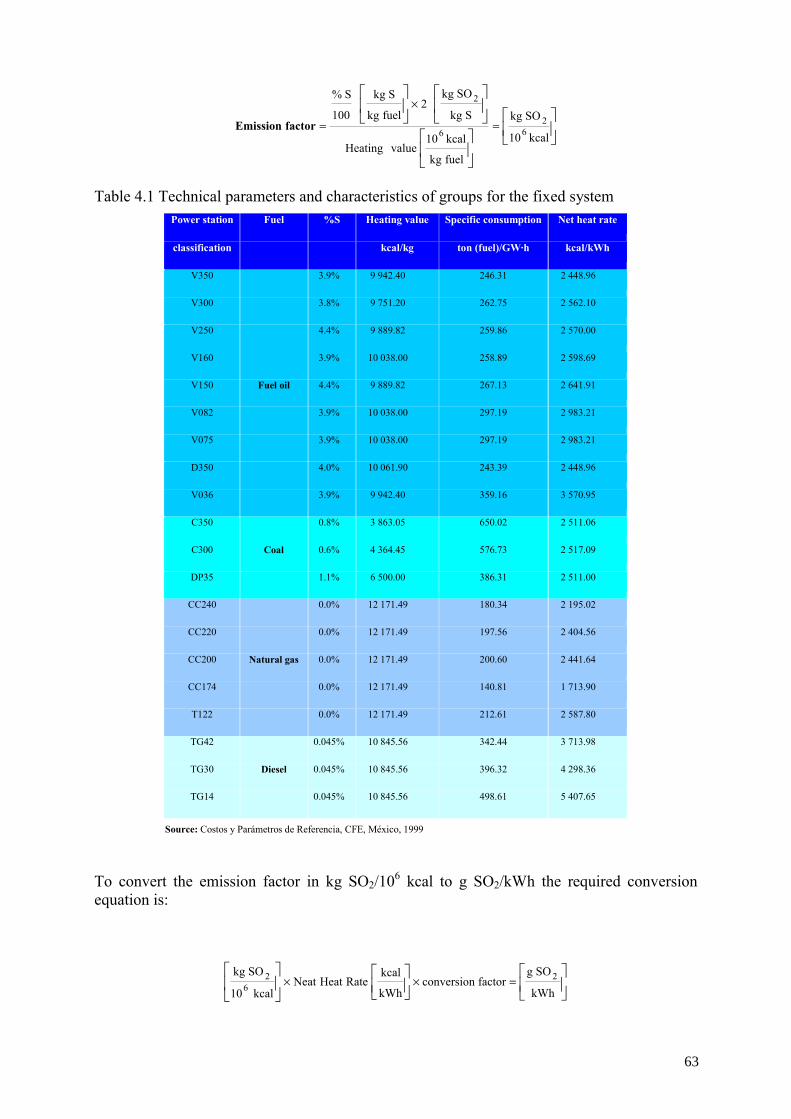
=kcal10

SOkg

fuelkg

kcal10valueHeating

Skg

SOkg2

fuelkg

Skg

100

S%

62

6

2

factorEmission

Table 4.1 Technical parameters and characteristics of groups for the fixed system Power station Fuel %S Heating value Specific consumption Net heat rate

classification kcal/kg ton (fuel)/GW·h kcal/kWh

V350 3.9% 9 942.40 246.31 2 448.96

V300 3.8% 9 751.20 262.75 2 562.10

V250 4.4% 9 889.82 259.86 2 570.00

V160 3.9% 10 038.00 258.89 2 598.69

V150 Fuel oil 4.4% 9 889.82 267.13 2 641.91

V082 3.9% 10 038.00 297.19 2 983.21

V075 3.9% 10 038.00 297.19 2 983.21

D350 4.0% 10 061.90 243.39 2 448.96

V036 3.9% 9 942.40 359.16 3 570.95

C350 0.8% 3 863.05 650.02 2 511.06

C300 Coal 0.6% 4 364.45 576.73 2 517.09

DP35 1.1% 6 500.00 386.31 2 511.00

CC240 0.0% 12 171.49 180.34 2 195.02

CC220 0.0% 12 171.49 197.56 2 404.56

CC200 Natural gas 0.0% 12 171.49 200.60 2 441.64

CC174 0.0% 12 171.49 140.81 1 713.90

T122 0.0% 12 171.49 212.61 2 587.80

TG42 0.045% 10 845.56 342.44 3 713.98

TG30 Diesel 0.045% 10 845.56 396.32 4 298.36

TG14 0.045% 10 845.56 498.61 5 407.65

Source: Costos y Parámetros de Referencia, CFE, México, 1999

To convert the emission factor in kg SO2/106 kcal to g SO2/kWh the required conversion equation is:

=××

kWh

SOgfactorconversion

kWh

kcalRateHeatNeat

kcal10

SOkg 26

2

63

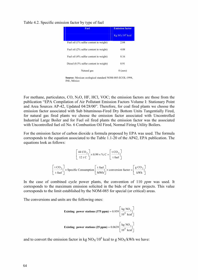
Table 4.2. Specific emission factor by type of fuel Fuel Emission factor

Kg SO2/106 kcal

Fuel oil (1% sulfur content in weight) 2.04



Diesel (0.5% sulfur content in weight) 0.91

Natural gas 0 (zero)

Source: Mexican ecological standard NOM-085-ECOL-1994, INE, México

For methane, particulates, CO, N2O, HF, HCl, VOC; the emission factors are those from the publication “EPA Compilation of Air Pollutant Emission Factors Volume I: Stationary Point and Area Sources AP-42, Updated 04/28/00”. Therefore, for coal fired plants we choose the emission factor associated with Sub bituminous-Fired Dry Bottom Units Tangentially Fired, for natural gas fired plants we choose the emission factor associated with Uncontrolled Industrial Large Boiler and for Fuel oil fired plants the emission factor was the associated with Uncontrolled fuel oil No. 6 Combustion Oil Fired, Normal Firing Utility Boilers.

For the emission factor of carbon dioxide a formula proposed by EPA was used. The formula corresponds to the equation associated to the Table 1.1-20 of the AP42, EPA publication. The equations look as follows:

=××

fuelt

COtC%99.0

Ct12

CO44 22

=××

kWh

COgfactorconversion

MWh

fueltnConsumptioSpecific

fuelt

COt 22

In the case of combined cycle power plants, the convention of 110 ppm was used. It corresponds to the maximum emission solicited in the bids of the new projects. This value corresponds to the limit established by the NOM-085 for special (or critical) areas.

The conversions and units are the following ones:

=

kcal10

NOkg0.959 6

xppm)(375stationspowerExisting

=

kcal10

NOkg0.0639 6

xppm)(25stationspowerExisting

and to convert the emission factor in kg NOX/106 kcal to g NOX/kWh we have:

64

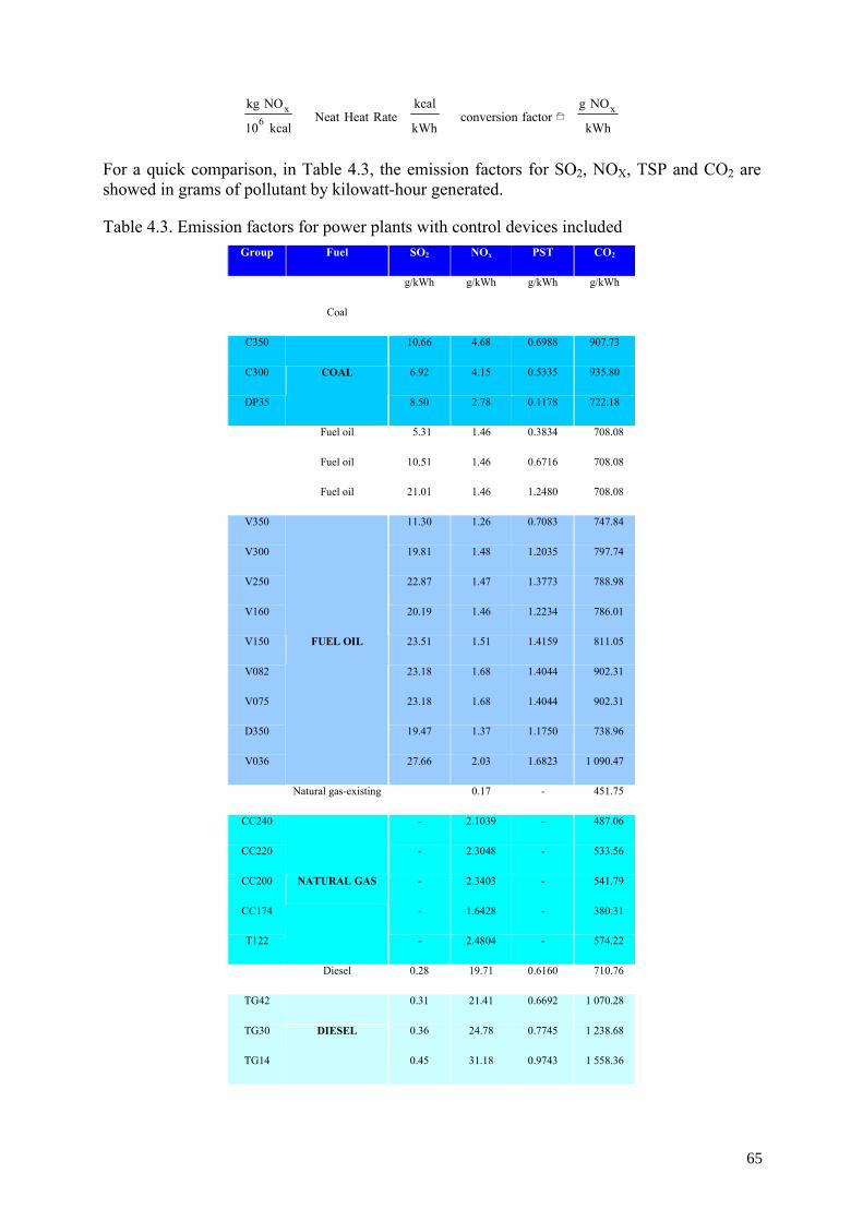
=��kWh

NOgfactorconversion

kWh

kcalRateHeatNeat

kcal10

NOkg x6

x

For a quick comparison, in Table 4.3, the emission factors for SO2, NOX, TSP and CO2 are showed in grams of pollutant by kilowatt-hour generated.

Table 4.3. Emission factors for power plants with control devices included Group Fuel SO2 NOx PST CO2

g/kWh g/kWh g/kWh g/kWh

Coal

C350 10.66 4.68 0.6988 907.73

C300 6.92 4.15 0.5335 935.80

DP35

COAL

8.50 2.78 0.1178 722.18

Fuel oil 5.31 1.46 0.3834 708.08

Fuel oil 10.51 1.46 0.6716 708.08

Fuel oil 21.01 1.46 1.2480 708.08

V350 11.30 1.26 0.7083 747.84

V300 19.81 1.48 1.2035 797.74

V250 22.87 1.47 1.3773 788.98

V160 20.19 1.46 1.2234 786.01

V150 23.51 1.51 1.4159 811.05

V082 23.18 1.68 1.4044 902.31

V075 23.18 1.68 1.4044 902.31

D350 19.47 1.37 1.1750 738.96

V036

FUEL OIL

27.66 2.03 1.6823 1 090.47

Natural gas-existing 0.17 - 451.75

CC240 - 2.1039 - 487.06

CC220 - 2.3048 - 533.56

CC200 - 2.3403 - 541.79

CC174 - 1.6428 - 380.31

T122

NATURAL GAS

- 2.4804 - 574.22

Diesel 0.28 19.71 0.6160 710.76

TG42 0.31 21.41 0.6692 1 070.28

TG30 0.36 24.78 0.7745 1 238.68

TG14

DIESEL

0.45 31.18 0.9743 1 558.36

65

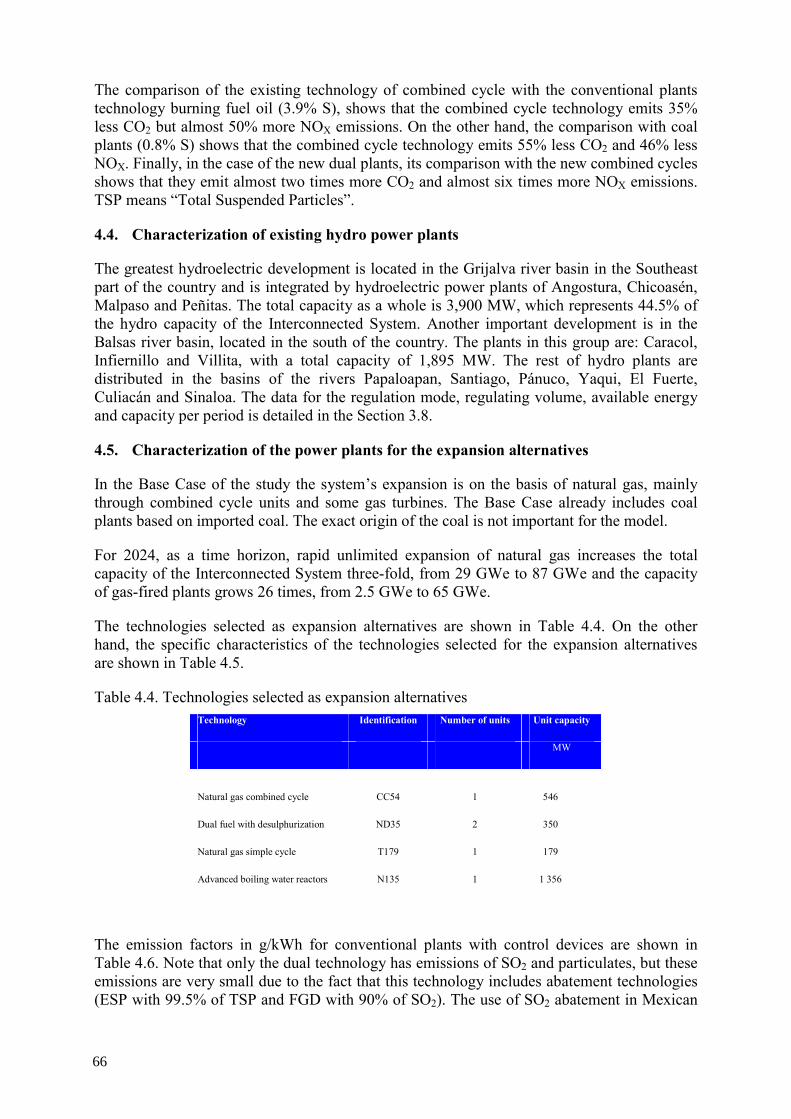
The comparison of the existing technology of combined cycle with the conventional plants technology burning fuel oil (3.9% S), shows that the combined cycle technology emits 35% less CO2 but almost 50% more NOX emissions. On the other hand, the comparison with coal plants (0.8% S) shows that the combined cycle technology emits 55% less CO2 and 46% less NOX. Finally, in the case of the new dual plants, its comparison with the new combined cycles shows that they emit almost two times more CO2 and almost six times more NOX emissions. TSP means “Total Suspended Particles”.

4.4. Characterization of existing hydro power plants

The greatest hydroelectric development is located in the Grijalva river basin in the Southeast part of the country and is integrated by hydroelectric power plants of Angostura, Chicoasén, Malpaso and Peñitas. The total capacity as a whole is 3,900 MW, which represents 44.5% of the hydro capacity of the Interconnected System. Another important development is in the Balsas river basin, located in the south of the country. The plants in this group are: Caracol, Infiernillo and Villita, with a total capacity of 1,895 MW. The rest of hydro plants are distributed in the basins of the rivers Papaloapan, Santiago, Pánuco, Yaqui, El Fuerte, Culiacán and Sinaloa. The data for the regulation mode, regulating volume, available energy and capacity per period is detailed in the Section 3.8.

4.5. Characterization of the power plants for the expansion alternatives

In the Base Case of the study the system’s expansion is on the basis of natural gas, mainly through combined cycle units and some gas turbines. The Base Case already includes coal plants based on imported coal. The exact origin of the coal is not important for the model.

For 2024, as a time horizon, rapid unlimited expansion of natural gas increases the total capacity of the Interconnected System three-fold, from 29 GWe to 87 GWe and the capacity of gas-fired plants grows 26 times, from 2.5 GWe to 65 GWe.

The technologies selected as expansion alternatives are shown in Table 4.4. On the other hand, the specific characteristics of the technologies selected for the expansion alternatives are shown in Table 4.5.

Table 4.4. Technologies selected as expansion alternatives Technology Identification Number of units Unit capacity

MW

Natural gas combined cycle CC54 1 546

Dual fuel with desulphurization ND35 2 350

Natural gas simple cycle T179 1 179

Advanced boiling water reactors N135 1 1 356

The emission factors in g/kWh for conventional plants with control devices are shown in Table 4.6. Note that only the dual technology has emissions of SO2 and particulates, but these emissions are very small due to the fact that this technology includes abatement technologies (ESP with 99.5% of TSP and FGD with 90% of SO2). The use of SO2 abatement in Mexican

66

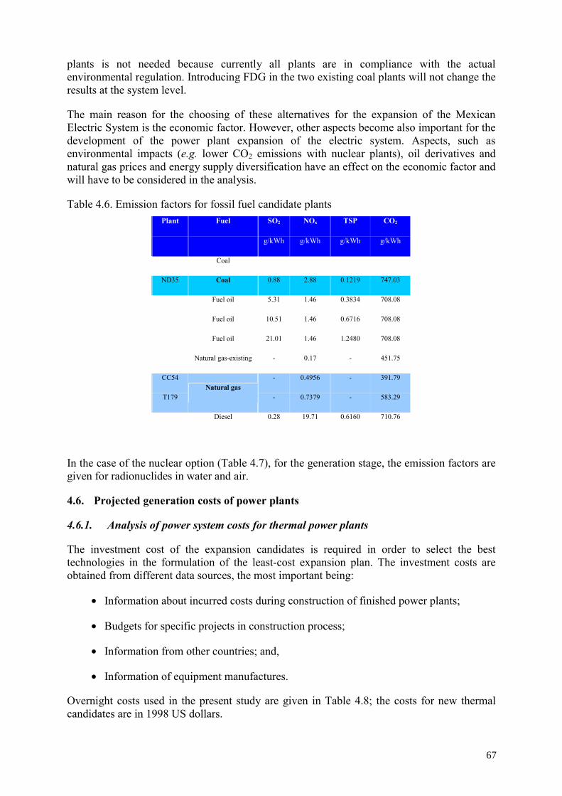
plants is not needed because currently all plants are in compliance with the actual environmental regulation. Introducing FDG in the two existing coal plants will not change the results at the system level.

The main reason for the choosing of these alternatives for the expansion of the Mexican Electric System is the economic factor. However, other aspects become also important for the development of the power plant expansion of the electric system. Aspects, such as environmental impacts (e.g. lower CO2 emissions with nuclear plants), oil derivatives and natural gas prices and energy supply diversification have an effect on the economic factor and will have to be considered in the analysis.

Table 4.6. Emission factors for fossil fuel candidate plants Plant Fuel SO2 NOx TSP CO2

g/kWh g/kWh g/kWh g/kWh

Coal

ND35 Coal 0.88 2.88 0.1219 747.03

Fuel oil 5.31 1.46 0.3834 708.08

Fuel oil 10.51 1.46 0.6716 708.08

Fuel oil 21.01 1.46 1.2480 708.08

Natural gas-existing - 0.17 - 451.75

CC54 - 0.4956 - 391.79

T179 Natural gas

- 0.7379 - 583.29

Diesel 0.28 19.71 0.6160 710.76

In the case of the nuclear option (Table 4.7), for the generation stage, the emission factors are given for radionuclides in water and air.

4.6. Projected generation costs of power plants

4.6.1. Analysis of power system costs for thermal power plants

The investment cost of the expansion candidates is required in order to select the best technologies in the formulation of the least-cost expansion plan. The investment costs are obtained from different data sources, the most important being:

• Information about incurred costs during construction of finished power plants;

• Budgets for specific projects in construction process;

• Information from other countries; and,

• Information of equipment manufactures.

Overnight costs used in the present study are given in Table 4.8; the costs for new thermal candidates are in 1998 US dollars.

67

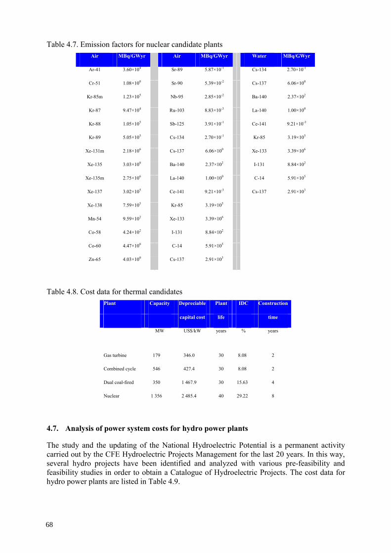
Table 4.7. Emission factors for nuclear candidate plants Air MBq/GWyr Air MBq/GWyr Water MBq/GWyr

Ar-41 3.60×104 Sr-89 5.87×10-1 Cs-134 2.70×10-1

Cr-51 1.08×100 Sr-90 5.39×10-2 Cs-137 6.06×100

Kr-85m 1.23×105 Nb-95 2.85×10-2 Ba-140 2.37×102

Kr-87 9.47×104 Ru-103 8.83×10-3 La-140 1.00×100

Kr-88 1.05×105 Sb-125 3.91×10-1 Ce-141 9.21×10-3

Kr-89 5.05×105 Cs-134 2.70×10-1 Kr-85 3.19×105

Xe-131m 2.18×106 Cs-137 6.06×100 Xe-133 3.39×106

Xe-135 3.03×108 Ba-140 2.37×102 I-131 8.84×102

Xe-135m 2.75×106 La-140 1.00×100 C-14 5.91×105

Xe-137 3.02×105 Ce-141 9.21×10-3 Cs-137 2.91×103

Xe-138 7.59×105 Kr-85 3.19×105

Mn-54 9.59×102 Xe-133 3.39×106

Co-58 4.24×102 I-131 8.84×102

Co-60 4.47×100 C-14 5.91×105

Zn-65 4.03×100 Cs-137 2.91×103

Table 4.8. Cost data for thermal candidates Plant Capacity Depreciable Plant IDC Construction

capital cost life time

MW US$/kW years % years

Gas turbine 179 346.0 30 8.08 2

Combined cycle 546 427.4 30 8.08 2

Dual coal-fired 350 1 467.9 30 15.63 4

Nuclear 1 356 2 485.4 40 29.22 8

4.7. Analysis of power system costs for hydro power plants

The study and the updating of the National Hydroelectric Potential is a permanent activity carried out by the CFE Hydroelectric Projects Management for the last 20 years. In this way, several hydro projects have been identified and analyzed with various pre-feasibility and feasibility studies in order to obtain a Catalogue of Hydroelectric Projects. The cost data for hydro power plants are listed in Table 4.9.

68

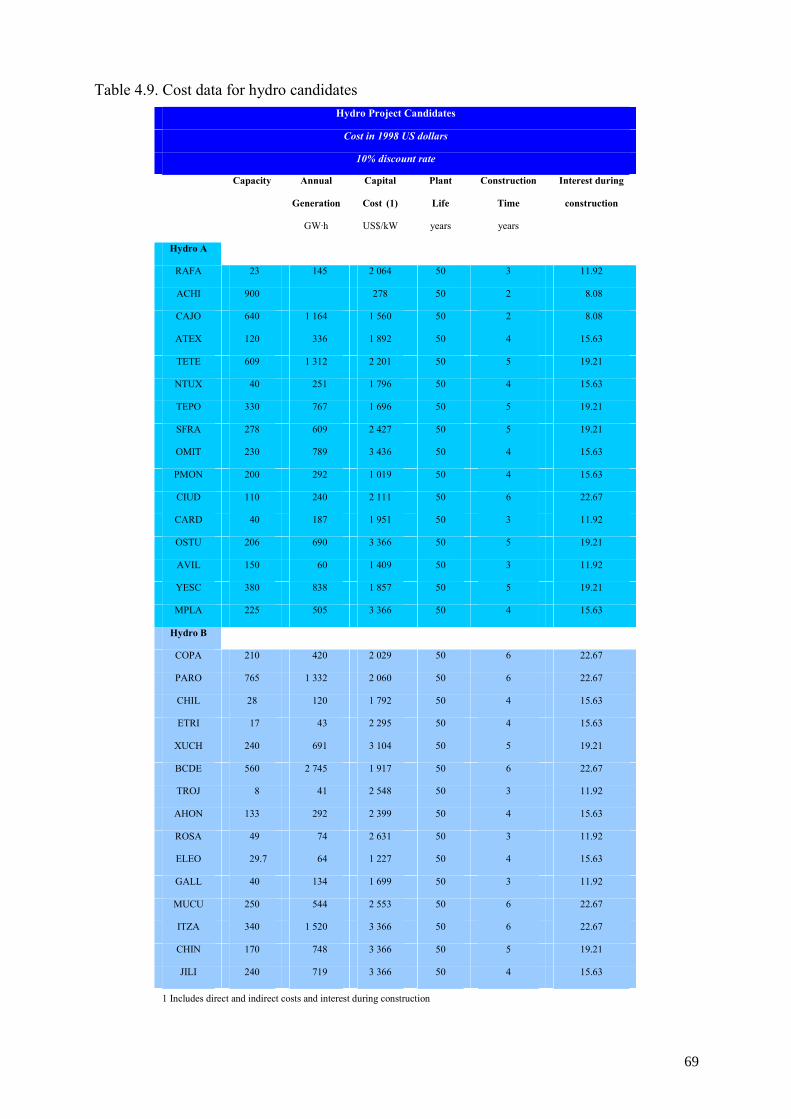
Table 4.9. Cost data for hydro candidates Hydro Project Candidates

Cost in 1998 US dollars

10% discount rate

Capacity Annual Capital Plant Construction Interest during

Generation Cost (1) Life Time construction

GW·h US$/kW years years

Hydro A

RAFA 23 145 2 064 50 3 11.92

ACHI 900 278 50 2 8.08

CAJO 640 1 164 1 560 50 2 8.08

ATEX 120 336 1 892 50 4 15.63

TETE 609 1 312 2 201 50 5 19.21

NTUX 40 251 1 796 50 4 15.63

TEPO 330 767 1 696 50 5 19.21

SFRA 278 609 2 427 50 5 19.21

OMIT 230 789 3 436 50 4 15.63

PMON 200 292 1 019 50 4 15.63

CIUD 110 240 2 111 50 6 22.67

CARD 40 187 1 951 50 3 11.92

OSTU 206 690 3 366 50 5 19.21

AVIL 150 60 1 409 50 3 11.92

YESC 380 838 1 857 50 5 19.21

MPLA 225 505 3 366 50 4 15.63

Hydro B

COPA 210 420 2 029 50 6 22.67

PARO 765 1 332 2 060 50 6 22.67

CHIL 28 120 1 792 50 4 15.63

ETRI 17 43 2 295 50 4 15.63

XUCH 240 691 3 104 50 5 19.21

BCDE 560 2 745 1 917 50 6 22.67

TROJ 8 41 2 548 50 3 11.92

AHON 133 292 2 399 50 4 15.63

ROSA 49 74 2 631 50 3 11.92

ELEO 29.7 64 1 227 50 4 15.63

GALL 40 134 1 699 50 3 11.92

MUCU 250 544 2 553 50 6 22.67

ITZA 340 1 520 3 366 50 6 22.67

CHIN 170 748 3 366 50 5 19.21

JILI 240 719 3 366 50 4 15.63

1 Includes direct and indirect costs and interest during construction

69

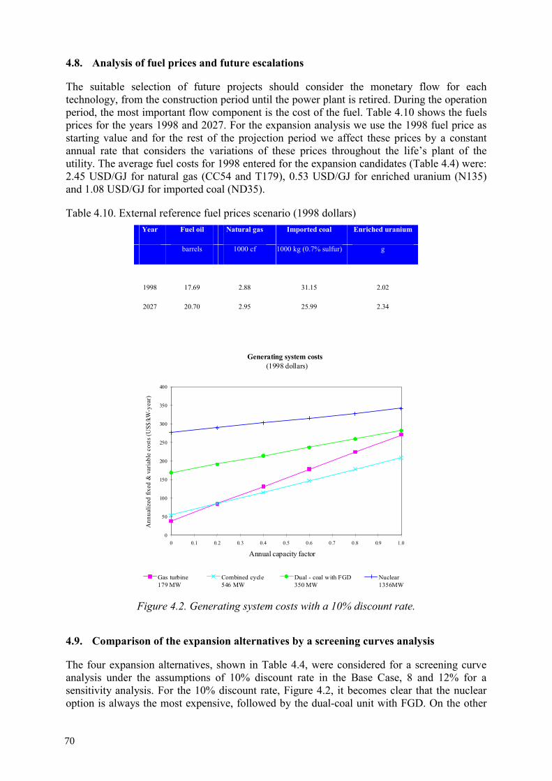
4.8. Analysis of fuel prices and future escalations

The suitable selection of future projects should consider the monetary flow for each technology, from the construction period until the power plant is retired. During the operation period, the most important flow component is the cost of the fuel. Table 4.10 shows the fuels prices for the years 1998 and 2027. For the expansion analysis we use the 1998 fuel price as starting value and for the rest of the projection period we affect these prices by a constant annual rate that considers the variations of these prices throughout the life’s plant of the utility. The average fuel costs for 1998 entered for the expansion candidates (Table 4.4) were: 2.45 USD/GJ for natural gas (CC54 and T179), 0.53 USD/GJ for enriched uranium (N135) and 1.08 USD/GJ for imported coal (ND35).

Table 4.10. External reference fuel prices scenario (1998 dollars) Year Fuel oil Natural gas Imported coal Enriched uranium

barrels 1000 cf 1000 kg (0.7% sulfur) g

1998 17.69 2.88 31.15 2.02

2027 20.70 2.95 25.99 2.34

Generating system costs

(1998 dollars)

0

50

100

150

200

250

300

350

400

0 0.1 0.2 0.3 0.4 0.5 0.6 0.7 0.8 0.9 1.0 Annual capacity factor

Ann

ualiz

ed fi

xed

& v

aria

ble

cost

s (U

S$/k

W-y

ear)

Gas turbine 179 MW

Combined cycle 546 MW

Dual - coal with FGD 350 MW

Nuclear 1356MW

Figure 4.2. Generating system costs with a 10% discount rate.

4.9. Comparison of the expansion alternatives by a screening curves analysis

The four expansion alternatives, shown in Table 4.4, were considered for a screening curve analysis under the assumptions of 10% discount rate in the Base Case, 8 and 12% for a sensitivity analysis. For the 10% discount rate, Figure 4.2, it becomes clear that the nuclear option is always the most expensive, followed by the dual-coal unit with FGD. On the other

70

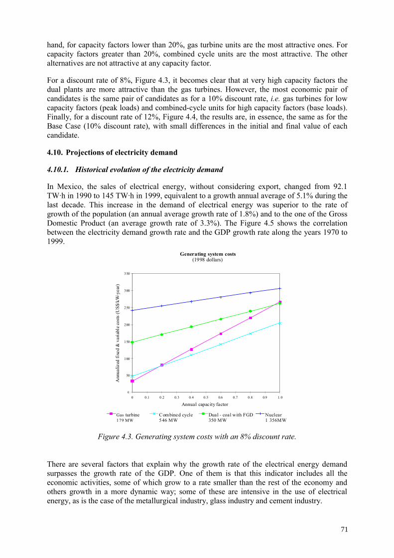
hand, for capacity factors lower than 20%, gas turbine units are the most attractive ones. For capacity factors greater than 20%, combined cycle units are the most attractive. The other alternatives are not attractive at any capacity factor.

For a discount rate of 8%, Figure 4.3, it becomes clear that at very high capacity factors the dual plants are more attractive than the gas turbines. However, the most economic pair of candidates is the same pair of candidates as for a 10% discount rate, i.e. gas turbines for low capacity factors (peak loads) and combined-cycle units for high capacity factors (base loads). Finally, for a discount rate of 12%, Figure 4.4, the results are, in essence, the same as for the Base Case (10% discount rate), with small differences in the initial and final value of each candidate.

4.10. Projections of electricity demand

4.10.1. Historical evolution of the electricity demand

In Mexico, the sales of electrical energy, without considering export, changed from 92.1 TW·h in 1990 to 145 TW·h in 1999, equivalent to a growth annual average of 5.1% during the last decade. This increase in the demand of electrical energy was superior to the rate of growth of the population (an annual average growth rate of 1.8%) and to the one of the Gross Domestic Product (an average growth rate of 3.3%). The Figure 4.5 shows the correlation between the electricity demand growth rate and the GDP growth rate along the years 1970 to 1999.

Generating system costs(1998 dollars)

0

50

100

150

200

250

300

350

0 0.1 0.2 0.3 0.4 0.5 0.6 0.7 0.8 0.9 1.0

Annual capacity factor

Ann

ualiz

ed fi

xed

& v

aria

ble

costs

(US$

/kW

-yea

r)

Gas turbine 179 MW

Combined cycle546 MW

Dual - coal with FGD350 MW

Nuclear 1 356MW

Figure 4.3. Generating system costs with an 8% discount rate.

There are several factors that explain why the growth rate of the electrical energy demand surpasses the growth rate of the GDP. One of them is that this indicator includes all the economic activities, some of which grow to a rate smaller than the rest of the economy and others growth in a more dynamic way; some of these are intensive in the use of electrical energy, as is the case of the metallurgical industry, glass industry and cement industry.

71

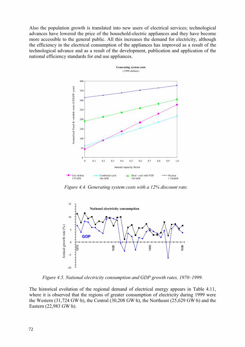
Also the population growth is translated into new users of electrical services; technological advances have lowered the price of the household-electric appliances and they have become more accessible to the general public. All this increases the demand for electricity, although the efficiency in the electrical consumption of the appliances has improved as a result of the technological advance and as a result of the development, publication and application of the national efficiency standards for end use appliances.

Generating system costs

(1998 dollars)

0

50

100

150

200

250

300

350

400

0 0.1 0.2 0.3 0.4 0.5 0.6 0.7 0.8 0.9 1.0


Ann

ualiz

ed fi

xed

& v

aria

ble

cost

s (U

S$/k

W-y

ear)

Gas turbine 179 MW

Combined cycle546 MW

Dual - coal with FGD350 MW

Nuclear 1 356MW

Figure 4.4. Generating system costs with a 12% discount rate.

Ann

ual g

row

th ra

te (%

)

0

5

10

15

-5

-10

1970

1980

1990

1999

GDP

National electricity consumption

Figure 4.5. National electricity consumption and GDP growth rates, 1970–1999.

The historical evolution of the regional demand of electrical energy appears in Table 4.11, where it is observed that the regions of greater consumption of electricity during 1999 were the Western (31,724 GW·h), the Central (30,208 GW·h), the Northeast (25,629 GW·h) and the Eastern (22,983 GW·h).

72

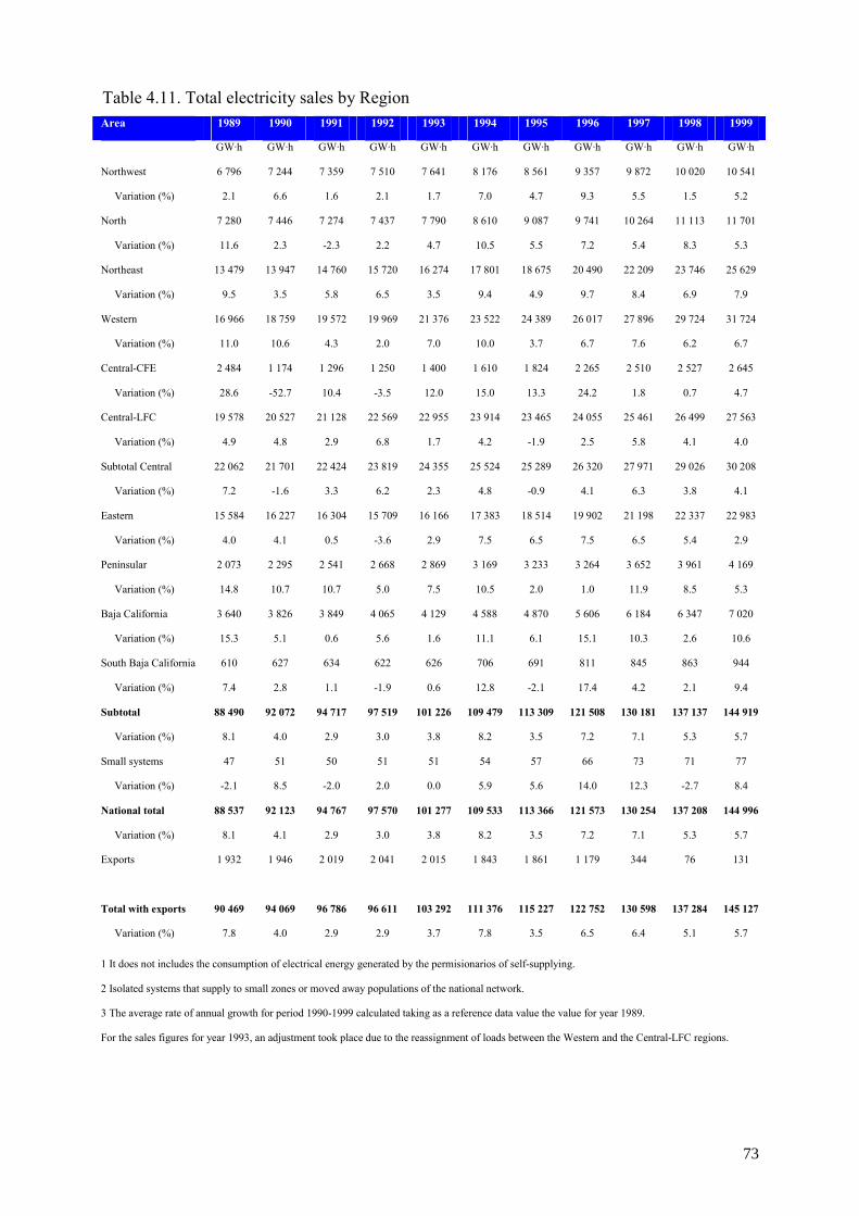
Table 4.11. Total electricity sales by Region Area 1989 1990 1991 1992 1993 1994 1995 1996 1997 1998 1999

GW·h GW·h GW·h GW·h GW·h GW·h GW·h GW·h GW·h GW·h GW·h

Northwest 6 796 7 244 7 359 7 510 7 641 8 176 8 561 9 357 9 872 10 020 10 541

Variation (%) 2.1 6.6 1.6 2.1 1.7 7.0 4.7 9.3 5.5 1.5 5.2

North 7 280 7 446 7 274 7 437 7 790 8 610 9 087 9 741 10 264 11 113 11 701

Variation (%) 11.6 2.3 -2.3 2.2 4.7 10.5 5.5 7.2 5.4 8.3 5.3

Northeast 13 479 13 947 14 760 15 720 16 274 17 801 18 675 20 490 22 209 23 746 25 629

Variation (%) 9.5 3.5 5.8 6.5 3.5 9.4 4.9 9.7 8.4 6.9 7.9

Western 16 966 18 759 19 572 19 969 21 376 23 522 24 389 26 017 27 896 29 724 31 724

Variation (%) 11.0 10.6 4.3 2.0 7.0 10.0 3.7 6.7 7.6 6.2 6.7

Central-CFE 2 484 1 174 1 296 1 250 1 400 1 610 1 824 2 265 2 510 2 527 2 645

Variation (%) 28.6 -52.7 10.4 -3.5 12.0 15.0 13.3 24.2 1.8 0.7 4.7

Central-LFC 19 578 20 527 21 128 22 569 22 955 23 914 23 465 24 055 25 461 26 499 27 563

Variation (%) 4.9 4.8 2.9 6.8 1.7 4.2 -1.9 2.5 5.8 4.1 4.0

Subtotal Central 22 062 21 701 22 424 23 819 24 355 25 524 25 289 26 320 27 971 29 026 30 208

Variation (%) 7.2 -1.6 3.3 6.2 2.3 4.8 -0.9 4.1 6.3 3.8 4.1

Eastern 15 584 16 227 16 304 15 709 16 166 17 383 18 514 19 902 21 198 22 337 22 983

Variation (%) 4.0 4.1 0.5 -3.6 2.9 7.5 6.5 7.5 6.5 5.4 2.9

Peninsular 2 073 2 295 2 541 2 668 2 869 3 169 3 233 3 264 3 652 3 961 4 169

Variation (%) 14.8 10.7 10.7 5.0 7.5 10.5 2.0 1.0 11.9 8.5 5.3

Baja California 3 640 3 826 3 849 4 065 4 129 4 588 4 870 5 606 6 184 6 347 7 020

Variation (%) 15.3 5.1 0.6 5.6 1.6 11.1 6.1 15.1 10.3 2.6 10.6

South Baja California 610 627 634 622 626 706 691 811 845 863 944

Variation (%) 7.4 2.8 1.1 -1.9 0.6 12.8 -2.1 17.4 4.2 2.1 9.4

Subtotal 88 490 92 072 94 717 97 519 101 226 109 479 113 309 121 508 130 181 137 137 144 919

Variation (%) 8.1 4.0 2.9 3.0 3.8 8.2 3.5 7.2 7.1 5.3 5.7

Small systems 47 51 50 51 51 54 57 66 73 71 77

Variation (%) -2.1 8.5 -2.0 2.0 0.0 5.9 5.6 14.0 12.3 -2.7 8.4

National total 88 537 92 123 94 767 97 570 101 277 109 533 113 366 121 573 130 254 137 208 144 996

Variation (%) 8.1 4.1 2.9 3.0 3.8 8.2 3.5 7.2 7.1 5.3 5.7

Exports 1 932 1 946 2 019 2 041 2 015 1 843 1 861 1 179 344 76 131

Total with exports 90 469 94 069 96 786 96 611 103 292 111 376 115 227 122 752 130 598 137 284 145 127

Variation (%) 7.8 4.0 2.9 2.9 3.7 7.8 3.5 6.5 6.4 5.1 5.7

1 It does not includes the consumption of electrical energy generated by the permisionarios of self-supplying.

2 Isolated systems that supply to small zones or moved away populations of the national network.

3 The average rate of annual growth for period 1990-1999 calculated taking as a reference data value the value for year 1989.

For the sales figures for year 1993, an adjustment took place due to the reassignment of loads between the Western and the Central-LFC regions.

73

4.11. Historical system load factors and seasonal variation of peak load

The load of a system is constituted by a great number of individual loads of different classes (industrial, residential, commercial, etc.) and of small power with respect to the required total. The respective moments of connection and disconnection of these loads are random, but the required average power in a period given by the assembly of loads follows a certain pattern that depends on the rate of the human activities in the region supplied by the electrical system

Figure 4.6 shows typical average load curves for the areas of the north and the south of the country, corresponding to the working days and holidays for summer and the winter seasons of 1999. The relative magnitude of the hourly loads with respect to maximum annual demand of power is shown. It is possible to see that the load profiles depend on the geographic region, the season of the year and the working and holiday days. For example, it is observed that during the working days more electricity than in the holiday days is consumed. In the areas of the north of the country, during the summer the use of electrical energy is greater than during the winter and the peak of demand appears from 14 to 18 hours in the summer days. For the south areas we notice a slightly major consumption in the winter and the peak of the demand appears at the 20 hours in the winter days. The introduction of the hourly tariffs for the clients with larger demand has caused a change in its consumption patterns, which is reflected in the reduction of the growth rate of the peak’s demand, with the consequent benefit of a better handling of the generation capacity.

4.12. System reserve and reliability

In the planning of the additions of capacity of any electrical system it is necessary to take into account the reserve’s capacity that is required to guarantee reliability of the supply because:

• It is not feasible to store the electrical energy for later use, for this reason it is necessary to produce it at the moment it is required.

• The system’s capacity is subject to reductions as a result of programmed exits of the plants for maintenance and fortuitous events such as faults; degradation and other causes (dry hydrologic years, etc.).

In order to satisfy the demand in suitable conditions of reliability, the capacity of the electrical system must be greater than the annual maximum demand. The reserve capacity is the difference between the capacity of the system and the maximum demand within certain period (demand tip). The reserve margin it is defined as the difference between the capacity and the maximum demand in percent of the maximum demand.

The reserve capacity of an electrical system depends on the different types of power stations that conforms it and their availability factors, of the capacity of the generating units in relation to the total, and of the conditions of the interconnection. The requirements of capacity of the weakly interconnected isolated systems or to each other are determined on an individual way, based on their own maximum demand and load curves.

When several regional systems are interconnected reliably, it is possible to reduce the reserve margin, because the resources of generation capacity can be shared in a more efficient form between the different regions; in addition, the capacity requirements can be determined by the coincident maximum demand, which is minor than the sum of the maximum demands of the regional systems, since these happen at different moments within the year (are not chronologically coincident).

74

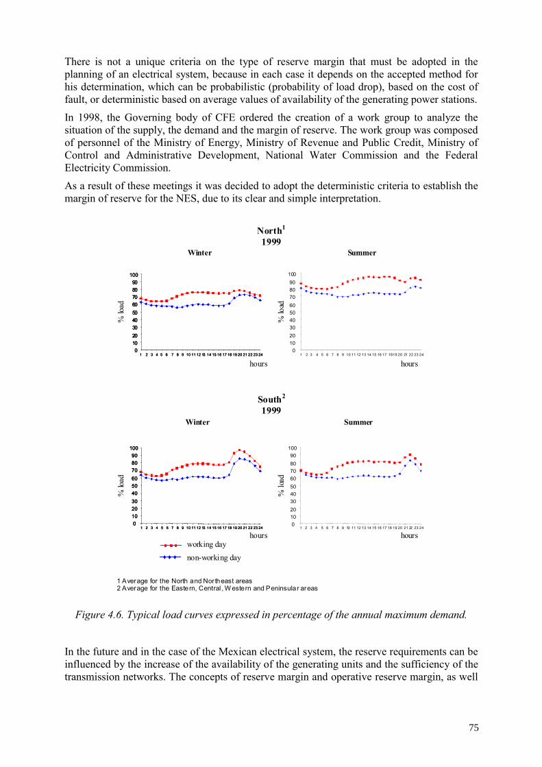
There is not a unique criteria on the type of reserve margin that must be adopted in the planning of an electrical system, because in each case it depends on the accepted method for his determination, which can be probabilistic (probability of load drop), based on the cost of fault, or deterministic based on average values of availability of the generating power stations.

In 1998, the Governing body of CFE ordered the creation of a work group to analyze the situation of the supply, the demand and the margin of reserve. The work group was composed of personnel of the Ministry of Energy, Ministry of Revenue and Public Credit, Ministry of Control and Administrative Development, National Water Commission and the Federal Electricity Commission.

As a result of these meetings it was decided to adopt the deterministic criteria to establish the margin of reserve for the NES, due to its clear and simple interpretation.

0 10 20 30 40 50 60 70 80 90 100

1 2 3 4 5 6 7 8 9 10 11 12 13 14 15 16 17 18 19 20 21 22 23 24

0 10 20 30 40 50 60 70 80 90 100

1 2 3 4 5 6 7 8 9 10 11 12 13 14 15 16 17 18 19 20 21 22 23 240

102030405060708090100

1 2 3 4 5 6 7 8 9 10 11 12 13 14 15 16 17 18 19 20 21 22 23 24

0102030405060708090

100

1 2 3 4 5 6 7 8 9 10 11 12 13 14 15 16 17 18 19 20 21 22 23 24

% lo

ad

hours hours

Winter Summer

% lo

ad

0 10 20 30 40 50 60 70 80 90 100

1 2 3 4 5 6 7 8 9 10 11 12 13 14 15 16 17 18 19 20 21 22 23 240 10 20 30 40 50 60 70 80 90 100

1 2 3 4 5 6 7 8 9 10 11 12 13 14 15 16 17 18 19 20 21 22 23 24

0 10 20 30 40 50 60 70 80 90 100

1 2 3 4 5 6 7 8 9 10 11 12 13 14 15 16 17 18 19 20 21 22 23 240 10 20

30 40 50 60 70 80 90 100

1 2 3 4 5 6 7 8 9 10 11 12 13 14 15 16 17 18 19 20 21 22 23 24

Winter Summer

North1

1999

South2

1999

working daynon-working day

% lo

ad

hours

% lo

ad

hours

1 Average for the North and Nor theast areas 2 Average for the Eastern, Central , W estern and Peninsular areas

Figure 4.6. Typical load curves expressed in percentage of the annual maximum demand.

In the future and in the case of the Mexican electrical system, the reserve requirements can be influenced by the increase of the availability of the generating units and the sufficiency of the transmission networks. The concepts of reserve margin and operative reserve margin, as well

75

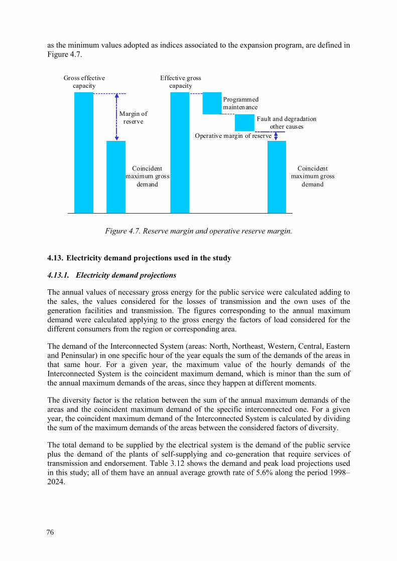
as the minimum values adopted as indices associated to the expansion program, are defined in Figure 4.7.

Margin of reserve

Gross effective capacity

Coincident maximum gross

demand

Coincident maximum gross

demand

Effective grosscapacity

Programmedmaintenance

Fault and degradation other causes

Operative margin of reserve

Figure 4.7. Reserve margin and operative reserve margin.

4.13. Electricity demand projections used in the study

4.13.1. Electricity demand projections

The annual values of necessary gross energy for the public service were calculated adding to the sales, the values considered for the losses of transmission and the own uses of the generation facilities and transmission. The figures corresponding to the annual maximum demand were calculated applying to the gross energy the factors of load considered for the different consumers from the region or corresponding area.

The demand of the Interconnected System (areas: North, Northeast, Western, Central, Eastern and Peninsular) in one specific hour of the year equals the sum of the demands of the areas in that same hour. For a given year, the maximum value of the hourly demands of the Interconnected System is the coincident maximum demand, which is minor than the sum of the annual maximum demands of the areas, since they happen at different moments.

The diversity factor is the relation between the sum of the annual maximum demands of the areas and the coincident maximum demand of the specific interconnected one. For a given year, the coincident maximum demand of the Interconnected System is calculated by dividing the sum of the maximum demands of the areas between the considered factors of diversity.

The total demand to be supplied by the electrical system is the demand of the public service plus the demand of the plants of self-supplying and co-generation that require services of transmission and endorsement. Table 3.12 shows the demand and peak load projections used in this study; all of them have an annual average growth rate of 5.6% along the period 1998–2024.

76

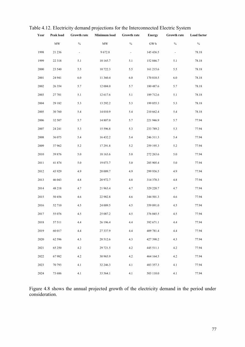
Table 4.12. Electricity demand projections for the Interconnected Electric System Year Peak load Growth rate Minimum load Growth rate Energy Growth rate Load factor

MW % MW % GW·h % %

1998 21 236 - 9 672.8 - 145 436.5 - 78.18

1999 22 318 5.1 10 165.7 5.1 152 846.7 5.1 78.18

2000 23 540 5.5 10 722.3 5.5 161 215.6 5.5 78.18

2001 24 941 6.0 11 360.4 6.0 170 810.5 6.0 78.18

2002 26 354 5.7 12 004.0 5.7 180 487.6 5.7 78.18

2003 27 701 5.1 12 617.6 5.1 189 712.6 5.1 78.18

2004 29 182 5.3 13 292.2 5.3 199 855.3 5.3 78.18

2005 30 760 5.4 14 010.9 5.4 210 662.4 5.4 78.18

2006 32 507 5.7 14 807.0 5.7 221 946.9 5.7 77.94

2007 24 241 5.3 15 596.8 5.3 233 789.2 5.3 77.94

2008 36 075 5.4 16 432.2 5.4 246 311.3 5.4 77.94

2009 37 962 5.2 17 291.8 5.2 259 195.3 5.2 77.94

2010 39 876 5.0 18 163.6 5.0 272 263.6 5.0 77.94

2011 41 874 5.0 19 073.7 5.0 285 905.4 5.0 77.94

2012 43 929 4.9 20 009.7 4.9 299 936.5 4.9 77.94

2013 46 043 4.8 20 972.7 4.8 314 370.3 4.8 77.94

2014 48 218 4.7 21 963.4 4.7 329 220.7 4.7 77.94

2015 50 456 4.6 22 982.8 4.6 344 501.3 4.6 77.94

2016 52 710 4.5 24 009.5 4.5 359 891.0 4.5 77.94

2017 55 076 4.5 25 087.2 4.5 376 045.5 4.5 77.94

2018 57 511 4.4 26 196.4 4.4 392 671.1 4.4 77.94

2019 60 017 4.4 27 337.9 4.4 409 781.4 4.4 77.94

2020 62 596 4.3 28 512.6 4.3 427 390.2 4.3 77.94

2021 65 250 4.2 29 721.5 4.2 445 511.1 4.2 77.94

2022 67 982 4.2 30 965.9 4.2 464 164.5 4.2 77.94

2023 70 793 4.1 32 246.3 4.1 483 357.3 4.1 77.94

2024 73 686 4.1 33 564.1 4.1 503 110.0 4.1 77.94

Figure 4.8 shows the annual projected growth of the electricity demand in the period under consideration.

77

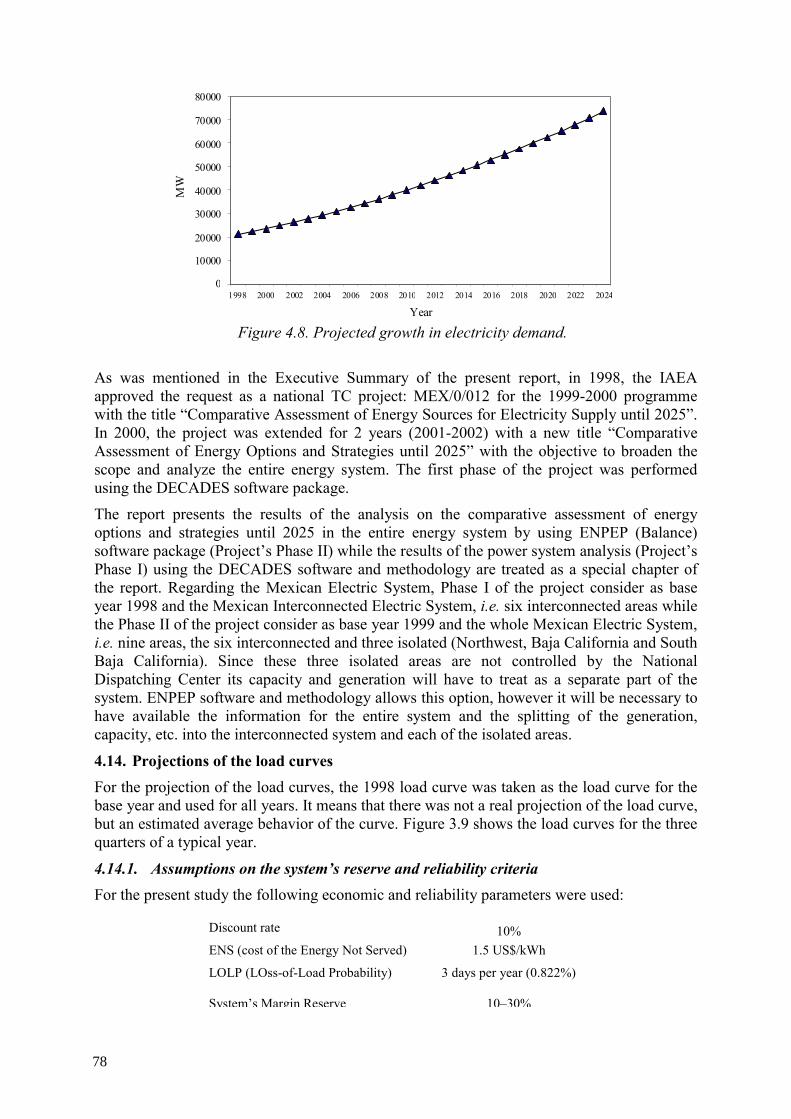
0

10000

20000

30000

40000

50000

60000

70000

80000

1998 2000 2002 2004 2006 2008 2010 2012 2014 2016 2018 2020 2022 2024

Year

MW

Figure 4.8. Projected growth in electricity demand.

As was mentioned in the Executive Summary of the present report, in 1998, the IAEA approved the request as a national TC project: MEX/0/012 for the 1999-2000 programme with the title “Comparative Assessment of Energy Sources for Electricity Supply until 2025”. In 2000, the project was extended for 2 years (2001-2002) with a new title “Comparative Assessment of Energy Options and Strategies until 2025” with the objective to broaden the scope and analyze the entire energy system. The first phase of the project was performed using the DECADES software package.

The report presents the results of the analysis on the comparative assessment of energy options and strategies until 2025 in the entire energy system by using ENPEP (Balance) software package (Project’s Phase II) while the results of the power system analysis (Project’s Phase I) using the DECADES software and methodology are treated as a special chapter of the report. Regarding the Mexican Electric System, Phase I of the project consider as base year 1998 and the Mexican Interconnected Electric System, i.e. six interconnected areas while the Phase II of the project consider as base year 1999 and the whole Mexican Electric System, i.e. nine areas, the six interconnected and three isolated (Northwest, Baja California and South Baja California). Since these three isolated areas are not controlled by the National Dispatching Center its capacity and generation will have to treat as a separate part of the system. ENPEP software and methodology allows this option, however it will be necessary to have available the information for the entire system and the splitting of the generation, capacity, etc. into the interconnected system and each of the isolated areas.

4.14. Projections of the load curves For the projection of the load curves, the 1998 load curve was taken as the load curve for the base year and used for all years. It means that there was not a real projection of the load curve, but an estimated average behavior of the curve. Figure 3.9 shows the load curves for the three quarters of a typical year.

4.14.1. Assumptions on the system’s reserve and reliability criteria For the present study the following economic and reliability parameters were used:

Discount rate 10% ENS (cost of the Energy Not Served) 1.5 US$/kWh

LOLP (LOss-of-Load Probability) 3 days per year (0.822%)

System’s Margin Reserve 10–30%

78

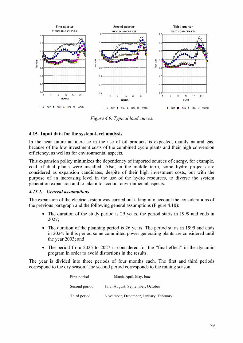
TIPIC LOAD CURVES

0.3 0.4

0.5 0.6

0.7

0.8

0.9 1.0

1 5 9 13 17 21 HOURS

SAT SUN HOL WORK

TIPIC LOAD CURVES

0.3

0.4

0.5

0.6

0.7

0.8

0.9

1.0

1 5 9 13 17 21

HOURS

SAT SUN HOL WORK

TIPIC LOAD CURVES

0.3

0.4

0.5

0.6

0.7

0.8

0.9

1.0

1 5 9 13 17 21

HOURS

SAT SUN HOL WORK

Free

uni

t

Free

uni

t

Free

uni

t

First quarter Second quarter Third quarter

Figure 4.9. Typical load curves.

4.15. Input data for the system-level analysis In the near future an increase in the use of oil products is expected, mainly natural gas, because of the low investment costs of the combined cycle plants and their high conversion efficiency, as well as for environmental aspects.

This expansion policy minimizes the dependency of imported sources of energy, for example, coal, if dual plants were installed. Also, in the middle term, some hydro projects are considered as expansion candidates, despite of their high investment costs, but with the purpose of an increasing level in the use of the hydro resources, to diverse the system generation expansion and to take into account environmental aspects.

4.15.1. General assumptions The expansion of the electric system was carried out taking into account the considerations of the previous paragraph and the following general assumptions (Figure 4.10):

• The duration of the study period is 29 years, the period starts in 1999 and ends in 2027;

• The duration of the planning period is 26 years. The period starts in 1999 and ends in 2024. In this period some committed power generating plants are considered until the year 2003; and

• The period from 2025 to 2027 is considered for the “final effect” in the dynamic program in order to avoid distortions in the results.

The year is divided into three periods of four months each. The first and third periods correspond to the dry season. The second period corresponds to the raining season.

First period March, April, May, June

Second period July, August, September, October

Third period November, December, January, February

79

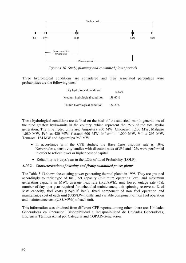
Study period

1998 1999 2003 2024 2027

Some committed power plants

Planning period Figure 4.10. Study, planning and committed plants periods.

Three hydrological conditions are considered and their associated percentage wise probabilities are the following ones:

Dry hydrological condition 19.06%

Medium hydrological condition 58.67%

Humid hydrological condition 22.27%

These hydrological conditions are defined on the basis of the statistical-month generations of the nine greatest hydro-units in the country, which represent the 75% of the total hydro generation. The nine hydro units are: Angostura 900 MW, Chicoasén 1,500 MW, Malpaso 1,080 MW, Peñitas 420 MW, Caracol 600 MW, Infiernillo 1,000 MW, Villita 295 MW, Temascal 154 MW and Aguamilpa 960 MW.

• In accordance with the CFE studies, the Base Case discount rate is 10%. Nevertheless, sensitivity studies with discount rates of 8% and 12% were performed in order to reflect lower or higher cost of capital.

• Reliability is 3 days/year in the LOss of Load Probability (LOLP).

4.15.2. Characterization of existing and firmly committed power plants

The Table 3.13 shows the existing power generating thermal plants in 1998. They are grouped accordingly to their type of fuel, net capacity (minimum operating level and maximum generating capacity in MW), average heat rate (kcal/kWh), unit forced outage rate (%), number of days per year required for scheduled maintenance, unit spinning reserve as % of MW capacity, fuel costs (US¢/106 kcal), fixed component of non fuel operation and maintenance cost of each unit (US$/kW-month) and variable component of non fuel operation and maintenance cost (US$/MWh) of each unit.

This information was obtained from different CFE reports, among others there are: Unidades Generadoras en Operación, Disponibilidad e Indisponibilidad de Unidades Generadoras, Eficiencia Térmica Anual por Categoría and COPAR-Generación.

80

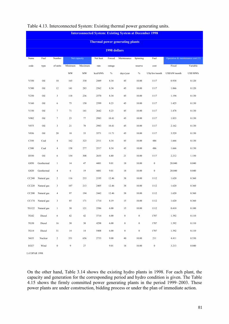
Table 4.13. Interconnected System: Existing thermal power generating units. Interconnected System: Existing System at December 1998

Thermal power generating plants

1998 dollars

Name Fuel Number Net capacity Net heat Forced Maintenance Spinning Fuel Operation & maintenance cost (1)

code type of units Minimum Maximum rate outage reserve cost Fixed Variable

MW MW kcal/kWh % days/year % US¢/kw/month US$/kW/month US$/MWh

V350 Oil 10 165 330 2449 8.34 45 10.00 1117 0.938 0.120

V300 Oil 12 141 283 2562 8.34 45 10.00 1117 1.066 0.120

V250 Oil 3 118 236 2570 8.34 45 10.00 1117 1.194 0.130

V160 Oil 6 75 150 2599 8.23 45 10.00 1117 1.425 0.130

V150 Oil 7 71 141 2642 8.23 45 10.00 1117 1.478 0.130

V082 Oil 7 23 77 2983 10.41 45 10.00 1117 1.833 0.130

V075 Oil 3 21 70 2983 10.41 45 10.00 1117 2.162 0.130

V036 Oil 20 10 33 3571 11.71 45 10.00 1117 3.529 0.130

C350 Coal 4 162 323 2511 8.34 45 10.00 486 1.666 0.130

C300 Coal 4 138 277 2517 8.34 45 10.00 486 1.666 0.130

D350 Oil 6 154 308 2655 6.80 21 10.00 1117 2.212 1.150

G050 Geothermal 1 14 47 4481 9.01 18 10.00 0 20.040 0.040

G020 Geothermal 4 6 19 4481 9.01 18 10.00 0 20.040 0.040

CC240 Natural gas 2 116 233 2195 12.46 38 10.00 1112 1.620 0.360

CC220 Natural gas 3 107 213 2405 12.46 38 10.00 1112 1.620 0.360

CC200 Natural gas 4 97 194 2442 12.46 38 10.00 1112 1.620 0.360

CC174 Natural gas 3 85 171 1714 8.19 15 10.00 1112 1.620 0.360

TG122 Natural gas 1 30 121 2586 6.00 15 10.00 1112 0.410 0.100

TG42 Diesel 6 42 42 3714 6.00 0 0 1787 1.392 0.110

TG30 Diesel 16 30 30 4298 6.00 0 0 1787 1.392 0.110

TG14 Diesel 31 14 14 5408 6.00 0 0 1787 1.392 0.110

N655 Nuclear 2 551 656 2733 9.00 40 10.00 211 4.411 0.530

EO27 Wind 0 9 27 9.01 18 10.00 0 3.213 0.040

1) COPAR 1998

On the other hand, Table 3.14 shows the existing hydro plants in 1998. For each plant, the capacity and generation for the corresponding period and hydro condition is given. The Table 4.15 shows the firmly committed power generating plants in the period 1999–2003. These power plants are under construction, bidding process or under the plan of immediate action.

81

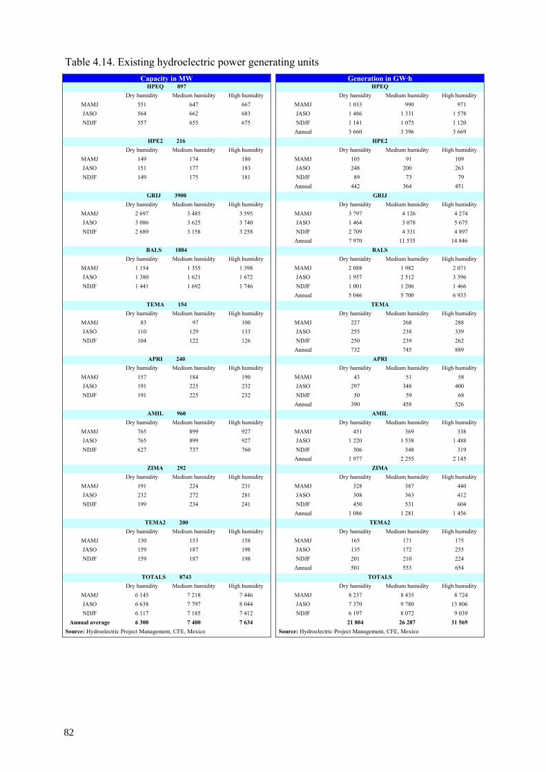
Table 4.14. Existing hydroelectric power generating units Capacity in MW Generation in GW·h

HPEQ 897 HPEQ Dry humidity Medium humidity High humidity Dry humidity Medium humidity High humidity

MAMJ 551 647 667 MAMJ 1 033 990 971 JASO 564 662 683 JASO 1 486 1 331 1 578 NDJF 557 655 675 NDJF 1 141 1 075 1 120

Annual 3 660 3 396 3 669 HPE2 216 HPE2

Dry humidity Medium humidity High humidity Dry humidity Medium humidity High humidity MAMJ 149 174 180 MAMJ 105 91 109 JASO 151 177 183 JASO 248 200 263 NDJF 149 175 181 NDJF 89 73 79

Annual 442 364 451 GRIJ 3900 GRIJ

Dry humidity Medium humidity High humidity Dry humidity Medium humidity High humidity MAMJ 2 697 3 485 3 595 MAMJ 3 797 4 126 4 274 JASO 3 086 3 625 3 740 JASO 1 464 3 078 5 675 NDJF 2 689 3 158 3 258 NDJF 2 709 4 331 4 897

Annual 7 970 11 535 14 846 BALS 1884 BALS


Annual 5 046 5 700 6 933 TEMA 154 TEMA


Annual 732 745 889 APRI 240 APRI


Annual 390 458 526 AMIL 960 AMIL

Dry humidity Medium humidity High humidity Dry humidity Medium humidity High humidity MAMJ 765 899 927 MAMJ 451 369 338 JASO 765 899 927 JASO 1 220 1 538 1 488 NDJF 627 737 760 NDJF 306 348 319

Annual 1 977 2 255 2 145 ZIMA 292 ZIMA


Annual 1 086 1 281 1 456 TEMA2 200 TEMA2


Annual 501 553 654 TOTALS 8743 TOTALS


Annual average 6 300 7 400 7 634 21 804 26 287 31 569 Source: Hydroelectric Project Management, CFE, Mexico Source: Hydroelectric Project Management, CFE, Mexico

82

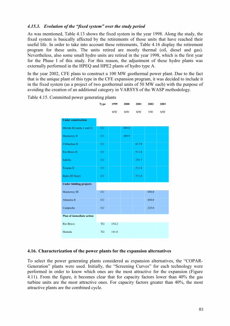
4.15.3. Evolution of the “fixed system” over the study period As was mentioned, Table 4.13 shows the fixed system in the year 1998. Along the study, the fixed system is basically affected by the retirements of those units that have reached their useful life. In order to take into account these retirements, Table 4.16 display the retirement program for these units. The units retired are mostly thermal (oil, diesel and gas). Nevertheless, also some small hydro units are retired in the year 1998, which is the first year for the Phase I of this study. For this reason, the adjustment of these hydro plants was externally performed in the HPEQ and HPE2 plants of hydro type A.

In the year 2002, CFE plans to construct a 100 MW geothermal power plant. Due to the fact that is the unique plant of this type in the CFE expansion program, it was decided to include it in the fixed system (as a project of two geothermal units of 50 MW each) with the purpose of avoiding the creation of an additional category in VARSYS of the WASP methodology.

Table 4.15. Committed power generating plants Type 1999 2000 2001 2002 2003

MW MW MW NW MW

Under construction

Mérida III (units 1 and 2) CC 499.0

Monterrey II CC 489.9

Chihuahua II CC 417.8

Río Bravo II CC 511.4

Saltillo CC 255.7

Tuxpan II CC 511.4

Bajío (El Sauz) CC 511.4

Under bidding projects

Monterrey III CC 450.0

Altamira II CC 450.0

Campeche CC 225.0

Plan of immediate action

Río Bravo TG 154.2

Huinala TG 141.0

4.16. Characterization of the power plants for the expansion alternatives

To select the power generating plants considered as expansion alternatives, the “COPAR-Generation” plants were used. Initially, the “Screening Curves” for each technology were performed in order to know which ones are the most attractive for the expansion (Figure 4.11). From the figure, it becomes clear that for capacity factors lower than 40% the gas turbine units are the most attractive ones. For capacity factors greater than 40%, the most attractive plants are the combined cycle.

83

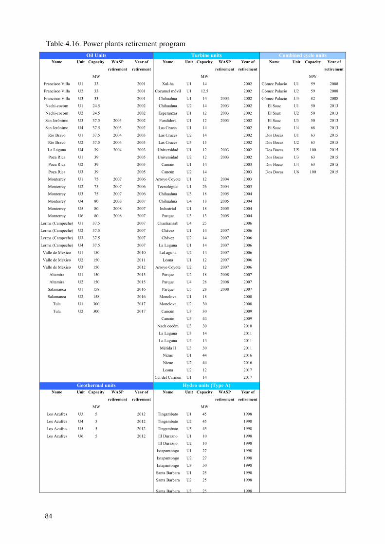
Table 4.16. Power plants retirement program Oil Units Turbine units Combined cycle units

Name Unit Capacity WASP Year of Name Unit Capacity WASP Year of Name Unit Capacity Year of

retirement retirement retirement retirement retirement

MW MW MW

Francisco Villa U1 33 2001 Xul-ha U1 14 2002 Gómez Palacio U1 59 2008

Francisco Villa U2 33 2001 Cozumel móvil U1 12.5 2002 Gómez Palacio U2 59 2008

Francisco Villa U3 33 2001 Chihuahua U1 14 2003 2002 Gómez Palacio U3 82 2008

Nachi-cocóm U1 24.5 2002 Chihuahua U2 14 2003 2002 El Sauz U1 50 2013

Nachi-cocóm U2 24.5 2002 Esperanzas U1 12 2003 2002 El Sauz U2 50 2013

San Jerónimo U3 37.5 2003 2002 Fundidora U1 12 2003 2002 El Sauz U3 50 2013

San Jerónimo U4 37.5 2003 2002 Las Cruces U1 14 2002 El Sauz U4 68 2013

Río Bravo U1 37.5 2004 2003 Las Cruces U2 14 2002 Dos Bocas U1 63 2015

Río Bravo U2 37.5 2004 2003 Las Cruces U3 15 2002 Dos Bocas U2 63 2015

La Laguna U4 39 2004 2003 Universidad U1 12 2003 2002 Dos Bocas U5 100 2015

Poza Rica U1 39 2005 Universidad U2 12 2003 2002 Dos Bocas U3 63 2015

Poza Rica U2 39 2005 Cancún U1 14 2003 Dos Bocas U4 63 2015

Poza Rica U3 39 2005 Cancún U2 14 2003 Dos Bocas U6 100 2015

Monterrey U1 75 2007 2006 Arroyo Coyote U1 12 2004 2003

Monterrey U2 75 2007 2006 Tecnológico U1 26 2004 2003

Monterrey U3 75 2007 2006 Chihuahua U3 18 2005 2004

Monterrey U4 80 2008 2007 Chihuahua U4 18 2005 2004

Monterrey U5 80 2008 2007 Industrial U1 18 2005 2004

Monterrey U6 80 2008 2007 Parque U3 13 2005 2004

Lerma (Campeche) U1 37.5 2007 Chankanaab U4 25 2006

Lerma (Campeche) U2 37.5 2007 Chávez U1 14 2007 2006

Lerma (Campeche) U3 37.5 2007 Chávez U2 14 2007 2006

Lerma (Campeche) U4 37.5 2007 La Laguna U1 14 2007 2006

Valle de México U1 150 2010 LaLaguna U2 14 2007 2006

Valle de México U2 150 2011 Leona U1 12 2007 2006

Valle de México U3 150 2012 Arroyo Coyote U2 12 2007 2006

Altamira U1 150 2015 Parque U2 18 2008 2007

Altamira U2 150 2015 Parque U4 28 2008 2007

Salamanca U1 158 2016 Parque U5 28 2008 2007

Salamanca U2 158 2016 Monclova U1 18 2008

Tula U1 300 2017 Monclova U2 30 2008

Tula U2 300 2017 Cancún U3 30 2009

Cancún U5 44 2009

Nach cocóm U3 30 2010

La Laguna U3 14 2011

La Laguna U4 14 2011

Mérida II U3 30 2011

Nizuc U1 44 2016

Nizuc U2 44 2016

Leona U2 12 2017

Cd. del Carmen U1 14 2017

Geothermal units Hydro units (Type A) Name Unit Capacity WASP Year of Name Unit Capacity WASP Year of

retirement retirement retirement retirement

MW MW

Los Azufres U3 5 2012 Tingambato U1 45 1998



Los Azufres U6 5 2012 El Durazno U1 10 1998

El Durazno U2 10 1998

Ixtapantongo U1 27 1998



Santa Barbara U1 25 1998



84

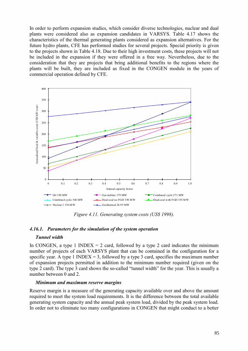
In order to perform expansion studies, which consider diverse technologies, nuclear and dual plants were considered also as expansion candidates in VARSYS. Table 4.17 shows the characteristics of the thermal generating plants considered as expansion alternatives. For the future hydro plants, CFE has performed studies for several projects. Special priority is given to the projects shown in Table 4.18. Due to their high investment costs, these projects will not be included in the expansion if they were offered in a free way. Nevertheless, due to the consideration that they are projects that bring additional benefits to the regions where the plants will be built, they are included as fixed in the CONGEN module in the years of commercial operation defined by CFE.

0 0.1 0.2 0.3 0.4 0.5 0.6 0.7 0.8 0.9 1.0

400

350

300

250

200

150

100

50

0


Oil 350 MW


Nuclear 1 356 MW

Gas turbine 179 MW

Dual-coal no FGD 350 MW

Geothermal 26.95 MW


Dual-coal with FGD 350 MW

Ann

ualiz

ed fi

xed

& v

aria

ble

cost

s ( U

S$/k

W-y

ear)

Figure 4.11. Generating system costs (US$ 1998).

4.16.1. Parameters for the simulation of the system operation

Tunnel width In CONGEN, a type 1 INDEX = 2 card, followed by a type 2 card indicates the minimum number of projects of each VARSYS plant that can be contained in the configuration for a specific year. A type 1 INDEX = 3, followed by a type 3 card, specifies the maximum number of expansion projects permitted in addition to the minimum number required (given on the type 2 card). The type 3 card shows the so-called “tunnel width” for the year. This is usually a number between 0 and 2.

Minimum and maximum reserve margins Reserve margin is a measure of the generating capacity available over and above the amount required to meet the system load requirements. It is the difference between the total available generating system capacity and the annual peak system load, divided by the peak system load. In order not to eliminate too many configurations in CONGEN that might conduct to a better

85

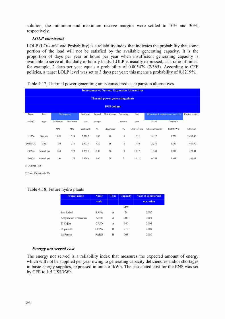
solution, the minimum and maximum reserve margins were settled to 10% and 30%, respectively.

LOLP constraint LOLP (LOss-of-Load Probability) is a reliability index that indicates the probability that some portion of the load will not be satisfied by the available generating capacity. It is the proportion of days per year or hours per year when insufficient generating capacity is available to serve all the daily or hourly loads. LOLP is usually expressed, as a ratio of times, for example, 2 days per year equals a probability of 0.005479 (2/365). According to CFE policies, a target LOLP level was set to 3 days per year; this means a probability of 0.8219%.

Table 4.17. Thermal power generating units considered as expansion alternatives Interconnected System: Expansion Alternatives

Thermal power generating plants

1998 dollars

Name Fuel Net capacity Net heat Forced Maintenance Spinning Fuel Operation & maintenance cost (1) Capital cost (1)

code (2) type Minimum Maximum rate outage reserve cost Fixed Variable

MW MW kcal/kWh % days/year % US¢/106 kcal US$/kW/month US$/MWh US$/kW

N1356 Nuclear 1 051 1 314 2 570.2 6.60 40 10 211 3.122 1.720 2 485.40

D350FGD Coal 155 310 2 597.4 7.10 36 10 486 2.280 1.180 1 467.90

CC546 Natural gas 264 527 1 762.8 10.00 26 10 1 112 1.348 0.310 427.44

TG179 Natural gas 44 175 2 624.4 6.00 26 0 1 112 0.355 0.078 346.03

1) COPAR 1998

2) Gross Capacity (MW)

Table 4.18. Future hydro plants Project name Name Type Capacity Year of commercial

code operation

MW

San Rafael RAFA A 24 2002

Ampliación Chicoasén ACHI A 900 2003

El Cajón CAJO A 640 2006

Copainalá COPA B 210 2008

La Parota PARO B 765 2008

Energy not served cost The energy not served is a reliability index that measures the expected amount of energy which will not be supplied per year owing to generating capacity deficiencies and/or shortages in basic energy supplies, expressed in units of kWh. The associated cost for the ENS was set by CFE to 1.5 US$/kWh.

86

Selection of the loading order

The loading order is calculated by MERSIM rearranging the basic economic L.O. of the thermal plants combined with FIXSYS and VARSYS. The MERSIM module will automatically dispatch base and peak blocks of the thermal plants in order to meet the spinning reserve (SPNRES) requirements of the system. SPNRES is given by the equation:

PKMWPEAKCAPSPNALSPNRES ×+×=

SPNAL = 1 (instruction b of card type 2 for our case)

CAP = largest unit capacity block already loaded

PEAKF = multiplier of PKMW = 1 (for our case)

PKMW = period peak load

4.16.2. Use of emission abatement technologies

Since the power plants in Mexico are in compliance with the environmental law NOM-085-ECOL-1994 is not necessary to add abatement technologies in the existing plants. On the other hand, the alternatives for expansion include abatement technologies, specifically:

• Dual plant includes one electrostatic precipitator and one wet FGD scrubber (Chiyoda-CT121) with efficiencies of 99.5% for particulates and 90% for SO2.

• The new combined cycle and the gas turbines have low NOX burners that guarantee NOX emissions lower than 110 ppm (0.281 kg NOX/106 kcal).

4.17. System-level analysis of generation system expansion

4.18. Base case analysis

4.18.1. Approach to reach the optimal solution

The process of generation planning for the Interconnected System shows that, in order to satisfy the growing electricity demand (5.5% growth rate), it is necessary to select the best technologies for the generation system expansion with a suitable level of reliability and minimum cost. Longer construction periods, cost and availability of fuels and expensive pollution control equipment must also be taken into consideration when a planner is deciding the number, type, and size of the generating units to be installed.

DECPAC module (WASP-III Plus version) of DECADES has been used to carry out the analysis of the base case and several different alternative plans for the future expansion of the power system over 27 years; the planning period is from 1998 to 2024. For the present study, Table 4.4 shows the thermal plant candidates that have been considered for future electric system expansion.

The combined cycle technology is very competitive because it uses a clean fuel (natural gas) and also has low investment costs, short construction periods and high thermal efficiency with respect to other technologies. As a result of these characteristics, it is the most attractive and competitive technology for the generation system expansion as it was already discussed and

87

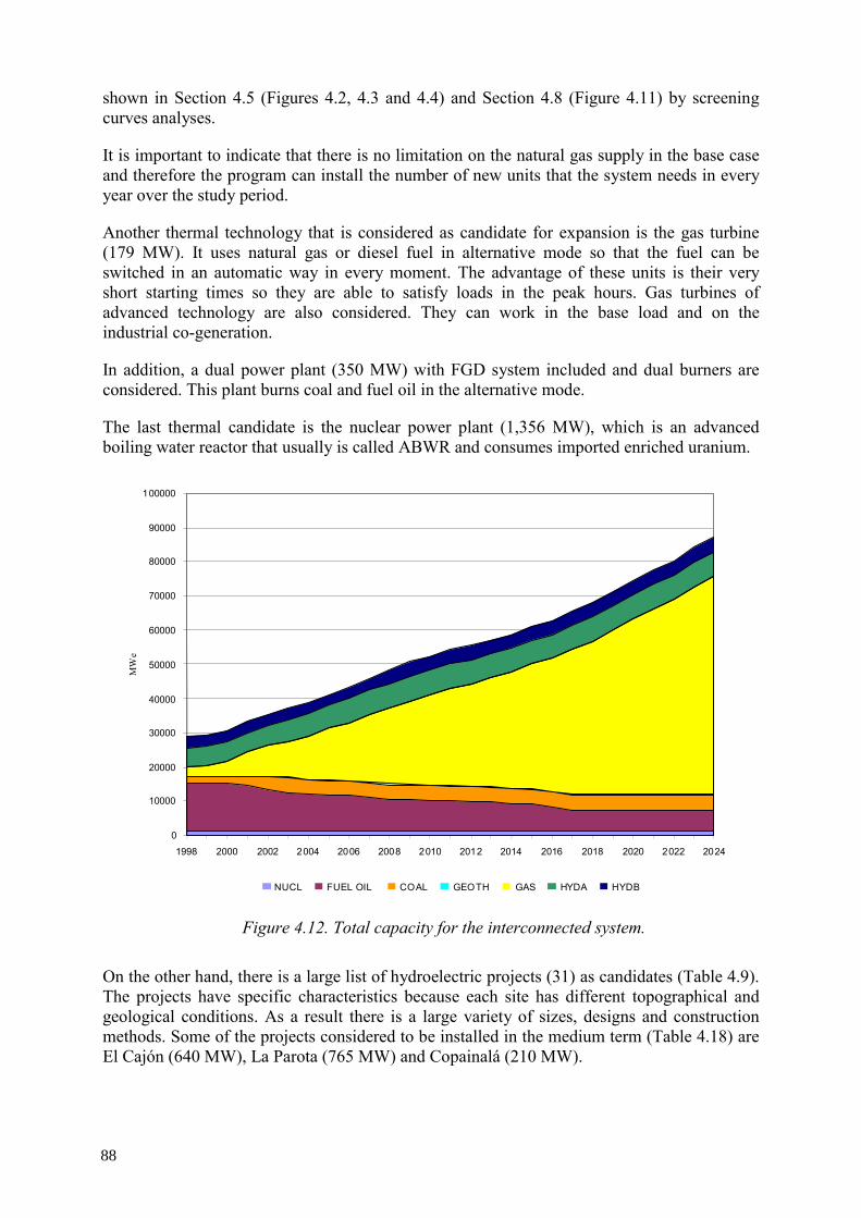
shown in Section 4.5 (Figures 4.2, 4.3 and 4.4) and Section 4.8 (Figure 4.11) by screening curves analyses.

It is important to indicate that there is no limitation on the natural gas supply in the base case and therefore the program can install the number of new units that the system needs in every year over the study period.

Another thermal technology that is considered as candidate for expansion is the gas turbine (179 MW). It uses natural gas or diesel fuel in alternative mode so that the fuel can be switched in an automatic way in every moment. The advantage of these units is their very short starting times so they are able to satisfy loads in the peak hours. Gas turbines of advanced technology are also considered. They can work in the base load and on the industrial co-generation.

In addition, a dual power plant (350 MW) with FGD system included and dual burners are considered. This plant burns coal and fuel oil in the alternative mode.

The last thermal candidate is the nuclear power plant (1,356 MW), which is an advanced boiling water reactor that usually is called ABWR and consumes imported enriched uranium.

0

10000

20000

30000

40000

50000

60000

70000

80000

90000

100000

1998 2000 2002 2004 2006 2008 2010 2012 2014 2016 2018 2020 2022 2024

NUCL FUEL OIL COAL GEOTH GAS HYDA HYDB

MW

e

Figure 4.12. Total capacity for the interconnected system.

On the other hand, there is a large list of hydroelectric projects (31) as candidates (Table 4.9). The projects have specific characteristics because each site has different topographical and geological conditions. As a result there is a large variety of sizes, designs and construction methods. Some of the projects considered to be installed in the medium term (Table 4.18) are El Cajón (640 MW), La Parota (765 MW) and Copainalá (210 MW).

88

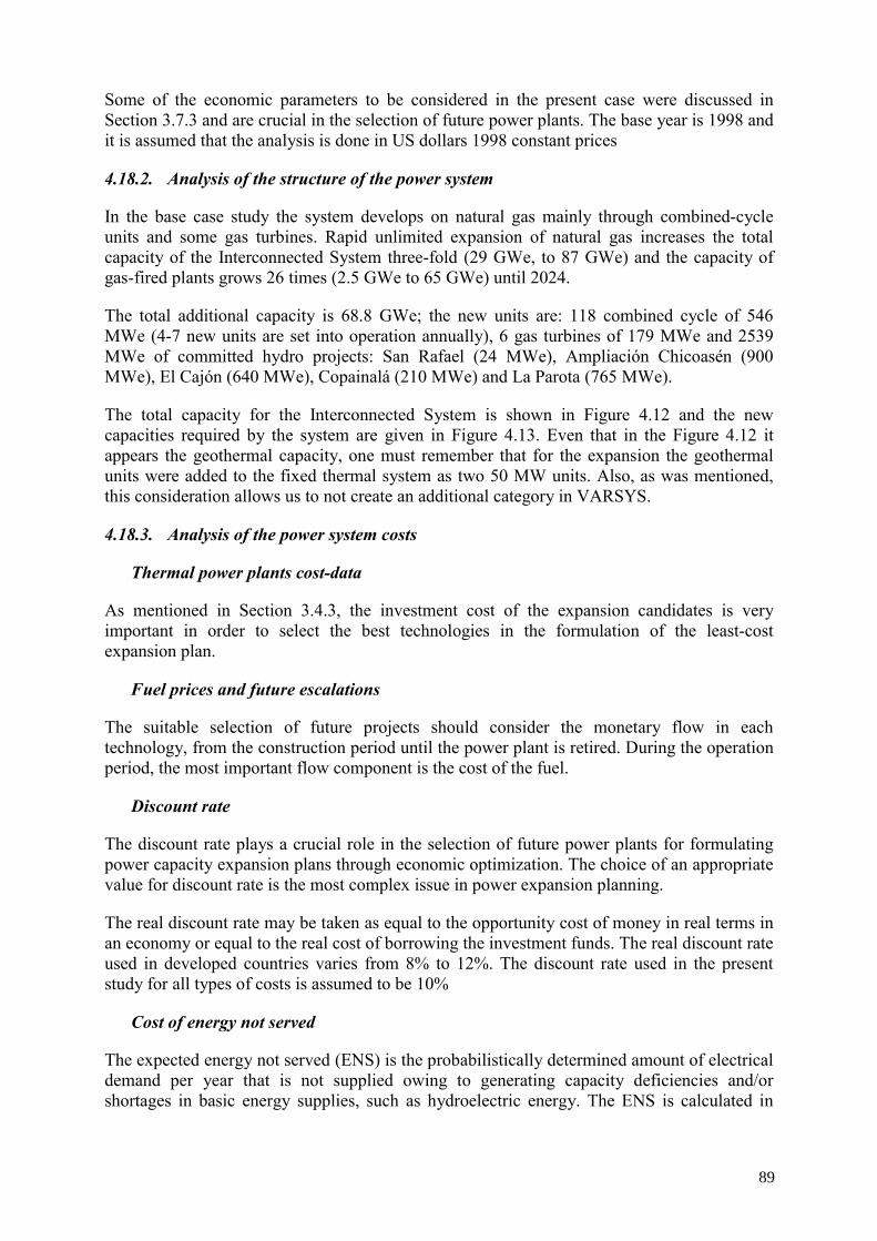
Some of the economic parameters to be considered in the present case were discussed in Section 3.7.3 and are crucial in the selection of future power plants. The base year is 1998 and it is assumed that the analysis is done in US dollars 1998 constant prices

4.18.2. Analysis of the structure of the power system

In the base case study the system develops on natural gas mainly through combined-cycle units and some gas turbines. Rapid unlimited expansion of natural gas increases the total capacity of the Interconnected System three-fold (29 GWe, to 87 GWe) and the capacity of gas-fired plants grows 26 times (2.5 GWe to 65 GWe) until 2024.

The total additional capacity is 68.8 GWe; the new units are: 118 combined cycle of 546 MWe (4-7 new units are set into operation annually), 6 gas turbines of 179 MWe and 2539 MWe of committed hydro projects: San Rafael (24 MWe), Ampliación Chicoasén (900 MWe), El Cajón (640 MWe), Copainalá (210 MWe) and La Parota (765 MWe).

The total capacity for the Interconnected System is shown in Figure 4.12 and the new capacities required by the system are given in Figure 4.13. Even that in the Figure 4.12 it appears the geothermal capacity, one must remember that for the expansion the geothermal units were added to the fixed thermal system as two 50 MW units. Also, as was mentioned, this consideration allows us to not create an additional category in VARSYS.

4.18.3. Analysis of the power system costs

Thermal power plants cost-data

As mentioned in Section 3.4.3, the investment cost of the expansion candidates is very important in order to select the best technologies in the formulation of the least-cost expansion plan.

Fuel prices and future escalations

The suitable selection of future projects should consider the monetary flow in each technology, from the construction period until the power plant is retired. During the operation period, the most important flow component is the cost of the fuel.

Discount rate

The discount rate plays a crucial role in the selection of future power plants for formulating power capacity expansion plans through economic optimization. The choice of an appropriate value for discount rate is the most complex issue in power expansion planning.

The real discount rate may be taken as equal to the opportunity cost of money in real terms in an economy or equal to the real cost of borrowing the investment funds. The real discount rate used in developed countries varies from 8% to 12%. The discount rate used in the present study for all types of costs is assumed to be 10%

Cost of energy not served

The expected energy not served (ENS) is the probabilistically determined amount of electrical demand per year that is not supplied owing to generating capacity deficiencies and/or shortages in basic energy supplies, such as hydroelectric energy. The ENS is calculated in

89

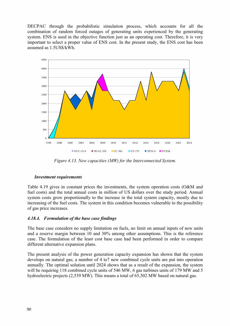
DECPAC through the probabilistic simulation process, which accounts for all the combination of random forced outages of generating units experienced by the generating system. ENS is used in the objective function just as an operating cost. Therefore, it is very important to select a proper value of ENS cost. In the present study, the ENS cost has been assumed as 1.5US$/kWh.

0

500

1000

1500

2000

2500

3000

3500

4000

4500

1998 2000 2002 2004 2006 2008 2010 2012 2014 2016 2018 2020 2022 2024

NUC-1314 DUAL-350 CC-546 GT-179 HYD-A HYD-B

Figure 4.13. New capacities (MW) for the Interconnected System.

Investment requirements

Table 4.19 gives in constant prices the investments, the system operation costs (O&M and fuel costs) and the total annual costs in million of US dollars over the study period. Annual system costs grow proportionally to the increase in the total system capacity, mostly due to increasing of the fuel costs. The system in this condition becomes vulnerable to the possibility of gas price increases.

4.18.4. Formulation of the base case findings

The base case considers no supply limitation on fuels, no limit on annual inputs of new units and a reserve margin between 10 and 30% among other assumptions. This is the reference case. The formulation of the least cost base case had been performed in order to compare different alternative expansion plans.

The present analysis of the power generation capacity expansion has shown that the system develops on natural gas; a number of 4 to7 new combined cycle units are put into operation annually. The optimal solution until 2024 shows that as a result of the expansion, the system will be requiring 118 combined cycle units of 546 MW, 6 gas turbines units of 179 MW and 5 hydroelectric projects (2,539 MW). This means a total of 65,502 MW based on natural gas.

90

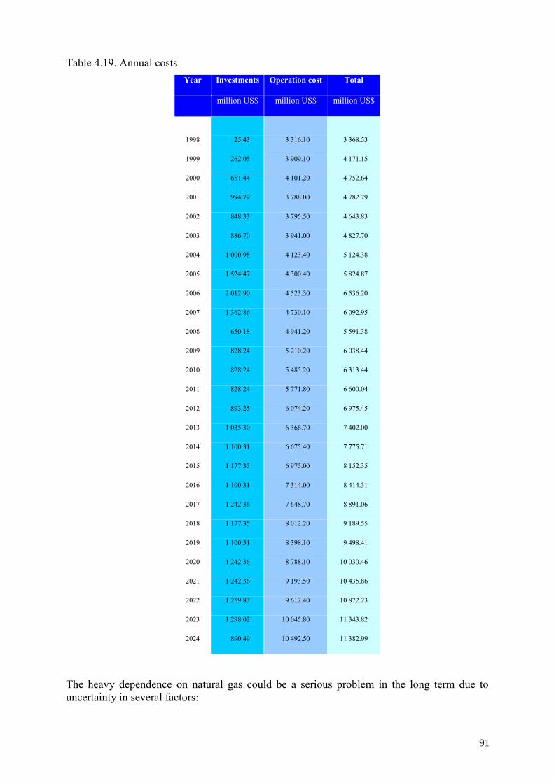
Table 4.19. Annual costs Year Investments Operation cost Total

million US$ million US$ million US$

1998 25.43 3 316.10 3 368.53

1999 262.05 3 909.10 4 171.15

2000 651.44 4 101.20 4 752.64

2001 994.79 3 788.00 4 782.79

2002 848.33 3 795.50 4 643.83

2003 886.70 3 941.00 4 827.70

2004 1 000.98 4 123.40 5 124.38

2005 1 524.47 4 300.40 5 824.87

2006 2 012.90 4 523.30 6 536.20

2007 1 362.86 4 730.10 6 092.95

2008 650.18 4 941.20 5 591.38

2009 828.24 5 210.20 6 038.44

2010 828.24 5 485.20 6 313.44

2011 828.24 5 771.80 6 600.04

2012 893.25 6 074.20 6 975.45

2013 1 035.30 6 366.70 7 402.00

2014 1 100.31 6 675.40 7 775.71

2015 1 177.35 6 975.00 8 152.35

2016 1 100.31 7 314.00 8 414.31

2017 1 242.36 7 648.70 8 891.06

2018 1 177.35 8 012.20 9 189.55

2019 1 100.31 8 398.10 9 498.41

2020 1 242.36 8 788.10 10 030.46

2021 1 242.36 9 193.50 10 435.86

2022 1 259.83 9 612.40 10 872.23

2023 1 298.02 10 045.80 11 343.82

2024 890.49 10 492.50 11 382.99

The heavy dependence on natural gas could be a serious problem in the long term due to uncertainty in several factors:

91

• In spite of the existing gas reserves in Mexico, there is an uncertainty on the domestic natural gas production in the long term, as well as on the infrastructure required to handle the gas;

• The growing national demand of natural gas in the different sectors;

• The demand growth is bigger than the supply and as a consequence there is a mayor dependence on gas imports, the uncertainly in gas imports is very high in the long term;

• The variability of international gas prices; and,

• The high demand of gas-fired technologies in the international market could be a limitation in the near future, because the new units will be imported.

It is important to mention that the 5 hydroelectric projects included in the expansion plan are committed plants. This means that no other hydro project is considered due to a very high investment costs.

On the other hand, the analysis of costs shows that the cumulative investments in present worth for capacity additions reached US$ 9,548 million and the cumulative system operation costs US$ 44,871 million (O&M and fuel costs) over the planning period. As a result, the total cost has been estimated in US$ 54,419 million.

In addition the annual system costs grow proportionally to the increase in the total system capacity, mostly due the increasing fuel costs. In these circumstances the system would be very vulnerable to the possibility of gas price increases.

During the operation of the power system it is assumed a reserve margin between 10 and 30%, the results showed that the system has a reserve around 33% in the first 10 years (medium term) and then it decreases up to 23% during the next 9 years and it reaches 18% in the last years of the period.

Another operation results are the reliability of the power system. In this case the LOLP in the medium term is very small, it is around 0.06 days/year; the LOLP reaches a value of 2.72 day/year during the last 6 years of the planning period, which is an acceptable value.

The analysis of the power system expansion has shown that the future electricity capacity is likely to be based on natural gas. Therefore, it is useful to perform an analysis with different alternative expansion plans in order to diversify the power system, considering all possible energy supply sources in the country and in this way obtain a robust expansion plan.

4.19. Scenario structure and analysis of expansion alternatives

4.19.1. Structure of the scenario alternatives

In order to study the impact of several possible causes on the expansion of the power sector it was considered convenient to develop a set of alternatives for the expansion of the sector. In addition to the Base Case, 13 alternatives were developed taking into account the following aspects or possibilities:

(1) Higher demand growth (6.5% demand growth rate instead 5% demand growth rate);

92

(2) Nuclear options (low nuclear cost and forced introduction);

(3) Escalation of fossil fuels (slightly higher fossil prices, notably higher gas prices and increase of the gas price in the medium term);

(4) Limitation in the introduction of new gas fired units (annual introduction of CC units is limited to 3 units/year and annual gas supply is limited starting 2010 (the gas limitation equals the gas supply in 2010);

(5) Variation of the discount rate (8% and 12% instead 10%); and,

(6) Changes in the target reliability (the reserve margins and/or the cost of energy not served (ENS) are defined to obtain a LOLP of 1 day per year, 5 days per year and a decreased reserve margin (by a decrease in the ENS value) for the early years of the period (this reflects the possible policy direction with respect to the reserve margin).

Table 3.20 shows the final list of expansion alternatives plans of the Interconnected System for this study. Besides, the description of the specific alternative it includes, for the Interconnected System, the set of expansion candidates for each alternative.

(a) Alternative A1: Impact of higher demand growth

Due to the uncertainty of the load growth, it was considered useful to analyze an alternative scenario for the demand; a higher demand growth rate of 6.5% instead of 5.5% considered in the Base Case.

(b) Analysis of the nuclear option

Two cases of sensitivity have been carried out for the nuclear option:

• Alternative B1: Considers low nuclear costs in which the investment cost of new nuclear power plant is assumed to be 48% lower than in the Base Case investment cost allowing new nuclear power plants to appear in the optimal solution.

• Alternative B2: Is a case of a forced nuclear introduction that includes one forced nuclear power plant of 1,356 MW in order to see the possible non-economic advantages of this additional nuclear power plant, for example lower emissions or a more diversified power system, and its impact on the system cost.

(c) Impact of the escalation of fossil fuel prices

With the purpose of analyze the effect on the escalation of fossil fuel prices in power expansion planning; three different cases have been performed:

• Alternative C1: Case of slightly higher fossil fuel prices. This case includes a slightly higher alternative projection for the escalation of fossil fuel prices (natural gas and the others).

• Alternative C2: Case of notably higher gas prices. Due to a recent increase of gas prices it has been assumed a higher projection for the prices of this fuel, 4 US$/tcf instead of 2.9 US$/tcf in the base case.

93

• Alternative C3: Case of a medium-term increase in the gas price. This case starts with a gas price of 2.9 US$/tcf as in the base case, next it considers a peak of 12 US$/tcf in 2010 and then a decline to 4 US$/tcf in 2024.

(d) Limitations on the introduction of new gas-fired units In order to evaluate the impact of reducing the number of new gas fired units due to technical reasons or gas supply constrains, two sensitivity analyses have been carried out:

• Alternative D1: Case of limitation on the number of CC-546 units; in this case the annual inputs of new combined cycle units of 546 MW are limited to 3 units per year instead of 4 to7 units as in the Base Case. The limitation starts in 2010.

• Alternative D2: Case of limited gas supply; natural gas imports are not firmly established after 2010, for this reason it is assumed that the annual gas supply is limited starting in 2010, the limit equals the gas supply in 2010.

(e) Variation of the discount rate Two cases with variation of the discount rate have been performed in order to see the impact on capital availability.

• Alternative E1: Case of increased discount rate; it is assumed a discount rate of 12% instead of 10% as in the Base Case, reflecting a higher cost of capital.

• Alternative E2: Case of decreased discount rate; it is assumed 8% instead 10% as in the Base Case, reflecting a lower cost of capital.

(f) Changes of the reliability

With the objective of analyzing different reliability criteria on the power system, three sensitivity analyses have been carried out.

• Alternative F1: Case of increased power system reliability; the cost of ENS is redefined to obtain a LOLP of one day per year (0.27%) instead of 3 days per year as in the Base Case.

• Alternative F2: Case of decreased power system reliability; in this case the cost of ENS is redefined to obtain a LOLP of 5 days per year (1.37%) instead of 3 days per year in the base case. The case will show the impact of the system becoming less reliable (e.g. as a result of deregulation)

• Alternative F3: Case of decreased reserve margin; the case is configured to obtain a lower reserve margin in the study by a decrease in the cost of ENS. This reflects the possible policy direction with respect to the reserve margin.

4.20. Analysis of the expansion alternatives

4.20.1. Impact of lower investment costs for new nuclear power plants

For Alternative B1 it has been assumed that the investment cost of a new nuclear power plant is 1,292 US$/kW instead of 2,485 US$/kW as in the Base Case. In this condition new nuclear power plants are competitive with the rest of the candidate technologies for expansion. In order to analyze the impact of new nuclear power plants on the power system the Alternative B1 has been considered.

94

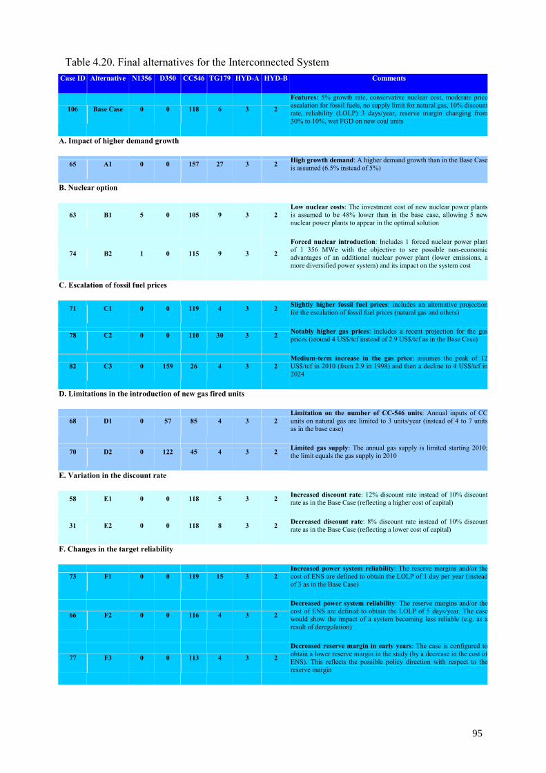
Table 4.20. Final alternatives for the Interconnected System Case ID Alternative N1356 D350 CC546 TG179 HYD-A HYD-B Comments

106 Base Case 0 0 118 6 3 2

Features: 5% growth rate, conservative nuclear cost, moderate price escalation for fossil fuels, no supply limit for natural gas, 10% discount rate, reliability (LOLP) 3 days/year, reserve margin changing from 30% to 10%, wet FGD on new coal units

A. Impact of higher demand growth

65 A1 0 0 157 27 3 2 High growth demand: A higher demand growth than in the Base Case is assumed (6.5% instead of 5%)

B. Nuclear option

63 B1 5 0 105 9 3 2 Low nuclear costs: The investment cost of new nuclear power plants is assumed to be 48% lower than in the base case, allowing 5 new nuclear power plants to appear in the optimal solution

74 B2 1 0 115 9 3 2

Forced nuclear introduction: Includes 1 forced nuclear power plant of 1 356 MWe with the objective to see possible non-economic advantages of an additional nuclear power plant (lower emissions, a more diversified power system) and its impact on the system cost

C. Escalation of fossil fuel prices

71 C1 0 0 119 4 3 2 Slightly higher fossil fuel prices: includes an alternative projection for the escalation of fossil fuel prices (natural gas and others)

78 C2 0 0 110 30 3 2 Notably higher gas prices: includes a recent projection for the gas prices (around 4 US$/tcf instead of 2.9 US$/tcf as in the Base Case)

82 C3 0 159 26 4 3 2 Medium-term increase in the gas price: assumes the peak of 12 US$/tcf in 2010 (from 2.9 in 1998) and then a decline to 4 US$/tcf in 2024

D. Limitations in the introduction of new gas fired units

68 D1 0 57 85 4 3 2 Limitation on the number of CC-546 units: Annual inputs of CC units on natural gas are limited to 3 units/year (instead of 4 to 7 units as in the base case)

70 D2 0 122 45 4 3 2 Limited gas supply: The annual gas supply is limited starting 2010; the limit equals the gas supply in 2010

E. Variation in the discount rate

58 E1 0 0 118 5 3 2 Increased discount rate: 12% discount rate instead of 10% discount rate as in the Base Case (reflecting a higher cost of capital)

31 E2 0 0 118 8 3 2 Decreased discount rate: 8% discount rate instead of 10% discount rate as in the Base Case (reflecting a lower cost of capital)

F. Changes in the target reliability

73 F1 0 0 119 15 3 2 Increased power system reliability: The reserve margins and/or the cost of ENS are defined to obtain the LOLP of 1 day per year (instead of 3 as in the Base Case)

66 F2 0 0 116 4 3 2

Decreased power system reliability: The reserve margins and/or the cost of ENS are defined to obtain the LOLP of 5 days/year. The case would show the impact of a system becoming less reliable (e.g. as a result of deregulation)

77 F3 0 0 113 4 3 2

Decreased reserve margin in early years: The case is configured to obtain a lower reserve margin in the study (by a decrease in the cost ofENS). This reflects the possible policy direction with respect to the reserve margin

95

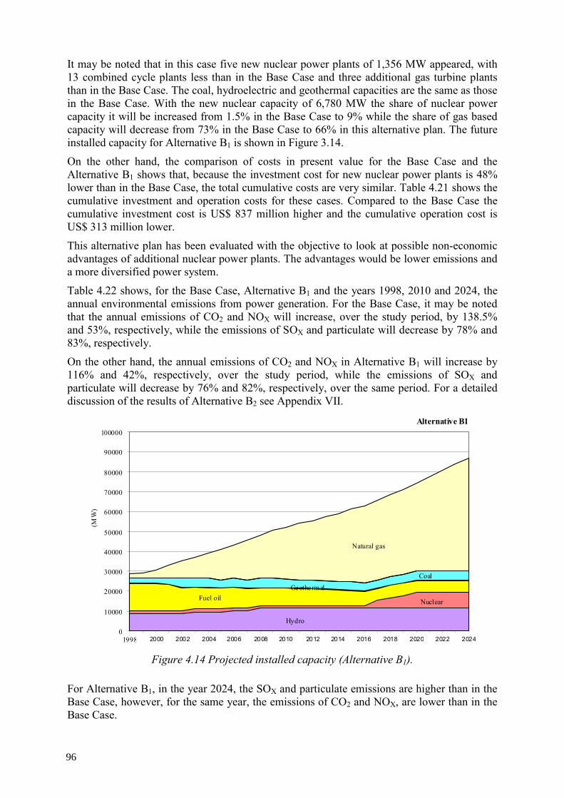
It may be noted that in this case five new nuclear power plants of 1,356 MW appeared, with 13 combined cycle plants less than in the Base Case and three additional gas turbine plants than in the Base Case. The coal, hydroelectric and geothermal capacities are the same as those in the Base Case. With the new nuclear capacity of 6,780 MW the share of nuclear power capacity it will be increased from 1.5% in the Base Case to 9% while the share of gas based capacity will decrease from 73% in the Base Case to 66% in this alternative plan. The future installed capacity for Alternative B1 is shown in Figure 3.14.

On the other hand, the comparison of costs in present value for the Base Case and the Alternative B1 shows that, because the investment cost for new nuclear power plants is 48% lower than in the Base Case, the total cumulative costs are very similar. Table 4.21 shows the cumulative investment and operation costs for these cases. Compared to the Base Case the cumulative investment cost is US$ 837 million higher and the cumulative operation cost is US$ 313 million lower.

This alternative plan has been evaluated with the objective to look at possible non-economic advantages of additional nuclear power plants. The advantages would be lower emissions and a more diversified power system.

Table 4.22 shows, for the Base Case, Alternative B1 and the years 1998, 2010 and 2024, the annual environmental emissions from power generation. For the Base Case, it may be noted that the annual emissions of CO2 and NOX will increase, over the study period, by 138.5% and 53%, respectively, while the emissions of SOX and particulate will decrease by 78% and 83%, respectively.

On the other hand, the annual emissions of CO2 and NOX in Alternative B1 will increase by 116% and 42%, respectively, over the study period, while the emissions of SOX and particulate will decrease by 76% and 82%, respectively, over the same period. For a detailed discussion of the results of Alternative B2 see Appendix VII.

Alternative B1

Hydro

Nuclear Fuel oil Geothermal

Coal

Natural gas

0

10000

20000

30000

40000

50000

60000

70000

80000

90000

100000

1998 2000 2002 2004 2006 2008 2010 2012 2014 2016 2018 2020 2022 2024

(MW

)

Figure 4.14 Projected installed capacity (Alternative B1).

For Alternative B1, in the year 2024, the SOX and particulate emissions are higher than in the Base Case, however, for the same year, the emissions of CO2 and NOX, are lower than in the Base Case.

96

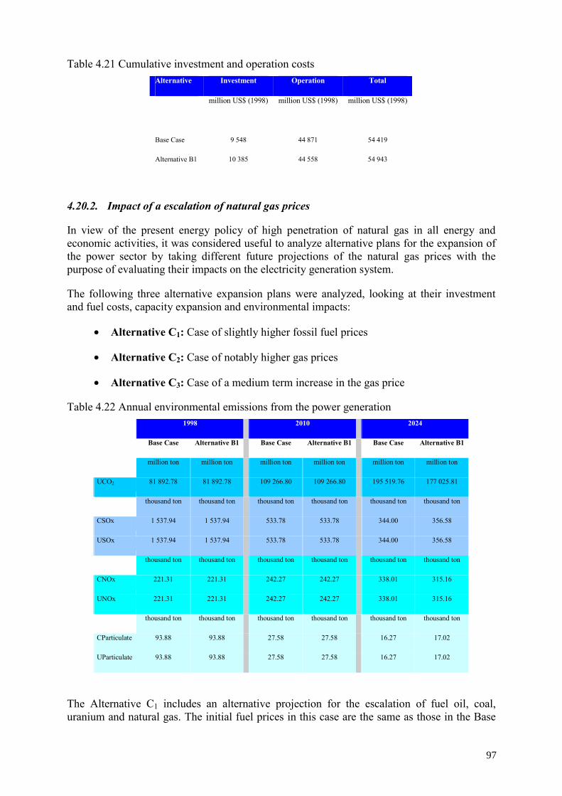
Table 4.21 Cumulative investment and operation costs Alternative Investment Operation Total

million US$ (1998) million US$ (1998) million US$ (1998)

Base Case 9 548 44 871 54 419

Alternative B1 10 385 44 558 54 943

4.20.2. Impact of a escalation of natural gas prices

In view of the present energy policy of high penetration of natural gas in all energy and economic activities, it was considered useful to analyze alternative plans for the expansion of the power sector by taking different future projections of the natural gas prices with the purpose of evaluating their impacts on the electricity generation system.

The following three alternative expansion plans were analyzed, looking at their investment and fuel costs, capacity expansion and environmental impacts:

• Alternative C1: Case of slightly higher fossil fuel prices

• Alternative C2: Case of notably higher gas prices

• Alternative C3: Case of a medium term increase in the gas price

Table 4.22 Annual environmental emissions from the power generation 1998 2010 2024

Base Case Alternative B1 Base Case Alternative B1 Base Case Alternative B1

million ton million ton million ton million ton million ton million ton

UCO2 81 892.78 81 892.78 109 266.80 109 266.80 195 519.76 177 025.81

thousand ton thousand ton thousand ton thousand ton thousand ton thousand ton

CSOx 1 537.94 1 537.94 533.78 533.78 344.00 356.58

USOx 1 537.94 1 537.94 533.78 533.78 344.00 356.58


CNOx 221.31 221.31 242.27 242.27 338.01 315.16

UNOx 221.31 221.31 242.27 242.27 338.01 315.16


CParticulate 93.88 93.88 27.58 27.58 16.27 17.02

UParticulate 93.88 93.88 27.58 27.58 16.27 17.02

The Alternative C1 includes an alternative projection for the escalation of fuel oil, coal, uranium and natural gas. The initial fuel prices in this case are the same as those in the Base

97

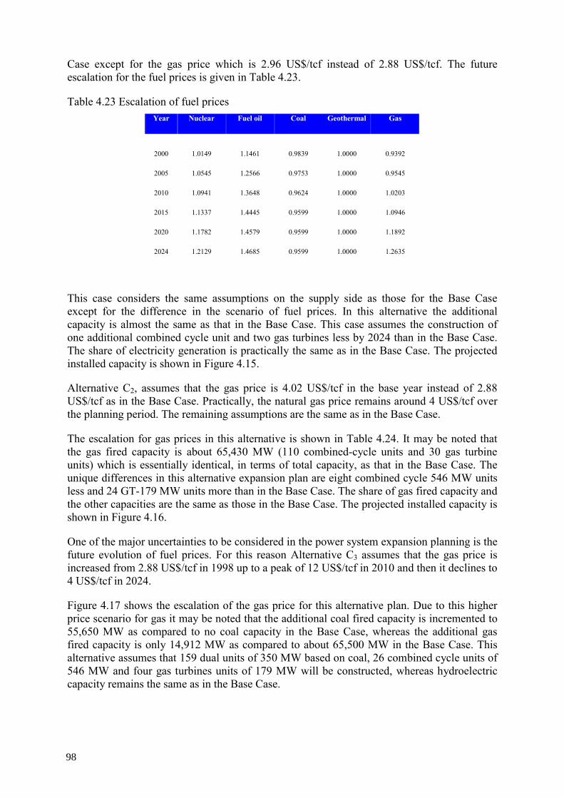
Case except for the gas price which is 2.96 US$/tcf instead of 2.88 US$/tcf. The future escalation for the fuel prices is given in Table 4.23.

Table 4.23 Escalation of fuel prices Year Nuclear Fuel oil Coal Geothermal Gas

2000 1.0149 1.1461 0.9839 1.0000 0.9392

2005 1.0545 1.2566 0.9753 1.0000 0.9545

2010 1.0941 1.3648 0.9624 1.0000 1.0203

2015 1.1337 1.4445 0.9599 1.0000 1.0946

2020 1.1782 1.4579 0.9599 1.0000 1.1892

2024 1.2129 1.4685 0.9599 1.0000 1.2635

This case considers the same assumptions on the supply side as those for the Base Case except for the difference in the scenario of fuel prices. In this alternative the additional capacity is almost the same as that in the Base Case. This case assumes the construction of one additional combined cycle unit and two gas turbines less by 2024 than in the Base Case. The share of electricity generation is practically the same as in the Base Case. The projected installed capacity is shown in Figure 4.15.

Alternative C2, assumes that the gas price is 4.02 US$/tcf in the base year instead of 2.88 US$/tcf as in the Base Case. Practically, the natural gas price remains around 4 US$/tcf over the planning period. The remaining assumptions are the same as in the Base Case.

The escalation for gas prices in this alternative is shown in Table 4.24. It may be noted that the gas fired capacity is about 65,430 MW (110 combined-cycle units and 30 gas turbine units) which is essentially identical, in terms of total capacity, as that in the Base Case. The unique differences in this alternative expansion plan are eight combined cycle 546 MW units less and 24 GT-179 MW units more than in the Base Case. The share of gas fired capacity and the other capacities are the same as those in the Base Case. The projected installed capacity is shown in Figure 4.16.

One of the major uncertainties to be considered in the power system expansion planning is the future evolution of fuel prices. For this reason Alternative C3 assumes that the gas price is increased from 2.88 US$/tcf in 1998 up to a peak of 12 US$/tcf in 2010 and then it declines to 4 US$/tcf in 2024.

Figure 4.17 shows the escalation of the gas price for this alternative plan. Due to this higher price scenario for gas it may be noted that the additional coal fired capacity is incremented to 55,650 MW as compared to no coal capacity in the Base Case, whereas the additional gas fired capacity is only 14,912 MW as compared to about 65,500 MW in the Base Case. This alternative assumes that 159 dual units of 350 MW based on coal, 26 combined cycle units of 546 MW and four gas turbines units of 179 MW will be constructed, whereas hydroelectric capacity remains the same as in the Base Case.

98

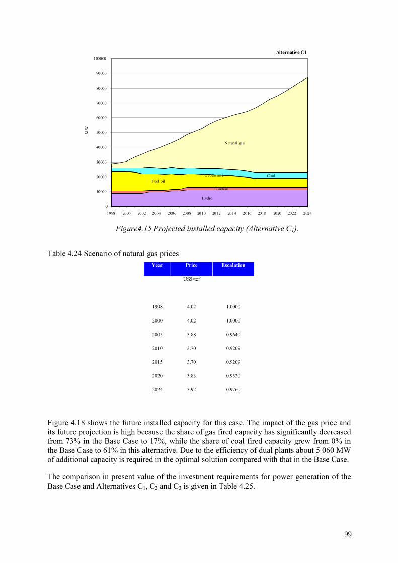
Alternative C1

Hydro

Nuclear

Fuel oilGeothermal Coal

Natural gas

0

10000

20000

30000

40000

50000

60000

70000

80000

90000

100000

1998 2000 2002 2004 2006 2008 2010 2012 2014 2016 2018 2020 2022 2024

MW

Figure4.15 Projected installed capacity (Alternative C1).

Table 4.24 Scenario of natural gas prices Year Price Escalation

US$/tcf

1998 4.02 1.0000

2000 4.02 1.0000

2005 3.88 0.9640

2010 3.70 0.9209

2015 3.70 0.9209

2020 3.83 0.9520

2024 3.92 0.9760

Figure 4.18 shows the future installed capacity for this case. The impact of the gas price and its future projection is high because the share of gas fired capacity has significantly decreased from 73% in the Base Case to 17%, while the share of coal fired capacity grew from 0% in the Base Case to 61% in this alternative. Due to the efficiency of dual plants about 5 060 MW of additional capacity is required in the optimal solution compared with that in the Base Case.

The comparison in present value of the investment requirements for power generation of the Base Case and Alternatives C1, C2 and C3 is given in Table 4.25.

99

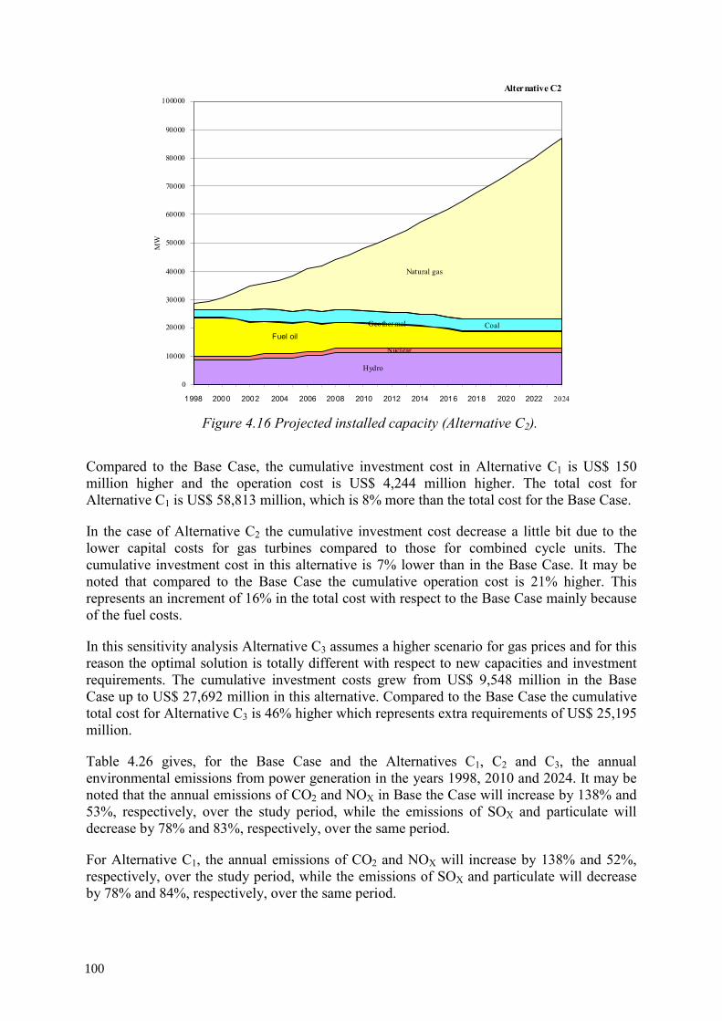
Alternative C2

Hydro

Nuclear

Fuel oil Geothermal Coal

Natural gas

0

10000

20000

30000

40000

50000

60000

70000

80000

90000

100000

1998 2000 2002 2004 2006 2008 2010 2012 2014 2016 2018 2020 2022 2024

MW

Figure 4.16 Projected installed capacity (Alternative C2).

Compared to the Base Case, the cumulative investment cost in Alternative C1 is US$ 150 million higher and the operation cost is US$ 4,244 million higher. The total cost for Alternative C1 is US$ 58,813 million, which is 8% more than the total cost for the Base Case.

In the case of Alternative C2 the cumulative investment cost decrease a little bit due to the lower capital costs for gas turbines compared to those for combined cycle units. The cumulative investment cost in this alternative is 7% lower than in the Base Case. It may be noted that compared to the Base Case the cumulative operation cost is 21% higher. This represents an increment of 16% in the total cost with respect to the Base Case mainly because of the fuel costs.

In this sensitivity analysis Alternative C3 assumes a higher scenario for gas prices and for this reason the optimal solution is totally different with respect to new capacities and investment requirements. The cumulative investment costs grew from US$ 9,548 million in the Base Case up to US$ 27,692 million in this alternative. Compared to the Base Case the cumulative total cost for Alternative C3 is 46% higher which represents extra requirements of US$ 25,195 million.

Table 4.26 gives, for the Base Case and the Alternatives C1, C2 and C3, the annual environmental emissions from power generation in the years 1998, 2010 and 2024. It may be noted that the annual emissions of CO2 and NOX in Base the Case will increase by 138% and 53%, respectively, over the study period, while the emissions of SOX and particulate will decrease by 78% and 83%, respectively, over the same period.

For Alternative C1, the annual emissions of CO2 and NOX will increase by 138% and 52%, respectively, over the study period, while the emissions of SOX and particulate will decrease by 78% and 84%, respectively, over the same period.

100

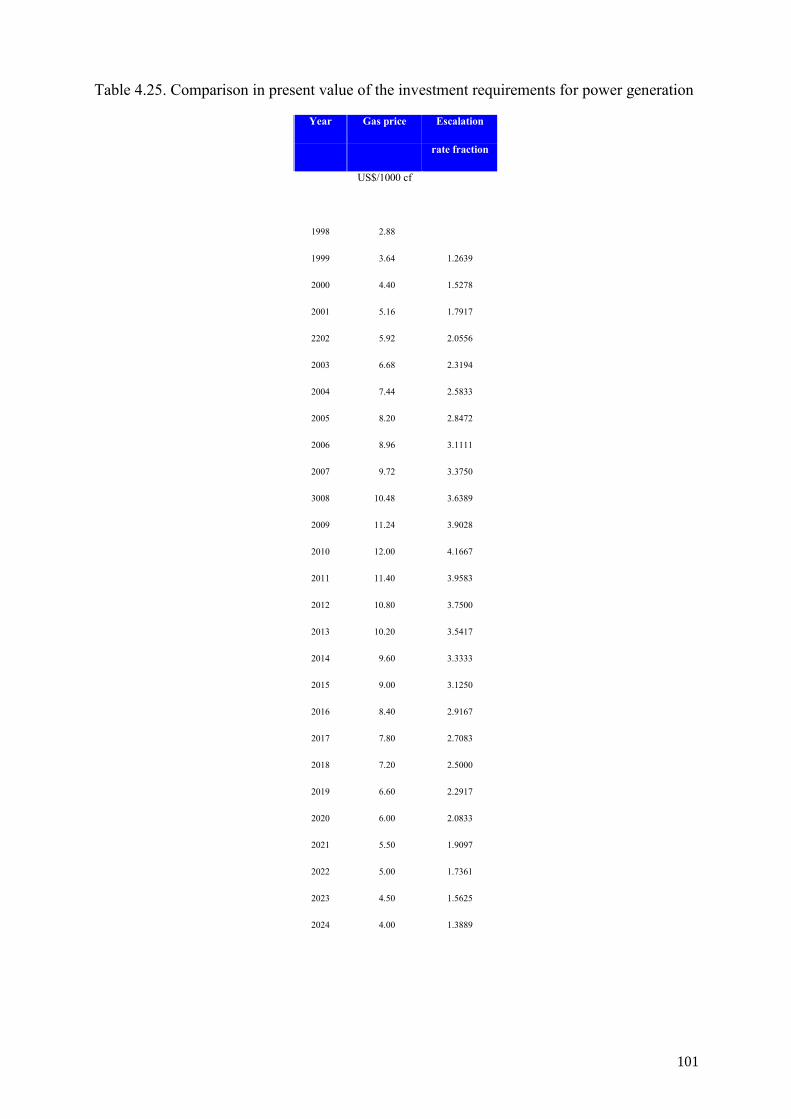
Table 4.25. Comparison in present value of the investment requirements for power generation

Year Gas price Escalation

rate fraction

US$/1000 cf

1998 2.88

1999 3.64 1.2639

2000 4.40 1.5278

2001 5.16 1.7917

2202 5.92 2.0556

2003 6.68 2.3194

2004 7.44 2.5833

2005 8.20 2.8472

2006 8.96 3.1111

2007 9.72 3.3750

3008 10.48 3.6389

2009 11.24 3.9028

2010 12.00 4.1667

2011 11.40 3.9583

2012 10.80 3.7500

2013 10.20 3.5417

2014 9.60 3.3333

2015 9.00 3.1250

2016 8.40 2.9167

2017 7.80 2.7083

2018 7.20 2.5000

2019 6.60 2.2917

2020 6.00 2.0833

2021 5.50 1.9097

2022 5.00 1.7361

2023 4.50 1.5625

2024 4.00 1.3889

101

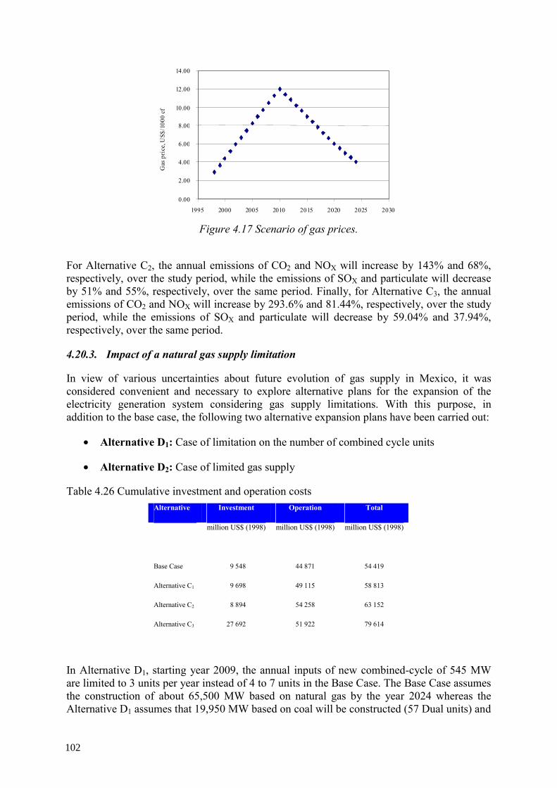
Gas

pri

ce, U

S$/1

000

cf

0.00

2.00

4.00

6.00

8.00

10.00

12.00

14.00

1995 2000 2005 2010 2015 2020 2025 2030

Figure 4.17 Scenario of gas prices.

For Alternative C2, the annual emissions of CO2 and NOX will increase by 143% and 68%, respectively, over the study period, while the emissions of SOX and particulate will decrease by 51% and 55%, respectively, over the same period. Finally, for Alternative C3, the annual emissions of CO2 and NOX will increase by 293.6% and 81.44%, respectively, over the study period, while the emissions of SOX and particulate will decrease by 59.04% and 37.94%, respectively, over the same period.

4.20.3. Impact of a natural gas supply limitation

In view of various uncertainties about future evolution of gas supply in Mexico, it was considered convenient and necessary to explore alternative plans for the expansion of the electricity generation system considering gas supply limitations. With this purpose, in addition to the base case, the following two alternative expansion plans have been carried out:

• Alternative D1: Case of limitation on the number of combined cycle units

• Alternative D2: Case of limited gas supply



Base Case 9 548 44 871 54 419

Alternative C1 9 698 49 115 58 813

Alternative C2 8 894 54 258 63 152

Alternative C3 27 692 51 922 79 614

In Alternative D1, starting year 2009, the annual inputs of new combined-cycle of 545 MW are limited to 3 units per year instead of 4 to 7 units in the Base Case. The Base Case assumes the construction of about 65,500 MW based on natural gas by the year 2024 whereas the Alternative D1 assumes that 19,950 MW based on coal will be constructed (57 Dual units) and

102

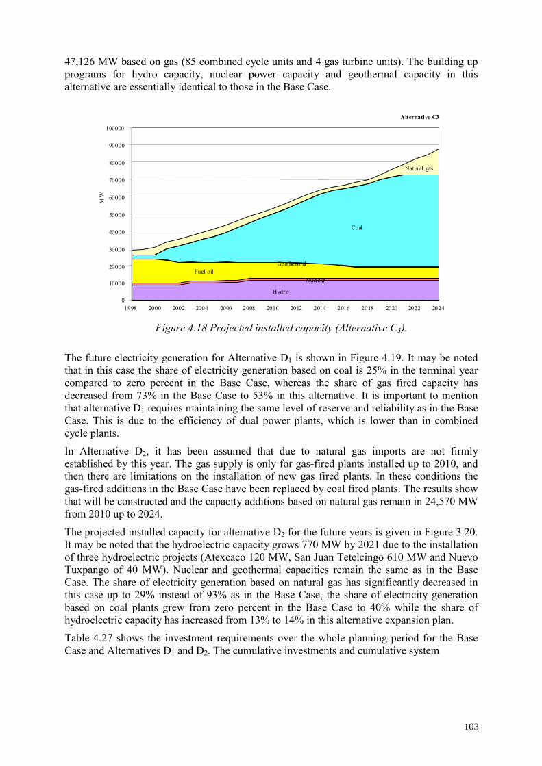
47,126 MW based on gas (85 combined cycle units and 4 gas turbine units). The building up programs for hydro capacity, nuclear power capacity and geothermal capacity in this alternative are essentially identical to those in the Base Case.

Alternative C3

Hydro

NuclearFuel oil

Geothe rmal

Coal

Natural gas

0 10000

20000

30000

40000

50000

60000

70000

80000

90000

100000

1998 2000 2002 2004 2006 2008 2010 2012 2014 2016 2018 2020 2022 2024

MW

Figure 4.18 Projected installed capacity (Alternative C3).

The future electricity generation for Alternative D1 is shown in Figure 4.19. It may be noted that in this case the share of electricity generation based on coal is 25% in the terminal year compared to zero percent in the Base Case, whereas the share of gas fired capacity has decreased from 73% in the Base Case to 53% in this alternative. It is important to mention that alternative D1 requires maintaining the same level of reserve and reliability as in the Base Case. This is due to the efficiency of dual power plants, which is lower than in combined cycle plants.

In Alternative D2, it has been assumed that due to natural gas imports are not firmly established by this year. The gas supply is only for gas-fired plants installed up to 2010, and then there are limitations on the installation of new gas fired plants. In these conditions the gas-fired additions in the Base Case have been replaced by coal fired plants. The results show that will be constructed and the capacity additions based on natural gas remain in 24,570 MW from 2010 up to 2024.

The projected installed capacity for alternative D2 for the future years is given in Figure 3.20. It may be noted that the hydroelectric capacity grows 770 MW by 2021 due to the installation of three hydroelectric projects (Atexcaco 120 MW, San Juan Tetelcingo 610 MW and Nuevo Tuxpango of 40 MW). Nuclear and geothermal capacities remain the same as in the Base Case. The share of electricity generation based on natural gas has significantly decreased in this case up to 29% instead of 93% as in the Base Case, the share of electricity generation based on coal plants grew from zero percent in the Base Case to 40% while the share of hydroelectric capacity has increased from 13% to 14% in this alternative expansion plan.

Table 4.27 shows the investment requirements over the whole planning period for the Base Case and Alternatives D1 and D2. The cumulative investments and cumulative system

103

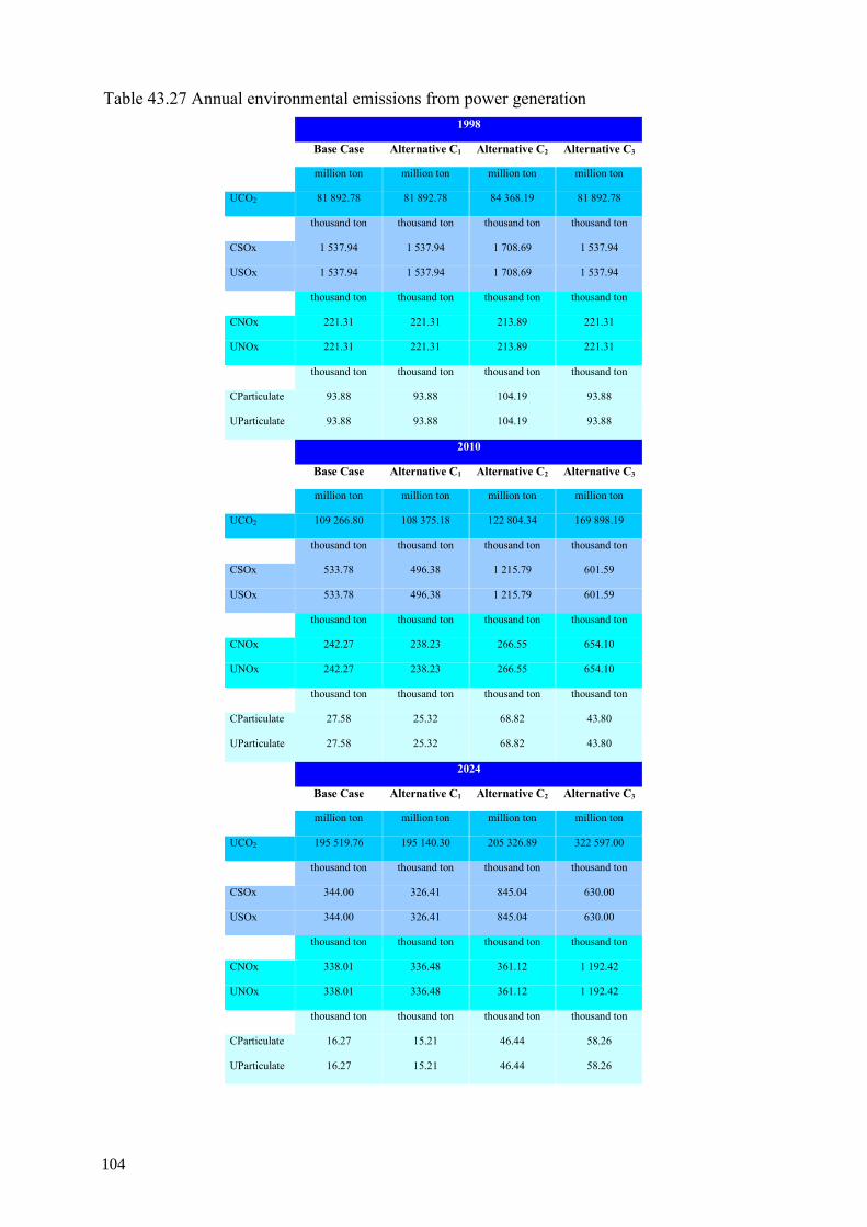
Table 43.27 Annual environmental emissions from power generation 1998

Base Case Alternative C1 Alternative C2 Alternative C3

million ton million ton million ton million ton

UCO2 81 892.78 81 892.78 84 368.19 81 892.78

thousand ton thousand ton thousand ton thousand ton

CSOx 1 537.94 1 537.94 1 708.69 1 537.94

USOx 1 537.94 1 537.94 1 708.69 1 537.94


CNOx 221.31 221.31 213.89 221.31

UNOx 221.31 221.31 213.89 221.31


CParticulate 93.88 93.88 104.19 93.88

UParticulate 93.88 93.88 104.19 93.88

2010



UCO2 109 266.80 108 375.18 122 804.34 169 898.19


CSOx 533.78 496.38 1 215.79 601.59

USOx 533.78 496.38 1 215.79 601.59


CNOx 242.27 238.23 266.55 654.10

UNOx 242.27 238.23 266.55 654.10


CParticulate 27.58 25.32 68.82 43.80

UParticulate 27.58 25.32 68.82 43.80

2024



UCO2 195 519.76 195 140.30 205 326.89 322 597.00


CSOx 344.00 326.41 845.04 630.00

USOx 344.00 326.41 845.04 630.00


CNOx 338.01 336.48 361.12 1 192.42

UNOx 338.01 336.48 361.12 1 192.42


CParticulate 16.27 15.21 46.44 58.26

UParticulate 16.27 15.21 46.44 58.26

104

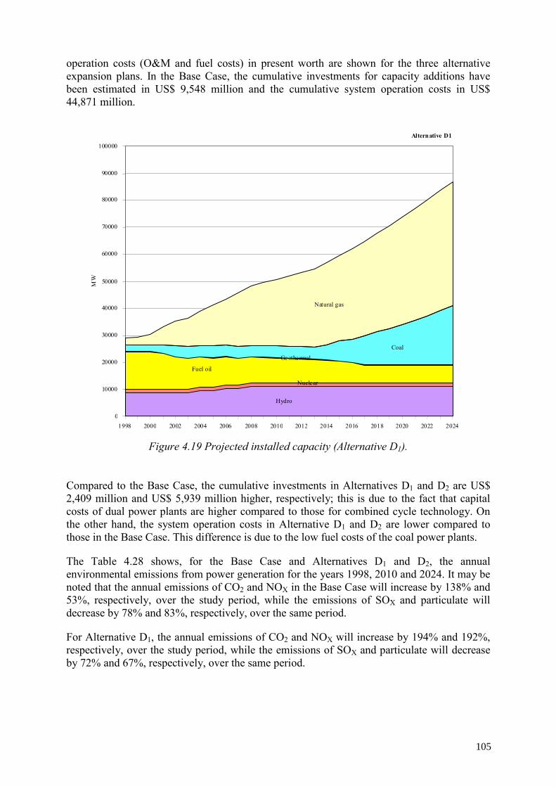
operation costs (O&M and fuel costs) in present worth are shown for the three alternative expansion plans. In the Base Case, the cumulative investments for capacity additions have been estimated in US$ 9,548 million and the cumulative system operation costs in US$ 44,871 million.

Alternative D1

Hydro

Nuclear

Fuel oil

Geothermal

Coal

Natural gas

0

10000

20000

30000

40000

50000

60000

70000

80000

90000

100000

1998 2000 2002 2004 2006 2008 2010 2012 2014 2016 2018 2020 2022 2024

MW

Figure 4.19 Projected installed capacity (Alternative D1).

Compared to the Base Case, the cumulative investments in Alternatives D1 and D2 are US$ 2,409 million and US$ 5,939 million higher, respectively; this is due to the fact that capital costs of dual power plants are higher compared to those for combined cycle technology. On the other hand, the system operation costs in Alternative D1 and D2 are lower compared to those in the Base Case. This difference is due to the low fuel costs of the coal power plants.

The Table 4.28 shows, for the Base Case and Alternatives D1 and D2, the annual environmental emissions from power generation for the years 1998, 2010 and 2024. It may be noted that the annual emissions of CO2 and NOX in the Base Case will increase by 138% and 53%, respectively, over the study period, while the emissions of SOX and particulate will decrease by 78% and 83%, respectively, over the same period.

For Alternative D1, the annual emissions of CO2 and NOX will increase by 194% and 192%, respectively, over the study period, while the emissions of SOX and particulate will decrease by 72% and 67%, respectively, over the same period.

105

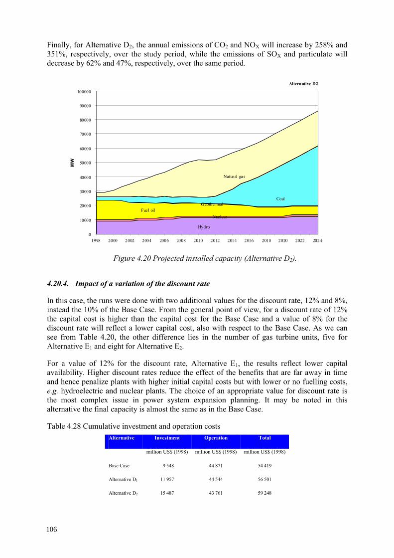
Finally, for Alternative D2, the annual emissions of CO2 and NOX will increase by 258% and 351%, respectively, over the study period, while the emissions of SOX and particulate will decrease by 62% and 47%, respectively, over the same period.

Alternative D2

Hydro

NuclearFuel oil

GeothermalCoal

Natural gas

0

10000

20000

30000

40000

50000

60000

70000

80000

90000

100000

1998 2000 2002 2004 2006 2008 2010 2012 2014 2016 2018 2020 2022 2024

MW

Figure 4.20 Projected installed capacity (Alternative D2).

4.20.4. Impact of a variation of the discount rate

In this case, the runs were done with two additional values for the discount rate, 12% and 8%, instead the 10% of the Base Case. From the general point of view, for a discount rate of 12% the capital cost is higher than the capital cost for the Base Case and a value of 8% for the discount rate will reflect a lower capital cost, also with respect to the Base Case. As we can see from Table 4.20, the other difference lies in the number of gas turbine units, five for Alternative E1 and eight for Alternative E2.

For a value of 12% for the discount rate, Alternative E1, the results reflect lower capital availability. Higher discount rates reduce the effect of the benefits that are far away in time and hence penalize plants with higher initial capital costs but with lower or no fuelling costs, e.g. hydroelectric and nuclear plants. The choice of an appropriate value for discount rate is the most complex issue in power system expansion planning. It may be noted in this alternative the final capacity is almost the same as in the Base Case.



Base Case 9 548 44 871 54 419

Alternative D1 11 957 44 544 56 501

Alternative D2 15 487 43 761 59 248

106

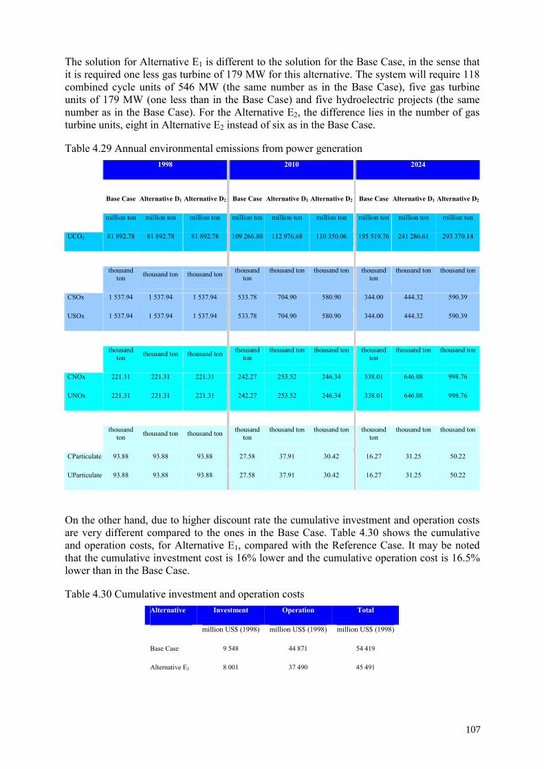
The solution for Alternative E1 is different to the solution for the Base Case, in the sense that it is required one less gas turbine of 179 MW for this alternative. The system will require 118 combined cycle units of 546 MW (the same number as in the Base Case), five gas turbine units of 179 MW (one less than in the Base Case) and five hydroelectric projects (the same number as in the Base Case). For the Alternative E2, the difference lies in the number of gas turbine units, eight in Alternative E2 instead of six as in the Base Case.

Table 4.29 Annual environmental emissions from power generation 1998 2010 2024

Base Case Alternative D1 Alternative D2 Base Case Alternative D1 Alternative D2 Base Case Alternative D1 Alternative D2

million ton million ton million ton million ton million ton million ton million ton million ton million ton

UCO2 81 892.78 81 892.78 81 892.78 109 266.80 112 976.68 110 350.06 195 519.76 241 286.61 293 370.14

thousand ton thousand ton thousand ton thousand

ton thousand ton thousand ton thousand

ton thousand ton thousand ton

CSOx 1 537.94 1 537.94 1 537.94 533.78 704.90 580.90 344.00 444.32 590.39

USOx 1 537.94 1 537.94 1 537.94 533.78 704.90 580.90 344.00 444.32 590.39




CNOx 221.31 221.31 221.31 242.27 253.52 246.34 338.01 646.08 998.76

UNOx 221.31 221.31 221.31 242.27 253.52 246.34 338.01 646.08 998.76




CParticulate 93.88 93.88 93.88 27.58 37.91 30.42 16.27 31.25 50.22

UParticulate 93.88 93.88 93.88 27.58 37.91 30.42 16.27 31.25 50.22

On the other hand, due to higher discount rate the cumulative investment and operation costs are very different compared to the ones in the Base Case. Table 4.30 shows the cumulative and operation costs, for Alternative E1, compared with the Reference Case. It may be noted that the cumulative investment cost is 16% lower and the cumulative operation cost is 16.5% lower than in the Base Case.



Base Case 9 548 44 871 54 419

Alternative E1 8 001 37 490 45 491

107

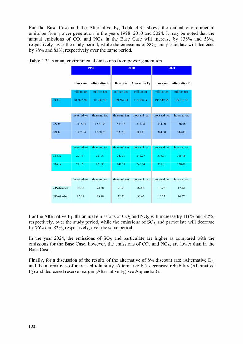
For the Base Case and the Alternative E1, Table 4.31 shows the annual environmental emission from power generation in the years 1998, 2010 and 2024. It may be noted that the annual emissions of CO2 and NOX in the Base Case will increase by 138% and 53%, respectively, over the study period, while the emissions of SOX and particulate will decrease by 78% and 83%, respectively over the same period.

Table 4.31 Annual environmental emissions from power generation 1998 2010 2024

Base case Alternative E1 Base case Alternative E1 base case Alternative E1

million ton million ton million ton million ton million ton million ton

UCO2 81 982.78 81 982.78 109 266.80 110 350.06 195 519.76 195 516.70


CSOx 1 537.94 1 537.94 533.78 533.78 344.00 356.58

USOx 1 537.94 1 538.50 533.78 581.01 344.00 344.03


CNOx 221.31 221.31 242.27 242.27 338.01 315.16

UNOx 221.31 221.31 242.27 246.34 338.01 338.02


CParticulate 93.88 93.88 27.58 27.58 16.27 17.02

UParticulate 93.88 93.88 27.58 30.42 16.27 16.27

For the Alternative E1, the annual emissions of CO2 and NOX will increase by 116% and 42%, respectively, over the study period, while the emissions of SOX and particulate will decrease by 76% and 82%, respectively, over the same period.

In the year 2024, the emissions of SOX and particulate are higher as compared with the emissions for the Base Case, however, the emissions of CO2 and NOX, are lower than in the Base Case.

Finally, for a discussion of the results of the alternative of 8% discount rate (Alternative E2) and the alternatives of increased reliability (Alternative F1), decreased reliability (Alternative F2) and decreased reserve margin (Alternative F3) see Appendix G.

108

5. TOTAL ENERGY SYSTEM ANALYSIS

For the second phase of the project entitled: "Comparative Assessment of Energy Options and Strategies until 2025”, the total energy system in Mexico was analyzed by using ENPEP model. This chapter and following chapter concentrate on this study. This chapter focuses on the scope of the ENPEP study, giving the various scenarios and their assumptions as well as the configuration of the total energy network in Mexico.

5.1. Scope of total energy system analysis

The specific objectives of the study were:

• To identify domestic supply sufficiency for major energy resources, the long term need for energy imports, and the potential for energy exports;

• To study energy infrastructure development to support the growing energy use in Mexico;

• To analyze, in view of the projected high reliance of the power system and other demand sectors on natural gas, the development of the gas sector in detail in order to identify possible supply constraints, price implications and relevant policy measures:

• To identify the potential role of renewable energy sources in the Mexican energy system;

• To quantify environmental emissions of the whole energy sector associated with the expected growth of energy consumption and possible emission mitigation measures;

• To provide, by considering several alternative scenarios, a set of possible scenarios as input to national decision-making in the energy sector.

Therefore the modeling scope includes the energy supply sectors (oil, gas, coal, nuclear and renewable energy sources), energy conversion sectors (coal processing, oil refining, gas processing, power generation, etc.), energy transportation and distribution (distribution of oil, gas, and refinery products, coal distribution, electricity transmission and distribution, etc.), energy use at the demand side (modeled at the level of final or useful energy as appropriate) and emissions.

The studies comprise four case analyses based on the different scenarios — baseline scenario and three alternative scenarios. The entire energy system network is configured in a way that the various alternative scenarios analyses could be carried out.

The reference case — baseline scenario — corresponds to the unlimited supply of natural gas, either domestic or imported natural gas or both. The main assumptions for this scenario are:

• Utilize domestic resources to the extent possible

• Maintain energy diversity and avoid dependency on a single source

• Increase the use of natural gas, considering unlimited supply of natural gas; not just in the availability of this energy source but also for availability of the infrastructure for the transportation and distribution of the energy source;

• Consider utilization of advanced environmentally friendly technologies in the energy supply system;

109

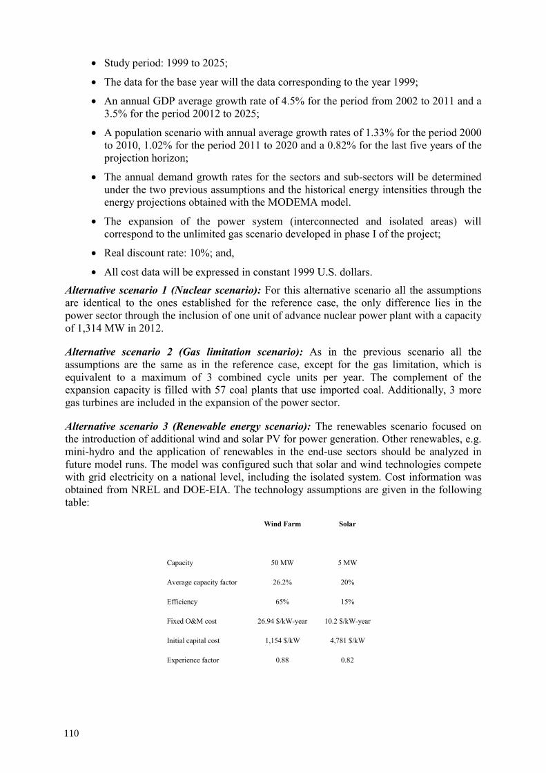
• Study period: 1999 to 2025;

• The data for the base year will the data corresponding to the year 1999;

• An annual GDP average growth rate of 4.5% for the period from 2002 to 2011 and a 3.5% for the period 20012 to 2025;

• A population scenario with annual average growth rates of 1.33% for the period 2000 to 2010, 1.02% for the period 2011 to 2020 and a 0.82% for the last five years of the projection horizon;

• The annual demand growth rates for the sectors and sub-sectors will be determined under the two previous assumptions and the historical energy intensities through the energy projections obtained with the MODEMA model.

• The expansion of the power system (interconnected and isolated areas) will correspond to the unlimited gas scenario developed in phase I of the project;

• Real discount rate: 10%; and,

• All cost data will be expressed in constant 1999 U.S. dollars. Alternative scenario 1 (Nuclear scenario): For this alternative scenario all the assumptions are identical to the ones established for the reference case, the only difference lies in the power sector through the inclusion of one unit of advance nuclear power plant with a capacity of 1,314 MW in 2012.

Alternative scenario 2 (Gas limitation scenario): As in the previous scenario all the assumptions are the same as in the reference case, except for the gas limitation, which is equivalent to a maximum of 3 combined cycle units per year. The complement of the expansion capacity is filled with 57 coal plants that use imported coal. Additionally, 3 more gas turbines are included in the expansion of the power sector.

Alternative scenario 3 (Renewable energy scenario): The renewables scenario focused on the introduction of additional wind and solar PV for power generation. Other renewables, e.g. mini-hydro and the application of renewables in the end-use sectors should be analyzed in future model runs. The model was configured such that solar and wind technologies compete with grid electricity on a national level, including the isolated system. Cost information was obtained from NREL and DOE-EIA. The technology assumptions are given in the following table:

Wind Farm Solar

Capacity 50 MW 5 MW

Average capacity factor 26.2% 20%

Efficiency 65% 15%

Fixed O&M cost 26.94 $/kW-year 10.2 $/kW-year

Initial capital cost 1,154 $/kW 4,781 $/kW

Experience factor 0.88 0.82

110

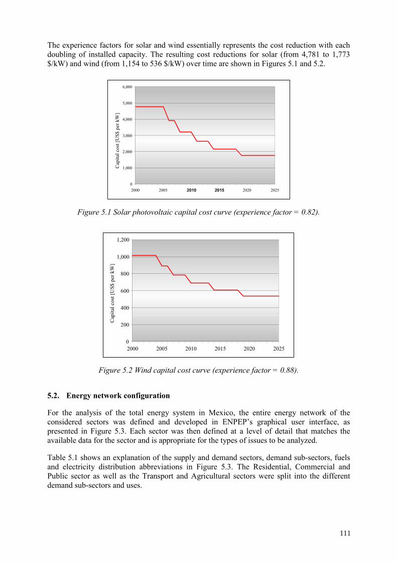
The experience factors for solar and wind essentially represents the cost reduction with each doubling of installed capacity. The resulting cost reductions for solar (from 4,781 to 1,773 $/kW) and wind (from 1,154 to 536 $/kW) over time are shown in Figures 5.1 and 5.2.

0

1,000

2,000

3,000

4,000

5,000

6,000

2000 2005 2010 2015 2020 2025

Cap

ital c

ost [

US$

per

kW

]

Figure 5.1 Solar photovoltaic capital cost curve (experience factor = 0.82).

0

200

400

600

800

1,000

1,200

2000 2005 2010 2015 2020 2025

Cap

ital c

ost [

US$

per

kW

]

Figure 5.2 Wind capital cost curve (experience factor = 0.88).

5.2. Energy network configuration

For the analysis of the total energy system in Mexico, the entire energy network of the considered sectors was defined and developed in ENPEP’s graphical user interface, as presented in Figure 5.3. Each sector was then defined at a level of detail that matches the available data for the sector and is appropriate for the types of issues to be analyzed.

Table 5.1 shows an explanation of the supply and demand sectors, demand sub-sectors, fuels and electricity distribution abbreviations in Figure 5.3. The Residential, Commercial and Public sector as well as the Transport and Agricultural sectors were split into the different demand sub-sectors and uses.

111

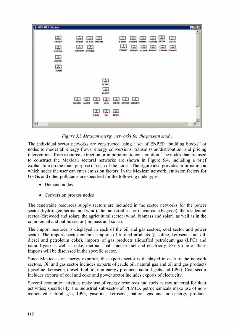
Figure 5.3 Mexican energy networks for the present study.

The individual sector networks are constructed using a set of ENPEP “building blocks” or nodes to model all energy flows, energy conversions, transmission/distribution, and pricing interventions from resource extraction or importation to consumption. The nodes that are used to construct the Mexican sectoral networks are shown in Figure 5.4, including a brief explanation on the main purpose of each of the nodes. The figure also provides information at which nodes the user can enter emission factors. In the Mexican network, emission factors for GHGs and other pollutants are specified for the following node types:

• Demand nodes

• Conversion process nodes

The renewable resources supply sectors are included in the sector networks for the power sector (hydro, geothermal and wind), the industrial sector (sugar cane bagasse), the residential sector (firewood and solar), the agricultural sector (wind, biomass and solar), as well as in the commercial and public sector (biomass and solar).

The import resource is displayed in each of the oil and gas sectors, coal sector and power sector. The imports sector contains imports of refined products (gasoline, kerosene, fuel oil, diesel and petroleum coke), imports of gas products (liquefied petroleum gas (LPG) and natural gas) as well as coke, thermal coal, nuclear fuel and electricity. Every one of these imports will be discussed in the specific sector.

Since Mexico is an energy exporter, the exports sector is displayed in each of the network sectors. Oil and gas sector includes exports of crude oil, natural gas and oil and gas products (gasoline, kerosene, diesel, fuel oil, non-energy products, natural gads and LPG). Coal sector includes exports of coal and coke and power sector includes exports of electricity.

Several economic activities make use of energy resources and fuels as raw material for their activities; specifically, the industrial sub-sector of PEMEX petrochemicals make use of non-associated natural gas, LPG, gasoline, kerosene, natural gas and non-energy products

112

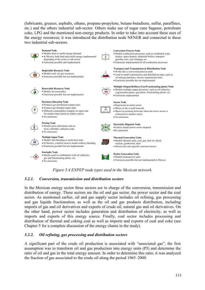
(lubricants, greases, asphalts, ethane, propane-propylene, butane-butadiene, sulfur, paraffines, etc.) and the others industrial sub-sector. Others make use of sugar cane bagasse, petroleum coke, LPG and the mentioned non-energy products. In order to take into account these uses of the energy resources; it was introduced the distribution node NENER and connected to these two industrial sub-sectors.

Demand Node • Models final or useful energy demand • In Mexico, both final and useful energy implemented

depending of the sector or sub-sector • Emissions possible and implemented

Conversion Process Node • Models combustion processes, such as residential water

heaters, space heaters, industrial boilers, transport gasoline cars, coal cleaning, etc.

• Emissions implemented for all combustion processes

Depletable Resource Node • Models coal, oil, gas resources • Emissions possible but not implemented

Transport and Transmission & Distribution Node • Works like a conversion process node • Used to model transmission and distribution steps, such as

oil and gas pipelines, electric transmission lines • Emissions possible but not implemented

Renewable Resource Node • Models all renewables • Emissions possible but not implemented

Multiple Output/Refinery/Gas/Fractionating plants Node • Models multiple output processes, such as oil refineries,

cogeneration plants, gas plants, fractionating plants, etc. • Emissions implemented

Pricing Node • Models price distortions such as

taxes, subsidies, and price caps • No emissions

Electricity Dispatch Node •Used to model power sector dispatch •No emissions

Decision/Allocation Node • Products get distributed (output side) • Products get blended (input side) • Different commodities compete on input side

for market share based on relative prices • No emissions

Sector Node • Represents an entire sector • Shows in the overall network • Shows in sectorial networks when the active sector is

connected to another sector • No emissions

Multiple Input Node • Models fuel blending or multi-fuel units • In Mexico, could be used to model refinery blending • Emissions possible but not implemented

Thermal Generation Units • Models thermal units, coal, gas, fuel oil, diesel,

nuclear, geothermal, dual • Mexico has unit-specific emission factors

Stockpile Node • Mostly used in combination with oil refineries,

gas and fractionating plants, etc. • No emissions

Hydro Generation Units • Models hydropower units • Emissions possible but not implemented in Mexico

Figure 5.4 ENPEP node types used in the Mexican network.

5.2.1. Conversion, transmission and distribution sectors

In the Mexican energy sector three sectors are in charge of the conversion, transmission and distribution of energy. These sectors are the oil and gas sector, the power sector and the coal sector. As mentioned earlier, oil and gas supply sector includes oil refining, gas processing and gas liquids fractionation, as well as the oil and gas products distribution, including imports of gas and oil derivatives and exports of crude oil, natural gas and oil derivatives. On the other hand, power sector includes generation and distribution of electricity, as well as imports and exports of this energy source. Finally, coal sector includes processing and distribution of thermal and coking coal as well as imports and exports of coal and coke (see Chapter 5 for a complete discussion of the energy chains in the study).

5.2.2. Oil refining, gas processing and distribution sectors

A significant part of the crude oil production is associated with “associated gas”, the first assumption was to transform oil and gas production into energy units (PJ) and determine the ratio of oil and gas in the total energy amount. In order to determine this ratio, it was analyzed the fraction of gas associated to the crude oil along the period 1965–2000.

113

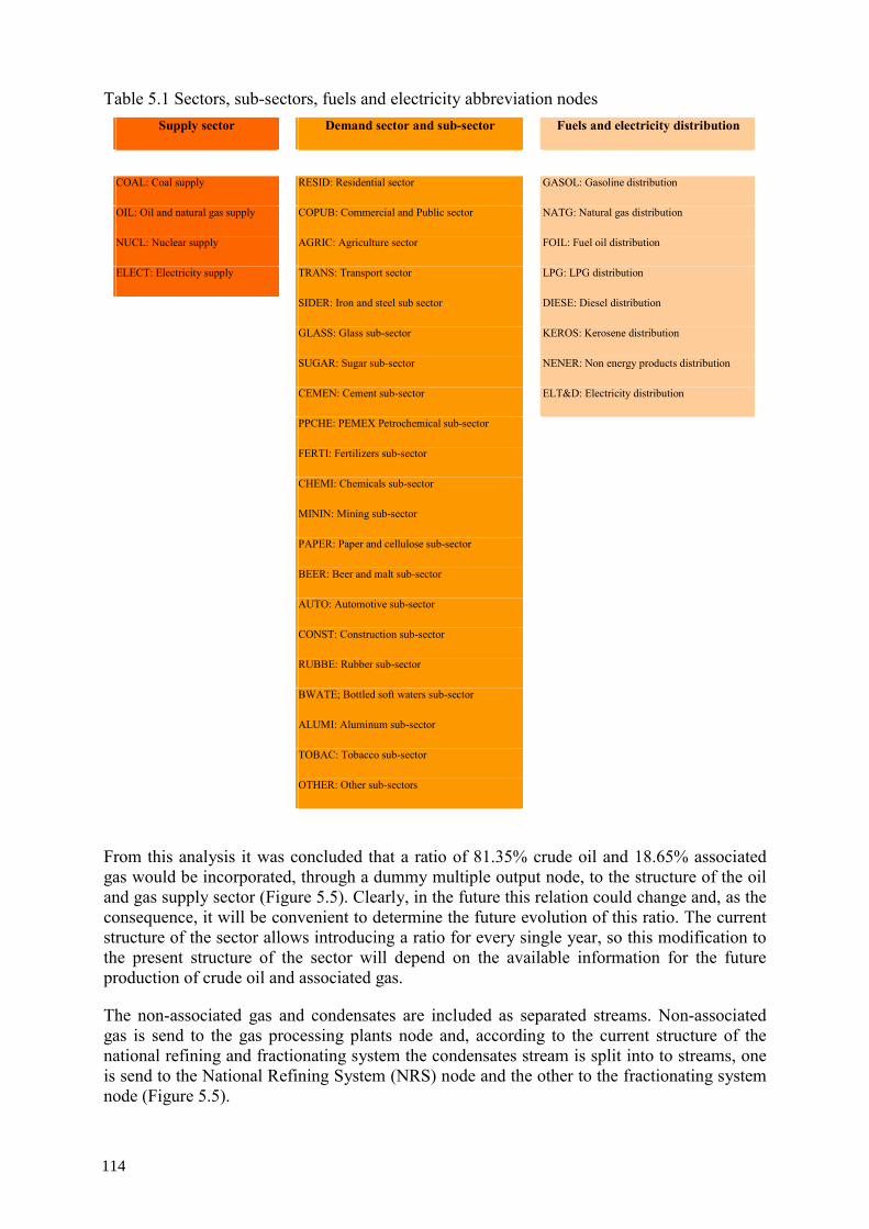
Table 5.1 Sectors, sub-sectors, fuels and electricity abbreviation nodes Supply sector Demand sector and sub-sector Fuels and electricity distribution

COAL: Coal supply RESID: Residential sector GASOL: Gasoline distribution

OIL: Oil and natural gas supply COPUB: Commercial and Public sector NATG: Natural gas distribution

NUCL: Nuclear supply AGRIC: Agriculture sector FOIL: Fuel oil distribution

ELECT: Electricity supply TRANS: Transport sector LPG: LPG distribution

SIDER: Iron and steel sub sector DIESE: Diesel distribution

GLASS: Glass sub-sector KEROS: Kerosene distribution

SUGAR: Sugar sub-sector NENER: Non energy products distribution

CEMEN: Cement sub-sector ELT&D: Electricity distribution

PPCHE: PEMEX Petrochemical sub-sector

FERTI: Fertilizers sub-sector

CHEMI: Chemicals sub-sector

MININ: Mining sub-sector

PAPER: Paper and cellulose sub-sector

BEER: Beer and malt sub-sector

AUTO: Automotive sub-sector

CONST: Construction sub-sector

RUBBE: Rubber sub-sector

BWATE; Bottled soft waters sub-sector

ALUMI: Aluminum sub-sector

TOBAC: Tobacco sub-sector

OTHER: Other sub-sectors

From this analysis it was concluded that a ratio of 81.35% crude oil and 18.65% associated gas would be incorporated, through a dummy multiple output node, to the structure of the oil and gas supply sector (Figure 5.5). Clearly, in the future this relation could change and, as the consequence, it will be convenient to determine the future evolution of this ratio. The current structure of the sector allows introducing a ratio for every single year, so this modification to the present structure of the sector will depend on the available information for the future production of crude oil and associated gas.

The non-associated gas and condensates are included as separated streams. Non-associated gas is send to the gas processing plants node and, according to the current structure of the national refining and fractionating system the condensates stream is split into to streams, one is send to the National Refining System (NRS) node and the other to the fractionating system node (Figure 5.5).

114

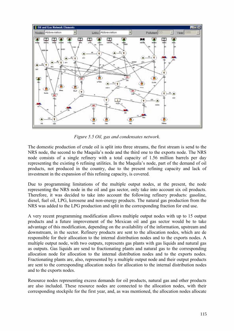
Figure 5.5 Oil, gas and condensates network.

The domestic production of crude oil is split into three streams, the first stream is send to the NRS node, the second to the Maquila’s node and the third one to the exports node. The NRS node consists of a single refinery with a total capacity of 1.56 million barrels per day representing the existing 6 refining utilities. In the Maquila’s node, part of the demand of oil products, not produced in the country, due to the present refining capacity and lack of investment in the expansion of this refining capacity, is covered.

Due to programming limitations of the multiple output nodes, at the present, the node representing the NRS node in the oil and gas sector, only take into account six oil products. Therefore, it was decided to take into account the following refinery products: gasoline, diesel, fuel oil, LPG, kerosene and non-energy products. The natural gas production from the NRS was added to the LPG production and split in the corresponding fraction for end use.

A very recent programming modification allows multiple output nodes with up to 15 output products and a future improvement of the Mexican oil and gas sector would be to take advantage of this modification, depending on the availability of the information, upstream and downstream, in the sector. Refinery products are sent to the allocation nodes, which are de responsible for their allocation to the internal distribution nodes and to the exports nodes. A multiple output node, with two outputs, represents gas plants with gas liquids and natural gas as outputs. Gas liquids are send to fractionating plants and natural gas to the corresponding allocation node for allocation to the internal distribution nodes and to the exports nodes. Fractionating plants are, also, represented by a multiple output node and their output products are sent to the corresponding allocation nodes for allocation to the internal distribution nodes and to the exports nodes.

Resource nodes representing excess demands for oil products, natural gas and other products are also included. These resource nodes are connected to the allocation nodes, with their corresponding stockpile for the first year, and, as was mentioned, the allocation nodes allocate

115

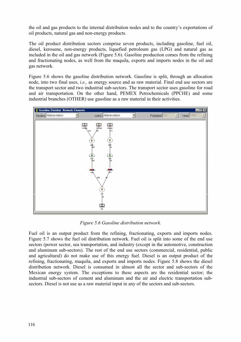
the oil and gas products to the internal distribution nodes and to the country’s exportations of oil products, natural gas and non-energy products.

The oil product distribution sectors comprise seven products, including gasoline, fuel oil, diesel, kerosene, non-energy products, liquefied petroleum gas (LPG) and natural gas as included in the oil and gas network (Figure 5.6). Gasoline production comes from the refining and fractionating nodes, as well from the maquila, exports and imports nodes in the oil and gas network.

Figure 5.6 shows the gasoline distribution network. Gasoline is split, through an allocation node, into two final uses, i.e., as energy source and as raw material. Final end use sectors are the transport sector and two industrial sub-sectors. The transport sector uses gasoline for road and air transportation. On the other hand, PEMEX Petrochemicals (PPCHE) and some industrial branches (OTHER) use gasoline as a raw material in their activities.

Figure 5.6 Gasoline distribution network.

Fuel oil is an output product from the refining, fractionating, exports and imports nodes. Figure 5.7 shows the fuel oil distribution network. Fuel oil is split into some of the end use sectors (power sector, sea transportation, and industry (except in the automotive, construction and aluminum sub-sectors). The rest of the end use sectors (commercial, residential, public and agricultural) do not make use of this energy fuel. Diesel is an output product of the refining, fractionating, maquila, and exports and imports nodes. Figure 5.8 shows the diesel distribution network. Diesel is consumed in almost all the sector and sub-sectors of the Mexican energy system. The exceptions to these aspects are the residential sector; the industrial sub-sectors of cement and aluminum and the air and electric transportation sub-sectors. Diesel is not use as a raw material input in any of the sectors and sub-sectors.

116

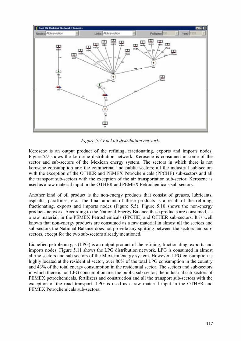
Figure 5.7 Fuel oil distribution network.

Kerosene is an output product of the refining, fractionating, exports and imports nodes. Figure 5.9 shows the kerosene distribution network. Kerosene is consumed in some of the sector and sub-sectors of the Mexican energy system. The sectors in which there is not kerosene consumption are: the commercial and public sectors; all the industrial sub-sectors with the exception of the OTHER and PEMEX Petrochemicals (PPCHE) sub-sectors and all the transport sub-sectors with the exception of the air transportation sub-sector. Kerosene is used as a raw material input in the OTHER and PEMEX Petrochemicals sub-sectors.

Another kind of oil product is the non-energy products that consist of greases, lubricants, asphalts, paraffines, etc. The final amount of these products is a result of the refining, fractionating, exports and imports nodes (Figure 5.5). Figure 5.10 shows the non-energy products network. According to the National Energy Balance these products are consumed, as a raw material, in the PEMEX Petrochemicals (PPCHE) and OTHER sub-sectors. It is well known that non-energy products are consumed as a raw material in almost all the sectors and sub-sectors the National Balance does not provide any splitting between the sectors and sub-sectors, except for the two sub-sectors already mentioned.

Liquefied petroleum gas (LPG) is an output product of the refining, fractionating, exports and imports nodes. Figure 5.11 shows the LPG distribution network. LPG is consumed in almost all the sectors and sub-sectors of the Mexican energy system. However, LPG consumption is highly located at the residential sector, over 80% of the total LPG consumption in the country and 43% of the total energy consumption in the residential sector. The sectors and sub-sectors in which there is not LPG consumption are: the public sub-sector; the industrial sub-sectors of PEMEX petrochemicals, fertilizers and construction and all the transport sub-sectors with the exception of the road transport. LPG is used as a raw material input in the OTHER and PEMEX Petrochemicals sub-sectors.

117

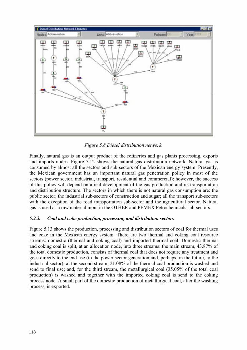
Figure 5.8 Diesel distribution network.

Finally, natural gas is an output product of the refineries and gas plants processing, exports and imports nodes. Figure 5.12 shows the natural gas distribution network. Natural gas is consumed by almost all the sectors and sub-sectors of the Mexican energy system. Presently, the Mexican government has an important natural gas penetration policy in most of the sectors (power sector, industrial, transport, residential and commercial); however, the success of this policy will depend on a real development of the gas production and its transportation and distribution structure. The sectors in which there is not natural gas consumption are: the public sector; the industrial sub-sectors of construction and sugar; all the transport sub-sectors with the exception of the road transportation sub-sector and the agricultural sector. Natural gas is used as a raw material input in the OTHER and PEMEX Petrochemicals sub-sectors.

5.2.3. Coal and coke production, processing and distribution sectors

Figure 5.13 shows the production, processing and distribution sectors of coal for thermal uses and coke in the Mexican energy system. There are two thermal and coking coal resource streams: domestic (thermal and coking coal) and imported thermal coal. Domestic thermal and coking coal is split, at an allocation node, into three streams: the main stream, 43.87% of the total domestic production, consists of thermal coal that does not require any treatment and goes directly to the end use (to the power sector generation and, perhaps, in the future, to the industrial sector); at the second stream, 21.08% of the thermal coal production is washed and send to final use; and, for the third stream, the metallurgical coal (35.05% of the total coal production) is washed and together with the imported coking coal is send to the coking process node. A small part of the domestic production of metallurgical coal, after the washing process, is exported.

118

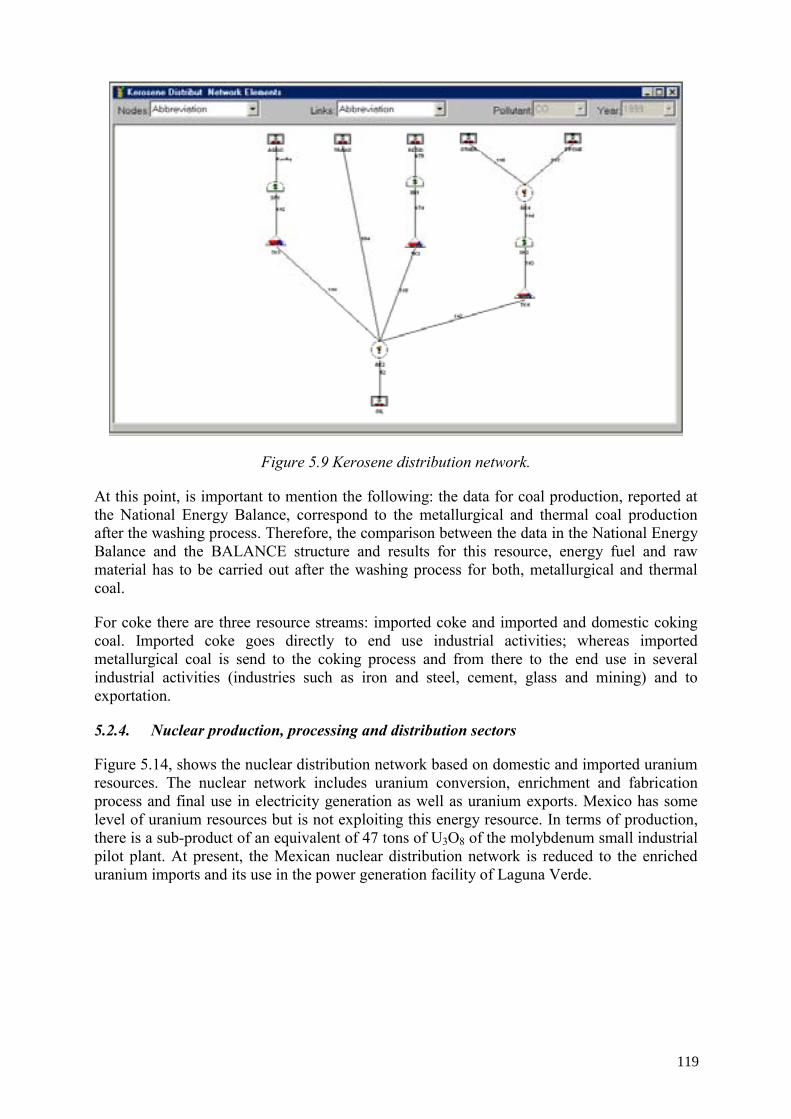
Figure 5.9 Kerosene distribution network.

At this point, is important to mention the following: the data for coal production, reported at the National Energy Balance, correspond to the metallurgical and thermal coal production after the washing process. Therefore, the comparison between the data in the National Energy Balance and the BALANCE structure and results for this resource, energy fuel and raw material has to be carried out after the washing process for both, metallurgical and thermal coal.

For coke there are three resource streams: imported coke and imported and domestic coking coal. Imported coke goes directly to end use industrial activities; whereas imported metallurgical coal is send to the coking process and from there to the end use in several industrial activities (industries such as iron and steel, cement, glass and mining) and to exportation.

5.2.4. Nuclear production, processing and distribution sectors

Figure 5.14, shows the nuclear distribution network based on domestic and imported uranium resources. The nuclear network includes uranium conversion, enrichment and fabrication process and final use in electricity generation as well as uranium exports. Mexico has some level of uranium resources but is not exploiting this energy resource. In terms of production, there is a sub-product of an equivalent of 47 tons of U3O8 of the molybdenum small industrial pilot plant. At present, the Mexican nuclear distribution network is reduced to the enriched uranium imports and its use in the power generation facility of Laguna Verde.

119

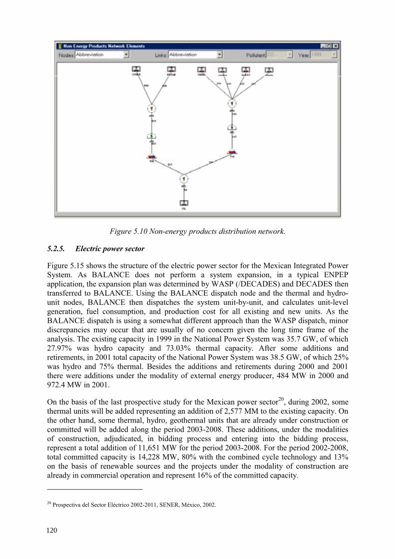
Figure 5.10 Non-energy products distribution network.

5.2.5. Electric power sector

Figure 5.15 shows the structure of the electric power sector for the Mexican Integrated Power System. As BALANCE does not perform a system expansion, in a typical ENPEP application, the expansion plan was determined by WASP (/DECADES) and DECADES then transferred to BALANCE. Using the BALANCE dispatch node and the thermal and hydro-unit nodes, BALANCE then dispatches the system unit-by-unit, and calculates unit-level generation, fuel consumption, and production cost for all existing and new units. As the BALANCE dispatch is using a somewhat different approach than the WASP dispatch, minor discrepancies may occur that are usually of no concern given the long time frame of the analysis. The existing capacity in 1999 in the National Power System was 35.7 GW, of which 27.97% was hydro capacity and 73.03% thermal capacity. After some additions and retirements, in 2001 total capacity of the National Power System was 38.5 GW, of which 25% was hydro and 75% thermal. Besides the additions and retirements during 2000 and 2001 there were additions under the modality of external energy producer, 484 MW in 2000 and 972.4 MW in 2001.

On the basis of the last prospective study for the Mexican power sector20, during 2002, some thermal units will be added representing an addition of 2,577 MM to the existing capacity. On the other hand, some thermal, hydro, geothermal units that are already under construction or committed will be added along the period 2003-2008. These additions, under the modalities of construction, adjudicated, in bidding process and entering into the bidding process, represent a total addition of 11,651 MW for the period 2003-2008. For the period 2002-2008, total committed capacity is 14,228 MW, 80% with the combined cycle technology and 13% on the basis of renewable sources and the projects under the modality of construction are already in commercial operation and represent 16% of the committed capacity.

20 Prospectiva del Sector Eléctrico 2002-2011, SENER, México, 2002.

120

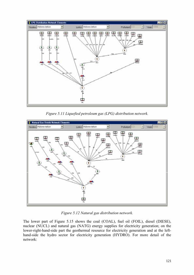
Figure 5.11 Liquefied petroleum gas (LPG) distribution network.

Figure 5.12 Natural gas distribution network.

The lower part of Figure 5.15 shows the coal (COAL), fuel oil (FOIL), diesel (DIESE), nuclear (NUCL) and natural gas (NATG) energy supplies for electricity generation; on the lower-right-hand-side part the geothermal resource for electricity generation and at the left-hand-side the hydro sector for electricity generation (HYDRO). For more detail of the network:

121

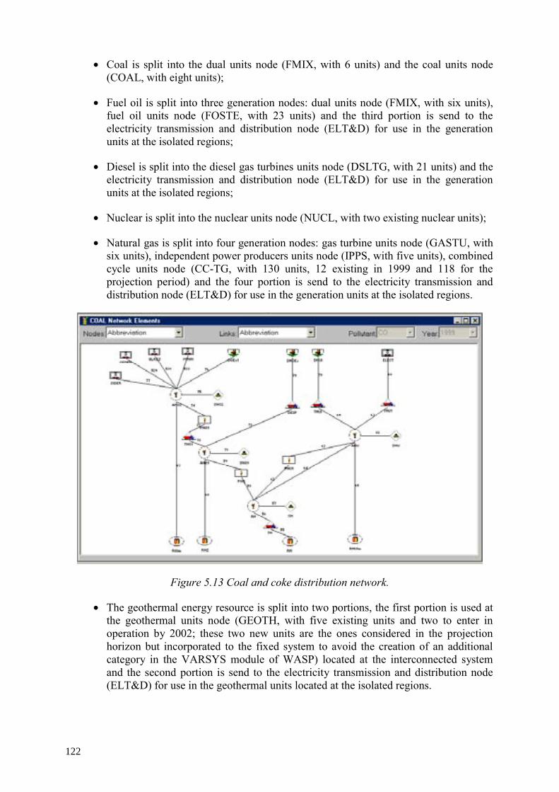
• Coal is split into the dual units node (FMIX, with 6 units) and the coal units node (COAL, with eight units);

• Fuel oil is split into three generation nodes: dual units node (FMIX, with six units), fuel oil units node (FOSTE, with 23 units) and the third portion is send to the electricity transmission and distribution node (ELT&D) for use in the generation units at the isolated regions;

• Diesel is split into the diesel gas turbines units node (DSLTG, with 21 units) and the electricity transmission and distribution node (ELT&D) for use in the generation units at the isolated regions;

• Nuclear is split into the nuclear units node (NUCL, with two existing nuclear units);

• Natural gas is split into four generation nodes: gas turbine units node (GASTU, with six units), independent power producers units node (IPPS, with five units), combined cycle units node (CC-TG, with 130 units, 12 existing in 1999 and 118 for the projection period) and the four portion is send to the electricity transmission and distribution node (ELT&D) for use in the generation units at the isolated regions.

Figure 5.13 Coal and coke distribution network.

• The geothermal energy resource is split into two portions, the first portion is used at the geothermal units node (GEOTH, with five existing units and two to enter in operation by 2002; these two new units are the ones considered in the projection horizon but incorporated to the fixed system to avoid the creation of an additional category in the VARSYS module of WASP) located at the interconnected system and the second portion is send to the electricity transmission and distribution node (ELT&D) for use in the geothermal units located at the isolated regions.

122

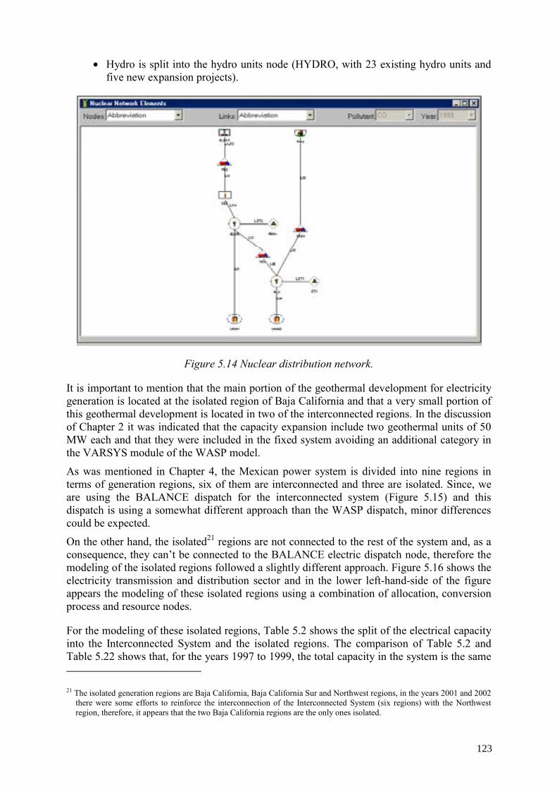
• Hydro is split into the hydro units node (HYDRO, with 23 existing hydro units and five new expansion projects).

Figure 5.14 Nuclear distribution network.

It is important to mention that the main portion of the geothermal development for electricity generation is located at the isolated region of Baja California and that a very small portion of this geothermal development is located in two of the interconnected regions. In the discussion of Chapter 2 it was indicated that the capacity expansion include two geothermal units of 50 MW each and that they were included in the fixed system avoiding an additional category in the VARSYS module of the WASP model.

As was mentioned in Chapter 4, the Mexican power system is divided into nine regions in terms of generation regions, six of them are interconnected and three are isolated. Since, we are using the BALANCE dispatch for the interconnected system (Figure 5.15) and this dispatch is using a somewhat different approach than the WASP dispatch, minor differences could be expected.

On the other hand, the isolated21 regions are not connected to the rest of the system and, as a consequence, they can’t be connected to the BALANCE electric dispatch node, therefore the modeling of the isolated regions followed a slightly different approach. Figure 5.16 shows the electricity transmission and distribution sector and in the lower left-hand-side of the figure appears the modeling of these isolated regions using a combination of allocation, conversion process and resource nodes.

For the modeling of these isolated regions, Table 5.2 shows the split of the electrical capacity into the Interconnected System and the isolated regions. The comparison of Table 5.2 and Table 5.22 shows that, for the years 1997 to 1999, the total capacity in the system is the same 21 The isolated generation regions are Baja California, Baja California Sur and Northwest regions, in the years 2001 and 2002

there were some efforts to reinforce the interconnection of the Interconnected System (six regions) with the Northwest region, therefore, it appears that the two Baja California regions are the only ones isolated.

123

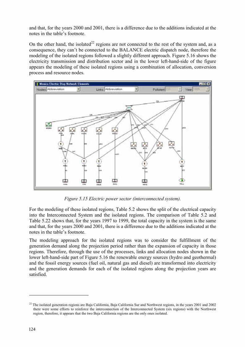
and that, for the years 2000 and 2001, there is a difference due to the additions indicated at the notes in the table’s footnote.

On the other hand, the isolated22 regions are not connected to the rest of the system and, as a consequence, they can’t be connected to the BALANCE electric dispatch node, therefore the modeling of the isolated regions followed a slightly different approach. Figure 5.16 shows the electricity transmission and distribution sector and in the lower left-hand-side of the figure appears the modeling of these isolated regions using a combination of allocation, conversion process and resource nodes.

Figure 5.15 Electric power sector (interconnected system).

For the modeling of these isolated regions, Table 5.2 shows the split of the electrical capacity into the Interconnected System and the isolated regions. The comparison of Table 5.2 and Table 5.22 shows that, for the years 1997 to 1999, the total capacity in the system is the same and that, for the years 2000 and 2001, there is a difference due to the additions indicated at the notes in the table’s footnote.

The modeling approach for the isolated regions was to consider the fulfillment of the generation demand along the projection period rather than the expansion of capacity in those regions. Therefore, through the use of the processes, links and allocation nodes shown in the lower left-hand-side part of Figure 5.16 the renewable energy sources (hydro and geothermal) and the fossil energy sources (fuel oil, natural gas and diesel) are transformed into electricity and the generation demands for each of the isolated regions along the projection years are satisfied.

22 The isolated generation regions are Baja California, Baja California Sur and Northwest regions, in the years 2001 and 2002

there were some efforts to reinforce the interconnection of the Interconnected System (six regions) with the Northwest region, therefore, it appears that the two Baja California regions are the only ones isolated.

124

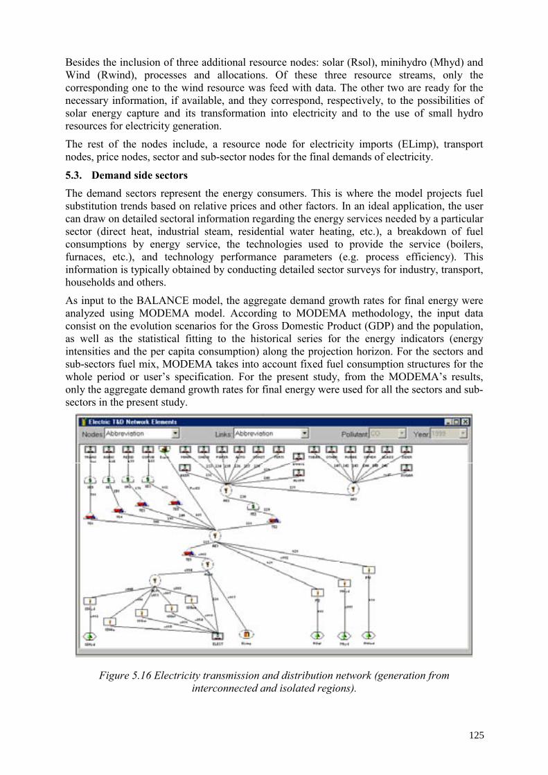
Besides the inclusion of three additional resource nodes: solar (Rsol), minihydro (Mhyd) and Wind (Rwind), processes and allocations. Of these three resource streams, only the corresponding one to the wind resource was feed with data. The other two are ready for the necessary information, if available, and they correspond, respectively, to the possibilities of solar energy capture and its transformation into electricity and to the use of small hydro resources for electricity generation.

The rest of the nodes include, a resource node for electricity imports (ELimp), transport nodes, price nodes, sector and sub-sector nodes for the final demands of electricity.

5.3. Demand side sectors The demand sectors represent the energy consumers. This is where the model projects fuel substitution trends based on relative prices and other factors. In an ideal application, the user can draw on detailed sectoral information regarding the energy services needed by a particular sector (direct heat, industrial steam, residential water heating, etc.), a breakdown of fuel consumptions by energy service, the technologies used to provide the service (boilers, furnaces, etc.), and technology performance parameters (e.g. process efficiency). This information is typically obtained by conducting detailed sector surveys for industry, transport, households and others.

As input to the BALANCE model, the aggregate demand growth rates for final energy were analyzed using MODEMA model. According to MODEMA methodology, the input data consist on the evolution scenarios for the Gross Domestic Product (GDP) and the population, as well as the statistical fitting to the historical series for the energy indicators (energy intensities and the per capita consumption) along the projection horizon. For the sectors and sub-sectors fuel mix, MODEMA takes into account fixed fuel consumption structures for the whole period or user’s specification. For the present study, from the MODEMA’s results, only the aggregate demand growth rates for final energy were used for all the sectors and sub-sectors in the present study.

Figure 5.16 Electricity transmission and distribution network (generation from interconnected and isolated regions).

125

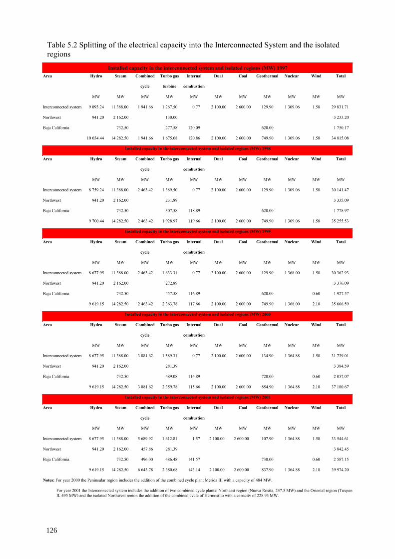
Table 5.2 Splitting of the electrical capacity into the Interconnected System and the isolated regions

Installed capacity in the interconnected system and isolated regions (MW) 1997 Area Hydro Steam Combined Turbo gas Internal Dual Coal Geothermal Nuclear Wind Total

cycle turbine combustion

MW MW MW MW MW MW MW MW MW MW MW

Interconnected system 9 093.24 11 388.00 1 941.66 1 267.50 0.77 2 100.00 2 600.00 129.90 1 309.06 1.58 29 831.71

Northwest 941.20 2 162.00 130.00 3 233.20

Baja California 732.50 277.58 120.09 620.00 1 750.17

10 034.44 14 282.50 1 941.66 1 675.08 120.86 2 100.00 2 600.00 749.90 1 309.06 1.58 34 815.08

Installed capacity in the interconnected system and isolated regions (MW) 1998

Area Hydro Steam Combined Turbo gas Internal Dual Coal Geothermal Nuclear Wind Total

cycle combustion



Northwest 941.20 2 162.00 231.89 3 335.09

Baja California 732.50 307.58 118.89 620.00 1 778.97

9 700.44 14 282.50 2 463.42 1 928.97 119.66 2 100.00 2 600.00 749.90 1 309.06 1.58 35 255.53



cycle combustion



Northwest 941.20 2 162.00 272.89 3 376.09

Baja California 732.50 457.58 116.89 620.00 0.60 1 927.57

9 619.15 14 282.50 2 463.42 2 363.78 117.66 2 100.00 2 600.00 749.90 1 368.00 2.18 35 666.59



cycle combustion



Northwest 941.20 2 162.00 281.39 3 384.59

Baja California 732.50 489.08 114.89 720.00 0.60 2 057.07

9 619.15 14 282.50 3 881.62 2 359.78 115.66 2 100.00 2 600.00 854.90 1 364.88 2.18 37 180.67



cycle combustion



Northwest 941.20 2 162.00 457.86 281.39 3 842.45

Baja California 732.50 496.00 486.48 141.57 730.00 0.60 2 587.15

9 619.15 14 282.50 6 643.78 2 380.68 143.14 2 100.00 2 600.00 837.90 1 364.88 2.18 39 974.20

Notes: For year 2000 the Peninsular region includes the addition of the combined cycle plant Mérida III with a capacity of 484 MW.

For year 2001 the Interconnected system includes the addition of two combined cycle plants: Northeast region (Nueva Rosita, 247.5 MW) and the Oriental region (Tuxpan II, 495 MW) and the isolated Northwest region the addition of the combined cycle of Hermosillo with a capacity of 228.93 MW.

126

Table 5.3 shows the growth rates structure, in terms of Great Divisions and Divisions, for the GDP scenario along the projection horizon. The projection horizon was divided into two parts, the first one from 2002 to 2011 with an annual average growth rate of 4.5% and the second one from 2012 to 2025 with and annual average growth rate of 3.5%. The Secretaría de Energía provided the first part, while the working team, considering the GDP annual average growth rate for the last 25 years, determined the second.

Table 5.4 shows the considered evolution scenario for the country’s population. This population scenario corresponds to the medium projection of the Consejo Nacional de Población (CONAPO).

The annual demand growth rates for final energy, for the sectors and sub-sectors considered in the study, are shown in Tables 5.5, 5.6, 5.7 and 5.8. The demand growth rates are inputs for the demand nodes. The fuel choices in each sector and sub-sector come from the National Energy Balances. The team members based on their insights and information on the individual sectors and sub-sectors determined fuel substitution possibilities, that is, the network structure for each sector and sub-sector.

In the case of Mexico, no information was available on the specification of the energy services and technologies; however, some of the industrial sub-sectors were split into specific energy services by considering international data for process efficiencies. The remaining industrial demand sectors are, therefore, implemented at a final energy level. That is, energy services are not considered for these sub-sectors, and the fuel competition is based mostly on fuel prices. For all industrial sub-sectors a breakdown of fuel consumptions was carried out. For the transport sector the breakdown was performed in terms of the five sub-sectors discussed in the Summary, section 5.3. For the road sub-sector, the energy services approach is considered through the process efficiencies and the hybrid option. For the remaining transport sub-sectors the demand is implemented at a final energy level.

5.3.1. Industrial demand sector The Mexican industrial sector is highly energy intensive and efficiency of main conversion processes used in this sector is still below that of other industrialized countries so it is expected that industrial energy consumption will increase importantly. In order to estimate future industrial energy demand in the model, the study was conducted with 17 industrial sub-sectors (Table 5.1) as it is presented in the National Energy Balance (PEMEX petrochemicals, iron and steel, cement, sugar, glass, chemicals, malt and beer, automotive, paper and cellulose, rubber, tobacco, aluminum, bottled waters, fertilizers, mining and others).

Apart from electricity growth rates which are calculated taking into account assumptions of the WASP run, the rest fuel growth rates for industrial sub-sectors comes from the MODEMA model assuming fixed structures for the whole period for every one of them. This growth rates also take into account specific policies as environmental restrictions aiming to reduce drastically the consumption of fuel oil in the industrial sector for the year 2006. While no significant policies aimed to promote renewable energy penetration are visualized in this sector, cogeneration development is carefully taken into account in the design of the industrial sector network.

Considering the limitations on information on the specification of the energy services and technologies, the energy consumption in this sector has been analyzed in detail only for five individual industrial branches. These sub-sectors are iron and steel, PEMEX-petrochemicals, sugar, glass and cement. In those sub-sectors fuel consumption is represented considering the needs of heat, steam and electricity and the different technologies used to provide these

127

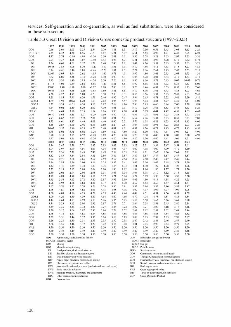
services. Self-generation and co-generation, as well as fuel substitution, were also considered in those sub-sectors.

Table 5.3 Great Division and Division Gross domestic product structure (1997–2025) 1997 1998 1999 2000 2001 2002 2003 2004 2005 2006 2007 2008 2009 2010 2011

GD1 0.16 3.03 2.03 3.35 2.54 0.70 1.81 1.31 3.17 0.56 0.51 5.43 3.05 3.63 3.21 INDUST 9.25 6.32 4.20 6.56 -3.51 1.87 5.21 5.97 6.51 6.63 4.95 4.91 6.48 6.75 6.23 GD2 4.47 2.74 -2.09 4.03 -0.56 2.30 2.41 3.01 3.36 2.78 3.21 3.03 2.95 3.23 3.31 GD3 9.94 7.37 4.18 7.07 -3.90 1.43 4.98 5.71 6.31 6.52 4.98 4.78 6.10 6.32 5.72

DI 3.24 6.60 4.01 3.57 1.79 2.40 2.40 2.61 3.47 4.26 3.51 3.63 3.55 3.63 3.21 DII 10.45 3.85 3.05 5.30 -10.13 -3.80 3.51 3.91 5.17 4.66 4.11 4.33 5.15 5.23 4.81 DIII 6.74 4.41 0.46 1.05 -4.46 -2.20 1.81 2.31 2.27 2.96 2.61 2.43 2.45 2.53 2.11 DIV 12.69 5.95 4.94 2.62 -4.05 -1.60 3.71 4.01 3.97 4.86 3.61 2.93 2.65 1.73 1.31 DV 6.82 6.06 2.36 3.13 -4.28 1.10 3.90 4.31 5.06 4.78 4.01 3.33 4.15 4.33 4.11 DVI 5.93 5.20 1.80 5.85 -4.24 3.50 7.20 8.61 8.86 8.06 5.71 5.43 9.05 10.03 9.71 DVII 11.13 4.00 0.39 3.58 -5.66 -1.40 5.81 5.81 5.97 5.66 4.31 4.03 6.35 6.43 6.01 DVIII 19.06 11.48 6.88 13.90 -6.22 2.80 7.80 8.91 9.26 9.46 6.81 6.53 8.55 8.73 7.61 DIX 10.46 7.88 5.66 12.16 -0.65 1.60 3.81 5.51 5.17 5.06 3.61 3.43 4.85 5.03 4.61

GD4 9.28 4.22 4.99 5.00 -4.51 3.70 7.30 8.31 8.56 8.56 5.31 5.83 9.45 9.83 9.41 GD5 5.21 1.85 7.91 6.20 1.71 2.46 4.95 5.47 5.94 5.65 4.78 5.22 5.46 5.59 5.10

GD5.1 4.89 1.93 10.69 6.20 1.53 2.02 4.96 5.57 5.93 5.94 4.84 4.97 5.30 5.41 5.00 GD5.2 6.22 5.39 -6.21 6.20 3.10 2.87 7.14 8.16 7.80 7.95 6.60 6.44 7.00 7.28 5.88 Gd5.3 6.14 0.02 2.40 6.20 2.00 4.30 4.01 3.91 5.17 3.26 3.61 5.83 5.45 5.63 5.21

SERV 6.55 4.69 3.80 7.35 1.14 1.86 3.98 4.60 4.81 5.09 4.44 4.42 4.51 4.65 4.43 GD6 10.70 5.64 3.45 11.07 -1.29 0.50 4.40 4.91 4.56 4.78 4.91 4.23 3.85 3.93 3.51 GD7 9.93 6.67 7.79 12.68 2.81 3.00 4.91 6.01 6.67 7.26 5.41 6.23 8.35 8.23 7.81 GD8 3.73 4.61 3.87 4.49 4.09 4.40 4.90 5.51 5.76 6.08 4.81 4.53 4.35 4.43 4.01 GD9 3.35 2.87 2.10 2.96 0.51 0.60 2.20 2.61 3.06 3.08 2.91 3.23 2.65 2.93 3.21 SBI 10.63 5.57 5.86 6.25 6.23 5.40 4.01 4.61 4.87 4.76 4.21 4.43 4.75 4.93 4.51 VAB 6.78 5.02 3.75 6.92 -0.26 1.69 4.20 4.80 5.20 5.30 4.40 4.61 5.01 5.21 4.91 IMP 6.70 5.10 3.75 6.92 -0.28 1.69 4.20 4.80 5.20 5.30 4.40 4.60 5.00 5.20 4.90 GDP 6.77 5.03 3.75 6.92 -0.26 1.69 4.20 4.80 5.20 5.30 4.40 4.61 5.01 5.21 4.91

2012 2013 2014 2015 2016 2017 2018 2019 2020 2021 2022 2023 2024 2025 GD1 2.34 2.47 2.59 2.71 2.82 2.93 3.03 3.13 3.22 3.31 3.39 3.47 3.54 3.61 INDUST 3.94 3.97 3.99 4.01 4.03 4.04 4.05 4.07 4.07 4.08 4.09 4.09 4.10 4.10 GD2 2.33 2.36 2.39 2.43 2.46 2.49 2.52 2.55 2.58 2.61 2.63 2.66 2.69 2.71 GD3 3.82 3.83 3.84 3.84 3.85 3.86 3.86 3.87 3.87 3.87 3.87 3.87 3.87 3.87

DI 2.74 2.71 2.68 2.65 2.62 2.59 2.57 2.54 2.52 2.50 2.48 2.47 2.45 2.44 DII 2.74 2.85 2.96 3.06 3.16 3.25 3.33 3.41 3.49 3.56 3.62 3.68 3.74 3.79 DIII 1.42 1.41 1.39 1.38 1.37 1.35 1.34 1.33 1.31 1.30 1.29 1.28 1.27 1.26 DIV 2.23 2.18 2.13 2.09 2.04 2.00 1.96 1.92 1.88 1.84 1.80 1.77 1.73 1.70 DV 2.89 2.92 2.94 2.96 2.98 3.01 3.03 3.04 3.06 3.08 3.10 3.12 3.13 3.15 DVI 4.79 4.89 4.98 5.05 5.11 5.17 5.21 5.24 5.27 5.29 5.30 5.30 5.30 5.30 DVII 3.45 3.54 3.63 3.72 3.80 3.87 3.93 3.99 4.05 4.10 4.14 4.18 4.22 4.25 DVIII 4.96 4.92 4.88 4.84 4.81 4.77 4.73 4.70 4.67 4.63 4.60 4.57 4.54 4.51 DIX 3.67 3.70 3.72 3.74 3.76 3.78 3.80 3.81 3.83 3.84 3.85 3.86 3.87 3.87

GD4 4.75 4.81 4.85 4.88 4.91 4.93 4.95 4.96 4.97 4.97 4.97 4.97 4.96 4.95 GD5 4.00 4.08 4.16 4.23 4.29 4.35 4.40 4.44 4.48 4.51 4.54 4.56 4.58 4.59

GD5.1 4.09 4.20 4.30 4.39 4.47 4.54 4.60 4.66 4.70 4.74 4.78 4.81 4.83 4.84 GD5.2 4.44 4.64 4.83 4.99 5.13 5.26 5.36 5.45 5.52 5.58 5.63 5.66 5.69 5.70 Gd5.3 3.34 3.23 3.13 3.04 2.95 2.87 2.79 2.71 2.64 2.58 2.51 2.45 2.40 2.34

SERV 3.39 3.36 3.34 3.32 3.29 3.27 3.26 3.24 3.22 3.21 3.20 3.18 3.17 3.16 GD6 3.20 3.12 3.04 2.97 2.90 2.84 2.78 2.72 2.67 2.62 2.57 2.52 2.48 2.44 GD7 4.75 4.78 4.81 4.83 4.84 4.85 4.86 4.86 4.86 4.86 4.85 4.84 4.83 4.82 GD8 3.59 3.51 3.44 3.37 3.30 3.24 3.18 3.13 3.08 3.03 2.99 2.95 2.91 2.87 GD9 2.26 2.28 2.30 2.31 2.33 2.35 2.37 2.38 2.40 2.42 2.44 2.46 2.47 2.49 SBI 3.66 3.56 3.46 3.37 3.29 3.22 3.14 3.08 3.01 2.95 2.90 2.84 2.79 2.75 VAB 3.50 3.50 3.50 3.50 3.50 3.50 3.50 3.50 3.50 3.50 3.50 3.50 3.50 3.50 IMP 3.50 3.49 3.49 3.49 3.49 3.49 3.49 3.49 3.49 3.49 3.49 3.49 3.49 3.48 GDP 3.50 3.50 3.50 3.50 3.50 3.50 3.50 3.50 3.50 3.50 3.50 3.50 3.50 3.50 GD1 Agriculture, silviculture and fishery GD5 Electricity, dry gas and water INDUST Industrial sector GD5.1 Electricity GD2 Mining GD5.2 Dry gas GD3 Manufacturing industry Gd5.3 Potable water DI Food products, drinks and tobacco SERV Services sector DII Textiles, clothes and leather products GD6 Commerce, restaurants and hotels DIII Wood industry and wood products GD7 Transport, storage and communications DIV Paper, paper products, printing and editing GD8 Financial services, insurance, real state and leasing DV Chemicals, oil, plastic and rubber GD9 Social, personal and community services DVI Non metallic mineral products (excludes oil and coal prods) SBI Banking services DVII Basic metallic industries VAB Gross aggregated value DVIII Metallic products, machinery and equipment IMP Taxes to the products, net subsides DIX Other manufacturing industries GDP Gross Domestic Product GD4 Construction

128

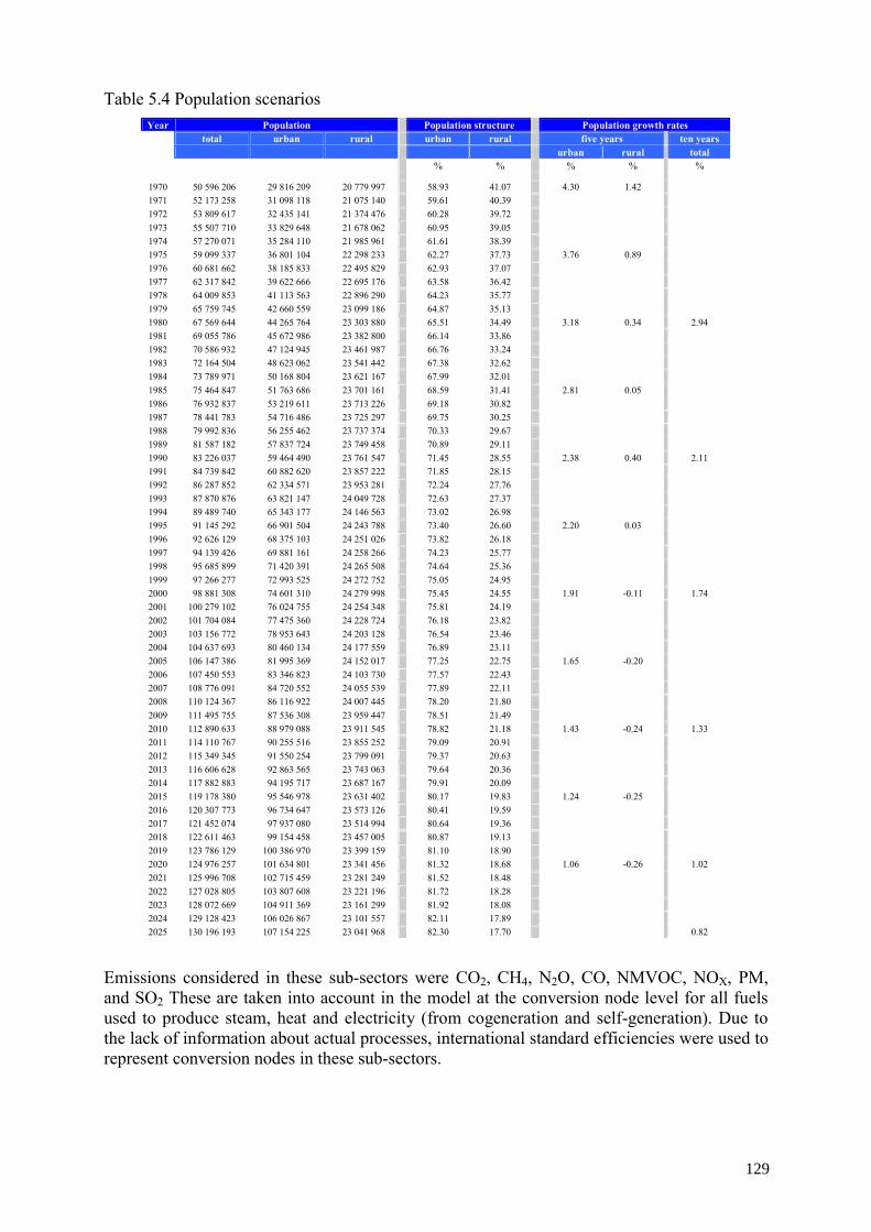
Table 5.4 Population scenarios Year Population Population structure Population growth rates

total urban rural urban rural five years ten years urban rural total

% % % % %

1970 50 596 206 29 816 209 20 779 997 58.93 41.07 4.30 1.42 1971 52 173 258 31 098 118 21 075 140 59.61 40.39 1972 53 809 617 32 435 141 21 374 476 60.28 39.72 1973 55 507 710 33 829 648 21 678 062 60.95 39.05 1974 57 270 071 35 284 110 21 985 961 61.61 38.39 1975 59 099 337 36 801 104 22 298 233 62.27 37.73 3.76 0.89 1976 60 681 662 38 185 833 22 495 829 62.93 37.07 1977 62 317 842 39 622 666 22 695 176 63.58 36.42 1978 64 009 853 41 113 563 22 896 290 64.23 35.77 1979 65 759 745 42 660 559 23 099 186 64.87 35.13 1980 67 569 644 44 265 764 23 303 880 65.51 34.49 3.18 0.34 2.94 1981 69 055 786 45 672 986 23 382 800 66.14 33.86 1982 70 586 932 47 124 945 23 461 987 66.76 33.24 1983 72 164 504 48 623 062 23 541 442 67.38 32.62 1984 73 789 971 50 168 804 23 621 167 67.99 32.01 1985 75 464 847 51 763 686 23 701 161 68.59 31.41 2.81 0.05 1986 76 932 837 53 219 611 23 713 226 69.18 30.82 1987 78 441 783 54 716 486 23 725 297 69.75 30.25 1988 79 992 836 56 255 462 23 737 374 70.33 29.67 1989 81 587 182 57 837 724 23 749 458 70.89 29.11 1990 83 226 037 59 464 490 23 761 547 71.45 28.55 2.38 0.40 2.11 1991 84 739 842 60 882 620 23 857 222 71.85 28.15 1992 86 287 852 62 334 571 23 953 281 72.24 27.76 1993 87 870 876 63 821 147 24 049 728 72.63 27.37 1994 89 489 740 65 343 177 24 146 563 73.02 26.98 1995 91 145 292 66 901 504 24 243 788 73.40 26.60 2.20 0.03 1996 92 626 129 68 375 103 24 251 026 73.82 26.18 1997 94 139 426 69 881 161 24 258 266 74.23 25.77 1998 95 685 899 71 420 391 24 265 508 74.64 25.36 1999 97 266 277 72 993 525 24 272 752 75.05 24.95 2000 98 881 308 74 601 310 24 279 998 75.45 24.55 1.91 -0.11 1.74 2001 100 279 102 76 024 755 24 254 348 75.81 24.19 2002 101 704 084 77 475 360 24 228 724 76.18 23.82 2003 103 156 772 78 953 643 24 203 128 76.54 23.46 2004 104 637 693 80 460 134 24 177 559 76.89 23.11 2005 106 147 386 81 995 369 24 152 017 77.25 22.75 1.65 -0.20 2006 107 450 553 83 346 823 24 103 730 77.57 22.43 2007 108 776 091 84 720 552 24 055 539 77.89 22.11 2008 110 124 367 86 116 922 24 007 445 78.20 21.80 2009 111 495 755 87 536 308 23 959 447 78.51 21.49 2010 112 890 633 88 979 088 23 911 545 78.82 21.18 1.43 -0.24 1.33 2011 114 110 767 90 255 516 23 855 252 79.09 20.91 2012 115 349 345 91 550 254 23 799 091 79.37 20.63 2013 116 606 628 92 863 565 23 743 063 79.64 20.36 2014 117 882 883 94 195 717 23 687 167 79.91 20.09 2015 119 178 380 95 546 978 23 631 402 80.17 19.83 1.24 -0.25 2016 120 307 773 96 734 647 23 573 126 80.41 19.59 2017 121 452 074 97 937 080 23 514 994 80.64 19.36 2018 122 611 463 99 154 458 23 457 005 80.87 19.13 2019 123 786 129 100 386 970 23 399 159 81.10 18.90 2020 124 976 257 101 634 801 23 341 456 81.32 18.68 1.06 -0.26 1.02 2021 125 996 708 102 715 459 23 281 249 81.52 18.48 2022 127 028 805 103 807 608 23 221 196 81.72 18.28 2023 128 072 669 104 911 369 23 161 299 81.92 18.08 2024 129 128 423 106 026 867 23 101 557 82.11 17.89 2025 130 196 193 107 154 225 23 041 968 82.30 17.70 0.82

Emissions considered in these sub-sectors were CO2, CH4, N2O, CO, NMVOC, NOX, PM, and SO2 These are taken into account in the model at the conversion node level for all fuels used to produce steam, heat and electricity (from cogeneration and self-generation). Due to the lack of information about actual processes, international standard efficiencies were used to represent conversion nodes in these sub-sectors.

129

This choice has been made considering the following criteria:

• The total fuel consumption;

• The natural gas consumption;

• The potential self-generation and co-generation development; and,

• The expected technological improvements that could lead to energy substitution.

In 1999 the five sub-sectors selected accounted for 50% of the total industrial fuel consumption and for 58% of the total industrial consumption of natural gas. In the same year almost 90% cogeneration and self-generation plants were located in these sub-sectors. We may also notice that iron and steel, glass, and cement sectors are the most technologically advanced in energy terms with good possibilities for fuel substitution and efficiency improvements.

In the cement sector (Figure 5.17) heat production is shifting from fuel oil consumption to alternative fuels such as used lubricants, used tires, etc. and some non-energy products and coke with important improvements in energy efficiency.

In the iron and steel sub-sector (Figure 5.18) we may notice more efficient electric furnaces that are being used since the nineties and the development of important cogeneration projects.

The case of the sugar sub-sector (Figure 5.19) is also relevant considering the high potential of biomass used for cogeneration and important needs of investments in order to improve energy efficiency.

The glass sub-sector (Figure 5.20) shows very efficient conversion processes that make the Mexican glass industry one of the most energy efficient industries in the world. This is also true in terms of quality and market penetration of its products that have contributed to the very successful expansion of this industry inside and outside the country providing this industry with significant net profits and financial soundness. Due to this situation energy efficiency and self-generation projects have been developed relatively more easily than in other sectors.

130

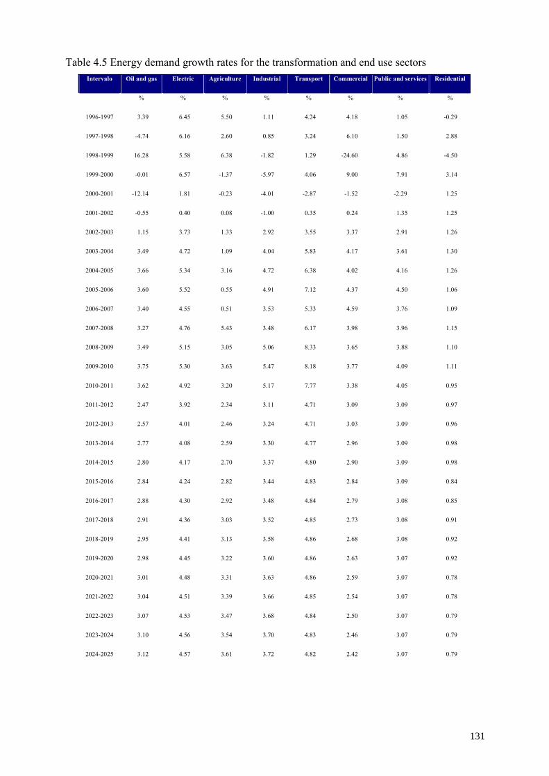
Table 4.5 Energy demand growth rates for the transformation and end use sectors Intervalo Oil and gas Electric Agriculture Industrial Transport Commercial Public and services Residential

% % % % % % % %

1996-1997 3.39 6.45 5.50 1.11 4.24 4.18 1.05 -0.29

1997-1998 -4.74 6.16 2.60 0.85 3.24 6.10 1.50 2.88

1998-1999 16.28 5.58 6.38 -1.82 1.29 -24.60 4.86 -4.50

1999-2000 -0.01 6.57 -1.37 -5.97 4.06 9.00 7.91 3.14

2000-2001 -12.14 1.81 -0.23 -4.01 -2.87 -1.52 -2.29 1.25

2001-2002 -0.55 0.40 0.08 -1.00 0.35 0.24 1.35 1.25

2002-2003 1.15 3.73 1.33 2.92 3.55 3.37 2.91 1.26

2003-2004 3.49 4.72 1.09 4.04 5.83 4.17 3.61 1.30

2004-2005 3.66 5.34 3.16 4.72 6.38 4.02 4.16 1.26

2005-2006 3.60 5.52 0.55 4.91 7.12 4.37 4.50 1.06

2006-2007 3.40 4.55 0.51 3.53 5.33 4.59 3.76 1.09

2007-2008 3.27 4.76 5.43 3.48 6.17 3.98 3.96 1.15

2008-2009 3.49 5.15 3.05 5.06 8.33 3.65 3.88 1.10

2009-2010 3.75 5.30 3.63 5.47 8.18 3.77 4.09 1.11

2010-2011 3.62 4.92 3.20 5.17 7.77 3.38 4.05 0.95

2011-2012 2.47 3.92 2.34 3.11 4.71 3.09 3.09 0.97

2012-2013 2.57 4.01 2.46 3.24 4.71 3.03 3.09 0.96

2013-2014 2.77 4.08 2.59 3.30 4.77 2.96 3.09 0.98

2014-2015 2.80 4.17 2.70 3.37 4.80 2.90 3.09 0.98

2015-2016 2.84 4.24 2.82 3.44 4.83 2.84 3.09 0.84

2016-2017 2.88 4.30 2.92 3.48 4.84 2.79 3.08 0.85

2017-2018 2.91 4.36 3.03 3.52 4.85 2.73 3.08 0.91

2018-2019 2.95 4.41 3.13 3.58 4.86 2.68 3.08 0.92

2019-2020 2.98 4.45 3.22 3.60 4.86 2.63 3.07 0.92

2020-2021 3.01 4.48 3.31 3.63 4.86 2.59 3.07 0.78

2021-2022 3.04 4.51 3.39 3.66 4.85 2.54 3.07 0.78

2022-2023 3.07 4.53 3.47 3.68 4.84 2.50 3.07 0.79

2023-2024 3.10 4.56 3.54 3.70 4.83 2.46 3.07 0.79

2024-2025 3.12 4.57 3.61 3.72 4.82 2.42 3.07 0.79

131

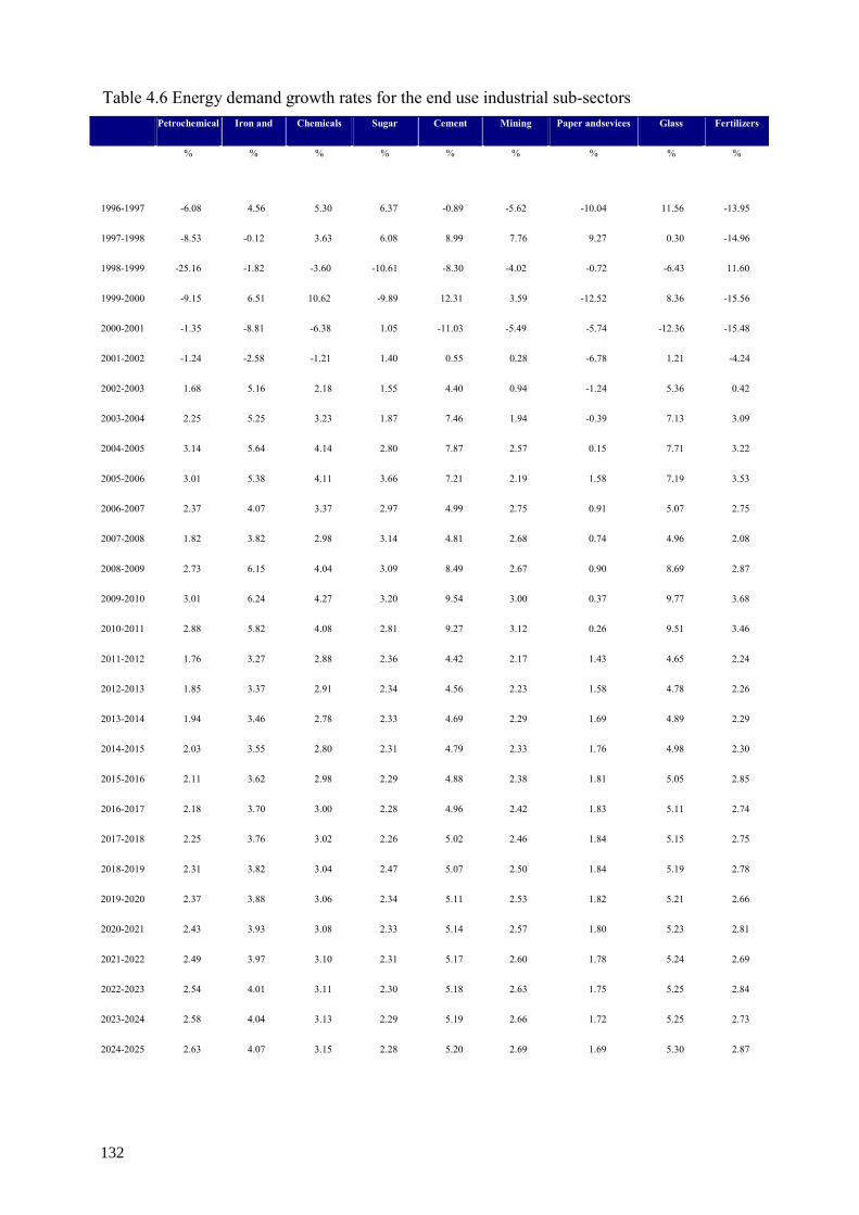
Table 4.6 Energy demand growth rates for the end use industrial sub-sectors Petrochemical Iron and Chemicals Sugar Cement Mining Paper andsevices Glass Fertilizers

% % % % % % % % %

1996-1997 -6.08 4.56 5.30 6.37 -0.89 -5.62 -10.04 11.56 -13.95

1997-1998 -8.53 -0.12 3.63 6.08 8.99 7.76 9.27 0.30 -14.96

1998-1999 -25.16 -1.82 -3.60 -10.61 -8.30 -4.02 -0.72 -6.43 11.60

1999-2000 -9.15 6.51 10.62 -9.89 12.31 3.59 -12.52 8.36 -15.56

2000-2001 -1.35 -8.81 -6.38 1.05 -11.03 -5.49 -5.74 -12.36 -15.48

2001-2002 -1.24 -2.58 -1.21 1.40 0.55 0.28 -6.78 1.21 -4.24

2002-2003 1.68 5.16 2.18 1.55 4.40 0.94 -1.24 5.36 0.42

2003-2004 2.25 5.25 3.23 1.87 7.46 1.94 -0.39 7.13 3.09

2004-2005 3.14 5.64 4.14 2.80 7.87 2.57 0.15 7.71 3.22

2005-2006 3.01 5.38 4.11 3.66 7.21 2.19 1.58 7.19 3.53

2006-2007 2.37 4.07 3.37 2.97 4.99 2.75 0.91 5.07 2.75

2007-2008 1.82 3.82 2.98 3.14 4.81 2.68 0.74 4.96 2.08

2008-2009 2.73 6.15 4.04 3.09 8.49 2.67 0.90 8.69 2.87

2009-2010 3.01 6.24 4.27 3.20 9.54 3.00 0.37 9.77 3.68

2010-2011 2.88 5.82 4.08 2.81 9.27 3.12 0.26 9.51 3.46

2011-2012 1.76 3.27 2.88 2.36 4.42 2.17 1.43 4.65 2.24

2012-2013 1.85 3.37 2.91 2.34 4.56 2.23 1.58 4.78 2.26

2013-2014 1.94 3.46 2.78 2.33 4.69 2.29 1.69 4.89 2.29

2014-2015 2.03 3.55 2.80 2.31 4.79 2.33 1.76 4.98 2.30

2015-2016 2.11 3.62 2.98 2.29 4.88 2.38 1.81 5.05 2.85

2016-2017 2.18 3.70 3.00 2.28 4.96 2.42 1.83 5.11 2.74

2017-2018 2.25 3.76 3.02 2.26 5.02 2.46 1.84 5.15 2.75

2018-2019 2.31 3.82 3.04 2.47 5.07 2.50 1.84 5.19 2.78

2019-2020 2.37 3.88 3.06 2.34 5.11 2.53 1.82 5.21 2.66

2020-2021 2.43 3.93 3.08 2.33 5.14 2.57 1.80 5.23 2.81

2021-2022 2.49 3.97 3.10 2.31 5.17 2.60 1.78 5.24 2.69

2022-2023 2.54 4.01 3.11 2.30 5.18 2.63 1.75 5.25 2.84

2023-2024 2.58 4.04 3.13 2.29 5.19 2.66 1.72 5.25 2.73

2024-2025 2.63 4.07 3.15 2.28 5.20 2.69 1.69 5.30 2.87

132

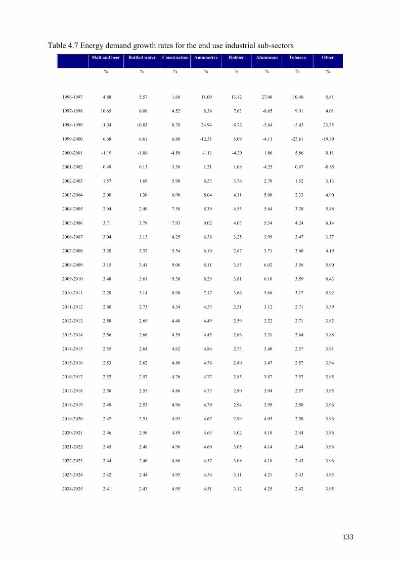
Table 4.7 Energy demand growth rates for the end use industrial sub-sectors Malt and beer Bottled water Construction Automotive Rubber Aluminum Tobacco Other

% % % % % % % %

1996-1997 4.88 5.57 1.60 11.00 13.12 27.40 10.40 5.81

1997-1998 10.65 6.08 4.52 8.36 7.63 -8.65 9.91 4.01

1998-1999 -1.34 10.83 8.78 24.94 -5.72 -5.64 -3.43 23.75

1999-2000 6.68 6.61 6.88 -12.31 5.09 -4.11 -23.61 -19.89

2000-2001 -1.19 -1.86 -4.50 -1.11 -4.29 1.86 5.86 0.11

2001-2002 0.49 0.13 3.30 1.21 1.08 -4.25 0.67 -0.85

2002-2003 1.57 1.69 5.90 6.53 3.76 2.70 1.52 3.13

2003-2004 2.00 1.30 6.98 8.04 4.11 5.00 2.33 4.90

2004-2005 2.94 2.49 7.58 8.39 4.55 5.64 3.28 5.48

2005-2006 3.71 3.78 7.93 9.02 4.03 5.34 4.24 6.14

2006-2007 3.04 3.13 4.25 6.38 3.25 3.99 3.47 3.77

2007-2008 3.20 3.37 5.54 6.10 2.67 3.71 3.60 4.19

2008-2009 3.15 3.41 9.06 8.11 3.55 6.02 3.56 5.90

2009-2010 3.48 3.61 9.38 8.29 3.81 6.10 3.59 6.43

2010-2011 2.28 3.14 8.90 7.17 3.66 5.68 3.17 5.92

2011-2012 2.60 2.73 4.34 4.53 2.51 3.12 2.71 3.59

2012-2013 2.58 2.69 4.48 4.49 2.59 3.22 2.71 3.82

2013-2014 2.56 2.66 4.59 4.45 2.66 3.31 2.64 3.88

2014-2015 2.55 2.64 4.62 4.84 2.73 3.40 2.57 3.91

2015-2016 2.53 2.62 4.86 4.76 2.80 3.47 2.57 3.94

2016-2017 2.52 2.57 4.76 4.77 2.85 3.87 2.57 3.95

2017-2018 2.50 2.55 4.86 4.73 2.90 3.94 2.57 3.95

2018-2019 2.49 2.53 4.96 4.70 2.94 3.99 2.50 3.96

2019-2020 2.47 2.51 4.93 4.67 2.99 4.05 2.50 3.96

2020-2021 2.46 2.50 4.89 4.63 3.02 4.10 2.44 3.96

2021-2022 2.45 2.48 4.96 4.60 3.05 4.14 2.44 3.96

2022-2023 2.44 2.46 4.86 4.57 3.08 4.18 2.43 3.96

2023-2024 2.42 2.44 4.95 4.54 3.11 4.21 2.43 3.95

2024-2025 2.41 2.43 4.95 4.51 3.12 4.25 2.42 3.95

133

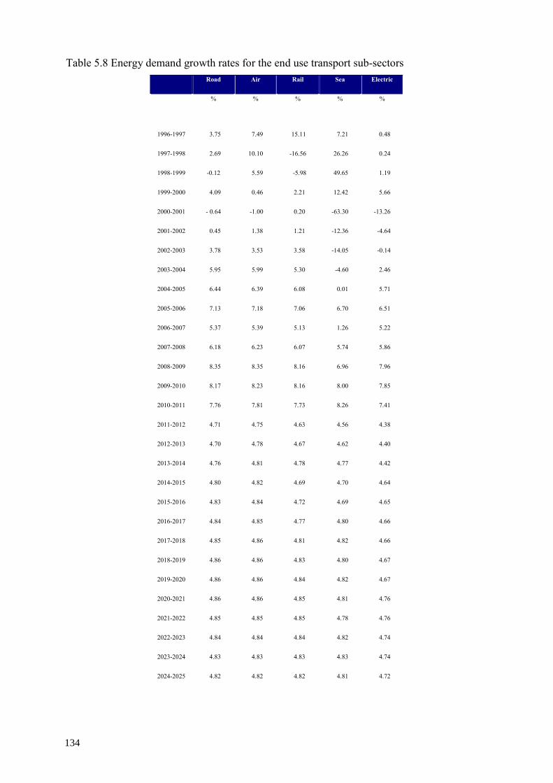
Table 5.8 Energy demand growth rates for the end use transport sub-sectors Road Air Rail Sea Electric

% % % % %

1996-1997 3.75 7.49 15.11 7.21 0.48

1997-1998 2.69 10.10 -16.56 26.26 0.24

1998-1999 -0.12 5.59 -5.98 49.65 1.19

1999-2000 4.09 0.46 2.21 12.42 5.66

2000-2001 - 0.64 -1.00 0.20 -63.30 -13.26

2001-2002 0.45 1.38 1.21 -12.36 -4.64

2002-2003 3.78 3.53 3.58 -14.05 -0.14

2003-2004 5.95 5.99 5.30 -4.60 2.46

2004-2005 6.44 6.39 6.08 0.01 5.71

2005-2006 7.13 7.18 7.06 6.70 6.51

2006-2007 5.37 5.39 5.13 1.26 5.22

2007-2008 6.18 6.23 6.07 5.74 5.86

2008-2009 8.35 8.35 8.16 6.96 7.96

2009-2010 8.17 8.23 8.16 8.00 7.85

2010-2011 7.76 7.81 7.73 8.26 7.41

2011-2012 4.71 4.75 4.63 4.56 4.38

2012-2013 4.70 4.78 4.67 4.62 4.40

2013-2014 4.76 4.81 4.78 4.77 4.42

2014-2015 4.80 4.82 4.69 4.70 4.64

2015-2016 4.83 4.84 4.72 4.69 4.65

2016-2017 4.84 4.85 4.77 4.80 4.66

2017-2018 4.85 4.86 4.81 4.82 4.66

2018-2019 4.86 4.86 4.83 4.80 4.67

2019-2020 4.86 4.86 4.84 4.82 4.67

2020-2021 4.86 4.86 4.85 4.81 4.76

2021-2022 4.85 4.85 4.85 4.78 4.76

2022-2023 4.84 4.84 4.84 4.82 4.74

2023-2024 4.83 4.83 4.83 4.83 4.74

2024-2025 4.82 4.82 4.82 4.81 4.72

134

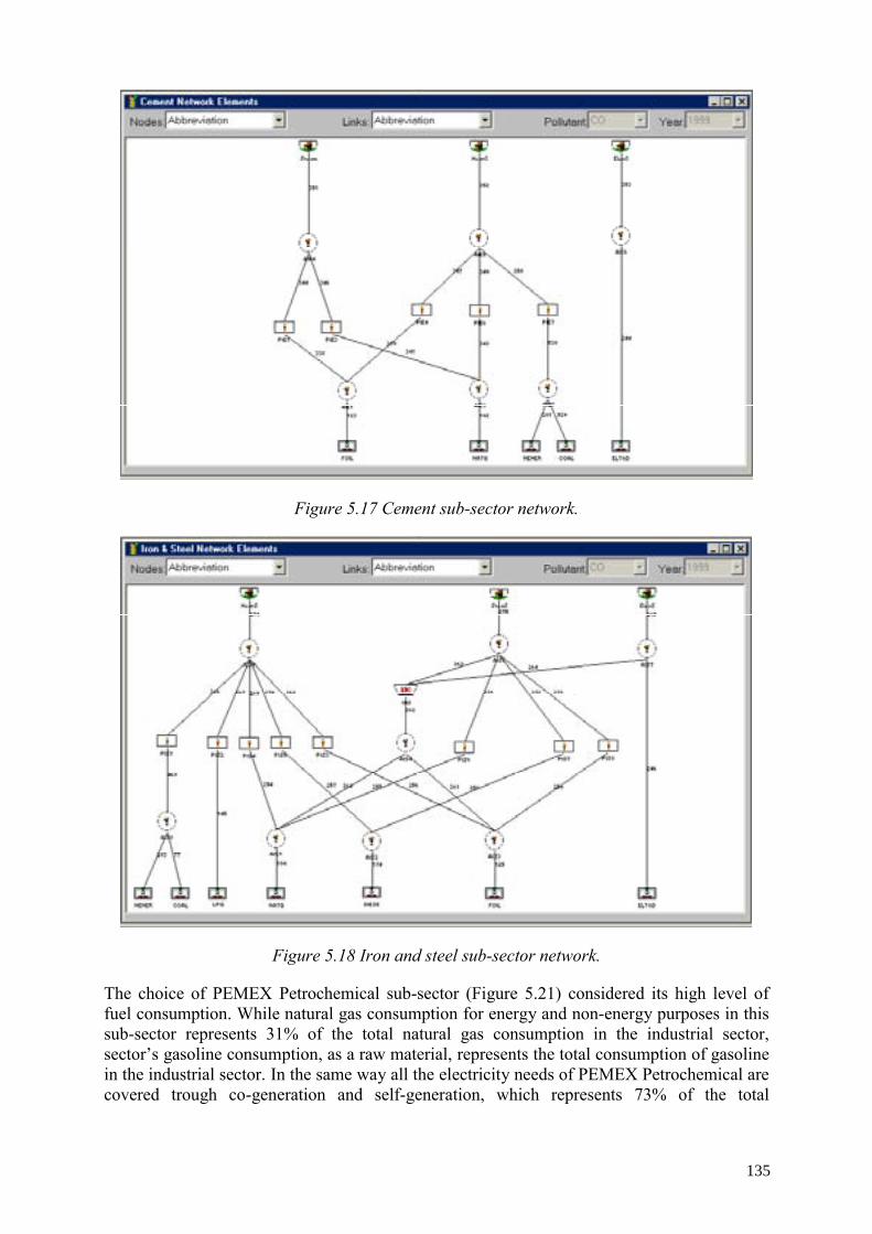
Figure 5.17 Cement sub-sector network.

Figure 5.18 Iron and steel sub-sector network.

The choice of PEMEX Petrochemical sub-sector (Figure 5.21) considered its high level of fuel consumption. While natural gas consumption for energy and non-energy purposes in this sub-sector represents 31% of the total natural gas consumption in the industrial sector, sector’s gasoline consumption, as a raw material, represents the total consumption of gasoline in the industrial sector. In the same way all the electricity needs of PEMEX Petrochemical are covered trough co-generation and self-generation, which represents 73% of the total

135

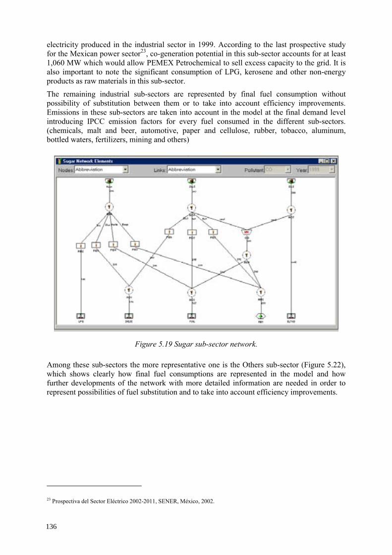
electricity produced in the industrial sector in 1999. According to the last prospective study for the Mexican power sector23, co-generation potential in this sub-sector accounts for at least 1,060 MW which would allow PEMEX Petrochemical to sell excess capacity to the grid. It is also important to note the significant consumption of LPG, kerosene and other non-energy products as raw materials in this sub-sector.

The remaining industrial sub-sectors are represented by final fuel consumption without possibility of substitution between them or to take into account efficiency improvements. Emissions in these sub-sectors are taken into account in the model at the final demand level introducing IPCC emission factors for every fuel consumed in the different sub-sectors. (chemicals, malt and beer, automotive, paper and cellulose, rubber, tobacco, aluminum, bottled waters, fertilizers, mining and others)

Figure 5.19 Sugar sub-sector network.

Among these sub-sectors the more representative one is the Others sub-sector (Figure 5.22), which shows clearly how final fuel consumptions are represented in the model and how further developments of the network with more detailed information are needed in order to represent possibilities of fuel substitution and to take into account efficiency improvements.

23 Prospectiva del Sector Eléctrico 2002-2011, SENER, México, 2002.

136

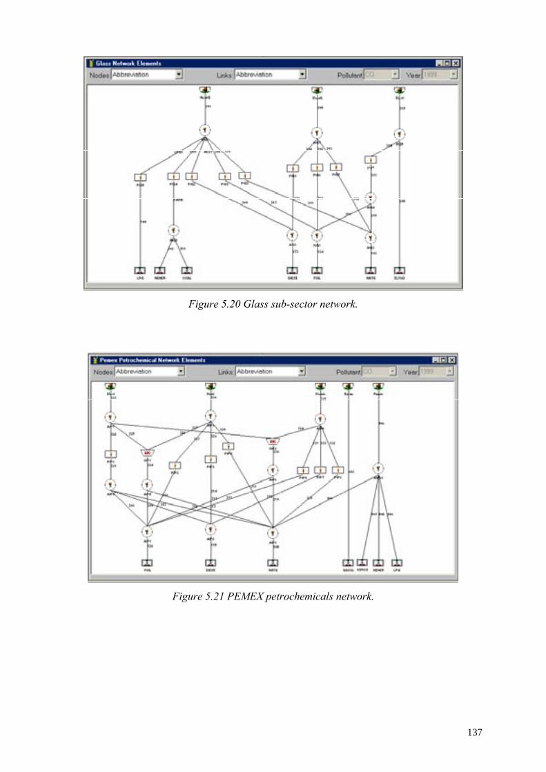
Figure 5.20 Glass sub-sector network.

Figure 5.21 PEMEX petrochemicals network.

137

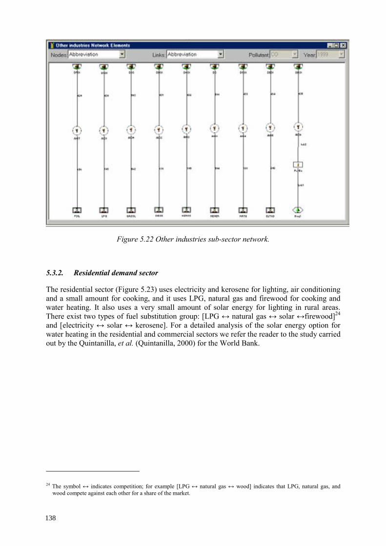
Figure 5.22 Other industries sub-sector network.

5.3.2. Residential demand sector

The residential sector (Figure 5.23) uses electricity and kerosene for lighting, air conditioning and a small amount for cooking, and it uses LPG, natural gas and firewood for cooking and water heating. It also uses a very small amount of solar energy for lighting in rural areas. There exist two types of fuel substitution group: [LPG ↔ natural gas ↔ solar ↔firewood]24 and [electricity ↔ solar ↔ kerosene]. For a detailed analysis of the solar energy option for water heating in the residential and commercial sectors we refer the reader to the study carried out by the Quintanilla, et al. (Quintanilla, 2000) for the World Bank.

24 The symbol ↔ indicates competition; for example [LPG ↔ natural gas ↔ wood] indicates that LPG, natural gas, and

wood compete against each other for a share of the market.

138

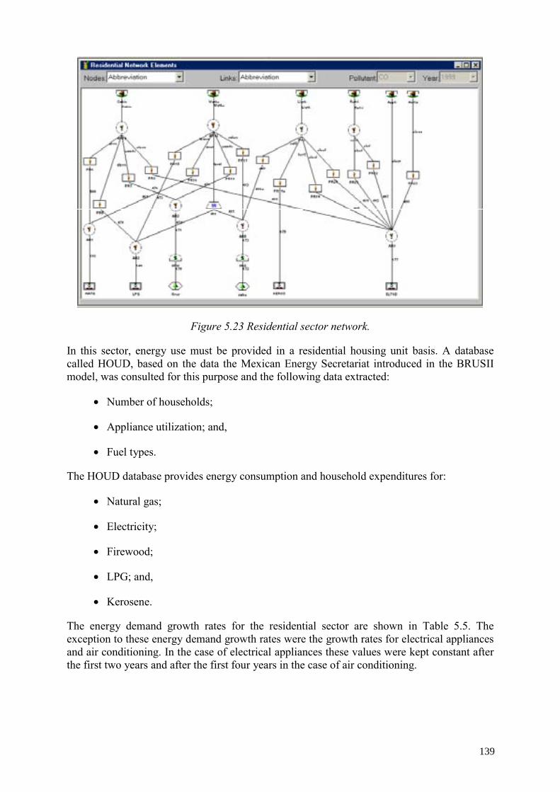
Figure 5.23 Residential sector network.

In this sector, energy use must be provided in a residential housing unit basis. A database called HOUD, based on the data the Mexican Energy Secretariat introduced in the BRUSII model, was consulted for this purpose and the following data extracted:

• Number of households;

• Appliance utilization; and,

• Fuel types.

The HOUD database provides energy consumption and household expenditures for:

• Natural gas;

• Electricity;

• Firewood;

• LPG; and,

• Kerosene.

The energy demand growth rates for the residential sector are shown in Table 5.5. The exception to these energy demand growth rates were the growth rates for electrical appliances and air conditioning. In the case of electrical appliances these values were kept constant after the first two years and after the first four years in the case of air conditioning.

139

5.3.3. Transport demand sector

For the transport sector (Figure 5.24), fuel demand was divided into the following categories: rail, sea, air, road and electric. Rail transport use diesel, sea and water transport can use fuel oil or diesel, air transport use jet fuel and kerosene. Road transport uses diesel, gasoline, LPG and natural gas. Transport sector constitutes the major energy-demanding sector in the Mexican energy system, it accounts for the 39% of total energy consumption.

Figure 5.24 Transport sector network.

The transportation sector is fundamentally different to other demand sectors since it represents as a part of service sector. Transportation is used to support other activities in the industrial, commercial and residential sector. Lack of official Mexican data has meant that other resources must be used. The TRAN database (MAR, 2001) was used with a splitting in terms of transport mode, average distance traveled, technology, passenger and freight, number of vehicles. Changes in energy consumption can occur due to efficiency, technological and economic reasons. Because of this, trend scenarios were considered in a business-as-usual fashion where no major differences with the past trends occur, i.e., energy demand growth rates for individual transport modes conduct to the same total demand growth rates provided by MODEMA. Hybrid transport alternative refers to the vehicles that use hydrogen and electricity. The electricity is generated by renewable energy sources such as solar and wind. There are two types of fuel substitution group in the rod transportation mode: [natural gas and hybrid ↔ gasoline]25 and [LPG ↔ diesel].

5.3.4. Commercial and public demand sector

The commercial and public sector network is shown in Figure 5.25. The fuel mix in the commercial sector has changed significantly over the 1989–1999 period. In 1989 fuel oil 25 The symbol ↔ indicates competition; for example [LPG ↔ natural gas ↔ wood] indicates that LPG, natural gas, and

wood compete against each other for a share of the market.

140

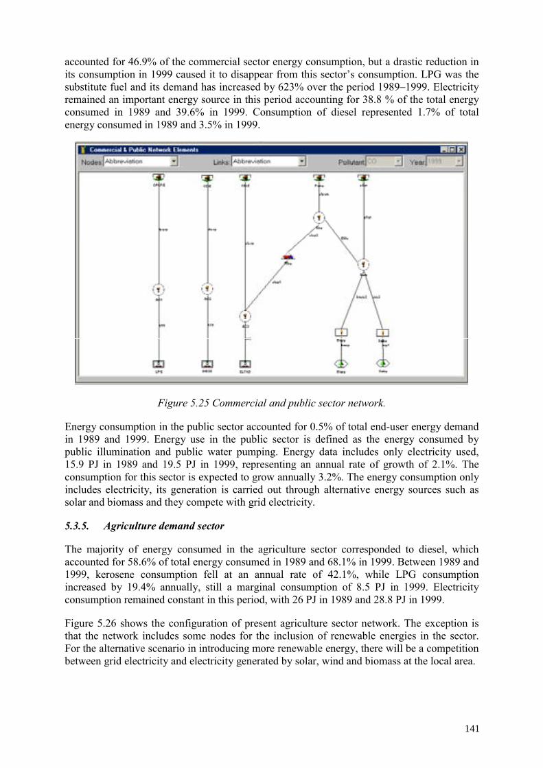
accounted for 46.9% of the commercial sector energy consumption, but a drastic reduction in its consumption in 1999 caused it to disappear from this sector’s consumption. LPG was the substitute fuel and its demand has increased by 623% over the period 1989–1999. Electricity remained an important energy source in this period accounting for 38.8 % of the total energy consumed in 1989 and 39.6% in 1999. Consumption of diesel represented 1.7% of total energy consumed in 1989 and 3.5% in 1999.

Figure 5.25 Commercial and public sector network.

Energy consumption in the public sector accounted for 0.5% of total end-user energy demand in 1989 and 1999. Energy use in the public sector is defined as the energy consumed by public illumination and public water pumping. Energy data includes only electricity used, 15.9 PJ in 1989 and 19.5 PJ in 1999, representing an annual rate of growth of 2.1%. The consumption for this sector is expected to grow annually 3.2%. The energy consumption only includes electricity, its generation is carried out through alternative energy sources such as solar and biomass and they compete with grid electricity.

5.3.5. Agriculture demand sector

The majority of energy consumed in the agriculture sector corresponded to diesel, which accounted for 58.6% of total energy consumed in 1989 and 68.1% in 1999. Between 1989 and 1999, kerosene consumption fell at an annual rate of 42.1%, while LPG consumption increased by 19.4% annually, still a marginal consumption of 8.5 PJ in 1999. Electricity consumption remained constant in this period, with 26 PJ in 1989 and 28.8 PJ in 1999.

Figure 5.26 shows the configuration of present agriculture sector network. The exception is that the network includes some nodes for the inclusion of renewable energies in the sector. For the alternative scenario in introducing more renewable energy, there will be a competition between grid electricity and electricity generated by solar, wind and biomass at the local area.

141

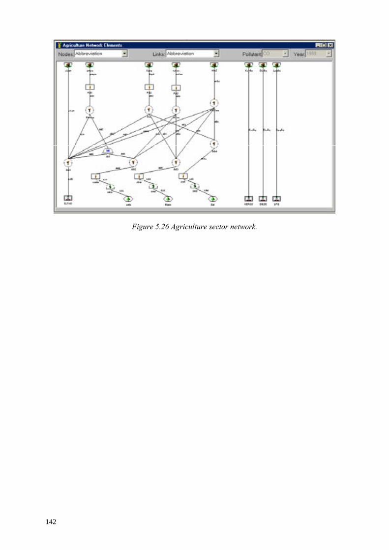
Figure 5.26 Agriculture sector network.

142

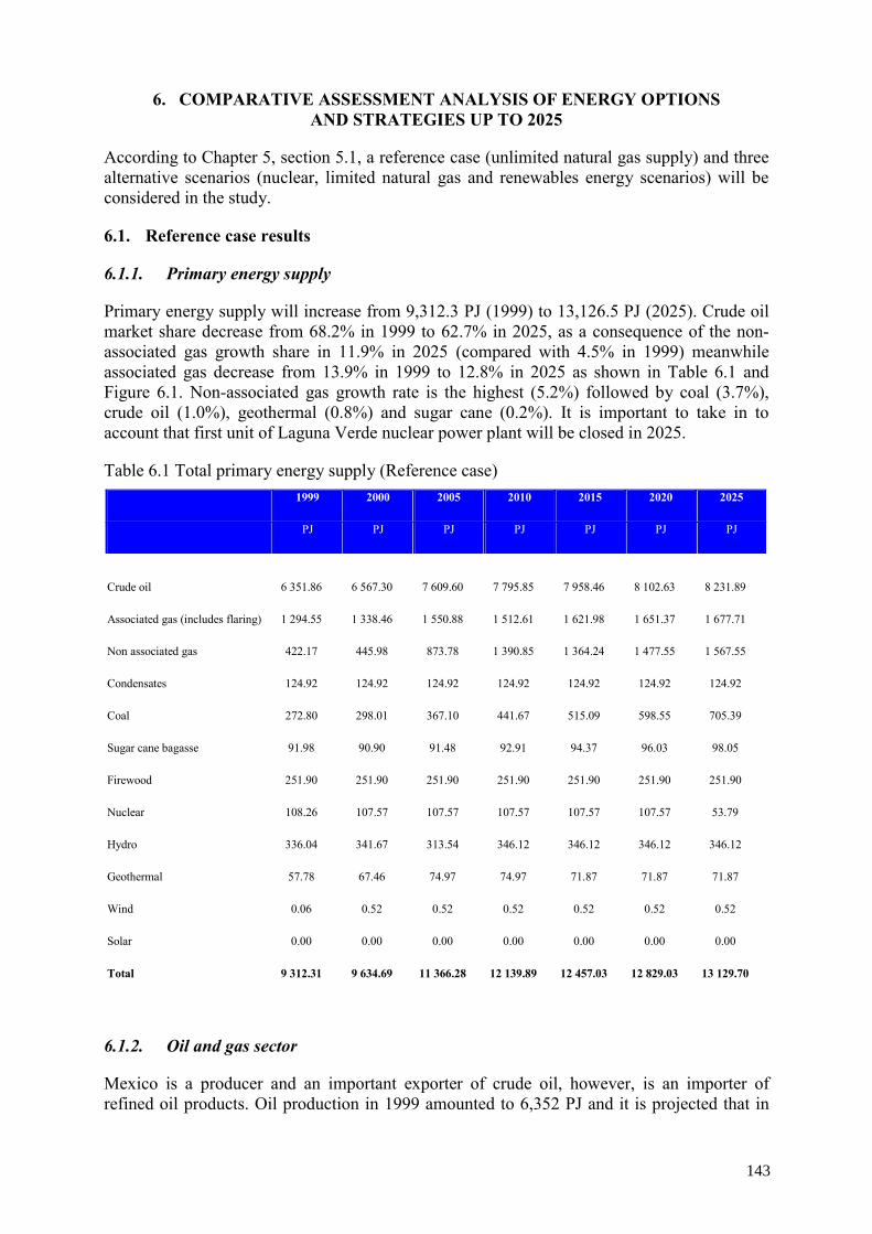
6. COMPARATIVE ASSESSMENT ANALYSIS OF ENERGY OPTIONS AND STRATEGIES UP TO 2025

According to Chapter 5, section 5.1, a reference case (unlimited natural gas supply) and three alternative scenarios (nuclear, limited natural gas and renewables energy scenarios) will be considered in the study.

6.1. Reference case results

6.1.1. Primary energy supply

Primary energy supply will increase from 9,312.3 PJ (1999) to 13,126.5 PJ (2025). Crude oil market share decrease from 68.2% in 1999 to 62.7% in 2025, as a consequence of the non-associated gas growth share in 11.9% in 2025 (compared with 4.5% in 1999) meanwhile associated gas decrease from 13.9% in 1999 to 12.8% in 2025 as shown in Table 6.1 and Figure 6.1. Non-associated gas growth rate is the highest (5.2%) followed by coal (3.7%), crude oil (1.0%), geothermal (0.8%) and sugar cane (0.2%). It is important to take in to account that first unit of Laguna Verde nuclear power plant will be closed in 2025.

Table 6.1 Total primary energy supply (Reference case) 1999 2000 2005 2010 2015 2020 2025

PJ PJ PJ PJ PJ PJ PJ

Crude oil 6 351.86 6 567.30 7 609.60 7 795.85 7 958.46 8 102.63 8 231.89

Associated gas (includes flaring) 1 294.55 1 338.46 1 550.88 1 512.61 1 621.98 1 651.37 1 677.71

Non associated gas 422.17 445.98 873.78 1 390.85 1 364.24 1 477.55 1 567.55

Condensates 124.92 124.92 124.92 124.92 124.92 124.92 124.92

Coal 272.80 298.01 367.10 441.67 515.09 598.55 705.39

Sugar cane bagasse 91.98 90.90 91.48 92.91 94.37 96.03 98.05

Firewood 251.90 251.90 251.90 251.90 251.90 251.90 251.90

Nuclear 108.26 107.57 107.57 107.57 107.57 107.57 53.79

Hydro 336.04 341.67 313.54 346.12 346.12 346.12 346.12

Geothermal 57.78 67.46 74.97 74.97 71.87 71.87 71.87

Wind 0.06 0.52 0.52 0.52 0.52 0.52 0.52

Solar 0.00 0.00 0.00 0.00 0.00 0.00 0.00

Total 9 312.31 9 634.69 11 366.28 12 139.89 12 457.03 12 829.03 13 129.70

6.1.2. Oil and gas sector

Mexico is a producer and an important exporter of crude oil, however, is an importer of refined oil products. Oil production in 1999 amounted to 6,352 PJ and it is projected that in

143

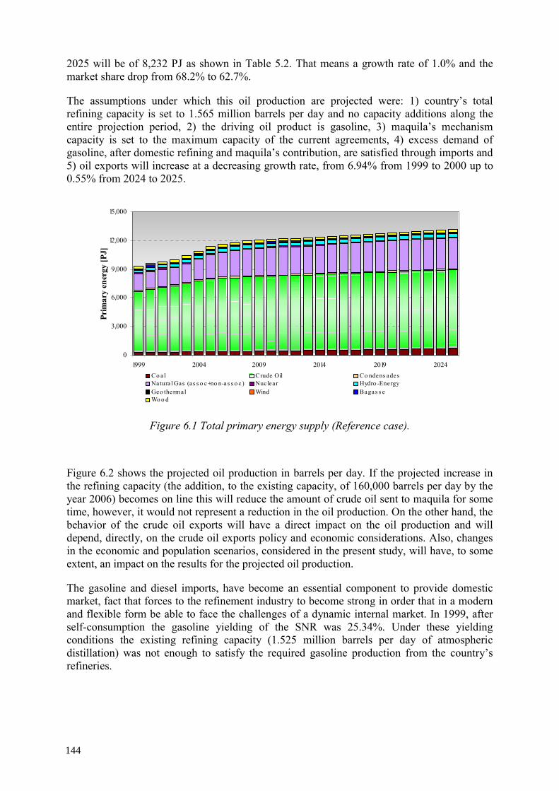
2025 will be of 8,232 PJ as shown in Table 5.2. That means a growth rate of 1.0% and the market share drop from 68.2% to 62.7%.

The assumptions under which this oil production are projected were: 1) country’s total refining capacity is set to 1.565 million barrels per day and no capacity additions along the entire projection period, 2) the driving oil product is gasoline, 3) maquila’s mechanism capacity is set to the maximum capacity of the current agreements, 4) excess demand of gasoline, after domestic refining and maquila’s contribution, are satisfied through imports and 5) oil exports will increase at a decreasing growth rate, from 6.94% from 1999 to 2000 up to 0.55% from 2024 to 2025.

0

3,000

6,000

9,000

12,000

15,000

1999 2004 2009 2014 2019 2024

Prim

ary

ener

gy [P

J]

Co al Crude Oil Co ndens adesNatura l Gas (as s o c+no n-a s s o c ) Nuclear Hydro -EnergyGeo thermal Wind Bagas s eWo o d

Figure 6.1 Total primary energy supply (Reference case).

Figure 6.2 shows the projected oil production in barrels per day. If the projected increase in the refining capacity (the addition, to the existing capacity, of 160,000 barrels per day by the year 2006) becomes on line this will reduce the amount of crude oil sent to maquila for some time, however, it would not represent a reduction in the oil production. On the other hand, the behavior of the crude oil exports will have a direct impact on the oil production and will depend, directly, on the crude oil exports policy and economic considerations. Also, changes in the economic and population scenarios, considered in the present study, will have, to some extent, an impact on the results for the projected oil production.

The gasoline and diesel imports, have become an essential component to provide domestic market, fact that forces to the refinement industry to become strong in order that in a modern and flexible form be able to face the challenges of a dynamic internal market. In 1999, after self-consumption the gasoline yielding of the SNR was 25.34%. Under these yielding conditions the existing refining capacity (1.525 million barrels per day of atmospheric distillation) was not enough to satisfy the required gasoline production from the country’s refineries.

144

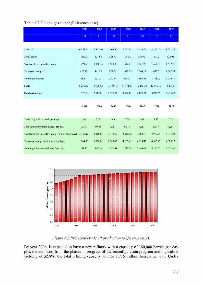
Table 6.2 Oil and gas sector (Reference case) 1999 2000 2005 2010 2015 2020 2025


Crude oil 6 351.86 6 567.30 7 609.60 7 795.85 7 958.46 8 102.63 8 231.89

Condensates 124.92 124.92 124.92 124.92 124.92 124.92 124.92

Associated gas (includes flaring) 1 294.55 1 338.46 1 550.88 1 512.61 1 621.98 1 651.37 1 677.71

Non-associated gas 422.17 445.98 873.78 1 390.85 1 364.24 1 477.55 1 567.55

Natural gas imports 59.87 231.38 550.54 620.67 1 193.52 1 808.65 2 689.81

Total 8 253.37 8 708.02 10 709.73 11 444.90 12 263.12 13 165.12 14 291.87

Total natural gas 1 776.59 2 015.81 2 975.21 3 524.13 4 179.74 4 937.57 5 935.07

1999 2000 2005 2010 2015 2020 2025

Crude oil (million barrels per day) 2.91 3.00 3.49 3.58 3.65 3.72 3.78

Condensates (thousand barrels per day) 93.48 93.48 92.87 92.87 92.87 92.87 92.87

Associated gas (includes flaring; million cf per day) 3 133.47 3 215.53 3 710.39 3 618.82 3 880.50 3 950.79 4 013.82

Non-associated gas (million cf per day) 1 264.90 1 334.83 2 580.45 4 107.45 4 028.85 4 363.49 4 629.27

Natural gas imports (million cf per day) 168.50 649.29 1 570.68 1 770.74 3 405.07 5 160.02 7 673.92

0.0

0.5

1.0

1.5

2.0

2.5

3.0

3.5

4.0

1999 2004 2009 2014 2019 2024

mill

ion

barr

els p

er d

ay

Figure 6.2 Projected crude oil production (Reference case).

By year 2006, is expected to have a new refinery with a capacity of 160,000 barrels per day plus the additions from the phases in progress of the reconfiguration program and a gasoline yielding of 32.8%, the total refining capacity will be 1.715 million barrels per day. Under

145

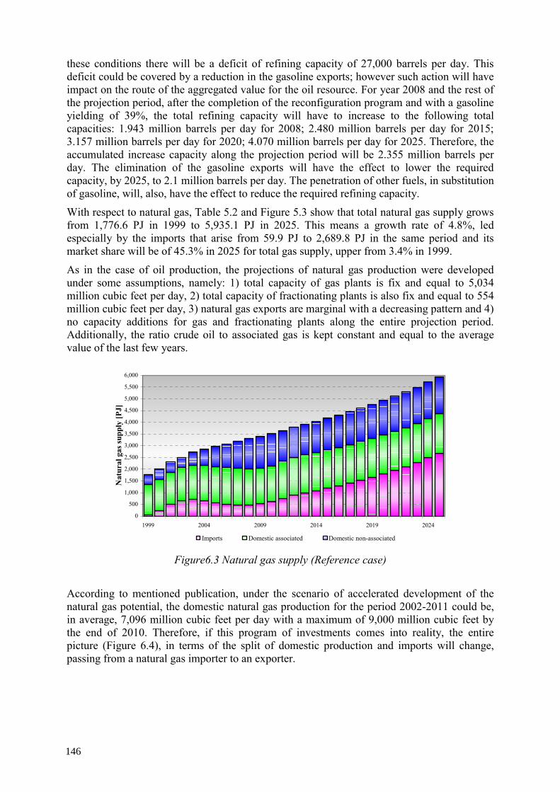
these conditions there will be a deficit of refining capacity of 27,000 barrels per day. This deficit could be covered by a reduction in the gasoline exports; however such action will have impact on the route of the aggregated value for the oil resource. For year 2008 and the rest of the projection period, after the completion of the reconfiguration program and with a gasoline yielding of 39%, the total refining capacity will have to increase to the following total capacities: 1.943 million barrels per day for 2008; 2.480 million barrels per day for 2015; 3.157 million barrels per day for 2020; 4.070 million barrels per day for 2025. Therefore, the accumulated increase capacity along the projection period will be 2.355 million barrels per day. The elimination of the gasoline exports will have the effect to lower the required capacity, by 2025, to 2.1 million barrels per day. The penetration of other fuels, in substitution of gasoline, will, also, have the effect to reduce the required refining capacity.

With respect to natural gas, Table 5.2 and Figure 5.3 show that total natural gas supply grows from 1,776.6 PJ in 1999 to 5,935.1 PJ in 2025. This means a growth rate of 4.8%, led especially by the imports that arise from 59.9 PJ to 2,689.8 PJ in the same period and its market share will be of 45.3% in 2025 for total gas supply, upper from 3.4% in 1999.

As in the case of oil production, the projections of natural gas production were developed under some assumptions, namely: 1) total capacity of gas plants is fix and equal to 5,034 million cubic feet per day, 2) total capacity of fractionating plants is also fix and equal to 554 million cubic feet per day, 3) natural gas exports are marginal with a decreasing pattern and 4) no capacity additions for gas and fractionating plants along the entire projection period. Additionally, the ratio crude oil to associated gas is kept constant and equal to the average value of the last few years.

0

500

1,000

1,500

2,000

2,500

3,000

3,500

4,000

4,500

5,000

5,500

6,000

1999 2004 2009 2014 2019 2024

Nat

ural

gas

supp

ly [P

J]

Imports Domestic associated Domestic non-associated Figure6.3 Natural gas supply (Reference case)

According to mentioned publication, under the scenario of accelerated development of the natural gas potential, the domestic natural gas production for the period 2002-2011 could be, in average, 7,096 million cubic feet per day with a maximum of 9,000 million cubic feet by the end of 2010. Therefore, if this program of investments comes into reality, the entire picture (Figure 6.4), in terms of the split of domestic production and imports will change, passing from a natural gas importer to an exporter.

146

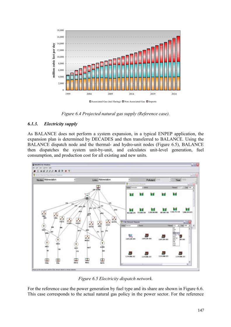
0

2,000

4,000

6,000

8,000

10,000

12,000

14,000

16,000

18,000

1999 2004 2009 2014 2019 2024

mill

ion

cubi

c fe

et p

er d

ay

Associated Gas (incl flaring) Non Associated Gas Imports

Figure 6.4 Projected natural gas supply (Reference case).

6.1.3. Electricity supply

As BALANCE does not perform a system expansion, in a typical ENPEP application, the expansion plan is determined by DECADES and then transferred to BALANCE. Using the BALANCE dispatch node and the thermal- and hydro-unit nodes (Figure 6.5), BALANCE then dispatches the system unit-by-unit, and calculates unit-level generation, fuel consumption, and production cost for all existing and new units.

Figure 6.5 Electricity dispatch network.

For the reference case the power generation by fuel type and its share are shown in Figure 6.6. This case corresponds to the actual natural gas policy in the power sector. For the reference

147

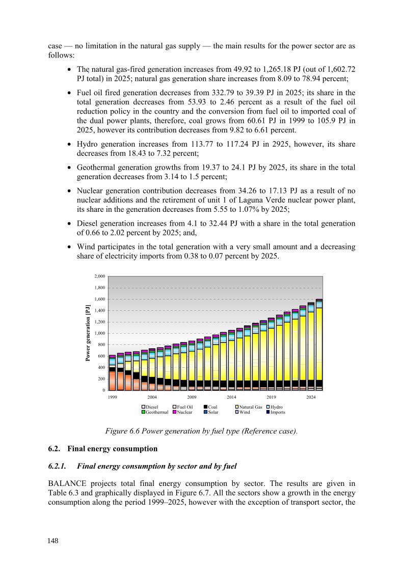
case — no limitation in the natural gas supply — the main results for the power sector are as follows:

• The natural gas-fired generation increases from 49.92 to 1,265.18 PJ (out of 1,602.72 PJ total) in 2025; natural gas generation share increases from 8.09 to 78.94 percent;

• Fuel oil fired generation decreases from 332.79 to 39.39 PJ in 2025; its share in the total generation decreases from 53.93 to 2.46 percent as a result of the fuel oil reduction policy in the country and the conversion from fuel oil to imported coal of the dual power plants, therefore, coal grows from 60.61 PJ in 1999 to 105.9 PJ in 2025, however its contribution decreases from 9.82 to 6.61 percent.

• Hydro generation increases from 113.77 to 117.24 PJ in 2925, however, its share decreases from 18.43 to 7.32 percent;

• Geothermal generation growths from 19.37 to 24.1 PJ by 2025, its share in the total generation decreases from 3.14 to 1.5 percent;

• Nuclear generation contribution decreases from 34.26 to 17.13 PJ as a result of no nuclear additions and the retirement of unit 1 of Laguna Verde nuclear power plant, its share in the generation decreases from 5.55 to 1.07% by 2025;

• Diesel generation increases from 4.1 to 32.44 PJ with a share in the total generation of 0.66 to 2.02 percent by 2025; and,

• Wind participates in the total generation with a very small amount and a decreasing share of electricity imports from 0.38 to 0.07 percent by 2025.

0

200

400

600

800

1,000

1,200

1,400

1,600

1,800

2,000

1999 2004 2009 2014 2019 2024

Pow

er g

ener

atio

n [P

J]

Diesel Fuel Oil Coal Natural Gas HydroGeothermal Nuclear Solar Wind Imports

Figure 6.6 Power generation by fuel type (Reference case).

6.2. Final energy consumption

6.2.1. Final energy consumption by sector and by fuel

BALANCE projects total final energy consumption by sector. The results are given in Table 6.3 and graphically displayed in Figure 6.7. All the sectors show a growth in the energy consumption along the period 1999–2025, however with the exception of transport sector, the

148

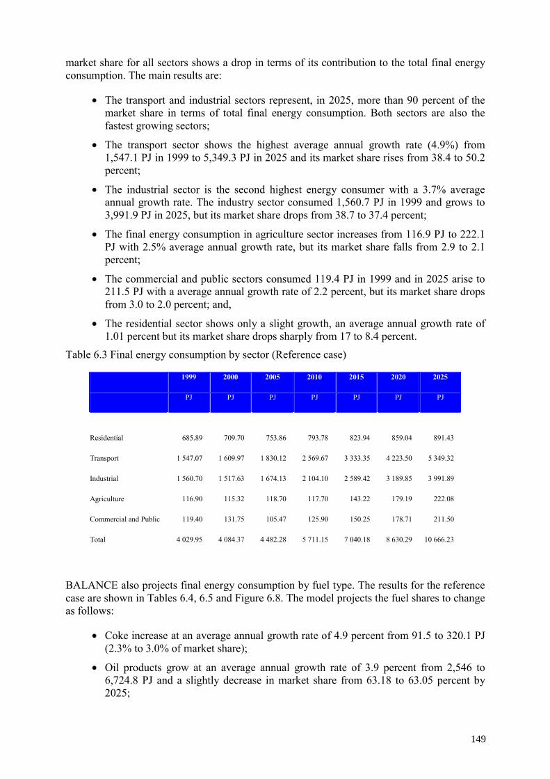
market share for all sectors shows a drop in terms of its contribution to the total final energy consumption. The main results are:

• The transport and industrial sectors represent, in 2025, more than 90 percent of the market share in terms of total final energy consumption. Both sectors are also the fastest growing sectors;

• The transport sector shows the highest average annual growth rate (4.9%) from 1,547.1 PJ in 1999 to 5,349.3 PJ in 2025 and its market share rises from 38.4 to 50.2 percent;

• The industrial sector is the second highest energy consumer with a 3.7% average annual growth rate. The industry sector consumed 1,560.7 PJ in 1999 and grows to 3,991.9 PJ in 2025, but its market share drops from 38.7 to 37.4 percent;

• The final energy consumption in agriculture sector increases from 116.9 PJ to 222.1 PJ with 2.5% average annual growth rate, but its market share falls from 2.9 to 2.1 percent;

• The commercial and public sectors consumed 119.4 PJ in 1999 and in 2025 arise to 211.5 PJ with a average annual growth rate of 2.2 percent, but its market share drops from 3.0 to 2.0 percent; and,

• The residential sector shows only a slight growth, an average annual growth rate of 1.01 percent but its market share drops sharply from 17 to 8.4 percent.

Table 6.3 Final energy consumption by sector (Reference case)

1999 2000 2005 2010 2015 2020 2025


Residential 685.89 709.70 753.86 793.78 823.94 859.04 891.43

Transport 1 547.07 1 609.97 1 830.12 2 569.67 3 333.35 4 223.50 5 349.32

Industrial 1 560.70 1 517.63 1 674.13 2 104.10 2 589.42 3 189.85 3 991.89

Agriculture 116.90 115.32 118.70 117.70 143.22 179.19 222.08

Commercial and Public 119.40 131.75 105.47 125.90 150.25 178.71 211.50

Total 4 029.95 4 084.37 4 482.28 5 711.15 7 040.18 8 630.29 10 666.23

BALANCE also projects final energy consumption by fuel type. The results for the reference case are shown in Tables 6.4, 6.5 and Figure 6.8. The model projects the fuel shares to change as follows:

• Coke increase at an average annual growth rate of 4.9 percent from 91.5 to 320.1 PJ (2.3% to 3.0% of market share);

• Oil products grow at an average annual growth rate of 3.9 percent from 2,546 to 6,724.8 PJ and a slightly decrease in market share from 63.18 to 63.05 percent by 2025;

149

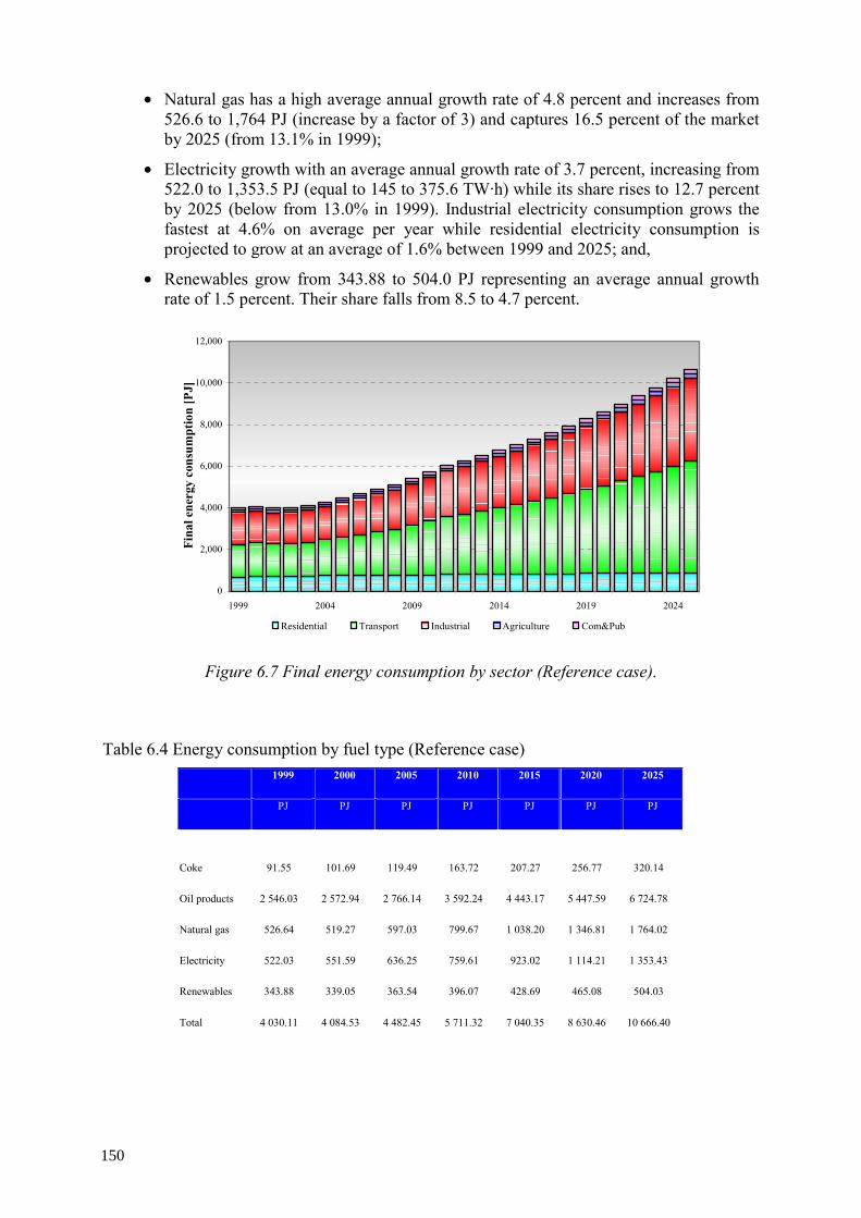
• Natural gas has a high average annual growth rate of 4.8 percent and increases from 526.6 to 1,764 PJ (increase by a factor of 3) and captures 16.5 percent of the market by 2025 (from 13.1% in 1999);

• Electricity growth with an average annual growth rate of 3.7 percent, increasing from 522.0 to 1,353.5 PJ (equal to 145 to 375.6 TW·h) while its share rises to 12.7 percent by 2025 (below from 13.0% in 1999). Industrial electricity consumption grows the fastest at 4.6% on average per year while residential electricity consumption is projected to grow at an average of 1.6% between 1999 and 2025; and,

• Renewables grow from 343.88 to 504.0 PJ representing an average annual growth rate of 1.5 percent. Their share falls from 8.5 to 4.7 percent.

0

2,000

4,000

6,000

8,000

10,000

12,000

1999 2004 2009 2014 2019 2024

Fina

l ene

rgy

cons

umpt

ion

[PJ]

Residential Transport Industrial Agriculture Com&Pub

Figure 6.7 Final energy consumption by sector (Reference case).

Table 6.4 Energy consumption by fuel type (Reference case) 1999 2000 2005 2010 2015 2020 2025


Coke 91.55 101.69 119.49 163.72 207.27 256.77 320.14

Oil products 2 546.03 2 572.94 2 766.14 3 592.24 4 443.17 5 447.59 6 724.78

Natural gas 526.64 519.27 597.03 799.67 1 038.20 1 346.81 1 764.02

Electricity 522.03 551.59 636.25 759.61 923.02 1 114.21 1 353.43

Renewables 343.88 339.05 363.54 396.07 428.69 465.08 504.03

Total 4 030.11 4 084.53 4 482.45 5 711.32 7 040.35 8 630.46 10 666.40

150

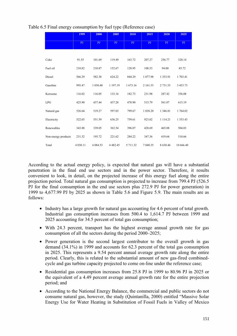
Table 6.5 Final energy consumption by fuel type (Reference case) 1999 2000 2005 2010 2015 2020 2025


Coke 91.55 101.69 119.49 163.72 207.27 256.77 320.14

Fuel oil 210.82 210.87 152.67 128.95 108.53 94.00 85.72

Diesel 566.29 582.38 624.22 844.29 1 077.98 1 353.91 1 703.41

Gasoline 995.47 1 030.48 1 197.19 1 673.16 2 161.53 2 731.55 3 453.73

Kerosene 116.02 116.05 133.16 182.73 231.98 287.42 356.08

LPG 425.90 437.44 437.28 478.90 515.79 561.07 615.19

Natural gas 526.64 519.27 597.03 799.67 1 038.20 1 346.81 1 764.02

Electricity 522.03 551.59 636.25 759.61 923.02 1 114.21 1 353.43

Renewables 343.88 339.05 363.54 396.07 428.69 465.08 504.03

Non-energy products 231.52 195.72 221.62 284.22 347.36 419.64 510.66

Total 4 030.11 4 084.53 4 482.45 5 711.32 7 040.35 8 630.46 10 666.40

According to the actual energy policy, is expected that natural gas will have a substantial penetration in the final end use sectors and in the power sector. Therefore, it results convenient to look, in detail, on the projected increase of this energy fuel along the entire projection period. Total natural gas consumption is projected to increase from 799.4 PJ (526.5 PJ for the final consumption in the end use sectors plus 272.9 PJ for power generation) in 1999 to 4,677.99 PJ by 2025 as shown in Table 5.6 and Figure 5.9. The main results are as follows:

• Industry has a large growth for natural gas accounting for 4.6 percent of total growth. Industrial gas consumption increases from 500.4 to 1,614.7 PJ between 1999 and 2025 accounting for 34.5 percent of total gas consumption;

• With 24.3 percent, transport has the highest average annual growth rate for gas consumption of all the sectors during the period 2000–2025;

• Power generation is the second largest contributor to the overall growth in gas demand (34.1%) in 1999 and accounts for 62.3 percent of the total gas consumption in 2025. This represents a 9.54 percent annual average growth rate along the entire period. Clearly, this is related to the substantial amount of new gas-fired combined-cycle and gas turbine capacity projected to come on-line under the reference case;

• Residential gas consumption increases from 25.8 PJ in 1999 to 80.96 PJ in 2025 or the equivalent of a 4.49 percent average annual growth rate for the entire projection period; and

• According to the National Energy Balance, the commercial and public sectors do not consume natural gas, however, the study (Quintanilla, 2000) entitled “Massive Solar Energy Use for Water Heating in Substitution of Fossil Fuels in Valley of Mexico

151

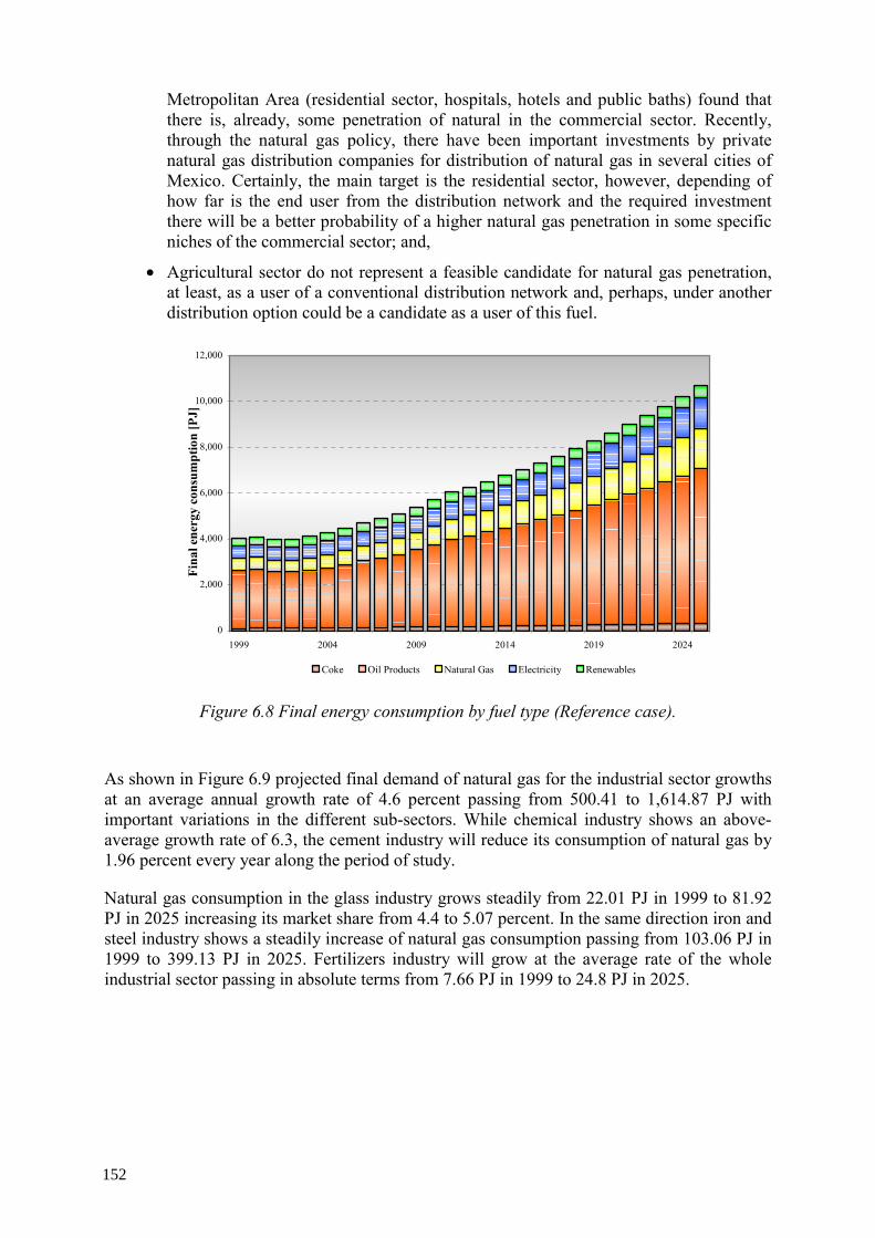
Metropolitan Area (residential sector, hospitals, hotels and public baths) found that there is, already, some penetration of natural in the commercial sector. Recently, through the natural gas policy, there have been important investments by private natural gas distribution companies for distribution of natural gas in several cities of Mexico. Certainly, the main target is the residential sector, however, depending of how far is the end user from the distribution network and the required investment there will be a better probability of a higher natural gas penetration in some specific niches of the commercial sector; and,

• Agricultural sector do not represent a feasible candidate for natural gas penetration, at least, as a user of a conventional distribution network and, perhaps, under another distribution option could be a candidate as a user of this fuel.

0

2,000

4,000

6,000

8,000

10,000

12,000

1999 2004 2009 2014 2019 2024

Fina

l ene

rgy

cons

umpt

ion

[PJ]

Coke Oil Products Natural Gas Electricity Renewables

Figure 6.8 Final energy consumption by fuel type (Reference case).

As shown in Figure 6.9 projected final demand of natural gas for the industrial sector growths at an average annual growth rate of 4.6 percent passing from 500.41 to 1,614.87 PJ with important variations in the different sub-sectors. While chemical industry shows an above-average growth rate of 6.3, the cement industry will reduce its consumption of natural gas by 1.96 percent every year along the period of study.

Natural gas consumption in the glass industry grows steadily from 22.01 PJ in 1999 to 81.92 PJ in 2025 increasing its market share from 4.4 to 5.07 percent. In the same direction iron and steel industry shows a steadily increase of natural gas consumption passing from 103.06 PJ in 1999 to 399.13 PJ in 2025. Fertilizers industry will grow at the average rate of the whole industrial sector passing in absolute terms from 7.66 PJ in 1999 to 24.8 PJ in 2025.

152

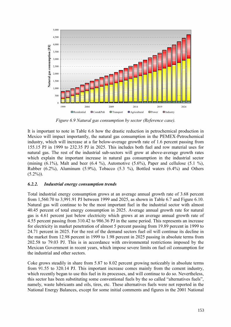
0

500

1,000

1,500

2,000

2,500

3,000

3,500

4,000

4,500

5,000

1999 2004 2009 2014 2019 2024

Nat

ural

gas

con

sum

ptio

n [P

J]

Residential Com&Pub Transport Agricultural Power Industry Figure 6.9 Natural gas consumption by sector (Reference case).

It is important to note in Table 6.6 how the drastic reduction in petrochemical production in Mexico will impact importantly, the natural gas consumption in the PEMEX-Petrochemical industry, which will increase at a far below-average growth rate of 1.6 percent passing from 155.15 PJ in 1999 to 232.35 PJ in 2025. This includes both fuel and row material uses for natural gas. The rest of the industrial sub-sectors will grow at above-average growth rates which explain the important increase in natural gas consumption in the industrial sector (mining (6.1%), Malt and beer (6.4 %), Automotive (5.6%), Paper and cellulose (5.1 %), Rubber (6.2%), Aluminum (5.9%), Tobacco (5.3 %), Bottled waters (6.4%) and Others (5.2%)).

6.2.2. Industrial energy consumption trends

Total industrial energy consumption grows at an average annual growth rate of 3.68 percent from 1,560.70 to 3,991.91 PJ between 1999 and 2025, as shown in Table 6.7 and Figure 6.10. Natural gas will continue to be the most important fuel in the industrial sector with almost 40.45 percent of total energy consumption in 2025. Average annual growth rate for natural gas is 4.61 percent just below electricity which grows at an average annual growth rate of 4.55 percent passing from 310.42 to 986.36 PJ in the same period. This represents an increase for electricity in market penetration of almost 5 percent passing from 19.89 percent in 1999 to 24.71 percent in 2025. For the rest of the demand sectors fuel oil will continue its decline in the market from 12.98 percent in 1999 to 1.98 percent in 2025 passing in absolute terms from 202.58 to 79.03 PJ. This is in accordance with environmental restrictions imposed by the Mexican Government in recent years, which impose severe limits on fuel oil consumption for the industrial and other sectors.

Coke grows steadily in share from 5.87 to 8.02 percent growing noticeably in absolute terms from 91.55 to 320.14 PJ. This important increase comes mainly from the cement industry, which recently began to use this fuel in its processes, and will continue to do so. Nevertheless, this sector has been substituting some conventional fuels by the so called “alternatives fuels”, namely, waste lubricants and oils, tires, etc. These alternatives fuels were not reported in the National Energy Balances, except for some initial comments and figures in the 2001 National

153

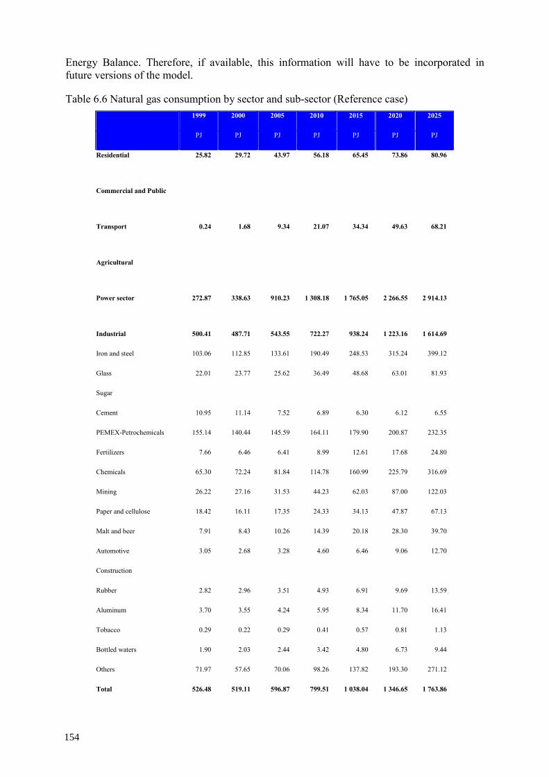
Energy Balance. Therefore, if available, this information will have to be incorporated in future versions of the model.

Table 6.6 Natural gas consumption by sector and sub-sector (Reference case) 1999 2000 2005 2010 2015 2020 2025


Residential 25.82 29.72 43.97 56.18 65.45 73.86 80.96

Commercial and Public

Transport 0.24 1.68 9.34 21.07 34.34 49.63 68.21

Agricultural

Power sector 272.87 338.63 910.23 1 308.18 1 765.05 2 266.55 2 914.13

Industrial 500.41 487.71 543.55 722.27 938.24 1 223.16 1 614.69

Iron and steel 103.06 112.85 133.61 190.49 248.53 315.24 399.12

Glass 22.01 23.77 25.62 36.49 48.68 63.01 81.93

Sugar

Cement 10.95 11.14 7.52 6.89 6.30 6.12 6.55

PEMEX-Petrochemicals 155.14 140.44 145.59 164.11 179.90 200.87 232.35

Fertilizers 7.66 6.46 6.41 8.99 12.61 17.68 24.80

Chemicals 65.30 72.24 81.84 114.78 160.99 225.79 316.69

Mining 26.22 27.16 31.53 44.23 62.03 87.00 122.03

Paper and cellulose 18.42 16.11 17.35 24.33 34.13 47.87 67.13

Malt and beer 7.91 8.43 10.26 14.39 20.18 28.30 39.70

Automotive 3.05 2.68 3.28 4.60 6.46 9.06 12.70

Construction

Rubber 2.82 2.96 3.51 4.93 6.91 9.69 13.59

Aluminum 3.70 3.55 4.24 5.95 8.34 11.70 16.41

Tobacco 0.29 0.22 0.29 0.41 0.57 0.81 1.13

Bottled waters 1.90 2.03 2.44 3.42 4.80 6.73 9.44

Others 71.97 57.65 70.06 98.26 137.82 193.30 271.12

Total 526.48 519.11 596.87 799.51 1 038.04 1 346.65 1 763.86

154

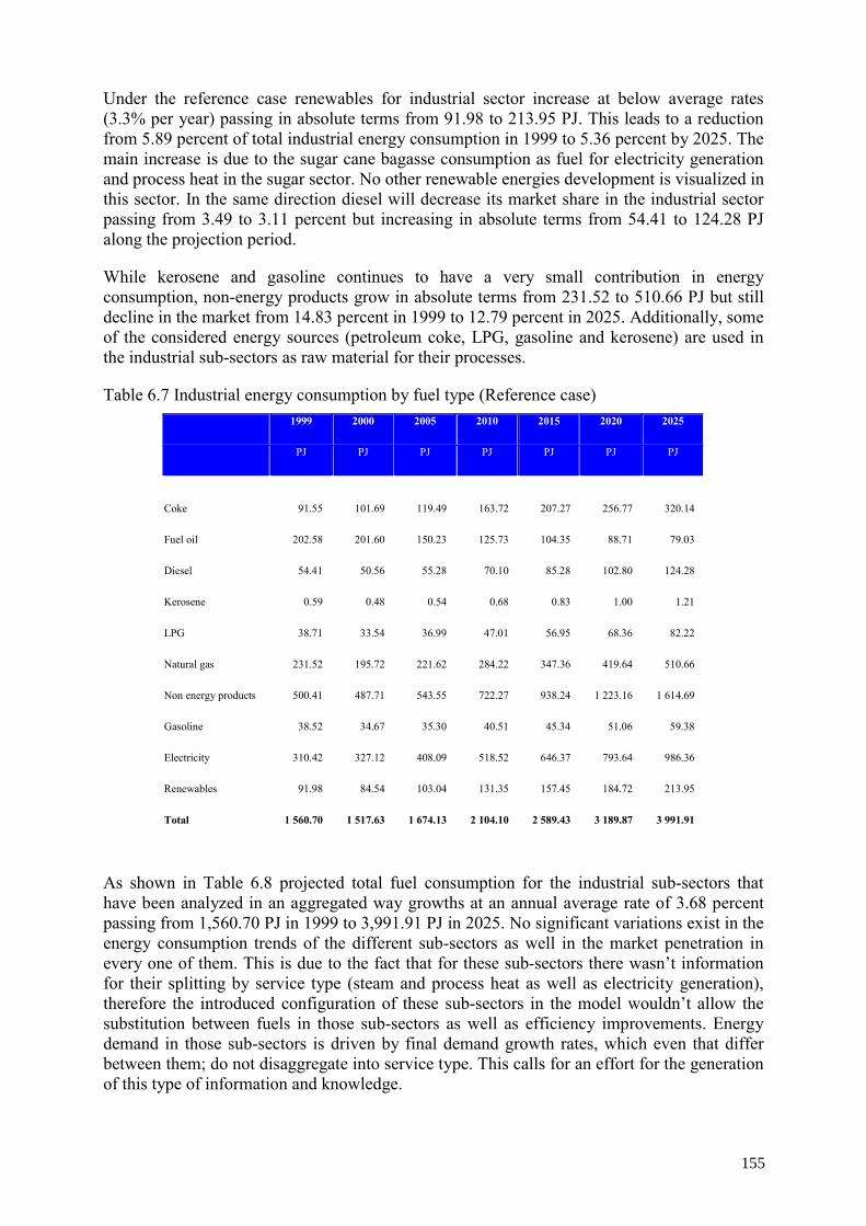
Under the reference case renewables for industrial sector increase at below average rates (3.3% per year) passing in absolute terms from 91.98 to 213.95 PJ. This leads to a reduction from 5.89 percent of total industrial energy consumption in 1999 to 5.36 percent by 2025. The main increase is due to the sugar cane bagasse consumption as fuel for electricity generation and process heat in the sugar sector. No other renewable energies development is visualized in this sector. In the same direction diesel will decrease its market share in the industrial sector passing from 3.49 to 3.11 percent but increasing in absolute terms from 54.41 to 124.28 PJ along the projection period.

While kerosene and gasoline continues to have a very small contribution in energy consumption, non-energy products grow in absolute terms from 231.52 to 510.66 PJ but still decline in the market from 14.83 percent in 1999 to 12.79 percent in 2025. Additionally, some of the considered energy sources (petroleum coke, LPG, gasoline and kerosene) are used in the industrial sub-sectors as raw material for their processes.

Table 6.7 Industrial energy consumption by fuel type (Reference case) 1999 2000 2005 2010 2015 2020 2025


Coke 91.55 101.69 119.49 163.72 207.27 256.77 320.14

Fuel oil 202.58 201.60 150.23 125.73 104.35 88.71 79.03

Diesel 54.41 50.56 55.28 70.10 85.28 102.80 124.28

Kerosene 0.59 0.48 0.54 0.68 0.83 1.00 1.21

LPG 38.71 33.54 36.99 47.01 56.95 68.36 82.22

Natural gas 231.52 195.72 221.62 284.22 347.36 419.64 510.66

Non energy products 500.41 487.71 543.55 722.27 938.24 1 223.16 1 614.69

Gasoline 38.52 34.67 35.30 40.51 45.34 51.06 59.38

Electricity 310.42 327.12 408.09 518.52 646.37 793.64 986.36

Renewables 91.98 84.54 103.04 131.35 157.45 184.72 213.95

Total 1 560.70 1 517.63 1 674.13 2 104.10 2 589.43 3 189.87 3 991.91

As shown in Table 6.8 projected total fuel consumption for the industrial sub-sectors that have been analyzed in an aggregated way growths at an annual average rate of 3.68 percent passing from 1,560.70 PJ in 1999 to 3,991.91 PJ in 2025. No significant variations exist in the energy consumption trends of the different sub-sectors as well in the market penetration in every one of them. This is due to the fact that for these sub-sectors there wasn’t information for their splitting by service type (steam and process heat as well as electricity generation), therefore the introduced configuration of these sub-sectors in the model wouldn’t allow the substitution between fuels in those sub-sectors as well as efficiency improvements. Energy demand in those sub-sectors is driven by final demand growth rates, which even that differ between them; do not disaggregate into service type. This calls for an effort for the generation of this type of information and knowledge.

155

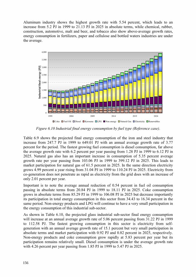
Aluminum industry shows the highest growth rate with 5.54 percent, which leads to an increase from 5.2 PJ in 1999 to 21.13 PJ in 2025 in absolute terms, while chemical, rubber, construction, automotive, malt and beer, and tobacco also show above-average growth rates, energy consumption in fertilizers, paper and cellulose and bottled waters industries are under the average.

0

500

1,000

1,500

2,000

2,500

3,000

3,500

4,000

1999 2004 2009 2014 2019 2024

Indu

stri

al fi

nal e

nerg

y [P

J]

Coke Fuel Oil Diesel Kerosene LPG Non energy Natural Gas Electricity Renewables

Figure 6.10 Industrial final energy consumption by fuel type (Reference case).

Table 6.9 shows the projected final energy consumption of the iron and steel industry that increase from 247.7 PJ in 1999 to 649.01 PJ with an annual average growth rate of 3.77 percent for the period. The fastest growing fuel consumption is diesel consumption, far above the average growth rate with 6.2 percent per year passing from 1.28 PJ in 1999 to 6.12 PJ in 2025. Natural gas also has an important increase in consumption of 5.35 percent average growth rate per year passing from 103.06 PJ in 1999 to 399.12 PJ in 2025. This leads to market participation for natural gas of 61.5 percent in 2025. In the same direction electricity grows 4.99 percent a year rising from 31.04 PJ in 1999 to 110.24 PJ in 2025. Electricity from co-generation does not penetrate as rapid as electricity from the grid does with an increase of only 2.01 percent per year.

Important is to note the average annual reduction of 0.54 percent in fuel oil consumption passing in absolute terms from 20.84 PJ in 1999 to 18.11 PJ in 2025. Coke consumption grows in absolute terms from 85.29 PJ in 1999 to 106.08 PJ in 2025 but decrease importantly its participation in total energy consumption in this sector from 34.43 to 16.34 percent in the same period. Non-energy products and LPG will continue to have a very small participation in the energy consumption of this industrial sub-sector.

As shown in Table 6.10, the projected glass industrial sub-sector final energy consumption will increase at an annual average growth rate of 5.06 percent passing from 31.22 PJ in 1999 to 112.58 PJ. The fastest growing consumption in this sector is electricity from self-generation with an annual average growth rate of 15.1 percent but very small participation in absolute terms and market participation with 0.92 PJ and 0.82 percent in 2025, respectively. Non-energy products and coke consumption grow rapidly at 5.83 percent per year but its participation remains relatively small. Diesel consumption is under the average growth rate with 4.26 percent per year passing from 1.85 PJ in 1999 to 5.47 PJ in 2025.

156

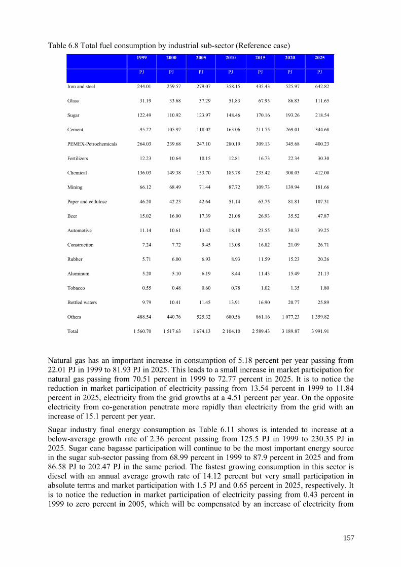
Table 6.8 Total fuel consumption by industrial sub-sector (Reference case) 1999 2000 2005 2010 2015 2020 2025


Iron and steel 244.01 259.57 279.07 358.15 435.43 525.97 642.82

Glass 31.19 33.68 37.29 51.83 67.95 86.83 111.65

Sugar 122.49 110.92 123.97 148.46 170.16 193.26 218.54

Cement 95.22 105.97 118.02 163.06 211.75 269.01 344.68

PEMEX-Petrochemicals 264.03 239.68 247.10 280.19 309.13 345.68 400.23

Fertilizers 12.23 10.64 10.15 12.81 16.73 22.34 30.30

Chemical 136.03 149.38 153.70 185.78 235.42 308.03 412.00

Mining 66.12 68.49 71.44 87.72 109.73 139.94 181.66

Paper and cellulose 46.20 42.23 42.64 51.14 63.75 81.81 107.31

Beer 15.02 16.00 17.39 21.08 26.93 35.52 47.87

Automotive 11.14 10.61 13.42 18.18 23.55 30.33 39.25

Construction 7.24 7.72 9.45 13.08 16.82 21.09 26.71

Rubber 5.71 6.00 6.93 8.93 11.59 15.23 20.26

Aluminum 5.20 5.10 6.19 8.44 11.43 15.49 21.13

Tobacco 0.55 0.48 0.60 0.78 1.02 1.35 1.80

Bottled waters 9.79 10.41 11.45 13.91 16.90 20.77 25.89

Others 488.54 440.76 525.32 680.56 861.16 1 077.23 1 359.82

Total 1 560.70 1 517.63 1 674.13 2 104.10 2 589.43 3 189.87 3 991.91

Natural gas has an important increase in consumption of 5.18 percent per year passing from 22.01 PJ in 1999 to 81.93 PJ in 2025. This leads to a small increase in market participation for natural gas passing from 70.51 percent in 1999 to 72.77 percent in 2025. It is to notice the reduction in market participation of electricity passing from 13.54 percent in 1999 to 11.84 percent in 2025, electricity from the grid growths at a 4.51 percent per year. On the opposite electricity from co-generation penetrate more rapidly than electricity from the grid with an increase of 15.1 percent per year.

Sugar industry final energy consumption as Table 6.11 shows is intended to increase at a below-average growth rate of 2.36 percent passing from 125.5 PJ in 1999 to 230.35 PJ in 2025. Sugar cane bagasse participation will continue to be the most important energy source in the sugar sub-sector passing from 68.99 percent in 1999 to 87.9 percent in 2025 and from 86.58 PJ to 202.47 PJ in the same period. The fastest growing consumption in this sector is diesel with an annual average growth rate of 14.12 percent but very small participation in absolute terms and market participation with 1.5 PJ and 0.65 percent in 2025, respectively. It is to notice the reduction in market participation of electricity passing from 0.43 percent in 1999 to zero percent in 2005, which will be compensated by an increase of electricity from

157

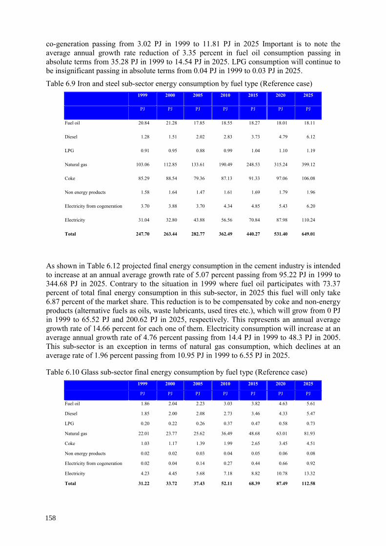
co-generation passing from 3.02 PJ in 1999 to 11.81 PJ in 2025 Important is to note the average annual growth rate reduction of 3.35 percent in fuel oil consumption passing in absolute terms from 35.28 PJ in 1999 to 14.54 PJ in 2025. LPG consumption will continue to be insignificant passing in absolute terms from 0.04 PJ in 1999 to 0.03 PJ in 2025.

Table 6.9 Iron and steel sub-sector energy consumption by fuel type (Reference case) 1999 2000 2005 2010 2015 2020 2025


Fuel oil 20.84 21.28 17.85 18.55 18.27 18.01 18.11

Diesel 1.28 1.51 2.02 2.83 3.73 4.79 6.12

LPG 0.91 0.95 0.88 0.99 1.04 1.10 1.19

Natural gas 103.06 112.85 133.61 190.49 248.53 315.24 399.12

Coke 85.29 88.54 79.36 87.13 91.33 97.06 106.08

Non energy products 1.58 1.64 1.47 1.61 1.69 1.79 1.96

Electricity from cogeneration 3.70 3.88 3.70 4.34 4.85 5.43 6.20

Electricity 31.04 32.80 43.88 56.56 70.84 87.98 110.24

Total 247.70 263.44 282.77 362.49 440.27 531.40 649.01

As shown in Table 6.12 projected final energy consumption in the cement industry is intended to increase at an annual average growth rate of 5.07 percent passing from 95.22 PJ in 1999 to 344.68 PJ in 2025. Contrary to the situation in 1999 where fuel oil participates with 73.37 percent of total final energy consumption in this sub-sector, in 2025 this fuel will only take 6.87 percent of the market share. This reduction is to be compensated by coke and non-energy products (alternative fuels as oils, waste lubricants, used tires etc.), which will grow from 0 PJ in 1999 to 65.52 PJ and 200.62 PJ in 2025, respectively. This represents an annual average growth rate of 14.66 percent for each one of them. Electricity consumption will increase at an average annual growth rate of 4.76 percent passing from 14.4 PJ in 1999 to 48.3 PJ in 2005. This sub-sector is an exception in terms of natural gas consumption, which declines at an average rate of 1.96 percent passing from 10.95 PJ in 1999 to 6.55 PJ in 2025.

Table 6.10 Glass sub-sector final energy consumption by fuel type (Reference case) 1999 2000 2005 2010 2015 2020 2025


Fuel oil 1.86 2.04 2.23 3.03 3.82 4.63 5.61

Diesel 1.85 2.00 2.08 2.73 3.46 4.33 5.47

LPG 0.20 0.22 0.26 0.37 0.47 0.58 0.73

Natural gas 22.01 23.77 25.62 36.49 48.68 63.01 81.93

Coke 1.03 1.17 1.39 1.99 2.65 3.45 4.51



Electricity 4.23 4.45 5.68 7.18 8.82 10.78 13.32

Total 31.22 33.72 37.43 52.11 68.39 87.49 112.58

158

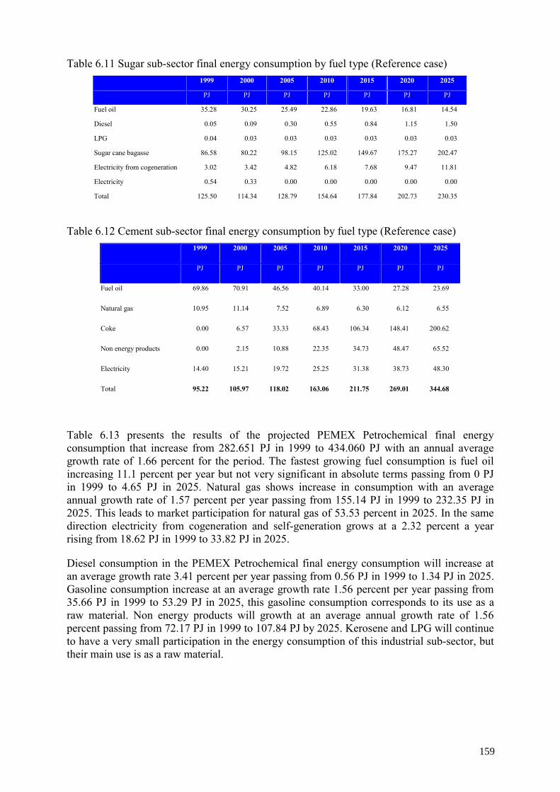
Table 6.11 Sugar sub-sector final energy consumption by fuel type (Reference case) 1999 2000 2005 2010 2015 2020 2025


Fuel oil 35.28 30.25 25.49 22.86 19.63 16.81 14.54

Diesel 0.05 0.09 0.30 0.55 0.84 1.15 1.50

LPG 0.04 0.03 0.03 0.03 0.03 0.03 0.03

Sugar cane bagasse 86.58 80.22 98.15 125.02 149.67 175.27 202.47


Electricity 0.54 0.33 0.00 0.00 0.00 0.00 0.00

Total 125.50 114.34 128.79 154.64 177.84 202.73 230.35

Table 6.12 Cement sub-sector final energy consumption by fuel type (Reference case) 1999 2000 2005 2010 2015 2020 2025


Fuel oil 69.86 70.91 46.56 40.14 33.00 27.28 23.69

Natural gas 10.95 11.14 7.52 6.89 6.30 6.12 6.55

Coke 0.00 6.57 33.33 68.43 106.34 148.41 200.62


Electricity 14.40 15.21 19.72 25.25 31.38 38.73 48.30

Total 95.22 105.97 118.02 163.06 211.75 269.01 344.68

Table 6.13 presents the results of the projected PEMEX Petrochemical final energy consumption that increase from 282.651 PJ in 1999 to 434.060 PJ with an annual average growth rate of 1.66 percent for the period. The fastest growing fuel consumption is fuel oil increasing 11.1 percent per year but not very significant in absolute terms passing from 0 PJ in 1999 to 4.65 PJ in 2025. Natural gas shows increase in consumption with an average annual growth rate of 1.57 percent per year passing from 155.14 PJ in 1999 to 232.35 PJ in 2025. This leads to market participation for natural gas of 53.53 percent in 2025. In the same direction electricity from cogeneration and self-generation grows at a 2.32 percent a year rising from 18.62 PJ in 1999 to 33.82 PJ in 2025.

Diesel consumption in the PEMEX Petrochemical final energy consumption will increase at an average growth rate 3.41 percent per year passing from 0.56 PJ in 1999 to 1.34 PJ in 2025. Gasoline consumption increase at an average growth rate 1.56 percent per year passing from 35.66 PJ in 1999 to 53.29 PJ in 2025, this gasoline consumption corresponds to its use as a raw material. Non energy products will growth at an average annual growth rate of 1.56 percent passing from 72.17 PJ in 1999 to 107.84 PJ by 2025. Kerosene and LPG will continue to have a very small participation in the energy consumption of this industrial sub-sector, but their main use is as a raw material.

159

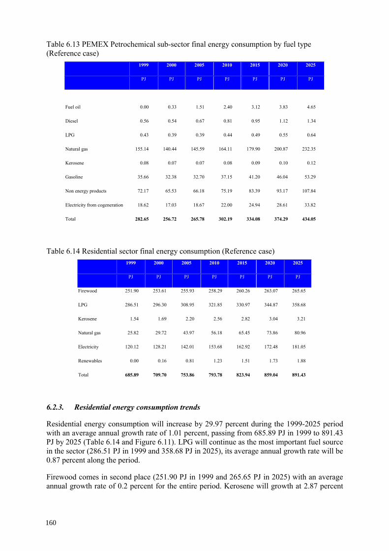
Table 6.13 PEMEX Petrochemical sub-sector final energy consumption by fuel type (Reference case)

1999 2000 2005 2010 2015 2020 2025


Fuel oil 0.00 0.33 1.51 2.40 3.12 3.83 4.65

Diesel 0.56 0.54 0.67 0.81 0.95 1.12 1.34

LPG 0.43 0.39 0.39 0.44 0.49 0.55 0.64

Natural gas 155.14 140.44 145.59 164.11 179.90 200.87 232.35

Kerosene 0.08 0.07 0.07 0.08 0.09 0.10 0.12

Gasoline 35.66 32.38 32.70 37.15 41.20 46.04 53.29



Total 282.65 256.72 265.78 302.19 334.08 374.29 434.05

Table 6.14 Residential sector final energy consumption (Reference case) 1999 2000 2005 2010 2015 2020 2025


Firewood 251.90 253.61 255.93 258.29 260.26 263.07 265.65

LPG 286.51 296.30 308.95 321.85 330.97 344.87 358.68

Kerosene 1.54 1.69 2.20 2.56 2.82 3.04 3.21

Natural gas 25.82 29.72 43.97 56.18 65.45 73.86 80.96

Electricity 120.12 128.21 142.01 153.68 162.92 172.48 181.05

Renewables 0.00 0.16 0.81 1.23 1.51 1.73 1.88

Total 685.89 709.70 753.86 793.78 823.94 859.04 891.43

6.2.3. Residential energy consumption trends

Residential energy consumption will increase by 29.97 percent during the 1999-2025 period with an average annual growth rate of 1.01 percent, passing from 685.89 PJ in 1999 to 891.43 PJ by 2025 (Table 6.14 and Figure 6.11). LPG will continue as the most important fuel source in the sector (286.51 PJ in 1999 and 358.68 PJ in 2025), its average annual growth rate will be 0.87 percent along the period.

Firewood comes in second place (251.90 PJ in 1999 and 265.65 PJ in 2025) with an average annual growth rate of 0.2 percent for the entire period. Kerosene will growth at 2.87 percent

160

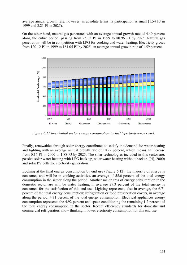
average annual growth rate, however, in absolute terms its participation is small (1.54 PJ in 1999 and 3.21 PJ in 2025).

On the other hand, natural gas penetrates with an average annual growth rate of 4.49 percent along the entire period, passing from 25.82 PJ in 1999 to 80.96 PJ by 2025. Natural gas penetration will be in competition with LPG for cooking and water heating. Electricity grows from 120.12 PJ in 1999 to 181.05 PJ by 2025, an average annual growth rate of 1.59 percent.

0

200

400

600

800

1,000

1,200

1999 2004 2009 2014 2019 2024

Res

iden

tial f

inal

ene

rgy

[PJ]

Wood LPG Kerosene Natural Gas Electricity Renewables

Figure 6.11 Residential sector energy consumption by fuel type (Reference case).

Finally, renewables through solar energy contributes to satisfy the demand for water heating and lighting with an average annual growth rate of 10.22 percent, which means an increase from 0.16 PJ in 2000 to 1.88 PJ by 2025. The solar technologies included in this sector are: passive solar water heating with LPG back-up, solar water heating without backup ([4], 2000) and solar PV cells for electricity generation.

Looking at the final energy consumption by end use (Figure 6.12), the majority of energy is consumed and will be in cooking activities, an average of 55.6 percent of the total energy consumption in the sector along the period. Another major area of energy consumption in the domestic sector are will be water heating, in average 27.3 percent of the total energy is consumed for the satisfaction of this end use. Lighting represents, also in average, the 6.71 percent of the total energy consumption; refrigeration or food preservation covers, in average along the period, 4.31 percent of the total energy consumption. Electrical appliances energy consumption represents the 4.92 percent and space conditioning the remaining 1.2 percent of the total energy consumption in the sector. Recent efficiency standards for domestic and commercial refrigerators allow thinking in lower electricity consumption for this end use.

161

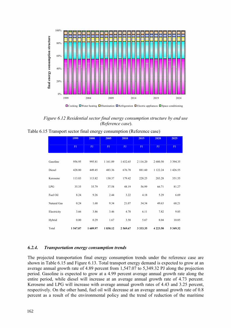
0%

20%

40%

60%

80%

100%

1999 2004 2009 2014 2019 2024

final

ene

rgy

cons

umpt

ion

stru

ctur

e

Cooking Water heating Illumination Refrigeration Electric appliances Space conditioning

Figure 6.12 Residential sector final energy consumption structure by end use (Reference case).

Table 6.15 Transport sector final energy consumption (Reference case) 1999 2000 2005 2010 2015 2020 2025


Gasoline 956.95 995.81 1 161.89 1 632.65 2 116.20 2 680.50 3 394.35

Diesel 428.80 449.45 483.36 676.78 881.60 1 122.24 1 426.55

Kerosene 113.83 113.82 130.37 179.42 228.25 283.28 351.55

LPG 35.35 35.79 37.58 48.19 56.99 66.71 81.27

Fuel Oil 8.24 9.26 2.44 3.22 4.18 5.29 6.69

Natural Gas 0.24 1.68 9.34 21.07 34.34 49.63 68.21

Electricity 3.66 3.86 3.46 4.78 6.11 7.82 9.85

Hybrid 0.00 0.29 1.67 3.58 5.67 8.04 10.85

Total 1 547.07 1 609.97 1 830.12 2 569.67 3 333.35 4 223.50 5 349.32

6.2.4. Transportation energy consumption trends

The projected transportation final energy consumption trends under the reference case are shown in Table 6.15 and Figure 6.13. Total transport energy demand is expected to grow at an average annual growth rate of 4.89 percent from 1,547.07 to 5,349.32 PJ along the projection period. Gasoline is expected to grow at a 4.99 percent average annual growth rate along the entire period, while diesel will increase at an average annual growth rate of 4.73 percent. Kerosene and LPG will increase with average annual growth rates of 4.43 and 3.25 percent, respectively. On the other hand, fuel oil will decrease at an average annual growth rate of 0.8 percent as a result of the environmental policy and the trend of reduction of the maritime

162

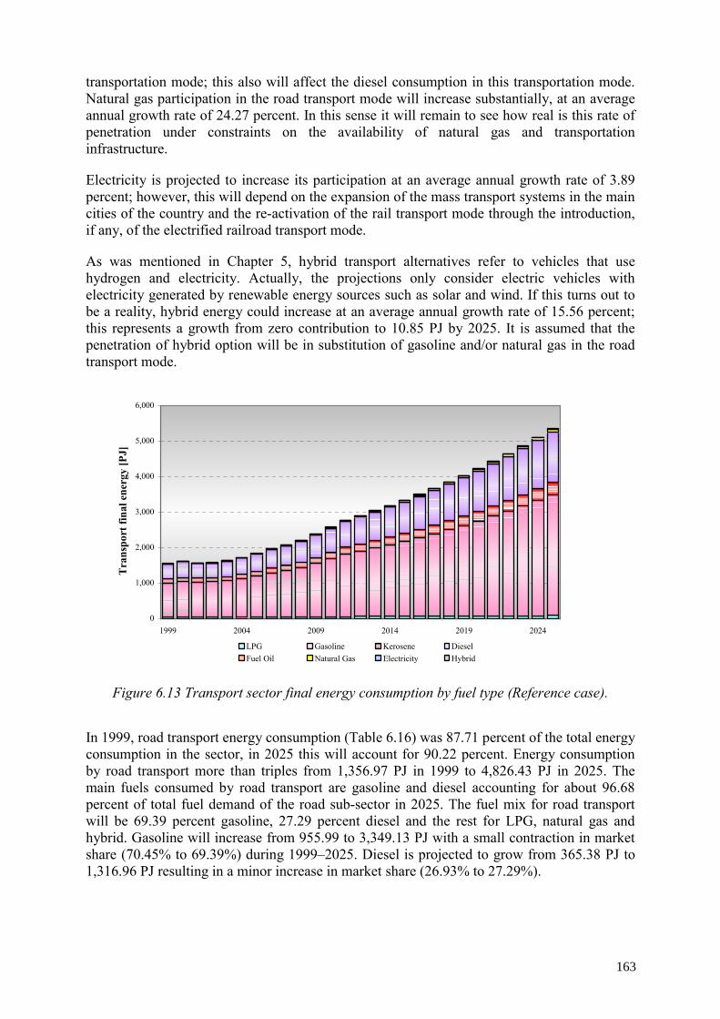
transportation mode; this also will affect the diesel consumption in this transportation mode. Natural gas participation in the road transport mode will increase substantially, at an average annual growth rate of 24.27 percent. In this sense it will remain to see how real is this rate of penetration under constraints on the availability of natural gas and transportation infrastructure.

Electricity is projected to increase its participation at an average annual growth rate of 3.89 percent; however, this will depend on the expansion of the mass transport systems in the main cities of the country and the re-activation of the rail transport mode through the introduction, if any, of the electrified railroad transport mode.

As was mentioned in Chapter 5, hybrid transport alternatives refer to vehicles that use hydrogen and electricity. Actually, the projections only consider electric vehicles with electricity generated by renewable energy sources such as solar and wind. If this turns out to be a reality, hybrid energy could increase at an average annual growth rate of 15.56 percent; this represents a growth from zero contribution to 10.85 PJ by 2025. It is assumed that the penetration of hybrid option will be in substitution of gasoline and/or natural gas in the road transport mode.

0

1,000

2,000

3,000

4,000

5,000

6,000

1999 2004 2009 2014 2019 2024

Tra

nspo

rt fi

nal e

nerg

y [P

J]

LPG Gasoline Kerosene DieselFuel Oil Natural Gas Electricity Hybrid

Figure 6.13 Transport sector final energy consumption by fuel type (Reference case).

In 1999, road transport energy consumption (Table 6.16) was 87.71 percent of the total energy consumption in the sector, in 2025 this will account for 90.22 percent. Energy consumption by road transport more than triples from 1,356.97 PJ in 1999 to 4,826.43 PJ in 2025. The main fuels consumed by road transport are gasoline and diesel accounting for about 96.68 percent of total fuel demand of the road sub-sector in 2025. The fuel mix for road transport will be 69.39 percent gasoline, 27.29 percent diesel and the rest for LPG, natural gas and hybrid. Gasoline will increase from 955.99 to 3,349.13 PJ with a small contraction in market share (70.45% to 69.39%) during 1999–2025. Diesel is projected to grow from 365.38 PJ to 1,316.96 PJ resulting in a minor increase in market share (26.93% to 27.29%).

163

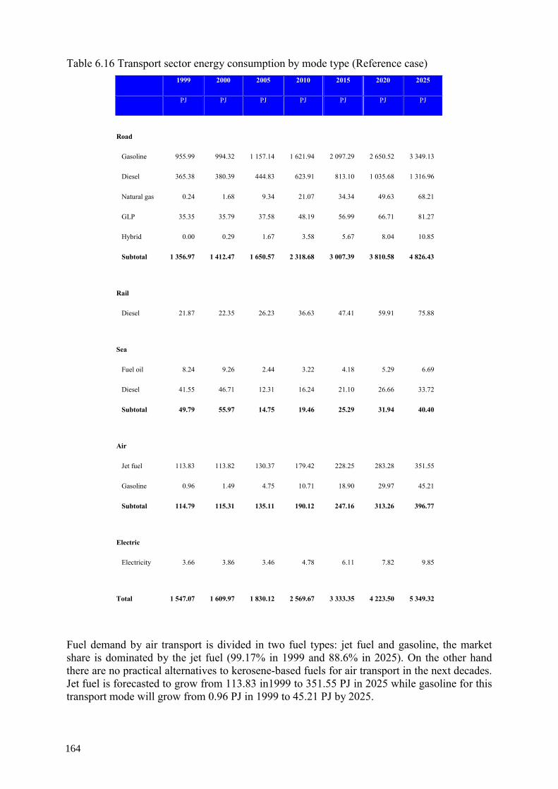
Table 6.16 Transport sector energy consumption by mode type (Reference case) 1999 2000 2005 2010 2015 2020 2025


Road

Gasoline 955.99 994.32 1 157.14 1 621.94 2 097.29 2 650.52 3 349.13

Diesel 365.38 380.39 444.83 623.91 813.10 1 035.68 1 316.96

Natural gas 0.24 1.68 9.34 21.07 34.34 49.63 68.21

GLP 35.35 35.79 37.58 48.19 56.99 66.71 81.27

Hybrid 0.00 0.29 1.67 3.58 5.67 8.04 10.85

Subtotal 1 356.97 1 412.47 1 650.57 2 318.68 3 007.39 3 810.58 4 826.43

Rail

Diesel 21.87 22.35 26.23 36.63 47.41 59.91 75.88

Sea

Fuel oil 8.24 9.26 2.44 3.22 4.18 5.29 6.69

Diesel 41.55 46.71 12.31 16.24 21.10 26.66 33.72

Subtotal 49.79 55.97 14.75 19.46 25.29 31.94 40.40

Air

Jet fuel 113.83 113.82 130.37 179.42 228.25 283.28 351.55

Gasoline 0.96 1.49 4.75 10.71 18.90 29.97 45.21

Subtotal 114.79 115.31 135.11 190.12 247.16 313.26 396.77

Electric

Electricity 3.66 3.86 3.46 4.78 6.11 7.82 9.85

Total 1 547.07 1 609.97 1 830.12 2 569.67 3 333.35 4 223.50 5 349.32

Fuel demand by air transport is divided in two fuel types: jet fuel and gasoline, the market share is dominated by the jet fuel (99.17% in 1999 and 88.6% in 2025). On the other hand there are no practical alternatives to kerosene-based fuels for air transport in the next decades. Jet fuel is forecasted to grow from 113.83 in1999 to 351.55 PJ in 2025 while gasoline for this transport mode will grow from 0.96 PJ in 1999 to 45.21 PJ by 2025.

164

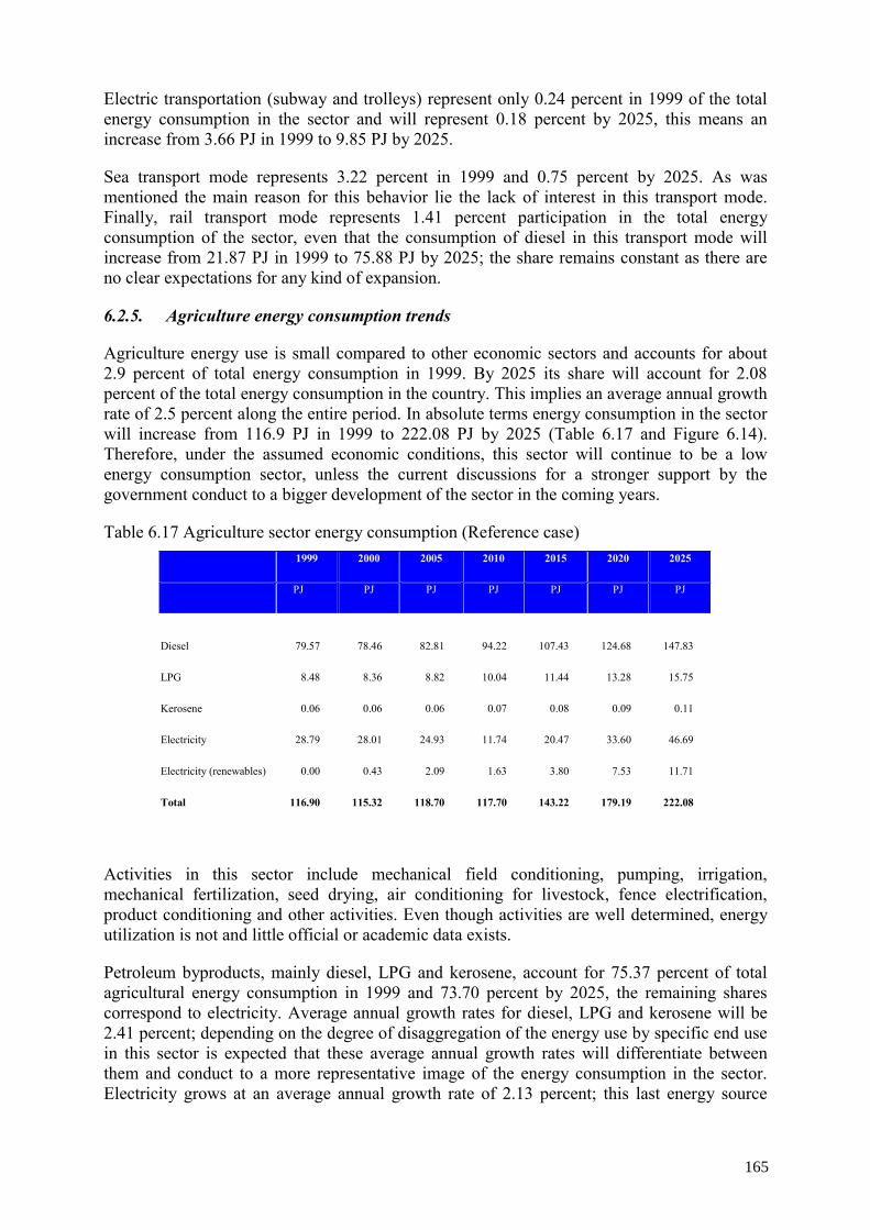
Electric transportation (subway and trolleys) represent only 0.24 percent in 1999 of the total energy consumption in the sector and will represent 0.18 percent by 2025, this means an increase from 3.66 PJ in 1999 to 9.85 PJ by 2025.

Sea transport mode represents 3.22 percent in 1999 and 0.75 percent by 2025. As was mentioned the main reason for this behavior lie the lack of interest in this transport mode. Finally, rail transport mode represents 1.41 percent participation in the total energy consumption of the sector, even that the consumption of diesel in this transport mode will increase from 21.87 PJ in 1999 to 75.88 PJ by 2025; the share remains constant as there are no clear expectations for any kind of expansion.

6.2.5. Agriculture energy consumption trends

Agriculture energy use is small compared to other economic sectors and accounts for about 2.9 percent of total energy consumption in 1999. By 2025 its share will account for 2.08 percent of the total energy consumption in the country. This implies an average annual growth rate of 2.5 percent along the entire period. In absolute terms energy consumption in the sector will increase from 116.9 PJ in 1999 to 222.08 PJ by 2025 (Table 6.17 and Figure 6.14). Therefore, under the assumed economic conditions, this sector will continue to be a low energy consumption sector, unless the current discussions for a stronger support by the government conduct to a bigger development of the sector in the coming years.

Table 6.17 Agriculture sector energy consumption (Reference case) 1999 2000 2005 2010 2015 2020 2025


Diesel 79.57 78.46 82.81 94.22 107.43 124.68 147.83

LPG 8.48 8.36 8.82 10.04 11.44 13.28 15.75

Kerosene 0.06 0.06 0.06 0.07 0.08 0.09 0.11

Electricity 28.79 28.01 24.93 11.74 20.47 33.60 46.69

Electricity (renewables) 0.00 0.43 2.09 1.63 3.80 7.53 11.71

Total 116.90 115.32 118.70 117.70 143.22 179.19 222.08

Activities in this sector include mechanical field conditioning, pumping, irrigation, mechanical fertilization, seed drying, air conditioning for livestock, fence electrification, product conditioning and other activities. Even though activities are well determined, energy utilization is not and little official or academic data exists.

Petroleum byproducts, mainly diesel, LPG and kerosene, account for 75.37 percent of total agricultural energy consumption in 1999 and 73.70 percent by 2025, the remaining shares correspond to electricity. Average annual growth rates for diesel, LPG and kerosene will be 2.41 percent; depending on the degree of disaggregation of the energy use by specific end use in this sector is expected that these average annual growth rates will differentiate between them and conduct to a more representative image of the energy consumption in the sector. Electricity grows at an average annual growth rate of 2.13 percent; this last energy source

165

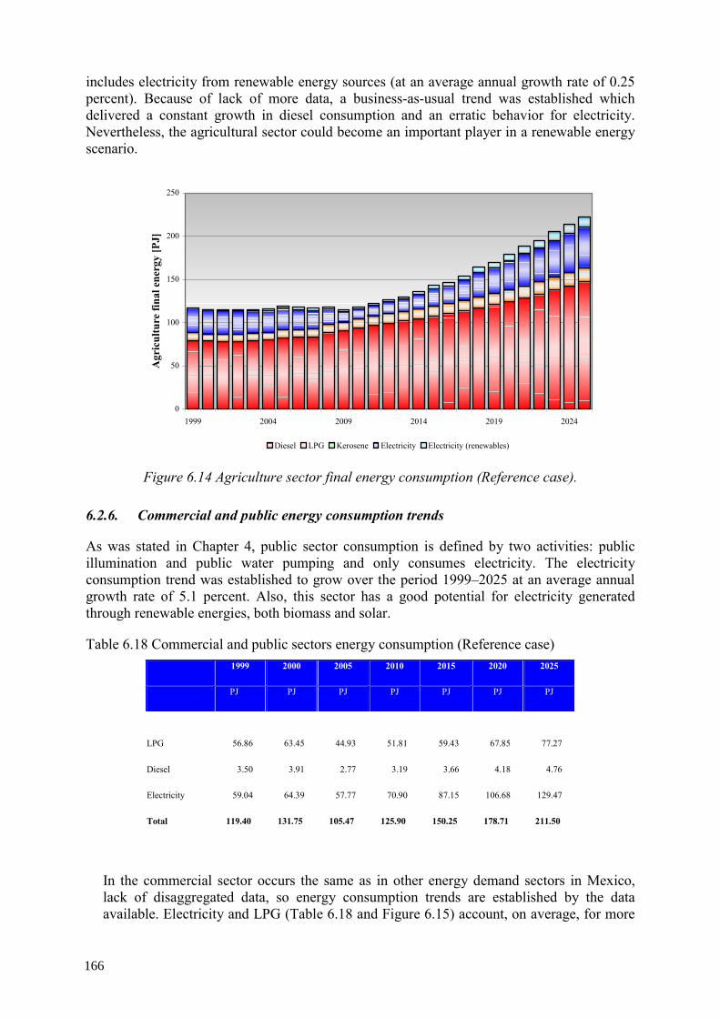
includes electricity from renewable energy sources (at an average annual growth rate of 0.25 percent). Because of lack of more data, a business-as-usual trend was established which delivered a constant growth in diesel consumption and an erratic behavior for electricity. Nevertheless, the agricultural sector could become an important player in a renewable energy scenario.

0

50

100

150

200

250

1999 2004 2009 2014 2019 2024

Agr

icul

ture

fina

l ene

rgy

[PJ]

Diesel LPG Kerosene Electricity Electricity (renewables)

Figure 6.14 Agriculture sector final energy consumption (Reference case).

6.2.6. Commercial and public energy consumption trends

As was stated in Chapter 4, public sector consumption is defined by two activities: public illumination and public water pumping and only consumes electricity. The electricity consumption trend was established to grow over the period 1999–2025 at an average annual growth rate of 5.1 percent. Also, this sector has a good potential for electricity generated through renewable energies, both biomass and solar.

Table 6.18 Commercial and public sectors energy consumption (Reference case) 1999 2000 2005 2010 2015 2020 2025


LPG 56.86 63.45 44.93 51.81 59.43 67.85 77.27

Diesel 3.50 3.91 2.77 3.19 3.66 4.18 4.76

Electricity 59.04 64.39 57.77 70.90 87.15 106.68 129.47

Total 119.40 131.75 105.47 125.90 150.25 178.71 211.50

In the commercial sector occurs the same as in other energy demand sectors in Mexico, lack of disaggregated data, so energy consumption trends are established by the data available. Electricity and LPG (Table 6.18 and Figure 6.15) account, on average, for more

166

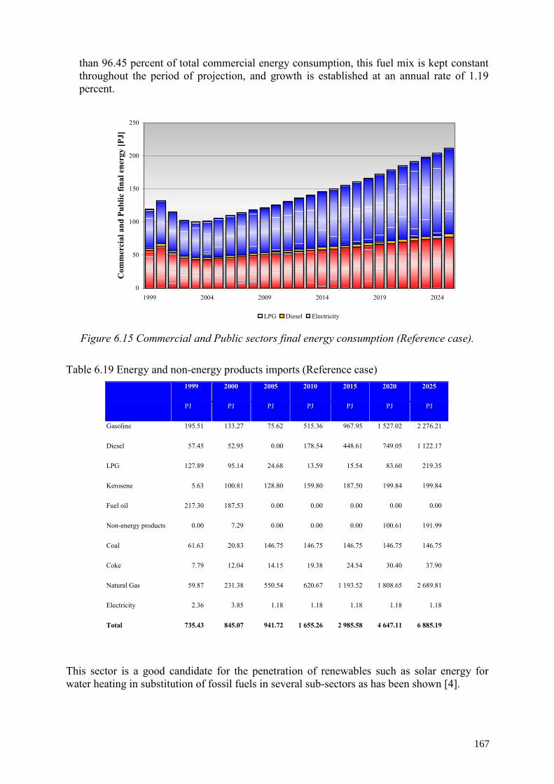
than 96.45 percent of total commercial energy consumption, this fuel mix is kept constant throughout the period of projection, and growth is established at an annual rate of 1.19 percent.

0

50

100

150

200

250

1999 2004 2009 2014 2019 2024

Com

mer

cial

and

Pub

lic fi

nal e

nerg

y [P

J]

LPG Diesel Electricity

Figure 6.15 Commercial and Public sectors final energy consumption (Reference case).

Table 6.19 Energy and non-energy products imports (Reference case) 1999 2000 2005 2010 2015 2020 2025


Gasoline 195.51 133.27 75.62 515.36 967.95 1 527.02 2 276.21

Diesel 57.45 52.95 0.00 178.54 448.61 749.05 1 122.17

LPG 127.89 95.14 24.68 13.59 15.54 83.60 219.35

Kerosene 5.63 100.81 128.80 159.80 187.50 199.84 199.84

Fuel oil 217.30 187.53 0.00 0.00 0.00 0.00 0.00


Coal 61.63 20.83 146.75 146.75 146.75 146.75 146.75

Coke 7.79 12.04 14.15 19.38 24.54 30.40 37.90

Natural Gas 59.87 231.38 550.54 620.67 1 193.52 1 808.65 2 689.81

Electricity 2.36 3.85 1.18 1.18 1.18 1.18 1.18

Total 735.43 845.07 941.72 1 655.26 2 985.58 4 647.11 6 885.19

This sector is a good candidate for the penetration of renewables such as solar energy for water heating in substitution of fossil fuels in several sub-sectors as has been shown [4].

167

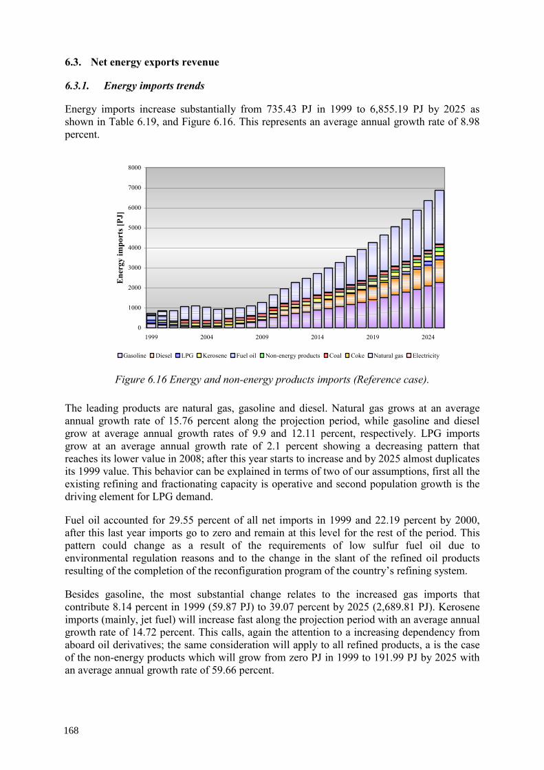
6.3. Net energy exports revenue

6.3.1. Energy imports trends

Energy imports increase substantially from 735.43 PJ in 1999 to 6,855.19 PJ by 2025 as shown in Table 6.19, and Figure 6.16. This represents an average annual growth rate of 8.98 percent.

0

1000

2000

3000

4000

5000

6000

7000

8000

1999 2004 2009 2014 2019 2024

Ene

rgy

impo

rts [

PJ]

Gasoline Diesel LPG Kerosene Fuel oil Non-energy products Coal Coke Natural gas Electricity

Figure 6.16 Energy and non-energy products imports (Reference case).

The leading products are natural gas, gasoline and diesel. Natural gas grows at an average annual growth rate of 15.76 percent along the projection period, while gasoline and diesel grow at average annual growth rates of 9.9 and 12.11 percent, respectively. LPG imports grow at an average annual growth rate of 2.1 percent showing a decreasing pattern that reaches its lower value in 2008; after this year starts to increase and by 2025 almost duplicates its 1999 value. This behavior can be explained in terms of two of our assumptions, first all the existing refining and fractionating capacity is operative and second population growth is the driving element for LPG demand.

Fuel oil accounted for 29.55 percent of all net imports in 1999 and 22.19 percent by 2000, after this last year imports go to zero and remain at this level for the rest of the period. This pattern could change as a result of the requirements of low sulfur fuel oil due to environmental regulation reasons and to the change in the slant of the refined oil products resulting of the completion of the reconfiguration program of the country’s refining system.

Besides gasoline, the most substantial change relates to the increased gas imports that contribute 8.14 percent in 1999 (59.87 PJ) to 39.07 percent by 2025 (2,689.81 PJ). Kerosene imports (mainly, jet fuel) will increase fast along the projection period with an average annual growth rate of 14.72 percent. This calls, again the attention to a increasing dependency from aboard oil derivatives; the same consideration will apply to all refined products, a is the case of the non-energy products which will grow from zero PJ in 1999 to 191.99 PJ by 2025 with an average annual growth rate of 59.66 percent.

168

Coal, thermal and metallurgical will increase also due to requirements of the iron and steel industry as well as those associated with the shifting from fuel oil to imported coal in the dual power plants. The expected average annual growth rate for coal is 3.39 percent along the entire period. Coal imports will increase from 61.63 PJ in 1999 to 146.75 percent in 2025.

Coke imports will grow, at an average annual growth rate of 6.27 percent, from 7.79 PJ in 1999 to 37.90 PJ by 2025. Finally, electricity imports will remain small and, as matter of fact, they will decrease, at an average annual growth rate of 2.64 percent, from 2.18 PJ in 1999 to 1.18 PJ by 2025.

6.3.2. Energy imports trends

Total energy exports projections pass from 3,730.68 PJ in 1999 to 4,806.6 PJ by 2025 (Table 6.20 and Figure 6.17) with an average annual growth rate of 0.98 percent. Crude oil exports will continue to be the most important energy export (on the average a 94.48 percent of the total energy exports), in 1999 crude oil exports account for 3,396.07 PJ and is projected, by 2025, to arose to 4,519.78 PJ in the reference case; which means an average annual growth rate of 1.11 percent. Natural gas losses market share in the exports (from 1.32 percent in 1999 to 0.12 percent in 2025) at an average annual growth rate of 7.96 percent. However, the natural gas entire picture, imports and exports, will change if the investments in natural gas extraction, processing and fractionating capacities commented in section 5.1.2 become real.

Table 6.20 Energy and non-energy products exports (Reference case) 1999 2000 2005 2010 2015 2020 2025


Crude oil 3 396.07 3 631.76 3 897.48 4 083.73 4 246.34 4 390.52 4 519.78

Natural gas 49.41 8.65 8.10 7.40 6.80 6.24 5.73

Gasoline 134.08 118.12 139.65 159.95 174.68 186.24 213.26

Diesel 18.86 9.34 20.79 21.83 22.74 23.55 24.28

LPG 5.91 7.35 4.33 4.55 4.74 4.91 5.07

Kerosene 4.80 7.50 5.35 5.63 5.88 6.11 6.31

Coke 0.02 0.05 0.03 0.03 0.03 0.03 0.04

Electricity 0.47 0.70 1.02 1.07 1.12 1.16 1.20


Total 3 617.10 3 796.71 4 086.66 4 294.59 4 473.16 4 629.98 4 787.24

Gasoline exports grow at an average annual growth rate of 1.18 percent implying an increase from 134.08 PJ in 1999 to 213.26 PJ by 2025. Diesel exports also increase, but an average annual growth rate of 0.98 percent passing from 18.86 PJ in 1999 to 24.28 PJ by 2025.

169

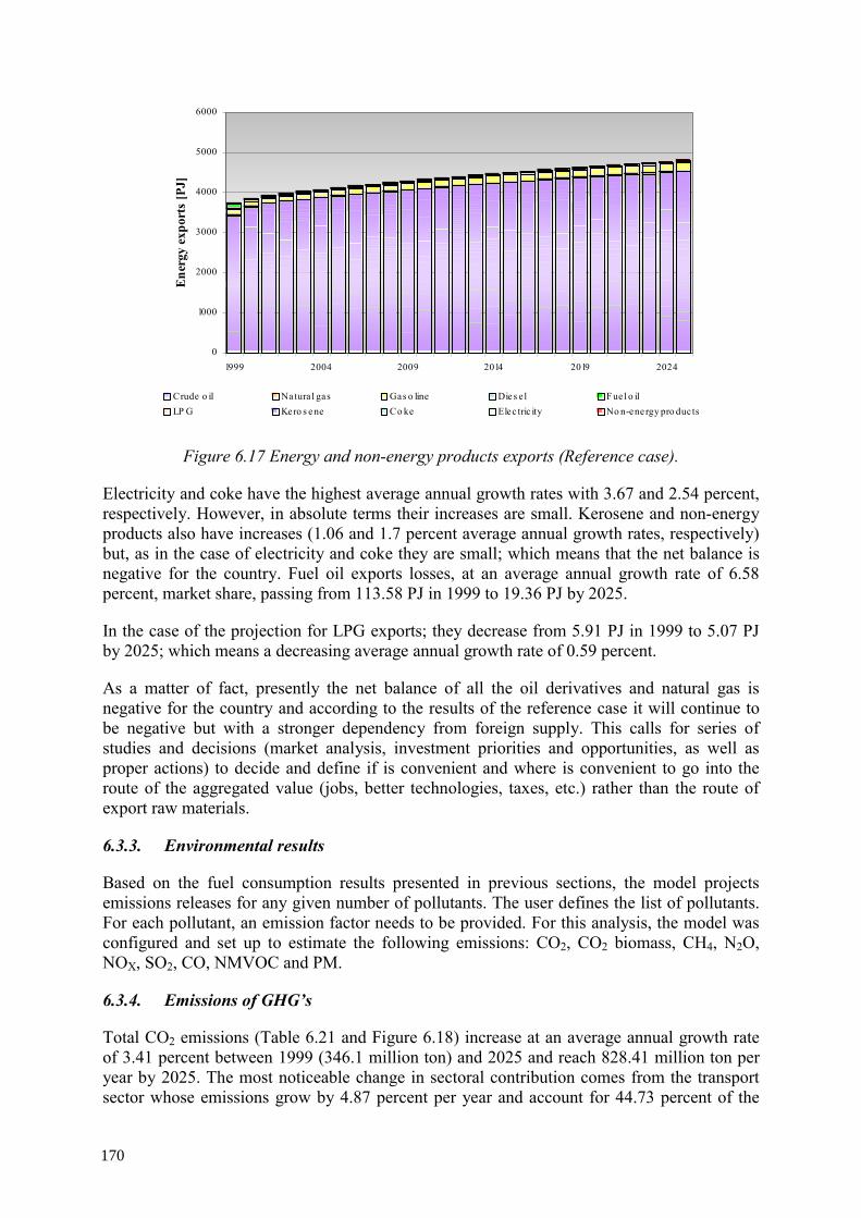
0

1000

2000

3000

4000

5000

6000

1999 2004 2009 2014 2019 2024

Ene

rgy

expo

rts

[PJ]

Crude o il Natura l gas Gas o line Die s e l Fuel o ilLP G Kero s e ne Co ke Elec tric ity No n-ene rgy pro ducts

Figure 6.17 Energy and non-energy products exports (Reference case).

Electricity and coke have the highest average annual growth rates with 3.67 and 2.54 percent, respectively. However, in absolute terms their increases are small. Kerosene and non-energy products also have increases (1.06 and 1.7 percent average annual growth rates, respectively) but, as in the case of electricity and coke they are small; which means that the net balance is negative for the country. Fuel oil exports losses, at an average annual growth rate of 6.58 percent, market share, passing from 113.58 PJ in 1999 to 19.36 PJ by 2025.

In the case of the projection for LPG exports; they decrease from 5.91 PJ in 1999 to 5.07 PJ by 2025; which means a decreasing average annual growth rate of 0.59 percent.

As a matter of fact, presently the net balance of all the oil derivatives and natural gas is negative for the country and according to the results of the reference case it will continue to be negative but with a stronger dependency from foreign supply. This calls for series of studies and decisions (market analysis, investment priorities and opportunities, as well as proper actions) to decide and define if is convenient and where is convenient to go into the route of the aggregated value (jobs, better technologies, taxes, etc.) rather than the route of export raw materials.

6.3.3. Environmental results

Based on the fuel consumption results presented in previous sections, the model projects emissions releases for any given number of pollutants. The user defines the list of pollutants. For each pollutant, an emission factor needs to be provided. For this analysis, the model was configured and set up to estimate the following emissions: CO2, CO2 biomass, CH4, N2O, NOX, SO2, CO, NMVOC and PM.

6.3.4. Emissions of GHG’s

Total CO2 emissions (Table 6.21 and Figure 6.18) increase at an average annual growth rate of 3.41 percent between 1999 (346.1 million ton) and 2025 and reach 828.41 million ton per year by 2025. The most noticeable change in sectoral contribution comes from the transport sector whose emissions grow by 4.87 percent per year and account for 44.73 percent of the

170

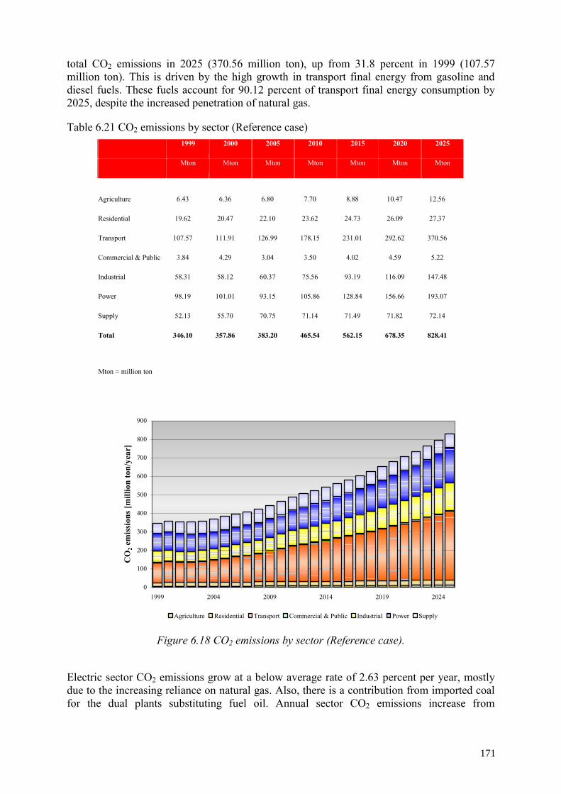
total CO2 emissions in 2025 (370.56 million ton), up from 31.8 percent in 1999 (107.57 million ton). This is driven by the high growth in transport final energy from gasoline and diesel fuels. These fuels account for 90.12 percent of transport final energy consumption by 2025, despite the increased penetration of natural gas.

Table 6.21 CO2 emissions by sector (Reference case) 1999 2000 2005 2010 2015 2020 2025

Mton Mton Mton Mton Mton Mton Mton

Agriculture 6.43 6.36 6.80 7.70 8.88 10.47 12.56

Residential 19.62 20.47 22.10 23.62 24.73 26.09 27.37

Transport 107.57 111.91 126.99 178.15 231.01 292.62 370.56

Commercial & Public 3.84 4.29 3.04 3.50 4.02 4.59 5.22

Industrial 58.31 58.12 60.37 75.56 93.19 116.09 147.48

Power 98.19 101.01 93.15 105.86 128.84 156.66 193.07

Supply 52.13 55.70 70.75 71.14 71.49 71.82 72.14

Total 346.10 357.86 383.20 465.54 562.15 678.35 828.41

Mton = million ton

0

100

200

300

400

500

600

700

800

900

1999 2004 2009 2014 2019 2024

CO

2 em

issi

ons [

mill

ion

ton/

year

]

Agriculture Residential Transport Commercial & Public Industrial Power Supply

Figure 6.18 CO2 emissions by sector (Reference case).

Electric sector CO2 emissions grow at a below average rate of 2.63 percent per year, mostly due to the increasing reliance on natural gas. Also, there is a contribution from imported coal for the dual plants substituting fuel oil. Annual sector CO2 emissions increase from

171

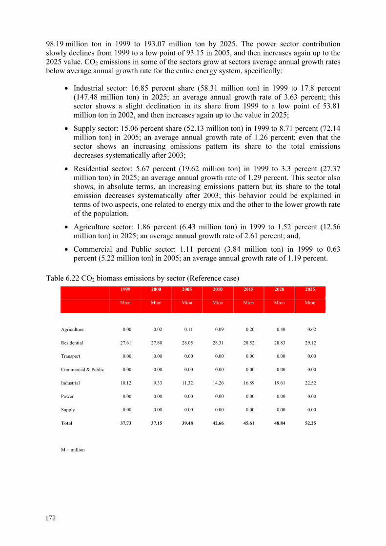
98.19 million ton in 1999 to 193.07 million ton by 2025. The power sector contribution slowly declines from 1999 to a low point of 93.15 in 2005, and then increases again up to the 2025 value. CO2 emissions in some of the sectors grow at sectors average annual growth rates below average annual growth rate for the entire energy system, specifically:

• Industrial sector: 16.85 percent share (58.31 million ton) in 1999 to 17.8 percent (147.48 million ton) in 2025; an average annual growth rate of 3.63 percent; this sector shows a slight declination in its share from 1999 to a low point of 53.81 million ton in 2002, and then increases again up to the value in 2025;

• Supply sector: 15.06 percent share (52.13 million ton) in 1999 to 8.71 percent (72.14 million ton) in 2005; an average annual growth rate of 1.26 percent; even that the sector shows an increasing emissions pattern its share to the total emissions decreases systematically after 2003;

• Residential sector: 5.67 percent (19.62 million ton) in 1999 to 3.3 percent (27.37 million ton) in 2025; an average annual growth rate of 1.29 percent. This sector also shows, in absolute terms, an increasing emissions pattern but its share to the total emission decreases systematically after 2003; this behavior could be explained in terms of two aspects, one related to energy mix and the other to the lower growth rate of the population.

• Agriculture sector: 1.86 percent (6.43 million ton) in 1999 to 1.52 percent (12.56 million ton) in 2025; an average annual growth rate of 2.61 percent; and,

• Commercial and Public sector: 1.11 percent (3.84 million ton) in 1999 to 0.63 percent (5.22 million ton) in 2005; an average annual growth rate of 1.19 percent.

Table 6.22 CO2 biomass emissions by sector (Reference case) 1999 2000 2005 2010 2015 2020 2025

Mton Mton Mton Mton Mton Mton Mton

Agriculture 0.00 0.02 0.11 0.09 0.20 0.40 0.62

Residential 27.61 27.80 28.05 28.31 28.52 28.83 29.12

Transport 0.00 0.00 0.00 0.00 0.00 0.00 0.00


Industrial 10.12 9.33 11.32 14.26 16.89 19.61 22.52

Power 0.00 0.00 0.00 0.00 0.00 0.00 0.00

Supply 0.00 0.00 0.00 0.00 0.00 0.00 0.00

Total 37.73 37.15 39.48 42.66 45.61 48.84 52.25

M = million

172

As a general result for all the sectors, the decreasing pattern of energy consumption and associated emissions in the years 1999-2003 is a result of the low economic growth of the whole economy.

Following the IPCC methodology, CO2 emissions from the biomass consumption (firewood and sugar cane bagasse in the case of Mexico) are not added to total emission shown in Table 6.21 and Figure 6.18. However, the model allows calculating the CO2 emission originated from the biomass consumption. Table 6.22 and Figure 6.19 show the total amount and the sectoral distribution of the CO2 emissions originated from the use of the firewood in the residential sector for coking and water heating activities and the use of sugar cane bagasse in the sugar industry for the generation of heat process and other uses.

Total CH4 emissions increase by 93.16 percent from 179.39 to 346.5 thousand ton over the period 1999–2025 (Table 6.23, and Figure 6.20), an average annual growth rate of 2.56 percent along the entire period. The main contribution comes from the supply sector with an increase of 2.77 percent per year (103.33 percent total growth) driven by the growth in the coal use. By 2025, the supply sector accounts for 59.76 percent of total CH4 emissions, up from 56.77 percent in 1999. This is followed by the transport sector with a 4.92 percent per year increase, from 21.53 to 75.07 thousand ton, equivalent to a 248.62 percent total increase by the consumption of gasoline and diesel; residential sector emissions growth from 53.23 thousand ton in 1999 to 56.26 thousand ton by 2025 with an average annual growth rate of 0.21 percent. Even that the power sector is projected to have an important increase in the use of natural gas its CH4 emissions do not grow as fast as in other sectors, power sector CH4 emissions grow at an average annual growth rate of 3.8 percent passing from 1.26 thousand ton in 1999 to 3.3 thousand ton in 2025, however in all cases has to be take into account the Direct Global Warming Potential factor for methane and NOX.

0

10

20

30

40

50

60

1999 2004 2009 2014 2019 2024

CO

2 bio

mas

s em

issi

ons [

mill

ion

ton/

year

]


Figure 6.19 CO2 biomass emissions by sector (Reference case).

The industrial and the Commercial and Public sectors show a similar pattern as the power sector, that is, an average annual growth rate of 2.8 and 1.19 percent, respectively, however in

173

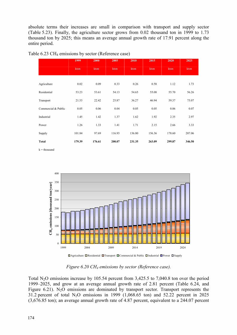
absolute terms their increases are small in comparison with transport and supply sector (Table 5.23). Finally, the agriculture sector grows from 0.02 thousand ton in 1999 to 1.73 thousand ton by 2025; this means an average annual growth rate of 17.91 percent along the entire period.

Table 6.23 CH4 emissions by sector (Reference case) 1999 2000 2005 2010 2015 2020 2025

kton kton kton kton kton kton kton

Agriculture 0.02 0.09 0.33 0.26 0.58 1.12 1.73

Residential 53.23 53.61 54.13 54.65 55.08 55.70 56.26

Transport 21.53 22.42 25.87 36.27 46.94 59.37 75.07


Industrial 1.45 1.42 1.37 1.62 1.92 2.35 2.97

Power 1.26 1.33 1.41 1.71 2.15 2.66 3.33

Supply 101.84 97.69 116.93 136.80 156.36 178.60 207.06

Total 179.39 176.61 200.07 231.35 263.09 299.87 346.50

k = thousand

0

50

100

150

200

250

300

350

400

1999 2004 2009 2014 2019 2024

CH

4 em

issi

ons [

thou

sand

ton/

year

]


Figure 6.20 CH4 emissions by sector (Reference case).

Total N2O emissions increase by 105.54 percent from 3,425.5 to 7,040.8 ton over the period 1999–2025, and grow at an average annual growth rate of 2.81 percent (Table 6.24, and Figure 6.21). N2O emissions are dominated by transport sector. Transport represents the 31.2 percent of total N2O emissions in 1999 (1,068.65 ton) and 52.22 percent in 2025 (3,676.85 ton); an average annual growth rate of 4.87 percent, equivalent to a 244.07 percent

174

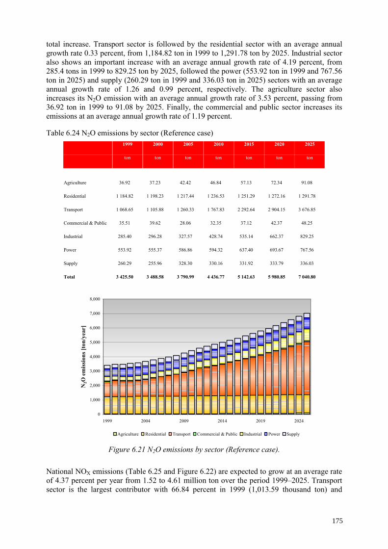
total increase. Transport sector is followed by the residential sector with an average annual growth rate 0.33 percent, from 1,184.82 ton in 1999 to 1,291.78 ton by 2025. Industrial sector also shows an important increase with an average annual growth rate of 4.19 percent, from 285.4 tons in 1999 to 829.25 ton by 2025, followed the power (553.92 ton in 1999 and 767.56 ton in 2025) and supply (260.29 ton in 1999 and 336.03 ton in 2025) sectors with an average annual growth rate of 1.26 and 0.99 percent, respectively. The agriculture sector also increases its N2O emission with an average annual growth rate of 3.53 percent, passing from 36.92 ton in 1999 to 91.08 by 2025. Finally, the commercial and public sector increases its emissions at an average annual growth rate of 1.19 percent.

Table 6.24 N2O emissions by sector (Reference case) 1999 2000 2005 2010 2015 2020 2025

ton ton ton ton ton ton ton

Agriculture 36.92 37.23 42.42 46.84 57.13 72.34 91.08

Residential 1 184.82 1 198.23 1 217.44 1 236.53 1 251.29 1 272.16 1 291.78

Transport 1 068.65 1 105.88 1 260.33 1 767.83 2 292.64 2 904.15 3 676.85


Industrial 285.40 296.28 327.57 428.74 535.14 662.37 829.25

Power 553.92 555.37 586.86 594.32 637.40 693.67 767.56

Supply 260.29 255.96 328.30 330.16 331.92 333.79 336.03

Total 3 425.50 3 488.58 3 790.99 4 436.77 5 142.63 5 980.85 7 040.80

0

1,000

2,000

3,000

4,000

5,000

6,000

7,000

8,000

1999 2004 2009 2014 2019 2024

N2O

em

issi

ons [

ton/

year

]


Figure 6.21 N2O emissions by sector (Reference case).

National NOX emissions (Table 6.25 and Figure 6.22) are expected to grow at an average rate of 4.37 percent per year from 1.52 to 4.61 million ton over the period 1999–2025. Transport sector is the largest contributor with 66.84 percent in 1999 (1,013.59 thousand ton) and

175

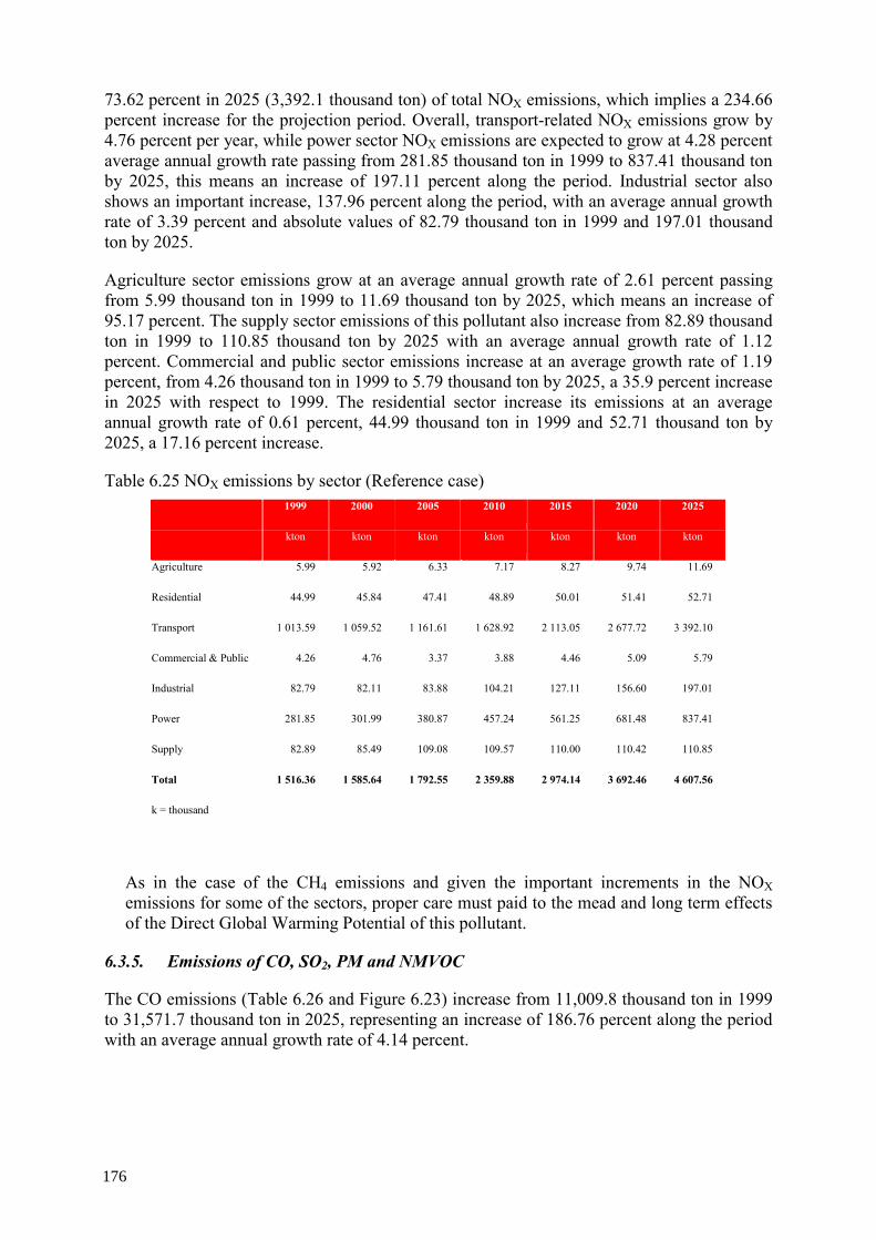
73.62 percent in 2025 (3,392.1 thousand ton) of total NOX emissions, which implies a 234.66 percent increase for the projection period. Overall, transport-related NOX emissions grow by 4.76 percent per year, while power sector NOX emissions are expected to grow at 4.28 percent average annual growth rate passing from 281.85 thousand ton in 1999 to 837.41 thousand ton by 2025, this means an increase of 197.11 percent along the period. Industrial sector also shows an important increase, 137.96 percent along the period, with an average annual growth rate of 3.39 percent and absolute values of 82.79 thousand ton in 1999 and 197.01 thousand ton by 2025.

Agriculture sector emissions grow at an average annual growth rate of 2.61 percent passing from 5.99 thousand ton in 1999 to 11.69 thousand ton by 2025, which means an increase of 95.17 percent. The supply sector emissions of this pollutant also increase from 82.89 thousand ton in 1999 to 110.85 thousand ton by 2025 with an average annual growth rate of 1.12 percent. Commercial and public sector emissions increase at an average growth rate of 1.19 percent, from 4.26 thousand ton in 1999 to 5.79 thousand ton by 2025, a 35.9 percent increase in 2025 with respect to 1999. The residential sector increase its emissions at an average annual growth rate of 0.61 percent, 44.99 thousand ton in 1999 and 52.71 thousand ton by 2025, a 17.16 percent increase.

Table 6.25 NOX emissions by sector (Reference case) 1999 2000 2005 2010 2015 2020 2025


Agriculture 5.99 5.92 6.33 7.17 8.27 9.74 11.69

Residential 44.99 45.84 47.41 48.89 50.01 51.41 52.71

Transport 1 013.59 1 059.52 1 161.61 1 628.92 2 113.05 2 677.72 3 392.10


Industrial 82.79 82.11 83.88 104.21 127.11 156.60 197.01

Power 281.85 301.99 380.87 457.24 561.25 681.48 837.41

Supply 82.89 85.49 109.08 109.57 110.00 110.42 110.85

Total 1 516.36 1 585.64 1 792.55 2 359.88 2 974.14 3 692.46 4 607.56

k = thousand

As in the case of the CH4 emissions and given the important increments in the NOX emissions for some of the sectors, proper care must paid to the mead and long term effects of the Direct Global Warming Potential of this pollutant.

6.3.5. Emissions of CO, SO2, PM and NMVOC

The CO emissions (Table 6.26 and Figure 6.23) increase from 11,009.8 thousand ton in 1999 to 31,571.7 thousand ton in 2025, representing an increase of 186.76 percent along the period with an average annual growth rate of 4.14 percent.

176

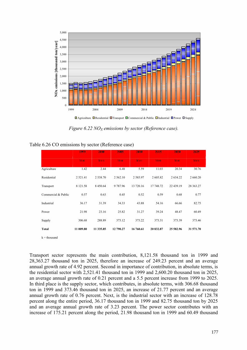
0

500

1,000

1,500

2,000

2,500

3,000

3,500

4,000

4,500

5,000

1999 2004 2009 2014 2019 2024

NO

x em

issi

ons [

thou

sand

ton/

year

]


Figure 6.22 NOX emissions by sector (Reference case).

Table 6.26 CO emissions by sector (Reference case) 1999 2000 2005 2010 2015 2020 2025


Agriculture 1.42 2.44 6.48 5.59 11.03 20.34 30.76

Residential 2 521.41 2 538.70 2 562.10 2 585.97 2 605.82 2 634.22 2 660.20

Transport 8 121.58 8 450.64 9 787.96 13 720.16 17 748.72 22 439.19 28 363.27


Industrial 36.17 31.39 34.33 43.88 54.16 66.66 82.75

Power 21.98 23.16 25.82 31.27 39.24 48.47 60.49

Supply 306.68 288.89 373.12 373.22 373.31 373.39 373.46

Total 11 009.80 11 335.85 12 790.27 16 760.61 20 832.87 25 582.96 31 571.70

k = thousand

Transport sector represents the main contribution, 8,121.58 thousand ton in 1999 and 28,363.27 thousand ton in 2025, therefore an increase of 249.23 percent and an average annual growth rate of 4.92 percent. Second in importance of contribution, in absolute terms, is the residential sector with 2,521.41 thousand ton in 1999 and 2,600.20 thousand ton in 2025, an average annual growth rate of 0.21 percent and a 5.5 percent increase from 1999 to 2025. In third place is the supply sector, which contributes, in absolute terms, with 306.68 thousand ton in 1999 and 373.46 thousand ton in 2025, an increase of 21.77 percent and an average annual growth rate of 0.76 percent. Next, is the industrial sector with an increase of 128.78 percent along the entire period, 36.17 thousand ton in 1999 and 82.75 thousand ton by 2025 and an average annual growth rate of 3.23 percent. The power sector contributes with an increase of 175.21 percent along the period, 21.98 thousand ton in 1999 and 60.49 thousand

177

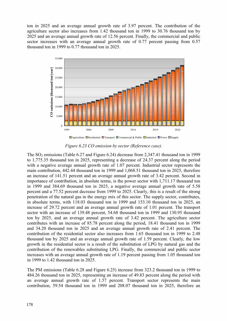
ton in 2025 and an average annual growth rate of 3.97 percent. The contribution of the agriculture sector also increases from 1.42 thousand ton in 1999 to 30.76 thousand ton by 2025 and an average annual growth rate of 12.56 percent. Finally, the commercial and public sector increases with an average annual growth rate of 0.77 percent passing from 0.57 thousand ton in 1999 to 0.77 thousand ton in 2025.

0

5,000

10,000

15,000

20,000

25,000

30,000

35,000

1999 2004 2009 2014 2019 2024

CO

em

issi

ons [

thou

sand

ton/

year

]


Figure 6.23 CO emission by sector (Reference case).

The SO2 emissions (Table 6.27 and Figure 6.24) decrease from 2,347.41 thousand ton in 1999 to 1,775.35 thousand ton in 2025, representing a decrease of 24.37 percent along the period with a negative average annual growth rate of 1.07 percent. Industrial sector represents the main contribution, 442.44 thousand ton in 1999 and 1,068.51 thousand ton in 2025, therefore an increase of 141.51 percent and an average annual growth rate of 3.42 percent. Second in importance of contribution, in absolute terms, is the power sector with 1,711.17 thousand ton in 1999 and 384.69 thousand ton in 2025, a negative average annual growth rate of 5.58 percent and a 77.52 percent decrease from 1999 to 2025. Clearly, this is a result of the strong penetration of the natural gas in the energy mix of this sector. The supply sector, contributes, in absolute terms, with 118.03 thousand ton in 1999 and 153.10 thousand ton in 2025, an increase of 29.72 percent and an average annual growth rate of 1.01 percent. The transport sector with an increase of 139.48 percent, 54.68 thousand ton in 1999 and 130.95 thousand ton by 2025, and an average annual growth rate of 3.42 percent. The agriculture sector contributes with an increase of 85.78 percent along the period, 18.41 thousand ton in 1999 and 34.20 thousand ton in 2025 and an average annual growth rate of 2.41 percent. The contribution of the residential sector also increases from 1.65 thousand ton in 1999 to 2.48 thousand ton by 2025 and an average annual growth rate of 1.59 percent. Clearly, the low growth in the residential sector is a result of the substitution of LPG by natural gas and the contribution of the renewables substituting LPG. Finally, the commercial and public sector increases with an average annual growth rate of 1.19 percent passing from 1.05 thousand ton in 1999 to 1.42 thousand ton in 2025.

The PM emissions (Table 6.28 and Figure 6.25) increase from 323.2 thousand ton in 1999 to 484.26 thousand ton in 2025, representing an increase of 49.83 percent along the period with an average annual growth rate of 1.57 percent. Transport sector represents the main contribution, 59.54 thousand ton in 1999 and 208.07 thousand ton in 2025, therefore an

178

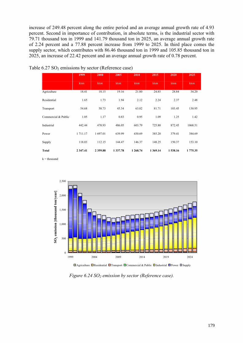
increase of 249.48 percent along the entire period and an average annual growth rate of 4.93 percent. Second in importance of contribution, in absolute terms, is the industrial sector with 79.71 thousand ton in 1999 and 141.79 thousand ton in 2025, an average annual growth rate of 2.24 percent and a 77.88 percent increase from 1999 to 2025. In third place comes the supply sector, which contributes with 86.46 thousand ton in 1999 and 105.85 thousand ton in 2025, an increase of 22.42 percent and an average annual growth rate of 0.78 percent.

Table 6.27 SO2 emissions by sector (Reference case) 1999 2000 2005 2010 2015 2020 2025


Agriculture 18.41 18.15 19.16 21.80 24.85 28.84 34.20

Residential 1.65 1.73 1.94 2.12 2.24 2.37 2.48

Transport 54.68 58.73 45.34 63.02 81.71 103.45 130.95


Industrial 442.44 470.93 486.05 603.79 725.80 872.45 1068.51

Power 1 711.17 1 697.01 639.99 430.69 385.20 379.41 384.69

Supply 118.03 112.15 144.47 146.37 148.25 150.37 153.10

Total 2 347.41 2 359.88 1 337.78 1 268.74 1 369.14 1 538.16 1 775.35

k = thousand

0

500

1,000

1,500

2,000

2,500

1999 2004 2009 2014 2019 2024

SO2 e

mis

sion

[tho

usan

d to

n/ye

ar]


Figure 6.24 SO2 emission by sector (Reference case).

179

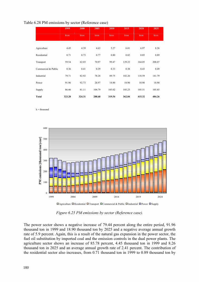
Table 6.28 PM emissions by sector (Reference case) 1999 2000 2005 2010 2015 2020 2025


Agriculture 4.45 4.39 4.63 5.27 6.01 6.97 8.26

Residential 0.71 0.73 0.77 0.80 0.82 0.85 0.89

Transport 59.54 62.03 70.97 99.47 129.22 164.05 208.07


Industrial 79.71 82.92 78.28 89.75 102.26 118.59 141.79

Power 91.96 92.73 28.97 18.90 18.90 18.90 18.90

Supply 86.46 81.11 104.79 105.02 105.25 105.51 105.85

Total 323.20 324.31 288.68 319.54 362.84 415.32 484.26

k = thousand

0

100

200

300

400

500

600

1999 2004 2009 2014 2019 2024

PM e

mis

sion

s [th

ousa

nd to

n/ye

ar]


Figure 6.25 PM emissions by sector (Reference case).

The power sector shows a negative increase of 79.44 percent along the entire period, 91.96 thousand ton in 1999 and 18.90 thousand ton by 2025 and a negative average annual growth rate of 5.9 percent. Again, this is a result of the natural gas expansion in the power sector, the fuel oil substitution by imported coal and the emission controls in the dual power plants. The agriculture sector shows an increase of 85.78 percent, 4.45 thousand ton in 1999 and 8.26 thousand ton in 2025 and an average annual growth rate of 2.41 percent. The contribution of the residential sector also increases, from 0.71 thousand ton in 1999 to 0.89 thousand ton by

180

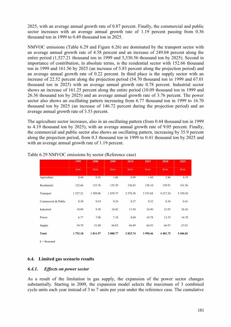
2025, with an average annual growth rate of 0.87 percent. Finally, the commercial and public sector increases with an average annual growth rate of 1.19 percent passing from 0.36 thousand ton in 1999 to 0.49 thousand ton in 2025.

NMVOC emissions (Table 6.29 and Figure 6.26) are dominated by the transport sector with an average annual growth rate of 4.58 percent and an increase of 249.04 percent along the entire period (1,527.21 thousand ton in 1999 and 5,330.56 thousand ton by 2025). Second in importance of contribution, in absolute terms, is the residential sector with 152.66 thousand ton in 1999 and 161.56 by 2025 (an increase of 5.83 percent along the projection period) and an average annual growth rate of 0.22 percent. In third place is the supply sector with an increase of 22.52 percent along the projection period (54.70 thousand ton in 1999 and 67.01 thousand ton in 2025) with an average annual growth rate 0.78 percent. Industrial sector shows an increase of 161.25 percent along the entire period (10.09 thousand ton in 1999 and 26.36 thousand ton by 2025) and an average annual growth rate of 3.76 percent. The power sector also shows an oscillating pattern increasing from 6.77 thousand ton in 1999 to 16.70 thousand ton by 2025 (an increase of 146.72 percent during the projection period) and an average annual growth rate of 3.53 percent.

The agriculture sector increases, also in an oscillating pattern (from 0.44 thousand ton in 1999 to 4.19 thousand ton by 2025), with an average annual growth rate of 9.05 percent. Finally, the commercial and public sector also shows an oscillating pattern, increasing by 35.9 percent along the projection period, from 0.3 thousand ton in 1999 to 0.41 thousand ton by 2025 and with an average annual growth rate of 1.19 percent.

Table 6.29 NMVOC emissions by sector (Reference case) 1999 2000 2005 2010 2015 2020 2025


Agriculture 0.44 0.56 1.06 0.99 1.69 2.86 4.19

Residential 152.66 153.76 155.29 156.83 158.10 159.91 161.56

Transport 1 527.21 1 589.06 1 839.73 2 578.58 3 335.68 4 217.24 5 330.56


Industrial 10.09 9.38 10.42 13.58 16.96 21.05 26.36

Power 6.77 7.08 7.18 8.60 10.78 13.35 16.70

Supply 54.70 51.80 66.85 66.89 66.93 66.97 67.01

Total 1 752.18 1 811.97 2 080.77 2 825.74 3 590.46 4 481.75 5 606.81

k = thousand

6.4. Limited gas scenario results

6.4.1. Effects on power sector

As a result of the limitation in gas supply, the expansion of the power sector changes substantially. Starting in 2009, the expansion model selects the maximum of 3 combined cycle units each year instead of 3 to 7 units per year under the reference case. The cumulative

181

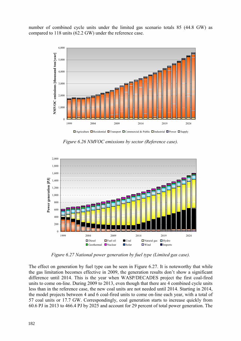
number of combined cycle units under the limited gas scenario totals 85 (44.8 GW) as compared to 118 units (62.2 GW) under the reference case.

0

1,000

2,000

3,000

4,000

5,000

6,000

1999 2004 2009 2014 2019 2024

NM

VO

C e

mis

sion

s [th

ousa

nd to

n/ye

ar]


Figure 6.26 NMVOC emissions by sector (Reference case).

0

200

400

600

800

1,000

1,200

1,400

1,600

1,800

2,000

1999 2004 2009 2014 2019 2024

Pow

er g

ener

atio

n [P

J]

Diesel Fuel oil Coal Natural gas HydroGeothermal Nuclear Solar Wind Imports

Figure 6.27 National power generation by fuel type (Limited gas case).

The effect on generation by fuel type can be seen in Figure 6.27. It is noteworthy that while the gas limitation becomes effective in 2009, the generation results don’t show a significant difference until 2014. This is the year when WASP/DECADES project the first coal-fired units to come on-line. During 2009 to 2013, even though that there are 4 combined cycle units less than in the reference case, the new coal units are not needed until 2014. Starting in 2014, the model projects between 4 and 6 coal-fired units to come on-line each year, with a total of 57 coal units or 17.7 GW. Correspondingly, coal generation starts to increase quickly from 60.6 PJ in 2013 to 466.4 PJ by 2025 and account for 29 percent of total power generation. The

182

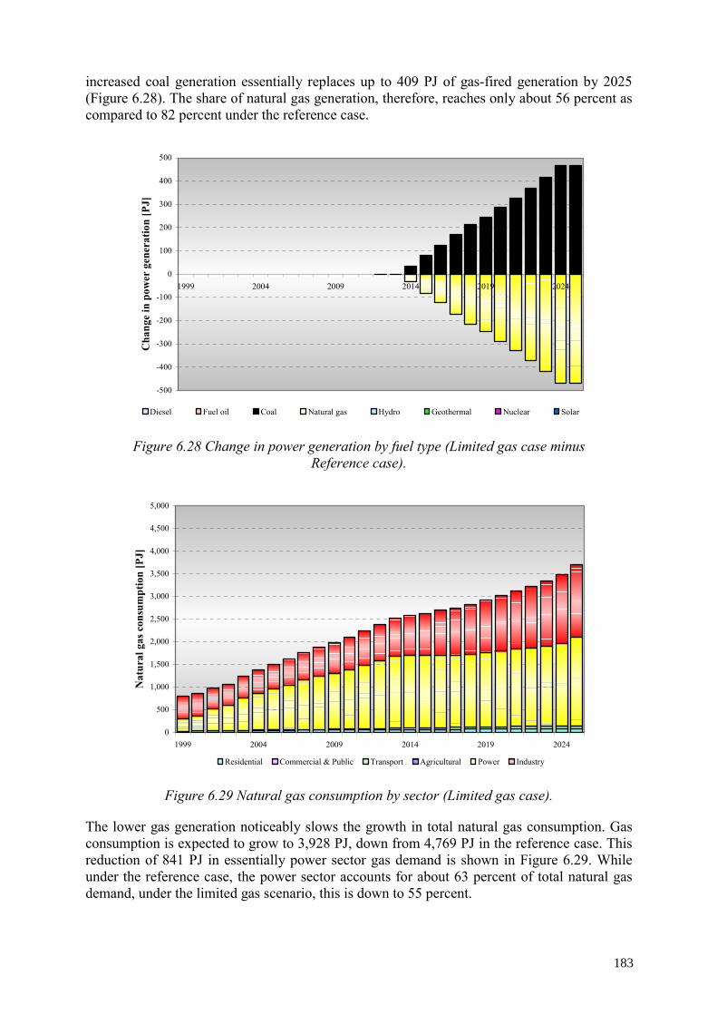
increased coal generation essentially replaces up to 409 PJ of gas-fired generation by 2025 (Figure 6.28). The share of natural gas generation, therefore, reaches only about 56 percent as compared to 82 percent under the reference case.

-500

-400

-300

-200

-100

0

100

200

300

400

500

1999 2004 2009 2014 2019 2024

Cha

nge

in p

ower

gen

erat

ion

[PJ]

Diesel Fuel oil Coal Natural gas Hydro Geothermal Nuclear Solar

Figure 6.28 Change in power generation by fuel type (Limited gas case minus Reference case).

0

500

1,000

1,500

2,000

2,500

3,000

3,500

4,000

4,500

5,000

1999 2004 2009 2014 2019 2024

Nat

ural

gas

con

sum

ptio

n [P

J]

Residential Commercial & Public Transport Agricultural Power Industry

Figure 6.29 Natural gas consumption by sector (Limited gas case).

The lower gas generation noticeably slows the growth in total natural gas consumption. Gas consumption is expected to grow to 3,928 PJ, down from 4,769 PJ in the reference case. This reduction of 841 PJ in essentially power sector gas demand is shown in Figure 6.29. While under the reference case, the power sector accounts for about 63 percent of total natural gas demand, under the limited gas scenario, this is down to 55 percent.

183

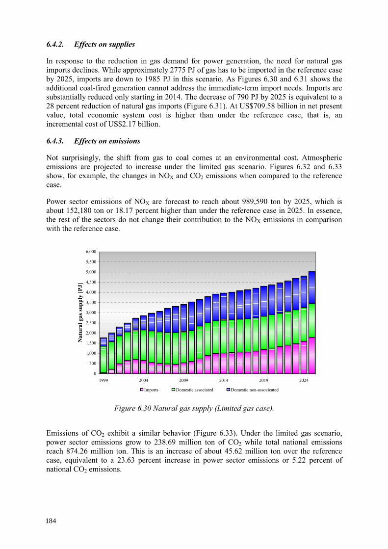
6.4.2. Effects on supplies

In response to the reduction in gas demand for power generation, the need for natural gas imports declines. While approximately 2775 PJ of gas has to be imported in the reference case by 2025, imports are down to 1985 PJ in this scenario. As Figures 6.30 and 6.31 shows the additional coal-fired generation cannot address the immediate-term import needs. Imports are substantially reduced only starting in 2014. The decrease of 790 PJ by 2025 is equivalent to a 28 percent reduction of natural gas imports (Figure 6.31). At US$709.58 billion in net present value, total economic system cost is higher than under the reference case, that is, an incremental cost of US$2.17 billion.

6.4.3. Effects on emissions

Not surprisingly, the shift from gas to coal comes at an environmental cost. Atmospheric emissions are projected to increase under the limited gas scenario. Figures 6.32 and 6.33 show, for example, the changes in NOX and CO2 emissions when compared to the reference case.

Power sector emissions of NOX are forecast to reach about 989,590 ton by 2025, which is about 152,180 ton or 18.17 percent higher than under the reference case in 2025. In essence, the rest of the sectors do not change their contribution to the NOX emissions in comparison with the reference case.

0

500

1,000

1,500

2,000

2,500

3,000

3,500

4,000

4,500

5,000

5,500

6,000

1999 2004 2009 2014 2019 2024

Nat

ural

gas

supp

ly [P

J]

Imports Domestic associated Domestic non-associcated

Figure 6.30 Natural gas supply (Limited gas case).

Emissions of CO2 exhibit a similar behavior (Figure 6.33). Under the limited gas scenario, power sector emissions grow to 238.69 million ton of CO2 while total national emissions reach 874.26 million ton. This is an increase of about 45.62 million ton over the reference case, equivalent to a 23.63 percent increase in power sector emissions or 5.22 percent of national CO2 emissions.

184

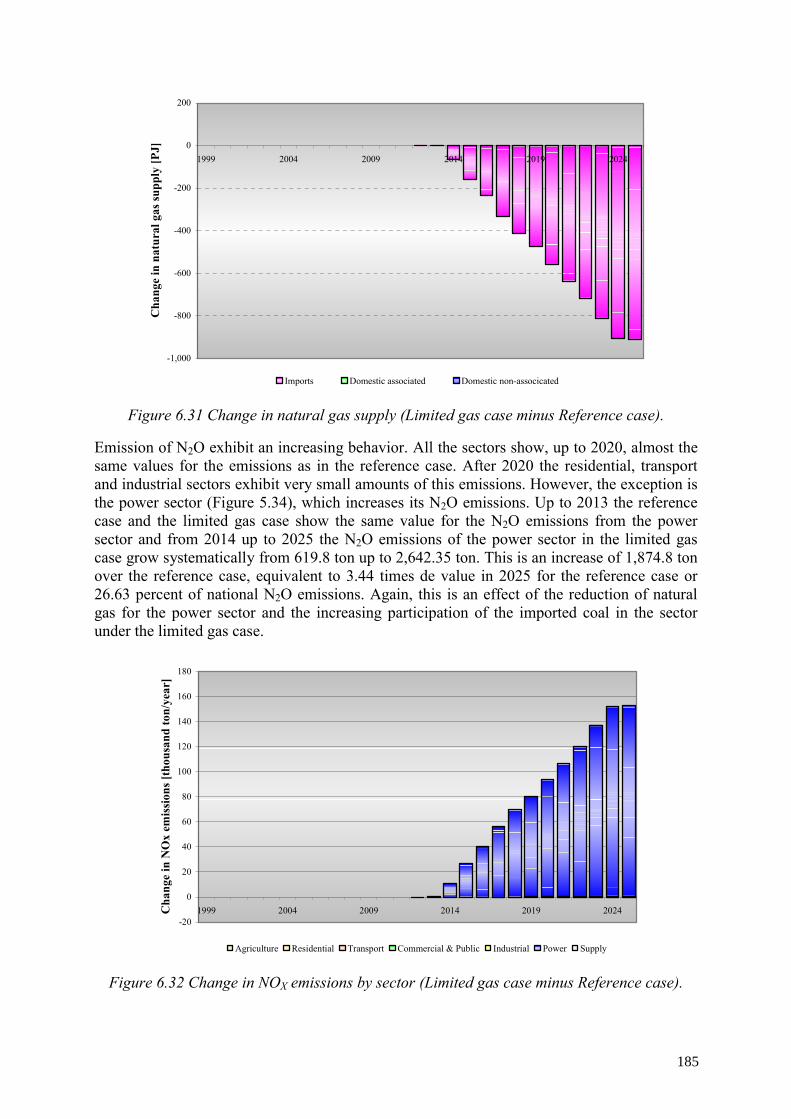
-1,000

-800

-600

-400

-200

0

200

1999 2004 2009 2014 2019 2024C

hang

e in

nat

ural

gas

supp

ly [P

J]

Imports Domestic associated Domestic non-associcated

Figure 6.31 Change in natural gas supply (Limited gas case minus Reference case).

Emission of N2O exhibit an increasing behavior. All the sectors show, up to 2020, almost the same values for the emissions as in the reference case. After 2020 the residential, transport and industrial sectors exhibit very small amounts of this emissions. However, the exception is the power sector (Figure 5.34), which increases its N2O emissions. Up to 2013 the reference case and the limited gas case show the same value for the N2O emissions from the power sector and from 2014 up to 2025 the N2O emissions of the power sector in the limited gas case grow systematically from 619.8 ton up to 2,642.35 ton. This is an increase of 1,874.8 ton over the reference case, equivalent to 3.44 times de value in 2025 for the reference case or 26.63 percent of national N2O emissions. Again, this is an effect of the reduction of natural gas for the power sector and the increasing participation of the imported coal in the sector under the limited gas case.

-20

0

20

40

60

80

100

120

140

160

180

1999 2004 2009 2014 2019 2024Cha

nge

in N

Ox

emis

sion

s [th

ousa

nd to

n/ye

ar]


Figure 6.32 Change in NOX emissions by sector (Limited gas case minus Reference case).

185

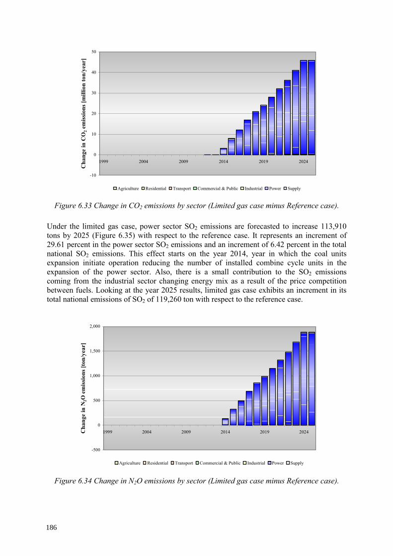
-10

0

10

20

30

40

50

1999 2004 2009 2014 2019 2024

Cha

nge

in C

O2 e

mis

sion

s [m

illio

n to

n/ye

ar]


Figure 6.33 Change in CO2 emissions by sector (Limited gas case minus Reference case).

Under the limited gas case, power sector SO2 emissions are forecasted to increase 113,910 tons by 2025 (Figure 6.35) with respect to the reference case. It represents an increment of 29.61 percent in the power sector SO2 emissions and an increment of 6.42 percent in the total national SO2 emissions. This effect starts on the year 2014, year in which the coal units expansion initiate operation reducing the number of installed combine cycle units in the expansion of the power sector. Also, there is a small contribution to the SO2 emissions coming from the industrial sector changing energy mix as a result of the price competition between fuels. Looking at the year 2025 results, limited gas case exhibits an increment in its total national emissions of SO2 of 119,260 ton with respect to the reference case.

-500

0

500

1,000

1,500

2,000

1999 2004 2009 2014 2019 2024Cha

nge

in N

2O e

mis

sion

s [to

n/ye

ar]


Figure 6.34 Change in N2O emissions by sector (Limited gas case minus Reference case).

186

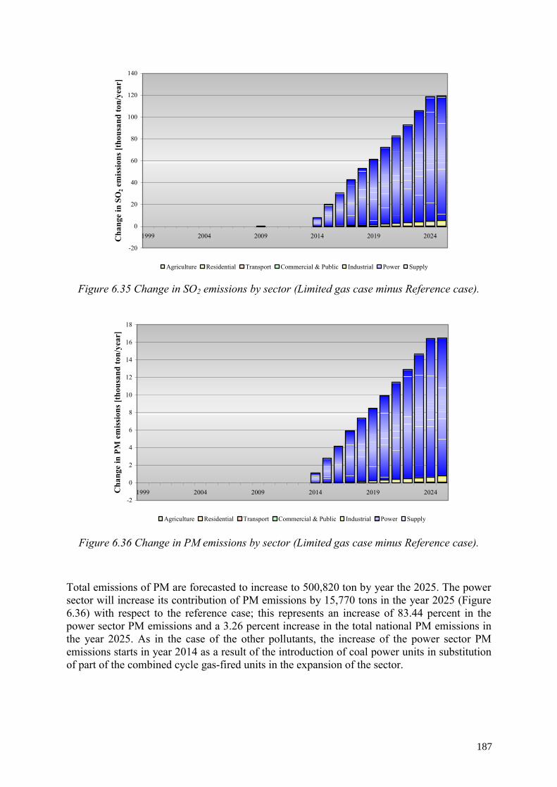
-20

0

20

40

60

80

100

120

140

1999 2004 2009 2014 2019 2024Cha

nge

in S

O2 e

mis

sion

s [th

ousa

nd to

n/ye

ar]


Figure 6.35 Change in SO2 emissions by sector (Limited gas case minus Reference case).

-2

0

2

4

6

8

10

12

14

16

18

1999 2004 2009 2014 2019 2024Cha

nge

in P

M e

mis

sion

s [th

ousa

nd to

n/ye

ar]


Figure 6.36 Change in PM emissions by sector (Limited gas case minus Reference case).

Total emissions of PM are forecasted to increase to 500,820 ton by year the 2025. The power sector will increase its contribution of PM emissions by 15,770 tons in the year 2025 (Figure 6.36) with respect to the reference case; this represents an increase of 83.44 percent in the power sector PM emissions and a 3.26 percent increase in the total national PM emissions in the year 2025. As in the case of the other pollutants, the increase of the power sector PM emissions starts in year 2014 as a result of the introduction of coal power units in substitution of part of the combined cycle gas-fired units in the expansion of the sector.

187

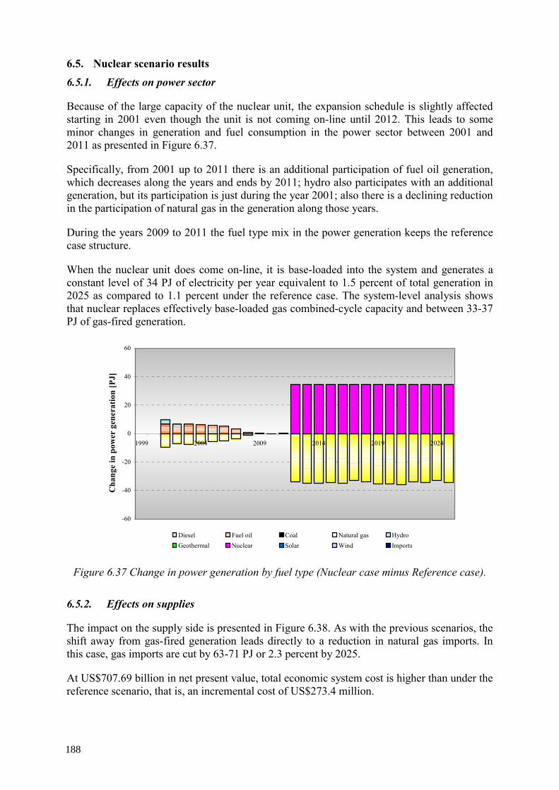
6.5. Nuclear scenario results


Because of the large capacity of the nuclear unit, the expansion schedule is slightly affected starting in 2001 even though the unit is not coming on-line until 2012. This leads to some minor changes in generation and fuel consumption in the power sector between 2001 and 2011 as presented in Figure 6.37.

Specifically, from 2001 up to 2011 there is an additional participation of fuel oil generation, which decreases along the years and ends by 2011; hydro also participates with an additional generation, but its participation is just during the year 2001; also there is a declining reduction in the participation of natural gas in the generation along those years.

During the years 2009 to 2011 the fuel type mix in the power generation keeps the reference case structure.

When the nuclear unit does come on-line, it is base-loaded into the system and generates a constant level of 34 PJ of electricity per year equivalent to 1.5 percent of total generation in 2025 as compared to 1.1 percent under the reference case. The system-level analysis shows that nuclear replaces effectively base-loaded gas combined-cycle capacity and between 33-37 PJ of gas-fired generation.

-60

-40

-20

0

20

40

60

1999 2004 2009 2014 2019 2024

Cha

nge

in p

ower

gen

erat

ion

[PJ]


Figure 6.37 Change in power generation by fuel type (Nuclear case minus Reference case).

6.5.2. Effects on supplies

The impact on the supply side is presented in Figure 6.38. As with the previous scenarios, the shift away from gas-fired generation leads directly to a reduction in natural gas imports. In this case, gas imports are cut by 63-71 PJ or 2.3 percent by 2025.

At US$707.69 billion in net present value, total economic system cost is higher than under the reference scenario, that is, an incremental cost of US$273.4 million.

188

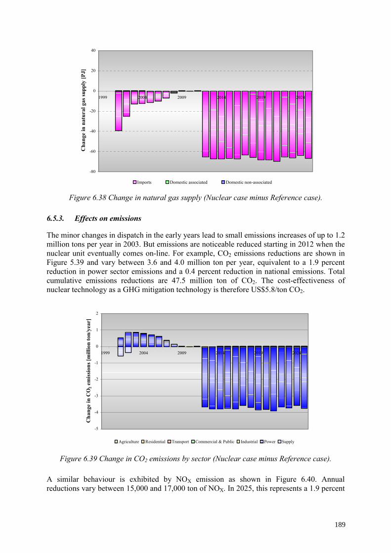
-80

-60

-40

-20

0

20

40

1999 2004 2009 2014 2019 2024

Cha

nge

in n

atur

al g

as su

pply

[PJ]

Imports Domestic associated Domestic non-associated Figure 6.38 Change in natural gas supply (Nuclear case minus Reference case).

6.5.3. Effects on emissions

The minor changes in dispatch in the early years lead to small emissions increases of up to 1.2 million tons per year in 2003. But emissions are noticeable reduced starting in 2012 when the nuclear unit eventually comes on-line. For example, CO2 emissions reductions are shown in Figure 5.39 and vary between 3.6 and 4.0 million ton per year, equivalent to a 1.9 percent reduction in power sector emissions and a 0.4 percent reduction in national emissions. Total cumulative emissions reductions are 47.5 million ton of CO2. The cost-effectiveness of nuclear technology as a GHG mitigation technology is therefore US$5.8/ton CO2.

-5

-4

-3

-2

-1

0

1

2

1999 2004 2009 2014 2019 2024

Cha

nge

in C

O2 e

mis

sion

s [m

illio

n to

n/ye

ar]


Figure 6.39 Change in CO2 emissions by sector (Nuclear case minus Reference case).

A similar behaviour is exhibited by NOX emission as shown in Figure 6.40. Annual reductions vary between 15,000 and 17,000 ton of NOX. In 2025, this represents a 1.9 percent

189

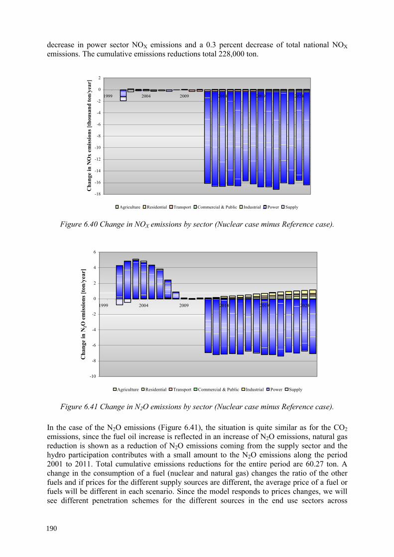
decrease in power sector NOX emissions and a 0.3 percent decrease of total national NOX emissions. The cumulative emissions reductions total 228,000 ton.

-18

-16

-14

-12

-10

-8

-6

-4

-2

0

2

1999 2004 2009 2014 2019 2024C

hang

e in

NO

x em

issi

ons [

thou

sand

ton/

year

]


Figure 6.40 Change in NOX emissions by sector (Nuclear case minus Reference case).

-10

-8

-6

-4

-2

0

2

4

6

1999 2004 2009 2014 2019 2024

Cha

nge

in N

2O e

mis

sion

s [to

n/ye

ar]


Figure 6.41 Change in N2O emissions by sector (Nuclear case minus Reference case).

In the case of the N2O emissions (Figure 6.41), the situation is quite similar as for the CO2 emissions, since the fuel oil increase is reflected in an increase of N2O emissions, natural gas reduction is shown as a reduction of N2O emissions coming from the supply sector and the hydro participation contributes with a small amount to the N2O emissions along the period 2001 to 2011. Total cumulative emissions reductions for the entire period are 60.27 ton. A change in the consumption of a fuel (nuclear and natural gas) changes the ratio of the other fuels and if prices for the different supply sources are different, the average price of a fuel or fuels will be different in each scenario. Since the model responds to prices changes, we will see different penetration schemes for the different sources in the end use sectors across

190

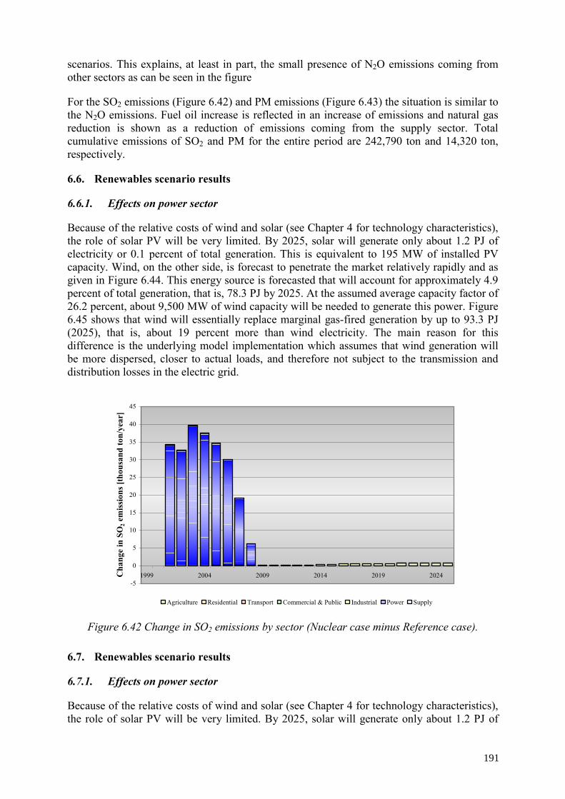
scenarios. This explains, at least in part, the small presence of N2O emissions coming from other sectors as can be seen in the figure

For the SO2 emissions (Figure 6.42) and PM emissions (Figure 6.43) the situation is similar to the N2O emissions. Fuel oil increase is reflected in an increase of emissions and natural gas reduction is shown as a reduction of emissions coming from the supply sector. Total cumulative emissions of SO2 and PM for the entire period are 242,790 ton and 14,320 ton, respectively.

6.6. Renewables scenario results


Because of the relative costs of wind and solar (see Chapter 4 for technology characteristics), the role of solar PV will be very limited. By 2025, solar will generate only about 1.2 PJ of electricity or 0.1 percent of total generation. This is equivalent to 195 MW of installed PV capacity. Wind, on the other side, is forecast to penetrate the market relatively rapidly and as given in Figure 6.44. This energy source is forecasted that will account for approximately 4.9 percent of total generation, that is, 78.3 PJ by 2025. At the assumed average capacity factor of 26.2 percent, about 9,500 MW of wind capacity will be needed to generate this power. Figure 6.45 shows that wind will essentially replace marginal gas-fired generation by up to 93.3 PJ (2025), that is, about 19 percent more than wind electricity. The main reason for this difference is the underlying model implementation which assumes that wind generation will be more dispersed, closer to actual loads, and therefore not subject to the transmission and distribution losses in the electric grid.

-5

0

5

10

15

20

25

30

35

40

45

1999 2004 2009 2014 2019 2024Cha

nge

in S

O2 e

mis

sion

s [th

ousa

nd to

n/ye

ar]


Figure 6.42 Change in SO2 emissions by sector (Nuclear case minus Reference case).

6.7. Renewables scenario results


Because of the relative costs of wind and solar (see Chapter 4 for technology characteristics), the role of solar PV will be very limited. By 2025, solar will generate only about 1.2 PJ of

191

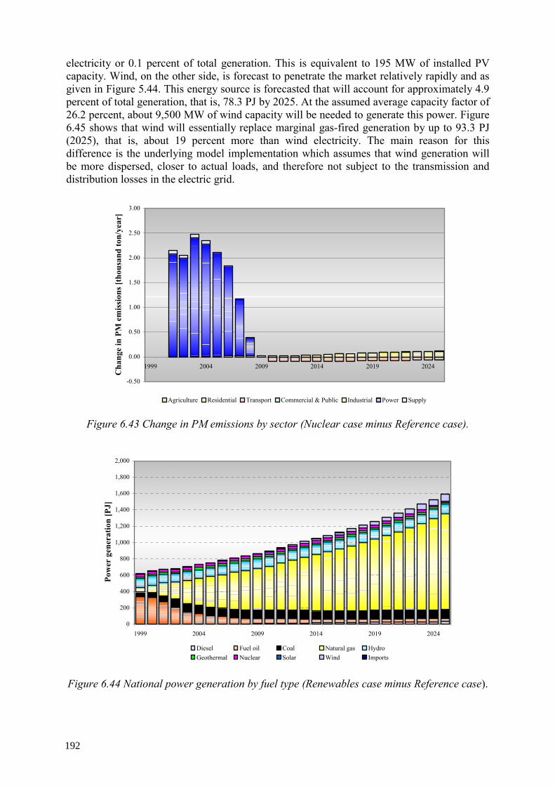
electricity or 0.1 percent of total generation. This is equivalent to 195 MW of installed PV capacity. Wind, on the other side, is forecast to penetrate the market relatively rapidly and as given in Figure 5.44. This energy source is forecasted that will account for approximately 4.9 percent of total generation, that is, 78.3 PJ by 2025. At the assumed average capacity factor of 26.2 percent, about 9,500 MW of wind capacity will be needed to generate this power. Figure 6.45 shows that wind will essentially replace marginal gas-fired generation by up to 93.3 PJ (2025), that is, about 19 percent more than wind electricity. The main reason for this difference is the underlying model implementation which assumes that wind generation will be more dispersed, closer to actual loads, and therefore not subject to the transmission and distribution losses in the electric grid.

-0.50

0.00

0.50

1.00

1.50

2.00

2.50

3.00

1999 2004 2009 2014 2019 2024

Cha

nge

in P

M e

mis

sion

s [th

ousa

nd to

n/ye

ar]


Figure 6.43 Change in PM emissions by sector (Nuclear case minus Reference case).

0

200

400

600

800

1,000

1,200

1,400

1,600

1,800

2,000

1999 2004 2009 2014 2019 2024

Pow

er g

ener

atio

n [P

J]


Figure 6.44 National power generation by fuel type (Renewables case minus Reference case).

192

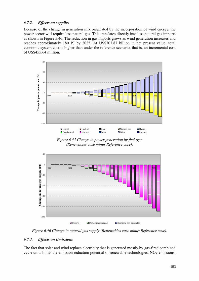
6.7.2. Effects on supplies Because of the change in generation mix originated by the incorporation of wind energy, the power sector will require less natural gas. This translates directly into less natural gas imports as shown in Figure 5.46. The reduction in gas imports grows as wind generation increases and reaches approximately 180 PJ by 2025. At US$707.87 billion in net present value, total economic system cost is higher than under the reference scenario, that is, an incremental cost of US$455.64 million.

-120

-80

-40

0

40

80

120

1999 2004 2009 2014 2019 2024

Cha

nge

in p

ower

gen

erat

ion

[PJ]


Figure 6.45 Change in power generation by fuel type (Renewables case minus Reference case).

-200

-160

-120

-80

-40

0

40

1999 2004 2009 2014 2019 2024

Cha

nge

in n

atur

al g

as su

pply

[PJ]

Imports Domestic associated Domestic non-associated Figure 6.46 Change in natural gas supply (Renewables case minus Reference case).

6.7.3. Effects on Emissions

The fact that solar and wind replace electricity that is generated mostly by gas-fired combined cycle units limits the emission reduction potential of renewable technologies. NOX emissions,

193

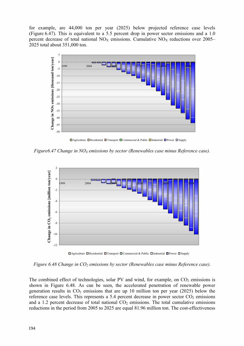
for example, are 44,000 ton per year (2025) below projected reference case levels (Figure 6.47). This is equivalent to a 5.5 percent drop in power sector emissions and a 1.0 percent decrease of total national NOX emissions. Cumulative NOX reductions over 2005–2025 total about 351,000 ton.

-50

-45

-40

-35

-30

-25

-20

-15

-10

-5

0

5

1999 2004 2009 2014 2019 2024

Cha

nge

in N

Ox

emis

sion

s [th

ousa

nd to

n/ye

ar]


Figure6.47 Change in NOX emissions by sector (Renewables case minus Reference case).

-12

-10

-8

-6

-4

-2

0

2

1999 2004 2009 2014 2019 2024

Cha

nge

in C

O2 e

mis

sion

s [m

illio

n to

n/ye

ar]


Figure 6.48 Change in CO2 emissions by sector (Renewables case minus Reference case).

The combined effect of technologies, solar PV and wind, for example, on CO2 emissions is shown in Figure 6.48. As can be seen, the accelerated penetration of renewable power generation results in CO2 emissions that are up 10 million ton per year (2025) below the reference case levels. This represents a 5.4 percent decrease in power sector CO2 emissions and a 1.2 percent decrease of total national CO2 emissions. The total cumulative emissions reductions in the period from 2005 to 2025 are equal 81.96 million ton. The cost-effectiveness

194

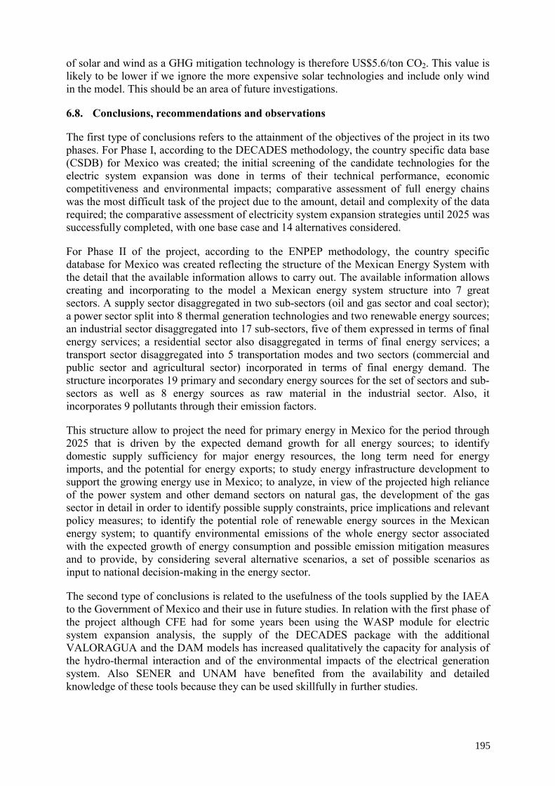
of solar and wind as a GHG mitigation technology is therefore US$5.6/ton CO2. This value is likely to be lower if we ignore the more expensive solar technologies and include only wind in the model. This should be an area of future investigations.

6.8. Conclusions, recommendations and observations

The first type of conclusions refers to the attainment of the objectives of the project in its two phases. For Phase I, according to the DECADES methodology, the country specific data base (CSDB) for Mexico was created; the initial screening of the candidate technologies for the electric system expansion was done in terms of their technical performance, economic competitiveness and environmental impacts; comparative assessment of full energy chains was the most difficult task of the project due to the amount, detail and complexity of the data required; the comparative assessment of electricity system expansion strategies until 2025 was successfully completed, with one base case and 14 alternatives considered.

For Phase II of the project, according to the ENPEP methodology, the country specific database for Mexico was created reflecting the structure of the Mexican Energy System with the detail that the available information allows to carry out. The available information allows creating and incorporating to the model a Mexican energy system structure into 7 great sectors. A supply sector disaggregated in two sub-sectors (oil and gas sector and coal sector); a power sector split into 8 thermal generation technologies and two renewable energy sources; an industrial sector disaggregated into 17 sub-sectors, five of them expressed in terms of final energy services; a residential sector also disaggregated in terms of final energy services; a transport sector disaggregated into 5 transportation modes and two sectors (commercial and public sector and agricultural sector) incorporated in terms of final energy demand. The structure incorporates 19 primary and secondary energy sources for the set of sectors and sub-sectors as well as 8 energy sources as raw material in the industrial sector. Also, it incorporates 9 pollutants through their emission factors.

This structure allow to project the need for primary energy in Mexico for the period through 2025 that is driven by the expected demand growth for all energy sources; to identify domestic supply sufficiency for major energy resources, the long term need for energy imports, and the potential for energy exports; to study energy infrastructure development to support the growing energy use in Mexico; to analyze, in view of the projected high reliance of the power system and other demand sectors on natural gas, the development of the gas sector in detail in order to identify possible supply constraints, price implications and relevant policy measures; to identify the potential role of renewable energy sources in the Mexican energy system; to quantify environmental emissions of the whole energy sector associated with the expected growth of energy consumption and possible emission mitigation measures and to provide, by considering several alternative scenarios, a set of possible scenarios as input to national decision-making in the energy sector.

The second type of conclusions is related to the usefulness of the tools supplied by the IAEA to the Government of Mexico and their use in future studies. In relation with the first phase of the project although CFE had for some years been using the WASP module for electric system expansion analysis, the supply of the DECADES package with the additional VALORAGUA and the DAM models has increased qualitatively the capacity for analysis of the hydro-thermal interaction and of the environmental impacts of the electrical generation system. Also SENER and UNAM have benefited from the availability and detailed knowledge of these tools because they can be used skillfully in further studies.

195

For the phase II of the project the tool supplied by the IAEA to the Government of Mexico was the ENPEP model developed by Argonne National Laboratory. This IAEA tool in conjunction with the energy demand model MODEMA developed at the Dirección General de Servicios de Cómputo Académico of UNAM allow to study the energy supply and demand implications incorporating the effect of energy prices and the competition between different energy sources.

The third type of conclusions refers to the synthetic analysis of the main results of energy projections for the entire Mexican energy system as for the study of the system level expansion of the power sector and the DAM program. In this respect, the basic expansion of the interconnected system would be based on natural gas-fired combined cycle units, with some gas turbines for peak demand hours. Nonetheless, the possibility of natural gas prices increases makes it desirable to consider some diversification using alternative technologies such as coal fired dual units, fuel oil units, and nuclear units. In such cases the total discounted costs can increase but a higher diversification is provided, the dependence on foreign fuel sources supply is reduced increasing the independence of this strategic sector. Moreover, some environmental benefits can be obtained as well, such as lower CO2, NOX, PM and SO2 emissions in the case of nuclear units and renewable energies.

The ENPEP methodology allows a detailed analysis of the effects of such an energy policy on the Mexican oil and gas industry as well as the effects on the energy supply and consumption of the rest of the economical activities. In addition allows studying and analyzing the environmental impacts of the energy supply and consumption activities.

The fourth type of conclusions to be derived from the study is the need for SENER, CFE and UNAM to analyze with much more detail the issue of economic, environmental, social and political impact of the diversification of the mix of technologies for the long term expansion of the electric system in Mexico as well as for the entire Mexican energy system. This conclusion arises from the vulnerability that exists in case of limitations in the supply of natural gas or in the increase of their prices.

In the context of diversification it can be recommended that SENER, CFE and UNAM study the possible economic and environmental benefits of incorporating more wind, solar and geothermal units as candidate technologies for the expansion of the electric system and alternative technologies in the other sectors of the Mexican energy system. The results of these studies could indicate the need to incorporate wind and solar technologies in the COPAR document of CFE as well as in the outlook of the electric sector published by SENER [5]. On the other hand, at the level of the integrated Mexican energy system the need for the study of the possible economic and environmental costs and benefits of incorporating new technologies for transportation, industrial process and final end uses in the different sector of the energy system.

For the four scenarios analyzed in the present study the specific and detailed conclusions, observations and recommendations are as follows:

6.8.1. Reference case

Under the selected GDP and population scenarios and unlimited natural gas case –reference case- the main conclusions, recommendations and observations are:

6.8.2. Energy

• Mexico will continue to rely heavily on fossil fuels for its energy trade and final energy consumption.

196

• Crude oil market share decrease from 68.2 percent in 1999 to 62.7 percent in 2025, as a consequence of the non-associated gas growth share in 11.9 percent in 2025 (compared with 4.5 percent in 1999) meanwhile associated gas decrease from 13.9 percent in 1999 to 12.8 percent in 2025. Non-associated gas average annual growth rate is the highest (5.2%) followed by coal (3.7%), crude oil (1.0%), geothermal (0.8%) and sugar cane bagasse (0.2%).

• Crude oil production increase, in millions of barrels per day, from 2.91 in 1999 to 3.49 in 2005, to 3.58 in 2010, to 3.65 in 2015, to 3.72 in 2020 and 3.78 in 2025. The projected production allow to satisfy the internal consumption (feedstock for the domestic refining system (1.35 million barrels per day in 1999 and 1.71 million barrels per day in 2025), including the programmed expansion of the refining capacity in the system, as well as the maquila mechanism along the entire period) plus the projected crude oil exports (1.55 million barrels per day in 1999 to 2.07 million barrels per day in 2025).

• In order to reduce the dependency on imported gasoline and increase gasoline exports refining capacity has to increase according to the following results: by 2006 domestic refining capacity increase to 1.715 million barrels per day, which will cover, in essence, the projected gasoline demand with a deficit of 27,000 barrels per day (this demand deficit could be covered through the maquila mechanism or through imports); after year 2008 and the rest of the projection period, once the completion of the reconfiguration program with a gasoline yielding of 39 percent, the total refining capacity increase, in millions of barrels per day, up to 1.94 by 2008, to 2.48 in 2015, 3.16 in 2020 and to 4.07 in 2025. Therefore, the accumulated increase capacity along the projection period is 2.36 million barrels per day. The elimination of the gasoline exports has the effect to reduce the additional capacity to 2.1 million barrels per day.

• Natural gas production and imports increase its participation in the total primary energy supply at an average annual growth rate of 4.8 percent along the entire period. Associated and non-associated gas production grow at an average annual growth rate of 1 and 5.18 percent, respectively, while natural gas imports grow at an average annual growth rate of 15.75 percent. To keep a proper balance between supply and consumption with an important participation of domestic production, starting 2010, it will be necessary to incorporate more non-associated gas fields to production. The market share of natural gas increases to 45.3 percent by 2025.

• In order to handle the natural gas production and the imports, natural gas infrastructure (production wells, gas pipelines, processing centers and distribution) will have to grow at an accelerated level.

• Natural gas will be the primary fuel of choice for power system expansion and generation leading to a near term and long term need for additional gas imports (or accelerated expansion of domestic production). Natural gas-fired generation share will increases from 8.09 to 78.94 percent.

• Fuel oil generation share decreases from 53.96 to 2.46 percent as a result of the fuel oil reduction policy in the country and the conversion of fuel oil based dual generation units to imported coal. Therefore, coal imports will increase from 3.36 million ton per year up to 7.99 million ton per year in 2002 and stay at the same level for the rest of the projection period.

197

• In absolute terms coal generation grows, however its share decreases from 9.82 to 6.61 percent.

• Diesel shows an increasing share from 0.66 to 2.02 percent as a result of its use in coal power generation plants and other sectors.

• Hydro and geothermal generation also grows in absolute terms, but their shares show a decreasing pattern.

• Nuclear generation decreases in absolute and percent wise terms due to no nuclear additions in the expansion scenario for the power sector and the retirement of the first unit of Laguna Verde nuclear power plant.

• Wind participates in the total generation with a very small amount and a decreasing share.

• Mexico will continue to rely heavily on refined oil products for its final energy consumption. Final energy consumption will increase at an average annual growth rate of 3.41 percent along the entire period.

• Mexico’s transport sector will continue to grow rapidly, at a 4.89 percent average annual growth rate, making transportation the largest final energy consumer in the country. Its market share grows from 38.39 percent in 1999 to 50.15 percent in 2025. Gasoline is expected to grow at an average annual growth rate of 4.99 percent, diesel at a 4.73 percent, kerosene at a 4.43 percent and LPG at a 3.25 percent. Fuel oil is expected to decrease at an average annual growth rate of 0.8 percent while natural gas increases its participation in road transport at an average annual growth rate of 24.27 percent. For natural gas penetration in the transport sector, it remains to see how real is this penetration rate under constraints on the availability of natural gas, transportation and distribution infrastructure.

• Industrial sector is the second highest final energy consumer with a 3.68 percent average annual growth rate; however its market share drops from 38.73 to 37.43 percent.

• Main energy consumption will be placed in the Cement, Iron and Steel, Chemical, and PEMEX Petrochemical sub sectors accounting for 46 percent of the total consumption.

• Natural gas and electricity will continue to be the most used fuels in the industrial sectors accounting for 65 percent.

• No changes of significance in the structure of the industrial energy consumption, other than the drastic reduction on fuel oil consumption, are to be expected.

• Nonetheless it is to be notice the impact of natural gas availability and price volatility in the energy bill of the industrial sector and the rest of the sectors.

• It is also to be noted the evolution of co-generation and self-generation in the industrial sector which are expected to grow 108 percent along the projection period; however the availability and price volatility of natural gas can cause adverse effects in these power generation activities.

• In the sugar sector biomass-based cogeneration, employing modern, efficient technology can be a cost-effective and a low greenhouse gas-emitting option but need significant investments to be developed.

198

• Final energy consumption in the agricultural sector increases at an average annual growth rate of 2.5 percent, but its market share falls from 2.9 to 2.08 percent. Clearly, if the needed re-activation of the sector and the current negotiations with the farmers have success, the impact on the energy consumption of the sector could be important.

• Commercial and public sectors energy consumption increases at an average annual growth rate of 2.22 percent; however its market share drops from 2.96 to 1.98 percent. Electricity becomes the main energy source with an average annual growth rate of 5.1 percent. The commercial sector has a good potential for electricity generated through renewable energies, both biomass and solar. Also, solar energy for water heating in substitution of fossil fuels has a good potential in the sector.

• Residential sector final energy consumption grows at an average annual growth rate of 1.01 percent loosing market share from 17.02 to 8.36 percent. LPG continues as the most important fuel in the sector in competition with natural gas. Firewood continues as the second energy source followed by electricity.

• As a result of the natural gas and fuel oil policies national CO2 (346.1 and 828.41 million ton in 1999 and 2025, respectively), NOX (1.52 and 4.61 million ton in 1999 and 2025, respectively), and PM (323.2 and 484.26 thousand ton in 1999 and 2025, respectively) emissions will increase while SO2 (2.35 and 1.78 million ton in 1999 and 2025, respectively) emissions are projected to decline.

6.8.3. Emissions

• By all means, the transport sector (shares of 31.08 and 44.73 percent in 1999 and 2025, respectively) becomes the most important contributor to the CO2, emissions followed by the power (shares of 28.37 and 23.31 percent in 1999 and 2025, respectively, showing the benefits of the energy policies in the sector), industrial (shares of 16.85 and 17.8 percent in 1999 and 2025, respectively) and supply (shares of 15.06 and 8.71 percent in 1999 and 2025, respectively) sectors. Residential, agriculture and commercial and public sectors contribute with shares of 8.64 in 1999 and 5.45 in 2025. Nevertheless, residential and commercial sectors are good candidates for the introduction of renewable energies, both biomass and solar for electricity generation as well as solar energy for water heating in substitution of fossil fuels.

• Also, transport sector is the most important contributor to the NOX emissions (shares of 66.84 percent in 1999 and 73.62 percent in 2025) followed by the power sector (18.59 percent in 1999 and 18.17 percent in 2025). The rest of the sectors contribute to these emissions with the 14.57 percent in 1999 and 8.21 percent in 2025. Clearly, actions aimed to reduce NOX emissions must have as its primary target the transport and power sectors, nevertheless existing technologies, rational energy use and fuel substitution measures can contribute to reduce the emissions in the other sectors.

• For PM emissions, also, the transport sector is the most important contributor (shares of 18.42 percent in 1999 and 42.97 percent in 2025) followed by the industrial sector (24.66 percent in 1999 and 29.28 percent in 2025). As a result of the energy policy in the power sector PM emission decrease from a share of 28.45 percent in 1999 to 3.89 percent in 2025. The supply sector reduces it share from 26.7 percent in 1999 to 21.86 in 2025, however, in absolute terms shows an increase in the PM emissions. The rest of the sectors show an increase in its share (1.71 percent in 1999 and 1.99 percent in 2025).

199

Finally, SO2 emissions show a decreasing pattern. The origin of this behavior is the energy policy in the power sector with shares of 72.9 percent in 1999 and 21.67 percent in 2025. However, part of this beneficial result in wiped out by the increase in the industrial sector (shares of 18.85 percent in 1999 and 60.19 in 2025), the increase in the supply sector (shares of 5.03 in 1999 and 8.62 in 2025), the increase in the transport sector (2.33 percent in 1999 and 7.38 in 2025). The rest of the sector also have increases and, as a set; represent participations of 0.9 percent in 1999 and 2.15 in 2025.

6.9. Alternative scenarios

6.9.1. Limited gas scenario

6.9.2. Energy

• If natural gas supply is limited, the power sector may shift to imported coal combustion for system expansion substantially decreasing the need for gas imports. However, this shift will come at an economic and environmental expense leading to significantly higher system costs and atmospheric emissions.

• Natural gas imports will keep, essentially, the same value as in the reference case, however, starting 2014 there will be a reduction in the natural gas imports of 5.87 percent with respect to the reference case and this difference will reach a 33.78 percent by 2025, also with respect to the reference case. Clearly, this will lower the pressure for the development of the needed infrastructure for production, transportation and distribution of natural gas; however, it will transfer this pressure to the development of the corresponding infrastructure for the reception, transportation and distribution of imported coal. According to the available information, current coal reception, transportation and distribution infrastructure allows for the handling of 4 million ton per year. Under this scenario this infrastructure will have to grow and be able to handle 9.5 million ton in 2014. After 2014, the coal-handling infrastructure will have to grow fast reaching a total handling capacity of 84.81 million ton of coal per year by 2025.

• Due to the natural gas supply limitation, the remaining sectors will adjust their energy mix, reducing the participation of natural gas and distributing the reduction between the remaining fuels in their energy mix. According to the model’s methodology, is expected that these distributions occur under the price competition for the different fuels within a given sector and between sectors. Since the current energy policy puts strong emphasis on the power sector, the natural gas supply limitation affects, directly to this sector, while for the remaining sectors the effect is less important.

6.9.3. Emissions

• Not surprisingly, the shift from natural gas to imported coal comes at an environmental cost. Atmospheric emissions are projected to increase under the limited gas scenario. Compared to the reference case, power sector CO2 emissions are forecast to reach about 238.69 million ton by 2025, which is about 45.62 million ton over or 23.63 percent higher than the reference case in 2025. Emissions of NOX exhibit a similar behavior under the limited gas scenario, they reach about 989,590 ton by 2025, which is about 152,180 ton or 18.17 percent higher than he reference case in 2025. The PM and SO2 emissions from the power sector are forecast to increase by 15,770 ton and 113,910 ton by 2025, respectively, also with respect to

200

the reference case. In essence, the remaining sectors show, relatively small changes in their contributions to the emissions with respect to the reference case.

6.10. Nuclear Scenario

6.10.1. Energy

• Nuclear power also replaces base-loaded gas-fired generation and thereby can lead to lower gas imports and lower emissions. Because of the large capacity of the nuclear unit, the expansion schedule is slightly affected starting in 2001 even though the unit is not coming on-line until 2012. This leads to some changes in generation and fuel consumption in the power sector between 2001 and 2011. Between 2001 and 2011 there is an additional participation of fuel oil generation, which decreases along the years and ends by 2011 and a reduction in the consumption of natural gas. When de nuclear unit does come on-line, it is base-loaded into the system and generates a constant level of 34 PJ of electricity per year equivalent to 1.5 percent of total generation in 2025 as compared to 1.1 percent under the reference case. The system-level analysis shows that nuclear replaces effectively base-loaded gas combined-cycle capacity and between 33-37 PJ of gas-fired generation. This represents a reduction in the imports of natural gas of 189.6 million cubic feet per day and an additional consumption of uranium dioxide of 31.31 ton per year. The remaining sectors show minor changes.

6.10.2. Emissions

• The changes in dispatch in the early years lead to small emissions increases of up to 1.2 million ton of CO2 per year in 2003. But emissions are noticeable reduced starting 2012 when the nuclear unit eventually comes on-line. CO2 emissions reductions vary between 3.6 and 4.0 million ton per year, equivalent to 1.9 percent reduction in power sector emissions and a 0.4 percent reduction in national emissions. Total cumulative reductions are 47.5 million ton of CO2 and the cost-effectiveness of nuclear technology as a GHG mitigation technology is therefore US$5.8 per ton of CO2.

• NOX emissions show a similar behavior and annual reductions vary between 15,000 and 17,000 ton of NOX. The cumulative emissions reductions total 228,000 ton.

• PM and SO2 emissions exhibit a similar behavior as CO2 and NOX emissions. Total cumulative emissions reductions of SO2 and PM emissions for the entire period are 242,790 and 14,320 ton, respectively.

• This calls for specific studies on the nuclear option. Special attention has to be paid to the total cost of the expansion scenarios including the internalization of the environmental externalities of the whole energy chain and looking for the total cost at which the nuclear option becomes competitive.

6.11. Renewables scenario

6.11.1. Energy

• Because of the relative costs of wind and solar, the role of solar PV will be very limited. By 2025, solar will generate only about 1.2 PJ of electricity or 0.1 percent of total generation. This is equivalent to 195 MW of installed PV capacity.

201

• Wind, on the other side, is forecast to penetrate the market relatively rapidly. This energy source is forecasted that will account approximately 4.9 percent of total generation that is 78.3 PJ by 2025. At the assumed capacity factor of 26.2 percent, about 9,500 MW of wind capacity will be needed to generate this power.

• Wind will essentially replace marginal gas-fired generation by up to 93.3 PJ in 2025, that is, about 19 percent more than wind electricity. The main reason for this difference is the underlying model implementation which assumes that wind generation will be more dispersed, closer to actual loads, and therefore not subject to the transmission and distribution losses of the electric grid.

• Due to the change in generation originated by the incorporation of wind energy, the power sector will require less natural gas and as a consequence less natural gas imports. The reduction in natural gas imports grows as wind generation increases and reaches approximately 178.31 PJ by 2025, which is equivalent to a reduction in the natural gas imports of 508.63 million cubic feet per day with respect to the reference case.

6.11.2. Emissions

• Renewables can contribute to GHG mitigation but their potential is somewhat limited as they mostly replace gas-fired generation.

• The combined effect of the accelerated penetration of renewable technologies in the power sector, solar PV and wind, results in CO2 emissions that are up to 10 million ton per year in 2025 below the reference case levels. This represents 5.4 percent decrease in the power sector CO2 emissions and a 1.2 percent decrease of total national CO2 emissions. The total cumulative emissions reductions in the period 2005 to 2025 are equal to 81.96 million ton.

• The cost-effectiveness of solar and wind a GHG mitigation technologies is therefore US$5.6 per ton of CO2. This value is likely to be lower if we ignore the more expensive solar technologies and include only wind in the model.

• This should be an area of future investigations in the power sector and other sectors as is the case of solar energy for water heating in substitution of fossil fuels in the residential and commercial sectors [4] as well as in the industrial sector.

• Also, it will be necessary to get and produce better information on the renewable energy costs and prices.

6.12. Additional comments and recommendations

It is known that in terms of the pure economic analysis e.g. considering the total cost of the expansion scenarios, the optimal solution is the Base Case or the decreased reliability scenarios, which is even more economic. But these decisions have the hidden costs of the environmental externalities (CO2, SOX, or other emissions), plus a possible security or diversification externality, which we have tried to understand and study. It is important to show the limitations of these scenarios in terms of environmental and social costs.

If the environmental externalities of the emissions are internalized, not only for the power plant but for the whole energy chain considered and the entire energy system, then the cleaner expansions (considering the forced nuclear expansion or increasing the reliability of the system), become potentially optimal and at the higher range cost of the CO2, the forced nuclear expansion solution becomes optimal. This is not a surprising result since the nuclear

202

unit is a zero emitter of greenhouse gases and if its operation starts in 2012, then a considerable amount of pollution is avoided. Using renewable resources such as wind power, which may have even better capital cost and construction periods, can produce the same effect. A study is under way to assess the introduction of such renewable resources, but was not included in this report.

On the other hand, if diversity is considered as an additional important component parameter, the options with higher diversity index become more competitive, and again some other options become optimal, for example the forced nuclear expansion and the limited combined cycle (LCC) scenarios are potentially optimal, being this last scenario optimal at the higher values of the diversity index. In both analysis the forced nuclear scenario (and equivalent forced renewable scenario), appear as good candidates for a reduction in environmental emissions and increasing the diversity of the system. Probably an optimal solution from the point of view of both emissions and diversity could be the introduction of a forced renewable scenario in the short term, and then a forced nuclear scenario in the longer term. This consideration remains as a matter of further study by SENER, CFE and UNAM.

As shown by the model results energy and energy services play and will continue to play a central role in the development of the Mexican energy system. The model results show how its needs for energy per unit GDP will increase steeply and how this growing demand for energy and energy services will have important consequences in emissions.

In general terms the model results reflects the mitigation strategy for greenhouse gases and other pollutants adopted recently by the Mexican government aiming to reduce fuel oil and LPG consumption and replace it by natural gas.

In light of the rapid growth of energy consumption in the industrial sector and other sectors, policies promoting energy efficiency and conservation should therefore continue to be an important component of energy policy. This energy policy and environmental management should shift towards a greater focus on structuring energy systems that promote sustainable development. Therefore, one of the key challenges for the Mexican energy system, today and in the future, will be the scaling up the activities of the different sectors in an economically, socially and environmentally sustainable way.

Energy efficiency measures include improved housekeeping procedures, maintenance, process control and automation, the replacement of outdated plant and equipment with the modern energy-efficient equivalent, and the recovery of embodied energy in recycled post-consumer wastes. This policy initiatives will have to be promoted in order to encourage the transfer and deployment of energy efficient technologies and/or measures which would then enable the system to deliver energy efficient products and services to consumers.

There is also a need to increase energy data availability and quality in the all the sectors. This is strictly necessary in order to improve the results of the model and the benefits of its use. Significant efforts are to be done in the characterization of the different conversion processes used in the industrial and other sectors. It is urgent to improve availability and reliability of the information related to energy efficiency, costs, final end uses, input/output ratios for different processes and final end uses, etc. This could be achieved by providing information, sources of information, accessibility to the information and a compromise of confidential and correct use of the provided information.

203

7. SPECIAL CHAPTER: “COMPARATIVE ASSESSMENT OF ENERGY SOURCES FOR ELECTRICITY SUPPLY UNTIL 2025”

7.1. Objectives and methodology of the study

This special chapter concentrates only in the discussion and results of the first phase of the national TC-project MEX/0/012: “Comparative Assessment of Energy Sources for Electricity Supply until 2025” that was carried out in the period 1999-2000. A study was conducted by the Mexican expert’s team under the coordination of SENER using DECADES tool that was provided by IAEA. Under this project, a comprehensive assessment of different energy supply options was conducted with environmental considerations in order to identify sustainable strategies to support the expected growth in electricity demand in Mexico. These results would provide in turn, the Mexican authorities with comprehensive information to make sound decisions regarding the expansion of the national electricity system.

7.1.1. Overview of the Mexican electric system

At present, the Mexican Public Power System produces electricity through the combustion of fossil fuels (coal, fuel oil, diesel and natural gas), through nuclear fuels, hydro resources and renewable energies (geothermal and wind). In 1999 the total primary energy consumption accounted for 6,280.49 PJ, of which Power Sector consumed 1,858.98 PJ producing 651.30 PJ of electricity (equivalent to an amount of brut power generation of 180.92 TW·h). Mexican power system rests, strongly, on fossil fuels and, as a consequence it becomes an important contributor to the global emissions of the country. In 1999 total capacity of the public power system was 35,666 MW, its composition by type of technology was discussed in Chapter 2, Section 2.4.2. Also, during 1999 total generation of the public power system was 180.92 TW·h. It is estimated that private producers contributed with an amount of 11,317 GW·h during 1999.

Country's actual energy policy privileges power generation through natural gas in detriment of fuel oil and nuclear. In this aspect, two independent prospective studies [3][4] indicate an important increase in the contribution to the power generation from natural gas and, also important, a reduction in fuel oil contribution. Natural gas increase is projected, mainly, through combined cycle generation technologies. Fuel oil reductions include the conversion to natural gas of eight fuel oil power plants (4,051 MW) and a dual power plant to imported coal (presently, Petacalco's power plant consumes fuel oil); all of them located in environmentally critical areas (Appendix I). Therefore, their conversion obeys to environmental and, in some cases, to economical reasons. However, due to the recent escalation of natural gas prices it becomes necessary to review this electric expansion policy, as well as the natural gas policy, and reevaluate the contribution of fuel oil, nuclear and other options.

Environmental impacts related to the operation of Electrical Energy Systems comprise the direct or indirect adverse effects and disadvantages phenomena that must be taken into consideration when discussing such a type of systems. Impacts are connected with the production, transmission, distribution and utilization of electrical energy, in both normal operation and other situations. In this sense, the environmental impacts related to the Electrical Energy Systems result from numerous complex phenomena and interactions, starting with the activities related to the exploration, mining, transportation, transformation of the fuels used in power generation up to the its utilization of the electricity for producing energy services.

205

Because of the complexity, generally is not possible to deal with all of the potential burdens, pathways and types of impacts in a single environmental impact study. The approach usually taken is to focus the environmental impact study on identifying and analyzing those, which appear, on a first review, to have the largest potential impacts in the specific situation. Owing to this, however, it is possible that some eventually important impacts will be overlooked. Also, this approach means that the potential environmental impacts of the different candidate energy sources and generation technologies are not fully evaluated. Therefore, resulting comparative assessment will not incorporate all aspects for the different options, which could lead to a “less than best” expansion strategy. In such a case, it will be necessary to review and monitor the performance of the strategy in order to determine whether any unforeseen damages are occurring, and to mitigate such effects.

The importance of energy sector planning and decision-making and, in particular, planning and decision making in the electrical sector has increased in the recent years due to its economical, social and environmental impacts. These two central activities, planning and decision making, must take into account a range of factors related to the entire fuel chain of the energy source, including their technical and economic performance as well as their impact on health and environment.

Cost, environment, options and strategies must be analyzed and compared in many different ways. Therefore, it is necessary to develop and apply tools, techniques and data for comparative assessment of different electricity generation options and strategies. In this sense, DECADES provides an enhancement, to some extent, of capabilities for comparative assessment of different electricity supply options and strategies in the process of planning and decision-making in the electricity sector.

The electricity planning perspective requires general characteristics data and analysis tools in order to understand the options available, as a function of the differences and tradeoffs between economic, health and environmental aspects of the different electric power technologies and alternative electricity supply policies. Therefore, this requires a detailed understanding of entire electric power system, the capacity growth that has to meet in the future, data on the fuel options and plant candidates for meeting the capacity expansion requirements, methods for the calculation of health impacts and environment related emissions and burdens from the cost-optimized expansion strategies. Also, the analysis is by nature highly specific and requires detailed data on the project costs, emissions and other burdens resulting from the plant construction and operation.

7.1.2. Objectives

The main study objectives are:

• To develop a Country Specific Data Base (CSDB) including technical, economic, and environmental parameters of alternative electricity generation technologies and their full energy chains; and,

• To study alternatives for the expansion of the Mexican generating system until 2025 at four analytical levels:

• Plant-level analysis;

• Chain-level analysis;

• System-level analysis; and,

• Decision-making analysis.

206

7.1.3. Methodology

The following methodological steps have been implemented in the study:

• Identify all possible fuels in the country (imported fuel included) in order to create the fuel inventory and implement them in CSDB. For each fuel (gas, oil, coal and nuclear) the potential resource and its availability for future plans are considered. The database involves the source, type and subtype of fuel and it contains economic, technical characteristics and environmental factors.

• Establish the existing electricity generation technologies (thermal and hydro plants) and consider candidate technologies. Some technologies to be considered are combined cycle based on natural gas; dual power plants based on coal with desulphurization, gas turbine, and nuclear power plants (ABWR) and a list of hydro power plants as candidates.

• Establish the auxiliary inputs for every step in the chain, e.g. self-consumption in its process (electricity, fuel, heat and mechanical power).

• Link the determined technologies for existing and candidates plants with the fuels to be considered according to the regional availability.

• In order to select the power generation plants considered as expansion alternatives, the screening curves for each technology will be prepared with the objective to determine which of these plants are more attractive.

• Define the chain boundaries (within the country boundaries) by energy chain (e.g. gaseous fuel, liquid fuel, solid fuel, nuclear, hydro and geothermal) and by steps in the energy chain (e.g. mining, transportation, preparation, electricity generation).

• Establish allocation criteria for steps in the energy chain with multiple inputs/outputs such as refineries and drilling sites. Review the direct and indirect emission factors for main air pollutants. Assess the emissions of radionuclides in air and water from the nuclear energy chain. Estimate chain specific emissions (e.g. CH4 emissions associated with the hydro reservoirs). Calculate levelized full chain electricity generation costs. The calculation performed will take into consideration different chain specific aspects, such as transportation distance for fuels.

• Assess and compare the full energy chains of the country (gaseous fuel, liquid fuel, solid fuel, nuclear, hydro and geothermal) in terms of their technical performances, economic characteristics and environmental parameters and considering their steps: mining, transportation, preparation, electricity generation, and waste disposal. Compare the levelized full chain electricity generation costs and air pollutants and air emissions of radionuclides.

• Perform analysis considering all possible supply sources in the country and select the expansion scenarios to be studied in order to obtain different alternative expansion plans which take in consideration technical, economic and system reliability factors. These alternative expansion plans will be assumed in order to provide information to the decision makers and obtain a robust plan.

• Define different scenarios in order to be able of study the impact of higher demand growth, nuclear option, escalation of fossil fuel prices, limitations of new gas-fires units, discount rate and changes of the reliability on the power system expansion.

207

• Prepare information about fixed system and candidate technologies aggregating in the database technical and economic data.

• Prepare additional information, which is necessary to perform the system analysis (demand, economic parameters, operation constrains and reliability criteria).

• Carry out the system analysis using DECPAC; the analytical software of DECADES, in order to obtain the optimal solution of different expansion alternative plans incorporating Valor Agua model results interactively.

• Select a number of alternatives over which we can take a decision about. Define criteria, such as CO2, SOx, NOx, particulates emissions and the criterion for the diversity of the system as represented by the Stirling Index, and determine weights to study/evaluate the scenarios selected.

• Conduct decision-making analysis of the selected alternatives using the DAM (Decision Analysis Module) of the DECADES package with all gathered data in order to obtain the relevant conclusions to be given to the decision makers.

7.1.4. Modeling approach

As described earlier, DECADES is the modeling tool that was used in this part of the study. It is an integrated software package developed to provide senior analysts and energy experts with an easy to use tool for carrying out decision support studies for the power sector. Briefly, these tools consist of:

• Several databases providing a comprehensive, harmonized set of technical, economic and environmental data for energy chains that use fossil fuel, nuclear power and renewable energy sources for electricity generation;

• A data management system which provides user friendly access to the DECADES databases;

• An analytical software designed to access the information stored in the databases for analysis of costs and environmental burdens at the power plant, full energy chain and electric system levels; and,

• A decision analysis tool. The DECADES tools are RTDB, CSDB, HEIES, and DECPAC. They consist of databases and analytical programs, which can be used for national, regional and international studies in order to evaluate trade-offs between technical, economic and environmental aspects of different electricity generation technologies, chains, and systems. For a detailed description of the DECADES methodology see section 3.3 of the Summary of the present report.

7.2. Chain-level analysis

As was mentioned in Section 7.1.2, the study of the alternatives for the expansion of the Mexican generating system was carried out at four analytical levels: plant-level analysis, chain-level analysis, system-level analysis and decision-making analysis. Plant-level analysis provides to the user with a preliminary screening of different electricity generation options, emission factors for main air pollutants are estimated based on fuel characteristics and power plant performances. On the other hand, System-level analysis also provides a screening of the generation system expansion strategies and the conduction of comprehensive studies to develop mixes of energy chains, which meet electricity demand for a country or region. The environmental residuals are estimated taking into account the full energy chains composing

208

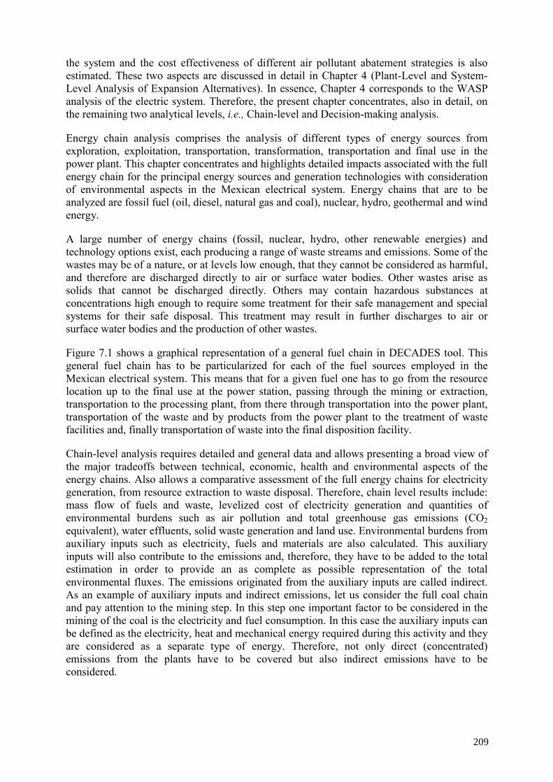
the system and the cost effectiveness of different air pollutant abatement strategies is also estimated. These two aspects are discussed in detail in Chapter 4 (Plant-Level and System-Level Analysis of Expansion Alternatives). In essence, Chapter 4 corresponds to the WASP analysis of the electric system. Therefore, the present chapter concentrates, also in detail, on the remaining two analytical levels, i.e., Chain-level and Decision-making analysis.

Energy chain analysis comprises the analysis of different types of energy sources from exploration, exploitation, transportation, transformation, transportation and final use in the power plant. This chapter concentrates and highlights detailed impacts associated with the full energy chain for the principal energy sources and generation technologies with consideration of environmental aspects in the Mexican electrical system. Energy chains that are to be analyzed are fossil fuel (oil, diesel, natural gas and coal), nuclear, hydro, geothermal and wind energy.

A large number of energy chains (fossil, nuclear, hydro, other renewable energies) and technology options exist, each producing a range of waste streams and emissions. Some of the wastes may be of a nature, or at levels low enough, that they cannot be considered as harmful, and therefore are discharged directly to air or surface water bodies. Other wastes arise as solids that cannot be discharged directly. Others may contain hazardous substances at concentrations high enough to require some treatment for their safe management and special systems for their safe disposal. This treatment may result in further discharges to air or surface water bodies and the production of other wastes.

Figure 7.1 shows a graphical representation of a general fuel chain in DECADES tool. This general fuel chain has to be particularized for each of the fuel sources employed in the Mexican electrical system. This means that for a given fuel one has to go from the resource location up to the final use at the power station, passing through the mining or extraction, transportation to the processing plant, from there through transportation into the power plant, transportation of the waste and by products from the power plant to the treatment of waste facilities and, finally transportation of waste into the final disposition facility.

Chain-level analysis requires detailed and general data and allows presenting a broad view of the major tradeoffs between technical, economic, health and environmental aspects of the energy chains. Also allows a comparative assessment of the full energy chains for electricity generation, from resource extraction to waste disposal. Therefore, chain level results include: mass flow of fuels and waste, levelized cost of electricity generation and quantities of environmental burdens such as air pollution and total greenhouse gas emissions (CO2 equivalent), water effluents, solid waste generation and land use. Environmental burdens from auxiliary inputs such as electricity, fuels and materials are also calculated. This auxiliary inputs will also contribute to the emissions and, therefore, they have to be added to the total estimation in order to provide an as complete as possible representation of the total environmental fluxes. The emissions originated from the auxiliary inputs are called indirect. As an example of auxiliary inputs and indirect emissions, let us consider the full coal chain and pay attention to the mining step. In this step one important factor to be considered in the mining of the coal is the electricity and fuel consumption. In this case the auxiliary inputs can be defined as the electricity, heat and mechanical energy required during this activity and they are considered as a separate type of energy. Therefore, not only direct (concentrated) emissions from the plants have to be covered but also indirect emissions have to be considered.

209

Energy fuel

Mining, fuel extraction

Fuel processing

Electricity generation

Fueltransportation

Transport of fuel processed

Transport of waste

Waste treatment

Transport of waste

Reprocessing of spent fuel

Transport of waste

Waste disposal

Transport of waste fuel and

by products

Transport of spent fuel

Transportation of reprocessed fuel

Electricity distribution

Level I

Level II

Level III

Level IV

Level V

Level VI

Level VIII

Level IX

Level X

Level X

Energy fuelEnergy fuel

Mining, fuel extraction

Fuel processing


Fueltransportation



Transport of waste

Transport of waste

Waste treatment

Transport of waste

Transport of waste

Reprocessing of spent fuel

Transport of waste

Transport of waste

Waste disposal


by products


by products





Electricity distributionElectricity

distribution

Level I

Level II

Level III

Level IV

Level V

Level VI

Level VIII

Level IX

Level X

Level X

Figure 7.1 Graphical representation of a generalized fuel chain.

7.2.1. Oil chain

Fuel oil and diesel are derived products from the crude oil. In the case of Mexico oil resources are located onshore and offshore. At present most of the oil production comes from the marine oil fields, located in the Gulf of Mexico. Most of the present production of oil it is associated with natural gas. Fuel oil and diesel, two by-products of the petroleum industry, are used as boiler fuels in thermal plants for electricity production, but they have other energy applications also. Therefore, it is necessary to consider the full energy chain. The impacts from the oil chain for electricity generation are associated with the overall activities for the oil exploration, production, processing and transportation.

The specific chain we use for this case is shown in detail in Figure 7.2. Additionally, the figure shows the associated auxiliary levels for each of the primary level or steps. The discussion will be carried out step-by-step indicating the data and main assumptions we made in the preparation of the input for the chains. Each one of the auxiliary levels in the figure is connected with one and only one step. The auxiliaries can be diesel, electricity, mechanical energy, etc

For a general discussion of the crude oil and gas production, processing, transportation and their environmental impacts see Appendix IV of the present report. For the oil and gas chains, we will refer the discussion to the levels or steps shown in Figure 6.2 and our analysis will be carried out step-by-step along the specific chain.

210

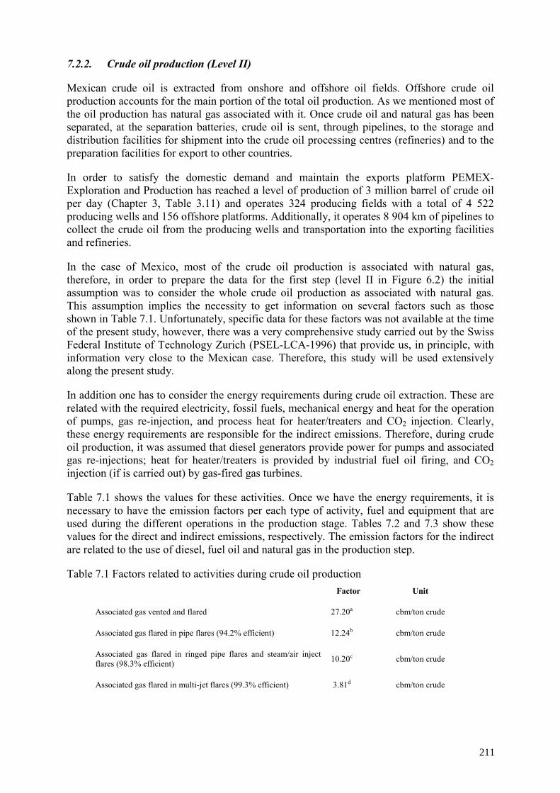
7.2.2. Crude oil production (Level II)

Mexican crude oil is extracted from onshore and offshore oil fields. Offshore crude oil production accounts for the main portion of the total oil production. As we mentioned most of the oil production has natural gas associated with it. Once crude oil and natural gas has been separated, at the separation batteries, crude oil is sent, through pipelines, to the storage and distribution facilities for shipment into the crude oil processing centres (refineries) and to the preparation facilities for export to other countries.

In order to satisfy the domestic demand and maintain the exports platform PEMEX-Exploration and Production has reached a level of production of 3 million barrel of crude oil per day (Chapter 3, Table 3.11) and operates 324 producing fields with a total of 4 522 producing wells and 156 offshore platforms. Additionally, it operates 8 904 km of pipelines to collect the crude oil from the producing wells and transportation into the exporting facilities and refineries.

In the case of Mexico, most of the crude oil production is associated with natural gas, therefore, in order to prepare the data for the first step (level II in Figure 6.2) the initial assumption was to consider the whole crude oil production as associated with natural gas. This assumption implies the necessity to get information on several factors such as those shown in Table 7.1. Unfortunately, specific data for these factors was not available at the time of the present study, however, there was a very comprehensive study carried out by the Swiss Federal Institute of Technology Zurich (PSEL-LCA-1996) that provide us, in principle, with information very close to the Mexican case. Therefore, this study will be used extensively along the present study.

In addition one has to consider the energy requirements during crude oil extraction. These are related with the required electricity, fossil fuels, mechanical energy and heat for the operation of pumps, gas re-injection, and process heat for heater/treaters and CO2 injection. Clearly, these energy requirements are responsible for the indirect emissions. Therefore, during crude oil production, it was assumed that diesel generators provide power for pumps and associated gas re-injections; heat for heater/treaters is provided by industrial fuel oil firing, and CO2 injection (if is carried out) by gas-fired gas turbines.

Table 7.1 shows the values for these activities. Once we have the energy requirements, it is necessary to have the emission factors per each type of activity, fuel and equipment that are used during the different operations in the production stage. Tables 7.2 and 7.3 show these values for the direct and indirect emissions, respectively. The emission factors for the indirect are related to the use of diesel, fuel oil and natural gas in the production step.

Table 7.1 Factors related to activities during crude oil production Factor Unit

Associated gas vented and flared 27.20a cbm/ton crude

Associated gas flared in pipe flares (94.2% efficient) 12.24b cbm/ton crude

Associated gas flared in ringed pipe flares and steam/air inject flares (98.3% efficient) 10.20c cbm/ton crude

Associated gas flared in multi-jet flares (99.3% efficient) 3.81d cbm/ton crude

211

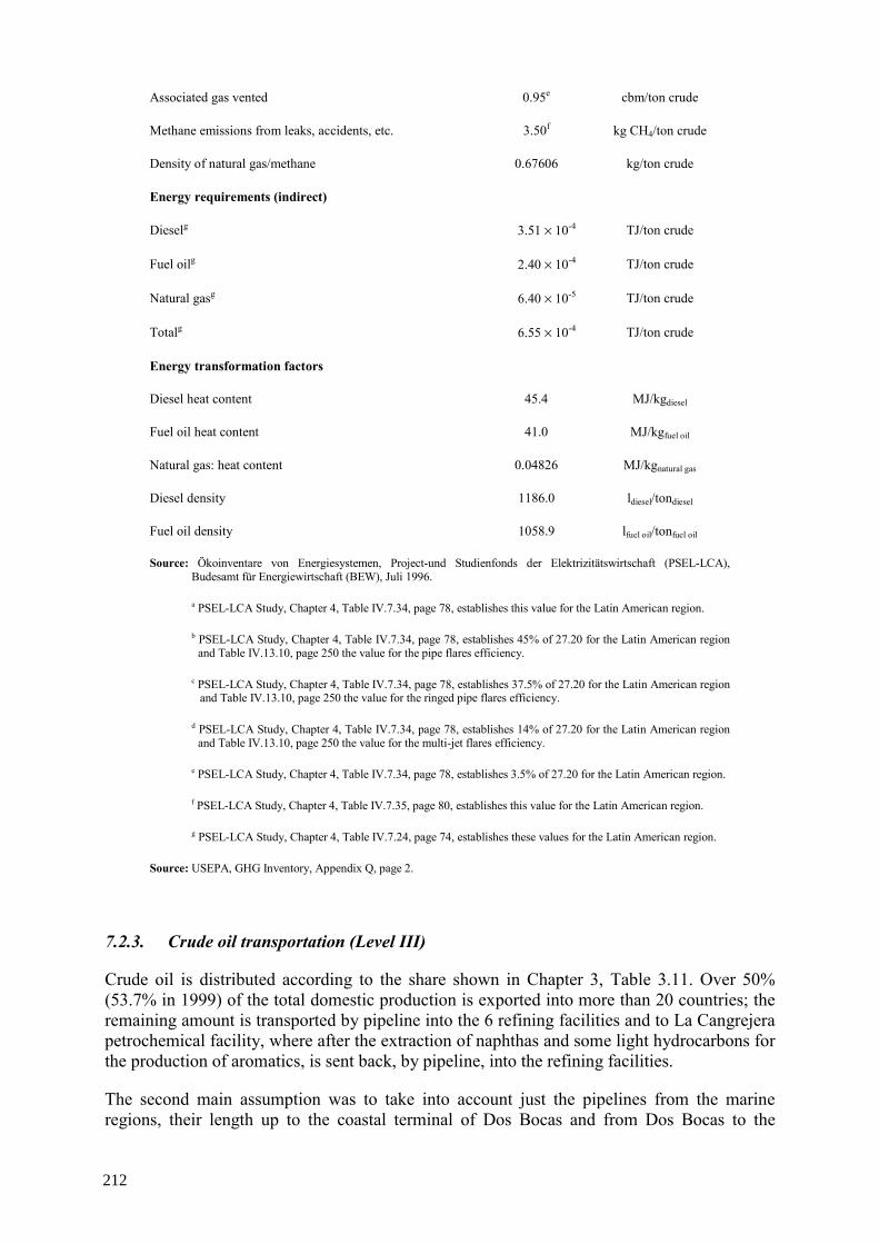
Associated gas vented 0.95e cbm/ton crude

Methane emissions from leaks, accidents, etc. 3.50f kg CH4/ton crude

Density of natural gas/methane 0.67606 kg/ton crude

Energy requirements (indirect)

Dieselg 3.51 × 10-4 TJ/ton crude

Fuel oilg 2.40 × 10-4 TJ/ton crude

Natural gasg 6.40 × 10-5 TJ/ton crude

Totalg 6.55 × 10-4 TJ/ton crude

Energy transformation factors

Diesel heat content 45.4 MJ/kgdiesel

Fuel oil heat content 41.0 MJ/kgfuel oil

Natural gas: heat content 0.04826 MJ/kgnatural gas

Diesel density 1186.0 ldiesel/tondiesel

Fuel oil density 1058.9 lfuel oil/tonfuel oil

Source: Ökoinventare von Energiesystemen, Project-und Studienfonds der Elektrizitätswirtschaft (PSEL-LCA), Budesamt für Energiewirtschaft (BEW), Juli 1996.

a PSEL-LCA Study, Chapter 4, Table IV.7.34, page 78, establishes this value for the Latin American region.

b PSEL-LCA Study, Chapter 4, Table IV.7.34, page 78, establishes 45% of 27.20 for the Latin American region and Table IV.13.10, page 250 the value for the pipe flares efficiency.

c PSEL-LCA Study, Chapter 4, Table IV.7.34, page 78, establishes 37.5% of 27.20 for the Latin American region and Table IV.13.10, page 250 the value for the ringed pipe flares efficiency.

d PSEL-LCA Study, Chapter 4, Table IV.7.34, page 78, establishes 14% of 27.20 for the Latin American region and Table IV.13.10, page 250 the value for the multi-jet flares efficiency.

e PSEL-LCA Study, Chapter 4, Table IV.7.34, page 78, establishes 3.5% of 27.20 for the Latin American region.

f PSEL-LCA Study, Chapter 4, Table IV.7.35, page 80, establishes this value for the Latin American region.

g PSEL-LCA Study, Chapter 4, Table IV.7.24, page 74, establishes these values for the Latin American region.

Source: USEPA, GHG Inventory, Appendix Q, page 2.

7.2.3. Crude oil transportation (Level III)

Crude oil is distributed according to the share shown in Chapter 3, Table 3.11. Over 50% (53.7% in 1999) of the total domestic production is exported into more than 20 countries; the remaining amount is transported by pipeline into the 6 refining facilities and to La Cangrejera petrochemical facility, where after the extraction of naphthas and some light hydrocarbons for the production of aromatics, is sent back, by pipeline, into the refining facilities.

The second main assumption was to take into account just the pipelines from the marine regions, their length up to the coastal terminal of Dos Bocas and from Dos Bocas to the

212

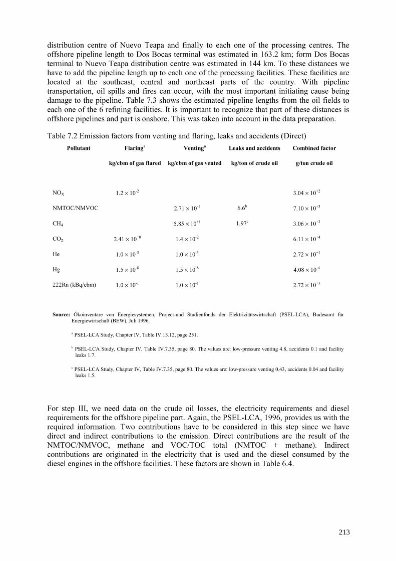
distribution centre of Nuevo Teapa and finally to each one of the processing centres. The offshore pipeline length to Dos Bocas terminal was estimated in 163.2 km; form Dos Bocas terminal to Nuevo Teapa distribution centre was estimated in 144 km. To these distances we have to add the pipeline length up to each one of the processing facilities. These facilities are located at the southeast, central and northeast parts of the country. With pipeline transportation, oil spills and fires can occur, with the most important initiating cause being damage to the pipeline. Table 7.3 shows the estimated pipeline lengths from the oil fields to each one of the 6 refining facilities. It is important to recognize that part of these distances is offshore pipelines and part is onshore. This was taken into account in the data preparation.

Table 7.2 Emission factors from venting and flaring, leaks and accidents (Direct) Pollutant Flaringa Ventinga Leaks and accidents Combined factor

kg/cbm of gas flared kg/cbm of gas vented kg/ton of crude oil g/ton crude oil

NOX 1.2 × 10-2 3.04 × 10+2

NMTOC/NMVOC 2.71 × 10-1 6.6b 7.10 × 10+3

CH4 5.85 × 10+1 1.97c 3.06 × 10+3

CO2 2.41 × 10+0 1.4 × 10-2 6.11 × 10+4

He 1.0 × 10-3 1.0 × 10-3 2.72 × 10+1

Hg 1.5 × 10-8 1.5 × 10-8 4.08 × 10-4

222Rn (kBq/cbm) 1.0 × 10-1 1.0 × 10-1 2.72 × 10+3


a PSEL-LCA Study, Chapter IV, Table IV.13.12, page 251.

b PSEL-LCA Study, Chapter IV, Table IV.7.35, page 80. The values are: low-pressure venting 4.8, accidents 0.1 and facility leaks 1.7.

c PSEL-LCA Study, Chapter IV, Table IV.7.35, page 80. The values are: low-pressure venting 0.43, accidents 0.04 and facility leaks 1.5.

For step III, we need data on the crude oil losses, the electricity requirements and diesel requirements for the offshore pipeline part. Again, the PSEL-LCA, 1996, provides us with the required information. Two contributions have to be considered in this step since we have direct and indirect contributions to the emission. Direct contributions are the result of the NMTOC/NMVOC, methane and VOC/TOC total (NMTOC + methane). Indirect contributions are originated in the electricity that is used and the diesel consumed by the diesel engines in the offshore facilities. These factors are shown in Table 6.4.

213

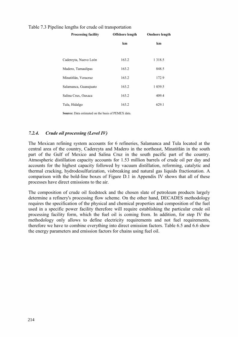
Table 7.3 Pipeline lengths for crude oil transportation Processing facility Offshore length Onshore length

km km

Cadereyta, Nuevo León 163.2 1 318.5

Madero, Tamaulipas 163.2 848.5

Minatitlán, Veracruz 163.2 172.9

Salamanca, Guanajuato 163.2 1 039.5

Salina Crux, Oaxaca 163.2 409.4

Tula, Hidalgo 163.2 629.1

Source: Data estimated on the basis of PEMEX data.

7.2.4. Crude oil processing (Level IV)

The Mexican refining system accounts for 6 refineries, Salamanca and Tula located at the central area of the country, Cadereyta and Madero in the northeast, Minatitlán in the south part of the Gulf of Mexico and Salina Cruz in the south pacific part of the country. Atmospheric distillation capacity accounts for 1.53 million barrels of crude oil per day and accounts for the highest capacity followed by vacuum distillation, reforming, catalytic and thermal cracking, hydrodesulfurization, visbreaking and natural gas liquids fractionation. A comparison with the bold-line boxes of Figure D.1 in Appendix IV shows that all of these processes have direct emissions to the air.

The composition of crude oil feedstock and the chosen slate of petroleum products largely determine a refinery's processing flow scheme. On the other hand, DECADES methodology requires the specification of the physical and chemical properties and composition of the fuel used in a specific power facility therefore will require establishing the particular crude oil processing facility form, which the fuel oil is coming from. In addition, for step IV the methodology only allows to define electricity requirements and not fuel requirements, therefore we have to combine everything into direct emission factors. Table 6.5 and 6.6 show the energy parameters and emission factors for chains using fuel oil.

214

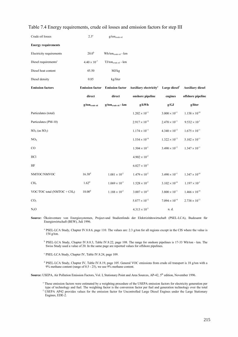
Table 7.4 Energy requirements, crude oil losses and emission factors for step III

Crude oil losses 2.3a g/toncrude oil

Energy requirements

Electricity requirements 20.0b Wh/toncrude oil - km

Diesel requirementsc 4.40 × 10-7 TJ/toncrude oil - km

Diesel heat content 45.50 MJ/kg

Diesel density 0.85 kg/liter

Emission factors Emission factor Emission factor Auxiliary electricitye Large dieself Auxiliary diesel

direct direct onshore pipeline engines offshore pipeline

g/toncrude oil g/toncrude oil - km g/kWh g/GJ g/liter

Particulates (total) 1.202 × 10+1 3.000 × 10+1 1.158 × 10+0

Particulates (PM-10) 2.917 × 10+0 2.470 × 10+1 9.532 × 10-1

SOX (as SO2) 1.174 × 10+1 4.340 × 10+2 1.675 × 10+1

NOX 1.534 × 10+0 1.322 × 10+3 5.102 × 10+1

CO 1.504 × 10-1 3.490 × 10+2 1.347 × 10+1

HCl 4.902 × 10-2

HF 6.027 × 10-3

NMTOC/NMVOC 16.38d 1.081 × 10-2 1.479 × 10-2 3.490 × 10+1 1.347 × 10+0

CH4 1.62d 1.069 × 10-3 1.528 × 10-2 3.102 × 10+0 1.197 × 10-1

VOC/TOC total (NMTOC + CH4) 18.00d 1.188 × 10-2 3.007 × 10-2 3.800 × 10+1 1.466 × 10+0

CO2 5.877 × 10+2 7.094 × 10+4 2.738 × 10+3

N2O 4.313 × 10-3 n. d.


a PSEL-LCA Study, Chapter IV.8.8.6, page 110. The values are: 2.3 g/ton for all regions except in the CIS where the value is 154 g/ton.

b PSEL-LCA Study, Chapter IV.8.8.3, Table IV.8.22, page 108. The range for onshore pipelines is 17-33 Wh/ton - km. The Swiss Study used a value of 20. In the same page are reported values for offshore pipelines.

c PSEL-LCA Study, Chapter IV, Table IV.8.24, page 109.

d PSEL-LCA Study, Chapter IV, Table IV.8.19, page 105. General VOC emissions from crude oil transport is 18 g/ton with a 9% methane content (range of 0.5 - 25), we use 9% methane content.

Source: USEPA, Air Pollution Emission Factors, Vol. I, Stationary Point and Area Sources, AP-42, 5th edition, November 1996.

e These emission factors were estimated by a weighting procedure of the USEPA emission factors for electricity generation per type of technology and fuel. The weighting factor is the conversion factor per fuel and generation technology over the total

f USEPA AP42 provides values for the emission factor for Uncontrolled Large Diesel Engines under the Large Stationary Engines, EDE-2.

215

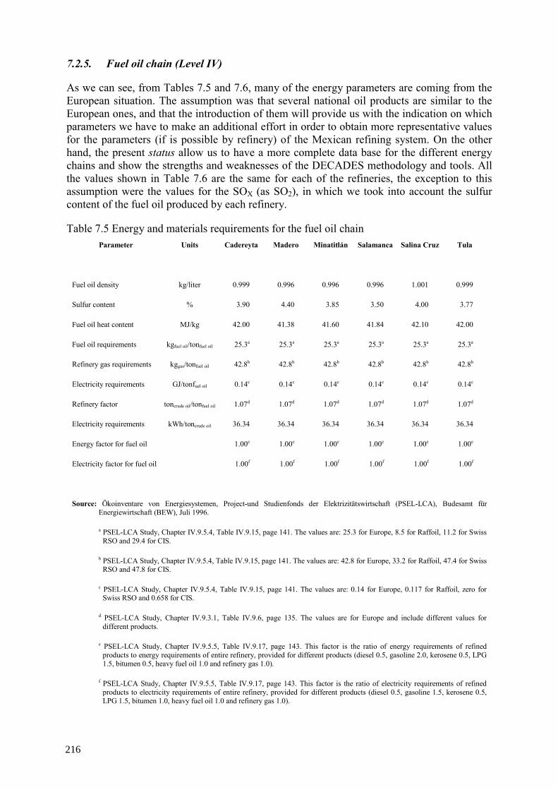
7.2.5. Fuel oil chain (Level IV)

As we can see, from Tables 7.5 and 7.6, many of the energy parameters are coming from the European situation. The assumption was that several national oil products are similar to the European ones, and that the introduction of them will provide us with the indication on which parameters we have to make an additional effort in order to obtain more representative values for the parameters (if is possible by refinery) of the Mexican refining system. On the other hand, the present status allow us to have a more complete data base for the different energy chains and show the strengths and weaknesses of the DECADES methodology and tools. All the values shown in Table 7.6 are the same for each of the refineries, the exception to this assumption were the values for the SOX (as SO2), in which we took into account the sulfur content of the fuel oil produced by each refinery.

Table 7.5 Energy and materials requirements for the fuel oil chain Parameter Units Cadereyta Madero Minatitlán Salamanca Salina Cruz Tula

Fuel oil density kg/liter 0.999 0.996 0.996 0.996 1.001 0.999

Sulfur content % 3.90 4.40 3.85 3.50 4.00 3.77

Fuel oil heat content MJ/kg 42.00 41.38 41.60 41.84 42.10 42.00

Fuel oil requirements kgfuel oil/tonfuel oil 25.3a 25.3a 25.3a 25.3a 25.3a 25.3a

Refinery gas requirements kggas/tonfuel oil 42.8b 42.8b 42.8b 42.8b 42.8b 42.8b

Electricity requirements GJ/tonfuel oil 0.14c 0.14c 0.14c 0.14c 0.14c 0.14c

Refinery factor toncrude oil/tonfuel oil 1.07d 1.07d 1.07d 1.07d 1.07d 1.07d

Electricity requirements kWh/toncrude oil 36.34 36.34 36.34 36.34 36.34 36.34

Energy factor for fuel oil 1.00e 1.00e 1.00e 1.00e 1.00e 1.00e

Electricity factor for fuel oil 1.00f 1.00f 1.00f 1.00f 1.00f 1.00f


a PSEL-LCA Study, Chapter IV.9.5.4, Table IV.9.15, page 141. The values are: 25.3 for Europe, 8.5 for Raffoil, 11.2 for Swiss RSO and 29.4 for CIS.

b PSEL-LCA Study, Chapter IV.9.5.4, Table IV.9.15, page 141. The values are: 42.8 for Europe, 33.2 for Raffoil, 47.4 for Swiss RSO and 47.8 for CIS.

c PSEL-LCA Study, Chapter IV.9.5.4, Table IV.9.15, page 141. The values are: 0.14 for Europe, 0.117 for Raffoil, zero for Swiss RSO and 0.658 for CIS.

d PSEL-LCA Study, Chapter IV.9.3.1, Table IV.9.6, page 135. The values are for Europe and include different values for different products.

e PSEL-LCA Study, Chapter IV.9.5.5, Table IV.9.17, page 143. This factor is the ratio of energy requirements of refined products to energy requirements of entire refinery, provided for different products (diesel 0.5, gasoline 2.0, kerosene 0.5, LPG 1.5, bitumen 0.5, heavy fuel oil 1.0 and refinery gas 1.0).

f PSEL-LCA Study, Chapter IV.9.5.5, Table IV.9.17, page 143. This factor is the ratio of electricity requirements of refined products to electricity requirements of entire refinery, provided for different products (diesel 0.5, gasoline 1.5, kerosene 0.5, LPG 1.5, bitumen 1.0, heavy fuel oil 1.0 and refinery gas 1.0).

216

7.2.6. Fuel oil transportation (Level V)

Pipeline, ship, train and truck perform fuel oil transportation from the processing facilities to the power utilities. The type of transportation depends on the specific power utility location, the transport infrastructure and logistics considerations.

Due to the fact that the WASP model is a one-node model, and that the Mexican electric system is a very scattered system of power utilities it was necessary to put the power utilities into several groups (see Chapter 4) according to similar installed capacities. This solves the problem represented by the one node limitation of WASP; however it gives rise to several problems in the transportation step from the refinery to the power plant. Of course, these problems would not be present with a several node WASP version, since, in that case, WASP could handle a regional electrical system, avoiding, in principle, the problem of different transportation modes.

These problems are present in the steam and turbo gas plants. In order to deal with these problems we made an additional assumption. This assumption was to keep the grouping of the power plants and consider the actual transportation mode and traveled distance, as well as, fuel's volume transported, the emission factors of the fuel used in each transportation mode and the amount of fuel consumed in the transportation mode per ton of fuel oil transported and per kilometre and estimate an equivalent distance for the group.

Clearly, this procedure will give us different distances for the different pollutants and the criteria were to choose the distance associated with the CO2, the major pollutant. Table 7.7 shows the estimated distances for all steam groups.

Table 7.8 shows the energy requirements and fuel oil losses during this transportation step. According to the consulted literature there are fuel oil losses due to spills and accidents. On the other hand there are electricity requirements, which contribute to the indirect emissions, as well as, those resulting from the use of diesel for the trains, trucks and ships. For the emission factors associated with this transportation step, Table 7.9 shows the values as well as the source of the factors. According to the consulted literature there are not noticeable VOC emissions from transporting heavy refined products, such as diesel and fuel oil, however there are values for gasoline and jet fuel. Therefore, there are not direct emissions for this transportation step and the factors shown in Table 7.9 are related to the auxiliary fuels -diesel and electricity- and correspond to indirect emissions.

7.2.7. Fuel oil electricity generation (Level VI)

The electricity generation step and the crude oil refining step are the more energy consuming steps of the whole oil chain. However, the electricity generation step is by all means the most energy-consuming step of these two activities in the chain. Therefore, is of the major importance to carry out a complete and detailed analysis of the data on energy consumption and emissions during this part of the chain.

The detailed analysis of the electricity generation step was carried out in the plant-level analysis of expansion alternatives (Chapter 5). For the expansion analysis it was necessary to consider, in detail, parameters such as the efficiency, heating value, specific consumption, net heat value, fuels and their characteristics, emission factors and control devices, costs, etc., for all the power plants -existing and additional- in the expansion alternatives. In consequence, the most convenient action is to refer to the reader to Chapter 5 for a detailed analysis on the relevant parameters for this step of the chain.

217

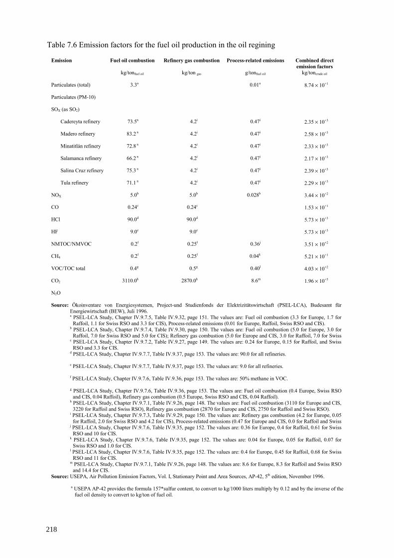
Table 7.6 Emission factors for the fuel oil production in the oil regining

Emission Fuel oil combustion Refinery gas combustion Process-related emissions Combined direct emission factors

kg/tonfuel oil kg/ton gas g/tonfuel oil kg/toncrude oil

Particulates (total) 3.3a 0.01a 8.74 × 10+1

Particulates (PM-10)

SOX (as SO2)

Cadereyta refinery 73.5n 4.2i 0.47i 2.35 × 10+3

Madero refinery 83.2 n 4.2i 0.47i 2.58 × 10+3

Minatitlán refinery 72.8 n 4.2i 0.47i 2.33 × 10+3

Salamanca refinery 66.2 n 4.2i 0.47i 2.17 × 10+3

Salina Cruz refinery 75.3 n 4.2i 0.47i 2.39 × 10+3

Tula refinery 71.1 n 4.2i 0.47i 2.29 × 10+3

NOX 5.0b 5.0b 0.028b 3.44 × 10+2

CO 0.24c 0.24c 1.53 × 10+1

HCl 90.0d 90.0d 5.73 × 10+3

HF 9.0e 9.0e 5.73 × 10+3

NMTOC/NMVOC 0.2f 0.25f 0.36j 3.51 × 10+2

CH4 0.2f 0.25f 0.04k 5.21 × 10+1

VOC/TOC total 0.4g 0.5g 0.40l 4.03 × 10+2

CO2 3110.0h 2870.0h 8.6m 1.96 × 10+5

N2O

Source: Ökoinventare von Energiesystemen, Project-und Studienfonds der Elektrizitätswirtschaft (PSEL-LCA), Budesamt für Energiewirtschaft (BEW), Juli 1996. a PSEL-LCA Study, Chapter IV.9.7.5, Table IV.9.32, page 151. The values are: Fuel oil combustion (3.3 for Europe, 1.7 for

Raffoil, 1.1 for Swiss RSO and 3.3 for CIS), Process-related emissions (0.01 for Europe, Raffoil, Swiss RSO and CIS). b PSEL-LCA Study, Chapter IV.9.7.4, Table IV.9.30, page 150. The values are: Fuel oil combustion (5.0 for Europe, 3.0 for

Raffoil, 7.0 for Swiss RSO and 5.0 for CIS); Refinery gas combustion (5.0 for Europe and CIS, 3.0 for Raffoil, 7.0 for Swiss c PSEL-LCA Study, Chapter IV.9.7.2, Table IV.9.27, page 149. The values are: 0.24 for Europe, 0.15 for Raffoil, and Swiss

RSO and 3.3 for CIS. d PSEL-LCA Study, Chapter IV.9.7.7, Table IV.9.37, page 153. The values are: 90.0 for all refineries.

e PSEL-LCA Study, Chapter IV.9.7.7, Table IV.9.37, page 153. The values are: 9.0 for all refineries.

f PSEL-LCA Study, Chapter IV.9.7.6, Table IV.9.36, page 153. The values are: 50% methane in VOC.

g PSEL-LCA Study, Chapter IV.9.7.6, Table IV.9.36, page 153. The values are: Fuel oil combustion (0.4 Europe, Swiss RSO and CIS, 0.04 Raffoil), Refinery gas combustion (0.5 Europe, Swiss RSO and CIS, 0.04 Raffoil).

h PSEL-LCA Study, Chapter IV.9.7.1, Table IV.9.26, page 148. The values are: Fuel oil combustion (3110 for Europe and CIS, 3220 for Raffoil and Swiss RSO), Refinery gas combustion (2870 for Europe and CIS, 2750 for Raffoil and Swiss RSO).

i PSEL-LCA Study, Chapter IV.9.7.3, Table IV.9.29, page 150. The values are: Refinery gas combustion (4.2 for Europe, 0.05 for Raffoil, 2.0 for Swiss RSO and 4.2 for CIS), Process-related emissions (0.47 for Europe and CIS, 0.0 for Raffoil and Swiss

j PSEL-LCA Study, Chapter IV.9.7.6, Table IV.9.35, page 152. The values are: 0.36 for Europe, 0.4 for Raffoil, 0.61 for Swiss RSO and 10 for CIS.

k PSEL-LCA Study, Chapter IV.9.7.6, Table IV.9.35, page 152. The values are: 0.04 for Europe, 0.05 for Raffoil, 0.07 for Swiss RSO and 1.0 for CIS.

l PSEL-LCA Study, Chapter IV.9.7.6, Table IV.9.35, page 152. The values are: 0.4 for Europe, 0.45 for Raffoil, 0.68 for Swiss RSO and 11 for CIS.

m PSEL-LCA Study, Chapter IV.9.7.1, Table IV.9.26, page 148. The values are: 8.6 for Europe, 8.3 for Raffoil and Swiss RSO and 14.4 for CIS.


n USEPA AP-42 provides the formula 157*sulfur content, to convert to kg/1000 liters multiply by 0.12 and by the inverse of the fuel oil density to convert to kg/ton of fuel oil.

218

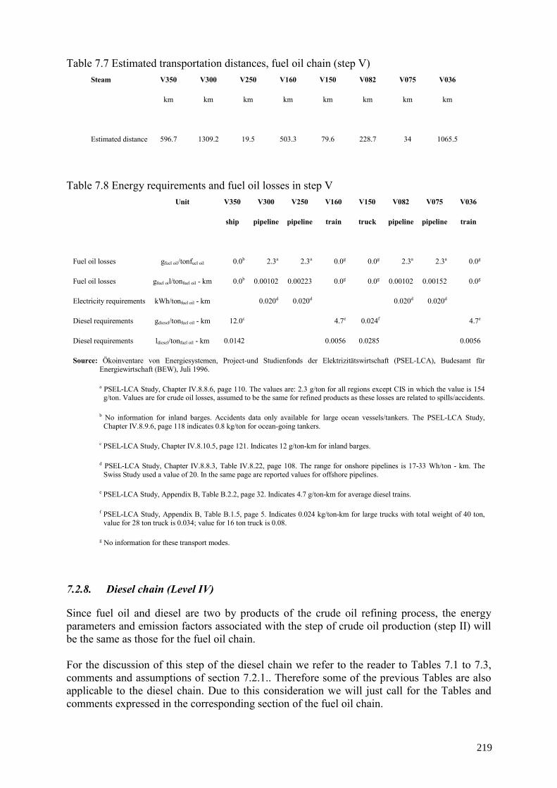
Table 7.7 Estimated transportation distances, fuel oil chain (step V) Steam V350 V300 V250 V160 V150 V082 V075 V036

km km km km km km km km

Estimated distance 596.7 1309.2 19.5 503.3 79.6 228.7 34 1065.5

Table 7.8 Energy requirements and fuel oil losses in step V Unit V350 V300 V250 V160 V150 V082 V075 V036

ship pipeline pipeline train truck pipeline pipeline train

Fuel oil losses gfuel oil/tonfuel oil 0.0b 2.3a 2.3a 0.0g 0.0g 2.3a 2.3a 0.0g

Fuel oil losses gfuel oil/tonfuel oil - km 0.0b 0.00102 0.00223 0.0g 0.0g 0.00102 0.00152 0.0g

Electricity requirements kWh/tonfuel oil - km 0.020d 0.020d 0.020d 0.020d

Diesel requirements gdiesel/tonfuel oil - km 12.0c 4.7e 0.024f 4.7e

Diesel requirements ldiesel/tonfuel oil - km 0.0142 0.0056 0.0285 0.0056


a PSEL-LCA Study, Chapter IV.8.8.6, page 110. The values are: 2.3 g/ton for all regions except CIS in which the value is 154 g/ton. Values are for crude oil losses, assumed to be the same for refined products as these losses are related to spills/accidents.

b No information for inland barges. Accidents data only available for large ocean vessels/tankers. The PSEL-LCA Study, Chapter IV.8.9.6, page 118 indicates 0.8 kg/ton for ocean-going tankers.

c PSEL-LCA Study, Chapter IV.8.10.5, page 121. Indicates 12 g/ton-km for inland barges.

d PSEL-LCA Study, Chapter IV.8.8.3, Table IV.8.22, page 108. The range for onshore pipelines is 17-33 Wh/ton - km. The Swiss Study used a value of 20. In the same page are reported values for offshore pipelines.

e PSEL-LCA Study, Appendix B, Table B.2.2, page 32. Indicates 4.7 g/ton-km for average diesel trains.

f PSEL-LCA Study, Appendix B, Table B.1.5, page 5. Indicates 0.024 kg/ton-km for large trucks with total weight of 40 ton, value for 28 ton truck is 0.034; value for 16 ton truck is 0.08.

g No information for these transport modes.

7.2.8. Diesel chain (Level IV)

Since fuel oil and diesel are two by products of the crude oil refining process, the energy parameters and emission factors associated with the step of crude oil production (step II) will be the same as those for the fuel oil chain. For the discussion of this step of the diesel chain we refer to the reader to Tables 7.1 to 7.3, comments and assumptions of section 7.2.1.. Therefore some of the previous Tables are also applicable to the diesel chain. Due to this consideration we will just call for the Tables and comments expressed in the corresponding section of the fuel oil chain.

219

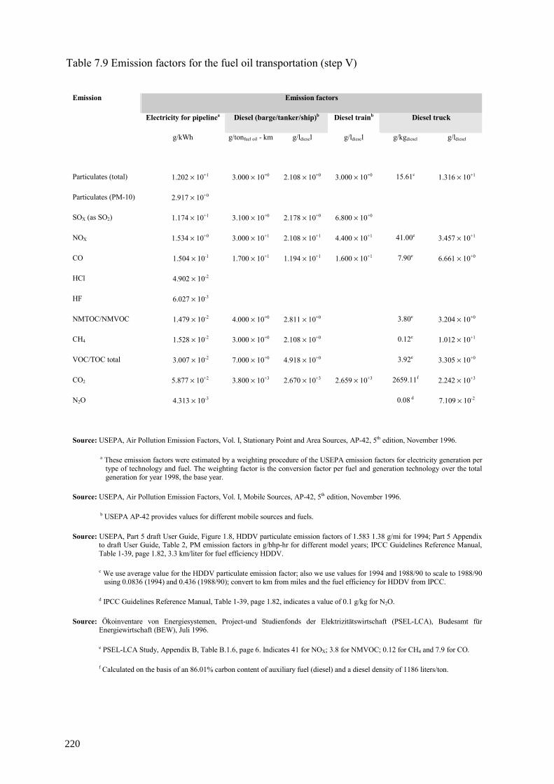
Table 7.9 Emission factors for the fuel oil transportation (step V)

Emission Emission factors

Electricity for pipelinea Diesel (barge/tanker/ship)b Diesel trainb Diesel truck

g/kWh g/tonfuel oil - km g/ldiesel g/ldiesel g/kgdiesel g/ldiesel

Particulates (total) 1.202 × 10+1 3.000 × 10+0 2.108 × 10+0 3.000 × 10+0 15.61c 1.316 × 10+1

Particulates (PM-10) 2.917 × 10+0

SOX (as SO2) 1.174 × 10+1 3.100 × 10+0 2.178 × 10+0 6.800 × 10+0

NOX 1.534 × 10+0 3.000 × 10+1 2.108 × 10+1 4.400 × 10+1 41.00e 3.457 × 10+1

CO 1.504 × 10-1 1.700 × 10+1 1.194 × 10+1 1.600 × 10+1 7.90e 6.661 × 10+0

HCl 4.902 × 10-2

HF 6.027 × 10-3

NMTOC/NMVOC 1.479 × 10-2 4.000 × 10+0 2.811 × 10+0 3.80e 3.204 × 10+0

CH4 1.528 × 10-2 3.000 × 10+0 2.108 × 10+0 0.12e 1.012 × 10+1

VOC/TOC total 3.007 × 10-2 7.000 × 10+0 4.918 × 10+0 3.92e 3.305 × 10+0

CO2 5.877 × 10+2 3.800 × 10+3 2.670 × 10+3 2.659 × 10+3 2659.11f 2.242 × 10+3

N2O 4.313 × 10-3 0.08 d 7.109 × 10-2


a These emission factors were estimated by a weighting procedure of the USEPA emission factors for electricity generation per type of technology and fuel. The weighting factor is the conversion factor per fuel and generation technology over the total generation for year 1998, the base year.

Source: USEPA, Air Pollution Emission Factors, Vol. I, Mobile Sources, AP-42, 5th edition, November 1996.

b USEPA AP-42 provides values for different mobile sources and fuels.

Source: USEPA, Part 5 draft User Guide, Figure 1.8, HDDV particulate emission factors of 1.583 1.38 g/mi for 1994; Part 5 Appendix to draft User Guide, Table 2, PM emission factors in g/bhp-hr for different model years; IPCC Guidelines Reference Manual, Table 1-39, page 1.82, 3.3 km/liter for fuel efficiency HDDV.

c We use average value for the HDDV particulate emission factor; also we use values for 1994 and 1988/90 to scale to 1988/90 using 0.0836 (1994) and 0.436 (1988/90); convert to km from miles and the fuel efficiency for HDDV from IPCC.

d IPCC Guidelines Reference Manual, Table 1-39, page 1.82, indicates a value of 0.1 g/kg for N2O.


e PSEL-LCA Study, Appendix B, Table B.1.6, page 6. Indicates 41 for NOX; 3.8 for NMVOC; 0.12 for CH4 and 7.9 for CO.

f Calculated on the basis of an 86.01% carbon content of auxiliary fuel (diesel) and a diesel density of 1186 liters/ton.

220

7.2.9. Diesel transportation (Level III) As in the fuel oil chain, the second main assumption was to take into account just the pipelines from the marine regions and their length up to the coastal terminal of Dos Bocas and from there to the distribution centre of Nuevo Teapa and finally to each one of the processing centres. The offshore pipeline length to Dos Bocas terminal was estimated in 163.2 km; form Dos Bocas terminal to Nuevo Teapa distribution centre was estimated in 144 km. To these distances we have to add the pipeline length up to each one of the processing facilities.

These facilities are located at the southeast, central and northeast parts of the country. However, for the expansion analysis it was necessary to group 27 power plants with 59 generation units and capacities between 44 and 12 MW into three general groups (TG42, TG30 and TG14). These generation units are scattered along the whole country, 35 consume diesel, 20 natural gas and diesel and 4 natural gas. Therefore, it was necessary to assign them an input fuel type and a supply processing facility. Since most of the generation units consume diesel and this fuel has a more flexible transportation infrastructure, than natural gas, it was decided to use diesel as fuel type for these plant's grouping.

Finally, the diesel supply processing facility was select as the Tula’s refinery. The reason was that this facility is located near the geographical center of the group of generation plants. The crude oil pipeline that supplies crude oil to this refining facility has an average length of 923 km. It is important to recognize that part of this pipeline length is offshore and part is onshore. This was taken into account in the data preparation.

For step III, we need data on the crude oil losses, the electricity requirements and diesel requirements for the offshore pipeline part. Again, the PSEL-LCA, 1996, provides us with the required information. Two contributions have to be considered in this step since we have direct and indirect contributions to the emission. Direct contributions are the result of the NMTOC/NMVOC, methane and VOC/TOC total (NMTOC + methane). Indirect contributions are originated in the electricity that is used and the diesel consumed by the diesel engines in the offshore facilities. These factors are shown in Table 7.10.

7.2.10. Crude oil processing in the diesel chain (Level IV) For this step of the diesel chain, some energy parameters will change in comparison with the fuel oil case. Specifically, the parameters that are different are: diesel density, heat content, energy factor for diesel, electricity factor for diesel, electricity requirements and the refinery factor. The energy and emission factors are shown in Table 7.11 and 7.13.

7.2.11. Diesel transportation (Level V) Pipeline, ship, train and truck perform diesel transportation from the processing facilities to the power utilities. The type of transportation depends on the specific power utility location, the transport infrastructure and logistics considerations.

As in the case of the fuel oil chain, in this step of the diesel chain, we also face the same type of problems originated by the expansion grouping of power plants and the different transportation modes for diesel. In order to solve these problems we made the same assumptions as in the fuel oil chain, section 7.2.1. and follow the same procedure for the estimation of the diesel transportation distances. Taking into account that the processing centre that provides diesel to this group of power plants is the Tula's refinery, the estimated average distances for diesel transportation to the power plants are shown in Table 7.14. Tables 7.12 and 7.15 showed the energy parameters and emission factors for the diesel transportation from the crude oil processing facilities to the power plants.

221

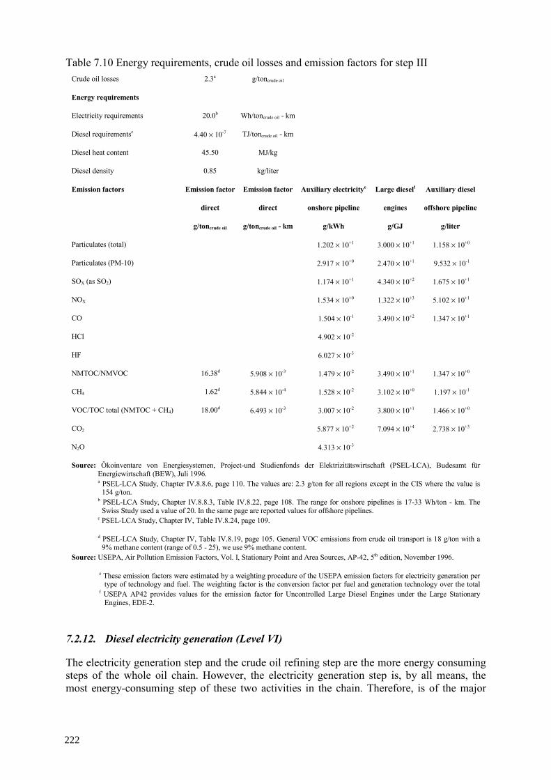
Table 7.10 Energy requirements, crude oil losses and emission factors for step III Crude oil losses 2.3a g/toncrude oil

Energy requirements

Electricity requirements 20.0b Wh/toncrude oil - km

Diesel requirementsc 4.40 × 10-7 TJ/toncrude oil - km


Diesel density 0.85 kg/liter

Emission factors Emission factor Emission factor Auxiliary electricitye Large dieself Auxiliary diesel

direct direct onshore pipeline engines offshore pipeline

g/toncrude oil g/toncrude oil - km g/kWh g/GJ g/liter

Particulates (total) 1.202 × 10+1 3.000 × 10+1 1.158 × 10+0

Particulates (PM-10) 2.917 × 10+0 2.470 × 10+1 9.532 × 10-1

SOX (as SO2) 1.174 × 10+1 4.340 × 10+2 1.675 × 10+1

NOX 1.534 × 10+0 1.322 × 10+3 5.102 × 10+1

CO 1.504 × 10-1 3.490 × 10+2 1.347 × 10+1

HCl 4.902 × 10-2

HF 6.027 × 10-3

NMTOC/NMVOC 16.38d 5.908 × 10-3 1.479 × 10-2 3.490 × 10+1 1.347 × 10+0

CH4 1.62d 5.844 × 10-4 1.528 × 10-2 3.102 × 10+0 1.197 × 10-1

VOC/TOC total (NMTOC + CH4) 18.00d 6.493 × 10-3 3.007 × 10-2 3.800 × 10+1 1.466 × 10+0

CO2 5.877 × 10+2 7.094 × 10+4 2.738 × 10+3

N2O 4.313 × 10-3

Source: Ökoinventare von Energiesystemen, Project-und Studienfonds der Elektrizitätswirtschaft (PSEL-LCA), Budesamt für Energiewirtschaft (BEW), Juli 1996. a PSEL-LCA Study, Chapter IV.8.8.6, page 110. The values are: 2.3 g/ton for all regions except in the CIS where the value is

154 g/ton. b PSEL-LCA Study, Chapter IV.8.8.3, Table IV.8.22, page 108. The range for onshore pipelines is 17-33 Wh/ton - km. The

Swiss Study used a value of 20. In the same page are reported values for offshore pipelines. c PSEL-LCA Study, Chapter IV, Table IV.8.24, page 109.

d PSEL-LCA Study, Chapter IV, Table IV.8.19, page 105. General VOC emissions from crude oil transport is 18 g/ton with a 9% methane content (range of 0.5 - 25), we use 9% methane content.


e These emission factors were estimated by a weighting procedure of the USEPA emission factors for electricity generation per type of technology and fuel. The weighting factor is the conversion factor per fuel and generation technology over the total

f USEPA AP42 provides values for the emission factor for Uncontrolled Large Diesel Engines under the Large Stationary Engines, EDE-2.

7.2.12. Diesel electricity generation (Level VI)

The electricity generation step and the crude oil refining step are the more energy consuming steps of the whole oil chain. However, the electricity generation step is, by all means, the most energy-consuming step of these two activities in the chain. Therefore, is of the major

222

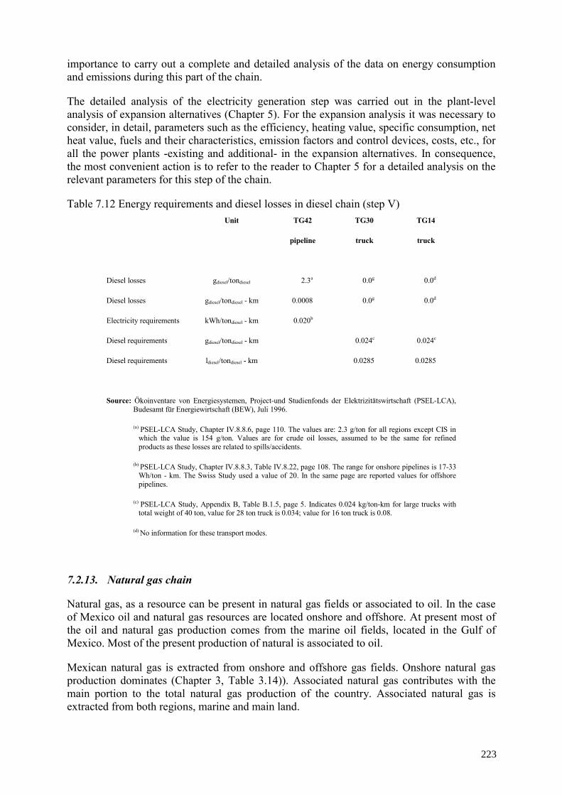
importance to carry out a complete and detailed analysis of the data on energy consumption and emissions during this part of the chain.


Table 7.12 Energy requirements and diesel losses in diesel chain (step V) Unit TG42 TG30 TG14

pipeline truck truck

Diesel losses gdiesel/tondiesel 2.3a 0.0g 0.0d

Diesel losses gdiesel/tondiesel - km 0.0008 0.0g 0.0d

Electricity requirements kWh/tondiesel - km 0.020b

Diesel requirements gdiesel/tondiesel - km 0.024c 0.024c

Diesel requirements ldiesel/tondiesel - km 0.0285 0.0285


(a) PSEL-LCA Study, Chapter IV.8.8.6, page 110. The values are: 2.3 g/ton for all regions except CIS in which the value is 154 g/ton. Values are for crude oil losses, assumed to be the same for refined products as these losses are related to spills/accidents.

(b) PSEL-LCA Study, Chapter IV.8.8.3, Table IV.8.22, page 108. The range for onshore pipelines is 17-33 Wh/ton - km. The Swiss Study used a value of 20. In the same page are reported values for offshore pipelines.

(c) PSEL-LCA Study, Appendix B, Table B.1.5, page 5. Indicates 0.024 kg/ton-km for large trucks with total weight of 40 ton, value for 28 ton truck is 0.034; value for 16 ton truck is 0.08.

(d) No information for these transport modes.

7.2.13. Natural gas chain

Natural gas, as a resource can be present in natural gas fields or associated to oil. In the case of Mexico oil and natural gas resources are located onshore and offshore. At present most of the oil and natural gas production comes from the marine oil fields, located in the Gulf of Mexico. Most of the present production of natural is associated to oil.

Mexican natural gas is extracted from onshore and offshore gas fields. Onshore natural gas production dominates (Chapter 3, Table 3.14)). Associated natural gas contributes with the main portion to the total natural gas production of the country. Associated natural gas is extracted from both regions, marine and main land.

223

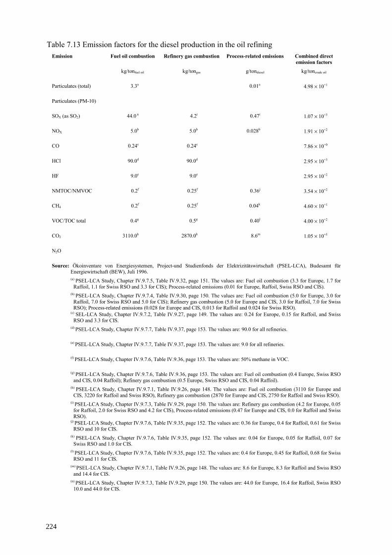
Table 7.13 Emission factors for the diesel production in the oil refining Emission Fuel oil combustion Refinery gas combustion Process-related emissions Combined direct

emission factors

kg/tonfuel oil kg/tongas g/tondiesel kg/toncrude oil

Particulates (total) 3.3a 0.01a 4.98 × 10+1


SOX (as SO2) 44.0 n 4.2i 0.47i 1.07 × 10+3

NOX 5.0b 5.0b 0.028b 1.91 × 10+2

CO 0.24c 0.24c 7.86 × 10+0

HCl 90.0d 90.0d 2.95 × 10+3

HF 9.0e 9.0e 2.95 × 10+2

NMTOC/NMVOC 0.2f 0.25f 0.36j 3.54 × 10+2

CH4 0.2f 0.25f 0.04k 4.60 × 10+1

VOC/TOC total 0.4g 0.5g 0.40l 4.00 × 10+2

CO2 3110.0h 2870.0h 8.6m 1.05 × 10+5

N2O

Source: Ökoinventare von Energiesystemen, Project-und Studienfonds der Elektrizitätswirtschaft (PSEL-LCA), Budesamt für Energiewirtschaft (BEW), Juli 1996. (a) PSEL-LCA Study, Chapter IV.9.7.5, Table IV.9.32, page 151. The values are: Fuel oil combustion (3.3 for Europe, 1.7 for

Raffoil, 1.1 for Swiss RSO and 3.3 for CIS); Process-related emissions (0.01 for Europe, Raffoil, Swiss RSO and CIS). (b) PSEL-LCA Study, Chapter IV.9.7.4, Table IV.9.30, page 150. The values are: Fuel oil combustion (5.0 for Europe, 3.0 for

Raffoil, 7.0 for Swiss RSO and 5.0 for CIS); Refinery gas combustion (5.0 for Europe and CIS, 3.0 for Raffoil, 7.0 for Swiss RSO); Process-related emissions (0.028 for Europe and CIS, 0.013 for Raffoil and 0.024 for Swiss RSO).

(c) SEL-LCA Study, Chapter IV.9.7.2, Table IV.9.27, page 149. The values are: 0.24 for Europe, 0.15 for Raffoil, and Swiss RSO and 3.3 for CIS.

(d) PSEL-LCA Study, Chapter IV.9.7.7, Table IV.9.37, page 153. The values are: 90.0 for all refineries.

(e) PSEL-LCA Study, Chapter IV.9.7.7, Table IV.9.37, page 153. The values are: 9.0 for all refineries.

(f) PSEL-LCA Study, Chapter IV.9.7.6, Table IV.9.36, page 153. The values are: 50% methane in VOC.

(g) PSEL-LCA Study, Chapter IV.9.7.6, Table IV.9.36, page 153. The values are: Fuel oil combustion (0.4 Europe, Swiss RSO and CIS, 0.04 Raffoil); Refinery gas combustion (0.5 Europe, Swiss RSO and CIS, 0.04 Raffoil).

(h) PSEL-LCA Study, Chapter IV.9.7.1, Table IV.9.26, page 148. The values are: Fuel oil combustion (3110 for Europe and CIS, 3220 for Raffoil and Swiss RSO), Refinery gas combustion (2870 for Europe and CIS, 2750 for Raffoil and Swiss RSO).

(i) PSEL-LCA Study, Chapter IV.9.7.3, Table IV.9.29, page 150. The values are: Refinery gas combustion (4.2 for Europe, 0.05 for Raffoil, 2.0 for Swiss RSO and 4.2 for CIS), Process-related emissions (0.47 for Europe and CIS, 0.0 for Raffoil and Swiss RSO).

(j) PSEL-LCA Study, Chapter IV.9.7.6, Table IV.9.35, page 152. The values are: 0.36 for Europe, 0.4 for Raffoil, 0.61 for Swiss RSO and 10 for CIS.

(k) PSEL-LCA Study, Chapter IV.9.7.6, Table IV.9.35, page 152. The values are: 0.04 for Europe, 0.05 for Raffoil, 0.07 for Swiss RSO and 1.0 for CIS.

(l) PSEL-LCA Study, Chapter IV.9.7.6, Table IV.9.35, page 152. The values are: 0.4 for Europe, 0.45 for Raffoil, 0.68 for Swiss RSO and 11 for CIS.

(m) PSEL-LCA Study, Chapter IV.9.7.1, Table IV.9.26, page 148. The values are: 8.6 for Europe, 8.3 for Raffoil and Swiss RSO and 14.4 for CIS.

(n) PSEL-LCA Study, Chapter IV.9.7.3, Table IV.9.29, page 150. The values are: 44.0 for Europe, 16.4 for Raffoil, Swiss RSO 10.0 and 44.0 for CIS.

224

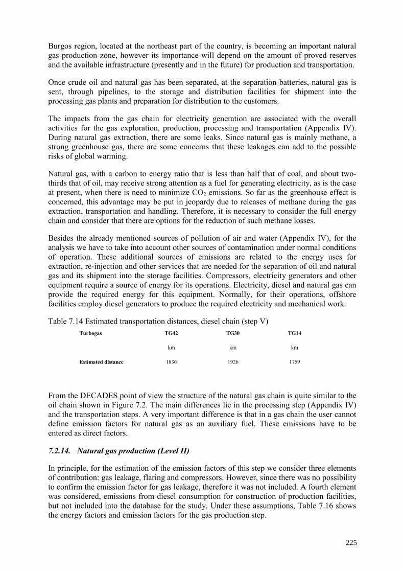
Burgos region, located at the northeast part of the country, is becoming an important natural gas production zone, however its importance will depend on the amount of proved reserves and the available infrastructure (presently and in the future) for production and transportation.

Once crude oil and natural gas has been separated, at the separation batteries, natural gas is sent, through pipelines, to the storage and distribution facilities for shipment into the processing gas plants and preparation for distribution to the customers.

The impacts from the gas chain for electricity generation are associated with the overall activities for the gas exploration, production, processing and transportation (Appendix IV). During natural gas extraction, there are some leaks. Since natural gas is mainly methane, a strong greenhouse gas, there are some concerns that these leakages can add to the possible risks of global warming.

Natural gas, with a carbon to energy ratio that is less than half that of coal, and about two-thirds that of oil, may receive strong attention as a fuel for generating electricity, as is the case at present, when there is need to minimize CO2 emissions. So far as the greenhouse effect is concerned, this advantage may be put in jeopardy due to releases of methane during the gas extraction, transportation and handling. Therefore, it is necessary to consider the full energy chain and consider that there are options for the reduction of such methane losses.

Besides the already mentioned sources of pollution of air and water (Appendix IV), for the analysis we have to take into account other sources of contamination under normal conditions of operation. These additional sources of emissions are related to the energy uses for extraction, re-injection and other services that are needed for the separation of oil and natural gas and its shipment into the storage facilities. Compressors, electricity generators and other equipment require a source of energy for its operations. Electricity, diesel and natural gas can provide the required energy for this equipment. Normally, for their operations, offshore facilities employ diesel generators to produce the required electricity and mechanical work.

Table 7.14 Estimated transportation distances, diesel chain (step V) Turbogas TG42 TG30 TG14

km km km

Estimated distance 1836 1926 1759

From the DECADES point of view the structure of the natural gas chain is quite similar to the oil chain shown in Figure 7.2. The main differences lie in the processing step (Appendix IV) and the transportation steps. A very important difference is that in a gas chain the user cannot define emission factors for natural gas as an auxiliary fuel. These emissions have to be entered as direct factors.

7.2.14. Natural gas production (Level II)

In principle, for the estimation of the emission factors of this step we consider three elements of contribution: gas leakage, flaring and compressors. However, since there was no possibility to confirm the emission factor for gas leakage, therefore it was not included. A fourth element was considered, emissions from diesel consumption for construction of production facilities, but not included into the database for the study. Under these assumptions, Table 7.16 shows the energy factors and emission factors for the gas production step.

225

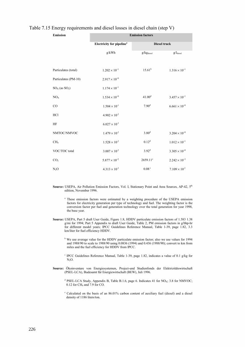
Table 7.15 Energy requirements and diesel losses in diesel chain (step V) Emission Emission factors

Electricity for pipelinea Diesel truck

g/kWh g/kgdiesel g/ldiesel

Particulates (total) 1.202 × 10+1 15.61b 1.316 × 10+1

Particulates (PM-10) 2.917 × 10+0

SOX (as SO2) 1.174 × 10+1

NOX 1.534 × 10+0 41.00d 3.457 × 10+1

CO 1.504 × 10-1 7.90d 6.661 × 10+0

HCl 4.902 × 10-2

HF 6.027 × 10-3

NMTOC/NMVOC 1.479 × 10-2 3.80d 3.204 × 10+0

CH4 1.528 × 10-2 0.12d 1.012 × 10+1

VOC/TOC total 3.007 × 10-2 3.92d 3.305 × 10+0

CO2 5.877 × 10+2 2659.11e 2.242 × 10+3

N2O 4.313 × 10-3 0.08 c 7.109 × 10-2


a These emission factors were estimated by a weighting procedure of the USEPA emission factors for electricity generation per type of technology and fuel. The weighting factor is the conversion factor per fuel and generation technology over the total generation for year 1998, the base year.

Source: USEPA, Part 5 draft User Guide, Figure 1.8, HDDV particulate emission factors of 1.583 1.38 g/mi for 1994; Part 5 Appendix to draft User Guide, Table 2, PM emission factors in g/bhp-hr for different model years; IPCC Guidelines Reference Manual, Table 1-39, page 1.82, 3.3 km/liter for fuel efficiency HDDV.

b We use average value for the HDDV particulate emission factor; also we use values for 1994 and 1988/90 to scale to 1988/90 using 0.0836 (1994) and 0.436 (1988/90); convert to km from miles and the fuel efficiency for HDDV from IPCC.

c IPCC Guidelines Reference Manual, Table 1-39, page 1.82, indicates a value of 0.1 g/kg for N2O.


d PSEL-LCA Study, Appendix B, Table B.1.6, page 6. Indicates 41 for NOX; 3.8 for NMVOC; 0.12 for CH4 and 7.9 for CO.

e Calculated on the basis of an 86.01% carbon content of auxiliary fuel (diesel) and a diesel density of 1186 liters/ton.

226

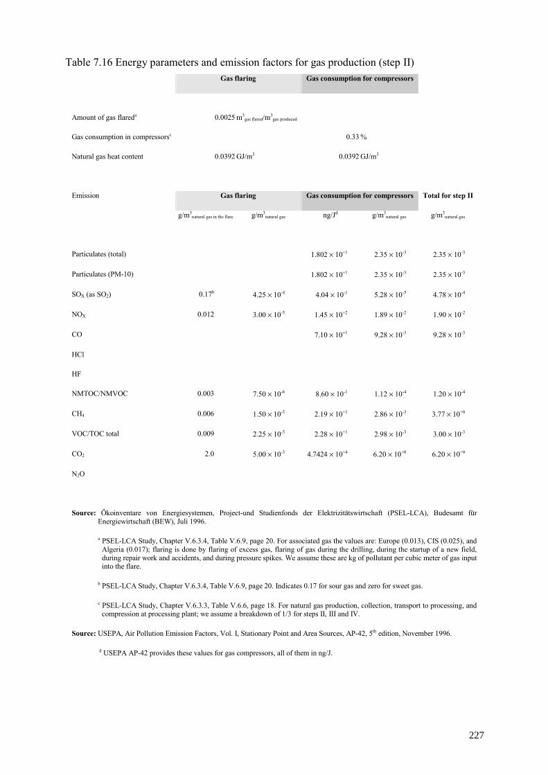
Table 7.16 Energy parameters and emission factors for gas production (step II) Gas flaring Gas consumption for compressors

Amount of gas flareda 0.0025 m3gas flared/m3

gas produced

Gas consumption in compressorsc 0.33 %

Natural gas heat content 0.0392 GJ/m3 0.0392 GJ/m3

Emission Gas flaring Gas consumption for compressors Total for step II

g/m3natural gas in the flare g/m3

natural gas ng/Jd g/m3natural gas g/m3

natural gas

Particulates (total) 1.802 × 10+1 2.35 × 10-3 2.35 × 10-3

Particulates (PM-10) 1.802 × 10+1 2.35 × 10-3 2.35 × 10-3

SOX (as SO2) 0.17b 4.25 × 10-4 4.04 × 10-1 5.28 × 10-5 4.78 × 10-4

NOX 0.012 3.00 × 10-5 1.45 × 10+2 1.89 × 10-2 1.90 × 10-2

CO 7.10 × 10+1 9.28 × 10-3 9.28 × 10-3

HCl

HF

NMTOC/NMVOC 0.003 7.50 × 10-6 8.60 × 10-1 1.12 × 10-4 1.20 × 10-4

CH4 0.006 1.50 × 10-5 2.19 × 10+1 2.86 × 10-3 3.77 × 10+0

VOC/TOC total 0.009 2.25 × 10-5 2.28 × 10+1 2.98 × 10-3 3.00 × 10-3

CO2 2.0 5.00 × 10-3 4.7424 × 10+4 6.20 × 10+0 6.20 × 10+0

N2O


a PSEL-LCA Study, Chapter V.6.3.4, Table V.6.9, page 20. For associated gas the values are: Europe (0.013), CIS (0.025), and Algeria (0.017); flaring is done by flaring of excess gas, flaring of gas during the drilling, during the startup of a new field, during repair work and accidents, and during pressure spikes. We assume these are kg of pollutant per cubic meter of gas input into the flare.

b PSEL-LCA Study, Chapter V.6.3.4, Table V.6.9, page 20. Indicates 0.17 for sour gas and zero for sweet gas.

c PSEL-LCA Study, Chapter V.6.3.3, Table V.6.6, page 18. For natural gas production, collection, transport to processing, and compression at processing plant; we assume a breakdown of 1/3 for steps II, III and IV.


d USEPA AP-42 provides these values for gas compressors, all of them in ng/J.

227

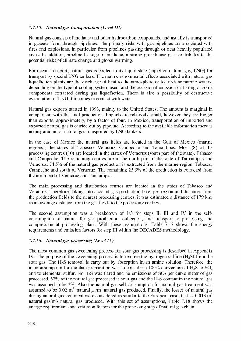
7.2.15. Natural gas transportation (Level III)

Natural gas consists of methane and other hydrocarbon compounds, and usually is transported in gaseous form through pipelines. The primary risks with gas pipelines are associated with fires and explosions, in particular from pipelines passing through or near heavily populated areas. In addition, pipeline leakage of methane, a strong greenhouse gas, contributes to the potential risks of climate change and global warming.

For ocean transport, natural gas is cooled to its liquid state (liquefied natural gas, LNG) for transport by special LNG tankers. The main environmental effects associated with natural gas liquefaction plants are the discharge of heat to the atmosphere or to fresh or marine waters, depending on the type of cooling system used, and the occasional emission or flaring of some components extracted during gas liquefaction. There is also a possibility of destructive evaporation of LNG if it comes in contact with water.

Natural gas exports started in 1993, mainly to the United States. The amount is marginal in comparison with the total production. Imports are relatively small, however they are bigger than exports, approximately, by a factor of four. In Mexico, transportation of imported and exported natural gas is carried out by pipeline. According to the available information there is no any amount of natural gas transported by LNG tankers.

In the case of Mexico the natural gas fields are located in the Gulf of Mexico (marine regions), the states of Tabasco, Veracruz, Campeche and Tamaulipas. Most (8) of the processing centres (10) are located in the states of Veracruz (south part of the state), Tabasco and Campeche. The remaining centres are in the north part of the state of Tamaulipas and Veracruz. 74.5% of the natural gas production is extracted from the marine region, Tabasco, Campeche and south of Veracruz. The remaining 25.5% of the production is extracted from the north part of Veracruz and Tamaulipas.

The main processing and distribution centres are located in the states of Tabasco and Veracruz. Therefore, taking into account gas production level per region and distances from the production fields to the nearest processing centres, it was estimated a distance of 179 km, as an average distance from the gas fields to the processing centres.

The second assumption was a breakdown of 1/3 for steps II, III and IV in the self-consumption of natural for gas production, collection, and transport to processing and compression at processing plant. With these assumptions, Table 7.17 shows the energy requirements and emission factors for step III within the DECADES methodology.

7.2.16. Natural gas processing (Level IV)

The most common gas sweetening process for sour gas processing is described in Appendix IV. The purpose of the sweetening process is to remove the hydrogen sulfide (H2S) from the sour gas. The H2S removal is carry out by absorption in an amine solution. Therefore, the main assumption for the data preparation was to consider a 100% conversion of H2S to SO2 and to elemental sulfur. No H2S was flared and no emissions of SO2 per cubic meter of gas processed. 67% of the natural gas processed is sour gas and the H2S content in the natural gas was assumed to be 2%. Also the natural gas self-consumption for natural gas treatment was assumed to be 0.02 m3 natural gas/m3 natural gas produced. Finally, the losses of natural gas during natural gas treatment were considered as similar to the European case, that is, 0.013 m3

natural gas/m3 natural gas produced. With this set of assumptions, Table 7.18 shows the energy requirements and emission factors for the processing step of natural gas chain.

228

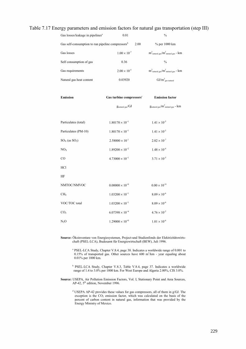
Table 7.17 Energy parameters and emission factors for natural gas transportation (step III) Gas losses/leakage in pipelinesa 0.01 %

Gas self-consumption to run pipeline compressorsb 2.00 % per 1000 km

Gas losses 1.00 × 10-7 m3natural gas/m3

natural gas - km

Self consumption of gas 0.36 %

Gas requirements 2.00 × 10-5 m3natural gas/m3

natural gas - km

Natural gas heat content 0.03920 GJ/m3gas natural

Emission Gas turbine compressorsc Emission factor

gnatural gas/GJ gnatural gas/m3natural gas - km

Particulates (total) 1.80170 × 10+1 1.41 × 10-5

Particulates (PM-10) 1.80170 × 10+1 1.41 × 10-5

SOX (as SO2) 2.58000 × 10-1 2.02 × 10-7

NOX 1.89200 × 10+2 1.48 × 10-4

CO 4.73000 × 10+1 3.71 × 10-5

HCl

HF

NMTOC/NMVOC 0.00000 × 10+0 0.00 × 10+0

CH4 1.03200 × 10+1 8.09 × 10-6

VOC/TOC total 1.03200 × 10+1 8.09 × 10-6

CO2 6.07398 × 10+4 4.76 × 10-2

N2O 1.29000 × 10+0 1.01 × 10-6

Source: Ökoinventare von Energiesystemen, Project-und Studienfonds der Elektrizitätswirts-chaft (PSEL-LCA), Budesamt für Energiewirtschaft (BEW), Juli 1996.

a PSEL-LCA Study, Chapter V.8.4, page 38. Indicates a worldwide range of 0.001 to 0.15% of transported gas. Other sources have 600 m3/km - year equaling about 0.01% per 1000 km.

b PSEL-LCA Study, Chapter V.8.3, Table V.8.4, page 37. Indicates a worldwide range of 1.4 to 3.0% per 1000 km. For West Europe and Algeria 2.00%, CIS 3.0%.


d USEPA AP-42 provides these values for gas compressors, all of them in g/GJ. The exception is the CO2 emission factor, which was calculated on the basis of the percent of carbon content in natural gas, information that was provided by the Energy Ministry of Mexico.

229

Table 7.18 Energy parameters and emission factors for gas processing (step IV) H2S content of natural gasa 2 mole %

Share of sour gas 67 %

Share of H2S flared 0 %

Natural gas self-consumption for gas treatment 0.02 m3natural gas burned/m3

natural gas produced

Natural gas losses in gas treatmentb 0.0013 m3natural gas/m3


Emission Emission factorc Emission factor

mg/m3natural gas produced g/m3


Particulates (PM-10) 3.00 × 10-4 6.00 × 10-7

SOX (as SO2) 3.40 × 10-4 6.8 × 10-2

NOX 2.0 × 10-3 4.00 × 10-5

CO 4.00 × 10-4 8.00 × 10-7


a PSEL-LCA Study, Chapter V.7.3, Table V.7.4, page 28.

b PSEL-LCA Study, Chapter V.7.6, page 30.

c PSEL-LCA Study, Chapter V.7.5, Tables V.7.6 and V.7.7, pages 29 and 30.

7.2.17. Natural gas transportation (Level V)

As in step III, the transportation mode is by pipeline, and therefore all the assumptions made for step III are applicable to the present step. However, we must remember that WASP's plant treatment of existing and additions by groups conduct us to a procedure for the estimation of the average distance for each group of plants in the expansion. This procedure was to take the actual natural gas pipeline distance to each power facility and weight them by the ratio of the consumed gas over the total gas consumption of the group of the group of plants.

The starting point for the supply was the distribution center of Ciudad Pemex in the state of Tabasco and from there each individual distance in a given group was weighted by the weighting factor of the gas consumed by the central. This was done for each of the groups of existing plants. For the additions the criteria was to consider an average distance of 300 km. Table 7.19 shows the resulting distances for this step for each of the groups. For the energy parameters and emission factors associated with this step Table 7.20 shows the values and assumptions made during the data preparation.

230

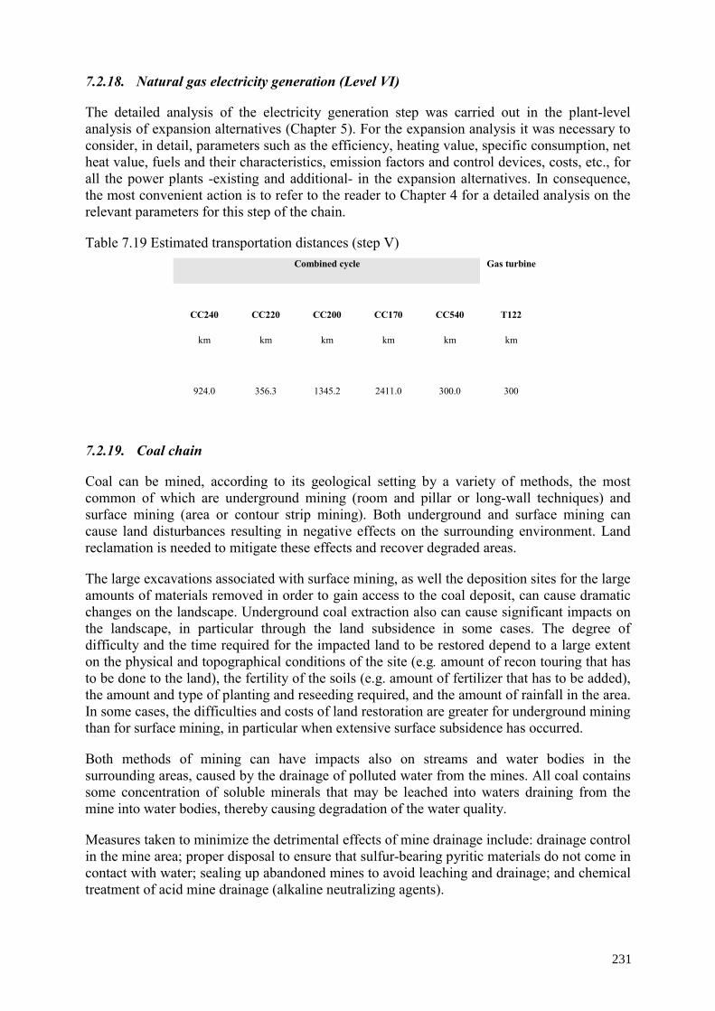
7.2.18. Natural gas electricity generation (Level VI)


Table 7.19 Estimated transportation distances (step V) Combined cycle Gas turbine

CC240 CC220 CC200 CC170 CC540 T122

km km km km km km

924.0 356.3 1345.2 2411.0 300.0 300

7.2.19. Coal chain

Coal can be mined, according to its geological setting by a variety of methods, the most common of which are underground mining (room and pillar or long-wall techniques) and surface mining (area or contour strip mining). Both underground and surface mining can cause land disturbances resulting in negative effects on the surrounding environment. Land reclamation is needed to mitigate these effects and recover degraded areas.

The large excavations associated with surface mining, as well the deposition sites for the large amounts of materials removed in order to gain access to the coal deposit, can cause dramatic changes on the landscape. Underground coal extraction also can cause significant impacts on the landscape, in particular through the land subsidence in some cases. The degree of difficulty and the time required for the impacted land to be restored depend to a large extent on the physical and topographical conditions of the site (e.g. amount of recon touring that has to be done to the land), the fertility of the soils (e.g. amount of fertilizer that has to be added), the amount and type of planting and reseeding required, and the amount of rainfall in the area. In some cases, the difficulties and costs of land restoration are greater for underground mining than for surface mining, in particular when extensive surface subsidence has occurred.

Both methods of mining can have impacts also on streams and water bodies in the surrounding areas, caused by the drainage of polluted water from the mines. All coal contains some concentration of soluble minerals that may be leached into waters draining from the mine into water bodies, thereby causing degradation of the water quality.

Measures taken to minimize the detrimental effects of mine drainage include: drainage control in the mine area; proper disposal to ensure that sulfur-bearing pyritic materials do not come in contact with water; sealing up abandoned mines to avoid leaching and drainage; and chemical treatment of acid mine drainage (alkaline neutralizing agents).

231

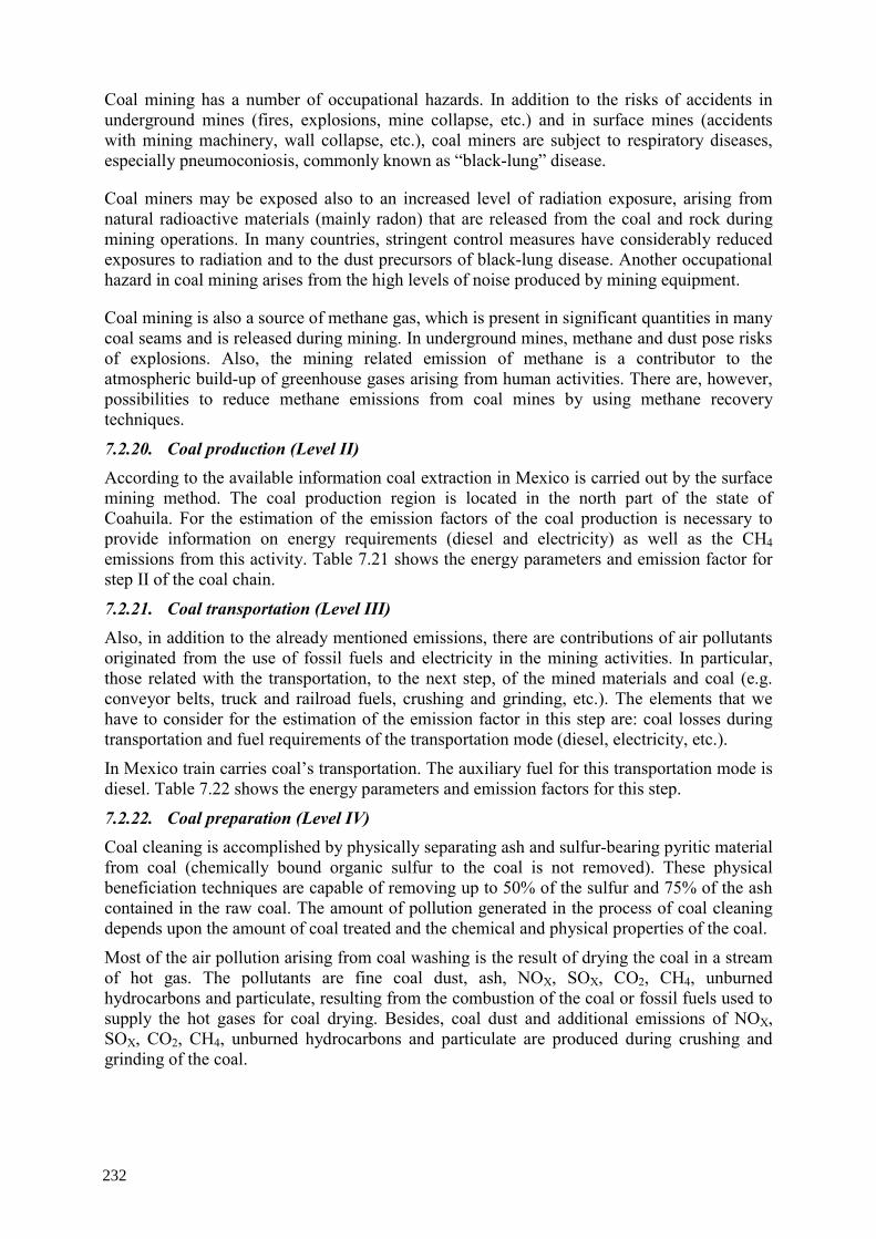
Coal mining has a number of occupational hazards. In addition to the risks of accidents in underground mines (fires, explosions, mine collapse, etc.) and in surface mines (accidents with mining machinery, wall collapse, etc.), coal miners are subject to respiratory diseases, especially pneumoconiosis, commonly known as “black-lung” disease.

Coal miners may be exposed also to an increased level of radiation exposure, arising from natural radioactive materials (mainly radon) that are released from the coal and rock during mining operations. In many countries, stringent control measures have considerably reduced exposures to radiation and to the dust precursors of black-lung disease. Another occupational hazard in coal mining arises from the high levels of noise produced by mining equipment.

Coal mining is also a source of methane gas, which is present in significant quantities in many coal seams and is released during mining. In underground mines, methane and dust pose risks of explosions. Also, the mining related emission of methane is a contributor to the atmospheric build-up of greenhouse gases arising from human activities. There are, however, possibilities to reduce methane emissions from coal mines by using methane recovery techniques.

7.2.20. Coal production (Level II) According to the available information coal extraction in Mexico is carried out by the surface mining method. The coal production region is located in the north part of the state of Coahuila. For the estimation of the emission factors of the coal production is necessary to provide information on energy requirements (diesel and electricity) as well as the CH4 emissions from this activity. Table 7.21 shows the energy parameters and emission factor for step II of the coal chain.

7.2.21. Coal transportation (Level III) Also, in addition to the already mentioned emissions, there are contributions of air pollutants originated from the use of fossil fuels and electricity in the mining activities. In particular, those related with the transportation, to the next step, of the mined materials and coal (e.g. conveyor belts, truck and railroad fuels, crushing and grinding, etc.). The elements that we have to consider for the estimation of the emission factor in this step are: coal losses during transportation and fuel requirements of the transportation mode (diesel, electricity, etc.).

In Mexico train carries coal’s transportation. The auxiliary fuel for this transportation mode is diesel. Table 7.22 shows the energy parameters and emission factors for this step.

7.2.22. Coal preparation (Level IV) Coal cleaning is accomplished by physically separating ash and sulfur-bearing pyritic material from coal (chemically bound organic sulfur to the coal is not removed). These physical beneficiation techniques are capable of removing up to 50% of the sulfur and 75% of the ash contained in the raw coal. The amount of pollution generated in the process of coal cleaning depends upon the amount of coal treated and the chemical and physical properties of the coal.

Most of the air pollution arising from coal washing is the result of drying the coal in a stream of hot gas. The pollutants are fine coal dust, ash, NOX, SOX, CO2, CH4, unburned hydrocarbons and particulate, resulting from the combustion of the coal or fossil fuels used to supply the hot gases for coal drying. Besides, coal dust and additional emissions of NOX, SOX, CO2, CH4, unburned hydrocarbons and particulate are produced during crushing and grinding of the coal.

232

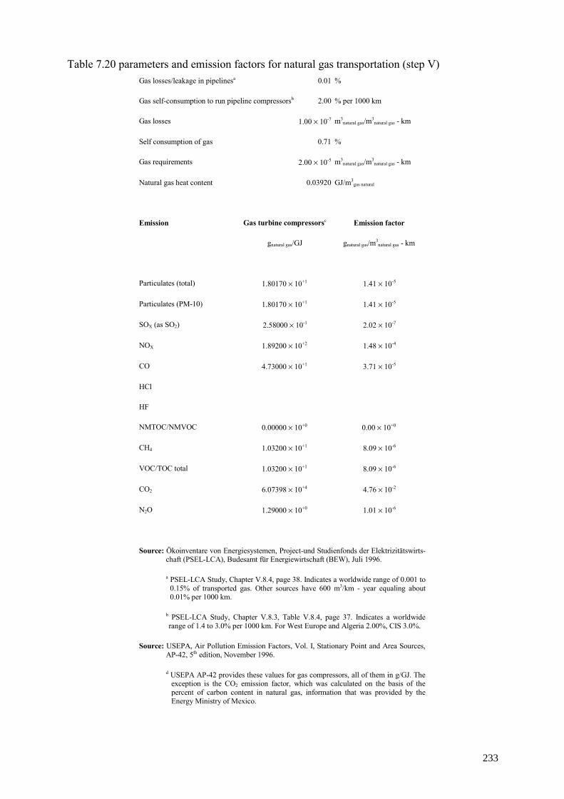
Table 7.20 parameters and emission factors for natural gas transportation (step V) Gas losses/leakage in pipelinesa 0.01 %

Gas self-consumption to run pipeline compressorsb 2.00 % per 1000 km

Gas losses 1.00 × 10-7 m3natural gas/m3

natural gas - km

Self consumption of gas 0.71 %

Gas requirements 2.00 × 10-5 m3natural gas/m3

natural gas - km

Natural gas heat content 0.03920 GJ/m3gas natural

Emission Gas turbine compressorsc Emission factor

gnatural gas/GJ gnatural gas/m3natural gas - km

Particulates (total) 1.80170 × 10+1 1.41 × 10-5

Particulates (PM-10) 1.80170 × 10+1 1.41 × 10-5

SOX (as SO2) 2.58000 × 10-1 2.02 × 10-7

NOX 1.89200 × 10+2 1.48 × 10-4

CO 4.73000 × 10+1 3.71 × 10-5

HCl

HF

NMTOC/NMVOC 0.00000 × 10+0 0.00 × 10+0

CH4 1.03200 × 10+1 8.09 × 10-6

VOC/TOC total 1.03200 × 10+1 8.09 × 10-6

CO2 6.07398 × 10+4 4.76 × 10-2

N2O 1.29000 × 10+0 1.01 × 10-6


a PSEL-LCA Study, Chapter V.8.4, page 38. Indicates a worldwide range of 0.001 to 0.15% of transported gas. Other sources have 600 m3/km - year equaling about 0.01% per 1000 km.

b PSEL-LCA Study, Chapter V.8.3, Table V.8.4, page 37. Indicates a worldwide range of 1.4 to 3.0% per 1000 km. For West Europe and Algeria 2.00%, CIS 3.0%.


d USEPA AP-42 provides these values for gas compressors, all of them in g/GJ. The exception is the CO2 emission factor, which was calculated on the basis of the percent of carbon content in natural gas, information that was provided by the Energy Ministry of Mexico.

233

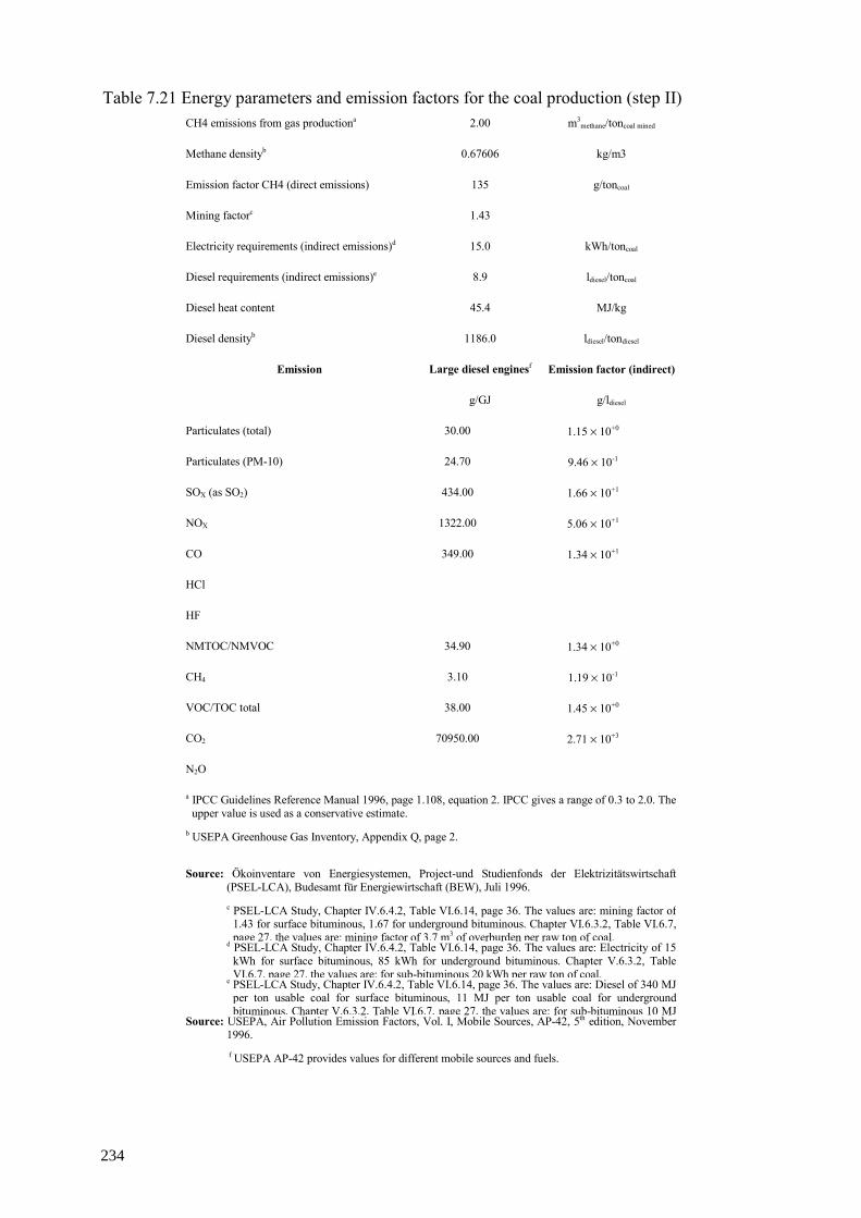
Table 7.21 Energy parameters and emission factors for the coal production (step II) CH4 emissions from gas productiona 2.00 m3

methane/toncoal mined

Methane densityb 0.67606 kg/m3

Emission factor CH4 (direct emissions) 135 g/toncoal

Mining factorc 1.43

Electricity requirements (indirect emissions)d 15.0 kWh/toncoal

Diesel requirements (indirect emissions)e 8.9 ldiesel/toncoal


Diesel densityb 1186.0 ldiesel/tondiesel

Emission Large diesel enginesf Emission factor (indirect)

g/GJ g/ldiesel

Particulates (total) 30.00 1.15 × 10+0

Particulates (PM-10) 24.70 9.46 × 10-1

SOX (as SO2) 434.00 1.66 × 10+1

NOX 1322.00 5.06 × 10+1

CO 349.00 1.34 × 10+1

HCl

HF

NMTOC/NMVOC 34.90 1.34 × 10+0

CH4 3.10 1.19 × 10-1

VOC/TOC total 38.00 1.45 × 10+0

CO2 70950.00 2.71 × 10+3

N2O

a IPCC Guidelines Reference Manual 1996, page 1.108, equation 2. IPCC gives a range of 0.3 to 2.0. The upper value is used as a conservative estimate.

b USEPA Greenhouse Gas Inventory, Appendix Q, page 2.

Source: Ökoinventare von Energiesystemen, Project-und Studienfonds der Elektrizitätswirtschaft (PSEL-LCA), Budesamt für Energiewirtschaft (BEW), Juli 1996. c PSEL-LCA Study, Chapter IV.6.4.2, Table VI.6.14, page 36. The values are: mining factor of

1.43 for surface bituminous, 1.67 for underground bituminous. Chapter VI.6.3.2, Table VI.6.7, page 27, the values are: mining factor of 3.7 m3 of overburden per raw ton of coal.

d PSEL-LCA Study, Chapter IV.6.4.2, Table VI.6.14, page 36. The values are: Electricity of 15 kWh for surface bituminous, 85 kWh for underground bituminous. Chapter V.6.3.2, Table VI.6.7, page 27, the values are: for sub-bituminous 20 kWh per raw ton of coal.

e PSEL-LCA Study, Chapter IV.6.4.2, Table VI.6.14, page 36. The values are: Diesel of 340 MJ per ton usable coal for surface bituminous, 11 MJ per ton usable coal for underground bituminous. Chapter V.6.3.2, Table VI.6.7, page 27, the values are: for sub-bituminous 10 MJ

Source: USEPA, Air Pollution Emission Factors, Vol. I, Mobile Sources, AP-42, 5th edition, November 1996. f USEPA AP-42 provides values for different mobile sources and fuels.

234

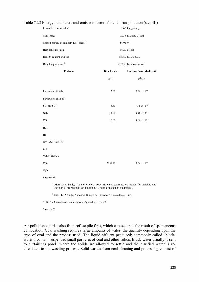
Table 7.22 Energy parameters and emission factors for coal transportation (step III) Losses in transportationa 2.00 kgcoal/toncoal

Coal losses 0.033 gcoal/toncoal - km

Carbon content of auxiliary fuel (diesel) 86.01 %

Heat content of coal 16.20 MJ/kg

Density content of dieselc 1186.0 ldiesel/tondiesel

Diesel requirementsb 0.0056 ldiesel/toncoal - km

Emission Diesel traind Emission factor (indirect)

g/GJ g/ldiesel



SOX (as SO2) 6.80 6.80 × 10+0

NOX 44.00 4.40 × 10+1

CO 16.00 1.60 × 10+1

HCl

HF

NMTOC/NMVOC

CH4

VOC/TOC total

CO2 2659.11 2.66 × 10+3

N2O

Source: [6].

a PSEL-LCA Study, Chapter VI.6.6.3, page 28. UBA estimates 0.2 kg/ton for handling and transport of brown coal (sub-bituminous). No information on bituminous.

b PSEL-LCA Study, Appendix B, page 32. Indicates 4.7 gdiesel/toncoal - km.

c USEPA, Greenhouse Gas Inventory, Appendix Q, page 2.

Source: [7].

Air pollution can rise also from refuse pile fires, which can occur as the result of spontaneous combustion. Coal washing requires large amounts of water, the quantity depending upon the type of coal and the process used. The liquid effluent produced; commonly called “black-water”, contain suspended small particles of coal and other solids. Black-water usually is sent to a “tailings pond” where the solids are allowed to settle and the clarified water is re-circulated to the washing process. Solid wastes from coal cleaning and processing consist of

235

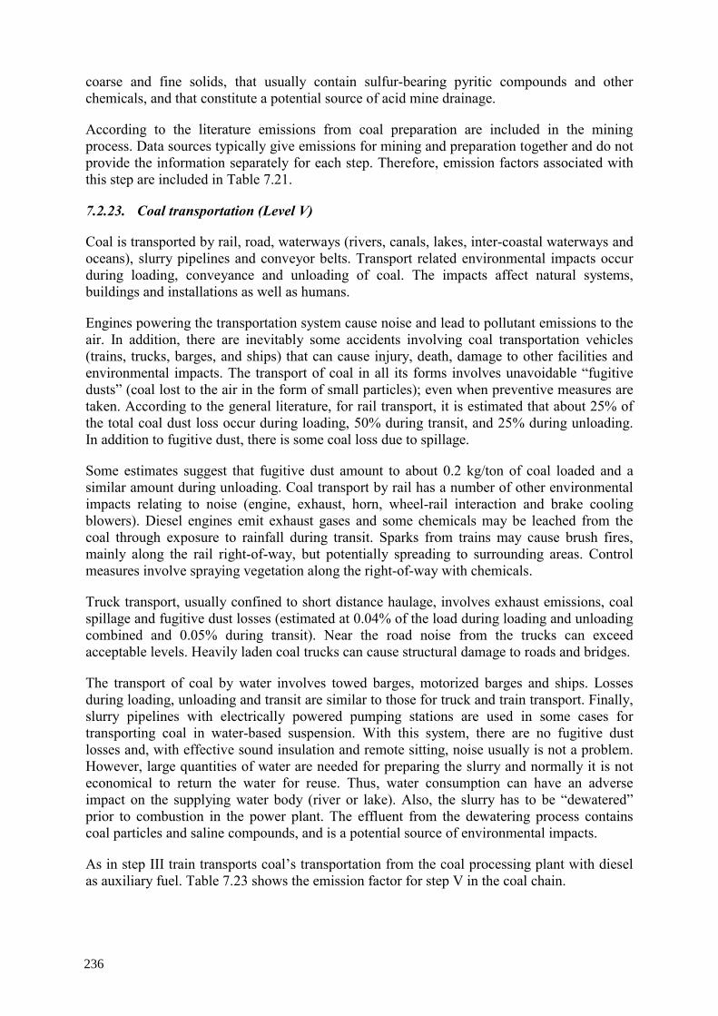
coarse and fine solids, that usually contain sulfur-bearing pyritic compounds and other chemicals, and that constitute a potential source of acid mine drainage.

According to the literature emissions from coal preparation are included in the mining process. Data sources typically give emissions for mining and preparation together and do not provide the information separately for each step. Therefore, emission factors associated with this step are included in Table 7.21.

7.2.23. Coal transportation (Level V)

Coal is transported by rail, road, waterways (rivers, canals, lakes, inter-coastal waterways and oceans), slurry pipelines and conveyor belts. Transport related environmental impacts occur during loading, conveyance and unloading of coal. The impacts affect natural systems, buildings and installations as well as humans.

Engines powering the transportation system cause noise and lead to pollutant emissions to the air. In addition, there are inevitably some accidents involving coal transportation vehicles (trains, trucks, barges, and ships) that can cause injury, death, damage to other facilities and environmental impacts. The transport of coal in all its forms involves unavoidable “fugitive dusts” (coal lost to the air in the form of small particles); even when preventive measures are taken. According to the general literature, for rail transport, it is estimated that about 25% of the total coal dust loss occur during loading, 50% during transit, and 25% during unloading. In addition to fugitive dust, there is some coal loss due to spillage.

Some estimates suggest that fugitive dust amount to about 0.2 kg/ton of coal loaded and a similar amount during unloading. Coal transport by rail has a number of other environmental impacts relating to noise (engine, exhaust, horn, wheel-rail interaction and brake cooling blowers). Diesel engines emit exhaust gases and some chemicals may be leached from the coal through exposure to rainfall during transit. Sparks from trains may cause brush fires, mainly along the rail right-of-way, but potentially spreading to surrounding areas. Control measures involve spraying vegetation along the right-of-way with chemicals.

Truck transport, usually confined to short distance haulage, involves exhaust emissions, coal spillage and fugitive dust losses (estimated at 0.04% of the load during loading and unloading combined and 0.05% during transit). Near the road noise from the trucks can exceed acceptable levels. Heavily laden coal trucks can cause structural damage to roads and bridges.

The transport of coal by water involves towed barges, motorized barges and ships. Losses during loading, unloading and transit are similar to those for truck and train transport. Finally, slurry pipelines with electrically powered pumping stations are used in some cases for transporting coal in water-based suspension. With this system, there are no fugitive dust losses and, with effective sound insulation and remote sitting, noise usually is not a problem. However, large quantities of water are needed for preparing the slurry and normally it is not economical to return the water for reuse. Thus, water consumption can have an adverse impact on the supplying water body (river or lake). Also, the slurry has to be “dewatered” prior to combustion in the power plant. The effluent from the dewatering process contains coal particles and saline compounds, and is a potential source of environmental impacts.

As in step III train transports coal’s transportation from the coal processing plant with diesel as auxiliary fuel. Table 7.23 shows the emission factor for step V in the coal chain.

236

Table 7.23 Energy parameters and emission factors for coal transportation (step III) Losses in transportationa 2.00 kgcoal/toncoal

Coal losses 0.167 gcoal/toncoal - km

Carbon content of auxiliary fuel (diesel) 86.01 %

Heat content of coal 16.20 MJ/kg

Density content of dieselc 1186.0 ldiesel/tondiesel

Diesel requirementsb 0.0056 ldiesel/toncoal - km

Emission Diesel traind Emission factor (indirect)

g/GJ g/ldiesel



SOX (as SO2) 6.80 6.80 × 10+0

NOX 44.00 4.40 × 10+1

CO 16.00 1.60 × 10+1

HCl

HF

NMTOC/NMVOC

CH4

VOC/TOC total

CO2 2659.11 2.66 × 10+3

N2O

Source: [6]

a PSEL-LCA Study, Chapter VI.6.6.3, page 28. UBA estimates 0.2 kg/ton for handling and transport of brown coal (sub-bituminous). No information on bituminous.

b PSEL-LCA Study, Appendix B, page 32. Indicates 4.7 gdiesel/toncoal - km.

c USEPA, Greenhouse Gas Inventory, Appendix Q, page 2.

Source: [7].

237

7.2.24. Coal electricity generation (Level VI)

The qualities of coal in terms of heat output per tone or amounts of ash and other wastes vary considerably. For example, lignite has a lower heat value and contains significantly more ash than hard coal.

The type and efficiency of the installed flue gas treatment system will influence the amount of solid wastes also. For example, the use of limestone injected into the combustion chamber as a means for removing sulfur increases the emissions of CO2 and the quantities of solid wastes in comparison with a plant equipped with a wet flue gas scrubbing system for sulfur control.

In addition, toxic components of the ash (metals, radio nuclides, etc.) are incorporated in the total solid waste volume from the plant using limestone injection, whereas in a plant equipped with wet scrubbers, the solid wastes from the post-combustion flue gas desulphurization process are, in essence, free of these components. This may affect the choice of systems for the management and disposal of the solid wastes. The storage of coal can present problems of spontaneous combustion, especially in the case of lower rank coals with high content of volatile compounds.

As in the case of the previous chains the emission factors for the electricity generation were discussed in detail in Chapter 3, therefore we refer to the reader to the expansion analysis chapter.

7.2.25. Nuclear chain

The nuclear energy chain is more complex than other energy chains. It has many levels and sub-levels. It can be divided into three main stages:

• The so-called front-end which extends from the mining of uranium ore until the delivery of fabricated fuel elements to the reactor site;

• Fuel use in the reactor, where fission energy is employed to produce electricity, and temporary storage at the reactor site; and,

• The so-called back-end, which starts with the shipping of spent fuel to away-from reactor storage or to a reprocessing plant ends with the final disposal of wastes from reprocessing or the encapsulates spent fuel itself.

The nuclear energy chain has been called for historical reasons “the nuclear fuel cycle”. Actually there are two options: the “open cycle” or “direct disposal” option, and the “closed cycle” or “reprocessing and recycling” option.

Some countries like USA and Sweden use the “open cycle” option, while most of the European countries (France, Germany, Belgium, Switzerland, Holland and Japan) use the “closed cycle”. Other countries like Spain, Korea, Taiwan and Mexico are still undecided with respect to this option that impacts mainly the backend of the nuclear chain.

Figure 5.3 shows the full nuclear energy chain defined in DECADES. The “Reprocessing” level and its preceding transport level should be omitted in the chain for the “open cycle”. The nuclear chain is very complex and requires a great number of steps with different technologies, with transportation steps indicated by the arrows; however its environmental impact is smaller than that generated in fossil fuel energy chains.

238

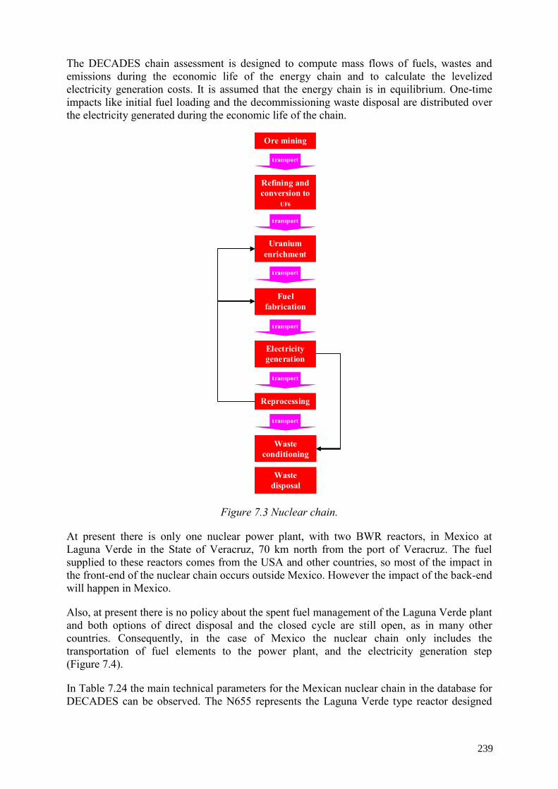
The DECADES chain assessment is designed to compute mass flows of fuels, wastes and emissions during the economic life of the energy chain and to calculate the levelized electricity generation costs. It is assumed that the energy chain is in equilibrium. One-time impacts like initial fuel loading and the decommissioning waste disposal are distributed over the electricity generated during the economic life of the chain.

Ore mining

Refining and conversion to

UF6

Uranium enrichment

Fuel fabrication


Reprocessing

Waste conditioning

Waste disposal

transport

transport

transport

transport

transport

transport

Ore mining

Refining and conversion to

UF6

Uranium enrichment

Fuel fabrication


Reprocessing

Waste conditioning

Waste disposal

transport

transport

transport

transport

transport

transport

Figure 7.3 Nuclear chain.

At present there is only one nuclear power plant, with two BWR reactors, in Mexico at Laguna Verde in the State of Veracruz, 70 km north from the port of Veracruz. The fuel supplied to these reactors comes from the USA and other countries, so most of the impact in the front-end of the nuclear chain occurs outside Mexico. However the impact of the back-end will happen in Mexico.

Also, at present there is no policy about the spent fuel management of the Laguna Verde plant and both options of direct disposal and the closed cycle are still open, as in many other countries. Consequently, in the case of Mexico the nuclear chain only includes the transportation of fuel elements to the power plant, and the electricity generation step (Figure 7.4).

In Table 7.24 the main technical parameters for the Mexican nuclear chain in the database for DECADES can be observed. The N655 represents the Laguna Verde type reactor designed

239

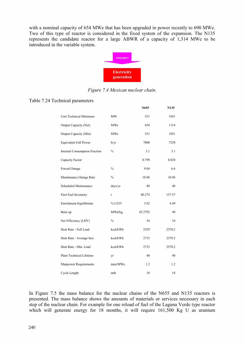
with a nominal capacity of 654 MWe that has been upgraded in power recently to 690 MWe. Two of this type of reactor is considered in the fixed system of the expansion. The N135 represents the candidate reactor for a large ABWR of a capacity of 1,314 MWe to be introduced in the variable system.


transport


transporttransport

Figure 7.4 Mexican nuclear chain.

Table 7.24 Technical parameters N655 N135

Unit Technical Minimum MW 551 1051

Output Capacity (Net) MWe 656 1314

Output Capacity (Min) MWe 551 1051

Equivalent Full Power h/yr 7000 7258

Internal Consumption Fraction % 3.1 3.1

Capacity Factor 0.799 0.828

Forced Outage % 9.04 6.6

Maintenance Outage Rate % 10.96 10.96

Scheduled Maintenance days/yr 40 40

First Fuel Inventory t 80.274 157.57

Enrichment-Equilibrium % U235 3.92 4.49

Burn up MWd/kg 45.2792 49

Net Efficiency (LHV) % 34 34

Heat Rate - Full Load kcal/kWh 2529 2570.2

Heat Rate - Average Incr. kcal/kWh 2733 2570.2

Heat Rate - Min. Load kcal/kWh 2733 2570.2

Plant Technical Lifetime yr 40 40

Manpower Requirements men/MWe 1.2 1.2

Cycle Length mth 18 18

In Figure 7.5 the mass balance for the nuclear chains of the N655 and N135 reactors is presented. The mass balance shows the amounts of materials or services necessary in each step of the nuclear chain. For example for one reload of fuel of the Laguna Verde type reactor which will generate energy for 18 months, it will require 161,500 Kg U as uranium

240

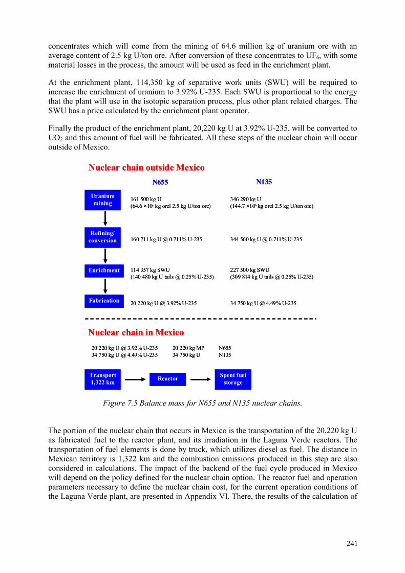
concentrates which will come from the mining of 64.6 million kg of uranium ore with an average content of 2.5 kg U/ton ore. After conversion of these concentrates to UF6, with some material losses in the process, the amount will be used as feed in the enrichment plant.

At the enrichment plant, 114,350 kg of separative work units (SWU) will be required to increase the enrichment of uranium to 3.92% U-235. Each SWU is proportional to the energy that the plant will use in the isotopic separation process, plus other plant related charges. The SWU has a price calculated by the enrichment plant operator.

Finally the product of the enrichment plant, 20,220 kg U at 3.92% U-235, will be converted to UO2 and this amount of fuel will be fabricated. All these steps of the nuclear chain will occur outside of Mexico.

Uranium mining

161 500 kg U(64.6 ×106 kg orel 2.5 kg U/ton ore)


Refining/ conversion 160 711 kg U @ 0.711% U-235 344 560 kg U @ 0.711% U-235

Enrichment 114 357 kg SWU(140 480 kg U tails @ 0.25% U-235)

227 500 kg SWU(309 814 kg U tails @ 0.25% U-235)

Fabrication 20 220 kg U @ 3.92% U-235 34 750 kg U @ 4.49% U-235

Nuclear chain in Mexico20 220 kg U @ 3.92% U-23534 750 kg U @ 4.49% U-235

20 220 kg MP34 750 kg U

N655N135

Transport 1,322 km Reactor Spent fuel

storage

Nuclear chain outside MexicoN655 N135

Uranium mining



Refining/ conversion 160 711 kg U @ 0.711% U-235 344 560 kg U @ 0.711% U-235

Enrichment 114 357 kg SWU(140 480 kg U tails @ 0.25% U-235)

227 500 kg SWU(309 814 kg U tails @ 0.25% U-235)

Fabrication 20 220 kg U @ 3.92% U-235 34 750 kg U @ 4.49% U-235

Nuclear chain in Mexico20 220 kg U @ 3.92% U-23534 750 kg U @ 4.49% U-235

20 220 kg MP34 750 kg U

N655N135

Transport 1,322 km Reactor Spent fuel

storage

Nuclear chain outside MexicoN655 N135

Figure 7.5 Balance mass for N655 and N135 nuclear chains.

The portion of the nuclear chain that occurs in Mexico is the transportation of the 20,220 kg U as fabricated fuel to the reactor plant, and its irradiation in the Laguna Verde reactors. The transportation of fuel elements is done by truck, which utilizes diesel as fuel. The distance in Mexican territory is 1,322 km and the combustion emissions produced in this step are also considered in calculations. The impact of the backend of the fuel cycle produced in Mexico will depend on the policy defined for the nuclear chain option. The reactor fuel and operation parameters necessary to define the nuclear chain cost, for the current operation conditions of the Laguna Verde plant, are presented in Appendix VI. There, the results of the calculation of

241

the nuclear fuel chain cost using the methodology described by the IAEA in the benchmarking of extended burn up study26 are presented.

7.2.26. Nuclear chain emissions

The nuclear fuel chain will produce solid, liquid and gaseous emissions. However this emissions are generally treated and contained, only emissions that are consistent with the natural background are discharged to the environment, and this is in accordance with the ALARA (“as low as reasonable acceptable”) philosophy and in some cases the “zero discharge” philosophy is applicable.

This means that most of the environmental externalities produced in the nuclear chain are in fact internalized, in contrast with the externalities produced in other energy chains, like gas, oil or coal. As a matter of fact the nuclear chain is the lowest greenhouse gas producer and the nuclear reactor will produce zero greenhouse gases during its operation. All the nuclear wastes produced in the chain, either low/medium radioactive wastes (LMLW) or high-level waste (HLW) are conditioned and stored in safe conditions.

The different steps of the nuclear chain will produce some characteristic impacts such as the mining tails in the mining step or solid CaF2 and fluorine gas in the conversion step. The enrichment step requires large quantities of water, electricity and also produces some enrichment tails. If the electricity necessary to operate these plants is produced by fossil fuels such as in the USA plants, we will have some secondary impacts in the form of air pollution coming from these plants.

All the rest of the nuclear chain steps such as fabrication or reprocessing plants, are relatively low impact with respect to the environment. Even the spent fuel storage facilities and radioactive waste repositories are safe in their design and produce a minimum impact to the environment.

The record of the transportation steps all over the nuclear chain is excellent and much better than the record of the transportation steps of the fossil chain. This is why we insist in saying that the nuclear chain has very small or almost zero externalities during normal operation, in comparison with other energy chains. If a fair comparison of technologies is to be made in the future, these large externalities of other energy chains must be evaluated and internalized in the chain.

We are not going to discuss all the impacts of the nuclear chain, because some of the impacts occur outside the boundaries of the study, in other countries. But we will discuss only the impacts of the nuclear chain in Mexico as seen in Figure 5.5. So these impacts will come mainly from the generation step of the plant, assuming that no other nuclear chain facilities will be built in the country during the term of the study. This is may not be completely true, because some spent fuel storage facilities or radioactive waste repositories may be built during the term of the study, but their specific time of construction has not been defined.

In Table 7.25, the emissions used for the nuclear chain in the study of environmental impact are shown. These emissions are typical values for BWR reactors.

26 “Water Reactor Fuel Extended Burn up Study”, IAEA Technical Report Series No. 343, Vienna, 1992.

242

7.2.27. Renewable energy chains

Renewable energy sources are of two types: the first consists of more or less continuous natural energy flow, such as sunlight, wind, waves, etc. And the second consists of natural stocks of energy, which are renewed sufficiently rapidly for human use, such as biomass, hydropower reservoirs, etc.

These energy sources are quite heterogeneous and it is difficult to split them into cycle steps like in the case of the fossil fuels to identify the environmental residuals and impacts associated with each step of the specific chain. There is also considerably less literature on this subject compared with conventional energy sources.

Notwithstanding their generally favorable impression, renewable energy sources are not without potential environmental impacts. Because they are usually much more dilute forms of energy compared with fossil fuel or nuclear energy, renewable energy sources often require large structures for a comparable amount of energy produced, which means high material requirements and land use. It is also worth remembering that large-scale developments can also have climatologically or ecological impacts resulting directly from the diversion of a natural energy flow or the intensive use of a natural energy stock. On the positive side must be considered the avoidance of adverse environmental effects associated with the types of electricity generation displaced.

Hydropower is the main contributor of the renewable energy sources to electricity generation. Substantial research and development efforts are being made aiming towards enhancing the technical and economic performance of solar, wind, biomass and other renewable energy technologies. Already, some of these technologies are economically viable in favorable locations (e. g., wind power in locations with steady strong winds, solar power in remote locations not connected to electricity distribution networks). However, it is not expected that renewable energies will provide an important amount of the world's electricity in the next few decades. Renewable energy sources for electricity generation have to meet some criteria in order to be considered, in an appropriated magnitude, as a reliable energy source. Such criteria are: the energy source should have an adequate resource base and that can be produced in quantities suitable for power generation purposes. For renewable energy sources such as solar, wind and geothermal, this implies that the natural energy can be collected in adequate quantities and converted to electricity with a practical efficiency. Also, electricity generation utilizing the energy source must be economically competitive with alternative options and, safety risks and social and environmental impacts must be acceptable and should not be higher than with competing fuels.

With regard to electricity generation system expansion, special consideration has to be given to the stochastic availability of renewable energies; that is, the intensity of wind and sunshine varies with the time of the day and the season of the year, and these variations cannot be forecasted with certainty. Therefore, the introduction of a large share of generation based on renewable energies can lead to a higher uncertainty on the reliability of supply being available when it is needed.

The following sections will examine the environmental residuals and impacts more specifically associated with the most common forms, in the Mexican generation system, of renewable energy; geothermal, hydroelectric and wind energies. It should be noted that of these, solar and wind can be used in small-scale applications as well as to generate electricity at a centralized facility. Their environmental implications for smaller uses are not only different in scale, but may differ in nature as well.

243

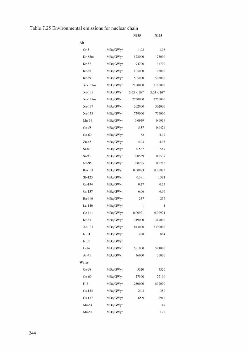
Table 7.25 Environmental emissions for nuclear chain N655 N135

Air

Cr-51 MBq/GWyr 1.08 1.08

Kr-85m MBq/GWyr 123000 123000

Kr-87 MBq/GWyr 94700 94700

Kr-88 MBq/GWyr 105000 105000

Kr-89 MBq/GWyr 505000 505000

Xe-131m MBq/GWyr 2180000 2180000

Xe-135 MBq/GWyr 3.03 × 10+8 3.03 × 10+8

Xe-135m MBq/GWyr 2750000 2750000

Xe-137 MBq/GWyr 302000 302000

Xe-138 MBq/GWyr 759000 759000

Mn-54 MBq/GWyr 0.0959 0.0959

Co-58 MBq/GWyr 5.37 0.0424

Co-60 MBq/GWyr 82 4.47

Zn-65 MBq/GWyr 4.03 4.03

Sr-89 MBq/GWyr 0.587 0.587

Sr-90 MBq/GWyr 0.0539 0.0539

Nb-95 MBq/GWyr 0.0285 0.0285

Ru-103 MBq/GWyr 0.00883 0.00883

Sb-125 MBq/GWyr 0.391 0.391

Cs-134 MBq/GWyr 0.27 0.27

Cs-137 MBq/GWyr 6.06 6.06

Ba-140 MBq/GWyr 237 237

La-140 MBq/GWyr 1 1

Ce-141 MBq/GWyr 0.00921 0.00921

Kr-85 MBq/GWyr 319000 319000

Xe-133 MBq/GWyr 843000 3390000

I-131 MBq/GWyr 30.8 884

I-133 MBq/GWyr

C-14 MBq/GWyr 591000 591000

Ar-41 MBq/GWyr 36000 36000

Water

Co-58 MBq/GWyr 5320 5320

Co-60 MBq/GWyr 27100 27100

H-3 MBq/GWyr 1250000 839000

Cs-134 MBq/GWyr 24.3 380

Cs-137 MBq/GWyr 65.9 2910

Mn-54 MBq/GWyr 149

Mn-58 MBq/GWyr 1.28

244

7.2.28. Hydroelectric chain Hydroelectric power plants contribute to the emissions due to the dam construction activities and those from decomposition of submerged biomass in hydroelectric reservoirs. When creating hydroelectric reservoirs, land surfaces containing phytomass (i. e. trees, grass, general vegetation, etc.) are flooded. The submerged phytomass undergoes anaerobic decomposition into greenhouse gasses such as CO2 and CH4, with the rate of decomposition depending on the types of phytomass and the physical and chemical properties of the water. The main conditions influencing decay rate and types of emissions are water temperature, water quality, acidity, dissolved oxygen, oxidation potential, light intensity, pressure and reservoir morphometry.

The hydro chain contains only two steps: water reservoir and hydro power plant. The specification of the chain requires installed capacity, energy storage, equivalent full power hours of operation per year, net overnight cost (NOC), NOC domestic fraction, fixed operation and maintenance costs, economic lifetime, construction period, interest during construction, CH4 emission factors from the reservoir, material requirements, etc. The emission factors for a given pollutant in the hydro chain are originated en two sources: the reservoir and the materials used. The carbon cycle in the water reservoir from which CO2 and CH4 are released, is part of a complex ecological system with interconnected chemical, physical and biotic factors (Figure 7.6).

This system being a complex one increases its complexity due to the variety of water reservoirs. In terms of the conditions for Greenhouse Gasses release one should distinguish between cold climate, humid tropical and alpine areas.

Many factors can influence emissions of Greenhouse Gasses from hydropower reservoirs (Figure 7.6), among such factors are emissions of CO2 and CH4 from biodegradation of flooded biomass on the floor of the water reservoir; natural aquatic biomass build-up and biodegradation; removal of the original vegetation which was a CO2 sink; and in view of the importance of CH4 emissions from hydropower reservoirs, special attention will be given to its global warming potential.

According to the traditional DECADES methodology, there are two types of hydropower plants: reservoir power plants and run-of-river power plants. The run-of-river power plants constitute a separate category with probably low upstream Greenhouse Gasses emissions, because of the small actual reservoir size. The run-of-river is connected to an upstream reservoir that has little useful storage volume and turbine the water as it becomes available. The water not utilized is spilled over.

On the other hand, storage power plants are connected to an upstream reservoir that has significant useful storage volume. The can store the water for periods with low power requirements and utilize it when the power demand is high. This regulation capability may be daily, weekly, seasonal or inter-annual, depending on the size of the reservoir and the pattern of water inflows.

In some sense is easy to make an inventory of the different kinds of environmental impact; on the other hand it is difficult to use quantitative measures. The environmental impact of hydropower is in many respects more direct than that of fossil fuel-fired power plant and is easy to connect a certain environmental effect to a particular hydropower site, but is considerably more difficult when it comes to the effects. The environmental effects that are typical in the case of hydropower, for instance the impact on the landscape and biodiversity, cannot be quantified in the same manner as, for example, acidification caused by sulfur emissions.

245

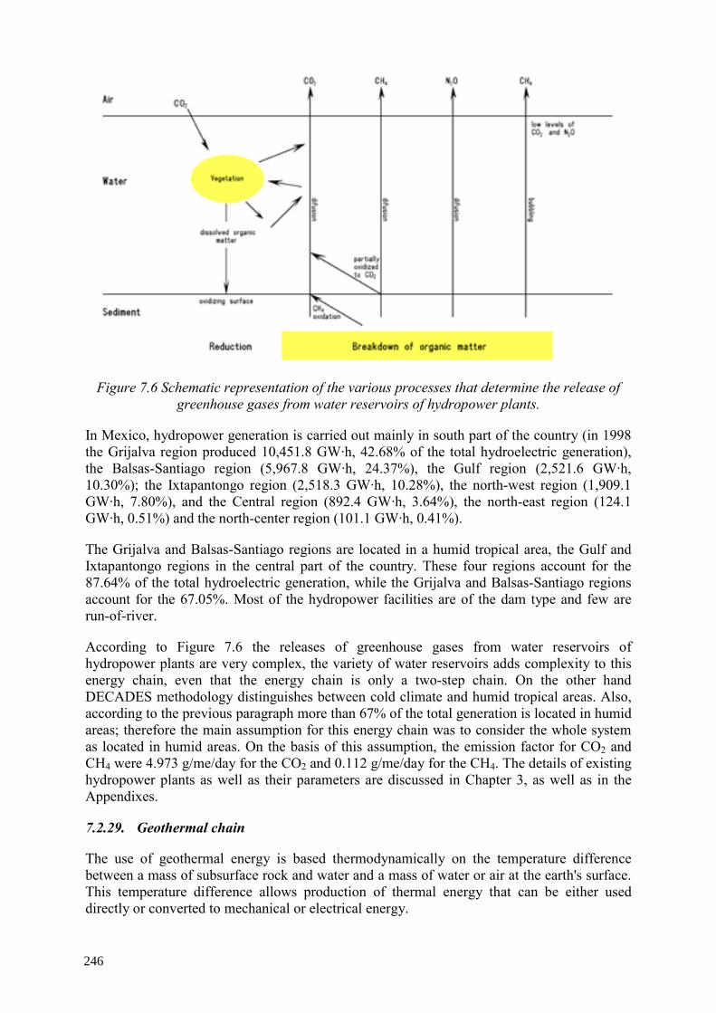
Figure 7.6 Schematic representation of the various processes that determine the release of greenhouse gases from water reservoirs of hydropower plants.

In Mexico, hydropower generation is carried out mainly in south part of the country (in 1998 the Grijalva region produced 10,451.8 GW·h, 42.68% of the total hydroelectric generation), the Balsas-Santiago region (5,967.8 GW·h, 24.37%), the Gulf region (2,521.6 GW·h, 10.30%); the Ixtapantongo region (2,518.3 GW·h, 10.28%), the north-west region (1,909.1 GW·h, 7.80%), and the Central region (892.4 GW·h, 3.64%), the north-east region (124.1 GW·h, 0.51%) and the north-center region (101.1 GW·h, 0.41%).

The Grijalva and Balsas-Santiago regions are located in a humid tropical area, the Gulf and Ixtapantongo regions in the central part of the country. These four regions account for the 87.64% of the total hydroelectric generation, while the Grijalva and Balsas-Santiago regions account for the 67.05%. Most of the hydropower facilities are of the dam type and few are run-of-river.

According to Figure 7.6 the releases of greenhouse gases from water reservoirs of hydropower plants are very complex, the variety of water reservoirs adds complexity to this energy chain, even that the energy chain is only a two-step chain. On the other hand DECADES methodology distinguishes between cold climate and humid tropical areas. Also, according to the previous paragraph more than 67% of the total generation is located in humid areas; therefore the main assumption for this energy chain was to consider the whole system as located in humid areas. On the basis of this assumption, the emission factor for CO2 and CH4 were 4.973 g/me/day for the CO2 and 0.112 g/me/day for the CH4. The details of existing hydropower plants as well as their parameters are discussed in Chapter 3, as well as in the Appendixes.

7.2.29. Geothermal chain

The use of geothermal energy is based thermodynamically on the temperature difference between a mass of subsurface rock and water and a mass of water or air at the earth's surface. This temperature difference allows production of thermal energy that can be either used directly or converted to mechanical or electrical energy.

246

Temperatures in the earth in general increase with increasing depth, to 200 –1 000 ºC at the base of the Earth's crust and to perhaps 3 500 – 4 500 ºC at the center of the earth. The heat produces geothermal gradients and this heat comes from two sources: flow of heat from the deep crust and mantle; and thermal energy generated in the upper crust by radioactive decay of isotopes of uranium, thorium, and potassium. Some granite rocks in the upper crust, however, has abnormally high contents of uranium and Thorium and thus produce anomalously great amounts of thermal energy and enhanced flow of heat toward the earth surface. Consequently, thermal gradients at shallow levels above these granite plutons can be somehow higher.

These thermal gradients can be calculated under the assumption that heat moves toward the earth surface only by thermal conduction through the solid rock. However, thermal energy is also transmitted toward the earth surface by movement of the molten rock (magma) and by circulation of water through interconnected pores and fractures. These processes are superimposed and give rise to very high temperatures near the earth surface. Areas characterized by such high temperatures are the primary targets for geothermal exploration and development.

Commercial exploration and development of geothermal energy have focused on natural geothermal reservoirs - volumes of rock at high temperature and with both high porosity (pore space, usually filled with water) and high permeability (ability to transmit fluid). The thermal energy is tapped by drilling well into the reservoirs. The thermal energy in the rock is transferred by conduction to the fluid, which subsequently flows to the well and then to the earth surface.

Natural geothermal reservoirs, however, make up only a small fraction of the upper part of the earth crust. The remainder is rock of relatively low permeability whose thermal energy cannot be produced without fracturing the rock artificially by means of explosives or hydro fracturing. There are several types of natural geothermal reservoirs. Most of the reservoirs developed to date for electrical energy are termed hydrothermal convection systems and are characterized by circulation of meteoric (surface) water to depth. The driving force of the convection systems is gravity, effective because of the density difference between cold, downward moving, recharge water and heated, upward-moving, thermal water.

A hydrothermal convection system can be driven either by an underlying young igneous intrusion or by merely deep circulation of water along faults and fractures. Depending on the physical state of the pore fluid, there are two kinds of hydrothermal convection systems: liquid -dominated, in which all the pores and fractures are filled with liquid water that exists at temperatures well above boiling at atmospheric pressure, owing to the pressure of overlying water; and vapor-dominated, in which the larger pores and fractures are filled with steam. Liquid-dominated reservoirs produce either water or a mixture of water and steam, whereas vapor -dominated reservoirs produce only steam, in most cases superheated.

In some rapidly subsiding young sedimentary basins such as the northern Gulf of Mexico Basin, porous reservoir sandstones are compartmentalized by growth faults into individual reservoirs that can have fluid pressures exceeding that of a column of water and approaching that of the overlying rock. The pore water is prevented from escaping by the impermeable shale that surrounds the compartmented sandstone. The energy of these geopressured reservoirs consists not only of thermal energy, but also of an equal amount of energy from methane dissolved in the waters plus a small amount of mechanical energy due to the high fluid pressures.

247

Although geothermal energy is present everywhere beneath the earth's surface, its use is possible when certain conditions are met:

• The energy must be accessible to drilling, usually at depths of 3 000 meters (6 to 7 km under particularly favorable environments, such as is the case of the northern Gulf of Mexico Basin);

• Pending demonstration of the technology and economics for fracturing and producing energy from rock of low permeability, the reservoir porosity and permeability must be sufficiently high to allow production of large quantities of thermal water;

• Since the major cost in geothermal development is drilling and since cost per meter increase with increasing depth, the shallower the concentration of geothermal energy the better; and

• Geothermal fluids can be transported economically by pipeline on the earth's surface only a few tens of kilometers, and thus any generating or direct-use facility must be located at or near the geothermal anomaly.

The most conspicuous use of geothermal energy is the generation of electricity. Hot water from the liquid-dominated reservoir is flashed partly to steam in the earth's surface, and this steam is used to drive a conventional turbine-generator set. In the relatively rare vapor-dominated reservoirs, superheated steam produced by wells can be piped directly to the turbine without need for separation of water. Electricity is most readily produced from reservoirs of 180ºC or greater, but reservoirs of 150ºC or even lower show promise for electrical generation, either by using steam directly or by transferring its heat to a working fluid of low boiling point such as isobutene or freon. Besides electric generation, there are direct uses such as heating and cooling of buildings, to provide hot or warm water for domestic use, for product processing, and many other possible uses.

In any analysis of the possible contribution of geothermal energy to human energy needs, one must keep in mind that the geothermal resource is only a fraction of the thermal energy in the subsurface volume of rock and water. For favorable hydrothermal convection systems, this fraction can be 25% or greater, but for systems of restricted permeability the fraction is likely to be far smaller. Only this recoverable energy can be meaningfully compared with the thermal energy equivalent of barrels of recoverable oil, cubic meters of recoverable gas, tons of minable coal, or kilograms of minable uranium.

The main environmental problems in producing geothermal power involve mineral deposition, changes in hydrological conditions, and corrosion of equipment. Pollution problems arise in handling geothermal effluents both water and steam. Geothermal energy may have adverse environmental effects on air, water, and land. The exact effects are site-specific varying according to the properties of the reservoir and the plant design.

Air pollutants are emitted through direct releases of geothermal steam and through releases of non-condensable gases. The type and quantity of pollutants are site-specific and they will depend on the chemical composition of the geothermal fluid. In some water-dominated fields there may be mineral deposition from boiling geothermal fluid. Silica deposition in wells can cause problems. Calcium carbonate scale formation in wells or in the country rock may limit field development.

248

Extensive production from wells changes the local hydrological conditions. Decreasing aquifer pressures may cause boiling of the water in the rocks (leading to changes in well fluid characteristics), encroachment of cool water from the outskirts of the field, or changes in water chemistry through lowered temperatures and gas concentrations. After an extensive withdrawal of hot water from the rocks of low strength, localized ground subsidence may occur and the original natural thermal activity may diminish in intensity. Land subsidence appears to be a problem, but mainly in liquid-dominated geothermal fields.

In the case of vapor-dominated geothermal fields, subsidence does not appear to be problem, because the formation of these fields requires the presence of a rock that is not subject to compaction and subsidence. Anyway, some changes occur in all fields, and a good understanding of the geology and hydrology of a system is needed so that the well withdrawal rate can be matched to the well's long term capacity to supply fluid.

Geothermal waters cause an accelerated corrosion of most metal alloys, but this is not a serious utilization problem except in areas where wells tap high-temperature acid waters. The usual deep geothermal water is of near neutral pH. The principal metal corrosion effects to be avoided are sulfide and chloride stress corrosion of certain stainless and high-strength steels and the rapid corrosion of cooper-based alloys. Hydrogen sulfide, or its oxidation products, also causes a more rapid degradation than normal of building materials, such as concrete, plastics and paints.

Geothermal steam suppliers differ widely in gas content. The gas is predominantly carbon dioxide, hydrogen sulfide, methane, and ammonia. Hydrogen sulfide (H2S) is the air effluent of the biggest concern as it is highly toxic. Its direct effect on humans ranges from noxious odor at lower concentrations through systemic symptoms and death at higher concentrations and relatively short exposure time. In the case of geothermal energy, H2S concentrations are usually below toxic levels, but H2S is a problem because its odor and chemical reactivity. Implications of this may include corrosion of metals, blackening of paints, and vegetation damage. It therefore may then require control in specific cases.

CO2 effluents do not create environmental problems near the plant, but may make a contribution to global atmospheric build-up of CO2. Some estimates indicate that the contribution can be of a similar magnitude to that from a coal-fired plant. According to the UNEP27, in the case of Cerro Prieto's power plant the amount of CO2 could be of 150 000 ton per year on the basis of a 100 MW plant.

Ammonia (NH3) creates no problem by itself because atmospheric processes to acceptable levels rapidly diffuse it. However, if NH3 reacts with other chemicals, it can cause harmful environmental impacts; for example, ammonia may react with H2S to form ammonium sulphate, which is harmful to the environment. Site-specific conditions may require some form of control.

Radon-222 is found in trace-amounts in the non-condensable gas portion of geothermal steam. However, radon has not been found to be a problem at geothermal plants. Nevertheless, it is necessary to study its effects when dispersed. Same situation appears to be in the case of mercury in geothermal steam, which is finally released into the atmosphere, but the concentrations created have to be studied.

27 UNEP, The Environmental Impacts of Production and Use of Energy, Part III: Renewable Sources of Energy, Nairobi, August 1980.

249

The compositions of geothermal waters vary widely. Those in recent volcanic areas are commonly dilute saline solutions, but waters in sedimentary basins or active volcanic areas range upward to concentrated brines. Most geothermal hot waters contain a relatively large amount of dissolved solids and heavy metals. Usually, geothermal water is sodium, potassium chloride solution containing relatively large concentrations of some elements and metals. In comparison with surface waters, most geothermal waters contain exceptional concentrations of boron, fluoride, ammonia, silica, hydrogen sulfide, and arsenic. In the common dilute geothermal waters, the concentrations of heavy metals such as iron, manganese, lead, zinc, cadmium, and thallium seldom exceed the levels permissible in drinking waters. However, the concentrated brines may contain appreciable levels of heavy metals.

Because of their composition, effluent geothermal waters or condensates may adversely affect potable or irrigation water supplies and aquatic life. Ammonia can increase weed growth in waterways and promote eutrophication, while the entry of boron to irrigation waters may affect sensitive plants such as citrus. Small quantities of metal sulfide precipitate from waters, containing arsenic, antimony, and mercury, can accumulate in stream sediments and cause fish to derive undesirably high mercury concentrations.

The following methods could be used for disposing the waste of waste water: direct release to surface water bodies, evaporation, surface spreading to shallow aquifers, desalination with subsequent water reuse, and re-injection to the reservoir. The exact disposal method depends on local hydrologic conditions, water requirements, and environmental regulations. In the case of re-injection, steam condensate re-injection seem to have few problems, but the case of much larger volumes of separate waste hot water from water-dominated fields present a more difficult re-injection situation.

Silica and carbonate deposition may cause blockages in the rock fissures if appropriate temperature, chemical, and hydrological regimes are not met at the disposal depth. In some cases, chemical processing of the brines may be necessary before re-injection. Selective re-injection of water into the thermal system may help to retain aquifer pressures and to extract further heat from the rock. Dissolved silica may create problems, because if it enters the wastewater channels, the latter have to clean regularly.

For example, the water from Cerro Prieto's power plant contains, approximately, the same quantity of silica than Los Azufres power plant, six times more chloride, potassium and sodium. On the other hand Los Azufres presents more than 200 ppm of boron and 20 ppm of arsenic.

These considerations induce to recognize that the water deposition method will be different from one place to another. In Cerro Prieto's power plant is possible to dispose of the wastewater in evaporation ponds since the power plant is located at a desert area. This is not the case of Los Azufres since the climate and orography would prevent this possibility.

Noise could be another problem with geothermal energy, since noise levels could reach 120 decibels in the vicinity of unsilenced geothermal wells. Silencers could reduce the noise level to below 100 decibels and remove the high frequencies. Uncontrolled wells may produce ground vibrations and secondary drilling may be required to stop these vibrations.

Finally, the amount of land required for the development of a geothermal field depends on the topography and the well density. In geothermal plants with a low efficiency the waste heat discharge may create problems, such as local fog formation and icing of roads during winter.

250

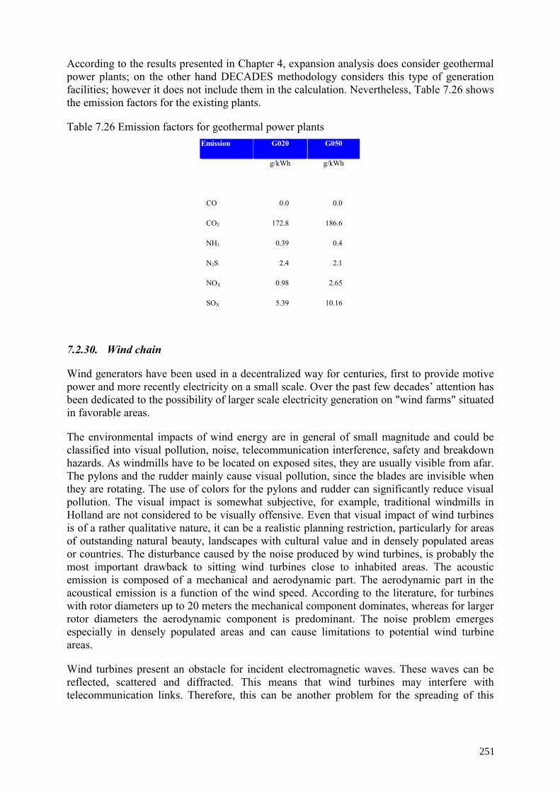
According to the results presented in Chapter 4, expansion analysis does consider geothermal power plants; on the other hand DECADES methodology considers this type of generation facilities; however it does not include them in the calculation. Nevertheless, Table 7.26 shows the emission factors for the existing plants.

Table 7.26 Emission factors for geothermal power plants Emission G020 G050

g/kWh g/kWh

CO 0.0 0.0

CO2 172.8 186.6

NH3 0.39 0.4

N2S 2.4 2.1

NOX 0.98 2.65

SOX 5.39 10.16

7.2.30. Wind chain

Wind generators have been used in a decentralized way for centuries, first to provide motive power and more recently electricity on a small scale. Over the past few decades’ attention has been dedicated to the possibility of larger scale electricity generation on "wind farms" situated in favorable areas.

The environmental impacts of wind energy are in general of small magnitude and could be classified into visual pollution, noise, telecommunication interference, safety and breakdown hazards. As windmills have to be located on exposed sites, they are usually visible from afar. The pylons and the rudder mainly cause visual pollution, since the blades are invisible when they are rotating. The use of colors for the pylons and rudder can significantly reduce visual pollution. The visual impact is somewhat subjective, for example, traditional windmills in Holland are not considered to be visually offensive. Even that visual impact of wind turbines is of a rather qualitative nature, it can be a realistic planning restriction, particularly for areas of outstanding natural beauty, landscapes with cultural value and in densely populated areas or countries. The disturbance caused by the noise produced by wind turbines, is probably the most important drawback to sitting wind turbines close to inhabited areas. The acoustic emission is composed of a mechanical and aerodynamic part. The aerodynamic part in the acoustical emission is a function of the wind speed. According to the literature, for turbines with rotor diameters up to 20 meters the mechanical component dominates, whereas for larger rotor diameters the aerodynamic component is predominant. The noise problem emerges especially in densely populated areas and can cause limitations to potential wind turbine areas.

Wind turbines present an obstacle for incident electromagnetic waves. These waves can be reflected, scattered and diffracted. This means that wind turbines may interfere with telecommunication links. Therefore, this can be another problem for the spreading of this

251

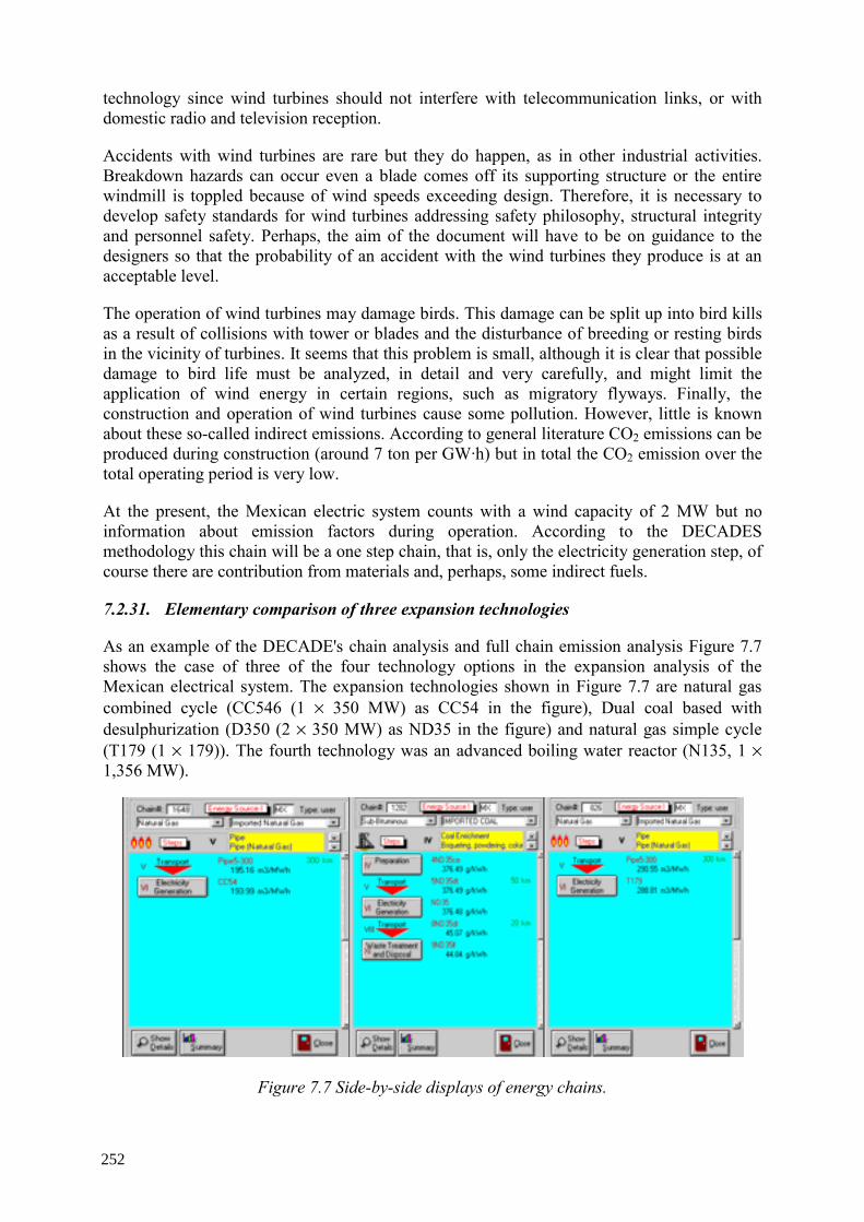
technology since wind turbines should not interfere with telecommunication links, or with domestic radio and television reception.

Accidents with wind turbines are rare but they do happen, as in other industrial activities. Breakdown hazards can occur even a blade comes off its supporting structure or the entire windmill is toppled because of wind speeds exceeding design. Therefore, it is necessary to develop safety standards for wind turbines addressing safety philosophy, structural integrity and personnel safety. Perhaps, the aim of the document will have to be on guidance to the designers so that the probability of an accident with the wind turbines they produce is at an acceptable level.

The operation of wind turbines may damage birds. This damage can be split up into bird kills as a result of collisions with tower or blades and the disturbance of breeding or resting birds in the vicinity of turbines. It seems that this problem is small, although it is clear that possible damage to bird life must be analyzed, in detail and very carefully, and might limit the application of wind energy in certain regions, such as migratory flyways. Finally, the construction and operation of wind turbines cause some pollution. However, little is known about these so-called indirect emissions. According to general literature CO2 emissions can be produced during construction (around 7 ton per GW·h) but in total the CO2 emission over the total operating period is very low.

At the present, the Mexican electric system counts with a wind capacity of 2 MW but no information about emission factors during operation. According to the DECADES methodology this chain will be a one step chain, that is, only the electricity generation step, of course there are contribution from materials and, perhaps, some indirect fuels.

7.2.31. Elementary comparison of three expansion technologies

As an example of the DECADE's chain analysis and full chain emission analysis Figure 7.7 shows the case of three of the four technology options in the expansion analysis of the Mexican electrical system. The expansion technologies shown in Figure 7.7 are natural gas combined cycle (CC546 (1 × 350 MW) as CC54 in the figure), Dual coal based with desulphurization (D350 (2 × 350 MW) as ND35 in the figure) and natural gas simple cycle (T179 (1 × 179)). The fourth technology was an advanced boiling water reactor (N135, 1 × 1,356 MW).

Figure 7.7 Side-by-side displays of energy chains.

252

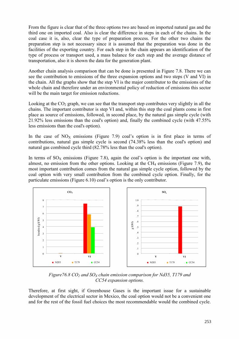
From the figure is clear that of the three options two are based on imported natural gas and the third one on imported coal. Also is clear the difference in steps in each of the chains. In the coal case it is, also, clear the type of preparation process. For the other two chains the preparation step is not necessary since it is assumed that the preparation was done in the facilities of the exporting country. For each step in the chain appears an identification of the type of process or transport used, a mass balance for each step and the average distance of transportation, also it is shown the data for the generation plant.

Another chain analysis comparison that can be done is presented in Figure 7.8. There we can see the contribution to emissions of the three expansion options and two steps (V and VI) in the chain. All the graphs show that the step VI is the major contributor to the emissions of the whole chain and therefore under an environmental policy of reduction of emissions this sector will be the main target for emission reductions.

Looking at the CO2 graph, we can see that the transport step contributes very slightly in all the chains. The important contributor is step VI and, within this step the coal plants come in first place as source of emissions, followed, in second place, by the natural gas simple cycle (with 21.92% less emissions than the coal's option) and, finally the combined cycle (with 47.55% less emissions than the coal's option).

In the case of NOX emissions (Figure 7.9) coal’s option is in first place in terms of contributions, natural gas simple cycle is second (74.38% less than the coal's option) and natural gas combined cycle third (82.78% less than the coal's option).

In terms of SOX emissions (Figure 7.8), again the coal’s option is the important one with, almost, no emission from the other options. Looking at the CH4 emissions (Figure 7.9), the most important contribution comes from the natural gas simple cycle option, followed by the coal option with very small contribution from the combined cycle option. Finally, for the particulate emissions (Figure 6.10) coal’s option is the only contributor.

CO2

0

1

2

3

4

5

6

7

8

V VI

hund

red

g/kW

h

ND35 T179 CC54

SOx

0

.1

.2

.3

.4

.5

.6

.7

.8

.9

1.0

V VI

g/kW

h

ND35 T179 CC54

Figure76.8 CO2 and SOX chain emission comparison for Nd35, T179 and CC54 expansion options.

Therefore, at first sight, if Greenhouse Gases is the important issue for a sustainable development of the electrical sector in Mexico, the coal option would not be a convenient one and for the rest of the fossil fuel choices the most recommendable would the combined cycle.

253

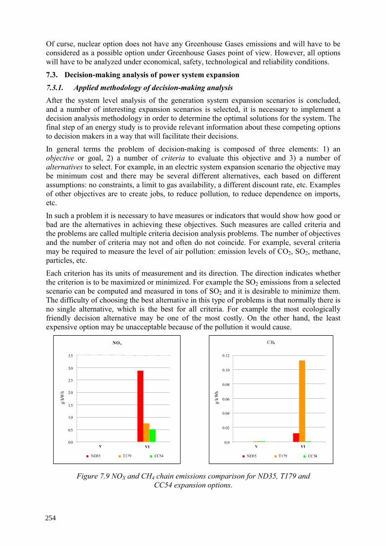
Of curse, nuclear option does not have any Greenhouse Gases emissions and will have to be considered as a possible option under Greenhouse Gases point of view. However, all options will have to be analyzed under economical, safety, technological and reliability conditions.

7.3. Decision-making analysis of power system expansion

7.3.1. Applied methodology of decision-making analysis After the system level analysis of the generation system expansion scenarios is concluded, and a number of interesting expansion scenarios is selected, it is necessary to implement a decision analysis methodology in order to determine the optimal solutions for the system. The final step of an energy study is to provide relevant information about these competing options to decision makers in a way that will facilitate their decisions.

In general terms the problem of decision-making is composed of three elements: 1) an objective or goal, 2) a number of criteria to evaluate this objective and 3) a number of alternatives to select. For example, in an electric system expansion scenario the objective may be minimum cost and there may be several different alternatives, each based on different assumptions: no constraints, a limit to gas availability, a different discount rate, etc. Examples of other objectives are to create jobs, to reduce pollution, to reduce dependence on imports, etc.

In such a problem it is necessary to have measures or indicators that would show how good or bad are the alternatives in achieving these objectives. Such measures are called criteria and the problems are called multiple criteria decision analysis problems. The number of objectives and the number of criteria may not and often do not coincide. For example, several criteria may be required to measure the level of air pollution: emission levels of CO2, SO2, methane, particles, etc.

Each criterion has its units of measurement and its direction. The direction indicates whether the criterion is to be maximized or minimized. For example the SO2 emissions from a selected scenario can be computed and measured in tons of SO2 and it is desirable to minimize them. The difficulty of choosing the best alternative in this type of problems is that normally there is no single alternative, which is the best for all criteria. For example the most ecologically friendly decision alternative may be one of the most costly. On the other hand, the least expensive option may be unacceptable because of the pollution it would cause.

NOx

0.0

0.5

1.0

1.5

2.0

2.5

3.0

3.5

V VI

g/kW

h

ND35 T179 CC54

CH4

0.0

0.02

0.04

0.06

0.08

0.10

0.12

V VI

g/kW

h

ND35 T179 CC54

Figure 7.9 NOX and CH4 chain emissions comparison for ND35, T179 and CC54 expansion options.

254

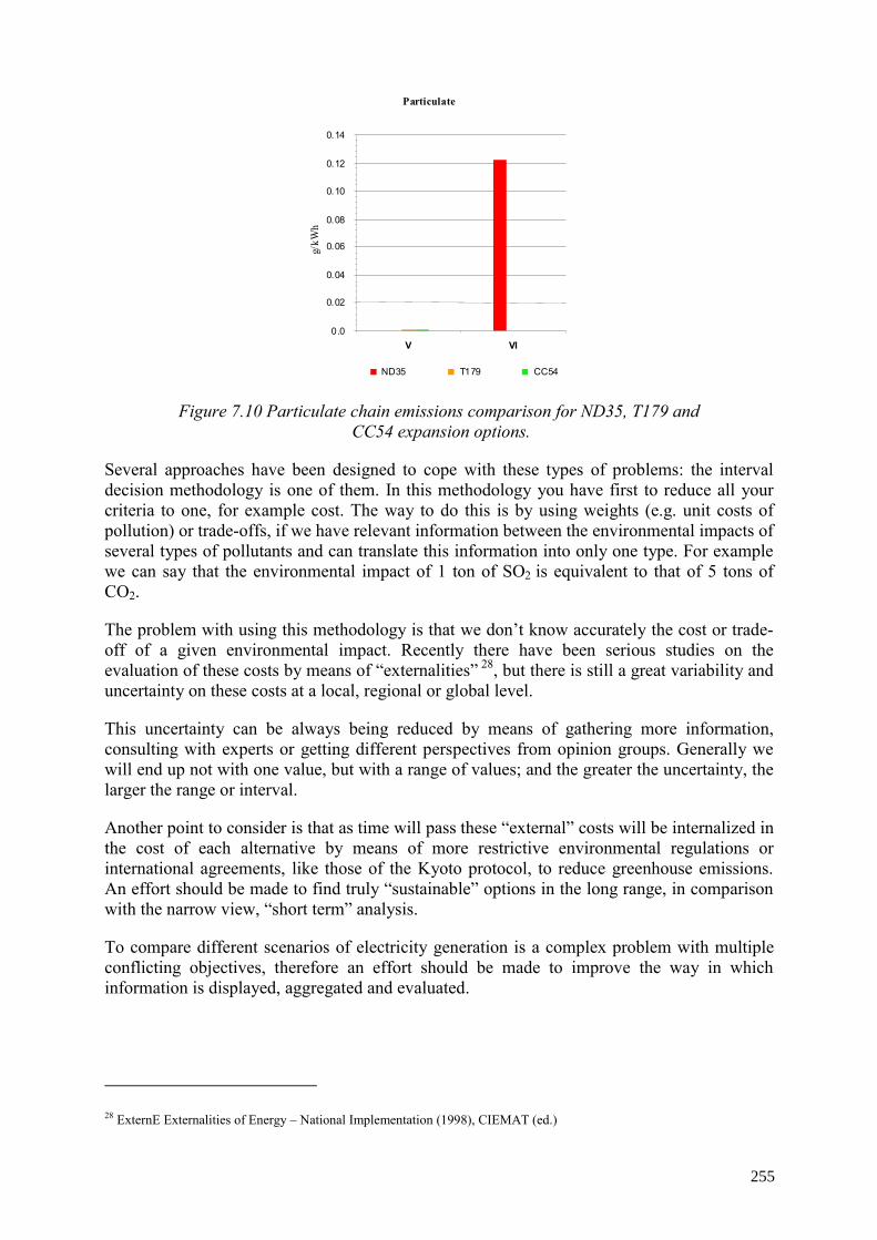
Particulate

0.0

0.02

0.04

0.06

0.08

0.10

0.12

0.14

V VI

ND35 T179 CC54

g/kW

h

Figure 7.10 Particulate chain emissions comparison for ND35, T179 and CC54 expansion options.

Several approaches have been designed to cope with these types of problems: the interval decision methodology is one of them. In this methodology you have first to reduce all your criteria to one, for example cost. The way to do this is by using weights (e.g. unit costs of pollution) or trade-offs, if we have relevant information between the environmental impacts of several types of pollutants and can translate this information into only one type. For example we can say that the environmental impact of 1 ton of SO2 is equivalent to that of 5 tons of CO2.

The problem with using this methodology is that we don’t know accurately the cost or trade-off of a given environmental impact. Recently there have been serious studies on the evaluation of these costs by means of “externalities” 28, but there is still a great variability and uncertainty on these costs at a local, regional or global level.

This uncertainty can be always being reduced by means of gathering more information, consulting with experts or getting different perspectives from opinion groups. Generally we will end up not with one value, but with a range of values; and the greater the uncertainty, the larger the range or interval.

Another point to consider is that as time will pass these “external” costs will be internalized in the cost of each alternative by means of more restrictive environmental regulations or international agreements, like those of the Kyoto protocol, to reduce greenhouse emissions. An effort should be made to find truly “sustainable” options in the long range, in comparison with the narrow view, “short term” analysis.

To compare different scenarios of electricity generation is a complex problem with multiple conflicting objectives, therefore an effort should be made to improve the way in which information is displayed, aggregated and evaluated.

28 ExternE Externalities of Energy – National Implementation (1998), CIEMAT (ed.)

255

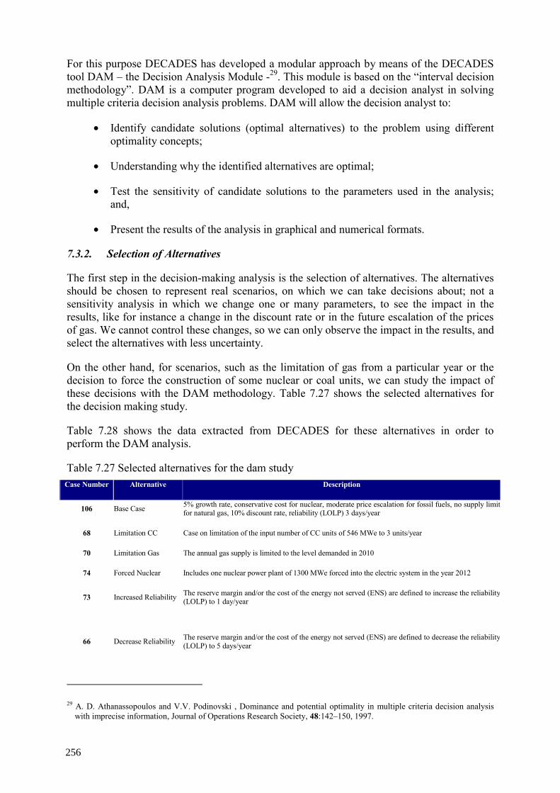
For this purpose DECADES has developed a modular approach by means of the DECADES tool DAM – the Decision Analysis Module -29. This module is based on the “interval decision methodology”. DAM is a computer program developed to aid a decision analyst in solving multiple criteria decision analysis problems. DAM will allow the decision analyst to:

• Identify candidate solutions (optimal alternatives) to the problem using different optimality concepts;

• Understanding why the identified alternatives are optimal;

• Test the sensitivity of candidate solutions to the parameters used in the analysis; and,

• Present the results of the analysis in graphical and numerical formats.

7.3.2. Selection of Alternatives

The first step in the decision-making analysis is the selection of alternatives. The alternatives should be chosen to represent real scenarios, on which we can take decisions about; not a sensitivity analysis in which we change one or many parameters, to see the impact in the results, like for instance a change in the discount rate or in the future escalation of the prices of gas. We cannot control these changes, so we can only observe the impact in the results, and select the alternatives with less uncertainty.

On the other hand, for scenarios, such as the limitation of gas from a particular year or the decision to force the construction of some nuclear or coal units, we can study the impact of these decisions with the DAM methodology. Table 7.27 shows the selected alternatives for the decision making study.

Table 7.28 shows the data extracted from DECADES for these alternatives in order to perform the DAM analysis.

Table 7.27 Selected alternatives for the dam study Case Number Alternative Description

106 Base Case 5% growth rate, conservative cost for nuclear, moderate price escalation for fossil fuels, no supply limitfor natural gas, 10% discount rate, reliability (LOLP) 3 days/year

68 Limitation CC Case on limitation of the input number of CC units of 546 MWe to 3 units/year

70 Limitation Gas The annual gas supply is limited to the level demanded in 2010

74 Forced Nuclear Includes one nuclear power plant of 1300 MWe forced into the electric system in the year 2012

73 Increased Reliability The reserve margin and/or the cost of the energy not served (ENS) are defined to increase the reliability(LOLP) to 1 day/year

66 Decrease Reliability The reserve margin and/or the cost of the energy not served (ENS) are defined to decrease the reliability(LOLP) to 5 days/year

29 A. D. Athanassopoulos and V.V. Podinovski , Dominance and potential optimality in multiple criteria decision analysis

with imprecise information, Journal of Operations Research Society, 48:142–150, 1997.

256

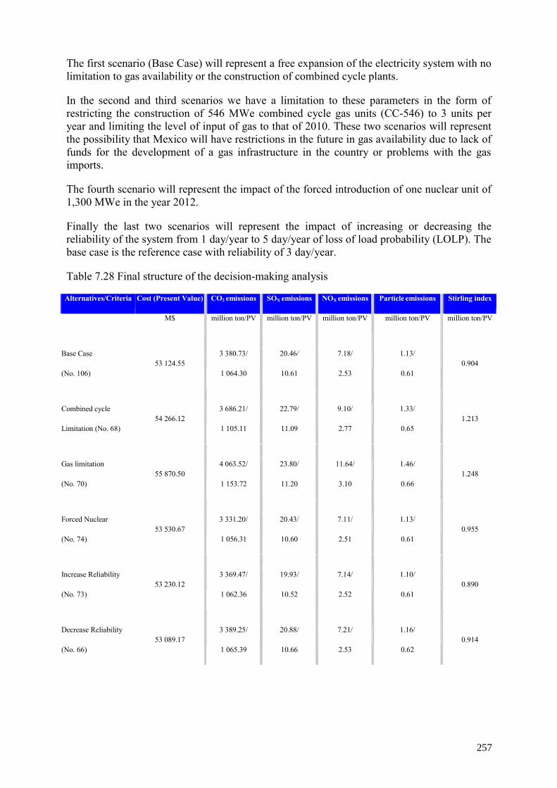
The first scenario (Base Case) will represent a free expansion of the electricity system with no limitation to gas availability or the construction of combined cycle plants.

In the second and third scenarios we have a limitation to these parameters in the form of restricting the construction of 546 MWe combined cycle gas units (CC-546) to 3 units per year and limiting the level of input of gas to that of 2010. These two scenarios will represent the possibility that Mexico will have restrictions in the future in gas availability due to lack of funds for the development of a gas infrastructure in the country or problems with the gas imports.

The fourth scenario will represent the impact of the forced introduction of one nuclear unit of 1,300 MWe in the year 2012.

Finally the last two scenarios will represent the impact of increasing or decreasing the reliability of the system from 1 day/year to 5 day/year of loss of load probability (LOLP). The base case is the reference case with reliability of 3 day/year.

Table 7.28 Final structure of the decision-making analysis

Alternatives/Criteria Cost (Present Value) CO2 emissions SOX emissions NOX emissions Particle emissions Stirling index

M$ million ton/PV million ton/PV million ton/PV million ton/PV million ton/PV

Base Case

(No. 106) 53 124.55

3 380.73/

1 064.30

20.46/

10.61

7.18/

2.53

1.13/

0.61

0.904

Combined cycle

Limitation (No. 68) 54 266.12

3 686.21/

1 105.11

22.79/

11.09

9.10/

2.77

1.33/

0.65

1.213

Gas limitation

(No. 70) 55 870.50

4 063.52/

1 153.72

23.80/

11.20

11.64/

3.10

1.46/

0.66

1.248

Forced Nuclear

(No. 74) 53 530.67

3 331.20/

1 056.31

20.43/

10.60

7.11/

2.51

1.13/

0.61

0.955

Increase Reliability

(No. 73) 53 230.12

3 369.47/

1 062.36

19.93/

10.52

7.14/

2.52

1.10/

0.61

0.890

Decrease Reliability

(No. 66) 53 089.17

3 389.25/

1 065.39

20.88/

10.66

7.21/

2.53

1.16/

0.62

0.914

257

These six scenarios will be compared from the point of view of cost, emissions and a third parameter called diversity index which will be explained as follows: we know the objective of the diversification of the system is among other things, to decrease the risk of a high volatility in the prices of fossil fuels such as gas, and its impact on cost. So to diversify our system, we have to introduce other fuels such as coal, nuclear or renewable energies, in order to have more stable overall prices.

A study carried out for Scottish Nuclear in September 199430, based in portfolio analysis, does implicitly predicts that competitive power markets provide less diversity. The study argues that it is advantageous for society to insure itself against the risk of price increases from fossil fuels by opting for diversity, and notably by using non-fossil, especially nuclear energy, as insurance.

So in the case of power plant investment decisions, the trade-off is made between low expected prices with a high level of uncertainty, and higher expected prices but with a lower level of uncertainty. The, adding of some higher-cost generating options act as an “insurance policy” against large price increases or “oil shocks” in fuel consumed in low cost plants.

A diversity index developed by Stirling31 was used to describe the diversity of the scenarios and was included in Table 7.28. The so-called Stirling index was used as an indicator of energy supply diversity. The index H was calculated for the mix of the capacity resulting in the final year of the study for the selected expansions using the formula:

)(pLnpH ii

i∑−=

where pi represents the proportion of installed capacity i in the total supply mix.

In order to define the value of one unit of this index for the DAM analysis, some methodologies were discussed. These methodologies can be based on the diversification obtained in the different scenarios, during the optimization of the expansions or in other methods like the direct calculation of the security externality or the estimated financial coverage of the gas prices. In the following section we will describe these methodologies.

7.3.3. Definition of criteria and criteria weights

In traditional methodologies, the environmental costs caused by pollutants are added to the economic costs required for the implementation of a decision alternative. The former are calculated by multiplying the levels of pollutants (e.g. in millions of tons) by the estimated unit damage costs of the pollutants (e.g. in US$ per ton).

An apparent weakness of this approach is that the unit damage costs have to be estimated precisely and this is clearly impossible because of the complexity of the task and the presence of uncertainty. To overcome this problem the unit damage costs may be varied and the decision analysis repeated a few times to test the sensitivity of the results to the assumed costs. However it is not often clear to what extent should the unit costs be varied and, more important, it is not possible to perform decision analysis for all feasible variations of the unit costs because there are infinitely many such variations.

30 Scottish Nuclear, “Diversity in UK Electricity Generation: A portfolio Analysis of the Contribution of Nuclear” ERM,

London, UK, 1994. 31 Stirling, A., “Diversity and Ignorance in Electricity Supply Investments”, Energy Policy, March 1994.

258

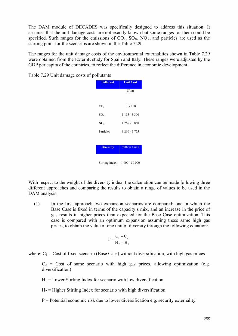
The DAM module of DECADES was specifically designed to address this situation. It assumes that the unit damage costs are not exactly known but some ranges for them could be specified. Such ranges for the emissions of CO2, SOX, NOX, and particles are used as the starting point for the scenarios are shown in the Table 7.29.

The ranges for the unit damage costs of the environmental externalities shown in Table 7.29 were obtained from the ExternE study for Spain and Italy. These ranges were adjusted by the GDP per capita of the countries, to reflect the difference in economic development.

Table 7.29 Unit damage costs of pollutants Pollutant Unit Cost

$/ton

CO2 18 - 100

SOx 1 155 - 3 300

NOx 1 265 - 3 850

Particles 1 210 - 5 775

Diversity million $/unit

Stirling Index 1 000 - 50 000

With respect to the weight of the diversity index, the calculation can be made following three different approaches and comparing the results to obtain a range of values to be used in the DAM analysis:

(1) In the first approach two expansion scenarios are compared: one in which the Base Case is fixed in terms of the capacity’s mix, and an increase in the price of gas results in higher prices than expected for the Base Case optimization. This case is compared with an optimum expansion assuming these same high gas prices, to obtain the value of one unit of diversity through the following equation:

12

21

HHCC

P−−

=

where: C1 = Cost of fixed scenario (Base Case) without diversification, with high gas prices

C2 = Cost of same scenario with high gas prices, allowing optimization (e.g. diversification)

H1 = Lower Stirling Index for scenario with low diversification

H2 = Higher Stirling Index for scenario with high diversification

P = Potential economic risk due to lower diversification e.g. security externality.

259

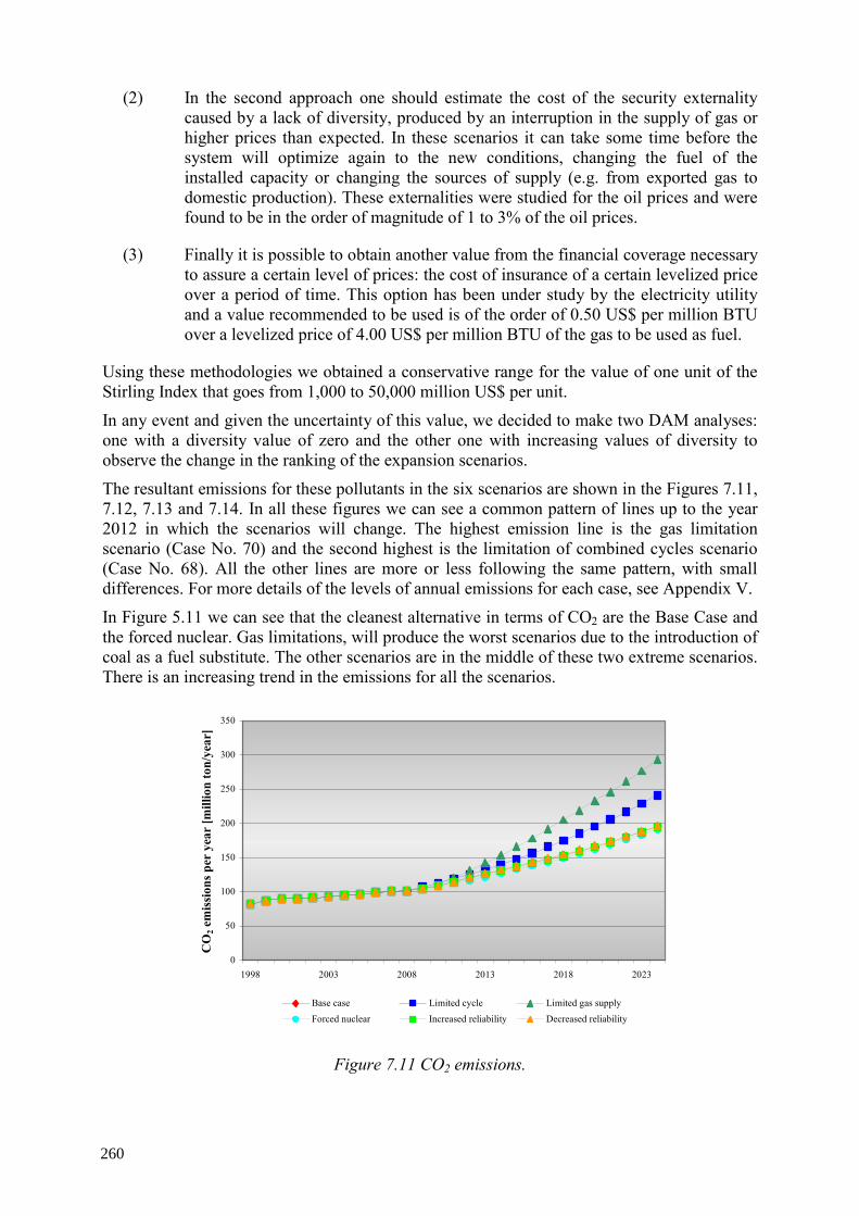
(2) In the second approach one should estimate the cost of the security externality caused by a lack of diversity, produced by an interruption in the supply of gas or higher prices than expected. In these scenarios it can take some time before the system will optimize again to the new conditions, changing the fuel of the installed capacity or changing the sources of supply (e.g. from exported gas to domestic production). These externalities were studied for the oil prices and were found to be in the order of magnitude of 1 to 3% of the oil prices.

(3) Finally it is possible to obtain another value from the financial coverage necessary to assure a certain level of prices: the cost of insurance of a certain levelized price over a period of time. This option has been under study by the electricity utility and a value recommended to be used is of the order of 0.50 US$ per million BTU over a levelized price of 4.00 US$ per million BTU of the gas to be used as fuel.

Using these methodologies we obtained a conservative range for the value of one unit of the Stirling Index that goes from 1,000 to 50,000 million US$ per unit.

In any event and given the uncertainty of this value, we decided to make two DAM analyses: one with a diversity value of zero and the other one with increasing values of diversity to observe the change in the ranking of the expansion scenarios.

The resultant emissions for these pollutants in the six scenarios are shown in the Figures 7.11, 7.12, 7.13 and 7.14. In all these figures we can see a common pattern of lines up to the year 2012 in which the scenarios will change. The highest emission line is the gas limitation scenario (Case No. 70) and the second highest is the limitation of combined cycles scenario (Case No. 68). All the other lines are more or less following the same pattern, with small differences. For more details of the levels of annual emissions for each case, see Appendix V.

In Figure 5.11 we can see that the cleanest alternative in terms of CO2 are the Base Case and the forced nuclear. Gas limitations, will produce the worst scenarios due to the introduction of coal as a fuel substitute. The other scenarios are in the middle of these two extreme scenarios. There is an increasing trend in the emissions for all the scenarios.

0

50

100

150

200

250

300

350

1998 2003 2008 2013 2018 2023

CO

2 em

issi

ons p

er y

ear

[mill

ion

ton/

year

]

Base case Limited cycle Limited gas supply

Forced nuclear Increased reliability Decreased reliability

Figure 7.11 CO2 emissions.

260

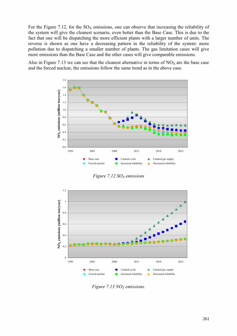
For the Figure 7.12, for the SOX emissions, one can observe that increasing the reliability of the system will give the cleanest scenario, even better than the Base Case. This is due to the fact that one will be dispatching the more efficient plants with a larger number of units. The reverse is shown as one have a decreasing pattern in the reliability of the system: more pollution due to dispatching a smaller number of plants. The gas limitation cases will give more emissions than the Base Case and the other cases will give comparable emissions.

Also in Figure 7.13 we can see that the cleanest alternative in terms of NOX are the base case and the forced nuclear, the emissions follow the same trend as in the above case.

0.0

0.2

0.4

0.6

0.8

1.0

1.2

1.4

1.6

1.8

1998 2003 2008 2013 2018 2023

SOX e

mis

sion

s [m

illio

n to

n/ye

ar]

Base case Limited cycle Limited gas supplyForced nuclear Increased reliability Decreased reliability

Figure 7.12 SOX emissions

0

0.2

0.4

0.6

0.8

1

1.2

1998 2003 2008 2013 2018 2023

NO

X e

mis

sion

s [m

illio

n to

n/ye

ar]

Base case Limited cycle Limited gas supplyForced nuclear Increased reliability Decreased reliability

Figure 7.13 NOX emissions.

261

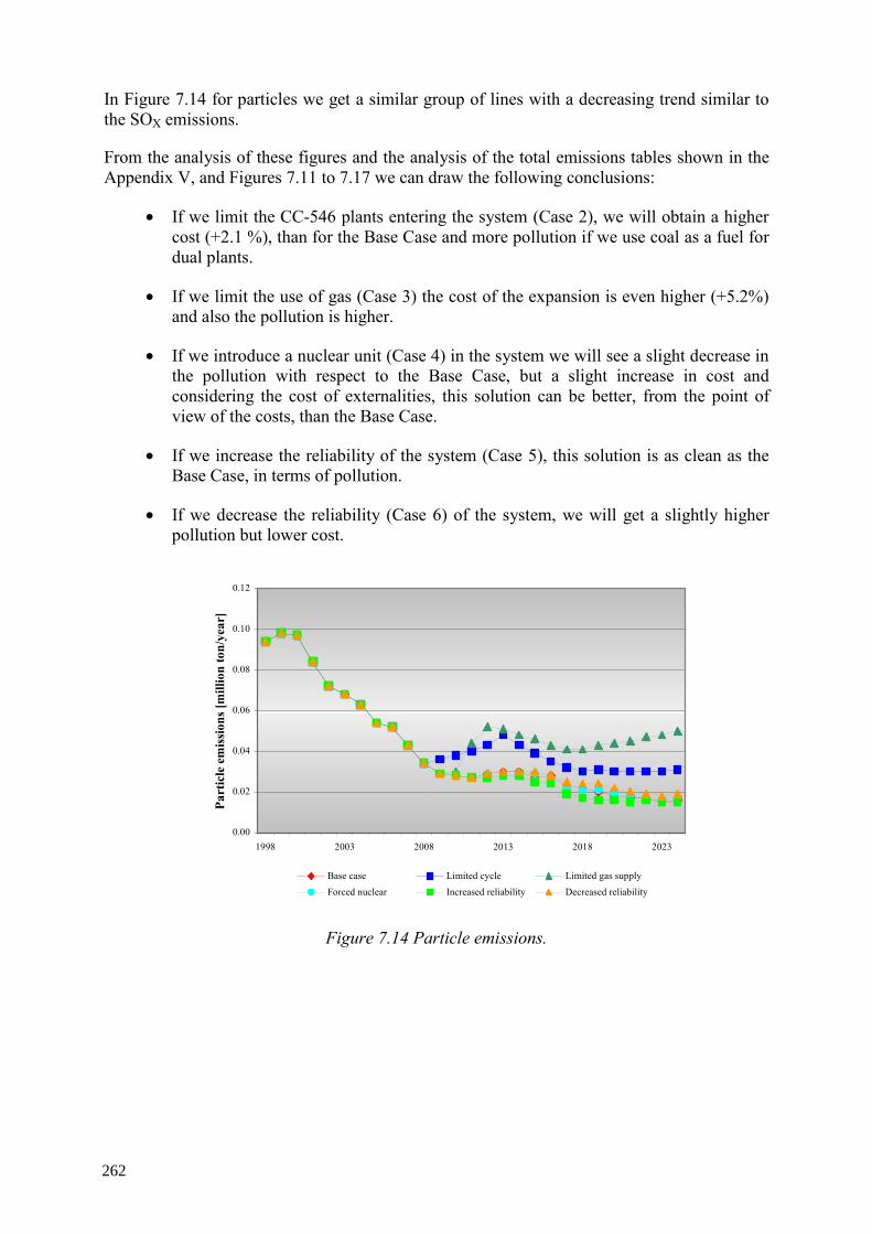
In Figure 7.14 for particles we get a similar group of lines with a decreasing trend similar to the SOX emissions.

From the analysis of these figures and the analysis of the total emissions tables shown in the Appendix V, and Figures 7.11 to 7.17 we can draw the following conclusions:

• If we limit the CC-546 plants entering the system (Case 2), we will obtain a higher cost (+2.1 %), than for the Base Case and more pollution if we use coal as a fuel for dual plants.

• If we limit the use of gas (Case 3) the cost of the expansion is even higher (+5.2%) and also the pollution is higher.

• If we introduce a nuclear unit (Case 4) in the system we will see a slight decrease in the pollution with respect to the Base Case, but a slight increase in cost and considering the cost of externalities, this solution can be better, from the point of view of the costs, than the Base Case.

• If we increase the reliability of the system (Case 5), this solution is as clean as the Base Case, in terms of pollution.

• If we decrease the reliability (Case 6) of the system, we will get a slightly higher pollution but lower cost.

0.00

0.02

0.04

0.06

0.08

0.10

0.12

1998 2003 2008 2013 2018 2023

Part

icle

em

issi

ons [

mill

ion

ton/

year

]

Base case Limited cycle Limited gas supply

Forced nuclear Increased reliability Decreased reliability

Figure 7.14 Particle emissions.

262

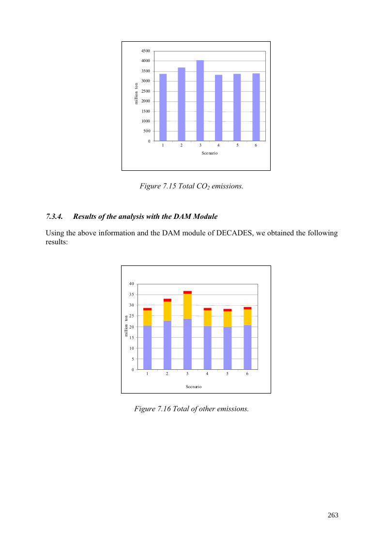
0

500

1000

1500

2000

2500

3000

3500

4000

4500

1 2 3 4 5 6

Scenario

mill

ion

ton

Figure 7.15 Total CO2 emissions.

7.3.4. Results of the analysis with the DAM Module

Using the above information and the DAM module of DECADES, we obtained the following results:

0

5

10

15

20

25

30

35

40

1 2 3 4 5 6

Scenario

mill

ion t

on

Figure 7.16 Total of other emissions.

263

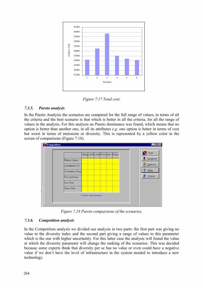
51500

52000

52500

53000

53500

54000

54500

55000

55500

56000

56500

1 2 3 4 5 6

Scenario

mill

ion

US$

Figure 7.17 Total cost.

7.3.5. Pareto analysis In the Pareto Analysis the scenarios are compared for the full range of values, in terms of all the criteria and the best scenario is that which is better in all the criteria, for all the range of values in the analysis. For this analysis no Pareto dominance was found, which means that no option is better than another one, in all its attributes e.g. one option is better in terms of cost but worst in terms of emissions or diversity. This is represented by a yellow color in the screen of comparisons (Figure 7.18).

Figure 7.18 Pareto comparisons of the scenarios.

7.3.6. Competition analysis

In the Competition analysis we divided our analysis in two parts: the first part was giving no value to the diversity index and the second part giving a range of values to this parameter which is the one with higher uncertainty. For this latter case the analysis will found the value at which the diversity parameter will change the ranking of the scenarios. This was decided because some experts think that diversity per se has no value or even could have a negative value if we don’t have the level of infrastructure in the system needed to introduce a new technology.

264

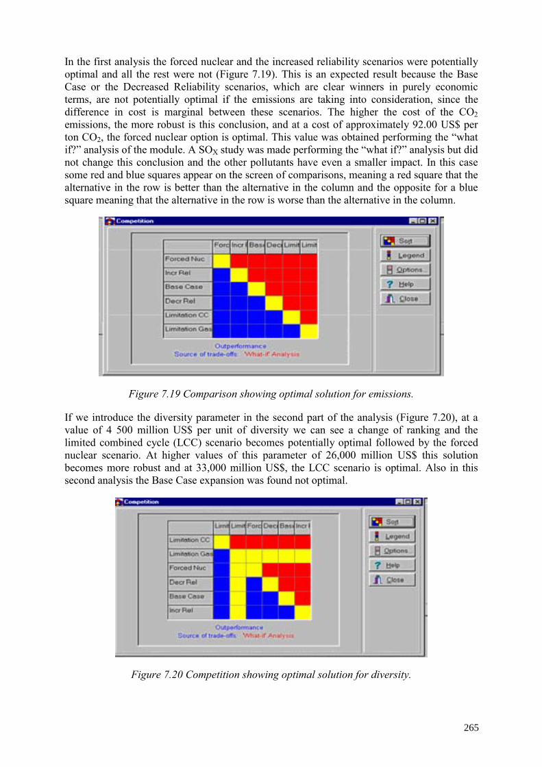
In the first analysis the forced nuclear and the increased reliability scenarios were potentially optimal and all the rest were not (Figure 7.19). This is an expected result because the Base Case or the Decreased Reliability scenarios, which are clear winners in purely economic terms, are not potentially optimal if the emissions are taking into consideration, since the difference in cost is marginal between these scenarios. The higher the cost of the CO2 emissions, the more robust is this conclusion, and at a cost of approximately 92.00 US$ per ton CO2, the forced nuclear option is optimal. This value was obtained performing the “what if?” analysis of the module. A SOX study was made performing the “what if?” analysis but did not change this conclusion and the other pollutants have even a smaller impact. In this case some red and blue squares appear on the screen of comparisons, meaning a red square that the alternative in the row is better than the alternative in the column and the opposite for a blue square meaning that the alternative in the row is worse than the alternative in the column.

Figure 7.19 Comparison showing optimal solution for emissions.

If we introduce the diversity parameter in the second part of the analysis (Figure 7.20), at a value of 4 500 million US$ per unit of diversity we can see a change of ranking and the limited combined cycle (LCC) scenario becomes potentially optimal followed by the forced nuclear scenario. At higher values of this parameter of 26,000 million US$ this solution becomes more robust and at 33,000 million US$, the LCC scenario is optimal. Also in this second analysis the Base Case expansion was found not optimal.

Figure 7.20 Competition showing optimal solution for diversity.

265

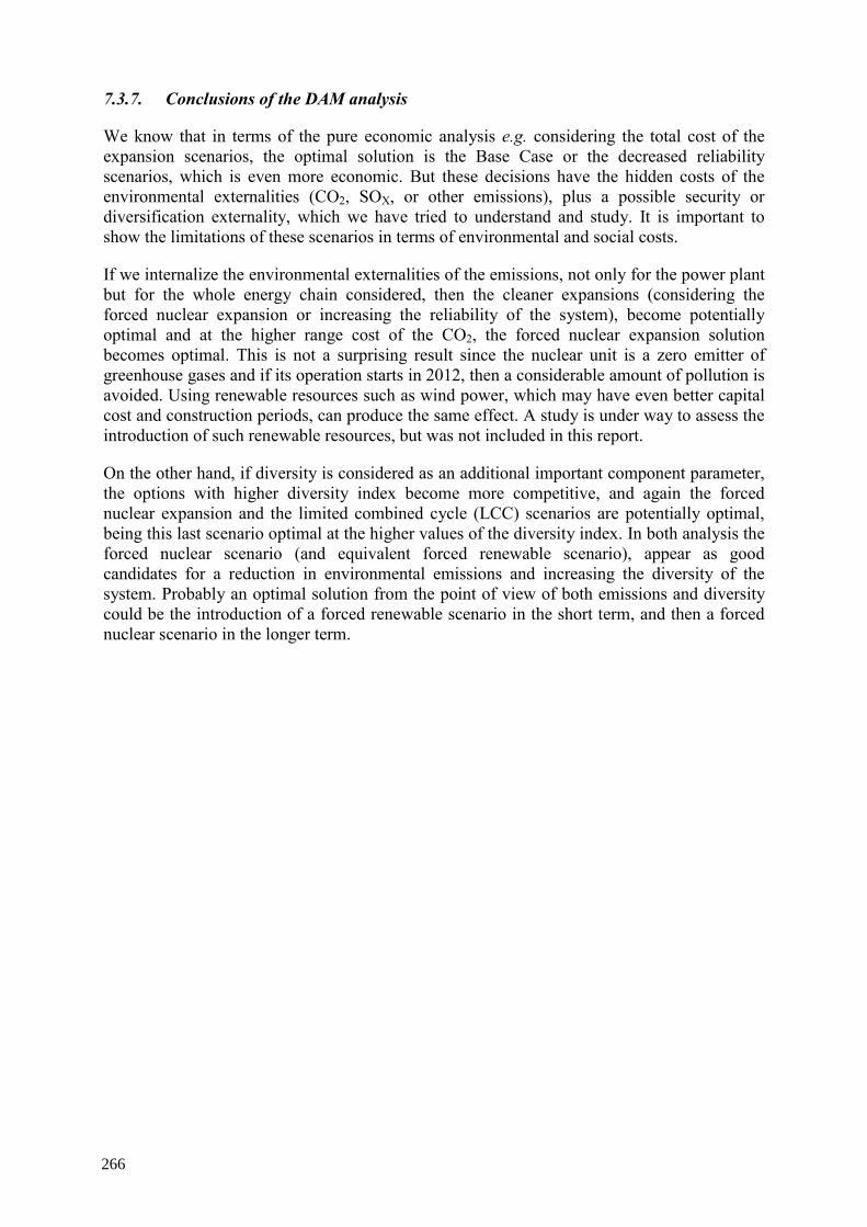
7.3.7. Conclusions of the DAM analysis

We know that in terms of the pure economic analysis e.g. considering the total cost of the expansion scenarios, the optimal solution is the Base Case or the decreased reliability scenarios, which is even more economic. But these decisions have the hidden costs of the environmental externalities (CO2, SOX, or other emissions), plus a possible security or diversification externality, which we have tried to understand and study. It is important to show the limitations of these scenarios in terms of environmental and social costs.

If we internalize the environmental externalities of the emissions, not only for the power plant but for the whole energy chain considered, then the cleaner expansions (considering the forced nuclear expansion or increasing the reliability of the system), become potentially optimal and at the higher range cost of the CO2, the forced nuclear expansion solution becomes optimal. This is not a surprising result since the nuclear unit is a zero emitter of greenhouse gases and if its operation starts in 2012, then a considerable amount of pollution is avoided. Using renewable resources such as wind power, which may have even better capital cost and construction periods, can produce the same effect. A study is under way to assess the introduction of such renewable resources, but was not included in this report.

On the other hand, if diversity is considered as an additional important component parameter, the options with higher diversity index become more competitive, and again the forced nuclear expansion and the limited combined cycle (LCC) scenarios are potentially optimal, being this last scenario optimal at the higher values of the diversity index. In both analysis the forced nuclear scenario (and equivalent forced renewable scenario), appear as good candidates for a reduction in environmental emissions and increasing the diversity of the system. Probably an optimal solution from the point of view of both emissions and diversity could be the introduction of a forced renewable scenario in the short term, and then a forced nuclear scenario in the longer term.

266

8. CONCLUSIONS

The first type of conclusions refers to the attainment of the objectives of the project. The country specific data base (CSDB) for Mexico was created; the initial screening of the candidate technologies for the electric system expansion was done in terms of their technical performance, economic competitiveness and environmental impacts; comparative assessment of full energy chains was the most difficult task of the project, but nevertheless was completed although with some delay due to the amount, detail and complexity of the data required; finally, the comparative assessment of electricity system expansion strategies until 2025 was successfully completed, with one base case and 14 alternatives considered.

The second type of conclusions is related to the usefulness of the tools supplied by the IAEA to the Government of Mexico and their use in future studies. Although CFE had for some years been using the WASP module for electric system expansion analysis, the supply of the DECADES package with the additional VALORAGUA and the DAM models has increased qualitatively the capacity for analysis of the hydro-thermal interaction and of the environmental impacts of the electrical generation system. Also SENER, IIE and UNAM have benefited from the availability and detailed knowledge of these tools because they can be used skillfully in further studies.

The third type of conclusions refers to the synthetic analysis of the main results of the system level expansion study and the DAM program. In this respect, the basic expansion of the interconnected system would be based on natural gas fired combined cycle units, with some gas turbines for peak demand hours. Nonetheless, the possibility of natural gas prices increases makes it desirable to consider some diversification using alternative technologies such as coal fired dual units, fuel oil units, and nuclear units. In such cases the total discounted costs can increase but a higher diversification is provided, the dependence on foreign fuel sources supply is reduced increasing the independence of this strategic sector. Moreover, some environmental benefits can be obtained as well, such as lower CO2 emissions in the case of nuclear units.

The fourth type of conclusions to be derived from the study is the need for SENER, CFE, IIE and UNAM to analyze with much more detail the issue of economic, environmental, social and political impact of the diversification of the mix of technologies for the long term expansion of the electric system in Mexico. This conclusion arises from the vulnerability that exists in case of limitations in the supply of natural gas or in the increase of their prices.

Finally, in context of diversification it can be recommended that SENER, CFE, IIE and UNAM study the possible economic and environmental benefits of incorporating more wind, solar and geothermal units as candidate technologies for the expansion of the electric system. The results of these studies could indicate the need to incorporate wind and solar technologies in the COPAR document of CFE as well as in the outlook of the electric sector published by SENER [5].

267

Appendix I.

ENVIRONMENTAL LEGISLATION AND POLICIES

I-1. Environmental legislation and policies

The national environmental policy has as objectives, among others, preservation, restoration and environment improvement, protection of natural areas, exploitation of natural resources and prevention and control of pollution of air, water and grounds32. In order to implement this policy, the Ministry of Environment, Natural Resources and Fishing (SEMARNAP) currently the Ministry of Environment and Natural Resources (SEMARNAT), in coordination with the Ministry of Energy (SENER) and the Ministry of Commerce and Industrial Promotion (SECOFI), must regulate activities that the Constitutional Article 27 reserve to the nation, related to exploration and exploitation of the natural resources (geothermal and hydraulic, among others) when these activities can originate ecological imbalances or damages to the environment. Their instruments are:

• Law general of Balance Ecological and Environment Protection, which it anticipates economic incentives to promote technological innovation and to penalize polluting agents and self-regulation schemes that foment the co-responsibility and initiative of the private sector

• The Mexican Norms (NOM) in the matter of environmental protection, being one of the fundamental aspects of the ecological policy.

Critical areas are defined through the environmental standard (NOM-085-ECOL-1994). This standard regulates, by zone and capacity, the maximum allowed levels of emission to the air of total suspended particles, SO2, NOX and smoke, originated by the combustion of fossil fuels (solid, liquid and gaseous) in equipment located at fixed sources.

The standard defines by municipality three different areas of application: The first area, The Metropolitan Area of Mexico City is considered as critical, also the cities of Monterrey and Guadalajara in the states of Nuevo León and Jalisco, respectively. In addition two border cities (Tijuana, Baja California and Ciudad Juárez, Chihuahua), located at the Mexico-United States of America border, are considered as critical.

Besides the already mentioned cities there are four industrial corridors that are considered as critical areas, these corridors are: Coatzacoalcos-Minatitlán, in the State of Veracruz; Irapuato-Celaya-Salamanca, in the State of Guanajuato; Tula-Vito-Apasco in the States of Hidalgo y México; and Tampico-Madero-Altamira, in the State of Tamaulipas. The rest of the country constitutes the third area.

32 Electrical Sector Prospective Brief 2000-2009, pages 34–36

269

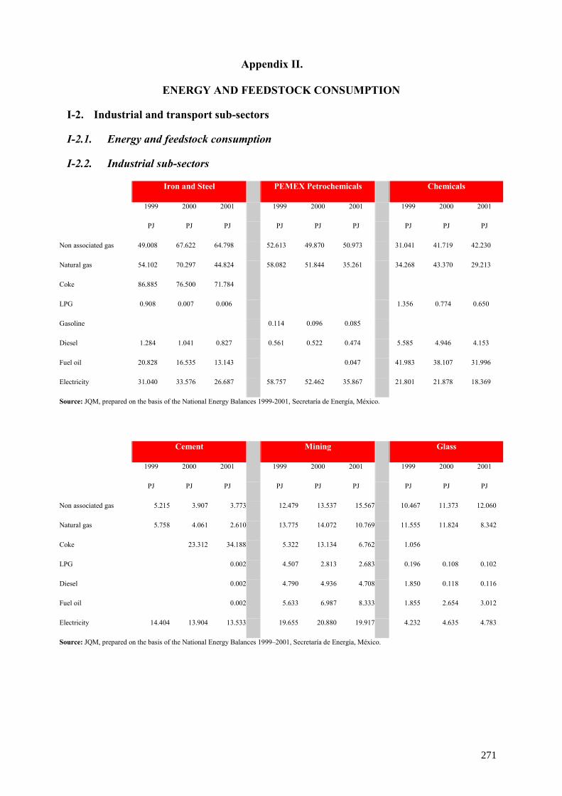
Appendix II.

ENERGY AND FEEDSTOCK CONSUMPTION

I-2. Industrial and transport sub-sectors

I-2.1. Energy and feedstock consumption

I-2.2. Industrial sub-sectors

Iron and Steel PEMEX Petrochemicals Chemicals

1999 2000 2001 1999 2000 2001 1999 2000 2001

PJ PJ PJ PJ PJ PJ PJ PJ PJ

Non associated gas 49.008 67.622 64.798 52.613 49.870 50.973 31.041 41.719 42.230

Natural gas 54.102 70.297 44.824 58.082 51.844 35.261 34.268 43.370 29.213

Coke 86.885 76.500 71.784

LPG 0.908 0.007 0.006 1.356 0.774 0.650

Gasoline 0.114 0.096 0.085

Diesel 1.284 1.041 0.827 0.561 0.522 0.474 5.585 4.946 4.153

Fuel oil 20.828 16.535 13.143 0.047 41.983 38.107 31.996

Electricity 31.040 33.576 26.687 58.757 52.462 35.867 21.801 21.878 18.369

Source: JQM, prepared on the basis of the National Energy Balances 1999-2001, Secretaría de Energía, México.

Cement Mining Glass

1999 2000 2001 1999 2000 2001 1999 2000 2001



Natural gas 5.758 4.061 2.610 13.775 14.072 10.769 11.555 11.824 8.342

Coke 23.312 34.188 5.322 13.134 6.762 1.056

LPG 0.002 4.507 2.813 2.683 0.196 0.108 0.102

Diesel 0.002 4.790 4.936 4.708 1.850 0.118 0.116

Fuel oil 0.002 5.633 6.987 8.333 1.855 2.654 3.012

Electricity 14.404 13.904 13.533 19.655 20.880 19.917 4.232 4.635 4.783

Source: JQM, prepared on the basis of the National Energy Balances 1999–2001, Secretaría de Energía, México.

271

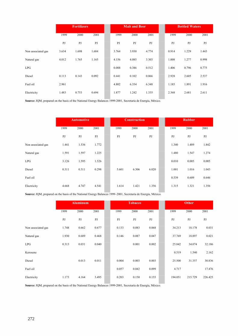
Fertilizers Malt and Beer Bottled Waters

1999 2000 2001 1999 2000 2001 1999 2000 2001



Natural gas 4.012 1.765 1.165 4.156 4.085 3.303 1.008 1.277 0.998

LPG 0.088 0.386 0.512 1.406 0.796 0.775

Diesel 0.113 0.143 0.092 0.441 0.102 0.066 2.928 2.605 2.537

Fuel oil 2.961 4.802 6.354 6.348 1.185 1.891 1.916

Electricity 1.483 0.753 0.694 1.877 1.242 1.335 2.368 2.681 2.611


Automotive Construction Rubber

1999 2000 2001 1999 2000 2001 1999 2000 2001


Non associated gas 1.441 1.536 1.772 1.340 1.489 1.842

Natural gas 1.591 1.597 1.225 1.480 1.547 1.274

LPG 3.126 1.595 1.526 0.010 0.005 0.005

Diesel 0.311 0.311 0.298 5.601 6.306 6.020 1.001 1.016 1.043

Fuel oil 0.539 0.609 0.646

Electricity 4.668 4.747 4.541 1.614 1.421 1.356 1.315 1.321 1.356


Aluminum Tobacco Other

1999 2000 2001 1999 2000 2001 1999 2000 2001



Natural gas 1.930 0.689 0.468 0.146 0.087 0.047 37.769 18.897 0.021

LPG 0.313 0.031 0.040 0.001 0.002 25.842 34.074 32.186

Kerosene 0.519 1.540 2.162

Diesel 0.013 0.011 0.004 0.003 0.003 25.500 31.357 30.836

Fuel oil 0.057 0.042 0.099 4.717 17.476

Electricity 1.173 4.164 3.495 0.203 0.150 0.155 194.051 215.729 226.425


272

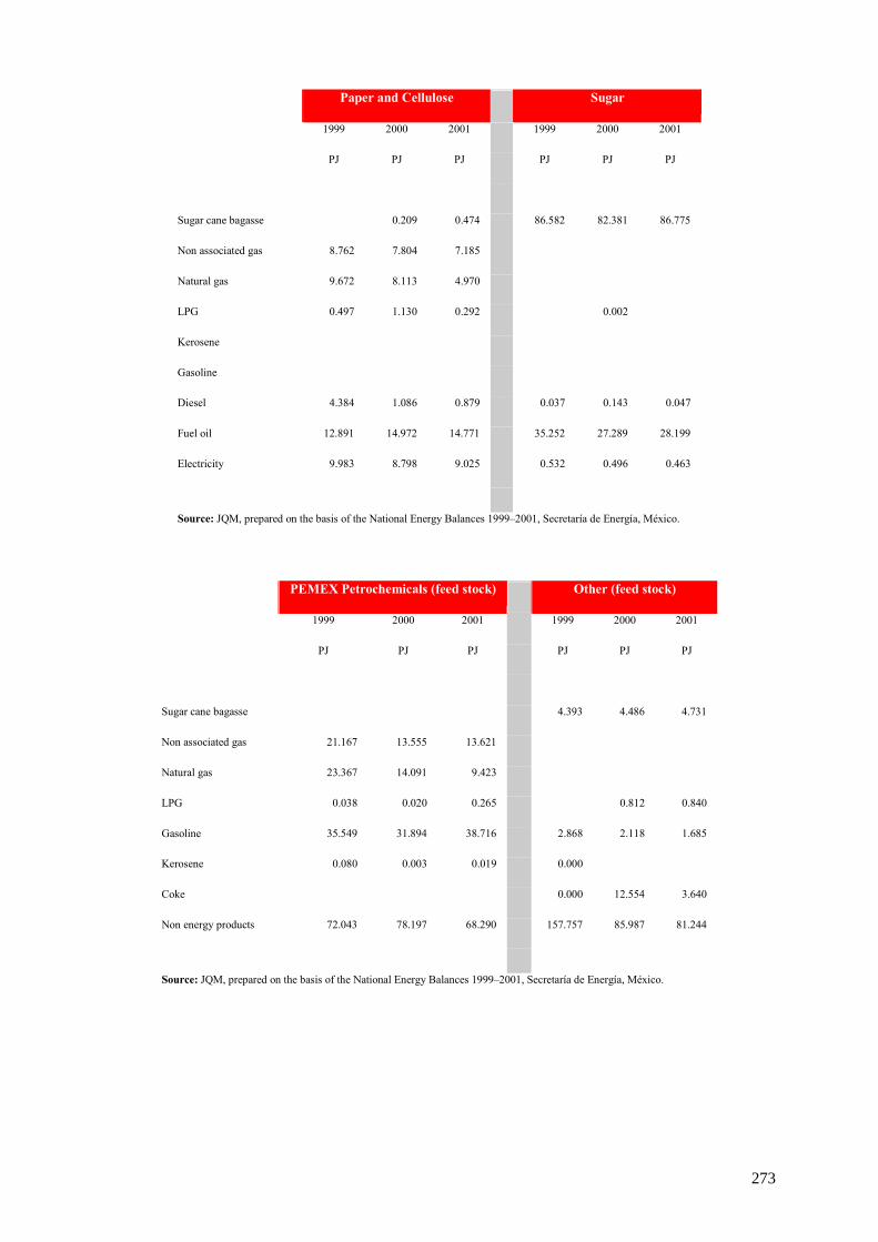
Paper and Cellulose Sugar

1999 2000 2001 1999 2000 2001

PJ PJ PJ PJ PJ PJ

Sugar cane bagasse 0.209 0.474 86.582 82.381 86.775

Non associated gas 8.762 7.804 7.185

Natural gas 9.672 8.113 4.970

LPG 0.497 1.130 0.292 0.002

Kerosene

Gasoline

Diesel 4.384 1.086 0.879 0.037 0.143 0.047

Fuel oil 12.891 14.972 14.771 35.252 27.289 28.199

Electricity 9.983 8.798 9.025 0.532 0.496 0.463


PEMEX Petrochemicals (feed stock) Other (feed stock)

1999 2000 2001 1999 2000 2001

PJ PJ PJ PJ PJ PJ

Sugar cane bagasse 4.393 4.486 4.731


Natural gas 23.367 14.091 9.423

LPG 0.038 0.020 0.265 0.812 0.840

Gasoline 35.549 31.894 38.716 2.868 2.118 1.685

Kerosene 0.080 0.003 0.019 0.000

Coke 0.000 12.554 3.640

Non energy products 72.043 78.197 68.290 157.757 85.987 81.244


273

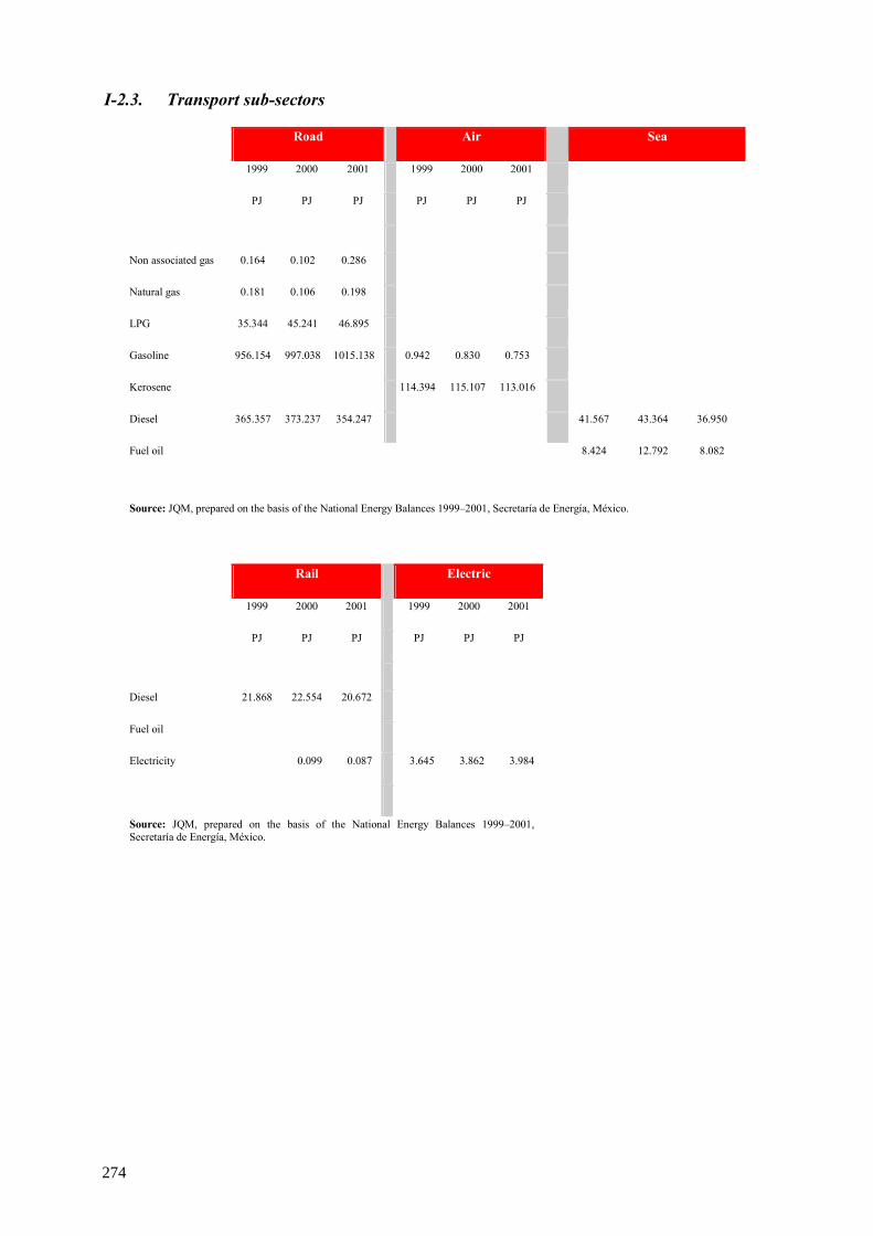
I-2.3. Transport sub-sectors

Road Air Sea

1999 2000 2001 1999 2000 2001

PJ PJ PJ PJ PJ PJ


Natural gas 0.181 0.106 0.198

LPG 35.344 45.241 46.895

Gasoline 956.154 997.038 1015.138 0.942 0.830 0.753

Kerosene 114.394 115.107 113.016

Diesel 365.357 373.237 354.247 41.567 43.364 36.950

Fuel oil 8.424 12.792 8.082


Rail Electric

1999 2000 2001 1999 2000 2001

PJ PJ PJ PJ PJ PJ

Diesel 21.868 22.554 20.672

Fuel oil

Electricity 0.099 0.087 3.645 3.862 3.984


274

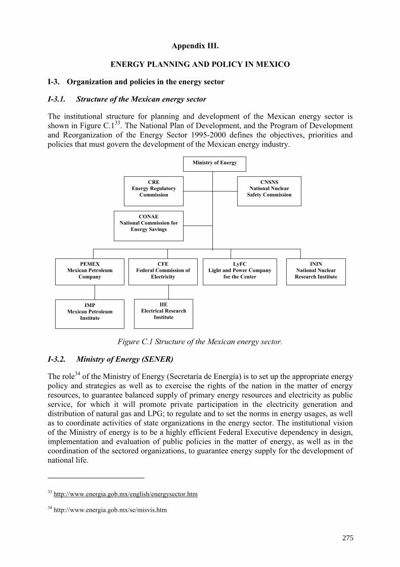
Appendix III.

ENERGY PLANNING AND POLICY IN MEXICO

I-3. Organization and policies in the energy sector

I-3.1. Structure of the Mexican energy sector

The institutional structure for planning and development of the Mexican energy sector is shown in Figure C.133. The National Plan of Development, and the Program of Development and Reorganization of the Energy Sector 1995-2000 defines the objectives, priorities and policies that must govern the development of the Mexican energy industry.

Ministry of Energy

CRE Energy Regulatory

Commission

CNSNS National Nuclear

Safety Commission

CONAE National Commission for

Energy Savings

PEMEX Mexican Petroleum

Company

CFE Federal Commission of

Electricity

LyFC Light and Power Company

for the Center

ININ National Nuclear

Research Institute

IMP Mexican Petroleum

Institute

IIE Electrical Research

Institute

Figure C.1 Structure of the Mexican energy sector.

I-3.2. Ministry of Energy (SENER)

The role34 of the Ministry of Energy (Secretaría de Energía) is to set up the appropriate energy policy and strategies as well as to exercise the rights of the nation in the matter of energy resources, to guarantee balanced supply of primary energy resources and electricity as public service, for which it will promote private participation in the electricity generation and distribution of natural gas and LPG; to regulate and to set the norms in energy usages, as well as to coordinate activities of state organizations in the energy sector. The institutional vision of the Ministry of energy is to be a highly efficient Federal Executive dependency in design, implementation and evaluation of public policies in the matter of energy, as well as in the coordination of the sectored organizations, to guarantee energy supply for the development of national life.

33 http://www.energia.gob.mx/english/energysector.htm

34 http://www.energia.gob.mx/se/misvis.htm

275

In order to obtain it, it must train qualified people, being able to fulfill objectives and goals in an effective and efficient way and with an ample sense of pride to be part of this institution and of the energy sector. Also, the Ministry of Energy must have a flexible and modern organic and functional structure that allows fast adaptation to changes of the national and international surroundings; vanguard infrastructure in computers and telecommunications to support the execution of its attributions and functions; and a transparent handling of the assigned budgetary resources for its operation.

The CRE (Comisión Reguladora de Energía) contributes to safeguard the benefit of public services, fortifies a fair competition, protects user’s shares, propitiates a suitable national cover and takes care of the reliability, stability and security in the supply and services35. The CRE has proposed to promote efficient development of the gas and electrical energy sectors in benefit of the users. In order to carry out this objective, the CRE regulates the natural and legal monopolies in the electrical and natural gas industries in Mexico. The regulating activity has to be conducted in transparent, impartial, and uniform way, based in clear and stable norms. The CRE has developed five basic principles of operation for its regulating activity:

Clarity: the Commission establishes simple and precise rules for the regulated activities;

Stability: the rules are in agreement with a long term vision of the industry to promote the required investments;

Transparency: commissioners, who deliberate in collegian way, take the decisions and their resolutions are registered in a public registry;

Fairness: the law application does not distinguish between public and private entities, the dispositions are of general application and consistent and predictable criteria are applied; and,

Autonomy: the CRE decisions are taken in accordance with objectives and long term vision established in applicable legal dispositions, independently of political conditions.

In Agreement with the National Plan of Development, the regulating activity of the CRE does not have to obstruct or to restrict the productive activity of the individuals, but to promote it. Through an equitable, transparent and efficient frame of regulation, it will be managed to stimulate the competitive capacity of the companies, to encourage the productive investment and to propitiate the creation of more and better jobs in both industry and services

I-3.3. National Commission for Energy Savings (CONAE)

The institutional mission of the CONAE (Comisión Nacional para el Ahorro de Energía) is design, promote and foment guidelines and actions in matter of saving and efficient use of energy and exploitation of renewable energies in the country; to offer technical assistance in this matter to public, private and social sectors; as well as to concert implantation of energy efficiency norms36.

35 http://www.cre.gob.mx/cre/mision.html 36 http://www.conae.gob.mx/quees/mision.html

276

I-3.4. National Commission of Nuclear Security and Safeguards (CNSNS)

The mission of the CNSNS (Comisión Nacional de Seguridad Nuclear y Salvaguardias) is to assure that activities, where nuclear fuels, radioactive and ionizing radiation sources are involved, are realized with maximum security, considering current technological developments37.

I-3.5. Mexican Petroleum Company (PEMEX)

The institutional mission of PEMEX (Petróleos Mexicanos) is to administer in a rational way the hydrocarbons, which are property of the nation, and its own assets in a safe and sustainable way, as well as efficiently supply to the country necessities of petroliferous products, natural gas and basic petrochemical products38. PEMEX is the greatest company of Mexico and one of the ten largest of the world in terms of assets and income. Based in the level of reserves and its extraction capacity and refinement, PEMEX is among the most important oil companies worldwide39. The PEMEX activities include exploration and operation of hydrocarbons, as well as production, storage, distribution and commercialization of petroliferous and petrochemical products. By virtue of which in accordance with the Mexican legislation these activities correspond in exclusive right to the State, PEMEX is a decentralized public organization.

I-3.6. Federal Commission of Electricity (CFE)

CFE (Comisión Federal de Electricidad)40,41 is in charge of assuring the supply of electrical energy in the country, in suitable conditions of amount, quality and price, providing careful attention to the users of the service, as well as protecting the environment, promoting the social development and respect the values of the population where the electrification works are located.

I-3.7. Light and Power Company for the Center (LyFC)

According to the guidelines that are indicated in the Development Plan 1995-2000 and its correlative sector program, the mission of LyFC (Compañía de Luz y Fuerza del Centro) is to provide, in its area of competition, public service of electrical energy as strategic activity that helps economic and social development42,43.

I-3.8. National Nuclear Research Institute (ININ)

The mission of the ININ (Instituto Nacional de Investigaciones Nucleares) is to contribute as a National Laboratory to the research and development of nuclear sciences and its applications, making research of excellence and providing quality services, besides to contribute to the formation of high-level researchers44,45.

37 http://www.cnsns.gob.mx/ 38 Secretaría de Energía, Manual de organización general de las entidades paraestatales 2000: sector energía, p. 142 39 http://www.pemex.com/conozca.html 40 http://www.cfe.gob.mx/git/infomis.html 41 Secretaría de Energía, Manual de organización general de las entidades paraestatales 2000: sector energía p. 35 42 http://www.lfc.gob.mx/mision.htm 43 Secretaría de Energía, Manual de organización general de las entidades paraestatales 2000: sector energía, p. 122. 44 http://www.inin.mx/inin/Dirgral/indiceg.html 45 Secretaría de Energía, Manual de organización general de las entidades paraestatales 2000: sector energía, p. 110

277

I-3.9. Mexican Petroleum Institute (IMP)

The mission of the IMP (Instituto Mexicano del Petróleo) is generate, develop, assimilate and apply scientific and technological knowledge, to promote the development of specialized human resources to support the national oil industry and to contribute to the development maintained and sustainable of the country46,47.

The IMP vision is to be an institution dedicated fundamentally to research and technological development, centered in the generation of knowledge and abilities critics for the oil industry, that transforms knowledge into industrial realities, that offers and commercializes services and products of quality and with high technological content; to be an institution of recognized national and international prestige, organized to respond with agility to the change and able to maintain its financial self-sufficiency.

I-3.10. Electrical Research Institute (IIE)

The mission of the IIE (Instituto de Investigaciones Eléctricas) is to promote and support innovation through value-adding applied research and development to increase the competitiveness of Mexico’s electric industry. The institutional vision of the IIE is to be a leading institute formed by prestigious scientific and technical groups, whose work provides benefits to the national electric industry and to be a source of income for the sustainment of technological endeavors48,49.

I-4. Electric Energy Planning Procedures

In order to determine capacity and location of the new generating power stations, as well as the optimal expansion of the transmission network, is necessary to consider power and energy that are required in each one of the different consumption centers of the country. The starting point is a regional study of the sales of electrical energy, which analyzes the evolution of the sales in each geographic zone and area of the national electrical system. The regional projections are based on complemented statistical studies of tendency with estimations based on requests of big consumers. The studies results of the regional sales are adjusted to tie with the forecasting of regional sales, defined previously with econometric models50.

I-4.1. Expansion of the National Electrical System

The expansion of the national electrical system is based on long term planning for the following reasons51:

• It takes several years of anticipation to make investment decisions of an infrastructure of electrical generation and transmission. It is because the projects have long periods of maturation. From the date in which the construction of a new power station of generation begins to its entrance in commercial operation, approximately four years on average pass. In the case of transmission projects,

46 http://www.imp.mx/mision.htm 47 Secretaría de Energía, Manual de organización general de las entidades paraestatales 2000: sector energía, p. 92 48 Instituto de Investigaciones Eléctricas, Annual Report 1999. 49 http://www.iie.org.mx 50 Secretaria de Energía, Prospectiva del sector eléctrico 2000-2009, p. 78 51 Secretaria de Energía, Prospectiva del sector eléctrico 2000-2009, p. 87

278

about three years are needed. In addition, it is necessary to consider the required time for the formulation, evaluation and authorization of the projects.

• Decisions related to the expansion of the electrical system have economic repercussions in the long term, since lifetime of facilities is of the order of 30 years.

For the planning of the electrical system up-to-date information of the feasible projects of generation and transmission is required to be incorporated in the expansion program. This information comes from the studies of identification and evaluation of projects and technologies, which CFE and LyFC elaborate, as well as of other specialized sources. With such information a feasible project catalogue is done and a document denominated “Costs and Parameters of Reference for the formulation of projects in the electrical sector52” that contains technical parameters and considered costs of typical projects of diverse technologies of generation and transmission.

The program of expansion of the national electrical system is determined by means of a systematic analysis of diverse configurations of feasible projects, that are evaluated technically and economically and in the frame of the electrical system allows to select the projects which minimize the sum of the updated costs of investment, operation and deficit of supply, in the period of planning (optimal program of expansion). For this process models of optimization and simulation are used.

I-4.2. Margin of reserve

The adopted minimum values for the planning of the interconnected system are the following ones53:

• Margin of reserve = 27%

• Margin of operative reserve = 6%

These levels of reserve are considered suitable when there are no restrictions in the transmission network.

For the Baja California area a minimum value is adopted of reserve capacity, after discounting the unavailable capacity by maintenance, whichever is larger:

(a) The capacity of the largest unit, or

(b) 15% of the maximum demand.

For the Baja California Sur area, the total capacity of the two largest units is adopted as the minimum value of reserve capacity.

I-4.3. Analytical tools used in the planning of the energy sector

Descriptions of the analytical tools that are used by the CFE, PEMEX, SENER and Academic Institutions for energy planning at the National and Sectoral level are reported in several

52 Costos y parámetros de referencia para la formulación de proyectos en el sector eléctrico (COPAR) 53 Secretaria de Energía, Documento de Prospectiva del Sector Eléctrico) 2000-2009, p. 90

279

publications by CFE, PEMEX, Academic Institutions, Symposia and Congresses54. The reader is referred to such publications for a detailed knowledge and analysis of the analytical tools, their origin and purpose, status of development and scope of application.

I-5. Recent energy policy and strategies

I-5.1. Current energy policy

The recent policy focuses mainly on the following objectives55:

• Increase the quality of life of the Mexican people;

• Promote a rational use of resources in the context of sustainable development and intergenerational equity;

• Promote investment in productive and feasible projects for Mexico;

• Generate an elastic supply of hydrocarbons;

• Increase productivity in the sector;

• Achieve a competitive pricing policy.

I-5.2. Use of renewable resources

The Federal Government Energy Policy has stimulated the use of renewable resources for the generation of electricity, such as hydroelectric, geothermal, wind, and other energies56,57. The CFE has identified a potential 52 900 MW58 in a diverse hydroelectric exploitation sites throughout the country, of which about 10 000 MW have been harnessed by the CFE and private investors under the modality of self-supply, for industrial as well as municipal use could develop 42 900 MW. This potential store is integrated by projects under divers level of research, which go from identification of hydroelectric potential to develop studies carried out by the CFE in the last few years. The size of these projects is between 20 MW and 700 MW.

With respect to geothermal exploitation sites, there are several such as Los Azufres, in Michoacan, and others, where underground vapor could be used to develop projects for generation of electricity.

The Tehuantepec Isthmus area is known worldwide for its great aeolian potential, estimated in 2 000 MW. At the beginning of 1998, the CRE, awarded self-supply permit of 30 MW for a wind project at La Venta, Oaxaca, as well as an additional permit for another self-supply project of 60 MW in Baja California, which is also an area of very high wind potential.

54 Modelos Matemáticos para la Planeación Energética, Quintanilla, J. (Ed), Programa Universitario de Energía, Dirección

General de Servicios de Cómputo Académico, UNAM, México,1983. 55 http://www.energia.gob.mx/english/energysector.htm 56 http://www.energia.gob.mx/english/oielectricoi.html 57 More information can be found in the Electrical Sector Prospective Brief 2000-2009, pages 135-139 58 CFE, Catalog of hydroelectric projects (Catálogo de proyectos hidroeléctricos), June 2000

280

Appendix IV.

ELECTRICITY PRODUCTION CHAINS FOR OIL AND GAS

I-6. Oil and gas production, processing, transportation and their environmental impacts: A general view

I-6.1. Oil and natural gas chains

Fuel oil and diesel, two by-products of the petroleum industry, are used as boiler fuels in thermal plants for electricity production, but they have other energy applications also. Natural gas, with a carbon to energy ratio that is less than half that of coal, and about two-thirds that of oil, may receive strong attention as a fuel for generating electricity, as is the case at present, when there is need to minimize CO2 emissions. So far as the greenhouse effect is concerned, this advantage may be put in jeopardy due to releases of methane during the gas extraction, transportation and handling. Therefore, it is necessary to consider the full energy chain and consider that there are options for the reduction of such methane losses. The impacts from the oil and gas chains for electricity generation are associated with the overall activities for the oil and gas exploration, production, processing and transportation.

I-6.2. Oil and gas production

Exploration and production of oil and natural gas, onshore and offshore, have a number of environmental impacts. Fires, explosions and accidental spills are the most common accidents. Accidents and equipment failures can cause harm to workers and environment. These activities require a substantial support in terms of technologies and specialized personnel and are provided from places, as near as possible, to the production field. In the case of offshore production fields these support installations are located on the nearest coastal location putting pressure on the local infrastructure (housing, community services) and social conditions. The sitting of the necessary facilities, such as pipelines, pipelines terminals and platform construction sites, leads to land management problems, since it competes with other possible uses of the coastal zone. For onshore production fields the situation is similar to the offshore ones, however it has the advantage to be inland. Although accidental spills from offshore and on shore operations are, normally, of relative small volumes, some large spills have occurred in the past. Even with careful treatment of effluent discharges and stringent controls to minimize accidental oil spillage, both onshore and offshore oil and gas production result in some discharge to the surrounding environment. Tidal marshes, coastal wetlands, rivers, swamps and sheltered bays are sensitive ecosystems; even low levels of hydrocarbon pollution can originate serious ecological impacts.

Presently, oil and natural gas operations have the tendency to work at higher depths (onshore and offshore) and under harsher environments than in the past. There may be a possibility that higher environmental risks may occur under these conditions, conditions that may be different from those experienced in the past.

Crude oil frequently is associated with large amounts of emulsified brine. After separation, the brine usually is disposed of by re-injection into the earth. However, some brine may be discharged to marine or terrestrial water bodies, which can have serious effects on aquatic ecosystems. During natural gas extraction, there are some leaks. Since natural gas is mainly methane, a strong greenhouse gas, there are some concerns that these leakages can add to the possible risks of global warming.

281

Besides the already mentioned sources of pollution of air and water, for the analysis we have to take into account other sources of contamination under normal conditions of operation. These additional sources of emissions are related to the energy uses for extraction, reinjection and other services that are needed for the separation of oil and natural gas and its shipment into the storage facilities. Compressors, electricity generators and other equipment require a source of energy for its operations. Electricity, diesel and natural gas can provide the required energy for this equipment. Normally, offshore facilities employee diesel generators to produce the required electricity and mechanical work for their operations.

Once crude oil and natural gas have been separated, at the separation batteries, they are sent, through pipelines, to the storage facilities for shipment into the crude oil processing centers (refineries), to the processing gas plants and preparation for export to other countries.

I-6.3. Oil transportation

Usually, oil has to be transported over long distances, because the area of oil production does not coincide with either the area of processing or demand. Marine transportation and pipelines are the two modes of crude oil transportation.

Marine oil tankers are the most important means of international oil transportation. As in many oil activities, oil transportation has some risks to suffer accidents and, therefore, can have serious effects on the environment and marine life. Wind and ocean currents can move oil for long distances in a relatively short time, and the consequences of a major spillage can be spread over a large area. Oil discharge and cleaning of oil tankers after unloading represent another danger to oceans and coastal ecosystems. Some tankers are filled with water as ballast after the oil is unloaded, and the ballast water becomes contaminated with oil residues. The discharge of water contaminated with oil, before taking a new oil cargo, adds to oil pollution of the oceans. The oil industry has introduced a variety of methods, such as using crude oil instead of water for tanker cleaning, to mitigate such operational pollution.

Oil terminals often are constructed within or near ecologically sensitive coastal areas, such as estuaries. There always exist the risk of oil spillage during the transfer of oil from the tanker or from the marine oil fields to the shore facility. Even in the absence of large scale oil spills the cumulative effect of many small spills and leaks remains in the area. Because oil floats on the sea surface, spilled oil tends to become deposited in the intertidal zone near or on the shoreline, causing many undesirable consequences. Suitable surface treatment agents can be used for the protection of shorelines from the spills. These are emulsifying agents that can be used to disperse the oil in the water; nevertheless ocean waters become polluted.

Compared to marine oil transport, pipelines in general present lesser environmental problems. For offshore facilities they are generally laid on the ocean floor. Burial of pipe lines which lie in less than 100 meters of water is usually required. Doing so minimizes the potential for damage from natural forces and from marine equipment. Onshore, pipelines are laid in trenches. For large distances, remote control valves at varying distances along the pipelines are installed to minimize the possibility of large oil spills, in case of damage. Pipelines which are not buried in the ground can cause disturbances to wildlife. Natural forces, such as earthquakes and corrosion, also have to be considered.

Natural gas consists of methane and other hydrocarbon compounds, and usually is transported in gaseous form through pipelines. The primary risks with gas pipelines are associated with fires and explosions, in particular from pipelines passing through or near heavily populated

282

areas. In addition, pipeline leakage of methane, a strong greenhouse gas; contribute to the potential risks of climate change and global warming.

For ocean transport, natural gas is cooled to its liquid state (liquefied natural gas, LNG) for transport by special LNG tankers. The main environmental effects associated with natural gas liquefaction plants are the discharge of heat to the atmosphere or to fresh or marine waters, depending on the type of cooling system used, and the occasional emission or flaring of some components extracted during gas liquefaction. There is also a possibility of destructive evaporation of LNG if it comes in contact with water.

I-6.4. Oil processing (refining)

Refineries are large industrial installations with air and water emissions, large water requirements for processing and cooling, and risks of explosions and fires. The principal types of airborne emissions are volatile hydrocarbons, sulfur oxides, nitrogen oxides and particulate. Some amounts of carbon monoxide, volatile organic compounds and ammonia are emitted also. In addition, there are important amounts of CO2 and unburned hydrocarbons due to the energy consumption (oil products, natural gas and electricity) in the different processes. Liquid effluents contain chlorides, grease, ammonia nitrate, phosphate, suspended solids, dissolved solids and trace metals (V, Cr, Pb, Zn, Cu, etc.).

Refineries require large amounts of water, mainly for cooling and various process operations. Each process operation has different water usage and wastewater characteristics associated with it. In addition to process wastewater, ballast water in tanks, storm water runoff and sanitary wastes contribute to the total wastewater load that must be treated before discharge to the environment.

The most significant pollutants present in this waste load are oil and grease, phenols, ammonia, suspended and dissolved solids, sulfites and chromium. Treatment techniques consist mainly of primary separation of oil and solids and neutralization, followed by biological treatment using activated sludge systems, aerated lagoons or oxidation ponds. Unpleasant odor is another potential nuisance in and around refineries. Hydrogen sulfide (H2S) and mercaptans are the principal malodorous compounds. Even small leakage of these compounds from a refinery can cause unpleasant smells in the surrounding area.

Accidental spills of stored crude oil or refined products can cause severe local environmental impacts, requiring extensive restoration efforts.

The petroleum refining industry converts crude oil into more than 2 500 products, including liquefied petroleum gas, gasoline, kerosene, aviation fuel, diesel fuel, fuel oils, lubricating oils, and feedstock for the petrochemical industry. Petroleum refinery activities start with the receipt of crude oil for storage at the refinery, include all petroleum handling and refining operations, and terminate with storage preparatory to shipping the refined products from the refinery.

The petroleum refining industry employs a wide variety of processes. The composition of crude oil feedstock and the chosen slate of petroleum products largely determine a refinery's processing flow scheme. The refinery flow scheme presented in Figure D.1 shows the general processing arrangement for major refinery processes. The arrangement of these processes will vary among refineries, and not all the refineries will employ all of these processes. Petroleum refining processes having direct emission sources are presented in bold-line boxes on the Figure.

283

Generally speaking, one can consider five categories of refinery processes and associated operations. These categories are: a) separation processes (atmospheric distillation, vacuum distillation and light ends recovery (gas processing)); b) petroleum conversion processes (cracking (thermal and catalytic), reforming, alkylation, polymerization, isomerization, coking and visbreaking); c) petroleum treating processes (hydrotreating, hydrodesulfurization, chemical sweetening, acid gas removal and deasphalting); d) feedstock and product handling (storage, blending, loading and unloading); and e) auxiliary facilities (boilers, wastewater treatment, hydrogen production, sulfur recovery plant, cooling towers, blow down system and compressor engines).

According to Figure D.1, several of these processes have direct and significant contributions to the air pollution. Bold-line boxes on Figure D.1 identify those processes. The major sources of atmospheric emissions from the vacuum distillation column are associated with the steam ejectors or vacuum pumps. A second source of atmospheric emissions from vacuum distillation columns is combustion products from the process heater. Fugitive hydrocarbon emissions from leaking seals and fittings are also associated with the vacuum distillation unit.

Catalytic cracking, using heat, pressure and catalysts, converts heavy oils into lighter products with product distributions favoring the more valuable gasoline and distillate blending components. All the catalytic cracking processes in use today can be classified as either fluidized bed or moving bed units. Air emissions from catalytic cracking processes are combustion products from process heaters and flue gas from catalyst regeneration. Emissions from process heaters consist of all pollutants. The quantity of these emissions is a function of the type of fuel burned, the nature of the contaminants in the fuel, and the heat duty of the furnace. Among those contaminants are sulfur oxide, carbon monoxide, nitrogen oxides and particulate. Emissions from the catalyst regenerator include hydrocarbons, oxides of sulfur, ammonia, aldehydes, oxides of nitrogen, cyanides, carbon monoxide and particulate.

Thermal cracking processes include visbreaking and coking. Air emissions from thermal cracking processes include coke dust from decoking operations, combustion gases from the visbreaking and coking process heaters, and fugitive emissions.

Particulate emissions from delayed coking operations are potentially significant. These emissions are associated with removing the coke from the coke drum and subsequent handling and storage operations. Hydrocarbon emissions are also associated with cooling and venting the coke drum prior to coke removal.

The utility plant supplies the steam necessary for the refinery. Although the steam can be used to produce electricity (as is the case in most of the Mexico's refinery facilities), it is primarily used for heating and separating hydrocarbon streams. When used for heating, the steam usually heats the petroleum indirectly in heat exchangers and returns to the boiler. In direct contact operations, the steam can serve as a stripping medium or a process fluid. Steam may also be used in vacuum ejectors to produce a vacuum. Emissions from boilers were commented in a previous paragraph.

Sulfur recovery plants are used in petroleum refineries to convert hydrogen sulfide (H2S) separated from refinery gas streams into the more disposable by-product, elemental sulfur. Emissions from sulfur recovery unit contain sulfur dioxide, carbon monoxide, volatile organic compounds and other reduced sulfur compounds.

284

Most refining units and equipment subject to planned or unplanned hydrocarbon discharges are manifold into a collection unit, called the blow down system. By using a series of flash drums and condensers arranged in decreasing pressure, the blow down is separated into vapor and liquid cuts. The separated liquid is recycled into the refinery. The gaseous cuts can either be smokeless flared or recycled. Therefore, the combustion of the noncondensables in a flare is a source of emissions. Complete combustion or smokeless burning can be carried out by the addition of steam in the combustion zone of the flare and reduce emissions of nitrogen oxides due to the lowering of the flame temperature.

Refining units operating al high pressure include hydrodesulfurization, isomerization, reforming and hydrocracking. These units require compressor engines (reciprocating and gas turbine) fired with natural gas or some other fossil fuel. Internal combustion engines are less reliable and harder to maintain than steam engines or electric motors. The major source of emissions from compressor engines is combustion products in the exhaust gas. These emissions include carbon monoxide, hydrocarbons, nitrogen oxides, aldehydes and ammonia. Sulfur oxides may also be present, depending on the sulfur content of the fossil fuel used.

Sweetening of distillates is accomplished by the conversion of mercaptans to alkyl disulfides in the presence of a catalyst. The extracted distillate is then contacted with air to convert mercaptans to disulfides. After oxidation, the distillate is settled, inhibitors are added, and the distillate is sent to storage. The major emission problem is hydrocarbons from contact between the distillate product and air in the "air blowing" step.

Fugitive emission sources are generally defined as volatile organic compound (VOC) emission sources not associated with a specific process but scattered throughout the refinery. Fugitive VOC emissions are attributable to the evaporation of leaked or spilled petroleum liquids and gases. Valves, flanges, pump and compressor seals, process drains, cooling towers, and oil/water separators are sources of fugitive emissions.

According to the US-EPA59, for these sources, a very high correlation has been found between mass emission rates and the type of stream service in which the sources are employed. Except for compressed gases, streams are classified into one of three stream groups, (1) gas/vapor streams, (2) light liquid/two phase streams, and (3) kerosene and heavier liquid streams. Gasses passing through compressors are classified as either hydrogen or hydrocarbon service. Sources in gas/vapor stream service have higher emission rates then those in heavier stream service. It seems that valves, because of their number and relatively high emission factor, are the major emission source among the source types.

Storage vessels containing organic liquids can be found in the petroleum producing and refining, petrochemical and chemical manufacturing and bulk and transfer operations. Organic liquids in the petroleum industry, usually called petroleum liquids, generally are mixtures of hydrocarbons having dissimilar true vapor pressures (for example, gasoline and crude oil). Clearly, emissions from organic liquids in storage depend upon the tank type and operation activities as well as upon physical conditions of temperature and barometric pressure. Generally speaking, evaporative emissions from storage tanks can be classified as breathing, working and standing storage losses.

59 Assessment of Atmospheric Emissions from Petroleum Refining, U. S. Environmental Protection Agency, Research

Triangle Park, NC, 1980.

285

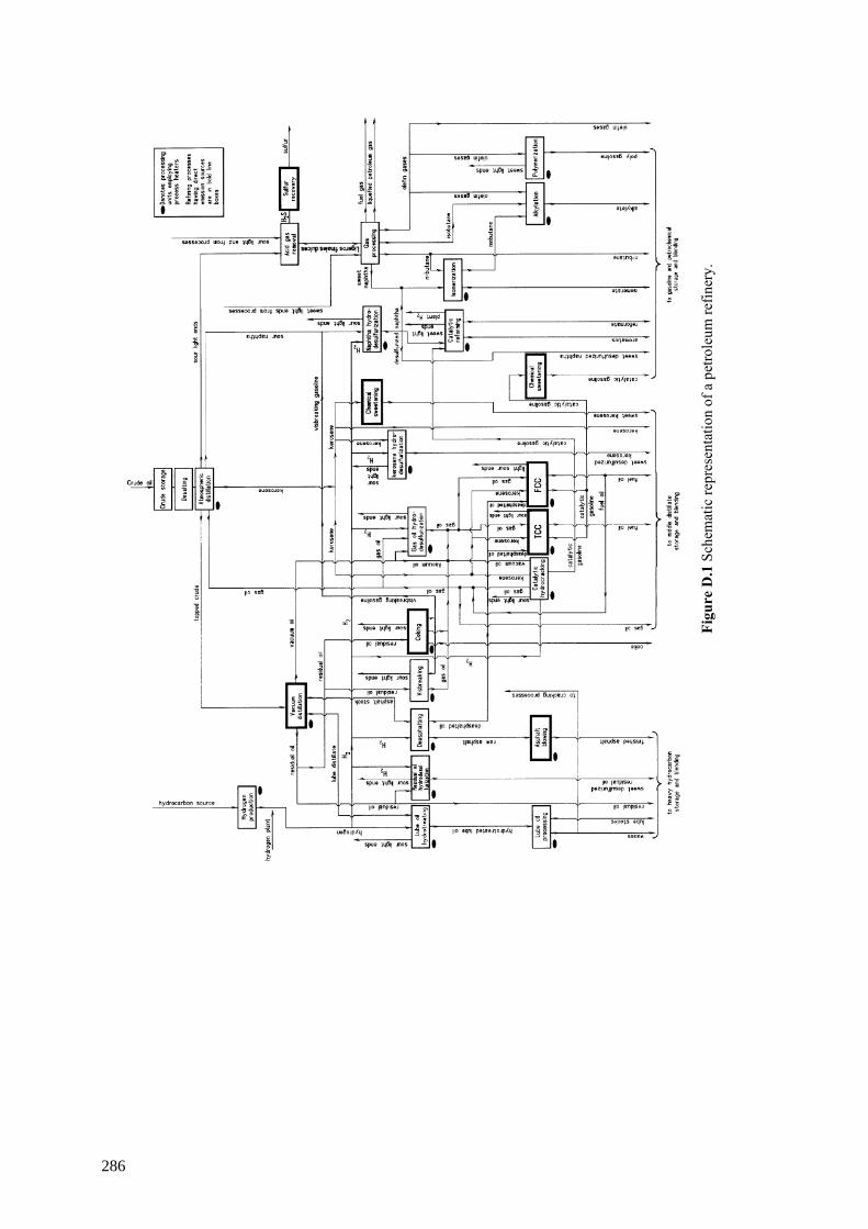
Figu

re D

.1 S

chem

atic

repr

esen

tatio

n of

a p

etro

leum

refin

ery.

286

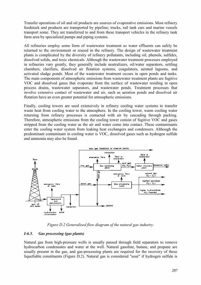
Transfer operations of oil and oil products are sources of evaporative emissions. Most refinery feedstock and products are transported by pipeline; trucks, rail tank cars and marine vessels transport some. They are transferred to and from these transport vehicles in the refinery tank farm area by specialized pumps and piping systems.

All refineries employ some form of wastewater treatment so water effluents can safely be returned to the environment or reused in the refinery. The design of wastewater treatment plants is complicated by the diversity of refinery pollutants, including oil, phenols, sulfides, dissolved solids, and toxic chemicals. Although the wastewater treatment processes employed in refineries vary greatly, they generally include neutralizers, oil/water separators, settling chambers, clarifiers, dissolved air flotation systems, coagulators, aerated lagoons, and activated sludge ponds. Most of the wastewater treatment occurs in open ponds and tanks. The main components of atmospheric emissions from wastewater treatment plants are fugitive VOC and dissolved gases that evaporate from the surface of wastewater residing in open process drains, wastewater separators, and wastewater ponds. Treatment processes that involve extensive contact of wastewater and air, such as aeration ponds and dissolved air flotation have an even greater potential for atmospheric emissions.

Finally, cooling towers are used extensively in refinery cooling water systems to transfer waste heat from cooling water to the atmosphere. In the cooling tower, warm cooling water returning from refinery processes is contacted with air by cascading through packing. Therefore, atmospheric emissions from the cooling tower consist of fugitive VOC and gases stripped from the cooling water as the air and water come into contact. These contaminants enter the cooling water system from leaking heat exchangers and condensers. Although the predominant contaminant in cooling water is VOC, dissolved gases such as hydrogen sulfide and ammonia may also be found.

Figure D.2 Generalized flow diagram of the natural gas industry.

I-6.5. Gas processing (gas plants)

Natural gas from high-pressure wells is usually passed through field separators to remove hydrocarbon condensates and water at the well. Natural gasoline, butane, and propane are usually present in the gas, and gas-processing plants are required for the recovery of these liquefiable constituents (Figure D.2). Natural gas is considered "sour" if hydrogen sulfide is

287

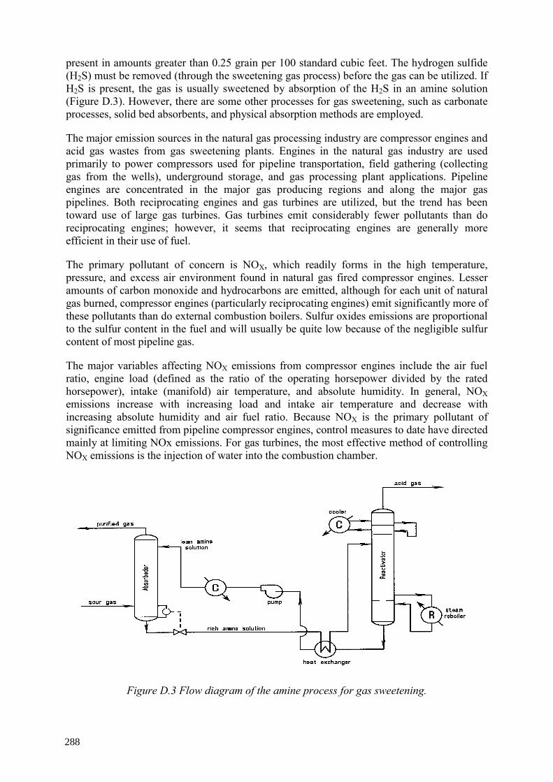
present in amounts greater than 0.25 grain per 100 standard cubic feet. The hydrogen sulfide (H2S) must be removed (through the sweetening gas process) before the gas can be utilized. If H2S is present, the gas is usually sweetened by absorption of the H2S in an amine solution (Figure D.3). However, there are some other processes for gas sweetening, such as carbonate processes, solid bed absorbents, and physical absorption methods are employed.

The major emission sources in the natural gas processing industry are compressor engines and acid gas wastes from gas sweetening plants. Engines in the natural gas industry are used primarily to power compressors used for pipeline transportation, field gathering (collecting gas from the wells), underground storage, and gas processing plant applications. Pipeline engines are concentrated in the major gas producing regions and along the major gas pipelines. Both reciprocating engines and gas turbines are utilized, but the trend has been toward use of large gas turbines. Gas turbines emit considerably fewer pollutants than do reciprocating engines; however, it seems that reciprocating engines are generally more efficient in their use of fuel.

The primary pollutant of concern is NOX, which readily forms in the high temperature, pressure, and excess air environment found in natural gas fired compressor engines. Lesser amounts of carbon monoxide and hydrocarbons are emitted, although for each unit of natural gas burned, compressor engines (particularly reciprocating engines) emit significantly more of these pollutants than do external combustion boilers. Sulfur oxides emissions are proportional to the sulfur content in the fuel and will usually be quite low because of the negligible sulfur content of most pipeline gas.

The major variables affecting NOX emissions from compressor engines include the air fuel ratio, engine load (defined as the ratio of the operating horsepower divided by the rated horsepower), intake (manifold) air temperature, and absolute humidity. In general, NOX emissions increase with increasing load and intake air temperature and decrease with increasing absolute humidity and air fuel ratio. Because NOX is the primary pollutant of significance emitted from pipeline compressor engines, control measures to date have directed mainly at limiting NOx emissions. For gas turbines, the most effective method of controlling NOX emissions is the injection of water into the combustion chamber.

Figure D.3 Flow diagram of the amine process for gas sweetening.

288

Steam injection can provide a second method, however it is necessary to produce the steam. Also, exhaust gas re-circulation can reduce the NOX emissions but they must be cooled before re-injection. Some of these methods are also applicable, in some extension, to reciprocating gas-fired engines. It seems that the most effective NOX control measures for reciprocating gas-fired engines are those that change the air-fuel ratio. Thus, changes in the engine torque, speed, intake air temperature, etc., which in turn increase the air-fuel ratio may all result in lower NOX emissions. Besides NOX emission there are contributions of CO, hydrocarbons, sulfur dioxide and particulate.

The amine type method for sweetening natural gas is shown in Figure D.3. The recovered hydrogen sulfide gas stream may be (1) vented, (2) flared in waste gas flares or modern smokeless flares, (3) incinerated, or (4) utilized in the production of elemental sulfur or other commercial products. If the recovered H2S gas stream is not to be utilized as a feedstock for commercial applications, the gas is usually passed to a tail gas incinerator in which the H2S is oxidized to sulfur dioxide and then passed to the atmosphere via a stack. Emissions will only result from gas sweetening plants if the acid waste gas from the amine process is flared or incinerated. Most often, the acid waste gas is used as a feedstock in nearby sulfur recovery or sulfuric acid plants.

289

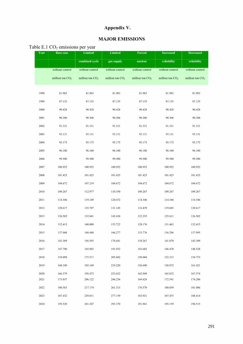
Appendix V.

MAJOR EMISSIONS Table E.1 CO2 emissions per year

Year Base case Limited Limited Forced Increased Decreased

combined cycle gas supply nuclear reliability reliability

without control without control without control without control without control without control

million ton CO2 million ton CO2 million ton CO2 million ton CO2 million ton CO2 million ton CO2

1998 81.983 81.983 81.983 81.983 81.983 81.983

1999 87.135 87.135 87.135 87.135 87.135 87.135

2000 90.428 90.428 90.428 90.428 90.428 90.428

2001 90.306 90.306 90.306 90.306 90.306 90.306

2002 91.331 91.331 91.331 91.331 91.331 91.331

2003 93.131 93.131 93.131 93.131 93.131 93.131

2004 95.175 95.175 95.175 95.175 95.175 95.175

2005 96.180 96.180 96.180 96.180 96.180 96.180

2006 99.500 99.500 99.500 99.500 99.500 99.500

2007 100.952 100.952 100.952 100.952 100.952 100.952

2008 101.425 101.425 101.425 101.425 101.425 101.425

2009 104.672 107.219 104.672 104.672 104.672 104.672

2010 109.267 112.977 110.350 109.267 109.267 109.267

2011 114.346 119.149 120.472 114.346 114.346 114.346

2012 120.617 125.707 131.145 116.439 119.683 120.617

2013 126.502 132.841 142.436 122.255 125.611 126.502

2014 132.415 140.000 153.722 128.176 131.463 132.415

2015 137.048 148.448 166.277 133.776 136.296 137.995

2016 143.389 156.593 178.441 139.267 141.870 143.389

2017 147.790 165.983 191.932 143.685 146.470 148.528

2018 154.098 175.517 205.602 150.060 152.313 154.753

2019 160.109 185.169 219.220 156.690 158.872 161.421

2020 166.379 195.472 233.622 162.949 165.832 167.574

2021 173.037 206.122 246.236 169.624 172.541 174.206

2022 180.563 217.174 261.315 176.570 180.059 181.086

2023 187.432 229.011 277.159 183.921 187.475 188.414

2024 195.520 241.287 293.370 191.961 195.159 196.515

291

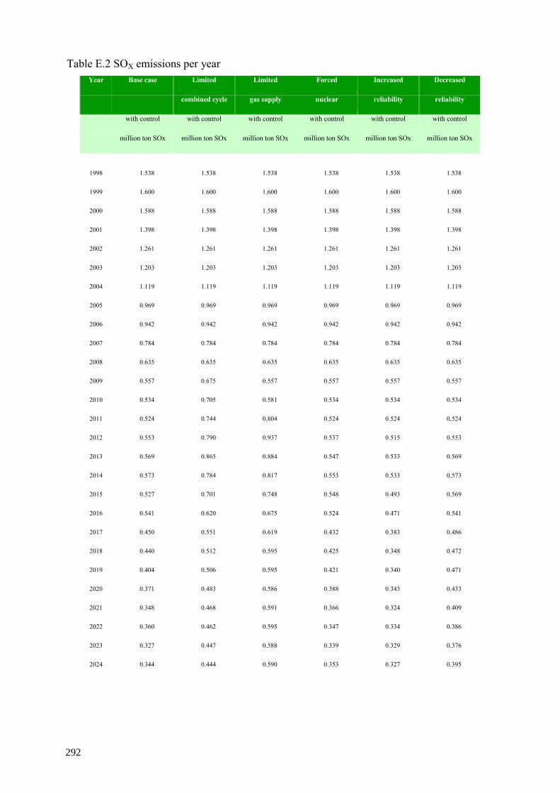
Table E.2 SOX emissions per year Year Base case Limited Limited Forced Increased Decreased


with control with control with control with control with control with control

million ton SOx million ton SOx million ton SOx million ton SOx million ton SOx million ton SOx

1998 1.538 1.538 1.538 1.538 1.538 1.538

1999 1.600 1.600 1.600 1.600 1.600 1.600

2000 1.588 1.588 1.588 1.588 1.588 1.588

2001 1.398 1.398 1.398 1.398 1.398 1.398

2002 1.261 1.261 1.261 1.261 1.261 1.261

2003 1.203 1.203 1.203 1.203 1.203 1.203

2004 1.119 1.119 1.119 1.119 1.119 1.119

2005 0.969 0.969 0.969 0.969 0.969 0.969

2006 0.942 0.942 0.942 0.942 0.942 0.942

2007 0.784 0.784 0.784 0.784 0.784 0.784

2008 0.635 0.635 0.635 0.635 0.635 0.635

2009 0.557 0.675 0.557 0.557 0.557 0.557

2010 0.534 0.705 0.581 0.534 0.534 0.534

2011 0.524 0.744 0.804 0.524 0.524 0.524

2012 0.553 0.790 0.937 0.537 0.515 0.553

2013 0.569 0.865 0.884 0.547 0.533 0.569

2014 0.573 0.784 0.817 0.553 0.533 0.573

2015 0.527 0.701 0.748 0.548 0.493 0.569

2016 0.541 0.620 0.675 0.524 0.471 0.541

2017 0.450 0.551 0.619 0.432 0.383 0.486

2018 0.440 0.512 0.595 0.425 0.348 0.472

2019 0.404 0.506 0.595 0.421 0.340 0.471

2020 0.371 0.483 0.586 0.388 0.343 0.433

2021 0.348 0.468 0.591 0.366 0.324 0.409

2022 0.360 0.462 0.595 0.347 0.334 0.386

2023 0.327 0.447 0.588 0.339 0.329 0.376

2024 0.344 0.444 0.590 0.353 0.327 0.395

292

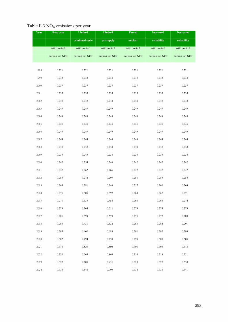
Table E.3 NOX emissions per year Year Base case Limited Limited Forced Increased Decreased



million ton NOx million ton NOx million ton NOx million ton NOx million ton NOx million ton NOx

1998 0.221 0.221 0.221 0.221 0.221 0.221

1999 0.233 0.233 0.233 0.233 0.233 0.233

2000 0.237 0.237 0.237 0.237 0.237 0.237

2001 0.235 0.235 0.235 0.235 0.235 0.235

2002 0.248 0.248 0.248 0.248 0.248 0.248

2003 0.249 0.249 0.249 0.249 0.249 0.249

2004 0.248 0.248 0.248 0.248 0.248 0.248

2005 0.245 0.245 0.245 0.245 0.245 0.245

2006 0.249 0.249 0.249 0.249 0.249 0.249

2007 0.244 0.244 0.244 0.244 0.244 0.244

2008 0.238 0.238 0.238 0.238 0.238 0.238

2009 0.238 0.245 0.238 0.238 0.238 0.238

2010 0.242 0.254 0.246 0.242 0.242 0.242

2011 0.247 0.262 0.266 0.247 0.247 0.247

2012 0.258 0.272 0.297 0.251 0.253 0.258

2013 0.263 0.281 0.346 0.257 0.260 0.263

2014 0.271 0.305 0.397 0.264 0.267 0.271

2015 0.271 0.335 0.454 0.268 0.268 0.274

2016 0.279 0.364 0.511 0.273 0.274 0.279

2017 0.281 0.399 0.573 0.275 0.277 0.283

2018 0.288 0.431 0.632 0.283 0.284 0.291

2019 0.295 0.460 0.688 0.291 0.292 0.299

2020 0.302 0.494 0.750 0.298 0.300 0.305

2021 0.310 0.529 0.800 0.306 0.308 0.313

2022 0.320 0.565 0.863 0.314 0.318 0.321

2023 0.327 0.605 0.931 0.323 0.327 0.330

2024 0.338 0.646 0.999 0.334 0.336 0.341

293

Table E.4 Particle emissions per year Year Base case Limited Limited Forced Increased Decreased



million ton particle million ton particle million ton particle million ton particle million ton particle million ton particle

1998 0.094 0.094 0.094 0.094 0.094 0.094

1999 0.098 0.098 0.098 0.098 0.098 0.098

2000 0.097 0.097 0.097 0.097 0.097 0.097

2001 0.084 0.084 0.084 0.084 0.084 0.084

2002 0.072 0.072 0.072 0.072 0.072 0.072

2003 0.068 0.068 0.068 0.068 0.068 0.068

2004 0.063 0.063 0.063 0.063 0.063 0.063

2005 0.054 0.054 0.054 0.054 0.054 0.054

2006 0.052 0.052 0.052 0.052 0.052 0.052

2007 0.043 0.043 0.043 0.043 0.043 0.043

2008 0.034 0.034 0.034 0.034 0.034 0.034

2009 0.029 0.036 0.029 0.029 0.029 0.029

2010 0.028 0.038 0.030 0.028 0.028 0.028

2011 0.027 0.040 0.044 0.027 0.027 0.027

2012 0.029 0.043 0.052 0.028 0.027 0.029

2013 0.030 0.048 0.051 0.028 0.028 0.030

2014 0.030 0.043 0.048 0.029 0.028 0.030

2015 0.027 0.039 0.046 0.029 0.025 0.030

2016 0.028 0.035 0.043 0.027 0.024 0.028

2017 0.023 0.032 0.041 0.022 0.019 0.025

2018 0.022 0.030 0.041 0.021 0.017 0.024

2019 0.020 0.031 0.043 0.021 0.016 0.024

2020 0.018 0.030 0.044 0.019 0.016 0.022

2021 0.017 0.030 0.045 0.018 0.015 0.020

2022 0.017 0.030 0.047 0.016 0.016 0.019

2023 0.015 0.030 0.048 0.016 0.015 0.018

2024 0.016 0.031 0.050 0.017 0.015 0.019

294

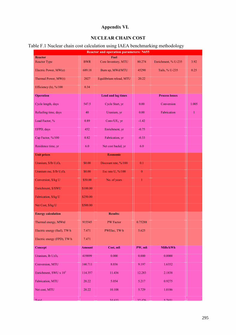
Appendix VI.

NUCLEAR CHAIN COST Table F.1 Nuclear chain cost calculation using IAEA benchmarking methodology

Reactor and operation parameters: N655 Reactor Fuel Reactor Type BWR Core Inventory, MTU 80.274 Enrichment, % U-235 3.92

Electric Power, MW(e) 689.18 Burn up, MWd/MTU 45290 Tails, % U-235 0.25

Thermal Power, MW(t) 2027 Equilibrium reload, MTU 20.22

Efficiency (h), %/100 0.34

Operation Lead and lag times Process losses

Cycle length, days 547.5 Cycle Start, yr 0.00 Conversion 1.005

Refueling time, days 40 Uranium, yr 0.00 Fabrication 1

Load Factor, % 0.89 Conv/UF6, yr -1.42

EFPD, days 452 Enrichment, yr -0.75

Cap Factor, %/100 0.82 Fabrication, yr -0.33

Residence time, yr 6.0 Net cost backd, yr 6.0

Unit prices Economic

Uranium, $/lb U3O8 $0.00 Discount rate, %/100 0.1

Uranium esc, $/lb U3O8 $0.00 Esc rate U, %/100 0

Conversion, $/kg U $50.00 No. of years 1

Enrichment, $/SWU $100.00

Fabrication, $/kg U $250.00

Net Cost, $/kg U $500.00

Energy calculation Results:

Thermal energy, MWtd 915545 PW Factor 0.75288

Electric energy (fuel), TW·h 7.471 PWElec, TW·h 5.625

Electric energy (FPD), TW·h 7.471

Concept Amount Cost, m$ PW, m$ Mills/kWh

Uranium, lb U3O8 419899 0.000 0.000 0.0000

Conversion, MTU 160.711 8.036 9.197 1.6352

Enrichment, SWU x 103 114.357 11.436 12.283 2.1838

Fabrication, MTU 20.22 5.054 5.217 0.9275

Net cost, MTU 20.22 10.108 5.729 1.0186

Total 34 633 32 426 5 7651

295

I-7. Nuclear fuel chain cost

This Appendix presents data and results for the nuclear fuel chain cost calculation under the current operation conditions of the Laguna Verde’s plant. Table F.1 shows the resulting costs and they were obtained using the methodology described by the IAEA in the benchmarking of extended burn up study60. In this study several countries tested their calculations from a given set of plant and fuel parameters.

The calculation is made for the batch of the equilibrium cycle designed for the energy generation of a 18 month cycle with 40 days of refueling included as planned unavailability in the capacity factor of the plant. Also included are the lead/lag times for payment of the different materials and services of the nuclear fuel cycle and the process losses in each step of the fuel chain. From this data and the current market prices for each step, a cost for each step is included and discounted at 10 percent discount rate. This value is then divided by the discounted value of the energy generated during the irradiation cycle. Note that the residence time of the batch in the reactor is 6 years or 4 irradiation cycles of 18 months each cycle. During this time the energy produced in each cycle should be discounted to the loading date of the equilibrium batch. In this simplified calculation we are assuming that the energy is produced at a midpoint of the residence time and then discounted to the loading date of the batch. This is consistent with the methodology described by the IAEA. The meaning of $0 cost for uranium component reflects CFE policy to buy UF6 instead of uranium concentrates, so the cost of both uranium and conversion is included in the conversion step.

60 “Water Reactor Fuel Extended Burn up Study”, IAEA Technical Report Series No. 343, Vienna, 1992.

296

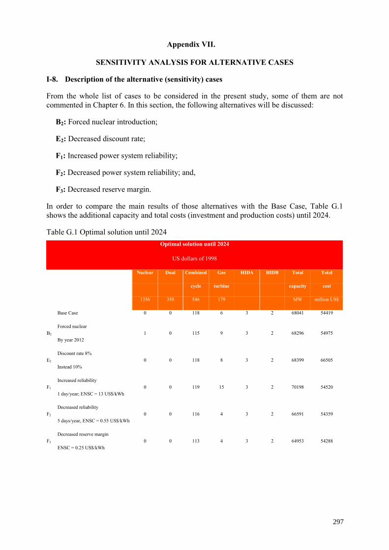
Appendix VII.

SENSITIVITY ANALYSIS FOR ALTERNATIVE CASES

I-8. Description of the alternative (sensitivity) cases

From the whole list of cases to be considered in the present study, some of them are not commented in Chapter 6. In this section, the following alternatives will be discussed:

B2: Forced nuclear introduction;

E2: Decreased discount rate;

F1: Increased power system reliability;

F2: Decreased power system reliability; and,

F3: Decreased reserve margin.

In order to compare the main results of those alternatives with the Base Case, Table G.1 shows the additional capacity and total costs (investment and production costs) until 2024.

Table G.1 Optimal solution until 2024 Optimal solution until 2024

US dollars of 1998

Nuclear Dual Combined Gas HIDA HIDB Total Total

cycle turbine capacity cost

1356 350 546 179 MW million US$

Base Case 0 0 118 6 3 2 68041 54419

B2 Forced nuclear

By year 2012 1 0 115 9 3 2 68296 54975

E2 Discount rate 8%

Instead 10% 0 0 118 8 3 2 68399 66505


1 day/year; ENSC = 13 US$/kWh 0 0 119 15 3 2 70198 54520


5 days/year, ENSC = 0.55 US$/kWh 0 0 116 4 3 2 66591 54359


ENSC = 0.25 US$/kWh 0 0 113 4 3 2 64953 54288

297

In Alternative B2, one forced nuclear power plant of 1 356 MW is assumed with the objective to see possible non-economic advantages of an additional nuclear power plant and its impacts on the system cost. It may be noted that the inclusion of a new nuclear power plant in 2012 reduces the number of combined cycle units of 546 MW, i.e., in this alternative the number of new combined cycle units is 115 compared with 118 in the Base Case whereas the capacity of gas turbines units of 179 MW is increased with 3 new gas turbine units. The total discounted cost (investment and system operation cost) increases to 54.975 billion dollars, because the investment increases to 10.272 and the operation expenditures (fuel and O&M cost) have a slight decrease to 44.702 billion dollars. In Alternative E2, the impact of the discount rate of 8% is not significant in the type and number of units to be installed, which are almost the same as in the Base Case - this alternative requires 8 gas turbine units of 179 MW instead of 6 units. Due to the discount rate of 8% the total discounted cost increases substantially to 66.505 billion dollars, 11.604 for investment and 54.900 for operation costs.

In order to increase the system reliability, Alternative F1 assumes the LOLP of 1 day per year instead of 3 days per year in the Base Case. The cost of ENS equals 13 US$/kWh instead of 1.5 US$/kWh with the objective to obtain the required LOLP of 1 day per year. In this condition the system requires 119 combined cycle units of 546 MW (64 974 MW) and 115 gas turbine units of 179 MW (2 685 MW). The total discounted cost has just a slight increase to 54.520 billion dollars, 9.682 for investment and 44.837 for operation expenditures.

On the other hand, to decrease the system reliability in Alternative F2, a LOLP of 5 days per year, instead of 3 days per year, as in the Base Case, is assumed. In this case, the cost of ENS equals to 0.55 US$/kWh instead of 1.5 US$/kWh. The optimal solution requires 116 combined cycle units of 546 MW (63 336 MW) and 4 gas turbine units of 179 MW (716 MW). The total cost decreases to 54.359 billion dollars, because the investment decreases to 9.468 while the operation and maintenance expenditures increases very little to 44.890 million dollars.

Finally in Alternative F3, it is assumed that the cost of ENS is 0.25 US$/kWh in order to decrease the reserve margin of the power system. The system requires the installation of 113 combined cycle units of 546 MW (61 698 MW) and 4 gas turbine units of 179 MW (716 MW). Compared with the Base Case, the system reserve margin obtained in this alternative is lower.

298

Appendix VIII.

ENERGY SYSTEM DIVERSITY

I-9. Measuring energy system diversity

Once the most economic expansion scenario is defined, it should be examined in terms of diversity. Is diversity good for the system or is it more economic to leave the system as it is? To answer this question one should first determine the value of diversity and verify if it is positive or negative. There are two objectives that are satisfied by a scenario with higher diversity than the Base Case, that is:

(1) There is a coverage in case of interruption of supply, like a oil shock or a future gas shock; and,

(2) There is a coverage to the high “volatility” of oil or gas prices in the future.

In the first case, the cost to the economy should be evaluated in terms of the energy non-served and how fast we can change to other technological options. The second case has been studied by means of the “portfolio theory” and the conclusions are that diversity is good if the resulting covariance is not positive for the optimal mix. It simply reflects the idea of not putting all the eggs in one basket. However if all energy prices will change following the same pattern, then diversity is not useful, unless we have domestic energy resources that we can develop soon. In this latter case diversity with non-fossil fuels such as nuclear or renewable is better than diversity with fossil fuels.

Once the diversity analysis is made, it has to be decided if the government should internalize this security externality, if the price paid to obtain this diversity is lower than the cost of these major disruptions e.g. it will be like the payment of some kind of insurance. After this study the government has to look at other options like the possibility of establishing stocks, the diversification of suppliers and supply contracts and plant/fuel substitutions. The cost of these options should be compared. Also the level of risk should be evaluated and defined as a policy to be followed by the country. In cases of a high degree of competition in the energy market the cost may be lower, but the level of risk will increase.

A diversity Index developed by Stirling was used to describe the diversity of the scenarios and was included in the DAM analysis. The Stirling Index was used as an indicator of energy supply diversity. The Index was calculated for the mix of the capacity resulting in the end year of the study for the selected expansions using the formula:

∑−=i

),(plnpH ii

where pi represents the proportion of installed capacity i in the total supply mix.

There are two problems in using this Index, one is to decide if we want to use it in terms of energy supplied by different fuels or in terms of installed capacity in the electric system. We believe that the Index will better express diversity in terms of capacity because the energy supplied depends on other factors like the level of demand, the power dispatching and the margin of reserve; while installed capacity will define the true mix of the system. The other problem is how to determine the weight or value of one unit of diversity expressed by this Index, in order to introduce it in the DAM study.

299

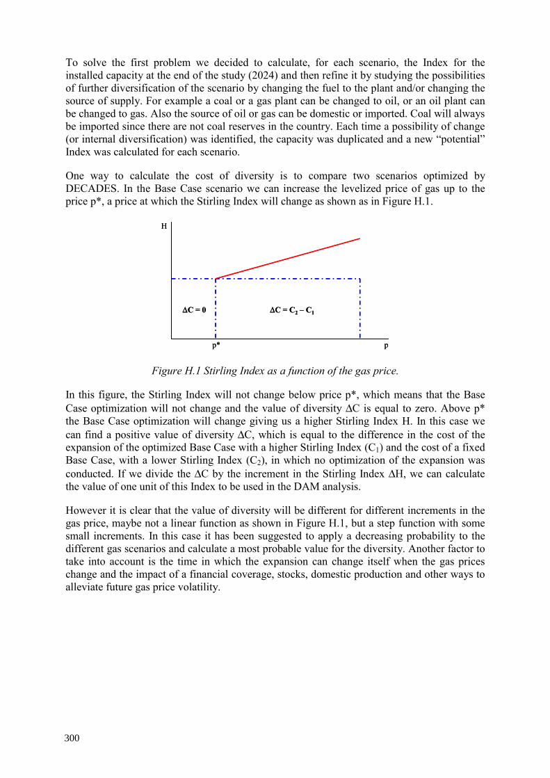
To solve the first problem we decided to calculate, for each scenario, the Index for the installed capacity at the end of the study (2024) and then refine it by studying the possibilities of further diversification of the scenario by changing the fuel to the plant and/or changing the source of supply. For example a coal or a gas plant can be changed to oil, or an oil plant can be changed to gas. Also the source of oil or gas can be domestic or imported. Coal will always be imported since there are not coal reserves in the country. Each time a possibility of change (or internal diversification) was identified, the capacity was duplicated and a new “potential” Index was calculated for each scenario.

One way to calculate the cost of diversity is to compare two scenarios optimized by DECADES. In the Base Case scenario we can increase the levelized price of gas up to the price p*, a price at which the Stirling Index will change as shown as in Figure H.1.

∆C = 0 ∆C = C2 – C1

p* p

H

∆C = 0 ∆C = C2 – C1

p* p

H

Figure H.1 Stirling Index as a function of the gas price.

In this figure, the Stirling Index will not change below price p*, which means that the Base Case optimization will not change and the value of diversity ∆C is equal to zero. Above p* the Base Case optimization will change giving us a higher Stirling Index H. In this case we can find a positive value of diversity ∆C, which is equal to the difference in the cost of the expansion of the optimized Base Case with a higher Stirling Index (C1) and the cost of a fixed Base Case, with a lower Stirling Index (C2), in which no optimization of the expansion was conducted. If we divide the ∆C by the increment in the Stirling Index ∆H, we can calculate the value of one unit of this Index to be used in the DAM analysis.

However it is clear that the value of diversity will be different for different increments in the gas price, maybe not a linear function as shown in Figure H.1, but a step function with some small increments. In this case it has been suggested to apply a decreasing probability to the different gas scenarios and calculate a most probable value for the diversity. Another factor to take into account is the time in which the expansion can change itself when the gas prices change and the impact of a financial coverage, stocks, domestic production and other ways to alleviate future gas price volatility.

300

REFERENCES

[1] CRISTERNA, R, Cross border electricity trade opportunities, 2nd International Symposium on World Energy Systems, Monterrey, Nuevo León, Mexico (2000).

[2] Proyecciones de Demanda de Energía en el Mercado Mexicano, 1996–2020 (HOUD & TRAN), Instituto Mexicano del Petróleo, México (2001).

[3] QUINTANILLA, J., Proyecciones de Demanda de Energía y Emisiones Asociadas, 2000–2010, Dirección General de Servicios de Cómputo Académico y Programa Universitario de Energía, UNAM, México (1999).

[4] QUINTANILLA, J., ET. AL., Uso Masivo de la Energía Solar en Sustitución de Combustibles Fósiles en la Zona Metropolitana del Valle de México (Sectores Residencial, Hospitalario, Hotelero y de Baños Públicos), DGSCA-UNAM, PUE-UNAM, Comisión Ambiental Metropolitana y World Bank, México (2000).

[5] Prospectiva del Sector Eléctrico, 2000-2009, Secretaría de Energía, México (2000). [6] Ökoinventare von Energiesystemen, Project-und Studienfonds der Elektrizitätswirt-

schaft, Budesamt für Energiewirtschaft (BEW), PSEL-LCA (1996). [7] US ENVIRONMENTAL PROTECTION AGENCY Air Pollution Emission Factors,

Vol. I, Stationary Point and Area Sources, AP-42, 5th edition (1996). [8] US ENVIRONMENTAL PROTECTION AGENCY: Air Pollution Emission

Factors, Mobile Sources, AP-42, 5th edition (1996).

301

ACRONYMS AND ABBREVIATIONS

ABWR Advanced Boiling Water Reactor

AP42 Compilation of Air Pollutant Emission Factors

Ar Argon

Ba Barium

BALANCE Energy Supply and Demand Analysis Module of ENPEP

BWR Boiling Water Reactor

C Carbon

CC54 Natural gas combined cycle unit with a capacity of 546 MW

CCGT Combined Cycle Gas Turbine

Ce Cerium

CEEESA Center for Energy, Environmental, and Economic Systems Analysis

CH4 Methane

CO Carbon Monoxide

Co Cobalt

CO2 Carbon Dioxide

CO2-biomass Carbon Dioxide from biomass

COGEN WASP Configuration Generator

COPAR Costs and Parameters of Reference for the Formulation of Investment Projects in the Power Sector

Cr Chromium

Cs Cesium

CSDB Country Specific Databases

Cu Copper

DAM Decision Analysis Module of ENPEP for Windows

DAM Decision Analysis Module of DECADES for Windows

DECADES Databases and MEthodologies for Comparative Assessment of Different Energy Sources for Electricity Generation

DECPAC DECADES analytical software for analysis and comparison of costs and environmental burdens

DGSCA-UNAM Dirección General de Servicios de Cómputo Académico-UNAM

DMS Database Management System

DOE U. S. Department of Energy

DYNPRO WASP Dynamic Programming Optimization

EC European Union

ENPEP Energy and Power Evaluation Program

303

ENS energy not served

FGD flue gas desulphurization

FIXSYS WASP fixed system description

FO fuel oil

GDP gross domestic product

GHG greenhouse gasses

GTMax Generation and Transmission Maximization Model

H Stirling Index

H2S Hydrogen sulfide

HCl Hydrogen Chloride

HEIES impacts database

HF Hydrogen Fluoride

HLW high level waste

I Iodine

ICARUS Investigating Costs and Reliability in Utility Systems

IIE Electrical Research Institute

IMPACTS Environmental Impact Module of ENPEP for Windows

IPCC Intergovernmental Panel on Climate Change

IPPS independent power producers

IS interconnected system

Kr Krypton

La Lanthanum

LCC limited combined cycle

LDC load duration curve

LMLW low/medium level waste

LNG liquefied natural gas

LOAD load module of ENPEP for Windows

LOADSY WASP load system description

LOLP loss of load probability

LPG liquefied petroleum gas

LYFC Light and Power Company for the Center

M million (mega)

MACRO-E macroeconomic module of ENPEP for Windows

MAED model for analysis of energy demand

MBq Mega Becquerel

304

MERSIM WASP merge and simulate

Mn Manganese

MODEMA MOdelo de DEMAnda de Energía (Energy Demand Model)

N135 advanced boiling water reactor with a capacity of 1,356 MW

N2O Nitrous Oxides

N655 Boiling water reactor with a capacity of 654 MW

Nb Niobium

ND35 Dual fuel unit with desulphurization and a capacity of 350 MW

NES National Electric System

NG natural gas

NGI National Interconnected Grid

NGL Natural Gas Liquids

NH3 Ammonia

NMTOC non-methane total organic compounds

NMVOC non-methane volatile organic compounds

NOC net overnight cost

NOM-085-ECOL-1994 Mexican standard that regulates smoke, total suspended particles, sulfur and nitrogen oxides from fixed sources that use fossil fuels

NOX Nitrogen Oxides

NPV net present value

NREL National Renewable Energy Laboratory

NRS national refinery system

O&M Operation and Maintenance

OECD Organization for Economic Cooperation and Development

Pb Lead

PCVAL PC-Valoragua

PEP PEMEX-Exploration and Production

PGPB PEMEX- Gas and Basic Petrochemicals

PIE Productores Independientes de Electricidad (Electricity Independent Producers)

PM particulate matter

ppm parts per million

PPQ PEMEX-Petrochemicals

PR PEMEX-Refining

PUE-UNAM Programa Universitario de Energía-UNAM

PV Photovoltaic

305

REMERSIM WASP Re-Merge and Simulate

REPROBAT WASP Report Writer in a Batched Environment

RTDB reference technology database

Ru Ruthenium

Sb Antimony

SENER Ministry of Energy

SO2 Sulfur Dioxide

SOX Sulfur Oxides

SPNRES spinning reserve

Sr Strontium

SWU separative working units

T&D transmission and distribution

T179 natural gas simple cycle unit with a capacity of 179 MW

TFC total final energy consumption

TOC total organic compounds

TPES total primary energy supply

TRAN transport data base for Mexico

TSP total suspended particles

UED useful energy demand

V Vanadium

VALORAGUA Hydro Simulation Model

VARSYS WASP Variable System Description

VOC Volatile Organic Compounds

WASP Wien Automatic Planning Package

WFGD Wet Flue Gas Desulphurization

Xe Xenon

Zn Zinc

306

UNITS OF MEASURE

% p.a. per cent per year

$ US dollar

$/kW US Dollars per kilowatt

$/MMbtu US Dollars per million Btu

$/ MW·h US Dollars per megawatt hour

ºC degree Celsius

bcm billion cubic meters

boe barrel of oil equivalent

BTU British Thermal Unit

cal/cm2 calorie per square centimeter

cbm cubic meters

g gram

GW Gigawatt

GW·h Gigawatt hour

kcal kilocalorie

kcal/kg kilocalorie per kilogram

kcal/ kW·h kilocalorie per kilowatt hour

kg kilogram

km kilometer

km2 square kilometer

mth month

MW(d) Megawatt day

Mw(e) Megawatt electric

kW(e) kilowatt electric

kW·h kilowatt hour

kW·h /m2 kilowatt hour per square meter

l liter

J Joule

h hour

yr year

m meter

m/s meter per second

m3 cubic meter

mm millimeter

307

Mt million metric tons

Mt/yr million metric tons per year

Mtoe million tons of oil equivalent

MJ Megajoule

Mg milligram

ng nanogram

GJ Gigajoule

MW Megawatt

MW(e) Megawatt electric

MW(th) Megawatt thermal

PJ Petajoules

ton metric ton

t/yr metric ton per year

toe ton of oil equivalent

TJ Terajoule

TW·h Terawatt-hours

Watt/m2 Watt per square meter

Wh Watt hour

kboe 1000 barrels of oil equivalent

kt 1000 tons

ktoe 1000 tons of oil equivalent

toe/US$1,000 ton of oil equivalent per 1,000 US Dollars

US$ US Dollars (all costs in this report are in constant US$2000)

308

CONTRIBUTORS TO DRAFTING AND REVIEW

Aguilar Alejandre, V. Secretaría de Energía

Cadena Vargas, H. Comisión Federal de Electricidad

Conde Alvarez, L.A. Instituto Nacional de Ecología

Fernández Velázquez, J. Comisión Federal de Electricidad

Guenter. C. Center for Energy, Environmental, and Economic Systems Analysis of Argonne National Laboratory

Ibars Hernández, E. Comisión Federal de Electricidad

Ismael, C. Unidad de Plantation Minero-Energetica, Colombia

Jiménez Lerma. I. Comisión Federal de Electricidad

Kee-Yung Nam International Atomic Energy Agency

Kononov, S. International Atomic Energy Agency

Martín del Campo Márquez, C Facultad de Ingeniería, UNAM

Mar Juárez, E. Instituto Mexicano del Petróleo

Ortega Carmona, R. Facultad de Ingeniería, UNAM

Rodríguez García, A. Instituto de Investigaciones Eléctricas

Serrato Angeles. G. Facultad de Ingeniería, UNAM

Quintanilla Martínez, J. Dirección General de Servicios de Cómputo Académico, UNAM, Programa Universitario de Energía, UNAM

309

Documents

Comparative assessment of energy options and strategies in ... · IAEA-TECDOC-1469 Comparative assessment of energy options and strategies in Mexico until 2025 Final report of a coordinated