2.3 Compactness

2.3. COMPACTNESS 1

2.3 Compactness

Recall that Bolzano-Weierstrass Theorem asserts that every sequence in a closed boundedinterval has a convergent subsequence in this interval. The result still holds for all closed,bounded sets in Rn. In general, a set E ⇢ (X, d) is compact if every sequence has a con-vergent subsequence with limit in E. This property is also called sequentially compactto stress that the behavior of sequences is involved in the definition. The space (X, d)is called a compact space is X is a compact set itself. According to this definition,every interval of the form [a, b] is compact in R and sets like [a1, b1]⇥ [a2, b2]⇥ · · · [a

n

, bn

]and B

r

(x) are compact in Rn under the Euclidean metric. In a general metric space, thenotion of a bounded set makes perfect sense. Indeed, a set A is called a bounded set ifthere exists some ball B

r

(x) for some x 2 X and r > 0 such that A ⇢ Br

(x). Now we in-vestigate the relation between a compact set and a closed bounded set. First of all, we have

Proposition 2.1. Every compact set in a metric space is closed and bounded.

Proof. Let K be a compact set. To show that it is closed, let {xn

} ⇢ K and xn

! x0.We need to show that x0 2 K. As K is compact, there exists a subsequence {x

n

j

} ⇢ Kconverging to some z in K. By the uniqueness of limit, we have x0 = z 2 K, so x0 2 Kand K is closed.

Next, we show that K is bounded. If on the contrary it is not, for a fixed point w,K is not contained in the balls B

n

(w) for all n. Picking xn

2 K \ Bn

(w), we obtain asequence {x

n

} satisfying d(xn

, w) ! 1 as n ! 1. By the compactness of K, there isa subsequence {x

n

j

} converging to some z in K. Therefore, for all su�ciently large nj

,xn

j

2 B1(z). By the triangle inequality,

d(xn

j

, w) d(xn

j

, w) + d(w, z)

1 + d(x1, z) < 1 ,

contradicting d(xn

j

, w) ! 1 as nj

! 1. Hence K must be bounded.

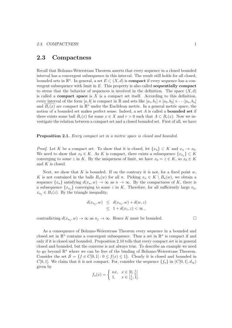
As a consequence of Bolzano-Weierstrass Theorem every sequence in a bounded andclosed set in Rn contains a convergent subsequence. Thus a set in Rn is compact if andonly if it is closed and bounded. Proposition 2.10 tells that every compact set is in generalclosed and bounded, but the converse is not always true. To describe an example we needto go beyond Rn where we can be free of the binding of Bolzano-Weierstrass Theorem.Consider the set S = {f 2 C[0, 1] : 0 f(x) 1}. Clearly it is closed and bounded inC[0, 1]. We claim that it is not compact. For, consider the sequence {f

n

} in (C[0, 1], d1)given by

fn

(x) =

⇢

nx, x 2 [0, 1n

]1, x 2 [ 1

n

, 1].

2

{fn

(x)} converges pointwisely to the function f(x) = 1, x 2 (0, 1] and f(0) = 0 which isdiscontinuous at x = 0, that is, f does not belong to C[0, 1]. If {f

n

} has a convergentsubsequences, then it must converge uniformly to f . But this is impossible because theuniform limit of a sequence of continuous functions must be continuous. Hence S cannotbe compact. In fact, a remarkable theorem in functional analysis asserts that the closedunit ball in a normed space is compact if and only if the normed space if and only if thenormed space is of finite dimension.

Since convergence of sequences can be completely described in terms of open/closedsets, it is natural to attempt to describe the compactness of a set in terms of these newnotions. The answer to this challenging question is a little strange at first sight. Let usrecall the following classical result:

Heine-Borel Theorem. Let {Ij

}1j=1 be a family of open intervals satisfying

[a, b] ⇢1[

j=1

Ij

.

There is always a finite subfamily {Ij1 , · · · , Ij

K

} such that

[a, b] ⇢K

[

k=1

Ij

k

.

This property is not true for open (a, b). Indeed, the intervals {(a+ 1/j, b� 1/j)} satisfy(a, b) ⇢

S

j

(a + 1/j, b � 1/j) but there is no finite subcover. It is a good exercise toshow that Heine-Borel Theorem is equivalent to Bolzano-Weierstrass Theorem. (WhenI was an undergraduate in this department in 1974, we were asked to show this equiva-lence, together with the so-called Nested Interval Theorem, in a MATH2050-like course.)This equivalence motivates how to describe compactness in terms of the language ofopen/closed sets.

We introduce some terminologies. First of all, an open cover of a subset E in ametric space (X, d) is a collection of open sets {G

↵

},↵ 2 A, satisfying E ⇢S

↵2A G↵

.A set E ⇢ X satisfies the finite cover property if whenever {G

↵

},↵ 2 A, is an opencover of E, there exist a subcollection consisting of finitely many G

↵1 , . . . , G↵

N

such thatE ⇢

S

N

j=1 G↵

j

. (“Every open cover has a finite subcover.”) A set E satisfies the finite in-tersection property if whenever {F

↵

} ,↵ 2 A, are relatively closed sets in E satisfyingT

N

j=1 F↵

j

6= � for any finite subcollection F↵

j

,T

↵2A F↵

6= �. Here a set F ⇢ E is relativelyclosed means F is closed in the subspace E. We know that it implies F = A\E for someclosed set A. Therefore, when E is closed, a relatively closed subset is also closed. (In thissemester I have skipped the discussion on subspace and relative openness and closedness.You may simply ignore the di↵erence between a closed set and a relatively closed set inthese notes.)

2.3. COMPACTNESS 3

Proposition 2.2. A closed set has the finite cover property if and only if it has the finite

intersection property.

Proof. Let E be a non-empty closed set in (X, d).

)) Suppose {F↵

}, F↵

closed sets contained in E, satisfiesT

N

j=1 F↵

j

6= � for any finitesubcollection but

T

↵2A F↵

= �. As E is closed, each F↵

is closed in X, and

E = E \\

↵2A

F↵

=[

↵2A

(E \ F 0↵

) ⇢[

↵2A

F 0↵

.

By the finite covering property we can find ↵1, . . . ,↵N

such that E ⇢S

N

j=1 F0↵

j

, but then

� = E \ E � E \S

N

1 F 0↵

j

=T

N

j=1 F↵

j

, contradiction holds.

() If E ⇢S

↵2A G↵

but E (S

N

j=1 G↵

j

for any finite subcollection of A, then

� 6= E \N

[

j=1

G↵

j

=N

\

j=1

�

E \G↵

j

�

which impliesT

↵2A�

E \ G↵

�

6= � by the finite intersection property. Note that each

E \ G↵

j

is closed. Using ET

�

S

↵2A G↵

�0=

T

↵2A�

E \ G↵

�

, we have E (S

↵2A G↵

,contradicting our assumption.

Remark 2.1. It is no hard to see that every closed subset of a closed set satisfies thefinite cover property/finite intersection property if the closed set itself satisfies the sameproperty.

Proposition 2.3. Let E be compact in a metric space. For each ↵ > 0, there exist finitelymany balls B

↵

(x1), . . . , B↵

(xN

) such that E ⇢S

N

j=1 B↵

(xj

) where xj

, 1 j N, are in

E.

Proof. Pick B↵

(x1) for some x1 2 E. Suppose E \ B↵

(x1) 6= �. We can find x2 /2 B↵

(x1)so that d(x2, x1) � ↵. Suppose E \

�

B↵

(x1)S

B↵

(x2)�

is non-empty. We can find x3 /2B

↵

(x1)S

B↵

(x2) so that d(xj

, x3) � ↵, j = 1, 2. Keeping this procedure, we obtain asequence {x

n

} in E such that

E \n

[

j=1

B↵

(xj

) 6= � and d(xj

, xn

) � ↵, j = 1, 2, . . . , n� 1.

By the compactness of E, there exists�

xn

j

and x 2 E such that xn

j

! x as j ! 1.But then d(x

n

j

, xn

k

) < d(xn

j

, x)+d(xn

k

, x) ! 0, contradicting d(xj

, xn

) � ↵ for all j < n.

Hence one must have E \S

N

j=1 B↵

(xj

) = � for some finite N .

4

Sometimes the following terminology is convenient. A set E is called totally boundedif for each " > 0, there exist x1, · · · , xn

2 X such that E ⇢ [n

k=1B"

(xk

). Proposition 2.12simply states that every compact set is totally bounded. We will use this property of acompact set again in the next chapter.

Theorem 2.4. Let E be a closed set in (X, d). The followings are equivalent:

(a) E is compact;

(b) E satisfies the finite cover property; and

(c) E satisfies the finite intersection property.

Proof. The equivalence between (b) and (c) has been established in Proposition 2.11.

(a)) (b). Let {G↵

} be an open cover of E without finite subcover and we will draw acontradiction. By Proposition 2.12, for each k � 1, there are finitely many balls of radius1/k covering E. We can find a set B1/k \E (suppress the irrelevant center) which cannotbe covered by finitely many members in {G

↵

}. Pick xk

2 B1/k \ E to form a sequence.By the compactness of E, we can extract a subsequence {x

k

j

} such that xk

j

! x for somex0 2 E. Since {G

↵

} covers E, there must be some G↵1 that contains x0. As G↵1 is open

and the radius of B1/kj

tends to 0, we deduce that, for all su�ciently large kj

, B1/kj

\E iscontained in G

↵1 . In other words, G↵1 forms a single subcover of B1/k \E, contradicting

our choice of B1/kj

\ E. Hence (b) must be valid.

(b), (c)) (a). Let {xn

} be a sequence in E. Without loss of generality we may assumethat it contains infinitely many distinct points, otherwise the conclusion is obvious. LetA denote the set consisting of all points in this sequence. All balls of radius 1 cover Xand hence A. By the finite cover property (see Remark 2.1) there is a finite cover of A.We can pick one B1 such that B1 \ A contains infinitely many points from A. Next, allballs of radius 1/2 cover B1 \ A. By the same reasoning, we let B1/2 be a ball of radius1/2 such that B1/2 \ B1 \ A contains infinitely many points from A. By repeating thisprocess, we obtain a sequence of balls, {B1/k}, one of each of radius 1/k, such that thereare infinitely many points of A inside C

k

= B1/k \B1/(k�1) · · ·\B1\A. Pick a point fromeach C

k

to form a subsequence {zk

} of {xn

}. (Here we use the fact that there are infinitelymany points of A in C

k

to guarantee the existence of the subsequence.) Observing thatC

k

is descending and so enjoys the finite intersection property,T

k

Ck

is non-empty. Letz be a point in this common intersection. (In fact, there is exactly one point in thiscommon intersection, but we do not need this fact.) As the radius of B1/k tending to 0,{z

k

} converges to z. We have shown that E is compact.

In the proof of the following result, we illustrate how to prove the same statement byusing the subsequence approach and the finite cover approach.

2.3. COMPACTNESS 5

Proposition 2.5. Let K be a compact set and G be an open set, K ⇢ G, in the metric

space (X, d). Then

dist (K, @G) > 0,

where dist (A,B) = inf{d(x, y) : x 2 A, y 2 B}.

Proof. First proof: Suppose on the contrary that dist (K, @G) = 0. By the definition ofthe distance between two sets, there are {x

n

} ⇢ K and {yn

} ⇢ @G such that d(xn

, yn

) !0. By the compactness of K, there exists a subsequence {x

n

j

} and x⇤ 2 K such thatxn

j

! x⇤. From d(x⇤, yn

j

) d(xn

j

, yn

j

) + d(x⇤, xn

j

) ! 0 we see that x⇤ 2 @G (theboundary of a set is always closed). But then G \ @G is non-empty, which is impossibleas G is open. So dist (K, @G) > 0.

Second proof: For x 2 K, we claim that d(x, @G) > 0. For, if d(x, @G) = 0, thereexists {y

n

} ⇢ @G, d(x, yn

) ! 0, but then x belongs to @G. As the boundary of aset is always a closed set, x 2 @G contradicting x 2 G. So d(x, @G) > 0. Due thecontinuity of x 7! d(x, @G), we can find a small number ⇢

x

> 0 such that dist (y, @G) �d(x, @G)/2 > 0 for all y 2 B

⇢

x

(x). That is, dist(B⇢

x

(x), @G) � d(x, @G)/2. The collectionof all balls B

⇢

x

(x), x 2 K, forms an open cover of K. Since K is compact, there existx1, · · · , xN

, such that B⇢

x

j

(xj

), j = 1, · · · , N, form a finite subcover of K. Taking � =min{d(x1, @G)/2, · · · , d(x

N

, @G)/2}, we conclude dist(K, @G) � dist([j

B⇢

j

(xj

), @G) �� > 0.

We finally note

Proposition 2.6. Let E be a compact set in (X, d) and F : (X, d) ! (Y, ⇢) be continuous.Then f(E) is a compact set in (Y, ⇢).

Proof. Let {yn

} be a sequence in f(E) and let {xn

} be in E satisfying f(xn

) = yn

for alln. By the compactness of E, there exist some {x

n

j

} and x in E such that xn

j

! x asj ! 1. By the continuity of f , we have y

n

j

= f(xn

j

) ! f(x) in f(E). Hence f(E) iscompact.

Can you prove this property by using the finite cover property of compact sets?

There are several fundamental theorems which hold for continuous functions definedon a closed, bounded set in the Euclidean space. Notably they include

• A continuous function on a closed, bounded set is uniformly continuous; and

• A continuous function on a closed, bounded set attains its minimum and maximumin the set.

Although they may no longer hold on arbitrary closed, bounded sets in a general metricspace, they continue to hold when the sets are strengthened to compact ones. The proofsare very much like in the finite dimensional case. I leave them as exercises.

2.6. THE INVERSE FUNCTION THEOREM 1

2.6 The Inverse Function Theorem

The Inverse Function Theorem and Implicit Function Theorem play a fundamental role inanalysis and geometry. They illustrate the principle of linearization which is ubiquitousin mathematics. We learned these theorems in advanced calculus but the proofs were notemphasized. Now we fill out the gap. Adapting the notations in advanced calculus, apoint x = (x1, x2, · · · , xn) ∈ Rn is sometimes called a vector and we use |x| instead of‖x‖2 to denote its Euclidean norm in this section.

All is about linearization. Recall that a real-valued function on an open interval I isdifferentiable at some x0 ∈ I if there exists some a ∈ R such that

limx→x0

∣∣∣f(x)− f(x0)− a(x− x0)x− x0

∣∣∣ = 0.

In fact, the value a is equal to f ′(x0), the derivative of f at x0. We can rewrite the limitabove using the little o notation:

f(x0 + z)− f(x0) = f ′(x0)z + ◦(z), as z → 0.

Here ◦(z) denotes a quantity satisfying limz→0 ◦(z)/|z| = 0. The same situation carriesover to a real-valued function f in some open set in Rn. A function f is called differentiableat x0 in this open set if there exists a vector a = (a1, · · · , an) such that

f(x0 + x)− f(x0) =n∑j=1

ajxj + ◦(z) as x→ 0.

Note that here x0 = (x10, · · · , xn0 ) is a vector. Again one can show that the vector a isuniquely given by the gradient vector of f at x0

∇f(x0) =

(∂f

∂x1(x0), · · · ,

∂f

∂xn(x0)

).

More generally, a map F from an open set in Rn to Rm is called differentiable at a pointx0 in this open set if each component of F = (f 1, · · · , fm) is differentiable. We can writethe differentiability condition collectively in the following form

F (x0 + x)− F (x0) = DF (x0)x+ o(x), (2.3)

where DF (x0) is the linear map from Rn to Rm given by

(DF (x0)z)i =n∑j=1

aij(x0)xj, i = 1, · · · ,m,

where(aij)

=(∂f i/∂xj

)is the Jabocian matrix of f . (2.3) shows near x0, that is, when

x is small, the function F is well-approximated by the linear map DF (x0) up to the

2

constant F (x0) as long as DF (x0) is nonsingular. It suggests that the local informationof a map at a differentiable point could be retrieved from its a linear map, which is mucheasier to analyse. This principle, called linearization, is widely used in analysis. TheInverse Function Theorem is a typical result of linearization. It asserts that a map islocally invertible if its linearization is invertible. Therefore, local bijectivity of the map isensured by the invertibility of its linearization. When DF (x0) is not invertible, the firstterm on the right hand side of (2.3) may degenerate in some or even all direction so thatDF (x0)x cannot control the error term ◦(|z|). In this case the local behavior of F maybe different from its linearization.

Theorem 2.1 (Inverse Function Theorem). Let F : U → Rn be a C1-map where Uis open in Rn and x0 ∈ U . Suppose that DF (x0) is invertible.

(a) There exist open sets V and W containing x0 and F (x0) respectively such that therestriction of F on V is a bijection onto W with a C1-inverse.

(b) The inverse is Ck when F is Ck, 1 ≤ k ≤ ∞, in V .

A map from some open set in Rn to Rm is Ck, 1 ≤ k ≤ ∞, if all its components belongto Ck. It is called a C∞-map or a smooth map if its components are C∞. Similarly, amatrix is Ck or smooth if its entries are Ck or smooth accordingly.

The condition that DF (x0) is invertible, or equivalently the non-vanishing of thedeterminant of the Jacobian matrix, is called the nondegeneracy condition. Withoutthis condition, the map may or may not be local invertible, see the examples below.Nevertheless, it is necessary for the differentiability of the local inverse. At this point, letus recall the general chain rule.

Let G : Rn → Rm and F : Rm → Rl be C1 and their composition H = F ◦ G :Rn → Rl is also C1. We compute the first partial derivatives of H in terms of the partialderivatives of F and G. Letting G = (g1, · · · , gm), F = (f1, · · · , fl) and H = (h1, · · · , hl).From

hk(x1, · · · , xn) = fk(g1(x), · · · , gm(x)), k = 1, · · · , l,

we have∂hk∂yi

=n∑i=1

∂fk∂xi

∂gi∂xj

.

Writing it in matrix form we have

DF (G(x))DG(x) = DH(x).

When the inverse is differentiable, we may apply this chain rule to differentiate therelation F−1(F (x)) = x to obtain

DF−1(y0) DF (x0) = I , y0 = F (x0),


where I is the identity map. We conclude that

DF−1(y0) =(DF (x0)

)−1,

in other words, the matrix of the derivative of the inverse map is precisely the inversematrix of the derivative of the map. We conclude that in order to have a differentiableinverse near x0, DF (x0) must be invertible.

Lemma 2.1. Let A be a linear map from Rn to itself given by

(Ax)i =n∑j=1

aijxj, i = 1, · · ·n.

Then|Az| ≤M(A) |z|, ∀z ∈ Rn,

where M(A) =√∑

i,j a2ij.

Proof. By Cauchy-Schwarz inequality,

|Ax|2 =∑i

(Ax)2i

=∑i

(∑j

aijxj)2

≤∑i

(∑j

a2ij)(∑

j

x2j)

= M(A)2 |x|2 .

Now we prove Theorem 2.19. Let x0 ∈ U and y0 = F (x0). We set F (x) = F (x+ x0)− y0in U = U − x0 so that F (0) = 0 and DF (0) = DF (x0). First we would like to show

that there is a unique solution for the equation F (x) = y for y near 0. We will use theContraction Mapping Principle to achieve our goal. After a further restriction on the sizeof U = U − x0, we may assume that F is C1 with DF (x) invertible at all x ∈ U . For a

fixed y, define the map in U by

T (x) = L−1(Lx− F (x) + y

)where L = DF (0). It is clear that any fixed point of T is a solution to F (x) = y. By thelemma,

|T (x)| 6 M(L−1) |F (x)− Lx− y|

6 M(L−1)(|F (x)− Lx|+ |y|

)≤ M(L−1)

(∣∣∣∣ˆ 1

0

(DF (tx)−DF (0))dt x

∣∣∣∣+ |y|),

4

where we have used the formula

F (x)−DF (0)x =

ˆ 1

0

d

dtF (tx)dt−DF (0)x =

ˆ 1

0

(DF (tx)−DF (0)

)dt x,

after using the chain rule to get

d

dtF (tx) = DF (tx) · x.

By the continuity of DF at 0, we can find a small ρ0 such that Bρ0(0) ⊂ U and

M(L−1)M(DF (x)−DF (0)) ≤ 1

2, ∀x ∈ Bρ0(0) . (2.4)

Then for for each y in BR(0), where R is chosen to satisfy M(L−1)R ≤ ρ0/2, by (2.4) wehave

|T (x)| ≤ M(L−1)

(ˆ 1

0

|(DF (tx)−DF (0))x|dt+ |y|)

≤ M(L−1)

(supt∈[0,1]

M(DF (tx)−DF (0))|x|+ |y|

)≤ 1

2|x|+M(L−1)|y|

≤ 1

2ρ0 +

1

2ρ0 = ρ0,

for all x ∈ Bρ0(0). We conclude that T maps Bρ0(0) to itself. Moreover, for x1, x2 inBρ0(0), we have

|T (x2)− T (x1)| =∣∣∣M(L−1)

(F (x2)− Lx2 − y

)− L−1

(F (x1)− Lx1 − y

)∣∣∣6 M(L−1)

∣∣∣F (x2)− F (x1)−DF (0)(x2 − x1)∣∣∣

6 M(L−1)

∣∣∣∣ˆ 1

0

DF (x1 + t(x2 − x1)) (x2 − x1)dt−DF (0)(x2 − x1)∣∣∣∣ ,

where we have used

F (x2)− F (x1) =

ˆ 1

0

d

dtF (x1 + t(x2 − x1))dt

=

ˆ 1

0

DF (x1 + t(x2 − x1))(x2 − x1)dt.

Using (2.4) we have,

|T (x2)− T (x1)| ≤1

2|x2 − x1|.


We have shown that T : Bρ0(0)→ Bρ0(0) is a contraction. By the Contraction MappingPrinciple, there is a unique fixed point for T , in other words, for each y in the ball BR(0)

there is a unique point x in Bρ0(0) solving F (x) = y. Defining G : BR(0)→ Bρ0(0) ⊂ U

by setting G(y) = x, G is inverse to F .

Next, we claim that G is continuous. In fact, for G(yi) = xi ∈ BR(0), i = 1, 2, (notto be mixed up with the xi above),

|G(y2)− G(y1)| = |x2 − x1|= |T (x2)− T (x1)|

≤ M(L−1)(∣∣∣F (x2)− F (x1)− L(x2 − x1)

∣∣∣+ |y2 − y1|)

≤ M(L−1)

(∣∣∣∣ˆ 1

0

(DF ((1− t)x1 + tx2)−DF (0)

)dt(x2 − x1)

∣∣∣∣+ |y2 − y1|)

≤ 1

2|x2 − x1|+M(L−1)|y2 − y1|

=1

2|G(y2)− G(y1)|+M(L−1)|y2 − y1|,

where (2.4) has been used. We deduce

|G(y2)− G(y1)| 6 2M(L−1)|y2 − y1| , (2.5)

that’s, G is Lipschitz continuous on BR(0).

Finally, let’s show that G is a C1-map in BR(0). In fact, for y1, y1 + y in BR(0), using

y = (y1 + y)− y1= F (G(y1 + y))− F (G(y1))

=

ˆ 1

0

DF (G(y1) + t(G(y1 + y)− G(y1))dt (G(y1 + y)− G(y1)),

we haveG(y1 + y)− G(y1) = (DF )−1(G(y1))y +R,

where R is given by

(DF )−1(G(y1))

ˆ 1

0

(DF (G(y1))−DF (G(y1)+t(G(y1+y)−G(y1))

)(G(y1+y)−G(y1))dt.

As G is continuous and F is C1, we have

G(y1 + y)− G(y1)− (DF )−1(G(y1))y = ◦(1)(G(y1 + y)− G(y1))

for small y. Using (2.5), we see that

G(y1 + y)− G(y1)− (DF )−1(G(y1))y = ◦(y) ,

6

as |y| → 0. We conclude that G is differentiable with Jacobian matrix (DF )−1(G(y1)).

Going back to the original function, we see that G(y) = G(y−y0)+x0 is the C1-inverseto F from BR(y0) back to Bρ0(x0) ⊂ U .

After proving the differentiability of G, from the formula DF (G(y))DG(y) = I whereI is the identity matrix we see that DG(y) = (DF (G(y))−1 for y ∈ BR(0). From linearalgebra we know that each entry of DG(y) can be expressed as a rational function of theentries of the matrix of DF (G(y)). Consequently, DG(y) is Ck in y if DF (G(y)) is Ck

for 1 ≤ k ≤ ∞.

The proof of the Inverse Function Theorem is completed by taking W = BR(y0) andV = G(W ).

Example 2.1. The Inverse Function Theorem asserts a local invertibility. Even if thelinearization is non-singular everywhere, we cannot assert global invertibility. Let usconsider the switching between the cartesian and polar coordinates in the plane:

x = r cos θ, y = r sin θ .

The function F : (0,∞) × (−∞,∞) → R2 given by F (r, θ) = (x, y) is a continuouslydifferentiable function whose Jacobian matrix is non-singular except (0, 0). However, itis clear that F is not bijective, for instance, all points (r, θ + 2nπ), n ∈ Z, have the sameimage under F .

Example 2.2. An exceptional case is dimension one where a global result is available.Indeed, in Mathematical Analysis II we learned that if f is continuously differentiable on(a, b) with non-vanishing f ′, it is either strictly increasing or decreasing so that its globalinverse exists and is again continuously differentiable.

Example 2.3. Consider the map F : R2 → R2 given by F (x, y) = (x2, y). Its Jacobianmatrix is singular at (0, 0). In fact, for any point (a, b), a > 0, F (±

√a, b) = (a, b). We

cannot find any open set, no matter how small is, at (0, 0) so that F is injective. On theother hand, the map H(x, y) = (x3, y) is bijective with inverse given by J(x, y) = (x1/3, y).However, as the non-degeneracy condition does not hold at (0, 0) so it is not differentiablethere. In these cases the Jacobian matrix is singular, so the nondegeneracy condition doesnot hold. We will see that in order the inverse map to be differentiable, the nondegeneracycondition must hold.

Inverse Function Theorem may be rephrased in the following form.

A Ck-map F between open sets V and W is a “Ck-diffeomorphism” if F−1 exists and isalso Ck. Let f1, f2, · · · , fn be Ck-functions defined in some open set in Rn whose Jacobianmatrix of the map F = (f1, · · · , fn) is non-singular at some point x0 in this open set. ByTheorem 4.1 F is a Ck-diffeomorphism between some open sets V and W containing x0and F (x0) respectively. To every function Φ defined in W , there corresponds a function


defined in V given by Ψ(x) = Φ(F (x)), and the converse situation holds. Thus everyCk-diffeomorphism gives rise to a “local change of coordinates”.

Next we deduce Implicit Function Theorem from Inverse Function Theorem.

Theorem 2.2 (Implicit Function Theorem). Consider C1-map F : U → Rm whereU is an open set in Rn × Rm. Suppose that (x0, y0) ∈ U satisfies F (x0, y0) = 0 andDyF (x0, y0) is invertible in Rm. There exist an open set V1 × V2 in U containing (x0, y0)and a C1-map ϕ : V1 → V2, ϕ(x0) = y0, such that

F (x, ϕ(x)) = 0 , ∀x ∈ V1 .

The map ϕ belongs to Ck when F is Ck, 1 ≤ k ≤ ∞, in U . Moreover, if ψ is anotherC1-map in some open set containing x0 to V2 satisfying F (x, ψ(x)) = 0 and ψ(x0) = y0,then ψ coincides with ϕ in their common set of definition.

The notation DyF (x0, y0) stands for the linear map associated to the Jocabian matrix(∂Fi/∂yj(x0, y0))i,j=1,··· ,m where x0 is fixed. In general, a version of Implicit FunctionTheorem holds when the rank of DF at a point is m. In this case, we can rearrange theindependent variables to make DyF non-singular at that point.

Proof. Consider Φ : U → Rn ×Rm given by

Φ(x, y) = (x, F (x, y)).

It is evident that DΦ(x, y) is invertible in Rn × Rm when DyF (x, y) is invertible in Rm.By the Inverse Function Theorem, there exists a C1-inverse Ψ = (Ψ1,Ψ2) from some openW in Rn ×Rm containing Φ(x0, y0) to an open subset of U . By restricting W further wemay assume Ψ(W ) is of the form V1 × V2. For every (x, z) ∈ W , we have

Φ(Ψ1(x, z),Ψ2(x, z)) = (x, z),

which, in view of the definition of Φ, yields

Ψ1(x, z) = x, and F ((Ψ1(x, z),Ψ2(x, z)) = z.

In other words, F (x,Ψ2(x, z)) = z holds. In particular, taking z = 0 gives

F (x,Ψ2(x, 0)) = 0, ∀x ∈ V1 ,

so the function ϕ(x) ≡ Ψ2(x, 0) satisfies our requirement.

By restricting V1 and V2 further if necessary, we may assume the matrix

ˆ 1

0

DyF (x, y1 + t(y2 − y1)dt

8

is nonsingular for (x, y1), (x, y2) ∈ V1 × V2. Now, suppose ψ is a C1-map defined near x0satisfying ψ(x0) = y0 and F (x, ψ(x)) = 0. We have

0 = F (x, ψ(x))− F (x, ϕ(x))

=

ˆ 1

0

DyF (x, ϕ(x) + t(ψ(x)− ϕ(x))dt(ψ(x)− ϕ(x)),

for all x in the common open set they are defined. This identity forces that ψ coincideswith ϕ in this open set. The proof of the implicit function is completed, once we observethat the regularity of ϕ follows from Inverse Function Theorem.

Example 2.4. We illustrate the condition detDFy(x0, y0) 6= 0 or the equivalent condition

rankDF (p0) = m, p0 ∈ Rn+m ,

in the following three cases.

First, consider the function F1(x, y) = x − y2 + 3. We have F1(−3, 0) = 0 andF1x(−3, 0) = 1 6= 0. By Implicit Function Theorem, the zero set of F1 can be describednear (−3, 0) by a function x = ϕ(y) near y = 0. Indeed, by solving the equation F1(x, y) =0, ϕ(y) = y2 − 3. On the other hand, F1y(−3, 0) = 0 and from the formula y = ±

√x+ 3

we see that the zero set is not a graph over an open interval containing −3.

Next we consider the function F2(x, y) = x2 − y2 at (0, 0). We have F2x(0, 0) =F2y(0, 0) = 0. Indeed, the zero set of F2 consists of the two straight lines x = y andx = −y intersecting at the origin. It is impossible to express it as the graph of a singlefunction near the origin.

Finally, consider the function F3(x, y) = x2 + y2 at (0, 0). We have F3x(0, 0) =F3y(0, 0) = 0. Indeed, the zero set of F3 degenerates into a single point {(0, 0)} whichcannot be the graph of any function.

It is interesting to note that the Inverse Function Theorem can be deduced fromImplicit Function Theorem. Thus they are equivalent. To see this, keeping the notationsused in Theorem 2.19. Define a map F : U × Rn → Rn by

F (x, y) = F (x)− y.

Then F (x0, y0) = 0, y0 = F (x0), and DF (x0, y0) is invertible. By Theorem 2.20, there

exists a C1-function ϕ from near y0 satisfying ϕ(y0) = x0 and F (ϕ(y), y) = F (ϕ(y))−y =0, hence ϕ is the local inverse of F .

Chapter 3

The Space of Continuous Functions

3.4 Compactness and Arzela-Ascoli Theorem

We pointed out before that not every closed, bounded set in a metric space is compact. InSection 2.3 a bounded sequence without any convergent subsequence is explicitly displayedto show that a closed, bounded set in C[a, b] needs not be compact. In view of numeroustheoretic and practical applications, it is strongly desirable to give a characterization ofcompact sets in C[a, b]. The answer is given by the fundamental Arezela-Ascoli Theorem.This theorem gives a necessary and sufficient condition when a closed and bounded set inC[a, b] is compact. In order to have wider applications, we will work on a more generalspace C(K), where K is a closed, bounded subset of Rn, instead of C[a, b]. Recall thatC(K) is a complete, separable space under the sup-norm.

The crux for compactness for continuous functions lies on the notion of equicontinuity.Let X be a subset of Rn. A subset F of C(X) is equicontinuous if for every ε > 0,there exists some δ such that

|f(x)− f(y)| < ε, for all f ∈ F , and |x− y| < δ, x, y ∈ X.

Recall that a function is uniformly continuous in X if for each ε > 0, there exists someδ such that |f(x) − f(y)| < ε whenever |x − y| < δ, x, y ∈ X. So, equicontinuity meansthat δ can further be chosen independent of the functions in F .

There are various ways to show that a family of functions is equicontinuous. Recallthat a function f defined in a subset X of Rn is called Holder continuous if there existssome α ∈ (0, 1) such that

|f(x)− f(y)| ≤ L|x− y|α, for all x, y ∈ X, (3.1)

for some constant L. The number α is called the Holder exponent. The function is calledLipschitz continuous if (3.1) holds for α equals to 1. A family of functions F in C(X)

1

2 CHAPTER 3. THE SPACE OF CONTINUOUS FUNCTIONS

is said to satisfy a uniform Holder or Lipschitz condition if all members in F are Holdercontinuous with the same α and L or Lipschitz continuous and (3.1) holds for the sameconstant L. Clearly, such F is equicontinuous. In fact, for any ε > 0, any δ satisfyingLδα < ε can do the job. The following situation is commonly encountered in the studyof differential equations. The philosophy is that equicontinuity can be obtained if thereis a good, uniform control on the derivatives of functions in F .

Proposition 3.1. Let F be a subset of C(X) where X is a convex set in Rn. Suppose thateach function in F is differentiable and there is a uniform bound on the partial derivativesof these functions in F . Then F is equicontinuous.

Proof. For, x and y in X, (1 − t)x + ty, t ∈ [0, 1], belongs to X by convexity. Letψ(t) ≡ f((1− t)x+ ty). By the chain rule

ψ′(t) =n∑j=1

∂f

∂xj((1− t)x+ ty)(yj − xj),

we have

f(y)− f(x) = ψ(1)− ψ(0)

=

ˆ 1

0

ψ′(t)dt

=n∑j=1

ˆ 1

0

∂f

∂xj(x+ t(y − x))(yj − xj).

Therefore,|f(y)− f(x)| ≤

√nM |y − x|,

where M = sup{|∂f/∂xj(x)| : x ∈ X, j = 1, . . . , n, f ∈ F} after using Cauchy-Schwarzinequality. We conclude that F satisfies a uniform Lipschitz condition with Lipschitzconstant n1/2M .

Example 3.1. Let

A = {x : x′ = sin(tx), t ∈ [−1, 1]} ⊂ C[−1, 1].

It can be shown that, given any x0 ∈ R, there is a unique solution x solving the equationand x(0) = x0, so A contains many functions. There is an obvious uniform estimate onits derivative, namely,

|x′(t)| = | sin tx| ≤ 1.

By Proposition 3.7 A forms an equicontinuous family. However, as there is no control onx0, A is not bounded.

3.4. COMPACTNESS AND ARZELA-ASCOLI THEOREM 3

Example 3.2. Let

B = {f ∈ C[0, 1] : |f(x)| ≤ 1, x ∈ [0, 1]} ⊂ C[0, 1].

Clearly B is closed and bounded. However, we do not have any uniform control onthe oscillation of the functions in this set, so it should not be equicontinuous. In fact,consider the sequence {sinnx}, n ≥ 1, in B. We claim that it is not equicontinuous. Infact, suppose for ε = 1/2, there exists some δ such that | sinnx− sinny| < 1/2, whenever|x − y| < δ for all n. Pick a large n such that nδ > π. Taking x = 0 and y = π/2n,|x − y| < δ but | sinnx − sinny| = | sinπ/2| = 1 > 1/2, contradiction holds. Hence B isnot equicontinuous.

More examples of equicontinuous families can be found in the exercise.

We first establish a necessary condition for compactness.

Theorem 3.2 (Arzela’s Theorem). A compact set in C(K) where K is a compact setin Rn is closed, bounded and equicontinuous.

Proof. In general, every compact set in a metric space is closed and bounded. Let Fbe compact in C(K). It remains to prove equicontinuity. Since a compact set is totallybounded, for each ε > 0, there exist f1, · · · , fN ∈ F such that F ⊂

⋃Nj=1Bε(fj) where N

depends on ε. So for any f ∈ F , there exists fj such that

|f(x)− fj(x)| < ε, for all x ∈ K.

As each fj is continuous, there exists δj such that |fj(x)−fj(y)| < ε whenever |x−y| < δj.Letting δ = min{δ1, · · · , δN}, then

|f(x)− f(y)| ≤ |f(x)− fj(x)|+ |fj(x)− fj(y)|+ |fj(y)− f(y)| < 3ε,

for |x− y| < δ, so F is equicontinuous.

It turns out the converse of Arzela’s theorem is also true.

Theorem 3.3 (Ascoli’s Theorem). A closed, bounded and equicontinuous set in C(K)where K is a compact set in Rn is compact.

We need the following useful lemma from elementary analysis.

Lemma 3.4. Let A be a countable set and {fn} be a sequence of real-valued functionsdefined on A. Suppose that for each z ∈ A, there exists an M such that |fn(z)| ≤ M forall n ≥ 1. There is a subsequence of {fn}, {fnk

}, such that {fnk(z)} is convergent at each

z ∈ A.


Proof. Let A = {zj}, j ≥ 1. Since {fn(z1)} is a bounded sequence, we can extract a subse-quence {f 1

n} such that {f 1n(z1)} is convergent. Next, as {f 1

n(z2)} is bounded, it has a subse-quence {f 2

n} such that {f 2n(z2)} is convergent. Keep doing in this way, we obtain sequences

{f jn} satisfying (i) {f j+1n } is a subsequence of {f jn} and (ii) {f jn(z1)}, {f jn(z2)}, · · · , {f jn(zj)}

are convergent. Then the diagonal sequence {gn}, gn = fnn , for all n ≥ 1, is a subsequenceof {fn} which converges at every zj.

The subsequence selected in this way is usually called a Cantor’s diagonal sequence.It first came up in Cantor’s study of infinite sets.

Proof of Ascoli’s Theorem. Since K is compact in Rn, it is totally bounded. For eachj ≥ 1, we can cover K by finitely many balls B1/j(x

j1), · · · , B1/j(x

jN) where the number N

depends on j. All {xjk}, j ≥ 1, 1 ≤ k ≤ N, form a countable set. For any sequence {fn}in F , by Lemma 3.10, we can pick a subsequence denoted by {gn} such that {gn(xjk)} isconvergent for all xjk’s. We claim that {gn} is a Cauchy sequence in C(K). For, due tothe equicontinuity of F , for every ε > 0, there exists a δ such that |gn(x) − gn(y)| < ε,whenever |x − y| < δ. Pick j0, 1/j0 < δ. Then for x ∈ K, there exists xj0k such that|x− xj0k | < 1/j0 < δ,

|gn(x)− gm(x)| ≤ |gn(x)− gn(xj0k )|+ |gn(xj0k )− gm(xj0k )|+ |gm(xj0k )− gm(x)|< ε+ |gn(xj0k )− gm(xj0k )|+ ε.

As {gn(xj0k )} converges, there exists n0 such that

|gn(xj0k )− gm(xj0k )| < ε, for all n,m ≥ n0. (3.2)

Here n0 depends on xj0k . As there are finitely many xj0k ’s, we can choose some N0 suchthat (3.2) holds for all xj0k and n,m ≥ N0. It follows that

|gn(x)− gm(x)| < 3ε, for all n,m ≥ N0,

i.e., {gn} is a Cauchy sequence in C(K). By the completeness of C(K) and the closednessof F , {gn} converges to some function in F .

These two theorems together form a necessary and sufficient condition for compactnessin C(K). When it comes to applications, the sufficient condition is more relevant thanthe necessary one. Ascoli’s theorem is usually used in the following form.

Theorem 3.5. A sequence in C(K) where K is compact in Rn has a convergent subse-quence if it is uniformly bounded and equicontinuous.

Proof. Let F be the closure of the sequence {fn}. We would like to show that F isbounded and equicontinuous. First of all, by the uniform boundedness assumption, thereis some M such that

|fn(x)| ≤M, ∀x ∈ K, n ≥ 1.


As every function in F is either one of these fn or the limit of its subsequence, it alsosatisfies this estimate, so F is bounded in C(K). On the other hand, by equicontinuity,for every ε > 0, there exists some δ such that

|fn(x)− fn(y)| < ε

2, ∀x, y ∈ K, |x− y| < δ.

As every f ∈ F is the limit of a subsequence of {fn}, f satisfies

|f(x)− f(y)| ≤ ε

2< ε, ∀x, y ∈ K, |x− y| < δ,

so F is also equicontinuous. Now the conclusion follows from Ascoli’s Theorem.

We present an application of Ascoli’s Theorem to ordinary differential equations. Con-sider the initial value problem again,

dx

dt= f(t, x),

x(t0) = x0.

(IVP)

where f is a continuous function defined in the rectangle R = [t0−a, t0+a]×[x0−b, x0+b].In Chapter 2 we proved that this Cauchy problem has a unique solution when f satisfiesthe Lipschitz condition. Now we show that the existence part of Picard-Lindelof Theooremis still valid without the Lipschitiz condition.

We start with an improvement on the domain of existence for the unique solution inPicard-Lindelof Theorem. Recall that it was shown the solution exists on the interval(t0 − a1, t0 + a1) where

a1 = min

{a,

b

M,

1

L

}.

Now we have

Proposition 3.6. Under the setting of Picard-Lindelof Theorem, the unique solutionexists on the interval (t0 − a∗, t0 + a∗) where

a∗ = min

{a,

b

M

}.

Proof. Let w+(t) = M(t− t0) + x0 and w−(t) = −M(t− t0) + x0 where M = supR |f | asbefore. From |x′(t)| ≤M and x(t0) = x0 it is easy to see that the solution of (IVP) satisfiesw−(t) ≤ x(t) ≤ w+(t) as long as it exists. Let us assume b/M ≤ a so that a∗ = b/M (theother case can be handled in the same way). The straight lines x = M(t − t0) + x0 and


x = −M(t − t0) + x0, t ≥ t0, intersects x = x0 + b and x = x0 − b respectively at twopoints P and Q. The graph of x(t) stays inside the triangle with vertices at (t0, x0), Pand Q for t ≥ t0. We are going to show it exists on [t0, t0 + a∗). Let

α = sup{a : the solution exists on (t0, t0 + a)} > 0 .

Assume on the contrary α < a∗. The vertical line x = α intersects x = M(t− t0)+x0 andx = −M(t− t0)+x0 respectively at P ′ and Q′. The triangle ∆ with vertices at (t0, x0), P

′

and Q′ is a compact set contained in the interior of R. Therefore, ρ = d(∆, ∂R) > 0.We can find a square S = [−s, s]× [−s, s], s = ρ/2, so that Sx,t ≡ S + (t, x) is containedinside R for every (t, x) ∈ ∆. By applying Picard-Lindelof Theorem to the equation withinitial point (t, x) we conclude that there is a unique solution of the equation over someinterval with center at t whose length l is independent of (x, t). Now, since our solutionx(t) exists on every closed subinterval of [0, α), we can fix some t1, α − t1 < l/2. Wesolve the equation using (t1, x(t1)) as our initial point to get a solution x1 defined on aninterval of length at least l around t1. But, using the uniqueness property, the solutionx(t) and x1(t) together formed a solution whose domain extends beyond α, contradictionholds. We conclude that the solution exists up to t0 + a∗. Similarly, we could show thatthe solution exists on (t0 − a∗, t0].

Theorem 3.7 (Cauchy-Peano Theorem). Consider (IVP) where f is continuous onR = [t0 − a, t0 + a] × [x0 − b, x0 + b]. There exist a′ ∈ (0, a) and a C1-function x :[t0 − a′, t0 + a′]→ [x0 − b, x0 + b], solving (IVP).

From the proof we will see that a′ can be taken to be any number in (0,min{a, b/M})where M = sup{|f(t, x)| : (t, x) ∈ R}. The theorem is also valid for systems.

Proof. By Weierstrass Approximation Theorem, there exists a sequence of polynomials{pn} approaching f in C(R) uniformly. In particular, we have Mn →M, where

Mn = max{|pn(t, x)| : (t, x) ∈ R}.

As each pn satisfies the Lipschitz condition according to Proposition 3.7, there is a uniquesolution xn defined on In = (t0 − an, t0 + an), an = min{a, b/Mn} for the initial valueproblem

dx

dt= pn(t, x), x0(t0) = x0.

(The Lipschitz constants may depend on pn, but this does no harm.) As an → a∗ ≡min{a, b/M}, the domain of existence In eventually expands to (t0−a∗, t0+a∗) as n→∞.

Let a′ < a∗ be fixed. There exists some n0 such that xn is well-defined on [t0−a′, t0+a′]for all n ≥ n0. From |dxn/dt| ≤Mn and limn→∞Mn = M , we can fix some n1 ≥ n0 such


that Mn ≤ M + 1 for all n ≥ n1. It follows from Proposition 3.7 that {xn} forms anequicontinuous family on [t0 − a′, t0 + a′]. On the other hand, from

xn(t) = x0 +

ˆ t

t0

pn(s, xn(s))ds, (3.3)

we have|xn(t)| ≤ |x0|+ aMn ≤ |x0|+ a(M + 1), n ≥ n1.

It follows that {xn}, n ≥ n1, is bounded on [t0− a′, t0 + a′]. By Theorem 3.11, it containsa subsequence {xnj

} converging uniformly to a continuous function x∗ on [t0− a′, t0 + a′].It remains to check that x∗ solves (IVP) on this interval. Passing limit in (3.3), clearlyits left hand side tends to x∗(t). To treat its right hand side, we observe that, for ε > 0,there exists some δ such that

|f(s2, x2)− f(s1, x1)| < ε, |s2 − s1|, |x2 − x1| < δ . (3.4)

This is because f is uniformly continuous on R. Next, there is some n2 ≥ n1 such that‖f − pn‖∞ < ε, for all n ≥ n2 on R. It implies

|pn(s, x)− f(s, x)| < ε, ∀(s, x) ∈ R . (3.5)

Putting (3.4) and (3.5) together, we have∣∣∣∣ˆ t

t0

pnj(s, xnj

(s))ds−ˆ t

t0

f(s, x∗(s))ds

∣∣∣∣≤

∣∣∣∣ˆ t

t0

|pnj(s, xnj

(s))− f(s, xnj(s))|ds

∣∣∣∣+

∣∣∣∣ˆ t

t0

|f(s, xnj(s))− f(s, x∗(s))|ds

∣∣∣∣≤ 2aε ,

which implies the right hand side of (3.3) tends to

x0 +

ˆ t

t0

f(s, x∗(s))ds ,

as nj →∞. We conclude that x∗ is a solution to (IVP) on [t0 − a′, t0 + a′].

Chapter 3

The Space of Continuous Functions

3.5 Completeness and Baire Category Theorem

In this section we discuss Baire category theorem, a basic property of complete metricspaces. It is concerned with the decomposition of a metric space into a countable unionof subsets. Let us start by looking at the size of a set. Consider the following sets in Runder the usual Euclidean metric:

R, R \ {a1, · · · , an}, I, Q .

Although all of them are dense, their “size” are quite different. You may agree that thefirst two sets, which are open and dense, are “denser” than the other two. However, I andQ are still quite different. How can we distinguish them? As we will see, the situation isbetter when working on a complete metric space.

Theorem 3.14 (Baire Category Theorem). Let (X, d) be a complete metric and {Gn}be a sequence of open, dense sets in X. Then the set E =

⋂∞n=1Gn is dense.

Order Q as a sequence {qn} and set Gn = R \ {qn}. It follows from this theorem thatI =

⋂∞n=1Gn is dense. Of course, this is a well-known fact and we re-derive it just as an

illustration of the theorem. Note that in the assumption we need the underlying space tobe complete. Without this assumption the assertion of the theorem may not hold. Hereis an example. Consider the metric space (Q, d2) where d2 is the Euclidean metric. Itis routine to check that each Q \ {qn} is open and dense in Q, and yet

⋂∞n=1Q \ {qn}

is the empty set, which cannot be dense in Q. Here Baire Category Theorem is notapplicable because Q is not complete in the Euclidean metric. Think of the sequence{3, 3.1, 3.14, 3, 141, 3.1415, 3.14159, · · · } which is a Cauchy sequence without limit in Q.

We observe that a set is dense if and only if its complement has empty interior. Indeed,let E be dense in X. Each metric ball must intersect E, thus no ball can be contained in

1


its complement. Its complement must have empty interior. Conversely, if the complementof E has empty interior, it cannot contain any ball. In other words, any ball must intersectE, so E is dense. Using this observation, Baire Category Theorem can be formulated inthe following form.

Theorem 3.15 (Baire Category Theorem). Let (X, d) be a complete metric and{Fn}∞1 be a sequence of closed set with empty interior. Then the set

⋃∞n=1 Fn has empty

interior.

Proof. Let B0 be any ball. The theorem will be established if we can show that B0

⋂(X \⋃

n Fn) 6= φ. As F1 has empty interior, there exists some point x1 ∈ B0 lying outsideF1. Since F1 is closed , we can find a closed ball B1 ⊂ B0 centering at x1 such thatB1 ∩ F1 = φ and its diameter d1 ≤ d0/2, where d0 is the diameter of B0. Next, as F2 hasempty interior and closed, by the same reason there is a closed ball B2 ⊂ B1 centering atx2 such that B2 ∩F2 = φ and d2 ≤ d1/2. Repeating this process, we obtain a sequence ofclosed balls Bn with center xn satisfying (a) Bn+1 ⊂ Bn, (b) dn ≤ d0/2

n, and (c) Bn isdisjoint from F1, · · · , Fn. As the balls shrink to a point, {xn} is a Cauchy sequence. Bythe completeness of X, {xn} converges to some x∗. As each Bn is closed and xj ∈ Bn forall j ≥ n, x∗ ∈ Bn for all n. In particular, it means that x∗ does not belong to Fn for alln, so x∗ is a point in B0 not in

⋃n Fn.

Corollary 3.16. It is impossible to find closed sets with empty interior, {Fn}, n ≥ 1, ina complete metric space X, so that

X =∞⋃n=1

Fn .

In other, whenever we have decompostion

X =∞⋃n=1

En ,

for some sequence of closed sets {En}, at least one of these En’s has non-empty interior.

Proof. By Baire Category Theorem,⋃∞

n=1 Fn has empty interior. On the other hand, Xis the entire space and Xo = X is non-empty. Therefore, X =

⋃n Fn is impossible.

Baire category theorem enables us to make a more precise description of the size ofa set in a complete metric space. A set in a metric space is called of second categoryif it is the countable intersection of open, dense sets or it contains such a set. It is offirst category if it is the countable union of closed sets with empty interior, or it is a

3.5. COMPLETENESS AND BAIRE CATEGORY THEOREM 3

subset of such a set. From the definition we see that a set is of first category if and onlyif its complement is of second category. According to Baire Category Theorem, a set ofsecond category is a dense set when the underlying space is complete. However, a set offirst category may or may not be dense. Returning to our example in the opening of thissection, the sets R,R\{a1, · · · , an} and I are of second category but Q is of first category.Every finite set in R is of first category, so is every countable set.

Proposition 3.17. If a set in a complete metric space is of first category, it cannot be ofsecond category, and vice versa.

Proof. Let E be of first category and let E ⊂⋃∞

n=1 Fn where Fn’s are closed with emptyinterior. If it is also of second category, its complement is of first category. Thus, X \E =⋃∞

n=1En where En’s are closed with empty interior. We put Fn’s and En’s together toform a sequence {Hn} = {F1, E1, F2, E2, · · · }. Then

X = E⋃

(X \ E) ⊂∞⋃n=1

Hn ,

which contradicts the corollary above.

Baire Category Theorem has many interesting applications. We end this section bygiving two standard ones. It is concerned with the existence of continuous, but nowheredifferentiable functions. We knew that Weierstrass is the first person who constructedsuch a function in 1896. His function is explicitly given in the form of an infinite series

W (x) =∞∑n=1

cos 3nx

2n.

Here we use an implicit argument to show there are far more such functions than contin-uously differentiable functions.

We begin with a lemma.

Lemma 3.18. Let f ∈ C[a, b] be differentiable at x. Then it is Lipschitz continuous at x.

Proof. By differentiability, for ε = 1, there exists some δ0 such that∣∣∣∣f(y)− f(x)

y − x− f ′(x)

∣∣∣∣ < 1, ∀y 6= x, |y − x| < δ0.

We have

|f(y)− f(x)| ≤ L|y − x|, ∀y, |y − x| < δ0,


where L = |f ′(x)|+ 1. For y lying outside (x− δ0, x+ δ0), |y − x| ≥ δ0. Hence

|f(y)− f(x)| ≤ |f(x)|+ |f(y)|

≤ 2M

δ0|y − x|, ∀y ∈ [a, b] \ (x− δ0, x+ δ0),

where M = sup{|f(x)| : x ∈ [a, b]}. It follows that f is Lipschitz continuous at x withan Lipschitz constant not exceeding max{L, 2M/δ0}.

Theorem 3.19. The set of all continuous, nowhere differentiable functions forms a setof second category in C[a, b] and hence dense in C[a, b].

Proof. For each L > 0, define

SL ={f ∈ C[a, b] : f is Lipschitz continuous at some x with the Lipschitz constant ≤ L

}.

We claim that SL is a closed set. For, let {fn} be a sequence in SL which is Lipschitzcontinuous at xn and converges uniformly to f . We need to show f ∈ SL. By passing toa subsequence if necessary, we may assume {xn} to some x∗ in [a, b]. We have, by lettingn→∞,

|f(y)− f(x∗)| ≤ |f(y)− fn(y)|+ |fn(y)− f(x∗)|≤ |f(y)− fn(y)|+ |fn(y)− fn(xn)|+ |fn(xn)− fn(x∗)|+ |fn(x∗)− f(x∗)|≤ |f(y)− fn(y)|+ L|y − xn|+ L|xn − x∗|+ |fn(x∗)− f(x∗)|→ L|y − x∗|

Next we show that each SL is nowhere dense. Let f ∈ SL. By Weierstrass approxima-tion theorem, for every ε > 0, we can find some polynomial p such that ‖f − p‖∞ < ε/2.Since every polynomial is Lipschitz continuous, let the Lipschitz constant of p be L1.Consider the function g(x) = p(x) + (ε/2)ϕ(x) where ϕ is the jig-saw function of period2r satisfying 0 ≤ ϕ ≤ 1 and ϕ(0) = 1. The slope of this function is either 1/r or −1/r.Both will become large when r is chosen to be small. Clearly, we have ‖f − g‖∞ < ε. Onthe other hand,

|g(y)− g(x)| ≥ ε

2|ϕ(y)− ϕ(x)| − |p(y)− p(x)|

≥ ε

2|ϕ(y)− ϕ(x)| − L1|y − x| .

For each x sitting in [a, b], we can always find some y nearby so that the slope of ϕ overthe line segment between x and y is greater than 1/r or less than −1/r. Therefore, if wechoose r so that

ε

2

1

r− L1 > L,

we have |g(y)− g(x)| > L|y − x|, that is, g does not belong to SL.


Denoting by S the set of functions in C[a, b] which are differentiable at at least onepoint, by the lemma it must belong to SN for some positive integer N . Therefore,S ⊂ ∪∞N=1SN is of first category. Its complement, the collection of continuous, nowheredifferentiable functions, is of second category, and hence dense in C[0, 1]. The complete-ness of C[0, 1] is always in effect.

Though elegant, a drawback of this proof is that one cannot assert which particularfunction is nowhere differentiable. On the other hand, the example of Weierstrass is aconcrete one.

Our second application is concerned with the basis of a vector space. Recall that abasis of a vector space is a set of linearly independent vectors such that every vectorcan be expressed as a linear combination of vectors from the basis. The constructionof a basis in a finite dimensional vector space was done in MATH2040. However, inan infinite dimensional vector space the construction of a basis is difficult. Nevertheless,using Zorn’s lemma, a variant of the axiom of choice, one shows that a basis always exists.Some authors call a basis for an infinite dimensional basis a Hamel basis. The difficultyin writing down a Hamel basis is explained in the following result.

Theorem 3.20. Every basis of an infinite dimensional Banach space consists of uncount-ably many vectors.

Proof. Let V be an infinite dimensional Banach space and B = {wj} be a countable basis.We aim for a contradiction. Indeed, let Wn be the subspace spanned by {w1, · · · , wn}.We have the decomposition

V =⋃n

Wn.

If one can show that each Wn is closed and has empty interior, since V is complete,Corollary 3.16 tells us this decomposition is impossible. To see that Wn has empty interior,pick a unit vector v0 outside Wn. For w ∈ Wn and ε > 0, w+ εv0 ∈ Bε(w)∩ (V \Wn), soWn cannot contain a ball. Next, letting vj be a sequence in Wn and vj → v0, we wouldlike to show that v ∈ Wn. Indeed, every vector v ∈ Wn can be uniquely expressed as∑n

j=1 ajwj. The map v 7→ a ≡ (a1, · · · , an) sets up a linear bijection between Wn andRn and ‖|a‖| ≡ ‖v‖ defines a norm on Rn. Since any two norms in Rn are equivalent(see exercise), a convergent (resp. Cauchy) sequence in one norm is the same in the othernorm. Since now {vj} is convergent in V , it is a Cauchy sequence in V . The correspondingsequence {aj}, aj = (aj1, · · · , ajn), is a Cauchy sequence in Rn with respect to ‖| · ‖| andhence in ‖ · ‖2, the Euclidean norm. Using the completeness of Rn with respect to theEuclidean norm, {aj} converges to some a∗ = (a∗1, · · · , a∗n). But then {vj} converges tov∗ =

∑j a∗jwj in Wn. By the uniqueness of limit, we conclude that v0 = v∗ ∈ Wn, so Wn

is closed.


In some books, the concept of a nowhere dense set is introduced. Indeed, a set in ametric space is nowhere dense if it is contained in a closed set with empty interior. BaireCategory Theorem can be rephrased as, the countable intersection of nowhere dense setshas empty interior. I avoid it for possible confusion. You already have names like dense,empty interior, first category and second category sets, and that is enough!

Comments on Chapter 3. Three properties, namely, separability, compactness, andcompleteness of the space of continuous functions are studied in this chapter.

Separability is established by various approximation theorems. For the space C[a, b],Weierstrass approximation theorem is applied. Weierstrass (1885) proved his approxima-tion theorem based on the heat kernel, that is, replacing the kernel Qn in our proof inSection 1 by the heat kernel. The argument is a bit more complicated but essentially thesame. It is taken from Rudin, Principles of Mathematical Analysis. A proof by Fourierseries is already presented in Chapter 1. Another standard proof is due to Bernstein,which is constructive and had initiated a branch of analysis called approximation theory.The Stone-Weierstrass theorem is due to M.H. Stone (1937, 1948). We use it to establishthe separability of the space C(X) where X is a compact metric space. You can find moreapproximation theorem by web-surfing.

Arzela-Ascoli theorem plays the role in the space of continuous functions the same asBolzano-Weierstrass theorem does in the Euclidean space. A bounded sequence of realnumbers always admits a convergent subsequence. Although this is no longer true forbounded sequences of continuous functions on [a, b], it does hold when the sequence isalso equicontinuous. Ascoli’s theorem (Proposition 3.11) is widely applied in the theory ofpartial differential equations, the calculus of variations, complex analysis and differentialgeometry. Here is a taste of how it works for a minimization problem. Consider

inf{J [u] : u(0) = 0, u(1) = 5, u ∈ C1[0, 1]

},

where

J [u] =

ˆ 1

0

(u

′2(x)− cosu(x))dx.

First of all, we observe that J [u] ≥ −1. This is clear, for the cosine function is alwaysbounded by ±1. After knowing that this problem is bounded from −1, we see that inf J [u]must be a finite number, say, γ. Next we pick a minimizing sequence {un}, that is, everyun is in C1[0, 1] and satisfies u(0) = 0, u(1) = 5, such that J [un] → γ as n → ∞. By


Cauchy-Schwarz inequality, we have∣∣un(x)− un(y)∣∣ ≤ ˆ y

x

∣∣u′n(x)∣∣dx

≤

√ˆ y

x

12dx

√ˆ y

x

u′2n (x)dx

≤

√ˆ y

x

12dx

√ˆ 1

0

u′2n (x)dx

≤√J [un] + 1

√|y − x|

≤√γ + 2 |y − x|1/2

for all large n. From this estimate we immediately see that {un} is equicontinuous andbounded (because un(0) = 0). By Ascoli’s theorem, it has a subsequence {unj

} convergingto some u ∈ C[0, 1]. Apparently, u(0) = 0, u(1) = 5. Using knowledge from functionalanalysis, one can further argue that u ∈ C1[0, 1] and is the minimum of this problem.

Arzela showed the necessity of equicontinuity and boundedness for compactness whileAscoli established the compactness under equicontinuity and boundedness. Google underArzela-Ascoli theorem for details.

There are some fundamental results that require completeness. The contraction map-ping principle is one and Baire category theorem is another. The latter was first introducedby Baire in his 1899 doctoral thesis. It has wide, and very often amazing applications inall branches of analysis. Some nice applications are available on the web. Google underapplications of Baire category theorem for more.

Weierstrass’ example is discussed in Hewitt-Stromberg, “Abstract Analysis”. An sim-pler example can be found in Rudin’s Principles.

Being unable to locate a single reference containing these three topics, I decide not toname any reference but let you search through the internet.

Documents

2.3 Compactness