Relation to the book themes?

System development:

Basic concepts – no specific links

Scale:

Clarification of some scale issues:

differences among species, habitat

structure

Chapter 1

Understanding species and habitat

Major points to remember

Species present in an

ecological system

(community or

ecosystem) are usually

local populations that

may differ from other

populations of the same

taxonomic species living

somewhere else.

Species membership in an ecological system ranges from almost permanent to most

accidental. Their roles in and effects on the system may correlate with the nature of

membership but they also may be disproportionately different.

Habitat is difficult to define as it changes with the perception of species occupying

it. Its relative nature is best managed by invoking a hierarchy of structure and

features.

Habitat structure and attributes of its component patches change over time as a

result of various factors.

We made some comments about the habitat in the introduction. One was that the habitat

and the niche (species characteristics) will be used in different ways and that they do

complement but do not overlap. In this chapter we will continue developing a perspective

on what habitat is and also we will attempt to get a more refined view on what a species in

a community really is, if there is a simple answer.

Species

As populations

Communities form from interacting networks of species. But what do we mean by species?

The membership of a community is not just a list of species. A community is likely

composed of species fragments or local populations. In fact, most species observed in a

community live also somewhere else. It is a rare situation that a whole species lives within

one community unless we consider a very large community. Now, you can see how the

change of extent (Introduction) affects the interpretation of community membership. This

will become clearer soon, especially when you review Figure 1.1. Let’s consider various

possibilities.

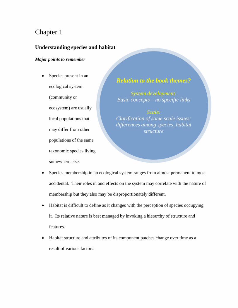
A community may comprise species entirely living in it, present because they are

present in the surrounding habitats, present only in portions of the community habitat, or

present in far away habitats that are also suitable but not connected to the habitat of interest

at the ecological time scale (although they may have been connected historically, Fig. 1.1).

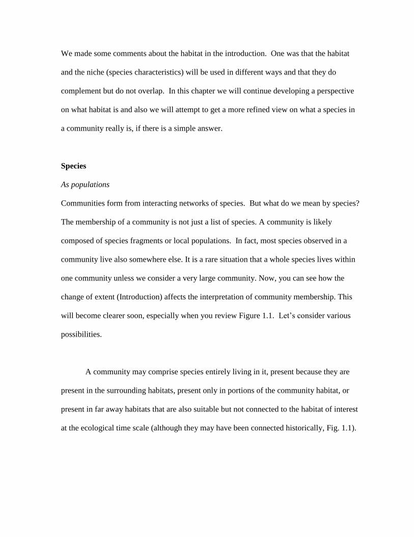
Fig. 2.1. A habitat such as an island in the

Okavango delta swamp (Botswana), marked in

red, is home to a community of organisms. Some

may belong to species whose population occupies

a single habitat of the island such as the sandy

beach (yellow species, Y), some may use all

habitats of whole island such as the red species,

R, and others, like the blue species, B, use many

other habitats, including the island ones. Note

that spatial relations among species are

asymmetric. Yellow species is within the ranges

of red and blue but blue is largely ‘free’ of the

presence of yellow and red and thus the potential

interactions between the three species will be

unequal in their mutual effects.

Fig. 1. 1. In a hypothetical community

Species A is abundant, but restricted to

relatively short occurrences over a

very limited space, which could be due

to habitat specialization and limited

immigration abilities. Species B is less

abundant but it shows persistence in

spite of being spatially restricted.

Thus, a local community is often a mixture of species to which the

local habitat is very important, species to which this habitat is optional or

occasional, and species that have any kind of intermediate relationship with

it. This applies to time dimension, too. Some species persist in a habitat

almost permanently, while others are mere transients. Also, some species are

represented by many while others by few individuals. The phase space

describing all the combinations along these dimensions can be filled in a variety of ways.

Figure 1.2 illustrates a couple of combinations as examples. Indeed, any single community

or ecosystem will have only some of this space filled and the way it is filled may depend on

history, kind of physical environment, and the scale of habitat of interest (particularly, its

extent).

Furthermore, the species observed in a community may show varying degrees of

integration with their own broader populations. How distinct locally they are depends on

whether individuals migrate into community or are born in it. The latter depends on habitat

isolation relative to species dispersal; poorly dispersed species are likely to rely more on

local reproduction than on immigration of individuals from outside. The

level of integration a local population has with the remaining populations of

the species matters because it determines to what degree the local population

depends on what happens in the local community. The less connected it is to

the outside, the more likely its interactions with other species in the local

community will determine its growth or demise. Those species whose local individuals are

most linked to the outside populations are transients: Individuals of some species, whether

How a local

population is

integrated with

‘sister’ populations

outside affects its

responses to other

community

members

‘Species’ in a

community or

ecosystem are

usually small local

populations of

species that have

much broader

geographical and

ecological

distribution

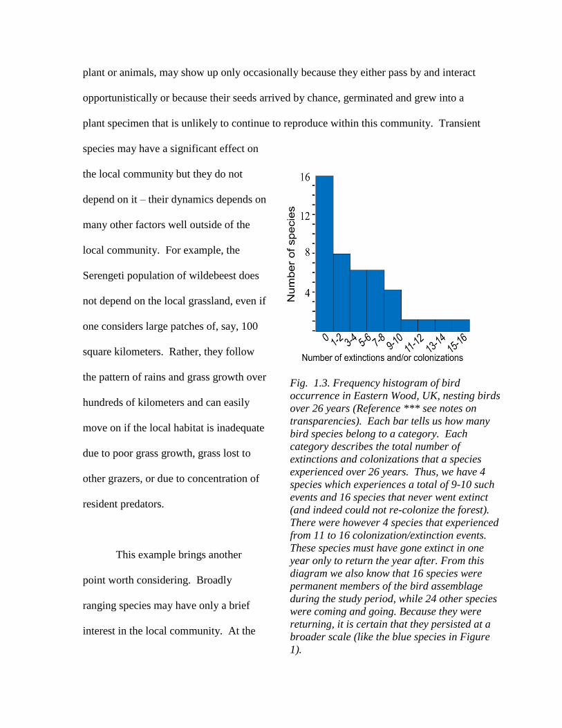
plant or animals, may show up only occasionally because they either pass by and interact

opportunistically or because their seeds arrived by chance, germinated and grew into a

plant specimen that is unlikely to continue to reproduce within this community. Transient

species may have a significant effect on

the local community but they do not

depend on it – their dynamics depends on

many other factors well outside of the

local community. For example, the

Serengeti population of wildebeest does

not depend on the local grassland, even if

one considers large patches of, say, 100

square kilometers. Rather, they follow

the pattern of rains and grass growth over

hundreds of kilometers and can easily

move on if the local habitat is inadequate

due to poor grass growth, grass lost to

other grazers, or due to concentration of

resident predators.

This example brings another

point worth considering. Broadly

ranging species may have only a brief

interest in the local community. At the

Fig. 1.3. Frequency histogram of bird

occurrence in Eastern Wood, UK, nesting birds

over 26 years (Reference *** see notes on

transparencies). Each bar tells us how many

bird species belong to a category. Each

category describes the total number of

extinctions and colonizations that a species

experienced over 26 years. Thus, we have 4

species which experiences a total of 9-10 such

events and 16 species that never went extinct

(and indeed could not re-colonize the forest).

There were however 4 species that experienced

from 11 to 16 colonization/extinction events.

These species must have gone extinct in one

year only to return the year after. From this

diagram we also know that 16 species were

permanent members of the bird assemblage

during the study period, while 24 other species

were coming and going. Because they were

returning, it is certain that they persisted at a

broader scale (like the blue species in Figure

1).

same time they are members of a much larger ecological system and thus their dynamics is

best understood at the scale of a larger system. A study of birds in a small forest patch in

Great Britain reveals some composition complexity typical of practically every ecological

system, whether small or large (Fig. 1.3).

Thus, we may think that each community is made up of species whose membership

ranges from obligatory (always present in the area delineating the community) to optional.

Species participate in community processes unequally with respect to their numbers, time

of ‘involvement’, and activities they engage in. The balance between the various classes of

members may change depending on the habitat/community type, its stage of development

(succession), and external influences such as pollution, destruction of surrounding habitat,

and many others.

Why is it important to remember that an ecological system is made up of

populations while we use species names to identify their general characteristics? An

example helps make the point. Troost et al. (2005) investigated adaptation of protists

living in under a gradient of light. In a homogeneous environment these

theoretical organisms are generalists because they use mixotrophy: they use

both photosynthesis and consumption of organic materials to satisfy their

energetic and nutritional needs. However, when presented with a gradient of

light availability, they specialize. Populations living where light is scarce

give up photosynthesis and switch to heterotrophy alone. Populations living in well lit

conditions specialize in autotrophic feeding via photosynthesis. The implication for

Populations of the

same species may

have widely

different

characteristics

depending on the

host habitat

community ecologists is that the same taxonomic species may in fact act as two or three

distinctly different ecological entities depending on the characteristics of habitat. What is

more, introducing spatial heterogeneity also makes evolution of these populations sensitive

to other environmental conditions, such as total nitrogen content or light intensity. As such,

it provides an explanation of why mixotrophs are often more dominant in nutrient-poor

systems while specialist strategies are associated with nutrient-rich systems (Troost et al.

2005).

This example and preceding considerations tell us that using the species name alone

does not give us a good sense of what traits this species has in ecological terms. More

information is required and remembering that actually it is the population that is a member

of community helps to keep this in better perspective.

Species traits

Not only species differ in when and for how long they are members of an ecological system

but they also do so in virtually any other characteristic. If the list of species is sufficiently

long, we will find clear gradients of other features. Species that differ in the number of

offspring they produce may form a reproductive strategy gradient (recall r- and K-

strategists). Species that differ in kinds of food, shelter, or microhabitat needed may form a

gradient of resource utilization. Autotrophic species that differ in biomass or rate of

growth may form a gradient of contributions to the energy budget of the local ecosystem.

Species that employ chemical defenses may form still another gradient of traits (by

chemical effectiveness or concentration). Or species restricted by various adverse or

unsuitable features of the habitat may form a gradient of habitat specialization. The

universality of this gradient is well illustrated by Dyer et al. (2007) who studied host

specificity of butterflies. Host specificity measures one of the dimensions that one could

include in species niche. They found that in every of eight locations they investigated from

Canada to Ecuador there were species that used five or less plant host genera as well as

some species that used more plant genera. Thus, they found that each butterfly assemblage

is a collection of species of different levels of specialization. In addition they found that

butterflies (their caterpillars) are progressively more specialized in the tropics.

Yet, while the above picture indicates some fluidity to which species make up a

community, some constraints apply. The community membership may appear haphazard

but local habitat attributes impose soft rules on which species can participate in communal

living and how they do so.

Niche as an ecological characteristic of a species

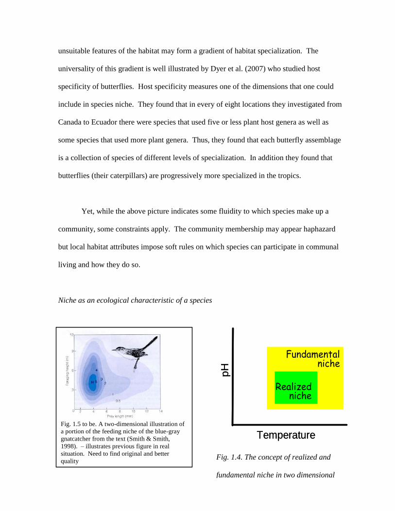
Fig. 1.4. The concept of realized and

fundamental niche in two dimensional

space.

Fig. 1.5 to be. A two-dimensional illustration of

a portion of the feeding niche of the blue-gray

gnatcatcher from the text (Smith & Smith,

1998). – illustrates previous figure in real

situation. Need to find original and better

quality

Temperature

pH

Temperature

pH

Fundamental niche

Realized niche

So far we recognized that species differ

in their traits how this is important to

understanding makeup of communities. These

differences and some of their consequences

have been examined by ecologists by

employing a concept of ecological niche.

Several approaches exist to characterization

and quantification of species traits but among

those the niche breadth is the most common

and well developed. Other concepts, related

but also slightly different in their emphasis or

scope, are tolerance and ecological range.

Niche does not have a good definition but it

can be loosely summarized as a set of biotic

and abiotic dimensions that describes

conditions a species can live under (or lives

under). Because it describes a species, niche is

analogous to some extent to morphology. This

view of the niche is due to E.G. Hutchinson

who first defined the niche as a species

characteristic. Usually, niche is portrayed using

one, two, or three dimensions, where values

suitable for a species become sides of a box.

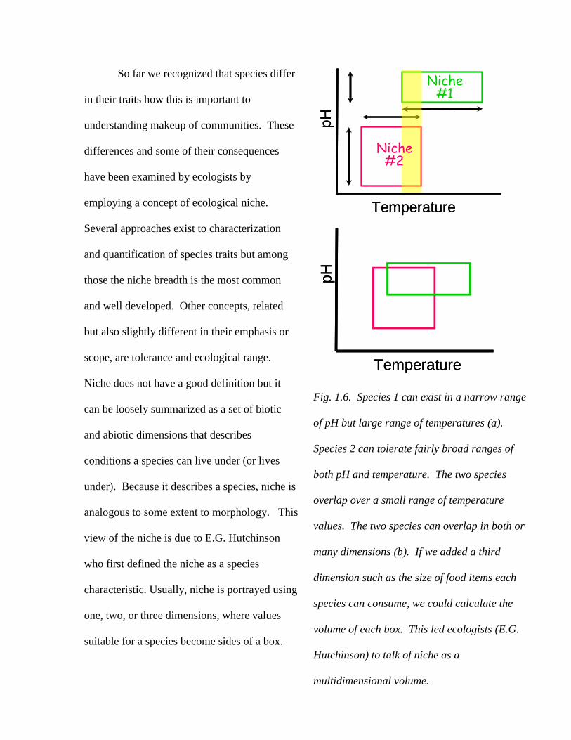
Fig. 1.6. Species 1 can exist in a narrow range

of pH but large range of temperatures (a).

Species 2 can tolerate fairly broad ranges of

both pH and temperature. The two species

overlap over a small range of temperature

values. The two species can overlap in both or

many dimensions (b). If we added a third

dimension such as the size of food items each

species can consume, we could calculate the

volume of each box. This led ecologists (E.G.

Hutchinson) to talk of niche as a

multidimensional volume.

Temperature

pH

Temperature

pH

Temperature

pH

Temperature

pH

Niche #2

Niche #1

Indeed, many dimensions are required for a more complete description of a species’ niche.

In two dimensions the box becomes a picture of the species’ niche.

Is mentioned earlier, ecologists used the niche concept to ask important questions

about species abundance and distribution, diversity-productivity relationship, community

stability, ecosystem functioning , and biological invasions . Current views highlight the

importance of the niche concept in ecology, and understanding different properties of

niches (e.g. use of environmental space, resource use) is also a key for understanding

community organisation (Chase and

Leibold, 2003).

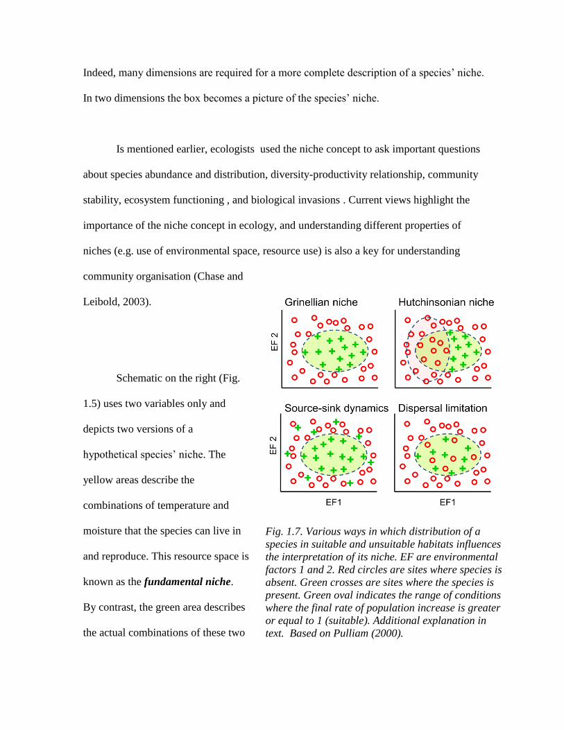
Schematic on the right (Fig.

1.5) uses two variables only and

depicts two versions of a

hypothetical species’ niche. The

yellow areas describe the

combinations of temperature and

moisture that the species can live in

and reproduce. This resource space is

known as the fundamental niche.

By contrast, the green area describes

the actual combinations of these two

Fig. 1.7. Various ways in which distribution of a

species in suitable and unsuitable habitats influences

the interpretation of its niche. EF are environmental

factors 1 and 2. Red circles are sites where species is

absent. Green crosses are sites where the species is

present. Green oval indicates the range of conditions

where the final rate of population increase is greater

or equal to 1 (suitable). Additional explanation in

text. Based on Pulliam (2000).

variables that the species utilizes in its habitat. This subset of the fundamental niche is

known as the realized niche. Fundamental niche represents species potential or capability

while the realized niche is often seen as being reduced by biotic factors such as competition

or predation. For example, leopards can and often do hunt during both the day and night.

However, in areas of high lion density, a species that strongly competes with leopards and

kills them whenever possible, leopards limit their hunting to the night. Thus their temporal

dimension for hunting is much smaller than their behavioral abilities permit. Furthermore,

a species may easily disperse to habitats that are suboptimal and that would not maintain

the population through the natural growth. Such habitats may appear as suitable if one

relied on the distribution of species alone. Some of the possible relations between species

niche, its distribution, and its habitat were reviewed by Pulliam (2000) and appear in Figure

1.7. Grinellian niche views species as being present in suitable habitat (final rate of

population increase equal or greater than 1). Hutchinsonian niche implies exclusion of

species from some sites due to biotic interactions – actual distribution is thus less than the

potential one. Source-sink dynamics permits species existence outside suitable patches

(final rate of increase less than 1). Dispersal limitation emphasizes the possibility that

species is absent from suitable sites because it is unable to disperse to them after they

formed or after species disappeared from them. The different processes captured by each

cartoon together underscore the difficulty of deducing niche properties from distribution

and habitat properties. They further underscore the need for clear separation of the three

concepts.

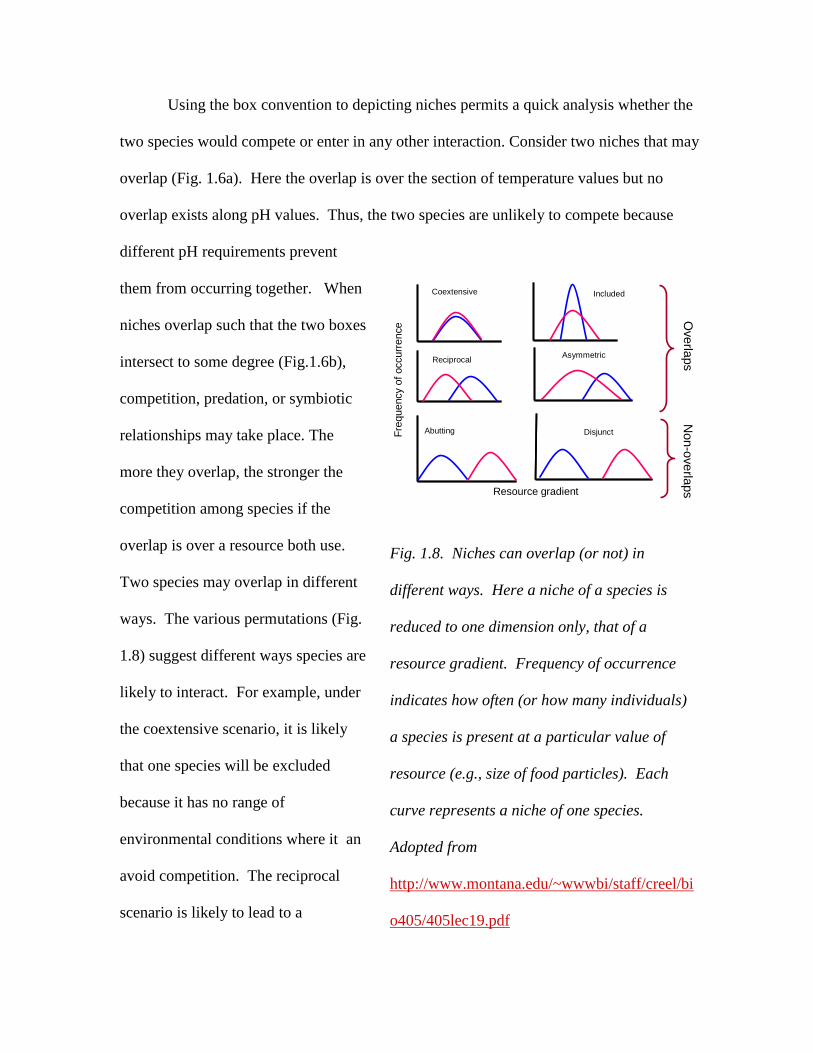
Using the box convention to depicting niches permits a quick analysis whether the

two species would compete or enter in any other interaction. Consider two niches that may

overlap (Fig. 1.6a). Here the overlap is over the section of temperature values but no

overlap exists along pH values. Thus, the two species are unlikely to compete because

different pH requirements prevent

them from occurring together. When

niches overlap such that the two boxes

intersect to some degree (Fig.1.6b),

competition, predation, or symbiotic

relationships may take place. The

more they overlap, the stronger the

competition among species if the

overlap is over a resource both use.

Two species may overlap in different

ways. The various permutations (Fig.

1.8) suggest different ways species are

likely to interact. For example, under

the coextensive scenario, it is likely

that one species will be excluded

because it has no range of

environmental conditions where it an

avoid competition. The reciprocal

scenario is likely to lead to a

Fig. 1.8. Niches can overlap (or not) in

different ways. Here a niche of a species is

reduced to one dimension only, that of a

resource gradient. Frequency of occurrence

indicates how often (or how many individuals)

a species is present at a particular value of

resource (e.g., size of food particles). Each

curve represents a niche of one species.

Adopted from

http://www.montana.edu/~wwwbi/staff/creel/bi

o405/405lec19.pdf

Overla

ps

Non-o

ve

rlaps

Fre

quency o

f occurr

ence

Resource gradient

Included

Reciprocal

Coextensive

Asymmetric

Abutting Disjunct

substantial reduction of realized niches but both species should be able to coexist by

selecting patches of habitat where they do not have to compete directly with the other

species. The asymmetric scenario gives more habitat to one of the species but the other can

still find a decent range of condition where to retreat. The case of lions and leopards would

fit here nicely. The non-overlapping situations are also of some interest because,

depending on whether the species abut or are disjunct (distinctly separated) on the resource

gradient, their potential for interaction is large or small if conditions slightly change. You

can try to think what outcomes would be likely under the remaining scenarios in Figure 1.8.

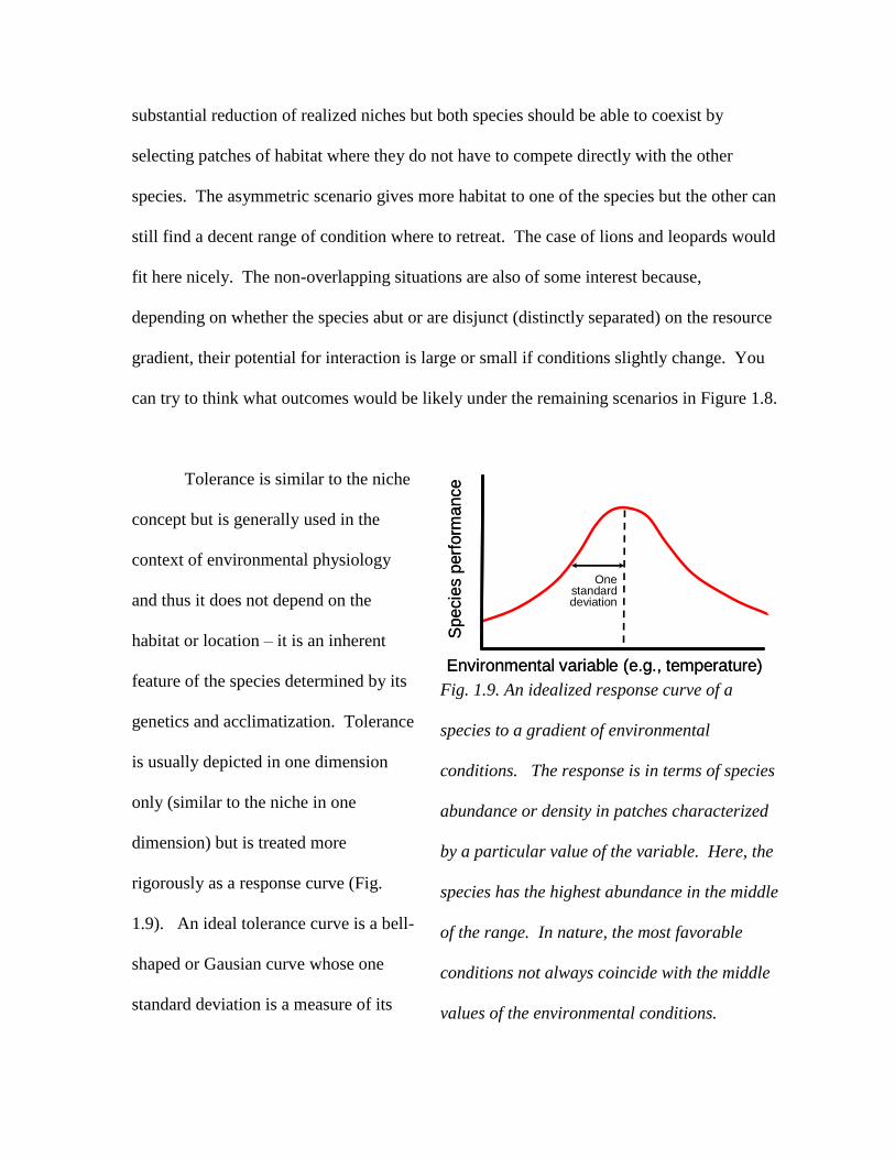
Tolerance is similar to the niche

concept but is generally used in the

context of environmental physiology

and thus it does not depend on the

habitat or location – it is an inherent

feature of the species determined by its

genetics and acclimatization. Tolerance

is usually depicted in one dimension

only (similar to the niche in one

dimension) but is treated more

rigorously as a response curve (Fig.

1.9). An ideal tolerance curve is a bell-

shaped or Gausian curve whose one

standard deviation is a measure of its

Fig. 1.9. An idealized response curve of a

species to a gradient of environmental

conditions. The response is in terms of species

abundance or density in patches characterized

by a particular value of the variable. Here, the

species has the highest abundance in the middle

of the range. In nature, the most favorable

conditions not always coincide with the middle

values of the environmental conditions.

Environmental variable (e.g., temperature)

Specie

s p

erf

orm

ance

Environmental variable (e.g., temperature)

Specie

s p

erf

orm

ance

One standard deviation

spread. The concept of the niche discussed above has been inspired by the tolerance curve

and it indistinguishable from it when a single variable/dimension is considered only. When

it comes to variables that do not affect physiology, the curve has a much lesser probability

of having bell shape. A response curve to predator is more likely to be monotonically

declining – it is not logical to expect that the species will improve its performance when its

predator density increases.

Ecological range is a related concept to that of the realized niche but it has some

additional flexibility. Which of the descriptors of species’ ability is used depends on the

question. For example, in a system of rock pools with differing environmental conditions

species can occur in some pools but cannot occur in others. However, species are often

absent from some of the pools whose conditions they can tolerate. The reason for such

absences is not therefore their tolerance (or niche parameters) but something else. A

species may fail to be present by chance when dispersing individuals simply missed the

opportunity; it may be absent due to history if it was pushed to extinction by past

perturbations and failed to return; and it can be absent because it is systematically or

occasionally reduced to zero numbers by competition, predation, or diseases. Neither

chance events nor history can be part of the niche volume because they would make a niche

volume not a characteristic of a species but a random value. However, the ecological range

is an effective measure of a species’ performance in a specified landscape – landscape of

rock pools in our example. Ecological range of a species may be different in a different

landscape. However, the effective (actual) ecological range in any specified landscape tell

us a lot about the species success and its ability to meet successfully other

species occupying the same space.

Habitat

What do we mean by habitat?

Habitat is rather difficult to define. A useful approach would be to ask what is habitat from

the user (a local population of a species) point of view. When you think of any two

species, even closely related species that occupy the same area, you will realize that they

use that area differently. Wolves and coyotes may share Yellowstone National Park but

hunt different prey, and coyotes keep their distance from wolves while wolves do no limit

their movement and hunting on account of coyotes. In Algonquin Provincial Park in

Ontario moose and white-tail deer live in the same area but use open spaces, lake shores

and swamps differently as well as show different levels of vulnerability to predators and

harsh winters. Thus, wolves and coyotes or moose and white-tail deer experience their

habitat differently. For all ecological purposes they live in somewhat different habitats

even though they occupy the same ecological system. Such differences in how coexisting

species see their habitat depend on the evolutionary distance between them as well as on

another, very important aspect of habitat structure (see further).

Ecological range

and the niche,

realized niche in

particular, are

related but not the

same

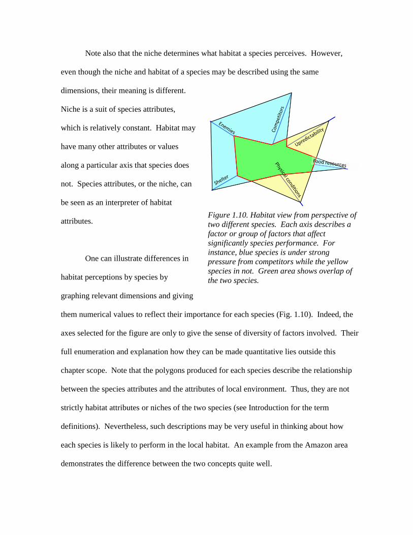
Note also that the niche determines what habitat a species perceives. However,

even though the niche and habitat of a species may be described using the same

dimensions, their meaning is different.

Niche is a suit of species attributes,

which is relatively constant. Habitat may

have many other attributes or values

along a particular axis that species does

not. Species attributes, or the niche, can

be seen as an interpreter of habitat

attributes.

One can illustrate differences in

habitat perceptions by species by

graphing relevant dimensions and giving

them numerical values to reflect their importance for each species (Fig. 1.10). Indeed, the

axes selected for the figure are only to give the sense of diversity of factors involved. Their

full enumeration and explanation how they can be made quantitative lies outside this

chapter scope. Note that the polygons produced for each species describe the relationship

between the species attributes and the attributes of local environment. Thus, they are not

strictly habitat attributes or niches of the two species (see Introduction for the term

definitions). Nevertheless, such descriptions may be very useful in thinking about how

each species is likely to perform in the local habitat. An example from the Amazon area

demonstrates the difference between the two concepts quite well.

Figure 1.10. Habitat view from perspective of

two different species. Each axis describes a

factor or group of factors that affect

significantly species performance. For

instance, blue species is under strong

pressure from competitors while the yellow

species in not. Green area shows overlap of

the two species.

Fine at al. (2004) wondered why they

observed distinct plant communities on two

different types of soil, sand and clay. They

transplanted seedlings of 20 species from six

genera of phylogenetically unrelated pairs of

edaphic (=soil) specialist trees. Trees growing

normally on clay soils were transplanted into

sandy soils and vice versa. They also

manipulated the presence of herbivores. They

found that clay specialist species grew

significantly faster than white-sand specialists

in both soil types when protected from

herbivores. However, when unprotected, white-sand specialists dominated in white-sand

forests and clay specialists dominated in clay forests. Fine and colleagues concluded that

habitat specialization in that system results from an interaction of herbivore pressure with

soil type. What is of interest to us here is that species abilities resulting from their

evolutionarily acquired traits (the niche) were obscured by contingent attributes of the

environment – not even one factor but an combination of two environmental axes (soil and

herbivores).

Box. 1.1. To consider… Where is the Figure 1.10 coming from? First, recall that the niche is an ecological characterization of species. It is usually thought of in terms of a variety of dimensions and species performance along those dimensions (Introduction). These dimensions may be exactly as those shown in Fig. 1.9 but may also include others that do not apply in the habitat we consider. For example, a species may have anti-predator defenses but when predators are absent, a comparison would make no sense. Thus, a value on an axis is produced by relating species traits to the state of the environment. If both species need shelter equally but the shelter is too small for the yellow, it will have a lower value on its axis.

Habitat structure

The differences in how species perceive

habitat and how they respond to it have

major systematic consequences. Species

occupying a local habitat differ not only in

response to specific habitat properties but

also in resolution of habitat grain (see

Introduction). However, the habitat grain

differences are not simply due to the fact

that some habitat components are large

while others are small. Rather they are due

to how those components are arranged

with respect to each other. But first …

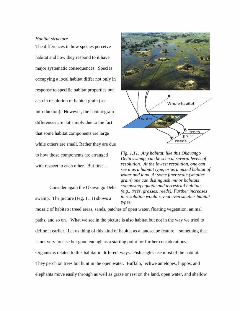
Consider again the Okavango Delta

swamp. The picture (Fig. 1.11) shows a

mosaic of habitats: treed areas, sands, patches of open water, floating vegetation, animal

paths, and so on. What we see in the picture is also habitat but not in the way we tried to

define it earlier. Let us thing of this kind of habitat as a landscape feature – something that

is not very precise but good enough as a starting point for further considerations.

Organisms related to this habitat in different ways. Fish eagles use most of the habitat.

They perch on trees but hunt in the open water. Buffalo, lechwe antelopes, hippos, and

elephants move easily through as well as graze or rest on the land, open water, and shallow

Fig. 1.11. Any habitat, like this Okavango

Delta swamp, can be seen at several levels of

resolution. At the lowest resolution, one can

see it as a habitat type, or as a mixed habitat of

water and land. At some finer scale (smaller

grain) one can distinguish minor habitats

composing aquatic and terrestrial habitats

(e.g., trees, grasses, reeds). Further increases

in resolution would reveal even smaller habitat

types.

reed and floating vegetation patches. However, monkeys are restricted to

dry areas while tiger fish is at home in open or quasi open water. From the

perspective of these organisms, habitat is actually a collection of more or

less suitable patches. Some organisms distinguish smaller, better defined kinds of habitat

than others. Thus, organisms living there see the swamp habitat as a mosaic of different

habitat types, which in turn are composed of mosaics of smaller habitat types, and so on.

An arrangement of things where larger

units contain smaller units is hierarchy (see

Introduction) – a condition of nestedness.

Of course, each single species may see

(use) only one type of habitat but as a

community they see the full richness of

habitat types.

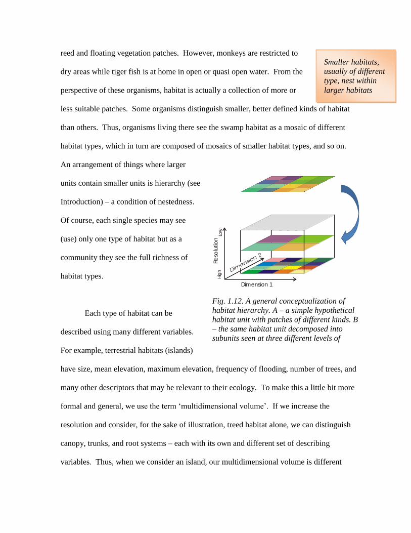
Each type of habitat can be

described using many different variables.

For example, terrestrial habitats (islands)

have size, mean elevation, maximum elevation, frequency of flooding, number of trees, and

many other descriptors that may be relevant to their ecology. To make this a little bit more

formal and general, we use the term ‘multidimensional volume’. If we increase the

resolution and consider, for the sake of illustration, treed habitat alone, we can distinguish

canopy, trunks, and root systems – each with its own and different set of describing

variables. Thus, when we consider an island, our multidimensional volume is different

Smaller habitats,

usually of different

type, nest within

larger habitats

Fig. 1.12. A general conceptualization of

habitat hierarchy. A – a simple hypothetical

habitat unit with patches of different kinds. B

– the same habitat unit decomposed into

subunits seen at three different levels of

resolution

Dimension 1

Re

solu

tion

Low

Hig

h

from that of a treed habitat, and so on. To capture this trend, we can start with a working

assumption that habitat is a nested hierarchy of multidimensional volumes (Fig. 1.12).

Because any dimension except time can be mapped onto space, we interpret the

habitat as a hierarchical mosaic of patches arranged such that lower level patches nest

within higher level patches, with this being true for each successive level of resolution.

Furthermore, each level and its patches may involve a distinct set of attributes. For

example, the top level in our Okavango swamp will be characterized by a ratio of water to

land. But each island (or water habitat) can be described using different variables (size,

elevation, plant cover, etc., but no longer by the ratio of water to land surface!) and each of

these habitats has its own descriptors that are appropriate. For the sake of graphical

illustration, we will use two dimensions only instead of the more realistic multidimensional

volume. This simplification gives the representation of habitat (or its model) a spatial

appearance even though this appearance represents a simplification. It does not purport to

convey any specific configuration of actual habitats in space. The model only identifies the

total amount of space a particular habitat unit occupies on average relative to a higher level

unit. Each unit can take various configurations in space as a patch that is either contiguous

or fragmented to varying degrees. Regardless of spatial configuration, each two distinct

and different habitat types are represented in the model as two subunits. Extending this

approach permits representation of the whole habitat as a nested structure of units emerging

at increasing levels of resolution (higher resolution reveals more detail – it reveals finer

habitat units).

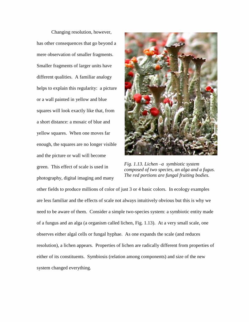
Changing resolution, however,

has other consequences that go beyond a

mere observation of smaller fragments.

Smaller fragments of larger units have

different qualities. A familiar analogy

helps to explain this regularity: a picture

or a wall painted in yellow and blue

squares will look exactly like that, from

a short distance: a mosaic of blue and

yellow squares. When one moves far

enough, the squares are no longer visible

and the picture or wall will become

green. This effect of scale is used in

photography, digital imaging and many

other fields to produce millions of color of just 3 or 4 basic colors. In ecology examples

are less familiar and the effects of scale not always intuitively obvious but this is why we

need to be aware of them. Consider a simple two-species system: a symbiotic entity made

of a fungus and an alga (a organism called lichen, Fig. 1.13). At a very small scale, one

observes either algal cells or fungal hyphae. As one expands the scale (and reduces

resolution), a lichen appears. Properties of lichen are radically different from properties of

either of its constituents. Symbiosis (relation among components) and size of the new

system changed everything.

Fig. 1.13. Lichen –a symbiotic system

composed of two species, an alga and a fugus.

The red portions are fungal fruiting bodies.

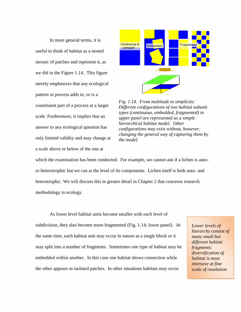
In more general terms, it is

useful to think of habitat as a nested

mosaic of patches and represent it, as

we did in the Figure 1.14. This figure

merely emphasizes that any ecological

pattern or process adds to, or is a

constituent part of a process at a larger

scale. Furthermore, it implies that an

answer to any ecological question has

only limited validity and may change at

a scale above or below of the one at

which the examination has been conducted. For example, we cannot ask if a lichen is auto-

or heterotrophic but we can at the level of its components. Lichen itself is both auto- and

heterotrophic. We will discuss this in greater detail in Chapter 2 that concerns research

methodology in ecology.

As lower level habitat units become smaller with each level of

subdivision, they also become more fragmented (Fig. 1.14; lower panel). At

the same time, each habitat unit may occur in nature as a single block or it

may split into a number of fragments. Sometimes one type of habitat may be

embedded within another. In this case one habitat shows connection while

the other appears as isolated patches. In other situations habitats may occur

Fig. 1.14. From multitude to simplicity:

Different configurations of two habitat subunit

types (continuous, embedded, fragmented) in

upper panel are represented as a simple

hierarchical habitat model. Other

configurations may exist without, however,

changing the general way of capturing them by

the model.

Lower levels of

hierarchy consist of

many small but

different habitat

fragments:

diversification of

habitat is most

intensive at fine

scale of resolution

as isolated patches neighboring similar or different patch types (Fig. 1.14; two left panels).

Furthermore, patches may be of different sizes and, indeed, the sizes of individual patches

rarely resemble one another in shape and size. Irrespective of the number of fragments into

each conceptual unit is split on the ground, the model remains the same (as shown in the

figure on the Figure 1.14; lower panel) where all four configurations of patches lead to the

same representation of the habitat structure.

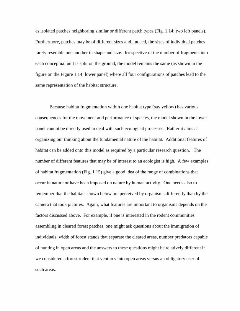
Because habitat fragmentation within one habitat type (say yellow) has various

consequences for the movement and performance of species, the model shown in the lower

panel cannot be directly used to deal with such ecological processes. Rather it aims at

organizing our thinking about the fundamental nature of the habitat. Additional features of

habitat can be added onto this model as required by a particular research question. The

number of different features that may be of interest to an ecologist is high. A few examples

of habitat fragmentation (Fig. 1.15) give a good idea of the range of combinations that

occur in nature or have been imposed on nature by human activity. One needs also to

remember that the habitats shown below are perceived by organisms differently than by the

camera that took pictures. Again, what features are important to organisms depends on the

factors discussed above. For example, if one is interested in the rodent communities

assembling in cleared forest patches, one might ask questions about the immigration of

individuals, width of forest stands that separate the cleared areas, number predators capable

of hunting in open areas and the answers to these questions might be relatively different if

we considered a forest rodent that ventures into open areas versus an obligatory user of

such areas.

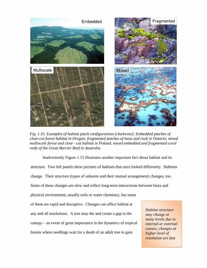
Inadvertently Figure 1.15 illustrates another important fact about habitat and its

structure. Two left panels show pictures of habitats that once looked differently. Habitats

change. Their structure (types of subunits and their mutual arrangement) changes, too.

Some of these changes are slow and reflect long-term interactions between biota and

physical environment, usually soils or water chemistry, but some

of them are rapid and disruptive. Changes can affect habitat at

any and all resolutions. A tree may die and create a gap in the

canopy – an event of great importance in the dynamics of tropical

forests where seedlings wait for a death of an adult tree to gain

Habitat structure

may change at

many levels due to

internal or external

causes; changes at

higher level of

resolution are fast

Fig. 1.15. Examples of habitat patch configurations (clockwise): Embedded patches of

clear-cut forest habitat in Oregon; fragmented patches of moss and rock in Ontario; mixed

multiscale forest and clear –cut habitat in Poland; mixed embedded and fragmented coral

reefs of the Great Barrier Reef in Australia.

light. At a forests stand level, changes are slow but at the individual herb or tree level

changes are much more frequent due to grazing, trampling, or seasonal life cycle. Structure

of the forest stand however may persist for longer periods of time. The causes of change

may both be internal (a tree fell as a result of its size and trunk or root system weakened by

parasites or weight added by vines and epiphytes) or it may be external (a strong wind or

lightning or soil erosion by the nearby stream). Internal causes of change as well as

external are very likely to differ depending on the scale of habitat under consideration. We

will look at some of these aspects, particularly at the links between spatial scale and

temporal scale of processes in the next chapter.

Self-test questions

1. Which portions of the phase space in Figure 1 would be likely to fill with

species if the figure pertained to a highly variable, unpredictable habitat?

How it would differ if the habitat was very stable and highly diversified into

smaller patches of distinct qualities to which species could specialize?

2. A sandy beach of an island is at a higher or lower level of habitat hierarchy

with respect to the island itself? Is it at a higher or lower level of resolution

with respect to the same island?

3. How many different habitat types can you think of when looking at each

picture in Figure 1.8? Try to write down all the possibilities …

Suggested readings

Wu 1999. ***