Embed Size (px)
Citation preview

THE HONG KONG POLYTECHNIC UNIVERSITY
DEPARTMENT OF ELECTRICAL ENGINEERING
Project ID: FYP_94
Communication Techniques for Autonomous(self-driving)
Vehicle Systems
by
TSE Yip Ming
14068068D
Final Report
Bachelor of Engineering (Honours)
in
Transportation Systems Engineering
Of
The Hong Kong Polytechnic University
Supervisor: Dr Alan P.T. Lau Date: 28 March 2018

THE HONG KONG POLYTECHNIC UNIVERSITY
DEPARTMENT OF ELECTRICAL ENGINEERING
Abstract
Wireless technology has been part and parcel of everyone’s life. Nonetheless, on top of
applying such a technology on the small gadgets, autonomous vehicle system for self-
driving can benefit from Wi-Fi communication to be more technologically mature.
Researchers have adopted various technique to develop this industry, yet not solve the
particular issue on autonomous vehicle system, especially on moving vehicles. The
distance value between vehicle and nearby roadside router determines the quality of
data transmission (described inversely by the Bit Error Rate) which depends on
different types of modulation (a process to transmit the signal through a communication
channel effectively by changing the properties of its own). Therefore, the proposed
method is to maximize transmission speed in an autonomous vehicle communication
by exploiting different types of modulations corresponding to the various distance
between transmitting end and receiving end. A systematic series of tasks with MATLAB
are used to demonstrate the feasibility of the method. For both Rayleigh Fading Model
and Rician Fading Model, the proposed method is found to outperform the traditional
method of using one type of modulation only in case of the received total bit at receiver
end against different vehicle speeds. After the recognition of the performance of the
proposed method, it is then put into practice by adopting adjustments for the purpose
of designing a well-rounded vehicle communication system through a new time-
division multiple access method such that every vehicle receives the same amount of
data. The result of simulation of applying the design vehicle communication system in
a more realistic road environment reflects that the design system is appropriate to be
utilized in reality. The optimal antenna distance obtained in the simulation provided the
best indication for placing the antenna, reducing the social cost of and time required for
numerous trials of various distances in practice.

THE HONG KONG POLYTECHNIC UNIVERSITY
DEPARTMENT OF ELECTRICAL ENGINEERING
Contents
1 Introduction ....................................................................................................................... 1
1.1 Objectives ................................................................................................................. 3
2 Literature Review .............................................................................................................. 4
3 Technical Skills and Methodology ..................................................................................... 6
3.1 The general process of WIFI communication .......................................................... 6
3.2 Noise Signal and Additive White Gaussian Noise (AWGN) ...................................... 8
3.3 Modulation ............................................................................................................. 10
3.3 Quadrature Amplitude Modulation (QAM) ........................................................... 11
3.4 Constellation diagrams for QAM............................................................................ 13
3.5 The wireless channel and Fading Model ................................................................ 15
3.6 Path Loss ................................................................................................................ 16
3.7 Shadowing .............................................................................................................. 18
3.8 Multipath ............................................................................................................... 19
3.9 Fading .................................................................................................................... 20
3.10 Fading Model ........................................................................................................ 22
3.11 Multiplexing and Multiple Access ......................................................................... 24
4 Progress and Simulation Results ..................................................................................... 28
4.1 BER against SNR for 4-QAM, 16-QAM and 64-QAM .............................................. 28
4.2 BER against SNR for 4-QAM, 16-QAM and 64-QAM with Fading Model ............... 29
4.3 Simulation of A Roadside Antenna Environment................................................... 31
4.4 The Proposed Method in multiple car situation .................................................... 41
4.5 The Proposed Method in multiple car situation with many antennas .................. 45
5 Conclusion and Future Development .............................................................................. 48
5.1 Conclusion .............................................................................................................. 48
5.2 Limitation ............................................................................................................... 49
5.3 Future Development .............................................................................................. 49
6 References ....................................................................................................................... 50

THE HONG KONG POLYTECHNIC UNIVERSITY
DEPARTMENT OF ELECTRICAL ENGINEERING
7 Appendix .......................................................................................................................... 52
7.1.1 Generation of BER against SNR for 4-QAM, 16-QAM, 64-QAM ............................. 52
7.1.2 Plot BER against SNR for 4-QAM, 16-QAM, 64-QAM ............................................. 54
7.2.1 Generation of BER against SNR for 4-QAM, 16-QAM, 64-QAM (Fading Model) ... 55
7.2.2 Plot BER against SNR for 4-QAM, 16-QAM, 64-QAM ( Fading Model ) ................. 58
7.3.1 Distance Function................................................................................................... 58
7.3.2 SNR dB Function ..................................................................................................... 58
7.3.3 BER Function .......................................................................................................... 59
7.3.4 QAM Order Function .............................................................................................. 61
7.3.5 Bits Rate Function .................................................................................................. 62
7.3.6 Total Bits Function ................................................................................................. 62
7.3.7 Plot Total Bits against Speed Function ................................................................... 63
7.3.8 Plot ALL Type Total Bits against Speed Function ................................................... 64
7.4.1 Create Car Start Point Function ............................................................................. 65
7.4.2 Distance km/hr to m/s unit Function ..................................................................... 65
7.4.2 Check Car QAM Order Function ............................................................................. 66
7.4.3 Traditional Time Division Method Function .......................................................... 67
7.4.4 Designed Time Division Method Function ............................................................. 67
7.4.5 Plot Traditional against Designed Time Division Method Function ....................... 68
7.5.1 Advanced Car QAM Order with Many Antennas Function .................................... 72
7.5.2 Travel with Many Antennas Function .................................................................... 75
7.5.3 Optimal Antenna Distance Function ...................................................................... 77
7.5.4 Plot Optimal Antenna Distance against Speed Function ....................................... 78

THE HONG KONG POLYTECHNIC UNIVERSITY
DEPARTMENT OF ELECTRICAL ENGINEERING
1
1 Introduction
With wireless technology developing in leaps and bounds, there is no one but utilizes
Wi-Fi on his or her smartphone to directly connect to the internet, so that everyone can
readily enjoy watching videos, playing games, and the list goes on. Nonetheless, never
should the pace of such a state-of-the-art technology stops on the small gadgets. In fact,
wireless communication is capable of being applied to a larger field – autonomous(self-
driving) vehicle systems. Notwithstanding the benefits, viz. improved road safety,
diminished emissions and enhanced mobility [1], brought by autonomous vehicle
systems, self-driving is technologically viable yet not sufficiently mature to be
prevalent.
Attracted by the advantage of autonomous vehicle system, scholars have adopted
different approaches such as applying training signal, coding technique and high-order
modulation to increase the performance of data transmission. There is no doubt that
their effort has a large contribution to the development of wireless communication, but
the problem of dealing with a particular area especially on self-driving system, the
moving vehicles issue, is still not solved. The distance value between vehicle and
vehicle or nearby roadside router is, in fact, an important factor to the quality of data
transmission which is described inversely by the Bit Error Rate (BER). At the same
time, the quality of data transmission in terms of the data rate also depends on different
types of modulation which are a process to transmit the signal through a communication
channel effectively by changing the properties of its own [2].
Maximization of the transmission speed of wireless communication in autonomous
vehicle network to the fullest is one of the possible approaches contributing to the

THE HONG KONG POLYTECHNIC UNIVERSITY
DEPARTMENT OF ELECTRICAL ENGINEERING
2
advancement in self-driving technology, which can be achieved by taking advantage of
different types of modulations corresponding to the various car-to-roadsides distance.
In signal processing, there exist modulation types from low-order to high-order in order
to transmit the signal effectively. A high-order modulation provides a high data rate
only at a short distance, but it lifts the Bit Error Rate at a long distance, while a low-
order modulation is capable maintaining a low Bit Error Rate in long-distance
communication, yet it is restricted by a low data rate.
Under the circumstance that vehicles are moving on a road, if the contemporary fixed
modulation is applied, either the data rate will be low, or Bit Error Rate will be high,
resulting in poor wireless communication. Hence, the proposed method is to harness
different modulations corresponding to various car-to-roadsides distances.
The proposed idea is achieved by a systematic series of tasks. MATLAB is used in
simulating vehicle communications. Rayleigh Fading Model and Rician Fading Model
are applied to imitate the authentic road environment. Several simulations are carried
out to figure out the different modulations at various Bit Error Rates to distances, to
design an optimal system to maximise the transmission speed in autonomous vehicle
network, and finally to compare the proposed method with the conventional method.

THE HONG KONG POLYTECHNIC UNIVERSITY
DEPARTMENT OF ELECTRICAL ENGINEERING
3
1.1 Objectives
1. To analyze the bit error rate against the distance between vehicles in different
modulation types.
2. To introduce the concept of correlation between Bit Error Rate in different
modulation types respect to various car-to-roadsides distance.
3. Use MATLAB stimulation to demonstrate the concept experiments and to compare
the proposed method with the conventional method.
4. Design an optimal system to maximize the transmission speed in autonomous
vehicle network by finding the optimal antenna distance for different vehicular
speed
THE HONG KONG POLYTECHNIC UNIVERSITY
DEPARTMENT OF ELECTRICAL ENGINEERING
4
2 Literature Review
The data transmission rate is high at a low-level Bit Error Rate in multiple-antenna
wireless communication. Hassibi and Hochwald [3] investigated the method of
adjusting the amount of training symbol to increase the data transferred. In general,
well-defined training signals are required to learn the knowledge of channel by sending
it from transmitter antenna to receiver antenna in some fraction of the transmission
period. This process is called training which has an influence on the capacity of the
fading channel. If training is not enough, the knowledge of the channel cannot be
obtained. If the training is excessive, the result will be an insufficient time for data
transmission before switching to the next channel. Therefore, the amount of training
symbol determines the data rate. In their study, there is an investigation into the
relationship between the amount of training and the number of transmit antenna. From
the experiment which is based on a satisfactory minimum requirement on the amount
of training for obtaining the capacity of the channel, the research team found that the
optimal solution is that the required number of training symbols should be the same as
the number of antennas, such that the training time in the transmission period is at a
minimum.
Currently, the bandwidth for wireless communication is limited which makes it difficult
to achieve a speedy data transmit. Tarokh et al. [4] adopted an approach which deals
with the physical layer through coding for improving the data transmission. They used
a multiple transmit antennas model and a space-time code to demonstrate their idea.
The complexity of the coding is similar to the trellis codes in the Gaussian channels.
The encoded data is divided into n streams and transmitted by n number of antennas at

THE HONG KONG POLYTECHNIC UNIVERSITY
DEPARTMENT OF ELECTRICAL ENGINEERING
5
the same time; then it is received by the receiver in terms of a superposition of n divided
streams with the additive noise. A delay diversity scheme is proposed to perform a copy
of the transmit signal which is less suffered from attenuation. In this scheme, the signal
is transmitted from multiple antennas but with a delay of one symbol rate. This method
ensures a high-quality signal in wireless communication without increasing the
bandwidth. In the modulation of 4-PSK and 8-PSK, this coding in their research has a
good performance with a low-level outage when using 2 bits per symbol with 64 state
encoders.
Another possible way to enhance the data transmission is adopting a high-order
modulation technique with a specified error-correcting code in WIFI communication.
This method can increase the amount of data transmitted per second. In general, a high-
order modulation 16-PSK is better than low-order modulation 4-PSK which is proposed
in [5]. However, the tradeoff increases the power input for the same Bit Error Rate. As
a result, a coding is required to deal with the power efficiency problem, but at the same
time, it increases the bandwidth by adding these codes into a transmitted symbol
sequence, lowering the bandwidth efficiency. In this situation, the research team
suggests increasing coded symbols for the redundancy of their proposed error-
correcting coding process. This code could be used to improve the power efficiency in
the AWGN channel without increasing the bandwidth. They have carried out several
experiments on the high-order modulation with this coding, 16-PSK, 16-QAM, and a
16-APK, under a limited band channel. The study pointed out that 16-PSK has an
excellent performance in data transmission. The 16-PSK modulation requires 5dB less
in signal to noise ratio than the 8-PSK modulation at the same symbol rate.

THE HONG KONG POLYTECHNIC UNIVERSITY
DEPARTMENT OF ELECTRICAL ENGINEERING
6
3 Technical Skills and Methodology
Few necessary relevant theories and terminologies are introduced here to illustrate the
proposed vehicle communication technique in the next chapter.
3.1 The general process of WIFI communication
A WIFI communication consists of several processes which include coding, modulation,
demodulation and decoding as illustrated in [6, Fig.1]. In this report, the focus only lies
on modulation, so it will be discussed in the later part.
In general, the information source is transmitted from the transmitter to the receiver,
and then the information is achieved in the destination such as computers in the vehicle.
The physical transmission medium which this signal passes through is called “channel”.
During this transmission, the noise will be introduced into the system as seen in [7,
Fig.2].
Figure 1 Flow Diagram of Information Processing.

THE HONG KONG POLYTECHNIC UNIVERSITY
DEPARTMENT OF ELECTRICAL ENGINEERING
7
Figure 2 General communications system.
For example, a sin wave source signal is to be transmitted from the transmitter to the
receiver in a communication system. The receiver end is supposed to receive a sin signal
identical to the source signal at the transmitter end as seen in [8, Fig.3], which is
represented by the dashed line. Under the introduction of noise in the communication
system, the received signal will mix up the source signal and the noise which distributes
the signal from the original, which is represented by the solid line. As a result, if the
amount of noise is too large, the source signal will be greatly affected, and it is difficult
for the receiver end to figure out if it is receiving a sin wave signal.
Figure 3 Received Signal with different amount of noise.
THE HONG KONG POLYTECHNIC UNIVERSITY
DEPARTMENT OF ELECTRICAL ENGINEERING
8
3.2 Noise Signal and Additive White Gaussian Noise (AWGN)
Noise is an unwanted signal that will cause interference with the source signal, and yet
it is usually unavoidable in the communication system [8]. There are a variety of noise
sources ranging from the external sources of the system to the internal sources of it, for
example, atmospheric noise caused by natural atmospheric processes and thermal noise
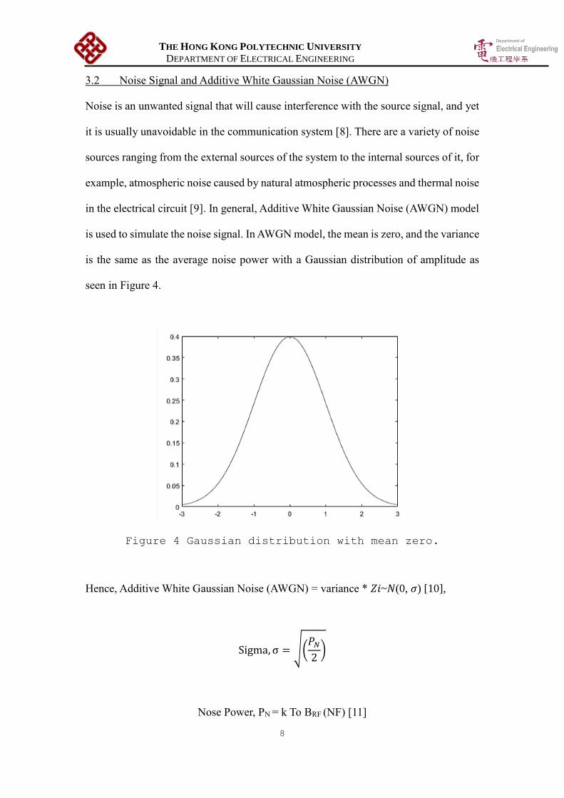
in the electrical circuit [9]. In general, Additive White Gaussian Noise (AWGN) model
is used to simulate the noise signal. In AWGN model, the mean is zero, and the variance
is the same as the average noise power with a Gaussian distribution of amplitude as
seen in Figure 4.
Figure 4 Gaussian distribution with mean zero.
Hence, Additive White Gaussian Noise (AWGN) = variance * 𝑍𝑖~𝑁(0, 𝜎) [10],
Sigma, σ = √(𝑃𝑁
2)
Nose Power, PN = k To BRF (NF) [11]

THE HONG KONG POLYTECHNIC UNIVERSITY
DEPARTMENT OF ELECTRICAL ENGINEERING
9
Symbol Notation
k Boltzmann Constant
To Temperature in Kelvin
BRF Bandwidth
NF Noise Figure
This property helps to simulate the effect of the “random process” of noise in nature.
In general, Signal-to-Noise Ratio SNR which is the ratio of Signal Power to the Noise
Power is used to express the quality of signal [11]. The higher the SNR value, the higher
quality of signal will be
SNR =𝑃𝑆
𝑃𝑁
Where 𝑃𝑇𝑋 refers to Signal Power. In general, SNR is always measured in dB unit.
Therefore, the formulas are
SNR (dB) = 10 log SNR
Sigma = √(𝑃𝑇𝑋
2 ∗ SNR)
Sigma = √(𝑃𝑇𝑋
2 ∗ 10𝑆𝑁𝑅𝑑𝐵
10
)
THE HONG KONG POLYTECHNIC UNIVERSITY
DEPARTMENT OF ELECTRICAL ENGINEERING
10
3.3 Modulation
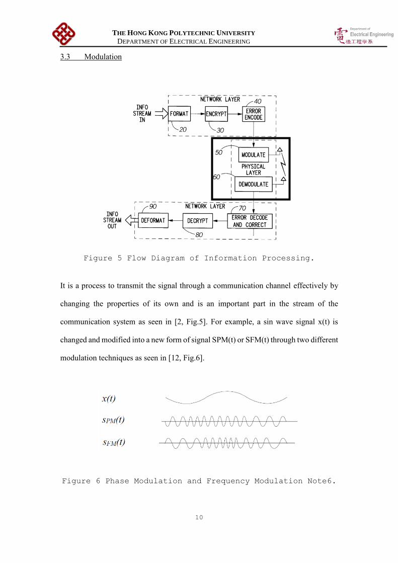
Figure 5 Flow Diagram of Information Processing.
It is a process to transmit the signal through a communication channel effectively by
changing the properties of its own and is an important part in the stream of the
communication system as seen in [2, Fig.5]. For example, a sin wave signal x(t) is
changed and modified into a new form of signal SPM(t) or SFM(t) through two different
modulation techniques as seen in [12, Fig.6].
Figure 6 Phase Modulation and Frequency Modulation Note6.

THE HONG KONG POLYTECHNIC UNIVERSITY
DEPARTMENT OF ELECTRICAL ENGINEERING
11
There are three types of fundamental digital modulation method which are Amplitude-
Shift Keying (ASK), Frequency-Shift Keying (FSK), and Phase-Shift Keying (PSK),
as well as a complex modulation type so-called Quadrature Amplitude Modulation
(QAM) [10].
In this project, the modulation type QAM will be focused. The idea of this project is
how to take advantage of the different type of QAM, 4-QAM, 16QAM and 64QAM, in
order to maximise the transmission speed.
3.3 Quadrature Amplitude Modulation (QAM)
Quadrature Amplitude Modulation (QAM) is a process of transmitting two Double
Sideband (DSB) signal as illustrated in [2, Fig.7] with same frequency simultaneously.
Figure 7 Double Sideband Signal.
One of the signals will have a phase different by 90 degrees to the other, thus achieving
the name Quadrature Modulation. Therefore, if m1(t) and m2(t) are the original signals,
then they will become m1(t)cos(Wct) and m2(t)sin(Wct) respectively while the
trigonometric function serves as a carrier with carrier frequency Wc to carry those
signals.

THE HONG KONG POLYTECHNIC UNIVERSITY
DEPARTMENT OF ELECTRICAL ENGINEERING
12
At the sending end, m1(t)cos(Wct) and m2(t)sin(Wct) will be added together to form
QAM(t) for sending [2]. Sending Signal:
QAM(t) = m1(t)cos(Wct)+m2(t)sin(Wct)
where m1(t) and m2(t) are the original signals
Figure 8 Quadrature Amplitude Modulation (QAM).
At the receiving end, the QAM signal will be demodulated by multiplying the term
2cos(Wct) and 2sin(Wct), that is
x1(t)= QAM(t) x 2cos(Wct) = m1(t) + m1(t) cos(2Wct) + m2(t)sin(2Wct)
x2(t)= QAM(t) x 2 sin(Wct) = m2(t) − m2(t) cos(2Wct) + m1(t)sin(2Wct)
Then, the signals are filtering by a suitable low-pass filter to remove the last two term
of x1(t) and x2(t). As a result, the receiver end could return the original signals m1(t)
and m2(t) as illustrated in [2, Fig.8].
THE HONG KONG POLYTECHNIC UNIVERSITY
DEPARTMENT OF ELECTRICAL ENGINEERING
13
3.4 Constellation diagrams for QAM
QAM(t) = m1(t) cos(Wct) + m2(t) sin(Wct) can also be written as
QAM(t) = R{ [ m1(t)- j m2(t) ] e jWct
} ,
hence s(t) = m1(t)- j m2(t) is obtained [10].
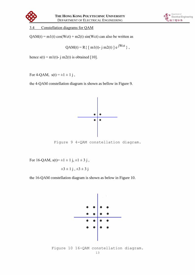
For 4-QAM, s(t) = ±1 ± 1 j ,
the 4-QAM constellation diagram is shown as bellow in Figure 9.
Figure 9 4-QAM constellation diagram.
For 16-QAM, s(t)= ±1 ± 1 j, ±1 ± 3 j ,
±3 ± 1 j , ±3 ± 3 j
the 16-QAM constellation diagram is shown as below in Figure 10.
Figure 10 16-QAM constellation diagram.

THE HONG KONG POLYTECHNIC UNIVERSITY
DEPARTMENT OF ELECTRICAL ENGINEERING
14
For 64-QAM, s(t)= ±1 ± 1 j, ±1 ± 3 j , ±1 ± 5 j , ±1 ± 7 j ,
±3 ± 1 j, ±3 ± 3 j , ±3 ± 5 j , ±3 ± 7 j ,
±5 ± 1 j, ±5 ± 3 j , ±5 ± 5 j , ±5 ± 7 j ,
±7 ± 1 j, ±7 ± 3 j , ±7 ± 5 j , ±7 ± 7 j
the 16-QAM constellation diagram is shown as below in Figure 11.
Figure 11 64-QAM constellation diagram.
As the purpose is to compare the efficiency of 4-QAM, 16-QAM and 64-QAM. The
transmitted power of all these types are same and are set as 1W. Therefore, s(t) should
be multiplied by a scaling factor for achieving N order of QAM in the condition of 1W
transmitted power. Let b be the Scaling Factor.
For 4-QAM,
(1b)2 × 2 × 1 × 4
4= 1W,
hence the Scaling Factor is 1
2 .

THE HONG KONG POLYTECHNIC UNIVERSITY
DEPARTMENT OF ELECTRICAL ENGINEERING
15
For 16-QAM,
[(1b)2 + (3b)2] × 2 × 2 × 4
16= 1W,
hence the Scaling Factor is 1
10 .
For 64-QAM,
[ (1b)2 + (3b)2 + (5b)2 + (7b)2] × 2 × 4 × 4
64= 1W,
hence the Scaling Factor is 1
42 .
3.5 The wireless channel and Fading Model
Wireless channel is the path of an electromagnetic wave through radiation process from
the transmitter antenna to the receiver antenna. The channel strength varies over time
and frequency as illustrated in [13, Fig.12].
Figure 12 Channel quality over time.
THE HONG KONG POLYTECHNIC UNIVERSITY
DEPARTMENT OF ELECTRICAL ENGINEERING
16
In general speaking, it can be determined by the distance and path between the
transmitter antenna and the receiver antenna. If the information of the wireless channel
is well-known, the figure of the received signal can be achieved. There are three
fundamental components to describe the characteristic of the wireless channel, path loss,
shadowing and multipath.
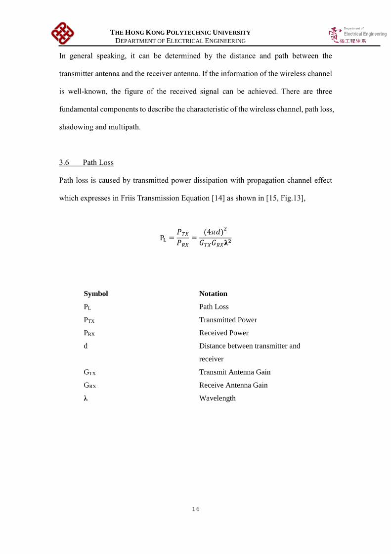
3.6 Path Loss
Path loss is caused by transmitted power dissipation with propagation channel effect
which expresses in Friis Transmission Equation [14] as shown in [15, Fig.13],
PL =𝑃𝑇𝑋
𝑃𝑅𝑋=
(4𝜋𝑑)2
𝐺𝑇𝑋𝐺𝑅𝑋𝛌𝟐
Symbol Notation
PL Path Loss
PTX Transmitted Power
PRX Received Power
d Distance between transmitter and
receiver
GTX Transmit Antenna Gain
GRX Receive Antenna Gain
λ Wavelength

THE HONG KONG POLYTECHNIC UNIVERSITY
DEPARTMENT OF ELECTRICAL ENGINEERING
17
Figure 13 Path Loss in a system.
In technical speaking, the received signal power decreases drastically with the
increase of the distance between the transmitter antenna and the receiver antenna.
With previous equation, path loss can be written as
PL =𝑃𝑇𝑋
𝑆𝑁𝑅 𝑅𝑋 ∙ 𝑃𝑁
=(4𝜋𝑑)2
𝐺𝑇𝑋𝐺𝑅𝑋𝛌𝟐
PL =𝑃𝑇𝑋
𝑆𝑁𝑅 𝑅𝑋 ∙ k ∙ To ∙ BRF ∙ (NF)=
(4𝜋𝑑)2
𝐺𝑇𝑋𝐺𝑅𝑋𝛌𝟐
PL =𝑃𝑇𝑋
𝑆𝑁𝑅 𝑇𝑋 ∙ k ∙ To ∙ BRF =
(4𝜋𝑑)2
𝐺𝑇𝑋𝐺𝑅𝑋𝛌𝟐
Therefore, SNR is proportional to 1
𝑑2 .
THE HONG KONG POLYTECHNIC UNIVERSITY
DEPARTMENT OF ELECTRICAL ENGINEERING
18
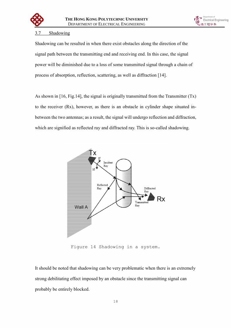
3.7 Shadowing
Shadowing can be resulted in when there exist obstacles along the direction of the
signal path between the transmitting end and receiving end. In this case, the signal
power will be diminished due to a loss of some transmitted signal through a chain of
process of absorption, reflection, scattering, as well as diffraction [14].
As shown in [16, Fig.14], the signal is originally transmitted from the Transmitter (Tx)
to the receiver (Rx), however, as there is an obstacle in cylinder shape situated in-
between the two antennas; as a result, the signal will undergo reflection and diffraction,
which are signified as reflected ray and diffracted ray. This is so-called shadowing.
Figure 14 Shadowing in a system.
It should be noted that shadowing can be very problematic when there is an extremely
strong debilitating effect imposed by an obstacle since the transmitting signal can
probably be entirely blocked.

THE HONG KONG POLYTECHNIC UNIVERSITY
DEPARTMENT OF ELECTRICAL ENGINEERING
19
In contrast with shadowing, variation of the signal strength in the wake of path loss
will usually occur in a very long distance, such as 100 to 1,000 metres. Instead,
variation that is resulted from shadowing will occur in a distance which is in
proportion with the length of the obstruction, which is usually 10 to 100 metres [14].
3.8 Multipath
Based on the aforementioned sections of path loss and shadowing, since it is
inevitable to get rid of the objects and obstacles on the road in reality; thus, there are
bound to be objects situated surrounding the path of signal between the transmitter
and receiver, such that the signal will be reflected ultimately. Consideration will be
taken only on the successfully received signal which is reflected to the receiver.
As the [14, Fig.15] demonstrates that every signal is taking a different path from one
and other; as a consequence, the amplitude and phase of reflected signals will be
ultimately different as well. It can be concluded that whether the summation of these
multiple reflected signal, as well as the direct path signal will result in an increased or
decreased received signal power is in fact dependent on the phase.
Figure 15 Multipath in a system.

THE HONG KONG POLYTECHNIC UNIVERSITY
DEPARTMENT OF ELECTRICAL ENGINEERING
20
It should be noted that any changes in the positions of the transmitter, receiver,
objects or obstacles, no matter how slight it is, can sufficiently give rise to a
considerable variation in received signal phases, thereby exerting impacts on the
received power as well.
3.9 Fading
Fading is generally referred to the recognizable impacts of changing received signal
strength over time. It is assumed that the result of these changes is initiated by the
variation in propagation effects from the transmitting end to the receiving end. It
should be noted that the result of these changes is not resulted from the variation in
the output power of transmitter [17].
The variation of channel strength due to the three fundamental components that are
mentioned above can be classified into two types: Large-scale fading and Small-scale
fading.
3.9.1 Large-scale fading
Large-scale fading is due to path loss caused by transmitted power dissipation with
propagation channel effect in large distance and shadowing caused by large obstacles
that absorbing, reflecting, scattering, and diffracting the transmitted power and is
usually frequency independent. The large-scale fading arises because of the
extraordinary influence on the received signal power imposed by the path loss and
shadowing as mentioned above [14].
THE HONG KONG POLYTECHNIC UNIVERSITY
DEPARTMENT OF ELECTRICAL ENGINEERING
21
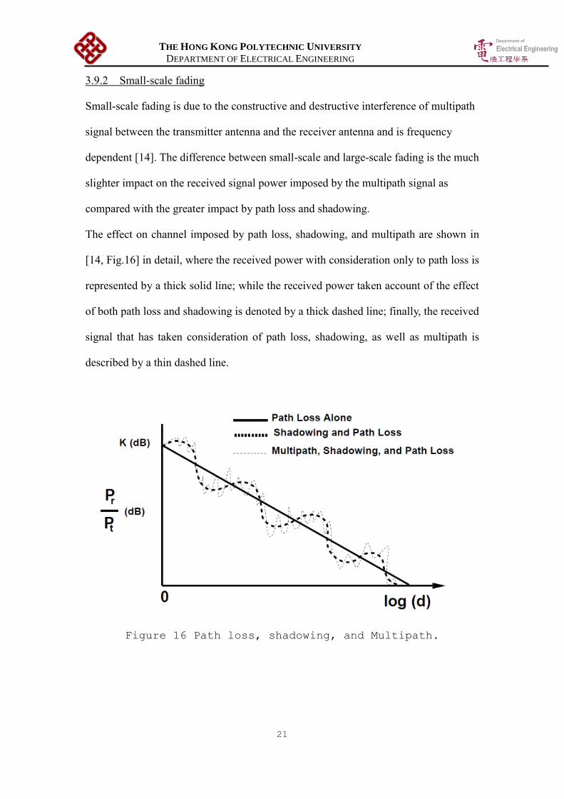
3.9.2 Small-scale fading
Small-scale fading is due to the constructive and destructive interference of multipath
signal between the transmitter antenna and the receiver antenna and is frequency
dependent [14]. The difference between small-scale and large-scale fading is the much
slighter impact on the received signal power imposed by the multipath signal as
compared with the greater impact by path loss and shadowing.
The effect on channel imposed by path loss, shadowing, and multipath are shown in
[14, Fig.16] in detail, where the received power with consideration only to path loss is
represented by a thick solid line; while the received power taken account of the effect
of both path loss and shadowing is denoted by a thick dashed line; finally, the received
signal that has taken consideration of path loss, shadowing, as well as multipath is
described by a thin dashed line.
Figure 16 Path loss, shadowing, and Multipath.

THE HONG KONG POLYTECHNIC UNIVERSITY
DEPARTMENT OF ELECTRICAL ENGINEERING
22
3.10 Fading Model
In general, Rician fading model and Rayleigh fading model are widely used to simulate
the wireless communication channel for which channel strength vary in an
unforeseeable way and can only be characterised statistically.
Rician fading model is used when there is a dominant Line-Of-Sight (LOS) path in
between the transmitter and the receiver as seen in [18, Fig.17]. In this situation, there
is a non-significant scattered field such that the reflected paths are weaker than the LOS
path. As a result, Rician fading mode is suitable for simulating an open area like rural
environment.
In contrast, Rayleigh fading model is used when there are large number paths scattered
by many small reflectors such that Line-Of-Sight (LOS) path is not dominant. In this
situation, there is a significant scattered field such that the reflected paths are stronger
than the LOS path. As a result, Rayleigh fading model is suitable for simulating an
urban area with a lot of buildings [13].
Figure 17 Multipath Propagation.

THE HONG KONG POLYTECHNIC UNIVERSITY
DEPARTMENT OF ELECTRICAL ENGINEERING
23
In rural environment, Rician fading model is applied and is expressed by following
equation
where KLOS is the ratio of energy in the LOS to those scattered paths, HLOS is a purely
deterministic matrix, and Hres has zero-mean Gaussian entries. If the distance between
transmitter and receiver is large, HLOS becomes one [19].
In urban environment, Rayleigh fading model is adopted and therefore KLOS is zero. It
is because there is no dominant Line-Of-Sight (LOS) path. Hence the first term of the
equation becomes zero, and the second term becomes Hres [13]. As a result, the
mathematic expression of Rayleigh fading model is
Considering the fading model, now the stimulation model’s equation becomes
𝒚[𝑚] = H ∙ 𝒙[𝑚] + 𝒘[𝑚]
where 𝒚[𝑚] is received power spectrum matrix, 𝒙[𝑚] is transmit power spectrum
matrix and 𝒘[𝑚] is AWGN spectrum matrix.
THE HONG KONG POLYTECHNIC UNIVERSITY
DEPARTMENT OF ELECTRICAL ENGINEERING
24
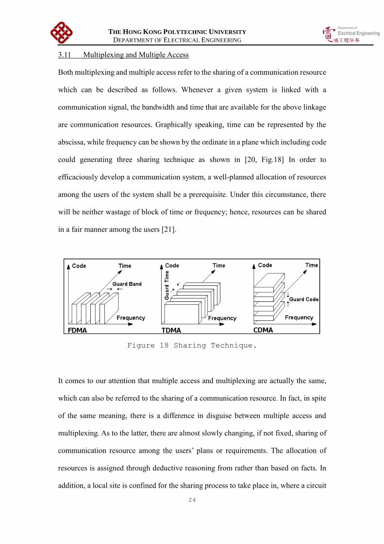
3.11 Multiplexing and Multiple Access
Both multiplexing and multiple access refer to the sharing of a communication resource
which can be described as follows. Whenever a given system is linked with a
communication signal, the bandwidth and time that are available for the above linkage
are communication resources. Graphically speaking, time can be represented by the
abscissa, while frequency can be shown by the ordinate in a plane which including code
could generating three sharing technique as shown in [20, Fig.18] In order to
efficaciously develop a communication system, a well-planned allocation of resources
among the users of the system shall be a prerequisite. Under this circumstance, there
will be neither wastage of block of time or frequency; hence, resources can be shared
in a fair manner among the users [21].
Figure 18 Sharing Technique.
It comes to our attention that multiple access and multiplexing are actually the same,
which can also be referred to the sharing of a communication resource. In fact, in spite
of the same meaning, there is a difference in disguise between multiple access and
multiplexing. As to the latter, there are almost slowly changing, if not fixed, sharing of
communication resource among the users’ plans or requirements. The allocation of
resources is assigned through deductive reasoning from rather than based on facts. In
addition, a local site is confined for the sharing process to take place in, where a circuit

THE HONG KONG POLYTECHNIC UNIVERSITY
DEPARTMENT OF ELECTRICAL ENGINEERING
25
board is a telling example. In contrast, with regard to multiple access, remote sharing
of the resource is very often involved. The remoteness can be as far as satellite
communications; as a result, the multiple access scheme is changing dynamically, in
which the needs of communication resource from each user had to be beware by a
system controller. In light of it, an overhead is given rise by the extra requirement of
the amount of time for such an information transfer, which in turn constitutes a
constraint on the efficiency of the utilization of communication resource, such that an
upper limit is required to be drawn [21].
Time Division Multiple Access
Time division multiple access is defined as multiplexing the division of time in
accordance with the number of channels set by oneself [22].
Figure 19 Schematic of T1 carrier system.
For example, according to the schematic of T1 carrier system as shown in [22, Fig.19],
time is division multiplexed with reference to 24 channels, while a TDM PAM signal
represents the sampler output. The Signal is firstly taken and then quantized by an
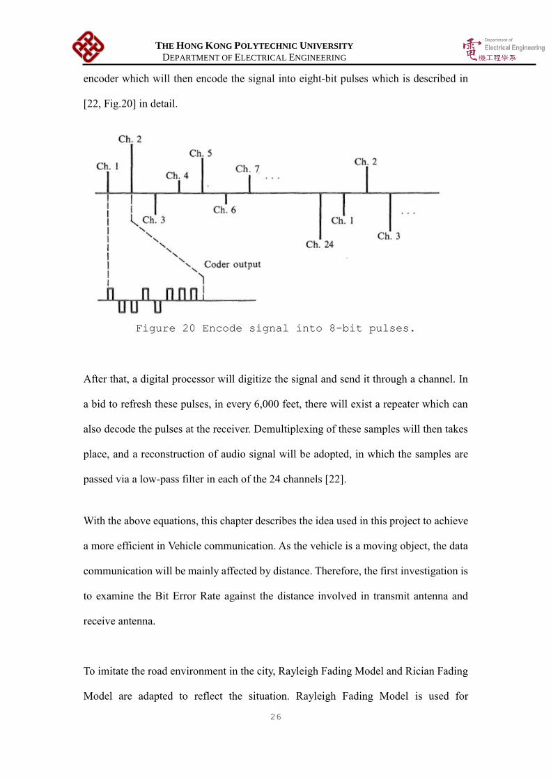
THE HONG KONG POLYTECHNIC UNIVERSITY
DEPARTMENT OF ELECTRICAL ENGINEERING
26
encoder which will then encode the signal into eight-bit pulses which is described in
[22, Fig.20] in detail.
Figure 20 Encode signal into 8-bit pulses.
After that, a digital processor will digitize the signal and send it through a channel. In
a bid to refresh these pulses, in every 6,000 feet, there will exist a repeater which can
also decode the pulses at the receiver. Demultiplexing of these samples will then takes
place, and a reconstruction of audio signal will be adopted, in which the samples are
passed via a low-pass filter in each of the 24 channels [22].
With the above equations, this chapter describes the idea used in this project to achieve
a more efficient in Vehicle communication. As the vehicle is a moving object, the data
communication will be mainly affected by distance. Therefore, the first investigation is
to examine the Bit Error Rate against the distance involved in transmit antenna and
receive antenna.
To imitate the road environment in the city, Rayleigh Fading Model and Rician Fading
Model are adapted to reflect the situation. Rayleigh Fading Model is used for

THE HONG KONG POLYTECHNIC UNIVERSITY
DEPARTMENT OF ELECTRICAL ENGINEERING
27
considering the non- Line-Of-Sight (LOS) environment which is suitable for urban area
with a lot of buildings and vehicles [23]. Autonomous vehicle network may not be
directly performed if there is a physical obstacle in between the transmitter on the
vehicle and receiver at the nearby roadside. For example, a car in between the
communication device. Therefore, this kind of non-direct connecting communication
can be regarded as under LOS environment. By contrast, Rician Fading Model can
represent and reflect the direct Line-Of-Sight communication which is suitable for rural
environment like the countryside road. [24].
MATLAB is used to simulate the road environment for wireless communication for
different level modulations from a low-order modulation such as 4-QAM to a high-
order modulation like 64-QAM. A graph of Bit Error Rate against Distance in various
modulation cases will be generated for analysis.
As expected in the concept idea, the low-order modulation should perform well in long
distance, but it allows only small bit rate for data transmission. The high-order
modulation performs well only in short distance, but it offers a high bit rate due to its
structure. A study is made to investigate the optimal range for each modulation and
hence design an optimal system for better data transmission.
Base on the idea, this optimal system is devised to maximise the transmission speed in
autonomous vehicle network by adopting a different level of modulation for various
distance. The criteria for switching the optimal modulation will refer to a factor of BER
limit, SNR value and distance between transmit antenna and receive antenna. When the
BER value exceeds the critical BER limit, high-order modulation will be changed to a
low-order modulation for better performance.

THE HONG KONG POLYTECHNIC UNIVERSITY
DEPARTMENT OF ELECTRICAL ENGINEERING
28
4 Progress and Simulation Results
The results are simulated by MATLAB, and the source code can be found at the
appendix page in the last chapter.
4.1 BER against SNR for 4-QAM, 16-QAM and 64-QAM
The simulation result of BER against SNR for 4-QAM, 16-QAM and 64-QAM is
shown in Figure 21.
Figure 21 BER against SNR simulation for 4-QAM, 16-QAM
and 64-QAM.
Due to the constellation structure, the low-order modulation 4-QAM performs well in
long distance as the BER is still in low value for small SNR. At the same time, the
high-order modulation 64-QAM performs well only in short distance as the BER
value is relatively high even for large SNR.

THE HONG KONG POLYTECHNIC UNIVERSITY
DEPARTMENT OF ELECTRICAL ENGINEERING
29
4.2 BER against SNR for 4-QAM, 16-QAM and 64-QAM with Fading Model
The project aims at simulating the performance of the proposed method by exploiting
different types of modulations corresponding to the distance between the transmitting
end and receiving end in the vehicle communication system. Therefore, using the result
from the previous simulation definitely does not suffice. Instead, it will be much better
to make the simulation more realistic by adopting the Rayleigh Fading Model and
Rician Fading Model. Rayleigh Fading Model and Rician Fading Model are best suit
the road environment, in which Rayleigh Fading Model represents the road
environment in urban area with no dominant Line-Of-Sight(LOS) path between two
antennas, whereas Rician Fading Model demonstrates the road environment in rural
area with dominant Line-Of-Sight(LOS) path.
For urban environment, Rayleigh Fading Model is simulated with KLOS =0, the BER
against SNR for 4-QAM, 16-QAM and 64-QAM is shown in Figure 22.
Figure 22 BER against SNR simulation in Rayleigh fading
for 4-QAM, 16-QAM and 64-QAM.

THE HONG KONG POLYTECHNIC UNIVERSITY
DEPARTMENT OF ELECTRICAL ENGINEERING
30
For rural environment, Rician Fading Model is simulated with KLOS dB=3dB [25],
hence KLOS =2. Hence, the simulation result of the BER against SNR for 4-QAM, 16-
QAM and 64-QAM is shown in Figure 23.
Figure 23 BER against SNR simulation in Rician fading for
4-QAM, 16-QAM and 64-QAM.
The result is showing that situation in a vehicle communication system requires a
higher SNR value than the original case to obtain the same level of BER value in both
Rayleigh Fading Model and Rician Fading Model, which is reasonable for a realistic
road environment because of the fading effect around the transmitter and receiver.

THE HONG KONG POLYTECHNIC UNIVERSITY
DEPARTMENT OF ELECTRICAL ENGINEERING
31
4.3 Simulation of A Roadside Antenna Environment
Figure 24 Roadside Antenna Environment.
A roadside antenna environment is simulated in MATLAB as illustrated in Figure 24.
In the traditional method, assuming only one modulation type is used for wireless
communication. In the condition of room temperature, To=290K [19]. Antenna gain is
GTX = GRX =1 for nondirectional antennas [14]. Assuming the transmitter has a distance
2 m from the road centre and the signal is 5.925GHz with bandwidth 75 MHz which is
assigned by the US Federal Communications Commission (FCC) [26]. Hence, the
wavelength is 0.05m. The simulation results of the received total bits at the receiver end
for both traditional method, and the proposed method are shown below in the next
section. To ensure the signal is received in the receiver end, BER value should be less
than 10-3 [27].

THE HONG KONG POLYTECHNIC UNIVERSITY
DEPARTMENT OF ELECTRICAL ENGINEERING
32
Traditional Method
Figure 25 Using 64-QAM only for wireless communication.
The order of modulation is keeping the same for all distances between transmit antenna
and receive antenna in the traditional method. As illustrated in Figure 25, when using
the traditional method, if a vehicle reaches the transmitting range of a transmitter, only
one QAM type of modulation will be adopted, and it will never change to other types
of modulation anymore. To put it in another way, no matter how far the distance from
the transmitter, which the blue vehicle has travelled through, 64-QAM modulation.
Regardless of the simple circuit that is achieved by harnessing a fixed order of QAM
modulation, such a traditional method has a limitation, such that no one order QAM
modulation can perfectly fit in any situations. For example, although a significant
amount of information can be transmitted through high-order 64-QAM modulation, the
transmitting range is very short. In contrast, low-order 4-QAM modulation can be able
to achieve a very lengthy transmitting range, yet the amount of information transmitted
will be smaller. As a consequence, there is no order QAM modulation but is a double-
edged sword.
64-QAM
64-QAM
64-QAM

THE HONG KONG POLYTECHNIC UNIVERSITY
DEPARTMENT OF ELECTRICAL ENGINEERING
33
Proposed Method
Figure 26 Using Proposed Method for wireless
communication.
In light of the aforementioned constraint of the traditional method, the proposed method
applies the advantages of a variety of order QAM modulation into a wide range of
distances between the transmitter end and receiver end. When a vehicle is at the closest
distance with the transmitter, then, 64-QAM modulation will be adopted to transmit the
information. The criteria for switching to an optimal modulation will be based on a
factor of BER limit, such that when the BER value exceeds the critical BER limit, high-
order modulation will be changed to a low-order modulation for better performance.
As shown in Figure 26, when the blue vehicle is very far away from the transmitter, it
is advised to adopt an order of modulation that has a long transmitting range, which in
other words, should be a low-order modulation, say 4-QAM. After that, when the
vehicle moves even closer or the closest to the transmitter at a shorter transmitting range,
then a higher-order modulation, viz. 16-QAM and 64-QAM should be adopted
respectively since it can allow a greater amount of information transmission.
4-QAM
16-QAM
64-QAM

THE HONG KONG POLYTECHNIC UNIVERSITY
DEPARTMENT OF ELECTRICAL ENGINEERING
34
4.3.1 Traditional Method – Using one type QAM only for wireless communication
After obtaining the valuable information of BER against SNR in Rayleigh Fading
Model from the above simulation, the information can be used to analysis the number
of total bits received in a vehicle when it passes through a transmitting antenna using
a traditional method as seen in Figure 27.
Figure 27 Using 64-QAM only in Rayleigh Fading.
Serval simulations are performed to demonstrate the performance of the number of bits
received in a traditional method with a different order of QAM modulations in a
Rayleigh Fading Model. That is simulating the road conditions of a city’s urban area
with no dominant Line-Of-Sight(LOS) path between transmitter and receiver. Also,
different vehicle’s speed is adopted to investigate the effect of speed on the transmitting
performance. The result is shown in Figure 28.
64-QAM
64-QAM
64-QAM

THE HONG KONG POLYTECHNIC UNIVERSITY
DEPARTMENT OF ELECTRICAL ENGINEERING
35
Figure 28 Total Bits against Speed in Rayleigh Fading,
1 type QAM only.
Besides simulating the road environment in urban area, the simulation in rural area’s
road condition is also considered. The information of BER against SNR in Rician
Fading Model simulation in chapter 3.2 is also used to analyze the number of total bits
received in the same condition but in a rural area environment as seen in Figure 29.
Figure 29 Using 64-QAM only in Rician Fading.
64-QAM
64-QAM
64-QAM

THE HONG KONG POLYTECHNIC UNIVERSITY
DEPARTMENT OF ELECTRICAL ENGINEERING
36
Several simulations are performed to demonstrate the traditional method in a Rician
Fading Model, which represent the road conditions of a city’s rural area. The results are
shown in Figure 30.
Figure 30 Total Bit against Speed in Rician Fading,
1 type QAM only.
From the results of simulation in urban area and rural area. It is found that the total
bits received of a vehicle with same speed level are similar no matter which order
type of QAM modulation is adopted in the traditional method. There is no superiority
on using the particular order of QAM modulation to increase the transmitting
performance. As a result, let us investigate the transmitting performance of using the
proposed method.

THE HONG KONG POLYTECHNIC UNIVERSITY
DEPARTMENT OF ELECTRICAL ENGINEERING
37
4.3.2 The Proposed Method for wireless communication
In this section, the transmitting performance of the proposed method is investigated.
The information of BER against SNR in Fading Model simulation in chapter 3.2 is
also used for comparison on the analysis the number of total bits received in a vehicle
when it passes through a transmitting antenna. In this time, proposed method is
adopted as seen in Figure 31. The blue vehicle will adopt different order of QAM
modulation according to distance between the transmitting end and recovering end.
Figure 31 Using proposed method in Rayleigh Fading.
Same logic of simulation is performed to investigate the proposed method in the
Rayleigh Fading Model, which simulates the road conditions of a city’s urban area. The
result combing with the previous result of using traditional method in Rayleigh Fading
model is shown in Figure 32, where the black line representing the proposed method.
64-QAM
16-QAM
4-QAM

THE HONG KONG POLYTECHNIC UNIVERSITY
DEPARTMENT OF ELECTRICAL ENGINEERING
38
Figure 32 Total Bit against Speed in Rayleigh Fading,
Proposed Method.
The Figure 32 shows that when a vehicle is at a speed of 20 km/hr, the received bits in
proposed method is larger than that at a speed of 80 km/hr. This is because the time of
connecting the transmitting end and receiving end will be decreased with increasing
vehicle’s speed, hence a lower received total bits at a speed of 80 km/hr. Despite this,
it is observed that no matter which speeds the vehicle is at, the proposed method still
outrivals the traditional method, be them 64-QAM, 16-QAM, or 4-QAM modulation.
Recall the previous observation in the result of using traditional method, there is no
superiority on using particular order of QAM modulation to increase the transmitting
performance. However, if the advantages of a variety of order QAM modulation are
applied to a wide range of distances between the transmitter end and receiver end.
There is a significant improvement in terms of total received bits.
It is concluded that proposed method is better than traditional method in urban area’

THE HONG KONG POLYTECHNIC UNIVERSITY
DEPARTMENT OF ELECTRICAL ENGINEERING
39
road environment. Now the performance of using proposed method in rural area’s
road condition is also investigated. Therefore, the information of BER against SNR in
Rician Fading Model simulation in chapter 3.2 is used to analyze the number of total
bits received in a rural area environment through proposed method as seen in Figure
33.
Figure 33 Using the proposed method in Rician Fading.
As same as the simulation of the above algorithm in the Rayleigh Fading Model, a
simulation of the proposed method in Rician Fading Model is performed to demonstrate
rural area’s road environment. The result combing with the previous result of using
traditional method in Rician Fading Model is shown in Figure 34, where the black line
is representing the proposed method.
64-QAM
16-QAM
4-QAM

THE HONG KONG POLYTECHNIC UNIVERSITY
DEPARTMENT OF ELECTRICAL ENGINEERING
40
Figure 34 Total Bit against Speed in Rician Fading,
Proposed Method.
As seen from the above result, it is noted that the proposed method at all the vehicle’s
speed still outrivals than the traditional method, be them 64-QAM, 16-QAM, or 4-
QAM modulations.
The total received bits, in this case, is higher than previous one in Rayleigh Fading
Mode. This is because rural area’s road environment provides a dominant Line-Of-
Sight (LOS) path, such that the vehicle still keeps connecting with the transmitter at a
longer distance between them.
With both results in Rayleigh Fading Model and Rician Fading Model, it is concluded
that proposed method outperforms the traditional method. In the next section, the
transmitting technique of the vehicle communication system in the proposed method is
modified in accordance with the changes from traditional method into proposed method.
THE HONG KONG POLYTECHNIC UNIVERSITY
DEPARTMENT OF ELECTRICAL ENGINEERING
41
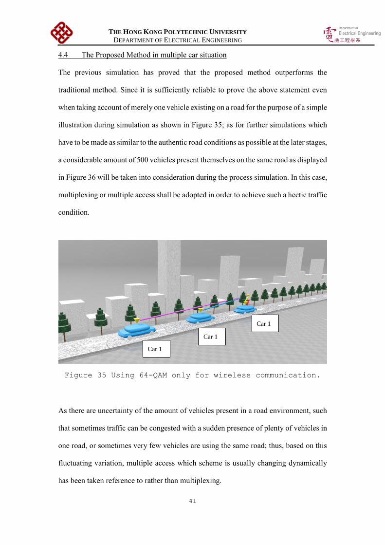
4.4 The Proposed Method in multiple car situation
The previous simulation has proved that the proposed method outperforms the
traditional method. Since it is sufficiently reliable to prove the above statement even
when taking account of merely one vehicle existing on a road for the purpose of a simple
illustration during simulation as shown in Figure 35; as for further simulations which
have to be made as similar to the authentic road conditions as possible at the later stages,
a considerable amount of 500 vehicles present themselves on the same road as displayed
in Figure 36 will be taken into consideration during the process simulation. In this case,
multiplexing or multiple access shall be adopted in order to achieve such a hectic traffic
condition.
Figure 35 Using 64-QAM only for wireless communication.
As there are uncertainty of the amount of vehicles present in a road environment, such
that sometimes traffic can be congested with a sudden presence of plenty of vehicles in
one road, or sometimes very few vehicles are using the same road; thus, based on this
fluctuating variation, multiple access which scheme is usually changing dynamically
has been taken reference to rather than multiplexing.
Car 1
Car 1
Car 1

THE HONG KONG POLYTECHNIC UNIVERSITY
DEPARTMENT OF ELECTRICAL ENGINEERING
42
Figure 36 Using 64-QAM only for wireless communication.
Nonetheless, when opting to utilize the traditional time division multiple access method,
notwithstanding a time division in an equal manner, since the proposed method has
adopted QAM4, QAM16, and QAM64 respectively for maximizing the efficiency of
the communication, as a consequence, this multiple access method is not appropriate to
apply to the proposed method due to the unfair receival of data among the vehicles on
the same road in a specific time frame with reference to each of their distance from the
road-base transmitter, such that the closer the distance between the vehicle and the
transmitter, the greater the amount of information that the vehicle will receive, and the
vice versa.
In light of it, the weakness of the traditional method resulting in an unfairness received
of data among the vehicles will be overcome by a tailor-made method proposed in this
report. In the specifically designed method, time will be allocated according to the
relative proportions of QAM4, QAM16, and QAM64 respectively and the
corresponding number of vehicles under QAM4, QAM16, and QAM64 respectively.
Car 1
Car 2
Car 3
Car 4
Car 5

THE HONG KONG POLYTECHNIC UNIVERSITY
DEPARTMENT OF ELECTRICAL ENGINEERING
43
The equation is as follows.
Assumption 1: The time allocated for and number of vehicles under 4-QAM
transmission are A and X respectively
Assumption 2: The time allocated for and number of vehicles under 16-QAM
transmission are B and Y respectively
Assumption 3: The time allocated for and number of vehicles under 64-QAM
transmission are C and Z respectively
For one second time slot,
A × X + B × Y + C × Z = 1
For equal data received
Log2(4) × A = Log2(16) × B = Log2(64) × C
Therefore,
Time allocated for vehicles under 4-QAM = 2
2X+Y+2
3Z
Time allocated for vehicles under 16-QAM = 1
2X+Y+2
3Z
Time allocated for vehicles under 64-QAM = 2
6X+3Y+2Z

THE HONG KONG POLYTECHNIC UNIVERSITY
DEPARTMENT OF ELECTRICAL ENGINEERING
44
Through using the designed method, every vehicle exists on the same road can be able
to receive the same amount of data regardless of the variations in the distance between
the vehicle and the transmitter when compared with the conventional method. The
difference between the designed method and traditional method is clearly shown in
Figure 37.
When there are 500 vehicles passing through the same road in order to receive the data
from the transmitter, yet only the vehicles in the middle of the road can reflect the
conditions of the traffic stream, therefore, merely 45 vehicles situated in the middle will
be taken into account for the simulation, then the data that these 45 vehicles have
received from the transmitter in one second when they are in the transmitting range of
the transmitter are recorded.
It should be noted that the first and last few vehicles out of the 45 vehicle sample do
not receive any data since they are without the transmitting range.
Figure 37 Received Data among 45 cars for a time slot.
THE HONG KONG POLYTECHNIC UNIVERSITY
DEPARTMENT OF ELECTRICAL ENGINEERING
45
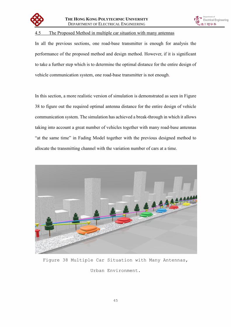
4.5 The Proposed Method in multiple car situation with many antennas
In all the previous sections, one road-base transmitter is enough for analysis the
performance of the proposed method and design method. However, if it is significant
to take a further step which is to determine the optimal distance for the entire design of
vehicle communication system, one road-base transmitter is not enough.
In this section, a more realistic version of simulation is demonstrated as seen in Figure
38 to figure out the required optimal antenna distance for the entire design of vehicle
communication system. The simulation has achieved a break-through in which it allows
taking into account a great number of vehicles together with many road-base antennas
“at the same time” in Fading Model together with the previous designed method to
allocate the transmitting channel with the variation number of cars at a time.
Figure 38 Multiple Car Situation with Many Antennas,
Urban Environment.

THE HONG KONG POLYTECHNIC UNIVERSITY
DEPARTMENT OF ELECTRICAL ENGINEERING
46
The result of the simulation for different vehicular speeds with required data is shown
below in Figure 39 with an assumption of 10 MB received data in 1000m long vehicle
travel distance in Rayleigh Fading Model or just say in urban area.
Figure 39 Optimal Antenna Distance in Rayleigh Fading.
It is observed that the optimal antenna distance decreases with increasing vehicular
speed. When it comes to zero, that means the entire vehicle commutation system cannot
provide the required data at such vehicular speed. As a result, if drivers want to receive
such an amount of data, they have to slow down the vehicular speed.
Despite the fact that the system cannot meet the requirement at 70km/hr or above, it is
noted that in general vehicular speed is not as high as 70 km/hr in urban area excluding
highway. Therefore, it is still appropriate to adopt the designed system in reality.

THE HONG KONG POLYTECHNIC UNIVERSITY
DEPARTMENT OF ELECTRICAL ENGINEERING
47
The same applies to Rician Fading Model or rural areas as seen in Figure 40.
Figure 40 Multiple Car Situation with Many Antennas,
Rural Environment.
The result in Figure 41 shows that the design system is appropriate in reality for rural
case including highway with high vehicular speed.
Figure 41 Optimal Antenna Distance in Rician Fading
THE HONG KONG POLYTECHNIC UNIVERSITY
DEPARTMENT OF ELECTRICAL ENGINEERING
48
5 Conclusion and Future Development
5.1 Conclusion
From above simulation results, it is concluded that the proposed method is superior to
traditional methods in both Rayleigh Fading Model and Rician Fading Model. Under
the same transmit power, there is a significant improvement in total bits at the receiver
end for varying speeds, which means moving vehicles can obtain more information
from the network through the proposed method.
After the recognition of the performance of the proposed method, it is then put into
practice by adopting adjustments for the purpose of designing a well-rounded vehicle
communication system. The adjustment is allocating the transmitting channel through
a new time-division multiple access method such that every vehicle exists on the same
road can be able to receive the same amount of data regardless of the variations in the
distance between the vehicle and the transmitter when compared with the conventional
method.
Last but not least, the result of simulation of applying the design vehicle communication
system in a more realistic road environment reflects that the design system is
appropriate to be utilized in reality. The optimal antenna distance obtained in the
simulation provided the best indication for placing the antenna, which is conducive to
reducing the social cost of and time required for numerous trials of various distances in
practice.

THE HONG KONG POLYTECHNIC UNIVERSITY
DEPARTMENT OF ELECTRICAL ENGINEERING
49
5.2 Limitation
The KLOS factor varies with the road environment, while it exerts a significant impact
on the path channel loss, thus affecting the design of the system. Since there exists a
large variation in the KLOS factor corresponding to different road conditions, only two
assumptions of KLOS factor are adopted in this report for simulation purpose. It is
recommended that if this system is to be applied in the real situation, independent
measurement of KLOS factor for each road should be conducted.
5.3 Future Development
As the simulation reflected that the proposed method is definitely feasible, it provides
a basis for a future experiment taken account of factors and variation aplenty existed in
an authentic environment with the aid of raw Wi-Fi transmitters and receivers, so that
the proposed method can be further examined whether it will be viable in practice.

THE HONG KONG POLYTECHNIC UNIVERSITY
DEPARTMENT OF ELECTRICAL ENGINEERING
50
6 References
[1] M. Sivak and B. Schoettle, “Road safety with self-driving vehicles: General
limitations and road sharing with conventional vehicles,” pp. 1–13, Jan. 2015.
[2] Chapter 8 of A. V. Oppenheim and A. S. Willsky, Signals and Systems. Prentice
Hall, 1997.
[3] B. Hassibi and B. Hochwald, “How much training is needed in multiple-
antenna wireless links,” IEEE Transactions on Information Theory, vol. 49, no.
4, pp. 951–963, 2003.
[4] V. Tarokh, N. Seshadri, and A. Calderbank, “Space-time codes for high data
rate wireless communication: performance criterion and code construction,”
IEEE Transactions on Information Theory, vol. 44, no. 2, pp. 744–765, 1998.
[5] E. Biglieri, “High-Level Modulation and Coding for Nonlinear Satellite
Channels,” IEEE Transactions on Communications, vol. 32, no. 5, pp. 616–626,
1984.
[6] J. Christopher L, “Method of adding encryption/encoding element to the
modulation/demodulation process,” U.S. Patent No. 6,157,679, pp. 1–8, Dec.
2000.
[7] S. Claude Elwood, “Communication in the presence of noise,” Proceedings of
the IRE, vol. 37, no. 1, pp. 10–21, 1949.
[8] Chapter 5 of S. Haykin and M. Moher, Communication systems. New York:
John Wiley & Sons, 2010.
[9] A. Watt and E. Maxwell, “Characteristics of Atmospheric Noise from 1 to 100
KC,” Proceedings of the IRE, vol. 45, no. 6, pp. 787–794, 1957.
[10] Chapter 7,8 of S. Haykin and M. Moher, Communication systems. New York:
John Wiley & Sons, 2010.
[11] Chapter 3 of J. Gerrits, Wideband FM techniques for low-power wireless
communications. Gistrup: River Publishers, 2016.
[12] Chapter 4 of S. Haykin and M. Moher, Communication systems. New York:
John Wiley & Sons, 2010.
[13] Chapter 2 of D. Tse and P. Viswanath, Fundamentals of wireless communication.
Cambridge UP: Cambridge, 2013.
[14] Chapter 2 of A. Goldsmith, Wireless Communications. Cambridge University
Press, 2005.
[15] Chapter 4 of A. Aragon-Zavala, Indoor wireless communications: from theory
to implementation. Hoboken, NJ: John Wiley & Sons, Inc., 2017.

THE HONG KONG POLYTECHNIC UNIVERSITY
DEPARTMENT OF ELECTRICAL ENGINEERING
51
[16] K. Chetcuti, C. J. Debono, and S. Bruillot, “The effect of human shadowing on
RF signal strengths of IEEE802.11a systems on board business jets,” 2010 IEEE
Aerospace Conference, 2010.
[17] Chapter 2 of J. J. Carr and G. W. Hippisley, Practical antenna handbook. New
York: McGraw-Hill, 2012.
[18] A. Al-Barrak, A. Al-Sherbaz, T. Kanakis, and R. Crockett, “Enhancing BER
Performance Limit of BCH and RS Codes Using Multipath Diversity,”
Computers, vol. 6, no. 4, p. 21, 2017.
[19] Chapter 20 of A. F. Molisch, Wireless communications. Chichester: John Wiley
& Sons, 2011.
[20] Chapter 8 of A. Weintrit, Navigational problems: marine navigation and safety
of sea transportation. Leiden: CRC Press/Balkema, 2013.
[21] Chapter 11of B. Sklar, Digital communications: fundamentals and applications.
Prentice Hall PTR, 2017.
[22] Chapter 6 of B. P. Lathi and Z. Ding, Modern digital and analog communication
systems. New York: Oxford Univ Press, 2010.
[23] M. Hasna and M.-S. Alouini, “End-to-end performance of transmission systems
with relays over rayleigh-fading channels,” IEEE Transactions on Wireless
Communications, vol. 2, no. 6, pp. 1126–1131, 2003.
[24] Y.-D. Yao and A. Sheikh, “Outage probability analysis for microcell mobile
radio systems with cochannel interferers in Rician/Rayleigh fading
environment,” Electronics Letters, vol. 26, no. 13, p. 864, 1990.
[25] S. Zhu, T. S. Ghazaany, S. M. R. Jones, R. A. Abd-Alhameed, J. M. Noras, T. V.
Buren, J. Wilson, T. Suggett, and S. Marker, “Probability Distribution of Rician
K-Factor in Urban, Suburban and Rural Areas Using Real-World Captured
Data,” IEEE Transactions on Antennas and Propagation, vol. 62, no. 7, pp.
3835–3839, 2014.
[26] Z. Xu, X. Li, X. Zhao, M. H. Zhang, and Z. Wang, “DSRC versus 4G-LTE for
Connected Vehicle Applications: A Study on Field Experiments of Vehicular
Communication Performance,” Journal of Advanced Transportation, vol. 2017,
pp. 1–10, 2017.
[27] “ALLOWABLE ERROR PERFORMANCE FOR A HYPOTHETICAL
REFERENCE DIGITAL PATH IN THE FIXED-SATELLITE SERVICE
OPERATING BELOW 15 GHz WHEN FORMING PART OF AN
INTERNATIONAL CONNECTION IN AN INTEGRATED SERVICES
DIGITAL NETWORK,” RECOMMENDATION ITU-R S.614-3. [Online].
Available: https://www.itu.int/dms_pubrec/itu-r/rec/s/R-REC-S.614-3-199409-
S!!PDF-E.pdf.

THE HONG KONG POLYTECHNIC UNIVERSITY
DEPARTMENT OF ELECTRICAL ENGINEERING
52
7 Appendix
7.1.1 Generation of BER against SNR for 4-QAM, 16-QAM, 64-QAM
function [y ] = QAM(Order)
SNR_dB=0:40;
NumberSNR=length(SNR_dB);
BER=zeros(1,NumberSNR);
N=10^6; % No. of Sample
Scale=2*(Order-1)/3;
PositionFactor=sqrt(1/Scale);
Qam4=[-1,1];
Qam16=[-3,-1,1,3];
Qam64=[-7,-5,-3,-1,1,3,5,7];
if Order==4
Alphabet=Qam4;
Upperlimit=1*PositionFactor;
Lowerlimit=-1*PositionFactor;
a='mx-';
elseif Order==16
Alphabet=Qam16;
Upperlimit=3*PositionFactor;
Lowerlimit=-3*PositionFactor;
a='bx-';
elseif Order==64
Alphabet=Qam64;
Upperlimit=7*PositionFactor;
Lowerlimit=-7*PositionFactor;
a='gx-';
end
Signal=PositionFactor*(randsrc(1,N,Alphabet)+1i*randsrc(1,N,Alphabet));
SignalRealPart=real(Signal);
SignalImagPart=imag(Signal);
NoiseSource=randn(1,N)+1i*randn(1,N);

THE HONG KONG POLYTECHNIC UNIVERSITY
DEPARTMENT OF ELECTRICAL ENGINEERING
53
for i=1:NumberSNR
SNR=10^(SNR_dB(i)/10); % SNR_dB -> SNR
Sigma=sqrt(1/(2*SNR)); % Sigma for Complex Case
Noise=Sigma*NoiseSource; % Additive White Noise
y=Signal+Noise;
yRealPart=real(y);
yImagPart=imag(y);
DistanceReal=abs(SignalRealPart-yRealPart);
DistanceImag=abs(SignalImagPart-yImagPart);
count=0;
for n=1:N
if yRealPart(1,n)>Upperlimit || yRealPart (1,n)<Lowerlimit
if yImagPart(1,n)>Upperlimit ||yImagPart(1,n)<Lowerlimit
else
ImagExistError=DistanceImag(1,n)==PositionFactor ||
DistanceImag(1,n)>PositionFactor;
if ImagExistError==1
count=count+1;
else
RealExistError=DistanceReal(1,n)==PositionFactor ||
DistanceReal(1,n)>PositionFactor;
if RealExistError==1
count=count+1;
end
end
end
end
end
NoError=count;
BER(1,i)=NoError/N;
end
semilogy(SNR_dB,BER,a)
xlabel('SNR (dB) ');
ylabel('BER');
title('BER against SNR simulation for 4-QAM, 16-QAM and 64-QAM');

THE HONG KONG POLYTECHNIC UNIVERSITY
DEPARTMENT OF ELECTRICAL ENGINEERING
54
if Order==4
legend('4-QAM');
elseif Order==16
legend('16-QAM');
elseif Order==64
legend('64-QAM');
end
hold on
end
7.1.2 Plot BER against SNR for 4-QAM, 16-QAM, 64-QAM
function [] = Plot(Number)
%UNTITLED Summary of this function goes here
% Detailed explanation goes here
if Number==1
QAM(4);
legend('4-QAM');
elseif Number==2
QAM(4);
QAM(16);
legend('4-QAM','16-QAM');
elseif Number==3
QAM(4);
QAM(16);
QAM(64);
legend('4-QAM','16-QAM','64-QAM');
end
end

THE HONG KONG POLYTECHNIC UNIVERSITY
DEPARTMENT OF ELECTRICAL ENGINEERING
55
7.2.1 Generation of BER against SNR for 4-QAM, 16-QAM, 64-QAM (Fading
Model)
function [y ] = QAM_Fading(Order,K)
SNR_dB=0:70;
NumberSNR=length(SNR_dB);
BER=zeros(1,NumberSNR);
N=10^6; % No. of Sample
Scale=2*(Order-1)/3;
PositionFactor=sqrt(1/Scale);
Qam4=[-1,1];
Qam16=[-3,-1,1,3];
Qam64=[-7,-5,-3,-1,1,3,5,7];
if Order==4
Alphabet=Qam4;
Upperlimit=1*PositionFactor;
Lowerlimit=-1*PositionFactor;
a='mx-';
elseif Order==16
Alphabet=Qam16;
Upperlimit=3*PositionFactor;
Lowerlimit=-3*PositionFactor;
a='bx-';
elseif Order==64
Alphabet=Qam64;
Upperlimit=7*PositionFactor;
Lowerlimit=-7*PositionFactor;
a='gx-';
end
Signal=PositionFactor*(randsrc(1,N,Alphabet)+1i*randsrc(1,N,Alphabet));
SignalRealPart=real(Signal);
SignalImagPart=imag(Signal);
if K==0
THE HONG KONG POLYTECHNIC UNIVERSITY
DEPARTMENT OF ELECTRICAL ENGINEERING
56
RayleighFading=1/sqrt(2)*(randn(1,N)+1i*randn(1,N));
Fading=RayleighFading;
else
RicianFading=sqrt(K/(K+1))+sqrt(1/(K+1))*1/sqrt(2)*(randn(1,N)+1i*randn(1,N));
Fading=RicianFading;
end
NoiseSource=randn(1,N)+1i*randn(1,N);
for i=1:NumberSNR
SNR=10^(SNR_dB(i)/10); % SNR_dB -> SNR
Sigma=sqrt(1/(2*SNR)); % Sigma for Complex Case
Noise=Sigma*NoiseSource; % Additive White Noise
% Received Signal
y=Fading.*Signal+Noise;
%Equalization: Remove Fading Effects
y=y./Fading;
%Demodulation
yRealPart=real(y);
yImagPart=imag(y);
DistanceReal=abs(SignalRealPart-yRealPart);
DistanceImag=abs(SignalImagPart-yImagPart);
count=0;
for n=1:N
if yRealPart(1,n)>Upperlimit || yRealPart (1,n)<Lowerlimit
if yImagPart(1,n)>Upperlimit ||yImagPart(1,n)<Lowerlimit
else
ImagExistError=DistanceImag(1,n)==PositionFactor ||
DistanceImag(1,n)>PositionFactor;
if ImagExistError==1
count=count+1;
else
RealExistError=DistanceReal(1,n)==PositionFactor ||
DistanceReal(1,n)>PositionFactor;
if RealExistError==1
THE HONG KONG POLYTECHNIC UNIVERSITY
DEPARTMENT OF ELECTRICAL ENGINEERING
57
count=count+1;
end
end
end
end
end
NoError=count;
BER(1,i)=NoError/N;
end
semilogy(SNR_dB,BER,a)
xlabel('SNR (dB) ');
ylabel('BER');
if K==0
title('BER against SNR simulation in Rayleigh fading for 4-QAM, 16-QAM and
64-QAM');
else
title('BER against SNR simulation in Rician fading for 4-QAM, 16-QAM and 64-
QAM');
end
if Order==4
legend('4-QAM');
elseif Order==16
legend('16-QAM');
elseif Order==64
legend('64-QAM');
end
hold on
end
THE HONG KONG POLYTECHNIC UNIVERSITY
DEPARTMENT OF ELECTRICAL ENGINEERING
58
7.2.2 Plot BER against SNR for 4-QAM, 16-QAM, 64-QAM ( Fading Model )
function [] = Plot_Fading(Number,K)
if Number==1
QAM_Fading(4,K);
legend('4-QAM');
elseif Number==2
QAM_Fading(4,K);
QAM_Fading(16,K);
legend('4-QAM','16-QAM');
elseif Number==3
QAM_Fading(4,K);
QAM_Fading(16,K);
QAM_Fading(64,K);
legend('4-QAM','16-QAM','64-QAM');
end
end
7.3.1 Distance Function
function distance = distance(kmPerHour,time)
NormalDistance=2;
mPerS=kmPerHour*1000/3600;
TravelDistance=mPerS*time;
distance=sqrt(TravelDistance^2+NormalDistance^2);
end
7.3.2 SNR dB Function
function SNRdB = SNRdB(distance)
Wavelength=0.05;
Bandwidth=75*10^6;
Ptx=1; %
T=290; %for room temperatere
k=1.38*10^(-23); %Boltzman Constant
Gtx=1; % Transmiter antenna gain for isotropic
Grx=1; % Reciever antenna gain for isotropic
THE HONG KONG POLYTECHNIC UNIVERSITY
DEPARTMENT OF ELECTRICAL ENGINEERING
59
SNR=(Ptx*Gtx*Grx*Wavelength^2)/(k*T*Bandwidth*(4*pi*distance)^2);
SNRdB=10*log10(SNR);
end
7.3.3 BER Function
function BER = QAM_BER(Order,K,SNR_dB)
N=10^6; % No. of Sample
Scale=2*(Order-1)/3;
PositionFactor=sqrt(1/Scale);
Qam4=[-1,1];
Qam16=[-3,-1,1,3];
Qam64=[-7,-5,-3,-1,1,3,5,7];
if Order==4
Alphabet=Qam4;
Upperlimit=1*PositionFactor;
Lowerlimit=-1*PositionFactor;
elseif Order==16
Alphabet=Qam16;
Upperlimit=3*PositionFactor;
Lowerlimit=-3*PositionFactor;
elseif Order==64
Alphabet=Qam64;
Upperlimit=7*PositionFactor;
Lowerlimit=-7*PositionFactor;
end
Signal=PositionFactor*(randsrc(1,N,Alphabet)+1i*randsrc(1,N,Alphabet));
SignalRealPart=real(Signal);
SignalImagPart=imag(Signal);
if K==0
RayleighFading=1/sqrt(2)*(randn(1,N)+1i*randn(1,N));

THE HONG KONG POLYTECHNIC UNIVERSITY
DEPARTMENT OF ELECTRICAL ENGINEERING
60
Fading=RayleighFading;
else
RicianFading=sqrt(K/(K+1))+sqrt(1/(K+1))*1/sqrt(2)*(randn(1,N)+1i*randn(1,N));
Fading=RicianFading;
end
NoiseSource=randn(1,N)+1i*randn(1,N);
SNR=10^(SNR_dB/10); % SNR_dB -> SNR
Sigma=sqrt(1/(2*SNR)); % Sigma for Complex Case
Noise=Sigma*NoiseSource; % Additive White Noise
% Received Signal
y=Fading.*Signal+Noise;
%Equalization: Remove Fading Effects
y=y./Fading;
%Demodulation
yRealPart=real(y);
yImagPart=imag(y);
DistanceReal=abs(SignalRealPart-yRealPart);
DistanceImag=abs(SignalImagPart-yImagPart);
count=0;
for n=1:N
if yRealPart(1,n)>Upperlimit || yRealPart (1,n)<Lowerlimit
if yImagPart(1,n)>Upperlimit ||yImagPart(1,n)<Lowerlimit
else
ImagExistError=DistanceImag(1,n)==PositionFactor ||
DistanceImag(1,n)>PositionFactor;
if ImagExistError==1
count=count+1;
else
RealExistError=DistanceReal(1,n)==PositionFactor ||
DistanceReal(1,n)>PositionFactor;
if RealExistError==1
count=count+1;
end

THE HONG KONG POLYTECHNIC UNIVERSITY
DEPARTMENT OF ELECTRICAL ENGINEERING
61
end
end
end
end
NoError=count;
BER=NoError/N;
end
7.3.4 QAM Order Function
function Order = QAM_Order_ForGivenSNR(K,SNR_dB,Method)
BerLimit=10^-3;
if Method==0
BER64=QAM_BER(64,K,SNR_dB);
if BER64<BerLimit || BER64==BerLimit
Order=64;
else
BER16=QAM_BER(16,K,SNR_dB);
if BER16<BerLimit || BER16==BerLimit
Order=16;
else
BER4=QAM_BER(4,K,SNR_dB);
if BER4<BerLimit || BER4==BerLimit
Order=4;
else
Order=0;
end
end
end
elseif Method==4
BER4=QAM_BER(4,K,SNR_dB);
if BER4<BerLimit || BER4==BerLimit
Order=4;
else
Order=0;
end

THE HONG KONG POLYTECHNIC UNIVERSITY
DEPARTMENT OF ELECTRICAL ENGINEERING
62
elseif Method==16
BER16=QAM_BER(16,K,SNR_dB);
if BER16<BerLimit || BER16==BerLimit
Order=16;
else
Order=0;
end
elseif Method==64
BER64=QAM_BER(64,K,SNR_dB);
if BER64<BerLimit || BER64==BerLimit
Order=64;
else
Order=0;
end
end
7.3.5 Bits Rate Function
function BitRate = Bit_Rate(Order)
if Order==0
BitRate=0;
else
Bandwidth=75/2*10^6;
BitRate=log2(Order)*Bandwidth/10^9;
end
7.3.6 Total Bits Function
function TotalBit = Total_Bit(kmPerHour,K,Method)
Bit=0;
for time=1:120
Distance= distance(kmPerHour,time);
SNR_dB = SNRdB(Distance);
Order = QAM_Order_ForGivenSNR(K,SNR_dB,Method);
if Order==0
break

THE HONG KONG POLYTECHNIC UNIVERSITY
DEPARTMENT OF ELECTRICAL ENGINEERING
63
else
count = Bit_Rate(Order);
Bit=Bit+count;
end
end
TotalBit=Bit*2;
End
7.3.7 Plot Total Bits against Speed Function
function [] = Plot_TotalBit_Against_Speed(K,Method)
a=zeros(1,7);
b=20:10:80;
for kmPerHour=20:10:80
TotalBit = Total_Bit(kmPerHour,K,Method);
a(kmPerHour/10-1)=TotalBit;
if Method==0
if K==0
title('Total Bits against Speed in Rayleigh Fading');
else
title('Total Bits against Speed in Rician Fading');
end
elseif Method==4
if K==0
title('Total Bits against Speed in Rayleigh Fading, 4-QAM only');
else
title('Total Bits against Speed in Rician Fading, 4-QAM only');
end
elseif Method==16
if K==0
title('Total Bits against Speed in Rayleigh Fading, 16-QAM only');
else
title('Total Bits agaisnt Speed in Rician Fading, 16-QAM only');
end
elseif Method==64
if K==0
THE HONG KONG POLYTECHNIC UNIVERSITY
DEPARTMENT OF ELECTRICAL ENGINEERING
64
title('Total Bits against Speed in Rayleigh Fading, 64-QAM only');
else
title('Total Bits against Speed in Rician Fading, 64-QAM only');
end
end
end
if Method==0
plot(b,a,'-kx');
elseif Method==4
plot(b,a,'-mx');
elseif Method==16
plot(b,a,'-bx');
elseif Method==64
plot(b,a,'-gx');
end
axis([15,85,1.5,25]);
xlabel('Speed (km/h)');
ylabel('Total Bits (Gbits)')
set(gca,'fontsize',15)
hold on
end
7.3.8 Plot ALL Type Total Bits against Speed Function
function [] = Plot_ALL_TotalBit_Against_Speed(K,Number)
if Number==3
Plot_TotalBit_Against_Speed(K,4)
Plot_TotalBit_Against_Speed(K,16)
Plot_TotalBit_Against_Speed(K,64)
if K==0
title('Total Bits against Speed in Rayleigh Fading for 4-QAM, 16-QAM, 64-
QAM');
else
title('Total Bits against Speed in Rician Fading for 4-QAM, 16-QAM, 64-
QAM');
end
legend('4-QAM','16-QAM','64-QAM');

THE HONG KONG POLYTECHNIC UNIVERSITY
DEPARTMENT OF ELECTRICAL ENGINEERING
65
elseif Number==4
Plot_TotalBit_Against_Speed(K,0)
Plot_TotalBit_Against_Speed(K,4)
Plot_TotalBit_Against_Speed(K,16)
Plot_TotalBit_Against_Speed(K,64)
if K==0
title('Total Bits against Speed in Rayleigh Fading for Proposed Method');
else
title('Total Bits against Speed in Rician Fading for Proposed Method');
end
legend('Proposed Method','4-QAM','16-QAM','64-QAM');
end
end
7.4.1 Create Car Start Point Function
function CarStartPoint = Create_CarStartPoint(CarNumber,CarBetweenDistance)
StartPoint=-2000;
CarStartPoint=zeros(1,CarNumber);
CarVariations=zeros(1,CarNumber);
for n=1:CarNumber
while CarVariations(1,n) <5
CarVariations(1,n)=randn(1)*CarBetweenDistance;
if CarVariations(1,n)==0
CarVariations(1,n)=CarBetweenDistance;
end
end
end
for n=1:CarNumber
CarStartPoint(1,n)=StartPoint-CarVariations(1,n);
StartPoint=CarStartPoint(1,n);
end
end
7.4.2 Distance km/hr to m/s unit Function
function distance = distance_kmTOmUnit(kmPerHour,time)
mPerS=kmPerHour*1000/3600;

THE HONG KONG POLYTECHNIC UNIVERSITY
DEPARTMENT OF ELECTRICAL ENGINEERING
66
distance=mPerS*time;
end
7.4.2 Check Car QAM Order Function
function CarQAM =
Advanced_Car_QAM(Location,QAM4Distance,QAM16Distance,QAM64Distance)
CarQAM=zeros(1,3);
QAM4CAR=0;
QAM16CAR=0;
QAM64CAR=0;
if (Location>-QAM4Distance || Location==-QAM4Distance) && Location<-
QAM16Distance
QAM4CAR=1;
elseif (Location>-QAM16Distance || Location==-QAM16Distance) && Location<-
QAM64Distance
QAM16CAR=1;
elseif (Location>-QAM64Distance || Location==-QAM64Distance) &&
(Location<QAM64Distance || Location==QAM64Distance)
QAM64CAR=1;
elseif Location>QAM64Distance && (Location<QAM16Distance ||
Location==QAM16Distance)
QAM16CAR=1;
elseif Location>QAM16Distance && (Location<QAM4Distance ||
Location==QAM4Distance)
QAM4CAR=1;
end
CarQAM(1,1)=QAM4CAR;
CarQAM(1,2)=QAM16CAR;
CarQAM(1,3)=QAM64CAR;
THE HONG KONG POLYTECHNIC UNIVERSITY
DEPARTMENT OF ELECTRICAL ENGINEERING
67
7.4.3 Traditional Time Division Method Function
function BitCountPerCar =
Traditional_Time(CarInsideRange4QAM,CarInsideRange16QAM,CarInsideRange64
QAM)
BitCountPerCar=zeros(1,3);
CarInsideRange=CarInsideRange4QAM + CarInsideRange16QAM +
CarInsideRange64QAM;
AllocatedTime=1/CarInsideRange;
if CarInsideRange4QAM==0
BitQAM4countPerCar =0;
else
BitQAM4countPerCar = Bit_Rate(4)*AllocatedTime;
end
if CarInsideRange16QAM==0
BitQAM16countPerCar =0;
else
BitQAM16countPerCar = Bit_Rate(16)*AllocatedTime;
end
if CarInsideRange64QAM==0
BitQAM64countPerCar =0;
else
BitQAM64countPerCar = Bit_Rate(64)*AllocatedTime;
end
BitCountPerCar(1,1)= BitQAM4countPerCar;
BitCountPerCar(1,2)= BitQAM16countPerCar;
BitCountPerCar(1,3)= BitQAM64countPerCar;
7.4.4 Designed Time Division Method Function
function BitCountPerCar =
Designed_Time(CarInsideRange4QAM,CarInsideRange16QAM,CarInsideRange64Q
AM)
BitCountPerCar=zeros(1,3);

THE HONG KONG POLYTECHNIC UNIVERSITY
DEPARTMENT OF ELECTRICAL ENGINEERING
68
if CarInsideRange4QAM==0
BitQAM4countPerCar =0;
else
QAM4AllocatedTime = 2/(2*CarInsideRange4QAM + CarInsideRange16QAM +
2/3*CarInsideRange64QAM);
BitQAM4countPerCar = Bit_Rate(4)*QAM4AllocatedTime;
end
if CarInsideRange16QAM==0
BitQAM16countPerCar =0;
else
QAM16AllocatedTime = 1/(2*CarInsideRange4QAM + CarInsideRange16QAM +
2/3*CarInsideRange64QAM);
BitQAM16countPerCar = Bit_Rate(16)*QAM16AllocatedTime;
end
if CarInsideRange64QAM==0
BitQAM64countPerCar =0;
else
QAM64AllocatedTime = 2/(6*CarInsideRange4QAM + 3*CarInsideRange16QAM
+ 2*CarInsideRange64QAM);
BitQAM64countPerCar = Bit_Rate(64)*QAM64AllocatedTime;
end
BitCountPerCar(1,1)= BitQAM4countPerCar;
BitCountPerCar(1,2)= BitQAM16countPerCar;
BitCountPerCar(1,3)= BitQAM64countPerCar;
7.4.5 Plot Traditional against Designed Time Division Method Function
function []= Plot_Traditonal_To_Design()
Data=load('UrbanArea.mat');
QAMAntennaDistance=Data. DifferetQAMAntennaDistance;
QAM4Distance=QAMAntennaDistance(1,1);
QAM16Distance=QAMAntennaDistance(1,2);
QAM64Distance=QAMAntennaDistance(1,3);
TimeSet=1000;

THE HONG KONG POLYTECHNIC UNIVERSITY
DEPARTMENT OF ELECTRICAL ENGINEERING
69
CarNumber=200;
CarBetweenDistance=20;
kmPerHour=20;
CarStartPoint = Create_CarStartPoint(CarNumber,CarBetweenDistance);
Location=CarStartPoint;
TimePeriod=1;
Distance = distance_kmTOmUnit(kmPerHour,TimePeriod);
Data=zeros(TimeSet,CarNumber);
for time=1:TimeSet
NumberOfCarForQAMPerTimeSlot=zeros(1,3);
for n=1:CarNumber
Location(1,n)=Location(1,n)+Distance;
CarCount=Advanced_Car_QAM(Location(1,n),QAM4Distance,QAM16Dista
nce,QAM64Distance);
if CarCount(1,1)>0
Data(time,n)=4;
elseif CarCount(1,2)>0
Data(time,n)=16;
elseif CarCount(1,3)>0
Data(time,n)=64;
end
NumberOfCarForQAMPerTimeSlot= NumberOfCarForQAMPerTimeSlot +
CarCount;
end
CarInsideRange4QAMPerTimeSlot =NumberOfCarForQAMPerTimeSlot(1,1);
CarInsideRange16QAMPerTimeSlot =NumberOfCarForQAMPerTimeSlot(1,2);
CarInsideRange64QAMPerTimeSlot =NumberOfCarForQAMPerTimeSlot(1,3);
BitCountPerCar =
Designed_Time(CarInsideRange4QAMPerTimeSlot,CarInsideRange16QAMPerTime
Slot,CarInsideRange64QAMPerTimeSlot);
for n=1:CarNumber
if Data(time,n)==4
Data(time,n)=BitCountPerCar(1,1);
elseif Data(time,n)==16
Data(time,n)=BitCountPerCar(1,2);
elseif Data(time,n)==64

THE HONG KONG POLYTECHNIC UNIVERSITY
DEPARTMENT OF ELECTRICAL ENGINEERING
70
Data(time,n)=BitCountPerCar(1,3);
end
end
end
% Measure 45 Cars for Comparing
NthCar=zeros(45,2);
for time=1:TimeSet
if Data(time,100)>0
for n=1:45
Car=60+n;
NthCar(n,1)=Data(time,Car)*1024^2/8;
end
break
end
end
title('KiloBytes against Car in Design VS Traditional System, 45 Cars');
xlabel('Nth Car');
ylabel('KaloByes(KB/s)')
set(gca,'fontsize',15)
hold on
Location=CarStartPoint;
TimePeriod=1;
Distance = distance_kmTOmUnit(kmPerHour,TimePeriod);
Data=zeros(TimeSet,CarNumber);
for time=1:TimeSet
NumberOfCarForQAMPerTimeSlot=zeros(1,3);
for n=1:CarNumber
Location(1,n)=Location(1,n)+Distance;
CarCount=Advanced_Car_QAM(Location(1,n),QAM4Distance,QAM16Dista
nce,QAM64Distance);
if CarCount(1,1)>0

THE HONG KONG POLYTECHNIC UNIVERSITY
DEPARTMENT OF ELECTRICAL ENGINEERING
71
Data(time,n)=4;
elseif CarCount(1,2)>0
Data(time,n)=16;
elseif CarCount(1,3)>0
Data(time,n)=64;
end
NumberOfCarForQAMPerTimeSlot= NumberOfCarForQAMPerTimeSlot +
CarCount;
end
CarInsideRange4QAMPerTimeSlot =NumberOfCarForQAMPerTimeSlot(1,1);
CarInsideRange16QAMPerTimeSlot =NumberOfCarForQAMPerTimeSlot(1,2);
CarInsideRange64QAMPerTimeSlot =NumberOfCarForQAMPerTimeSlot(1,3);
BitCountPerCar =
Traditional_Time(CarInsideRange4QAMPerTimeSlot,CarInsideRange16QAMPerTim
eSlot,CarInsideRange64QAMPerTimeSlot);
for n=1:CarNumber
if Data(time,n)==4
Data(time,n)=BitCountPerCar(1,1);
elseif Data(time,n)==16
Data(time,n)=BitCountPerCar(1,2);
elseif Data(time,n)==64
Data(time,n)=BitCountPerCar(1,3);
end
end
end
for time=1:TimeSet
if Data(time,100)>0
for n=1:45
Car=60+n;
NthCar(n,2)=Data(time,Car)*1024^2/8;
end
break
end
end
bar(NthCar);

THE HONG KONG POLYTECHNIC UNIVERSITY
DEPARTMENT OF ELECTRICAL ENGINEERING
72
%axis([60,110,0,0.008]);
xlabel('Nth Car');
ylabel('KiloBytes(KB/s)')
set(gca,'fontsize',15)
legend('Designed Method','Traditional Method');
hold on
7.5.1 Advanced Car QAM Order with Many Antennas Function
function CarQam =
Advanced_CarQAM_WithManyAntenna(Location,AntennaDistance,QAM4Distance,
QAM16Distance,QAM64Distance)
CarQam=zeros(1,3);
NumberOfAntenna=10;
LastAntennaLocation=AntennaDistance*NumberOfAntenna;
QAM4CAR=0;
QAM16CAR=0;
QAM64CAR=0;
Run=1;
if (Location>-QAM4Distance || Location==-QAM4Distance) && Location<-
QAM16Distance
QAM4CAR=1;
elseif (Location>-QAM16Distance || Location==-QAM16Distance) && Location<-
QAM64Distance
QAM16CAR=1;
elseif (Location>-QAM64Distance || Location==-QAM64Distance) && Location<0
QAM4CAR=1;
end
if (Location==0|| Location>0) && (Location<AntennaDistance/2 ||
Location==AntennaDistance/2)
if (AntennaDistance/2 >0 ) && (AntennaDistance/2 <QAM64Distance ||
AntennaDistance/2==QAM64Distance )
if (Location==0 || Location >0 ) && (Location <AntennaDistance/2 ||
Location==AntennaDistance/2 )
QAM64CAR=1;
end
THE HONG KONG POLYTECHNIC UNIVERSITY
DEPARTMENT OF ELECTRICAL ENGINEERING
73
elseif AntennaDistance/2>QAM64Distance && (AntennaDistance/2
<QAM16Distance || AntennaDistance/2==QAM16Distance )
if (Location==0 || Location >0 ) && (Location <QAM64Distance ||
Location==QAM64Distance )
QAM64CAR=1;
elseif (Location >QAM64Distance ) && (Location <AntennaDistance/2 ||
Location==AntennaDistance/2 )
QAM16CAR=1;
end
elseif AntennaDistance/2>QAM16Distance
if (Location==0 || Location >0 ) && (Location <QAM64Distance ||
Location==QAM64Distance )
QAM64CAR=1;
elseif (Location >QAM64Distance ) && (Location <QAM16Distance ||
Location==QAM16Distance )
QAM16CAR=1;
elseif (Location >QAM16Distance ) && (Location <AntennaDistance/2 ||
Location==AntennaDistance/2 )
QAM4CAR=1;
end
end
end
if Location>AntennaDistance/2 && (Location<LastAntennaLocation ||
Location==LastAntennaLocation)
while Run==1
Difference=abs(Location-AntennaDistance);
if Difference<AntennaDistance/2 || Difference==AntennaDistance/2
if (AntennaDistance/2 >0 ) && (AntennaDistance/2 <QAM64Distance ||
AntennaDistance/2==QAM64Distance )
if (Difference==0 || Difference >0 ) && (Difference <AntennaDistance/2 ||
Difference==AntennaDistance/2 )
QAM64CAR=1;
end
elseif AntennaDistance/2>QAM64Distance && (AntennaDistance/2
<QAM16Distance || AntennaDistance/2==QAM16Distance )
if (Difference==0 || Location >0 ) && (Difference <QAM64Distance ||
Difference==QAM64Distance )

THE HONG KONG POLYTECHNIC UNIVERSITY
DEPARTMENT OF ELECTRICAL ENGINEERING
74
QAM64CAR=1;
elseif (Difference >QAM64Distance ) && (Difference <AntennaDistance/2
|| Difference==AntennaDistance/2 )
QAM16CAR=1;
end
elseif AntennaDistance/2>QAM16Distance
if (Difference==0 || Difference >0 ) && (Difference <QAM64Distance ||
Difference==QAM64Distance )
QAM64CAR=1;
elseif (Difference >QAM64Distance ) && (Difference <QAM16Distance ||
Difference==QAM16Distance )
QAM16CAR=1;
elseif (Difference >QAM16Distance ) && (Difference <AntennaDistance/2
|| Difference==AntennaDistance/2 )
QAM4CAR=1;
end
end
Run=0;
else
Location=Location-AntennaDistance;
Run=1;
end
end
end
if Location> LastAntennaLocation &&
(Location<(LastAntennaLocation+QAM64Distance) ||
Location==(LastAntennaLocation+QAM64Distance))
QAM64CAR=1;
elseif Location>(LastAntennaLocation+QAM64Distance) &&
(Location<(LastAntennaLocation+QAM16Distance) ||
Location==(LastAntennaLocation+QAM16Distance))
QAM16CAR=1;
elseif Location>(LastAntennaLocation+QAM16Distance) &&
(Location<(LastAntennaLocation+QAM4Distance) ||
Location==(LastAntennaLocation+QAM4Distance))

THE HONG KONG POLYTECHNIC UNIVERSITY
DEPARTMENT OF ELECTRICAL ENGINEERING
75
QAM4CAR=1;
end
CarQam(1,1)=QAM4CAR;
CarQam(1,2)=QAM16CAR;
CarQam(1,3)=QAM64CAR;
7.5.2 Travel with Many Antennas Function
function AverageBitPerCar=
Travel_WithManyAntenna(CarNumber,CarBetweenDistance,kmPerHour,
AntennaDistance,QAM4Distance,QAM16Distance,QAM64Distance,TimeMethod)
CarNumber=CarNumber+100;
TimeSet=5000;
CarStartPoint = Create_CarStartPoint(CarNumber,CarBetweenDistance);
Location=CarStartPoint;
TimePeriod=1;
Distance = distance_kmTOmUnit(kmPerHour,TimePeriod);
Data=zeros(TimeSet,CarNumber);
DataMeasureRange=zeros(TimeSet,CarNumber);
DataBit=zeros(1,CarNumber);
TotalBit=0;
for time=1:TimeSet
NumberOfCarForQAMPerTimeSlot=zeros(1,3);
for n=1:CarNumber
Location(1,n)=Location(1,n)+Distance;
if (Location(1,n)==0 || Location(1,n)>0 ) && (Location(1,n)<1000 ||
Location(1,n)==1000)
DataMeasureRange(time,n)=1;
end
CarCount=Advanced_CarQAM_WithManyAntenna(Location(1,n),AntennaDi
stance,QAM4Distance,QAM16Distance,QAM64Distance);
if CarCount(1,1)>0
Data(time,n)=4;
elseif CarCount(1,2)>0
Data(time,n)=16;

THE HONG KONG POLYTECHNIC UNIVERSITY
DEPARTMENT OF ELECTRICAL ENGINEERING
76
elseif CarCount(1,3)>0
Data(time,n)=64;
end
NumberOfCarForQAMPerTimeSlot= NumberOfCarForQAMPerTimeSlot +
CarCount;
end
CarInsideRange4QAMPerTimeSlot =NumberOfCarForQAMPerTimeSlot(1,1);
CarInsideRange16QAMPerTimeSlot =NumberOfCarForQAMPerTimeSlot(1,2);
CarInsideRange64QAMPerTimeSlot =NumberOfCarForQAMPerTimeSlot(1,3);
if TimeMethod==1
BitCountPerCar =
Traditional_Time(CarInsideRange4QAMPerTimeSlot,CarInsideRange16QAMPerTim
eSlot,CarInsideRange64QAMPerTimeSlot);
for n=1:CarNumber
if Data(time,n)==4
Data(time,n)=BitCountPerCar(1,1);
elseif Data(time,n)==16
Data(time,n)=BitCountPerCar(1,2);
elseif Data(time,n)==64
Data(time,n)=BitCountPerCar(1,3);
end
end
elseif TimeMethod==0
BitCountPerCar =
Designed_Time(CarInsideRange4QAMPerTimeSlot,CarInsideRange16QAMPerTime
Slot,CarInsideRange64QAMPerTimeSlot);
for n=1:CarNumber
if Data(time,n)==4
Data(time,n)=BitCountPerCar(1,1);
elseif Data(time,n)==16
Data(time,n)=BitCountPerCar(1,2);
elseif Data(time,n)==64
Data(time,n)=BitCountPerCar(1,3);
end
end
end
end
for n=1:CarNumber

THE HONG KONG POLYTECHNIC UNIVERSITY
DEPARTMENT OF ELECTRICAL ENGINEERING
77
for time=1:TimeSet
if DataMeasureRange(time,n)==1
DataMeasureRange(time,n)=Data(time,n);
end
end
end
for n=1:CarNumber
for time=1:TimeSet
DataBit(1,n)=DataBit(1,n)+DataMeasureRange(time,n);
end
end
StartCar=50;
EndCar=CarNumber-50;
for n=StartCar:EndCar
TotalBit=TotalBit+DataBit(1,n);
end
AverageBitPerCar=TotalBit/CarNumber*1024/8; %In MegaBytes Unit
7.5.3 Optimal Antenna Distance Function
function OptimalAntennaDistance =
Advanced_Optimal_AntennaDistance(CarBetweenDistance,kmPerHour,
OrignialAntennaDistance,TimeMethod,RequiredBit,K)
if K==0
Data=load('UrbanArea.mat');
elseif K==2
Data=load('RuralArea.mat');
end
QAMAntennaDistance=Data. DifferetQAMAntennaDistance;
QAM4Distance=QAMAntennaDistance(1,1);
QAM16Distance=QAMAntennaDistance(1,2);
QAM64Distance=QAMAntennaDistance(1,3);
CarNumber=100;
AntennaDistance=OrignialAntennaDistance;
Run=1;
while Run==1
AverageBitPerCar=
Travel_WithManyAntenna(CarNumber,CarBetweenDistance,kmPerHour,
AntennaDistance,QAM4Distance,QAM16Distance,QAM64Distance,TimeMethod);

THE HONG KONG POLYTECHNIC UNIVERSITY
DEPARTMENT OF ELECTRICAL ENGINEERING
78
if AverageBitPerCar>RequiredBit || AverageBitPerCar==RequiredBit
OptimalAntennaDistance=AntennaDistance;
Run=0;
else
if AntennaDistance>10
AntennaDistance=AntennaDistance-10;
Run=1;
else
OptimalAntennaDistance=0;
Run=0;
end
end
end
7.5.4 Plot Optimal Antenna Distance against Speed Function
function DataAntenna=
Plot_Advanced_OptimalAntennaDistance_Against_Speed(RequiredMegaBytes,K)
DataAntenna=zeros(2,7);
if K==0
Data=load('UrbanArea.mat');
CarBetweenDistance=30;
elseif K==2
Data=load('RuralArea.mat');
CarBetweenDistance=100;
end
QAMAntennaDistance=Data. DifferetQAMAntennaDistance;
QAM4Distance=QAMAntennaDistance(1,1);
OrignialAntennaDistance=QAM4Distance*2;
TimeMethod=0;
b=20:10:80;
OptimalAntennaDistance=zeros(1,7);
for kmPerHour=20:10:80
OptimalAntennaDistance(1,kmPerHour/10-1) =
Advanced_Optimal_AntennaDistance(CarBetweenDistance,kmPerHour,
OrignialAntennaDistance,TimeMethod,RequiredMegaBytes,K);
OrignialAntennaDistance=OptimalAntennaDistance(1,kmPerHour/10-1);
end
THE HONG KONG POLYTECHNIC UNIVERSITY
DEPARTMENT OF ELECTRICAL ENGINEERING
79
plot(b,OptimalAntennaDistance,'-bx');
title(['OptimalAntenna Distance against Speed in Design System, Require Data =
',num2str(RequiredMegaBytes),'MB in 1000m distance']);
axis([15,85,0,1000]);
xlabel('Speed (km/h)');
ylabel('Optimal Antenna Distance (m)')
set(gca,'fontsize',15)
hold on
x=10;
count=0;
for n=1:7
speed=20+count;
DataAntenna(1,n)=speed;
DataAntenna(2,n)=OptimalAntennaDistance(1,n);
count=count+x;
end