Colocalization

References

•  Bolte, S. and Cordelieres, F. P. A guided tour into subcellular colocalization analysis in light microscopy. Journal of Microscopy 224: 213-232 (2006).

•  Costes, S. V., Daelemans, D., Cho, E. H., Dobbin, Z., Pavlakis, G. and Lockett, S. Automatic and quantitative measurement of protein-protein colocalization in live cells. Biophysical Journal 86: 3993-4003 (2004).

•  Manders, E.M.M., Verbeek, F.J., and Aten J.A, Measurement of colocalization of objects in dual-color confocal images. Journal of Microscopy 169: 375-382 (1993).

And many others…..

What is colocalization?

•  The presence of signal intensity (two or more labels) in the same pixel (physical/cellular structure)

•  Ultimate limit: resolution of the microscope (approx. 200x200x800 nm)

•  Colocalization ≠ interaction –  FRET –  FCS

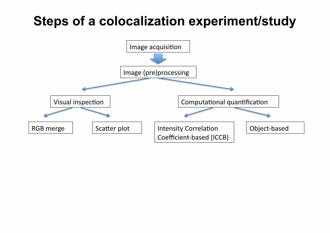
Steps of a colocalization experiment/study

Image  acquisi,on  

Image  (pre)processing  

Visual  inspec,on   Computa,onal  quan,fica,on  

RGB  merge   Sca<er  plot   Intensity  Correla,on  Coefficient-­‐based  (ICCB)  

Object-­‐based  

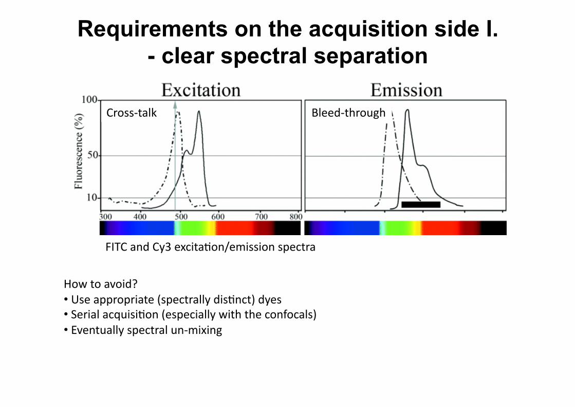
Requirements on the acquisition side I. - clear spectral separation

FITC  and  Cy3  excita,on/emission  spectra  

Cross-­‐talk   Bleed-­‐through  

How  to  avoid?  •   Use  appropriate  (spectrally  dis,nct)  dyes  •   Serial  acquisi,on  (especially  with  the  confocals)  •   Eventually  spectral  un-­‐mixing  

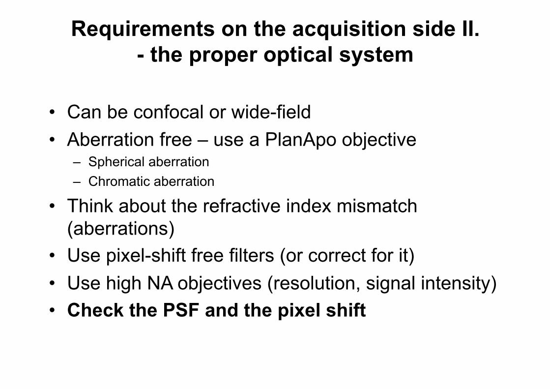
Requirements on the acquisition side II. - the proper optical system

•  Can be confocal or wide-field •  Aberration free – use a PlanApo objective

–  Spherical aberration –  Chromatic aberration

•  Think about the refractive index mismatch (aberrations)

•  Use pixel-shift free filters (or correct for it) •  Use high NA objectives (resolution, signal intensity) •  Check the PSF and the pixel shift

Requirements on the acquisition side III. - setting up the detector

•  Important to have Nyquist (2-3x oversampling) but don’t overdo it

•  The noise (S/N ratio of the image) is critical so scan slowly/average (confocal), integrate long (wide-field)

•  Use the whole dynamic range (no saturation), see that the two channels match to each-other

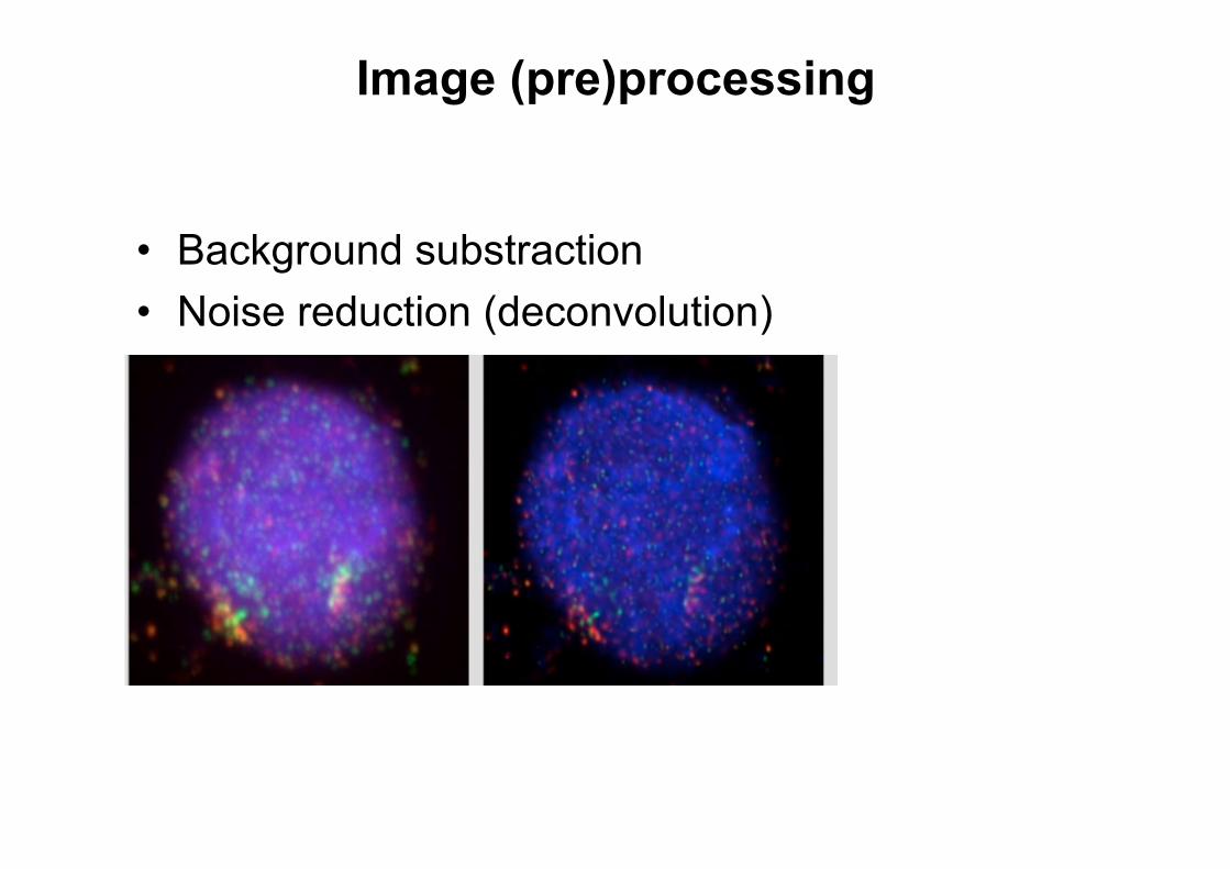
Image (pre)processing

•  Background substraction •  Noise reduction (deconvolution)

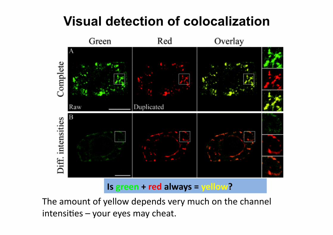
Visual detection of colocalization

Is  green  +  red  always  =  yellow?  

The  amount  of  yellow  depends  very  much  on  the  channel  intensi,es  –  your  eyes  may  cheat.  

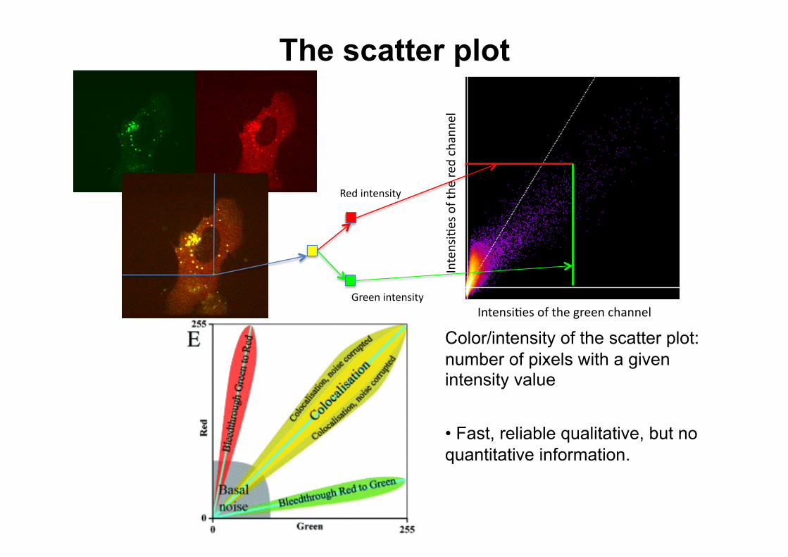
The scatter plot

Intensi,es  of  the  green  channel  

Intensi,es  of  the

 red  channe

l  

Red  intensity  

Green  intensity  

Color/intensity of the scatter plot: number of pixels with a given intensity value

•  Fast, reliable qualitative, but no quantitative information.

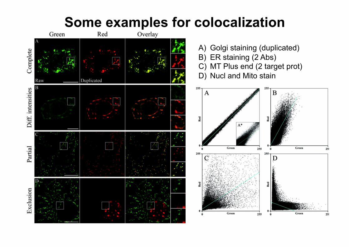
Some examples for colocalization A)  Golgi staining (duplicated) B)  ER staining (2 Abs) C)  MT Plus end (2 target prot) D)  Nucl and Mito stain

Intensity correlation coefficient based methods

•  Many possible parameters (e.g. Pearson’s) •  The choice (best one) is image/application/question

dependent – no general rules •  All methods can be calculated for the whole image or for

a ROI •  Way of calculation may differ between software (e.g. including 0 value pixels or not in the average

calculation) •  Tresholded parameters (manual or automated) •  Most software packages calculate all of them

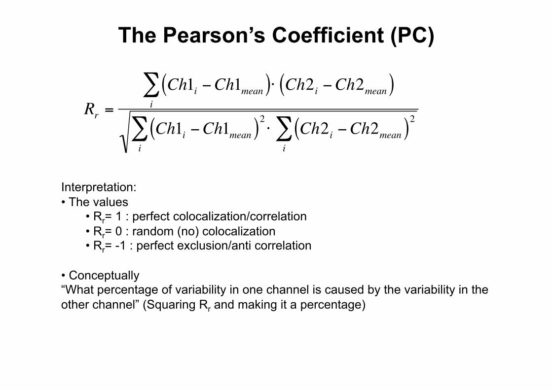
The Pearson’s Coefficient (PC)

€

Rr =

Ch1i −Ch1mean( )⋅ Ch2i −Ch2mean( )i∑

Ch1i −Ch1mean( )2 ⋅ Ch2i −Ch2mean( )2i∑

i∑

Interpretation: •  The values

•  Rr= 1 : perfect colocalization/correlation •  Rr= 0 : random (no) colocalization •  Rr= -1 : perfect exclusion/anti correlation

•  Conceptually “What percentage of variability in one channel is caused by the variability in the other channel” (Squaring Rr and making it a percentage)

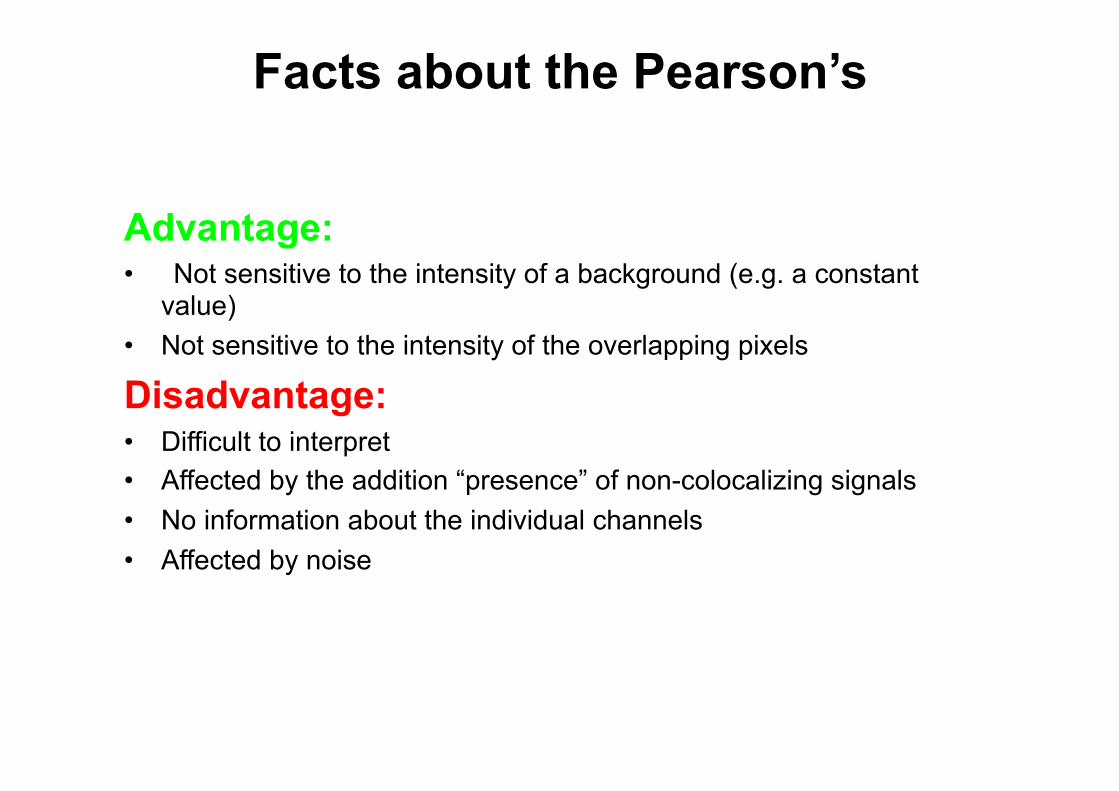
Facts about the Pearson’s

Advantage: •  Not sensitive to the intensity of a background (e.g. a constant

value) •  Not sensitive to the intensity of the overlapping pixels

Disadvantage: •  Difficult to interpret •  Affected by the addition “presence” of non-colocalizing signals •  No information about the individual channels •  Affected by noise

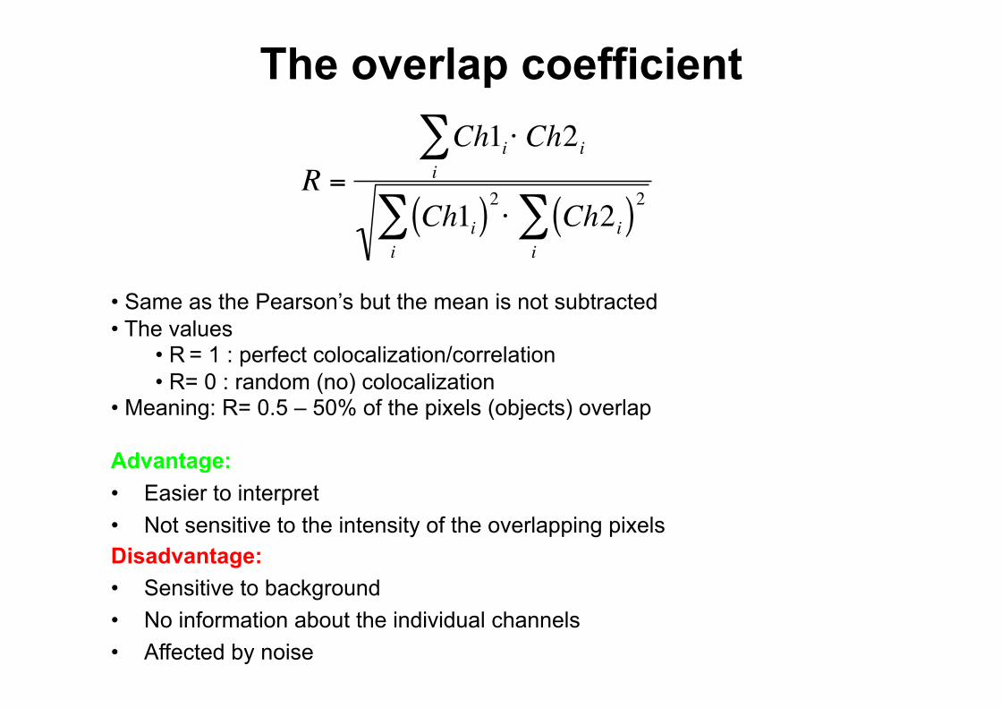
The overlap coefficient

€

R =

Ch1i ⋅ Ch2ii∑

Ch1i( )2 ⋅ Ch2i( )2i∑

i∑

•  Same as the Pearson’s but the mean is not subtracted •  The values

•  R = 1 : perfect colocalization/correlation •  R= 0 : random (no) colocalization

•  Meaning: R= 0.5 – 50% of the pixels (objects) overlap

Advantage: •  Easier to interpret •  Not sensitive to the intensity of the overlapping pixels Disadvantage: •  Sensitive to background •  No information about the individual channels •  Affected by noise

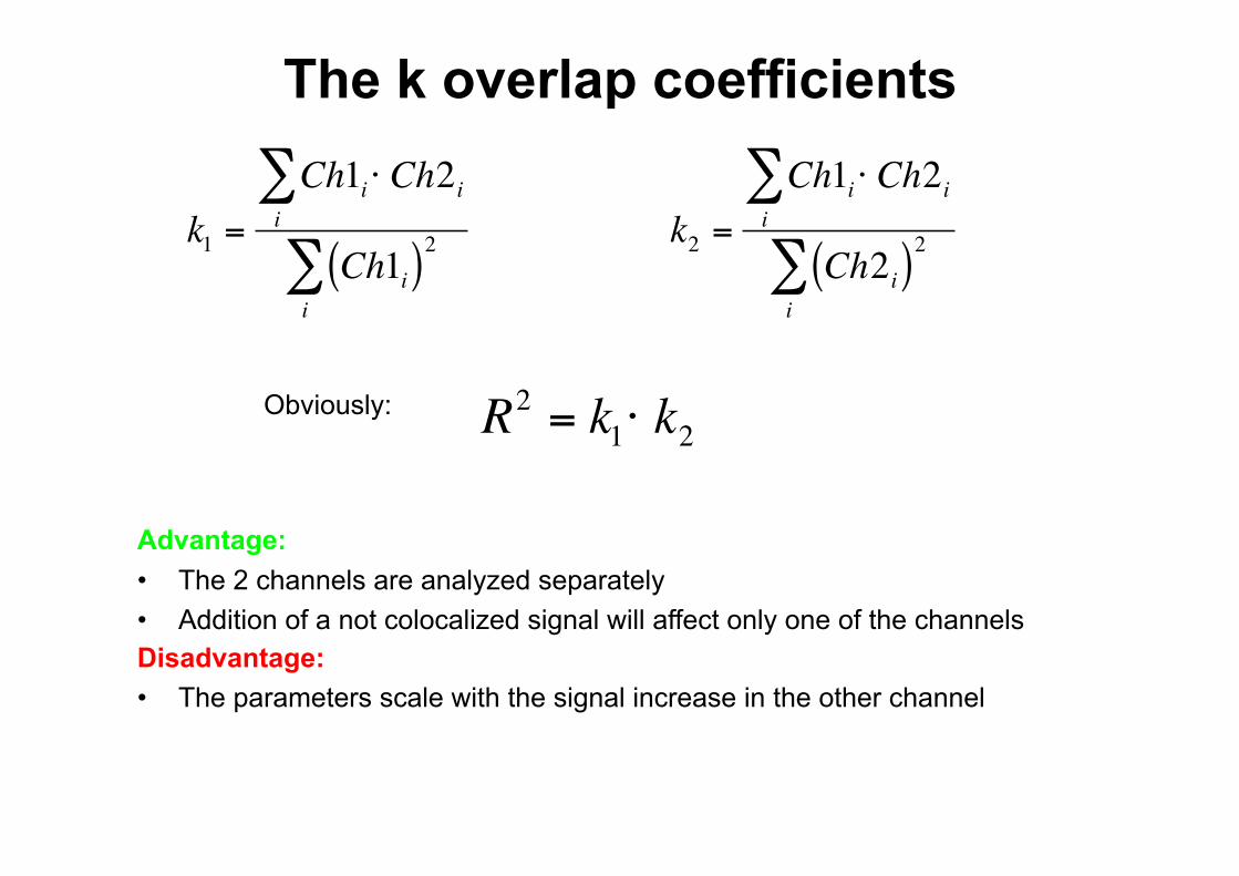
The k overlap coefficients

€

k1 =

Ch1i ⋅ Ch2ii∑

Ch1i( )2i∑

€

k2 =

Ch1i ⋅ Ch2ii∑

Ch2i( )2i∑

Advantage: •  The 2 channels are analyzed separately •  Addition of a not colocalized signal will affect only one of the channels Disadvantage: •  The parameters scale with the signal increase in the other channel

Obviously:

€

R2 = k1⋅ k2

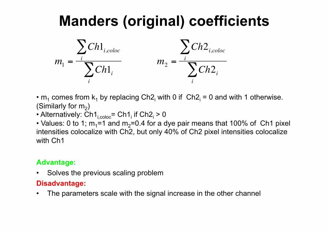
Manders (original) coefficients

€

m1 =

Ch1i,coloci∑

Ch1ii∑

€

m2 =

Ch2i,coloci∑

Ch2ii∑

•  m1 comes from k1 by replacing Ch2i with 0 if Ch2i = 0 and with 1 otherwise. (Similarly for m2) •  Alternatively: Ch1i,coloc= Ch1i if Ch2i > 0 •  Values: 0 to 1; m1=1 and m2=0.4 for a dye pair means that 100% of Ch1 pixel intensities colocalize with Ch2, but only 40% of Ch2 pixel intensities colocalize with Ch1

Advantage: •  Solves the previous scaling problem Disadvantage: •  The parameters scale with the signal increase in the other channel

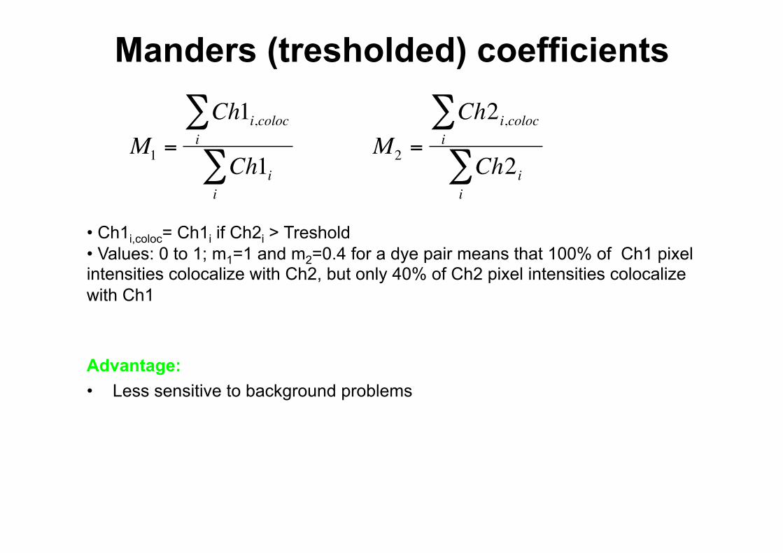
Manders (tresholded) coefficients

€

M1 =

Ch1i,coloci∑

Ch1ii∑

€

M2 =

Ch2i,coloci∑

Ch2ii∑

•  Ch1i,coloc= Ch1i if Ch2i > Treshold •  Values: 0 to 1; m1=1 and m2=0.4 for a dye pair means that 100% of Ch1 pixel intensities colocalize with Ch2, but only 40% of Ch2 pixel intensities colocalize with Ch1

Advantage: •  Less sensitive to background problems

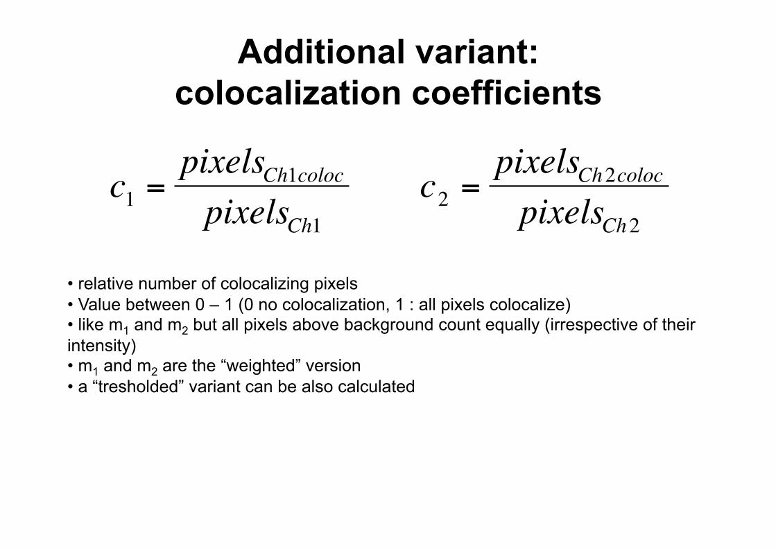
Additional variant: colocalization coefficients

€

c1 =pixelsCh1colocpixelsCh1

€

c2 =pixelsCh2colocpixelsCh2

•  relative number of colocalizing pixels •  Value between 0 – 1 (0 no colocalization, 1 : all pixels colocalize) •  like m1 and m2 but all pixels above background count equally (irrespective of their intensity) •  m1 and m2 are the “weighted” version •  a “tresholded” variant can be also calculated

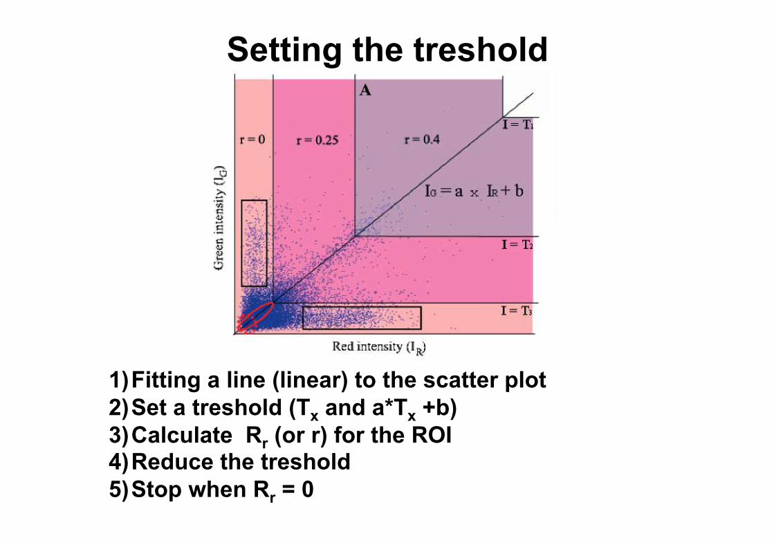
Setting the treshold

1) Fitting a line (linear) to the scatter plot 2) Set a treshold (Tx and a*Tx +b) 3) Calculate Rr (or r) for the ROI 4) Reduce the treshold 5) Stop when Rr = 0

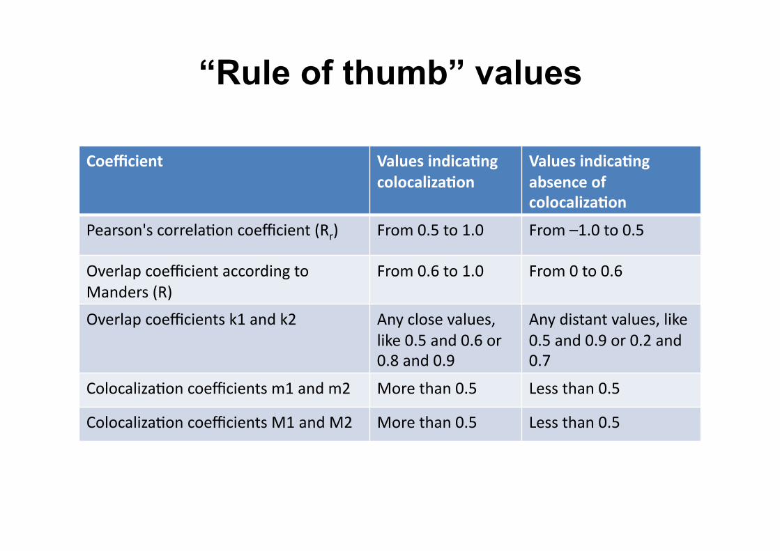
“Rule of thumb” values

Coefficient     Values  indica8ng  colocaliza8on  

Values  indica8ng  absence  of  colocaliza8on  

Pearson's  correla,on  coefficient  (Rr)   From  0.5  to  1.0   From  –1.0  to  0.5  

Overlap  coefficient  according  to  Manders  (R)    

From  0.6  to  1.0   From  0  to  0.6  

Overlap  coefficients  k1  and  k2   Any  close  values,  like  0.5  and  0.6  or  0.8  and  0.9  

Any  distant  values,  like  0.5  and  0.9  or  0.2  and  0.7  

Colocaliza,on  coefficients  m1  and  m2     More  than  0.5   Less  than  0.5  

Colocaliza,on  coefficients  M1  and  M2     More  than  0.5   Less  than  0.5  

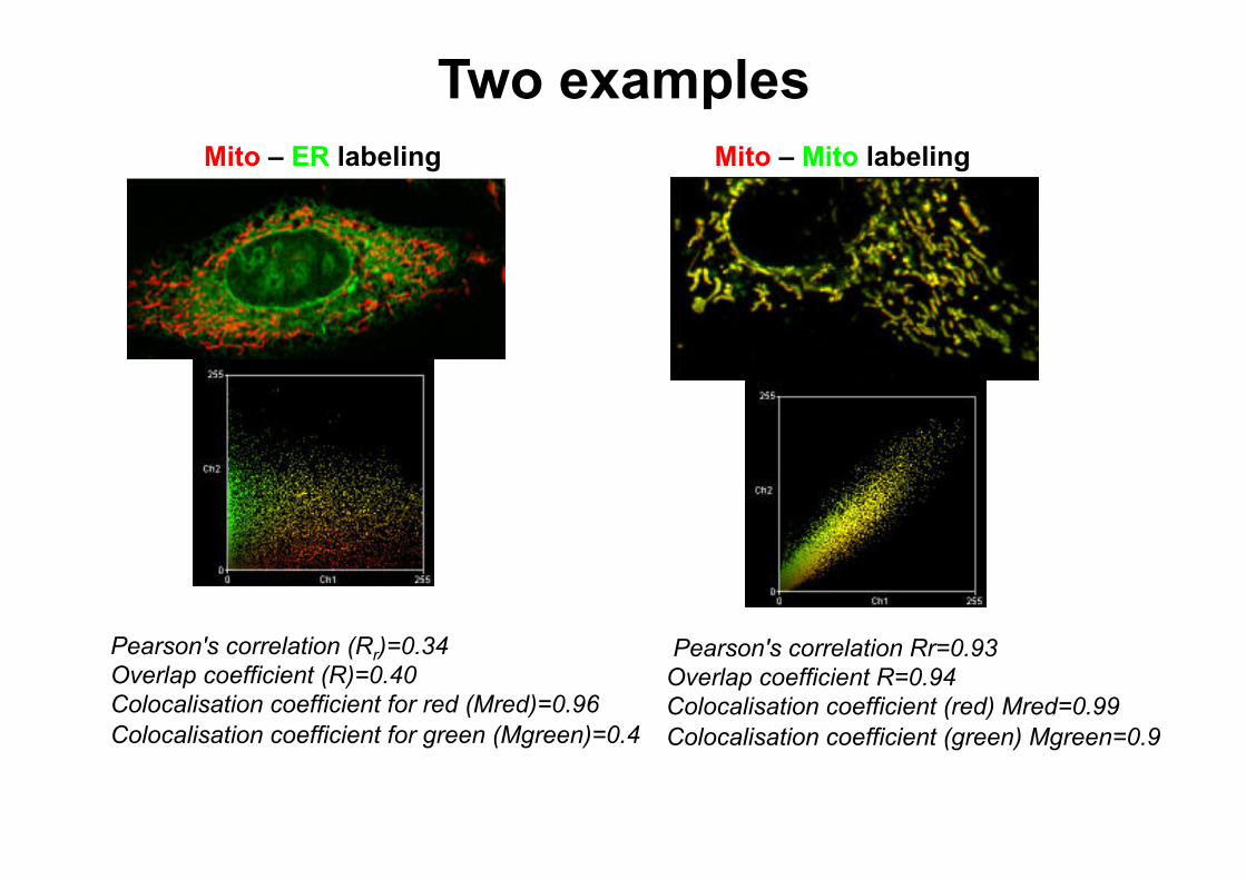
Two examples Mito – ER labeling

Pearson's correlation (Rr)=0.34 Overlap coefficient (R)=0.40 Colocalisation coefficient for red (Mred)=0.96 Colocalisation coefficient for green (Mgreen)=0.4

Pearson's correlation Rr=0.93 Overlap coefficient R=0.94 Colocalisation coefficient (red) Mred=0.99 Colocalisation coefficient (green) Mgreen=0.9

Mito – Mito labeling

Relevance (statistical significance) of the measured parameters

•  Image randomization (Costes) - The Ch1 image is compared to 200 “scrambled” Ch2 images - Scrambling: randomly rearranging the blocks (size equals to the PSF) of Ch2

•  Image translation –  X direction (Van Steensel) –  X-Y and Z direction (Fay)

•  In all cases the parameter (coloc) is significant if greater the 95% of the randomized images

Object based methods

0. Line profile (for small objects) 1.  Segmentation 2.  Determining the colocalization

–  Colocalized (overlapping) volume –  Colocalized (overlapping) area –  Centroid distance

Advantage: •  Less dependent on intensities (diffuse labeling) •  Can be automated

Disadvantage: •  Segmentation needed (difficult) •  Doesn’t work for diffuse labeling

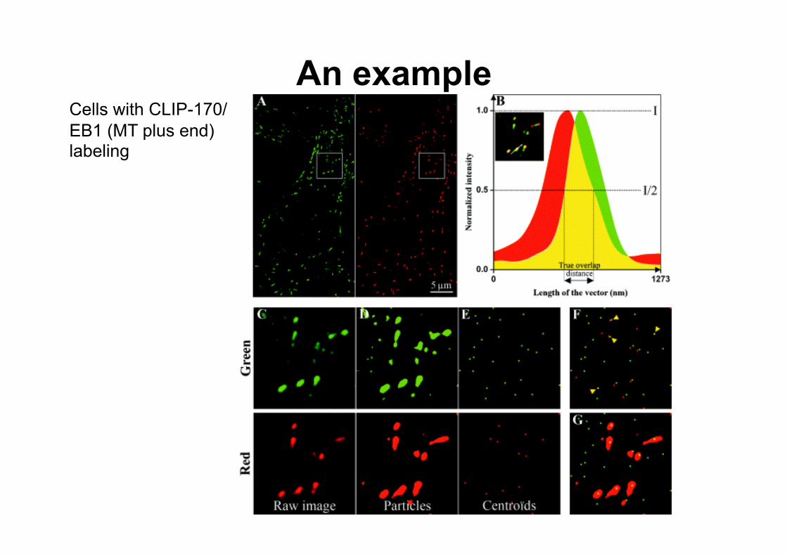
An example Cells with CLIP-170/EB1 (MT plus end) labeling

Links •  The JACop plugin: http://imagejdocu.tudor.ludoku.phpid=plugin:analysis:jacop_2.0:just_another_colocalization_plugin:start

•  The Olympus interactive tutorial: http://www.olympusfluoview.com/java/colocalization/index.html

•  An ImageJ based tutorial: http://www.med.unc.edu/microscopy/resources/learning/colocalization-tutorial/Colocalization%20Overview/

•  The Fiji colocalization analysis http://pacific.mpi-cbg.de/wiki/index.php/Colocalization_Analysis

•  A PerkinElmer video tutorial http://www.cellularimaging.com/tutorials/colocalization/

And others…..