Quantitative Colocalization Analysis of Confocal Fluorescence

UNIT 4.19Quantitative Colocalization Analysis ofConfocal Fluorescence MicroscopyImages

Vadim Zinchuk1 and Olga Zinchuk2

1Department of Anatomy and Cell Biology, Kochi University, Faculty of Medicine, Japan2Institute of Anatomy, University of Berne, CH-3000, Berne, Switzerland

ABSTRACT

Colocalization is an important finding in many cell biological studies. This unit describesa protocol for quantitative evaluation of images with colocalization based on the calcula-tion of a number of specialized coefficients. First, images of double-stained sections aresubjected to background correction. Then, various coefficients are calculated. Meaningsof the coefficients and a guide to interpretation of their results indicating either pres-ence or absence of colocalization are given. Success in colocalization studies dependson the quality of analyzed images, proper preparation of them for coefficients calcu-lations, and correct interpretation of obtained results. This protocol helps to ensurereliability of colocalization coefficients calculations. Curr. Protoc. Cell Biol. 39:4.19.1-4.19.16. C© 2008 by John Wiley & Sons, Inc.

Keywords: quantitative colocalization � confocal fluorescence microscopy �

image analysis

INTRODUCTION

Quantitative colocalization analysis (QCA) is a method to estimate the degree of colo-calization of antigens in multicolor confocal immunofluorescence microscopy images.Colocalization is observed when staining of two or more antigens in the same section,labeled by corresponding antibodies with different excitation spectra and therefore vi-sualized in different colors, overlaps. Although colocalization is a mere coexistence ofmolecules in a very close physical location, it can provide valuable clues clarifyingtheir common characteristics. Scientific applicability of colocalization observed per seis, however, limited because it is perceived differently by the eye and thus can frequentlybe misleading. Thus, the method described here evaluates colocalization objectively byestimating its quantitative characteristics.

The method is applicable to dual-color confocal images of sections stained with anti-bodies with well-separated excitation spectra, acquired using proper set up of confocalmicroscopes, and stored in the image file format that preserves image data necessaryfor quantification. It relies on the use of specialized software that calculates a numberof colocalization coefficients to understand the observed colocalization in greater detail.Prior to calculating the coefficients, the software performs background correction of theimages. This important step is required to avoid obtaining false-positive results and isnot available with other tools.

The protocol described in this unit demonstrates the use of QCA for studying functionallysynergetic proteins. As an example, the use of the method is illustrated by quantifyingcolocalization of bile salt export pump (Bsep) and multidrug resistance protein 2 (Mrp2)in the liver. The background correction procedure is performed using different methodsand is accompanied by the respective scatter grams. The meanings of coefficients and

Current Protocols in Cell Biology 4.19.1-4.19.16, June 2008Published online June 2008 in Wiley Interscience (www.interscience.wiley.com).DOI: 10.1002/0471143030.cb0419s39Copyright C© 2008 John Wiley & Sons, Inc.

Microscopy

4.19.1

Supplement 39

mamunoz

Subrayado

QuantitativeColocalization

Analysis ofConfocal

FluorescentMicroscopy

Images

4.19.2

Supplement 39 Current Protocols in Cell Biology

their importance is explained. Finally, the interpretation of the results of coefficientscalculations in terms of their biological significance is given.

STRATEGIC PLANNING

General

Successful QCA requires good knowledge and experience in basic immunohistochemi-cal techniques (UNIT 4.3), confocal fluorescence microscopy (UNIT 4.5), and handling andprocessing of digital images. This unit provides practical information about quantitativecolocalization and coefficients used to estimate it, gives tips for success in backgroundcorrection procedure, and describes applicability of calculations results. Please refer toUNITS 4.2 and 4.3 for basic information on basic fluorescence microscopy and immunoflu-orescence staining, respectively.

Steps of QCA

1. Ensure that image is properly prepared, acquired, and processed.

2. Open image in colocalization analysis software and perform background correction.

3. Calculate colocalization coefficients.

4. Save obtained results for further reference.

See also Table 4.19.1 for comments and tips.

Importance of Using Properly Prepared Images

Although QCA is the most important step in colocalization studies, it is just the final step.Its results are fully dependent on all previous steps of sample preparation, microscope setup, and image acquisition and handling. To emphasize the importance of image suitabilityto ensure reliable results of coefficients calculations, it is presented as a first step of QCA.The most important rules which should be followed to obtain confocal images useablefor quantification are as follows:

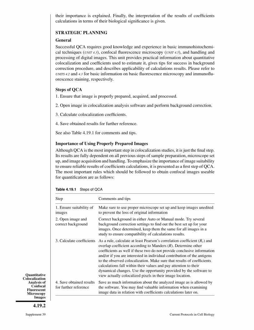
Table 4.19.1 Steps of QCA

Step Comments and tips

1. Ensure suitability ofimages

Make sure to use proper microscope set up and keep images uneditedto prevent the loss of original information

2. Open image andcorrect background

Correct background in either Auto or Manual mode. Try severalbackground correction settings to find out the best set up for yourimages. Once determined, keep them the same for all images in astudy to ensure compatibility of calculations results.

3. Calculate coefficients As a rule, calculate at least Pearson’s correlation coefficient (Rr) andoverlap coefficient according to Manders (R). Determine othercoefficients as well if these two do not provide conclusive informationand/or if you are interested in individual contribution of the antigensto the observed colocalization. Make sure that results of coefficientscalculations fall within their values and pay attention to theirdynamical changes. Use the opportunity provided by the software toview actually colocalized pixels in their image location.

4. Save obtained resultsfor further reference

Save as much information about the analyzed image as is allowed bythe software. You may find valuable information when examiningimage data in relation with coefficients calculations later on.

Microscopy

4.19.3

Current Protocols in Cell Biology Supplement 39

Sample preparation1. Ensure that the antibodies you are using are specific and do not cross react.

2. Make the proper choice of fluorophores by selecting ones with well-separated excita-tion and emission spectra.

3. Use the same mounting medium for all of the samples that you will be performingcalculations on.

4. As antifading reagents tend to increase background fluorescence, try to avoid usingthem.

5. Always use unstained control samples to check for autofluorescence.

Microscope set up1. Reduce chromatic shift by using plan apochromatic lenses.

2. Maximize emission collection while avoiding bleed-through effect by using optimizedemission filters.

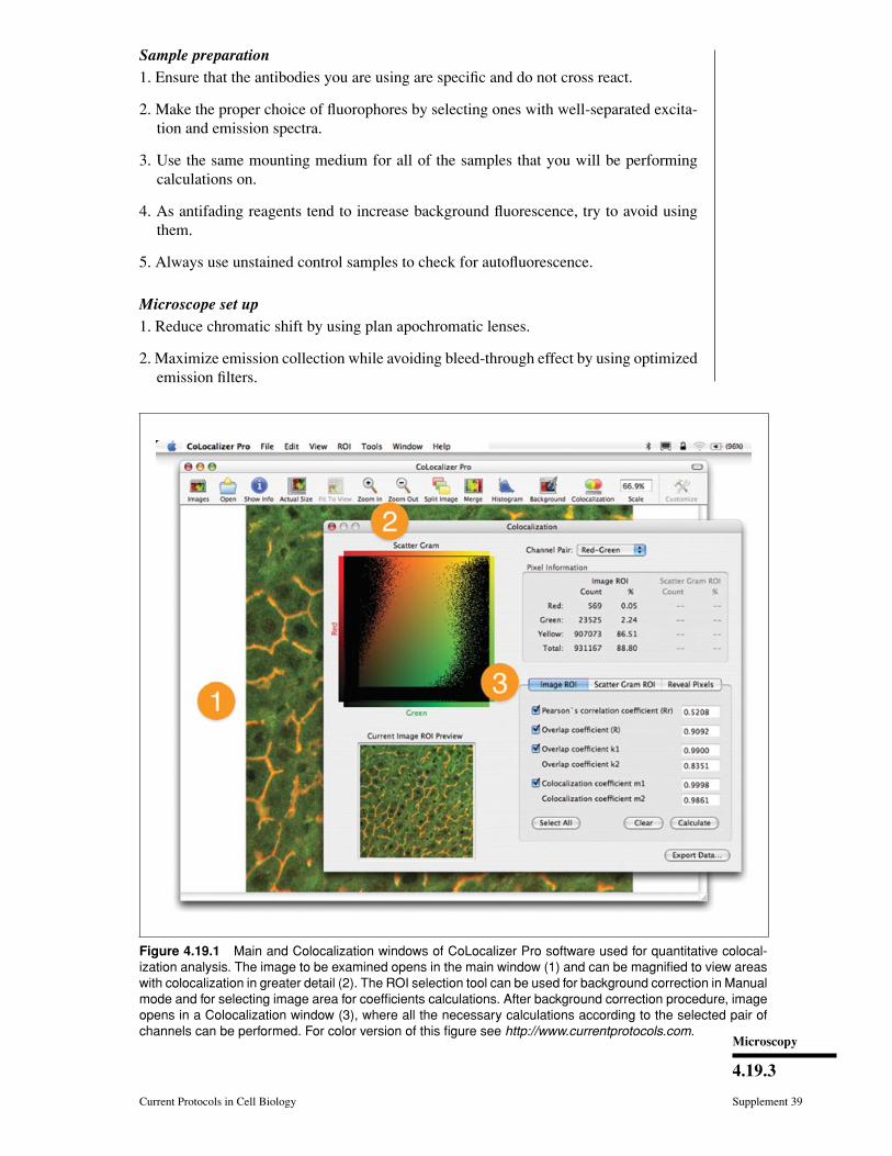
Figure 4.19.1 Main and Colocalization windows of CoLocalizer Pro software used for quantitative colocal-ization analysis. The image to be examined opens in the main window (1) and can be magnified to view areaswith colocalization in greater detail (2). The ROI selection tool can be used for background correction in Manualmode and for selecting image area for coefficients calculations. After background correction procedure, imageopens in a Colocalization window (3), where all the necessary calculations according to the selected pair ofchannels can be performed. For color version of this figure see http://www.currentprotocols.com.

4.19.4


3. Make sure you are using the same objective lens for obtaining all images you areplanning to compare.

4. Ensure proper set up of the size of microscope pinhole.

Image acquisition and handling1. Remember to acquire images sequentially to minimize bleed-through effect.

2. Avoid acquiring images that are too bright and images with too much contrast, as itmay result in image saturation.

3. Never resave image files in any other graphic format than TIFF, as it may result in theloss of original data necessary for quantification.

4. Remember that any adjustments of brightness, contrast, etc. of your images usinggraphics-editing software may prevent further use of them for quantification purposes.

5. After making sure your images are suitable for colocalization studies, open them inQCA software (Fig. 4.19.1) and perform quantitative analysis according to the protocolbelow.

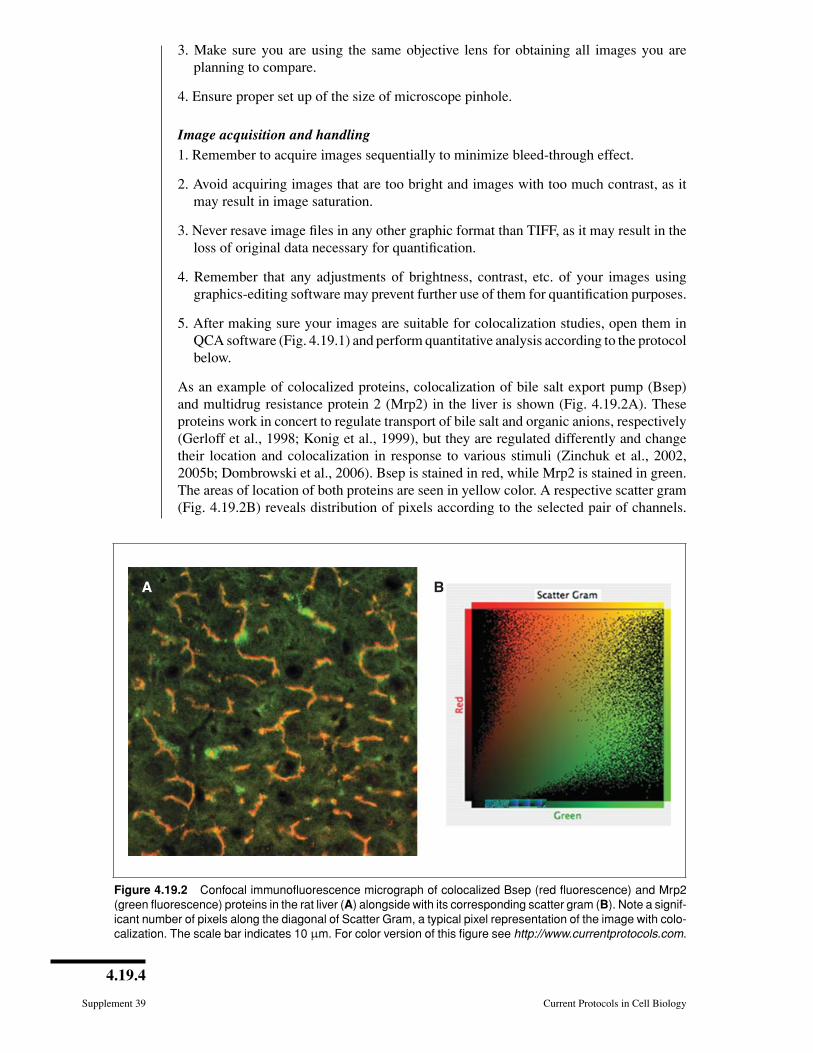
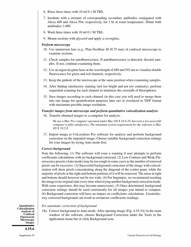
As an example of colocalized proteins, colocalization of bile salt export pump (Bsep)and multidrug resistance protein 2 (Mrp2) in the liver is shown (Fig. 4.19.2A). Theseproteins work in concert to regulate transport of bile salt and organic anions, respectively(Gerloff et al., 1998; Konig et al., 1999), but they are regulated differently and changetheir location and colocalization in response to various stimuli (Zinchuk et al., 2002,2005b; Dombrowski et al., 2006). Bsep is stained in red, while Mrp2 is stained in green.The areas of location of both proteins are seen in yellow color. A respective scatter gram(Fig. 4.19.2B) reveals distribution of pixels according to the selected pair of channels.

A B

Figure 4.19.2 Confocal immunofluorescence micrograph of colocalized Bsep (red fluorescence) and Mrp2(green fluorescence) proteins in the rat liver (A) alongside with its corresponding scatter gram (B). Note a signif-icant number of pixels along the diagonal of Scatter Gram, a typical pixel representation of the image with colo-calization. The scale bar indicates 10 μm. For color version of this figure see http://www.currentprotocols.com.

Microscopy

4.19.5


In the scatter gram, colocalized pixels are located along the diagonal, while those withno colocalization occupy left and bottom portions. As can be seen in the figure, thescatter gram represents unique information about an image file and is useful for viewingcolocalized pixels in the image.

BASICPROTOCOL

QUANTIATIVE COLOCALIZATION ANALYSIS

The present protocol is used to quantify colocalization in dual-color confocal microscopyimages of sections stained with fluorescence-labeled antibodies with well-separated ex-citation spectra, obtained using correct microscope set up, and saved in the image fileformat that ensures preservation of image data required for quantification. It relies onthe use of specialized software that enables determination of colocalization coefficientswithin a single session of image analysis, making calculation results not only highlyrelevant and comparable, but also easily reproducible. The validation of the results ofquantitative colocalization experiments and their applicability are presented.

Materials

Cryostat-cut 6- to 8-μm thick sections of rat liverAcetone for tissue fixationBlocking solution: 10% (v/v) goat serum in 0.1 M Tris-buffered saline (TBS)

containing 0.1% Triton X-100Primary antibodies against Bsep and Mrp2 proteins [Santa Cruz Biotechnology;

anti-Bsep antibody was donated by Dr. Bruno Stieger (Department of Medicine,University of Zurich, Switzerland)] or other proteins of interest (primaryantibodies should be raised in different species)

Non-immune IgG to control the specificity of immunostaining0.1 M Tris-buffered saline (TBS; APPENDIX 2A)Corresponding secondary antibodies with different excitation spectra, e.g., Alexa

488 and Alexa 594 from Molecular Probes (antibodies should not becross-reacting)

Glycerol

Poly-L-lysine-coated glass slidesCover glass for mounting sectionsConfocal microscope for image acquisition (any brand)Argon-krypton laser (Siemens)Software: either CoLocalizer Pro or CoLocalizer Express (CoLocalization

Research Software; http://homepage.mac.com/colocalizerpro/) for QCA

Additional reagents and equipment for immunofluorescence staining (UNIT 4.3) andfluorescence microscopy (UNIT 4.2)

Perform immunostaining1. Pick up a 6- to 8-μm thick section of liver on poly-L-lysine-coated glass slides, air

dry for 1 hr, and fix in acetone for 30 min at −20◦C.

2. Apply 500 μl blocking solution for 1 hr at room temperature to block nonspecificbinding.

3. Incubate with 500 μl anti-Bsep antibody diluted 1:100 for 1 hr at room temperature.

In parallel, perform the same procedure using non-immune IgG instead of primary anti-bodies to control specificity of immunostaining.

4. Rinse three times with 10 ml of 0.1 M TBS.

5. Incubate with 500 μl anti-Mrp2 antibody diluted 1:100 for another 1 hour at roomtemperature.


Analysis ofConfocal


Images

4.19.6


6. Rinse three times with 10 ml 0.1 M TBS.

7. Incubate with a mixture of corresponding secondary antibodies conjugated withAlexa 488 and Alexa 594, respectively, for 1 hr at room temperature. Dilute bothantibodies 1:400.

8. Wash three times with 10 ml 0.1 M TBS.

9. Mount sections with glycerol and apply a coverglass.

Perform microscopy10. Use immersion lens (e.g., Plan-Neofluar 40 /0.75 mm) of confocal microscope to

examine sections.

11. Check samples for autofluorescence. If autofluorescence is detected, discard sam-ples. If not, continue examining them.

12. Use an argon-krypton laser at the wavelength of 488 and 543 nm to visualize doublefluorescence for green and red channels, respectively.

13. Keep the pinhole of the microscope at the same position when examining samples.

14. After finding satisfactory staining (not too bright and not too contrasty), performsequential scanning for each channel to minimize the crosstalk of fluorophores.

15. Save images according to each channel (in this case you will need to merge theminto one image for quantification purposes later on) or overlayed in TIFF formatwith maximum possible image resolution.

Transfer images from microscope and perform quantitative colocalization analysis16. Transfer obtained images to a computer for analysis.

We use a Mac Pro computer operated under Mac OS X 10.4.10, but even a less powerfulcomputer is fully satisfactory. The minimum system requirement for the software is MacOS X 10.2.8.

17. Import image to CoLocalizer Pro software for analysis and perform backgroundcorrection on the imported image. Choose suitable background correction settingsfor your images by trying Auto mode first.

Correct backgroundNote the following: (1) The software will issue a warning if user attempts to performcoefficients calculations with no background corrected. (2) Low Contrast and Weak Flu-orescence presets (Auto mode) may be too rough in some cases as the number of removedpixels can be excessive. (3) Successful background correction of the image with colocal-ization will show pixels concentrating along the diagonal of the scatter gram, while themajority of pixels at the right and bottom portions of it will be removed. The areas at rightand bottom should however not be too wide. (4) For beginners, we recommend resettingthe image to its original state every time when trying another background correction mode.With some experience, this may become unnecessary. (5) Once determined, backgroundcorrection settings should be used consistently for all images you intend to compare.(6) Background correction will have an impact on coefficients calculations. Unsatisfac-tory corrected background can result in erroneous coefficients readings.

For automatic correction of background

18a. Correct background in Auto mode. After opening image (Fig. 4.19.3A) in the mainwindow of the software, choose Background Correction under the Tools in theapplication menu bar or click Background icon.

Microscopy

4.19.7


A

C

B

D

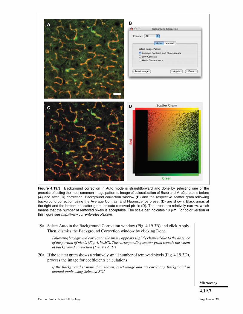
Figure 4.19.3 Background correction in Auto mode is straightforward and done by selecting one of thepresets reflecting the most common image patterns. Image of colocalization of Bsep and Mrp2 proteins before(A) and after (C) correction. Background correction window (B) and the respective scatter gram followingbackground correction using the Average Contrast and Fluorescence preset (D) are shown. Black areas atthe right and the bottom of scatter gram indicate removed pixels (D). The areas are relatively narrow, whichmeans that the number of removed pixels is acceptable. The scale bar indicates 10 μm. For color version ofthis figure see http://www.currentprotocols.com.

19a. Select Auto in the Background Correction window (Fig. 4.19.3B) and click Apply.Then, dismiss the Background Correction window by clicking Done.

Following background correction the image appears slightly changed due to the absenceof the portion of pixels (Fig. 4.19.3C). The corresponding scatter gram reveals the extentof background correction (Fig. 4.19.3D).

20a. If the scatter gram shows a relatively small number of removed pixels (Fig. 4.19.3D),process the image for coefficients calculations.

If the background is more than shown, reset image and try correcting background inmanual mode using Selected ROI.


Analysis ofConfocal


Images

4.19.8


A

C

B

D

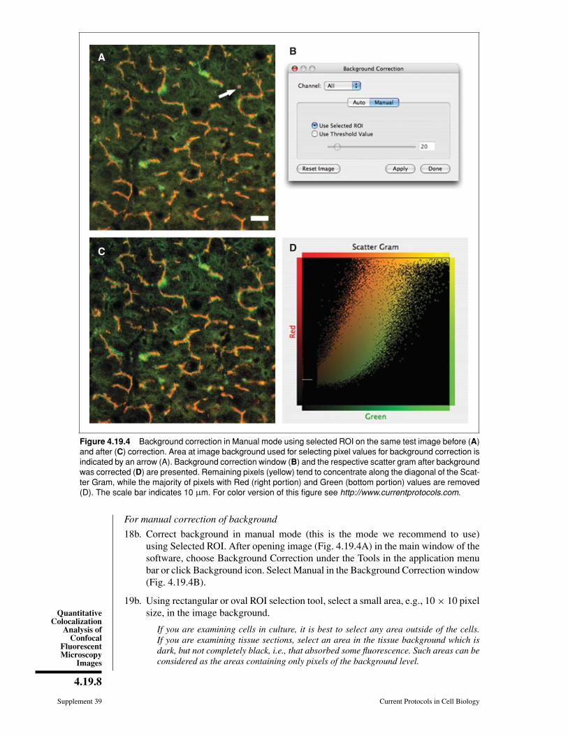
Figure 4.19.4 Background correction in Manual mode using selected ROI on the same test image before (A)and after (C) correction. Area at image background used for selecting pixel values for background correction isindicated by an arrow (A). Background correction window (B) and the respective scatter gram after backgroundwas corrected (D) are presented. Remaining pixels (yellow) tend to concentrate along the diagonal of the Scat-ter Gram, while the majority of pixels with Red (right portion) and Green (bottom portion) values are removed(D). The scale bar indicates 10 μm. For color version of this figure see http://www.currentprotocols.com.

For manual correction of background

18b. Correct background in manual mode (this is the mode we recommend to use)using Selected ROI. After opening image (Fig. 4.19.4A) in the main window of thesoftware, choose Background Correction under the Tools in the application menubar or click Background icon. Select Manual in the Background Correction window(Fig. 4.19.4B).

19b. Using rectangular or oval ROI selection tool, select a small area, e.g., 10 × 10 pixelsize, in the image background.

If you are examining cells in culture, it is best to select any area outside of the cells.If you are examining tissue sections, select an area in the tissue background which isdark, but not completely black, i.e., that absorbed some fluorescence. Such areas can beconsidered as the areas containing only pixels of the background level.

Microscopy

4.19.9


20b. Then, click Apply and dismiss Background Correction window by clicking Done.

Following background correction the image will appear changed depending on thenumber of removed pixels (Fig. 4.19.4C). The corresponding scatter gram reveals theextent of background correction (Fig. 4.19.4D). Figure 4.19.4D shows what the scattergram of a properly corrected image should look like: remaining pixels concentratemainly along the diagonal of the scatter gram and the areas of removed red (at right)and green (at left) pixels are not too wide.

You may also try correcting background in Manual mode using Threshold Value. Wefind it useful for images that are more bright and contrasty than the average. It workssimilarly to Auto mode, with the exception that you are free to choose the exact numberof pixels to be removed. It can provide good correction results, but, in comparison tothe selected ROI option, does not give the important advantage of being able to tailorcorrection to the unique pixel profile of analyzed images.

21. After background correction step, perform coefficients calculations.

Calculate coefficients and view colocalized pixels22. Using the whole image as a ROI, open Colocalization window, and proceed as

described below.

23. Depending on the shape appearance of areas with colocalization, use a suitable ROItool in the menu bar to select image areas containing predominantly colocalization.

In the test image used in this protocol, we used the Lasso tool.

24. Repeat calculations for at least three different areas with colocalization.

Thus, you will have at least four sets of data: one for the whole image and the otherthree for each of the selected ROIs. The resulting coefficients values will be the averageof these four.

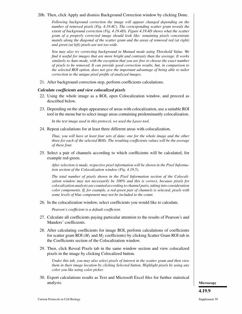
25. Select a pair of channels according to which coefficients will be calculated, forexample red-green.

After selection is made, respective pixel information will be shown in the Pixel Informa-tion section of the Colocalization window (Fig. 4.19.5).

The total number of pixels shown in the Pixel Information section of the Colocali-zation window may not necessarily be 100% and this is correct, because pixels forcolocalization analysis are counted according to channel pairs, taking into considerationcolor components. If, for example, a red-green pair of channels is selected, pixels withsome levels of blue component may not be included to the count.

26. In the colocalization window, select coefficients you would like to calculate.

Pearson’s coefficient is a default coefficient.

27. Calculate all coefficients paying particular attention to the results of Pearson’s andManders’ coefficients.

28. After calculating coefficients for image ROI, perform calculations of coefficientsfor scatter gram ROI (M1 and M2 coefficients) by clicking Scatter Gram ROI tab inthe Coefficients section of the Colocalization window.

29. Then, click Reveal Pixels tab in the same window section and view colocalizedpixels in the image by clicking Colocalized button.

Under this tab, you may also select pixels of interest in the scatter gram and then viewthem in their image location by clicking Selected button. Highlight pixels by using anycolor you like using color picker.

30. Export calculations results as Text and Microsoft Excel files for further statisticalanalysis.


Analysis ofConfocal


Images

4.19.10


Figure 4.19.5 Colocalization window of the software shows scatter gram (1) of the selected ROI,the ROI itself (2), a pair of channels according to which the coefficients can be calculated (3), pixelinformation of the analyzed ROI (4), and the options to perform calculations of the coefficients(5). The important option to view exclusively colocalized pixels in the image is also given (6). Allcalculations results can be exported as Text and Microsoft Excel files. All data used for calculationscan be saved in PDF and HTML formats and presented as session reports. For color version ofthis figure see http://www.currentprotocols.com.

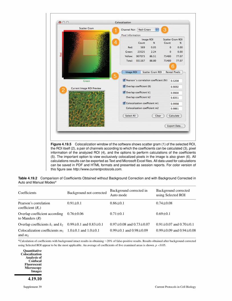
Table 4.19.2 Comparison of Coefficients Obtained without Background Correction and with Background Corrected inAuto and Manual Modesa

Coefficients Background not correctedBackground corrected inAuto mode

Background correctedusing Selected ROI

Pearson’s correlationcoefficient (Rr)

0.91±0.1 0.86±0.1 0.74±0.08

Overlap coefficient accordingto Manders (R)

0.76±0.06 0.71±0.1 0.69±0.1

Overlap coefficients k1 and k2 0.99±0.1 and 0.83±0.1 0.97±0.08 and 0.73±0.07 0.91±0.07 and 0.70±0.1

Colocalization coefficients m1

and m2

1.0±0.1 and 1.0±0.1 0.99±0.1 and 0.98±0.09 0.99±0.09 and 0.94±0.08

aCalculation of coefficients with background intact results in obtaining ∼20% of false-positive results. Results obtained after background correctedusing Selected ROI appear to be the most applicable. An average of coefficients of five examined areas is shown. p <0.05.

Microscopy

4.19.11


31. Make a report of the calculations session in either PDF or HTML format.

In addition to the analyzed image and calculations results, include in the report the imagewith scatter gram inserted in it. This is a very handy way to present the analyzed imagetogether with its unique colocalization profile for publishing.

Results of coefficients calculations on the test image without and with background cor-rection are presented in Table 4.19.2.

COMMENTARY

Background InformationThe word “colocalization” is one of the

most frequently used words in modern cell andmolecular biological studies. It is used to de-scribe the existence of two or more differentmolecules in a very close spatial position inthe cell (Smallcombe, 2001). The moleculesare visualized when examining images ac-cording to two or more fluorescence channelsgenerated by corresponding fluorophores andobserving the same specimen region. At thesame time, the phenomenon behind it is per-haps one of the most misrepresented and mis-understood. The most common misconceptionis that colocalization of antigens equals shar-ing of their functional characteristics (North,2006).

The theoretical basis of quantitative colo-calization has been available for some time,but its adoption in practical studies has beenslow. As a result, even in the current publi-cations proteins continue to be described as“more” or “less” colocalized with no quantita-tive justification of any kind. Importantly, thelack of quantitative assessment does not al-low researchers to extend their observations ofcolocalization to analyzing important changesof proteins in dynamics, as well as in associa-tion with other proteins (Lippincott-Schwartzet al., 2001).

In this protocol, we gathered in one unitall the necessary information required forperforming reliable quantitative colocalizationstudies.

Background correctionAlthough confocal fluorescence mi-

croscopy allows demonstration of the preciselocation of fluorophores, confocal imagesare not usable for quantification right awaybecause they have low signal-to-noise ratio.This means that they have high levels ofbackground noise, which not only negativelyaffects image resolution by hiding structuraldetails, but can also introduce false-positiveresults. It was estimated that these levels ofnoise can reach as high as 30% of maximumintensity of fluorescence (Landmann and

Marbet, 2004). Thus, it can be approximatelysaid that if QCA is performed on “raw”(with background intact) confocal images, theresults will be 30% wrong. Therefore, priorto performing calculations of coefficients,background noise in confocal images mustbe removed, i.e., the background needs tobe corrected. The background correctionprocedure, as well as all other steps, includingcoefficients calculations described in thisprotocol, are performed with the help ofCoLocalizer Pro 2.0 software. The softwareis now widely used in various colocalizationstudies (Zinchuk et al., 2004, 2005a,b;Criscuoli et al., 2005; Kato et al., 2005; Carioet al., 2006; Head et al., 2006; Patel et al.,2006; Rey et al., 2006; Swaney et al., 2006;Tsutsumi et al., 2006; Berg et al., 2007;Clizbe et al., 2007; Desplanques et al., 2007;Mutch et al., 2007; Rocker et al., 2007;Van Acker et al., 2007; Watanabe et al.,2007). Although other software options toestimate colocalization exist as well, animportant advantage of CoLocalizer Pro isthat it is a stand-alone application not bundledwith the microscopes and not tied to anyproprietary image file format. The softwarehas background correction functionalitybuilt-in, so that moving from the backgroundcorrection step to calculation of colocalizationcoefficients is done in just a single buttonclick. It should be mentioned that severalimage restoration techniques were recentlyintroduced to improve the signal-to-noiseratio in confocal images by applying compleximage restoration algorithms, but using themresults in a significant image transformation.The approach based on the mentionedsoftware, on the contrary, is quick, simple,and uses original image data. Importantly,background correction settings can be reused,thus ensuring that all images in a studyare prepared in the same way, and thus theresults of coefficients calculations are easilycompatible and comparable. There are severaloptions to perform the background correctionprocedure.


Analysis ofConfocal


Images

4.19.12


Background correction in Auto mode(option 1)

A simple and efficient way to correct back-ground is by using presets options accordingto the most common image patterns. Softwarethen uses special formulas to remove a pre-defined number of pixels according to thesepatterns, such as: (1) Average Contrast andFluorescence, (2) Low Contrast, and (3) WeakFluorescence.

According to their names, Average Contrastand Fluorescence, the default preset, shouldbe used for images with average contrast andfluorescence intensity and should be suitablein the most cases. Low-contrast images shouldbe corrected using the Low Contrast preset. Ifthe image has weak fluorescence, the WeakFluorescence preset should be chosen.

Background correction in Manual mode(option 2)

However, Auto mode may be too straight-forward in some cases and remove too manypixels. Manual mode is much more sensitiveand customizable. More importantly, it allowsperformance of background correction usingthe unique pixel profile of analyzed images.In this mode, background can be corrected us-ing either: (1) Selected ROI or (2) ThresholdValue.

Using these options, background can becorrected either for one or for all channels.Correcting for all channels is advantageous,because it is often difficult to predict whatparticular channel needs to be corrected. Se-lecting All channels guarantees that no “back-ground noise” pixels will be left in the im-age. Viewing the corresponding scatter gramin the software colocalization window helpsto determine the extent of pixel removal. Iftoo many pixels are removed, the image canbe reset and background correction repeatedagain by selecting a different area. Althoughthis procedure requires some experience, youwill become an expert in the background cor-rection fairly quickly. When using ThresholdValue, it is possible to select the exact extentof pixel removal.

Colocalization coefficientsColocalization is determined by calculat-

ing a number of specialized values represent-ing the proportion of colocalized pixels. Thesevalues are estimated according to colocaliza-tion coefficients (Fig. 4.19.5). The followingcoefficients are used.

Pearson‘s correlation coefficient (Rr)

( ) ( )

( ) ( )2 2

1 1 2 2

1 1 2 2

i aver i averi

r

i aver i averi i

S S S SR

S S S S

− ⋅ −=

− ⋅ −

∑

∑ ∑

where S1 represents signal intensity of pixelsin channel 1 and S2 represents signal inten-sity of pixels in channel 2; S1aver and S2aver

shows the average intensities of these respec-tive channels. This coefficient, being one ofstandard measures in pattern recognition, wasfirst employed to estimate colocalization andis used for describing the correlation of theintensity distributions between channels. Ittakes into consideration only similarity be-tween shapes, while ignoring the intensitiesof signals. Its values range between −1.0 and1.0, where 0 indicates no significant correla-tion and −1.0 indicates complete negative cor-relation.

Overlap coefficient according to Manders (R)

( ) ( )

1

2 2

1

1 2

1 2

ii

ii i

S SR

S S

⋅=

⋅

∑

∑ ∑

where S1 represents signal intensity of pixelsin channel 1 and S2 represents signal intensityof pixels in channel 2. This coefficient wasdeveloped specifically for estimating colocal-ization (Manders et al., 1993). Its advantage isthat it is insensitive to the limitations of typ-ical fluorescence imaging, such as efficiencyof hybridization, sample photobleaching, andcamera quantum efficiency. The values of thiscoefficient are in the range from 0 to 1.0. Ifthe image has an overlap coefficient 0.5, it im-plies that 50% of both its objects, i.e., pixels,overlap. A value of zero means that there areno overlapping pixels.

Overlap coefficients k1 and k2

( )1 2

1 2

1

i ii

ii

S Sk

S

⋅=

∑∑

and

( )2 2

1 2

2

i ii

ii

S Sk

S

⋅=

∑∑

where S1 represents signal intensity of pixelsin channel 1 and S2 represents signal inten-sity of pixels in channel 2. These coefficients

Microscopy

4.19.13


split the value of colocalization into a pair ofseparate parameters. They depend on the sumof the products of the intensities of two chan-nels and are sensitive to the differences in theintensities of signals.

Colocalization coefficients m1 and m2

,

1

1

1

i coloci

ii

Sm

S=

∑∑

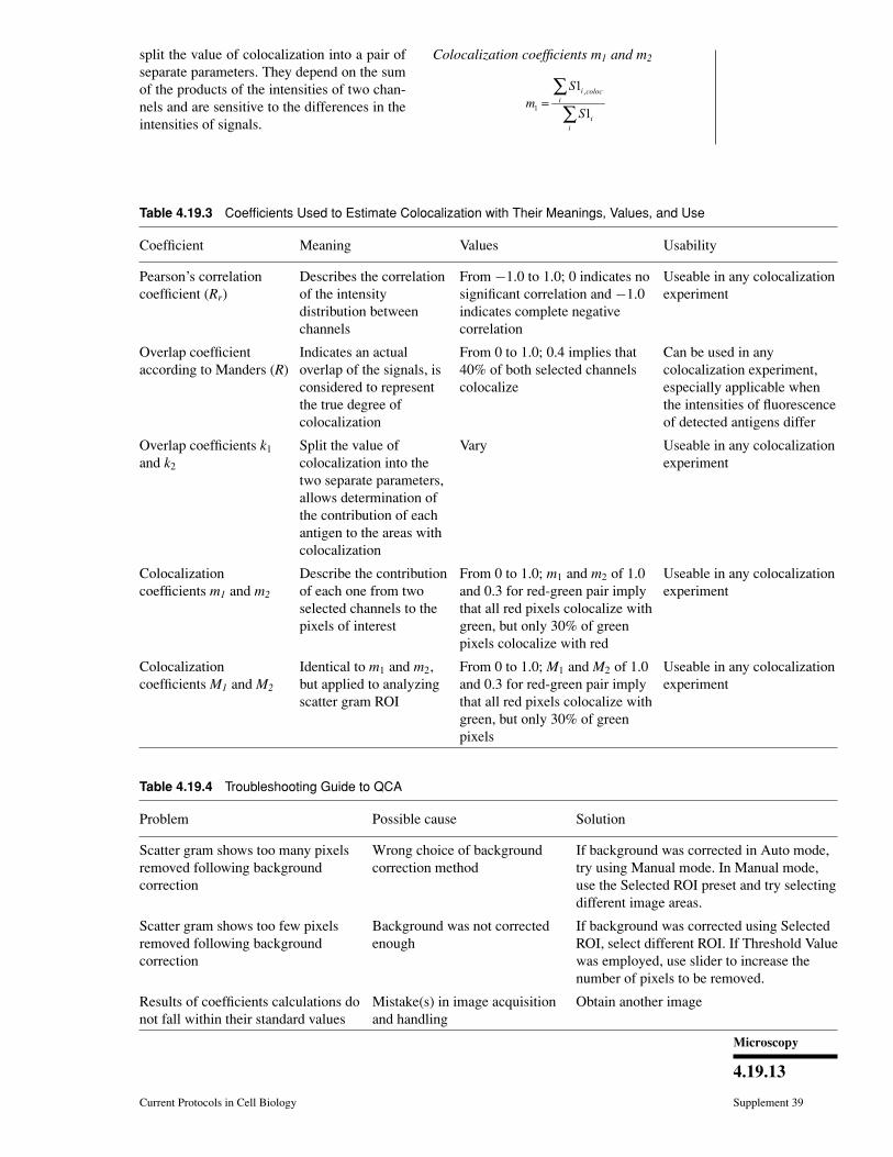
Table 4.19.3 Coefficients Used to Estimate Colocalization with Their Meanings, Values, and Use

Coefficient Meaning Values Usability

Pearson’s correlationcoefficient (Rr)

Describes the correlationof the intensitydistribution betweenchannels

From −1.0 to 1.0; 0 indicates nosignificant correlation and −1.0indicates complete negativecorrelation

Useable in any colocalizationexperiment

Overlap coefficientaccording to Manders (R)

Indicates an actualoverlap of the signals, isconsidered to representthe true degree ofcolocalization

From 0 to 1.0; 0.4 implies that40% of both selected channelscolocalize

Can be used in anycolocalization experiment,especially applicable whenthe intensities of fluorescenceof detected antigens differ

Overlap coefficients k1

and k2

Split the value ofcolocalization into thetwo separate parameters,allows determination ofthe contribution of eachantigen to the areas withcolocalization

Vary Useable in any colocalizationexperiment

Colocalizationcoefficients m1 and m2

Describe the contributionof each one from twoselected channels to thepixels of interest

From 0 to 1.0; m1 and m2 of 1.0and 0.3 for red-green pair implythat all red pixels colocalize withgreen, but only 30% of greenpixels colocalize with red


Colocalizationcoefficients M1 and M2

Identical to m1 and m2,but applied to analyzingscatter gram ROI

From 0 to 1.0; M1 and M2 of 1.0and 0.3 for red-green pair implythat all red pixels colocalize withgreen, but only 30% of greenpixels


Table 4.19.4 Troubleshooting Guide to QCA

Problem Possible cause Solution

Scatter gram shows too many pixelsremoved following backgroundcorrection

Wrong choice of backgroundcorrection method

If background was corrected in Auto mode,try using Manual mode. In Manual mode,use the Selected ROI preset and try selectingdifferent image areas.

Scatter gram shows too few pixelsremoved following backgroundcorrection

Background was not correctedenough

If background was corrected using SelectedROI, select different ROI. If Threshold Valuewas employed, use slider to increase thenumber of pixels to be removed.

Results of coefficients calculations donot fall within their standard values

Mistake(s) in image acquisitionand handling

Obtain another image


Analysis ofConfocal


Images

4.19.14


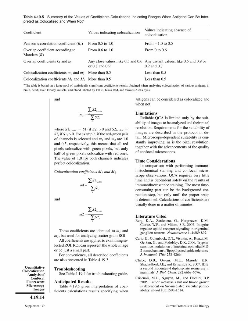
Table 4.19.5 Summary of the Values of Coefficients Calculations Indicating Ranges When Antigens Can Be Inter-preted as Colocalized and When Nota

Coefficient Values indicating colocalizationValues indicating absence ofcolocalization

Pearson’s correlation coefficient (Rr) From 0.5 to 1.0 From −1.0 to 0.5

Overlap coefficient according toManders (R)

From 0.6 to 1.0 From 0 to 0.6

Overlap coefficients k1 and k2 Any close values, like 0.5 and 0.6or 0.8 and 0.9

Any distant values, like 0.5 and 0.9 or0.2 and 0.7

Colocalization coefficients m1 and m2 More than 0.5 Less than 0.5

Colocalization coefficients M1 and M2 More than 0.5 Less than 0.5aThe table is based on a large pool of statistically significant coefficients results obtained when analyzing colocalization of various antigens inbrain, heart, liver, kidney, muscle, and blood labeled by FITC, Texas Red, and various Alexa dyes.

and

,

2

2

2

i coloci

ii

Sm

S=

∑∑

where S1i,coloc = S1i if S2i >0 and S2i,coloc =S2i if S1i >0. For example, if the red-green pairof channels is selected and m1 and m2 are 1.0and 0.5, respectively, this means that all redpixels colocalize with green pixels, but onlyhalf of green pixels colocalize with red ones.The value of 1.0 for both channels indicatesperfect colocalization.

Colocalization coefficients M1 and M2

,1

11

i coloci

ii

Sm

S=

∑∑

and

,2

22

i coloci

ii

Sm

S=

∑∑

These coefficients are identical to m1 andm2, but used for analyzing scatter gram ROI.

All coefficients are applied to examining se-lected ROI. ROI can represent the whole imageor be just a small part.

For convenience, all described coefficientsare also presented in Table 4.19.3.

TroubleshootingSee Table 4.19.4 for troubleshooting guide.

Anticipated ResultsTable 4.19.5 gives interpretation of coef-

ficients calculations results specifying when

antigens can be considered as colocalized andwhen not.

LimitationsReliable QCA is limited only by the suit-

ability of images to be analyzed and their pixelresolution. Requirements for the suitability ofimages are described in the protocol in de-tail. Microscope-dependent suitability is con-stantly improving, as is the pixel resolution,together with the advancements of the qualityof confocal microscopes.

Time ConsiderationsIn comparison with performing immuno-

histochemical staining and confocal micro-scope observations, QCA requires very littletime and is dependent solely on the results ofimmunofluorescence staining. The most time-consuming part can be the background cor-rection step, but only until the proper setupis determined. Calculations of coefficients areusually done in a matter of minutes.

Literature CitedBerg, K.A., Zardeneta, G., Hargreaves, K.M.,

Clarke, W.P., and Milam, S.B. 2007. Integrinsregulate opioid receptor signaling in trigeminalganglion neurons. Neuroscience 144:889-897.

Cario, E., Golenbock, D.T., Visintin, A., Runzi, M.,Gerken, G., and Podolsky, D.K. 2006. Trypsin-sensitive modulation of intestinal epithelial MD-2 as mechanism of lipopolysaccharide tolerance.J. Immunol. 176:4258-4266.

Clizbe, D.B., Owens, M.L., Masuda, K.R.,Shackelford, J.E., and Krisans, S.K. 2007. IDI2,a second isopentenyl diphosphate isomerase inmammals. J. Biol. Chem. 282:6668-6676.

Criscuoli, M.L., Nguyen, M., and Eliceiri, B.P.2005. Tumor metastasis but not tumor growthis dependent on Src-mediated vascular perme-ability. Blood 105:1508-1514.

Microscopy

4.19.15


Desplanques, A.S., Nauwynck, H.J., Tilleman, K.,Deforce, D., and Favoreel, H.W. 2007. Tyro-sine phosphorylation and lipid raft associationof pseudorabies virus glycoprotein E duringantibody-mediated capping. Virology 362:60-66.

Dombrowski, F., Stieger, B., and Beuers, U.2006. Tauroursodeoxycholic acid inserts the bilesalt export pump into canalicular membranesof cholestatic rat liver. Lab. Invest. 86:166-174.

Gerloff, T., Stieger, B., Hagenbuch, B., Madon, J.,Landmann, L., Roth, J., Hofmann, A.F., andMeier, P.J. 1998. The sister of P-glycoproteinrepresents the canalicular bile salt export pumpof mammalian liver. J. Biol. Chem. 273:10046-10050.

Head, B.P., Patel, H.H, Roth, D.M., Murray, F.,Swaney, J.S., Niesman, I.R., Farquhar, M.G.,and Insel, P.A. 2006. Microtubules and actinmicrofilaments regulate lipid raft/caveolae lo-calization of adenylyl cyclase signaling compo-nents. J. Biol. Chem. 281:26391-26399.

Kato, T., Muraski, J., Chen, Y., Tsujita, Y., Wall,J., Glembotski, C.C., Schaefer, E., Beckerle,M., and Sussman, M.A. 2005. Atrial natri-uretic peptide promotes cardiomyocyte survivalby cGMP-dependent nuclear accumulation ofzyxin and Akt. J. Clin. Invest. 115:2716-2730.

Konig, J., Nies, A.T., Cui, Y., Leier, I., andKeppler, D. 1999. Conjugate export pumps ofthe multidrug resistance protein (MRP) family:Localization, substrate specificity, and MRP2-mediated drug resistance. Biochim. Biophys.Acta 1461:377-394.

Landmann, L. and Marbet, P. 2004. Colocaliza-tion analysis yields superior results after imagerestoration. Microsc. Res. Tech. 64:103-112.

Lippincott-Schwartz, J., Snapp, E., and Kenworthy,A. 2001. Studying protein dynamics in livingcells. Nat. Rev. Mol. Cell Biol. 2:444-456.

Manders, E.M.M., Verbeek, F.J., and Aten,J.A. 1993. Measurement of co-localization ofobjects in dual-colour confocal images.J. Microsc. 169:375-382.

Mutch, C.M., Sanyal, R., Unruh, T.L.,Grigoriou, L., Zhu, M., Zhang, W., andDeans, J.P. 2007. Activation-induced endo-cytosis of the raft-associated transmembraneadaptor protein LAB/NTAL in B lymphocytes:Evidence for a role in internalization of the Bcell receptor. Int. Immunol. 19:19-30.

North, A.J. 2006. Seeing is believing? A beginners’guide to practical pitfalls in image acquisition.J. Cell Biol. 172:9-18.

Patel, H.H., Head, B.P., Petersen, H.N., Niesman,I.R., Huang, D., Gross, G.J., Insel, P.A., andRoth, D.M. 2006. Protection of adult rat car-diac myocytes from ischemic cell death: Roleof caveolar microdomains and delta-opioid re-ceptors. Am. J. Physiol. Heart Circ. Physiol.291:H344-H350.

Rey, O., Young, S.H., Papazyan, R., Shapiro, M.S.,and Rozengurt, E. 2006. Requirement of the

TRPC1 cation channel in the generation of tran-sient Ca2+ oscillations by the calcium-sensingreceptor. J. Biol. Chem. 281:38730-38737.

Rocker, C., Manolov, D.E., Kuzmenkina, E.V.,Tron, K., Slatosch, H., Torzewski, J., andNienhaus, G.U. 2007. Affinity of C-reactive pro-tein toward FcgammaRI is strongly enhancedby the gamma-chain. Am. J. Pathol. 170:755-763.

Smallcombe, A. 2001. Multicolor imaging: Theimportant question of co-localization. Biotech-niques 30:1240-1246.

Swaney, J.S., Patel, H.H., Yokoyama, U., Head,B.P., Roth, D.M., and Insel, P.A. 2006. Focaladhesions in (myo)fibroblasts scaffold adenylylcyclase with phosphorylated caveolin. J. Biol.Chem. 281:17173-17179.

Tsutsumi, Y.M., Patel, H.H., Huang, D., and Roth,D.M. 2006. Role of 12-lipoxygenase in volatileanesthetic-induced delayed preconditioning inmice. Am. J. Physiol. Heart Circ. Physiol.291:H979-H983.

Van Acker, G.J., Weiss, E., Steer, M.L., andPerides, G. 2007. Cause-effect relationshipsbetween zymogen activation and other earlyevents in secretagogue-induced acute pancreati-tis. Am. J. Physiol. Gastrointest. Liver Physiol.292:G1738-G1746.

Watanabe, T., Sorensen, E.M., Naito, A., Schott,M., Kim, S., and Ahlquist, P. 2007. Involvementof host cellular multivesicular body functions inhepatitis B virus budding. Proc. Natl. Acad. Sci.U. S. A. 104:10205-10210.

Zinchuk, V.S., Okada, T., Akimaru, K., andSeguchi, H. 2002. Asynchronous expression andcolocalization of Bsep and Mrp2 during devel-opment of rat liver. Am. J. Physiol. Gastrointest.Liver Physiol. 282:G540-G548.

Zinchuk, O., Fukushima, A., Hangstefer, E., andUeno, H. 2004. Dynamics of PAF-induced con-junctivitis reveals differential expression of PAFreceptor by macrophages and eosinophils in therat. Cell Tissue Res. 317:265-277.

Zinchuk, O., Fukushima, A., Zinchuk, V., Fukata,K., and Ueno, H. 2005a. Direct action of plateletactivating factor (PAF) induces eosinophil ac-cumulation and enhances expression of PAFreceptors in conjunctivitis. Mol. Vis. 11:114-123.

Zinchuk, V., Zinchuk, O., and Okada, T. 2005b. Ex-perimental LPS-induced cholestasis alters sub-cellular distribution and affects colocalizationof Mrp2 and Bsep proteins: A quantitative colo-calization study. Microsc. Res. Tech. 67:65-70.

Key ReferencesManders et al., 1993. See above.First description of the correlation coefficient andexamples of its use.

Smallcombe, 2003. See above.Practical look at colocalization, some critical viewsand advice for performing colocalization experi-ments.


Analysis ofConfocal


Images

4.19.16


North, 2006. See above.Review with focus on proper interpretation of theresults of fluorescence microscopy studies, draw-backs and limitations of biological imagery.

Internet Resourceshttp://homepage.mac.com/colocalizerpro/Web site of CoLocalization Research Software, cre-ators of CoLocalizer Pro and CoLocalizer Expresssoftware applications used for quantitative estima-tion of colocalization.

Documents

Quantitative Colocalization Analysis of Confocal Fluorescence