Acquiring and Analyzing Data for Colocalization ... · Acquiring and Analyzing Data for Colocalization Experiments in AIM ... The Basics To initiate a colocalization analysis in ZEN,

Acquiring and Analyzing Data for

Colocalization Experiments in AIM or ZEN Software

Colocalization analysis is one of the most widespread applications used in fluorescence microscopy. As any two channel image can be analyzed for colocalization, it is a seemingly easy application to perform. However, there are many factors which can lead to false colocalization; careful consideration must be taken in order to ensure that artifacts are avoided. Any questions or concerns can be directed to the ZEISS Product and Applications Support group at 1-800-509-3905 or [email protected]

mailto:[email protected]

2 Carl Zeiss MicroImaging Maya Everett

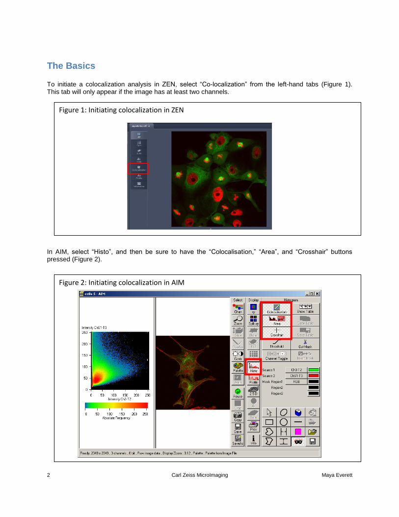
The Basics To initiate a colocalization analysis in ZEN, select “Co-localization” from the left-hand tabs (Figure 1). This tab will only appear if the image has at least two channels.

In AIM, select “Histo”, and then be sure to have the “Colocalisation,” “Area”, and “Crosshair” buttons pressed (Figure 2).

Figure 1: Initiating colocalization in ZEN

Figure 2: Initiating colocalization in AIM


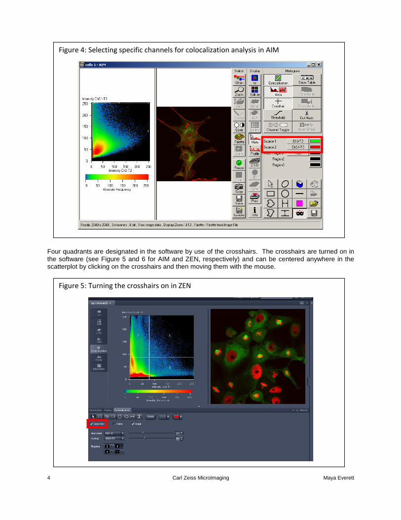
Colocalization analysis is performed on a pixel by pixel basis. Every pixel in the image is plotted in the scatter diagram based on its intensity level from each channel. The color in the scatterplot represents the number of pixels that are plotted in that region. In this example, green intensity is shown on the x-axis and red intensity is shown on the y-axis. You can select which channel you want on which axis (See Figure 3 for ZEN and Figure 4 for AIM). For an image with three channels or more, only two channels can be selected for colocalization analysis.

Figure 3: Selecting specific channels for colocalization analysis in ZEN


Four quadrants are designated in the software by use of the crosshairs. The crosshairs are turned on in the software (see Figure 5 and 6 for AIM and ZEN, respectively) and can be centered anywhere in the scatterplot by clicking on the crosshairs and then moving them with the mouse.

Figure 4: Selecting specific channels for colocalization analysis in AIM

Figure 5: Turning the crosshairs on in ZEN


The lower left, unlabeled quadrant in the scatterplot represents pixels that have low intensity levels in both channels (Quadrant 4); these pixels are referred to as background and are not taken into consideration for colocalization analysis. In this example, Quadrants 1 represent pixels that have high green intensities and low red intensities and Quadrant 2 represents pixels that have high red intensities and low green intensities. Quadrant 3 represents pixels with high intensity levels in both green and red. These pixels are considered to be colocalized. One method of examining colocalized pixels between green and red channels is to look for the appearance of yellow when these two colors blend together. An easier way of viewing colocalized pixels is to false colors pixels from Quadrant 3 in white (or other color). Quadrants 1 and 2 can also be false colored, if necessary. See Figures 7 and 8 for visualization on how to false color the different quadrants of the scatterplot in ZEN and AIM, respectively.

Figure 6: To view the crosshairs, be sure that the Crosshair button is pressed.


Figure 7: Select Quadrant 3 and set to white for easier visualization of the pixels exhibiting colocalization. The other three quadrants can also be false colored in the same fashion.

Figure 8: Select Quadrant 3 and set to white for easier visualization of the pixels exhibiting colocalization. The other two quadrants, except for Quadrant 4, can also be false colored in the same fashion.


Experimental Set-Up As pixel intensity dictates its position on the scatterplot, it is critical that all imaging parameters which influence the intensity of the image remain the same for all data acquisition. This includes: objective lens, lamp power or laser power, filter sets or wavelength collections, acquisition speed, camera or PMT settings, etc. The type of mounting media should also be kept constant as different types may exhibit varying levels of autofluorescence or affect the intensity levels of the fluorophores. Similarly, imaging through different types of material, such as a glass coverslip versus a plastic bottom dish, will affect the intensity of the resulting image.

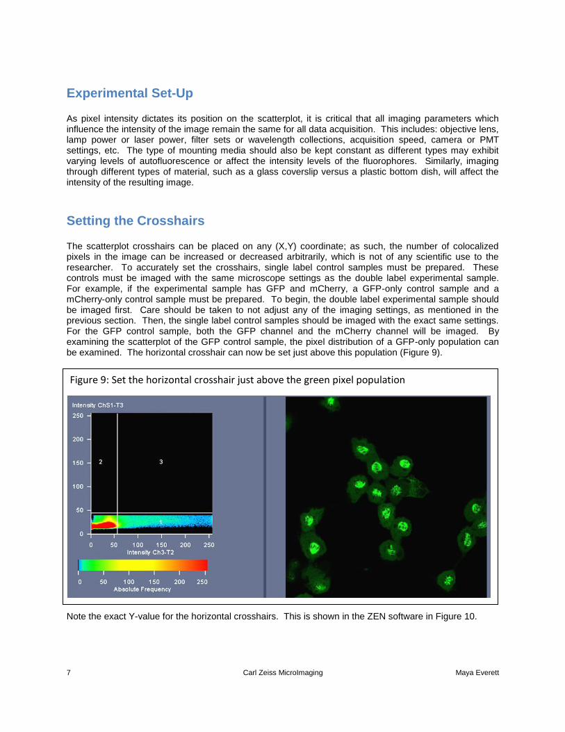
Setting the Crosshairs The scatterplot crosshairs can be placed on any (X,Y) coordinate; as such, the number of colocalized pixels in the image can be increased or decreased arbitrarily, which is not of any scientific use to the researcher. To accurately set the crosshairs, single label control samples must be prepared. These controls must be imaged with the same microscope settings as the double label experimental sample. For example, if the experimental sample has GFP and mCherry, a GFP-only control sample and a mCherry-only control sample must be prepared. To begin, the double label experimental sample should be imaged first. Care should be taken to not adjust any of the imaging settings, as mentioned in the previous section. Then, the single label control samples should be imaged with the exact same settings. For the GFP control sample, both the GFP channel and the mCherry channel will be imaged. By examining the scatterplot of the GFP control sample, the pixel distribution of a GFP-only population can be examined. The horizontal crosshair can now be set just above this population (Figure 9).

Note the exact Y-value for the horizontal crosshairs. This is shown in the ZEN software in Figure 10.

Figure 9: Set the horizontal crosshair just above the green pixel population


To view the crosshair settings in AIM, you will need to click on the Threshold button (Figure 11).

Figure 10: The exact crosshair settings are shown in the Colocalization tab.


This process is repeated with the mCherry control sample to set the vertical crosshair. See Figure 12.

Figure 11: The exact crosshair settings are shown by opening the Threshold submenu.


After setting the crosshairs for the mCherry-only sample, check the exact threshold value for the vertical crosshair as shown in Figures 10 and 11. Once the exact (X,Y) coordinates are determined by using the control samples, they must be kept the same for analysis of the double-label experimental samples. This ensures that any pixels localized to Quadrant 3 are due to significant intensity levels of both labels in those pixels and not from changes in the sample preparation, acquisition settings, or random assignment of the crosshair coordinates.

Analyzing the Data The software will automatically analyze many different measurements from the scatterplot. The table must be displayed in order to view these numbers. How to select the table function is shown in Figures 13 and 14 for ZEN and AIM, respectively. It is essential to understand what the numbers mean in order to interpret them correctly.

Figure 12: Setting the crosshairs for the red channel using a mCherry-only control sample


Figure 13: Check the Table box for the calculations to appear below the scatterplot and the image. Use the horizontal scrollbar to view the table values to the right.

Figure 13: Press the Show Table button for the calculations to appear below the scatterplot and image. Use the horizontal scrollbar to view the table values to the right.


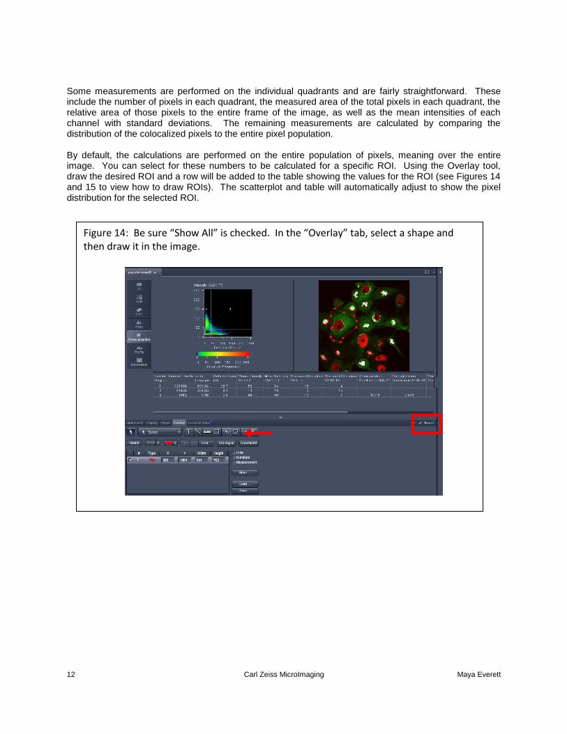
Some measurements are performed on the individual quadrants and are fairly straightforward. These include the number of pixels in each quadrant, the measured area of the total pixels in each quadrant, the relative area of those pixels to the entire frame of the image, as well as the mean intensities of each channel with standard deviations. The remaining measurements are calculated by comparing the distribution of the colocalized pixels to the entire pixel population. By default, the calculations are performed on the entire population of pixels, meaning over the entire image. You can select for these numbers to be calculated for a specific ROI. Using the Overlay tool, draw the desired ROI and a row will be added to the table showing the values for the ROI (see Figures 14 and 15 to view how to draw ROIs). The scatterplot and table will automatically adjust to show the pixel distribution for the selected ROI.

Figure 14: Be sure “Show All” is checked. In the “Overlay” tab, select a shape and then draw it in the image.


Colocalization Coefficients The most useful of the colocalization measurements for standard biology applications are the colocalization coefficients. These were derived in the following paper: Manders et al., (1993) Measurement of co-localization of objects in dual-colour confocal images. Journal of Microscopy 169:375-82. The colocalization coefficients are measured for each channel. They are calculated by summing the pixels in the colocalized region (Quadrant 3) and then dividing by the sum of pixels either in Channel 1 (Quadrant 1 + Quadrant 3) or in Channel 2 (Quadrant 2 + Quadrant 3). Each pixel has a value of 1. The colocalization coefficient values will range from 0 to 1. The equation for the green and red colocalization coefficients are shown here:

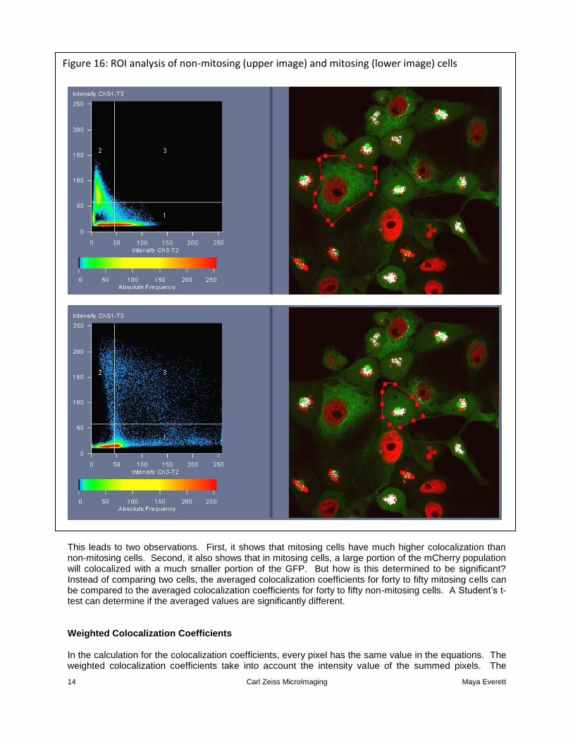
In the example for a non-mitosing cell (Figure 16, upper image), the software calculates the colocalization coefficient for Channel 1, GFP, as 0.0% and for Channel 2, mCherry, as 0.1%. However, when the ROI is drawn around a cell in mitosis (Figure 16, lower image) the GFP colocalization coefficient is measured to be 10.3% and the mCherry colocalization is measured to be 70.0%.

Figure 15: Select ROIs from the Histo submenu for colocalization analysis


This leads to two observations. First, it shows that mitosing cells have much higher colocalization than non-mitosing cells. Second, it also shows that in mitosing cells, a large portion of the mCherry population will colocalized with a much smaller portion of the GFP. But how is this determined to be significant? Instead of comparing two cells, the averaged colocalization coefficients for forty to fifty mitosing cells can be compared to the averaged colocalization coefficients for forty to fifty non-mitosing cells. A Student’s t-test can determine if the averaged values are significantly different. Weighted Colocalization Coefficients In the calculation for the colocalization coefficients, every pixel has the same value in the equations. The weighted colocalization coefficients take into account the intensity value of the summed pixels. The

Figure 16: ROI analysis of non-mitosing (upper image) and mitosing (lower image) cells


weighted colocalization coefficients use the same equation as the colocalization coefficients, but the value for each pixel is equal to its intensity value. Their values will range from 0 to 1. In this analysis, a pixel with bright intensity represents a higher number of fluorophores than a pixel with low intensity. Whereas the unweighted colocalization coefficients calculate values based on the pixel population, the weighted colocalization coefficients calculate values based on the estimated fluorophore population. In our previous example with the mitosing cells, the colocalized coefficient for GFP is 10.3% and for mCherry is 70.0%. The weighted colocalization coefficients are 15.9% and 67.0%, respectively. Because the weighted colocalization coefficient for GFP is higher than the non-weighted colocalization coefficient, it means that there are brighter pixels in the colocalized region than in the non-colocalized region. Similarly, the weighted colocalization for mCherry is lower than the non-weighted colocalization, which means that there are brighter pixels in the non-colocalized regions. A common question is whether to use weighted or non-weighted colocalization coefficients when analyzing data. This is for the researcher to determine. It is worth comparing both values during analysis. It is important to report which method you use and interpret it accordingly. Pearson’s Correlation Coefficient and Derivatives The equation for the colocalization coefficients were derived from the Pearson’s Correlation Coefficient, which provides information about the similarity of shape between two patterns:

Because each pixel is subtracted by the average pixel intensity, the value for Correlation R can range from -1 to 1. A value of 1 would mean that the patterns are perfectly similar, every pixel that contains GFP also contains mCherry, while a value of -1 would mean that the patterns are perfectly opposite, every pixel that contains GFP does not contain mCherry and vice versa. If the two channels are correlated, meaning if the values are close to 1 or -1, it means that the pattern in one channel can be predicted by the pattern of the other channel. Squaring the Correlation R will generate Correlation RxR, also called the coefficient of determination. This term predicts the degree of change you would expect in one channel based in changes in the other channel. Manders and colleagues thought that negative values that are often found in Correlation R are difficult to interpret when it is the degree of overlap that is of interest to researchers. They removed this average subtraction to generate a new equation, called the Overlap Coefficient.

The values for the overlap coefficient range from 0 to 1. The numerator in the Overlap Coefficient equation is only positive for pixels that contain significant intensity levels from both channels and is proportional to colocalized pixels; whereas the denominator is proportional to all pixels with significant intensity values, regardless of colocalization. An Overlap Coefficient with a value of 1 represents perfectly colocalized pixels. However, this measurement can be affected by the ratio of pixels between the channels. Using our previous example of the mitosing cell, even though there is strong colocalization between the GFP and mCherry, there are more green pixels than red pixels in the ROI of the mitosing


cells. Even though there is a strong colocalization between the green and red pixels, the mismatch in ratio between the pixels will lower the Overlap Coefficient. Because of this dependence on the ratio between the two channels, Manders and colleagues derived the Colocalization Coefficients, described above, which are the most useful for biological applications. More Information The ZEISS Campus website is a wonderful resource for information on microscopy. Review articles on colocalization can be found in the Reference Library section of the ZEISS Campus website, www.zeiss.com/campus. To jump straight to the specific section on colocalization, please use the following link: http://zeiss-campus.magnet.fsu.edu/referencelibrary/colocalization.html

Documents

Acquiring and Analyzing Data for Colocalization ... · Acquiring and Analyzing Data for Colocalization Experiments in AIM ... The Basics To initiate a colocalization analysis in ZEN,