�

�

�

�

Collaborative MIMO Networks

Dr Mischa Dohler

Senior Research Expert

France Telecom R&D, TECH/IDEA

mischa.dohler@orange-ftgroup.com

Journee GDR, ENST, Paris, March 2007 1

�

�

�

�

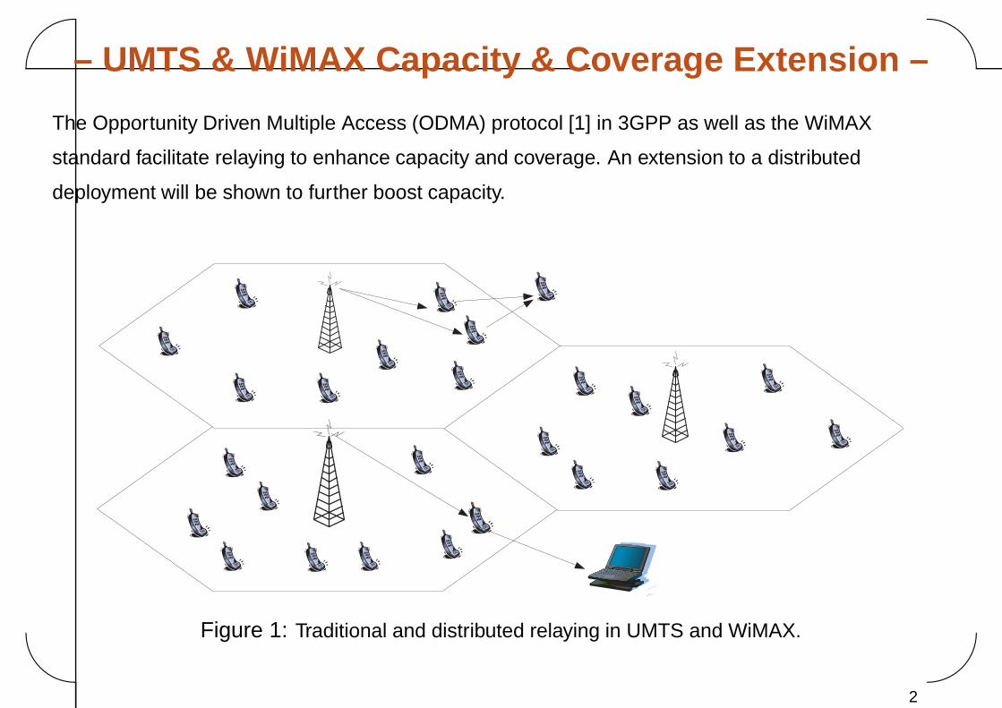
– UMTS & WiMAX Capacity & Coverage Extension –

The Opportunity Driven Multiple Access (ODMA) protocol [1] in 3GPP as well as the WiMAX

standard facilitate relaying to enhance capacity and coverage. An extension to a distributed

deployment will be shown to further boost capacity.

Figure 1: Traditional and distributed relaying in UMTS and WiMAX.

2

�

�

�

�

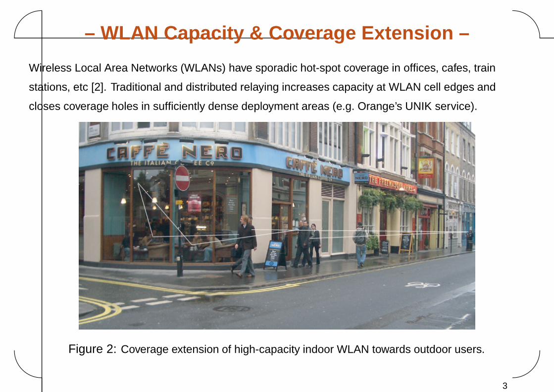
– WLAN Capacity & Coverage Extension –

Wireless Local Area Networks (WLANs) have sporadic hot-spot coverage in offices, cafes, train

stations, etc [2]. Traditional and distributed relaying increases capacity at WLAN cell edges and

closes coverage holes in sufficiently dense deployment areas (e.g. Orange’s UNIK service).

Figure 2: Coverage extension of high-capacity indoor WLAN towards outdoor users.

3

�

�

�

�

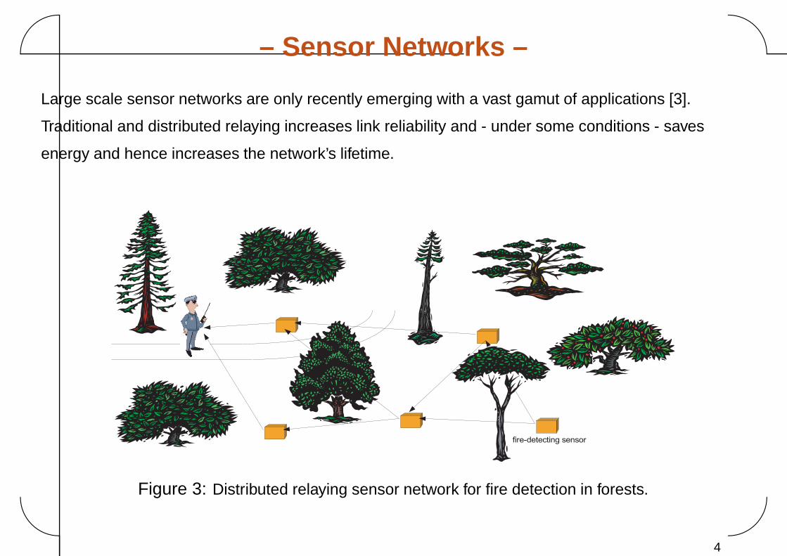
– Sensor Networks –

Large scale sensor networks are only recently emerging with a vast gamut of applications [3].

Traditional and distributed relaying increases link reliability and - under some conditions - saves

energy and hence increases the network’s lifetime.

fire-detecting sensor

Figure 3: Distributed relaying sensor network for fire detection in forests.

4

�

�

�

�

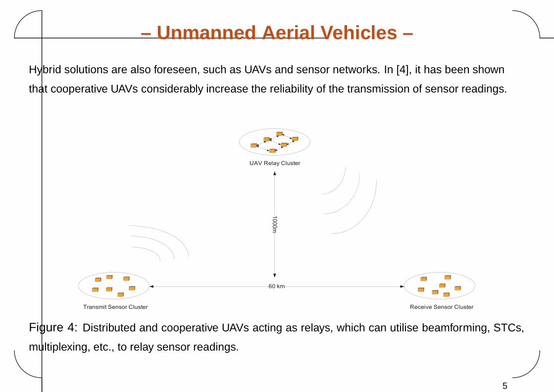
– Unmanned Aerial Vehicles –

Hybrid solutions are also foreseen, such as UAVs and sensor networks. In [4], it has been shown

that cooperative UAVs considerably increase the reliability of the transmission of sensor readings.

Transmit Sensor Cluster Receive Sensor Cluster

60 km

UAV Relay Cluster

10

00

m

Figure 4: Distributed and cooperative UAVs acting as relays, which can utilise beamforming, STCs,

multiplexing, etc., to relay sensor readings.

5

�

�

�

�

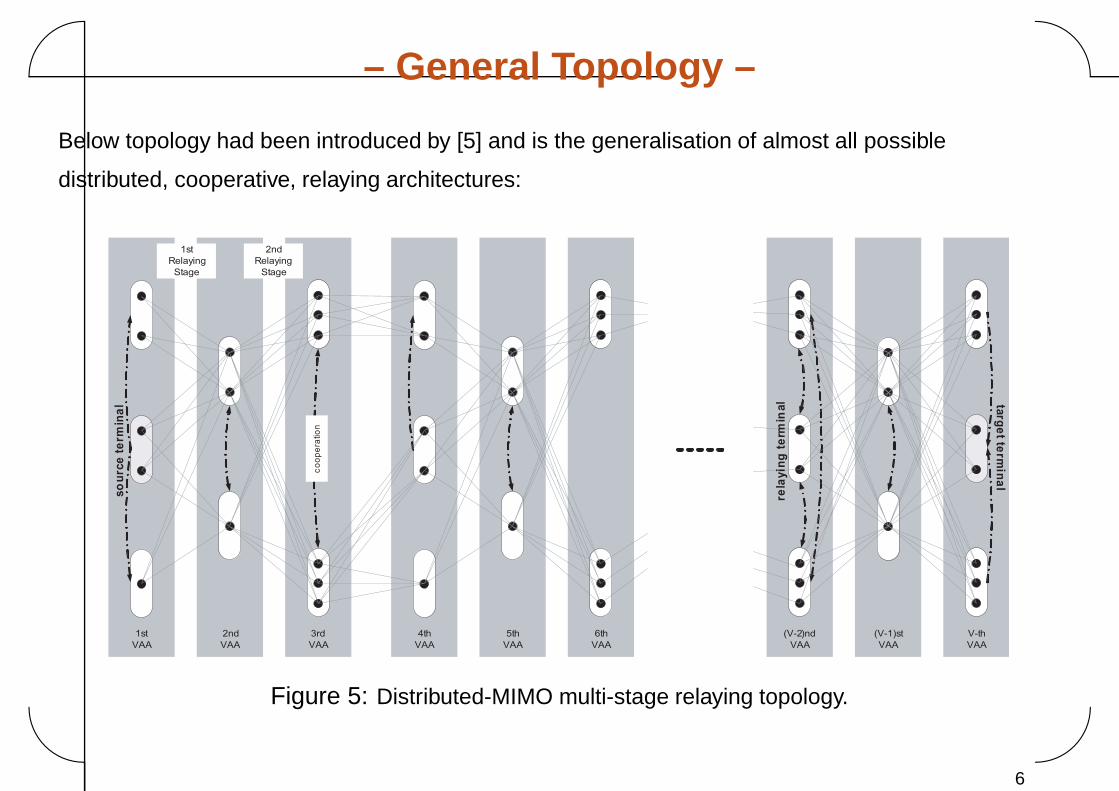
– General Topology –

Below topology had been introduced by [5] and is the generalisation of almost all possible

distributed, cooperative, relaying architectures:

6th

VAA

5th

VAA

4th

VAA

(V-2)nd

VAA

(V-1)st

VAA

V-th

VAA

targ

et te

rmin

al

3rd

VAA

2nd

VAA

1st

VAA

so

urc

e t

erm

ina

l

1st

Relaying

Stage

2nd

Relaying

Stage

co

op

era

tion

rela

yin

g t

erm

inal

Figure 5: Distributed-MIMO multi-stage relaying topology.

6

�

�

�

�

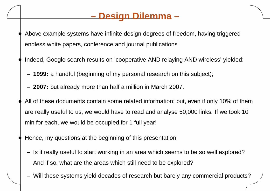
– Design Dilemma –

• Above example systems have infinite design degrees of freedom, having triggered

endless white papers, conference and journal publications.

• Indeed, Google search results on ’cooperative AND relaying AND wireless’ yielded:

– 1999: a handful (beginning of my personal research on this subject);

– 2007: but already more than half a million in March 2007.

• All of these documents contain some related information; but, even if only 10% of them

are really useful to us, we would have to read and analyse 50,000 links. If we took 10

min for each, we would be occupied for 1 full year!

• Hence, my questions at the beginning of this presentation:

– Is it really useful to start working in an area which seems to be so well explored?

And if so, what are the areas which still need to be explored?

– Will these systems yield decades of research but barely any commercial products?

7

�

�

�

�

– Outline –

1. Preliminaries

2. Hardware Issues

3. Channel Characterisation

4. MAC and Cross-Layer Design

5. Conclusions & Road Ahead

8

�

�

�

�

PART 1PRELIMINARIES

9

�

�

�

�

Useful Definitions

10

�

�

�

�

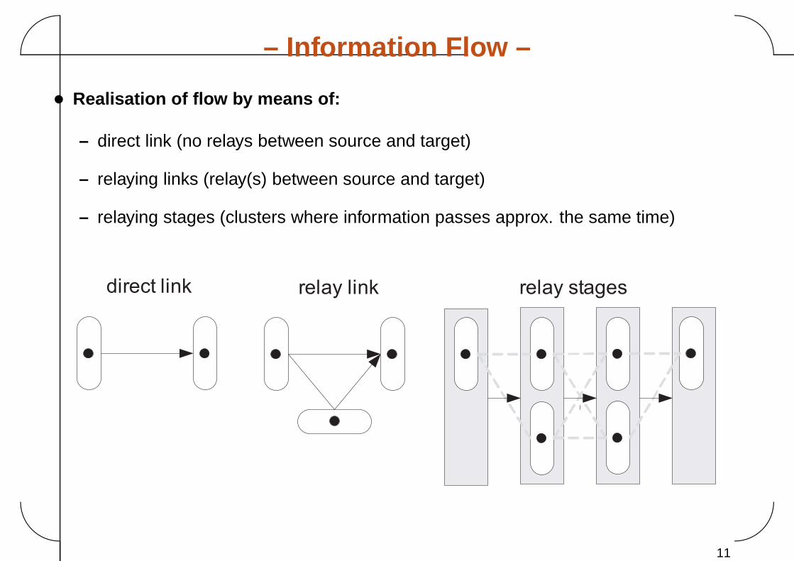
– Information Flow –

• Realisation of flow by means of:

– direct link (no relays between source and target)

– relaying links (relay(s) between source and target)

– relaying stages (clusters where information passes approx. the same time)

direct link relay link relay stages

11

�

�

�

�

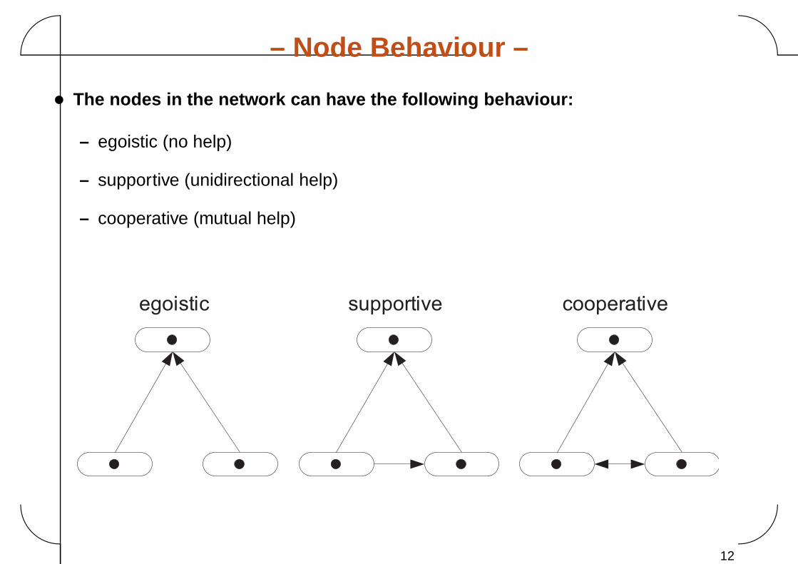
– Node Behaviour –

• The nodes in the network can have the following behaviour:

– egoistic (no help)

– supportive (unidirectional help)

– cooperative (mutual help)

egoistic supportive cooperative

12

�

�

�

�

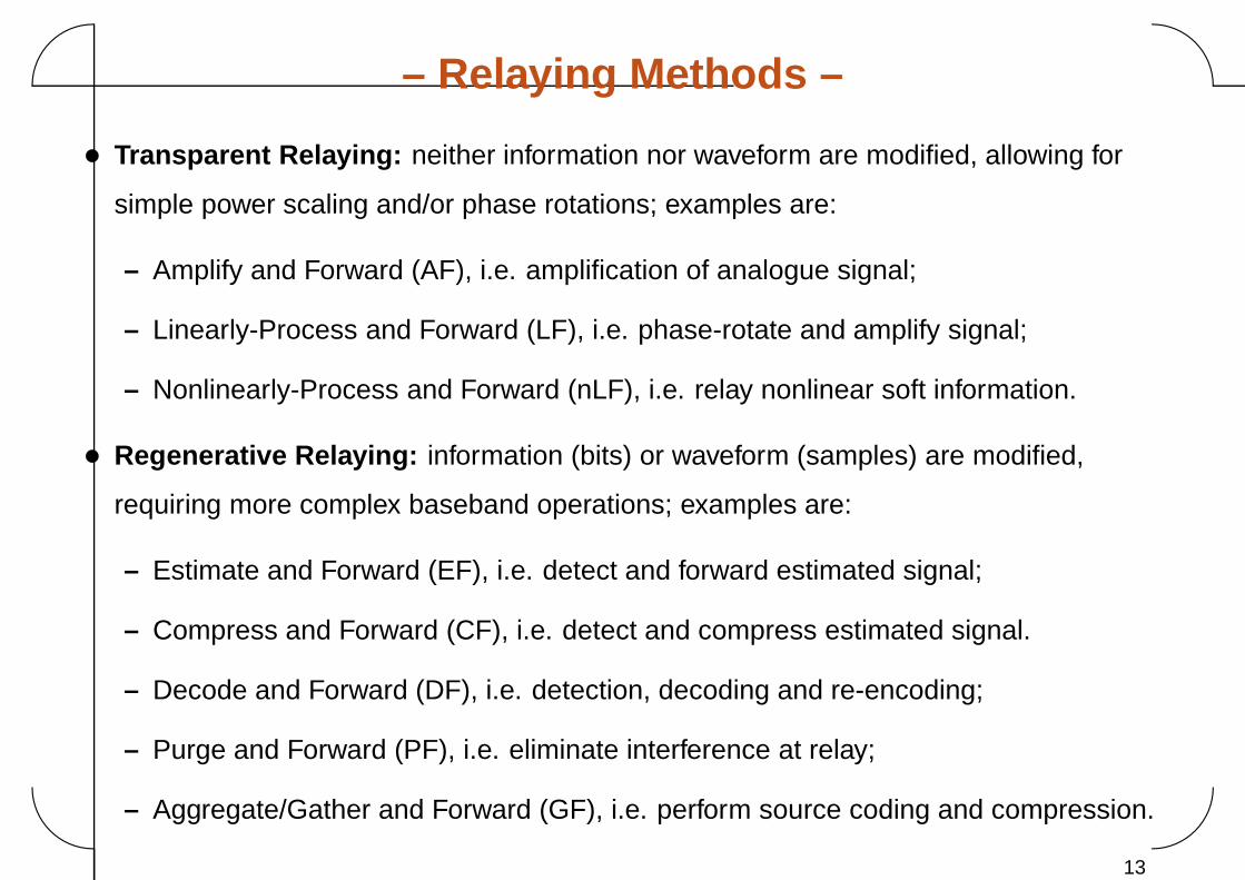
– Relaying Methods –

• Transparent Relaying: neither information nor waveform are modified, allowing for

simple power scaling and/or phase rotations; examples are:

– Amplify and Forward (AF), i.e. amplification of analogue signal;

– Linearly-Process and Forward (LF), i.e. phase-rotate and amplify signal;

– Nonlinearly-Process and Forward (nLF), i.e. relay nonlinear soft information.

• Regenerative Relaying: information (bits) or waveform (samples) are modified,

requiring more complex baseband operations; examples are:

– Estimate and Forward (EF), i.e. detect and forward estimated signal;

– Compress and Forward (CF), i.e. detect and compress estimated signal.

– Decode and Forward (DF), i.e. detection, decoding and re-encoding;

– Purge and Forward (PF), i.e. eliminate interference at relay;

– Aggregate/Gather and Forward (GF), i.e. perform source coding and compression.

13

�

�

�

�

Key Milestones

14

�

�

�

�

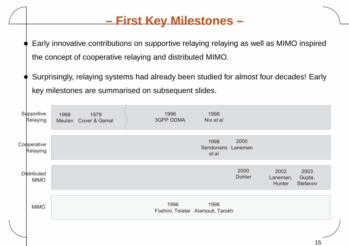
– First Key Milestones –

• Early innovative contributions on supportive relaying relaying as well as MIMO inspired

the concept of cooperative relaying and distributed MIMO.

• Surprisingly, relaying systems had already been studied for almost four decades! Early

key milestones are summarised on subsequent slides.

Supportive

Relaying

Cooperative

Relaying

1968

Meulen

1979

Cover & Gamal

2000

Dohler2002

Laneman,

Hunter

2003

Gupta,

Stefanov

2000

Laneman

1998

Sendonaris

et al

Distributed

MIMO

1996

3GPP ODMA

1998

Nix et al

MIMO1996

Foshini, Telatar

1998

Alamouti, Tarokh

15

�

�

�

�

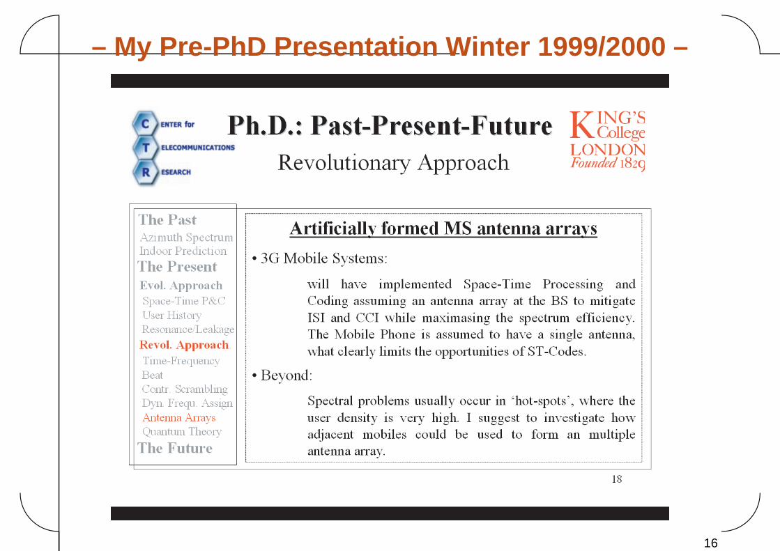
– My Pre-PhD Presentation Winter 1999/2000 –

16

�

�

�

�

Design Challenges

17

�

�

�

�

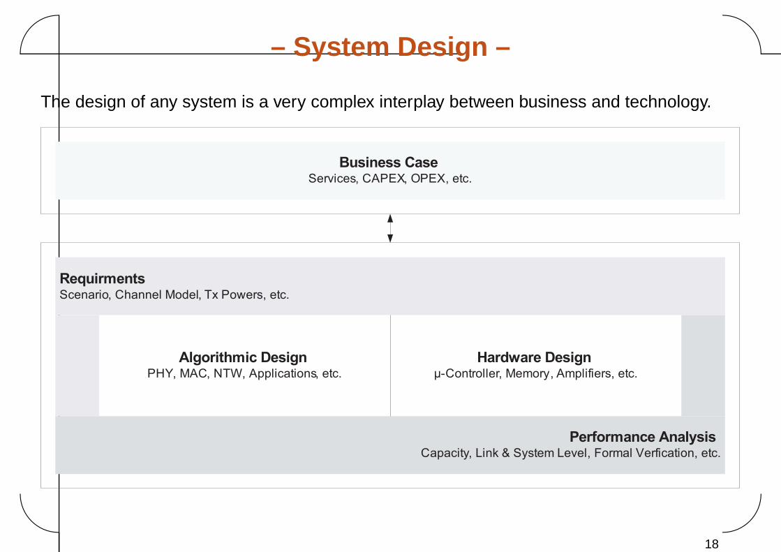
– System Design –

The design of any system is a very complex interplay between business and technology.

Business CaseServices, CAPEX, OPEX, etc.

RequirmentsScenario, Channel Model, Tx Powers, etc.

Performance AnalysisCapacity, Link & System Level, Formal Verfication, etc.

Algorithmic DesignPHY, MAC, NTW, Applications, etc.

Hardware Designµ-Controller, Memory, Amplifiers, etc.

18

�

�

�

�

PART 2HARDWARE ISSUES

19

�

�

�

�

Transparent Transceiver Design

20

�

�

�

�

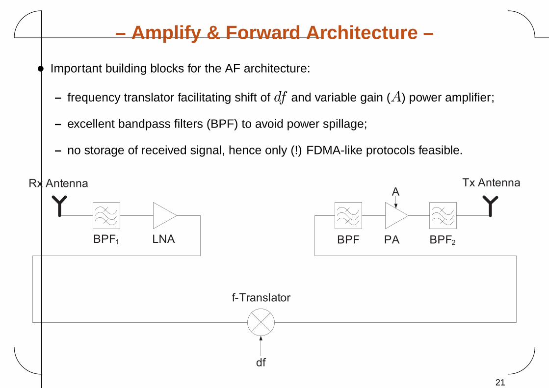
– Amplify & Forward Architecture –

• Important building blocks for the AF architecture:

– frequency translator facilitating shift of df and variable gain (A) power amplifier;

– excellent bandpass filters (BPF) to avoid power spillage;

– no storage of received signal, hence only (!) FDMA-like protocols feasible.

f-Translator

df

Rx Antenna

BPF1 LNA BPF PA

A

BPF2

Tx Antenna

21

�

�

�

�

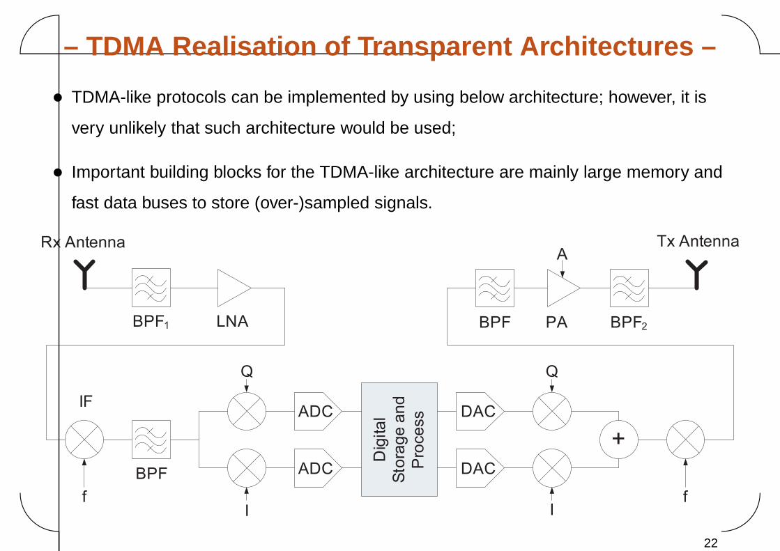
– TDMA Realisation of Transparent Architectures –

• TDMA-like protocols can be implemented by using below architecture; however, it is

very unlikely that such architecture would be used;

• Important building blocks for the TDMA-like architecture are mainly large memory and

fast data buses to store (over-)sampled signals.

Rx Antenna

BPF1 LNA

IF

f

BPF PA

A

BPF2

Tx Antenna

BPF

I

Q

ADC

ADC

Dig

ita

l

Sto

rag

e a

nd

Pro

ce

ss DAC

DAC

I

Q

+

f

22

�

�

�

�

Regenerative Transceiver Design

23

�

�

�

�

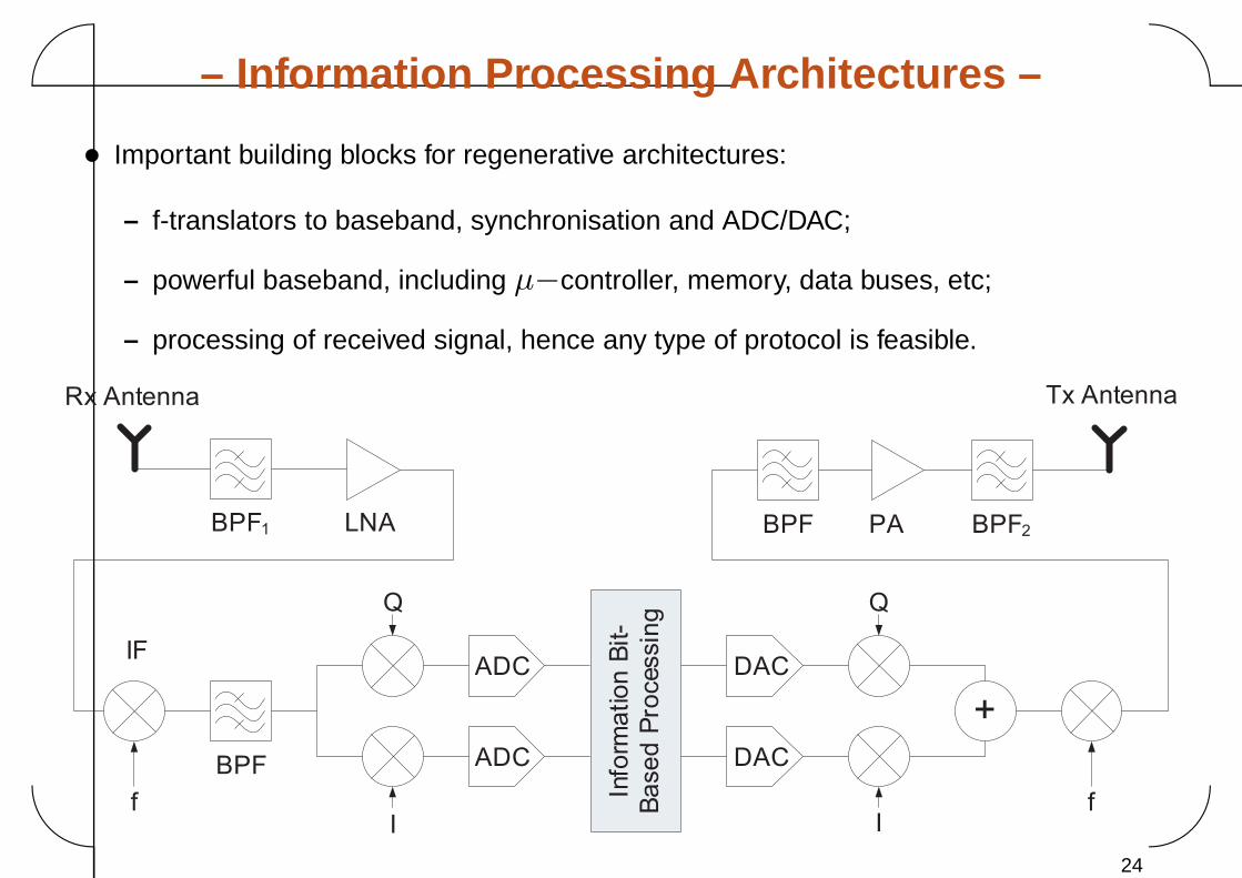
– Information Processing Architectures –

• Important building blocks for regenerative architectures:

– f-translators to baseband, synchronisation and ADC/DAC;

– powerful baseband, including μ−controller, memory, data buses, etc;

– processing of received signal, hence any type of protocol is feasible.

Rx Antenna

BPF1 LNA

IF

f

BPF PA BPF2

Tx Antenna

BPF

I

Q

ADC

ADC

DAC

DAC

I

Q

+

f

Info

rma

tio

n B

it-

Ba

se

d P

rocessin

g

24

�

�

�

�

Architectural Comparisons

25

�

�

�

�

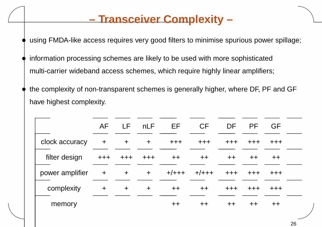
– Transceiver Complexity –

• using FMDA-like access requires very good filters to minimise spurious power spillage;

• information processing schemes are likely to be used with more sophisticated

multi-carrier wideband access schemes, which require highly linear amplifiers;

• the complexity of non-transparent schemes is generally higher, where DF, PF and GF

have highest complexity.

AF LF nLF EF CF DF PF GF

clock accuracy + + + +++ +++ +++ +++ +++

filter design +++ +++ +++ ++ ++ ++ ++ ++

power amplifier + + + +/+++ +/+++ +++ +++ +++

complexity + + + ++ ++ +++ +++ +++

memory ++ ++ ++ ++ ++

26

�

�

�

�

PART 3CHANNEL CHARACTERISATION

27

�

�

�

�

Regenerative Relaying Channel

28

�

�

�

�

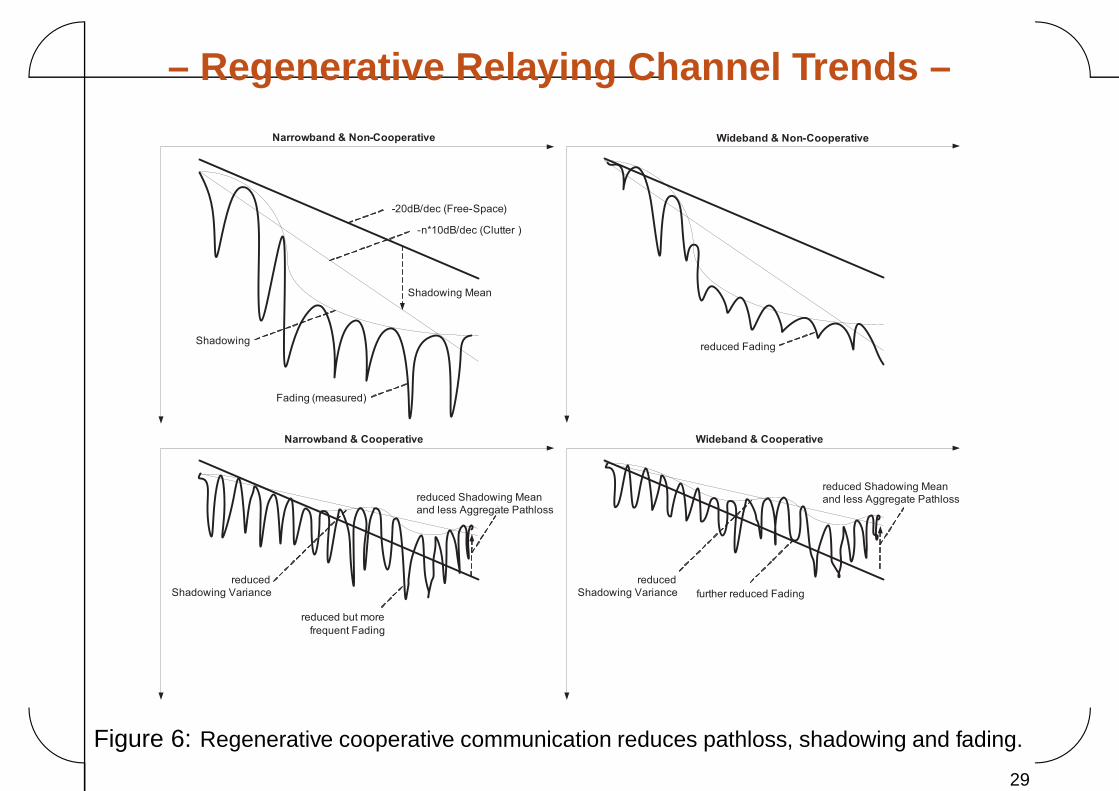
– Regenerative Relaying Channel Trends –

-20dB/dec (Free-Space)

-n*10dB/dec (Clutter )

Shadowing Mean

Shadowing

Fading (measured)

Narrowband & Non-Cooperative Wideband & Non-Cooperative

reduced Fading

Narrowband & Cooperative

reduced Shadowing Mean

and less Aggregate Pathloss

reduced

Shadowing Variance

Wideband & Cooperative

further reduced Fading

reduced Shadowing Mean

and less Aggregate Pathloss

reduced

Shadowing Variance

reduced but more

frequent Fading

Figure 6: Regenerative cooperative communication reduces pathloss, shadowing and fading.

29

�

�

�

�

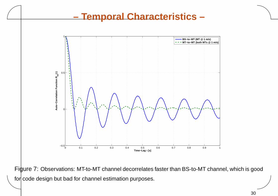
– Temporal Characteristics –

0 0.1 0.2 0.3 0.4 0.5 0.6 0.7 0.8 0.9 1−0.5

0

0.5

1

Time−Lag τ [s]

Au

to−C

orr

elat

ion

Fu

nct

ion

Rh

h(τ

)

BS−to−MT (MT @ 1 m/s)MT−to−MT (both MTs @ 1 m/s)

Figure 7: Observations: MT-to-MT channel decorrelates faster than BS-to-MT channel, which is good

for code design but bad for channel estimation purposes.

30

�

�

�

�

Transparent Relaying Channel

31

�

�

�

�

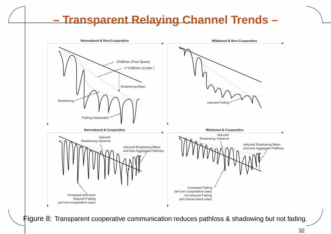
– Transparent Relaying Channel Trends –

-20dB/dec (Free-Space)

-n*10dB/dec (Clutter )

Shadowing Mean

Shadowing

Fading (measured)

Narrowband & Non-Cooperative Wideband & Non-Cooperative

reduced Fading

Narrowband & Cooperative

reduced Shadowing Mean

and less Aggregate Pathloss

reduced

Shadowing Variance

Wideband & Cooperative

reduced Shadowing Mean

and less Aggregate Pathloss

reduced

Shadowing Variance

increased and more

frequent Fading

(wrt non-cooperative case)

increased Fading

(wrt non-cooperative case)

but reduced Fading

(wrt narrow-band case)

Figure 8: Transparent cooperative communication reduces pathloss & shadowing but not fading.

32

�

�

�

�

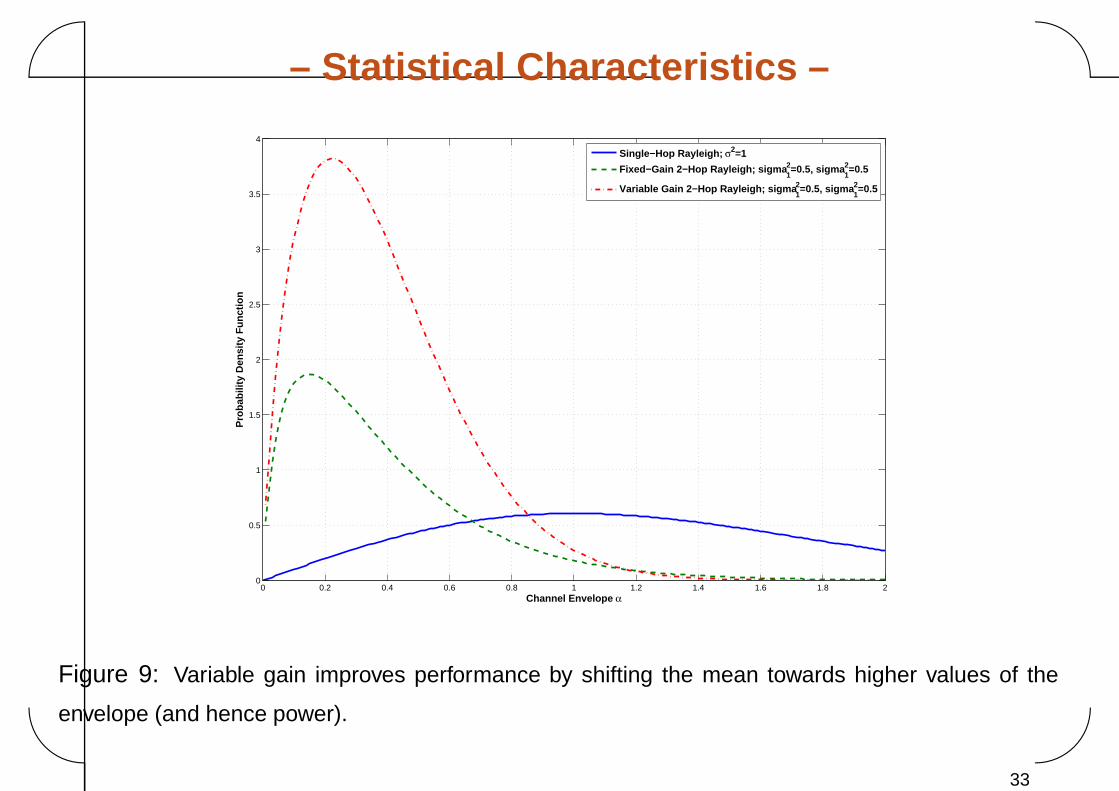
– Statistical Characteristics –

0 0.2 0.4 0.6 0.8 1 1.2 1.4 1.6 1.8 20

0.5

1

1.5

2

2.5

3

3.5

4

Channel Envelope α

Pro

bab

ility

Den

sity

Fu

nct

ion

Single−Hop Rayleigh; σ2=1

Fixed−Gain 2−Hop Rayleigh; sigma12=0.5, sigma

12=0.5

Variable Gain 2−Hop Rayleigh; sigma12=0.5, sigma

12=0.5

Figure 9: Variable gain improves performance by shifting the mean towards higher values of the

envelope (and hence power).

33

�

�

�

�

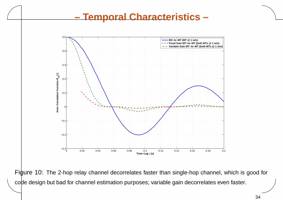
– Temporal Characteristics –

0 0.02 0.04 0.06 0.08 0.1 0.12 0.14 0.16 0.18 0.2−0.3

−0.2

−0.1

0

0.1

0.2

0.3

0.4

0.5

Time−Lag τ [s]

Au

to−C

orr

elat

ion

Fu

nct

ion

Rh

h(τ

)

BS−to−MT (MT @ 1 m/s)Fixed Gain MT−to−MT (both MTs @ 1 m/s)Variable Gain MT−to−MT (both MTs @ 1 m/s)

Figure 10: The 2-hop relay channel decorrelates faster than single-hop channel, which is good for

code design but bad for channel estimation purposes; variable gain decorrelates even faster.

34

�

�

�

�

Distributed MIMO Behaviour

35

�

�

�

�

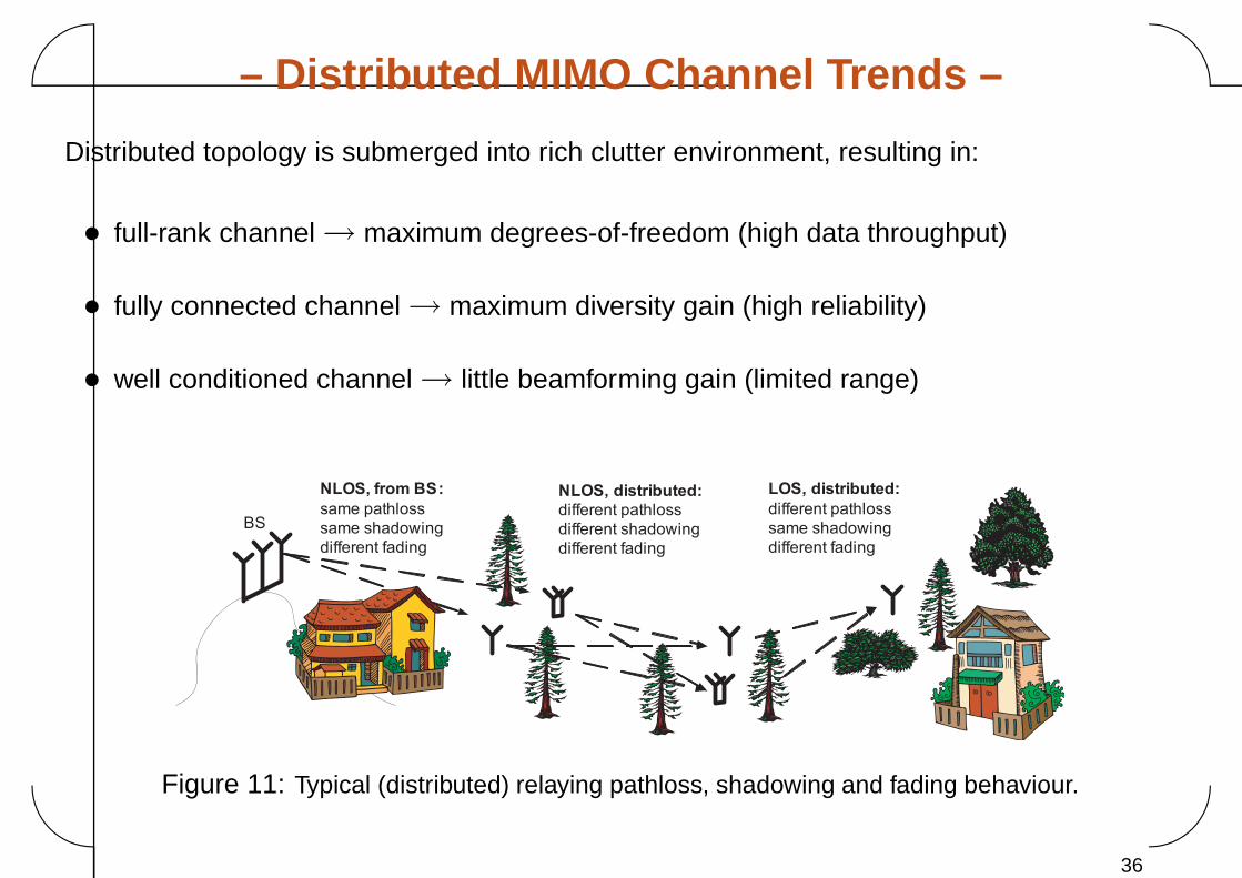
– Distributed MIMO Channel Trends –

Distributed topology is submerged into rich clutter environment, resulting in:

• full-rank channel → maximum degrees-of-freedom (high data throughput)

• fully connected channel → maximum diversity gain (high reliability)

• well conditioned channel → little beamforming gain (limited range)

NLOS, from BS:

same pathloss

same shadowing

different fading

NLOS, distributed:

different pathloss

different shadowing

different fading

LOS, distributed:

different pathloss

same shadowing

different fading

BS

Figure 11: Typical (distributed) relaying pathloss, shadowing and fading behaviour.

36

�

�

�

�

PART 4CSMA MAC & X-Layer Design

37

�

�

�

�

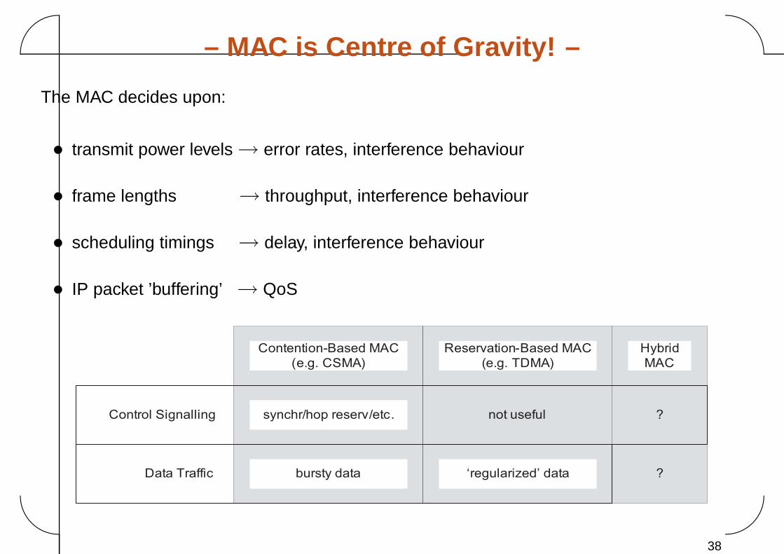
– MAC is Centre of Gravity! –

The MAC decides upon:

• transmit power levels → error rates, interference behaviour

• frame lengths → throughput, interference behaviour

• scheduling timings → delay, interference behaviour

• IP packet ’buffering’ → QoS

Contention-Based MAC

(e.g. CSMA)

Reservation-Based MAC

(e.g. TDMA)

Control Signalling

Data Traffic

synchr/hop reserv/etc. not useful

bursty data ‘regularized’ data

Hybrid

MAC

?

?

38

�

�

�

�

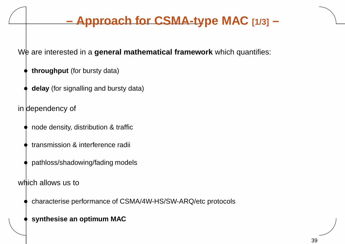
– Approach for CSMA-type MAC [1/3] –

We are interested in a general mathematical framework which quantifies:

• throughput (for bursty data)

• delay (for signalling and bursty data)

in dependency of

• node density, distribution & traffic

• transmission & interference radii

• pathloss/shadowing/fading models

which allows us to

• characterise performance of CSMA/4W-HS/SW-ARQ/etc protocols

• synthesise an optimum MAC

39

�

�

�

�

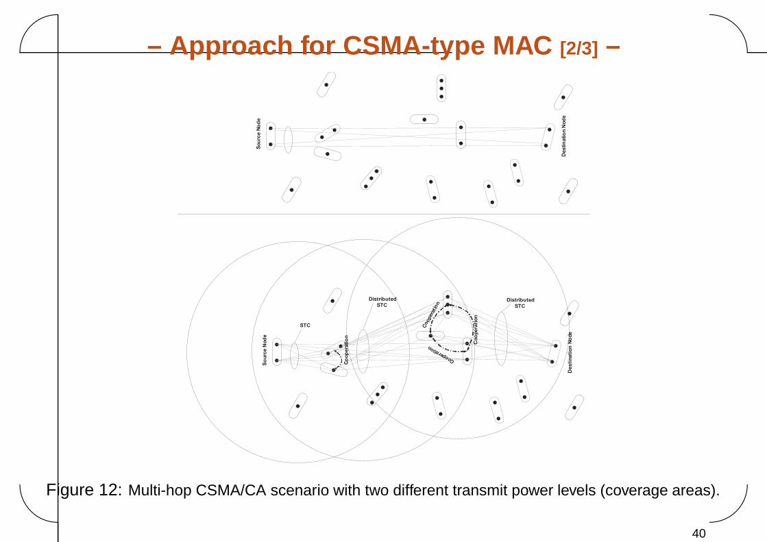
– Approach for CSMA-type MAC [2/3] –

Distributed

STC

Co

op

era

tio

n

So

urc

e N

od

e

Desti

nati

on

No

de

Coo

pera

tion

Coo

per

atio

n

Cooperation

Distributed

STC

STC

Sou

rce N

od

e

Destin

atio

n N

od

e

Figure 12: Multi-hop CSMA/CA scenario with two different transmit power levels (coverage areas).

40

�

�

�

�

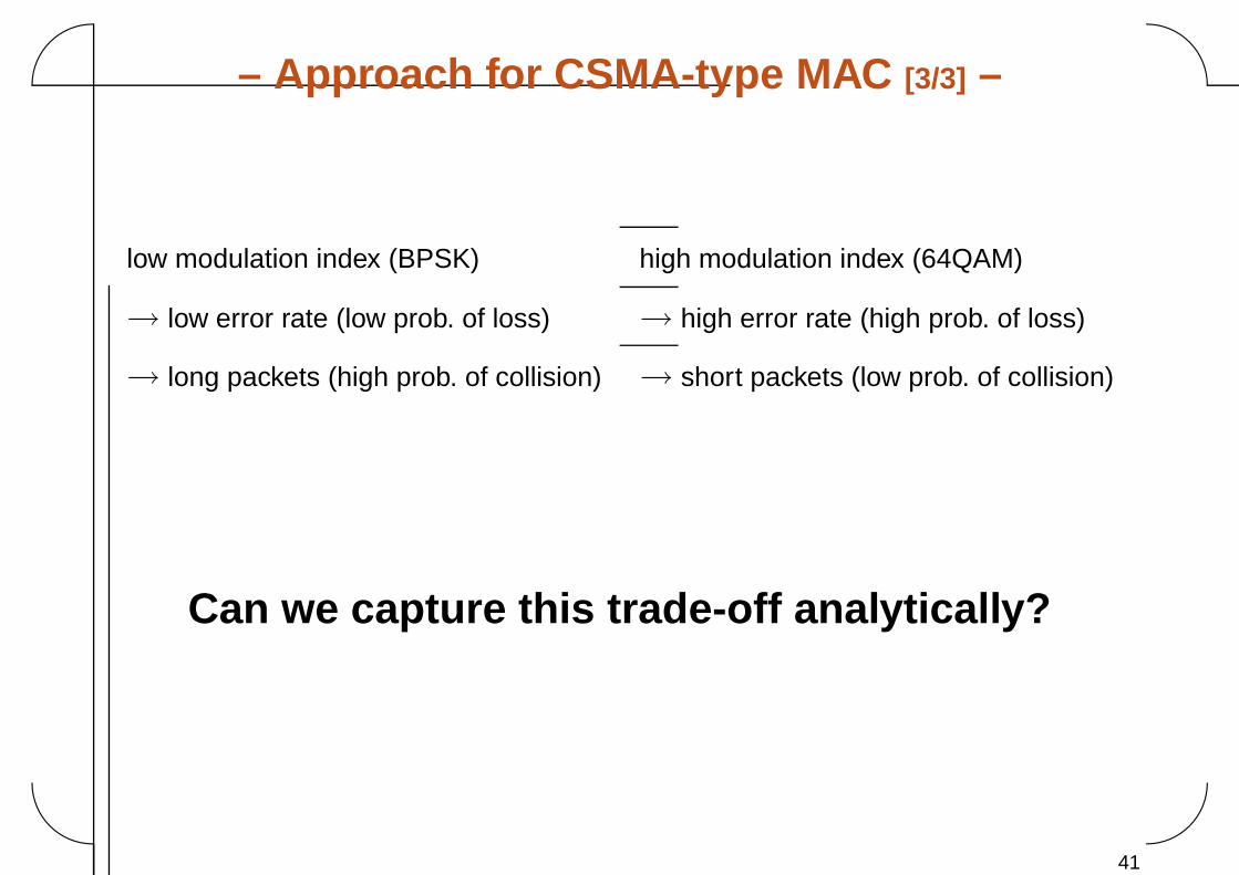
– Approach for CSMA-type MAC [3/3] –

low modulation index (BPSK) high modulation index (64QAM)

→ low error rate (low prob. of loss) → high error rate (high prob. of loss)

→ long packets (high prob. of collision) → short packets (low prob. of collision)

Can we capture this trade-off analytically?

41

�

�

�

�

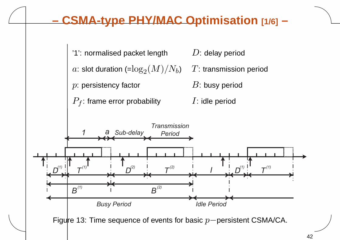
– CSMA-type PHY/MAC Optimisation [1/6] –

’1’: normalised packet length D: delay period

a: slot duration (=log2(M)/Nb) T : transmission period

p: persistency factor B: busy period

Pf : frame error probability I : idle period

D(1)

D(2)

D(1)

IT(1)

T(1)

T(2)

B(1)

B(2)

Busy Period Idle Period

a1 Sub-delayTransmission

Period

Figure 13: Time sequence of events for basic p−persistent CSMA/CA.

42

�

�

�

�

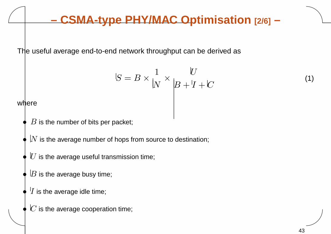
– CSMA-type PHY/MAC Optimisation [2/6] –

The useful average end-to-end network throughput can be derived as

S = B × 1N

× U

B + I + C(1)

where

• B is the number of bits per packet;

• N is the average number of hops from source to destination;

• U is the average useful transmission time;

• B is the average busy time;

• I is the average idle time;

• C is the average cooperation time;

43

�

�

�

�

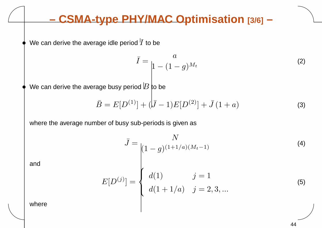
– CSMA-type PHY/MAC Optimisation [3/6] –

• We can derive the average idle period I to be

I =a

1 − (1 − g)Mt(2)

• We can derive the average busy period B to be

B = E[D(1)] + (J − 1)E[D(2)] + J (1 + a) (3)

where the average number of busy sub-periods is given as

J =N

(1 − g)(1+1/a)(Mt−1)(4)

and

E[D(j)] =

⎧⎨⎩

d(1) j = 1

d(1 + 1/a) j = 2, 3, ...(5)

where

44

�

�

�

�

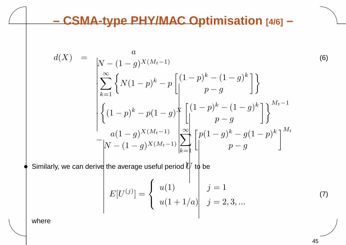
– CSMA-type PHY/MAC Optimisation [4/6] –

d(X) =a

N − (1 − g)X(Mt−1)(6)

·∞∑

k=1

{N(1 − p)k − p

[(1 − p)k − (1 − g)k

p − g

]}

·{

(1 − p)k − p(1 − g)X

[(1 − p)k − (1 − g)k

p − g

]}Mt−1

− a(1 − g)X(Mt−1)

N − (1 − g)X(Mt−1)

∞∑k=1

[p(1 − g)k − g(1 − p)k

p − g

]Mt

• Similarly, we can derive the average useful period U to be

E[U (j)] =

⎧⎨⎩

u(1) j = 1

u(1 + 1/a) j = 2, 3, ...(7)

where

45

�

�

�

�

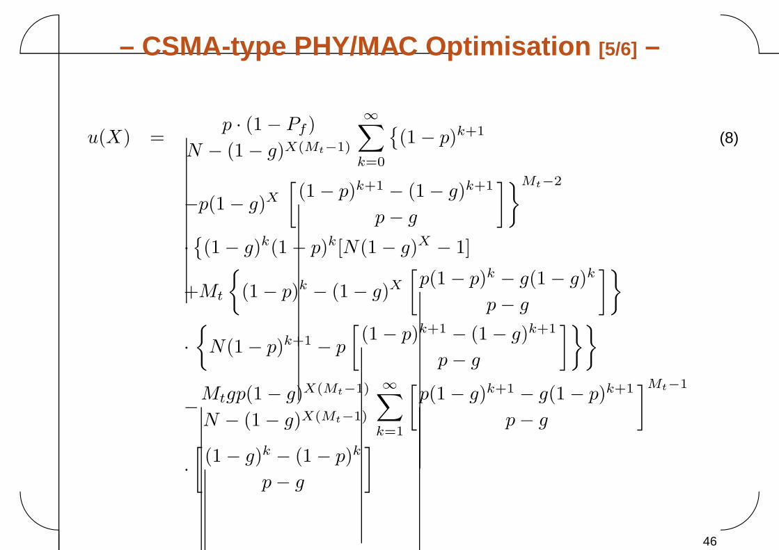
– CSMA-type PHY/MAC Optimisation [5/6] –

u(X) =p · (1 − Pf )

N − (1 − g)X(Mt−1)

∞∑k=0

{(1 − p)k+1 (8)

−p(1 − g)X

[(1 − p)k+1 − (1 − g)k+1

p − g

]}Mt−2

·{(1 − g)k(1 − p)k[N(1 − g)X − 1]

+Mt

{(1 − p)k − (1 − g)X

[p(1 − p)k − g(1 − g)k

p − g

]}

·{

N(1 − p)k+1 − p

[(1 − p)k+1 − (1 − g)k+1

p − g

]}}

−Mtgp(1 − g)X(Mt−1)

N − (1 − g)X(Mt−1)

∞∑k=1

[p(1 − g)k+1 − g(1 − p)k+1

p − g

]Mt−1

·[(1 − g)k − (1 − p)k

p − g

]

46

�

�

�

�

– CSMA-type PHY/MAC Optimisation [6/6] –

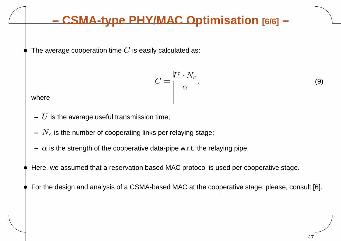
• The average cooperation time C is easily calculated as:

C =U · Nc

α, (9)

where

– U is the average useful transmission time;

– Nc is the number of cooperating links per relaying stage;

– α is the strength of the cooperative data-pipe w.r.t. the relaying pipe.

• Here, we assumed that a reservation based MAC protocol is used per cooperative stage.

• For the design and analysis of a CSMA-based MAC at the cooperative stage, please, consult [6].

47

�

�

�

�

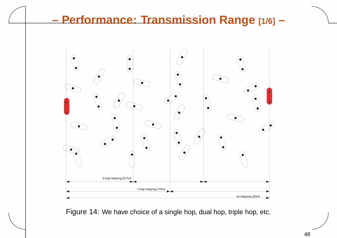
– Performance: Transmission Range [1/6] –

no relaying (20m)

1-hop relaying (10m)

2-hop relaying (6.7m)

Figure 14: We have choice of a single hop, dual hop, triple hop, etc.

48

�

�

�

�

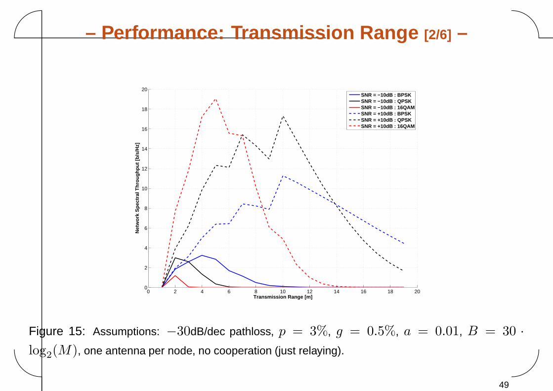
– Performance: Transmission Range [2/6] –

0 2 4 6 8 10 12 14 16 18 200

2

4

6

8

10

12

14

16

18

20

Transmission Range [m]

Net

wo

rk S

pec

tral

Th

rou

gh

pu

t [b

/s/H

z]

SNR = −10dB : BPSKSNR = −10dB : QPSKSNR = −10dB : 16QAMSNR = +10dB : BPSKSNR = +10dB : QPSKSNR = +10dB : 16QAM

Figure 15: Assumptions: −30dB/dec pathloss, p = 3%, g = 0.5%, a = 0.01, B = 30 ·log2(M), one antenna per node, no cooperation (just relaying).

49

�

�

�

�

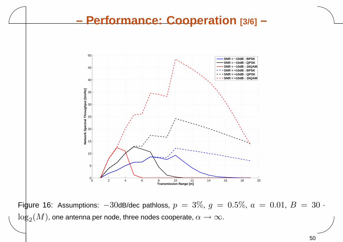
– Performance: Cooperation [3/6] –

0 2 4 6 8 10 12 14 16 18 200

5

10

15

20

25

30

35

40

45

50

Transmission Range [m]

Net

wo

rk S

pec

tral

Th

rou

gh

pu

t [b

/s/H

z]

SNR = −10dB : BPSKSNR = −10dB : QPSKSNR = −10dB : 16QAMSNR = +10dB : BPSKSNR = +10dB : QPSKSNR = +10dB : 16QAM

Figure 16: Assumptions: −30dB/dec pathloss, p = 3%, g = 0.5%, a = 0.01, B = 30 ·log2(M), one antenna per node, three nodes cooperate, α → ∞.

50

�

�

�

�

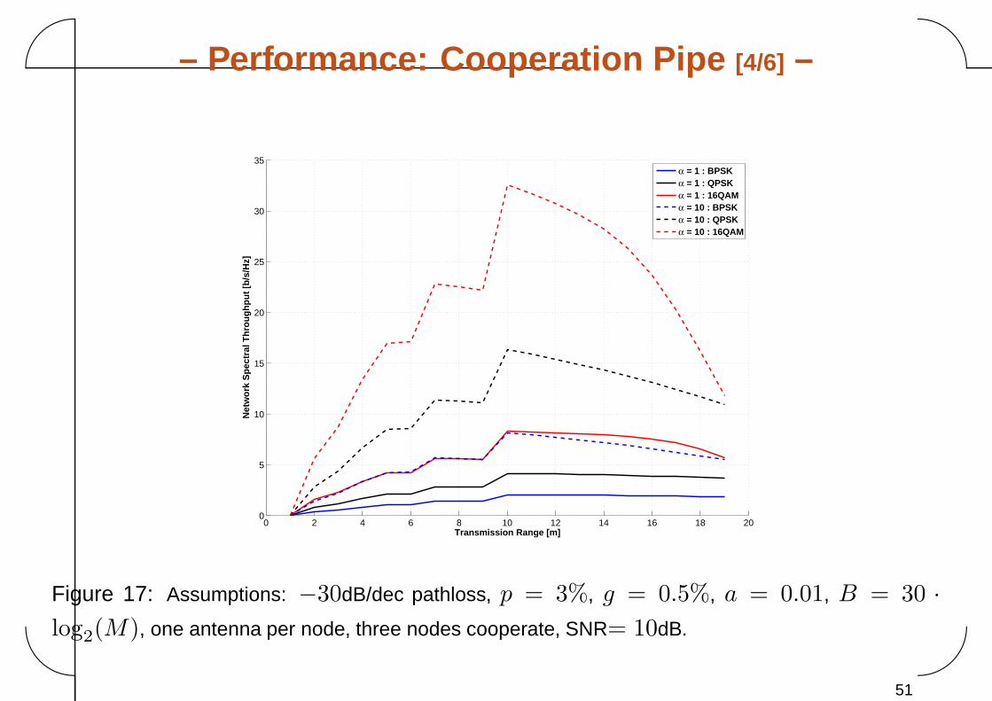
– Performance: Cooperation Pipe [4/6] –

0 2 4 6 8 10 12 14 16 18 200

5

10

15

20

25

30

35

Transmission Range [m]

Net

wo

rk S

pec

tral

Th

rou

gh

pu

t [b

/s/H

z]

α = 1 : BPSKα = 1 : QPSKα = 1 : 16QAMα = 10 : BPSKα = 10 : QPSKα = 10 : 16QAM

Figure 17: Assumptions: −30dB/dec pathloss, p = 3%, g = 0.5%, a = 0.01, B = 30 ·log2(M), one antenna per node, three nodes cooperate, SNR= 10dB.

51

�

�

�

�

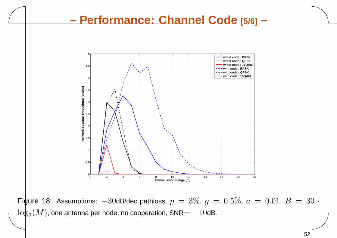
– Performance: Channel Code [5/6] –

0 2 4 6 8 10 12 14 16 18 200

0.5

1

1.5

2

2.5

3

3.5

4

4.5

5

Transmission Range [m]

Net

wo

rk S

pec

tral

Th

rou

gh

pu

t [b

/s/H

z]

w/out code : BPSKw/out code : QPSKw/out code : 16QAMwith code : BPSKwith code : QPSKwith code : 16QAM

Figure 18: Assumptions: −30dB/dec pathloss, p = 3%, g = 0.5%, a = 0.01, B = 30 ·log2(M), one antenna per node, no cooperation, SNR= −10dB.

52

�

�

�

�

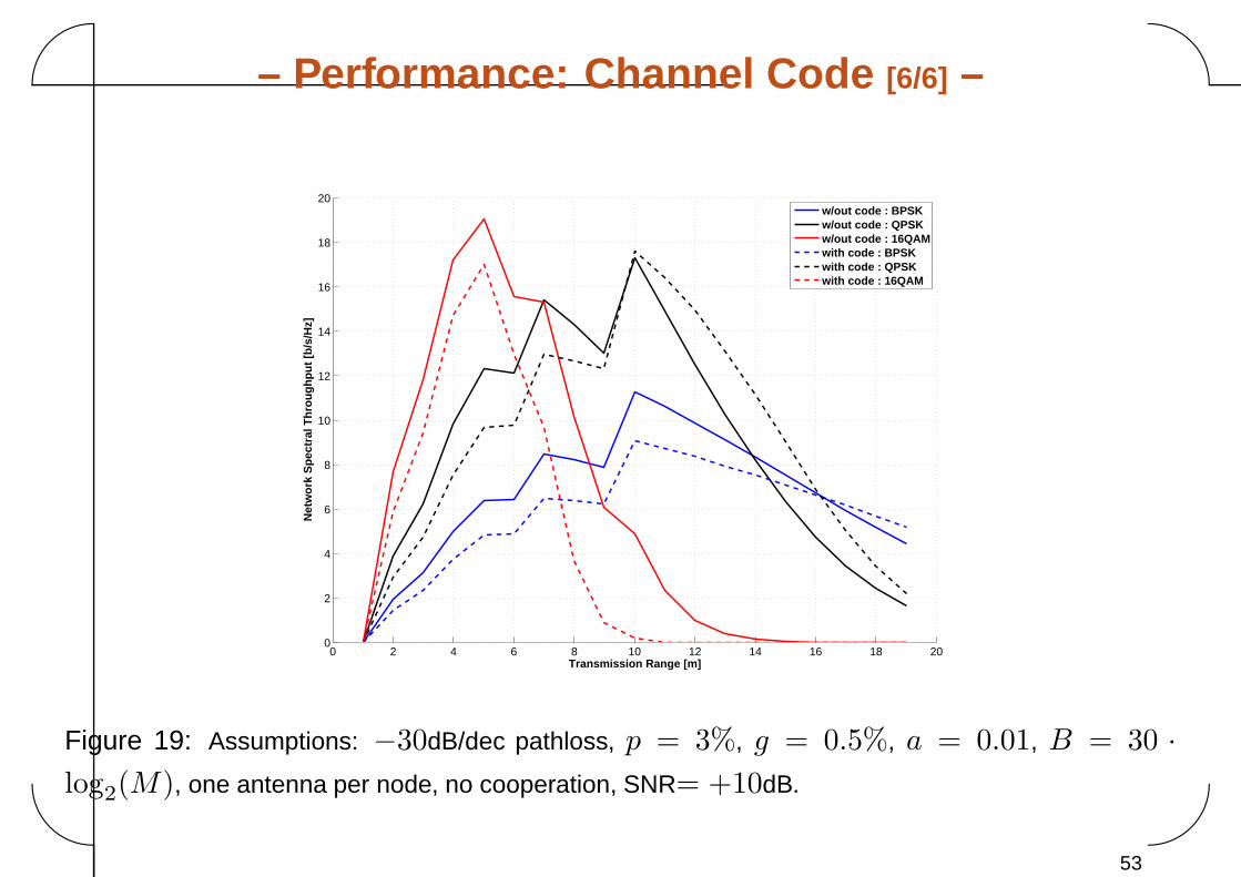
– Performance: Channel Code [6/6] –

0 2 4 6 8 10 12 14 16 18 200

2

4

6

8

10

12

14

16

18

20

Transmission Range [m]

Net

wo

rk S

pec

tral

Th

rou

gh

pu

t [b

/s/H

z]

w/out code : BPSKw/out code : QPSKw/out code : 16QAMwith code : BPSKwith code : QPSKwith code : 16QAM

Figure 19: Assumptions: −30dB/dec pathloss, p = 3%, g = 0.5%, a = 0.01, B = 30 ·log2(M), one antenna per node, no cooperation, SNR= +10dB.

53

�

�

�

�

PART 5CONCLUSIONS & ROAD AHEAD

54

�

�

�

�

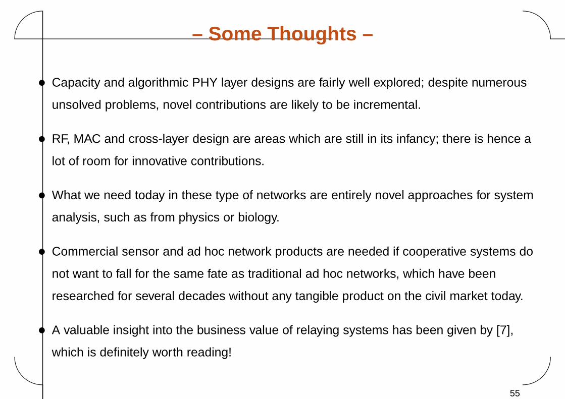
– Some Thoughts –

• Capacity and algorithmic PHY layer designs are fairly well explored; despite numerous

unsolved problems, novel contributions are likely to be incremental.

• RF, MAC and cross-layer design are areas which are still in its infancy; there is hence a

lot of room for innovative contributions.

• What we need today in these type of networks are entirely novel approaches for system

analysis, such as from physics or biology.

• Commercial sensor and ad hoc network products are needed if cooperative systems do

not want to fall for the same fate as traditional ad hoc networks, which have been

researched for several decades without any tangible product on the civil market today.

• A valuable insight into the business value of relaying systems has been given by [7],

which is definitely worth reading!

55

�

�

�

�

REFERENCES

56

REFERENCES�

�

�

�

References

[1] 3G TR 25.924 V1.0.0 (1999-12) 3rd Generation Partnership Project, Technical Specification Group Radio Access

Network; Opportunity Driven Multiple Access.

[2] N. Esseling, E. Weiss, A. Krmling, W. Zirwas, “A Multi Hop Concept for HiperLAN/2: Capacity and Interference,” Proc.

European Wireless 2002 , Vol. 1, pp. 1-7, Florence, Italy, February 2002.

[3] I.F. Akyildiz, W. Su, Y. Sankarasubramaniam, E. Cayirci, “Wireless Sensor Networks: A Survey,” Computer Networks,

34(4):393-422, March 2002.

[4] R.C. Palat, A. Annamalai, J.H. Reed, “Cooperative Relaying for Ad-Hoc Ground Networks using Swarm UAVs,” Milcom

2005, Atlantic City, New Jersey, October 2005.

[5] M. Dohler, Virtual Antenna Arrays, PhD Thesis, University of London, King’s College London, London, UK, 2003.

[6] J. Alonso-Zarate, J. Gomez, C. Verikoukis, L. Alonso, A. Perez-Neira, “Performance Evaluation of a Cooperative

Scheme for Wireless Networks,” IEEE PIMRC 2006, September 2006, Conference CD-ROM, Helsinki, Finland.

[7] B. Timus, Deployment Cost Efficiency in Broadband Delivery with Fixed Wireless Relays, Licentiate Thesis, KTH,

Sweden, 2006.

57