Embed Size (px)
DESCRIPTION
Multi input Multi output systems
Citation preview
1 | Finding MIMO – Charan Langton – www.complextoreal.com
Tutorial 27 - Finding MIMO
Charan Langton, Bernard Sklar
Oct 2011
When multiple input/multiple output (MIMO) systems were described in the mid-to-late 1990s by
Gerard Foschini and others, [1] the astonishing bandwidth efficiency of such techniques seemed
to be in violation of the Shannon limit. But, there is no violation because the diversity and signal
processing employed with MIMO transforms a point-to-point single channel into multiple parallel
or matrix channels, hence in effect multiplying the capacity. MIMO offers higher data rates as
well as spectral efficiency. So clear is this advantage that many standards have already
incorporated MIMO. ITU uses MIMO in the High Speed Downlink Packet Access (HSPDA),
part of the UMTS standard. MIMO is also part of the 802.11n standard used by your wireless
router as well as 802.16 for Mobile WiMax used by your cell phone. The LTE standard also
incorporates MIMO.
What is MIMO as compared to a traditional communications channel? A traditional
communications link, which we call a single-in-single-out (SISO) channel, has one transmitter
and one receiver. But instead of a single transmitter and a single receiver we can use several of
each. The SISO channel then becomes a multiple-in-multiple-out, or a MIMO channel; i.e. a
channel that has multiple transmitters and multiple receivers.
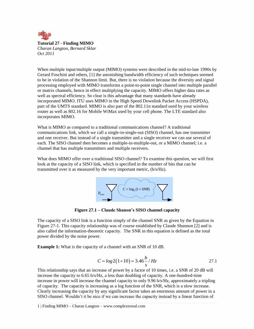
What does MIMO offer over a traditional SISO channel? To examine this question, we will first
look at the capacity of a SISO link, which is specified in the number of bits that can be
transmitted over it as measured by the very important metric, (b/s/Hz).
2log (1 )C SNR
TotalP
Figure 27.1 – Claude Shanon’s SISO channel capacity
The capacity of a SISO link is a function simply of the channel SNR as given by the Equation in
Figure 27-1. This capacity relationship was of course established by Claude Shannon [2] and is
also called the information-theoretic capacity. The SNR in this equation is defined as the total
power divided by the noise power.
Example 1: What is the capacity of a channel with an SNR of 10 dB.
2 1 10 3.46 /b
C log Hzs
27.1
This relationship says that an increase of power by a factor of 10 times, i.e. a SNR of 20 dB will
increase the capacity to 6.65 b/s/Hz, a less than doubling of capacity. A one-hundred-time
increase in power will increase the channel capacity to only 9.96 b/s/Hz, approximately a tripling
of capacity. The capacity is increasing as a log function of the SNR, which is a slow increase.
Clearly increasing the capacity by any significant factor takes an enormous amount of power in a
SISO channel. Wouldn’t it be nice if we can increase the capacity instead by a linear function of
2 | Finding MIMO – Charan Langton – www.complextoreal.com
power; 10 times increase in power, 10 times increase in capacity! Perhaps we can do this with
MIMO.
With MIMO, we move to a different paradigm of channel capacity. To give you a feel for what is
possible, if we add six antennas on both transmit and receive side, we can achieve the same
capacity as using 100 times more power than in the SISO case. So what did we do here? We just
made the transmitter and receiver more complex, with no increase in power at all. We got the
same performance as increasing the power 100 times. Quite amazing, and worth examining
closely.
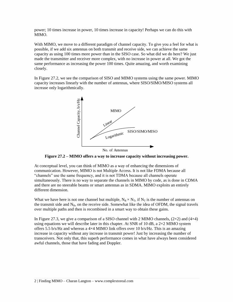
In Figure 27.2, we see the comparison of SISO and MIMO systems using the same power. MIMO
capacity increases linearly with the number of antennas, where SISO/SIMO/MISO systems all
increase only logarithmically.
MIMO
SISO/SIMO/MISO
Linear
Logarithmic
No. of Antennas
Ch
ann
el C
apac
ity, b
/s/H
z
Figure 27.2 – MIMO offers a way to increase capacity without increasing power.
At conceptual level, you can think of MIMO as a way of enhancing the dimensions of
communication. However, MIMO is not Multiple Access. It is not like FDMA because all
“channels” use the same frequency, and it is not TDMA because all channels operate
simultaneously. There is no way to separate the channels in MIMO by code, as is done in CDMA
and there are no steerable beams or smart antennas as in SDMA. MIMO exploits an entirely
different dimension.
What we have here is not one channel but multiple, NR × NT, if NT is the number of antennas on
the transmit side and NR, on the receive side. Somewhat like the idea of OFDM, the signal travels
over multiple paths and then is recombined in a smart way to obtain these gains.
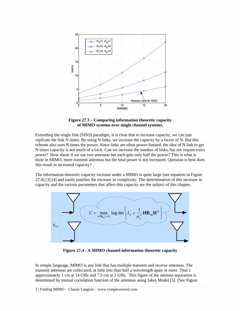
In Figure 27.3, we give a comparison of a SISO channel with 2 MIMO channels, (2×2) and (4×4)
using equations we will describe later in this chapter. At SNR of 10 dB, a 2×2 MIMO system
offers 5.5 b/s/Hz and whereas a 4×4 MIMO link offers over 10 b/s/Hz. This is an amazing
increase in capacity without any increase in transmit power! Just by increasing the number of
transceivers. Not only that, this superb performance comes in what have always been considered
awful channels, those that have fading and Doppler.
3 | Finding MIMO – Charan Langton – www.complextoreal.com
Figure 27.3 – Comparing information theoretic capacity
of MIMO systems over single channel systems.
Extending the single link (SISO) paradigm, it is clear that to increase capacity, we can just
replicate the link N times. By using N links, we increase the capacity by a factor of N. But this
scheme also uses N times the power. Since links are often power-limited, the idea of N link to get
N times capacity is not much of a trick. Can we increase the number of links, but not require extra
power? How about if we use two antennas but each gets only half the power? This is what is
done in MIMO, more transmit antennas but the total power is not increased. Question is how does
this result in increased capacity?
The information-theoretic capacity increase under a MIMO is quite large (see equation in Figure
27.4) [3] [4] and easily justifies the increase in complexity. The determination of this increase in
capacity and the various parameters that affect this capacity are the subject of this chapter.
2( )
1max log det
T
H
Ntr P
n
C I
xx
xxR
HR H
TotalP
Figure 27.4 - A MIMO channel information theoretic capacity
In simple language, MIMO is any link that has multiple transmit and receive antennas. The
transmit antennas are collocated, at little less than half a wavelength apart or more. That’s
approximately 1 cm at 14 GHz and 7.5 cm at 2 GHz. This figure of the antenna separation is
determined by mutual correlation function of the antennas using Jakes Model [5]. (See Figure
4 | Finding MIMO – Charan Langton – www.complextoreal.com
27.16)The receive antennas are also part of one unit. Just as in SISO links, the communication is
assumed to be between one sender and one receiver, although MIMO is also used in multi-user
scenario, similar in the way OFDM can be used for one or multiple users.
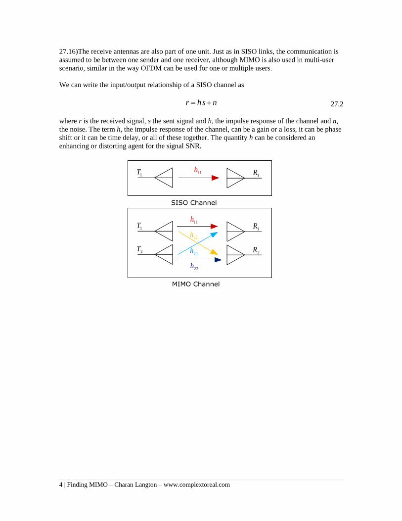
We can write the input/output relationship of a SISO channel as
r h s n 27.2
where r is the received signal, s the sent signal and h, the impulse response of the channel and n,
the noise. The term h, the impulse response of the channel, can be a gain or a loss, it can be phase
shift or it can be time delay, or all of these together. The quantity h can be considered an
enhancing or distorting agent for the signal SNR.
11h
12h
22h
21h2T
1T
2R
1R
11h1T
1R
5 | Finding MIMO – Charan Langton – www.complextoreal.com
11h
12h1T
2R
1R
11h
21h2T
1T1R
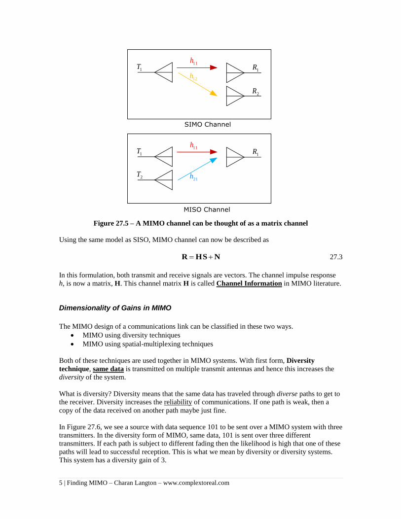
Figure 27.5 – A MIMO channel can be thought of as a matrix channel
Using the same model as SISO, MIMO channel can now be described as
R HS N 27.3
In this formulation, both transmit and receive signals are vectors. The channel impulse response
h, is now a matrix, H. This channel matrix H is called Channel Information in MIMO literature.
Dimensionality of Gains in MIMO
The MIMO design of a communications link can be classified in these two ways.
MIMO using diversity techniques
MIMO using spatial-multiplexing techniques
Both of these techniques are used together in MIMO systems. With first form, Diversity
technique, same data is transmitted on multiple transmit antennas and hence this increases the
diversity of the system.
What is diversity? Diversity means that the same data has traveled through diverse paths to get to
the receiver. Diversity increases the reliability of communications. If one path is weak, then a
copy of the data received on another path maybe just fine.
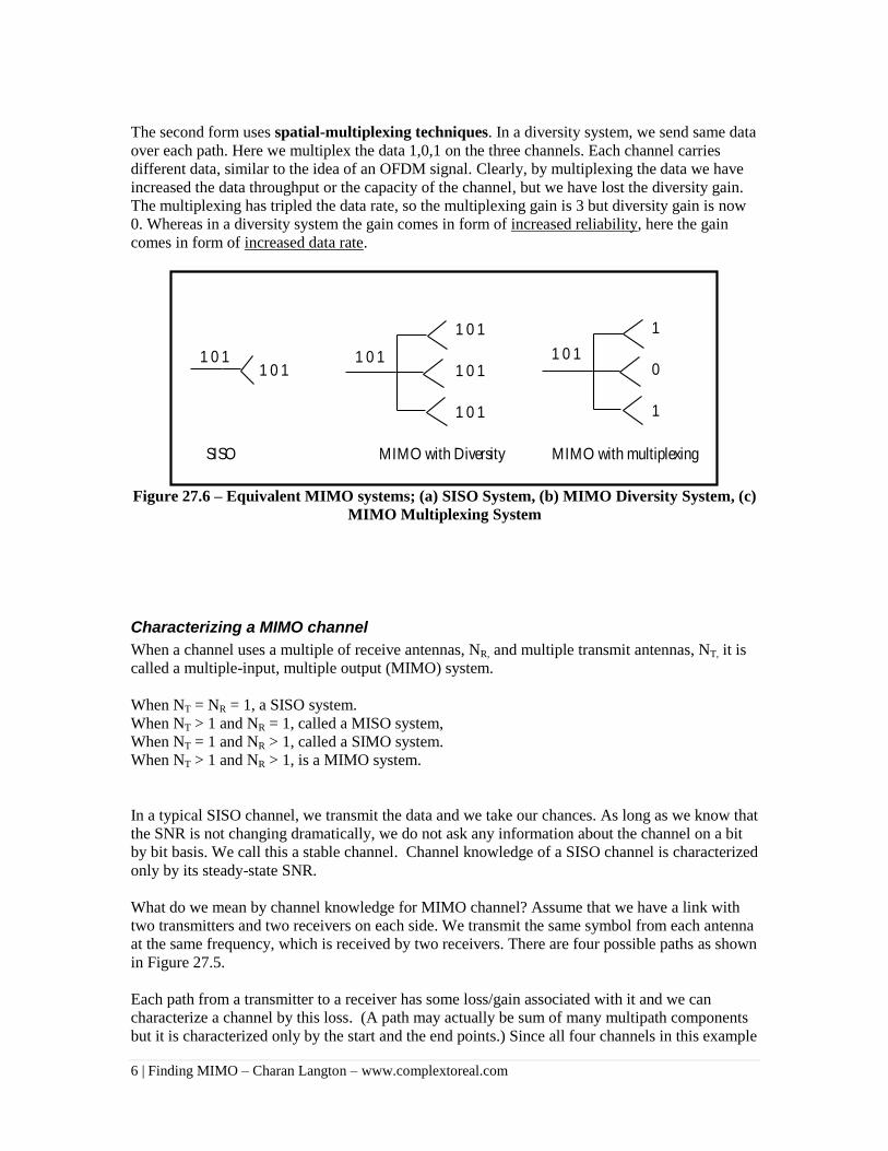
In Figure 27.6, we see a source with data sequence 101 to be sent over a MIMO system with three
transmitters. In the diversity form of MIMO, same data, 101 is sent over three different
transmitters. If each path is subject to different fading then the likelihood is high that one of these
paths will lead to successful reception. This is what we mean by diversity or diversity systems.
This system has a diversity gain of 3.
6 | Finding MIMO – Charan Langton – www.complextoreal.com
The second form uses spatial-multiplexing techniques. In a diversity system, we send same data
over each path. Here we multiplex the data 1,0,1 on the three channels. Each channel carries
different data, similar to the idea of an OFDM signal. Clearly, by multiplexing the data we have
increased the data throughput or the capacity of the channel, but we have lost the diversity gain.
The multiplexing has tripled the data rate, so the multiplexing gain is 3 but diversity gain is now
0. Whereas in a diversity system the gain comes in form of increased reliability, here the gain
comes in form of increased data rate.
Figure 27.6 – Equivalent MIMO systems; (a) SISO System, (b) MIMO Diversity System, (c)
MIMO Multiplexing System
Characterizing a MIMO channel
When a channel uses a multiple of receive antennas, NR, and multiple transmit antennas, NT, it is
called a multiple-input, multiple output (MIMO) system.
When NT = NR = 1, a SISO system.
When NT > 1 and NR = 1, called a MISO system,
When NT = 1 and NR > 1, called a SIMO system.
When NT > 1 and NR > 1, is a MIMO system.
In a typical SISO channel, we transmit the data and we take our chances. As long as we know that
the SNR is not changing dramatically, we do not ask any information about the channel on a bit
by bit basis. We call this a stable channel. Channel knowledge of a SISO channel is characterized
only by its steady-state SNR.
What do we mean by channel knowledge for MIMO channel? Assume that we have a link with
two transmitters and two receivers on each side. We transmit the same symbol from each antenna
at the same frequency, which is received by two receivers. There are four possible paths as shown
in Figure 27.5.
Each path from a transmitter to a receiver has some loss/gain associated with it and we can
characterize a channel by this loss. (A path may actually be sum of many multipath components
but it is characterized only by the start and the end points.) Since all four channels in this example
1 0 1
1 0 1
1 0 1
1 0 1
1 0 1
1
0
1
1 0 11 0 1
SISO MIMO with Diversity MIMO with multiplexing
7 | Finding MIMO – Charan Langton – www.complextoreal.com
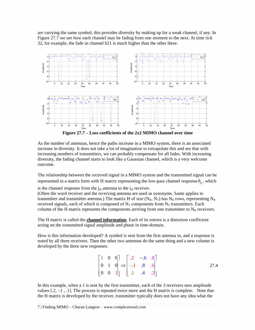
are carrying the same symbol, this provides diversity by making up for a weak channel, if any. In
Figure 27.7 we see how each channel may be fading from one moment to the next. At time tick
32, for example, the fade in channel h21 is much higher than the other three.
Figure 27.7 – Loss coefficients of the 2x2 MIMO channel over time
As the number of antennas, hence the paths increase in a MIMO system, there is an associated
increase in diversity. It does not take a lot of imagination to extrapolate this and see that with
increasing numbers of transmitters, we can probably compensate for all fades. With increasing
diversity, the fading channel starts to look like a Gaussian channel, which is a very welcome
outcome.
The relationship between the received signal in a MIMO system and the transmitted signal can be
represented in a matrix form with H matrix representing the low-pass channel response ijh , which
is the channel response from the jth antenna to the ith receiver.
(Often the word receiver and the receiving antenna are used as synonyms. Same applies to
transmitter and transmitter antenna.) The matrix H of size (NR, NT) has NR rows, representing NR
received signals, each of which is composed of NT components from NT transmitters. Each
column of the H matrix represents the components arriving from one transmitter to NR receivers.
The H matrix is called the channel information. Each of its entries is a distortion coefficient
acting on the transmitted signal amplitude and phase in time-domain.
How is this information developed? A symbol is sent from the first antenna in, and a response is
noted by all three receivers. Then the other two antennas do the same thing and a new column is
developed by the three new responses.
.1 80 0
.0 0
.6
1 .8
.2
.1
.1 .10
6
4 .20
27.4
In this example, when a 1 is sent by the first transmitter, each of the 3 receivers sees amplitude
values [.2, -.1 , .1]. The process is repeated twice more and the H matrix is complete. Note that
the H matrix is developed by the receiver, transmitter typically does not have any idea what the
5 10 15 20 25 30 35 40 45 50-10
-8
-6
-4
-2
0
Time
Am
plitu
de
h11
5 10 15 20 25 30 35 40 45 50-10
-8
-6
-4
-2
0
Time
Am
plitu
de
h12
5 10 15 20 25 30 35 40 45 50-10
-8
-6
-4
-2
0
Time
Am
plitu
de
h21
5 10 15 20 25 30 35 40 45 50-10
-8
-6
-4
-2
0
Time
Am
plitu
de
h22

8 | Finding MIMO – Charan Langton – www.complextoreal.com
channel looks like. It is transmitting blindly. If the receiver then turns around and transmits this
matrix back to the transmitter, then the transmitter would be able to see how the signals are faring
and might want to make adjustments in the powers allocated to its antennas. Perhaps a smart
computer at the transmitter will decide to not transmit on antenna 1, since the received signals are
so much smaller (in amplitude) than the other two antennas. Maybe we should just split the power
between antenna 2 and 3 and turn off antenna 1 until the channel improves. This is a good idea
and that’s just what is done.
The following shows two examples of an H matrix, the first with only amplitude changes and the
second with complex entries that include both amplitude and phase changes which is a more
realistic scenario.
0.8 0.5 0.3 0.8 0.5 0.2 0.3 0.6
0.4 1.0 0.2 0.4 0.6 1.0 0.1 0.2 0.9
0.5 0.5 0.6 0.5 0.3 0.5 1.5 0.6 1.2
j j
j j j
j j j
27.5
Modeling a MIMO Channel
We start with a general channel which has both multipath and Doppler (the conditions facing a
mobile in case of a cell phone system). The channel matrix H for this channel takes this form.
11 12 1
21 22 2
,1 ,2
( , ) ( , ) ( , )
( , ) ( , ) ( , )( , )
( , ) ( , ) ( , )
T
T
R R R T
N
N
N N N N
h t h t h t
h t h t h tH t
h t h t h t
27.6
Each path coefficient is a function of not only time t because the mobile is moving but also a time
delay relative to other paths. The variable indicates relative delays between each component
caused by frequency shifts. The time variable t represents the time-varying nature of the channel
such as one that has Doppler or other time variations. [6]
If the transmitted signal is si(t), and the received signal is ri(t), we write the input-output
relationship of a general MIMO channel as
1
1
( ) ( , ) ( )
( , ) ( ) 1,2
T
T
N
i ij j
j
N
ij j R
j
r t h t s t d
h t s i N
27.7
The channel equation for the received signal ri(t) is expressed as convolution of the channel
matrix H and the transmitted signals because of the delay variable . We write this relationship
in matrix form as
( ) ( , ) ( )t t t r H s 27.8
9 | Finding MIMO – Charan Langton – www.complextoreal.com
If we assume that the channel is flat (non-frequency selective), but is time-varying, i.e. has
Doppler, we would write this relationship without the convolution as
( ) ( ) ( )t t tr H s 27.9
In this case, the H matrix changes randomly with time. If the time variations are very slow (non-
moving receiver and transmitter) such that during a block of transmission longer than the several
symbols, we can assume the channel to be non-varying, or static. A fixed realization of the H
matrix can be written as follows (27.11). The individual entries can be either scalar or complex.
For analysis purposes, we can make some important assumptions about the H matrix. We can
assume that it is fixed for a period of one or more symbols and then changes randomly. This is a
fast change and causes the SNR of the received signal to change very rapidly. Or we can assume
that it is fixed for a block of time, such as over a full code sequence, which makes decoding
easier because the decoder does not have to deal with a variable SNR over a block. Or we can
assume that the channel is semi-static such as in a TDMA system, and its behavior is static over a
burst or more. Each version of the H matrix seen is called its realization. How fast these
realizations change depends on the channel type.
11 12 1
21 22 2
,1 ,2
T
T
R R R T
N
N
N N N N
h h h
h h h
h h h
H 27.10
For a fixed random realization of the H matrix, the input-output relationship can be written
without the convolution as
( ) ( )t tr H s 27.11
In this channel model, the H matrix is assumed fixed. An example of this type of situation where
the H matrix may remain fixed for a long period would be a phone call taking place from one
fixed place to another. In most cases, we can consider the channel to be static. This allows us to
treat the channel as deterministic over that period and amenable to analysis.
The power received at all receive antennas is equal to the sum of the total transmit power,
assuming channel offers no gain or loss. Each entry hij is an amplitude and phase term. Squaring
it give us the power for that path. There are NT paths to each receiver, so the sum of j terms, gives
us the total transmit power. Each receiver receives the total transmit power. For this relation we
have assumed that the transmit power of each transmitter is 1.0.
2
1
TN
ij T
j
h N
27.12
The H matrix is a very important construct in understanding MIMO capacity and performance.
How a MIMO system performs depends on the condition of the channel matrix H and its
properties. The H matrix can be thought of as a set of simultaneous equations. Each equation
10 | Finding MIMO – Charan Langton – www.complextoreal.com
represents a received signal which is a composite of unique set of channel coefficients applied to
the transmitted signal.
1 11 12 1 TNr h s h s h s 27.13
If the number of transmitters is equal to the number of receivers, then there exists a unique
solution to these equations. If the number of equations is larger than the number of unknowns (
i.e. NR > NT) then the solution can be found using a zero-forcing algorithm. When NT = NR, then
the solution can be found by (ignoring noise) inverting the H matrix as in
1( ) ( )s t H r t 27.14
The system performs best when the H matrix is full rank, with each row/column meeting
conditions of independence. What this means is that best performance is achieved only when each
path is fully independent of all others. This can happen only in an environment that offers rich
scattering, fading and multipath, which seems like a counter-intuitive statement. But if we look at
the equation above, we see that the only way to extract the transmitted information is when the H
matrix is invertible. And the only way it is invertible is if all its rows and columns are
uncorrelated, something we learn in linear algebra. And the only way we can have that is if the
scattering, fading and all other effects cause the channels to be completely uncorrelated.
Diversity Domains and MIMO Systems
In order to provide a fixed quality of service, a large amount of transmit power is required in a
Rayleigh or Rican fading environment to assure that no matter what the fade level, adequate
power is still available to decode the signal. Diversity techniques that mitigate multipath fading,
both slow and fast are called Micro-diversity, whereas those resulting from path loss, from
shadowing due to buildings etc. are an order of magnitude slower than multipath, are called
Macro-diversity techniques. MIMO design issues are limited only to micro-diversity. Macro-
diversity is usually handled by providing overlapping base station coverage and handover
algorithms and is a separate independent operational issue.
In time domain, repeating a symbol N times is the simplest example of increasing diversity.
Interleaving is an another example of time diversity where symbols are artificially separated in
time so as to create time-separated and hence independent fading channels for adjacent symbols.
Error correction coding also accomplishes time-domain diversity by spreading the symbols in
time. Such time domain diversity methods are termed Temporal diversity.
Frequency diversity can be provided by spreading the data over frequency, such as is done by
spread spectrum systems. In OFDM frequency diversity is provided by sending each symbol over
a different frequency. In all such frequency diversity systems, the frequency separation must be
greater than the coherence bandwidth of the channel in order to assure independence.
The type of diversity exploited in MIMO is called Spatial diversity. The receive side diversity,
is the use of more than one receive antenna. SNR gain is realized from the multiple copies
received (because the SNR is additive). Various types of linear combining techniques can take the
received signals and use special combining techniques such are Maximal Ratio Combining,
Threshold Combing etc. The SNR increase possible via combining results in a power gain. The
SNR gain is called the array gain. [7]
11 | Finding MIMO – Charan Langton – www.complextoreal.com
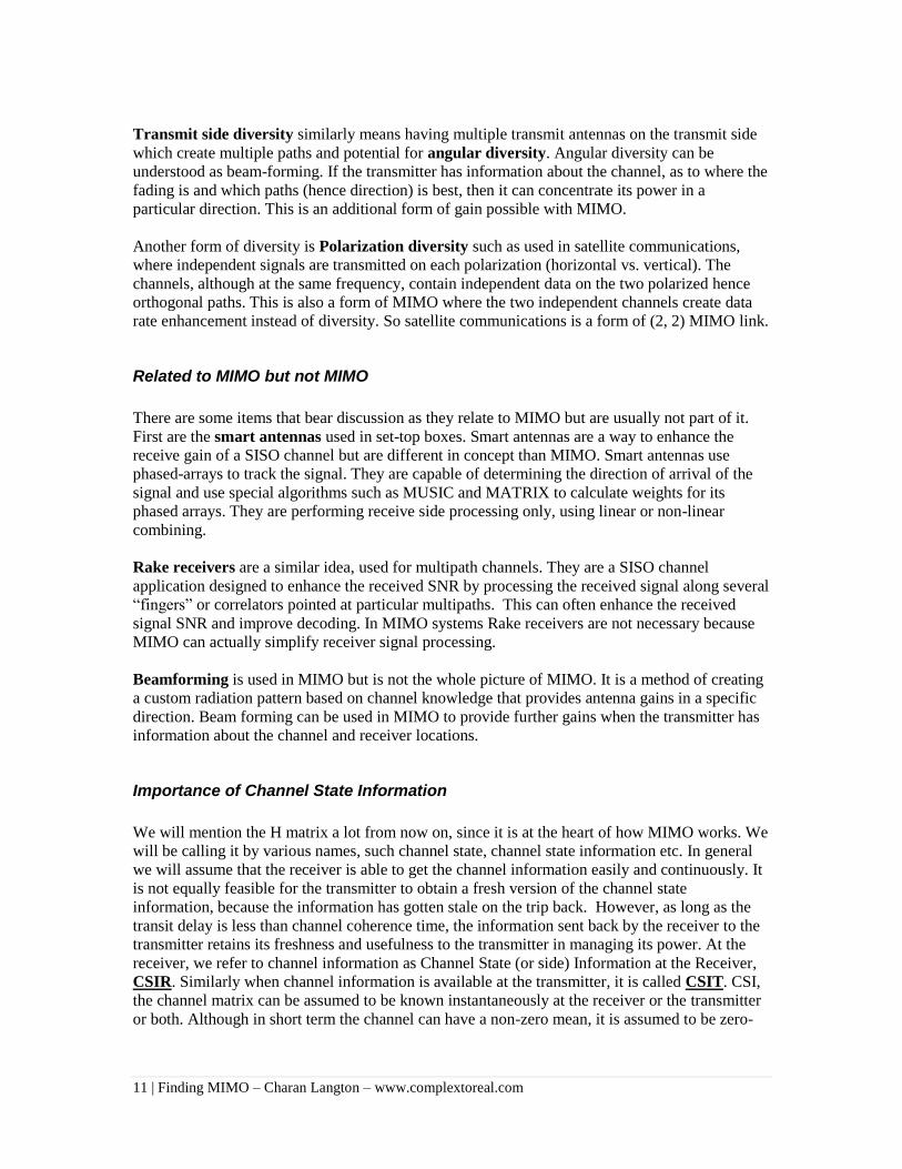
Transmit side diversity similarly means having multiple transmit antennas on the transmit side
which create multiple paths and potential for angular diversity. Angular diversity can be
understood as beam-forming. If the transmitter has information about the channel, as to where the
fading is and which paths (hence direction) is best, then it can concentrate its power in a
particular direction. This is an additional form of gain possible with MIMO.
Another form of diversity is Polarization diversity such as used in satellite communications,
where independent signals are transmitted on each polarization (horizontal vs. vertical). The
channels, although at the same frequency, contain independent data on the two polarized hence
orthogonal paths. This is also a form of MIMO where the two independent channels create data
rate enhancement instead of diversity. So satellite communications is a form of (2, 2) MIMO link.
Related to MIMO but not MIMO
There are some items that bear discussion as they relate to MIMO but are usually not part of it.
First are the smart antennas used in set-top boxes. Smart antennas are a way to enhance the
receive gain of a SISO channel but are different in concept than MIMO. Smart antennas use
phased-arrays to track the signal. They are capable of determining the direction of arrival of the
signal and use special algorithms such as MUSIC and MATRIX to calculate weights for its
phased arrays. They are performing receive side processing only, using linear or non-linear
combining.
Rake receivers are a similar idea, used for multipath channels. They are a SISO channel
application designed to enhance the received SNR by processing the received signal along several
“fingers” or correlators pointed at particular multipaths. This can often enhance the received
signal SNR and improve decoding. In MIMO systems Rake receivers are not necessary because
MIMO can actually simplify receiver signal processing.
Beamforming is used in MIMO but is not the whole picture of MIMO. It is a method of creating
a custom radiation pattern based on channel knowledge that provides antenna gains in a specific
direction. Beam forming can be used in MIMO to provide further gains when the transmitter has
information about the channel and receiver locations.
Importance of Channel State Information
We will mention the H matrix a lot from now on, since it is at the heart of how MIMO works. We
will be calling it by various names, such channel state, channel state information etc. In general
we will assume that the receiver is able to get the channel information easily and continuously. It
is not equally feasible for the transmitter to obtain a fresh version of the channel state
information, because the information has gotten stale on the trip back. However, as long as the
transit delay is less than channel coherence time, the information sent back by the receiver to the
transmitter retains its freshness and usefulness to the transmitter in managing its power. At the
receiver, we refer to channel information as Channel State (or side) Information at the Receiver,
CSIR. Similarly when channel information is available at the transmitter, it is called CSIT. CSI,
the channel matrix can be assumed to be known instantaneously at the receiver or the transmitter
or both. Although in short term the channel can have a non-zero mean, it is assumed to be zero-
12 | Finding MIMO – Charan Langton – www.complextoreal.com
mean and uncorrelated on all paths. When the paths are correlated, then clearly, we have less
information to exploit. But we can still make the channel work.
Channel information can be extracted by monitoring the received gains of a known sequence. In
Time Division Duplex (TDD) communications where both transmitter and the receiver are on the
same frequency, the channel condition is readily available to the transmitter. In Frequency
Division Duplex (FDD) communications, since the forward and reverse links are at different
frequencies, this requires a special feedback link from the receiver to the transmitter. In fact
receive diversity alone is very effective but it places greater burden on the smaller handheld
receivers, requiring larger weight, size and complex signal processing hence increasing cost.
Transmit diversity is easier to implement from a system point of view because the base station
towers in a cell system are not limited by power or weight. In addition to adding more transmit
antennas on the base station towers, space-time coding is also used by the transmitters. This
makes the signal processing required at the receiver simpler.
MIMO Gains
Our goal is to transmit and receive data over several independently fading channels such that the
composite performance mitigates deep fades on any of the channels. To see how MIMO
enhances performance in a fading or multipath channel, we first examine the BER for a BPSK
signal as a function of the receive SNR. [8; 7]
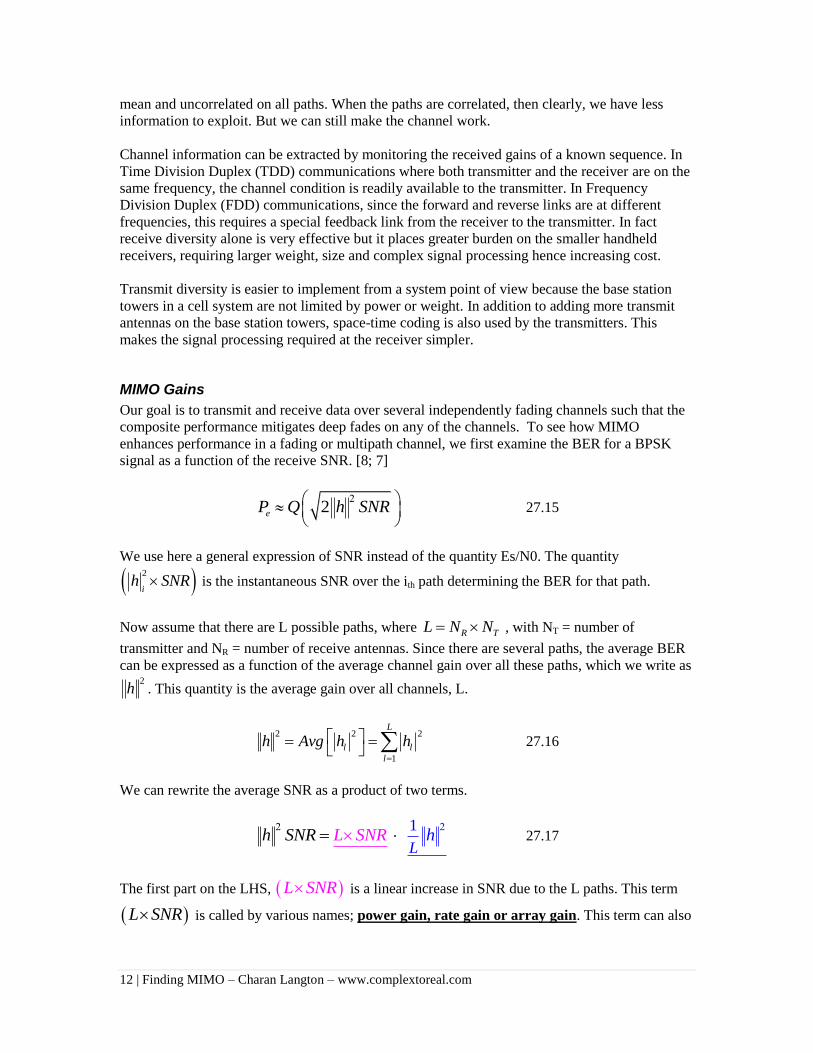
2eP Q h SNR
27.15
We use here a general expression of SNR instead of the quantity Es/N0. The quantity
2
ih SNR is the instantaneous SNR over the ith path determining the BER for that path.
Now assume that there are L possible paths, where R TL N N , with NT = number of
transmitter and NR = number of receive antennas. Since there are several paths, the average BER
can be expressed as a function of the average channel gain over all these paths, which we write as 2
h . This quantity is the average gain over all channels, L.
2 2 2
1
L
l l
l
h Avg h h
27.16
We can rewrite the average SNR as a product of two terms.
1
LL SNR hh SNR
27.17
The first part on the LHS, L SNR is a linear increase in SNR due to the L paths. This term
L SNR is called by various names; power gain, rate gain or array gain. This term can also
13 | Finding MIMO – Charan Langton – www.complextoreal.com
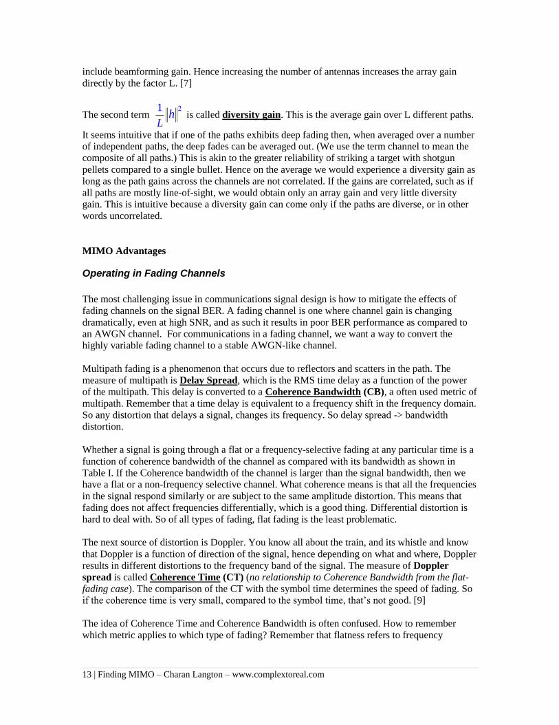
include beamforming gain. Hence increasing the number of antennas increases the array gain
directly by the factor L. [7]
The second term 1
Lh
is called diversity gain. This is the average gain over L different paths.
It seems intuitive that if one of the paths exhibits deep fading then, when averaged over a number
of independent paths, the deep fades can be averaged out. (We use the term channel to mean the
composite of all paths.) This is akin to the greater reliability of striking a target with shotgun
pellets compared to a single bullet. Hence on the average we would experience a diversity gain as
long as the path gains across the channels are not correlated. If the gains are correlated, such as if
all paths are mostly line-of-sight, we would obtain only an array gain and very little diversity
gain. This is intuitive because a diversity gain can come only if the paths are diverse, or in other
words uncorrelated.
MIMO Advantages
Operating in Fading Channels
The most challenging issue in communications signal design is how to mitigate the effects of
fading channels on the signal BER. A fading channel is one where channel gain is changing
dramatically, even at high SNR, and as such it results in poor BER performance as compared to
an AWGN channel. For communications in a fading channel, we want a way to convert the
highly variable fading channel to a stable AWGN-like channel.
Multipath fading is a phenomenon that occurs due to reflectors and scatters in the path. The
measure of multipath is Delay Spread, which is the RMS time delay as a function of the power
of the multipath. This delay is converted to a Coherence Bandwidth (CB), a often used metric of
multipath. Remember that a time delay is equivalent to a frequency shift in the frequency domain.
So any distortion that delays a signal, changes its frequency. So delay spread -> bandwidth
distortion.
Whether a signal is going through a flat or a frequency-selective fading at any particular time is a
function of coherence bandwidth of the channel as compared with its bandwidth as shown in
Table I. If the Coherence bandwidth of the channel is larger than the signal bandwidth, then we
have a flat or a non-frequency selective channel. What coherence means is that all the frequencies
in the signal respond similarly or are subject to the same amplitude distortion. This means that
fading does not affect frequencies differentially, which is a good thing. Differential distortion is
hard to deal with. So of all types of fading, flat fading is the least problematic.
The next source of distortion is Doppler. You know all about the train, and its whistle and know
that Doppler is a function of direction of the signal, hence depending on what and where, Doppler
results in different distortions to the frequency band of the signal. The measure of Doppler
spread is called Coherence Time (CT) (no relationship to Coherence Bandwidth from the flat-
fading case). The comparison of the CT with the symbol time determines the speed of fading. So
if the coherence time is very small, compared to the symbol time, that’s not good. [9]
The idea of Coherence Time and Coherence Bandwidth is often confused. How to remember
which metric applies to which type of fading? Remember that flatness refers to frequency
14 | Finding MIMO – Charan Langton – www.complextoreal.com
response and not to time. So Coherence Bandwidth determines whether a channel is considered
flat or not.
Coherence Time, on the other hand has to do with changes over time, which is related to motion.
Coherence Time is the duration during which a channel appears to be unchanging. So think about
Coherence Time when Doppler or motion is present. When Coherence Time is longer than
symbol time, then we have a slow fading channel and when symbol time is longer than
Coherence time, then we have a fast fading channel. So slowness and fastness mean time based
fading.
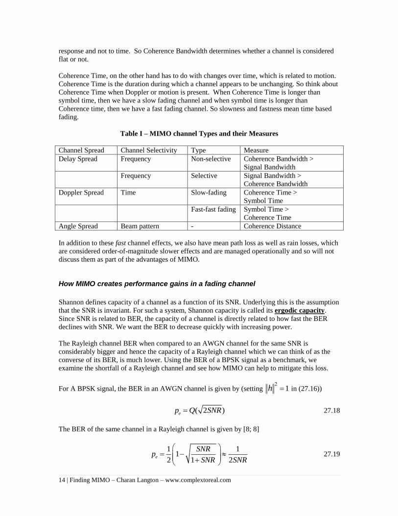
Table I – MIMO channel Types and their Measures
Channel Spread Channel Selectivity Type Measure
Delay Spread Frequency Non-selective Coherence Bandwidth >
Signal Bandwidth
Frequency Selective Signal Bandwidth >
Coherence Bandwidth
Doppler Spread Time Slow-fading Coherence Time >
Symbol Time
Fast-fast fading Symbol Time >
Coherence Time
Angle Spread Beam pattern - Coherence Distance
In addition to these fast channel effects, we also have mean path loss as well as rain losses, which
are considered order-of-magnitude slower effects and are managed operationally and so will not
discuss them as part of the advantages of MIMO.
How MIMO creates performance gains in a fading channel
Shannon defines capacity of a channel as a function of its SNR. Underlying this is the assumption
that the SNR is invariant. For such a system, Shannon capacity is called its ergodic capacity.
Since SNR is related to BER, the capacity of a channel is directly related to how fast the BER
declines with SNR. We want the BER to decrease quickly with increasing power.
The Rayleigh channel BER when compared to an AWGN channel for the same SNR is
considerably bigger and hence the capacity of a Rayleigh channel which we can think of as the
converse of its BER, is much lower. Using the BER of a BPSK signal as a benchmark, we
examine the shortfall of a Rayleigh channel and see how MIMO can help to mitigate this loss.
For A BPSK signal, the BER in an AWGN channel is given by (setting 1h in (27.16))
( 2 )ep Q SNR 27.18
The BER of the same channel in a Rayleigh channel is given by [8; 8]
1 1
12 1 2
e
SNRp
SNR SNR
27.19
15 | Finding MIMO – Charan Langton – www.complextoreal.com
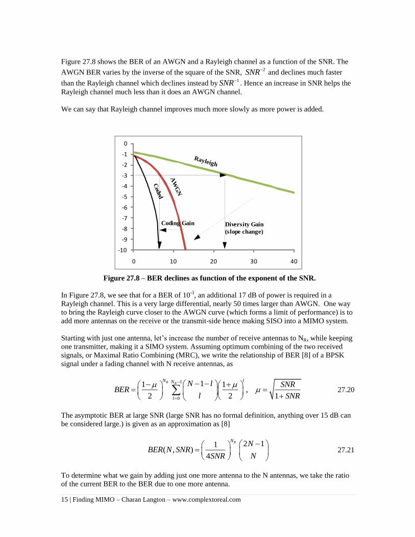
Figure 27.8 shows the BER of an AWGN and a Rayleigh channel as a function of the SNR. The
AWGN BER varies by the inverse of the square of the SNR, 2SNR and declines much faster
than the Rayleigh channel which declines instead by1SNR. Hence an increase in SNR helps the
Rayleigh channel much less than it does an AWGN channel.
We can say that Rayleigh channel improves much more slowly as more power is added.
-10
-9
-8
-7
-6
-5
-4
-3
-2
-1
0
0 10 20 30 40
Diversity Gain
(slope change)
Coding Gain
Rayleigh
AW
GN
Cod
ed
Figure 27.8 – BER declines as function of the exponent of the SNR.
In Figure 27.8, we see that for a BER of 10-3
, an additional 17 dB of power is required in a
Rayleigh channel. This is a very large differential, nearly 50 times larger than AWGN. One way
to bring the Rayleigh curve closer to the AWGN curve (which forms a limit of performance) is to
add more antennas on the receive or the transmit-side hence making SISO into a MIMO system.
Starting with just one antenna, let’s increase the number of receive antennas to NR, while keeping
one transmitter, making it a SIMO system. Assuming optimum combining of the two received
signals, or Maximal Ratio Combining (MRC), we write the relationship of BER [8] of a BPSK
signal under a fading channel with N receive antennas, as
1
0
11 1,
2 2 1
R RN lN
l
N l SNRBER
l SNR
27.20
The asymptotic BER at large SNR (large SNR has no formal definition, anything over 15 dB can
be considered large.) is given as an approximation as [8]
2 11
( , )4
RNN
BER N SNRNSNR
27.21
To determine what we gain by adding just one more antenna to the N antennas, we take the ratio
of the current BER to the BER due to one more antenna.
16 | Finding MIMO – Charan Langton – www.complextoreal.com
( , ) 1
1( 1, ) 2 1
BER N SNRSNR
BER N SNR N
27.22
The gain from adding one more antenna is equal to SNR multiplied by a delta increase in SNR.
The delta increase diminishes as more and more antennas are added. The largest gain is seen
when going from a single antenna to two antennas, (1.5 for going from 1 to 2 vs. 1.1 for going
from 4 to 5 antennas). This delta increase is similar in magnitude to the slope of the BER curve at
large SNR.
Formally, a parameter called Diversity order d, is defined as the slope of the BER curve as a
function of SNR in the region of high SNR.
( )
lim logSNR
BER SNRd
SNR 27.23
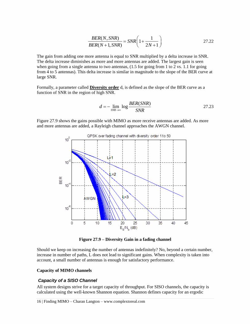
Figure 27.9 shows the gains possible with MIMO as more receive antennas are added. As more
and more antennas are added, a Rayleigh channel approaches the AWGN channel.
Figure 27.9 – Diversity Gain in a fading channel
Should we keep on increasing the number of antennas indefinitely? No, beyond a certain number,
increase in number of paths, L does not lead to significant gains. When complexity is taken into
account, a small number of antennas is enough for satisfactory performance.
Capacity of MIMO channels
Capacity of a SISO Channel
All system designs strive for a target capacity of throughput. For SISO channels, the capacity is
calculated using the well-known Shannon equation. Shannon defines capacity for an ergodic
17 | Finding MIMO – Charan Langton – www.complextoreal.com
channel that data rate which can be transmitted with asymptotically small probability of error.
The capacity of such a channel is given in terms of bits/sec or by normalizing with bandwidth by
bits/sec/Hz. The second formulation (27.26) allows easier comparison and is the one used more
often. It is also bandwidth independent.
2
0
log (1 ) /P
C W b sN W
27.24
2log (1 ) / /SNR b s Hz 27.25
At high SNRs, ignoring the addition of 1 to SNR, the capacity is a direct function of SNR.
2log ( )C SNR 27.26
This capacity is based on a constant data rate and is not a function of whether channel state
information is available to the receiver or the transmitter. This result is applicable only to ergodic
channels, ones where the data rate is fixed and SNR is stable.
Capacity of MIMO Channels
We know from Shanon’s equation that a particular SNR can give only a fixed maximum capacity.
If SNR goes down, so will the ability of the channel to pass data. In a fading channel, the SNR is
constantly changing. As the rate of fade changes, the capacity changes with it.
We can use a fixed H matrix as our benchmark of performance where the basic assumption is
that, for that one realization, the channel is fixed and hence has an ergodic channel capacity. In
other words, for just that little time period, the channel is behaving like an AWGN channel. We
then break a channel into portions of either time or frequency so that in small segments, even in a
frequency-selective channel with Doppler, channel can be treated as having a fixed realization of
the H matrix, i.e. allowing us to think of it instantaneously as a AWGN channel. We can perform
the capacity calculations over several realizations of H matrix and then compute average capacity
over these. In flat fading channels the channel matrix may remain constant and or may change
very slowly. However, with user motion, this assumption does not hold.
Before delving into capacity calculations, we will look at how a MIMO matrix channel can be
decomposed into parallel independent channels. This method provides an alternate way to look at
the capacity of a MIMO system.
Decomposing a MIMO channel into parallel independent channels
Conceptually we think of MIMO as transmission of same data over multiple antennas, hence it is
a matrix channel. But there is a mathematical trick that lets us decompose the MIMO channel into
several independent parallel channels each of which can be thought of as a SISO channel. To look
at a MIMO channel as a set of independent channels, we use an algorithm that comes from linear
algebra, the Singular Value Decomposition (SVD). The process requires pre-coding at the
transmitter and receiver shaping at the receiver. It may look hard to understand but it is just
matrix math.
18 | Finding MIMO – Charan Langton – www.complextoreal.com
Input and output auto-correlation
Assume that a MIMO channel has N transmitters and M receivers. The transmitted vector across
NT antennas is given by 1 2, ,TNx x x . We assume that individual transmit signals consist of
symbols that are zero mean circular-symmetric complex Gaussian variables. (A vector x is said to
be circular-symmetric if je
x has same distribution for all . ) The covariance matrix for the
transmitted symbols is written as
H
xx ER xx 27.27
Where symbol H stands for the transpose and component-wise complex conjugate of the matrix
(also called Hermitian) and not the channel matrix. This relationship gives us a measure of
correlated-ness of the transmitted signal amplitudes.
When the powers of the transmitted symbols are the same, what we get is a scaled identity matrix.
For a (3×3) MIMO system of total power of PT, equally distributed we would write this matrix as
1 0 0
0 1 0
0 0 1
xx TP
R
If the same system distributes the power differently say in ratio of 1: 2: 3, then the covariance
matrix would be
1 0 0
0 2 0
0 0 3
xx TP
R
If we assume that the total transmitted power is PT and is equal to trace of the Input covariance
matrix, we can write the total power of the transmitted signal as the trace of the covariance
matrix.
xxP tr R 27.28
The received signal is given by
n r Hx 27.29
The noise matrix (N×1) components are assumed to be ZMGV (zero-mean Gaussian variable) of
equal variance. We can write the covariance matrix of the noise process similar to the transmit
symbols as
HEnnR nn 27.30
And since there is no correlation between its rows, we can write this as
19 | Finding MIMO – Charan Langton – www.complextoreal.com
2
nn MR I 27.31
Which says that each of the M received noise signals is an independent signal of noise variance, 2 . Each receiver receives a complex signal consisting of the sum of the replicas from N
transmit antennas and an independent noise signal.
If we assume that the power received at each receiver is not the same, we write the SNR of the
mth receiver as
2
mm
P
27.32
where Pm is some part of the total power. However the average SNR for all receive antennas
would still be equal to 2
TP
, where PT is total power because
1
TN
T m
m
P P
Now we write the covariance matrix of the receive signal using eq. (27.33) as
H rr xx nnR HR H R 27.33
where Rxx is the covariance matrix of the transmitted signal. The total receive power is equal to
the trace of the matrix Rrr.
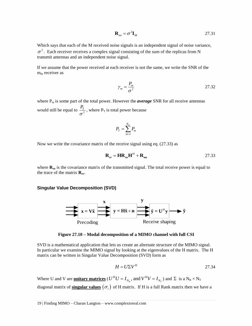
Singular Value Decomposition (SVD)
Figure 27.10 – Modal decomposition of a MIMO channel with full CSI
SVD is a mathematical application that lets us create an alternate structure of the MIMO signal.
In particular we examine the MIMO signal by looking at the eigenvalues of the H matrix. The H
matrix can be written in Singular Value Decomposition (SVD) form as
HH U V 27.34
Where U and V are unitary matrices ( , andR T
H H
N NU U I V V I ) and is a NR × NT
diagonal matrix of singular values i of H matrix. If H is a full Rank matrix then we have a
x
yx = VxH
y = U yy = Hx n
y
Precoding Receive shaping
20 | Finding MIMO – Charan Langton – www.complextoreal.com
min( , )R TN N of non-zero singular values, hence the same number of independent channels. The
parallel decomposition is essentially a linear mapping function performed by pre-coding the input
signal x , consisting of multiplying it with matrix V, such that x V x .
The received signal y is given by multiplying it with H
U ,
( )Hy U Hx +n 27.35
Now multiplying it out, and setting value of H from (27.35), we get
( )H Hy U UΣV x+n
Now substitute
x V x into above. We get
( )
( )
H H
H H
H H H
V
y U UΣV x+n
U UΣV x+n
U UΣV Vx+U n
x n
27.36
In the last result we see that the output signal is in form of a pre-coded input signal x times the
singular value matrix, . Note that the multiplication of noise n, by the unitary matrix UH does
not change the noise distribution. [10]
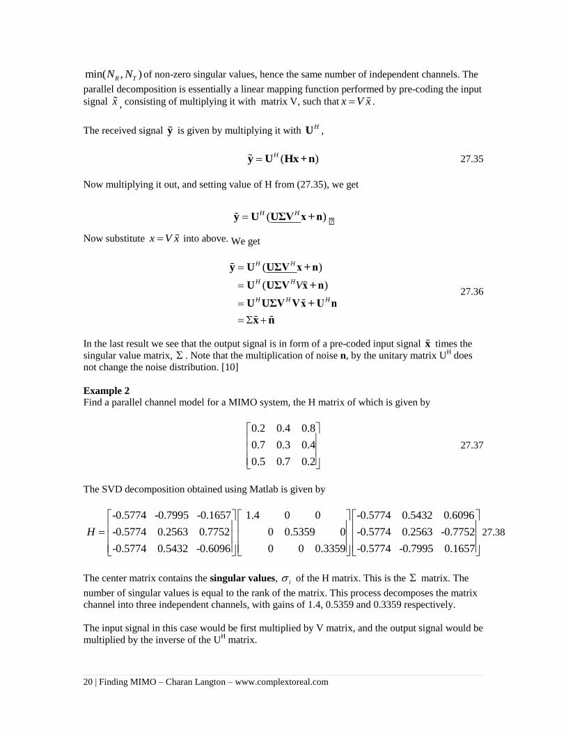
Example 2
Find a parallel channel model for a MIMO system, the H matrix of which is given by
0.2 0.4 0.8
0.7 0.3 0.4
0.5 0.7 0.2
27.37
The SVD decomposition obtained using Matlab is given by
-0.5774 -0.7995 -0.1657 1.4 0 0 -0.5774 0.
-0.5774 0.2563 0.7752 0 0.5359 0
-0.5774 0.5432 -0.6096 0 0 0.3359
H
5432 0.6096
-0.5774 0.2563 -0.7752
-0.5774 -0.7995 0.1657
27.38
The center matrix contains the singular values, i of the H matrix. This is the matrix. The
number of singular values is equal to the rank of the matrix. This process decomposes the matrix
channel into three independent channels, with gains of 1.4, 0.5359 and 0.3359 respectively.
The input signal in this case would be first multiplied by V matrix, and the output signal would be
multiplied by the inverse of the UH matrix.
21 | Finding MIMO – Charan Langton – www.complextoreal.com
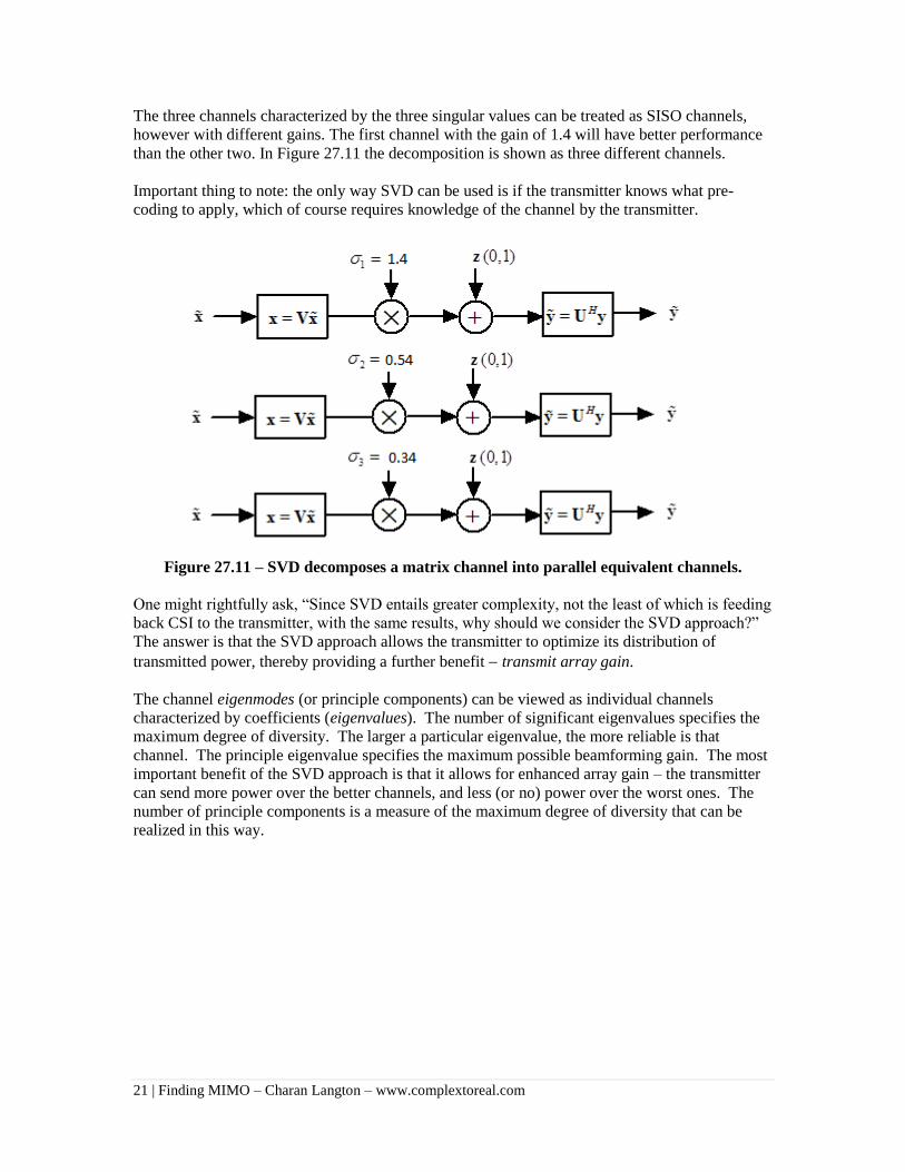
The three channels characterized by the three singular values can be treated as SISO channels,
however with different gains. The first channel with the gain of 1.4 will have better performance
than the other two. In Figure 27.11 the decomposition is shown as three different channels.
Important thing to note: the only way SVD can be used is if the transmitter knows what pre-
coding to apply, which of course requires knowledge of the channel by the transmitter.
Figure 27.11 – SVD decomposes a matrix channel into parallel equivalent channels.
One might rightfully ask, “Since SVD entails greater complexity, not the least of which is feeding
back CSI to the transmitter, with the same results, why should we consider the SVD approach?”
The answer is that the SVD approach allows the transmitter to optimize its distribution of
transmitted power, thereby providing a further benefit transmit array gain.
The channel eigenmodes (or principle components) can be viewed as individual channels
characterized by coefficients (eigenvalues). The number of significant eigenvalues specifies the
maximum degree of diversity. The larger a particular eigenvalue, the more reliable is that
channel. The principle eigenvalue specifies the maximum possible beamforming gain. The most
important benefit of the SVD approach is that it allows for enhanced array gain – the transmitter
can send more power over the better channels, and less (or no) power over the worst ones. The
number of principle components is a measure of the maximum degree of diversity that can be
realized in this way.
22 | Finding MIMO – Charan Langton – www.complextoreal.com
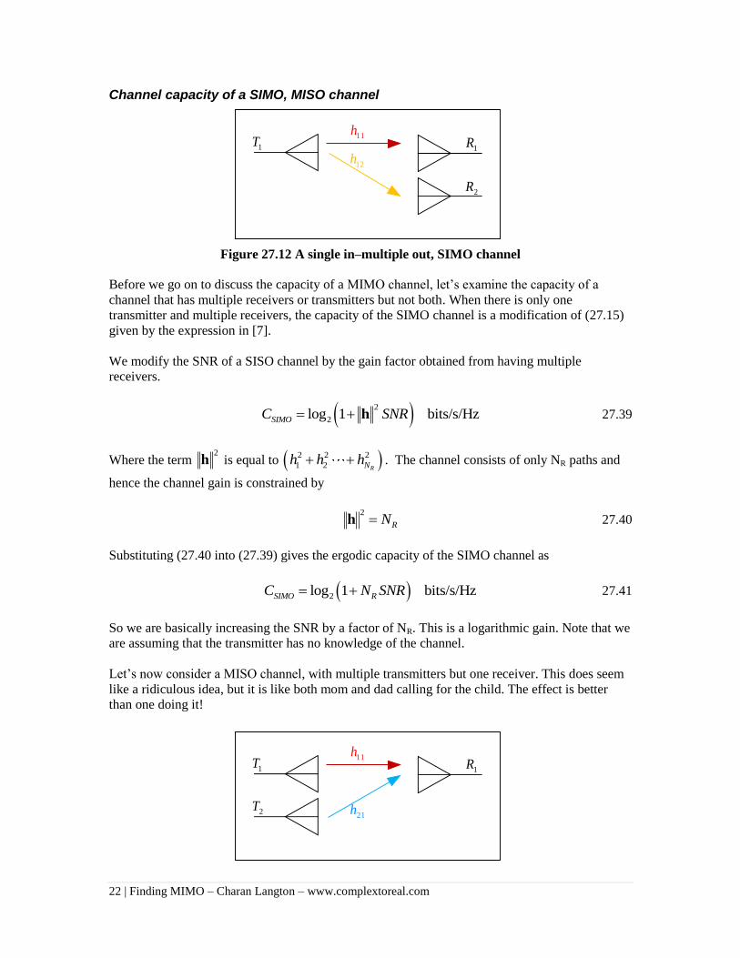
Channel capacity of a SIMO, MISO channel
11h
12h1T
2R
1R
Figure 27.12 A single in–multiple out, SIMO channel
Before we go on to discuss the capacity of a MIMO channel, let’s examine the capacity of a
channel that has multiple receivers or transmitters but not both. When there is only one
transmitter and multiple receivers, the capacity of the SIMO channel is a modification of (27.15)
given by the expression in [7].
We modify the SNR of a SISO channel by the gain factor obtained from having multiple
receivers.
2
2log 1 bits/s/HzSIMOC SNR h 27.39
Where the term 2
h is equal to 2 2 2
1 2 RNh h h . The channel consists of only NR paths and
hence the channel gain is constrained by
2
RNh 27.40
Substituting (27.40 into (27.39) gives the ergodic capacity of the SIMO channel as
2log 1 bits/s/HzSIMO RC N SNR 27.41
So we are basically increasing the SNR by a factor of NR. This is a logarithmic gain. Note that we
are assuming that the transmitter has no knowledge of the channel.
Let’s now consider a MISO channel, with multiple transmitters but one receiver. This does seem
like a ridiculous idea, but it is like both mom and dad calling for the child. The effect is better
than one doing it!
11h
21h2T
1T1R
23 | Finding MIMO – Charan Langton – www.complextoreal.com
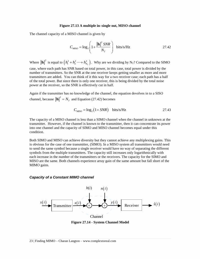
Figure 27.13 A multiple in–single out, MISO channel
The channel capacity of a MISO channel is given by
2
2log 1 bits/s/HzMISO
T
SNRC
N
h 27.42
Where 2
h is equal to 2 2 2
1 2 TNh h h . Why are we dividing by NT? Compared to the SIMO
case, where each path has SNR based on total power, in this case, total power is divided by the
number of transmitters. So the SNR at the one receiver keeps getting smaller as more and more
transmitters are added. You can think of it this way for a two receiver case; each path has a half
of the total power. But since there is only one receiver, this is being divided by the total noise
power at the receiver, so the SNR is effectively cut in half.
Again if the transmitter has no knowledge of the channel, the equation devolves in to a SISO
channel, because 2
TNh and Equation (27.42) becomes
2log 1 bits/s/HzMISOC SNR 27.43
The capacity of a MISO channel is less than a SIMO channel when the channel in unknown at the
transmitter. However, if the channel is known to the transmitter, then it can concentrate its power
into one channel and the capacity of SIMO and MISO channel becomes equal under this
condition.
Both SIMO and MISO can achieve diversity but they cannot achieve any multiplexing gains. This
is obvious for the case of one transmitter, (SIMO). In a MISO system all transmitters would need
to send the same symbol because a single receiver would have no way of separating the different
symbols from the multiple transmitters. The capacity still increases only logarithmically with
each increase in the number of the transmitters or the receivers. The capacity for the SIMO and
MISO are the same. Both channels experience array gain of the same amount but fall short of the
MIMO gains.
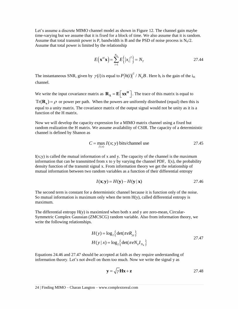
Capacity of a Constant MIMO channel
Transmitter x i
Receiver
( )h i
s i
n i
y i s i
Channel
Figure 27.14 - System Channel Model
24 | Finding MIMO – Charan Langton – www.complextoreal.com
Let’s assume a discrete MIMO channel model as shown in Figure 12. The channel gain maybe
time-varying but we assume that it is fixed for a block of time. We also assume that it is random.
Assume that total transmit power is P, bandwidth is B and the PSD of noise process is N0/2.
Assume that total power is limited by the relationship
2
1
TNH
i T
i
E E x N
x x 27.44
The instantaneous SNR, given by ( )i is equal to2
0( ) /P h i N B . Here hi is the gain of the ith
channel.
We write the input covariance matrix as H
XR E xx . The trace of this matrix is equal to
Tr( ) xR or power per path. When the powers are uniformly distributed (equal) then this is
equal to a unity matrix. The covariance matrix of the output signal would not be unity as it is a
function of the H matrix.
Now we will develop the capacity expression for a MIMO matrix channel using a fixed but
random realization the H matrix. We assume availability of CSIR. The capacity of a deterministic
channel is defined by Shanon as
( )
max ( ; ) bits/channel usef x
C I x y 27.45
I(x;y) is called the mutual information of x and y. The capacity of the channel is the maximum
information that can be transmitted from x to y by varying the channel PDF, f(x), the probability
density function of the transmit signal x. From information theory we get the relationship of
mutual information between two random variables as a function of their differential entropy
( ; ) ( ) ( | )I H H x y y y x 27.46
The second term is constant for a deterministic channel because it is function only of the noise.
So mutual information is maximum only when the term H(y), called differential entropy is
maximum.
The differential entropy H(y) is maximized when both x and y are zero-mean, Circular-
Symmetric Complex Gaussian (ZMCSCG) random variable. Also from information theory, we
write the following relationships.
2
2 0
( ) log det(
( | ) log det(R
yy
N
H y eR
H y x eN I
27.47
Equations 24.46 and 27.47 should be accepted at faith as they require understanding of
information theory. Let’s not dwell on them too much. Now we write the signal y as
y Hx z 27.48
25 | Finding MIMO – Charan Langton – www.complextoreal.com
Here is instantaneous SNR. The auto-correlation of the output signal y which we need for
(27.48) is given by
0 R
H
yy
H H H
H H H
H H H
H
xx N
R E
E
E
E E
HR H N I
yy
Hx z x H z
Hxx H zz
H xx H zz
27.49
From here we can write the expression for capacity as
2( )
( ; ) max log detR
xx T
H
N xxTr R N
T
SNRC I x y I HR H
N
27.50
When CSIT is not available, we can assume equal power distribution among the transmitters, in
which case Rxx is an identity matrix and the equation becomes
2log detR
H
N
T
SNRC I
N
HH 27.51
This is the capacity equation for MIMO channels with equal power. (Figure 27.3) The
optimization of this expression depends on whether or not the CSI (H matrix) is known to the
transmitter.
Now note that as the number of antennas increases, we get
1
lim H
NN M
HH I 27.52
Intuitively this means that as the number of paths goes to infinity, the power that reaches each of
the infinite number of receivers becomes equal and the channel now approaches an AWGN
channel.
This gives us an expression about the capacity limit of a NT × NR MIMO system by substituting
(27.52) into (27.51),
2log detRNC M I SNR
where M is the minimum of NT and NR, the number of the antennas. So now finally we see how
the capacity increases linearly with M, the minimum of (NT, NR). This is an important finding. If
a system has (4, 6) antennas, then the maximum diversity that can be obtained is of order 4, the
small number of the two system parameters.
26 | Finding MIMO – Charan Langton – www.complextoreal.com
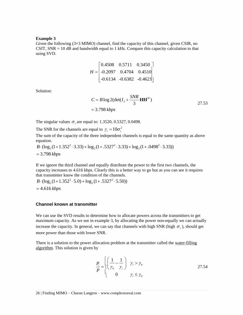
Example 3
Given the following (3×3 MIMO) channel, find the capacity of this channel, given CSIR, no
CSIT, SNR = 10 dB and bandwidth equal to 1 kHz. Compare this capacity calculation to that
using SVD.
0.4508 0.5711 0.3450
-0.2097 0.4704 0.4510
-0.6134 -0.6382 -0.4621
H
Solution:
3log 2(det( )
3
3.798
HSNRC B I
kbps
HH 27.53
The singular values i are equal to: 1.3520, 0.5327, 0.0498.
The SNR for the channels are equal to 210i i
The sum of the capacity of the three independent channels is equal to the same quantity as above
equation. 2 2 2
2 2 2(log (1 1.352 3.33) log (1 .5327 3.33) log (1 .0498 3.33))
3.798
B
kbps
If we ignore the third channel and equally distribute the power to the first two channels, the
capacity increases to 4.616 kbps. Clearly this is a better way to go but as you can see it requires
that transmitter know the condition of the channels. 2 2
2 2(log (1 1.352 5.0) log (1 .5327 5.50))
4.616
B
kbps
Channel known at transmitter
We can use the SVD results to determine how to allocate powers across the transmitters to get
maximum capacity. As we see in example 3, by allocating the power non-equally we can actually
increase the capacity. In general, we can say that channels with high SNR (high i ), should get
more power than those with lower SNR.
There is a solution to the power allocation problem at the transmitter called the water-filling
algorithm. This solution is given by
0
0
0
1 1
0
iii
i
P
P
27.54
27 | Finding MIMO – Charan Langton – www.complextoreal.com
Where 0 is a threshold constant. Here i is the SNR of the ith channel.
We are comparing the inverse of the threshold with the inverse of the channel SNR. If the
inverse difference is less than the threshold, we do not allocate any power to the ith channel. If the
difference is positive then we say, “Hay this channel has life, let’s give it some more power to see
if it helps the overall performance.”
The capacity using the water-filling algorithm is given by
0
2
: 0
logi
i
i
C B
27.55
The thing about water-filling algorithm is that it is much easier to comprehend then is it to
describe using equations. Think of it as a boat sinking in the water. Where would you sit on the
boat while waiting for rescue, clearly the part that is sticking above the water, right? The
analogous part above the surface are the channels that can overcome fading. Some of the channels
reach the receiver with enough SNR for decoding. So our data/power should go to these channels
and not to the ones that are under water. So basically, we allocate power to those channels that are
strongest or above a pre-set threshold. To weak does not go the spoils!
Example 4
Find the optimum power allocation for the MIMO system of Example 3 assuming total power is 1
W, noise power is equal to 0.1 W and the signal bandwidth is 50 kHz.
The singular values computed for the three channels in Example 2 are 1 1.4, 2 .5359 and
3 .3359. The SNR values for each channel assuming equal power allocation are
1 = 2
(1/ .1) 1.4 19.6
2 = 2
(1/ .1) .5359 2.87
3 = ( 2
(1/ .1) .3359 1.128
We compute the threshold level from (27.54) to get
3
1 0
0
0
1 11
31 ((1/19.6) (1/ 2.87) (1/1.128))
1.3126
i i
Since the third channel with its SNR of 1.128 is less than this threshold value of SNR, we do not
allocate any power to the third channel and redo the calculations based only on the first two
channels. Repeating the calculations for the two channels with higher singular values, we get a
new threshold value of 0 = 1.4294. Both channels are above this level, so we should allocate
proportional power to each. The power allocated to each channel according to the water-filling
algorithm is
28 | Finding MIMO – Charan Langton – www.complextoreal.com
1
2
3
1 1
1.26
1(.793 (1/ 9.73)) 0.691
1(.793 (1/1.875)) 0.261
1(.793 (1/1.343)) 0.0491
i
i
P
P
P W
P W
P W
The total capacity is now equal to
3
2
9.75 1.875 1.34350 10 log 180 bits/sec
1.26C k
The allocation has changed from 0.33 W for each transmitter to almost twice that for the first
transmitter since it has the best gain. The capacity has increased from 41.4 kbps to nearly five
times that.
Channel Capacity in Outage
The Rayleigh channels go through such extremes of SNR fades that the average SNR cannot be
maintained from one time block to the next. Due to this, they are unable to support a constant data
rate. A Rayleigh channel can be characterized as a binary state channel; an ergodic channel but
with an outage probability. When it has a SNR that is above a minimum threshold, it can be
treated as ON and capacity can be calculated using the information-theoretic rate. But when the
SNR is below the threshold, the capacity of the channel is zero. The channel is said to be in
outage.
Although ergodic capacity can be useful in characterizing a fast-fading channel, it is not very
useful for slow-fading, where there can be outages for significant time intervals. When there is
an outage, the channel is so poor that there is no scheme able to communicate reliably at a certain
fixed data rate.
The outage capacity is the capacity that is guaranteed with a certain level of reliability. We
define outage capacity as the information rate that is guaranteed for (100 – p)% of the channel
realizations. A 1% outage probability means that 99% of the time the channel is above a threshold
of SNR and can transmit data. For real systems, outage capacity is the most useful measure of
throughput capability.
Question: which would have higher capacity, a system with 1% outage or 10% outage?
The high probability of outage means, we can set the threshold lower, which also means that
system will have higher capacity, of course only while it is working which is 90% of the time.
We can write the capacity equation of a Rayleigh channel with outage probability , as
2 min(1 ) log (1 )out outC P B 27.56
Where
29 | Finding MIMO – Charan Langton – www.complextoreal.com
min( )outP p 27.57
We can calculate the probability of obtaining a minimum threshold value of the SNR, assuming it
has a Rayleigh distribution.
min
min
/
min
min0
1( )
1
x
out
P e dx
P e
27.58
The capacity of channel under outage probability is given by
2
1ln
1log 1C SNR
27.59
Note that here we have modified the Shanon’s equation by the outage probability, the factor in
blue.
Example 5
If the average received power of a Rayleigh channel is 20 dBm, then what is the probability that
the received power at any time will be less than 2 dBm?
Solution: 20P dbm = 100 mW. The probability that the received power is less than 2 dBm is
equal to
min
1.584
1001 1 0.015 15%outP e e
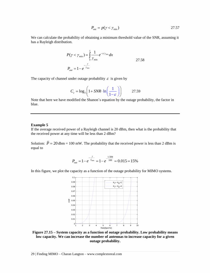
In this figure, we plot the capacity as a function of the outage probability for MIMO systems.
Figure 27.15 – System capacity as a function of outage probability. Low probability means
low capacity. We can increase the number of antennas to increase capacity for a given
outage probability.
1 2 3 4 5 6 7 8 9 100
0.01
0.02
0.03
0.04
0.05
0.06
0.07
0.08
0.09
0.1
Rate[bps/Hz]
CD
F
NT= N
R=2
NT= N
R=4
30 | Finding MIMO – Charan Langton – www.complextoreal.com
Example 6
Assume a fading channel which can take on three different values of channel coefficients ( )h i :
0.4 with probability 0.2, 0.1 with probability 0.5, and 0.2 with probability 0.3. If the transmit
power is 10mW, the noise density N0 = 10-9
W/Hz and the bandwidth of the signal is equal to 50
kHz, find capacity of this fading channel and the capacity of an equivalent AWGN channel of the
same average SNR.
Solution:
The three SNR values are equal to 2
0/iPh N W .
2 9
2 9
2 9
.01 (.4) / (50000 10 ) 32
.01 (.1) / (50000 10 ) 2
.01 (.2) / (50000 10 ) 8
The capacity can be calculated as the sum of three ergodic capacities, one for each SNR.
2
3
2 2 2
log (1 ) ( )
50 10 .2log (1 32) .5log (1 2) .3log (1 8)
41.4
i iC B SNR p SNR
kbps
27.60
Note here, we calculated a separate capacity for each SNR. We assume no average SNR for the
channel.
The equivalent average SNR for an AWGN channel is equal to 0 .2 32 .5 2 .4 8 9.8
The ergodic capacity assuming constant rate for this channel is equal to 3
250 10 log (1 9.8) 51.7 kbps
Compare 51.5 kbps to 41.4 kbps for the fading channel.
Example 7
Find the outage probability of a BPSK signal in a Rayleigh channel with number of antennas
equal to 1, 2 and 4. The average SNR per path is equal to 10 dB and the threshold SNR is 7 dB
0 / 10^.7/10^21 1iM M
outP e e
For M =1, we get, Pout = .1466, M = 2, Pout = .0215 and for M = 4, Pout = 72.13 10 .
This is reflected in the fact that the smaller the outage probability, smaller the number of transmit
antennas that should be used.
Capacity Under a Correlated Channel
We have said a few times already that the MIMO gains come from the independence of the
channels. We assume for the development of ergodic capacity that channels created by MIMO are
independent. But what happens if there is some correlation among the channels which is what
happens in reality due to reflectors located near the base station or the towers. (Usually in cell
31 | Finding MIMO – Charan Langton – www.complextoreal.com
phone systems, the transmitters (on account on being located high on towers) are less subject to
correlation than are the receivers (the cell phones)) We will now examine the effect this has on
the system capacity.
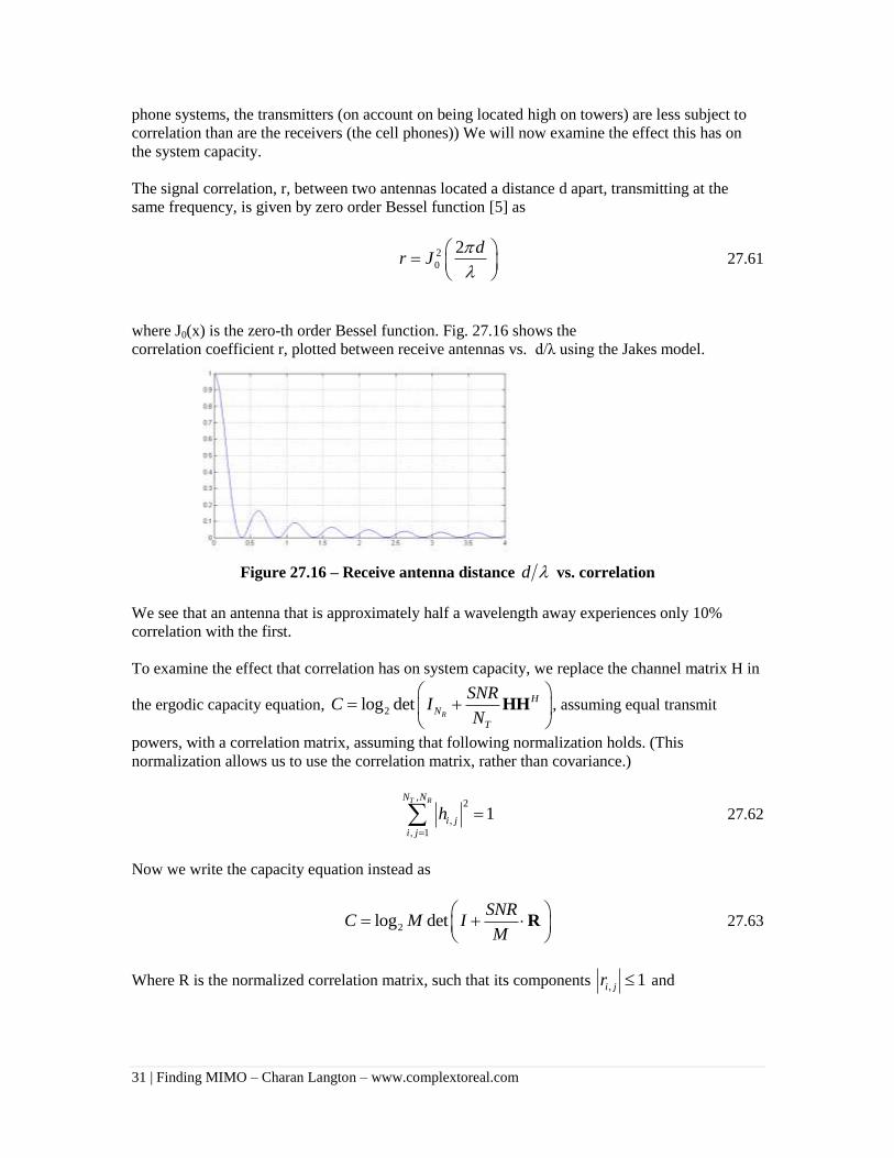
The signal correlation, r, between two antennas located a distance d apart, transmitting at the
same frequency, is given by zero order Bessel function [5] as
2
0
2 dr J
27.61
where J0(x) is the zero-th order Bessel function. Fig. 27.16 shows the
correlation coefficient r, plotted between receive antennas vs. d/λ using the Jakes model.
Figure 27.16 – Receive antenna distance d vs. correlation
We see that an antenna that is approximately half a wavelength away experiences only 10%
correlation with the first.
To examine the effect that correlation has on system capacity, we replace the channel matrix H in
the ergodic capacity equation, 2log detR
H
N
T
SNRC I
N
HH , assuming equal transmit
powers, with a correlation matrix, assuming that following normalization holds. (This
normalization allows us to use the correlation matrix, rather than covariance.)
,2
,
, 1
1T RN N
i j
i j
h
27.62
Now we write the capacity equation instead as
2log detSNR
C M IM
R 27.63
Where R is the normalized correlation matrix, such that its components , 1i jr and
32 | Finding MIMO – Charan Langton – www.complextoreal.com
1
ij ik jk ik jk
k ki j
r h h h h
27.64
We can write the capacity equation as
2 2log det( ) log det( )C M I SNR R
The first underlined part of the expression is the capacity of M independent channels and the
second is the contribution due to correlation. Since the determinant R is always <= 1, then
correlation always results in degradation to the ergodic capacity.
An often used channel model for M = 2, and 4 called the Kronecker Delta model takes this
concept further by separating the correlation into two parts, one near the transmitter and the other
near the receiver, assuming each to be independent of the other. We define two correlation
matrices, one for transmit, RT and one for receiver RR. The complete channel correlation is
assumed to be equal to the Kronecker product of these two smaller matrices.
MIMO R TR R R 27.65
The correlation among the columns of the H matrix represents the correlation between the
transmitter and correlation between rows in receivers. We can write these two one-sided matrices
as
1
1
H
R
TH
T
E
E
R HH
R H H
27.66
The constant parameters (the correlation coefficients for each side) satisfy the relationship
MIMOTr R 27.67
Now if we want to see how correlation at the two ends affects the capacity, we multiply the
random channel H matrix with the two correlation matrices as follows.
How do we get these matrices? In some cases, test data is available which can be used, in others,
we use a generic form based on Bessel coefficients. If we use the correlation coefficient on each
side as a parameter, we can write each correlation matrix as
2 2
2 2
1 1
1 1
1 1
R Tand
R R
Now write the correlated channel matrix in a Cholesky form as
33 | Finding MIMO – Charan Langton – www.complextoreal.com
T w RH R H R 27.68
Where Hw is the i.i.d random H matrix, that is now subject to correlation effects.
The correlation at the transmitter is mathematically seen as correlation between the columns of
the H matrix and we can write it as RT. The correlation at the receiver is seen as the correlation
between the rows of the H matrix, RR. Clearly if the columns are similar, then each antenna is
seeing a similar channel. When the received amplitudes are similar at each receiver then we are
seeing correlation at the receiver.
The H matrix under correlation is ill conditioned, and small changes lead to large changes in the
received signal, clearly not a helpful situation.
The capacity of a channel with correlation can be written as
1/2 1/2
2log detR
H H
N r t
T
SNRC I R H R
N
27.69
When NT = NR and SNR is high, this expression can approximated as
2 2 2log det log det log detR
H
N u u r t
T
SNRC I H H R R
N
27.70
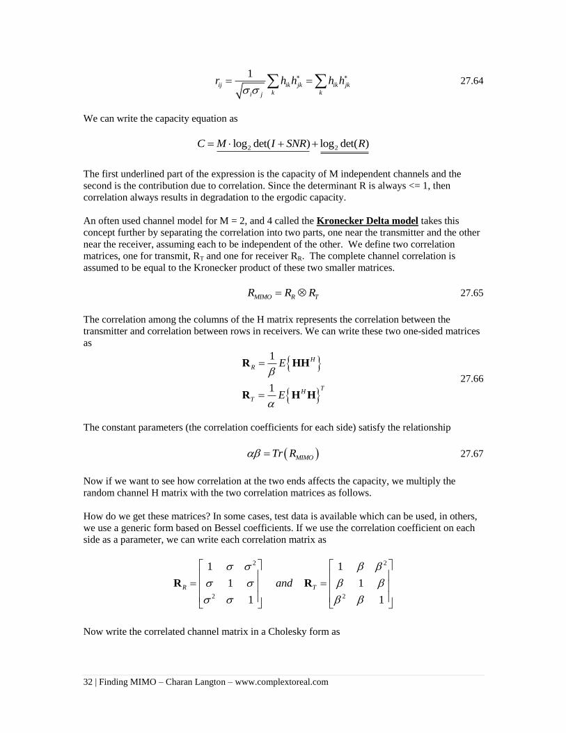
The last two terms are always negative since det( ) 0R . That implies that correlation leads to
reduction in capacity as shown in the case of a 4×4 system with 20% and 40% correlation.
Figure 27.17 – How correlation reduces capacity
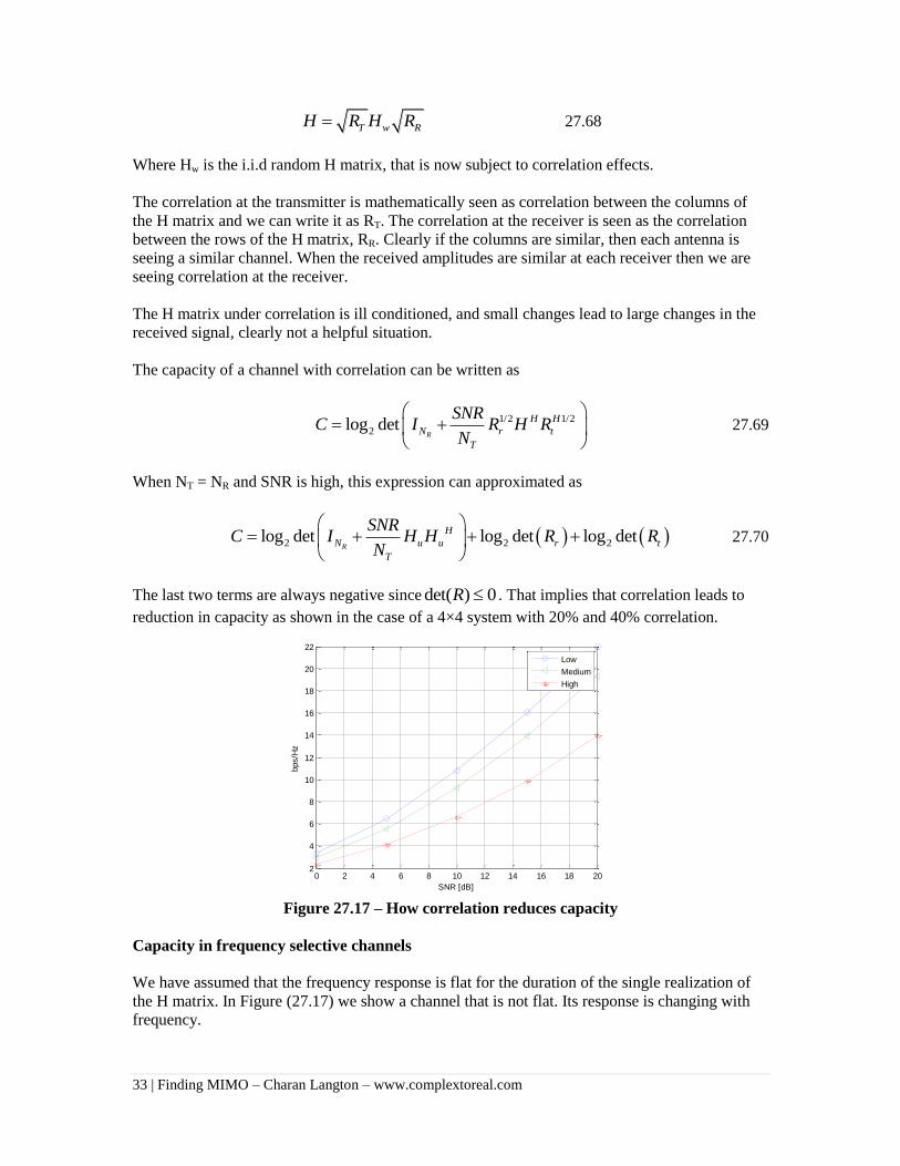
Capacity in frequency selective channels
We have assumed that the frequency response is flat for the duration of the single realization of
the H matrix. In Figure (27.17) we show a channel that is not flat. Its response is changing with
frequency.
0 2 4 6 8 10 12 14 16 18 202
4
6
8
10
12
14
16
18
20
22
SNR [dB]
bps/H
z
Low
Medium
High
34 | Finding MIMO – Charan Langton – www.complextoreal.com
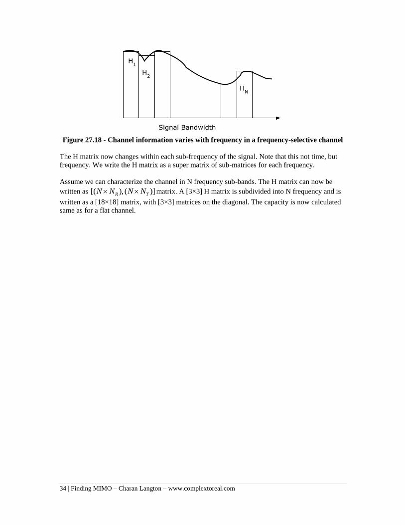
Figure 27.18 - Channel information varies with frequency in a frequency-selective channel
The H matrix now changes within each sub-frequency of the signal. Note that this not time, but
frequency. We write the H matrix as a super matrix of sub-matrices for each frequency.
Assume we can characterize the channel in N frequency sub-bands. The H matrix can now be
written as [( ), ( )]R TN N N N matrix. A [3×3] H matrix is subdivided into N frequency and is
written as a [18×18] matrix, with [3×3] matrices on the diagonal. The capacity is now calculated
same as for a flat channel.
35 | Finding MIMO – Charan Langton – www.complextoreal.com
Spatial multiplexing and how it works
We have been assuming that the each of the links in a MIMO system transmit the same
information. This is an implicit assumption of obtaining diversity gain. Multicasting provides
diversity gain but no data rate improvement. If we could send independent information across the
antennas, then there is an opportunity to increase the data rate as well as keep some diversity
gain. The data rate improvement in a MIMO system is called Spatial Multiplexing Gain (SMG).
The data rate improvement is related to the number of pairs of the RCV/XMT antennas, and when
these numbers are unequal, it is proportional to smaller of the two numbers, NT, NR. This easy to
see; we can only transmit only as many different symbols as there are transmit antennas. This
number is then limited by the number of receive antennas, if the number of receive antennas is
less than the number of transmit antennas.
Spatial multiplexing means the ability to transmit higher bit rate when compared to a system
where we only get diversity gains because we transmit the same symbol from each transmitter.
Just as diversity is defined formally by Equation 27.23, we define spatial multiplexing gain as
limlog( )SNR
rs
SNR 27.71
Where r is data rate that can be obtained as SNR is increased.
Now we ask; should we go for diversity gain or multiplexing gain or maybe a little of both?
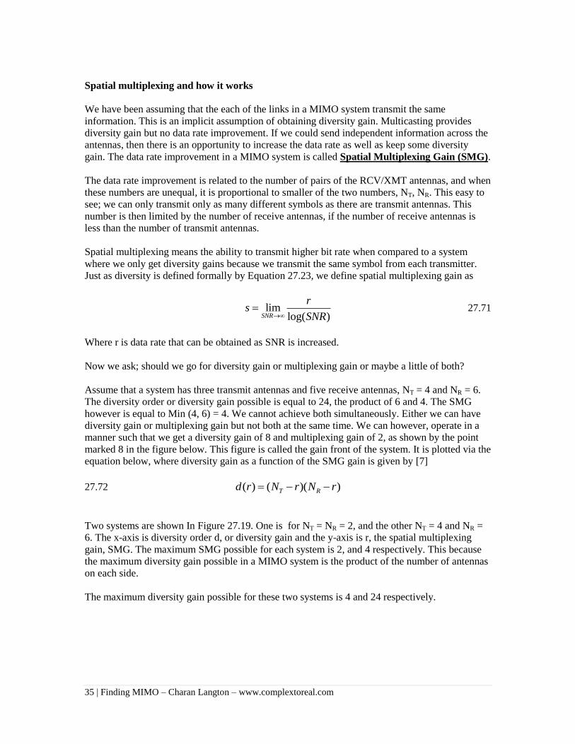
Assume that a system has three transmit antennas and five receive antennas, NT = 4 and NR = 6.
The diversity order or diversity gain possible is equal to 24, the product of 6 and 4. The SMG
however is equal to Min (4, 6) = 4. We cannot achieve both simultaneously. Either we can have
diversity gain or multiplexing gain but not both at the same time. We can however, operate in a
manner such that we get a diversity gain of 8 and multiplexing gain of 2, as shown by the point
marked 8 in the figure below. This figure is called the gain front of the system. It is plotted via the
equation below, where diversity gain as a function of the SMG gain is given by [7]
27.72 ( ) ( )( )T Rd r N r N r
Two systems are shown In Figure 27.19. One is for NT = NR = 2, and the other NT = 4 and NR =
6. The x-axis is diversity order d, or diversity gain and the y-axis is r, the spatial multiplexing
gain, SMG. The maximum SMG possible for each system is 2, and 4 respectively. This because
the maximum diversity gain possible in a MIMO system is the product of the number of antennas
on each side.
The maximum diversity gain possible for these two systems is 4 and 24 respectively.
36 | Finding MIMO – Charan Langton – www.complextoreal.com
24
15
8
4
0
4
100
4
8
12
16
20
24
0 1 2 3 4 5
Div
ers
ity
Gai
n,
d
Multiplexing Gain, r
(4x6)
(2x2)
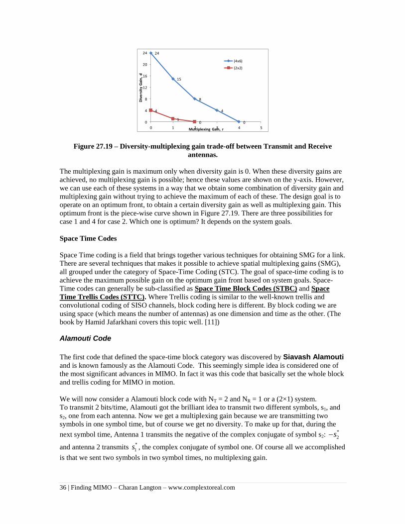
Figure 27.19 – Diversity-multiplexing gain trade-off between Transmit and Receive
antennas.
The multiplexing gain is maximum only when diversity gain is 0. When these diversity gains are
achieved, no multiplexing gain is possible; hence these values are shown on the y-axis. However,
we can use each of these systems in a way that we obtain some combination of diversity gain and
multiplexing gain without trying to achieve the maximum of each of these. The design goal is to
operate on an optimum front, to obtain a certain diversity gain as well as multiplexing gain. This
optimum front is the piece-wise curve shown in Figure 27.19. There are three possibilities for
case 1 and 4 for case 2. Which one is optimum? It depends on the system goals.
Space Time Codes
Space Time coding is a field that brings together various techniques for obtaining SMG for a link.
There are several techniques that makes it possible to achieve spatial multiplexing gains (SMG),
all grouped under the category of Space-Time Coding (STC). The goal of space-time coding is to
achieve the maximum possible gain on the optimum gain front based on system goals. Space-
Time codes can generally be sub-classified as Space Time Block Codes (STBC) and Space
Time Trellis Codes (STTC). Where Trellis coding is similar to the well-known trellis and
convolutional coding of SISO channels, block coding here is different. By block coding we are
using space (which means the number of antennas) as one dimension and time as the other. (The
book by Hamid Jafarkhani covers this topic well. [11])
Alamouti Code
The first code that defined the space-time block category was discovered by Siavash Alamouti and is known famously as the Alamouti Code. This seemingly simple idea is considered one of
the most significant advances in MIMO. In fact it was this code that basically set the whole block
and trellis coding for MIMO in motion.
We will now consider a Alamouti block code with NT = 2 and NR = 1 or a (2×1) system.
To transmit 2 bits/time, Alamouti got the brilliant idea to transmit two different symbols, s1, and
s2, one from each antenna. Now we get a multiplexing gain because we are transmitting two
symbols in one symbol time, but of course we get no diversity. To make up for that, during the
next symbol time, Antenna 1 transmits the negative of the complex conjugate of symbol s2: *
2s
and antenna 2 transmits *
1s , the complex conjugate of symbol one. Of course all we accomplished
is that we sent two symbols in two symbol times, no multiplexing gain.
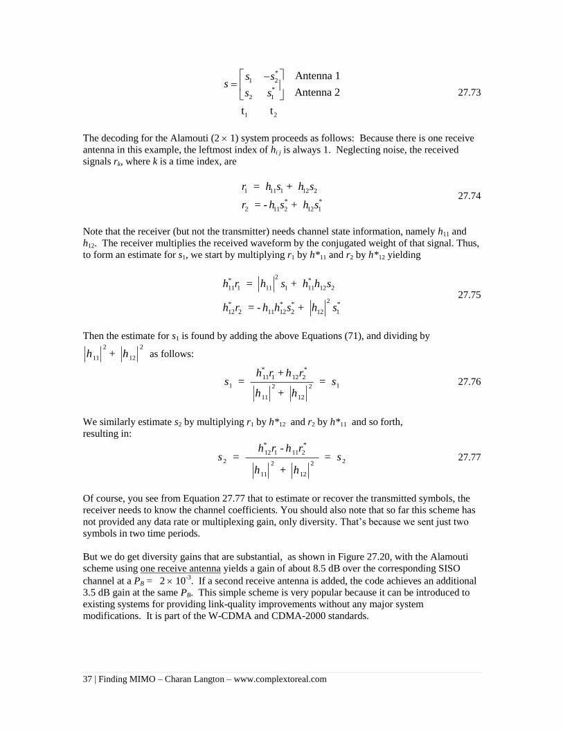
37 | Finding MIMO – Charan Langton – www.complextoreal.com
*
1 2
*
2 1
1 2
Antenna 1
Antenna 2
t t
s ss
s s
27.73
The decoding for the Alamouti (2 1) system proceeds as follows: Because there is one receive
antenna in this example, the leftmost index of hi j is always 1. Neglecting noise, the received
signals rk, where k is a time index, are
1 11 1 12 2
2 11 2 12 1
* *
r = h s + h s
r = - h s + h s 27.74
Note that the receiver (but not the transmitter) needs channel state information, namely h11 and
h12. The receiver multiplies the received waveform by the conjugated weight of that signal. Thus,
to form an estimate for s1, we start by multiplying r1 by h*11 and r2 by h*12 yielding
2
11 1 11 1 11 12 2
2
12 2 11 12 2 12 1
* *
* * * *
h r = h s + h h s
h r = - h h s + h s
27.75
Then the estimate for s1 is found by adding the above Equations (71), and dividing by 2 2
11 12h + h as follows:
11 1 12 2
1 12 2
11 12
* *h r +h rs = = s
h + h 27.76
We similarly estimate s2 by multiplying r1 by h*12 and r2 by h*11 and so forth,
resulting in:
12 1 11 2
2 22 2
11 12
* *h r - h rs = = s
h + h
27.77
Of course, you see from Equation 27.77 that to estimate or recover the transmitted symbols, the
receiver needs to know the channel coefficients. You should also note that so far this scheme has
not provided any data rate or multiplexing gain, only diversity. That’s because we sent just two
symbols in two time periods.
But we do get diversity gains that are substantial, as shown in Figure 27.20, with the Alamouti
scheme using one receive antenna yields a gain of about 8.5 dB over the corresponding SISO
channel at a PB = 2 10-3
. If a second receive antenna is added, the code achieves an additional
3.5 dB gain at the same PB. This simple scheme is very popular because it can be introduced to
existing systems for providing link-quality improvements without any major system
modifications. It is part of the W-CDMA and CDMA-2000 standards.
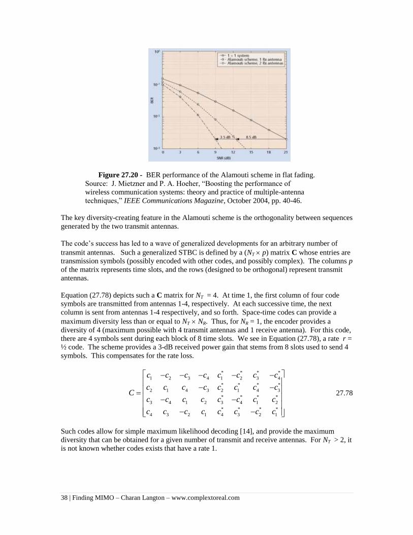
38 | Finding MIMO – Charan Langton – www.complextoreal.com
Figure 27.20 - BER performance of the Alamouti scheme in flat fading.
Source: J. Mietzner and P. A. Hoeher, “Boosting the performance of
wireless communication systems: theory and practice of multiple-antenna
techniques,” IEEE Communications Magazine, October 2004, pp. 40-46.
The key diversity-creating feature in the Alamouti scheme is the orthogonality between sequences
generated by the two transmit antennas.
The code’s success has led to a wave of generalized developments for an arbitrary number of
transmit antennas. Such a generalized STBC is defined by a (NT p) matrix C whose entries are
transmission symbols (possibly encoded with other codes, and possibly complex). The columns p
of the matrix represents time slots, and the rows (designed to be orthogonal) represent transmit
antennas.
Equation (27.78) depicts such a C matrix for NT = 4. At time 1, the first column of four code
symbols are transmitted from antennas 1-4, respectively. At each successive time, the next
column is sent from antennas 1-4 respectively, and so forth. Space-time codes can provide a
maximum diversity less than or equal to NT NR. Thus, for NR = 1, the encoder provides a
diversity of 4 (maximum possible with 4 transmit antennas and 1 receive antenna). For this code,
there are 4 symbols sent during each block of 8 time slots. We see in Equation (27.78), a rate r =
½ code. The scheme provides a 3-dB received power gain that stems from 8 slots used to send 4
symbols. This compensates for the rate loss.
* * * *
1 2 3 4 1 2 3 4
* * * *
2 1 4 3 2 1 4 3
* * * *
3 4 1 2 3 4 1 2
* * * *
4 3 2 1 4 3 2 1
c c c c c c c c
c c c c c c c cC
c c c c c c c c
c c c c c c c c
27.78
Such codes allow for simple maximum likelihood decoding [14], and provide the maximum
diversity that can be obtained for a given number of transmit and receive antennas. For NT > 2, it
is not known whether codes exists that have a rate 1.
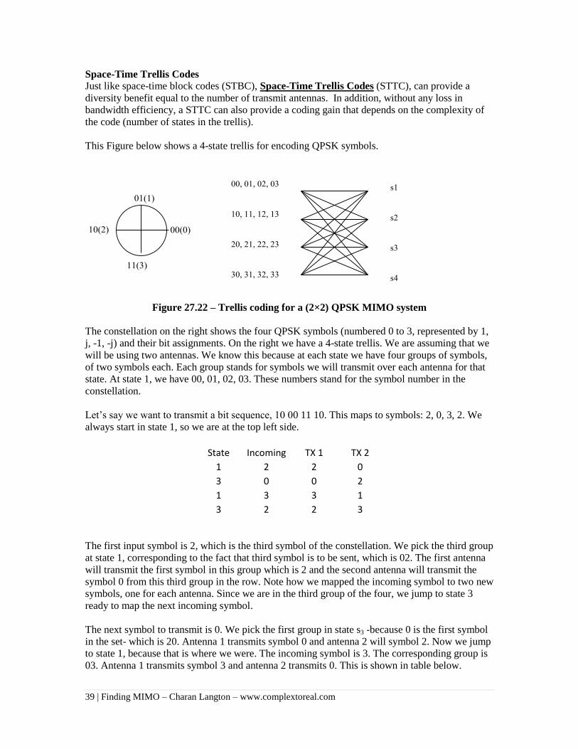
39 | Finding MIMO – Charan Langton – www.complextoreal.com
Space-Time Trellis Codes Just like space-time block codes (STBC), Space-Time Trellis Codes (STTC), can provide a
diversity benefit equal to the number of transmit antennas. In addition, without any loss in
bandwidth efficiency, a STTC can also provide a coding gain that depends on the complexity of
the code (number of states in the trellis).
This Figure below shows a 4-state trellis for encoding QPSK symbols.
Figure 27.22 – Trellis coding for a (2×2) QPSK MIMO system
The constellation on the right shows the four QPSK symbols (numbered 0 to 3, represented by 1,
j, -1, -j) and their bit assignments. On the right we have a 4-state trellis. We are assuming that we
will be using two antennas. We know this because at each state we have four groups of symbols,
of two symbols each. Each group stands for symbols we will transmit over each antenna for that
state. At state 1, we have 00, 01, 02, 03. These numbers stand for the symbol number in the
constellation.
Let’s say we want to transmit a bit sequence, 10 00 11 10. This maps to symbols: 2, 0, 3, 2. We
always start in state 1, so we are at the top left side.
State Incoming TX 1 TX 2
1 2 2 0
3 0 0 2
1 3 3 1
3 2 2 3
The first input symbol is 2, which is the third symbol of the constellation. We pick the third group
at state 1, corresponding to the fact that third symbol is to be sent, which is 02. The first antenna
will transmit the first symbol in this group which is 2 and the second antenna will transmit the
symbol 0 from this third group in the row. Note how we mapped the incoming symbol to two new
symbols, one for each antenna. Since we are in the third group of the four, we jump to state 3
ready to map the next incoming symbol.
The next symbol to transmit is 0. We pick the first group in state s3 -because 0 is the first symbol
in the set- which is 20. Antenna 1 transmits symbol 0 and antenna 2 will symbol 2. Now we jump
to state 1, because that is where we were. The incoming symbol is 3. The corresponding group is
03. Antenna 1 transmits symbol 3 and antenna 2 transmits 0. This is shown in table below.
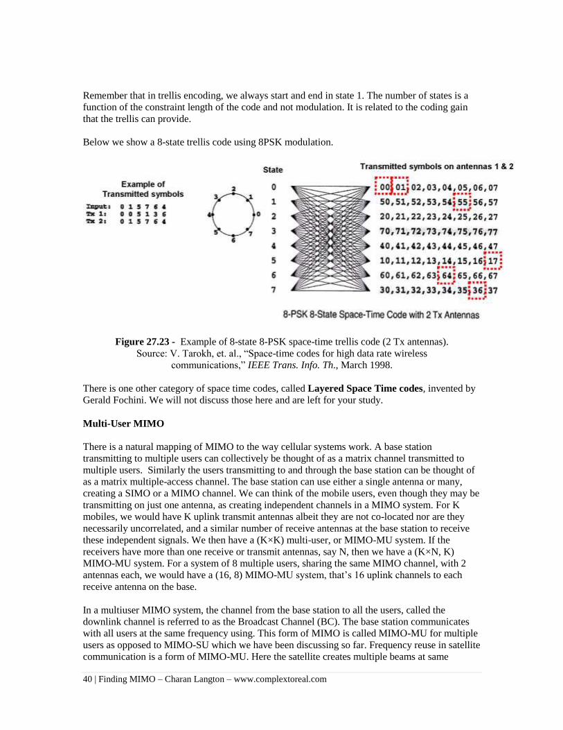
40 | Finding MIMO – Charan Langton – www.complextoreal.com
Remember that in trellis encoding, we always start and end in state 1. The number of states is a
function of the constraint length of the code and not modulation. It is related to the coding gain
that the trellis can provide.
Below we show a 8-state trellis code using 8PSK modulation.
Figure 27.23 - Example of 8-state 8-PSK space-time trellis code (2 Tx antennas).
Source: V. Tarokh, et. al., “Space-time codes for high data rate wireless
communications,” IEEE Trans. Info. Th., March 1998.
There is one other category of space time codes, called Layered Space Time codes, invented by
Gerald Fochini. We will not discuss those here and are left for your study.
Multi-User MIMO
There is a natural mapping of MIMO to the way cellular systems work. A base station
transmitting to multiple users can collectively be thought of as a matrix channel transmitted to
multiple users. Similarly the users transmitting to and through the base station can be thought of
as a matrix multiple-access channel. The base station can use either a single antenna or many,
creating a SIMO or a MIMO channel. We can think of the mobile users, even though they may be
transmitting on just one antenna, as creating independent channels in a MIMO system. For K
mobiles, we would have K uplink transmit antennas albeit they are not co-located nor are they
necessarily uncorrelated, and a similar number of receive antennas at the base station to receive
these independent signals. We then have a (K×K) multi-user, or MIMO-MU system. If the
receivers have more than one receive or transmit antennas, say N, then we have a (K×N, K)
MIMO-MU system. For a system of 8 multiple users, sharing the same MIMO channel, with 2
antennas each, we would have a (16, 8) MIMO-MU system, that’s 16 uplink channels to each
receive antenna on the base.
In a multiuser MIMO system, the channel from the base station to all the users, called the
downlink channel is referred to as the Broadcast Channel (BC). The base station communicates
with all users at the same frequency using. This form of MIMO is called MIMO-MU for multiple
users as opposed to MIMO-SU which we have been discussing so far. Frequency reuse in satellite
communication is a form of MIMO-MU. Here the satellite creates multiple beams at same
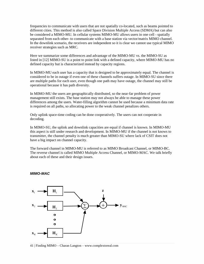
41 | Finding MIMO – Charan Langton – www.complextoreal.com
frequencies to communicate with users that are not spatially co-located, such as beams pointed to
different cities. This method is also called Space Division Multiple Access (SDMA) but can also
be considered a MIMO-MU. In cellular systems MIMO-MU allows users in one cell - spatially
separated from each other- to communicate with a base station via vector/matrix MIMO channel.
In the downlink scenario, the receivers are independent so it is clear we cannot use typical MIMO
receiver strategies such as MRC.
Here we summarize some differences and advantage of the MIMO-MU vs. the MIMO-SU as
listed in [12] MIMO-SU is a point to point link with a defined capacity, where MIMO-MU has no
defined capacity but is characterized instead by capacity regions.
In MIMO-MU each user has a capacity that is designed to be approximately equal. The channel is
considered to be in outage if even one of these channels suffers outage. In MIMO-SU since there
are multiple paths for each user, even though one path may have outage, the channel may still be
operational because it has path diversity.
In MIMO-MU the users are geographically distributed, so the near-far problem of power
management still exists. The base station may not always be able to manage these power
differences among the users. Water-filling algorithm cannot be used because a minimum data rate
is required on all paths, so allocating power to the weak channel penalizes others.
Only uplink space-time coding can be done cooperatively. The users can not cooperate in
decoding.
In MIMO-SU, the uplink and downlink capacities are equal if channel is known. In MIMO-MU
this aspect is still under research and development. In MIMO-MU if the channel is not knows to
transmitter, the channel penalty is much greater than MIMO-SU where lack of CSIT does not
have a big impact on channel capacity.
The forward channel in MIMO-MU is referred to as MIMO Broadcast Channel, or MIMO-BC.
The reverse channel is called MIMO Multiple Access Channel, or MIMO-MAC. We talk briefly
about each of these and their design issues.
MIMO-MAC
1H z
MACy2H
KH
1x
2x
Kx
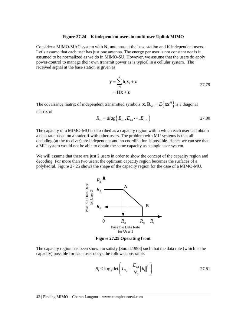
42 | Finding MIMO – Charan Langton – www.complextoreal.com
Figure 27.24 – K independent users in multi-user Uplink MIMO
Consider a MIMO-MAC system with NT antennas at the base station and K independent users.
Let’s assume that each user has just one antenna. The energy per user is not constant nor is it
assumed to be normalized as we do in MIMO-SU. However, we assume that the users do apply
power-control to manage their own transmit power as is typical in a cellular system. The
received signal at the base station is given as
1
K
i i
i
y h x z
Hx + z
27.79
The covariance matrix of independent transmitted symbols , H
xx Ex R xx is a diagonal
matrix of
,1 ,1 ,, ,ss s s s KR diag E E E 27.80
The capacity of a MIMO-MU is described as a capacity region within which each user can obtain
a data rate based on a tradeoff with other users. The problem with MU systems is that all
decoding (at the receiver) are independent and no coordination is possible. Hence we can see that
a MU system would not be able to obtain the same capacity as a single user system.
We will assume that there are just 2 users in order to show the concept of the capacity region and
decoding. For more than two users, the optimum capacity region becomes the surfaces of a
polyhedral. Figure 27.25 shows the shape of the capacity region for the case of a MIMO-MU.
Figure 27.25 Operating front
The capacity region has been shown to satisfy [Surad,1998] such that the data rate (which is the
capacity) possible for each user obeys the follows constraints
2,1
1 2 1
0
log detB
s
N
ER I h
N
27.81
2R
1R
Possible Data Rate
for User 1
A
B
AR BR
BR
AR
Poss
ible
Data
Rate
for
Use
r 2
0
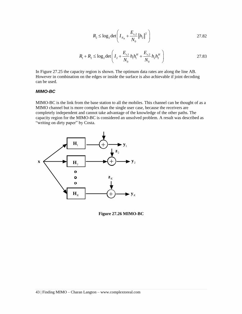
43 | Finding MIMO – Charan Langton – www.complextoreal.com
2,2
2 2 2
0
log detB
s
N
ER I h
N
27.82
,1 ,2
1 2 2 2 1 1 2 2
0 0
log dets sH H
E ER R I h h h h
N N
27.83
In Figure 27.25 the capacity region is shown. The optimum data rates are along the line AB.
However in combination on the edges or inside the surface is also achievable if joint decoding
can be used.
MIMO-BC
MIMO-BC is the link from the base station to all the mobiles. This channel can be thought of as a
MIMO channel but is more complex than the single user case, because the receivers are
completely independent and cannot take advantage of the knowledge of the other paths. The
capacity region for the MIMO-BC is considered an unsolved problem. A result was described as
“writing on dirty paper” by Costa.
1H1y
2H
KH
x
2y
Ky
2z
Kz
Figure 27.26 MIMO-BC
44 | Finding MIMO – Charan Langton – www.complextoreal.com
References
1. On limits of wireless communications in a fading environment when using multiple
antennas. G. Foschini, M. Ganns. 1998, Wireless Personal Comminications, pp. 311-
335.
2. A Mathematical Theory of Communications. Shannon, C. E. Vols. Bell Systems
Technical Journal, vol. 27, 1948, pp. 379-423 and 623-656.
3. Capacity of Multiantenna Gaussian Channels. Telatar, E. s.l. : European Transactions
on Telecommunications, , November/December 1999, Vols. vol. 10, No. 6, pp.585-595.
4. On limits of wireless communications in a fading environment when using multiple
antennas. Gans, G. J. Foschini and M. J. 1998, Vols. Wireless Personal
Communications, vol. 6, 1998, pp. 311-335.
5. Receive and Transmit Array Antenna Spacing and Their Effect on the Performance of
SIMO and MIMO Systems by using an RCS Channel. N. Ebrahimi-Tofighi, M.
ArdebiliPour, and M. Shahabadi. 2007, World Academy of Science, Engineering and
Technology , p. 36.
6. Costa, Nelson and Haykin Simon. “Multiple-Input Multiple-Output Channel
Models” . s.l. : John Wiley, 2010.
7. D. Tse, Pramod Viswanth. Fundamental of Wireless Communications. s.l. :
Cambridge University Press, 2005.
8. Proakis, J. G. Digital Communications. New York : McGraw Hill Book Co., 2000 4th
Edition.
9. Sklar, Bernard. Digital Communications. s.l. : Prentice Hall.
10. Goldsmith, A. Wireless Communications.
11. Jafarkhani, Hamid. Space-Time Cding. s.l. : Cambridge University Press, 2005.
12. Arogoyasami, Nabar, Gore 2003. Space-Time Coding. s.l. : Cambridge University
press, 2005.
13. From Theory to Practice: An Overview of MIMO. David Gesbert, Mansoor shafi,
Peter J. Smith, Ayman Nagui, Da-shan Shiu. s.l. : IEEE Journal of Selected Topics in
Communications, 2003, Vols. Vol 21, No. 3.
14. Yong Soo-Cho, Won Young Yan. MIMO-OFDM Wireless Communications with
Matlab. s.l. : IEEE Press, John Wiley and Sons, 2010.
15. Goldsmith, Andrea, Wireless Communication, 1. Hottinen, A, Trikkonen Olav,
Wichman, Rist. Multi-antenna Transceiver Techniques for 3G and Beyond. s.l. : John
Wiley & Sons, 2003.
16. Branka Vucetic, Jinhong Yan. Space – Time Coding. s.l. : John Wiley, 2003.
17. Arogyaswami Pulraj, Rohit Nabr, Dhananjay Gore. Introduction of Space-Time
Wireless Communications . s.l. : Cambridge University Press, 2003.
18. A simple transmit diversity technique for wireless communications. Alamouti, S. M.
s.l. : IEEE J. on Selected Areas in Communications, Vols. vol. 16, no. 8, October 1998,
pp. 1451-1458.
19. Layered space–time architecture for wireless communication in a fading environment
when using multiple antennas. Foschini, G. J. s.l. : Bell Labs Syst. Tech. J., vol. 1, p. 41–
59, Autumn 1996.

45 | Finding MIMO – Charan Langton – www.complextoreal.com
Bibliographic Notes
In the writing of this paper, I relied heavily on some books and papers. The three books I
often found myself thumbing through, in order are: Wireless Communications by Andrea
Goldsmith, Fundamentals of Wireless Communications by D. Tse and P. Viswanath and
Digital Communications by Proakis, 5th Edition. The examples used in this paper are inspired
by the Andrea Goldsmith book, the one I consider the best. She has a lot of examples in her
book which truly help with understanding.
The other three books that I also found helpful were: Digital Communications by Barry, Less
and Messerschmitt, Introduction to Space-Time Wireless Communications by Paulraj, Nabar
and Gore and MIMO-OFDM Wireless Communications with Matlab book by Yong
Soo-Cho, and Won Young Yan. I used the Matlab code in this book to create some of
the capacity graphs.
With papers, the one I read several times was by Gesbert’s [13] and the one by Foschini. [1] I
read many others but these two stand out. Agilent also has an excellent tutorial online. And of
course the David Tse video lecture is fantastic. IEEE also has an audio lecture that is
excellent.
It took me a while to get all my ideas together and I read many papers and checked nearly all
the books written on the topic. While writing about these, I often could not figure out who the
original source was. This is not good as I do want to credit to whom it is is due. If you the
reader feel that I have not properly credited you or someone else in this paper, please do let
me know.
In writing, Bernard wrote the first draft and then I added and subtracted from it. The paper is
now nearly 50 pages but it is still lacking in many areas. I was not able to cover STC
decoding, nor the code performance issues. The section on multi-user is also short. But I hope
that what is here will help illuminate the topic and get you started.
This paper copyright by Charan Langton 2011
All rights Reserved.
For an up-to-date copy of this tutorial, please check www.complextoral.com