Cold-water coral reefs and adjacent sponge grounds ... · PDF fileCold-water corals and sponges form complex reef structures on the seaﬂoor (Figure1), which support a rich community

ORIGINAL RESEARCHpublished: 19 June 2015

doi: 10.3389/fmars.2015.00037

Frontiers in Marine Science | www.frontiersin.org 1 June 2015 | Volume 2 | Article 37

Edited by:

Hajime Kayanne,

The University of Tokyo, Japan

Reviewed by:

Aldo Cróquer,

Simon Bolivar University, Venezuela

Toshihiro Miyajima,

The University of Tokyo, Japan

*Correspondence:

Cécile Cathalot,

Laboratory of Geochemistry and

Metallogeny, Ifremer (Brest), ZI de la

Pointe du Diable, CS10070, F-29280

Plouzané, France

[email protected]

Specialty section:

This article was submitted to

Coral Reef Research,

a section of the journal

Frontiers in Marine Science

Received: 18 December 2014

Accepted: 23 May 2015

Published: 19 June 2015

Citation:

Cathalot C, Van Oevelen D, Cox TJS,

Kutti T, Lavaleye M, Duineveld G and

Meysman FJR (2015) Cold-water

coral reefs and adjacent sponge

grounds: hotspots of benthic

respiration and organic carbon cycling

in the deep sea. Front. Mar. Sci. 2:37.

doi: 10.3389/fmars.2015.00037

Cold-water coral reefs and adjacentsponge grounds: hotspots of benthicrespiration and organic carboncycling in the deep sea

Cécile Cathalot 1*, Dick Van Oevelen 1, Tom J. S. Cox 1, 2, Tina Kutti 3, Marc Lavaleye 4,

Gerard Duineveld 4 and Filip J. R. Meysman 1, 5

1Department of Ecosystem Studies, Royal Netherlands Institute for Sea Research, Yerseke, Netherlands, 2 Ecosystem

Management Research Group, Universiteit Antwerpen, Wilrijk, Belgium, 3Department of Benthic Resources and Processes,

Institute of Marine Research, Bergen, Norway, 4Department of Marine Ecology, Royal Netherlands Institute for Sea Research,

Den Burg, Netherlands, 5 Laboratory of Analytical, Environmental and Geochemistry, Vrije Universiteit Brussel, Brussels,

Belgium

Cold-water coral reefs and adjacent sponge grounds are distributed widely in the deep

ocean, where only a small fraction of the surface productivity reaches the seafloor

as detritus. It remains elusive how these hotspots of biodiversity can thrive in such

a food-limited environment, as data on energy flow and organic carbon utilization are

critically lacking. Here we report in situ community respiration rates for cold-water

coral and sponge ecosystems obtained by the non-invasive aquatic Eddy Correlation

technique. Oxygen uptake rates over coral reefs and adjacent sponge grounds in the

Træna Coral Field (Norway) were 9–20 times higher than those of the surrounding soft

sediments. These high respiration rates indicate strong organic matter consumption, and

hence suggest a local focusing onto these ecosystems of the downward flux of organic

matter that is exported from the surface ocean. Overall, our results show that coral reefs

and adjacent sponge grounds are hotspots of carbon processing in the food-limited

deep ocean, and that these deep-sea ecosystems play a more prominent role in marine

biogeochemical cycles than previously recognized.

Keywords: deep-sea ecosystems, cold-water corals, sponges, respiration, energy flow

Introduction

Cold-water corals and sponges form complex reef structures on the seafloor (Figure 1),which support a rich community of suspension-feeding fauna and play a crucial role asa refuge, feeding ground and nursery for various commercial fishes (Miller et al., 2012).These reef ecosystems are widespread across the deep ocean (Klitgaard and Tendal, 2004;Roberts et al., 2006), but they face an uncertain future, as the human imprint on thedeep-sea rapidly increases (Pusceddu et al., 2014). As oil and gas exploration are movinginto deeper waters, seafloor installations, accidental oil spilling and sediment plumes areincreasingly impacting the reef structures (Purser and Thomsen, 2012; Fisher et al., 2014;Roberts and Cairns, 2014), while physical disturbance by intensified bottom trawling significantlydamages the slow growing reefs (Fossa et al., 2002; Althaus et al., 2009; Miller et al., 2012).

http://www.frontiersin.org/Marine_Science

http://www.frontiersin.org/Marine_Science/editorialboard




http://dx.doi.org/10.3389/fmars.2015.00037


http://www.frontiersin.org

http://www.frontiersin.org/Marine_Science/archive

https://creativecommons.org/licenses/by/4.0/

mailto:[email protected]

http://dx.doi.org/10.3389/fmars.2015.00037

http://journal.frontiersin.org/article/10.3389/fmars.2015.00037/abstract

http://community.frontiersin.org/people/u/200270







Cathalot et al. Coral reefs and sponges respiration

FIGURE 1 | (A) Bathymetry map of the Træna Deep Coral reef field with red

dots representing known cold-water coral reef locations. (B) Sampling sites:

two reefs were investigated and the symbols mark the locations of AqEC

deployments. (C) Topography of Reef R1. The location of the AqEC

deployment is indicated by the gray arrow. The size of the upstream AqEC

footprint area, as indicated by the oval shape above the reef, was estimated

using the equations in Berg et al. (2007) using the cross correlation among

the 3D velocity components to calculate the friction velocity. (D) Photograph

of a vertical lobe of densely packed branches of living Lophelia pertusa at the

head of Reef R1. The exact position is indicated by the red square in (C). (E)

Coral branch sampled by ROV Aglantha. The shaded area indicates the

planar view that can be “seen” by the ROV camera. The underlying layers of

living and dead polyps remain hidden from the camera’s view and are

indicated by the accolade.

Cold-water coral ecosystems are also considered to be stronglysensitive to various impacts of climate change. Foremost, oceanacidification is considered amajor threat to their future existence,due to the anticipated shoaling of aragonite saturation horizonand the associated reduction in calcification rates (Roberts andCairns, 2014). Energy availability is considered a prime factorin the sensitivity of cold-water corals to ocean acidification, andtherefore, climate-induced shifts in the primary production andexport from the surface ocean should also be considered. Asrising sea-surface temperatures can reduce water column mixingand intensify the recycling of organic matter in the surfaceocean, climate change can decrease the carbon export flux tothe deep sea (Bopp et al., 2001). Moreover, the energy demands

and respiration rates of the reef-forming species are predictedto increase in a warmer ocean (Dodds et al., 2007; Roberts andCairns, 2014), thus aggravating the food limitation problem.While the sensitivity to ocean acidification is increasinglyaddressed in experimental andmodeling studies, it is unclear howthese climate-induced changes in food supply and respiration willaffect the ecosystem functioning of cold-water coral and spongecommunities. To resolve this, data on the energy flow and organiccarbon (OC) processing rates within these deep-sea ecosystemsare critically needed.

A recent food web model analysis from the Logachev Moundcomplex (NE Atlantic) suggests that OC processing rates inCold-Water Coral Reefs (CWCR) largely exceed those of the






surrounding soft sediments (Van Oevelen et al., 2009). Moreover,Kutti et al. (2013) estimated that reef-associated sponge groundscan also process considerable amounts of OC, based on spongeabundance data and laboratory-based respiration rates. Yet, untilnow, there has been no experimental in situ validation of this“high OC processing” hypothesis. Community respiration ratesin reef environments are difficult to quantify, as the diversityof fauna, habitat complexity and up-scaling issues preventthe use of traditional techniques (e.g., incubation chambers,microsensor profiling). Here we report in situ measurements ofcommunity respiration rates for CWCR and adjacent spongegrounds, obtained by Aquatic Eddy Correlation (AqEC), whichis a novel technique that allows the in situ determination ofcommunity respiration rates in topographically complex seafloorenvironments (Berg et al., 2003; Lorrai et al., 2010; Long et al.,2013; Attard et al., 2014). The AqEC technique is non-invasive,and integrates the benthic oxygen flux over a large footprint area(>10m2, Berg et al., 2007). Our data show that carbon processingin CWCR and associated sponge grounds is much more intensethan previously recognized: these ecosystems not only act ashavens of biodiversity, but are true hotspots of organic carboncycling in a food-limited deep sea.

Materials and Methods

Study Site and SamplingData were collected in May 2011 on board R/V Håkon Mosby,on a cruise to the Træna Marine Protected Area (MPA),which covers 300 km2 of the Norwegian continental margin.The seafloor in the Træna Deep Coral reef field (Norwegiancontinental shelf) consists of three main habitat types (Buhl-Mortensen et al., 2010; Kutti et al., 2013): (i) elongated, cigar-shaped reefs (100–150m long, 25–55m wide and on average7m high) formed by the reef-building coral Lophelia pertusa,(ii) dense sponge grounds surrounding the coral reefs, consistingof aggregations of large demosponges, and (iii) stretchesof bare sediment, containing typical soft-sediment infauna,

which are located further away from the reefs and spongegrounds.

We performed three types of data collection (Table 1): (i)Aquatic Eddy Correlation (AqEC) lander deployments to obtainin situ Community Respiration (CR) rates, (ii) Smøgen box-corer deployments to retrieve soft sediment, living coral branchesand dead coral branches for shipboard incubations, and (iii)dives with the Remotely Operated Vehicle (ROV) Aglantha tocollect branches of living coral and samples of living sponges,and to obtain video footage for seafloor habitat mapping andestimates of coral and sponge densities. Deployments were doneat five different locations: two reefs (R1 and R2), their associatedsurrounding sponge grounds (S1 and S2), and one control sitewith bare soft sediments (C). The control site did not host coralsor sponges, and was located at a similar water depth, east of theTræna Coral MPA (Figure 1B).

CWCR in the Træna area are aligned along themain westwardcurrent direction (Laberg et al., 2002) and are typically composedof three distinct parts: a “head” part with living coral, a “middle”section with dead coral framework, and a long “tail” part,which consists primarily of coral rubble (Figure 1C). The reef ’shead part faces the current and consists of several meters widevertically-oriented lobes, primarily composed of living Lopheliapertusa, (Buhl-Mortensen et al., 2010, Figure 2D). The spongeground sites were located in the vicinity of the reef sites and weredominated by three sponge types:Mycale lingua, Oceanapia spp.,and Geodiidea (Kutti et al., 2013).

Biological Data on Corals and SpongesWedetermined the coral polyp density fromROV video transectsat site R1 (Table 2) along three different lobes of live Lophelia.The number of “visible” polyps per square meter was estimatedon calibrated (i.e., corrected for the view angle of the camera)still images taken from the video. To this end, we delineated 3–4squares of 10 cm by 10 cm in a single video image and countedthe number of “visible” polyps within these reference squares.

By comparing the number of living polyps on intact coralbranches collected by the ROV with the number of living polyps

TABLE 1 | Station locations and instrument deployments.

Date Longitude (◦W) Latitude (◦N) Type of habitat Instrument Type of measurement

27.05.2011 11 ◦ 26.27 66 ◦ 56.13 Bare sediment AqEC In situ CR

27.05.2011 11 ◦ 26.72 66 ◦ 56.35 Bare sediment Box corer 3 onboard incubations of sediment cores

28.05.2011 11 ◦ 07.76 66 ◦ 58.31 Coral reef R1 ROV Sampling of Lophelia branches followed by on-board incubation

28.05.2011 11 ◦ 07.95 66 ◦ 58.44 Coral reef R1 Box corer 3 core incubations

29.05.2011 11 ◦ 05.94 66 ◦ 58.44 Coral reef R1 AqEC In situ CR

29.05.2011 10 ◦ 58.45 66 ◦ 58.20 Sponge groundS1 ROV Geodia collection + incubation


29.05.2011 11 ◦ 06.12 66 ◦ 58.44 Sponge ground S1 AqEC In situ CR

29.05.2001 11 ◦ 06.48 66 ◦ 58.44 Coral reef R2 AqEC In situ CR

29.05.2011 11 ◦ 06.12 66 ◦ 58.44 Sponge ground S1 Box corer 2 core incubations

30.05.2011 11 ◦ 06.66 66 ◦ 58.44 Sponge ground S2 AqEC In situ CR


30.05.2011 11 ◦ 06.66 66 ◦ 58.44 Sponge ground S2 Box corer 2 core incubations

AqEC, Aquatic Eddy Correlation; CR, Community Respiration; ROV, Remotely Operated Vehicle.






FIGURE 2 | AqEC correlation data for consecutive 15min bursts

during the deployment at the reef R1, sponge ground and bare

sediment sites. (A) Velocity data (x, y, z) after a 3Hz low-pass filtering.

(B) Raw O2 concentration data after a 3Hz low-pass filtering. (C) Derived O2

flux for each burst (rectangles). (D) Images of the corresponding habitats and

associated communities (Cold water coral, sponges and bare sediment).

that were visible on single branches in calibrated ROV videoimages, we estimated that 80 ± 10% of the living polyps werehidden from view on the ROV video images (Figure 1E). Wehence multiplied the “visible” polyp density estimated from theROV video images by a factor of 5 to arrive at the true arealdensity of living L. pertusa polyps.

We estimated the abundance of the fourmain sponges (Geodiabarretti, G. atlantica, G. macandrewii, and other Porifera) byanalyzing images of an ROV survey (HL5-5) carried out in 2009at site S1 (Kutti et al., 2013). In each image, individual spongeswere taxonomically identified and their density (ind m−2) andindividual size (length, diameter) was estimated.

In addition, a scaling relation was derived between the volumeand biomass of Geodia barretti (Table 3) to estimate the totalsponge biomass. During the cruise, five specimen of G. barrettiwere collected with the ROV, and their individual volume(through water displacement) and wet weight was measured.Dry weight biomass was calculated from wet weight using a0.2 conversion factor determined from previous measurementson Geodia sponges (Tjensvoll et al., 2013; Kutti et al.,2014).

Eddy Correlation in situ Community RespirationMeasurementsFive deployments were performed within the three habitat types(1 in soft-sediment, 2 in sponge ground and 2 in coral reefhabitat) using a tripod lander, which carried the Aquatic EddyCovariance (AqEC) instrument and which was launched fromthe research vessel (Table 1). The AqEC flux technique is basedon the simultaneous high-frequency measurement of the currentvelocity vector u and the oxygen concentration C at a given heightabove the seabed, from which the turbulent fluctuations in theoxygen concentration C′ and in vertical current velocity u’z arecalculated. The oxygen flux toward the seabed is subsequentlyobtained as the temporal average of the covariance u′z C′ (Berget al., 2003, 2009). The AqEC instrument consisted of anAcoustic Doppler Velocimeter (ADV, Vector Nortek R©) and afast-responding Clark-type O2 microelectrode directly connectedto an auto-zeroing amplifier (Unisense R©, Denmark). Both theADV and the O2 sensor were interfaced to a controller unit(Unisense R©, Denmark), which took care of power supply, sensorsynchronization and data storage. The O2 sensors (Unisense R©,Denmark) had an outer tip diameter of ∼5µm, and a response






time of ∼0.3 s. The O2 sensor was polarized for at least 6 h priorto use and a two-point calibrated was carried out using saturatedbottom water (100% reference) and an oxygen-free solution of1M Na-ascorbate and 0.5M NaOH (0% reference).

The AqEC instrument was mounted on a tripod bottomlander equipped with a vane attached to one leg of the lander,which ensured that the O2 sensor faced the direction ofthe main current (Figure 1). Visual inspection by the ROVconfirmed the correct positioning of the AqEC lander on the reefframework. In all deployments, the sensor volume of the ADVwas positioned 35–45 cm above the sediment-water interface.AqEC deployments typically lasted 2 h, except for the deploymentin the bare sediment control area, which lasted 24 h. During this24 h deployment, we selected 2 h (8 bursts) of data that passedquality control criteria (see details below). Data collection alwaysproceeded in 15min bursts, each consisting of a 14min period ofdata recording at 64Hz, followed by a 1min pause.

TABLE 2 | Polyp density of Reef R1 based on ROV video survey images.

Lobe No. of polyps on image No. of polyps

per 10 × 10cm2 area m−2

1 23 1668

1 35 2538

1 33 2393

1 32 2320

2 36 2610

2 26 1885

2 36 2610

3 30 2175

3 40 2900 Considering 5

layers of polyps3 40 2900

Average 33.1 ± 5.6 2400 ± 400 12000 ± 2000

n.b., Number of polyps were estimated based on calibrated snapshots (factor: 0.725).

AqEC data time series were pre-processed using a dedicatedR script developed at NIOZ, which involved de-spiking of theoxygen and velocity data, followed by a two-axis rotation ofthe velocity data (Mcginnis et al., 2008). In case of the reefdeployments, we applied a planar fit rotation to the velocity datain order not to make any further assumptions on the flow field,and to examine the occurrence of any flow divergence that mightgenerate spurious fluxes. A low-pass filter (3Hz) was appliedto the vertical velocity data to remove high-frequency noise. Inoceanic environments, flux contributions are typically below 1Hz(Lorrai et al., 2010), and we verified that our low-pass filtering didnot affect the calculated fluxes.

In AqEC studies, three methods have been used to obtain thefluctuating components of the vertical velocity and oxygen (meanremoval, linear detrending, and running mean filtering). In thisstudy, we implemented runningmean filtering because it gave thebest linear cumulative fluxes (please see below). To this end, themean velocity and oxygen concentration were calculated as therunning means obtained by applying a 1/60Hz high-pass filter tothe 3Hz filtered data in each burst. Referring to these runningmeans as uz and Cz , values of u′z and C′ were then calculated asuz – uz and C – Cz where uz and C represent the 3Hz filtereddata. The AqEC flux was then calculated as the mean covarianceover the time domain of each burst together with the associatedcumulative flux. The cumulative flux is simply the value of theinstantaneous AqEc flux (u′zC

′), which is integrated over time.If u′zC

′ is constant in time, this cumulative flux should increasein a linear way throughout each burst. Hence, the cumulativeflux was visually inspected to reflect a steady linear uptake of O2

by the seafloor during the respective bursts. If the cumulativeflux did not display a sufficiently linear trend (r2 < 0.6), theburst was discarded. A fast Fourier transformation of u′z andC′ provides the individual spectra as well as the co-spectrum,which expresses the flux contribution as a function of the eddyfrequency (Berg et al., 2003). After careful examination of thevariance preserving co-spectra of each burst, the use of a 60 saveraging time period was selected (i.e., 1/60Hz high-pass filter

TABLE 3 | Estimation of the sponge density and biomass from ROV video survey images and of respiration rates.

Average density Average Biomass* Biomass § Respiration CR

Diameter rates† rates

(ind m−2) (cm) (kg WW m−2) (kg DW m−2) (mmolO2 g DW d−1) (mmolO2 m−2 d−1)

Geodia barretti 0.24 29 3.2 ± 1.5 0.63 ± 0.3 0.036 23.0 ± 10.8

G. atlantica 0.07 53 0.8 ± 0.4 0.16 ± 0.08 0.036 5.8 ± 2.9

G. macandrewii 0.02 24 0.3 ± 0.1 0.06 ± 0.02 0.036 2.2 ± 0.7

Porifera indet. 0.22 19 2 ± 0.9 0.4 ± 0.2 0.036 14.4 ± 6.5

Total community of massive sponges 0.55 6.3 ± 2.9 1.3 ± 0.6 0.036 45.3 ± 20.9

Sponge sediment 3.4 ± 0.6

Total 48.7 ± 21.5

*Biomass was calculated for each individual using the size-weight conversion factor measured for G. barretti, i.e., biomass = 0.0003 × length3 (Kutti et al., 2013). §Conversion factor

of 0.20 was used to convert from wet weight to dry weight biomass. †The respiration rate obtained for G. barretti was used also to estimate oxygen consumption of the other massive

sponges.






as noted above) ensuring that the lowest frequencies contributingto the flux are accounted for.

Quality control of the AqEC time series data is crucial foraccurate flux extraction. Each burst was examined separatelyand the burst data were discarded if (1) ADV data were ofinsufficient quality (beam correlation values below 70%), (2) thecurrent velocity and oxygen concentration showed any sign ofstatistical non-stationarity (by investigating changes in the meanand standard deviation of C and uz over time) or (3) storageeffects were noted (by monitoring the oxygen inventory betweensediment and the O2 sensor position) (4) the cumulative fluxwas not sufficiently linear (Reba et al., 2009; Hume et al., 2011;Lorke et al., 2013). Hence, the entire 2 h data-sets for the reefsand sponges deployments, and the entire 24 h datasets for thesediment control deployment, were visually inspected for subsetswith stationary conditions: we ensure that burst averaged velocityand concentrations showed only limited changes over time. Forinstance, on reef 1, burst averaged horizontal velocities vx inthose stationary subsets ranged from −0.06 to 0m s−1 and burstaveraged oxygen concentrations ranged from 268 to 281µM.Burst-to-burst changes of averaged oxygen concentrations weremaximum 4µM, which allowed us to disregard potential storageeffects (Lorke et al., 2013). Additionally, each 15min burst wasexamined separately. Bursts with clear artifacts in data (such asabrupt changes in averages of subsections) where discarded, aswell as bursts where the cross correlation function did not showa clear minimum or maximum but was either entirely erratic orshowed multiple extrema over the−100 -+100 s time lag. Whenthe cumulative fluxes showed a random-walk like behavior ratherthan a linear trend, we co-examined the co-spectra, ogives, cross-correlation function and discarded the burst if they all presentedsignificant anomalies.

We used the cross correlation among the horizontal ux anduy and vertical uz velocity components to calculate the frictionvelocity (Kim et al., 2000), and this way, we could assess a roughestimate for the footprint area of our AqEC measurements (Berget al., 2007). This calculation revealed that footprints coveredan area about 10–25m long and 2.3–2.9m wide in the variousdeployments.

Incubation-Based Community Respiration RatesLiving coral branches (Lophelia pertusa) and dead coral branches(Lophelia pertusa) were collected by the ROV and theiroxygen consumption rates were determined by closed chamberincubations (Table 1).

Coral fragments were placed in acrylic chambers (I.D.10 cm) filled with filtered (50µm pore size) bottom watercollected by a CTD rosette sampler. Chambers were thenclosed with a lid equipped with a magnetic stirrer, temperatureand oxygen sensors (FIBOX oxygen optode, PreSens Gmbh).Incubations were performed in the dark at in situ temperaturein a temperature-controlled shipboard incubator. Temperatureand oxygen concentrations were continuously logged duringincubations. Oxygen concentrations in the chamber wereadditionally determined at the beginning and end of eachincubation via Winkler titration (Grasshoff, 1976). Oxygenconsumption rates were computed by linear regression of the

oxygen concentration data over the first period of the incubations(total O2 decrease < 20%). The O2 consumption rate ofintact bare sediment substrate was determined in a similarway, using intact sediment cores subsampled from the box-core. The duration of the incubations was 7.9 ± 2.6 h, and theO2 concentrations had by then dropped on average by 13%.On-board respiration rates for sponges (Geodia barretti) wereobtained in a similar way, using larger incubation chambers, yetduring earlier cruises (transect HL5-5, in Kutti et al., 2013).

To validate the AqEC measurements, whole ecosystemrespiration rates were estimated in a “bottom-up approach”by suitably combining the respiration rates of separate habitatcomponents and upscaling these within the footprint area of theAqEC instrument. This procedure was applied to the 3 habitats(coral reef, sponge ground, and soft-sediment) where the AqEClander was deployed.

Soft-sediment community respiration (CR) rates wereconsidered as directly equal to the rates obtained by incubatingthe sediment substrate.

Sponge CR rates were calculated as the soft-sediment CR ratessummed with the sponges incubation-based respiration rates.Indeed, we considered the sponge ground ecosystem as the sum“sponges+ sediment.”

Coral reef community respiration (CR) rates were calculatedas the area-weighted mean of the four main habitat types thatcovered the AqEC footprint area: (1) live Lophelia, (2) mixedand dead Lophelia framework, (3) dead coral framework, and(4) coral rubble. To determine the contribution of each habitattype, ROV video transects were carried out over site R1 fromthe AqEC deployment location up to the head part of the reef(thus mapping the habitat variation in the footprint area of theAqEC instrument along the longitudinal axis of the reef). Toeach habitat type, we subsequently assigned a specific communityrespiration rate. Respiration rates of dead coral framework andcoral rubble were obtained as described above for the coralbranches collected by the ROV. To estimate respiration rate ofthe live Lophelia habitat, we accounted for the 3D structure ofthe reef and the whole polyp activity: we counted the polyps onthe incubated living coral branches and normalized the oxygenconsumption rates by the number of polyps. Live Lopheliarespiration rates were hence calculated as the polyp normalizedlive respiration rate (i.e., oxygen consumption rate per polyp)multiplied by the polyp density of the reef estimated throughthe ROV transect (i.e., number of polyp per square meter) andcorrected from the 5 layers of polyps (multiplied by 5, see above).

Upscaling Procedures of the CR RatesBoth of our AqEC and bottom upCR rates were upscaled over theentire coral reefs by considering the cigar shape of the reefs andbased on 3D reconstruction of reef 1 from the ROV images andthe positioning of the EC lander (see Supplementary Materials,length: 125m, width: 45m). The reefs were modeled as two jointdomains (see Supplementary Materials): one dominated by livecorals (area A1: 1767m2,), and the other one dominated by deadcoral framework and coral rubble sediment (area A2: 1688m2).Reef CR rates, calculated above, were taken as representativeof the domain A1, whereas sediment CR rates were taken as






representative for domain A2. Upscaled CR rates were thencalculated as the area weightedmean using the following formula:

Upscaled CRflux =

Coral flux∗area A1+Sediment flux∗area A2

area A1+ area A2

For larger scale considerations and regional estimates of CRrates over reef and sponge beds, we chose to consider onlythe rates obtained by the AqEC technique, in order to takea more integrated value of the ecosystem. For the sedimentcontrol area however, we chose to average the rates obtainedby both techniques, since AqEC and incubation would give arepresentative estimate of the CR rates.

Error Propagation and Statistical DifferencesStatistical differences between the AqEC and bottom-uptechniques were tested among the three habitats using theWilcoxon rank signed sum-test.

In the error propagation, we accounted for the standarddeviation of fluxes using standard basic rules (please referfor instance to http://www.rit.edu/cos/uphysics/uncertainties/Uncertaintiespart2.html).

Hence, taking into account the associated standard deviationof the fluxes, we calculated the average between (i) AqEC fluxesmeasured over identical habitats (e.g., reefs R1 and R2, spongegrounds S1 and S2), (ii) incubations based CR of different coralcompartments, and iii) AqEC and incubation based CR oversediment area.

Results

Reef Habitat CompositionThe seafloor in the Træna Deep Coral reef field (Norwegiancontinental shelf) comprises three main habitat types (Buhl-Mortensen et al., 2010; Kutti et al., 2013): (i) elongated, cigar-shaped reefs (100–150m long, 25–55m wide and on average7m high) formed by the reef-building coral Lophelia pertusa,(ii) dense sponge grounds surrounding the coral reefs, consistingof aggregations of large demosponges, and (iii) stretches of baresediment away from the reefs, containing typical soft-sedimentinfauna. Video transects in the footprint area of the AqEC landerat the Reef site R1 revealed a mosaic of four main reef habitattypes: live coral framework (covering 53% of the transect), mixedlive and dead coral framework (8%), dead coral framework(12%), and coral rubble (27%) (Table 4).

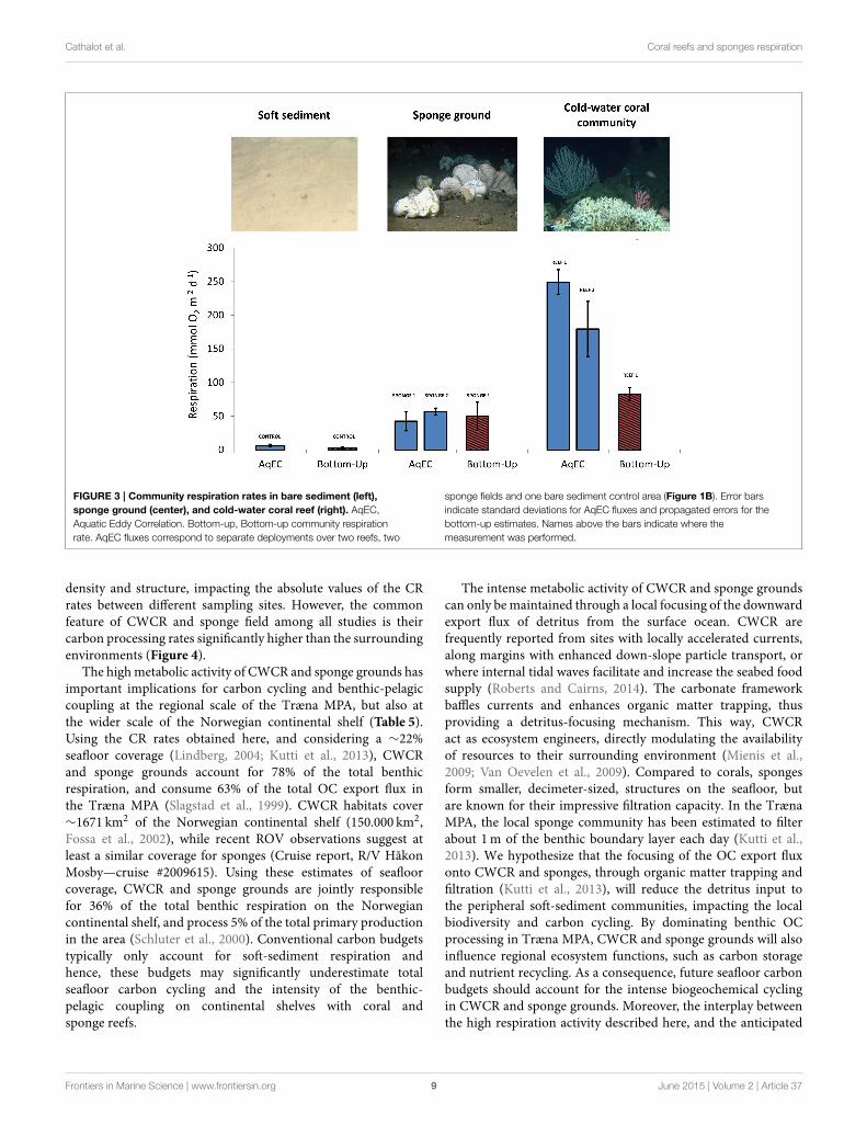
Community Respiration (CR) RatesRepresentative data time series obtained during AqECdeployments for the three habitat types (reef R1, spongeground S1 and control bare sediment C) are shown in Figure 2.Community Respiration (CR) rates, obtained by AqEC, differedby two orders of magnitude between the three habitats, revealingstrong differences in carbon processing rates (Figure 3). TheAqEC-based CR of the bare sediment site was 6 ± 2mmolO2 m−2 d−1 and compared favorably to CR obtained fromshipboard incubations of sediment cores (3 ± 1mmol O2

m−2 d−1). These low CR values are also consistent with rates(≈1mmolO2 m−2 d−1) previously reported for the Norwegiancontinental shelf at comparable water depths (Graf et al., 1995).AqEC-based CR rates within the sponge grounds were ∼10times higher (54 ± 5mmol O2 m−2 d−1) than the bare sedimentrates and compared well with the bottom-up estimate at thesponge ground site (48.7 ± 21.5mmol O2 m−2 d−1), whichwas obtained by combining and integrating the individualrespiration contributions of different habitat types within theAqEC footprint area (Table 3). CR rates over the coral reef weresystematically higher than in the adjacent bare sediments andsponge grounds (Figure 3). The highest AqEC-based CR rates(246 ± 18 and 177 ± 40mmol O2 m−2 d−1) were obtainedduring the deployments on the head part of the reef, which isdensely covered with living Lophelia pertusa (Figures 1B,D).The bottom-up CR estimates over CWCR (82 ± 10mmol O2

m−2 d−1; Table 4) are about 40% of these AqEC fluxes. However,comparing the two AqEC and bottom-up methods over the 5deployments (i.e., all 3 habitats), CR rates were not statisticallydifferent (p = 0.25, n = 5). Upscaling our AqEC measurementsto the whole reef structure (including the downstream tail partthat is less metabolically active) provided an average CR rateof 122 ± 10mmol O2 m−2 d−1 (Table 5), whereas upscaledbottom-up CR rates gave a value of 43 ± 7mmol O2 m−2 d−1.Ratios between the reef and the sediment CR rates were 20 and14, respectively for the AqEC and bottom-up technique. For thesponge habitat, ratios were of 9 and 16, respectively for the AqECand bottom-up estimates.

Discussion

Despite the complex topography of the reef structure and thesubstantial uncertainty associated with the “bottom-up” CRrates, the AqEC and bottom-up values align very well, andare not significantly different for the sponge ground and baresediment. However, AqEC technique did provide significantlyhigher CR rates than the “bottom-up” incubation methodover the reef habitats (Figure 3). This difference can be eitherdue to an overestimation on behalf of the AqEC technique,or equally, an underestimation associated with the bottomup incubation approach. Clearly, the bottom-up approachrequires a whole series of upscaling steps, where each upscalingstep introduces a new set of parameters (e.g., polyp density,local habitat cover), which each are associated with a givenuncertainty. These uncertainties eventually propagate throughthe upscaling process, which creates the possibility for asubstantial uncertainty on the final community respiration rate.On the other hand, the application of the AqEC techniqueover a topographically complex habitat, such as a cold-watercoral reef, is also challenging, and one should be vigilant thatthe basal assumptions underlying the AqEC technique are stillsatisfied. One critical assumption is that flow convergence orflow divergence are negligible, which is not necessarily thecase in an environment with complex and rough topography,such as coral reefs and sponge grounds. When present, flowconvergence/divergence may induce vertical velocity variationsthat can induce higher, spurious fluxes (Reimers et al., 2012;


http://www.rit.edu/cos/uphysics/uncertainties/Uncertaintiespart2.html

http://www.rit.edu/cos/uphysics/uncertainties/Uncertaintiespart2.html





TABLE 4 | Structure and Community Respiration (CR) rates of Reef R1 based on ROV video survey images and incubation rates.

Compartment Respiration rate

(mmolO2 m−2 d−1)

Living coral A 77.0 ± 12.8

Dead coral B 13.7 ± 1.6

Coral rubble C 3.3 ± 1.0

Habitat type Aeral contribution Formula Habitat CR rates Aeral coral CR rates

(%) (mmolO2 m−2 d−1) (mmolO2 m−2 d−1)

Live coral 53 A+ B+ C 139.2 ± 18.3 73.8 ± 9.7

Mixed live and dead coral framework 8 (A+B)2 + B+ C 62.2 ± 13.1 5.0 ± 1.0

Dead coral framework 12 B+ C 16.9 ± 1.9 2.0 ± 0.2

Coral rubble 27 C 3.3 ± 1.0 0.9 ± 0.3

Total 81.7 ± 9.8

Each habitat CR rates is calculated as the sum of its different compartments (Formula). Areal habitat CR rates are each individual habitat CR rates scaled-up to the entire reef using their

respective surface area contribution.

Lorke et al., 2013). We specifically assessed the importance offlow divergence at the reef site, by implementing a planar fitrotation to the ADV velocity data. This coordinate rotation alignsthe mean horizontal velocity along the main streamline andhence one does not need to invoke any assumption regardingthe flow field (Lorke et al., 2013). We found that the AqECfluxes did not change after the application of the planar fitrotation, which hence suggests a negligible impact of flowdivergence on the fluxes. Moreover, hydraulic studies examiningthe influence of forward facing steps on the flow pattern (Renand Wu, 2011), have shown that for similar Reynolds numbers(Re ∼400) as over the reefs, the effect of flow divergencebecomes negligible after ∼1.5 times the length of the step (inour case about 7 ∗ 1.5 = 10.5m, while the AqEC lander herewas positioned 20 meters behind the 7 meter step increase).Accordingly, we believe that flux divergence was most likelynegligible in our reef measurement, but future studies couldhowever consider a more detailed and more extensive evaluationof the AqEC technique in topographically complex environmentslike coral reefs (e.g., by placing multiple instruments inparallel, or examining whether the flux at different sensorheights).

Both the bottom-up approach and the AqEC methods showthat the CR rates on the reef and sponge grounds are substantiallyelevated compared to the bare sediment control site. Thesehigh CR rates evidently suggest intensified organic processingwithin the CWCR and sponge grounds of the Traena MPA.Based on our AqEC rates (which we consider more reliable thanthe corresponding bottom up estimates), community respirationin CWCR and sponge grounds are, respectively, ∼20 and ∼9times higher than those of the surrounding soft sediments.The observation that CWCR and sponge grounds function ashotspots of respiration is supported by indirect estimates ofcommunity respiration at other locations in the North Atlantic(Van Oevelen et al., 2009; White et al., 2012). Recently, Rovelliet al. (2015) reported respiration rates up to 46mmol O2m−2

d−1 in CWCR habitats in the Stjernsund area on the Norwegianshelf, which were also significantly higher than within adjacentbare sediment areas. If we compare the few available data againsta global compilation of soft sediment data, CWCR and spongegrounds clearly stand out by their high community respirationrates (Figure 4), although it is clear that there is variability amongthe few CR rates available in the literature. Indeed, CWCR andsponge ground sites can differ significantly both in terms in






FIGURE 3 | Community respiration rates in bare sediment (left),

sponge ground (center), and cold-water coral reef (right). AqEC,

Aquatic Eddy Correlation. Bottom-up, Bottom-up community respiration

rate. AqEC fluxes correspond to separate deployments over two reefs, two

sponge fields and one bare sediment control area (Figure 1B). Error bars

indicate standard deviations for AqEC fluxes and propagated errors for the

bottom-up estimates. Names above the bars indicate where the

measurement was performed.

density and structure, impacting the absolute values of the CRrates between different sampling sites. However, the commonfeature of CWCR and sponge field among all studies is theircarbon processing rates significantly higher than the surroundingenvironments (Figure 4).

The highmetabolic activity of CWCR and sponge grounds hasimportant implications for carbon cycling and benthic-pelagiccoupling at the regional scale of the Træna MPA, but also atthe wider scale of the Norwegian continental shelf (Table 5).Using the CR rates obtained here, and considering a ∼22%seafloor coverage (Lindberg, 2004; Kutti et al., 2013), CWCRand sponge grounds account for 78% of the total benthicrespiration, and consume 63% of the total OC export flux inthe Træna MPA (Slagstad et al., 1999). CWCR habitats cover∼1671 km2 of the Norwegian continental shelf (150.000 km2,Fossa et al., 2002), while recent ROV observations suggest atleast a similar coverage for sponges (Cruise report, R/V HåkonMosby—cruise #2009615). Using these estimates of seafloorcoverage, CWCR and sponge grounds are jointly responsiblefor 36% of the total benthic respiration on the Norwegiancontinental shelf, and process 5% of the total primary productionin the area (Schluter et al., 2000). Conventional carbon budgetstypically only account for soft-sediment respiration andhence, these budgets may significantly underestimate totalseafloor carbon cycling and the intensity of the benthic-pelagic coupling on continental shelves with coral andsponge reefs.

The intense metabolic activity of CWCR and sponge groundscan only bemaintained through a local focusing of the downwardexport flux of detritus from the surface ocean. CWCR arefrequently reported from sites with locally accelerated currents,along margins with enhanced down-slope particle transport, orwhere internal tidal waves facilitate and increase the seabed foodsupply (Roberts and Cairns, 2014). The carbonate frameworkbaffles currents and enhances organic matter trapping, thusproviding a detritus-focusing mechanism. This way, CWCRact as ecosystem engineers, directly modulating the availabilityof resources to their surrounding environment (Mienis et al.,2009; Van Oevelen et al., 2009). Compared to corals, spongesform smaller, decimeter-sized, structures on the seafloor, butare known for their impressive filtration capacity. In the TrænaMPA, the local sponge community has been estimated to filterabout 1m of the benthic boundary layer each day (Kutti et al.,2013). We hypothesize that the focusing of the OC export fluxonto CWCR and sponges, through organic matter trapping andfiltration (Kutti et al., 2013), will reduce the detritus input tothe peripheral soft-sediment communities, impacting the localbiodiversity and carbon cycling. By dominating benthic OCprocessing in Træna MPA, CWCR and sponge grounds will alsoinfluence regional ecosystem functions, such as carbon storageand nutrient recycling. As a consequence, future seafloor carbonbudgets should account for the intense biogeochemical cyclingin CWCR and sponge grounds. Moreover, the interplay betweenthe high respiration activity described here, and the anticipated






TABLE 5 | Carbon budget over the Traena Marine Protected Area (MPA), and the Norwegian Continental Shelf.

Benthic oxygen uptake rate* Benthic carbon uptake rate+ Area C demand % Resp % Export OC†

mmolO2m−2d−1 gC m−2 y−1 km2 103 tC y−1 % %

avg std avg std avg std

Traena MPA

Bare sediment 3.6 ± 0.9 12.0 ± 3.0 251 3.0 ± 0.8 21.5 17.3

CWCR 121.5 ± 9.9 408.6 ± 33.2 4 1.5 ± 0.1 10.7 8.6

Sponges 54.4 ± 4.7 183.1 ± 15.8 52 9.5 ± 0.8 67.7 54.4

Total 307 14

Norwegian continental shelf % Resp % PP‡

Bare sediment 146658 1764 ± 439 63.5 10.3

CWCR 1671a 683 ± 55 25.2 4.1

Sponges 1671b 306 ± 26 11.3 1.8

Total 150000c 2753

Comparison between the AqEC respiration rates and the Organic Carbon (OC) export flux and Primary Production (PP). *Benthic respiration rates based on our AqEC measurements.

Benthic oxygen uptake for bare sediment was however calculated as the average of our AqEC fluxes and bottom-up rates taking into account the variance of each (see the error

propagation section). +Respiratory quotient: 0.77 (Froelich et al., 1979).†Total export flux: 57 gCm−2 y−1 (Slagstad et al., 1999).

‡Primary Production: 112.7 gC m−2 y−1 (Schluter

et al., 2000).aFrom (Fossa et al., 2002).bBased on (Klitgaard and Tendal, 2004), we assumed a similar coverage for sponges than for corals.cFrom (Schluter et al., 2000; Huthnance, 2010).

FIGURE 4 | Community Respiration Rates in cold-water coral reefs

plotted against a compilation of soft sediment data (�) as a function of

water depth. Tisler Reef (△) (Wagner et al., 2011)—Rockall Bank (¿ ) (Van

Oevelen et al., 2009)—Mingulay Reef (©) (Maier et al., 2009)—Hatton Bank

(� , Van Oevelen, unpublished data)—Træna Reef ¢ , this study)—Mingulay

Reef (¿ ) (Rovelli et al., 2015)—Stjernsund (¯) (Rovelli et al., 2015). Sponge

ground data for Tranea reef are also included (Ø ). The solid line shows an

empirical model fit (double-exponential decrease with water depth) to the

compiled soft sediment data (Andersson et al., 2004).

climate feedbacks on organic matter export from the surfaceocean flux (Bopp et al., 2001), emphasize the sensitivity of deep-sea communities to climate change (Roberts and Cairns, 2014).

Author Contributions

GD, DV, and FM designed the study. CC performed AqECmeasurements. CC and TC analyzed the AqEC output data.ML and DV performed ship-board respiration incubations. TKperformed sponge respiration rates measurements and analysisof ROV images. CC, DV, and FM wrote the manuscript. Allauthors contributed substantially to the discussion of the resultsand revision of the manuscript.

Acknowledgments

We thank the crew and technical assistants of the RV HåkonMosby for their support at sea and during the operation ofthe ROV Aglanta. This research was funded by CoralFISH,a project in the European Community’s Seventh FrameworkProgramme (FP7/ 2007-2013) under grant agreement number213144, Odysseus grant G.0929.08 (FWO, Belgium) to FJRM,VIDI grant 864.08.004 (NWO, The Netherlands) to FJRM andVIDI grant 864.13.007 (NWO, The Netherlands) to DV.

Supplementary Material

The Supplementary Material for this article can be foundonline at: http://journal.frontiersin.org/article/10.3389/fmars.2015.00037/abstract

















References

Althaus, F., Williams, A., Schlacher, T. A., Kloser, R. J., Green, M. A., Barker,B. A., et al. (2009). Impacts of bottom trawling on deep-coral ecosystemsof seamounts are long-lasting. Mar. Ecol. Prog. Ser. 397, 279–294. doi:10.3354/meps08248

Andersson, J. H., Wijsman, J. W. M., Herman, P. M. J., Middelburg, J. J., Soetaert,K., and Heip, C. (2004). Respiration patterns in the deep ocean. Geophys. Res.Lett. 31, L03304. doi: 10.1029/2003GL018756

Attard, K. M., Glud, R. N., Mcginnis, D., and Rysgaard, S. (2014). Seasonal ratesof benthic primary production in a Greenland fjord measured by aquatic eddycorrelation. Limnol. Oceanogr. 59, 1555–1569. doi: 10.4319/lo.2014.59.5.1555

Berg, P., Glud, R. N., Hume, A., Ståhl, H., Oguri, K., Meyer, V., et al. (2009). Eddycorrelation measurements of oxygen uptake in deep ocean sediments. Limnol.

Oceanogr. Methods 7, 576–584. doi: 10.4319/lom.2009.7.576Berg, P., Røy, H., Janssen, F., Meyer, V., Jørgensen, B. B., Huettel, M., et al.

(2003). Oxygen uptake by aquatic sediments measured with a novel non-invasive eddy-correlation technique. Mar. Ecol. Prog. Ser. 261, 75–83. doi:10.3354/meps261075

Berg, P., Roy, H., and Wiberg, P. L. (2007). Eddy correlation flux measurements:the sediment surface area that contributes to the flux. Limnol. Oceanogr. 52,1672–1684. doi: 10.4319/lo.2007.52.4.1672

Bopp, L., Monfray, P., Aumont, O., Dufresne, J. L., Le Treut, H., Madec, G., et al.(2001). Potential impact of climate change onmarine export production.GlobalBiogeochem. Cycles 15, 81–99. doi: 10.1029/1999GB001256

Buhl-Mortensen, L., Vanreusel, A., Gooday, A. J., Levin, L. A., Priede, I. G.,Buhl-Mortensen, P., et al. (2010). Biological structures as a source of habitatheterogeneity and biodiversity on the deep ocean margins. Mar. Ecol. Evolut.

Perspect. 31, 21–50. doi: 10.1111/j.1439-0485.2010.00359.xDodds, L. A., Roberts, J. M., Taylor, A. C., and Marubini, F. (2007). Metabolic

tolerance of the cold-water coral Lophelia pertusa (Scleractinia) to temperatureand dissolved oxygen change. J. Exp. Mar. Biol. Ecol. 349, 205–214. doi:10.1016/j.jembe.2007.05.013

Fisher, C. R., Hsing, P.-Y., Kaiser, C. L., Yoerger, D. R., Roberts, H. H., Shedd,W. W., et al. (2014). Footprint of Deepwater Horizon blowout impact to deep-water coral communities. Proc. Natl. Acad. Sci. U.S.A. 111, 11744–11749. doi:10.1073/pnas.1403492111

Fossa, J. H., Mortensen, P. B., and Furevik, D. M. (2002). The deep-watercoral Lophelia pertusa in Norwegian waters: distribution and fishery impacts.Hydrobiologia 471, 1–12. doi: 10.1023/A:1016504430684

Froelich, P. N., Klinkhammer, G. P., Bender, M. L., Luedtke, N. A., Heath, G. R.;,Cullen, D., et al. (1979). Early oxidation of organic matter in pelagic sedimentsof the eastern equatorial Atlantic: suboxic diagenesis. Geochim. Cosmochim.

Acta 43, 1075–1090. doi: 10.1016/0016-7037(79)90095-4Graf, G., Gerlach, S. A., Ritzrau, W., Scheltz, A., Linke, P., Thomsen, L.,

et al. (1995). Benthic-pelagic coupling in the Greenland Norwegian Sea andits effect on the geological record. Geologische Rundschau 84, 49–58. doi:10.1007/BF00192241

Grasshoff, K. (ed.). (1976). Methods of Seawater Analysis. Weinheim; New York:Verlag Chemie.

Hume, A., Berg, P., and McGlathery, K. J. (2011). Dissolved oxygen fluxes andecosystem metabolism in an eelgrass (Zostera marina) meadow measuredwith the eddy correlation technique. Limnol. Oceanogr. 56, 86–96. doi:10.4319/lo.2011.56.1.0086

Huthnance, J. M. (2010). “5.2. The Northeast Atlantic margins,” in Carbon and

Nutrient Fluxes in Continental Margins: A Global Synthesis, eds K. K. Liu,L. Atkinson, R. Quinones, and L. Talaue-Mcmanus (Berlin: Springer-Verlag),215–234.

Kim, S. C., Friedrichs, C. T., Maa, J. P.-Y., and andWright, L. D. (2000). Estimatingbottom stress in tidal boundary layer from acoustic doppler velocimeter data.J. Hydraul. Eng. 126, 399–406. doi: 10.1061/(ASCE)0733-9429(2000)126:6(399)

Klitgaard, A. B., and Tendal, O. S. (2004). Distribution and species compositionof mass occurrences of large-sized sponges in the northeast Atlantic. Prog.Oceanogr. 61, 57–98. doi: 10.1016/j.pocean.2004.06.002

Kutti, T., Bannister, R. J., and Fossa, J. H. (2013). Community structure andecological function of deep-water sponge grounds in the Traenadypet MPA-Northern Norwegian continental shelf. Cont. Shelf Res. 69, 21–30. doi:10.1016/j.csr.2013.09.011

Kutti, T., Bergstad, O. A., Fossa, J. H., and Helle, K. (2014). Cold-watercoral mounds and sponge-beds as habitats for demersal fish on theNorwegian shelf. Deep Sea Res. II Top. Stud. Oceanogr. 99, 122–133. doi:10.1016/j.dsr2.2013.07.021

Laberg, J. S., Vorren, T. O., Mienert, J., Bryn, P., and Lien, R. (2002). TheTraenadjupet Slide: a large slope failure affecting the continental margin ofNorway 4,000 years ago. Geo-Mar. Lett. 22, 19–24. doi: 10.1007/s00367-002-0092-z

Lindberg, B. (2004). Cold-Water Coral Reefs on the Norwegian Shelf - Acoustic

Signature, Geological, Geomorphological and Environmental Setting. Ph.D.,University of Tromsø.

Long, M. H., Berg, P., De Beer, D., and Zieman, J. C. (2013). In situ coralreef oxygen metabolism: an eddy correlation study. PLoS ONE 8:e58581. doi:10.1371/journal.pone.0058581

Lorke, A., McGinnis, D. F., and Maeck, A. (2013). Eddy-correlation measurementsof benthic fluxes under complex flow conditions: effects of coordinatetransformations and averaging time scales. Limnol. Oceanogr. Methods 11,425–437. doi: 10.4319/lom.2013.11.425

Lorrai, C., Mcginnis, D. F., Berg, P., Brand, A., and Wuest, A. (2010). Applicationof oxygen eddy correlation in aquatic systems. J. Atmos. Ocean. Technol. 27,1533–1546. doi: 10.1175/2010JTECHO723.1

Maier, C., Hegeman, J., Weinbauer, M. G., and Gattuso, J. P. (2009). Calcificationof the cold-water coral Lophelia pertusa under ambient and reduced pH.Biogeosciences 6, 1671–1680. doi: 10.5194/bg-6-1671-2009

Mcginnis, D. F., Berg, P., Brand, A., Lorrai, C., Edmonds, T. J., and Wuest, A.(2008). Measurements of eddy correlation oxygen fluxes in shallow freshwaters:towards routine applications and analysis. Geophys. Res. Lett. 35, L04403. doi:10.1029/2007GL032747

Mienis, F., De Stigter, H. C., De Haas, H., and Van Weering, T. C. E. (2009). Near-bed particle deposition and resuspension in a cold-water coral mound area atthe Southwest Rockall Trough margin, NE Atlantic. Deep Sea Res. I Oceanogr.

Res. Pap. 56, 1026–1038. doi: 10.1016/j.dsr.2009.01.006Miller, R. J., Hocevar, J., Stone, R. P., and Fedorov, D. V. (2012). Structure-

forming corals and sponges and their use as fish habitat in bering sea submarinecanyons. PLoS ONE 7:e33885. doi: 10.1371/journal.pone.0033885

Purser, A., and Thomsen, L. (2012). Monitoring strategies for drill cuttingdischarge in the vicinity of cold-water coral ecosystems. Mar. Pollut. Bull. 64,2309–2316. doi: 10.1016/j.marpolbul.2012.08.003

Pusceddu, A., Bianchelli, S., Martin, J., Puig, P., Palanques, A., Masque, P., et al.(2014). Chronic and intensive bottom trawling impairs deep-sea biodiversityand ecosystem functioning. Proc. Natl. Acad. Sci. U.S.A. 111, 8861–8866. doi:10.1073/pnas.1405454111

Reba, M. L., Link, T. E., Marks, D., and Pomeroy, J. (2009). An assessmentof corrections for eddy covariance measured turbulent fluxes oversnow in mountain environments. Water Resour. Res. 45, W00D38. doi:10.1029/2008WR007045

Reimers, C. E., H. T. Özkan-Haller, P., Berg, A., Devol, K., andMcCann-Grosvenor,and, R. D., Sanders (2012). Benthic oxygen consumption rates during hypoxicconditions on the Oregon continental shelf: evaluation of the eddy correlationmethod. J. Geophys. Res. 117, C02021. doi: 10.1029/2011jc007564

Ren, H., and Wu, Y. (2011). Turbulent boundary layers over smooth and roughforward-facing steps. Phys. Fluids 23, 045102. doi: 10.1063/1.3576911

Roberts, J. M., and Cairns, S. D. (2014). Cold-water corals in a changing ocean.Curr. Opin. Environ. Sustain. 7, 118–126. doi: 10.1016/j.cosust.2014.01.004

Roberts, J. M., Wheeler, A. J., and Freiwald, A. (2006). Reefs of the deep: thebiology and geology of cold-water coral ecosystems. Science 312, 543–547. doi:10.1126/science.1119861

Rovelli, L., Attard, K., Bryant, L. D., Flögel, S., Stahl, H., Roberts, J. M., et al. (2015).Benthic O2 uptake of two cold-water coral communities estimated with thenon-invasive eddy correlation technique.Mar. Ecol. Prog. Ser. 525, 97–104. doi:10.3354/meps11211

Schluter, M., Sauter, E. J., Schafer, A., and Ritzrau, W. (2000). Spatial budgetof organic carbon flux to the seafloor of the northern North Atlantic(60 degrees N-80 degrees N). Global Biogeochem. Cycles 14, 329–340. doi:10.1029/1999GB900043

Slagstad, D., Tande, K. S., and Wassmann, P. (1999). Modelled carbon fluxes asvalidated by field data on the north Norwegian shelf during the productiveperiod in 1994. Sarsia 84, 303–317.






Tjensvoll, I., Kutti, T., Fosså, J. H., and Bannister, R. J. (2013). Rapid respiratoryresponses of the deep-water sponge Geodia barretti exposed to suspendedsediments. Aquat. Biol. 19, 65–73. doi: 10.3354/ab00522

Van Oevelen, D., Duineveld, G., Lavaleye, M., Mienis, F., Soetaert, K., andHeip, C. H. R. (2009). The cold-water coral community as a hot spot forcarbon cycling on continental margins: a food-web analysis from Rockall Bank(northeast Atlantic). Limnol. Oceanogr. 54, 1829–1844. doi: 10.4319/lo.2009.54.6.1829

Wagner, H., Purser, A., Thomsen, L., Jesus, C. C., and Lundalv, T. (2011).Particulate organic matter fluxes and hydrodynamics at the Tisler cold-water coral reef. J. Mar. Syst. 85, 19–29. doi: 10.1016/j.jmarsys.2010.11.003

White, M., Wolff, G. A., Lundalv, T., Guihen, D., Kiriakoulakis, K., Lavaleye, M.S. S., et al. (2012). Cold-water coral ecosystem (Tisler Reef, Norwegian Shelf)

may be a hotspot for carbon cycling. Mar. Ecol. Prog. Ser. 465, 11–23. doi:10.3354/meps09888

Conflict of Interest Statement: The authors declare that the research wasconducted in the absence of any commercial or financial relationships that couldbe construed as a potential conflict of interest.

Copyright © 2015 Cathalot, Van Oevelen, Cox, Kutti, Lavaleye, Duineveld and

Meysman. This is an open-access article distributed under the terms of the Creative

Commons Attribution License (CC BY). The use, distribution or reproduction in

other forums is permitted, provided the original author(s) or licensor are credited

and that the original publication in this journal is cited, in accordance with accepted

academic practice. No use, distribution or reproduction is permitted which does not

comply with these terms.


http://creativecommons.org/licenses/by/4.0/








Documents

Cold-water coral reefs and adjacent sponge grounds ... · PDF fileCold-water corals and sponges form complex reef structures on the seaﬂoor (Figure1), which support a rich community